Alma Mater Studiorum · Universita di Bologna

FACOLTA DI SCIENZE MATEMATICHE, FISICHE E NATURALI

Corso di Laurea Magistrale in Matematica

THE WIENER CRITERION

FOR THE LAPLACIANAND THE HEAT OPERATOR

Tesi di Laurea in

Analisi Matematica

Relatore:

Chiar.mo Prof.

Ermanno Lanconelli

Presentata da:

Paola Elefante

II Sessione

Anno Accademico 2010-2011

Sommario

La tesi presenta il criterio di regolarita di Wiener nell’ambito classico

dell’operatore di Laplace ed in seguito alcune nozioni di teoria del

potenziale e la dimostrazione del criterio nel caso dell’operatore del calore;

in questa seconda sezione viene dedicata particolare attenzione alle formule

di media e ad una diseguaglianza forte di Harnack, che risultano

fondamentali nella trattazione dell’argomento centrale.

A mamma Daniela

e babbo Pino.

Introduction

The classical Dirichlet problem offers two sides, the first is the deter-

mination of the harmonic function corresponding to given boundary values,

while the second is the analysis of the behaviour of this map near the bound-

ary. Both Norbert Wiener and Henri Lebesgue pointed out this aspect of

the problem in 1924 and in the same year the first one came up with a brand

new characterization of regular points ([21]), i.e. a point x0 ∈ ∂Ω (Ω ⊂ Rn

open set) is regular if and only if the series

∞∑

k=1

λk cap(Ωc ∩ λk ≤ |x− x0|2−n ≤ λk+1)

diverges for some λ > 1, where cap(·) is the Choquet capacity. The first

chapter of this thesis shows the basic definitions and the main concepts of

potential theory for the Laplace operator ∆, some properties of the Cho-

quet capacity, then goes through some other characterizations of regular

points and ends with the already mentioned Wiener’s criterion. In the sec-

ond chapter some more recent results are presented: the heat operator (and,

in general operators of parabolic type) shows some basic features that are

deeply different from the laplacian and needs a different approach. A whole

potential theory was developed and the corresponding Wiener’s criterion

was stated. The works Bruno Pini were fundamental in the development of

this field: in his work [14] of 1951,for instance, he proved a mean formula

for the solutions of some parabolic operators by using the level surfaces of

the fundamental solution. These formulas were used to characterize tem-

peratures in a new way (see [16]). The formula proved by Pini was later

extended to the case of several spatial dimensions later by Montaldo (1955),

Fulks (1961) and Watson (1971); in this thesis we will show that it has a

i

fundamental role in the proof of the criterion. Another pillar of the heat

operator theory is the Harnack inequality, proved indipendently by Pini and

Hadarmard in 1954.

The criterion for the heat equation takes the following form: a point z0 ∈∂Ω ⊂ R

n+1, (Ω bounded open set) is regular if and only if the series

∞∑

k=1

λk capH(Ωc ∩ λk+1 ≥ K(z0 − z) ≥ λk) = +∞ for some λ > 1

where K is the fundamental solution with pole at (0, 0) and capH is the

thermal capacity, analogous to the Choquet capacity of the theory of har-

monic functions.

In his investigations, Pini was able to give several sufficient conditions of

regularity and irregularity for some open subsets of Rn+1, but it was in 1973

that Ermanno Lanconelli ([11]) proved the necessity of the criterion for any

bounded open set Ω ⊂ Rn+1; the proof of the criterion was completed later

in 1980 by Lawrence C. Evans and Ronald F. Gariepy ([4]), who used some

mean formulas and a kind of strong Harnack inequality.

ii

Contents

1 Wiener’s criterion for the Laplace operator 1

1.1 The Perron-Wiener-Brelot method . . . . . . . . . . . . . . . 1

1.2 Preliminaries . . . . . . . . . . . . . . . . . . . . . . . . . . . 2

1.3 Characterization of regular points . . . . . . . . . . . . . . . . 5

2 Wiener’s criterion for the heat equation 13

2.1 Preliminaries . . . . . . . . . . . . . . . . . . . . . . . . . . . 13

2.2 Properties of thermal capacity and potentials . . . . . . . . . 15

2.3 Properties of the sets Ω(c) . . . . . . . . . . . . . . . . . . . . 19

2.4 Mean-value formulas and strong Harnack inequality . . . . . 20

2.5 Necessity of (2.4) . . . . . . . . . . . . . . . . . . . . . . . . . 29

2.6 Sufficiency of (2.4) . . . . . . . . . . . . . . . . . . . . . . . . 31

Bibliography 43

iii

iv

Chapter 1

Wiener’s criterion for the

Laplace operator

1.1 The Perron-Wiener-Brelot method

Let Ω ⊂ Rn(n > 2) be an open set and f a continuous function on ∂Ω;

we denote by U(Ω) the set of all superharmonic functions on Ω and by L(Ω)

the set of subharmonic functions on Ω1. Call the objects

Hf = infv ∈ U(Ω), lim infΩ∋y→x

v(y) ≥ f(x) for any x ∈ ∂Ω

Hf = supv ∈ L(Ω), lim supΩ∋y→x

v(y) ≤ f(x) for any x ∈ ∂Ω

respectively the upper solution and the lower solution to the generalized

Dirichlet problem with boundary value f :

∆u = 0 on Ω

u = f on ∂Ω(1.1)

It happens that Hf ≤ Hf if Ω is a bounded open set (see [9], lemma (8.2)).

A function f ∈ C(∂Ω) is called resolutive if Hf = Hf =: Hf and they are

finite-valued. One can prove Hf is harmonic (see for example [1], chapter

6); Hf is called the Perron-Wiener-Brelot solution to the Dirichlet problem

(1.1).

1We ask superharmonic functions not to be identically +∞ on any component of Ω.

1

Wiener proved that every continuous function defined on the boundary of a

bounded open set is resolutive (see [9], theorem (8.11) for a proof).

1.2 Preliminaries

In all our discussion we will be working in Rn with n > 2. Let F ⊂ R

n

be a compact subset of Ω. Pick u ∈ U(Ω), u ≥ 0 and put:

ΦuF := v ∈ U(Rn) : v ≥ 0 on R

n, v ≥ u on F

RuF (x) := inf

v∈ΦuF

v(x)

RuF is called the reduced function (or reduite) of u relative to F in R

n.

In general, RuF is not lower semicontinuous (l.s.c.): consider the fundamental

solution Uy(x) = |x − y|2−n with pole at y, take Ω = Rn, F = y. Then

one has

RUy

F (x) =

0 x 6= y

+∞ x = y

and hence it is not l.s.c..

This is why we define the regularized reduced function (or balayage) of u

relative to F on Rn as:

RuF (x) = lim inf

y→xRu

F (y) x ∈ Rn

From now on we will denote by WF = R1F , VF = R1

F where F is a compact

set as above. Let us state some basic properties of these new objects.

Lemma 1.2.1. With the same notations as before:

(i) 0 ≤ VF ≤ WF ≤ 1.

(ii) WF = 1 on F .

(iii) VF = WF on intF ∪ F c.

(iv) One has

limΩ∋|y|→∞

VF (y) = limΩ∋|y|→∞

WF (y) = 0

except for a polar set (see the definiton later).

2

(v) VF is superharmonic on Ω and harmonic on F c.

Proof. Since 1 ∈ Φ1F , by definition of VF and WF one sees immediately that

VF ≤ WF ≤ 1. Plus, as the elements of Φ1F are non-negative, one must have

VF ≥ 0. By definition, it is obvious that WF = 1 on F , as v ≥ 1 on F for

any v ∈ Φ1F ; as WF is constantly 1 on intF , VF must be identically 1 there

as well.

Helms proves the rest of this theorem in [9], chapter 7.

Denote by M+(F ) the set of all non-negative Radon measures with sup-

port contained in F . For any µ ∈ M+(F ) we define the µ-Green potential :

Gµ(x) =

ˆ

Rn

|x− y|2−ndµ(y)

Now set:

cap(F ) = supµ(Rn) : µ ∈ M+(F ), Gµ ≤ 1 on R

n

Theorem 1.2.2. For any compact sets F,F ′ ⊂ Rn, one has:

(i) cap(F ) < ∞.

(ii) cap(F ∪ F ′) ≤ cap(F ) + cap(F ′).

(iii) If F ⊂ F ′ then cap(F ) ≤ cap(F ′).

(iv) If Fll∈N is a decreasing sequence of compact sets and F =

∞⋂

l=1

Fl, one

has liml→∞

cap(Fl) = cap(F ).

Proof. (i): as F is compact, we can pick x0 ∈ F c. Then x 7→ G(x0, x) ≥ 0

is harmonic on a neighbourhood of F and hence by maximum principle

G(x0, x) > ǫ > 0 on F for some ǫ. Set α := infx∈F

G(x0, x) > 0; for any

µ ∈ M+(F ) such that Gµ ≤ 1 one has:

αµ(F ) = infx∈F

G(x0, x)

ˆ

Rn

dµ(y) ≤ˆ

Rn

G(x0, y)dµ(y) = Gµ(x0) ≤ 1 ⇒ µ(F ) ≤ 1

α

and this proves the finiteness of cap(F ).

(ii): pick one µ ∈ M+(F ∪ F ′) such that µ(Rn) = cap(F ∪ F ′). Obviously

µ|F ∈ M+(F ), Gµ|F

≤ Gµ ≤ 1 and the same happens for µ|F ′ ; hence we have

cap(F ∪ F ′) = µ(F ∪ F ′) ≤ µ(F ) + µ(F ′) ≤ cap(F ) + cap(F ′)

3

(iii): this holds because

µ ∈ M

+(F ), Gµ ≤ 1 on Rn⊂

µ ∈ M

+(F ′), Gµ ≤ 1 on Rn

(iv): see (??), theorem (5.4.2) for a proof.

We now state a very important result.

Theorem 1.2.3. Let F ⊂ Rn be compact. There exists a unique µ⋆ ∈

M+(F ) such that:

(i) Gµ⋆ = VF .

(ii) cap(F ) = µ⋆(Rn).

(iii) Gµ ≤ Gµ⋆ for any µ ∈ M+(F ) such that Gµ ≤ 1.

We call µ⋆ the capacitary distribution of F and VF the capacitary poten-

tial for F .

It is possibile to define a capacity for any subset E of Rn; we call inner

capacity of E the quantity:

cap⋆(E) = supcap(F ) : F ⊂ E,F compact

Similarly, the outer capacity of E is defined as

cap⋆(E) = infcap⋆(U) : E ⊂ U,U open

A set E ⊂ Rn is said to be capacitable if cap⋆(E) = cap⋆(E) and we call

capacity of E the quantity cap(E) := cap⋆(E).

Lemma 1.2.4. All open and compact subsets of Rn are capacitable.

Proof. If U ⊂ Rn is open, cap⋆(U) = cap⋆(U) by definition. Let F ⊂ R

n

be compact; obviously cap⋆(F ) = cap(F ) accordingly to the definition of

capacity of compact sets given at first. For any ǫ > 0, there exist U so that

if F ′ is compact and F ⊂ F ′ ⊂ U , one has cap(F ′) ≤ cap(F ) + ǫ. Hence:

cap(F ′) = cap⋆(F′) ≤ cap⋆(U) = sup

F ′′⊂Ucap(F ′′) ≤ cap(F ) + ǫ

4

For any open set V such that F ⊂ V ⊂ U one gets cap⋆(F ) ≤ cap⋆(V ) ≤cap⋆(U) and therefore

cap(F ) = cap⋆(F ) ≤ infV⊃F

cap⋆(V ) = cap⋆(F ) ≤ cap⋆(U) ≤ cap(F ) + ǫ

This is true for any ǫ > 0, so cap(F ) = cap⋆(F ).

If ω ⊂ Rn is such that cap⋆(ω) = 0 we call it a polar set.

Lemma 1.2.5. If ω ⊂ Rn and u ≥ 0 is a superharmonic function on R

n it

occurs that

Ruω = Ru

ω

except for a polar set Z ⊂ ∂ω.

Proof. See [9], corollary (7.40).

1.3 Characterization of regular points

Let Ω ⊂ Rn be an open set. A function w is a barrier at x0 ∈ ∂Ω if it

is defined on W ∩Ω for some neighbourhood W of x0 and has the following

properties:

1. w is superharmonic on W ∩ Ω.

2. w > 0 on W ∩ Ω.

3. limW∩Ω∋x→x0

w(x) = 0.

If x0 is a limit point of Ω, we say Ω is thin at x0 if there exist a su-

perharmonic function u on a neighbourhood of x0 such that 0 < u(x0) <

lim infΩ∋x→x0,x 6=x0

u(x) = +∞.

Lemma 1.3.1. Let Ω be thin at the limit point x0; then

VF (r)(x0) → 0 for r → 0+

where F (r) = Ω ∩B(x0, r).

5

Proof. By definition we know there exists a superharmonic function u such

that

0 < u(x0) < +∞ = lim infΩ∋x→x0,x 6=x0

u(x)

Choose ǫ > 0; we can pick r > 0 so that u(x) >u(x0)

ǫfor all x ∈ F (r)\x0.

The set x0 has capacity zero, hence VF (r) = VF (r)\x0 (see [1], theorem

(5.3.4)). By lemma (1.2.1)-(i) we know VF (r)(x) ≤ ǫu(x)

u(x0)on F (r) and

in particular VF (r′)(x0) ≤ VF (r)(x0) ≤ ǫ for any 0 < r′ < r, as F (r) is a

decreasing sequence.

Lemma 1.3.2. If Ω is not thin at x0 ∈ ∂Ω, then VF (r)(x0) = 1 for all r > 0.

Proof. If Ω is not thin at x0, by definition this means that for any super-

harmonic function v defined on a neighbourhood of x0, at least one of the

following statements holds:

(i) u(x0) = +∞.

(ii) u(x0) ≥ lim infΩ∋x→x0,x 6=x0

u(x).

(iii) lim infΩ∋x→x0,x 6=x0

u(x) < +∞

If we pick u = VF (r), we know the only possible case is 1 ≥ u(x0) ≥lim inf

Ω∋x→x0,x 6=x0

u(x) = 1, hence VF (r)(x0) = 1 for any r.

We say that the function u : D → [−∞,+∞] peaks at x0 ∈ D if

supu(x) : x ∈ D \B(x0, r) < u(x0)

for all r > 0 such that D \B(x0, r) 6= ∅.

Theorem 1.3.3. Let F ⊂ Ω and u ≥ 0, u ∈ U(Ω). Assume u peaks at

x0 ∈ Ω and u(x0) < ∞. Then F is thin at x0 if and only if RFu (y) < u(y).

Proof. See [1], theorem (7.3.4).

Theorem 1.3.4. Let Ω be a bounded open set that has a Green function

and x0 ∈ ∂Ω. Then the following statements are equivalent:

(i) x0 is a regular point.

6

(ii) There exists a barrier at x0.

(iii) Ωc is not thin at x0.

Proof. (i)⇔(ii): suppose at first x0 is regular and consider the map w(x) =

|x0 − x|, x ∈ ∂Ω; then by maximum principle the harmonic solution Hw is

such thatHw(x) ≥ |x−x0| ≥ 0 for any x ∈ Ω and if we prove limΩ∋x→x0

Hw(x) =

0, we can say it is a barrier at x0, but this is true as by assumption, we know

limΩ∋x→x0

Hw(x) = w(x0) = 0, because w is a continuous function on ∂Ω. Now

suppose there is a barrier at x0; for any bounded f on ∂Ω one has

lim supΩ∋x→x0

Hf (x) ≤ lim sup∂Ω∋x→x0

f(x)

lim infΩ∋x→x0

Hf (x) ≥ lim inf∂Ω∋x→x0

f(x)

(see [9], lemma (8.20) for a proof). If f is continuous, by applying this last

statement we get

lim infΩ∋x→x0

Hf (x) ≤ lim supΩ∋x→x0

Hf (x) ≤ f(x0) ≤ lim infΩ∋x→x0

Hf (x) ≤ lim infΩ∋x→x0

Hf (x)

hence limΩ∋x→x0

Hf (x) = f(x0); as lim infΩ∋x→x0

Hf (x) ≤ lim infΩ∋x→x0

Hf (x) one can

conclude that also limΩ∋x→x0

Hf (x) = f(x0), hence x0 is a regular point.

(i)⇔(iii): assume Ωc is not thin at x0 and consider the ball B = B(x0, 1).

Define the positive superharmonic function u(x) = 1−|x−x0|2 on B (∆u =

−2n < 0); now build the positive superharmonic function w := u− RuΩc∩B

where the balayage is with respect to B. w has to be strictly positive on

B ∩ Ω; in fact, if there is x ∈ B ∩ Ω such that w(x) = 0, by maximum

principle w = 0 on all B ∩Ω, hence u = RuΩc∩B there and by lemma (1.2.1)-

(v) u would be harmonic on B ∩Ω, but this would be a contradiction since

∆u < 0 there. As u peaks in x0, theorem (1.3.3) and the assumption imply

that w(x0) = 0, therefore w is a barrier at x0 and this implies x0 is regular.

Suppose now x0 is regular. Pick r′ small enough so that Ω′ := Ω∪B(x0, r′)

still has a Green function; for each 0 < r < r′ define

fr(x) =

1 x ∈ ∂Ω ∪B(x0, r)

0 x ∈ ∂Ω \B(x0, r)

7

Call E(r) the compact set B(x0, r) \Ω. Taking the reductions with respect

to Ω′ and recalling lemma (1.2.1):

1 = VE(r)(x) = WE(r)(x) ≥ Hfr(x) x ∈ int(E(r))

As x0 is regular, we have limΩ∋x→x0

Hfr(x) = fr(x0) = 1 hence VE(r)(x0) = 1

for all 0 < r < r′; by lemma (1.3.1) we know Ωc is not thin at x0.

We can now state a very important result that has an analogy in the the-

ory of the heat operator (see lemma (2.3.2), chapter 2) that is a fundamental

tool for various proofs.

Lemma 1.3.5. If Ω is a bounded open set with Green function, x0 ∈ ∂Ω is

regular if and only if

VF (r)(x0) = 1 ∀r > 0

Proof. It is enough to put together the results of lemma (1.3.1), lemma

(1.3.2) and theorem (1.3.4).

Theorem 1.3.6 (Wiener’s criterion). Let Ω ⊂ Rn be a bounded open set

and x0 ∈ ∂Ω. Then x0 is a regular boundary point of Ω if and only if

∞∑

k=1

λk cap(Ωc ∩ λk ≤ |x− x0|2−n ≤ λk+1) = +∞ for some λ > 1

Proof. Suppose at first that

∞∑

k=1

λk cap(Ck) < +∞

where we call Ωc ∩ λk ≤ |x− x0|2−n ≤ λk+1 =: Ck. As the regularity is a

local property, we can assume Ω ⊂ B := B(x0, 1). Let ǫll be a sequence

of positive numbers such that∞∑

k=1

λkǫk < ∞; for any k ∈ N call µk the

capacitary distribution of the compact set Ck and Vk = Gµkits capacitary

potential; recall that µk(Rn) = cap(Ck). Then

Vk(x0) =

ˆ

Ck

|y − x0|2−ndµk(y) ≤ λk+1 cap(Ck)

8

Figure 1.1: Proof of theorem (1.3.6).

As by assumption the series converges, we can choose k so that

Vk(x0) ≤ λ2∑

j≥k

cap(Cj) < 1

and by lemma (1.3.4) this makes us conclude that x0 is irregular.

Assume x0 is irregular; by thereom (1.3.4) this tells us there is a super-

harmonic function u such that 0 < u(x0) < +∞ = lim infΩ∋x→x0,x 6=x0

u(x); call

αk = infCk

u and fix arbitrarily a positive number α. Set

Vk = x : v(x) > αk − α ⊃ Ck

Uk = Vk ∩ λk ≤ |x− x0|2−n ≤ λk+1 ⊃ Ck

If we prove∞∑

k=1

λk cap⋆(Uk) < ∞ we are done, because Ck ⊂ Uk,∀k. Let

ǫll be a sequence of positive numbers such that∞∑

k=1

λkǫk < ∞ and for

any l ∈ N pick a compact set Kl ⊂ Ul such that cap⋆(Ul) < cap(Kl) + ǫl

(see figure 1.3.6). Then we need to prove∞∑

l=1

λl cap(Kl) < ∞. To do that,

9

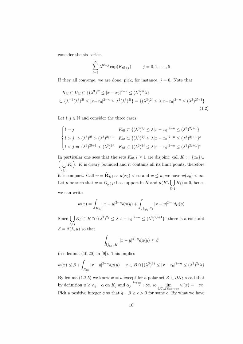
consider the six series:

∞∑

l=1

λ6l+j cap(K6l+j) j = 0, 1, · · · , 5

If they all converge, we are done; pick, for instance, j = 0. Note that

K6l ⊂ U6l ⊂ (λ3)2l ≤ |x− x0|2−n ≤ (λ3)2lλ⊂ λ−1(λ3)2l ≤ |x−x0|2−n ≤ λ2(λ3)2l = (λ3)2l ≤ λ|x−x0|2−n ≤ (λ3)2l+1

(1.2)

Let l, j ∈ N and consider the three cases:

l = j K6l ⊂ (λ3)2j ≤ λ|x− x0|2−n ≤ (λ3)2j+1

l > j ⇒ (λ3)2l > (λ3)2j+1 K6l ⊂ (λ3)2j ≤ λ|x− x0|2−n ≤ (λ3)2j+1c

l < j ⇒ (λ3)2l+1 < (λ3)2j K6l ⊂ (λ3)2j ≤ λ|x− x0|2−n ≤ (λ3)2j+1c

In particular one sees that the sets K6l, l ≥ 1 are disjoint; call K := x0 ∪(⋃

l≥1

Kl

). K is cleary bounded and it contains all its limit points, therefore

it is compact. Call w = RuK ; as u(x0) < ∞ and w ≤ u, we have w(x0) < ∞.

Let µ be such that w = Gµ; µ has support in K and µ(B \⋃

l≥1

Kl) = 0, hence

we can write

w(x) =

ˆ

K6j

|x− y|2−ndµ(y) +

ˆ

⋃l 6=j Kl

|x− y|2−ndµ(y)

Since⋃

l 6=j

Kl ⊂ B ∩ (λ3)2j ≤ λ|x − x0|2−n ≤ (λ3)2j+1c there is a constant

β = β(λ, µ) so thatˆ

⋃l 6=j Kl

|x− y|2−ndµ(y) ≤ β

(see lemma (10.20) in [9]). This implies

w(x) ≤ β+

ˆ

K6j

|x− y|2−ndµ(y) x ∈ B∩(λ3)2j ≤ |x−x0|2−n ≤ (λ3)2jλ

By lemma (1.2.5) we know w = u except for a polar set Z ⊂ ∂K; recall that

by definition u ≥ αj−α on Kj and αjj→∞−→ +∞, so lim

(K\Z)∋x→x0

w(x) = +∞.

Pick a positive integer q so that q− β ≥ ǫ > 0 for some ǫ. By what we have

10

proved above, there is j0 such that w(x) ≥ q for x ∈ K6j , j ≥ j0 except for

a polar set. Therefore

ˆ

K6j

|x− y|2−ndµ(y) ≥ ǫ x ∈ K6j , j ≥ j0

Claim: µ(K6j) ≥ ǫ cap(K6j) for all j ≥ j0. Call µ⋆ the capacitary distribu-

tion of K6j ; then

µ(K6j) =

ˆ

K6j

dµ ≥ˆ

K6j

Gµ⋆dµ =

ˆ

K6j

Gµdµ⋆ ≥ ǫ cap(K6j)

therefore ∑

j≥j0

λ6jµ(K6j) ≥ ǫ∑

j≥j0

λ6j cap(K6j) (1.3)

Notice that

∑

j≥j0

λ6jµ(K6j) ≤∑

j≥j0

ˆ

K6j

|x0 − x|2−ndµ(x) ≤ˆ

K|x0 − x|2−ndµ(x)

and

∞ > w(x0) =

ˆ

K|x− x0|2−ndµ(x)

therefore the original series converges.

11

12

Chapter 2

Wiener’s criterion for the

heat equation

2.1 Preliminaries

In this chapter we would like to show the proof of the Wiener’s test in

the case of the heat operator:

H = ∂t −∆x

in Rnx ×Rt. We denote by

K(x, t) =

1

(4πt)n/2e−

|x|2

4t t ≥ 0

0 t < 0

the fundamental solution of the heat operator with pole at (0, 0).

The next definitions and notions are parallel to the ones of the potential

theory of the Laplacian. Fix a bounded open set Ω ⊂ Rn+1.

A function u ∈ C2(Ω) is said to be a temperature in Ω if Hu = 0 on Ω.

A bounded open set U ⊂ Rn+1 is H-regular if for each f ∈ C(∂U) there

exists a unique temperature HUf such that

limz→z0

HUf (z) = f(z0) ∀z0 ∈ ∂U

Any u such that

(i) −∞ < u ≤ +∞, u 6= +∞ is a dense subset of Ω.

13

(ii) u is lower semicontinuous.

(iii) If U ⊂ U ⊂ Ω is a regular open set and f ∈ C(∂U) is such that f ≤ u

on ∂U , then HUf ≤ u on U .

is called supertemperature on Ω. We denote by UT (Ω) the set of all su-

pertemperatures on Ω.

u is a subtemperature if −u is a supertemperature and we denote by LT (Ω)

the set of subtemperatures on Ω.

Fix f ∈ C(∂Ω). We define the generalized solution in the sense of Perron-

Wiener-Brelot-Bauer of the Dirichlet problemHu = 0 on Ω

u = f on ∂Ω(2.1)

to be

HΩf = infu : u ∈ UT (Ω), lim inf

Ω∋ζ→z0u(ζ) ≥ f(z0) for any z0 ∈ ∂Ω

The function HΩf is a temperature but it can happen that it does not take

continuously the given boundary values; for this reason we introduce the

following notion: a point z0 ∈ ∂Ω is said to be regular for Ω if

limΩ∋ζ→z0

HΩf (ζ) = f(z0) ∀f ∈ C(∂Ω)

Pick a closed K ⊂ Ω; then we denote by

M+(K) = µ : µ is a nonnegative Radon measure on R

n+1, suppµ ⊂ K

For any µ ∈ M+(Rn+1) we define the µ-potential :

Kµ(z) =

ˆ

Rn+1

K(z − ζ)dµ(ζ)

where K(z) = K(x, t) is the fundamental solution with pole at (0, 0). Now

let F be a compact subset of Rn+1; the thermal capacity of F is

capH(F ) = supµ(Rn+1) : µ ∈ M+(F ),Kµ ≤ 1 on R

n+1

For z0 = (x0, t0) ∈ Rn+1 and c > 0, we define respectively the parabolic ball

and the parabolic sphere centered at z0 and with radius c to be:

Ω(z0, c) = z ∈ Rn+1 : K(z0 − z) > (4πc)−n/2 (2.2)

14

Ψ(z0, c) = z ∈ Rn+1 : K(z0 − z) = (4πc)−n/2 (2.3)

and build the analogous anulus as in the case of the laplacian:

A(z0, c) = Ω(z0, c) \Ω(z0, c/2)

The aim of this chapter is to prove the following result.

Theorem 2.1.1 (Wiener’s criterion for heat equation). [Lanconelli - Evans

- Gariepy] A point z0 ∈ ∂Ω is regular if and only if

∞∑

k=1

2kn/2 capH(Ωc ∩A(z0, 2−k)) = +∞ (2.4)

or, equivalently

∞∑

k=1

λk capH(Ωc ∩ λk+1 ≥ K(z0 − z) ≥ λk) = +∞ for any λ > 1 (2.5)

One of the key ideas was to notice that the anuli used in the criterion

for the laplacian were the level surfaces of the fundamental solution; for this

reason we have defined the A(z0, c)’s.

2.2 Properties of thermal capacity and potentials

We want to show some useful properties of these two important concepts.

Lemma 2.2.1. For any compact sets F,F ′ ⊂ Rn+1 and λ > 0, we have:

(i) capH(F ) < ∞.

(ii) (subadditivity) capH(F ∪ F ′) ≤ capH(F ) + capH(F ′).

(iii) If F ⊂ F ′ ⇒ capH(F ) ≤ capH(F ′).

(iv) Denote λF = (λx, λ2t) : (x, t) ∈ F; then capH(λF ) = λn capH(F ).

(v) If Fll∈N is a decreasing sequence of compact sets and F =

∞⋂

l=1

Fl, one

has liml→∞

capH(Fl) = capH(F ).

(vi) Denote by F = (x, t) ∈ Rn+1 : (x,−t) ∈ F; hence capH(F ) =

capH(F ).

15

(vii) capH(z0 + F ) = capH(F ) ∀z0 ∈ Rn+1.

(viii) capH(z) = 0 ∀z ∈ Rn+1.

Proof. (i): as F is compact, we can pick z0 = (x0, t0) so that t0 > t ∀t :

(x, t) ∈ F ; α := infF

K(z0 − z) is strictly positive. Therefore for any µ ∈M

+(F ) with Kµ ≤ 1 one has

αµ(F ) =

ˆ

Rn+1

infF

K(z0 − z)dµ(ζ) ≤ Kµ(z0) ≤ 1 ⇒ capH(F ) ≤ 1

α

(ii): the proof is the same of theorem (1.2.2)-(ii).

(iii): the statement follows from:

µ ∈ M

+(F ),Kµ ≤ 1⊂

µ ∈ M

+(F ′),Kµ ≤ 1

(iv): it is easy to check that K(λx, λ2t) = λ−nK(x, t) for any (x, t) ∈Rn+1, λ > 0.

(v)-(vi): see [?] for the proof on these statements.

(vii): this is obvious as every µ ∈ M+(F ) is invariant under translation.

(viii): by (vii) it is enough to prove that capH(0) = 0. Consider the

decreasing sequence Fnn where Fn = Ω(0, cn) and cn = 2−n; then

∞⋂

n=0

Fn =

0 and by (v) we have

capH(0) = limn→∞

capH(Fn) = limn→∞

2−n2

capH(F0) = 0

Let F ⊂ Rn+1 be a compact set; we define

ΦF := v ∈ UT (Rn+1) : v ≥ 0, v ≥ 1 on F

ηF (z) := infv∈ΦF

v(z)

We also denote the lower semicontinuous regularization of ηF in Rn+1 by:

ζF (z) := limǫ↓0

(inf

w∈B(z,ǫ)ηF (w)

)= lim inf

w→zηF (w)

The theorem that follows collects several properties that will be fundamental

in the proof of the final result.

16

Theorem 2.2.2. For any compact set F ⊂ Rn+1 one has:

(i) 0 ≤ ζF ≤ ηF ≤ 1 on Rn+1.

(ii) ηF = ζF on (∂F )c.

(iii) ηF = 1 on F .

(iv) lim|z|→∞

ηF (z) = lim|z|→∞

ζF (z) = 0.

(v) ζF is a supertemperature on Rn+1 and a temperature on F c.

(vi) There exists a unique µ ∈ M+(F ), called equilibrium measure, such

that:

ζF = Kµ (equilibrium potential)

µ(Rn+1) = capH(F )

HζF = µ in the sense of distributions on Rn+1

Kµ ≤ Kµ for all µ ∈ M+(F ) so that Kµ ≤ 1

Proof. For (i) and (iii) we can refer to the proof of lemma (1.2.1) in Chapter

1.

The other statements are proved in (??), p. 86-88.

Remark 2.2.3. Thanks to lemma (2.2.1)-(vi) we can state the existence

and uniqueness of µ ∈ M+(F ) and a lower semicontinuous function ζF , 0 ≤

ζF ≤ 1, such that

µ(Rn+1) = capH(F ) = capH(F )

Hu = µ in the sense of distributions

where H = −∂t−∆ is the backwards heat operator. We call µ, ζF respectively

the backwards equilibrium measure and the backwards equilibrium potential.

17

Figure 2.1: Section 2.3: the generic set Ω(c).

18

2.3 Properties of the sets Ω(c)

It is not restrictive to suppose z0 = (0, 0) in our discussion. Recalling

definition (2.2), we can rewrite:

Ω(c) := Ω(0, c) = (x, t) : −c < t < 0, |x|2 < Rc(t)2

Rc(t) =

√2nt log

(−tc

)being the radius of the spherical cross section of Ω(c)

at t. Notice that:

Rc(0) = Rc(−c) = 0

Rc attains its maximum at(−c

e,

√2nc

e

)

Remark 2.3.1. For any c1 < c2 one has Ω(c1) ⊂ Ω(c2).

Proof. This is a simple calculation: there is no −c1 < t < 0 such that

Rc1(t) = Rc2(t). Indeed

2nt log(− t

c1

)= 2nt log

(− t

c2

)⇔ c1 = c2

Lemma 2.3.2. The point 0 ∈ ∂Ω is regular for Ω if and only if

ζΩc∩CR(0) = 1 ∀R > 0

where CR := (x, t) : |x| ≤ R,−R2 ≤ t ≤ 0.

Proof. See lemma (1.3) in [11].

We now want to report a deep result concerning temperatures that will

be generalized in the next section by theorem (2.4.1).

Theorem 2.3.3. Let u be a continuous function on the open set D ⊂ Rn+1;

the following are equivalent:

(i) u is a temperature on D.

(ii) For each z0 = (x0, t0) ∈ D one has

u(z0) =1

4(4πc)n/2

ˆ

Ω(z0,c)u(x, t)

|x− x0|2(t− t0)2

dxdt

whenever Ω(z0, c) ⊂ D.

19

2.4 Mean-value formulas and strong Harnack in-

equality

Before stating the main results of this sections, we would like to premise

a very important theorem that is a generalization of the classical mean

formula for temperatures.

Theorem 2.4.1 (Pini - Fulks - Watson). Let u ∈ C∞(Rn+1) and let z0 ∈Rn+1. For almost any c > 0 one has

−ˆ

Ψ(z0,c)u(ζ)(∇ζK(z0 − ζ)) · −→N ξ(ζ)dHn(ζ)

= u(z0) +

ˆ

Ω(z0,c)Hu(z)(K(z0 − z)− (4πc)−n/2)dz (2.6)

where (−→N ξ, Nτ ) is the outer normal to the surface Ψ(z0, c).

For every c > 0 we have

uc(z0) :=1

(4πc)n/2

ˆ

Ω(z0,c)u(z)

|x0 − x|24(t0 − t)2

dz

= u(z0) +n

2c−n/2

ˆ c

0ln/2

ˆ

Ω(z0,l)Hu(z)(K(z0 − z)− (4πl)−n/2)dz

dl

l(2.7)

Proof. First note that for every u, v ∈ C∞

vHu− uHv = v(∂tu− div(∇u))− u(−∂tv − div(∇v))

= div(u∇v − v∇u) + ∂t(uv) (2.8)

Consider a generic bounded piecewise smooth domain in Rn+1− := Rn × R−

and denote by N(z) = (−→N ξ(z), Nτ (z))) the outer normal to ∂D at the point

z; pick the (n+1)-dimensional vector field F = (u∇v− v∇u, uv) and apply

both (2.8) and the divergence theorem:

ˆ

DdivF(z)dz =

ˆ

D(v(z)Hu(z) − u(z)Hv(z))dz

=

ˆ

∂D〈F(z), N(z)〉dHn(z)

=

ˆ

∂D

(〈(u∇v − v∇u)(z), Nξ(z)〉 + u(z)v(z)Nτ (z)

)dHn(z) (2.9)

20

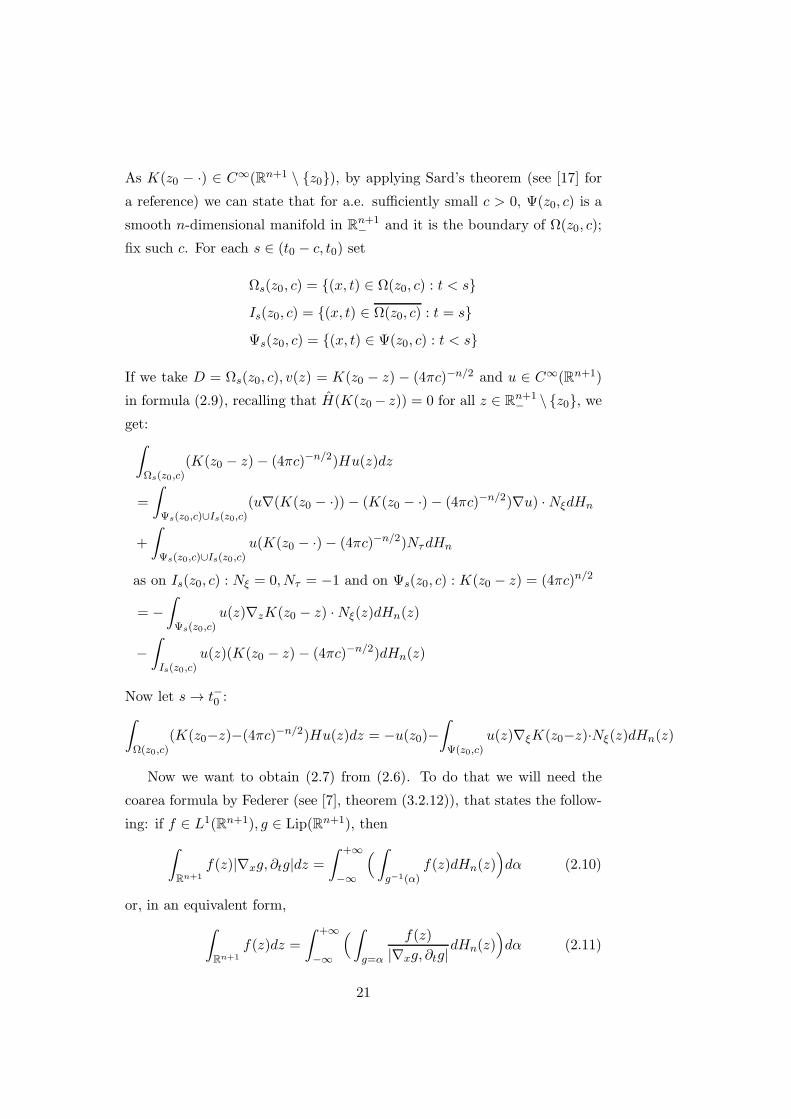
As K(z0 − ·) ∈ C∞(Rn+1 \ z0), by applying Sard’s theorem (see [17] for

a reference) we can state that for a.e. sufficiently small c > 0, Ψ(z0, c) is a

smooth n-dimensional manifold in Rn+1− and it is the boundary of Ω(z0, c);

fix such c. For each s ∈ (t0 − c, t0) set

Ωs(z0, c) = (x, t) ∈ Ω(z0, c) : t < sIs(z0, c) = (x, t) ∈ Ω(z0, c) : t = sΨs(z0, c) = (x, t) ∈ Ψ(z0, c) : t < s

If we take D = Ωs(z0, c), v(z) = K(z0 − z) − (4πc)−n/2 and u ∈ C∞(Rn+1)

in formula (2.9), recalling that H(K(z0 − z)) = 0 for all z ∈ Rn+1− \ z0, we

get:ˆ

Ωs(z0,c)(K(z0 − z)− (4πc)−n/2)Hu(z)dz

=

ˆ

Ψs(z0,c)∪Is(z0,c)(u∇(K(z0 − ·))− (K(z0 − ·)− (4πc)−n/2)∇u) ·NξdHn

+

ˆ

Ψs(z0,c)∪Is(z0,c)u(K(z0 − ·)− (4πc)−n/2)NτdHn

as on Is(z0, c) : Nξ = 0, Nτ = −1 and on Ψs(z0, c) : K(z0 − z) = (4πc)n/2

= −ˆ

Ψs(z0,c)u(z)∇zK(z0 − z) ·Nξ(z)dHn(z)

−ˆ

Is(z0,c)u(z)(K(z0 − z)− (4πc)−n/2)dHn(z)

Now let s → t−0 :

ˆ

Ω(z0,c)(K(z0−z)−(4πc)−n/2)Hu(z)dz = −u(z0)−

ˆ

Ψ(z0,c)u(z)∇ξK(z0−z)·Nξ(z)dHn(z)

Now we want to obtain (2.7) from (2.6). To do that we will need the

coarea formula by Federer (see [7], theorem (3.2.12)), that states the follow-

ing: if f ∈ L1(Rn+1), g ∈ Lip(Rn+1), then

ˆ

Rn+1

f(z)|∇xg, ∂tg|dz =

ˆ +∞

−∞

( ˆ

g−1(α)f(z)dHn(z)

)dα (2.10)

or, in an equivalent form,

ˆ

Rn+1

f(z)dz =

ˆ +∞

−∞

(ˆ

g=α

f(z)

|∇xg, ∂tg|dHn(z)

)dα (2.11)

21

Now take (2.6), multiply both sides by l−1+n/2 and integrate between 0 and

c:

ˆ c

0ln/2

ˆ

K=(4πl)n/2

u(ζ)(∇ζK(z0 − ζ)) · −→N ξ(ζ)dHn(ζ)dl

l

=2

nu(z0)c

n/2 +

ˆ c

0ln/2

ˆ

K>(4πl)n/2Hu(z)(K(z0 − z)− (4πc)−n/2)dz

dl

l

(2.12)

where we denote by K = (4πl)n/2 and K > (4πl)n/2 the sets Ψ(z0, c) and

Ω(z0, c) respectively. We would like to apply (2.11) to the left-hand side:

set α = (4πl)−n/2; then dα = −n

2

dl

l(4πl)−n/2. Putting this in (2.12) and

applying the coarea formula:

ˆ c

0ln/2

ˆ

K=(4πl)n/2

u(ζ)(∇ζK(z0 − ζ)) · −→N ξ(ζ)dHn(ζ)dl

l

=2

n

( 1

4π

)n/2ˆ ∞

(4πc)−n/2

1

α2

ˆ

K=αu(ζ)

|∇ζK(z0 − ζ)|2|∇xK(z0 − ζ), ∂tK(z0 − ζ)|dHn(ζ)dα

=2

n

( 1

4π

)n/2ˆ

K>(4πc)−n/2u(z)

|x0 − x|24(t0 − t)2

dz

By putting this last form in (2.12) we prove the thesis.

We are not ready to state one of the main results of this chapter; indeed,

the proof of the Wiener’s criterion for the heat equation is mainly based on

two lemmas: the following and one strong Harnack inequality that we will

show later.

Lemma 2.4.2. If u : Rn+1 → R is smooth, then

(i) the average

φ(c) =1

cn/2

ˆ

Ω(c)u(x, t)

|x|2t2

dxdt

is differentiable for c > 0.

(ii) Explicitly:

φ′(c) =n

2c(n+2)/2

ˆ

Ω(c)Hu(x, t)

Rc(t)2 − |x|2t

dxdt c > 0

22

(iii) There exists C1 > 0 that only depends on n such that if Hu ≤ 0 in

Ω(2c), c > 0 then

φ(2c) − φ(c) ≥ C1

cn/2

ˆ

Ω(c/2)(−Hu(x, t))dxdt

Proof. If we consider the change of variable (x, t)D7→ (

√cx, ct), we notice

that D(Ω(c)) = Ω(1) and hence:

φ(c) =1

cn/2

ˆ

Ω(1)u(√cξ, cτ)

1

c

|ξ|2τ2

c1+n/2dξdτ =

ˆ

Ω(1)u(√cξ, cτ)

|ξ|2τ2

dξdτ

By applying theorem (2.3.3) to the temperature v = 1 (with z0 = 0) one

sees that

ˆ

Ω(1)

|ξ|2τ2

dξdτ = 2n+2πn/2; by this and the fact that u is smooth

on Rn+1 and Ω(1) is compact, we know the integrand function is integrable

on Ω(1) with respect to variable (ξ, τ), hence we can differentiate under the

sign of integral. Notice that φ(c) = 4(4π)n/2uc(0); if we differentiate (2.7)

with respect to c we get:

duc(0)

dc= −

(n2

)2c−1−n/2

ˆ c

0ln/2

ˆ

Ω(l)Hu(z)(K(−z) − (4πl)−n/2)dz

dl

l

+n

2c

ˆ

Ω(c)Hu(z)(K(−z) − (4πc)−n/2)dz (2.13)

By Tonelli’s theorem one has

ˆ c

0ln/2

ˆ

Ω(l)Hu(z)(K(−z) − (4πl)−n/2)dz

dl

l

=

ˆ

Ω(c)Hu(z)

ˆ c

((4π)n/2K(−z))−2/n

ln/2(K(−z)− (4πl)−n/2)dl

ldz

=

ˆ

Ω(c)Hu(z)

[K(−z)

2

nln/2 − 1

(4π)n/2log l

]l=c

l=((4π)n/2K(−z))−2/ndz

=2

ncn/2

ˆ

Ω(c)Hu(z)K(−z)dz − 2

n(4π)n/2

ˆ

Ω(c)Hu(z)dz

− 2

n(4π)n/2

ˆ

Ω(c)Hu(z) log((4πc)n/2K(−z))dz (2.14)

By putting this in (2.13) we finally get:

1

4(4πc)n/2φ′(c) =

duc(0)

dc=

n

2c(4πc)−n/2

ˆ

Ω(c)Hu(z)

Rc(t)2 − |x|24t

dz

23

We just need to prove (iii): assume Hu ≤ 0 in Ω(2c). Hence

φ(2c)−φ(c) =

ˆ 2c

cφ′(s)ds =

n

2

ˆ 2c

c

1

s1+n/2

ˆ

Ω(s)(−Hu(z))

Rs(t)2 − |x|2−t

dzds

As the integrand function is positive and Ω(c/2) ⊂ Ω(c) ⊂ Ω(s), we get

φ(2c) − φ(c) ≥ n

2

ˆ 2c

c

1

s1+n/2

ˆ

Ω(c/2)(−Hu(z))

Rc(t)2 − |x|2−t

dzds

≥ n

2

ˆ 2c

c

1

s1+n/2

ˆ

Ω(c/2)(−Hu(z))

Rc(t)2 −R c

2(t)2

−tdzds

By simple calculation one can see thatRc(t)

2 −R c2(t)2

−t= 2n log 2, therefore:

φ(2c) − φ(c) ≥ n

2(2n log 2)

1

(2c)n/2

(ˆ

Ω(c/2)(−Hu(z))dz

)( ˆ 2c

c

1

sds)

=C1

cn/2

ˆ

Ω(c/2)(−Hu(z))dz

Before going further, it is useful to remind the classical Harnack inequal-

ity for the heat equation, for which one can refer to [3].

Theorem 2.4.3 (Pini-Hadamard). Let

ρ > ρ′ > 0

t1 > t2 > t3 > t4 > 0

and set

R = (x, t) : |xj | < ρ, j = 1, · · · , n, 0 < t < t1R− = (x, t) : |xj | < ρ′, j = 1, · · · , n, t4 < t < t3R+ = (x, t) : |xj | < ρ′, j = 1, · · · , n, t2 < t < t1

Then there is a positive constant C such that, for every non-negative tem-

perature u on R, one has:

supR−

u ≤ C infR+

u

24

Figure 2.2: Proof of lemma (2.4.4): the cylinders C,C ′.

Now set

Q(c) := (x, t) ∈ Ω(c) : −3

4c < t =

(x, t) : −3

4c < t < 0, |x|2 < 2nt log

(− t

c

)

We are now ready to state the other important result that will be crucial

for the final proof.

Lemma 2.4.4 (strong Harnack inequality). [Evans - Gariepy] Let u ≥ 0 a

solution of Hu = 0 in Q(2c), c > 0 and suppose u ∈ C(∂Q(2c) − 0); thenthere exists a constant C2 > 0, depending only on n, such that

|x|2≤ 3nc4

u(x,−3c

2

)dx ≤ C2 inf

Ω(3c/4)u (2.15)

(hereffl

denotes the n-dimensional integral average.)

Proof. Consider the change of variable (x, t)D7→

( x√c,t

c

). Then D(Q(1)) =

Q(c) and if u is such that Hu = 0 in Q(2), then H(u D) = 0 in D(Q(2)) =

Q(2c). The conclusion is unchanged over the mapping D, therefore it is

25

enough to prove the theorem in the case c = 1. Thanks to homogeneity it

is not restrictive to assume

|x|2≤ 3n4

u(x,−3

2

)dx = 1 (2.16)

We will prove that there is C2 as in the statement, so that 1 ≤ C2 infΩ(3/4)

u.

The proof is divided in two parts: at first we estimate infΩ(3/4) u on P ∩Ω(1),where P is a paraboloid we will build, using the classical Harnack inequality,

then we find a lower bound in Ω(1) \P by building a particular subsolution

v and using the maximum principle on u/v.

Consider at first the cylinder C ⊂ Q(2):

C := (x, t) : −3

2< t < −1, |x|2 < −3n log(3/4)

We can state there exists a constant α1 > 0 so that

u(x, t) ≥ α1 > 0 (x, t) ∈ C ′

C ′ = (x, t) : −5

4< t < −1, |x|2 ≤ 3n

4 ⊂ C

In fact, suppose this last statement is not true and that there is one point

z′ = (x′, t′) ∈ C ′ such that u(z′) = 0; thanks to Nierenberg maximum prin-

ciple we know u = 0 on C ∩ (x, t) : t ≤ t′. This would be a contradiction

of the assumption (2.16).

In the very same way, one can conclude there is α2 > 0 so that

u(x, t) ≥ α2 > 0 (x, t) ∈ D := Ω(1) ∩(x, t) : t < − 1

2e8

(2.17)

By theorem (2.3.3), for any (x, t) ∈ L := (0, t) : −1 < t < 0, one can

write:

u(0, t) =1

4πn/2

ˆ

Ω((0,t),1/4)u(x, s)

|x|2(t− s)2

dxds

and since for any t ∈(− 1

2e8, 0), the Lebesgue measure of D∩Ω((0, t), 1/4)

is strictly positive, by (2.17) we have

u(0, t) ≥ α3 > 0 (0, t) ∈ L

Define the truncated paraboloids:

P1 =(x, t) : |x|2 < −8nt,− 1

e8< t < 0

P2 =(x, t) : |x|2 < −16nt,− 1

e8< t < 0

26

Figure 2.3: Proof of lemma (2.4.4): the paraboloids and the cylinders.

As 2nt log(−t) = −16nt just for t = 0, t = −e−8, we can conclude P1 ⊂P2 ⊂ Ω(1).

Denote by S the closed cylinder

S := (x, t) : −b ≤ t ≤ −a, |x|2 ≤ c

with a, b, c > 0 such that1

2e8< a < b <

1

e8and

P1 ∩ (x, t) : −b ≤ t ≤ −a ⊂ (x, t) : |x|2 ≤ d,−b ≤ t ≤ −a⊂ S ⊂ P2 ∩ (x, t) : −b ≤ t ≤ −a

for some d ∈ (0, c)(see figure 2.4.4). Now call h := b− a > 0 and set

S+ =(x, t) : −a− 3

8h ≤ t ≤ −a− 1

8h, |x|2 ≤ d

⊂ S

S− =(x, t) : −a− 7

8h ≤ t ≤ −a− 5

8h, |x|2 ≤ d

⊂ S

Theorem (2.4.3) tells us that there exists C3 > 0 so that

maxS−

u ≤ C3minS+

u

27

The constant C3 does not change under the dilatation (x, t) 7→ (λx, λ2t), λ >

0, hence:

maxλS−

u ≤ C3minλS+

u 0 < λ ≤ 1

But for 0 < λ ≤ 1 one has L∩λS− 6= ∅ and by what we have proved before:

α3 ≤ C3minλS+

u 0 < λ ≤ 1 (2.18)

For any (x′, t′) ∈ P1 ∩(x, t) : − 1

2e8< t < 0

there exists λ ∈ (0, 1] so

that (x′, t′) ∈ λS+, so by (2.18) one has u(x′, t′) ≥ α3

C3. By putting this last

remark together with (2.17) we get

u(x′, t′) ≥ α4 > 0 (x′, t′) ∈ (x, t) ∈ Ω(1), |x|2 ≤ −8nt (2.19)

Now we need an estimate on W := Ω(1) \ (x, t) ≤ −8nt to complete

the proof. Consider the function ϕ : R+ → R, ϕ(x) = arctan(x + 16) −arctan(16); then for any x > 0:

ϕ(0) = 0

0 < ϕ(x) <π

2

ϕ′(x) > 0

0 ≤ −ϕ′′(x) ≤ 1

8ϕ′(x)

The last inequality comes from the following fact: call x+16 = t(⇒ t ≥ 16)

and differentiate:

ϕ′(x) =1

1 + t2− ϕ′′(x) =

2t

(1 + t2)2

One has to prove2t

1 + t2≤ 1

8⇔ t2 − 16t + 1 ≥ 0 and this is always true

when t ≥ 16. Now we can build the subsolution v as we anticipated at the

beginning of this proof:

v(x, t) = ϕ( |x|2

t− 2n log(−t)

)(x, t) ∈ Ω(1) (2.20)

Claim: Hv ≤ 0 on W .

28

Hv =(− |x|2

t2− 4n

t

)ϕ′ − 4|x|2

t2ϕ′′

≤(− |x|2

t2− 4n

t+

1

8

4|x|2t2

)ϕ′

=(− |x|2

2t2− 4n

t

)ϕ′ ≤ 0

since |x|2 ≥ −8nt in W . As ϕ(0) = 0, we have that

v = 0 on ∂Ω(1) \ 0

and

v ≤ π

2on (x, t) : |x|2 = −8nt

This and (2.19) imply

u

v≥ 2α4

π=: α on (x, t) : |x|2 = −8nt

and by maximum principle we can say

u ≥ αv on all W (2.21)

Now let Ω(3/4) ∩W and use the monotonicity of ϕ:

v(x, t) = ϕ( |x|2

t− 2n log(−t)

) t<0≥ ϕ

(2nt log(−4t/3)

t− 2n log(−t)

)

= ϕ(2n log

(43

))=: β > 0

Putting this last inequality, (2.17) and (2.21) we get:

u(x, t) ≥ maxα4, αβ

> 0 (x, t) ∈ Ω(3/4)

and this proves the assertion.

2.5 Necessity of (2.4)

This part of the proof is taken from Lanconelli’s work (see [11]). Assume

∞∑

k=1

2kn/2 capH(Ωc ∩A(2−k)) < ∞

29

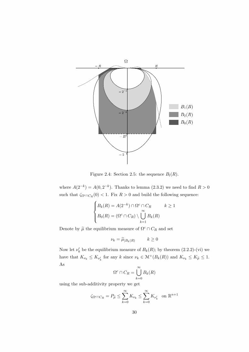
Figure 2.4: Section 2.5: the sequence Bl(R).

where A(2−k) = A(0, 2−k). Thanks to lemma (2.3.2) we need to find R > 0

such that ζΩc∩CR(0) < 1. Fix R > 0 and build the following sequence:

Bk(R) = A(2−k) ∩ Ωc ∩CR k ≥ 1

B0(R) = (Ωc ∩ CR) \∞⋃

k=1

Bk(R)

Denote by µ the equilibrium measure of Ωc ∩ CR and set

νk = µ|Bk(R) k ≥ 0

Now let ν ′k be the equilibrium measure of Bk(R); by theorem (2.2.2)-(vi) we

have that Kνk ≤ Kν′kfor any k since νk ∈ M

+(Bk(R)) and Kνk ≤ Kµ ≤ 1.

As

Ωc ∩CR =

∞⋃

k=0

Bk(R)

using the sub-additivity property we get

ζΩc∩CR= Pµ ≤

∞∑

k=0

Kνk ≤∞∑

k=0

Kν′kon R

n+1

30

In particular

Kν′k(0) =

ˆ

Rn+1

K(−z)dν ′k(z) =

ˆ

Bk(R)K(−z)dν ′k(z) (Bk(R) ⊂ A(2−k))

≤( 2k

2π

)n/2ν ′k(Bk(R)) =

( 2k

2π

)n/2capH(Bk(R))

Putting the last two remarks together we get

ζΩc∩CR(0) ≤ 1

(2π)n/2

∞∑

k=0

2kn/2 capH(Bk(R))

≤ 1

(2π)n/2capH(CR) +

1

(2π)n/2

∞∑

k=1

2kn/2 capH(Ωc ∩A(2−k) ∩ CR)

=: c(R)hyp.< ∞

As c(R) is increasing, by properties of the thermal capacity we can find R

so that c(R) < 1.

2.6 Sufficiency of (2.4)

The proof of the sufficiency was firstly given by L. C. Evans and R. F.

Gariepy (see [4]) in 1982. The proof is divided in several parts and strongly

relies on the strong Harnack inequality we showed before (theorem (2.4.4))

and on the average formulas of lemma (2.4.2) as we will soon see; this proof

was completed in details also following the work of N. Garofalo and E.

Lanconelli (see [8]).

Suppose that∞∑

k=1

2kn/2 capH(Ωc ∩A(2−k)) = +∞ (2.22)

We want to prove 0 is a regular point for Ω.

Modification of Ω.

Thanks to (2.22) we know at least one of the following four series diverges:

∞∑

k=1

2n2(4k+j) capH(Ωc ∩A(2−(4k+j))) j = 0, 1, 2, 3

therefore it is not restrictive to assume

∞∑

k=1

22kn capH(Ωc ∩A(2−4k)) = +∞ (2.23)

31

Figure 2.5: Section 2.6: modification of Ω.

32

By sub-additivity for any ǫ:

capH(Ωc ∩A(2−4k)) ≤ capH(Ωc ∩A(2−4k) ∩ (x, t) : t ≤ −ǫ)+ capH(Ωc ∩A(2−4k) ∩ (x, t) : −ǫ ≤ t ≤ 0) (2.24)

By lemma (2.2.1)-(v),(viii) we can say

limǫ↓0

capH(Ωc ∩A(2−4k) ∩ (x, t) : −ǫ ≤ t ≤ 0)

≤ limǫ↓0

capH(A(2−4k) ∩ (x, t) : −ǫ ≤ t ≤ 0) = capH(0) = 0

hence by (2.22) there exist a subsequence ǫll so that

∞∑

l=1

22ln capH(Ωc ∩A(2−4l) ∩ (x, t) : t ≤ −ǫl) = +∞ (2.25)

Define

Ωc = 0 ∪( ∞⋃

l=1

Ωc ∩A(2−4l) ∩ (x, t) : t ≤ −ǫl))∪ (Ωc \ Ω(1))

Then Ω ⊂ Ω, Ω is bounded and 0 ∈ ∂Ω. If 0 is a regular point for Ω, it is

regular also for Ω; in view of this, we can assume Ω = Ω; hence we can say

Ωc = 0 ∪( ∞⋃

l=0

Bl

)

where Bl ⊂ A(2−4l) ∩ (x, t) : t ≤ −ǫl l = 1, 2, · · ·

Ω(1) ⊂ Bc0 Bc

0 bounded

and∞∑

l=0

22nl capH(Bl) = +∞

Approximation.

The aim of this part is to regularize some equilibrium potentials; fix R > 0

and consider the compact set F = Ωc ∩ CR. Let ζF denote its equilibrium

potential and define

u := 1− ζF

33

Thanks to the arbitrary choice of R, we need to prove u(0) = 0 to apply

(2.3.2) and state that 0 is regular for Ω. Observe that by theorem (2.2.2):

0 ≤ u ≤ 1

u is a subtemperature on Rn+1 and a temperature on Ω

Hu = −µ in the sense of distributions

where µ is the equilibrium measure of F .

For each ǫ > 0 choose a compact set F ǫ so that

F ǫ = 0 ∪( ∞⋃

l=1

Bǫl

)⊂ CR+1

where

Bǫl is compact ǫ > 0, l = 1, 2, · · ·

Bl ∩ CR ⊂ int(Bǫl )

Bǫl ⊂ Ω(2−4l+1) \Ω(2−4l−2)

F ǫ ⊂ F ǫ′ if 0 < ǫ < ǫ′

F =⋂

ǫ>0

F ǫ

Denote by uǫ = 1 − ζǫ, where ζǫ is the equilibrium potential of F ǫ. Claim:

uǫ(z) ↑ u(z) := 1 − ηF (z) for ǫ ↓ 0, z 6= 0 As Fǫ′ ⊂ Fǫ for ǫ′ < ǫ, we

have Φǫ′ ⊂ Φǫ (see lemma (2.2.1)-(iii)), hence ηǫ′ ≤ ηǫ and consequently

ζǫ′ ≤ ζǫ; this monotonicity guarantees the existence of ξ(z) := limǫ→0

ζǫ(z)

for any z ∈ Rn+1. As F ⊂ Fǫ for any ǫ, we also have ζF ≤ ηǫ. Recall

(theorem (2.2.2)) that ζF = ηF on (∂F )c and ηF = 1 = ζǫ on F \ 0 as

F \ 0 ⊂ int(Fǫ). This forces ηF ≤ ζǫ except possibly at 0, hence

ηF ≤ ξ on Rn+1

On the other hand, ξ is a temperature on F c, 0 ≤ ξ ≤ 1 and lim|z|→+∞

ξ(z) = 0,

hence the weak maximum principle for supertemperatures (see for example

[18]) implies ξ ≤ v for any v ∈ ΦF , thus ξ ≤ ηF . Concluding, ξ = ηF on

Rn+1 \ 0.

As Bl ⊂ A(2−4l) ⊂ Ω(2−4l) for any l and the sequence Ω(2−4l)l is decreas-ing, we can find N = N(R) so that Bl ⊂ CR for all l ≥ N ; fix such l and call

34

ζ, µ respectively the backwards equilibrium potential and the correspond-

ing equilibrium measure for Bl (hence µ ∈ M+(Bl),Hζ = µ, capH(Bl) =

µ(Rn+1)).

Now we will realize what we anticipated at the beginning of this part and ap-

proximate ζ and uǫ by smooth functions. Pick the usual ϕ ∈ C∞0 (Rn+1), 0 ≤

ϕ ≤ 1,

ˆ

Rn+1

ϕ(z)dz = 1 and define

ϕδ =1

δn+1ϕ(zδ

)δ > 0

Set for any δ > 0

uǫδ = ϕδ ∗ uǫ

ζδ = ϕδ ∗ ζ

uǫδ and ζδ are smooth, nonnegative and bounded above by 1; moreover,

Huǫδ = H(ϕδ ∗ uǫ) = ϕδ ∗Huǫ = ϕδ ∗ (−µǫ) ≤ 0.

If we define a measure on Borel sets by µδ(A) =

ˆ

AHζδ(z)dz (H = −∆−∂t

is the backwards heat operator), we notice that it converges weakly to µ for

δ ↓ 0.

Now set c := 2−4l+1 for simplicity; we know by the previous part that

Bl ⊂ A(c/2), Bǫl ⊂ Ω(c) \ Ω(c/8)

If we take δ to be small enough we can have

supp µδ ⊂ int(Bǫl ) ∩ Ω

(34c)

uǫδ = 0 on supp µδ

as uǫ = 0 on int(Bǫl ). To apply lemma (2.4.4) we need to write uǫδ = vǫδ −wǫ

δ

where Hvǫδ = 0 on Q(2c)

vǫδ = uǫδ on ∂Q(2c) \ 0Hwǫ

δ = −Huǫδ ≥ 0 on Q(2c)

wǫδ = 0 on ∂Q(2c) \ 0

35

Estimates.

By direct calculation we are going to get an useful estimate:

( infΩ(3c/4)

vǫδ)2µδ

(Ω(34c))

≤ˆ

Ω(3c/4)(vǫδ)

2dµδ

Ω(3c/4)⊂Q(2c)

≤ˆ

Q(2c)(vǫδ)

2dµδ

=

ˆ

Q(2c)(wǫ

δ)2dµδ (as for small enough δ, uǫδ = 0 on supp µδ)

=

ˆ

Q(2c)(wǫ

δ(z))2(Hζδ(z))dz

=

ˆ

Q(2c)H(wǫ

δ(z))2ζδ(z)dz (because wǫ

δ = 0 on ∂Ω \ 0)

2

ˆ

Q(2c)wǫδ(z)(Hwǫ

δ(z))ζδ(z)dz − 2

ˆ

Q(2c)ζδ(z)|Dwǫ

δ(z)|2dz

wǫδ ζδ∈C

∞

≤ C

ˆ

Q(2c)(−Huǫδ(z))dz (as

ˆ

Q(2c)ζδ(z)|Dwǫ

δ(z)|2dz ≥ 0)

Q(2c)⊂Ω(2c)

≤ C

ˆ

Ω(2c)(−Huǫδ(z))dz

Summing up

( infΩ(3c/4)

vǫδ)2µδ

(Ω(34c))

≤ C

ˆ

Ω(2c)(−Huǫδ(z))dz

for small δ. By applying lemma (2.4.4) and (2.4.2)-(iii) we get

1

cn/2

(

|x|2≤3nc/4uǫδ

(x,−3

2c)dx

)2µδ

(Ω(34c))

≤ C(φ(uǫδ, 8c) − φ(uǫδ, 4c))

(2.26)

where

φ(f, s) =1

sn/2

ˆ

Ω(s)f(x, t)

|x|2t2

dxdt

Passage to limits.

Remember that

µδweak−→ µ

supp µδ ⊂ Ω(3c/4)

uǫδδ→0−→ uǫ pointwise a.e. and uniformly on compact subsets of (F ǫ)c

Hence

µδ

(Ω(34c))

= µδ(Rn+1)

δ→0−→ µ(Rn+1) = capH(Bl)

36

From (2.26) we get

1

cn/2

(

|x|2≤3nc/4uǫ(x,−3

2c)dx

)2capH(Bl) ≤ C(φ(uǫ, 8c) − φ(uǫ, 4c))

and letting ǫ ↓ 0

1

cn/2

(

|x|2≤3nc/4u(x,−3

2c)dx

)2capH(Bl) ≤ C(φ(u, 8c) − φ(u, 4c)) (2.27)

as u = u on F c. By lemma (2.4.2)-(iii), as Huǫδ ≤ 0, we have that

φ(uǫδ , 2jc)− φ(uǫδ, 2

j−1c) j = 0, 1, 2

By letting δ, ǫ ↓ 0 in the last expression, we get

φ(u, 2jc)− φ(u, 2j−1c) j = 0, 1, 2

As these are positive constants, we can modify (2.27) as follows

1

cn/2

(

|x|2≤3nc/4u(x,−3

2c)dx

)2capH(Bl) ≤ C

3∑

j=0

(φ(u, 2jc)− φ(u, 2j−1c))

Recalling that c = 2−4l+1, Bl ⊂ CR,∀l ≥ N and observing that the right

hand side is a telescopic series, we get

∑

l≥N

(βl)222nl capH(Bl) < ∞ (2.28)

where we have called

βl :=

|x|2≤3nc/4u(x,−3

2c)dx

therefore by (2.23) we can conclude

lim infl→∞

βl = 0 (2.29)

Estimates in cylinders.

Build the descreasing sequence of cylinders

Sl =(x, t) : |x|2 ≤ 3

2n2−4l, |t| ≤ 3 · 2−4l

l = 0, 1, · · ·

and set Ml := supSl

u and remember that 0 ≤ Ml ≤ 1; we want to prove

Mll→∞−→ 0.

37

Claim: there exist C4 > 0 and 0 < ν < 1 such that if Hv = 0 on S0, v is

continuous on the parabolic boundary ∂pS0 and 0 ≤ v ≤ M in S0, then

supS1

v ≤ νM + C4

|x|2≤nv(x,−3)dx (2.30)

Consider the representation of v in terms of the Green function for S0:

v(x, t) =

ˆ

|y|2≤3n/2G(x, t; y,−3)v(y,−3)dy

−ˆ 3

−3

ˆ

|y|2=3n/2

∂G

∂n(x, t; y, s)v(y, s)dHn−1yds

By taking v = 1 we notice that for any (x, t) ∈ S1:

ˆ

|y|2≤3n/2G(x, t; y,−3)dy −

ˆ 3

−3

ˆ

|y|2=3n/2

∂G

∂n(x, t; y, s)dHn−1yds = 1

(2.31)

Recall the properties of the Green function:

(i)∂G

∂n≤ 0

(ii) G ≥ 0

(iii) inf(x,t)∈S1,|y|2≤n

G(x, t; y,−3) ≥ γ > 0 for some γ

By these and (2.31), we get

0 <

ˆ

|y|2≤3n/2G(x, t; y,−3)dy < 1

0 < γ2 := −ˆ 3

−3

ˆ

|y|2=3n/2

∂G

∂n(x, t; y, s)dHn−1yds < 1

Call γ1 :=

ˆ

n<|y|2≤3n/2G(x, t; y,−3)dy; by property (iii) of G, there must be

ǫ > 0 so that γ1 < 1− ǫ. Hence for any (x, t) ∈ S1:

v(x, t) ≤ M

ˆ

n<|y|2≤3n/2G(x, t, y,−3)dy

+ sup|y|2≤n

G(x, t; y,−3)

ˆ

|y|2≤nv(y,−3)dy +Mγ2

≤ M(γ1 + γ2) + C4

ˆ

|y|2≤nv(y,−3)dy

= Mν + C4

ˆ

|y|2≤nv(y,−3)dy

38

The use the parabolic dilatation (x, t) 7→( x√

c,t

c

)allows us to conclude

that

supSl+1

v ≤ νMl + C4

|x|2≤n·2−4l

v(x,−3 · 2−4l)dx (2.32)

for any v such that Hv = 0, 0 ≤ v ≤ Ml in S0, v continuous on ∂pSl.

Now fix some number 0 < Θ < ν and fix Sl. Recalling who is βl and (2.29),

by using this last inequality one can state there is m > l such that

νMl + C4

|x|2≤n·2−4m

u(x,−3 · 2−4m)dx ≤ ΘMl (2.33)

Since u is bounded on Rn+1 there is a continuous function f defined on ∂pSl

so that

u ≤ f ≤ Ml on ∂pSl

with u = f on (x, t) : |x|2 ≤ n · 2−4m, t = −3 · 2−4m.Set v = HSm

f ; obviously v is a temperature and v ≤ f on ∂pSm, hence u ≤ v

on Sm. We have

Mm+1 = supSm+1

u ≤ supSm+1

v

(2.32)

≤ νMl +C4

|x|2≤n·2−4m

v(x,−3 · 2−4m)dx

v=HSmf

≤ νMl + C4

|x|2≤n·2−4m

f(x,−3 · 2−4m)dx

= νMl + C4

|x|2≤n·2−4m

u(x,−3 · 2−4m)dx =≤ ΘMl

Hence we have proved that for any l there exists m > l such that

Mm+1 ≤ ΘMl ≤ ΘMm

because Mjj is a decreasing sequence. As 0 < Θ < 1, the ratio test

guarantees us that

liml→∞

Ml = 0

Since u ≥ 0 and 0 =⋂

l≥0

Sl, this makes us conclude that u must be

continuous at 0 and u(0) = 1 − ζF (0) = 0, hence 0 is a regular point. The

proof is complete.

39

40

Further development

The Wiener’s criterion has been studied in more general settings than

the ones showed in this thesis; Garofalo and Lanconelli ([8]) proved it in the

case of a parabolic operator with variable coefficients and showed, as a main

consequence of it, that if L1, L2 are parabolic operators such that

Liu = div(Ai(x, t)∇u) − ∂tu

Ai real symmetric matrix-valued function on Rn+1 with C∞ entries

∃0 < µi ≤ 1 : µi|ξ|2 ≤n∑

i,j=1

aij(x, t)ξiξj ≤ µ−1i |ξ|2,∀ξ ∈ R

n

and Ω is a bounded open subset of Rn+1 and A1(z0) = A2(z0) for some

z0 ∈ ∂Ω, then z0 is L1-regular if and only if it is L2-regular.

Wiener’s test for regularity has recently been studied for the p-Laplacian

operator, defined by

∆pu = ∇ · (|∇u|p−2∇u) 1 < p < ∞

Moreover, Fabes, Garofalo and Lanconelli ([6]) proved the same results in

the case of parabolic operators with C1,α coefficients. Lanconelli went on

studying some sufficient and necessary conditions of regularity of boundary

points also in the case of parabolic operators with discontinuous coefficients

([12]); he underlined the fact that in the parabolic case it is not possibile to

find a representative operator, like in the elliptic case. In other words point

can be regular for the operator −a∆+ ∂t but not for −b∆+ ∂t (a > b > 0).

In 1994, Jan Maly and Tero Kilpelainen ([10]) proved the criterion for a

larger class of quasilinear partial differential operators that includes the p-

Laplacian for any p ≥ 1. The theorems is stated as follows: a finite boundary

41

point x0 ∈ ∂Ω(Ω ⊂ Rn) is regular if and only if

ˆ 1

0

(capp(B(x0, r) ∩ Ωc, B(x0, 2r))

capp(B(x0, r), B(x0, 2r))

) 1

p−1 dr

r= ∞

where capp is the p-capacity. Before them, Mazya found the proof of the

necessity for every p and Lindqvist and Martio managed to prove both ways

of the criterion in the case p > n− 1.

The criterion can be stated also in the setting of homogeneous Carnot groups

(see [2] for a reference) and takes the following form. Let G = (Rn, ⋆, δλ) be a

homogeneous Carnot group, L a sub-Laplacian on G and Γ its fundamental

solution with pole at 0. Let y ∈ G and E ⊂ G. Pick C > 1 and define the

anuli

Aj = x ∈ G : Cj ≤ Γ(y−1 ⋆ x) ≤ Cj+1

The following are equivalent:

(i) E is not L-thin at y.

(ii)

∞∑

j=1

Cj capL(Aj ∩ E) = ∞.

where we denote by capL(·) the capacity with respect to Γ, defined in a

similar way as for the Laplacian and the heat operator.

42

Bibliography

[1] D. H. Armitage, S. J. Gardiner, Classical potential theory, Springer,

2001.

[2] A. Bonfiglioli, E. Lanconelli, F. Uguzzoni, Stratified Lie groups and

potential theory for their sub-Laplacians, Springer, 2007.

[3] E. DiBenedetto, Partial differential equations, Springer, 2010.

[4] L. C. Evans, R. F. Gariepy, Wiener’s criterion for the heat equation,

Arch. Rational Mech. and Analysis, 78-4 (1982), 293-314.

[5] E. B. Fabes, N. Garofalo, Mean value properties of solutions to parabolic

equations with variable coefficients, Journ. Math. Analysis and Appl.,

121 (1987), 305-316.

[6] E. B. Fabes, N. Garofalo, E. Lanconelli,Wiener’s criterion for diver-

gence form parabolic operators with C1-Dini continuous coefficients,

Duke Math. J., 59 (1989), vol. 1, 191-232.

[7] H. Federer, Geometric measure theory, Springer-Verlag, 1969.

[8] N. Garofalo, E. Lanconelli, Wiener’s criterion for parabolic equations,

Trans. of the Am. Math. Soc., 308-2 (1988), 811-836.

[9] L. L. Helms, Introduction to potential theory, Wiley Interscience, 1969.

[10] J. Maly, T. Kilpelainen, The Wiener test and potential estimates for

quasilinear elliptic equations, Acta Math., 172 (1994), 137-161.

[11] E. Lanconeli, Sul problema di Dirichlet per l’equazione del calore, Ann.

Mat. Pura e Appl., IV, 97 (1973), 83-114.

43

[12] E. Lanconelli, Sul problema di Dirichlet per equazioni paraboliche del

secondo ordine a coefficienti discontinui, Ann. Mat. Pura e Appl., IV,

vol. CVI, 11-38.

[13] J. Moser, On a pointwise estimate for parabolic differential equations,

Comm. Pure Appl. Math., 24 (1971), 727-740.

[14] B. Pini, Sulle equazioni a derivate parziali, lineari del secondo ordine in

due variabili, di tipo parabolico, Ann. Mat. Pura Appl. (4), 32 (1951),

179-204.

[15] B. Pini, Sulla soluzione generalizzata di Wiener per il primo problema di

valori al contorno nel caso parabolico, Rend. Sem. Mat. Univ. Padova,

23 (1954), 422-434.

[16] B. Pini, Maggioranti e minoranti delle soluzioni delle equazioni

paraboliche, Ann. Mat. Pura e Appl. IV, 37 (1954), 422-434.

[17] S. Sternberg, Lectures on differential geometry, Prentice-Hall, Engle-

wood Cliffs, N.J., 1964.

[18] N. A. Watson, A theory of subtemperatures in several variables, Proc.

London Math. Soc., 26 (1973), 385-417.

[19] N. A. Watson, Green functions, potentials and the Dirichlet problem

for the heat equation, Proc. London Math. Soc., 33 (1976), 251-297;

Corrigendum, Proc. London Math. Soc., 37 (1978), 32-34.

[20] N. A. Watson, Thermal capacity, Proc. London Math. Soc., 37 (1978),

342-362.

[21] N. Wiener, The Dirichlet problem, J. Math. and Phys., 3 (1924), 127-

146.

44

Ringraziamenti

Il giorno della laurea e allo stesso tempo un inizio ed una fine; e per il

secondo suo aspetto che sento di dover rendere grazie a varie persone prima

di chiudere questo capitolo della mia vita. La mia famiglia e stata una

presenza costante nei miei anni di studi e li ha sostenuti economicamente,

non senza sacrifici; sebbene a volte ci siano state divergenze nei punti di

vista, non mi ha mai abbandonata. Questa tesi e dedicata ai miei genitori,

per il duro lavoro che intraprendono ogni giorno per crescere me e Marco.

Un enorme grazie spetta al mio compagno, Fabrizio, che non solo riesce a

sopportarmi e supportarmi quotidianamente, ma ha anche immediatamente

accettato di seguire me ed i miei sogni all’estero, lontano da tutto quello

che conosce. Risulta impossibile non nominare il professor Giorgio Guerrini,

la cui passione ed entusiasmo sono stati contagiosi per me fin dal primo

istante; e riuscito a farmi innamorare di quello che faccio e so che questo e

un raro privilegio. Come promesso, devo citare i passatelli di Maria Teresa,

fonte delle idee migliori! Ringrazio in generale tutta la famiglia Bugane, che

fin dai tempi del liceo mi ha trattata come una figlia. Sono perfettamente

consapevole della fortuna che ho ad avere nella mia vita cosı tante persone

che mi stimano, mi amano e mi sostengono, e non posso fare a meno di

essere loro riconoscente per cio che mi regalano.

45