The War on Illegal Drug Production and Trafficking:

An Economic Evaluation of Plan Colombia.∗

Daniel Mejıa† Pascual Restrepo‡

This version: June 2011

Abstract

This paper provides a thorough economic evaluation of the anti-drug policies im-

plemented in Colombia between 2000 and 2008, under Plan Colombia. We develop

a model of the war on drugs in which we explicitly model illegal drug markets. We

calibrate the model using available data and estimate important measures of the costs

and efficiency of different supply reduction policies in Colombia. We find that inter-

diction is more cost effective than eradication campaigns in reducing supply, and that

a three-fold increase in U.S. assistance would decrease the amount of cocaine in the

wholesale markets of transit countries by about 12.83%.

Keywords: Hard drugs, Conflict, War on Drugs, Plan Colombia.

JEL Classification Numbers: D74, K42.

∗The authors wish to thank Bruce Bagley, Jon Caulkins, Marcela Eslava, Andrew Foster, Hugo Nopo, Gerard Padro-i-

Miguel, Carlos Esteban Posada, Peter Reuter, Enrico Spolaore, Roberto Steiner, Rodrigo Suescun, Juan F. Vargas and Stephen

Walt for their valuable and detailed comments, as well as seminar participants at Berkeley, Brookings, Brown, Inter-American

Development Bank, ISSDP 2009, Lacea 2008, RAND, Stanford, Tufts, U.C. Irvine, U. de los Andes, U. del Rosario, U. of Miami,

U. of Warsaw, U. Torcuato Di Tella, the Colombian Ministry of Defense and the II NEAT workshop for useful discussions.

Maria Jose Uribe provided excellent research assistance. All remaining errors are ours. The first author acknowledges financial

support from Fedesarrollo’s “German Botero de los Rıos” 2008 Prize for Economic Research and the Open Society Institute.

†Corresponding author. Universidad de los Andes, e-mail: dmejia@uniandes.edu.co.

‡Universidad de los Andes, e-mail: p.restrepo23@uniandes.edu.co.

1

1 Introduction

In September 1999, the Colombian government announced a strategy known as Plan Colom-

bia, which aimed at (1) reducing the production of illegal drugs (primarily cocaine) by 50%

in six years; and (2) improving security in Colombia by reclaiming control of areas held by

armed groups (see the U.S. Government Accountability Office - GAO (2008)). Since 2000,

Plan Colombia has provided the institutional framework for the military alliance between

the U.S. and Colombia in the war against drug production, trafficking, and the organized

criminal groups associated with both.

During the last decade, the U.S. and the Colombian governments have allocated large

amounts of resources to the war on drugs in Colombia, where about 60% of the cocaine

consumed in the world is produced. According to the U.S. Government Accountability

Office (see GAO (2008)), between 2000 and 2008, the U.S. disbursed about $4.8 billion for

the military component of Plan Colombia; according to the Colombian National Planning

Department (see DNP (2006)), the Colombian government spent about $3.4 billion between

2000 and 2008. The joint expenditure per year on the military component of Plan Colombia

has been, on average, $1 billion, which corresponds to about 1.1% of Colombia’s yearly GDP

for this period.

Nevertheless, and despite the large amount of resources invested on the war on drugs since

2000, the results have been mixed. While the number of hectares of coca crops cultivated in

Colombia has decreased by about half (from 161,700 hectares for 1999 and 2000 to 86,000

hectares on average from 2005 to 2008), potential cocaine production has only decreased by

about 17% (from 689,000 kg per year for 1998,1999 and 2000, to 573,000 kg per year on

average from 2005 to 2008). This apparently paradoxical outcome can be explained by a

significant increase in yields per hectare, from about 4.3 kg of cocaine per hectare before 2000

to about 6.7 kg of cocaine per hectare per year from 2005 to 2008.1 Furthermore, consistent

with the observed patterns of potential cocaine production in Colombia, the wholesale price

1These increases in productivity have taken many different forms, among others, the use of stronger and

bigger coca plants, a higher density of coca plants per hectare, better planting techniques, and the use of

more efficient chemical precursors in the processing of coca leaf into cocaine.

2

of cocaine has remained relatively stable during these years.2

With the above stylized facts in mind, the general impression is that programs aimed

at reducing the production and trafficking of drugs have proved ineffective. For instance,

a recent report by the GAO recognizes that, although security in Colombia has improved

significantly during the current decade, the drug reduction goals of Plan Colombia were not

fully met (see GAO (2008)). However, little of a systematic nature is known about the

effects, costs and efficiency of the anti-drug policies implemented under Plan Colombia.3

The main objective of this paper is to fill this gap.

In this paper we construct a model of the war on drugs in producer countries. This war

takes place on two main fronts: those of production and trafficking. We explicitly model ille-

gal drug markets, which allows us to account for the feedback effects between policies, prices

and the main strategic responses of the involved actors, which are potentially important

when evaluating large-scale policy interventions such as Plan Colombia.4 We calibrate the

model using data from the war on drugs in Colombia, as well as the observed outcomes from

wholesale cocaine markets. Using the calibration results, we estimate different measures of

the costs and efficiency of the anti-drug policies implemented in Colombia between 2000 and

2008. Finally, we carry out simulation exercises, wherein we assess the effects of exogenous

changes in the U.S. budget allocated to Plan Colombia.

According to our estimates, the marginal cost to the U.S. of reducing the quantity of

2See Mejıa and Posada (2008) for a thorough description of the main stylized facts related to cocaine

markets, both in producer and consumer countries. Despite the recent intensification of the war on cocaine,

market prices at the wholesale and retail levels have remained relatively stable during the last seven years,

while consumption trends have not shown any decreasing tendency. See also the evidence cited in Caulkins

and Hao (2008), as well as the United Nations Office for Drug and Crime (UNODC) yearly reports.3Dube and Naidu (2009) explore a related question. In particular, they examine the impact of U.S.

military assistance on the intensity of conflict in Colombia. They find that U.S. military assistance in

Colombia has led to an increase in paramilitary attacks and has had no effect on the overall number of

guerrilla attacks.4Given our interest in evaluating current supply reduction policies in producer countries, our model stops

at wholesale markets in transit countries, and does not take into account seizures in these countries or other

anti-drug policies implemented in consumer countries. See Mejıa and Restrepo (2011) for a model that

studies the interactions between anti-drug policies in producer and consumer countries.

3

Colombian cocaine in transit countries by one kg is about $19,000, if the assistance is used

to subsidize eradication efforts in Colombia (e.g., the war with drug producers over the

control of arable land), whereas the marginal cost is about $7,800 if the assistance is used

to subsidize interdiction efforts (e.g., the war with drug traffickers over the control of the

routes used to transport illicit drug shipments). Consequently, if the U.S. government wants

to minimize the supply of Colombian cocaine, it should reallocate resources from eradication

to interdiction efforts. Doing so would reduce the amount of cocaine leaving Colombia

by 2.43% (i.e., by about 11,000 kg). Under this optimal allocation of subsidies (in terms

of supply reduction), the marginal cost to the U.S. of reducing the supply of Colombian

cocaine at transit countries by one kg would be about $12,300, either subsidizing interdiction

or eradication. Additionally, we estimate that a three-fold increase in U.S. assistance for

Plan Colombia (from about $593 million per year to $1.5 billion per year) would lead to

a reduction of about 12.8% (i.e., about 52,000 kg) in the amount of Colombian cocaine at

transit markets.

Although both the U.S. and Colombia have an interest in fighting the war on drugs under

the current prohibitionist regime, they do not necessarily agree in the preferred means for

doing so. This may be because they have different underlying objectives. For instance, if

the Colombian government’s objective is to minimize the total cost arising from the internal

conflict fueled by the drug business, as we assume in our model, Colombia may be worse off

under an optimal allocation of subsidies from a supply reduction perspective. According to

our estimations, this occurs because the Colombian government faces a larger net marginal

cost from illegal drug production activities (a net cost of about $0.32 for every dollar re-

ceived by drug producers) relative to the net marginal cost from drug trafficking activities

(a net cost of about $0.13 for every dollar received by drug traffickers). Consequently, the

Colombian government would prefer to see more U.S. subsidies allocated to the war against

drug producers, even if this comes at the expense of less subsidies for the war against drug

traffickers.

Finally, we identify the key aspects and economic forces behind the high (and different)

costs of eradication and interdiction policies in producer countries. The first factor is a

low price elasticity of the demand for drugs (as also identified by Becker, Murphy and

4

Grossman (2006)). The second factor relates to the strategic responses by drug producers

and traffickers to the specific types of anti-drug policies implemented, which counteract their

effectiveness. More precisely, producers and traffickers respond to higher prices by increasing

the productivity of land and routes respectively, creating an upward slopping supply at each

stage. Supply reduction policies become less effective because they raise prices, and supplied

quantities increase with higher prices. In our model, the participation in total product of

the stage being disrupted does not matter, as suggested by the so-called additive model.

Although policies aimed at disrupting upstream markets (in our case, interdiction) have a

larger impact on quantities, these interventions are more costly. This occurs because the

agents involved in these stages are willing to spend more money to avoid them, since the

size of the prize that they are fighting for is larger.

Most of the available literature on the effects of anti-drug policies has focused on partial

equilibrium analysis.5 However, the market for illegal drugs hides complex interactions

that should be addressed using models that can account for the feedback effects between

policies, prices, and the consequent strategic reactions of the actors involved, especially when

evaluating such large-scale policy interventions as Plan Colombia. Important exceptions

are Becker et al. (2006), Naranjo (2007), Chumacero (2008), Costa Storti and De Grauwe

(2009), and Mejıa and Restrepo (2011). These papers explicitly model illegal drug markets

when analyzing the effects of anti-drug policies. Becker et al. (2006) show how the social

costs of fighting against drugs crucially depends on the price elasticity of the demand for

drugs. In particular, they show that if the demand for drugs is highly inelastic, policies

aimed at reducing the supply of drugs by punishing dealers are socially optimal only when

the negative externalities associated with drug consumption are sufficiently high. Naranjo

(2007) develops a model in which insurgent groups provide security for drug producers in

5See Caulkins, Feichtinger and Tragler (2001) and Rydell, Caulkins and Everingham (1996) for partial

equilibrium studies on the trade-off between treatment versus enforcement policies in reducing the consump-

tion of illegal drugs. Grossman and Mejıa (2008) study the relative efficiency and effectiveness of eradication

and interdiction efforts in a partial equilibrium game theory model. For a thorough survey of the literature

on the effects of source country control interventions and the effects of treatment and prevention policies in

reducing the demand for illegal drugs in consumer countries, see Caulkins (2004), Reuter (2008), and Mejıa

and Posada (2008).

5

exchange for a fraction of the drug output. He finds that supply side interventions may

have a counter-productive effect on the drug industry and may increase conflict. Chumacero

(2008) focuses on the effects of three alternative anti-drug policies (making illegal activities

riskier, increasing the penalties to illegal activities, and legalization). Costa Storti and

De Grauwe (2009) and Mejıa and Restrepo (2011) focus on the interrelationship between

anti-drug policies aimed at reducing the demand for drugs (such as treatment and prevention

policies in consumer countries) and policies aimed at reducing the supply of drugs (by means

of interdiction and increased enforcement). Finally, Jeff Miron analyses the costs of drug

prohibition (Miron and Zwiebel (1995)) and the budgetary consequences of drug legalization

in the U.S. (Miron (2010)). However, none of these contributions focuses on evaluating the

costs, effectiveness and future prospects of the war on illegal drugs in producer countries,

nor are they aimed at evaluating actual anti-drug policies. This paper does both.

The rest of the paper is organized as follows: section 2 presents the model; section 3

contains the calibration strategy, results, as well as the results from the simulations; sec-

tion 4 discusses the key factors that tend to make the war against illegal drug production

and trafficking more costly/less effective and discusses the potential asymmetries between

Colombia and the U.S. in terms of the preferred strategy for the war on drugs; and section

5 concludes.

2 The Model

We model the war against drug production and trafficking as a sequential game in which

there are five actors involved: the government of the drug producing country (henceforth

the government); the government of the drug consumer country (henceforth the interested

outsider); a drug producer; a drug trafficker; and a wholesale dealer located outside the

borders of the producer country, at transit countries (an international drug trafficker). The

last one plays no active role other than demanding drugs from traffickers. The model builds

on previous work by Grossman and Mejıa (2008).

We explicitly model two drug markets: the production, or domestic market, and the

international wholesale market. In the domestic market, the producer sells illicit drugs, Qd,

6

at a price Pd to the drug trafficker. In the wholesale market, the trafficker sells the drugs

that survive interdiction efforts, Qf , at a price Pf to the international drug trafficker, who

is located along transit countries such as Mexico, in the case of Colombian cocaine going

to U.S. markets. Our model stops at the wholesale markets in transit countries, precisely

because the objective of our paper is to evaluate supply reduction policies in the source

countries, such as those implemented under Plan Colombia.

On the one hand, the war against production- the eradication front of the war on drugs-

is aimed at reducing the supply in the domestic market by targeting the land controlled by

producers and used, together with other factors, to produce drugs.6 On the other hand, the

war against trafficking- the interdiction front of the war on drugs- is aimed at reducing the

supply in the wholesale markets by targeting and blocking the routes used by traffickers to

transport drug shipments outside of the producer country.7

At each stage, we include a non-targeted production factor. For instance, producers use

other inputs such as gasoline, cement and sulfuric acid purchased in competitive markets

to process coca leaf into cocaine.8 When domestic prices increase, producers respond by

investing more in these factors, thus increasing the productivity of land under cultivation.

On the other hand, traffickers use drugs purchased in a competitive domestic market. When

wholesale international prices increase relative to domestic prices, traffickers respond by

buying more drugs to send through the routes they control, thus increasing the productivity

of drug routes. These strategic responses, arising from changes in prices, imply that both

the domestic and wholesale supply curves are upward sloping.

In order to rationalize the government’s incentives to fight the war on drugs, we assume

6The model is based on the Colombian case, where coca bushes are the raw material for producing cocaine.

However, the model also applies for other cases, for instance Afganisthan, where opium poppies are the raw

material for producing heroin.7We call these two policies eradication and interdiction for simplicity’s sake, but that does not mean that

we are giving them a narrow interpretation. For instance, eradication refers not only to the destruction of

illicit crops, but also to the prevention of their cultivation by expanding the state’s presence. In a similar

way, interdiction refers not only to the interception of drug shipments, but also to the prevention of drug

traffickers from using routes or sending shipments (for instance, by policing the country’s borders).8See Mejıa and Rico (2010) for a thorough description and quantification of the cocaine production process

in Colombia.

7

that it faces a net cost, c1 > 0, per unit of income obtained by the drug producer, and a

net cost, c2 > 0, per unit of income obtained by the drug trafficker.9 The intuition behind

this modeling assumption is that illegal groups engaged in the production and trafficking of

illicit drugs use part of the proceeds from these activities to finance terrorist attacks against

the government and civilians, corrupt politicians, weaken local institutions and the rule of

law, and so forth, whereas another fraction is used in other, perhaps legal, activities that

do not generate direct costs to the drug producing country’s government. Thus, c1 and c2

capture the net cost to the government arising from illegal drug production and trafficking

activities, respectively.10

Finally, we model Plan Colombia as a scheme in which the interested outsider grants

the government’s military forces two types of subsidies, in an attempt to strengthen their

resolve in the war against drug production and trafficking. These subsidies consist of a

fraction (1− ω) ∈ [0, 1) of the resources the government spends on the eradication front,

and a fraction (1− Ω) ∈ [0, 1) of the resources it spends on the interdiction front.

The timing of the game is as follows:

1. The interested outsider grants subsidies 1−ω and 1−Ω to strengthen the government’s

resolve to disrupt drug production and trafficking, respectively.

2. On the eradication front, the government engages the illegal drug producer in a conflict

over the control of arable land suitable for cultivating the crop necessary to produce

illegal drugs. Afterwards, the drug producer decides the amount of resources to invest

in factors complementary to land in the production of illegal drugs, such as chemical

9These costs need not be equal for many different reasons. For instance, drug producers, as is the case in

Colombia, finance terrorist activities against the government (at least in part) from the income receive from

illegal drug production activities. Drug traffickers, on the other hand, might use a different fraction of the

proceeds from illegal drug trafficking to corrupt politicians, bribe anti-narcotics police, and so forth.10Under the current prohibitionist regime, drug production and transportation are in the hands of illegal

armed groups and organized crime, most probably because these groups have a comparative advantage, as

they can enforce property rights and contracts by exerting violence. If production were legalized, one would

expect legal producers with lower production costs and operating at an optimal scale to take over these

activities.

8

precursors, workshops and other materials. At this stage, we obtain the domestic

supply, Qsd.

3. On the interdiction front, the government engages the drug trafficker in a conflict over

the control of the routes used to transport illegal drugs. Afterwards, the drug trafficker

decides the amount of illegal drugs to buy from the drug producer. At this stage, we

obtain the domestic demand for drugs in the producer country, Qdd.

4. In the last stage of the game, the drug trafficker offers the drugs successfully trafficked

to a wholesale international drug trafficker, located in transit countries. At this stage

of the game, we obtain the wholesale supply of drugs in transit countries, Qsf . The

drugs are sold to a dealer with a generic demand function Qdf .

We now turn to a description of each stage of the game described above. We briefly

describe the problem faced by each agent involved, their objective functions and restrictions,

and the production, conflict and trafficking technologies. We start with the last stage of the

game.

2.1 The international drug trafficker

In order to simplify the analysis that follows- and inasmuch as the main purpose of this

paper is to study the war on illegal drug production and trafficking in producer countries,

such as Colombia- we assume that the international drug trafficker’s demand for drugs is

given by a general demand function of the form11

Qdf =

a

P bf

. (1)

Here, Qdf denotes the demand for drugs by the international drug trafficker, a > 0 is a

scale parameter, Pf is the wholesale price in transit countries, and b is the price elasticity of

demand. In this paper, we do not consider what happens after the drugs are transported into

11See Mejıa and Restrepo (2011) for a model extending the framework developed in this paper by intro-

ducing the role of prevention and treatment policies in consumer countries aimed at reducing the demand

for drugs.

9

transit countries- that is, we do not model how the international drug trafficker transports

illegal drugs to consumer countries, or the effects of other anti-drug policies implemented in

transit and consumer countries.

2.2 The interdiction front

We assume that the drug trafficker combines routes, κ, with domestic drugs, Qd, to “produce”

drug shipments to transit countries, Qf . Thus, traffickers are modeled as intermediaries who

transport drugs from source to transit countries. We assume that only a fraction h ∈ [0, 1] of

the possible routes are not interdicted (or blocked) by the government. Formally, the drug

trafficking technology is given by

Qf = (κh)1−ηQηd, (2)

where η captures the relative importance of domestic drugs and 1− η captures the relative

importance of routes in the drug trafficking technology. κ is a scale parameter.12 The Cobb

Douglas functional form is inspired by the fact that routes are used multiple times to send

drug shipments, and each route has diminishing returns because it has a fixed capacity.

Although the Cobb Douglas assumption is necessary for our calibration and simulations,

one could also interpret our results locally by assuming that equation 2 is a log linear

approximation around the equilibrium. Moreover, we think of interdiction as an effort aimed

at disrupting trafficking routes, rather than simply seizing specific shipments, which have a

relative low cost for traffickers.

The interdiction technology is such that h, the fraction of routes that survive the gov-

ernment’s interdiction efforts, is determined endogenously by a standard context success

function (CSF) given by13

h =γt

γt+ s. (3)

12The constant returns to scale technology in equation 2 implies that, at the aggregate level, it does not

make any difference whether there is just one or many drug traffickers.13A contest success function (CSF) is a technology wherein some or all contenders for resources incur

costs as they attempt to weaken or disable competitors (see Hirshleifer (1991)). See Skaperdas (1996) and

Hirshleifer (2001) for a detailed explanation of the different functional forms of CSF.

10

Here, s denotes the resources allocated by the government to interdiction efforts (airplanes,

fast boats, etc), t denotes the resources that the drug trafficker invests in trying to avoid

interdiction (for instance, in submarines, fast boats, airplanes, pilots, drug mules, corrupting

government officials to avoid being captured, etc) and γ > 0 captures the relative effectiveness

of the trafficker’s resources invested in the conflict for routes.

The drug trafficker’s profits are given by:

πT = PfQf − PdQd − t. (4)

The first term in equation 4 is the total income from drug sales in wholesale international

markets in transit countries. The second term is the cost of the domestic drugs used for

trafficking. Finally, recall that t are the resources invested by the drug trafficker in trying

to avoid the government’s interdiction efforts.

The drug trafficker takes prices as given and maximize profits, πT . The trafficker first

chooses t with the government simultaneously choosing s, which determines the equilibrium

value for h. Afterwards, the trafficker chooses the domestic drugs, Qd, that will be intended

to be trafficked, based on the expectation of controlling a fraction h of the routes.

When determining the amount of resources allocated to interdiction efforts, the govern-

ment’s objective is to minimize the sum of the costs associated with illegal drug trafficking,

CT , where

CT = c2PfQf + Ωs. (5)

The trafficker’s income, PfQf , is multiplied by the net cost, c2, perceived by the govern-

ment for each unit of income received by the drug trafficker. The second term, Ωs, denotes

the cost to the government of fighting the war against drug trafficking. This cost is the share

of the resources allocated to the interdiction front that are paid by the government. Recall

that the remaining fraction, 1−Ω, of s is subsidized by the interested outsider. The govern-

ment chooses the amount of resources to invest in interdiction efforts, s, so as to minimize

CT , with the trafficker simultaneously choosing t. When doing so, it anticipates the drug

trafficker’s subsequent demand for drugs in the producer country, Qd, and takes Ω and prices

as given.

11

The Nash equilibrium for the drug trafficking sub-game is described by the following

equations:14

t∗ = (1− h∗)(1− η)PfQf , s∗ =c2Ω(1− h∗)PfQf , h∗ =

γΩ(1− η)

c2 + γΩ(1− η),

Qdd(Pd, Pf ) = h∗κ

(ηPfPd

) 11−η

and Qsf (Pd, Pf ) = h∗κ

(ηPfPd

) η1−η

.

(6)

2.3 The eradication front

We assume that the drug producer combines arable land, L, necessary for cultivating the il-

legal crop with other complementary resources (workshops, chemical precursors, microwaves,

labor, etc.), r, in order to produce drugs, Qd. We assume that only a fraction q ∈ [0, 1] of

the land potentially available for cultivation is used and not eradicated. We also consider

as ’eradicated’ all the land that is not used because of a strong state presence. Formally,

domestic drug production is given by

Qd = λ(qL)1−αrα (7)

where λ > 0 is a scale parameter, α and 1−α are the relative importance of the complemen-

tary factors and land respectively in the production of illicit drugs, and qL is the amount

of land the drug producer controls and which is not eradicated.15 Although the Cobb Dou-

glas assumption is necessary for our calibration and simulations, one could also interpret

our results locally by assuming that equation 7 is a log linear approximation around the

equilibrium.

The drug producer initially controls L hectares of land, which could potentially be used

to cultivate illegal crops. The eradication technology is such that q, the fraction of land with

coca crops that survives the eradication efforts, is determined endogenously by the following

14All the derivations are presented in the appendix, where we solve this sub game by backwards induction.

The order in which the trafficker and the government are assumed to play does not affect our results and we

solve it sequentially only because the algebra becomes easier. If all inputs were chosen simultaneously, then

we would have h∗ = γΩc2+γΩ

. Our results would be unaffected by this modeling choice since the calibrated

value of γ would adjust to recognize that the (1− η) factor is no longer there.15Again, the constant returns production technology in equation 7 implies that, at the aggregate level, it

does not make any difference whether there is just one or many drug producers.

12

contest success function:

q =φx

φx+ z, (8)

where z denotes the governments’ resources allocated to eradication efforts, such as aerial

spraying campaigns, manual eradication campaigns and, more generally, all government ef-

forts aimed at making sure that arable land is used for legal purposes; x are the resources

invested by the drug producer in trying to avoid eradication efforts, for instance, via insur-

gents and arms; finally, φ > 0 captures the relative effectiveness of the producer’s resources

allocated to this conflict.

The drug producer’s profits are given by:

πP = PdQd − r − x, (9)

The first term in equation 9 is the total income derived from drug production activities.

The second term, r, denotes the expenses on complementary factors. Finally, recall that

x denotes the resources invested by the drug producer in trying to avoid the government’s

eradication efforts.

The drug producer takes prices as given and maximize profits, πP . The producer first

chooses x with the government simultaneously choosing z, which determines the equilib-

rium value for q. Afterwards, the producer chooses complementary factors, r, based on the

expectation of controlling a fraction q of total land, L.

When determining the amount of resources allocated to eradication efforts, the govern-

ment objective is to minimize the sum of the costs associated with illegal drug production,

CP , where:

CP = c1PdQd + ωz. (10)

The producer’s income PdQd is multiplied by the net cost, c1, perceived by the government

from each unit of income received by the drug producer. The second term, ωz, denotes the

government expenses in the war against drug production. This cost is given by the share

of the resources allocated to the eradication front paid by the government. Recall that the

remaining fraction, 1 − ω, of z is paid by the interested outsider. The government chooses

the amount of resources to invest in eradication efforts, z, so as to minimize CP , with the

13

producer simultaneously choosing x. When doing so, it anticipates the drug producer’s

investment in complementary factors, r, and takes ω and prices as given.

The Nash equilibrium for the drug production sub-game is described by the following

equations:16

x∗ = (1− q∗)(1− α)PdQd, z∗ =c1ω(1− q∗)PdQd, q∗ =

φω(1− α)

c1 + φω(1− α),

r∗ = q∗α1

1−αλ1

1−αP1

1−α

d L and Qsd(Pd) = q∗α

α1−αλ

11−αP

α1−α

d L.

(11)

2.4 The drug market equilibrium

Equilibrium prices and quantities are given by the market clearance condition in domestic

and international markets. Equilibrium quantities are given by

Q∗

d = q∗b(1−α)

b+αη−bαηh∗−α(1−b)(1−η)b+αη−bαη K1 and Q∗

f = q∗bη(1−α)

b+αη−bαηh∗b(1−η)

b+αη−bαηK2 (12)

where K1 and K2 are constants, as specified in Appendix A.17

We can use these expressions to understand how eradication efforts (a lower q∗) or in-

terdiction efforts (a lower h∗) affect the equilibrium quantities of drugs transacted in the

domestic and international drug markets. To start, notice that both elasticities sum less

than 1, implying that the war on drugs has decreasing returns to scale, in the sense that

reducing q and h by half would reduce the supply at transit countries by less than half. Thus,

the original Plan Colombia objective of reducing cocaine supplied by Colombia in 50% would

require that q and h were reduced by more than 50%. the observed reduction in q of about

50% and in h of about 14%, from 2000 to 2008, was insufficient for reaching this objective.

The two elasticities depend on η(1−α) and (1−η), respectively, which is the participation

of the factors targeted at each of the fronts of the war on drugs. Thus, this equation suggests

16All the derivations are presented in the appendix. There, we solve this sub game by backwards induction.

Again, the order in which the producer and government are assumed to play does not affect our results and

we solve it sequentially only because the algebra is easier that way. If all inputs were chosen simultaneously,

then we would have q∗ = φωc1+φω

. Our results would be unaffected by this modeling strategy since the

calibrated value of φ would adjust to recognize that the (1− α) factor is no longer there.17The analytic solution for equilibrium prices P ∗

d and P ∗f ) is shown in Appendix A. Equilibrium prices

determine the value of all the other endogenous variables of the model.

14

that targeting the factors with the largest participation in final product has a greater impact

on quantities (in our case, this factor would be the routes). This argument is in line with

the “additive model” of the war on drugs. According to this view, interventions in source

countries are ineffective as the value of domestic drugs only accounts for a small share of

total income. However, traffickers and producers are willing to fight harder for these highly

valuable inputs, making it hard to conclude that policies should only be aimed at targeting

inputs with a bigger participation in total product. In other words, while disrupting the

“markets” of key inputs may be very effective, it is also very costly.

Both elasticities are smaller for small values of the demand elasticity, b. Thus, a lower

elasticity of demand implies weaker effects of supply reduction policies on final quantities,

as is the case in most analysis of drug markets. Finally, if the international demand for

drugs is inelastic, domestic equilibrium quantities increase with interdiction efforts, whereas

they always decrease with eradication efforts. The intuition behind the first result is that

interdiction raises the price of drugs at wholesale markets relative to domestic markets. This

compensates traffickers for the extra losses and motivates them to send more drugs, even

though a smaller fraction will be successfully trafficked.

2.5 Efficiency and the interested outsider’s problem

In order to study the costs and efficiency of supply reduction policies, we must first define

an objective function for the interested outsider. Thinking from the U.S. perspective, we

postulate supply reduction as a first order objective and a useful benchmark to evaluate the

anti-drug component of Plan Colombia (e.g., its first objective was to reduce the amount

of cocaine reaching U.S. markets by 50%). In particular, we assume that the interested

outsider’s (the U.S. government) problem is given by

minω,Ω

Q∗

f subject to: Mo = (1− ω)z∗ + (1− Ω)s∗ ≤M. (13)

Q∗

f denotes the equilibrium wholesale supply at transit countries and Mo the interested

outsider’s equilibrium expenditures. Let Q(M) be the value function of this optimization

problem. We call this the interested outsider’s problem, and it can be viewed as the first

stage of our game, wherein the interested outsider decides which subsidies to grant given

15

an exogenous budget for the war on drugs in producer countries. We treat M as exogenous

because we want to study how quantities (and other endogenous variables) react to exogenous

changes in this budget. We do not consider the welfare problem faced by the interested

outsider when determining the level of this budget.

We call a pair of subsidies optimal if it minimizes the quantities transacted in international

drug markets- that is, Q∗

f = Q(M) for a given budget level M . Although we recognize that

there might be other objectives from the interested outsider’s point of view, minimizing

the amount of drugs transacted in international markets is a first order objective and a

good starting point to estimate the costs and effectiveness of supply reduction policies.

Even if the interested outsider had a different objective function, this optimization problem

would still be useful, as it characterizes the feasible set of pairs (Qf ,M) : Qf ≥ Q(M) it

could induce- and therefore ’choose’- by subsidizing the producer country in the war against

production and trafficking. Thus, independently of its objective, the interested outsider

faces the technological constrain Qf ≥ Q(M). It is very likely that this restriction would be

binding, making it important to study this optimization problem.

In any internal solution, the optimality condition for the interested outsider’s problem

implies that the marginal cost of reducing Qf in one kg must be equal by subsidizing both

eradication or interdiction efforts.18

3 Calibration strategy and results

3.1 A brief description of the data used in the baseline scenario

In order to calibrate the parameters of the model, we use U.S. expenditure figures from

the General Accountability Office’s report to the U.S. Congress (GAO (2008)). This report

includes annual expenditures from 2000 to 2008 for each of the different cooperation programs

developed under Plan Colombia. Appendix C describes our methodology to approximate the

U.S. assistance to the eradication and interdiction fronts from this data. During the years

2000 to 2008, the U.S. spent about $4.75 billion (excluding the $115 million used for the

18Nevertheless, the two marginal costs need not be equal if the solution to the interested outsider’s problem

is a corner solution, with either ω∗ = 1 or Ω∗ = 1.

16

Infrastructure Security Strategy, a program aimed at protecting oil pipelines); out of this,

$3.26 billion was allocated to the eradication front and $1.48 billion to the interdiction front

according to our estimates. This division implies that about 69% of the budget allocated

by the U.S. to Plan Colombia was used for eradication efforts, while the remaining 31% was

used for interdiction efforts. These numbers imply an estimate for annual U.S. expenditures

on Plan Colombia of $593 million per year, out of which $408 million subsidized eradication

efforts, and the remaining $185 million subsidized interdiction efforts. We acknowledge that

our construction of these values may be subject to criticism, and only corresponds to an

educated guess. To address this concern, we check the robustness of our results by assuming

different values for the share of resources used to subsidize the eradication front (see the

robustness checks section in the Appendix).

[Insert Table A1 here: U.S. expenditures on Plan Colombia, 2000-2008.]

We also use drug markets’ outcomes time series.19 This data covers the years 1998-2008,

and includes prices at the wholesale level in the U.S., farm gate cocaine prices in Colombia,

the number of hectares of land with coca crops in Colombia, land productivity per year in

Colombia and cocaine seizures by Colombian authorities. All these series are taken from

UNODC yearly reports (see UNODC (2009)). For each variable, we define its value before

Plan Colombia as its average in the years 1998, 1999 and 2000, and its value after Plan

Colombia as its average for the years 2005, 2006, 2007 and 2008. The change over time in

some of the variables allows us to recover some of the structural parameters of the model.

We define the final price (Pf ) perceived by Colombian traffickers as one fourth of the

wholesale price in the U.S., which is consistent with the observed markups reported in Mejıa

and Rico (2010). By doing this, we obtain an international price of about $8.000 per kilogram

of cocaine, similar to the reported price of cocaine in Mexico and other transit countries.20

Importantly, we do not require a value for Pf before Plan Colombia in our calibration exercise.

Thus, we do not need to assume that the associated markups have not changed over time.

19For a thorough description of the available data on cocaine production, trafficking and drug markets, as

well as the collection methodologies and main biases in the data, see Mejıa and Posada (2008).20An online interview with the AUC’s former chief (Salvatore Mancuso) also suggests a

price level of this order of magnitude. The interview can be found here (in Spanish):

http://www.semana.com/wf multimedia.aspx?idmlt=827.

17

The annual domestic supply (Qd), or domestic production, is given by the multiplication of

land productivity and the amount of land with coca crops. We construct the fraction of land

with coca crops (q) surviving eradication efforts by dividing the total land with coca crops

by L = 500.000 hectares, which is a measure of the land that could potentially be cultivated,

obtained from Grossman and Mejıa (2008). We adjust the seizures reported by Colombian

authorities, assuming an average purity of 70% for the seizures. We do not consider seizures

at other source or transit countries, since they are not directly affected by Plan Colombia

and occur after the drugs have left Colombian borders. The final annual supply (Qf ) at

wholesale markets in transit countries is obtained by removing the seizures by Colombian

authorities from the domestic supply. Finally, the fraction of routes not interdicted (h) is

proxied using the fraction of cocaine not seized.21

The last value needed to calibrate the model is a measure of the price elasticity of demand

in international wholesale markets, b. We assume a value of b = 0.65, which is larger than the

elasticity of 0.5 which is usually mentioned for illicit drugs inside consumer countries. Given

our data limitations, we cannot estimate the market demand faced by Colombian traffickers,

and we are forced to impose this value.22 Importantly, the value of b does not affect the

calibration of other structural parameters except for the scale parameter a, but it does affect

the cost and effectiveness measures of supply reduction policies. In order to address this

concern, we explicitly show the effects of assuming different values for b in our robustness

checks (see the Appendix). As long as the demand for drugs in wholesale international

markets remains inelastic, our results do not change significantly.

Table 1 shows all the data that we use to calibrate the model. Our data shows a 50%

decrease in q (from 0.32 to 0.17) and a 14% decrease in h (from 0.91 to 0.78). This is

consistent with our view that Plan Colombia increased subsidies in both fronts. The quantity

21Although h has a different interpretation in our model, if routes are equal ex ante and the same amount

of drugs is shipped through each route, then the fraction of cocaine not seized should be a good proxy for

the fraction of routes not interdicted (h).22We cannot estimate b directly because we would need to assume that the market demand faced by

Colombian traffickers did not change during the years 1999-2008. This is problematic, since the markups at

each stage are constantly changing. In fact, wholesale prices in the U.S. did not rise after the implementation

of Plan Colombia, as a downward slopping demand would predict.

18

of Colombian cocaine at wholesale markets in transit countries also decreased by 30% (from

625 to 445 annual metric tons). Finally, domestic production also decreased by 17% (from

689 to 573 annual metric tons), which is less than the 50% decrease in cultivation. As

explained before, this is consistent with the documented increase in land productivity, which

is driven by higher domestic prices.

[Insert Table 1 here: Data used to calibrate the model.]

3.2 Results and discussion

We are able to identify all of the parameters from the equilibrium expressions associated

with the observed variables for which we have data. We assume that ω and Ω were both

equal to 1 before Plan Colombia was implemented, and we also assume that the technical

parameters α, η, λ, κ; the relative efficiencies parameters φ and γ; and the cost parameters

c1 and c2 did not change with the implementation of Plan Colombia. The implications of

these assumptions are discussed in the robustness checks section (see the Appendix).

Appendix C describes in detail the main equations used in the calibration of the model.

We calibrate the model without assuming an optimal allocation of subsidies. We thus allow

the data to determine whether the subsidies granted by the U.S. government for the war

on drugs in Colombia have been optimally allocated. We refer to the results obtained using

the data described in Table 1 as the baseline scenario. In order to establish the sensibility

of our results to the baseline data, we conduct 10.000 Montecarlo simulations. We do so

by randomly perturbing each observation around its baseline value, using truncated normal

distributions and calibrating the model with each of the newly obtained data samples.23

Table 2 summarizes the baseline calibration results. Below each baseline estimate, we report

the 90% confidence interval estimated using the Montecarlo simulations.

[Insert Table 2 here: Calibration results: structural parameters and estimated subsidies.].

23We also include perturbations for the assumed price elasticity of demand, the purity of cocaine seized by

Colombian authorities and the fraction of assistance assigned for eradication efforts. In our simulations, we

take the perturbations from normal distributions centered at the baseline value, with a standard deviation

equal to 7.5% of the observed value and truncated by half and twice the baseline value. The methodology

and perturbation structure used is described in detail in Appendix C.

19

According to our baseline results, the U.S. government has funded about 57% (1 − ω)

of the expenses on the eradication front, and about 64% (1− Ω) of the interdiction efforts.

These subsidies are identified from the documented fall in q and h, between the years 2000

and 2008 (see figure A1). In particular, we assume that this change is entirely explained by

the higher subsidies brought about by Plan Colombia, and estimate the subsidies in order

to fit the improvements in eradication and interdiction results. If there are other factors not

related to Plan Colombia that contributed to the better results, we would be overestimating

the subsidies, and possibly, the effectiveness of supply reduction policies, since we would be

attributing part of the relative success to the wrong suspect.

[Insert Figure A1 here: Evolution of q and h during the implementation of Plan Colombia]

Our estimate for α implies that the relative importance of land in the production of

domestic cocaine, 1− α, is about 40%, whereas that of other inputs (chemicals, workshops,

energy, the “cook,” etc.) is about 60%. This parameter is identified from the log linear

relation between land productivity and domestic prices predicted by our model. In particular,

the high relative value of α reflects the sharp increase in land productivity between 2000 and

2008. This increase is modeled here as a response by drug producers to higher domestic

prices, which is possible because producers are able to invest in the (relatively important)

complementary factors of cocaine production. This estimate also suggests an elastic domestic

supply, with a price elasticity of about α1−α

= 1.5. On the other hand, for drug traffickers,

we estimate that the relative importance of cocaine in the trafficking technology, η, is about

32%, whereas the relative importance of routes for transporting illegal drugs is about 68%.

This parameter is calculated as the participation of domestic drugs in the total income

from drug trafficking, η = PdQd/PfQf , a well known result for Cobb Douglas technologies.

This estimate implies that the wholesale supply is inelastic, with a price elasticity of about

η

1−η= 0.47.

Using the U.S. expenditure figures and the estimated subsidies, we find that on average,

Colombia has spent about $103 million per year on interdiction efforts and about $314

millions per year on eradication efforts following the implementation of Plan Colombia.

Using these figures, we estimate that Colombia perceives a net cost of about $0.32 for each

dollar received by drug producers (c1), and a net cost of about $0.13 for each dollar received

20

by drug traffickers (c2). These costs are identified using a revealed preferences approach, and

hence are the subjective costs perceived by the Colombian government. In particular, c1 and

c2 are estimated to fit the Colombian expenditures on both fronts, which are proportional

to these costs. Thus, the difference between c1 and c2 reflects the fact that during Plan

Colombia, the government and the U.S. have spent relatively more on eradication than on

interdiction efforts.

On the one hand, the estimated value for γ, 1.86, implies that the resources the drug

trafficker allocates to evade the interdiction of drug routes are relatively more efficient than

the resources allocated by the Colombian government to the interdiction front of the war

on drugs. On the other hand, the estimated value for φ, 0.39, implies that the resources

allocated by the drug producer to the conflict over arable land are less efficient than those

allocated by the Colombian government to this conflict. These parameters are estimated in

order to fit the current levels of q and h.

3.3 The costs and efficiency of Plan Colombia

From the U.S. perspective, the relevant cost-benefit measures are the marginal costs to the

U.S. of reducing the wholesale amount of cocaine transacted in international drug markets

in one kilogram, by subsidizing interdiction or eradication efforts in Colombia. We calculate

these marginal costs using equations A18 and A19 (see Appendix B), and get the following

estimates:

MCU.S.ω ≃ $19, 000 and MCU.S.

Ω = $7, 800.

Another way of measuring the costs and effectiveness of anti-drug policies under Plan

Colombia is to estimate the elasticity of cocaine transacted in international markets to

changes in the U.S. assistance. We find that a 1% increase in U.S. assistance (an increase of

about $6 million per year) would decrease the amount of cocaine transacted in international

markets by about 0.07% (312 kg), if the budget increase is used to subsidize eradication ef-

forts; and by about 0.17% (756 kg), if the budget increase is used to subsidize the interdiction

front of the war on drugs in Colombia.

The first column in Table 3 (“Current Subsidies”) summarizes the estimated marginal

21

costs under the current estimated subsidies. One should keep in mind that Colombia pays

the rest of the joint marginal cost, but in our case, the fraction it pays is small (about $2,000

per kg). We do not report the part paid by Colombia since we are now thinking from the

U.S. perspective. This column also shows the equilibrium prices and quantities under the

current allocation of subsidies, which correspond to the baseline data, with 90% confidence

intervals reported below each estimate.24

[Insert Table 3 here: Calibration results: The main endogenous variables].

Given the difference in the estimated marginal costs (and elasticities), we infer that the

allocation of subsidies to the two fronts of the war on drugs under Plan Colombia has not been

efficient from the U.S. perspective. To study the impact of the misallocation of subsidies, we

estimate the optimal subsidies pair (ω∗,Ω∗) numerically by solving the interested outsider

problem for the current U.S. budget (Mo = $593 million). Table 3, column 2, reports the

values of the estimated optimal subsidies and other endogenous variables’ under an optimal

allocation. As expected, efficiency implies a reallocation of resources away from eradication

efforts (which have a higher marginal cost) and towards interdiction efforts (which have a

lower marginal cost), until the marginal costs for both fronts become the same. Under an

optimal allocation of subsidies, the U.S. government would subsidize about 30% (1−ω∗ = 0.3)

of the resources spent by Colombia’s government on eradication efforts, and about 77%

(1− Ω∗ = 0.77) of the resources spent on interdiction efforts. This reallocation of resources

increases q to 0.25 and decreases h to 0.7. Thus, under such allocation, land with coca crops

would increase to about 100.000 hectares, and about 30% of the routes would be interdicted.

Under an optimal allocation of subsidies, the marginal cost to the U.S. of reducing the

amount of cocaine transacted in international drug markets is the same for both fronts

(about $12,000). Correspondingly, a 1% increase in the U.S. budget allocated to either of

the two fronts would reduce the amount of cocaine transacted in international markets by

about 0.11%. The marginal cost of $12,000 is a key cost effectiveness measure, one that

should be used in any welfare calculation from the U.S.’s point of view. At the margin,

supply reduction programs are desirable if this marginal cost is smaller than the social

cost generated by a kilogram of cocaine transacted in international transit markets, minus

24Calibration results for other endogenous variables are shown in the Appendix.

22

the private valuation of U.S. consumers for this kilogram (e.g., its price) and the resources

dissipated in conflict (see Becker et al. (2006) for an example on how these calculations

can be conducted). These calculations must also take into account that reducing supply at

wholesale markets in transit countries by one kg, does not translates into the same reduction

of cocaine available to consumers in U.S. markets; equivalently, an increase in wholesale

prices does not translate into an equal change in consumer prices. Thus, the social cost per

kilo, and consumers’ valuation should be adjusted accordingly.

Figure 1 shows the empirical distribution of the marginal costs, estimated using the Mon-

tecarlo simulations. The figure shows the marginal cost distributions under the estimated

allocation of subsidies, with the 90% confidence interval highlighted in gray. Our results

show that in more than 90% of the simulations, the marginal cost of subsidizing interdiction

efforts is lower than the marginal cost of subsidizing eradication efforts. Thus, the result

suggesting that interdiction is a more cost effective policy option from the U.S. perspective

is a robust fact, explained by the economic structure of our model, rather than by the data

used. Moreover, under an optimal allocation of subsidies, both marginal costs are greater

than $9,800 in 95% of the simulations. Thus, the maginutde of the marginal costs under

an optimal allocation of subsidies is not sensitive to the data used in the calibration; it is a

robust fact explained by the economic forces in our model.25

[Insert Figure 1 here: The distribution of marginal costs to the U.S.].

In order to measure the efficiency loss due to the misallocation of subsidies between the

two fronts of the war on drugs, we compare the wholesale supply of drugs, Qf , under both

allocations. As shown in Table 3, the amount of cocaine transacted in international markets

in transit countries would have been 2.4% lower had the subsidies been allocated efficiently.

That is, instead of being roughly 445,000 kg, it would have been about 434,000 kg. Despite

the seemingly small gain, reducing wholesale supply by 11.000 kilograms would cost the

U.S. government at least $135 million dollars (11, 000 × $12, 314). We define the efficiency

gain as the percentage decrease in wholesale international quantities, Qf , when subsidies are

reallocated optimally using a fixed total U.S. budget. Figure 2, panel A, shows the empirical

25Under an optimal allocation of subsidies, both marginal costs are not always equal; in some simulations

we get a corner solution, with all the U.S. assistance going to the interdiction front.

23

distribution of this measure estimated using all of the Montecarlo simulations, with the 90%

confidence interval highlighted in gray. Our exercise shows that the efficiency gain is between

0.24% and 7.5% in 90% of the simulations, suggesting that the efficiency loss is not large in

terms of supply. Intuitively, this is the case because supply is not very sensible to interdiction

or eradication efforts.

[Insert Figure 2 here: Efficiency gain].

As expected, under the optimal allocation of subsidies, the domestic production of cocaine

in Colombia would have been higher (670,000 kg instead of 573,000 kg). This occurs because

the U.S. would end up subsidizing eradication less, increasing q; also, the higher relative price

of cocaine outside Colombia caused by improvements in interdiction, would led traffickers to

demand more domestic drugs. Also, while the price of 1 kg of cocaine in transit countries

would increase from about $8,100 to about $8,400, the price in Colombia would decrease

from $2,040 to about $1,760, due to the increase in domestic supply.

Finally, we calculate the sum of all resources dissipated in the conflict over land and

routes, as a proxy of the indirect costs of the war on drugs in Colombia. We call this

measure conflict intensity (CI), which is also relevant for welfare considerations, as most

of these expenditures are dead weight losses for the Colombian economy.26 Our estimates

imply that the intensity of the war on drugs in Colombia, CI, is about $1.9 billion per

year (about 2.2% of Colombia’s average GDP between 2000 and 2008) under the current

allocation. Under an optimal allocation, this measure would increase to about $2.1 billion

per year, as higher wholesale prices would fuel conflict.27

26This measure does not include investments in r (the factors complementary to land in the production of

cocaine) by drug producers, as this variable does not capture investments in the war on drugs, but rather

investments in legal intermediate goods.27Becker et al. (2006) present a similar argument: if demand is inelastic, supply reduction efforts increase

the market size, PQ. Most of the income from drug sales are used to avoid enforcement, and hence constitutes

a dead weight loss. In our model, a fraction of these resources is used for conflict, and this fraction is precisely

our CI measure.

24

3.4 Simulating an increase (and decrease) in U.S. assistance for

Plan Colombia

In order to study the response of the model’s endogenous variables to exogenous changes

in U.S. military assistance to Plan Colombia, we conduct numerical simulations under the

assumption that the U.S. allocates its subsidies optimally.28 The results from these exercises

require that production in other source countries (Peru and Bolivia) and the structural

parameters of the model remain constant.

Figure 3, shows simulation results for an exogenous change in the U.S. budget, M, from

0 to $1,500 million assuming an optimal trajectory for subsidies. The results for the baseline

parameters are shown in solid lines, while the dotted lines represent the 90% confidence

intervals estimated using the Montecarlo simulations. The first panel shows the optimal tra-

jectory of both subsidies. Under this trajectory, the U.S. gradually increases both subsidies,

but interdiction efforts are always granted larger subsidies. In fact, at low budget levels,

the model predicts that all U.S. assistance should be given to interdiction efforts. There

are some simulations within the 90% confidence interval for which a corner solution occurs

for current expenditure levels, but this does not happen at larger budget levels. The figure

also shows the trajectories of eradication and interdiction results, q and h respectively. As

expected, q and h decrease gradually as the U.S. allocates more resources to both fronts of

the war on drugs.

[Insert Figure 3 here: Simulation results].

The figure also shows the trajectory of the marginal cost for the U.S. of decreasing by one

kilogram the amount of cocaine that reaches international transit markets. At low budget

levels, the U.S. only subsidizes interdiction efforts, which have a lower marginal cost. As the

budget increases, the U.S. begins to subsidize eradication and the two marginal costs become

equal. Importantly, the marginal costs increase as the U.S. allocates more resources. This

occurs because prices increase, raising the stakes for producers and traffickers, and making it

28Using our data and calibration results, one could conduct alternative simulations imposing different

trajectories for the two subsidies. For instance, we have results (not presented here) in which both subsidies

are moving parallel, or in which we leave one subsidy fixed. These results are available from the authors

upon request.

25

more costly for the government to fight against them. The increase in prices also leads to a

sharp increase in the conflict’s intensity (CI), suggesting that as the war on drugs intensifies,

the resources spent by all of the actors involved increase to about $3.5 billion. This implies

an increase in violence and an intensification of conflict in producer countries.29

Despite all the resources invested, the dead weight losses, and the increase in conflict and

violence, the quantity of cocaine transacted in international drug markets, Qf , only decreases

by about 12.8%, from about 434 metric tons (the predicted supply with optimal subsidies

for the current budget) to about 382 metric tons, as the U.S. budget for Plan Colombia

increases to $1.5 billion per year. In order to quantify the effectiveness of increasing the U.S.

budget for Plan Colombia, we define the budget gain (BG) as the percent decrease in final

quantities as U.S. assistance increases from its current level to $1,5 billion per year (e.g.,

a three-fold increase). Figure 2, panel B, shows the empirical distribution of this measure

estimated using the Montecarlo simulations, with the 90% confidence interval depicted in

gray. This figure shows that the budget gain ranges from 8.7% to 18.1% for 90% of the

simulations, with a baseline value of 12.8%.

The trajectory of prices and domestic cocaine production is also shown in this figure.

Prices increase sharply, especially wholesale prices, the demand for which is inelastic. On

the other hand, domestic production exhibits an increase at the beginning, precisely because

eradication efforts are not subsidized at low budget levels. As the U.S. budget increases,

domestic production eventually starts decreasing. Domestic prices increase slightly at the

beginning, when eradication efforts are not yet subsidized, but then increase sharply after-

wards. Interestingly, the domestic supply falls less sharply than final supply. This occurs

because traffickers demand more drugs when they anticipate higher interdiction rates.

Finally, the figure also shows the trajectories for profits and productivities. Traffickers’

profits decrease as the U.S. budget increases because interdiction is always subsidized. Pro-

ducers’ profits, however, show a different pattern; they first increase, but then decrease as

soon as eradication efforts are subsidized. Land productivity increases sharply as soon as

the U.S. allocates assistance for eradication efforts. Our estimates suggest that land pro-

29This result is in line with the finding in Naranjo (2007) regarding the intensification of conflict as a result

of supply side interventions in producer countries.

26

ductivity increases endogenously from 4.4 to about 6.7 kg per hectare per year. This occurs

because producers invest more in factors complementary to land, as domestic prices increase

due to more eradication efforts. This is similar to the increase in productivity that took

place during the period 2000-2008, when land with coca crops decreased and domestic prices

increased. On the other hand, productivity per route increases modestly, mainly because the

participation of domestic drugs in the trafficking technology is relatively small; thus, traf-

fickers cannot increase the productivity of routes significantly by demanding more cocaine

from source countries. Intuitively, this difference reflects the fact that the domestic supply

is more price elastic than the international supply.

4 Discussion

This section explains why the war on illegal drug production and trafficking is so costly. In

particular, we identify the key aspects behind the levels of the estimated marginal costs of

reducing by one unit the amount of illegal drugs transacted in international drug markets.

We leave outside of this analysis the share of the costs paid by the producer country (in this

case, Colombia), which has very similar determinants to that for the interested outsider (in

this case, the U.S.).

U.S. equilibrium expenditures in fighting production and trafficking can be written as

(1− ω)z∗ = c1PdQd1−ωω

(1− q) and (1− Ω)s∗ = c2PfQf1−ΩΩ

(1− h) . (14)

Moreover, the equilibrium quantity of drugs transacted in international drug markets

takes the form Qf = Cqζhχ, with ζ and χ some positive elasticities (see equation 12). Thus,

we can write down the marginal cost to the interested outsider of decreasing the amount of

drugs transacted in international wholesale drug markets in one kg by subsidizing eradication

as (see the appendix for a deduction of these formulas):

MCU.S.ω =

Mo

Qf

(1− b

b

)

︸ ︷︷ ︸

Market size

effect

+ c1Pf1 + q(1− ω)

ω

η

ζ︸ ︷︷ ︸

Conflict

effect

. (15)

27

In a similar way, we can write down the marginal cost by subsidizing interdiction as

MCU.S.Ω =

Mo

Qf

(1− b

b

)

︸ ︷︷ ︸

Market size

effect

+ c2Pf1 + h(1− Ω)

Ω

1

χ︸ ︷︷ ︸

Conflict

effect

. (16)

The first term in each expression, which we call the market size effect, is equal for both

fronts, and captures the fact that if the demand for drugs is inelastic, supply reduction

efforts increase the total value of drugs transacted in international markets, PfQf , as well

as the total domestic value, PdQd = ηPfQf . Since the amounts of resources invested by

both producers and traffickers in the war on drugs are proportional to the total size of the

market at each stage, governments have to spend more resources if they want to maintain

the eradication rate, 1 − q, and the interdiction rates, 1 − h, constant as the war on drugs

intensifies. Our numerical estimates suggest that the market size effect accounts for about

$720 dollars of the marginal cost. It is interesting to note that in a partial equilibrium

framework (e.g., with fixed prices), this effect would reduce marginal costs. Consistent with

our simulations, this effect increases with the level of the U.S. budget allocated to the war

on drugs in producer countries since the term Mo/Qf becomes larger as Mo increases.

The second term in each expression, which we call the conflict effect, explains the differ-

ence in the magnitude of the two marginal costs. This term captures the fact that, holding

the size of the market constant, the U.S. has to spend more resources, relative to producers

or traffickers, in order to reduce q and h, respectively. Yet, this term does not only capture

the cost of reducing q and h (reflected by the numerators in each expression), it also captures

the effect on wholesale quantities implied by these reductions, as reflected by the elasticities ζ

and χ in the denominator. According to our estimates, the conflict effect accounts for about

$18,300 in the case of eradication efforts and for about $7,000 in the case of interdiction

efforts.

In order to understand the determinants of the conflict effect, let us first consider the case

of eradication. The intensification of eradication efforts decreases q, which tends to decrease

the domestic and wholesale supply at the same rate, increasing drug prices. Drug producers

respond to the higher prices by investing more resources on those factors complementary to

28

land in the production of cocaine; this is equivalent to saying that the domestic supply of

drugs is upward sloping. In fact, we have already mentioned that domestic supply is elastic,

with a price elasticity equal to α1−α

= 1.5. This elasticity implies that producers increase their

supply significantly in response to higher prices, counteracting to a large extent the effects of

eradication campaigns. Producers are able to do this precisely because production is not very

intensive in land. Although the fall in the domestic supply implies a smaller fall in wholesale

international supply, this effect is compensated by the fact that eradication campaigns are

also less costly to implement, since producers spend a fraction of their income avoiding them.

Summarizing then, the conflict effect for eradication tends to be large because: (i) demand

is very inelastic; (ii) supply is very elastic; and (iii) the inelastic demand triggers strong

responses from producers, and hence, both effects reinforce each other.

We now turn to the interdiction front. The intensification of interdiction efforts decreases

h, decreasing wholesale supply at the same rate, holding prices constant. The reduction in

supply leads to an increase in wholesale international prices. Traffickers respond to higher

prices by demanding more drugs in the domestic market; this is equivalent to saying that

traffickers’ supply is also upward sloping. In fact, we already mentioned that the estimated

price elasticity of international supply is η

1−η= 0.48. This elasticity implies that traffickers

increase their supply in response to higher prices by demanding more drugs at domestic

markets, increasing the productivity of drug routes and partially reducing the effects of

interdiction campaigns. However, the extent to which they can counteract interdiction efforts

is relatively small because drug trafficking is intensive in routes, making the elasticity of the

international supply small. Although the fall in traffickers’ supply has a direct effect on

wholesale supply, this is underscored by the fact that interdiction policies are also more

costly, since traffickers spend a fraction of their income avoiding them. Thus, the conflict

effect for interdiction is smaller than that for eradication efforts because the elasticity of

international supply is smaller than that of domestic supply. However, interdiction policies

are also costly because: (i) demand is inelastic; (ii) international supply is upward sloping

because traffickers respond strategically to increasing drug prices; and (iii) the inelastic

demand triggers strong responses by traffickers, and hence, both effects reinforce each other.

The size of the strategic responses by drug producers and traffickers, which imply upward

29

sloping supply curves in each market, can be quantified in the following way: a 1% decrease in

the amount of land under the drug producer’s control resulting from more intense eradication

efforts leads to an increase of about 0.64% in land productivity. Thus, the net decrease in

domestic production is of about 0.36%. On the other hand, a 1% decrease in the fraction of

drug routes not detected by government authorities resulting from more intense interdiction

efforts leads to an increase of about 0.38% in the productivity of drug routes. Thus, the net

decrease in the amount of drugs transacted in international drug markets is of about 0.62%.

The difference in the size of these strategic responses, or equivalently, the difference between

the supply elasticities at both stages, arises because the participation of land in cocaine

production is smaller than the participation of drug routes in the trafficking technology (e.g.,

η < α). Therefore, producers can increase their supply significantly using more intensively

the complementary factors. Conversely, traffickers cannot react to the same extent by using

more domestic drugs for trafficking.

One could be tempted to conclude that interdiction is more cost effective because it

disrupts the stage of the production and trafficking chain with the largest participation, as the

so called “additive model” suggests. However, this conclusion happens to be misleading once

the costs of different policies are taken into account. While it is true that wholesale supply

reacts more to interventions aimed at disrupting upstream markets (interdiction in our case),

as captured by the difference in the elasticities ζ and χ that appear in the denominator of the

conflict effect, it is also the case that these interventions are more costly. In fact, traffickers

spend a fraction of their total income, PfQf , avoiding interdiction, while producers spend

a fraction of their total income, PdQd, avoiding eradication (that is why there is an η < 1

multiplying the conflict effect for eradication, which compensates for the smaller value of

ζ on its denominator). In this case, both effects cancel out exactly and the stage of the

market being disrupted does not matter; interdiction is more cost effective only because the

international supply is less elastic than the domestic supply.

In general, when choosing which stage of the drug production and trafficking chain to

target, governments must balance between directing policies at stages with a higher partici-

pation in the value of total production, which are more effective at reducing quantities, and

directing policies at stages with a lower participation, where the agents involved are willing

30

to spend less resources fighting back, which, in turn, makes it less costly to target.

As it is usual, the elasticity of demand is a key parameter explaining the high cost of both

supply reduction strategies. On the one hand, a more inelastic demand increases the market

effect, because the market size increases sharply when supply shifts to the left. On the other

hand, the conflict effect for both fronts is bigger when demand is more inelastic, as captured

by the elasticities ζ and χ, which depend positively on b. Intuitively, both interdiction and

eradication shift wholesale supply to the left, and the effect on quantities is smaller when

demand is inelastic.

The results described so far suggest that, in order to reduce the wholesale supply in

international drug markets, the U.S. should reallocate assistance from eradication efforts

to interdiction efforts. However, we have argued emphatically that Colombia may have

a different objective in the war on drugs. In particular, we assumed that the Colombian

government’s objective is not to reduce wholesale supply, but to minimize the costs arising

from the income obtained by drug producers and traffickers- which impose a net cost of c1

and c2 per dollar obtained by each of these two groups respectively- and the costs of fighting

the war on drugs on each front. Thus, despite the fact that both the U.S. and Colombia have

an incentive to jointly fight the war on drugs, they do not necessarily agree on the preferred

allocation of subsidies between eradication and interdiction.

Using the envelope theorem, we find that the total costs to Colombia’s government, CP

and CT , are reduced by z∗ and s∗ when the U.S. marginally increases the subsidies 1 − ω

and 1 − Ω, respectively. The large difference between z∗ ≈ $722 million, and s∗ ≈ $288

million suggests that Colombia’s government might not benefit from reallocating resources

from eradication to interdiction efforts. In fact, we estimate that one extra dollar of U.S.

assistance for eradication decreases the total cost to Colombia by about $1.14 dollars, whereas

the same extra dollar of U.S. assistance for interdiction decreases the total cost to Colombia

by only $0.12 dollars. Our estimations indicate that if Colombia were allowed to choose

the allocation of U.S. assistance for Plan Colombia, it would allocate all of it to subsidizing

eradication (see Appendix D for the full derivation of this result). The intuition behind

this result is that the higher investments by Colombia and the U.S. in eradication than

in interdiction efforts, reveal that that c1 is much higher than c2; thus, Colombia prefers to

31

reduce producers’ rather than traffickers’ income, precisely because the government perceives

a larger cost at the margin from the activities of the former.30 Finally, note that under this

exercise, Colombia takes drug prices as given; thus, the results do not take into account

general equilibrium effects and strategic responses arising from changes in drug prices (see

Appendix D).

5 Concluding Remarks

In this paper, we build and calibrate a game-theory model of the war against illegal drug

production and trafficking in producer countries. We estimate important variables that are

key for evaluating the effectiveness, efficiency, and costs of the war on drugs under Plan

Colombia, as well as its future prospects. Our estimates indicate that the marginal cost of

reducing wholesale supply at international transit markets is about $19,000 by subsidizing

eradication efforts, whereas it is about $7,800 by subsidizing interdiction efforts in Colombia.

Thus, the U.S. should reallocate its assistance to subsidize more intensively interdiction

efforts, if its objective is to minimize the amount of cocaine transacted.

Furthermore, under an efficient allocation of subsidies, the marginal cost to the U.S.

would be about $12,300 per kilogram for both fronts. As a back of the envelope calculation,

the marginal cost to the U.S. under an optimal allocation of subsidies ($12,300) can be

used to conduct preliminary welfare analysis of the war on drugs. First, reducing by one

kilogram the amount of cocaine in consumer markets is equivalent to reducing by about 18.75

kilograms the amount of cocaine in international wholesale markets.31 Thus, the marginal

30Although wholesale prices, Pf , are higher-and this could make the option of attacking trafficking more

attractive for Colombia’s government- the higher prices also imply that it is more costly to reduce quantities

trough interdiction efforts, as traffickers are willing to invest more resources to avoid interdiction. The

appendix shows that for the difference between c1 and c2 is the key observation driving this result.31This is so because the envelope theorem implies that ∂Pr

∂Pf

Pf

Pr≈

PfQf

PrQr, as long as international traffickers

operate with constant returns to scale (Pr and Qr are retail prices and quantities). Using this, we get that

∂Qr

∂Qf= br

b

Pf

Pr, where br is the retail elasticity of demand, and Qr is the equilibrium quantity transacted in

consumer countries. Thus, reducing retail quantities by 1 kg is equivalent to reducing supply at international

transit markets by Pr

Pf

bbr

≈ 18.75 kg, assuming that br ≈ b. In fact, this estimate is correct as long as the

elasticity of substitution of drugs for international traffickers is bigger than the elasticity of consumers’

32

cost of reducing by one kilogram the amount of cocaine available for consumers would be

about $230,625 ($12, 300× 18.75), or about $230 per pure gram of cocaine. If we add to this

figure the consumers’ valuation of a gram of cocaine in the U.S. (e.g., it’s price - about $150

per pure gram), one would need a social cost of cocaine consumption (per gram) of about

$380 in order to justify Plan Colombia on welfare grounds.32

By means of a simulation exercise, the paper also provides an analysis of the effects of

increasing the U.S. assistance. In particular, we find that a three-fold increase in the U.S.

budget allocated to the war on drugs in Colombia would decrease the amount of cocaine

transacted in international drug markets by about 12.8%. Using our back of the envelop

calculation from the previous paragraph, a three fold increase in the U.S. budget allocated

to Plan Colombia would translate into a reduction in the amount of cocaine available in

consumer markets of roughly 1% (12.83%× s, with s ≈ 8% being the participation of drugs

produced and trafficked in Colombia in total income from drug retail sales in consumer coun-

tries). To put this number in perspective, we can compare it with estimates for alternative

policies. For instance, it would cost the U.S. government $33 million to reduce consumption

by 1% using treatment for addicts, and between $50 and $275 million using prevention poli-

cies (see MacCoun and Reuter (2001)). Our estimates suggest that, using supply reduction

programs in producer countries, it costs the U.S. about $900 million to obtain a similar

reduction in consumption (with a lower bound of $614 million and an upper bound of $1.3

billion).

We also show that the U.S. should reallocate its assistance to subsidize more intensively

interdiction efforts, if its objective is to minimize the amount of cocaine transacted in in-

ternational drug markets. However, from the Colombia’s point of view, whose objective is

not to minimize the amount of cocaine transacted in international markets, but rather to

minimize the total costs associated with producers’ and traffickers’ income, this reallocation

of subsidies could be harmful. Thus, while both the U.S. and Colombia have an interest

demand.32A global welfare analysis would be even more pessimistic because we would also have to consider the

marginal cost of fighting the war on drugs paid for by producer and transit countries, the resources dissipated

in conflict by producers and traffickers trying to avoid enforcement, and the costs of violence induced by the

war on drugs in producer, transit and consumer countries.

33

in fighting the war on drugs, we find that they do not necessarily agree as to the preferred

means to do so.

References

Becker, Gary S., Kevin M. Murphy, and Michael Grossman, “The Market for Illegal

Goods: The Case of Drugs,” The Journal of Political Economy, 2006, 114 (1), 38–60.

Caulkins, Jonathan, “Drug Policy: Insights from Mathematical Analysis,” Operations

Research and Healthcare, 2004, pp. 297–332.

and Haijing Hao, “Modelling Drug Market Dupply Disruptions: Where Do All the

Drugs not Go?,” Journal of Policy Modeling, 2008, 30 (2), 251–270.

, Gustav Feichtinger, and Gernot Tragler, “Optimal Dynamic Allocation of Treat-

ment and Enforcement in Illicit Drug Control,” Operations Research, 2001, 49 (3), 352–

362.

Chumacero, Romulo A., “Evo, Pablo, Tony, Diego, and Sonny - General Equilibrium

Analysis of the Illegal Drugs Market,” Policy Research Working Paper Series 4565, The

World Bank March 2008.

Costa Storti, Claudia and Paul De Grauwe, “The Cocaine and Heroin Markets in

the Era of Globalisation and Drug Reduction Policies,” International Journal of Drug

Policy, 2009, 20 (6), 488 – 496. Special Issue: Drug Policy Analysis.

DNP, “Balance Plan Colombia:1999-2005.,” Reporte, Departamento Nacional de

Planeacion, Colombia September 2006.

Dube, Oeindrila and Suresh Naidu, “Bases, Bullets and Ballots: the Effect of U.S.

Military Aid on Political Conflict in Colombia,” Mimeo, Santa Fe Institute 2009.

GAO, “Plan Colombia: Drug Reduction Goals were Not Fully Met, but Security Has Im-

proved; U.S. Agencies Need More Detailed Plans for Reducing Assistance,” Report,

United States Government Accountability Office October 2008.

34

Grossman, Herschel and Daniel Mejıa, “The War Against Drug Producers,” Economics

of Governance, January 2008, 9 (1), 5–23.

Hirshleifer, Jack, “The Technology of Conflict as an Economic Activity,” American Eco-

nomic Review, May 1991, 81 (2), 130–34.

, “Conflict and Rent-Seeking Success Functions: Ratio vs. Difference Models of Relative

Success,” The Dark Side of the Force, 2001, pp. 89–101.

MacCoun, Robert J. and Peter Reuter, Drug War Heresies: Learning from Other

Vices, Times, and Places, Cambridge University Press, 2001.

Mejıa, Daniel and Carlos Esteban Posada, “Cocaine Production and Trafficking: What

Do We Know?,” Policy Research Working Paper Series 4618, The World Bank. 2008.

and Daniel Rico, “La Microeconomıa del Trafico y la Produccion de Drogas en

Colombia,” Libro Blanco de Drogas, Universidad de los Andes, 2010.

and Pascual Restrepo, “The War on Illegal Drugs in Producer and Consumer

Countries: A Simple Analytical Framework,” Documento CEDE 2, Universidad de

los Andes February 2011.

Miron, Jeffrey, “The budgetary Implications of Drug Prohibition,” Mimeo, Harvard Uni-

versity 2010.

and Jeffrey Zwiebel, “The Economic Case against Drug Prohibition,” Journal of

Economic Perspectives, Fall 1995, 9 (4), 175–92.

Naranjo, Alberto, “Insurgents, Drug Lords and Anti-Drug Supply Policies in the Andes.”

Ph.d dissertation, Department of Economics, Stockholm University. 2007.

Reuter, Peter, “Can Production and Trafficking of Illicit Drugs be Reduced or Merely

Shifted ?,” Policy Research Working Paper Series 4564, The World Bank March 2008.

Rydell, Peter, Jonathan Caulkins, and Susan Everingham, “Enforcement or Treat-

ment? Modeling the Relative Efficacy of Alternatives for Controlling Cocaine,” Opera-

tions Research, 1996, 44 (5), 687–695.

35

Skaperdas, Stergios, “Contest Success Functions,” Economic Theory, February 1996, 7

(2), 283–90.

UNODC, “World Drug Report,” Report, United Nations Office on Drugs and Crime 2009.

36

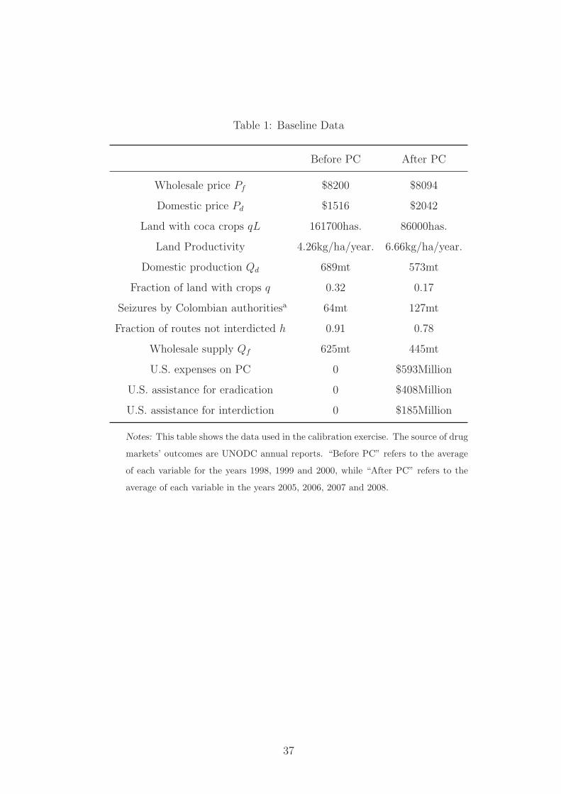
Table 1: Baseline Data

Before PC After PC

Wholesale price Pf $8200 $8094

Domestic price Pd $1516 $2042

Land with coca crops qL 161700has. 86000has.

Land Productivity 4.26kg/ha/year. 6.66kg/ha/year.

Domestic production Qd 689mt 573mt

Fraction of land with crops q 0.32 0.17

Seizures by Colombian authoritiesa 64mt 127mt

Fraction of routes not interdicted h 0.91 0.78

Wholesale supply Qf 625mt 445mt

U.S. expenses on PC 0 $593Million

U.S. assistance for eradication 0 $408Million

U.S. assistance for interdiction 0 $185Million

Notes: This table shows the data used in the calibration exercise. The source of drug

markets’ outcomes are UNODC annual reports. “Before PC” refers to the average

of each variable for the years 1998, 1999 and 2000, while “After PC” refers to the

average of each variable in the years 2005, 2006, 2007 and 2008.

37

Table 2: Calibration Results: Structural Parameters and Estimated Subsidies.

Estimated Description

ω 0.43 Fraction of eradication paid by Colombia

[0.34-0.55]

Ω 0.36 Fraction of interdiction paid by Colombia

[0.24-0.51]

α 0.60 Participation of complementary factors in production

[0.43-0.79]

η 0.32 Participation of domestic drugs in trafficking

[0.27-0.40]

c1 0.32 Net cost per dollar received by producers

[0.21-0.53]

c2 0.13 Net cost per dollar received by traffickers

[0.07-0.27]

φ 0.39 Drug producers relative efficiency

[0.24-0.86]

γ 1.86 Drug traffickers relative efficiency

[1.02-3.67]

Notes: This table shows the baseline calibration results. Below each baseline

estimate, a 90% confidence interval is shown. This interval was estimated using

10.000 Montecarlo simulations.

38

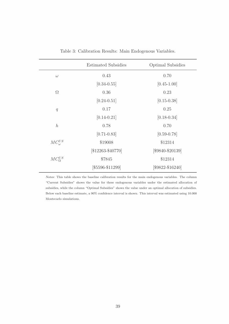
Table 3: Calibration Results: Main Endogenous Variables.

Estimated Subsidies Optimal Subsidies

ω 0.43 0.70

[0.34-0.55] [0.45-1.00]

Ω 0.36 0.23

[0.24-0.51] [0.15-0.38]

q 0.17 0.25

[0.14-0.21] [0.18-0.34]

h 0.78 0.70

[0.71-0.83] [0.59-0.78]

MCUSω $19008 $12314

[$12263-$40770] [$9840-$20139]

MCUSΩ $7845 $12314

[$5596-$11299] [$9822-$16240]

Notes: This table shows the baseline calibration results for the main endogenous variables. The column

“Current Subsidies” shows the value for these endogenous variables under the estimated allocation of

subsidies, while the column “Optimal Subsidies” shows the value under an optimal allocation of subsidies.

Below each baseline estimate, a 90% confidence interval is shown. This interval was estimated using 10.000

Montecarlo simulations.

39

Figure 1: The Distribution of Marginal Costs to the U.S.

MCUSΩ (actual)

$5596 $7845 $112990

1

2

×10−4

MCUSω (actual)

$12263 $19008 $407700

1

2

3

4

5

6

7

×10−5

Figure 2: Efficiency and budget gains

Efficiency gain

0.24% 2.43% 7.42%0

0.05

0.1

0.15

0.2

0.25

(A)

Budget gain

8.76% 12.83% 18.30%0

0.02

0.04

0.06

0.08

0.1

0.12

0.14

0.16

(B)

40

Figure 3: Simulation of a Budget Increase from MU.S = 0 to MU.S. = 1.5b.

Interested outsider expenditures Mo

Optimal subsidies ω (black) and Ω (blue)

0M 250M 500M 750M 1.000M 1.250M 1.500M0.1

0.2

0.3

0.4

0.5

0.6

0.7

0.8

0.9

1

Interested outsider expenditures Mo

q (black) and h (blue)

0M 250M 500M 750M 1.000M 1.250M 1.500M

0.2

0.3

0.4

0.5

0.6

0.7

0.8

0.9

Interested outsider expenditures Mo

MCU.S.ω (black) and MCU.S.

Ω (blue)

0M 250M 500M 750M 1.000M 1.250M 1.500M

0.5

1

1.5

2

2.5

×104

replacements

Interested outsider expenditures Mo

Conflict intensity (CI)

0M 250M 500M 750M 1.000M 1.250M 1.500M

1

1.5

2

2.5

3

3.5

×109

Interested outsider expenditures Mo

Wholesale supply Qf

0M 250M 500M 750M 1.000M 1.250M 1.500M

3

3.5

4

4.5

5

5.5

6

×105

Interested outsider expenditures Mo

Domestic production Qd

0M 250M 500M 750M 1.000M 1.250M 1.500M

5

5.5

6

6.5

7

7.5

8

×105

Interested outsider expenditures Mo

Wholesale price Pf

0M 250M 500M 750M 1.000M 1.250M 1.500M

6000

7000

8000

9000

10000

11000

12000

Interested outsider expenditures Mo

Domestic price Pd

0M 250M 500M 750M 1.000M 1.250M 1.500M

1400

1600

1800

2000

2200

2400

2600

41

6 Appendix A: Solving the model (not for publication)

6.1 The drug trafficking equilibrium:

We solve the game by backward induction. When choosing the demand for drugs in the

producer country, the drug trafficker’s problem is:

maxQd

πT = PfQf − PdQd − t, (A1)

taking Pf , Pd, t, s and h as given. The optimal choice of Qd is given by the following first

order condition:

∂πT∂Qd

= 0 ⇐⇒ Q∗

d = κh

(ηPfPd

) 11−η

(A2)

When choosing t, the trafficker anticipates his choice of Qd; therefore, the optimal choice

must solve the following problem:

maxt

π∗

T = ρhκP

11−η

f

Pη

1−η

d

− t, (A3)

where ρ = ηη

1−η − η1

1−η > 0. π∗

T is obtained by plugging Q∗

d into the original drug

trafficker’s problem. Using the expression for h from equation 3, the optimal choice of t is

given by the following first order condition:

∂π∗

T

∂t= 0 ⇐⇒ t∗ =

√√√√√ρκP

11−η

f s

γPη

1−η

d

−s

γ. (A4)

Equation A4 describes the drug trafficker’s reaction function in the conflict against the

government over the control of drug routes.

When choosing s, the government anticipates the subsequent trafficker’s choice of Qd;

therefore, its optimal choice must solve the following problem:

mins

CT = ηη

1−η c2hκP

11−η

f

Pη

1−η

d

+ Ωs, (A5)

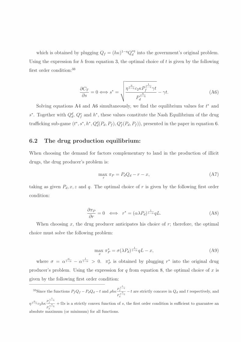
which is obtained by plugging Qf = (hκ)1−ηQ∗ηd into the government’s original problem.

Using the expression for h from equation 3, the optimal choice of t is given by the following

first order condition:33

∂CT∂s

= 0 ⇐⇒ s∗ =

√√√√√η

η1−η c2κP

11−η

f γt

Pη

1−η

d

− γt. (A6)

Solving equations A4 and A6 simultaneously, we find the equilibrium values for t∗ and

s∗. Together with Qdd, Q

sf and h∗, these values constitute the Nash Equilibrium of the drug

trafficking sub-game (t∗, s∗, h∗, Qdd(Pd, Pf ), Q

sf (Pd, Pf )), presented in the paper in equation 6.

6.2 The drug production equilibrium:

When choosing the demand for factors complementary to land in the production of illicit

drugs, the drug producer’s problem is:

maxrπP = PdQd − r − x, (A7)

taking as given Pd, x, z and q. The optimal choice of r is given by the following first order

condition:

∂πP∂r

= 0 ⇐⇒ r∗ = (αλPd)1

1−α qL. (A8)

When choosing x, the drug producer anticipates his choice of r; therefore, the optimal

choice must solve the following problem:

maxx

π∗

P = σ(λPd)1

1−α qL− x, (A9)

where σ = αα

1−α − α1

1−α > 0. π∗

P is obtained by plugging r∗ into the original drug

producer’s problem. Using the expression for q from equation 8, the optimal choice of x is

given by the following first order condition:

33Since the functions PfQf −PdQd− t and ρhκP

1

1−η

f

P

η1−η

d

− t are strictly concave in Qd and t respectively, and

ηη

1−η c2hκP

1

1−η

f

P

η1−η

d

+ Ωs is a strictly convex function of s, the first order condition is sufficient to guarantee an

absolute maximum (or minimum) for all functions.

∂π∗

P

∂x= 0 ⇐⇒ x∗ =

√

σ(λPd)1

1−αLz

φ−z

φ. (A10)

When choosing z, the government anticipates the drug producer’s subsequent choice of

r; therefore, its optimal choice must solve the following problem:

minz

CP = c1αα

1−αλα

1−αP1

1−α

d qL+ ωz, (A11)

which is obtained by plugging Qd = αα

1−α (λPd)α

1−α qL into the government’s original

problem. Using the expression for q from equation 8, the optimal choice of z is given by the

following first order condition 34

∂CP∂z

= 0 ⇐⇒ z∗i =

√

c1αα

1−α (λPd)1

1−αLφx

ω− φx. (A12)

Solving equations A10 and A12 simultaneously for x and z we find their equilibrium

values. Together with equation A8 and the implied value for q, these values constitute the

Nash Equilibrium of the drug production sub-game (x∗, z∗, q∗, r∗, Qsd(Pd)), presented in the

paper in equations 11.

6.3 The drug market equilibrium:

The domestic drug market equilibrium condition is given by:

q∗αα

1−αλ1

1−αPα

1−α

d L = h∗κ

(ηPfPd

) 11−η

, (A16)

while the international drug market equilibrium condition is given by:

h∗κ

(ηPfPd

) η1−η

=a

P bf

. (A17)

These equations form a simultaneous system of equations for Pd and Pf which turns out

to be log linear. Taking logs in both equations and using Cramer’s rule, we obtain:

34Since the functions PdQd − r − x, and σ(λPd)1

1−α qL − x are strictly concave in r and x respectively,

and the function c1αα

1−αλα

1−αP1

1−α

d qL + ωz is strictly convex in z, the first order conditions guarantee the

existence of a global maximum or minimum for all of these functions.

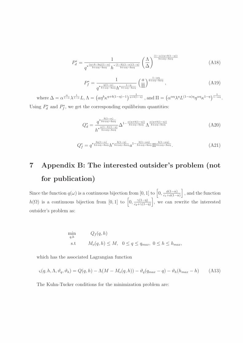
P ∗

d =1

q∗(η+b−bη)(1−α)

b+αη−bαη h∗(1−b)(1−α)(1−η)

b+αη−bαη

(Λ

∆

) (1−α)(η+b(1−η))b+αη−bαη

(A18)

P ∗

f =1

q∗η(1−α)

b+αη−bαηh∗1−η

b+αη−bαη

( a

Π

) 1−αηb+αη−bαη

, (A19)

where ∆ = αα

1−αλ1

1−αL, Λ =(aηbκη+b(1−η)−1

) 1η+b(1−η) , and Π =

(ααηληL(1−α)ηηαηκ1−η

) 11−αη .

Using P ∗

d and P ∗

f , we get the corresponding equilibrium quantities:

Q∗

d =q∗

b(1−α)b+αη−bαη

h∗α(1−b)(1−η)b+αη−bαη

∆1−α(η+b(1−η))b+αη−bαη Λ

α(η+b(1−η))b+αη−bαη (A20)

Q∗

f = q∗bη(1−α)

b+αη−bαηh∗b(1−η)

b+αη−bαη a1−b(1−αη)

b+αη−bαηΠb(1−αη)

b+αη−bαη . (A21)

7 Appendix B: The interested outsider’s problem (not

for publication)

Since the function q(ω) is a continuous bijection from [0, 1] to[

0, φ(1−α)c1+φ(1−α)

]

, and the function

h(Ω) is a continuous bijection from [0, 1] to[

0, γ(1−η)c2+γ(1−η)

]

, we can rewrite the interested

outsider’s problem as:

minq,h

Qf (q, h)

s.t Mo(q, h) ≤M, 0 ≤ q ≤ qmax, 0 ≤ h ≤ hmax,

which has the associated Lagrangian function

ς(q, h,Λ, ϑq, ϑh) = Q(q, h)− Λ(M −Mo(q, h))− ϑq(qmax − q)− ϑh(hmax − h) (A13)

The Kuhn-Tucker conditions for the minimization problem are:

q ≥ 0 , q

(∂Qf

∂q+ Λ

∂M

∂q+ ϑq

)

= 0,

h ≥ 0 , h

(∂Qf

∂h+ Λ

∂M

∂h+ ϑh

)

= 0,

Λ ≥ 0 , Λ(M −Mo(q, h)) = 0,

ϑq ≥ 0 , ϑq(qmax − q) = 0,

ϑh ≥ 0 , ϑh(hmax − h) = 0.

In any internal solution, we must have ϑq = ϑh = 0, and∂Qf

∂q+ Λ∂M

∂q=

∂Qf

∂h+ Λ∂M

∂h= 0,

which implies that:

MCω = −

∂M∂q

∂Qf

∂q

=1

Λ= −

∂M∂h∂Qf

∂h

=MCΩ (A14)

where MCω and MCΩ are the marginal cost of reducing the supply of drugs in interna-

tional drug markets by one kilogram by subsidizing the conflict over the control of arable

land (e.g. eradication efforts) and interdiction efforts, respectively. In this case, Λ > 0, and

we must also have M =Mo(q, h).

In a corner solution where q = qmax (or ω = 1), we must have ϑh = 0, and∂Qf

∂q+Λ∂M

∂q+

ϑq =∂Qf

∂h+ Λ∂M

∂h, which implies

MCω = −

∂M∂q

∂Qf

∂q

≥1

Λ= −

∂M∂h∂Qf

∂h

=MCΩ. (A15)

In this case, it is also true that Λ > 0, and we must also have M =M(q,h).

From the model we obtain:

Mo = A(1− q)

(Υ(1− q)

q− 1

)

q−Γh−ψ + B(1− h)

(Θ(1− h)

h− 1

)

q−Γy−ψ, (A16)

where Γ, ψ, Υ,Θ, A and B are themselves functions of the parameters of the model,

given by:

Γ =(1− α)(η − bη)

b+ αη − bαη, ψ =

(1− b)(1− η)

b+ αη − bαη,Υ =

φ(1− α)

c1,Θ =

γ(1− η)

c2,

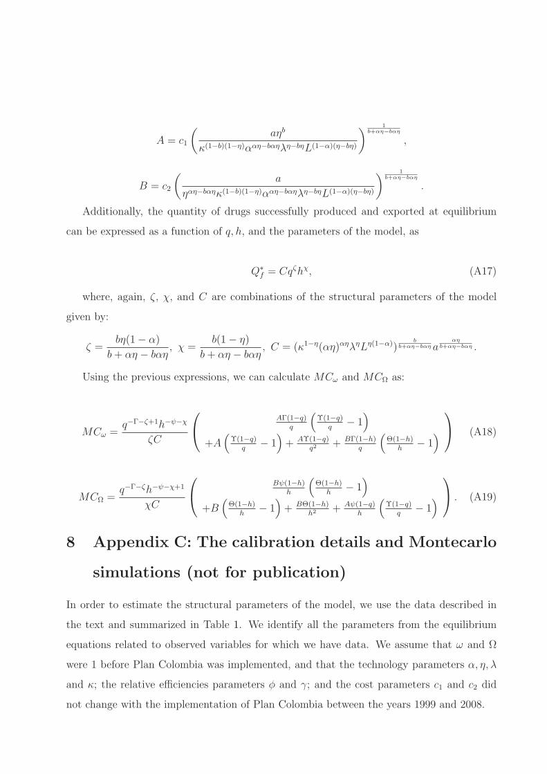
A = c1

(aηb

κ(1−b)(1−η)ααη−bαηλη−bηL(1−α)(η−bη)

) 1b+αη−bαη

,

B = c2

(a

ηαη−bαηκ(1−b)(1−η)ααη−bαηλη−bηL(1−α)(η−bη)

) 1b+αη−bαη

.

Additionally, the quantity of drugs successfully produced and exported at equilibrium

can be expressed as a function of q, h, and the parameters of the model, as

Q∗

f = Cqζhχ, (A17)

where, again, ζ, χ, and C are combinations of the structural parameters of the model

given by:

ζ =bη(1− α)

b+ αη − bαη, χ =

b(1− η)

b+ αη − bαη, C = (κ1−η(αη)αηληLη(1−α))

bb+αη−bαη a

αηb+αη−bαη .

Using the previous expressions, we can calculate MCω and MCΩ as:

MCω =q−Γ−ζ+1h−ψ−χ

ζC

AΓ(1−q)q

(Υ(1−q)

q− 1

)

+A(

Υ(1−q)q

− 1)

+ AΥ(1−q)q2

+ BΓ(1−h)q

(Θ(1−h)

h− 1

)

(A18)

MCΩ =q−Γ−ζh−ψ−χ+1

χC

Bψ(1−h)h

(Θ(1−h)

h− 1

)

+B(

Θ(1−h)h

− 1)

+ BΘ(1−h)h2

+ Aψ(1−q)h

(Υ(1−q)

q− 1

)

. (A19)

8 Appendix C: The calibration details and Montecarlo

simulations (not for publication)

In order to estimate the structural parameters of the model, we use the data described in

the text and summarized in Table 1. We identify all the parameters from the equilibrium

equations related to observed variables for which we have data. We assume that ω and Ω

were 1 before Plan Colombia was implemented, and that the technology parameters α, η, λ

and κ; the relative efficiencies parameters φ and γ; and the cost parameters c1 and c2 did

not change with the implementation of Plan Colombia between the years 1999 and 2008.

The U.S. expenditure figures are obtained from the GAO (2008) report. To approximate

the assistance at each front, we studied the description of each program and postulated an

hypothetical division of resources between both fronts in the following way: we treated 100%

of the resources allocated to the program as being used for one particular front when it is

very clear that it contributes mostly to this specific front and makes little or no contribution

to the other; we treat 80% of the resources allocated to the program as being used for one

particular front when its description relates the main function or objective of this program

to this front, yet recognize that some of its components are used for the other front; finally,

we treat 50% of the resources allocated to the program as being used for both fronts if its

aim is to improve the results in both fronts without explicitly being related to one or the

other.35 Table A1 shows the GAO (2008) data and our hypothetical division of resources

between the eradication and interdiction fronts for each program.36

8.1 The functional form parameters

For the demand parameters, we already have an imposed value, b = 0.65. We use the demand

functional form to estimate the scale parameter a. Once we fix b, we get

a = QfPbf .⇒ a ≃ 154, 447. (A20)

This parameter’s only role is to scale the market demand in order to obtain prices and

quantities in the correct order of magnitude.

For the trafficking front, we have that η is the share of domestic cocaine in the trafficking

35There are some programs reported as Other or Not allocated. We assume that they contribute the same

share to both fronts as other resources allocated for programs in cooperation with the same agency that

receives them (police or army).36We calculate the annual average by dividing totals by the number of years during which they were used-

that is 8 years- since the first Plan Colombia airborne mission flew at the end of 2000. In fact, our data

source, the GAO, recognizes that these expenditure figures correspond to the time during which they were

provided; this does not imply that they were actually spend at that time. For example, during the fiscal

year 2000, $818 million was provided to Plan Colombia, but the Plan itself only began at the end of that

year.

technology. Since we are using a Cobb Douglas function, we use the well known result

η =PdQd

PfQf

⇒ η ≃ 0.32. (A21)

The point estimate for η would be the same for any trafficking technology, but our assumed

Cobb Douglas technology allows us to use this value as fixed in our simulations. The above

formula requires price taker traffickers; otherwise, the final price might include a mark-up

and we would underestimate η. This estimate tells us that the trafficking technology is

“routes-intensive,” (e.g. 1 − η = 68%), while domestic cocaine relative importance is only

η = 32%.

The scale parameter is recovered from the trafficking technology functional form in order

to adjust the order of magnitude of quantities in this market. More precisely,

κ =1

h

(Qf

Qηd

) 11−η

⇒ κ ≃ 507, 336. (A22)

On the production front, we use the expression for land productivity in order to estimate

α. From the model, it follows that the productivity per hectare (prod) is given by:

prodB = αα

1−αλ1

1−αPα

1−α

dB and prod = αα

1−αλ1

1−αPα

1−α

d . (A23)

Log linearizing this equations and isolating α we obtain

α =ln(prodBprod

)

ln(PdB

Pd

)

+ ln(prodBprod

) ⇒ α ≃ 0.60. (A24)

The parameter α is identified from the log linear relation between land productivity and

domestic prices predicted by the model. In fact, the model tells us that

log(prod) = log(

αα

1−αλ1

1−α

)

+α

1− αlogPd (A25)

Hence, there is a positive linear relation between the percent change in land productivity and

domestic prices- implying that a 1% increase in prices corresponds to a α1−α

% increase in land

productivity. A larger value of α reflects a larger response of land productivity to domestic

prices, since producers can invest heavily on complementary factors when the domestic price

increases in order to counteract the effects of eradication campaigns. Our “big” value for

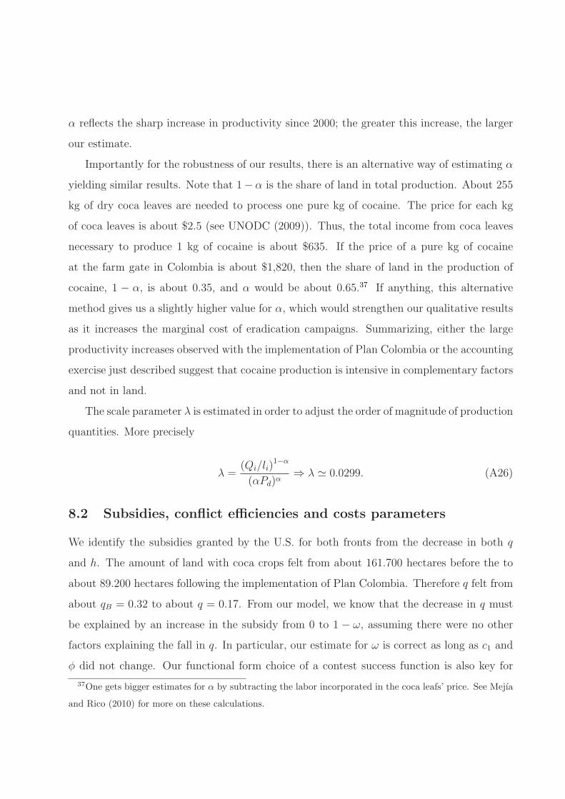
α reflects the sharp increase in productivity since 2000; the greater this increase, the larger

our estimate.

Importantly for the robustness of our results, there is an alternative way of estimating α

yielding similar results. Note that 1− α is the share of land in total production. About 255

kg of dry coca leaves are needed to process one pure kg of cocaine. The price for each kg

of coca leaves is about $2.5 (see UNODC (2009)). Thus, the total income from coca leaves

necessary to produce 1 kg of cocaine is about $635. If the price of a pure kg of cocaine

at the farm gate in Colombia is about $1,820, then the share of land in the production of

cocaine, 1 − α, is about 0.35, and α would be about 0.65.37 If anything, this alternative

method gives us a slightly higher value for α, which would strengthen our qualitative results

as it increases the marginal cost of eradication campaigns. Summarizing, either the large

productivity increases observed with the implementation of Plan Colombia or the accounting

exercise just described suggest that cocaine production is intensive in complementary factors

and not in land.

The scale parameter λ is estimated in order to adjust the order of magnitude of production

quantities. More precisely

λ =(Qi/li)

1−α

(αPd)α⇒ λ ≃ 0.0299. (A26)

8.2 Subsidies, conflict efficiencies and costs parameters

We identify the subsidies granted by the U.S. for both fronts from the decrease in both q

and h. The amount of land with coca crops felt from about 161.700 hectares before the to

about 89.200 hectares following the implementation of Plan Colombia. Therefore q felt from

about qB = 0.32 to about q = 0.17. From our model, we know that the decrease in q must

be explained by an increase in the subsidy from 0 to 1 − ω, assuming there were no other

factors explaining the fall in q. In particular, our estimate for ω is correct as long as c1 and

φ did not change. Our functional form choice of a contest success function is also key for

37One gets bigger estimates for α by subtracting the labor incorporated in the coca leafs’ price. See Mejıa

and Rico (2010) for more on these calculations.

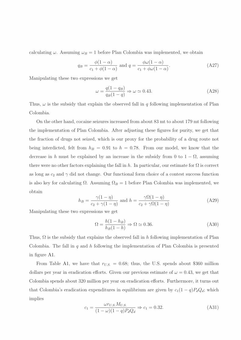
calculating ω. Assuming ωB = 1 before Plan Colombia was implemented, we obtain

qB =φ(1− α)

c1 + φ(1− α)and q =

φω(1− α)

c1 + φω(1− α). (A27)

Manipulating these two expressions we get

ω =q(1− qB)

qB(1− q)⇒ ω ≃ 0.43. (A28)

Thus, ω is the subsidy that explain the observed fall in q following implementation of Plan

Colombia.

On the other hand, cocaine seizures increased from about 83 mt to about 179 mt following

the implementation of Plan Colombia. After adjusting these figures for purity, we get that

the fraction of drugs not seized, which is our proxy for the probability of a drug route not

being interdicted, felt from hB = 0.91 to h = 0.78. From our model, we know that the

decrease in h must be explained by an increase in the subsidy from 0 to 1 − Ω, assuming

there were no other factors explaining the fall in h. In particular, our estimate for Ω is correct

as long as c2 and γ did not change. Our functional form choice of a contest success function

is also key for calculating Ω. Assuming ΩB = 1 before Plan Colombia was implemented, we

obtain

hB =γ(1− η)

c2 + γ(1− η)and h =

γΩ(1− η)

c2 + γΩ(1− η)(A29)

Manipulating these two expressions we get

Ω =h(1− hB)

hB(1− h)⇒ Ω ≃ 0.36. (A30)

Thus, Ω is the subsidy that explains the observed fall in h following implementation of Plan

Colombia. The fall in q and h following the implementation of Plan Colombia is presented

in figure A1.

From Table A1, we have that rU.S. = 0.68; thus, the U.S. spends about $360 million

dollars per year in eradication efforts. Given our previous estimate of ω = 0.43, we get that

Colombia spends about 320 million per year on eradication efforts. Furthermore, it turns out

that Colombia’s eradication expenditures in equilibrium are given by c1(1 − q)PdQd; which

implies

c1 =ωrU.S.MU.S.

(1− ω)(1− q)PdQd

⇒ c1 = 0.32. (A31)

Thus, c1 is identified from the joint expenditures on the eradication front, which are propor-

tional to c1 in equilibrium.

Similarly, given our previous estimate of Ω = 0.36 and the fact that the U.S. spends

about $234 million per year in interdiction efforts, Colombia spends about $117 million in

this front of the war on drugs. It turns out that Colombia’s interdiction expenditures in

equilibrium are given by c2(1− h)PfQf ; which implies

c2 =Ω(1− rU.S.)MU.S.

(1− Ω)(1− h)PfQf

⇒ c2 = 0.13. (A32)

Thus, c2 is identified from the joint expenditures on the interdiction front, which are pro-

portional to c2 in equilibrium.

The estimation of c1 and c2 relies heavily on our assumed functional forms for the Colom-

bian government problem. Intuitively, our estimation of these costs reflects the fact that the

Colombian government allocates resources to each front depending, among other things, on

the costs it perceives are generated at each stage, by either producers or traffickers.

Finally, in order to estimate φ and γ we use the equilibrium expressions for q and h.

Isolating φ from the equilibrium equation for q, we get

φ =qc1

ω(1− α)(1− q)→ φ = 0.39. (A33)

Similarly, for γ we obtain

γ =hc2

Ω(1− η)(1− h)→ γ = 1.86. (A34)

8.3 Other endogenous variables of interest

We can also calculate other important variables of the model, both under an current alloca-

tion (“Current subsidies”), and the optimal allocation of subsidies (“Optimal subsidies”).

Table A2 shows the main endogenous variables related to the drug trafficking front.

According to our estimates, drug traffickers spend about $542 million per year in avoiding

the interdiction of drug routes, t. Additionally, traffickers spend $1.2 billion buying drugs

from domestic producers, leaving them with a profit of about $1.9 billion per year. These

figures imply an average rate of return from illegal drug trafficking activities, calculated as

the ratio of total profits to total costs, of roughly 111%. On the other hand, Colombia

and the U.S. have spent about $288 million on interdiction. Out of this, the Colombian

government has contributed about $103 million (Ωs) and the U.S. government about $185

million ((1 − Ω)s). Based on these estimates along with that for c2, we find that the costs

perceived by the government arising from cocaine trafficking, CT , are about $564 million per

year since implementation of Plan Colombia.

Table A3 shows the main endogenous variables related to the drug production front.

We estimate that drug producers spend about $387 million per year fighting the Colombian

government over the control of arable land, x. Furthermore, drug producers spend about $702

million per year on factors complementary to land in the production of cocaine (chemical

precursors, workshops, labor, etc.), leaving them with a profit of about $80 million per

year.38 These figures imply an average rate of return from illegal drug production activities,

calculated as the ratio of total profits to total costs, of roughly 7%. On the other hand,

Colombia and the U.S. spent about $722 million per year on eradication efforts. Out of this,

the Colombian government contributed $314 million (ωz) and the U.S. government about

$408 million ((1 − ω)z). Based on these estimates along that for c1, we find that that the

total costs perceived by the Colombian government arising from cocaine production, CP , are

about $692 million per year since the implementation of Plan Colombia.

8.4 Montecarlo simulations

In order to test the sensibility of our results with respect to the data used in the baseline

calibration, we conduct 10,000 Montecarlo simulations. For each simulation we draw a

random sample of the observations used to calibrate the model from a normal distribution

38According to a press release from the Office of National Drug Control Policy, FARC drug profits in 2005

ranged between $60 and $115 million (See http://www.whitehousedrugpolicy.gov/pda/060407.html). Our

estimate for FARC drug profits of $40 million for 2005-2008 (half of total profits, inasmuch as the other

half is in the hands of paramilitary groups), is not far from that obtained by other sources, especially if

one takes into account that FARC are also involved in the very initial stages of cocaine trafficking inside

Colombia. The same press release also mentions that FARC drug profits per kilogram of cocaine produced

range between $195 and $320. Our estimate for FARC drug profits per kilogram of cocaine successfully

produced is $140. Again, this figure does not include FARC profits from cocaine trafficking.

centered around their baseline value, with a standard deviation equal to 7.5% of these values,

and truncated at twice and half the baseline value of the observations. We do this for all

the variables required for the calibration, including seizures; the purity level used to adjust

them; the price elasticity of demand; U.S. expenditures; the potential land available for coca

cultivation; drug prices; productivities; and the amount of land with coca crops. Thus, for

example, for the productivity per hectare after Plan Colombia, we obtain a vector of 10,000

random draws from a normal distribution with mean 6.66 (its current value, used in the

baseline scenario), a standard deviation equal to 0.5, and truncated at 3.33 and 13.32. We

truncate the variables to avoid unrealistic observations, such as negative prices or quantities.

For each of the 10.000 observations samples, we calibrate all the parameters using the

equations described in the previous section. We obtain 10,000 samples of calibrated param-

eters. For each of these calibrated parameters’ sample, we also estimate all the relevant

endogenous variables. We end up with 10,000 estimations for each parameter or endogenous

variable, which allow us to construct their empirical distribution and 90% confidence inter-

vals. The figures showing the distributions for all structural parameters and the endogenous

variables of interest are available from the authors upon request.

Finally, for each of the 10,000 sets of calibrated parameters, we conduct simulations of

an exogenous U.S. budget increase under an optimal allocation of subsidies. We use these

simulations to construct confidence intervals for different endogenous variables trajectories,

as shown in section 3.4. We also conducted simulations assuming different trajectories of

subsidies; these are available upon request.

8.5 Robustness checks

The first concern with our calibration exercise has to do with its sensibility to the data used

in the baseline scenario. The Montecarlo simulations were precisely designed to address this

concern; they show that perturbing the data does not significantly change our qualitative

findings. In particular, our main results- namely that the U.S. would do better if it reallocated

resources from eradication to interdiction efforts, and that the marginal cost of reducing

wholesale drug supply by 1kg is of the order of $10,000 dollars- remain true under more than

90% of the simulations. This means that our results are not sensible to the data used and

are driven by the economic forces in our model.

A second concern relates to the assumptions made in the calibration exercise. The

fundamental assumption is that the structural parameters c1, c2, φ and γ did not change

with the implementation of Plan Colombia, and that the fall in q and h is entirely explained

by higher U.S. subsidies. It is conceivable that c1 and c2 could have changed during the

period 2000-2008. In addition to being subjective, c1 and c2 are determined by the nature of

Colombia civil conflict and the actors involved in it, both of which are constantly changing.

Moreover, the relative efficiency of traffickers and producers (φ and γ) could have changed

because of alliances, merges between or disruptions of the illegal groups associated with

these illicit activities. It could also be the case that spillovers from other forms of military

expenditures by the Colombia’s government affected these relative efficiencies.

If any of these parameters changed between 2000 and 2008, our estimates for the subsidies

would be biased. Most likely, we would be over-estimating the subsidies by assuming that

they are entirely responsible for improvements in eradication and interdiction efforts. In

order to address this potential concern, we directly impose values for the current subsidies

instead of estimating them. Figure A2.A, shows the effects of imposing different values for

ω, while figure A2.B shows the effects of imposing different values for Ω. We only report the

effect on the estimated marginal costs under the current and optimal allocation of subsidies,

which summarize most of the important information. These figures show a clear pattern:

the marginal cost by subsidizing a particular front of the war on drugs increases with the

assumed value for ω or Ω, while the marginal cost in the other front remains constant.

The intuition behind this result is that having a lower value than the real one for ω or Ω,

implies that we were overestimating the subsidies; hence, we were attributing to eradication

or interdiction efforts improvements that they did not achieve. For instance, if ω and Ω

turned out to be larger, as would be the case if there were other factors explaining the fall

in q and h, we would get even larger marginal costs. Our inefficiency result is very robust,

since interdiction remains more cost effective as long as the current value for Ω does not get

too close to 1.39

39The assumptions behind the estimation of η and α are discussed in the appendix. We do not construct

robustness checks for these since other authors obtain similar estimations for these parameters (See Mejıa

Another concern has to do with the values of the parameters we do not estimate or

observe, but rather directly assume in the calibration, such as the price elasticity of demand

and the share of U.S. assistance allocated to eradication and interdiction efforts.40 Although

we already included perturbations in these variables in the Montecarlo simulations, we also

conduct a sensibility analysis wherein we change the assumed value of these parameters while

leaving all other baseline data unchanged. Figure A2.C, shows the effects on the estimated

marginal costs of assuming a value between 20% and 80% for the share of U.S. assistance

allocated to eradication efforts. Recall that the value used in the base line scenario was

68.8%. Interdiction remains more cost effective as long as the share of resources allocated by

the U.S. to eradication efforts is larger than 47%, as can be seen in this figure. Moreover, the

marginal cost under an optimal allocation of subsidies is not very sensitive to these changes.

Figure A2.D shows the effects on the marginal costs of assuming a value for b between 0.2

and 1. Recall that the value used in the base line scenario was 0.65. As can be seen in

this figure, a higher price elasticity of demand (e.g. a more elastic demand) decreases the

costs and increases the effectiveness of anti-drug policies. As long as demand is inelastic,

our results do not change significantly. Moreover, the value of the price elasticity of demand

affects both fronts’ marginal costs in a similar way; therefore, interdiction remains a more

cost effective policy.

The last concern is about the sensibility of our results with respect to the assumed func-

tional forms, especially the Cobb-Douglas technologies. Although these functional forms are

required to conduct the simulations, one could introduce them as log linear approximations

of generic production and trafficking functions. Moreover, the point estimates for the elas-

ticities involved in these technologies, α and η, remains valid even in a more general case.

Furthermore, the analytical expressions for equilibrium quantities and expenditures can also

be seen as log linear approximations. Therefore, while assuming functional forms appears

restrictive, many of our results hold under more generally functional forms, at least locally.

The contest success functions are required in order to calibrate the model, but we do not

and Rico (2010)).40We also assume the seizures’ purity (70%), but modifying this value does not change our model or results

in any significant way.

think our results are very sensible to the generic form that is assumed as long as they are

homogeneous of degree zero.

9 Appendix D: The optimal allocation of subsidies from

the Colombian point of view (not for publication)

Let CP = c1PdQd + ωz be the total cost to Colombia from drug production activities;

CT = c2PfQf+Ωs the total cost to Colombia from drug trafficking activities; MT = (1−Ω)s

the U.S. allocation of resources for interdiction efforts; andMP = (1−ω)z the U.S. allocation

of resources for the conflict over the control of arable land. If Colombia were allowed to choose

the subsidies for each front of the war on drugs, it would choose them as to solve the following

optimization problem:

minω,Ω

CT + CP s.t. MT +MP ≤M,

0 ≤ ω,Ω ≤ 1.

In order to be consistent with our model, we assume that Colombia takes prices as given;

therefore, we take the equilibrium values for CT , CP ,MT and MP as functions of market

prices and the parameters of the model.

For any internal solution, the following condition must hold:

(

−∂C∗

T

∂M∗

T

)

Ω

=

(

−∂C∗

P

∂M∗

P

)

ω

. (A35)

This optimality condition states that each extra dollar of U.S. assistance used for eradication

decreases the total cost of conflict to Colombia (CT +CP ) by the same amount as one extra

dollar of U.S. assistance invested in interdiction efforts. This condition can fail to be true

only if we have a corner solution with either ω∗ = 1 or Ω∗ = 1.

By using the equilibrium values for all variables, but in this case taking prices as exoge-

nous, we get:

CT = h(2− h)c2κηη

1−ηPf

(PfPd

) η1−η

, (A36)

CP = q(2− q)c1λ1

1−αLαα

1−αP1

1−α

d , (A37)

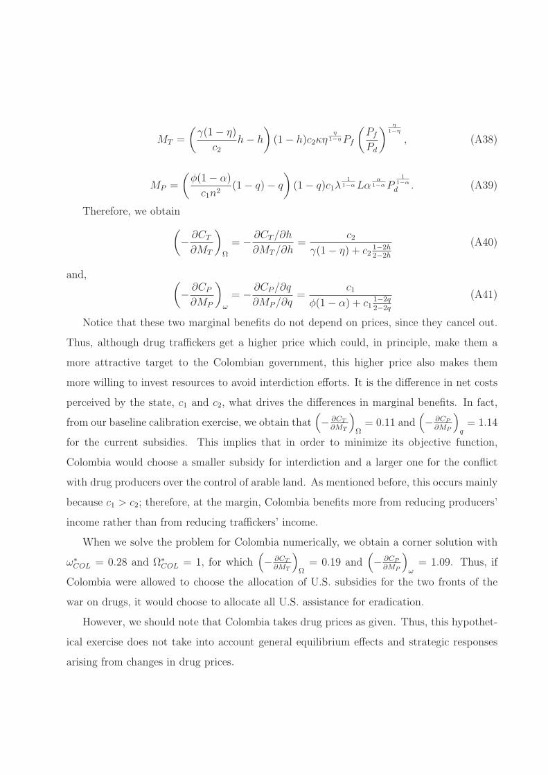
MT =

(γ(1− η)

c2h− h

)

(1− h)c2κηη

1−ηPf

(PfPd

) η1−η

, (A38)

MP =

(φ(1− α)

c1n2(1− q)− q

)

(1− q)c1λ1

1−αLαα

1−αP1

1−α

d . (A39)

Therefore, we obtain

(

−∂CT∂MT

)

Ω

= −∂CT/∂h

∂MT/∂h=

c2

γ(1− η) + c21−2h2−2h

(A40)

and,(

−∂CP∂MP

)

ω

= −∂CP/∂q

∂MP/∂q=

c1

φ(1− α) + c11−2q2−2q

(A41)

Notice that these two marginal benefits do not depend on prices, since they cancel out.

Thus, although drug traffickers get a higher price which could, in principle, make them a

more attractive target to the Colombian government, this higher price also makes them

more willing to invest resources to avoid interdiction efforts. It is the difference in net costs

perceived by the state, c1 and c2, what drives the differences in marginal benefits. In fact,

from our baseline calibration exercise, we obtain that(

− ∂CT

∂MT

)

Ω= 0.11 and

(

− ∂CP

∂MP

)

q= 1.14

for the current subsidies. This implies that in order to minimize its objective function,

Colombia would choose a smaller subsidy for interdiction and a larger one for the conflict

with drug producers over the control of arable land. As mentioned before, this occurs mainly

because c1 > c2; therefore, at the margin, Colombia benefits more from reducing producers’

income rather than from reducing traffickers’ income.

When we solve the problem for Colombia numerically, we obtain a corner solution with

ω∗

COL = 0.28 and Ω∗

COL = 1, for which(

− ∂CT

∂MT

)

Ω= 0.19 and

(

− ∂CP

∂MP

)

ω= 1.09. Thus, if

Colombia were allowed to choose the allocation of U.S. subsidies for the two fronts of the

war on drugs, it would choose to allocate all U.S. assistance for eradication.

However, we should note that Colombia takes drug prices as given. Thus, this hypothet-

ical exercise does not take into account general equilibrium effects and strategic responses

arising from changes in drug prices.

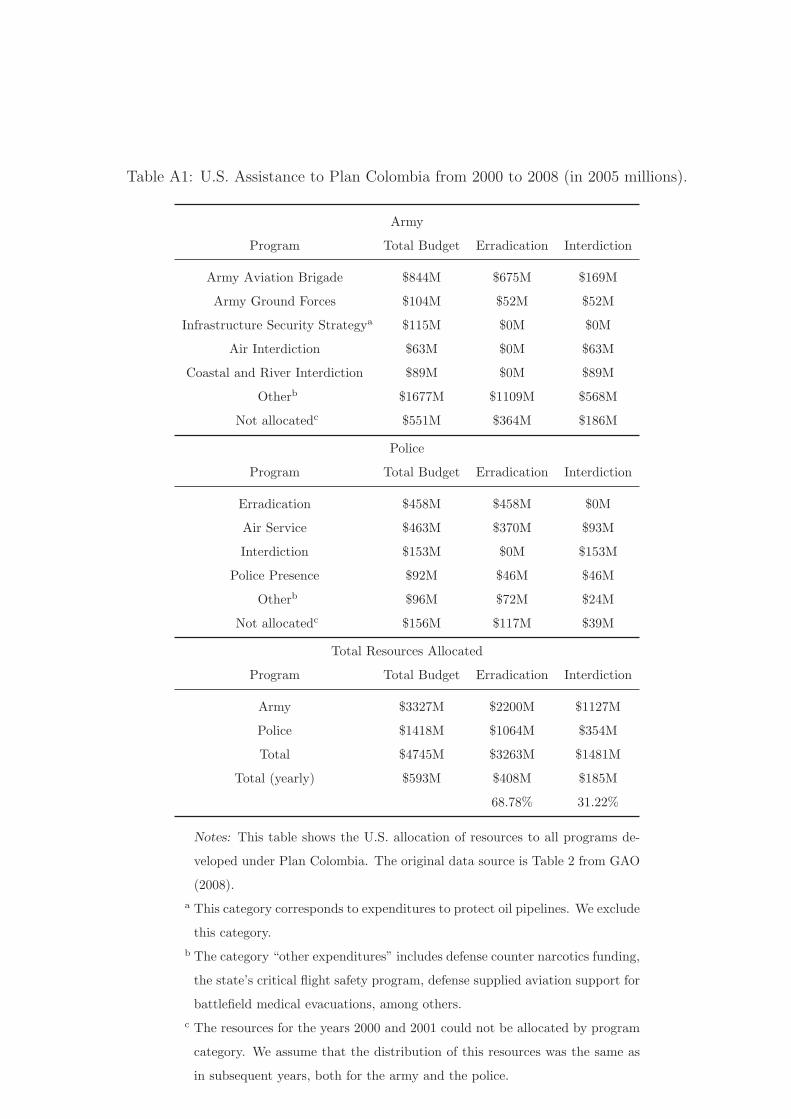
Table A1: U.S. Assistance to Plan Colombia from 2000 to 2008 (in 2005 millions).

Army

Program Total Budget Erradication Interdiction

Army Aviation Brigade $844M $675M $169M

Army Ground Forces $104M $52M $52M

Infrastructure Security Strategya $115M $0M $0M

Air Interdiction $63M $0M $63M

Coastal and River Interdiction $89M $0M $89M

Otherb $1677M $1109M $568M

Not allocatedc $551M $364M $186M

Police

Program Total Budget Erradication Interdiction

Erradication $458M $458M $0M

Air Service $463M $370M $93M

Interdiction $153M $0M $153M

Police Presence $92M $46M $46M

Otherb $96M $72M $24M

Not allocatedc $156M $117M $39M

Total Resources Allocated

Program Total Budget Erradication Interdiction

Army $3327M $2200M $1127M

Police $1418M $1064M $354M

Total $4745M $3263M $1481M

Total (yearly) $593M $408M $185M

68.78% 31.22%

Notes: This table shows the U.S. allocation of resources to all programs de-

veloped under Plan Colombia. The original data source is Table 2 from GAO

(2008).

a This category corresponds to expenditures to protect oil pipelines. We exclude

this category.

b The category “other expenditures” includes defense counter narcotics funding,

the state’s critical flight safety program, defense supplied aviation support for

battlefield medical evacuations, among others.

c The resources for the years 2000 and 2001 could not be allocated by program

category. We assume that the distribution of this resources was the same as

in subsequent years, both for the army and the police.

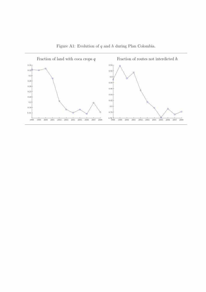
Figure A1: Evolution of q and h during Plan Colombia.

Fraction of land with coca crops q

1998 1999 2000 2001 2002 2003 2004 2005 2006 2007 2008

0.16

0.18

0.2

0.22

0.24

0.26

0.28

0.3

0.32

0.34

Fraction of routes not interdicted h

1998 1999 2000 2001 2002 2003 2004 2005 2006 2007 20080.76

0.78

0.8

0.82

0.84

0.86

0.88

0.9

0.92

0.94

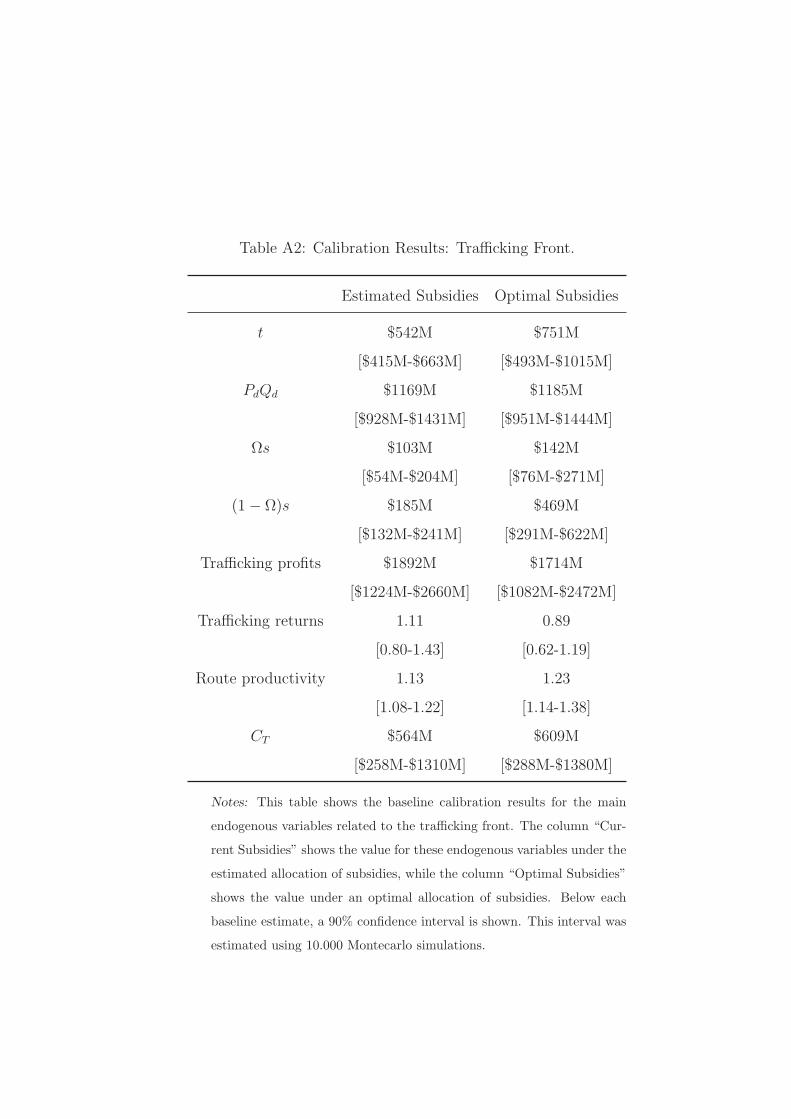
Table A2: Calibration Results: Trafficking Front.

Estimated Subsidies Optimal Subsidies

t $542M $751M

[$415M-$663M] [$493M-$1015M]

PdQd $1169M $1185M

[$928M-$1431M] [$951M-$1444M]

Ωs $103M $142M

[$54M-$204M] [$76M-$271M]

(1− Ω)s $185M $469M

[$132M-$241M] [$291M-$622M]

Trafficking profits $1892M $1714M

[$1224M-$2660M] [$1082M-$2472M]

Trafficking returns 1.11 0.89

[0.80-1.43] [0.62-1.19]

Route productivity 1.13 1.23

[1.08-1.22] [1.14-1.38]

CT $564M $609M

[$258M-$1310M] [$288M-$1380M]

Notes: This table shows the baseline calibration results for the main

endogenous variables related to the trafficking front. The column “Cur-

rent Subsidies” shows the value for these endogenous variables under the

estimated allocation of subsidies, while the column “Optimal Subsidies”

shows the value under an optimal allocation of subsidies. Below each

baseline estimate, a 90% confidence interval is shown. This interval was

estimated using 10.000 Montecarlo simulations.

Table A3: Calibration Results: Production Front.

Estimated Subsidies Optimal Subsidies

x $387M $355M

[$188M-$569M] [$158M-$549M]

r $702M $711M

[$467M-$951M] [$472M-$970M]

ωz $314M $288M

[$201M-$515M] [$184M-$477M]

(1− ω)z $408M $124M

[$339M-$481M] [$0M-$299M]

Production profits $80M $119M

[$38M-$128M] [$69M-$168M]

Production returns 0.07 0.11

[0.04-0.11] [0.07-0.16]

Land productivity 6.66 5.36

[5.82-7.47] [4.12-6.52]

CP $692M $671M

[$440M-$1145M] [$426M-$1114M]

Notes: This table shows the calibration results for the main endogenous

variables related to the production front. The column “Current Subsi-

dies” shows the value for these endogenous variables under the estimated

allocation of subsidies, while the column “Optimal Subsidies” shows the

value under an optimal allocation of subsidies. Below each baseline es-

timate, a 90% confidence interval is shown. This interval was estimated

using 10.000 Montecarlo simulations.

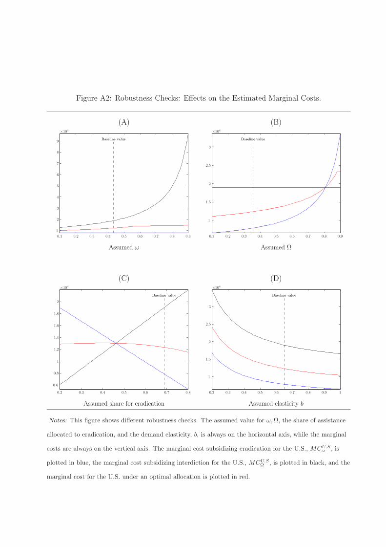
Figure A2: Robustness Checks: Effects on the Estimated Marginal Costs.

(A)

Baseline value

Assumed ω

0.1 0.2 0.3 0.4 0.5 0.6 0.7 0.8 0.9

1

2

3

4

5

6

7

8

9

×104

(B)

Baseline value

Assumed Ω

0.1 0.2 0.3 0.4 0.5 0.6 0.7 0.8 0.9

1

1.5

2

2.5

3

×104

(C)

Baseline value

Assumed share for eradication

0.2 0.3 0.4 0.5 0.6 0.7 0.8

0.6

0.8

1

1.2

1.4

1.6

1.8

2

×104

(D)

Baseline value

Assumed elasticity b

0.2 0.3 0.4 0.5 0.6 0.7 0.8 0.9 1

1

1.5

2

2.5

3

×104

Notes: This figure shows different robustness checks. The assumed value for ω,Ω, the share of assistance

allocated to eradication, and the demand elasticity, b, is always on the horizontal axis, while the marginal

costs are always on the vertical axis. The marginal cost subsidizing eradication for the U.S., MCU.Sω , is

plotted in blue, the marginal cost subsidizing interdiction for the U.S., MCU.SΩ , is plotted in black, and the

marginal cost for the U.S. under an optimal allocation is plotted in red.