The Voice of Optimization

Dimitris Bertsimas and Bartolomeo Stellato

June 3, 2020

Abstract

We introduce the idea that using optimal classification trees(OCTs) and optimal classification trees with-hyperplanes (OCT-Hs),interpretable machine learning algorithms developed by Bertsimasand Dunn [2017, 2019], we are able to obtain insight on the strategybehind the optimal solution in continuous and mixed-integer convexoptimization problem as a function of key parameters that affect theproblem. In this way, optimization is not a black box anymore. In-stead, we redefine optimization as a multiclass classification problemwhere the predictor gives insights on the logic behind the optimalsolution. In other words, OCTs and OCT-Hs give optimizationa voice. We show on several realistic examples that the accuracybehind our method is in the 90%-100% range, while even when thepredictions are not correct, the degree of suboptimality or infeasibilityis very low. We compare optimal strategy predictions of OCTs andOCT-Hs and feedforward neural networks (NNs) and conclude thatthe performance of OCT-Hs and NNs is comparable. OCTs aresomewhat weaker but often competitive. Therefore, our approachprovides a novel insightful understanding of optimal strategies tosolve a broad class of continuous and mixed-integer optimizationproblems.

1 Introduction

Optimization has a long and distinguished history that has had and continuesto have genuine impact in the world. In a typical optimization problem in

1

arX

iv:1

812.

0999

1v3

[m

ath.

OC

] 2

Jun

202

0

the real world, practitioners see optimization as a black-box tool where theyformulate the problem and they pass it to a solver to find an optimal solu-tion. Especially in high dimensional problems typically encountered in realworld applications, it is currently not possible to interpret or intuitively un-derstand the optimal solution. However, independent from the optimizationalgorithm used, practitioners would like to understand how problem parame-ters affect the optimal decisions in order to get intuition and interpretabilitybehind the optimal solution. Moreover, in almost all real world applicationsof optimization the main objective is not to solve just one problem but tosolve multiple similar instances that vary slightly from each other. In fact, inmost real-world applications we solve similar optimization problems multipletimes with varying data depending on problem-specific parameters.

Our goal in this paper is to propose a framework to predict the optimalsolution as parameters of the problem vary and do so in an interpretable way.A naive approach could be to learn directly the optimal solution from theproblem parameters. However, this method is computationally intractableand imprecise: intractable, because it would require a potentially high di-mensional predictor with hundreds of thousands of components dependingon the decision variable size; imprecise, because it would involve a regressiontask that would naturally carry a generalization error leading to subopti-mal or even infeasible solutions. Instead, our approach encodes the optimalsolution with a small amount of information that we denote as strategy. De-pending on the problem class, a strategy can have different meanings but italways corresponds to the complete information needed to efficiently recoverthe optimal solution.

In recent times, machine learning has also had significant impact to theworld. Optimization methods has been a major driver of its success [Hastieet al., 2009, Bertsimas and Dunn, 2019]. In this paper, we apply machinelearning to optimization with the objective to give a voice to optimization,that is to provide interpretability and intuition behind optimal solutions.

First, we solve an optimization problem for many parameter combina-tions and obtain the optimal strategy: the set of active constraints as wellas the value of the discrete variables. Second, we encode the strategies withunique integer scalars. In this way, we have a mapping from parametersto the optimal solution strategies, which gives rise to a multiclass classifi-cation problem [Hastie et al., 2009]. We solve the multiclass classificationproblem using optimal classification trees (OCTs) and optimal classificationtrees with-hyperplanes (OCT-Hs) developed by Bertsimas and Dunn [2017,

2

2019], interpretable state of the art classification algorithms as well as neu-ral networks (NNs), which, while not interpretable, serve as a benchmark tocompare the accuracy of OCTs and OCT-Hs.

1.1 Related Work

There has been a significant interest from both the computer science and theoptimization communities to systematically analyze and solve optimizationproblems using machine learning. From the first works applying machinelearning as a substitute for mathematical optimization algorithms in the1990s [Smith, 1999], this research direction has been increasingly active untilrecent results on learning for combinatorial optimization [Bengio et al., 2018].

Learning to tune algorithms. Most optimization methods consist of it-erative routines with several parameters obtained through experts’ knowl-edge and manual tuning. For example, Gurobi optimizer has 157 param-eters [Gurobi Optimization, Inc., 2020] that are carefully tuned in everyrelease. However, this tuning can be, on the one hand, very complex becauseit concerns several aspects of the problem that are not known a priori and,on the other hand, suboptimal for the instances considered in a specific ap-plication. To overcome these limitations, the machine learning communitystudied the algorithm configuration problem, i.e., the problem of automati-cally tuning algorithms from the problem instances of interest. One of thefirst efficient automatic configuration methods is ParamILS [Hutter et al.,2009] which iteratively improves the algorithm parameters using local searchmethods. Hutter et al. [2011] extended this idea in SMAC, a frameworkto learn the relationship between algorithm configurations and performance.The proposed scheme relies on Gaussian Processes and Random Forests toperform the predictions. Later, Lopez-Ibanez et al. [2016] introduced irace,an algorithm that iteratively refines the candidate parameters configurationsto identify the best ones for a specific application. Despite their relevancein practice, these approaches aim to identify or predict the best algorithmparameters, independently from the algorithm ultimate task, i.e., they donot only consider optimization algorithms. In addition, they do not considerinterpretability of the predictors. For instance, SMAC could benefit frominterpretable predictors such as OCTs to allow the user to understand whysome parameter configurations are better than others. Our work, instead,

3

studies the relationship between the problem instances and the optimal solu-tion focusing specifically on optimization algorithms and the interpretabilityof the optimal solutions.

Learning heuristics. Optimization methods not only rely on careful param-eter tuning, but also on efficient heuristics. For example, branch-and-bound(B&B) involves several heuristic decisions about the branching behavior thatare hand-tuned into the solvers. However, heuristics tuning can be very com-plex because it concerns several aspects of the problem that are not knowna priori. Khalil et al. [2016] propose to learn the branching rules showingperformance improvements over commercial hand-tuned algorithms. Simi-larly, Alvarez et al. [2017] approximate strong branching rules with learningmethods. Machine learning has been useful also to select reformulations anddecompositions for mixed-integer optimization (MIO). Bonami et al. [2018]learn in which cases it is more efficient to solve mixed-integer quadratic op-timization problem (MIQO) by linearizing or not the cost function. Theymodel it as a classification problem showing advantages compared to howthis choice is made heuristically inside state-of-the-art solvers. Kruber et al.[2017] propose a similar method applied to decomposition selection for MIO.

Reinforcement learning for optimization. Another interesting line of re-search models optimization problems as control tasks to tackle using re-inforcement learning [Sutton and Barto, 2018]. Problems suitable to thisframework include knapsack-like or network problems with multistage de-cisions. Dai et al. [2017] develop a method to learn heuristics over graphproblems. In this way the node selection criterion becomes the output ofa specialized neural network that does not depend on the graph size [Daiet al., 2016]. Every time a new node is visited, Dai et al. [2017] feed a graphrepresentation of the problem to the NN obtaining a criterion suggesting thenext node to select in the optimal solution.

Learning constraint programs. Constraint programming is a paradigm tomodel and solve combinatorial optimization problems very popular in thecomputer science community. The first works on applying machine learn-ing to automatically configure constraint programs (CPs) date back to the1990s [Minton, 1996]. Later, Clarke et al. [2002] used Decision Trees toreplace computationally hard parts of counterexample guided SAT solving

4

algorithms. More recently, Xu et al. [2008] describe SATzilla, an automatedapproach for learning which candidate solvers are best on a given instance.SATzilla won several SAT solver competitions because if its ability to adaptand pick the best algorithm for a problem instance. Given a SAT instance,instead of solving it with different algorithms, SATzilla relies on a empiricalhardness model to predict how long each algorithm should take. This modelconsists of a ridge regressor [Hastie et al., 2009] after nonlinear transforma-tion of the problem features. Selsam et al. [2019] applied recent advances inNN archtectures to CPs by directly predicting the solution or infeasibility.Even though this approach did not give as good results as state-of-the-artmethods, it introduces a new research direction for solving CPs. Therefore,the constraint programming community is also working on data-driven meth-ods to improve the performance and understanding of solution algorithms.

Learning parametric programs. Even though recent approaches for inte-grating machine learning and optimization show promising results, they donot consider the parametric nature of the problems appearing in real-worldapplications. It is often the case that practitioners solve the same problemwith slightly varying parameters multiple times generating a large amountof data describing how the parameters affect the optimal solution. There areonly a few recent papers exploiting this information to build better solutionalgorithms. The idea of learning the set of active constraints for parametriconline optimization has been proposed by Misra et al. [2019]. The authorsframe the learning procedure as a sampling scheme where they collect allthe active sets appearing from the parameters. However, we found severallimitations of their approach. First, in the online phase, they evaluate allthe relevant active sets in parallel and pick the best one [Misra et al., 2019,ensemble policy ]. Therefore, they do not solve the optimization problem asa multiclass classification problem and they are not able to gain insightson how the parameters affect the optimal strategy. In addition, they donot tackle mixed-integer optimization problems but only continuous convexones. Finally, the sampling strategy by Misra et al. [2019] has to be tuned foreach specific problem since it depends on at least four different parameters.This is because the authors compute the probabilistic guarantees based onhow many new active sets appear over the samples in a window of a spe-cific size [Misra et al., 2019, Section 3]. In this work, instead, we providea concise Good-Turing estimator [Good, 1953] for the probability of find-

5

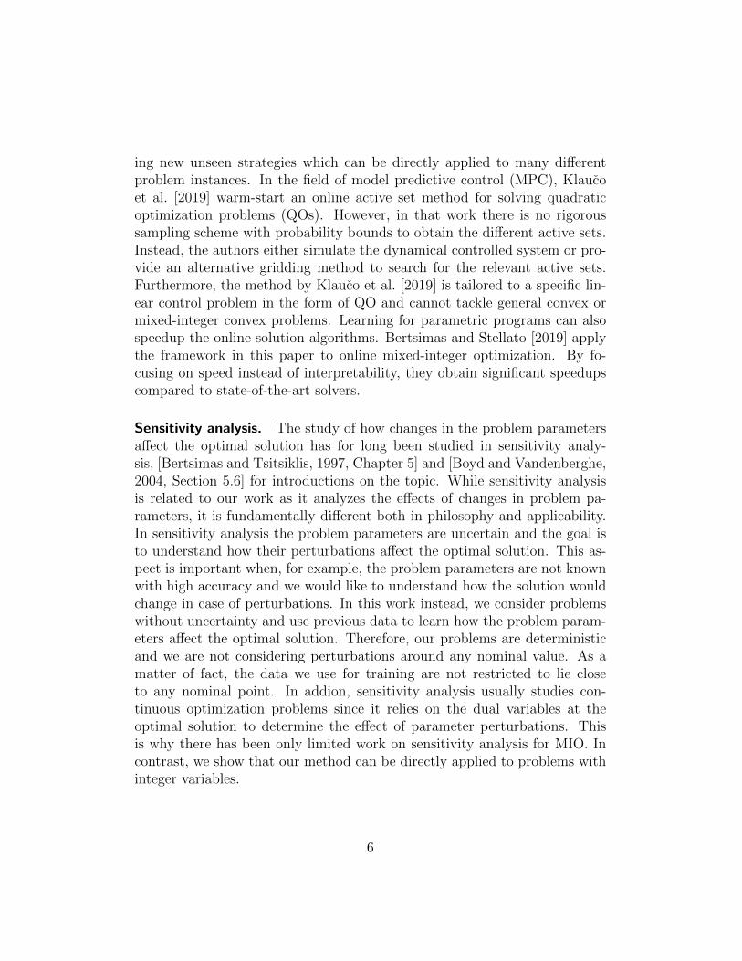
ing new unseen strategies which can be directly applied to many differentproblem instances. In the field of model predictive control (MPC), Klaucoet al. [2019] warm-start an online active set method for solving quadraticoptimization problems (QOs). However, in that work there is no rigoroussampling scheme with probability bounds to obtain the different active sets.Instead, the authors either simulate the dynamical controlled system or pro-vide an alternative gridding method to search for the relevant active sets.Furthermore, the method by Klauco et al. [2019] is tailored to a specific lin-ear control problem in the form of QO and cannot tackle general convex ormixed-integer convex problems. Learning for parametric programs can alsospeedup the online solution algorithms. Bertsimas and Stellato [2019] applythe framework in this paper to online mixed-integer optimization. By fo-cusing on speed instead of interpretability, they obtain significant speedupscompared to state-of-the-art solvers.

Sensitivity analysis. The study of how changes in the problem parametersaffect the optimal solution has for long been studied in sensitivity analy-sis, [Bertsimas and Tsitsiklis, 1997, Chapter 5] and [Boyd and Vandenberghe,2004, Section 5.6] for introductions on the topic. While sensitivity analysisis related to our work as it analyzes the effects of changes in problem pa-rameters, it is fundamentally different both in philosophy and applicability.In sensitivity analysis the problem parameters are uncertain and the goal isto understand how their perturbations affect the optimal solution. This as-pect is important when, for example, the problem parameters are not knownwith high accuracy and we would like to understand how the solution wouldchange in case of perturbations. In this work instead, we consider problemswithout uncertainty and use previous data to learn how the problem param-eters affect the optimal solution. Therefore, our problems are deterministicand we are not considering perturbations around any nominal value. As amatter of fact, the data we use for training are not restricted to lie closeto any nominal point. In addion, sensitivity analysis usually studies con-tinuous optimization problems since it relies on the dual variables at theoptimal solution to determine the effect of parameter perturbations. Thisis why there has been only limited work on sensitivity analysis for MIO. Incontrast, we show that our method can be directly applied to problems withinteger variables.

6

1.2 Contributions

In this paper, we propose a learning framework to give a voice to continuousand mixed-integer convex optimization problems. With our approach we canreliably sample the occurring strategies using the Good-Turing estimator,learn an interpretable classifier using OCTs and OCT-Hs, interpret the de-pendency between the optimal strategies and the key parameters from theresulting tree and solve the optimization problem using the learned predictor.

Our specific contributions include:

1. We introduce a new framework for gaining insights on the solution ofoptimization problems as a function of their key parameters. The opti-mizer becomes an interpretable machine learning classifier using OCTsand OCT-Hs which highlights the relationship between the optimal so-lution strategy and the problem parameters. In this way optimizationis no longer a black box and our approach gives it a voice that providesintuition and interpretability on the optimal solution.

2. We show that our method can be applied to a broad collection of op-timization problems including convex continuous and convex mixed-integer optimization problem. We do not pose any assumption on thedependency of the cost and constraints on the problem parameters.

3. We introduce a new exploration scheme based on the Good-Turing esti-mator [Good, 1953] to discover the strategies arising from the problemparameters. This scheme allows us to reliably bound the probability ofencountering unseen strategies in order to be sure our classifier accu-rately represents the optimization problem.

4. In several realistic examples we show that the sample accuracy of ourmethod is in the 90%-100% range, while even in the cases where theprediction is not correct the degree of suboptimality or infeasibility isvery low. We also compare the performance of OCTs and OCT-Hsto NNs which can achieve state-of-the-art performance across a widevariety of prediction tasks. In our experiments we obtained comparableout-of-sample accuracy with OCTs, OCT-Hs and NNs.

In other words, our approach provides a novel, reliable and insightful frame-work for understanding the strategies to compute the optimal solution of abroad class of continuous and mixed-integer optimization problems.

7

1.3 Paper Structure

The structure of the paper is as follows. In Section 2, we define an optimalstrategy to solve continuous and mixed-integer optimization problems andpresent several concrete examples that demonstrate what we call the voiceof optimization. In Section 3, we outline the core part of our approachof using multiclass classification to learn the mapping from parameters tooptimal strategies. We further present an approach to estimate how likelyit is to encounter a parameter that leads to an optimal strategy that hasnot yet been seen. In Section 4, we outline our Python implementationMLOPT (Machine Learning Optimizer). In Section 5, we test our approachon multiple examples from continuous and mixed-integer optimization andpresent the accuracy of predicting the optimal strategy of OCTs and OCT-Hs in comparison with a NNs implementation. Section 6 summarizes ourconclusions. Appendices A and B briefly present optimal classification trees(OCTs and OCT-Hs) and NNs, respectively to make the paper self-contained.

2 The Voice of Optimization

In this section, we introduce the notion of an optimal strategy to solve con-tinuous and mixed-integer optimization problems.

Given a parametric optimization problem, we define strategy s(θ) as thecomplete information needed to efficiently compute its optimal solution giventhe parameter θ ∈ Rp. We assume that the problem is always feasible forevery encountered value of θ.

Note that in the illustrative examples in this section we omit the detailsof the learning algorithm which we explain in Section 3. Instead, we focus onthe interpretation of the resulting strategies which correspond to a decisiontree. For these examples the accuracy of our approach to find the optimalsolution was always 100%, confirming that the resulting models accuratelyrecover the optimal solution. For simplicity of exposition, we sample theproblem parameters in the examples of this section in simple regions such asintervals or balls around specific points but this is not a strict requirement forour approach as it will be more clear in the next sections. In the examples inthis section we used OCTs since their accuracy was 100% and they are moreinterpretable than OCT-Hs. In the last example, we used both an OCT andan OCT-H for comparison.

8

2.1 Optimal Strategies in Continuous Optimization

Consider the continuous optimization problem

minimize f(θ, x)subject to g(θ, x) ≤ 0,

(1)

where x ∈ Rn is the vector of decision variables and θ ∈ Rp the vector ofparameters affecting the problem data. Functions f : Rp × Rn → R andg : Rp ×Rn → Rm are assumed to be convex in x. Given a parameter θ wedenote the optimal primal solution as x?(θ) and the optimal cost functionvalue as f(θ, x?(θ)).

Tight constraints. Let us define the tight constraints T (θ) as the set ofconstraints that are satisfied as equalities at optimality,

T (θ) = {i ∈ {1, . . . ,m} | gi(θ, x?) = 0}. (2)

Given the tight constraints, all the other constraints are no longer needed tosolve the original problem.

For non-degenerate problems, the tight constraints correspond to the sup-port constraints, i.e., the set of constraints that, if removed, would allow adecrease in f(θ, x?(θ)) [Calafiore, 2010, Definition 2.1]. In the case of linearoptimization problems (LOs) the support constraints are the linearly inde-pendent constraints defining a basic feasible solution [Bertsimas and Tsit-siklis, 1997, Definition 2.9]. An important property of support constraints isthat they cannot be more than the dimension n of the decision variable [Hoff-man, 1979, Proposition 1], [Calafiore, 2010, Lemma 2.2]. This fact plays akey role in our method to reduce the complexity to predict the solutionof parametric optimization problems. The benefits are more evident whenthe number of constraints is much larger than the number of variables, i.e.,n� m.

Multiple optimal solutions and degeneracy. In practice we can encounterproblems with multiple optimal solutions or degeneracy. When the cost func-tion is not strongly convex in x, we can have multiple optimal solutions. Inthese cases we consider only one of the optimal solutions to be x? since itis enough for our training purposes. Note that most solvers such as [Gurobi

9

Optimization, Inc., 2020] return anyway only one solution and not the com-plete set of optimal solutions. With degenerate problems, we can have moretight constraints than support constraints for an optimal solution x?. Thisis because the support constraints set is no longer unique in case of degen-eracy. However, we use the set of tight constraints which remains uniquesince it includes by definition all the constraints that are satisfied as equal-ities independently from being support constraints or not. In addition, ourmethod is still efficient because the number of tight constraints is in practicemuch lower than the total number of constraints, even in case of degeneracy.Therefore, we can directly apply our framework to problems with multipleoptimal solutions and affected by degeneracy.

Solution strategy. We can now define our strategy as the index of tightconstraints at the optimal solution, i.e., s(θ) = T (θ). Given the optimalstrategy, solving (1) corresponds to solving

minimize f(θ, x)subject to gi(θ, x) ≤ 0, ∀i ∈ T (θ).

(3)

This problem is easier than (1), especially when n � m. Note that we canenforce the components gi that are linear in x as equalities. This furthersimplifies (3) while preserving its convexity. In case of LO and QO when thecost f is linear or quadratic and the constraints g are all linear, the solutionof (3) corresponds to solving a linear system of equations defined by the KKTconditions [Boyd and Vandenberghe, 2004, Section 10.2].

Inventory management

Consider an inventory management problem with horizon t = 0, . . . , T − 1with T = 30. The decision variables are ut, describing how much we order attime t and xt, describing the inventory level at time t. The cost of ordering isc = 2, h = 1 is the holding cost and p = 3 is the shortage cost. We define themaximum quantity we can order each time as M = 3. The parameters arethe product demand dt at time t and the initial value of the inventory xinit.

10

The optimization problem can be written as follows

minimizeT−1∑t=0

max(hxt,−pxt) + cut

subject to xt+1 = xt + ut − dt, t = 0, . . . , T − 1x0 = xinit0 ≤ ut ≤M, t = 0, . . . , T − 1.

(4)

Depending on dt with t = 0, . . . , T−1 and xinit, we need to adapt our orderingpolicy to minimize the cost. We assume that dt ∈ [1, 3] and xinit ∈ [7, 13].

The strategy selection is summarized in Figure 1 and can be easily in-terpreted: ut = 0 for t ≤ t0 and then ut = dt for t > t0. We can explainthis rule from the problem formulation. As discussed before, the strategytells us which constraints are tight, in this case when ut = 0 and, therefore,when we do not order. In the other time steps, we can ignore the inequalityconstraints and our goal is to minimize the cost by matching the demand. Inthis way, we do not have to store anything in the inventory, i.e., xt = 0 andmax(hxt,−pxt) = 0. Note that we anyway need to pay the cost of orderingcut since we have the satisfy the demand over the horizon.

An inventory level trajectory example appears in Figure 2. Let us outlinethe strategies depicted in Figure 1. For example, if the initial inventory levelxinit is below 7.91, we should apply Strategy 4, where we wait only t0 = 3 timesteps before ordering. Otherwise, if 7.91 ≤ xinit < 9.97 we should wait fort0 = 5 time steps before ordering because the initial inventory level is higher.The other branches can be similarity interpreted. Note that for this probleminstance the decision is largely independent from dt. The only exceptioncomes with d5 that determines the choice of strategies in the right-hand sideof the tree.

Note that this is a simple illustrative example and the strategies shown arenot all the theoretical ones. By allowing the problem parameters to take allthe possible values we should expect a much larger number of strategies, andtherefore a deeper tree. However, even though real-world examples can bemore complicated, we very rarely hit all the possible strategy combinations.

The strategies we derived are related to the (s, S) policies for inventorymanagement [Zheng and Federgruen, 1991]. If the inventory level xt fallsbelow value s, an (s, S) policy orders a quantity ut so that the inventory isreplenished to level S. This policy is remarkably simple because it consistsonly in a if-then-else rule. The optimal decisions from our approach are as

11

xinit < 9.97

xinit < 7.91

4 2

True

d5 < 1.91

xinit < 11.61

1 3

xinit < 12.2

1 3

False

Figure 1: Decision strategy for the inventory example. Strategy 1 : do not orderfor the first 4 time steps, then order matching the demand. Strategy 2 : do notorder for the first 5 time steps, then order matching the demand. Strategy 3 : donot order for the first 6 time steps, then order matching the demand. Strategy 4 :do not order for the first 3 time steps, then order matching the demand.

simple as the (s, S) policies because we can describe them with the if-then-else rules as in Figure 1. However, our method gives better performancebecause it takes into account future predictions and can deal with morecomplex problem formulations with harder constraints.

2.2 Optimal Strategies in Mixed-Integer Optimization

When dealing with integer variables we address the following problem

minimize f(θ, x)subject to g(θ, x) ≤ 0

xI ∈ Zd.(5)

where I is the set of indices for the variables constrained to be integer and|I| = d.

Tight constraints. In this case the set of tight constraints does not uniquelydefine the optimal solution because of the integrality of some componentsof x. However, when we fix the integer variables to their optimal values

12

0 2 4 6 8 10 12 14 16 18 20 22 24 26 280

5

10

x

0 2 4 6 8 10 12 14 16 18 20 22 24 26 28

0

1

2

u

0 2 4 6 8 10 12 14 16 18 20 22 24 26 28

0

1

2

t

d

Figure 2: Inventory behavior with Strategy 2. The lower bound on ut is active forthe first 5 steps. Then ut = dt.

13

x?I(θ), (5) becomes a continuous convex optimization problem of the form

minimize f(θ, x)subject to g(θ, x) ≤ 0

xI = x?I(θ).(6)

Note that the optimal cost of (6) and (5) are the same, however, optimalsolutions may be different as there may be alternative optima. After fixingthe integer variables, the tight constraints of problem (6) uniquely define anoptimal solution.

Solution strategy. For this class of problems the strategy correspondsto a tuple containing the index of tight constraints of the continuousreformulation (6) and the optimal value of the integer variables, i.e.,s(θ) = (T (θ), x?I(θ)). Compared to continuous problems, we must also in-clude the value of the integer variables to recover the optimal solution x?(θ).

Given the optimal strategy, problem (5) corresponds to solving the con-tinuous problem

minimize f(θ, x)subject to gi(θ, x) ≤ 0, ∀i ∈ T (θ)

xI = x?I(θ).(7)

Solving this problem is much less computationally demanding than (5) be-cause it is continuous, convex and has smaller number of constraints, espe-cially when n � m. As for the continuous case (3), the components gi thatare linear in x can be enforced as equalities further simplifying (7) whilepreserving its convexity.

Similarly to Section 2.1, in case of mixed-integer linear optimization prob-lem (MILO) and MIQO when the cost f is linear or quadratic and the con-straints g are all linear, the solution of (3) corresponds to solving a linear sys-tem of equations defined by the KKT conditions [Boyd and Vandenberghe,2004, Section 10.2]. This means that we can solve these problems onlinewithout needing any optimization solver [Bertsimas and Stellato, 2019].

14

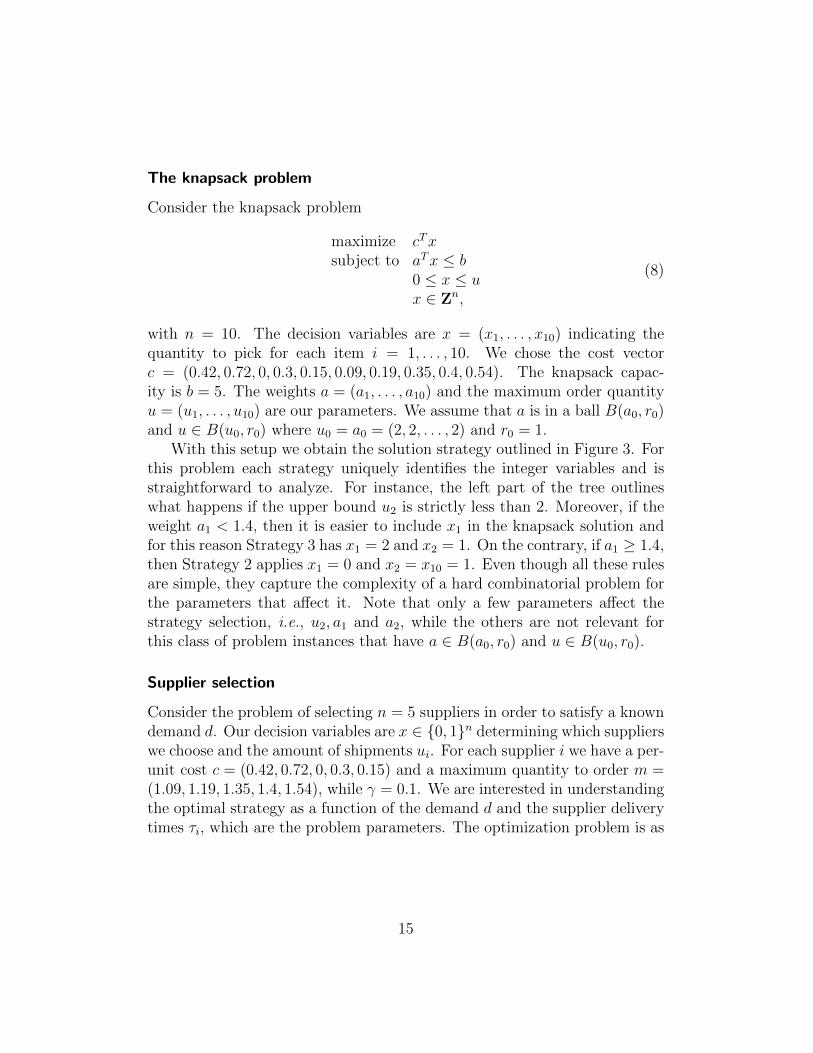
The knapsack problem

Consider the knapsack problem

maximize cTxsubject to aTx ≤ b

0 ≤ x ≤ ux ∈ Zn,

(8)

with n = 10. The decision variables are x = (x1, . . . , x10) indicating thequantity to pick for each item i = 1, . . . , 10. We chose the cost vectorc = (0.42, 0.72, 0, 0.3, 0.15, 0.09, 0.19, 0.35, 0.4, 0.54). The knapsack capac-ity is b = 5. The weights a = (a1, . . . , a10) and the maximum order quantityu = (u1, . . . , u10) are our parameters. We assume that a is in a ball B(a0, r0)and u ∈ B(u0, r0) where u0 = a0 = (2, 2, . . . , 2) and r0 = 1.

With this setup we obtain the solution strategy outlined in Figure 3. Forthis problem each strategy uniquely identifies the integer variables and isstraightforward to analyze. For instance, the left part of the tree outlineswhat happens if the upper bound u2 is strictly less than 2. Moreover, if theweight a1 < 1.4, then it is easier to include x1 in the knapsack solution andfor this reason Strategy 3 has x1 = 2 and x2 = 1. On the contrary, if a1 ≥ 1.4,then Strategy 2 applies x1 = 0 and x2 = x10 = 1. Even though all these rulesare simple, they capture the complexity of a hard combinatorial problem forthe parameters that affect it. Note that only a few parameters affect thestrategy selection, i.e., u2, a1 and a2, while the others are not relevant forthis class of problem instances that have a ∈ B(a0, r0) and u ∈ B(u0, r0).

Supplier selection

Consider the problem of selecting n = 5 suppliers in order to satisfy a knowndemand d. Our decision variables are x ∈ {0, 1}n determining which supplierswe choose and the amount of shipments ui. For each supplier i we have a per-unit cost c = (0.42, 0.72, 0, 0.3, 0.15) and a maximum quantity to order m =(1.09, 1.19, 1.35, 1.4, 1.54), while γ = 0.1. We are interested in understandingthe optimal strategy as a function of the demand d and the supplier deliverytimes τi, which are the problem parameters. The optimization problem is as

15

u2 < 2

a1 < 1.4

3 2

True

a2 < 1.62

4 a2 < 2.48

1 2

False

Figure 3: Example knapsack decision strategies. Strategy 1 : xi = 0 for i 6= 2 andx2 = 2. Strategy 2 : xi = 0 for i 6= 2, 10 and x2 = x10 = 1. Strategy 3 : xi = 0 fori 6= 1, 2 and x1 = 2 and x2 = 1. Strategy 4 : xi = 0 for i 6= 2, 10 and x2 = 2 andx10 = 1.

follows:

minimizen∑

i=1

ciui + γmaxi

({τixi})

subject ton∑

i=1

ui ≥ d

0 ≤ ui ≤ ximi

x ∈ {0, 1}n, ui ∈ R.

(9)

Specifically, we are interested in d ∈ [1, 3] and τ = (τ1, . . . , τ5) ∈ B(τ0, r0)with the center of the ball being τ0 = (2, 3, 2.5, 5, 1) and radius r0 = 0.5.With these parameters we obtain the solution described in Figure 4. Alsoin this case, the decision rules are simple and the solution strategy can beinterpreted from the problem structure. The strategy outputs directly theoptimal choice of suppliers xi and which inequalities are tight correspondingto where we order the maximum quantity, i.e., when ui = mi. Note that thedemand constraint is always tight by construction, i.e., we want to spend theminimum to match d. Therefore, we can fix xi and ui to the values given bythe strategy and we can set the remaining uis to the minimum value suchthat

∑ni=1 ui ≥ d.

In Figure 5, we show the tree that OCT-H gave for this example. Eventhough the accuracy of the OCT in Figure 4 is 100%, the OCT-H depth issmaller at the cost of being less interpretable. Note that in some cases having

16

d < 1.18

τ3 < 2.56

τ5 < 0.79

4 3

τ5 < 1.07

4 3

True

d < 2.89

d < 1.35

3 2

1

False

Figure 4: Example vendor decision strategies using OCT. Strategy 1 : x =(1, 0, 1, 0, 1), u2 = u4 = 0. u3 = m3, u5 = m5 and u1 is left to match demandd. Strategy 2 : x = (0, 0, 1, 0, 1). u1 = u2 = u4 = 0 and u3 = m3. u5 is left tomatch demand d. Strategy 3 : x = (0, 0, 1, 0, 0). u1 = u2 = u4 = u5 = 0 and u3 isleft to match demand d. Strategy 4 : x = (0, 0, 0, 0, 1). u1 = u2 = u3 = u4 = 0. u5is left to match demand d.

a lower depth can make some classification tasks more interpretable despitethe multiple coefficients on the hyperplanes.

3 Machine Learning

In this section, we introduce the core part of our approach: learning the map-ping from parameters to optimal strategies. After the training, the mappingwill replace the core part of standard optimization algorithms – the optimalstrategy search – with a multiclass classification problem where each strategycorresponds to a class label.

3.1 Multiclass Classifier

We would like to solve a multiclass classification problem with i.i.d. data(θi, si), i = 1, . . . , N where θi ∈ Rp are the parameters and si ∈ S thecorresponding labels identifying the optimal strategies. S represents the setof strategies of cardinality |S| = M .

In this work we apply two supervised learning techniques for multiclassclassification to compare their predictive performance: optimal classification

17

d < 1.36

−1.16d+ 0.89τ3 − 0.89τ5 < 1.16

3 4

True

d < 2.89

2 1

False

Figure 5: Example vendor decision strategies using OCT-H. The strategies arethe same as in Figure 4 but accuracy is the same or higher and the tree depth isreduced. Smaller tree depth can sometimes help in interpreting the classification.

trees (OCTs, OCT-Hs) [Bertsimas and Dunn, 2017, 2019] and neural net-works (NNs) [Bengio, 2009, LeCun et al., 2015]. As we mentioned earlierOCTs, OCT-Hs are interpretable and can be described using simple rulesas in the examples in the previous section, while NNs are not interpretablesince they represent a composition of multiple nonlinear functions. A moredetailed description of OCTs and OCT-Hs can be found in Appendix A andof NNs can be found in Appendix B.

3.2 Strategies Exploration

In this section, we estimate how likely it is to find a new parameter θ whoseoptimal strategy does not lie among the ones we have already seen. If wehave already encountered most of the strategies for our problem, then itis unlikely to find unseen strategies. Therefore, we can be sure that ourclassification problem includes all the possible strategies (classes) arising inpractice. Otherwise, we must collect more data to have a more representativeclassification problem.

Estimating the probability of finding unseen strategies. Given N inde-pendent samples ΘN = {θ1, . . . , θN} drawn from an unknown discrete dis-tribution P with the corresponding strategies (s(θ1), . . . , s(θN)), we find Munique strategies S(ΘN) = {s1, . . . , sM}. We are interested in bounding theprobability of finding unseen strategies

P(s(θN+1) /∈ S(ΘN)),

with confidence at least 1− β where β > 0.

18

Historical background. This problem started from the seminal work byTuring and Good [Good, 1953] in the context of decrypting the Enigmacodes during World War II. The Enigma machine was a German navy en-cryption device used for secret military communications. Part of Enigma’sencryption key was a three letter sequence (a word) selected from a bookcontaining all the possible ones in random order. The number of possiblewords was so large that it was impossible to test all the combinations withthe computing power available at that time. In order to decrypt the Enigmamachine without testing all the possible words, Turing wanted to check onlya subset of them while estimating that the likelihood of finding a new unseenword was low. This is how the Good-Turing estimator was developed. Itwas a fundamental step towards the Enigma machine decryption which isbelieved to have shortened World War II of at least two years [Copeland,2012]. In addition, this class of estimators have become standard in a widerange of natural language processing applications.

Good-Turing estimator. Let Nr be the number of strategies that appearedexactly r times in (s(θ1), . . . , s(θN)). The Good-Turing estimator for theprobability of having an unseen strategy is given by Good [1953]

G = N1/N, (10)

which corresponds to the ratio between the number of distinct strategies thathave appeared exactly once, over the total number of samples. Despite theelegant result, Good and Turing did not provide a convergence analysis ofthis estimator for finite samples. Only few decades later the first theoreti-cal work on that topic appeared in [McAllester and Schapire, 2000]. UsingMcDiarmid [1989]’s inequality the authors derived a high probability confi-dence interval. That result can be directly applied to our problem with thefollowing theorem.

Theorem 3.1 (Missing strategies bound). The probability of encounteringa parameter θN+1 corresponding to an unseen strategy s(θN+1) satisfies withconfidence at least 1− β

P(s(θN+1) /∈ S(ΘN)) ≤ G+ c√

(1/N) ln(3/β),

where G corresponds to the Good-Turing estimator (10) and c = (2√

2+√

3).

Proof. The result follows directly from [McAllester and Schapire, 2000, The-orem 9].

19

Exploration algorithm. Given the bound in Theorem 3.1 we construct Al-gorithm 1 to compute the different strategies appearing in our problem. The

Algorithm 1 Strategies exploration

1: given ε, β,Θ = ∅,S = ∅, u =∞2: for k = 1, . . . , do3: Sample θk and compute s(θk) . Sample parameter and strategy.4: Θ← Θ ∪ {θk} . Update set of samples.5: if s(θk) /∈ S then6: S ← S ∪ {s(θk)} . Update strategy set if new strategy found

7: if G+ c√

(1/k) ln(3/β) ≤ ε then . Break if bound less than ε8: break9: return k,Θ,S

algorithm keeps on sampling until we encounter a large enough set of distinctstrategies. It terminates when the probability of encountering a parameterwith an unseen optimal strategy is less than ε with confidence at least 1−β.Note that in practice, instead of sampling one point per iteration k, it is moreconvenient to sample more points to avoid having to recompute the class fre-quencies which becomes computationally intensive with several thousands ofsamples and hundreds of classes. Algorithm 1 imposes no assumptions onthe optimization problem nor the data distribution apart from i.i.d. samples.

4 Machine Learning Optimizer

We implemented our method in the Python software tool MLOPT (MachineLearning Optimizer). It is integrated with CVXPY [Diamond and Boyd,2016] to formulate and solve the problems. CVXPY allows the user to easilydefine mixed-integer convex optimization problems performing all the re-quired reformulations needed by the optimizers while keeping track of theoriginal constraints and variables. This makes it ideal for identifying whichconstraints are tight or not at the optimal solution. The MLOPT implemen-tation is freely available online at

github.com/bstellato/mlopt.

We used the Gurobi Optimizer [Gurobi Optimization, Inc., 2020] tofind the tight constraints because it provides a good tradeoff between

20

Offline

CVXPYModeling

StrategiesSampling

Training

Online

StrategyPrediction

θ s(θ)SolutionDecoding

x?

Figure 6: Algorithm implementation.

solution accuracy and computation time. Note that from Section 2, in caseof LO, MILO, QO and MIQO when the cost f is linear or quadratic andthe constraints g are all linear, the online solution corresponds to solvinga linear system of equations defined by the KKT conditions [Boyd andVandenberghe, 2004, Section 10.2] on the reduced subproblem. This meansthat we can solve those parametric optimization problems without the needto apply any optimization solver.

MLOPT performs the iterative sampling procedure outlined in Section 3.2to obtain the strategies required for the classification task. We sample 5000new points at each iteration and compute their strategies until the GoodTuring estimate is below εGT = 0.005. The strategy computation is fullyparallelized across samples.

We interfaced MLOPT to the machine learning libraries Optimal-Trees.jl [Bertsimas and Dunn, 2019] on multi-core CPUs and PyTorch [Paszkeet al., 2017] for both CPUs and GPUs. In the training phase we automati-cally tune the predictor parameters by splitting the data points in 90%/10%training/validation. We tune the OCTs and OCT-Hs with maximal depthfor values 5, 10, 15 and minimum bucket size for values 1, 5, 10. For theNNs we validate the stochastic gradient descent learning rate for values0.001, 0.01, 0.1, batch size for values 32, 128 and number of epochs for values50, 100. We described the complete algorithm in Figure 6.

21

5 Computational Benchmarks

In this section, we test our approach on multiple examples from continu-ous and mixed-integer optimization. We benchmarked the predictive per-formance of OCTs, OCT-Hs (see Appendix A) and NNs (see Appendix B)depending on the problem type and size. We executed the numerical tests ona Dell R730 cluster with 28 Intel E5-2680 CPUs with a total of 256GB RAMand a Nvidia Tesla K80 GPU. To facilitate the data collection, we generatedthe training samples from distributions on intervals or on hyperballs aroundspecified points. In this way the distributions are unimodal and thereforecloser to the ones encountered in practice. Note that our theoretical resultsdo not assume anything on the distribution generating data apart from i.i.d.samples. Therefore, we could have chosen other distributions such as multi-modal ones. In general, how to generate training data highly depends on thepractical application and in many cases we can simply fit a representativedistribution, either unimodal or multimodal, to the historical data we have.We evaluated the performance metrics on 100 unseen samples drawn fromthe same distribution of θ.

Infeasibility and suboptimality. After the learning phase, we compared thepredicted solution x?i to the optimal one x?i obtained by solving the instancesfrom scratch. Given a parameter θi, we say that the predicted solution isinfeasible if the constraints are violated more than a predefined toleranceεinf = 10−3 according to the infeasibility metric

p(x?i ) = ‖(g(θi, x?i ))+‖2/r(θi, x?i ),

where r(θ, x) normalizes the violation depending on the size of the summandsof g. For example, if g(θ, x) = A(θ)x−b, then r(θ, x) = max(‖A(θ)x‖2, ‖b‖2).If the predicted solution xi is feasible, we define its suboptimality as

d(x?i ) = (f(x?i )− f(x?i ))/|f(x?i )|.

Note that d(x?i ) ≥ 0 by construction. We consider a predicted solution to beaccurate if it is feasible and if the suboptimality is less than the toleranceεsub = 10−3. For each instance we report the maximum infeasibility p =maxi p(x

?i ) and the maximum suboptimality d = maxi d(x?i ) over the test

dataset. Note that for notation ease and to simplify the max operation, if apoint is infeasible we consider its suboptimality 0 and ignore it.

22

Predicting the optimal strategy. Once the learning phase is completed,the predictor outputs the three (3) most likely optimal strategies and picksthe best one according to infeasibility and suboptimality after solving theassociated reduced problems.

Runtimes. The training times of these examples range from a 2 to 12 hoursincluding the time to solve the problems in parallel over the training phaseand the time to train the predictors. Even though this time can be significant,it is comparable to the usual time dedicated to train predictors for modernmachine learning tasks. We report the time ratio tratio between the timeneeded to solve the problem with Gurobi [Gurobi Optimization, Inc., 2020]compared to our method.

Tables notation. We now outline the table headings as reported in everyexample. Dimensions n and/orm denote problem-specific sizes that vary overthe benchmarks. The total number of variables and constraints are nvar andncon respectively. Column “learner” indicates the learner type: OCT, OCT-Hor NN. We indicate the Good-Turing estimator under column “GT” and theaccuracy over the test set as “acc [%]”. The column tratio denotes the speedupof our method over Gurobi [Gurobi Optimization, Inc., 2020]. The maximuminfeasibility appears under column p and the maximum suboptimality undercolumn d.

5.1 Transportation Optimization

Consider a standard transportation problem with n warehouses and m retailstores. Let xij be the quantity we ship from warehouse i to store j. sidenotes the supply for warehouse i and dj the demand from store j. Wedefine the cost of transporting a unit from warehouse i to store j as cij. The

23

optimization problem can be formulated as follows:

minimizen∑

i=1

m∑j=1

cijxij

subject tom∑j=1

xij ≤ si, ∀i

n∑i=1

xij ≥ dj ∀j

xij ≥ 0 ∀i, j.

The first constraint ensures we respect the supply for each warehouse i. Thesecond constraint enforces the sum of all the shipments to match at leastthe demand for store j. Finally, the quantity of shipped product has to benonnegative. Our learning parameters are the demands dj.

Problem instances We generate the transportation problem instances byvarying the number of warehouses n and stores m. The cost vectors ci aredistributed as U(0, 5) and the supplies si as U(3, 13). The parameter vectord = (d1, . . . , dm) was sampled from a uniform distribution within the ballB(d, 0.75) with center d ∼ N (3, 1).

Results. The results appear in Table 1. Independently from the probleminstances the prediction accuracy is very high for both optimal trees andneural networks. Note that even though we solve problems with thousandsof variables and constraints, the number of strategies is always within fewtens or less. The solution time provides usually slight speedups up to almost5 folds. Note that in the very small instances Gurobi can be faster thanour method due to the delays in data exchange between predictor and ourPython code.

5.2 Portfolio Optimization

Consider the problem of allocating assets to minimize the risk adjusted returnconsidered in Markowitz [1952] who formulated it as a QO

maximize µTx− γ(xTΣx)subject to 1Tx = 1

x ≥ 0,

24

Table 1: Transportation benchmarks.

n m nvar ncon learner N GT |S| acc [%] tratio p d

20 20 400 440 NN 10 000 1.00×10−4 11 100.00 0.81 6.34×10−5 4.40×10−16

20 20 400 440 OCT 10 000 1.00×10−4 11 100.00 0.04 6.34×10−5 4.40×10−16

20 20 400 440 OCT-H 10 000 1.00×10−4 11 100.00 1.22 6.34×10−5 4.40×10−16

20 10 200 230 NN 10 000 1.00×10−4 6 100.00 0.74 1.42×10−16 2.76×10−16

20 10 200 230 OCT 10 000 1.00×10−4 6 100.00 0.88 1.42×10−16 2.76×10−16

20 10 200 230 OCT-H 10 000 1.00×10−4 6 100.00 1.36 1.42×10−16 2.76×10−16

40 40 1600 1680 NN 10 000 2.00×10−4 9 100.00 1.95 3.00×10−16 1.98×10−16

40 40 1600 1680 OCT 10 000 2.00×10−4 9 100.00 1.74 3.00×10−16 1.98×10−16

40 40 1600 1680 OCT-H 10 000 2.00×10−4 9 100.00 1.81 3.00×10−16 1.98×10−16

40 20 800 860 NN 10 000 0.00 3 100.00 4.98 1.41×10−16 2.11×10−16

40 20 800 860 OCT 10 000 0.00 3 100.00 3.53 1.41×10−16 2.11×10−16

40 20 800 860 OCT-H 10 000 0.00 3 100.00 3.74 1.41×10−16 2.11×10−16

60 60 3600 3720 NN 10 000 1.50×10−3 43 99.00 2.04 1.86×10−2 2.46×10−16

60 60 3600 3720 OCT 10 000 1.50×10−3 43 95.00 1.80 2.72×10−2 1.55×10−4

60 60 3600 3720 OCT-H 10 000 1.50×10−3 43 100.00 2.11 5.17×10−5 2.46×10−16

60 30 1800 1890 NN 10 000 8.00×10−4 30 99.00 1.70 1.60×10−3 1.97×10−16

60 30 1800 1890 OCT 10 000 8.00×10−4 30 100.00 1.48 1.19×10−16 1.97×10−16

60 30 1800 1890 OCT-H 10 000 8.00×10−4 30 100.00 1.55 1.19×10−16 1.97×10−16

80 80 6400 6560 NN 10 000 1.10×10−3 36 100.00 2.04 1.99×10−16 2.20×10−16

80 80 6400 6560 OCT 10 000 1.10×10−3 36 100.00 2.12 1.99×10−16 2.20×10−16

80 80 6400 6560 OCT-H 10 000 1.10×10−3 36 100.00 2.43 1.99×10−16 2.20×10−16

80 40 3200 3320 NN 10 000 1.00×10−4 14 100.00 2.40 2.10×10−16 3.23×10−16

80 40 3200 3320 OCT 10 000 1.00×10−4 14 100.00 2.13 2.10×10−16 3.23×10−16

80 40 3200 3320 OCT-H 10 000 1.00×10−4 14 100.00 2.38 2.10×10−16 3.23×10−16

25

Table 2: Continuous portfolio benchmarks.

n p ncon learner N GT |S| acc [%] tratio p d

100 10 101 NN 10 000 4.00×10−4 12 100.00 1.01 6.66×10−16 7.06×10−16

100 10 101 OCT 10 000 4.00×10−4 12 100.00 0.09 6.66×10−16 7.06×10−16

100 10 101 OCT-H 10 000 4.00×10−4 12 100.00 1.07 6.66×10−16 7.06×10−16

200 20 201 NN 10 000 4.00×10−4 11 100.00 0.88 4.44×10−16 5.54×10−16

200 20 201 OCT 10 000 4.00×10−4 11 100.00 0.81 4.44×10−16 3.84×10−7

200 20 201 OCT-H 10 000 4.00×10−4 11 100.00 0.79 4.44×10−16 5.54×10−16

300 30 301 NN 10 000 1.00×10−4 4 100.00 2.87 3.38×10−5 6.96×10−16

300 30 301 OCT 10 000 1.00×10−4 4 100.00 2.55 3.38×10−5 6.96×10−16

300 30 301 OCT-H 10 000 1.00×10−4 4 100.00 2.46 3.38×10−5 6.96×10−16

400 40 401 NN 10 000 0.00 14 100.00 1.29 1.48×10−5 5.26×10−16

400 40 401 OCT 10 000 0.00 14 100.00 0.72 1.48×10−5 5.26×10−16

400 40 401 OCT-H 10 000 0.00 14 100.00 1.20 1.48×10−5 1.82×10−7

where the variable x ∈ Rn represents the investments to make.Our learning parameter is the vector of expected returns µ ∈ Rn. In

addition we denote the risk aversion coefficient as γ > 0, and the covariancematrix for the risk model as Σ ∈ Sn

+. Σ is assumed to be

Σ = FF T +D,

where F ∈ Rn×p is the factor loading matrix and D ∈ Rn×n is a diagonalmatrix describing the asset-specific risk.

Problem instances. We generated portfolio instances for different numberof factors p and assets n. We chose the elements of F with 50 % nonzeros andFij ∼ N (0, 1). The diagonal matrix D has elements Dii ∼ U(0,

√p). The

return vector parameters were randomly sampled from a uniform distributionwithin the ball B(µ, 0.15) with µ ∼ N (0, 1). The risk-aversion coefficient isγ = 1.

Results. Results are shown in Table 2. The prediction accuracy for OCTs,OCT-Hs and NNs is 100%, the number of strategies is less than 15, and theinfeasibility and suboptimality are very low. The solution times improvementis not significant due to the delays of passing data to the predictor and thefact that Gurobi is fast for these problems.

26

5.3 Facility location

Let i ∈ I the set of possible locations for facilities such as factories or ware-houses. We denote as j ∈ J the set of delivery locations. The cost oftransporting a unit of goods from facility i to location j is cij. The con-struction cost for building facility i is fi. For each location j, we define thedemand dj. The capacity of facility i is si. The main goal of this problemis to find the best tradeoff between transportation costs versus constructioncosts. We can write the model as a MILO

minimize∑i∈I

∑j∈J

cijxij +∑i∈I

fiyi

subject to∑i∈I

xij ≥ dj, ∀j ∈ J∑j∈J

xij ≤ siyi, ∀i ∈ I

xij ≥ 0yi ∈ {0, 1}.

(11)

The decision variables xij describe the amount of goods sent from facility ito location j. The binary variables yi determine if we build facility i or not.

Problem instances. We generated the facility location instances for differ-ent values of facilities n and warehouses m. The costs cij are sampled from auniform distribution U(0, 1) and fi from U(0, 10). We chose capacities si asU(8, 18) to ensure the problem is always feasible. The demands parametersd = (d1, . . . , dm) were sampled from a uniform distributions within the ballB(d, 0.25) with d ∼ N (3, 1).

Results. Table 3 shows the benchmark examples. All prediction methodsshowed very high accuracy. There is a significant improvement in computa-tion time compared to Gurobi. To illustrate an example of the OCT inter-pretability, we reported the resulting tree for n = 60 and m = 30 in Figure 7.Even though for space concerns we cannot directly report the strategies interms of tight constraints and integer variables since the problem involves1860 variables and 2010 constraints, the tree is remarkably simple. In everystrategy all the demand constraints are tight since we are trying to minimizethe cost while satisfying the demand. In addition, the strategy illustrateswhich facilities hit the maximum capacity si which could mean that further

27

Table 3: Facility location benchmarks.

n m nvar ncon learner N GT |S| acc [%] tratio p d

20 10 220 270 NN 10 000 0.00 1 100.00 537.67 1.06×10−16 1.64×10−16

20 10 220 270 OCT 10 000 0.00 1 100.00 3.87 1.06×10−16 1.64×10−16

20 10 220 270 OCT-H 10 000 0.00 1 100.00 573.24 1.06×10−16 1.64×10−16

20 20 420 480 NN 10 000 1.00×10−4 9 100.00 149.06 9.45×10−5 1.81×10−9

20 20 420 480 OCT 10 000 1.00×10−4 9 100.00 174.62 9.45×10−5 1.81×10−9

20 20 420 480 OCT-H 10 000 1.00×10−4 9 100.00 234.11 9.45×10−5 1.81×10−9

40 20 840 940 NN 10 000 0.00 2 100.00 1986.00 1.76×10−16 2.43×10−16

40 20 840 940 OCT 10 000 0.00 2 100.00 2080.12 1.76×10−16 2.43×10−16

40 20 840 940 OCT-H 10 000 0.00 2 100.00 2201.23 1.76×10−16 2.43×10−16

40 40 1640 1760 NN 10 000 1.00×10−4 5 100.00 1037.03 1.42×10−16 2.50×10−9

40 40 1640 1760 OCT 10 000 1.00×10−4 5 100.00 961.91 1.42×10−16 2.50×10−9

40 40 1640 1760 OCT-H 10 000 1.00×10−4 5 100.00 1070.20 1.42×10−16 2.50×10−9

60 30 1860 2010 NN 10 000 1.00×10−4 3 100.00 325.76 2.02×10−16 1.91×10−16

60 30 1860 2010 OCT 10 000 1.00×10−4 3 100.00 334.58 2.02×10−16 1.91×10−16

60 30 1860 2010 OCT-H 10 000 1.00×10−4 3 100.00 296.36 2.02×10−16 1.91×10−16

60 60 3660 3840 NN 10 000 1.00×10−4 5 100.00 341.24 3.01×10−16 2.63×10−16

60 60 3660 3840 OCT 10 000 1.00×10−4 5 100.00 415.54 3.01×10−16 2.63×10−16

60 60 3660 3840 OCT-H 10 000 1.00×10−4 5 100.00 409.08 3.01×10−16 2.63×10−16

80 40 3280 3480 NN 10 000 1.00×10−4 9 100.00 97.38 3.03×10−16 2.77×10−16

80 40 3280 3480 OCT 10 000 1.00×10−4 9 100.00 99.44 3.03×10−16 2.77×10−16

80 40 3280 3480 OCT-H 10 000 1.00×10−4 9 100.00 89.52 3.03×10−16 2.77×10−16

80 80 6480 6720 NN 10 000 1.00×10−4 6 100.00 865.45 3.34×10−16 2.52×10−10

80 80 6480 6720 OCT 10 000 1.00×10−4 6 100.00 64.74 3.34×10−16 2.52×10−10

80 80 6480 6720 OCT-H 10 000 1.00×10−4 6 100.00 1061.22 3.34×10−16 2.52×10−10

facilities might be needed in that area. Finally, with the values of binaryvariables yi, the strategy tells us which facilities we should open dependingon the demand.

5.4 Hybrid Vehicle Control

Consider the hybrid-vehicle control problem in [Takapoui et al., 2017, Sec-tion 3.2]. The model consists of a battery, an electric motor/generator andan engine. We assume to know the demanded power P des

t over the horizont = 0, . . . , T − 1. The goal is to plan the battery and the engine poweroutputs P batt

t and P engt so that they match at least the demand,

P battt + P eng

t ≥ P dest .

The status of the battery is modeled with the internal energy Et evolving as

Et+1 = Et − τP battt ,

28

d8 < 3.35

d18 < 3.04

1 d30 < 2.19

2 d18 < 3.04

2 1

False

1

True

Figure 7: Facility location benchmark OCT for n = 60 and m = 30.

where τ > 0 is the time interval discretization. The battery capacity islimited by Emax and its initial value is Einit.

We now model the cost function. We penalize the terminal energy stateof the battery with the function

g(E) = η(Emax − E)2.

with η ≥ 0. At each time t we model the on-off state of the engine with thebinary variable zt. When the engine is off (zt = 0) we do not consume anyenergy, thus we have 0 ≤ P eng

t ≤ Pmaxzt. When the engine is on (zt = 1) itconsumes αP eng

t + βP engt + γ units of fuel, with α, β, γ > 0. We define the

stage power cost asf(P, z) = αP 2 + βP + γz.

We also introduce a cost of turning the engine on at time t as δ(zt − zt−1)+.The hybrid vehicle control problem can be formulated as a mixed integer

29

quadratic optimization problem:

minimize η(ET − Emax)2 +T−1∑t=0

f(P engt , zt) + δ(zt − zt−1)+

subject to Et+1 = Et − τP battt , t = 0, . . . , T − 1

0 ≤ Et ≤ Emax, t = 0, . . . , TE0 = Einit

0 ≤ P engt ≤ Pmax, t = 0, . . . , T − 1

P battt + P eng

t ≥ P dest , t = 0, . . . , T − 1

zt ∈ {0, 1}, t = 0, . . . , T − 1.

The initial state E0 and demanded power P dest are our parameters.

Problem instances. We generated the control instances with varying hori-zon length T . The discretization time interval is τ = 4. We chose the costfunction parameters α = β = γ = 1, and δ = 0.1. The maximum charge isEmax = 50 and the maximum power Pmax = 1. The parameter E0 was sam-pled from a uniform distribution within the ball B(40, 0.5). The demand P des

also comes from a uniform distribution within the ball B(Pdes, 0.5) where

Pdes

t = (0.05, 0.30, 0.55, 0.80, 1.05, 1.30, 1.55, 1.80, 1.95, 1.70, 1.45, 1.20, 1.02,

1.12, 1.22, 1.32, 1.42, 1.52, 1.62, 1.72, 1.73, 1.38, 1.03, 0.68, 0.33,−0.02,

− 0.37,−0.72,−0.94,−0.64,−0.34,−0.04, 0.18, 0.08,−0.02,−0.12,

− 0.22,−0.32,−0.42,−0.52)

is the desired power in Takapoui et al. [2017]. Depending on the horizon

length T we choose only the first T elements of Pdes

to sample P des.

Results. We present the results in Table 4. Here there is a significantimprovement in computation time compared to Gurobi. Also in this casethe number of strategies |S| is much less than the number of variables or theworst case number of control input combinations. The maximum infeasibilityand suboptimality are low even when the predictions are not exact and theperformance of OCTs, OCT-Hs and NNs is comparable except in the lastcase.

30

Table 4: Hybrid control benchmarks.

T nvar ncon learner N GT |S| acc [%] tratio p d

10 51 103 NN 10 000 3.00×10−4 16 100.00 2.79 1.17×10−14 3.78×10−15

10 51 103 OCT 10 000 3.00×10−4 16 99.00 0.12 9.37×10−4 3.78×10−15

10 51 103 OCT-H 10 000 3.00×10−4 16 100.00 3.00 1.17×10−14 3.78×10−15

15 76 153 NN 10 000 4.00×10−4 16 99.00 4.20 7.27×10−5 4.29×10−15

15 76 153 OCT 10 000 4.00×10−4 16 99.00 3.68 7.27×10−5 4.29×10−15

15 76 153 OCT-H 10 000 4.00×10−4 16 99.00 3.05 7.27×10−5 4.29×10−15

20 101 203 NN 10 000 6.00×10−4 16 100.00 3.89 1.46×10−14 6.04×10−15

20 101 203 OCT 10 000 6.00×10−4 16 99.00 4.16 2.23×10−4 6.04×10−15

20 101 203 OCT-H 10 000 6.00×10−4 16 100.00 4.33 1.46×10−14 6.04×10−15

25 126 253 NN 10 000 2.00×10−4 10 100.00 4.27 5.49×10−5 6.33×10−15

25 126 253 OCT 10 000 2.00×10−4 10 100.00 4.38 5.49×10−5 6.33×10−15

25 126 253 OCT-H 10 000 2.00×10−4 10 100.00 5.12 5.49×10−5 6.33×10−15

30 151 303 NN 10 000 1.00×10−4 20 100.00 86.65 1.55×10−13 7.72×10−16

30 151 303 OCT 10 000 1.00×10−4 20 100.00 148.37 1.55×10−13 7.72×10−16

30 151 303 OCT-H 10 000 1.00×10−4 20 100.00 124.01 1.55×10−13 7.72×10−16

35 176 353 NN 10 000 3.00×10−4 37 100.00 845.13 4.04×10−5 1.14×10−15

35 176 353 OCT 10 000 3.00×10−4 37 98.00 1010.73 4.04×10−5 3.48×10−4

35 176 353 OCT-H 10 000 3.00×10−4 37 100.00 1250.19 4.04×10−5 5.98×10−5

40 201 403 NN 10 000 2.00×10−4 35 100.00 6461.46 6.50×10−14 1.53×10−15

40 201 403 OCT 10 000 2.00×10−4 35 93.00 6846.49 6.50×10−14 3.12×10−2

40 201 403 OCT-H 10 000 2.00×10−4 35 89.00 6551.66 6.50×10−14 3.02×10−2

31

6 Conclusions

We introduced the idea that using OCTs and OCT-Hs we obtain insighton the strategy of the optimal solution in many optimization problems asa function of key parameters. In this way, optimization is not a black boxanymore, but rather it has a voice, i.e., we are able to provide insights onthe logic behind the optimal solution. The class of optimization problemsthat these ideas apply to is rather broad since it includes any continuousand mixed-integer convex optimization problems without any assumption onthe parameters dependency. The accuracy of our approach is in the 90%-100%, while even when it does not provide the optimal solution the degree ofsuboptimality or infeasibility is extremely low. In addition, the computationtimes of our method are significantly faster than solving the problem usingstandard optimization algorithms. Even though the solving times did nothave a strict limit for the proposed applications, our method can be usefulin online settings where problems must be solved within a limited time andwith limited computational resources. Applications of this framework to fastonline optimization appear in [Bertsimas and Stellato, 2019]. Comparisons onseveral examples show that the out-of-sample strategy prediction accuracy ofOCT-Hs is comparable to the NNs. OCTs show competitive accuracy in mostcomparisons apart from the cases with higher number of strategies where theprediction performance degrades. Note that this is not necessarily related tothe size of the problem but rather to how the parameters affect the optimalsolution and, in turn, the total number of strategies. OCTs also exhibit lowinfeasibility and low suboptimality even when the prediction is not correct. Inaddition, OCTs have higher interpretability than OCT-Hs and NNs becauseof their structure with parallel splits, therefore, being required in applicationswhere models must be explainable. For these reasons, our framework providesa reliable and insightful understanding of optimal solutions in a broad classof optimization problems using different machine learning algorithms.

A Optimal Classification Trees

OCTs and OCT-Hs developed by Bertsimas and Dunn [2017, 2019] are a re-cently proposed generalization of classification and regression trees (CARTs)developed by Breiman et al. [1984] that construct decision trees that arenear optimal with significantly higher prediction accuracy while retaining

32

their interpretability. Bertsimas et al. [2018] have shown that given a NN(feedforward, convolutional and recurrent), we can construct an OCT-H thathas the same in sample accuracy, that is OCT-Hs are at least as powerful asNNs. The constructions can sometimes generate OCT-Hs with high depth.However, they also report computational results that show that OCT-Hs andNNs have comparable performance in practice even for depths of OCT-Hsbelow 10.

Architecture. OCTs recursively partition the feature space Rp to constructhierarchical disjoint regions. A tree can be defined as a set of nodes t ∈ T oftwo types T = TB ∪ TL:

Branch nodes Nodes t ∈ TB at the tree branches describe a split of theform aTt θ < bt where at ∈ Rp and bt ∈ R. They partition the space intwo subsets: the points on the left branch satisfying the inequality andthe remaining ones points on the right branch. If splits involve a singlevariable we denote them as parallel and we refer to the tree as optimalclassification tree (OCT). This is achieved by enforcing all componentsof at to be all 0 except from one. Otherwise, if the components of atcan be freely nonzero, we denote the splits as hyperplanes and we referto the tree as optimal classification tree with-hyperplanes (OCT-H).

Leaf nodes Nodes t ∈ TL at the tree leaves make a class prediction for eachpoint falling into that node.

An example OCT for the Iris dataset appears in Figure 8 [Bertsimas andDunn, 2019]. For each new data point it is straightforward to follow whichhyperplanes are satisfied and to make a prediction. This characteristic makesOCTs and OCT-Hs highly interpretable. Note that the level of interpretabil-ity of the resulting trees can be also tuned by changing minimum sparsity ofat. The two extremes are maximum sparsity OCTs and minimum sparsityOCT-Hs but we can specify anything in between.

Learning. With the latest computational advances in MIO, Bertsimas andDunn [2019] were able to exactly formulate the tree training as a MIO prob-lem and solve it in a reasonable amount of time for problem sizes arising inreal-world applications.

33

PetalLength < 2.45

Setosa

True

PetalWidth < 1.75

PetalLength < 4.95

Versicolor Virginica

Virginica

False

Figure 8: Example OCT for the Iris dataset Bertsimas and Dunn [2019].

The OCT cost function is a tradeoff between the misclassification errorat each leaf and the tree complexity

LOCT =∑t∈TL

Lt + α∑t∈TB

‖at‖1,

where the Lt is the misclassification error at node t and the second termrepresents the complexity of the tree measured as the sum of the norm ofthe hyperplane coefficients in all the splits. The parameter α > 0 regulatesthe tradeoff. For more details about the cost function and the constraints ofthe problem, we refer the reader to [Bertsimas and Dunn, 2019, Section 2.2,Section 3.1].

Bertsimas and Dunn apply a local search method [Bertsimas and Dunn,2019, Section 2.3] that manages to solve OCT problems for realistic sizes infraction of the time an off-the-shelf optimization solver would take. The algo-rithm proposed iteratively improves and refines the current tree until a localminimum is reached. By repeating this search from different random initial-ization points the authors compute several local minima and then take thebest one as the resulting tree. This heuristic showed remarkable performanceboth in terms of computation time and quality of the resulting tree becomingthe algorithm included in the OptimalTrees.jl Julia package [Bertsimas andDunn, 2019].

34

B Neural Networks

NNs have recently become one of the most prominent machine learning tech-niques revolutionizing fields such as speech recognition [Hinton et al., 2012]and computer vision [Krizhevsky et al., 2012]. The wide range of applica-tions of these techniques recently extended to autonomous driving [Bojarskiet al., 2016] and reinforcement learning [Silver et al., 2017]. The popularityof neural networks is also due to the widely used open-source libraries learn-ing on CPUs and GPUs coming from both academia and industry such asTensorFlow [Abadi et al., 2015], Caffe [Jia et al., 2014] and PyTorch [Paszkeet al., 2017]. We use feedforward neural networks which offer a good tradeoffbetween simplicity and accuracy without resorting to more complex archi-tectures such as convolutional or recurrent neural networks [LeCun et al.,2015].

Architecture. Given L layers, a neural network is a composition of func-tions of the form

s = fL(fL−1(. . . f1(θ))),

where each function consists of

yl = f(yl−1) = g(Wlyl−1 + bl). (12)

The number of nodes in each layer is nl and corresponds to the dimension ofthe vector yl ∈ Rnl . Layer l = 1 is defined as the input layer and l = L asthe output layer. Consequently y1 = θ and yL = s. The linear transforma-tion in each layer is composed of an affine transformation with parametersWl ∈ Rnl×nl−1 and bl ∈ Rnl . The activation function g : Rnl → Rnl mod-els nonlinearities. We chose as activation function the rectified linear unit(ReLU) defined as

g(x) = max(x, 0),

for all the layers l = 1, . . . , L − 1. Note that the max operator is intendedelement-wise. We chose a ReLU because on the one hand it provides sparsityto the model since it is 0 for the negative components of x and because onthe other hand it does not suffer from the vanishing gradient issues of thestandard sigmoid functions [Goodfellow et al., 2016]. An example neuralnetwork can be found in Figure 9.

For the output layer we would like the network to output not only thepredicted class, but also a normalized ranking between them according to

35

f1θ

f2y1 y2 . . . fL

yL−1 s

Figure 9: Example Feedforward Neural Network with functions fi, i = 1, . . . , Ldefined in (12).

how likely they are to be the right one. This can be achieved with a softmaxactivation function in the output layer defined as

g(x)j =exj∑Mj=1 e

xj

,

where j = 1, . . . ,M are the elements of g(x). Hence, 0 ≤ g(x) ≤ 1 and thepredicted class is argmax(s).

Learning. Before training the network, we rewrite the labels for the neuralnetwork learning using a one-hot encoding, i.e., si ∈ RM where M is the totalnumber of classes and all the elements of si are 0 except the one correspondingto the class which is 1.

We define a smooth cost function amenable to algorithms such as gradientdescent, i.e., the cross-entropy loss

LNN =N∑i=1

−sTi log(si),

where log is intended element-wise. The cross-entropy loss L can also beinterpreted as the distance between the predicted probability density of thelabels compared to the true one.

The actual training phase consists of applying stochastic gradient descentusing the derivatives of the cost function using the back-propagation rule.This method works very well in practice and provides good out-of-sampleperformance with short training times.

References

M. Abadi, A. Agarwal, P. Barham, E. Brevdo, Z. Chen, C. Citro, G. S. Cor-rado, A. Davis, J. Dean, M. Devin, S. Ghemawat, I. Goodfellow, A. Harp,

36

G. Irving, M. Isard, Y. Jia, R. Jozefowicz, L. Kaiser, M. Kudlur, J. Lev-enberg, D. Mane, R. Monga, S. Moore, D. Murray, C. Olah, M. Schus-ter, J. Shlens, B. Steiner, I. Sutskever, K. Talwar, P. Tucker, V. Van-houcke, V. Vasudevan, F. Viegas, O. Vinyals, P. Warden, M. Wattenberg,M. Wicke, Y. Yu, and X. Zheng. TensorFlow: Large-scale machine learningon heterogeneous systems, 2015. URL https://www.tensorflow.org/.Software available from tensorflow.org.

A. M. Alvarez, Q. Louveaux, and L. Wehenkel. A machine learning-basedapproximation of strong branching. INFORMS Journal on Computing, 29(1):185–195, 2017.

Y. Bengio. Learning deep architectures for AI. Foundations and Trends inMachine Learning, 2(1):1–127, 2009. ISSN 1935-8237.

Y. Bengio, A. Lodi, and A. Prouvost. Machine learning for combinatorialoptimization: a methodological tour d’horizon. arXiv:1811.0612, 2018.

D. Bertsimas and J. Dunn. Optimal classification trees. Machine Learning,106(7):1039–1082, July 2017. ISSN 1573-0565.

D. Bertsimas and J. Dunn. Machine Learning under a Modern OptimizationLens. Dynamic Ideas Press, 2019.

D. Bertsimas and B. Stellato. Online mixed-integer optimization in millisec-onds. arXiv:1907.02206, 2019.

D. Bertsimas and J. N. Tsitsiklis. Introduction to Linear Optimization.Athena Scientific, 1997. ISBN 978-1-886529-19-9.

D. Bertsimas, R. Mazumder, and M.. Sobiesk. Optimal classification andregression trees with hyperplanes are as powerful as classification and re-gression neural networks. (submitted for publication), 2018.

M. Bojarski, D. Del Testa, D. Dworakowski, B. Firner, B. Flepp, P. Goyal,L. D. Jackel, M. Monfort, U. Muller, J. Zhang, X. Zhang, J. Zhao, andK. Zieba. End to end learning for self-driving cars. arXiv:1604.17316, 2016.

P. Bonami, A. Lodi, and G. Zarpellon. Learning a classification of mixed-integer quadratic programming problems. In Willem-Jan van Hoeve, ed-itor, Integration of Constraint Programming, Artificial Intelligence, and

37

Operations Research, pages 595–604, Cham, 2018. Springer InternationalPublishing.

S. Boyd and L. Vandenberghe. Convex Optimization. Cambridge UniversityPress, 2004.

L. Breiman, J. H. Friedman, R. A. Olshen, and C. J. Stone. Classification andregression trees. The Wadsworth statistics/probability series. Wadsworth& Brooks/Cole Advanced Books & Software, Monterey, CA, 1984.

G. C. Calafiore. Random convex programs. SIAM Journal on Optimization,20(6):3427–3464, jan 2010.

E. Clarke, A. Gupta, J. Kukula, and O. Strichman. SAT based abstraction-refinement using ILP and machine learning techniques. In E. Brinksmaand K. G. Larsen, editors, Computer Aided Verification, pages 265–279,Berlin, Heidelberg, 2002. Springer Berlin Heidelberg.

J. Copeland. Alan Turing: The codebreaker who saved ’millions oflives’. BBC News, June 2012. URL https://www.bbc.com/news/

technology-18419691. [Online; posted 19-June-2012].

H. Dai, E. B. Khalil, Y. Zhang, B. Dilkina, and L. Song. Learning combina-torial optimization algorithms over graphs. arXiv:1704.01665, 2017.

H.un Dai, B. Dai, and L. Song. Discriminative embeddings of latent vari-able models for structured data. In Proceedings of the 33rd InternationalConference on International Conference on Machine Learning - Volume48, ICML’16, pages 2702–2711. JMLR.org, 2016.

S. Diamond and S. Boyd. CVXPY: A Python-embedded modeling languagefor convex optimization. Journal of Machine Learning Research, 17(83):1–5, 2016.

I. J. Good. The population frequencies of species and the estimation of pop-ulation parameters. Biometrika, 40(3/4):237–264, 1953. ISSN 00063444.

I. Goodfellow, Y. Bengio, and A. Courville. Deep Learning. MIT Press, 2016.

Gurobi Optimization, Inc. Gurobi optimizer reference manual, 2020. URLhttp://www.gurobi.com.

38

T. Hastie, R. Tibshirani, and J. Friedman. The Elements of Statistical Learn-ing. Number 2 in Springer Series in Statistics. Springer-Verlag New York,2009. ISBN 978-0-387-84858-7.

G. Hinton, L. Deng, D. Yu, G. E. Dahl, A. Mohamed, N. Jaitly, A. Senior,V. Vanhoucke, P. Nguyen, T. N. Sainath, and B. Kingsbury. Deep neuralnetworks for acoustic modeling in speech recognition: The shared views offour research groups. IEEE Signal Processing Magazine, 29(6):82–97, Nov2012. ISSN 1053-5888.

A. J. Hoffman. BINDING CONSTRAINTS AND HELLY NUMBERS. An-nals of the New York Academy of Sciences, 319(1 Second Intern):284–288,may 1979.

F. Hutter, H. H. Hoos, K. Leyton-Brown, and T. Stutzle. ParamILS: Anautomatic algorithm configuration framework. Journal of Artificial Intel-ligence Research, 36(1):267–306, September 2009.

F. Hutter, H. H. Hoos, and K. Leyton-Brown. Sequential model-based op-timization for general algorithm configuration. In C. A. Coello, editor,Learning and Intelligent Optimization, pages 507–523, Berlin, Heidelberg,2011. Springer Berlin Heidelberg.

Y. Jia, E. Shelhamer, J. Donahue, S. Karayev, J. Long, R. Girshick,S. Guadarrama, and T. Darrell. Caffe: Convolutional architecture forfast feature embedding. arXiv:1408.5093, 2014.

E. B. Khalil, P. L. Bodic, L. Song, G. Nemhauser, and B. Dilkina. Learningto branch in mixed integer programming. In Proceedings of the Thir-tieth AAAI Conference on Artificial Intelligence, AAAI’16, pages 724–731. AAAI Press, 2016. URL http://dl.acm.org/citation.cfm?id=

3015812.3015920.

M. Klauco, M. Kaluz, and M. Kvasnica. Machine learning-based warm start-ing of active set methods in embedded model predictive control. Engineer-ing Applications of Artificial Intelligence, 77:1 – 8, 2019. ISSN 0952-1976.

A. Krizhevsky, I. Sutskever, and G. E. Hinton. Imagenet classification withdeep convolutional neural networks. In Advances in Neural InformationProcessing Systems, page 2012, 2012.

39

M. Kruber, M. E. Lubbecke, and A. Parmentier. Learning when to use adecomposition. In Domenico Salvagnin and Michele Lombardi, editors,Integration of AI and OR Techniques in Constraint Programming, pages202–210, Cham, 2017. Springer International Publishing.

Y. LeCun, Y. Bengio, and G. Hinton. Deep learning. Nature, 521(7553):436–444, may 2015.

M. Lopez-Ibanez, J. Dubois-Lacoste, L. Perez Caceres, M. Birattari, andT. Stutzle. The irace package: Iterated racing for automatic algorithmconfiguration. Operations Research Perspectives, 3:43 – 58, 2016.

H. Markowitz. Portfolio selection. The Journal of Finance, 7(1):77–91, 1952.ISSN 1540-6261.

D. A. McAllester and R. E. Schapire. On the convergence rate of Good-Turing estimators. In Proceedings of the 13th Annual Conference on Com-putational Learning Theory, 2000.

C. McDiarmid. On the method of bounded differences, pages 148–188. LondonMathematical Society Lecture Note Series. Cambridge University Press,1989.

S. Minton. Automatically configuring constraint satisfaction programs: Acase study. Constraints, 1(1–2):7–43, 1996.

S. Misra, L. Roald, and Y. Ng. Learning for constrained optimization: Iden-tifying optimal active constraint sets. arXiv:1802.09639v4, 2019.

A. Paszke, S. Gross, S. Chintala, G. Chanan, E. Yang, Z. DeVito, Z. Lin,A. Desmaison, L. Antiga, and A. Lerer. Automatic differentiation in Py-Torch. In NIPS-W, 2017.

D. Selsam, M. Lamm, B. Bunz, P. Liang, L. de Moura, and D. L. Dill. Learn-ing a SAT solver from single-bit supervision. In International Conferenceon Learning Representations, 2019.

D. Silver, J. Schrittwieser, K. Simonyan, I. Antonoglou, A. Huang, A. Guez,T. Hubert, L. Baker, M. Lai, A. Bolton, Y. Chen, L. Lillicrap, F. Hui,L. Sifre, G. van den Driessche, T. Graepel, and D. Hassabis. Masteringthe game of go without human knowledge. Nature, 550(7676):354–359, oct2017.

40

K. A. Smith. Neural networks for combinatorial optimization: A review ofmore than a decade of research. INFORMS Journal on Computing, 11(1):15–34, 1999.

R. S. Sutton and A. G. Barto. Reinforcement Learning: An Introduction. ABradford Book, 2nd edition, 2018.

R. Takapoui, N. Moehle, S. Boyd, and A. Bemporad. A simple effectiveheuristic for embedded mixed-integer quadratic programming. Interna-tional Journal of Control, pages 1–11, 2017.

L. Xu, F. Hutter, H. H. Hoos, and K. Leyton-Brown. SATzilla: Portfolio-based algorithm selection for SAT. Journal of Artificial Intelligence Re-search, 32(1):565–606, June 2008. ISSN 1076–9757.

Y.-S. Zheng and A. Federgruen. Finding optimal (s, S) policies is about assimple as evaluating a single policy. Operations Research, 39(4):654–665,1991.

41