The Varieties of Rentier Experience: How Natural Resource Endowments Affect the Political Economy of Economic Growth*

Jonathan Isham Michael Woolcock

Middlebury College World Bank

Lant Pritchett Gwen Busby Harvard University Yale University

This draft: January 8, 2002

Abstract: Many oil- and mineral-rich countries have not fared well since the oil shock of the early 1970s. This paper tests the hypothesis that a developing country’s natural resource endowment affects economic growth through its influence on socioeconomic and political institutions. The paper’s thesis is that different export structures—whether foreign exchange is derived primarily from manufactures, diffuse natural resources, point-source natural resources, or coffee/cocoa natural resources—create differential institutional capacities to manage shocks and reduce social and economic divisions in developing countries. Using one new and one established measure of natural resource abundance as exogenously-determined instruments, we find evidence to support the hypotheses that countries that are abundant (scarce) in point-source natural resources have weaker (stronger) institutional capacities; and that these endogenously determined institutional capacities are significant and large determinants of growth since the oil shock. Specifically, three-stage least-squares estimates show that (a) being a point-source economy is associated with having worse institutions (at least a one standard deviation decrease); and (b) having worse institutions translates into a GPD per capita that, 25 years after the oil shock, is almost 33 percent lower than countries with better institutions.

Keywords: economic growth, institutions, natural resource endowment JEL Codes: 013; 050; Z13

* We thank William Easterly, Dani Kaufmann, and Michael Ross for their rapid and informative sharing of data and ideas, and Richard Auty and Jean-Philippe Stijns for useful comments. We also thank the Department of Economics and the Program in Environmental Studies at Middlebury College for research support. An earlier version of this paper (Woolcock, Isham, and Pritchett 2001) was prepared for—and benefited from discussions among other contributors to—the UNU/WIDER Project on Resource Abundance and Economic Growth. Please address comments to jisham@middlebury.edu and mwoolcock@worldbank.org

2

The rentier state is a state of parasitic, decaying capitalism, and this circumstance cannot fail to influence all the socio-political conditions of the countries concerned. Vladimir Lenin, Imperialism, the Highest Stage of Capitalism1 It matters whether a state relies on taxes from extractive industries, agricultural production, foreign aid, remittances, or international borrowing because these different sources of revenues, whatever their relative economic merits or social import, have powerful (and quite different) impact on the state’s institutional development and its abilities to employ personnel, subsidize social and economic programs, create new organizations, and direct the activities of private interests. Simply stated, the revenues a state collects, how it collects them, and the uses to which it puts them define its nature.

Terry Karl, The Paradox of Plenty2

I. Introduction

In recent years, many researchers have weighed in with explanations for the big differences in

growth performance from the mid-1970s to the mid-1990s among economies with different

natural resource bases (see, among others, Auty 1995; Leamer et al 1999; Leite and Weidmann

1999; Ross 1999, 2001; Sachs and Warner 1995 [2000], 1999; Stijns 2001). Woolcock, Pritchett

and Isham (2001) hypothesized that the differential capacity to handle growth collapses among

economies with different types of export revenue streams—manufacturing, “point source”

natural resources (e.g., oil, diamonds, plantation crops), “diffuse” natural resources (e.g., wheat,

rice, animals), or coffee/cocoa—is largely a function of varying socioeconomic and political

institutions. This paper presents new econometric evidence to support this hypothesis.

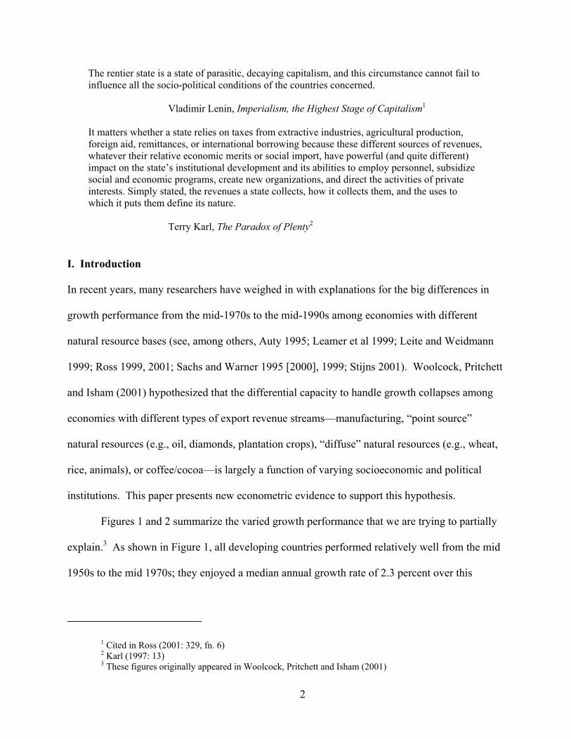
Figures 1 and 2 summarize the varied growth performance that we are trying to partially

explain.3 As shown in Figure 1, all developing countries performed relatively well from the mid

1950s to the mid 1970s; they enjoyed a median annual growth rate of 2.3 percent over this

1 Cited in Ross (2001: 329, fn. 6) 2 Karl (1997: 13) 3 These figures originally appeared in Woolcock, Pritchett and Isham (2001)

3

period. From the mid 1970s until the mid 1990s, by contrast, developing economies endured a

growth collapse of “Grand Canyon” proportions, setting back their development agenda by at

least a decade.

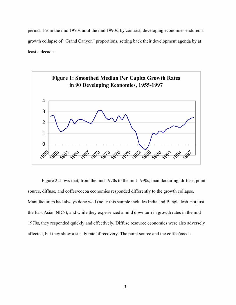
Figure 2 shows that, from the mid 1970s to the mid 1990s, manufacturing, diffuse, point

source, diffuse, and coffee/cocoa economies responded differently to the growth collapse.

Manufacturers had always done well (note: this sample includes India and Bangladesh, not just

the East Asian NICs), and while they experienced a mild downturn in growth rates in the mid

1970s, they responded quickly and effectively. Diffuse resource economies were also adversely

affected, but they show a steady rate of recovery. The point source and the coffee/cocoa

Figure 1: Smoothed Median Per Capita Growth Rates in 90 Developing Economies, 1955-1997

-1

0

1

2

3

4

1955

1958

1961

1964

1967

1970

1973

1976

1979

1982

1985

1988

1991

1994

1997

4

economies, however, experienced a protracted growth collapse. Why?

Our contribution in this paper is to show how the profile of a country’s sources of export

revenue—i.e., how a country earns its living and pays its bills—affects economic growth. We

show that a profile with a bias towards point-source natural resources such as oil, minerals, and

plantation crops is strongly associated with societal division and weak public institutions which,

in turn, are strongly associated with slower growth.

The rest of this paper is organized as follows. Section II summarizes some recent

relevant headlines, details our hypothesis, and motivates the test of our central hypothesis with

some illustrative cross-tabulations. Section III presents our econometric model and summarizes

the available data for testing the model. Section IV presents our main empirical results, and

Section V presents various robustness checks of these results. Section V discusses and

concludes.

Figure 2: Smoothed Median Growth Rates for 90 Developing Economies, 1957-1997

-3-2-101234567

1957

1961

1965

1969

1973

1977

1981

1985

1989

1993

1997

Diffuse (N=18)

Point Source(N=45)Coffee/Cocoa(N=18)Manufacturing(N=9)

5

II: Development of our hypothesis

A. Cases to ponder

Here are examples to illustrate what we are try to get at in this paper, and the difficulties with

adopting a single or simplistic view of the relationship between natural resources and economic

growth.

Some have argued that resource scarcity is behind civil conflicts in Africa (e.g., Klare,

2001), asserting for instance that a major explanation of the violence in Rwanda was due to

conflicts over increasingly scarce land. However, Angola has been dominated by civil strife

since the mid 1970s. One ‘problem’ is that the country is endowed with abundant amounts of

some of the best diamonds in the world (News Africa n.d.). Much of the fighting between

UNITA and the ruling party is fighting over access to these diamonds (cf. Collier and Hoeffler

2001). Civil strife in Angola has been associated with weak (sometimes non-existent)

institutions—political instability and violence, little rule of law, and an underpaid and corrupt

bureaucracy—which have presided over an average annual change in GDP per capita since 1973

of –4.3 per cent. Zaire (now Republic of Congo) has been engulfed in conflict in for the last

several years and the abundance of col-tan4 in the Republic of Congo has fueled that African

conflict. As revenues from a decades-long expropriation of diamonds, timber, coffee and gold in

the eastern half of Congo strengthened Congo’s (then Zaire’s) elites at the expense of the poor,

revenues from Col-tan are now strengthening the rebel Rally for Congolese Democracy. An

American importer of col-tran recently observed, based on his experience in this region: “A

good civics lesson on how you pay for governance, and the elements of governance, would be

4 Columbine-tantalite (Col-tan) has recently been declared ‘the wonder mineral of the moment’: when processed, it is vital for the manufacture of capacitors and other high tech products.

6

useful in the region” (Vick 2001).

Venezuela, Nigeria, and Indonesia are all oil exporting countries and hence have

experienced the same shocks to the price of oil, with oil revenues rising in the 70s and early 80s,

and then starting a long decline from the mid 1980s to the late 1990s. Their responses both to

the boom and to the negative shocks has been very different, and led to different economic

outcomes. Nigeria had a military dictatorship on and off through this period, and while the oil

revenues were flowing considerable sums were poured into social expenditures but huge

amounts also went into large, wasteful industrial projects, from which billions appear to have

been embezzled. Venezuela on the other hand has, since 1958 been one of South America’s best

functioning democracies with no military governments or coups, and regular transfers of power

between major parties. However, economically Venezuela fared not better in responding to the

oil boom and busts, with massive volatility, and low growth (Karl 1997; cf. Hausmann,

forthcoming). In recent years a populist military man has been elected. Indonesia, on the other

hand, had a military dictator for much of this period, but appeared to weather the oil boom and

bust quite well. A large part of the 1970s boom went into expansion of schooling and into

regional infrastructure, though its slow response to containing the impact of the Asian financial

crisis of the late 1990s suggests the quality of its underlying economic and political institutions

were in fact very low (on this see Temple, forthcoming).

So is oil wealth a blessing or curse? Observers of Azerbaijan are concerned whether their

country can handle the potential bonanza from new oil fields. This and the two other Caspian

Sea nations are despotically ruled, ethically divided, and weakened by corruption. While

7

government officials have promised that oil revenues will go to schools, hospitals and roads, but

no plans are in the offing. According to the chief UN representative in Azerbaijan, “This wealth

... will create a lot of problems. It will increase the already substantial gap between the rich and

poor, and eventually it will affect political stability” (Kinzer 1999).

In his book Coffee and Power, Paige (1997) explores the complex relationship between

natural resources, economic structure, and politics. El Salvador, Costa Rica, Honduras,

Guatemala, and Nicaragua have similar production structures but have eventually very different

political outcomes—a (more or less) well functioning democracy in one, a Marxist revolution

(then reversed) in another, and more or less open civil war in the others (on this see also

Mahoney 2001). The nature and extent of the role played by coffee elites in these countries in the

mid- to late twentieth century appears to have consolidated political institutional trajectories laid

down decades earlier.

B. Background: Six “effects” linking natural resources to slow growth

We argue that the oft-observed relationship between rich natural resource endowments and poor

development has been explained by two broad schools of thought emanating from, respectively,

political science and economics. Each of these schools proposes two basic “effects” by which the

resource curse plays itself out.

Political scientists generally—and area specialists in particular—argue that natural

resources undermine development through what they term “rentier effects” and (anti)

8

“modernization effects” (Ross 2001). The rentier effect occurs in states where national budgets

based on revenues from the export of fuels and minerals allow governments to mollify dissent

(buy off critics through lavish infrastructure projects or outright graft), avoid accountability

pressures (because taxes are low), and repress opposition movements, independent business

groups, and civil society organizations (and thereby, for some authors5, the “preconditions” for

democracy).

Political scientists argue that states dependent on natural resources also tend to thwart

secular modernization pressures—e.g. higher levels of urbanization, education, and occupational

specialization—because their budget revenues are derived from a small work force that deploys

sophisticated technical skills that can only be acquired abroad (oil is largely extracted by foreign,

not domestic, firms). As a result, neither economic imperatives nor workers themselves generate

pressures for increased literacy, labor organizations, and political influence. Concomitantly,

citizens are therefore less able to effectively and peacefully voice their collective interests,

preferences, and grievances (even in nominally democratic countries such as Zimbabwe). In

short, resource abundance simultaneously “strengthens states” and “weakens societies”, and thus

yields (or at least perpetuates) low development (cf. Migdal 1988).6

Economists, on the other hand, explain the resource curse via one of two core

mechanisms which can be called the “entrenched inequality effect” and the more familiar “Dutch

disease”. The “entrenched inequality” effect, as articulated by economic historians Engerman

5 See, for example, Lipset (1959), Moore (1966), Putnam (1993), and Inglehart (1997). 6 Bates (2000: 107, fn 1) neatly summarizes the rentier effect: “[I]t is useful to contrast the conduct of

governments in resource-rich nations with that of governments in nations less favorably endowed. In both, governments search for revenues; but they do so in different ways. Those in resource-rich economies tend to secure revenues by extracting them; those in resource-poor nations, by promoting the creation of wealth. Differences in natural endowments thus appear to the shape the behavior of governments.”

9

and Sokoloff (1997)7, argues that the diverging growth trajectories of South and North America

over the last two hundred years can be explained by reference to the types of crops grown, the

extent of property rights regimes enacted to secure their sale, and the timing and nature of

colonization (see Acemoglu, Johnson, and Robinson 2001). In North America, crops such as

wheat and corn were grown on small family farms, cultivatable land was relatively abundant, but

de-colonization occurred early and innovative property rights ensured that land (and assets more

generally) could be sold on an open market. In South America, by contrast, crops such as sugar,

coffee, and cocoa were grown on large plantations, cultivatable land was relatively scare, de-

colonization occurred late, and property rights were weak. Landed elites were able to amass great

personal fortunes, resist more democratic reforms, and consolidated power. Ergo, North America

became rich, South America did not.8

The second effect of natural resources identified by economists centers on fleshing out

the “Dutch disease”, in which natural resources distort the economy by yielding benefits for the

few while drastically altering prices of everything for the many. This is essentially the approach

taken in the influential papers by Sachs and Warner (1995 [2000], 1999), who argue that having

abundant natural resources makes you less competitive in manufacturing exports, and

7 See also Sokoloff and Engerman (2000); cf. Baldwin (1956). Diamond (1998) interprets the entire span of human history through a similar lens.

8 Consider the contrast between Argentina and United States. For Carlos Diaz-Alejandro, the entire difference in political and economic evolution between Argentina and the United States can be explained by the fact that in Argentina land gets better from west to east, while in the USA land gets better from east to west. In Argentina, population growth led to larger and larger rents on the good land that was divvied up by General Rosas in the 1800s, while in the USA the western expansion successively undermined the position of the elites. In Argentina, many of the powerful families that dominate the Jockey Club today are the same as those from the 1800s, while in the USA no one has ever heard of any of the descendants of the “founding fathers” (which is perhaps why they are so revered; you can imagine how much less we would think of Jefferson if his great great great grandson was tooling a Ferrari around DC living off the huge rents from Monticello). If you drive a short ways out from DC to the Shenandoahs there is a beautiful national park—all on land that was intensively cultivated for centuries until everybody left for greener pastures. In Argentina the families who controlled the large parts of the pampas were also classic nineteenth century liberals—advocates of free trade, property rights, limited government, no industrial policy (except for processing of raw materials like refrigeration for beef).

10

manufacturing exports have some features like learning spillovers that make them “extra good”

for growth. Moreover, an economy based on natural resources is more susceptible to shocks and

the spillovers from them impacts on the overall level of economic output. Since the period over

which growth is measured is a period in which terms of trade were falling secularly for many

natural resource exporters, this is going to appear as a “growth” impact independently of any

other mediating influence (like manufactures being “extra good”).

Where the political science literature on the resource curse has primarily focused on

rentier and anti-modernization effects, and the economics literature on entrenched inequality

effects and the Dutch disease, we argue that combining them into a political economy story

based on “social divisions effects” and “governance effects” provides a more compelling

explanation, at least of the divergent growth experience of developing countries over the last

forty years (identified in Figure 2). In essence, we seek to extend—or, more accurately, push

back—the seminal Rodrik (1999) explanation of growth expansions and collapses since 1960, in

which the key variables are social cleavages and institutional capacity. Certain types of natural

resources, we argue—namely, “point source” resources such as oil, diamonds, and plantation

crops that can be easily captured by an elite—simultaneously exacerbate social tensions and

weaken institutional capacity, thereby undermining the ability (and willingness) of governments

to respond promptly and deftly to economic shocks (which themselves occur more frequently in

resource-rich economies because of price fluctuations in global markets).

Before proceeding to our formal analysis, it is useful to provide a more detailed critique

of why alternative stories might not be satisfactory.

11

“Dutch disease” stories. It is possible that the explanation of the “resource curse” has

nothing to do with social and political variables. If there are pure economic explanations of the

natural resource curse there is no reason why, controlling for level of development (income,

education), natural resource endowments should be correlated with political variables. Second,

if there are pure economic explanations of natural resource curse then the type of natural

resource endowment should not (necessarily) affect growth, as diffuse natural resources (such as

rice and wheat) can just as easily cause dynamic Dutch diseases as point source resources.

“Rentier and Modernization Effects”. Here a story of wealth, power, and political and

economic transformation begins with some smallish group of elites owning the most valuable

resources (usually land); from this land they extract a surplus from the peasants in some way or

another (serfdom, slavery, feudal exactions), but then economic circumstances change so that

industrialization is necessary. In order for industrialization to happen, however, (a) some of the

surpluses must be transferred from existing activities to new industrial activities, (b) at least

some labor must be moved to the new activities, and (c) political pressures generated by

urbanization and the demands of commerce by a set of semi-professional urban dwellers must be

managed, and new services provided.

This combination of economic transformations sets off a series of shifts in political power

that can lead in various directions depending on how the coalitions of landed elite/rural

producer/urban labor/new industrialists/urban “middle class” plays out. This process can go more

or less rapidly and can lead to representative democracy, fascism, corporatism, Marxist

dictatorships, or oligarchies.

12

One implication is that existing elites who control a “point source” resource would resist

industrialization because it means creating several alternative sources of power (urban labor,

urban middle class, urban industrialists) who each, as their power grows, will want to tax away

(or just confiscate) the quasi-rents from the natural resources. In the cross section of levels this

implies that countries that are still today dominated by “point source” products are also likely to

be dominated by elite politics of one type or another. In this case we do want to bring the OECD

countries in, because they are countries which successfully made the transition from agricultural

production to industrialization (and beyond) and in the process created functioning democratic

polities (although via very different paths as the US/UK path to democracy is very different from

the French, Prussian/German, or Japanese). Indeed, viewed over the span of the last hundred

years, it is only quite recently that resource-poor countries have become systematically wealthier

than resource-rich countries (see Auty 2001: 5).

However, in the cross section, it is very difficult to disentangle the “endowment” from

the “evolution of dynamics” effects. That is, among countries that are today point source

dominated exporters are countries that are so because they have a natural endowment that leads

to these type of exports, and which are countries that even though they have an equivalent

natural endowment some shock led to a different dynamic in which the oligarchies power was

undermined in a self-reinforcing process.

Our claims regarding the importance of “governance” (and, more generally, the

conditions under which different states are formed) are derived from students of the early

modern state (e.g. Moore and Skocpol), who argue that the increasing need to finance armies led

13

to the development of greater and greater demands on the state’s ability to raise revenues. This

led to one of several outcomes, either (a) some kind of accommodation between the sovereign

and other classes about their permission/assistance in taxation (classic case: England), (b) an

increasingly powerful sovereign who extracted resources directly (classic case: France), or (c) an

inability to mobilize revenues because of conflicts between sovereign and nobles which means

eventually one gets gobbled (classic cases: Poland, Hungary).

A state which has access to exogenous resources (e.g. the Spanish crown) did not have to

extract resources from the domestic population and so did not develop any of the forms of the

modern state; hence it fell behind. The lack of a necessity to actively extract taxation led to lower

penetration into the citizenry, no ability to mobilize taxes, and thus neither capacity nor

legitimacy. This also led to more direct conflict for the control of the state as the state itself was

an important source of resources. In this case (a) violent turnovers of the state should be high, (c)

levels of non-resource taxation should be low, and (c) modes of political control of the citizenry

over the state should be weak.

A related set of claims concerns the role of social and political structures themselves in

shaping industrial structures. For Putnam (1993), for example, more or less exogenous political

events lead to differences in social structure (depth and nature of typical citizen to citizen

interactions) which in turn lead to—independent of economic structure—better governance in

the more social capital intensive areas. In this sense, we seek to add a new “determinant” of

social capital to the Putnam story, but the determinants of effective governance would still then

be driven by social not political structure.

14

Recent efforts to account for, enhance, and even predict divergent development prospects

have sought to include a social dimension, encompassing issues ranging from civil liberties and

ethnic diversity to trust and community participation. In this paper, we restrict our coverage to

cross-national studies on the effects of social variables on growth.

The first to explicitly incorporate and test social variables in this field were Knack and

Keefer (1995; 1997) and Keefer and Knack (1997), who partially explained economic growth

rates and patterns of conditional convergence (or divergence) with data from the International

Country Risk Guide (ICRG) and the World Values Survey on institutional credibility and trust.9

Knack and Keefer’s results provide moderate support for so-called “Olson effects”—i.e., that

social groups can have constraining effects on growth—but (consistent with Putnam 1993) they

also argue for the importance of trustworthy, credible political institutions. More recently, La

Porta et al. (1997), Zak and Knack (1999) and Knack (1999) reaffirmed the importance of social

trust for the growth of large firms and economies with data from more countries over longer time

periods. Similarly, Mauro (1995) and La Porta et al. (1998) show how corruption and lax

government institutions undermine growth, while Hall and Jones (1999) argue that the quality of

a nation’s “social infrastructure” retards productivity.

Africa has provided fertile ground for related studies. Easterly and Levine (1997) argue

that high levels of ethnic and linguistic fractionalization in Africa, coupled with high spillover

effects of one country’s poor economic policies on its neighbors, can explain up to 45% of that

region’s slow growth rates.10 Collier and Gunning (1999), echoing Rodrik (1999), argue that

9 For an early (though less explicitly “social”) analysis in this tradition, see Kormendi and Meguire (1985). 10 Temple (1998) takes a different approach but reaches broadly similar conclusions. Collier (1999b)

maintains that high levels of ethnic fractionalization only have a negative effect on growth in countries that also deny political and civil liberties. Posner (1999) argues that a more accurate indicator is the number of “politically

15

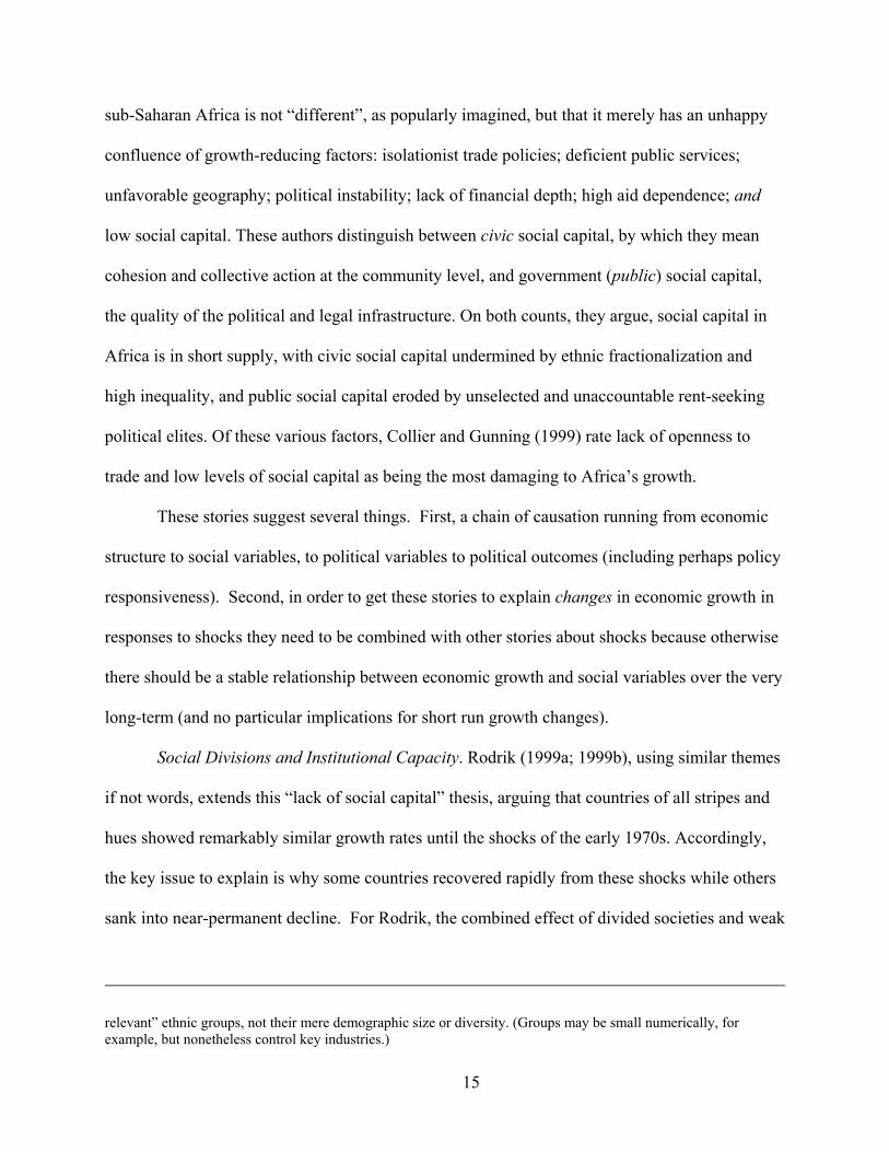
sub-Saharan Africa is not “different”, as popularly imagined, but that it merely has an unhappy

confluence of growth-reducing factors: isolationist trade policies; deficient public services;

unfavorable geography; political instability; lack of financial depth; high aid dependence; and

low social capital. These authors distinguish between civic social capital, by which they mean

cohesion and collective action at the community level, and government (public) social capital,

the quality of the political and legal infrastructure. On both counts, they argue, social capital in

Africa is in short supply, with civic social capital undermined by ethnic fractionalization and

high inequality, and public social capital eroded by unselected and unaccountable rent-seeking

political elites. Of these various factors, Collier and Gunning (1999) rate lack of openness to

trade and low levels of social capital as being the most damaging to Africa’s growth.

These stories suggest several things. First, a chain of causation running from economic

structure to social variables, to political variables to political outcomes (including perhaps policy

responsiveness). Second, in order to get these stories to explain changes in economic growth in

responses to shocks they need to be combined with other stories about shocks because otherwise

there should be a stable relationship between economic growth and social variables over the very

long-term (and no particular implications for short run growth changes).

Social Divisions and Institutional Capacity. Rodrik (1999a; 1999b), using similar themes

if not words, extends this “lack of social capital” thesis, arguing that countries of all stripes and

hues showed remarkably similar growth rates until the shocks of the early 1970s. Accordingly,

the key issue to explain is why some countries recovered rapidly from these shocks while others

sank into near-permanent decline. For Rodrik, the combined effect of divided societies and weak

relevant” ethnic groups, not their mere demographic size or diversity. (Groups may be small numerically, for example, but nonetheless control key industries.)

16

institutions of conflict management explains why the series of eternal shocks in the 1970s were

unable to be absorbed. As such, he argues that openness to trade should be a component of, not a

substitute for, a national development strategy centered on forging broad domestic social

coalitions and constructing effective institutions for managing conflict.

This approach, as we shall see, is particularly important for explaining Pritchett's (1997)

“mountains” in the evaluation of output in resource-abundant economies, which are frequently

subjected to severe, and potentially destabilizing, economic shocks (Figure 2). This does not

suggest that resource economies will have a steady state growth rate that is higher or lower, but

that the response to the shock will be less effective because of weak social capacity to respond.

In this sense, the natural resource is a double curse because (a) resource dependent economies

are more likely to experience a negative shock of substantial magnitude, and (b) resource

abundant economies are less likely to have developed socially cohesive mechanisms and

institutional capacities for accommodating the shock when it comes.

The political/social dimension of our story can therefore be summarized as follows. Some

areas of geographic space are conducive to small holder production on individually owned plots.

The interactions among these producers tend to be horizontal relationships of equality. In other

areas of geographic space production is conducive to large scale production (e.g. plantations of

bananas). In these regions the relationships tend to bind each person to a social superior (noble,

land-owner), and the horizontal relationships among producers tend to be ones of distrust. This

economic structure then produces a social structure which is conducive to “bad” politics

(clientelism) and to “bad” governance (since citizens cannot cooperate to demand better services

17

from the state).

Summary of the stories

Period of the effect Channel of

Mechanisms Long-run levels Longish-run growth

Political Moore, Putnam (Modernization effect)

Ross, Bates (Rentier effect)

Economic Engerman, Sokoloff (Entrenched inequality effect)

Sachs, Warner (Dutch disease)

Political Economy Rodrik, Easterly (Social divisions effect)

Rodrik, Pritchett (Institutional quality effect)

C. Our hypothesis

As shown above, the central thrust of most of the research on social capital and growth has been

to treat social capital as an independent variable. We argue here that it is worthwhile to look at

the effects of different types of natural resource endowments on social capital formation, since

certain types of natural resource economies appear to experience more volatile growth patterns

than others (Figure 2) – and various “social features” seems to be correlated with growth patterns

(as shown in the previous sub-section).

Our analysis builds on export base theory and the multiple consequences of different

staples for economic linkages and for social relationships. Plantation crops (cotton, sugar

processing, tobacco) as well as oil and hard minerals are typically associated with highly

concentrated ownership. This renders the state heavily dependent on a small number of owners

18

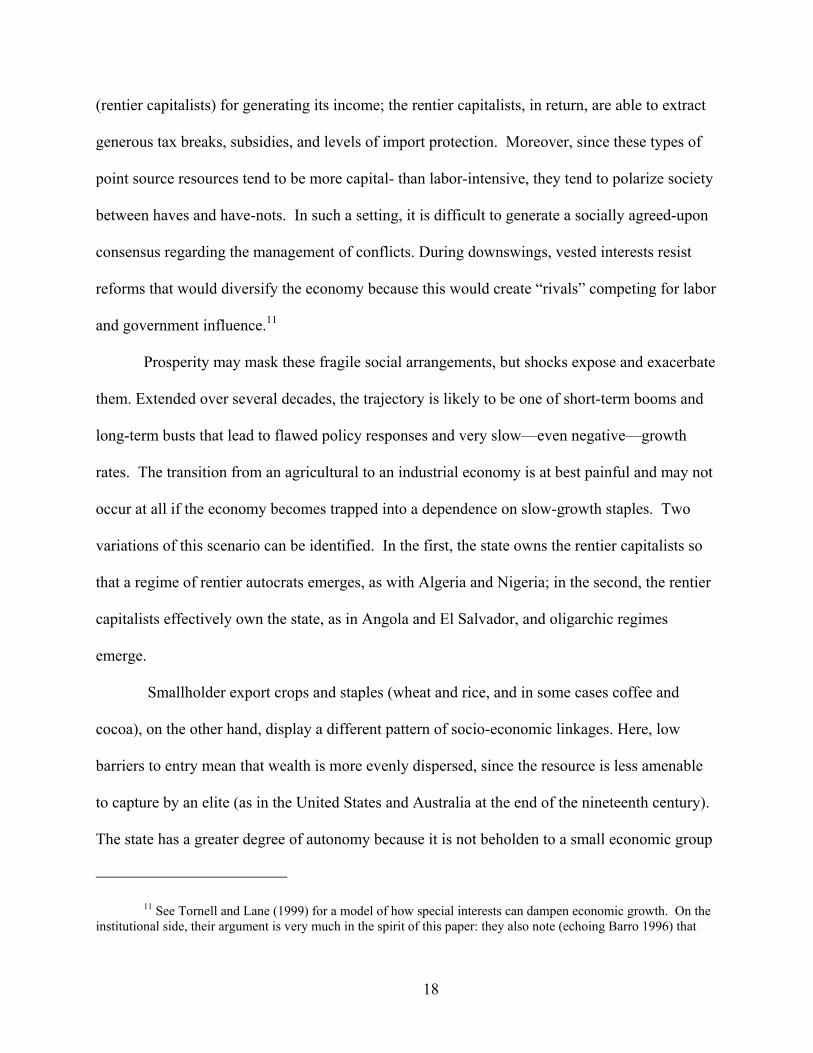
(rentier capitalists) for generating its income; the rentier capitalists, in return, are able to extract

generous tax breaks, subsidies, and levels of import protection. Moreover, since these types of

point source resources tend to be more capital- than labor-intensive, they tend to polarize society

between haves and have-nots. In such a setting, it is difficult to generate a socially agreed-upon

consensus regarding the management of conflicts. During downswings, vested interests resist

reforms that would diversify the economy because this would create “rivals” competing for labor

and government influence.11

Prosperity may mask these fragile social arrangements, but shocks expose and exacerbate

them. Extended over several decades, the trajectory is likely to be one of short-term booms and

long-term busts that lead to flawed policy responses and very slow—even negative—growth

rates. The transition from an agricultural to an industrial economy is at best painful and may not

occur at all if the economy becomes trapped into a dependence on slow-growth staples. Two

variations of this scenario can be identified. In the first, the state owns the rentier capitalists so

that a regime of rentier autocrats emerges, as with Algeria and Nigeria; in the second, the rentier

capitalists effectively own the state, as in Angola and El Salvador, and oligarchic regimes

emerge.

Smallholder export crops and staples (wheat and rice, and in some cases coffee and

cocoa), on the other hand, display a different pattern of socio-economic linkages. Here, low

barriers to entry mean that wealth is more evenly dispersed, since the resource is less amenable

to capture by an elite (as in the United States and Australia at the end of the nineteenth century).

The state has a greater degree of autonomy because it is not beholden to a small economic group

11 See Tornell and Lane (1999) for a model of how special interests can dampen economic growth. On the institutional side, their argument is very much in the spirit of this paper: they also note (echoing Barro 1996) that

19

and must instead appeal to and appease a more diverse constituency. Such a wider constituency

tends to favor the mobilization of tax revenues for investments in human capital (education and

health care) as well as for economic infrastructure. In addition the wider diffusion of wealth is

more conducive to democratic institutions so that state-society relations in smallholder

economies generate a more sophisticated social consensus regarding conflict management.

Consequently, when shocks occur, capital, labor, and the state have a broader array of social

(human and institutional) resources to call upon to help mediate the crisis. This, in turn, fosters

greater economic flexibility to adjust from slow-growth to high-growth commodities and escape

the staple trap. Extended over several decades, a trajectory of longer-term booms and shorter-

terms busts emerges, generating modest but substantial overall growth rates. Diversification into

an industrial economy, if not always smooth, nonetheless occurs, and does so more or less

evenly.

As detailed below, our approach to test this chain of causality—from natural resource

endowments to socioeconomic and political institutions to economic growth—takes a novel

methodological step by documenting that it is certain types of natural resources, not resources

per se, that cause problems.

Our hypothesis can therefore be stated as follows. Different types of natural resource

endowments matter for economic growth by generating a differential capacity to respond to

economic (and other) shocks. In particular, countries dependent on point-source natural

resources are predisposed to heightened social divisions and weakened institutional capacity,

which in turn impede their ability to respond effectively to shocks. The effective and equitable

one possible explanation for the distributive struggle in many countries is the attempt to appropriate rents generated by natural resource endowments.

20

management of shocks—and economic transitions more generally—is a key to sustaining rising

levels of prosperity.

II. Creating a measure of export structure

To test this hypothesis, we created classifications of countries, according to their natural resource

base. Using UNCTAD’s Handbook of International Trade and Development Statistics (1988),

we assembled data on the leading export staples of every country in 1985 that had a GNP per

capita under $10,000 and a population greater than one million. UNCTAD classifies export

structures into five categories: foods, agricultural raw materials, fuels, minerals, and

manufacturing. Within the leading export category, we listed the two most important

commodities, enabling us to classify countries into four types:

• ‘Non-resource abundant economies’ are comprised of ‘manufacturing’ economies, which

have, since the 1960s, relied primarily on manufacturing for their export earnings.

Resource-exporters economies’ are comprised of three sub-classifications:

• ‘Point source’ economies have relied primarily on fuels, minerals, and plantation crops

(e.g. sugar);

• ‘Diffuse’ economies have relied primarily on animals and agricultural produce grown on

small family farms (e.g., rice and wheat);

• ‘Coffee and cocoa’ have relied primarily on these two commodities (classifying them as

either ‘point source’ or ‘diffuse’ proved problematic since these crops can be grown

21

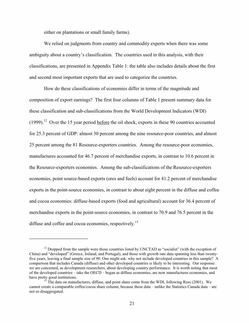
either on plantations or small family farms).

We relied on judgments from country and commodity experts when there was some

ambiguity about a country’s classification. The countries used in this analysis, with their

classifications, are presented in Appendix Table 1: the table also includes details about the first

and second most important exports that are used to categorize the countries.

How do these classifications of economies differ in terms of the magnitude and

composition of export earnings? The first four columns of Table 1 present summary data for

these classification and sub-classifications from the World Development Indicators (WDI)

(1999).12 Over the 15 year period before the oil shock, exports in these 90 countries accounted

for 25.3 percent of GDP: almost 30 percent among the nine resource-poor countries, and almost

25 percent among the 81 Resource-exporters countries. Among the resource-poor economies,

manufactures accounted for 46.7 percent of merchandise exports, in contrast to 10.6 percent in

the Resource-exporters economies. Among the sub-classifications of the Resource-exporters

economies, point source-based exports (ores and fuels) account for 41.2 percent of merchandise

exports in the point-source economies, in contrast to about eight percent in the diffuse and coffee

and cocoa economies: diffuse-based exports (food and agricultural) account for 36.4 percent of

merchandise exports in the point-source economies, in contrast to 70.9 and 76.5 percent in the

diffuse and coffee and cocoa economies, respectively.13

12 Dropped from the sample were those countries listed by UNCTAD as “socialist” (with the exception of China) and “developed” (Greece, Ireland, and Portugal), and those with growth rate data spanning less than twenty-five years, leaving a final sample size of 90. One might ask: why not include developed countries in this sample? A comparison that includes Canada (diffuse) and other developed countries is likely to be interesting. Our response: we are concerned, as development researchers, about developing country performance. It is worth noting that most of the developed countries – take the OECD – began as diffuse economies, are now manufactures economies, and have pretty good institutions.

13 The data on manufactures, diffuse, and point share come from the WDI, following Ross (2001). We cannot create a comparable coffee/cocoa share column, because these data – unlike the Statistics Canada data – are not so disaggregated.

22

Table 1: Export compositions and the natural resource base of selected developing economies Data

source World Development Indicators Statistics Canada World Trade Data Base

UNCTAD-based Classification

Exports/GDP Manufactures share

Diffuse share

Point source share

Manufactures index

Diffuse index

Point source index

Coffee and

Cocoa index

All country means

25.3 13.2 51.4 25.3 -0.33 0.05 0.04 0.06

of which: Resource-poor 29.8 46.8 33.5 7.3 -0.14 -0.04 -0.17 0.01Resource rich 24.8 10.6 52.9 26.8 -0.36 0.06 0.08 0.07 of which: Diffuse 18.9 10.6 70.9 8.1 -0.34 0.17 -0.08 0.04 Point

source 28.7 9.7 36.4 41.2 -0.35 -0.01 0.23 0.04

Coffee and cocoa

20.4 12.7 76.5 8.7 -0.39 0.10 -0.07 0.19

Notes: means of selected export and trade related data for 90 developing economies. See text for descriptions of country classifications, data and data sources.

The final four columns of Table 1 present summary data (from the Statistics Canada World

Trade Data Base) of indices that mirror our four classifications for these classification and sub-

classifications.14 As detailed in Appendix Table 2, they are created by adding net export shares

for a range of product and commodity sub-categories: for example, the ‘point source index’ is

the um of petroleum and raw materials net export shares, where raw materials include metals,

natural gas, coal, and fertilizers. While these are not available for our full set of 90 countries

(see the cautionary footnote below), they provide a useful check that our classifications are

basically valid. The ‘manufactures index’ among the resource rich countries is much lower than

14 These indices were also used in Leamer et al. (1999).

23

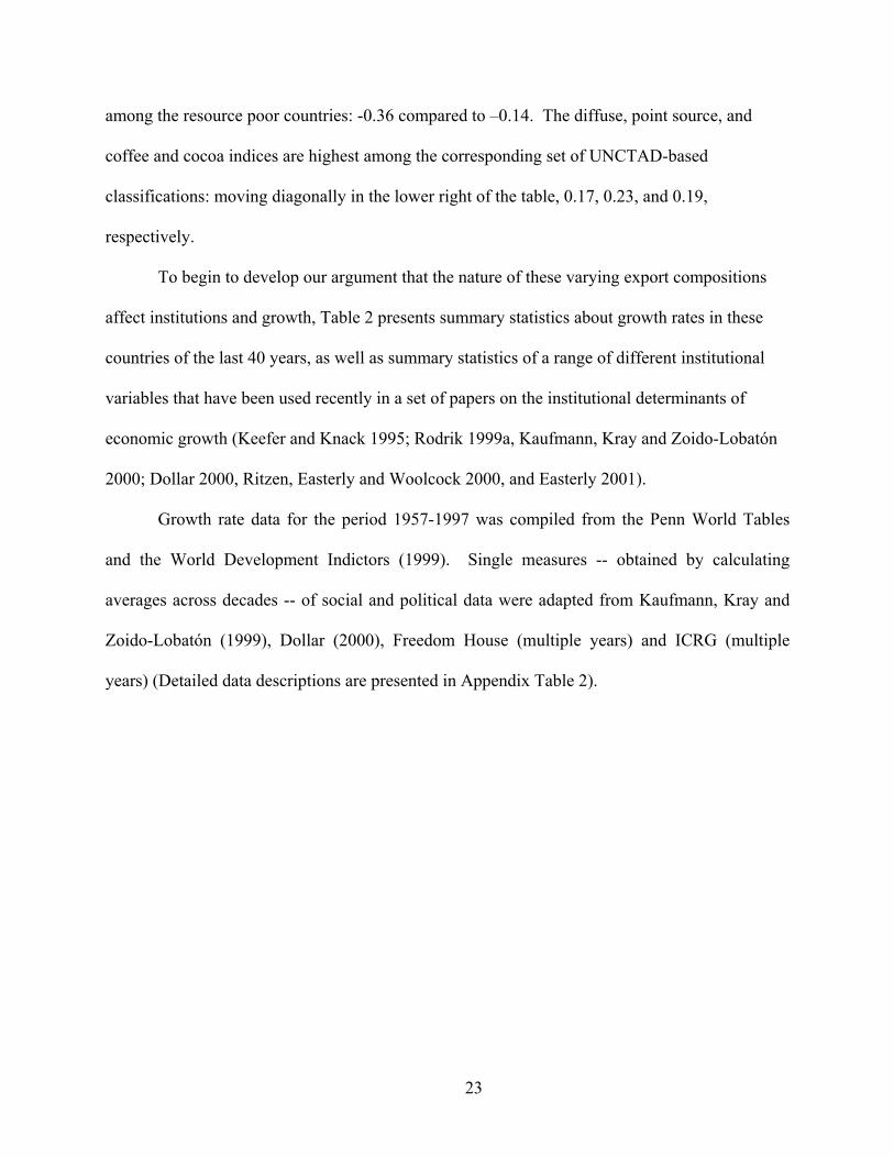
among the resource poor countries: -0.36 compared to –0.14. The diffuse, point source, and

coffee and cocoa indices are highest among the corresponding set of UNCTAD-based

classifications: moving diagonally in the lower right of the table, 0.17, 0.23, and 0.19,

respectively.

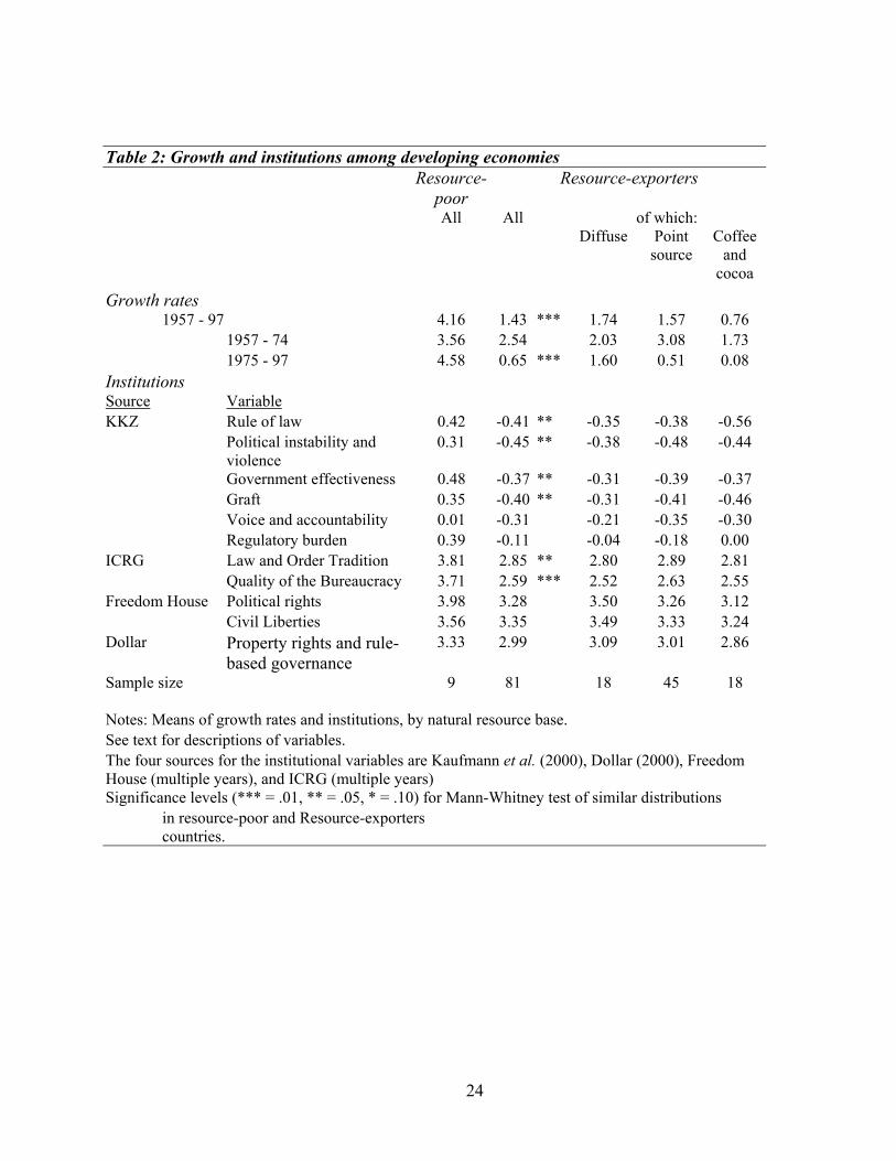
To begin to develop our argument that the nature of these varying export compositions

affect institutions and growth, Table 2 presents summary statistics about growth rates in these

countries of the last 40 years, as well as summary statistics of a range of different institutional

variables that have been used recently in a set of papers on the institutional determinants of

economic growth (Keefer and Knack 1995; Rodrik 1999a, Kaufmann, Kray and Zoido-Lobatón

2000; Dollar 2000, Ritzen, Easterly and Woolcock 2000, and Easterly 2001).

Growth rate data for the period 1957-1997 was compiled from the Penn World Tables

and the World Development Indictors (1999). Single measures -- obtained by calculating

averages across decades -- of social and political data were adapted from Kaufmann, Kray and

Zoido-Lobatón (1999), Dollar (2000), Freedom House (multiple years) and ICRG (multiple

years) (Detailed data descriptions are presented in Appendix Table 2).

24

Table 2: Growth and institutions among developing economies Resource-

poor Resource-exporters

All All of which: Diffuse Point

source Coffee

and cocoa

Growth rates 1957 - 97 4.16 1.43 *** 1.74 1.57 0.76 1957 - 74 3.56 2.54 2.03 3.08 1.73 1975 - 97 4.58 0.65 *** 1.60 0.51 0.08

Institutions Source Variable KKZ Rule of law 0.42 -0.41 ** -0.35 -0.38 -0.56

Political instability and violence

0.31 -0.45 ** -0.38 -0.48 -0.44

Government effectiveness 0.48 -0.37 ** -0.31 -0.39 -0.37 Graft 0.35 -0.40 ** -0.31 -0.41 -0.46 Voice and accountability 0.01 -0.31 -0.21 -0.35 -0.30 Regulatory burden 0.39 -0.11 -0.04 -0.18 0.00

ICRG Law and Order Tradition 3.81 2.85 ** 2.80 2.89 2.81 Quality of the Bureaucracy 3.71 2.59 *** 2.52 2.63 2.55

Freedom House Political rights 3.98 3.28 3.50 3.26 3.12 Civil Liberties 3.56 3.35 3.49 3.33 3.24

Dollar Property rights and rule-based governance

3.33 2.99 3.09 3.01 2.86

Sample size 9 81 18 45 18

Notes: Means of growth rates and institutions, by natural resource base. See text for descriptions of variables. The four sources for the institutional variables are Kaufmann et al. (2000), Dollar (2000), Freedom House (multiple years), and ICRG (multiple years) Significance levels (*** = .01, ** = .05, * = .10) for Mann-Whitney test of similar distributions

in resource-poor and Resource-exporters countries.

25

First, this table shows the growth story that we introduced with Figures 1 and 2: since the

oil shock, annual growth rates of GDP per capita have been significantly (using the non-

parametric Mann - Whitney test) different between the resource poor and resource rich countries:

4.58 and 0.65, respectively. Likewise, growth rates among the Resource-exporters

classifications – 1.60, 0.51, and 0.08, respectively – are also significantly (using Mann –

Whitney again) different: diffuse economies have done almost as well as their pre-oil shock

performance; point source and coffee/cocoa economies have floundered. Second, the case of all

eleven institutional variables, the mean is lower (institutionally worse, in all cases) among the

Resource-exporters countries: in the case of six of these, this difference is statistically

significant: from the KKZ data, ‘rule of law’, ‘political instability’, ‘government effectiveness’,

and ‘graft’; from ICRG, ‘law and order tradition’ and ‘quality of the bureaucracy.’ Third, in the

case of the nine institutional variables—the exceptions are ‘law and order tradition’ and ‘quality

of the bureaucracy’—the mean is higher among the diffuse economies compared to point source

and coffee/cocoa economies (though in no case is this difference statistically significant). As

exemplified by the extreme case of Angola, Resource-exporters countries—particularly those

with a point source or coffee/cocoa natural resource base—are more likely to have low economic

growth and weak socioeconomic and political institutions.

Building on the anecdotes, arguments, and cross tabulations presented in this section, we

econometrically test in the next sections whether (a) countries that are abundant (scarce) in

point-source natural resources have weaker (stronger) institutional capacities; and (b) these

endogenously determined institutional capacities are significant and large determinants of growth

26

since the oil shock.

III: The econometric model and the data

As discussed and established in many previous studies of the institutional determinants of

growth, instrumental variables and three stage least square (3SLS) estimation are improvements

on OLS estimation, since the former corrects for the likelihood of omitted variable and

simultaneity bias. Making these corrections is critical for the exercise in this paper. Despite the

machinations that we report in the robustness test below, it would be shocking if there weren’t

some omitted variable that affected growth among these countries in this period and that is

correlated with our institutional variables of interest. This omission, of course, could lead to a

biased estimate of the effect of the institutions. Likewise, it seems obvious that economic

growth, to some degree, will effect – through time – a country’s socioeconomic and political

institutions. The challenge of an exercise like ours is, of course, to find an appropriate

instrument: correlated with the regressor of interest and uncorrelated with the error term of the

regression of interest. More colloquially, it has to be ‘truly’ exogenous.

Previously, researchers have used shares of English and European language speakers

(Hall and Jones 1999; Kaufmann et al. 2000) and ethnic fractionalization (Ritzen, Easterly, and

Woolcock 2000) as such instruments in growth regressions15. Our basic strategy in this section

is to show that the addition of natural resource base variables to an instrument set that also

15 There is a critical difference between the first two -- Hall and Jones (1999) and Kaufmann et al. (2000) – and ‘Barro’ growth regression papers like Ritzen, Easterly, and Woolcock (2000), the Sachs and Warner set, and this paper: the former use the log of levels of per capita income and output, respectively, as dependent variables; the latter use growth rates of per capita income as the dependent variable. We believe that specifications like those in Hall and Jones (1999) and Kaufmann et al. (2000) are in many ways the best way to look at changes in well being (qua income). We adopt the ‘Barro’ specifications in this paper because we are explicitly trying to explain the collapse of growth rates among point source and coffee/cocoa economies, as illustrated by Figure 2.

27

includes these variables improves the 3SLS estimation16 of the institutional determinants of

growth among 90 developing countries since the oil shock. Specifically, we show that such IV

estimates lower the standard error for these estimates and increase—in some cases by a lot—the

point estimate for the effect of the institution.

To do so, we first use an econometric model which builds on the system of equations

frameworks in Kaufmann et al. (2000) and Ritzen et al. (2000), in which intuitional variables are

endogenously determined. Our econometric analysis differs from those and others as follows:

we use a full set of other RHS variables that are know to be associated with growth (unlike

Kaufmann et al. 2000); and – as noted above -- we use variables associated with the natural

resource base as instruments. Specifically, we add two alternative natural resource base

variables—from Woolcock, Pritchett and Isham (2001) and Leamer et al. (1999)—to an

instrument set that includes Hall and Jones language variables (as in Kaufmann et al. 2000) and

ethnic fractionalization (as in Ritzen, Easterly, and Woolcock 2000)

Our model for the determinants of the growth of GDP per capita from 1975 to 1997 in

country i (‘growthi’) is:

(1) Iij = β0 + β1*NRi + β2*Wi + β3* Xi + εi

(2) Growthi = α0 + α1* Iij + α2*Xi + ηi

j = 1 … 6

where

• Ii is an endogenously-determined institutional variable;

• NRi is a vector of exogenously-determined ‘natural resource base’ variables;

16 This seems to be the estimation technique of choice among the growth cognoscenti. 3SLS estimates are more efficient than IV estimates if the error terms below are correlated.

28

• Wi is a vector of other exogenously-determined variables;

• Xi is a vector of previously-identified determinants of growth,

• εi and ηi are error terms with the usual properties.

The data that are used to test his model are listed below. (Detailed data descriptions and

sources are presented in Appendix Table 2).

• The six institutional variables (Ii) are ‘rule of law’, ‘law and order tradition’, ‘political

instability’, ‘government effectiveness’, ‘graft’ and ‘quality of the bureaucracy.’ As a

reminder, these were the six institutional variables that were significantly different

between Resource-exporters and resource-poor economies in Table 2.

• The two natural resource base instruments (NRi) are: dummies for the UNCTAD

classifications (’diffuse’, ’point source’ and ‘coffee and cocoa’) and; indices from the

Statistics Canada classifications (again, ’diffuse’, ’point source’ and ‘coffee and cocoa’).

• The other instruments (Wi) are ‘English language’, ‘European language’, ‘Distance from

equator’, and ‘Predicted trade share’ (used in Hall and Jones 1999) and ‘ethnolinguistic

fractionalization’ (used in Ritzen, Easterly, and Woolcock 2000)

• Previously-identified determinants of growth (Xi): ‘natural resource share of GDP

(1974)’; ‘per Capita GDP (1975)’; ‘investment price level (1975)’; ‘secondary school

achievement (1960)’; ‘trade openness’; and regional dummies for sub-Saharan Africa,

Europe and the Middle East, Latin America, and East Asia.17

17 For a robustness check of adding other independent variables from highlighted in Barro (1991), Levine and Renelt (1992), and Sala-i-Martin (1997), among others, see the next section.

29

• The growth rate of per capita GDP (growthi) is the mean of this growth rate from 1975 –

1997 (World Bank 1999).

Among the Xi variables, there is one regressor above all that is critical to include and

draw attention to: ‘natural resource share of GDP (1974).’ This is the measure that is used to

test the ‘natural resource curse’ in Sachs and Warner (beginning with 1995). By including it as a

regressor, where indicators of the natural resource-base composition of exports are used as

instruments for institutions, we can also the following hypothesis: that the ‘natural resource

curse’ can be partially explained by our endogenously determined instruments. This would

result in a lower coefficient -- compared to an OLS model -- on ‘natural resource share of GDP

(1974)’ when equations 1 and 2 are estimated simultaneously. We can also test the hypothesis --

using statistical tests from Hausman (..), Hausman and Taylor (..), and Davidson and MacKinnon

(1993) -- whether these instruments, like ‘natural resource share of GDP (1974),’ actually

belong in the estimation of the structural equation or are otherwise poorly chosen.

IV: The results

First, we present the results for estimating equation (1). This establishes whether measures of the

natural resource endowment predict the nature of socioeconomic and political institutions)

(specifically, whether we can reject the null that β1 = 0 holds in the estimation of equation 1).

Table 3 illustrates an OLS test of equation (1) for ‘rule of law,’18 where we first add each

of the NRi variables to a model which includes the Xi variables -- specifications (1) through (3) --

18 The other five institutional variables produce basically similar results to those reported here.

30

and then add each of the NRi variables to a model which includes the both Xi and Wi variables --

specifications (4) through (6).19 These results show that the UNCTAD categories -- ‘diffuse’,

‘point source’, and ‘coffee and cocoa’ -- do help to predict ‘government effectiveness’ more or

less as we would have expected. ‘Point source’ is statistically significant at the 0.10 level or

below in specifications 2 and 5; ‘coffee and cocoa’ is only in specification 5 (remember for later:

this is a test whether each of the categories is statistically different from ‘resource poor’, the

omitted category). The ‘point source’ category has the lowest point estimate (-0.53 in

specification 2; -0.82 in specification 5), and ‘diffuse’ has the highest point estimate (-0.28 in

specification 2; -0.49 in specification 5). We cannot reject the null that the entire vector β1 = 0

(the p-values for such f-tests are 0.300 and 0.208). Overall, these results suggest that ‘point

source’ is the critical natural resource determinant of ‘rule of law’. 20

The mostly similar pattern is found with the Statistics Canada indices. The point source

index is statistically significant (in this case, not in comparison to an omitted variable21) in both

specifications. In specification 5, the other two indices, not statistically significant, do have the

expected signs and relative (to the point source index) magnitudes. There is one ‘surprising’

result, in specification 2, ‘diffuse’ is significant, and its point estimate, while lower than ‘point

source’, is slightly higher than ‘coffee and ‘cocoa.’ Since we use the full set of W’s to estimate

(1), allow us not to make too much of this result. Finally, in this case, we can easily reject the

null that β1 = 0.

19 The savvy reader might ask why we are not presenting the results from 3SLS versions of the variants of equation (1). Frankly, it is much easier to create this table, when using STATA, with OLS results! An inspection of these results and those of the 3SLS version reveal only very slight differences. See the footnote below on the 3SLS results for all six variables that are comparable to those of specification 6 in Table 3.

20 A small note about the scale and definition of ‘Per capita GDP (1975)’ in this table: it is in US$1000, adjusted for purchasing power parity.

31

21 Why not use all four Statistics Canada indices here? When they all are used in the test of equation 2 (as detailed below), the system is overidentified. This is not true when only these three are used. The reasons for this will be clarified in due time.

32

Table 3: The effect of the natural resource base on rule of lawSp ecification

Indep endent variablesPer Cap ita GDP (1975) 0.084 * 0.076 * 0.110 *** 0.060 0.042 0.092 **

(0.044) (0.045) (0.040) (0.045) (0.046) (0.042)Investment p rice (1975) -0.086 -0.077 -0.054 -0.076 -0.086 -0.050

(0.091) (0.091) (0.084) (0.087) (0.086) (0.081)Secondary school (1960) 0.029 ** 0.029 ** 0.028 ** 0.019 0.017 0.020 *

(0.012) (0.012) (0.011) (0.012) (0.012) (0.011)Trade op enness 0.98 *** 0.85 *** 0.92 *** 0.97 *** 0.82 *** 0.94 ***

(0.31) (0.31) (0.28) (0.30) (0.31) (0.27)Latitude 0.00003 0.00005 0.00010 ** -0.00001 0.00000 0.00007

(0.0000) (0.0000) (0.0000) (0.0001) (0.0001) (0.0001)Sub-Saharan Africa 0.16 0.43 0.57 * -0.13 0.22 0.41

(0.29) (0.33) (0.29) (0.34) (0.37) (0.34)Europ e / M iddle East 0.61 * 0.91 ** 0.93 *** 0.60 1.16 ** 1.12 ***

(0.35) (0.38) (0.32) (0.38) (0.46) (0.37)Latin America -0.06 0.26 0.35 -0.84 ** -0.45 -0.20

(0.29) (0.35) (0.30) (0.42) (0.46) (0.43)East Asia 0.16 0.33 0.33 0.22 0.35 0.47

(0.37) (0.38) (0.33) (0.38) (0.38) (0.35)

English language -0.14 0.02 -0.04(0.41) (0.42) (0.38)

Europ ean language 0.88 ** 0.91 ** 0.74 *(0.41) (0.41) (0.39)

Latitude -0.0074 -0.0096 * -0.0049(0.0052) (0.0053) (0.0048)

Predicted trade share 0.32 ** 0.25 * 0.11(0.14) (0.14) (0.14)

Ethnic fractionalization -0.0007 0.0003 0.0018(0.0029) (0.0030) (0.0027)

Diffuse (UNCTAD) -0.28 -0.49

(0.30) (0.38)Point source (UNCTAD) -0.53 * -0.82 *

(0.30) (0.42)Coffee and cocoa (UNCTAD) -0.44 -0.75 *

(0.35) (0.43)Diffuse (Stats Canada) -0.9279 * -0.5473

(0.5276) (0.6010)Point source (Stats Canada) -1.2538 *** -1.2873 ***

(0.3025) (0.3519)Cofee and Cocoa (Stats Canada) -0.8292 -1.0045

(0.6727) (0.6689)Adjusted r-squared 0.500 0.506 0.598 0.545 0.559 0.631

Sample size 74 74 74 69 69 69F - test for new variable set (p-values) -- 0.300 0.000 0.054 0.208 0.0034

Notes: test of the effect of two different sets of natural resouce base indicators on rule of lawSee test for descrip tions of all variables. Significance levels are: *** = .01, ** = .05, * = .10

Natural resource instruments

(5) (6)

'Determinants of growth'

'Other instruments'

(1) (2) (3) (4)

33

What are the magnitudes of these effects? From specification 5, a country that (rather

magically) went from being in the point source classification to the resource-poor classification

would increase ‘rule of law’ by 0.82; from specification 6, a country whose point source index

fell by two standard deviations (=0.30*2) – as equally magical a change -- would increase ‘rule

of law’ by 0.77. Since the standard deviation of ‘rule of law’ is 0.78, these represent substantial

institutional improvements. The same holds (not shown; we can show you) with the other five

institutional variables of interest. In fact, the coefficients of ‘point source’ in the first stage of

the 3SLS estimates of the complete system imply that the effect of this magical change is at least

slightly greater than the standard deviation of the corresponding institutions variable. ‘Rule of

law’, it turns out, has the lowest comparable effect; ‘government effectiveness’, the highest,

corresponds to a two standard deviation change!22

So the results summarized above are what we had hoped for. Controlling for our X’s and

W’s, two different sets of natural resource variables are significant and large determinants of

socioeconomic and political institutions.

Next, we present the results of estimating equation (2) with the UNCTAD instruments

and the Statistics Canada instruments, respectively. A word about the organization of Tables 4

and 5: each cell in the row with the variable name is a coefficient from an OLS or 3SLS estimate,

as noted. The cell below that is the standard error, and the cell below that is the sample size.

22 Using the first – stage results from specification (6) in Table 4 below, the ratios of the absolute values of the coefficients to the standard deviation are (respectively, for the six variables as listed in Table 4): 1.06; 1.35; 1.25; 2.08; 2.11 and 1.43.

34

(Appendix Table 3 will show, as an example, the full results from these OLS and IV

specifications for ‘government effectiveness’.)23

23 An important word about the results reported below in Table 5 for this ‘zero draft’. We don’t yet have the full set of available data for these natural resource indices based on the Statistics Canada trade data [GWEN, LET’S TALK!]. Thus, for about 30 of the countries used in the samples in Table 5 (which range from 68 to 77), estimated natural resource indices are used. These estimated indices are generated with stepwise regression models, where the potential determinants include the WDI export shares reported in Table 1 (for a range of years ), regional dummies, and the UNCTAD dummies. The reader is invited to insert his/her violent objection to this technique here: ____________. Happily, we can report that VERY similar coefficients -- with (as one would expect) larger standard errors – can be generated by using smaller samples (about 45 or so) with only the actual indices.

35

Table 4: The institutional determinants of growth, accounting for the natural resource endowment: UNCTAD variables as the natural resource instrument

Estimation procedure OLS 3SLS 3SLS 3SLS 3SLS 3SLSInstruments - Partial W Natural

resourcesPartial W and natural resources

Full W Full W and natural resources

Rule of law 1.19 *** 1.63 2.09 * 1.82 *** 1.18 1.48 **(0.33) (1.11) (1.07) (0.71) (0.73) (0.62)

69 69 69 69 69 69

Law and order 0.63 * 1.72 2.26 * 1.91 *** 1.39 ** 1.55 **(0.32) (1.29) (1.37) (0.73) (0.65) (0.61)

60 60 60 60 60 60

Political instability 0.49 1.51 2.41 * 2.20 ** 1.17 1.56 **(0.32) (1.30) (1.45) (0.94) (0.80) (0.72)

65 65 65 65 65 65

Government effectiveness 0.72 ** 1.74 2.01 * 2.04 *** 0.77 1.23 **(0.36) (1.36) (1.07) (0.78) (0.85) (0.61)

66 66 66 66 66 66

Graft 1.06 ** 2.24 2.42 ** 2.21 *** 1.75 * 1.86 ***(0.42) (1.57) (1.23) (0.77) (0.93) (0.69)

65 65 65 65 65 65

Quality of bureacracy 0.15 1.19 0.14 0.81 1.28 0.76(0.29) (0.90) (0.71) (0.51) (0.89) (0.50)

60 60 60 60 60 60

Note: the coefficients, standard errors, and sample sizes from six multivariate regressions for each of six institutional variables. The dependent variable is per capita growth from 1974 - 1997. The results from other covariates in the model are not reported here. Partial W instruments are the languages variables and 'latitude'; Full W 's add 'ethnic fractionalization' and 'predicted trade share.'Significance levels are: *** = .01; ** = .05; * = .10. See the text for descriptions of the variables and the econometric specifications.

36

Table 5: The institutional determinants of growth, accounting for the natural resource endowment: Statistics Canada variables as the natural resource instrument

Estimation procedure OLS 3SLS 3SLS 3SLS 3SLS 3SLSInstruments - Partial W Natural

resourcesPartial W and natural resources

Full W Full W and natural resources

Rule of law 1.19 *** 1.63 1.05 * 1.09 ** 1.18 0.99 **(0.33) (1.11) (0.56) (0.51) (0.73) (0.50)

69 69 69 69 69 69

Law and order 0.63 * 1.72 0.84 1.10 * 1.39 ** 1.16 **(0.32) (1.29) (0.69) (0.62) (0.65) (0.57)

60 60 60 60 60 60

Political instability 0.49 1.51 1.13 * 1.12 * 1.17 0.93 *(0.32) (1.30) (0.65) (0.59) (0.80) (0.55)

65 65 65 65 65 65

Government effectiveness 0.72 ** 1.74 1.34 * 1.32 * 0.77 0.69(0.36) (1.36) (0.79) (0.69) (0.85) (0.59)

66 66 66 66 66 66

Graft 1.06 ** 2.24 1.38 * 1.51 ** 1.75 * 1.39 **(0.42) (1.57) (0.77) (0.69) (0.93) (0.68)

65 65 65 65 65 65

Quality of bureacracy 0.15 1.19 1.37 * 1.37 ** 1.28 0.93 *(0.29) (0.90) (0.81) (0.62) (0.89) (0.51)

60 60 60 60 60 60

Note: the coefficients, standard errors ,and sample sizes from six multivariate regressions for each of six institutional variables. The dependent variable is per capita growth from 1974 - 1997. The results from other covariates in the model are not reported here. Partial W instruments are the languages variables and 'latitude'; Full W 's add 'ethnic fractionalization' and 'predicted trade share.'Significance levels are: *** = .01; ** = .05; * = .10. See the text for descriptions of the variables and the econometric specifications.

37

The results in Tables 4 and 5 can be summarized as follows. First, when the

languages variables and ‘latitude’ are used as instruments for each of the six institutional

variables -- labeled ‘Partial W’ in the tables -- the resulting coefficient (specification 2) is

usually not significant (although a Hausman test that the efficient estimate (OLS -

specification 1) and the consistent estimate (3SLS – specification 2) are equal cannot be

rejected). Put another way, the language variables and ‘latitude’, on their own, are not

good enough predictors of the institutions variables – and thus cannot solve the OMV and

simultaneity problems that are likely present in the OLS models (specification 1).

By contrast, when the UNCTAD variables (Table 4) or the Statistics Canada

variables (Table 5) are the only the instrument set (specification 3), this usually generates

an estimate that is greater than the OLS estimate and is significant. The exceptions are

‘quality of the bureaucracy’ in table 4 and ‘law and order’ in Table 5.

When the languages variables and ‘latitude’ are added to the natural resource

variables (specification 4), things get even better: in nine of the previous 12 cases, this

lowers the standard error enough to notably increase the significance of this larger

(compared to OLS) estimate.24

One might say that these results so far tell us little: maybe there are plenty of

alternative instruments – including trade-related ones -- that could do this. Well,

specification 5 shows that if you add ‘ethnic fractionalization’ and ‘predicted trade share’

to the languages variables and ‘latitude’, the estimates become significant in only two

cases in each table (remember, the relevant comparison here is with specification 2). But

24 Notably?: by this we mean from the 0.10 level to the 0.01 level in most cases in Table 4, and from the 0.10 level to the 0.05 level in most cases in Table 5. Given the measurement error that is present

38

when the natural resource variables are added to these -- that is, when the full instrument

set of W’s and NR’s are used -- the estimate is significant in five cases of six cases in

each table (and again, usually quite larger than the OLS estimates).25

In just about all cases (not reported in these tables) germane statistical tests come

though fine (following the empirical strategy of Summers and Pritchett (1994)): Hausman

tests of equality of the OLS and IV coefficients: Hausman-Taylor tests of the exogeneity

of the other instruments (in this case, all instruments compared to languages and

‘latitude’); and tests for the over-identification of the system of equations.26 Overall,

what do these tests tell us: that our instrument sets are ‘exogenous’ -- no instrument,

including the natural resource base variables, seems to belong in the structural equation --

and that we have not used too many instruments to generate these results.

Now, remember the question posed above: will the inclusion of these

endogenously generated instruments in a system of equations lessen the influence of

‘natural resource share of GDP (1974)’? The answer is no. The coefficient on this

proposed measure of the ‘natural resource curse’ does not change significantly from

specification 1 – the OLS estimate – to the other specifications. (See – soon -- the

illustrative example in Appendix Table 3). So to some degree, we are still left with a

because of the construction of missing Statistics Canada data (see the previous cautionary footnote), we speculate that the pattern in Table 5 will improve when these data are fully updated.

25 In the cases of ‘government effectiveness’ and ‘ property rights in Table 5, the addition of the Statistics Canada variables lowers the relevant p-values – that is, comparing specifications 5 and 6 – from 0.26 to 0.19 and from 0.17 to 0.15.

26 And, as illustrated in Table 4, the ‘incremental r-squareds’ of the first stage regression (see the example in the appendix) show that the NR variables ‘improve’ the estimation of the institutional variables (Shea 1997).

39

mystery: why does this variable still significantly affect growth, even when the effect of

the composition of exports on institutions is accounted for?27

The results in this section comprise the econometric punch line of this paper.

Much often than not, using either of two measures of natural resource endowment as

exogenously determined instruments increases the statistical significance of the estimate

of an institution’s effect on growth, and the point estimate is usually a lot higher.

What are the implications of this higher estimate? In the first part of this section,

we noted that a large change in the composition of a country’s natural resource

endowment – a magical shift away from point source dependence – is associated with an

improvement of one standard deviation (or more) of the institutions variables. How

might such a improvement translate, based on our econometric model, translate into a

change of economic growth?

27 One potential answer is that this measure captures the affect of being in an earlier period of an economic ‘take off’ (or, if you prefer, before the realization of a ‘threshold effect’). A developing country that has not yet industrialized is likely to produce a higher share of primary products compared to one that has. If the rapidity of this industrialization path is determined by other influences besides those in this system of equations, this coefficient could persist because of OMV bias. We admit that it’s hard to point to what influences these might be, particularly given the seemingly exhaustive tests of Sachs and Warner (1995 and subsequent years) to drive out this result.

40

Table 6: The implications of the estimated effects of institutions on economic growth Magnitude of change of growth rate:

with OLS estimates

with IV estimates

difference (IV - OLS)

Rule of law 0.93 1.15 0.23 Law and order 0.60 1.47 0.87 Political instability 0.41 1.29 0.89 Government effectiveness 0.52 0.89 0.37 Graft 0.66 1.15 0.50 Quality of bureaucracy 0.15 0.75 0.60 Note: incremental changes of per capita growth rates based on standard deviation changes of institutional variables. See the text for details of these calculations.

Using the results from the UNCTAD variables in Table 4, Table 6 presents the

product of the standard deviation of each institutional variables and: the OLS coefficient

(specification 1); the full IV coefficient (specification 2)); the difference between the

OLS and the full IV coefficient (specification 3). Measured this way, using the full set of

instruments dramatically increases the magnitude of the effect of institutions on the

standard of living. To illustrate, take the median of these figures from specification 2

(1.15): this translates into a GPD per capita that, ceteris paribus, is almost 33 percent

higher, 25 years after the oil shock, among countries with better institutions (measured by

one standard deviation change) than countries with worse institutions. (The equivalent

41

calculation for the OLS estimate is 15 percent.) The large magnitude of this figure – and

the overall statistical evidence reported in this section – is consistent with our hypothesis:

that the dependence on point source endowments in selected developing countries has

dramatically lowered the standard of living via socioeconomic institutions that affect

growth.

V: Potential weaknesses of the results

What are the weaknesses of these empirical results – and how do we address these

weaknesses? Put another way, where are ‘the bodies buried’? (Pritchett, personal phrase)

For this draft, we just summarize what we’ve done with an annotated list.

1. Why not other estimation technique? (SAME RESULTS WITH 2SLS)

2. Does this story work with the other institutional variables in Table 2? (NO)

3. Does this hold up with other X variables – including the reader’s favorite? (YES, SO

FAR. WILL TRY SOME OTHER SUSPECTS, INCLUDING MANZANO AND

RIGOBON’S ‘DEBT OVERHANG’ (2001), WHICH SEEMS TO RAISE

INTERESTING ISSUES FOR THE RESULTS IN THIS PAPER AND THOSE OF

SACHS AND WARNER.)

4. What if some other quality of the relatively small number (nine) of ‘resource poor’

countries is driving these results? For example, the East Asian NICs, which are

notorious drivers of a whole range of (sometimes specious) growth results. WE GET

42

SIMILAR RESULTS, IN JUST ABOUT ALL CASES, IF WE ELIMINATE SOUTH

KOREA, HONG KONG, SINGAPORE AND TAIWAN FROM THE SAMPLE

(WITH, AS ONE WOULD EXPECT, SOMEWHAT LOWER COEFFICIENTS).

AND NB: BECAUSE OF DATA LACUNAE, CHINA IS NOT IN THE

ECONOMETRIC SAMPLE.

5. The UNCTAD variables have weaknesses as NR instruments. First, they are

dummies – and much of the predictive power comes from the ‘resource

rich’/’resource poor’ distinction as opposed to the ‘point source’, ’diffuse’,

‘coffee/cocoa’ distinction. (Remember: in the first stage regressions, we could reject

the null that the ‘point source’ countries are statistically different from ‘resource

poor’; by inspection, we can not reject the null that ‘point source’, ’diffuse’ and

‘coffee/cocoa’ are statistically different from each other). THE STORY IS NOT AS

STRONG – AGAIN, NOT SURPRISING – BUT IT MOSTLY HOLDS.

6. Another worry (still with the UNCTAD variables): does the distinction among the

resource rich countries make any difference (after all, we played it up a lot in the bulk

of the first part of the paper!). What happens if you eliminate all of the ’resource

poor’ countries from the samples, and then explicitly test the ‘point source’, ’diffuse’,

‘coffee/cocoa’ distinction? THE STORY AGAIN IS NOT AS STRONG – AGAIN,

NOT SURPRISING – BUT IT ALSO MOSTLY HOLDS: IN A NUMBER OF

CASES, THE COEFFICIENT IN SPECIFICATION 3 IS NO LONGER

SIGNIFICANT, WHILE THE REST OF THE PATTERN HOLDS.

43

VI: Discussion and conclusion

At first glance, ours are stultifying results for the policy maker: like Putnam’s (1993)

medieval guilds and choral societies, it is hard to imagine how a World Banker can

change our underlying cause of poor performance – a country’s natural resource

endowment. We admit: it is hard to get beyond this first glance.

But here’s why we think it is important to shed light on these results. Dollar and

Pritchett (1999) illustrate the power of institutions, and what donors should (and most

important, should not) do in the face of varied institutional performance among potential

aid recipients. Our results suggest how entrenched – and ‘environmentally determined’ –

that poor institutions can be (cf. Wade [1988], at micro level). So these results, in a

certain sense, further raise cautions about casual attempts at institutional reform. Poor

institutions are deeply rooted.

So what can be done? Contrast Chad (‘institutional’ conditionality from the

World Bank on their oil loan, which looks disastrous so far: money is going, defiantly, to

the purchasing of arms) to Qatar story in the New Yorker (Weaver 2000). In the latter

case, the head of state, recognizes that the natural resource gravy train – including the

institutions that have gone with it – is leaving the station. What is he trying to lead?:

reform from within. He has decreed (!) that Qatar will become a democracy: censorship

is out, universal suffrage and elections are in.

We are hopeful that in some cases, donors can – if they’re lucky – gently nudge

44

along such reforms. At very least, donors should not maintain (perceived) ‘lifeline’ aid

that prevents the likelihood of nascent reforms from even getting started.

45

References

Acemoglu, Daron, Simon Johnson, and James Robinson (2001) ‘The colonial origins of comparative development: an empirical investigation’ American Economic Review 91(5): 1369-1401

Adelman, Irma and Cynthia Taft Morris (1967) Society, Politics and Economic Development Baltimore: Johns Hopkins University Press

Aron, Janine (1997) ‘Political, economic and social institutions: a review of the growth evidence’ University of Oxford, Centre for the Study of African Economies: Working Paper Series, 98-4

Auty, Richard (1995) Patterns of Development: Resources, Policy and Economic Growth London: Edward Arnold.

Auty, Richard (2001) ‘Introduction and overview’, in R.M. Auty (ed.) Resource Abundance and Economic Development New York: Oxford University Press

Baldwin, Robert (1956) ‘Patterns of development in newly settled regions’ Manchester School of Economic and Social Studies 24: 161-179

Barro, Robert (1997) Determinants of Economic Growth: A Cross-Country Empirical Study Cambridge, MA: MIT Press

Bates, Robert (2000) Prosperity and Violence: The Political Economy of Development New York: Norton

Collier, Paul (1999a) ‘The economic causes of civil war’ Oxford Economic Papers and Bulletin

Collier, Paul (1999b) ‘The political economy of ethnicity’ Annual Bank Conference on Development Economics 1998 Washington, DC: The World Bank

Collier, Paul and Anke Hoeffler (2001) ‘Greed and grievance in civil war’ Mimeo, The World Bank (Draft: October 21)

Collier, Paul and Jan Willem Gunning (1999) ‘Explaining African economic performance’ Journal of Economic Literature 37(March): 64-111

Deininger, Klaus (1999) ‘A new data set for measuring land inequality’ The World Bank, mimeo

Diamond, Jarred (1998) Guns, Germs, and Steel: The Fates of Human Societies New York: Norton

Easterly, William (1999) ‘Life during growth” Journal of Economic Growth

Easterly, William (2000) ‘The middle class consensus and economic development’

46

Policy Research Working Paper No. 2346. Washington, DC: The World Bank

Easterly, William (2001) ‘Evidence from commodity endowments that inequality does lower per capita income’ Mimeo, The World Bank

Easterly, William and Ross Levine (1997) ‘Africa’s growth tragedy: policies and ethnic divisions’ Quarterly Journal of Economics 62(November): 1203-50

Engermann, Stanley and Kenneth Sokoloff (1997) ‘Factor endowments, institutions, and differential paths of growth among new world economies: a view from economic historians of the United States,” in Stephen Haber, ed. How Latin America Fell Behind, Stanford CA: Stanford University Press

Evans, Peter (1996) ‘Government action, social capital and development: reviewing the evidence on synergy’ World Development 24(6): 1119-1132

Filmer, Deon and Lant Pritchett (1999) ‘Education comparisons’ Population and Development Review 25(1):

Hall, Robert and Charles Jones (1999) ‘Why do some countries produce so much more output per worker than others?’ Quarterly Journal of Economics 114(1): 83-116

Hausmann, Ricardo (forthcoming) ‘Venezuela’s growth implosion: a neo-classical story?’ in Dani Rodrik (ed.) Economic Growth: Analytical Country Narratives Princeton, NJ: Princeton University Press

Inglehart, Ronald (1997) Modernization and Postmodernization: Cultural, Economic, and Political Change in 43 Societies Princeton, NJ: Princeton University Press

Isham, Jonathan, Daniel Kaufmann and Lant Pritchett (1997) ‘Civil liberties, democracy, and the performance of government projects’ World Bank Economic Review 11(2): 219-42

Karl, Terry (1997) The Paradox of Plenty: Oil Booms and Petro-States Berkeley, CA: University of California Press

Keefer, Philip and Stephen Knack (1997) ‘Why don't poor countries catch up? A cross-country test of an institutional explanation’ Economic Inquiry 35(3): 590-602

Kinzer (1999)

Klare, Michael (2001) Resource Wars: The New Landscape of Global Conflict New York: Henry Holt and Company

Knack, Stephen (1999) ‘Social capital, growth and poverty: a survey and extensions’ College Park, MD: IRIS, University of Maryland (mimeo)

Knack, Stephen and Philip Keefer (1995) ‘Institutions and economic performance: cross-country tests using alternative institutional measures’ Economics and Politics 7(November): 207-227

47

Knack, Stephen and Philip Keefer (1997) ‘Does social capital have an economic payoff? A cross-country investigation’ Quarterly Journal of Economics 112: 1251-1288

La Porta, Rafael, Florencio Lopez-de-Silanes, Andrei Shleifer, and Robert Vishney (1997) ‘Trust in large organizations’ American Economic Review, Papers and Proceedings 87(2): 333-8

La Porta, Rafael, Florencio Lopez-de-Silanes, Andrei Shleifer, and Robert Vishney (1998) ‘The quality of government’ Cambridge, MA: NBER Working Paper #6727

Leamer, Edward, Hugo Maul, Sergio Rodriguez, and Peter Schott (1999) ‘Does natural resource abundance increase Latin American income inequality?’ Journal of Development Economics 59: 3-42

Leite, Carlos and Jens Weidmann (1999) ‘Does mother nature corrupt? Natural resources, corruption, and economic growth’ IMF Working Paper WP/99/85, Washington, DC

Lipset, Seymour Martin (1959) ‘Some social requisites of democracy: economic development and political legitimacy’ American Political Science Review 53:

Mahoney, James (2001) The Legacies of Liberalism: Path Dependence and Political Regimes in Central America Baltimore, MD: Johns Hopkins University Press

Mauro, Paolo (1995) ‘Corruption and growth’ Quarterly Journal of Economics 110(3): 681-712

Migdal, Joel (1988) Strong Societies and Weak States: State-Society Relations and State Capacities in the Third World Princeton, NJ: Princeton University Press

Moore, Barrington (1966) Social Origins of Dictatorship and Democracy Boston: Beacon Press

New Africa (n.d.)

Olson, Mancur (2000) Power and Prosperity: Outgrowing Communist and Capitalist Dictatorships New York: Basic Books

Paige, Jeffrey (1997) Coffee and Power: Revolution and the Rise of Democracy in Central America Cambridge, MA: Harvard University Press

Posner, Daniel (1999) ‘Ethnic fractionalization: How (not) to measure it? What does (and doesn’t) it explain?’ Paper presented at the annual meeting of the American Political Science Association, Atlanta

Pritchett, Lant (1998) ‘Patterns of economic growth: hills, plateaus, mountains, plains’ Washington, DC: The World Bank, Policy Research Working Paper #1947

Putnam, Robert (1993) Making Democracy Work: Civic Traditions in Modern Italy

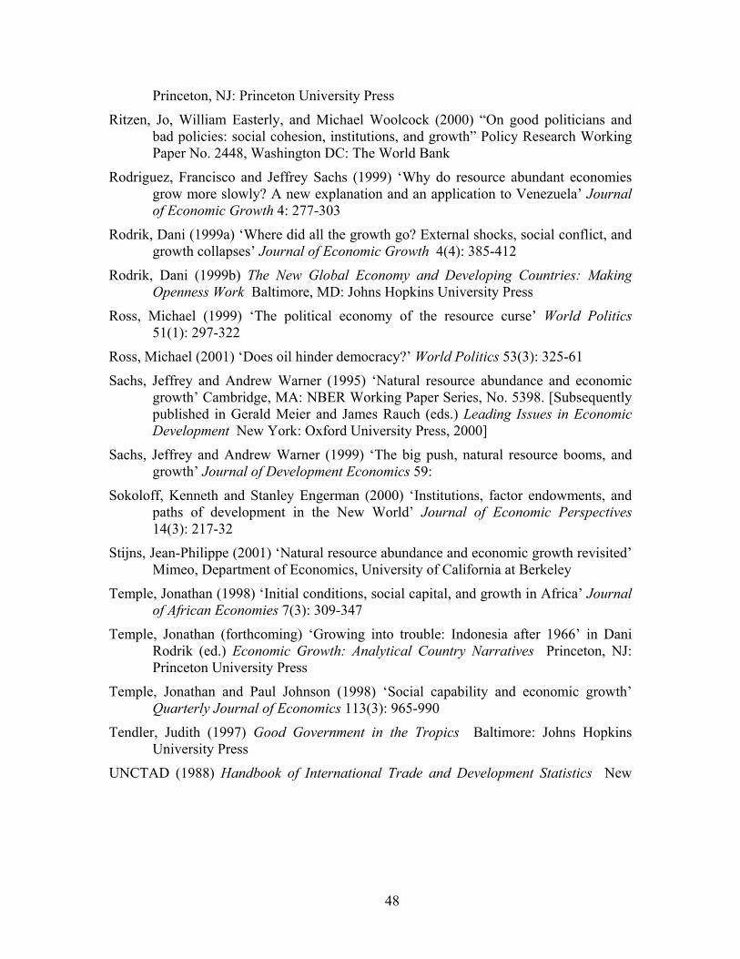
48

Princeton, NJ: Princeton University Press

Ritzen, Jo, William Easterly, and Michael Woolcock (2000) “On good politicians and bad policies: social cohesion, institutions, and growth” Policy Research Working Paper No. 2448, Washington DC: The World Bank

Rodriguez, Francisco and Jeffrey Sachs (1999) ‘Why do resource abundant economies grow more slowly? A new explanation and an application to Venezuela’ Journal of Economic Growth 4: 277-303

Rodrik, Dani (1999a) ‘Where did all the growth go? External shocks, social conflict, and growth collapses’ Journal of Economic Growth 4(4): 385-412

Rodrik, Dani (1999b) The New Global Economy and Developing Countries: Making Openness Work Baltimore, MD: Johns Hopkins University Press

Ross, Michael (1999) ‘The political economy of the resource curse’ World Politics 51(1): 297-322

Ross, Michael (2001) ‘Does oil hinder democracy?’ World Politics 53(3): 325-61

Sachs, Jeffrey and Andrew Warner (1995) ‘Natural resource abundance and economic growth’ Cambridge, MA: NBER Working Paper Series, No. 5398. [Subsequently published in Gerald Meier and James Rauch (eds.) Leading Issues in Economic Development New York: Oxford University Press, 2000]

Sachs, Jeffrey and Andrew Warner (1999) ‘The big push, natural resource booms, and growth’ Journal of Development Economics 59:

Sokoloff, Kenneth and Stanley Engerman (2000) ‘Institutions, factor endowments, and paths of development in the New World’ Journal of Economic Perspectives 14(3): 217-32

Stijns, Jean-Philippe (2001) ‘Natural resource abundance and economic growth revisited’ Mimeo, Department of Economics, University of California at Berkeley

Temple, Jonathan (1998) ‘Initial conditions, social capital, and growth in Africa’ Journal of African Economies 7(3): 309-347

Temple, Jonathan (forthcoming) ‘Growing into trouble: Indonesia after 1966’ in Dani Rodrik (ed.) Economic Growth: Analytical Country Narratives Princeton, NJ: Princeton University Press

Temple, Jonathan and Paul Johnson (1998) ‘Social capability and economic growth’ Quarterly Journal of Economics 113(3): 965-990

Tendler, Judith (1997) Good Government in the Tropics Baltimore: Johns Hopkins University Press

UNCTAD (1988) Handbook of International Trade and Development Statistics New

49

York: United Nations

Vick (2001)

Wade, Robert (1988) Village Republics: Economic Conditions for Collective Action in South India New York: Cambridge University Press

Weaver (2000)

Woolcock, Michael (1998) ‘Social capital and economic development: toward a theoretical synthesis and policy framework’ Theory and Society 27(2): 151-208

Woolcock, Michael and Deepa Narayan (2000) ‘Social capital: implications for development theory, research, and policy’ World Bank Research Observer 15(2): 225-249

Woolcock, Michael, Lant Pritchett and Jonathan Isham (2001) “The social foundations of poor economic growth in resource-rich economies” in R.M. Auty (ed.) Resource Abundance and Economic Development New York: Oxford University Press

World Bank (1998) Assessing Aid: What Works, What Doesn’t, and Why New York: Oxford University Press

World Bank (1999) World Development Indicators 99 Washington, DC: The World Bank

World Development (1996) Special issue on social capital and economic development. Vol 24(6).

Zak, Paul and Stephen Knack (1999) ‘Trust and growth’ Mimeo, Department of Economics, Claremont Graduate University

50

Appendix Table 1: Details on the export classifiactions derived from UNCTAD data

Export classification

Country Year Description of first and second most important exports

SIC export code for first

SIC export code for second

Percent of total exports

Percent of category exports

Manufacturing Bangladesh 1985 Woven textiles, textile 653 656 20, 19 65.8China 1985 Vehicles Parts, knitwear 784 845 6, 5 35.9Hong Kong ManufacturingIndia 1985 Pearl, clothing 667 841 11, 9 58Korea, Republic 1985 Ships, clothing 735 841 16, 14 91.3Nepal 1985 Floor cover, clothing 657 841 15, 12 59.1Singapore ManufacturingTaiwan, ChinaTurkey 1985 Clothing, Textile 841 651 16, 6 61

Diffuse Argentina 1985 Wheat, Oil seeds and nuts 041 221 13, 10 66.1Burma / Myanmar 1985 Rice, Wood 042 242 31, 33 56.5Gambia 1985 Oil seeds, veg oils 221 421 25, 21 84Guinea-Bissau FruitsHonduras 1985 Fruit, coffee 051 071 38, 25 84.7LesothoMalaysia 1985 Crude petrol, veg oil 331 442 23, 13 31.5Mali 1985 Cotton, Live animals 263 001 56, 30 58.6Mozambique 1984 Fish, fruit 031 051 36, 19 69Pakistan 1985 Cotton, rice 652 042 12, 12 61.9Panama 1985 Fruit, Fish 051 031 28, 21 78Philippines 1985 Special trans, Veg oil 931 422 30, 9 26.9Senegal 1985 Fish, Veg oils 031 421 14, 13 38Somalia 1985 Live animals, Fruit 001 057 79, 18 85.6Sri Lanka 1985 Tea, Clothing 074 841 39, 22 47.4Thailand 1985 Rice, Veg 042 054 13, 9 46.2Uruguay 1985 Wood, Meat 262 011 19.3, 14. 46.1Zimbabwe 1985 Tobacco, Pig Iron 121 671 23, 12 36.3

Point source Algeria 1985 Petroleum products, crude petrol 332 331 36, 32 97.6Angola 1985 Crude petrol, petroleum products 331 332 76, 5 84.9Benin 1982 Cotton, Cocoa 263 072 32, 27 46Bolivia 1985 Tin, gas 687 341 23, 52 55.7Botswana DiamondsBurkina Faso 1985 Cotton, Live animals 263 001 47, 13 56.8Chad 1980 Cotton, Live animals 263 001 61, 18 79.8Chile 1985 Copper, nonferrous ore 682 283 33, 10 58.3Congo 1985 Crude petrol, petroleum products 331 332 89, 4 93.3Dominican Repub. 1985 Sugar, pig iron 061 671 28, 14 42.7Ecuador 1985 Crude petrol, coffee 331 071 64, 7 66.7Egypt 1985 Crude petrol, cotton 331 263 51, 13 68.1Fiji SugarGabon 1985 Crude petrol, wood 331 242 84, 6 81.2

51

Appendix Table 1 (continued)Point source (continued) Guinea

GuyanaIndonesia 1985 Crude petrol, gas 331 341 48, 18 68.6Iran 1987 Crude petrol, tapestry 331 657 95, 2 95.8Iraq 1985 Crude petrol, fruit 331 051 95, 0 98.8Jamaica 1986 Inorganic elements, nonferrous me513 283 40, 20 51.9Jordan 1985 Fertilizers (crude), Fertilizer (manu271 561 35, 14 43.3Liberia 1985 Iron, rubber 281 231 63, 19 62.9Malawi 1983 Tobacco, tea 121 074 48, 24 96Mauritania 1985 Iron, fish 281 031 44, 40 58.3Mauritius 1985 Sugar, clothing 061 841 47, 29 49.8Mexico 1985 Crude petrol, petroleum products 331 332 56, 5 60Morocco 1985 Fertilizers, Inorganic elements 271 513 23, 16 40.5NamibiaNiger 1981 Uranium, live animals 286 001 81, 14 80Nigeria 1985 Crude petrol, cocoa 331 072 90, 2 96.7OmanPapua New Guinea 1985 Nonferrous metal, Coffee 283 071 35, 14 45.1Paraguay 1985 Cotton, Oil 263 221 43, 33 49.5Peru 1985 Petrol, nonferrous metal 332 283 16, 14 40.8Saudi ArabiaSierra Leone 1985 Pearl, Nonferrous metal 667 283 36, 26 34.8South Africa 1985 Special, Coal 931 321 54, 6 34.2Sudan 1985 Cotton, Oil Seeds 263 221 48, 15 71.3Syria 1985 Crude petrol, petroleum products 331 332 49, 19 74.1Togo 1985 Fertilizers, Cocoa 271 072 49, 16 53.6Trinidad & TobagoTunisia 1985 Crude Petrol, Clothing 331 841 40, 17 44.5Venezuela 1985 Crude petrol, petroleum products 331 332 46, 29 80Zaire 1985 Copper, Crude petrol 682 331 45, 22 44.2Zambia 1985 Copper, zinc 682 686 88, 2 93.4

Coffee/cocoa Brazil 1985 Coffee, petroleum products 071 332 10, 7 37Burundi 1985 Coffee, tea 071 074 84, 6 92.2Cameroon 1986 Coffee, cocoa 071 072 28, 22 52.5Central African Rep 1985 Coffee, Wood 071 242 35, 24 41.6Colombia 1985 Coffee, petroleum products 071 332 51, 13 59.3Costa Rica 1985 Coffee, fruit 071 051 30, 24 60.5Cote d'Ivoire 1985 Cocoa, Coffee 072 071 32, 25 68El Salvador 1985 Coffee, Sugar 071 061 63, 4 51.3Ethiopia 1985 Coffee, hides 071 211 63, 13 71.2Ghana 1985 Cocoa, Aluminum 072 684 66, 6 69.3Guatemala 1985 Coffee, Crude veg materials 071 292 35, 8 58.1Haiti 1985 Coffee, Clothing 071 841 27, 16 74.2Kenya 1985 Coffee, tea 071 074 27, 25 63.6Madagascar 1985 Coffee, spices 071 075 39, 29 79.2Nicaragua 1985 Coffee, Cotton 071 263 38, 33 58.2Rwanda 1985 Coffee, Tin 071 687 43, 9 76.4Tanzania 1985 Coffee, Cotton 071 263 39, 11 68.1Uganda 1985 Coffee, Hides 071 211 71.3, 6.9 90

Notes: Export classifications based on data from UNCTAD (1988) See the text for a description of the classification methodology

52

Appendix Table 2: Data sources and descriptions – TO BE FINALIZED Data type Series Description and source Natural resource base

All WDI material Series: Fuel exports (% of merchandise exports) (TX.VAL.FUEL.ZS.UN)

Fuels comprise SITC section 3 (mineral fuels). For more information, see WDI table 4.5.

Series: Agricultural raw materials exports (% of merchandise exports) (TX.VAL.AGRI.ZS.UN)

Agricultural raw materials comprise SITC section 2 (crude materials except fuels) excluding divisions 22, 27 (crude fertilizers and minerals excluding coal, petroleum, and precious stones), and 28 (metalliferous ores and scrap). For more information, see WDI table 4.5.

Series: Food exports (% of merchandise exports) (TX.VAL.FOOD.ZS.UN)

Food comprises the commodities in SITC sections 0 (food and live animals), 1 (beverages and tobacco), and 4 (animal and vegetable oils and fats) and SITC division 22 (oil seeds, oil nuts, and oil kernels). For more information, see WDI table 4.5.

Series: Manufactures exports (% of merchandise exports) (TX.VAL.MANF.ZS.UN)

Manufactures comprise commodities in SITC sections 5 (chemicals), 6 (basic manufactures), 7 (machinery and transport equipment), and 8 (miscellaneous manufactured goods), excluding division 68 (non-ferrous metals). For more information, see WDI table 4.5.

53

Series: Ores and metals exports (% of merchandise exports) (TX.VAL.MMTL.ZS.UN)

Ores and metals comprise the commodities in SITC sections 27 (crude fertilizer, minerals nes); 28 (metalliferous ores, scrap); and 68 (non-ferrous metals). For more information, see WDI table 4.5.

Series: Merchandise exports (current US$) (TX.VAL.MRCH.CD.WT)

Merchandise exports show the f.o.b. value of goods provided to the rest of the world valued in U.S. dollars. They are classified using the Standard International Trade Classification (SITC). Data are in current U.S. dollars. For more information, see WDI table 4.5.

Natural resource instruments

All Leamer material

All UNCTAD material

WP and I (2000)

Other instruments

Ethnic fractionalization

Ethnolinguistic fractionalization index (measures the probability that two randomly selected persons from a given country will not belong to the same ethnolinguistic group). Mauro (1997?), initially from the Atlas Narodov Mira (Department of Geodesy and Cartography of the State Geological Committee of the USSR, Moscow, 1964) and Taylor and Hudson (World Handbook of Political and Social Indicators, 1972)

Languages Hall and Jones 1999 Institutions CPIA Property rights and rule-based governance (CPIA)1998.

David Dollar et al.

Law and Order Tradition (ICRG)

Average 1984-1998. (scale 0-6, Lower point totals indicate higher risk)

Quality of the Bureaucracy (ICRG)

Average 1984-1998. (scale 0-6, Lower point totals indicate higher risk)

Political rights (Freedom House)

Average 1972-1998. (scale 1-7, 1 represents most free)

54

Civil Liberties (Freedom House)

Average 1972-1998. (scale 1-7, 1 represents most free)

Voice and Accountability

Kaufmann, Kraay and Zoido-Lobaton (1999a).

Political Instability and Violence

Kaufmann, Kraay and Zoido-Lobaton (1999a).

Government Effectiveness

Kaufmann, Kraay and Zoido-Lobaton (1999a).

Regulatory Burden

Kaufmann, Kraay and Zoido-Lobaton (1999a).

Rule of Law

Kaufmann, Kraay and Zoido-Lobaton (1999a).

Graft

Kaufmann, Kraay and Zoido-Lobaton (1999a).

Determinants of growth

The host of Barro-type x-country variables

Openness The openness measure …

Sachs and Warner (1995)