NBER WORKING PAPER SERIES

THE VALUE OF CONNECTIONS IN TURBULENT TIMES:EVIDENCE FROM THE UNITED STATES

Daron AcemogluSimon JohnsonAmir KermaniJames KwakTodd Mitton

Working Paper 19701http://www.nber.org/papers/w19701

NATIONAL BUREAU OF ECONOMIC RESEARCH1050 Massachusetts Avenue

Cambridge, MA 02138December 2013

We thank Isil Erel, Taylor Nadauld, and René Stulz for sharing data. For helpful comments we thankJosh Angrist, Caroline Hoxby, Suresh Naidu, Francesco Trebbi, and people who provided commentsduring or after our talks at MIT, Northwestern, Harvard Business School, the International MonetaryFund, the University of Alberta, BYU, Yale, the University of California at Berkeley, and the 2012Econometric Society meetings. We are also grateful for constructive suggestions from some formerofficials. The views expressed herein are those of the authors and do not necessarily reflect the viewsof the National Bureau of Economic Research.

At least one co-author has disclosed a financial relationship of potential relevance for this research.Further information is available online at http://www.nber.org/papers/w19701.ack

NBER working papers are circulated for discussion and comment purposes. They have not been peer-reviewed or been subject to the review by the NBER Board of Directors that accompanies officialNBER publications.

© 2013 by Daron Acemoglu, Simon Johnson, Amir Kermani, James Kwak, and Todd Mitton. Allrights reserved. Short sections of text, not to exceed two paragraphs, may be quoted without explicitpermission provided that full credit, including © notice, is given to the source.

The Value of Connections in Turbulent Times: Evidence from the United StatesDaron Acemoglu, Simon Johnson, Amir Kermani, James Kwak, and Todd MittonNBER Working Paper No. 19701December 2013JEL No. G01,G14,G21,G28

ABSTRACT

The announcement of Timothy Geithner as nominee for Treasury Secretary in November 2008 produceda cumulative abnormal return for financial firms with which he had a connection. This return was about6% after the first full day of trading and about 12% after ten trading days. There were subsequentlyabnormal negative returns for connected firms when news broke that Geithner’s confirmation mightbe derailed by tax issues. Excess returns for connected firms may reflect the perceived impact of relyingon the advice of a small network of financial sector executives during a time of acute crisis and heightenedpolicy discretion.

Daron AcemogluDepartment of Economics, E18-269DMIT77 Massachusetts AvenueCambridge, MA 02139and CIFARand also NBERdaron@mit.edu

Simon JohnsonMIT Sloan School of Management100 Main Street, E52-562Cambridge, MA 02142and NBERsjohnson@mit.edu

Amir KermaniHaas School of Business and Department of EconomicsUniversity of California, Berkeley2220 Piedmont AveBerkeley CA 94720amir@haas.berkeley.edu

James KwakUniversity of ConnecticutSchool of Lawjames.kwak@law.uconn.edu

Todd MittonMarriott SchoolBrigham Young University684 TNRBProvo, UT 84602todd.mitton@byu.edu

1 Introduction

On Friday, November 21, 2008, the news leaked that Timothy Geithner — then president

of the Federal Reserve Bank of New York — would be nominated by President-elect Barack

Obama to become Secretary of the Treasury of the United States. Over the next ten trading

days, financial firms with a connection to Geithner experienced a cumulative abnormal return

of about 12% (relative to other financial sector firms). When Geithner’s nomination ran into

trouble in January 2009, due to unexpected tax issues, there was a fall in the value of Geithner-

connected firms — although this effect is smaller and less precisely estimated than the increases

that were observed in November. How should we interpret these results?

This pattern seems unlikely to be a fluke of the data or a result of mismeasurement. We use

three different ways of identifying connections between financial institutions’ executives and

Geithner: (i) executives who had meetings with Geithner during 2007—08; (ii) executives who

belonged to the same nonprofit boards and groups as Geithner; and (iii) executives of firms

located in New York City, who would be close in proximity to the New York Fed. Our results

are essentially the same across all three measures of connections (although somewhat weaker

for the New York City measure), and they are robust across a wide range of checks, including

with various size controls and when we drop outliers.

Our results are also unlikely to reflect higher than normal returns for firms most affected

by the crisis and thus more likely to benefit from the appointment of a competent Treasury

Secretary. The results remain robust when we compare connected firms to non-connected firms

with similar size, profitability, leverage and prior stock price behavior, or when we control for:

how intensely firms were affected in the most severe phase of the crisis during September—

October 2008; how their stock price rose when capital was injected into big banks in October

2008; or how much they were exposed to troubled assets (in particular, residential mortgage-

backed securities). Episodes of purely supportive policy — such as the Bear Stearns rescue,

the AIG bailout, or the passage of the Emergency Economic Stabilization Act — did not cause

the same robust pattern of abnormal returns for Geithner-connected firms. We also examine

evidence on the market-perceived probability of bankruptcy from credit default swap spreads,

although the available sample for these data is smaller than for equities. We find the same

pattern in CDS spread data as in equity data — i.e., there was a perceived benefit to creditors (in

the form of lower implied default risk) when the firms’ executives were connected to Geithner.

There are at least three reasons why market participants may have expected benefits for

1

Geithner-connected firms. First, they may have expected that some form of explicit corruption

could take place. In countries with weak institutions and much policy discretion in the hands

of politicians, such as Indonesia, Malaysia, or Pakistan, potential corruption is a reasonable

interpretation of stock price movements for politically connected firms.1 But corruption is

not plausible as an explanation for what happened in the United States. Econometric results

that show large effects for political connections are typically based on data from countries

with weak institutions. In contrast, by most measures and at most times, the United States

has fairly strong institutions. Moreover, Geithner is widely regarded as an honest public

servant who is very unlikely to have acted on the basis of personal financial gain. Studies of

policymaking under the Obama administration by Suskind (2011) and Scheiber (2011) and first-

hand accounts by Bair (2012) and Barofsky (2012) — none of which are particularly sympathetic

to Geithner — contain absolutely no suggestion of corruption. Geithner has also never run for

public office and seems unlikely to ever do so, making political contributions irrelevant.2

Second, market participants may have believed that Geithner’s policy preferences were

generally consistent with the interests of the financial institutions with which he was connected.

This might have represented a type of “cultural capture” of key official decision-makers and

thinkers byWall Street (Bhagwati (1998), Johnson and Kwak (2011)). According to this theory,

instead of favoring firms because he had connections with them, Geithner’s prior connections

had already shaped his perspectives on the financial sector and on the crisis that was still

unfolding. In particular, his close connections to large, complex, Wall Street banks might have

persuaded him that broader economic prosperity required rescuing those banks on relatively

generous terms (for shareholders, as well as executives and creditors). Our results, however,

are not based on a comparison of financial to non-financial firms or of large relative to small

financial firms.3 Rather, as already noted, they are driven by a comparison of connected to

non-connected firms of similar size. Even if Geithner took the worldview that Wall Street

1For example, in a seminal study, Fisman (2001) found that being connected to President Suharto accounted

for 23 percent of firms’ value on average in Indonesia in the mid-1990s (where the events were rumors about the

president’s health). For Malaysia in the late 1990s, Johnson and Mitton (2003) found that connections to Prime

Minister Mahathir accounted for around 20 percent of firms’ total stock market value in a crisis, where the event

was the fall from power of Anwar Ibrahim, the Minister of Finance. Similar results are found in Pakistan by

Khwaja and Mian (2005), in a cross-country setting by Dinç (2005), and in Weimar Germany by Ferguson and

Voth (2008).2Duchin and Sosyura (2012) find that politically connected firms were more likely to receive TARP funds,

and also that such firms performed worse than non-connected firms. However, they measure connections to

Congress, not to Secretary Geithner.3Similarly, we show below that our results are not driven by Citigroup or other financial firms that are

considered by policymakers or markets as “too big to fail”. In all cases, we find that investors considered there

to be value in being personally connected to Geithner, quite aside from any “too big to fail” issues.

2

banks were “too big to fail”, this cannot directly account for our results.

Third, the market may have subscribed to a “social connections meets the crisis” hypothesis:

that connections would matter during a time of crisis and increased policy discretion. It was

perhaps reasonable to suppose that immediate action with limited oversight would have to be

taken, and that officials would rely on a small network of established confidantes for advice

and assistance. Powerful government officials are no different from the rest of us; they know

and trust a limited number of people. It is therefore natural to tap private sector friends,

associates, and acquaintances with relevant expertise when needed — including asking them for

advice and hiring them into government positions. Even with the best intentions, beliefs are

presumably shaped by self-interest, particularly when the people involved were, are, or will

be executives with fiduciary responsibility to shareholders. These tendencies can be checked

during ordinary times by institutional constraints and oversight, but during times of crisis and

urgency, social connections are likely to have more impact on policy.4

Our findings show a stronger effect for connections than is standard in most related research

on the United States.5 In part, previous studies have examined different kinds of connections,

focusing on the legislature, where the impact of a single individual is likely to be limited. For

example, the so-called Jeffords Effect — named after a Senator who switched parties unexpect-

edly, causing a change of control in the U.S. Senate — was found to be worth around 1% of firm

value (Jayachandran (2006)). Roberts (1990) found statistically significant but small effects on

connected firms from the unexpected death of a U.S. Senator. Fisman et al. (2012) studied the

value of connections to former Vice President Dick Cheney, driven by events such as his heart

attacks, surprise news about his political career, the original Bush-Cheney “hanging chad”

4Particularly important may have been Geithner’s connections through his long-term relationship with

Robert Rubin, who was Treasury Secretary in the Clinton administration, a former co-chair of Goldman Sachs,

and more recently a leading board member at Citigroup (he resigned from the latter position in January 2009).

From November 2003, Geithner was president of the Federal Reserve Bank of New York — an institution that

has traditionally served as the eyes and ears of the Federal Reserve on Wall Street, but which is sometimes con-

sidered to have become too much influenced by the thinking at large financial institutions. Formal responsibility

for supervision rests with the Board of Governors in Washington D.C., but the New York Fed is very much

engaged in collecting information and interpreting what is going on. By tradition, the president of the New York

Fed plays a particularly important role in managing relationships between government officials and financial

services executives who are based in New York (“Wall Street”, broadly defined). He is also, by convention, vice

chair of the Federal Open Market Committee, which sets monetary policy. (All presidents of the New York Fed

to date have been men.)5Akey (2013) presents findings that are similar in magnitude to ours, but for congressional elections where

“the wedge between firms connected to a winning politician and firms connected to a losing politician is 1.7%

to 6.8% of firm equity value.” Goldman, Rocholl, and So (2009) find that when George W. Bush won the

presidency in 2000 (and Republicans controlled the Senate and the House of Representatives), Republican-

linked firms gained 3%-5% relative to Democrat-linked firms, but the links they measure are not exclusive to

the executive branch.

3

presidential election victory in 2000, and Iraq war developments, and found no evidence of sig-

nificant effects. They concluded: “Contrary to conventional wisdom, we find that in all cases

the value of ties to Cheney is precisely estimated as zero. We interpret this as evidence that

U.S. institutions are effective in controlling rent-seeking through personal ties with high-level

government officials”.6

But Geithner ascended to the highest level of power at an unusual moment, with many

ideas in flux and great differences of opinion between otherwise well-informed and experienced

people.7 During the intense crisis of 2008 there was a wide range of opinions among policy

experts — and among potential Treasury Secretaries — regarding what should be done, with

significant potential implications for shareholders and creditors of financial institutions.

During such an episode where immediate action is necessary, it is plausible that the usual

institutional checks may not work and social connections may become more important as

sources of both ideas and manpower.8 This interpretation is also consistent with recent work

by Querubín and Snyder (2013). Using a regression discontinuity approach, they find that

American politicians were not able to enrich themselves before or after the U.S. Civil War, but

during the war there were substantial opportunities for personal gain — either because there

was more government spending or because news media were distracted or both.

Section 2 reviews the historical context and why market participants may have expected

connected firms to potentially perform better. Section 3 explains our coding of connections

and discusses the other variables we use. Section 4 presents our basic results and a range of

robustness checks. Section 5 analyzes the effects of Geithner’s tax issues, which temporarily

jeopardized his nomination in January 2009. Section 6 discusses the design and implementation

of bailout policy and financial reform under the Geithner Treasury. Section 7 concludes. The

Online Appendix (Tables A1 through A10) contains additional results and details on the data.

6Lower down the official hierarchy, there is certainly more rent-seeking behavior. For example, Dube, Kaplan

and Naidu (2011) find that (leaked) credible private information on coup attempts backed by the United States

does move stock prices.7There has always been lobbying in the United States, but other evidence suggests this may have been more

intense during the recent boom and bust, as the stakes became very high. Igan, Mishra, and Tressel (2011)

find that lobbying of legislators by lenders was associated with more risk-taking before the crisis and worse

outcomes in 2008, while Igan and Mishra (2012) examine how the political influence of the financial sector

affected deregulation. Mian, Sufi, and Trebbi (2010) establish that members of Congress were more likely to

support the Emergency Economic Stabilization Act of 2008 when they received higher contributions from the

financial services industry. Tahoun (2013) finds that members of Congress own stock in firms that contribute

to their campaigns, and that such firms receive more in government contracts.8Faccio (2006) finds connections of various kinds exist everywhere. Faccio, Masulis, and McConnell (2006)

show connected firms are more likely to receive bailouts across a wide range of countries, but the probability of

bailout is much lower in richer countries. See also Chiu and Joh (2004) and Dinç (2005).

4

2 The Context and Event

2.1 Historical Context

The financial crisis first became clearly evident in mid-2007 when problems with subprime

mortgages began causing major losses at some hedge funds and structured investment vehicles.

The crisis grew in severity during the spring and summer of 2008 — culminating in the collapse

of Lehman Brothers and a full-blown financial panic in mid-September.

These developments prompted Treasury Secretary Henry Paulson and Federal Reserve

Chairman Ben Bernanke to propose what eventually became the Emergency Economic Stabi-

lization Act (EESA), whose centerpiece was the $700 billion Troubled Assets Relief Program

(TARP).9 On October 14, 2008, using this legal authority, the Treasury Department, the Fed-

eral Reserve, and the Federal Deposit Insurance Corporation (FDIC) announced two measures

that began to calm the markets. First, they revealed that $250 billion of TARP money was

available to recapitalize financial institutions and, of this amount, $125 billion had already

been accepted by nine major banks. Second, there would be a program under which the FDIC

guaranteed new debt issued by banks.10 By mid-November, however, when President-elect

Barack Obama was selecting his Treasury Secretary, the crisis was far from over.

2.2 Channels of Influence

Why might market participants have believed that the nomination of Timothy Geithner as

Treasury Secretary would be good for Geithner-connected firms relative to non-connected

firms? There are two potential channels of influence that do not appear to operate. The

first possibility is some form of expected material compensation. One possibility could be

outright corruption, in which firms or their lobbyists pay officials directly for favors. As we have

already emphasized, there is no plausible evidence to suggest that the Geithner appointment

could have implied corruption. Geithner is known to be honest and the United States has

tough anti-bribery rules that remained effective even during the financial crisis.

9On September 18, 2008, Paulson and Bernanke provided a dramatic briefing to congressional leaders. Ac-

cording to Chris Dodd, then chair of the Senate Banking Committee, they were told “that we’re literally maybe

days away from a complete meltdown of our financial system, with all the implications here at home and glob-

ally.” David Herszenhorn, “Congressional Leaders Stunned by Warnings,” The New York Times, September 19,

2008. The initial Treasury proposal, published on September 20, was only three pages long and did not specify

any independent oversight mechanisms. “Text of Draft Proposal for Bailout Plan,” The New York Times, Sep-

tember 20, 2008. The initial legislative proposal was rejected by the House of Representatives on September 29.

An amended version passed and was signed into law on October 3, 2008.10“Joint Statement by Treasury, Federal Reserve and FDIC,” Treasury Department Press Release, October

14, 2008, available at www.federalreserve.gov/newsevents/press/monetary/20081014a.htm.

5

Another potential form of compensation is campaign financing, which sometimes matters

a great deal in the United States — particularly when elected officials have a sense of what

might encourage individual and corporate contributions to their campaigns. Geithner was

unelected and has never sought election, so such considerations are unlikely to be relevant in

his appointment or later decisions.

Material compensation also motivates the so-called “revolving door” between the public

and private sectors, in which government officials are friendly with firms they oversee and

subsequently — or perhaps consequently — secure lucrative positions with those firms. Yet

before his nomination to Treasury, Geithner already had ample opportunity to land highly

lucrative jobs in the private sector. It seems implausible to suggest that he was motivated —

or that anyone would think he could be motivated — by potential employment opportunities.

Second, there may well have been some “cultural capture” at the Treasury and in the

Obama administration, meaning the convergence of perspectives and interests that occurs

through immersion in a certain social or institutional context (e.g., working at the New York

Fed or being friends with high-profile financiers). Once in office, this shared mindset could

lead officials to decisions that favor the entire financial sector or perhaps some particular firms,

such as Wall Street banks. This is a plausible hypothesis in general, but the specific evidence

we present below cannot be explained by such cultural capture — our results indicate abnormal

returns for well-connected financial firms relative to other less well-connected firms with similar

characteristics, including size, profitability, leverage, and prior stock market performance.

One channel of influence that market participants in November 2008 could reasonably have

expected to apply relates to the role of social connections. Access to government officials

can be hugely beneficial, as witnessed by the large U.S. lobbying industry. When powerful

politicians make decisions, they may be influenced by the people they talk to — and the people

with whom they talk will likely be the people they know (Bertrand, Bombardini, and Trebbi

(2011), and Blanes-i-Vidal, Draca, and Fons-Rosen (2012)). In addition to the simplest form

of direct access through social connections — i.e., the fact that any official is more likely to take

a phone call from someone he knows than from a person he does not know — another form

of indirect access is provided by hiring. Any new administration must fill a large number of

important positions, and connections are an influential factor in hiring decisions.

By November 2008, Geithner knew the leaders of the New York financial community very

well, and it could reasonably be expected that he would continue to take their calls and listen

to them seriously as Treasury Secretary. He would also be expected to place people he knew

6

and trusted into important positions.11 Even if Geithner were not to favor connected firms

directly, they could still benefit through the influence of their alumni.

The “social connections meets the crisis” hypothesis implies that market participants might

expect Secretary Geithner’s appointment to favor financial institutions based on pre-existing

professional and social connections. Such positions might become even more valuable when

policy discretion is higher and very consequential decisions need to be made — such as during

the financial crisis that was raging in November 2008.

2.3 Policy Discretion in November 2008

As of November 2008, Congress had already explicitly granted broad powers to Treasury to

intervene in the financial sector, and Secretary Paulson had pressured nine major banks into

accepting $125 billion of new government capital.12 Although Paulson’s Capital Purchase

Program (CPP) distributed capital on relatively generous terms, access was tightly controlled

by Treasury. In late October, for example, PNC acquired National City after National City

learned that its CPP application might not be approved.13 At the time, there was little

transparency about how applications were reviewed and what criteria were being used to

determine which banks received capital. The Treasury Department determined who received

the benefit of both cheap capital and a government seal of approval (Veronesi and Zingales

(2010)).14

In addition, the Capital Purchase Program placed significant holdings of preferred stock in

the hands of the Treasury Department, as well as warrants on common stock. Although the

preferred stock was non-voting and Treasury committed not to vote its shares of common stock,

11We should emphasize that drawing on pre-existing relationships on Wall Street is well-established practice

for a Treasury Secretary, and did not begin with Geithner. For example, Henry Paulson brought in more and

more Goldman Sachs alumni as the crisis deepened, including Neel Kashkari, who was charged with running

TARP. Because of his expertise, Kashkari was initially kept on by Geithner.12Damian Paletta, Jon Hilsenrath, and Deborah Solomon, “At Moment of Truth, U.S. Forced Big Bankers to

Blink,” The Wall Street Journal, October 15, 2008.13Dan Fitzpatrick, David Enrich, and Damian Paletta, “PNC Buys National City in Bank Shakeout,” The

Wall Street Journal, October 25, 2008.14The investment terms were considerably more favorable than those available from the private sector, such

as in Warren Buffett’s investment in Goldman Sachs. According to Bloomberg, the government received war-

rants worth $13.8 billion in connection with its 25 largest equity injections; under the terms Buffett got from

Goldman, those warrants would have been worth $130.8 billion. In addition, TARP received a lower interest

rate (5%) on its preferred stock investments than did Buffett (10%). Mark Pittman, “Paulson Bank Bailout in

‘Great Stress’ Misses Terms Buffett Won,” Bloomberg, January 10, 2009. The TARP Congressional Oversight

Panel had similar findings. TARP Congressional Oversight Panel, “February Oversight Report: Valuing Trea-

sury’s Acquisitions,” February 6, 2009, available at www.gpo.gov/fdsys/pkg/CPRT-111JPRT47178/pdf/CPRT-

111JPRT47178.pdf. Although there were justifications for this subsidy — in particular, Treasury wanted broad

participation in order to avoid stigmatizing particular banks — it still constituted potential expected value that

the government was willing and able to transfer to specific financial institutions.

7

this still left open the prospect of increased government influence; participating institutions

were also subject to executive compensation and corporate governance requirements.15 The

mechanics of implementing TARP were run within Treasury, giving significant discretion to

the Treasury Secretary’s appointees.16

3 Data and Descriptive Statistics

Our sample consists of all firms trading on the NYSE or NASDAQ that are categorized as

banks or financial services firms in the Datastream database. Of these 678 firms, we exclude

those that lack sufficient stock return data in the Datastream or TAQ databases to calculate

abnormal returns for our Geithner announcement event. The remaining sample of 603 firms

we refer to as the “full sample”.

A potential complication is the Citigroup bailout which occurred between the news leak of

Geithner’s expected nomination on November 21 and the official announcement of his nomi-

nation on November 24, 2008. On Sunday, November 23, the U.S. government entered into a

bailout agreement with Citigroup that provided Citigroup with a $20 billion capital infusion

through TARP, as well as guarantees on a pool of $306 billion of troubled assets.17

Because the bailout occurred in the middle of the event window for the Geithner announce-

ment, and because the bailout (or at least the size and timing of the bailout) was not entirely

anticipated, it could complicate estimation of the effect of the Geithner announcement — at

least to the extent that there is correlation between firms connected to Geithner and firms

impacted by the Citigroup bailout news.18 In our tests, we address this issue in two ways.

First, we report results for stock price reactions on November 21 only, which is prior to the

Citigroup bailout announcement. While this approach avoids the confounding effects of the

15“TARP Capital Purchase Program: Senior Preferred Stock and Warrants,” available at on-

line.wsj.com/public/resources/documents/PublicTermSheet1014.pdf.16 In addition to Neel Kashkari, Reuben Jeffrey, another Goldman alumnus, was named as interim chief

investment officer, and several other ex-Goldman executives played important roles in the Paulson Treasury.

Julie Creswell and Ben White, “The Guys from ‘Government Sachs’,” The New York Times, October 17, 2008;

Deborah Solomon, “The Financial Crisis: Amid Turmoil, Tireless Team Of Advisers Backed Paulson,” The Wall

Street Journal, September 17, 2008.17“Joint Statement by Treasury, Federal Reserve, and the FDIC on Citigroup,” November 23, 2008, available

at www.federalreserve.gov/newsevents/press/bcreg/20081123a.htm18 It is not certain that a bailout would be positive news for Geithner-connected firms. We have tested the

effect of Geithner connections on returns surrounding another significant government bailout, the bailout of

Bank of America on January 16, 2009. The Bank of America bailout was similar in structure to the Citigroup

bailout, and confirmed the government’s willingness to take unprecedented measures to keep the largest banks

afloat. However, our tests show that cumulative abnormal returns for Geithner-connected firms surrounding

the Bank of America bailout are statistically insignificant, which suggests that Geithner-connected firms do not

generally have positive responses to the news of significant government bailouts of major banks.

8

Citigroup bailout, it is not entirely appealing because the post-leak return on November 21 is

only one hour in length, and because some uncertainty about the nomination remained until

the official announcement on November 24.

As a second approach, we exclude from our tests the firms that would be most likely to

be affected by the bailout announcement. We rank all firms in the sample based on their

return correlation with Citigroup during the period beginning the day of the Lehman collapse

and ending the day before the Geithner nomination announcement. We drop firms that rank

among the top 10% in correlation with Citigroup, and call this reduced sample our “base

sample”.19 To a large degree, the use of this base sample should eliminate the impact of the

bailout announcement on our estimates.

Table 1 reports summary statistics of our variables for political connections and financial

data. We identify connections to Geithner in three different ways. The first measure of

connections, which we refer to as “schedule connections”, identifies the number of times that

Geithner interacted with executives from each firm while he was president of the New York Fed.

We identify these interactions by searching Geithner’s daily schedule for each day from January

2007 through January 2009.20 For example, a search of Geithner’s schedule for Moody’s

Corporation reveals two interactions between Geithner and executives of Moody’s. On July 5,

2007, the schedule reads, “11:30 a.m. to 12:00 p.m. Meeting w/Raymond McDaniel, Chairman

& CEO, Moody’s Corporation”, and on September 15, 2008, the schedule reads “11:00 a.m.

to 12:00 p.m. Rating Agencies Meeting” and Raymond McDaniel is listed as one of the

participants. Based on this information, we code Moody’s schedule connections as two. Row

1 of Panel A of Table 1 reports descriptive statistics for this variable. By far the firm with

the greatest number of interactions listed on Geithner’s schedule is Citigroup, with a total of

34. Panel A of Appendix Table A1 lists all of the sample firms found on Geithner’s schedule

and the number of interactions. The average number of schedule connections, conditional on

a firm having at least one connection, is 4.96.

The second measure of connections to Geithner, which we refer to as “personal connec-

tions”, identifies the number of links that Geithner has with each firm through personal rela-

tionships. We identify these links using the relationship maps published by muckety.com (run

19We have also constructed the base sample by dropping firms that rank in the top 5% and in the top 20%

of those correlated with Citigroup. Our main results remain unchanged, although in the latter case only seven

firms remain in the treatment group.20“Geithner’s Calendar at the New York Fed,” The New York Times, available at

documents.nytimes.com/geithner-schedule-new-york-fed.

9

by independent journalists).21 The maps on muckety.com show the links for a given individual

to other people or to organizations.22 We count a link between Geithner and a firm if he has

a personal link with a person who is a director of the firm, or if he shares a board or similar

position (e.g., trustees of the Economic Club of New York) with someone who works for the

firm.23 We require that those links be active when Geithner’s nomination was announced.

For example, we find a link between Geithner and American Express on muckety.com

through Kenneth Chenault, chairman and CEO of American Express, who is associated with

Geithner through the National Academy Foundation, where they are both directors, and

through the Partnership for New York City, where Chenault is a vice chairman and Geithner

is a board member. Based on this information we code personal connections for American Ex-

press as one. Descriptive statistics for this variable are reported in Row 2 of Table 1. Geithner

has the greatest number of personal connections (nine) to Citigroup; in contrast, he has only

one connection to Bank of America. The average number of personal connections to Geithner,

conditional on a firm having at least one connection, is 2.24. Appendix Table A2 lists all of

the identified personal connections between Geithner and sample firms.

To independently verify the accuracy of the information provided by muckety.com, we

searched the annual reports of each company with an identified personal connection to Gei-

thner, as well as other publicly available information. We were able to verify 52 of the 58

connections reported by muckety.com, 45 of those using the annual report filed most im-

mediately subsequent to the Geithner nomination announcement (typically, for years ending

December 31, 2008), and another seven using other sources such as Forbes and Bloomberg. Of

the remaining six connections, two are confirmed to be errors and are excluded from our data.

The other four are identified as legal counsel for financial firms in the sample. These have also

been excluded from our data due to the difficulty of verifying the connection and because of

the different nature of the connections. These exclusions leave us with a set of 52 personal

connections to Geithner from 21 different financial firms (although five connected people each

have two board links to Geithner). Panel B of Appendix Table A1 lists these firms and their

connections.

21These data are broadly similar to what is available for emerging markets, e.g., Gomez and Jomo (1997,

1998) on Malaysia. Many connections in emerging markets are formed early in careers. Most of the Geithner

connections are from his time at the New York Fed. We use muckety.com relationship maps from March 2009.22Measuring connections in ths way is standard in the network sociology literature. See, for example, Useem

(1984). Fisman et al. (2012) review the sociology literature on why board ties matter, including for the flow of

information.23Most of our data are board memberships, which are a matter of public record. However, the muckety.com

coding also contains some well-known mentor/adviser relationships, with Robert Rubin and a few others.

10

The third measure of connections to Geithner is based on firm location, under the reasonable

assumption that Geithner would have greater contact with executives of firms headquartered

in New York City, where Geithner was located as president of the New York Fed. This measure

is a dummy variable set equal to one if the headquarters of the firm is identified as New York

City in the Datastream database. Descriptive statistics are reported in Row 3 of Table 1.

Forty-five of the sample firms have headquarters in New York City; these firms are listed in

Appendix Table A3. All other sample firms not listed in Appendix Table A3 are listed in

Appendix Table A4.

As is shown in Appendix Tables A1 and A3, there is some overlap in the three measures

of connections. Of the 63 firms that have some measure of connections, nine are connected

according to all three measures, ten are connected according to two of the three measures,

and 44 are connected according to only one of the measures. In subsequent analysis, when

regressions include our standard control variables, the number of connected firms becomes 22

(schedule), 20 (personal), and 41 (New York) due to missing data on control variables. In

addition, when we focus on our base sample the number of connected firms is 12 (schedule), 8

(personal), and 34 (New York).

Rows 4 through 6 of Panel A of Table 1 report basic financial information for the sample

firms as obtained from the Worldscope database for the year 2008. Size (Row 4) is reported

as the logarithm of total assets, profitability (Row 5) is return on equity, and leverage (Row

6) is the ratio of total debt to total capital. Rows 7 through 9 report summary statistics for

our primary measure of firm performance, cumulative abnormal stock returns (CARs) — the

calculation of which is discussed in the next section. Rows 10 through 12 report statistics

for our secondary measure of performance, percentage changes in credit default swap (CDS)

spreads, which is also covered in the next section.

Panel B of Table 1 reports differences in the means of these variables between firms con-

nected to Geithner and non-connected firms; here his schedule and personal connections are

converted to a dummy variable equal to one for firms that have any connection. Row 13 of Panel

B shows that connected firms are significantly larger than non-connected firms for all three

measures of connections. Row 14 shows that profitability is significantly lower for connected

firms, but only when we use the New York measure. Row 15 shows that leverage is higher for

connected firms, but the difference is only significant for the schedule measure of connections.

Panel C repeats the analysis of Panel B for the base sample. The differences reported in Panel

C are broadly similar to those in Panel B. Because of the performance differences shown in

11

Panels B and C, we control for these variables below. Finally, Panel D of Table 1 reports

correlation coefficients between the explanatory variables reported in Panel A.

4 Geithner Connections and Stock Returns

In this section we study whether connections to Geithner, as defined in the previous section,

are associated with differences in returns at the time of the announcement of Geithner’s nom-

ination. We begin by calculating returns for each firm in the sample on the relevant dates.

Geithner’s nomination was officially announced by President-elect Barack Obama early on

Monday, November 24, 2008. However, news of his impending nomination was leaked to the

press late in the trading day on Friday, November 21, 2008 at approximately 3:00 p.m. ET —

a time that coincides with the beginning of a stock market rally.

For the purposes of studying stock price reactions, we define event day 0 as November 21 and

event day 1 as November 24, with subsequent event days corresponding to subsequent trading

days. We obtain daily stock returns for each sample firm from the Datastream database. In

order to more precisely delineate the response to the Geithner announcement on event day 0,

we calculate returns on that day as only the returns from 3:00 p.m. until the market close at

4:00 p.m. We obtain intraday returns from the TAQ database.

4.1 Univariate Tests

Panel A of Table 2 compares actual returns between connected and non-connected firms in the

base sample for event days 0 through 10. Panel A shows that on event day 0, using schedule

connections, connected firms outperformed non-connected firms by 4.3 percentage points, a

difference that is significant at the 5% level. Results are similar for the other measures of

connections, though not statistically significant for personal connections. On event day 1, when

the nomination was officially announced, return differences are even more pronounced. Using

the schedule measure, connected firms outperformed non-connected firms by 8.4 percentage

points on this day. The corresponding outperformance for firms with personal connections is

9.6 percentage points, and for firms with New York connections it is 3.1 percentage points.

The difference for the schedule and personal connections is significant at the 1% level, while

for New York it is significant at the 10% level.

Panel A also shows that connected firms continued to outperform non-connected firms on

each day through event day 10, with the primary exception being event day 5.24 The final row

24The underperformance of connected firms on event day 5 (a day when there was a sharp market down-

12

of Panel A reports cumulative performance for event days 0 through 10. Using the schedule

measure of connections, connected firms outperformed non-connected firms by 37.1 percentage

points over this period. For personal connections the difference was 46.3 percentage points,

and for New York connections the difference was 29.9 percentage points. By any measure of

connections, the outperformance of connected firms over this period was economically large

and highly statistically significant.

Because there were large market movements during the event window, it is important to also

calculate abnormal returns for the event days. Our procedure for calculating abnormal returns

follows Campbell, Lo, and MacKinlay (1997). We calculate cumulative abnormal returns using

the market model as follows:

[0 ] =

X=0

where [0 ] is the cumulative abnormal return for firm for event days 0 through .

is calculated as

= − [̂ + ̂]

where is the abnormal return for firm on event day , is the actual return on firm

for event day , and is the return on the market for event day , with the market return

represented by the return on the S&P 500 index. The parameters ̂ and ̂ are estimated

from the following equation:

= + +

on a pre-event period of 250 trading days ending 30 days prior to event day 0. Although the

choice of estimation period length is subjective, a length of 250 days corresponds to roughly

one year of trading and has been used in other studies such as Jayachandran (2006) and Li

and Lie (2006). The cumulative abnormal returns show the actual returns of each firm less the

predicted returns of each firm based on that firm’s performance relative to the market over the

estimation period.25

Panel B of Table 2 compares cumulative abnormal returns between connected firms and

non-connected firms in the base sample for event days 0 through 10. In contrast to the actual

returns reported in Panel A, no significant difference is reported between CARs of connected

firms and non-connected firms for the one hour of event day 0. Beginning on event day

turn) applies only to actual returns. In terms of abnormal returns (discussed below), there is no significant

underperformance of connected firms on event day 5.25We also calculated abnormal returns using a three-factor model, but the improvement in fit relative to the

market model was negligible.

13

1, the differences in CARs between connected firms and non-connected firms are relatively

large, but not statistically significant. Significant differences in CARs increase on subsequent

event days. The final row of Panel B shows that using the schedule measure, [0 10] for

connected firms is higher than [0 10] for non-connected firms by 15.7 percentage points.

The corresponding differences for the other measures are 15.8 percentage points and 11.0

percentage points, and in all cases the difference between the CARs is significant at the 1%

or 5% level. We repeat the analysis of Table 2 for the full sample and report those results in

Appendix Table A5. The results are fairly similar to those reported for the base sample.

Table 2 shows strong performance of connected firms relative to non-connected firms in

response to Geithner’s nomination as Treasury Secretary. In the tests that follow, we assess

whether these results hold when controlling for other firm characteristics in a multivariate

setting.

4.2 OLS Regression Results

To control for additional characteristics of the sample firms, we first test the relationship

between connections to Geithner and cumulative abnormal returns in a regression framework.

We estimate the following equation:

= + + z0φ+ (1)

where is either [0], [0 1], or [0 10] for firm , is a measure of connec-

tions for firm , and z is a set of firm-level covariates for firm (such as firm size, profitability,

and leverage).

The firm-level covariates are included to control for other basic firm characteristics that

could have some effect on the observed relationship between connectedness and returns. A

common practice in regressions of this type in previous literature is to not control for firm-

level characteristics (see, e.g., Fisman (2001), Jayachandran (2006), Fisman et al. (2012)),

although Johnson and Mitton (2003) control for firm size and leverage and Jayachandran

(2006) controls for firm size in robustness checks.

Results from such regressions could be confounded, however, by the differential effects of

events following Geithner’s nomination on firms with different characteristics. For this reason,

in the regressions that follow we control flexibly for a range of firm-level characteristics —

and, as a further step in this direction, we will also report results from various matching

estimators. In particular, firm size is included as a control because if Geithner had more

14

interaction with larger firms — and Panel B of Table 1 indicates that this is the case — then the

observed performance of Geithner-connected firms could be due to their size rather than to

their connections. Profitability is also an important control because it is an indicator of how

hard each firm had been impacted by the crisis, and it is possible that the firms that had been

hit the hardest also had the most to gain from Geithner’s appointment. Finally, leverage is

included as an additional indicator of the vulnerability of each firm during the crisis. For all of

these variables, we include cubics — i.e., the level, square, and cubed value — so as to account

for potential non-linear effects.

There might be other factors causing correlation of error terms (residual returns) across

firms. Unadjusted OLS standard errors would be biased in this case and could be too low.

To adjust for this possibility, we estimate adjusted standard errors that account for potential

cross-firm correlation of residual returns. We estimate the covariance matrix of returns using

pre-event return data on a window of 250 trading days ending 30 days prior to event day

0. This estimated covariance matrix is then used to calculate our standard errors, under the

assumption that the pre-event covariance matrix is an appropriate estimate of the covariance

matrix during the event. These adjusted standard errors should account for observed cross-

sectional correlation of returns between firms in our sample (see Greenwood (2005); Becker,

Bergstresser, and Subramanian (2013)). We use these adjusted standard errors below.

Table 3 reports results of the estimation of equation (1). The adjusted standard errors

are reported below coefficients in parentheses. The three measures of Geithner connections

(schedule, personal, and New York) are tested in turn. Although there is no established

standard in the literature for the appropriate length of the event window, we follow the practice

of first reporting results for shorter event windows ([0] and [0 1]) and then a longer

event window ([0 10]). The first three columns of the table report results for the full

sample with [0] as the dependent variable — the Citigroup bailout occurred after the

first trading day and thus correlation with Citigroup is not a concern when we use [0]. In

Column 1 the coefficient on schedule connections is 0.0033, which indicates an abnormal return

of over 0.3% for each additional connection and is statistically significant at the 1% level. So,

for example, a firm with a number of connections equal to the sample average, conditional

on being connected (4.96 connections in the full sample), would have had an abnormal return

of roughly 1.6% on average, relative to non-connected firms during the last hour of trading

on November 21. The coefficient on personal connections is significant at the 5% level and

indicates an abnormal return of over 0.7% for each additional personal connection, which also

15

implies a similar average abnormal return of about 1.6% for the average connected firm (which

has 2.24 personal connections in the full sample). The coefficient on New York connections is

significant at the 10% level and indicates that firms with New York connections had abnormal

returns of 1.3% relative to non-connected firms.26

Columns 4 through 6 of Table 3 report results for [0 1] focusing on the base sample.

The coefficients on schedule connections and personal connections are both positive and signif-

icant at the 1% level. The magnitude of the coefficient on schedule connections indicates that

each additional interaction with Geithner during his tenure at the New York Fed is associated

with an abnormal return of 1.1% for event days 0 and 1 combined. This implies an abnormal

return of about 3.5% for the average connected firm (which has 3.16 schedule connections in

the base sample). The coefficient on personal connections indicates an abnormal return of 5.0%

for each additional personal connection between Geithner and the firm, and thus an abnormal

return of about 8.8% for the average connected firm (which has 1.75 personal connections in

the base sample). The coefficient on New York connections is not statistically significant.

The last three columns of Table 3 report results for the estimation of equation (1) on the

base sample with [0 10] as the dependent variable. In these three columns the coefficient

on Geithner connections is positive for all measures and significant at the 1% level for the

personal and New York measures. Compared to the quantitative magnitudes for [0 1],

the coefficients on the personal and schedule measures are similar, but the coefficient on the

New York measure is much larger, showing an abnormal return of 10.8% for connected firms.

In summary, Table 3 reports economically meaningful and statistically significant cumula-

tive abnormal returns for Geithner-connected firms following the announcement of his nomi-

nation as Treasury Secretary, for both short and long event windows.27

4.2.1 Robustness Checks for OLS Results

We perform additional tests to assess the robustness of our baseline results reported in Table

3, and these are presented in Table 4. In this table and in others that follow, we suppress

reporting of the coefficients of control variables for brevity, although we always include the

control variables (up to cubics in size, profitability, and leverage) in all specifications. To save

space we do not report results for New York connections in this table.

26We do not report results for the base sample for [0], but the corresponding coefficients in the base

sample are positive for all three measures and statistically significant for the New York measure.27We do not report results for the full sample for [0 1] and [0 10], but the corresponding coefficients

in the full sample are generally larger and more precisely estimated than those reported for the base sample.

16

We first address the question of whether Geithner-connected firms performed well after the

announcement of his nomination because of their personal connections to Geithner or because

Geithner’s appointment represented a signal that economic policy would be sensible. We get

at this question in four ways.

Our first set of robustness checks controls for the vulnerability of firms to the macroeco-

nomic conditions prevailing at the time. These include the extent to which firms’ stock prices

declined in the immediate aftermath of the collapse of Lehman Brothers in September 2008 —

as a measure of how badly a firm might have suffered from the uncertainty or the fire sales

that a further collapse could have triggered (and that Geithner’s policies might have been

anticipated to mitigate). Specifically, we calculate the cumulative abnormal return starting on

the day of Lehman’s bankruptcy (Monday, September 15, 2008, is day 0 for this event) and

for the following four days, which comprises the entire trading week.

As a second way to measure crisis vulnerability, we control for whether the firm is a deposit-

taking institution, as such institutions may have differed in vulnerability to the crisis from other

financial firms. Using Worldscope data, we create a dummy variable for positive deposits.

Finally, we also control for whether firms had already received TARP funding prior to the

announcement of Geithner’s nomination, which can act as another proxy for the systemic

importance of a firm. TARP-approved firms were unlikely to collapse.

Columns 1 and 2 of Table 4 report results controlling for all three of these proxies for crisis

vulnerability. The results are similar to our baseline results, with the exception that results for

[0 10] are somewhat weaker (Panel C). The coefficients on the proxies for crisis vulnera-

bility (not reported in the table) are not always statistically significant in the regressions, but

the coefficients on the Lehman bankruptcy CAR and the deposit-taking dummy are generally

negative, and the coefficient on the TARP-funding dummy is generally positive.

In Columns 3 and 4 we control for how firms responded to the announcement in early Oc-

tober that TARP funds would be used to recapitalize large banks. This decision was generally

regarded as the best of the available alternatives — so the response to this announcement offers

another plausible way to control for how firms were affected by sound policy decisions. This

decision was made public on Monday, October 13, with the announcement just after the stock

market closed — although it followed a meeting of top bankers at the Treasury Department

that was public knowledge. Similar European recapitalization plans had been unveiled over

the weekend, and this further contributed to the expectation that something similar would

happen in the United States. We calculate [0 1] for this event with October 13 as day

17

0 and October 14 as day 1. Columns 3 and 4 show that controlling for this variable in our

regressions does not alter the main results. The effect of being connected to Geithner remains

statistically significant.

As a third approach we recalculate abnormal returns using an estimation window that is

focused on the turbulent period surrounding Lehman’s collapse — so our measure of expected

returns uses betas that reflect the response of each firm to market movements during this par-

ticular period. We calculate abnormal returns as described above, except that the estimation

period begins two weeks prior to the Lehman collapse (Monday, September 1, 2008) and ends

three weeks after the Lehman collapse (Friday, October 3, 2008), when Congress ultimately

approved EESA (which included TARP). Results using this measure of abnormal returns are

reported in Columns 5 and 6. The results show that the coefficients on Geithner connections

are significant across all three panels in this specification and are all larger in magnitude than

the coefficients in our baseline results.

As a fourth approach, in Columns 7 and 8, we control more directly for the exposure of

financial firms to “toxic assets”. We measure exposure to toxic assets using data from Erel,

Nadauld, and Stulz (2013). We use their measure of holdings of mortgage-backed and asset-

backed securities (scaled by total assets) compiled from the Consolidated Financial Statements

for bank holding companies, as reported by the Federal Reserve Board of Governors. We use

data as of December 2008, and the variable is available for only 196 insured banks in our

sample. When controlling for this variable, the coefficient on Geithner connections is highly

significant in all three panels. The coefficient on “toxic assets” (not reported in the table) is

always positive and usually significant.28

In our next robustness checks we test for the influence of the largest firms and extreme

observations on our results. Although we control flexibly for firm size throughout our analysis,

in Columns 9 and 10 we take another approach by limiting the sample to only the top size

decile of sample firms, thereby creating a subsample that is more homogenous in terms of size.

The coefficient on Geithner connections is positive and statistically significant in four out of

six cases in this subsample.

In Columns 11 and 12 we exclude firms that the administration deemed to be of systemic

importance, in that they were later included in the government-administered stress tests. The

28We have also examined the effect of including interactions between our various measures of exposure to a

further decline in asset prices (i.e., the control variables in Columns 1 through 4 and Columns 7 and 8) with the

Geithner connection variable. There are in general no robust and consistent interaction effects between these

exposure variables and connections to Geithner.

18

firms that the government included in the stress tests (i.e., the Supervisory Capital Assessment

Program, SCAP) were those viewed in early 2009 as systemically important by the administra-

tion — and thus may have been more likely to benefit from bailouts similar to the one provided

to Citigroup or from other policies.29 These estimates are positive and significant in all but

one case. In Columns 13 and 14 we check for the influence of outliers by excluding firms

with extreme CARs, defined as those larger than the 99th percentile or smaller than the 1st

percentile. The Geithner coefficient is significant in all but one case in this specification.

As an additional robustness test, we consider whether results obtained for the schedule

measure of connections are robust when we calculate the number of connections using only

Geithner’s appointments from the year 2007. By 2008, the initial stages of the crisis were un-

derway, so Geithner may have had an increased number of meetings during this time with firms

affected by the crisis. Using only 2007 appointments as the schedule measure of connections

puts the focus on pre-crisis relationships. The results using the 2007 measure are reported in

Column 15. As with our baseline results, the coefficient on schedule connections is significant

at the 1% level for [0] and [0 1], but not for [0 10].

To summarize, in the robustness checks in Table 4 the Geithner connection coefficients gen-

erally retain statistical significance, although there are some exceptions. The magnitudes of the

coefficients vary but are often larger than those reported in the corresponding baseline results

in Table 3. Table 4 indicates the positive relation between Geithner connections and abnormal

returns surrounding his nomination announcement is fairly robust in OLS specifications.30

We also estimate similar results using various matching estimators. This includes propen-

sity score matching estimators in which firms were matched just on size; on primary control

variables (size, profitability and leverage); and on primary control variables plus other con-

trol variables (TARP participation dummy, deposit-taking dummy, and the CAR surrounding

the Lehman collapse). It also includes a nonparametric matching estimator, which estimates

the impact of connections on cumulative abnormal returns separately across 64 cells created

according to the covariates values and then combines them using the inverse standard errors

29This excludes the following 17 firms from our sample: American Express, Bank of America, BB&T, Bank

of New York Mellon, Capital One, Citigroup, Fifth Third Bank, Goldman Sachs, JPMorgan Chase, Key Corp.,

Morgan Stanley, PNC Financial Services, Regions Financial, State Street, SunTrust, U.S. Bancorp, and Wells

Fargo. The other two SCAP participants, GMAC and MetLife, are not part of our sample.30To briefly summarize the results for the unreported New York measure of connections, it is statistically

significant (with the expected sign) in the following specifications: in Panels A and C when controlling for crisis

vulnerability, in Panels A and C when controlling for the TARP capital injections, in all three panels when

using the Lehman collapse beta, in Panel B when controlling for toxic assets, in Panel C when using the top

size decile only, in Panels A and C when excluding systemically important firms, and in Panels A and C when

excluding outliers.

19

of the estimates as weights. These results, which are reported in Appendix Table A6, show a

similar pattern to that found in our other robustness checks.

4.3 Synthetic Matching Methodology

The results presented so far — and most event studies of this type — implicitly assume that

the differences between the treatment group (Geithner-connected firms) and the control group

(non-connected firms) can be captured by a combination of the excess return calculation and

the covariates included in the regression model. But connected and non-connected firms may

be different in other ways, which might be, at least partially, responsible for our results.

As a complementary approach to address these concerns, we turn to the method of synthetic

matching developed in Abadie and Gardeazabal (2003) and Abadie, Diamond, and Hainmueller

(2009). The main idea of this method is to construct a synthetic match for each firm in the

treatment group (i.e., firms connected to Geithner) by using the firms in the control group in

such a way that the synthetic firm has similar behavior to the actual firm before the event of

interest. In contrast to the OLS results with flexible controls and the propensity score matching

and nonparametric estimates discussed above, which compare firms that are similar in terms

of the covariates, this approach compares firms that are similar in terms of the behavior of

their pre-event abnormal returns.

The effect of the event can be measured as a function of the difference between the behavior

of the firm and its synthetic match after the event. Abadie, Diamond, and Hainmueller (2009)

show that a primary reason to use this method is to control for the effect of unobservable

factors that have an impact on the common time trend in the treatment and control groups.

Most previous papers employ synthetic matching for the case of one entity in the treatment

group and one intervention. Since our sample includes many connected firms, we extend this

method for the case of many firms in the treatment group. As we explain below, inference is

based on confidence intervals we construct from the distribution of the “Geithner effect” for

placebo treatment groups on Geithner’s nomination.31

More formally, our synthetic matching procedure is as follows. First, we divide the firms

into treatment and control groups according to our measures of connections to Geithner. Then

we construct a synthetic match for each firm in the treatment group by solving the following

31These intervals are constructed for testing the hypothesis of whether the effect of Geithner connections is

zero or not — and are thus not standard confidence intervals.

20

optimization problem:

∀ ∈ {∗ }∈ = argmin

{}∈

X[ −

X]

2

∈ ∈

X

= 1

∈ and ∀ ∈ ∀ ∈

≥ 0

where is the daily return on date and is the weight of control firm employed in the

optimal weighting for firm . It is important that the estimation window not include the period

of intervention and it is typically selected as some period prior to the intervention. As before,

we use 250 trading days ending 30 days prior to the Geithner nomination announcement as our

estimation window.32 The two criteria (P

= 1 and

≥ 0) imply the return for firms inthe treatment group belong to convex combinations of returns for firms in the control group.

After finding the optimal weights through iteration for each firm in the treatment group,

the return for the synthetic firm is constructed as:

c =X

∈

and the abnormal return is computed as the difference between the actual return and the

synthetic firm return (c).

To estimate the effect of intervention, we compute:

b( ) =P

∈

=0

−P∈

1

where

b =vuut P

∈

[ − c]2

In the above formula, b( ) is the effect of intervention at date computed using cu-

mulative abnormal returns of dates [ + ], 1 b is a measure of goodness of the match inthe estimation window, and is the length of the estimation window. This formula for the

average effect of intervention on the treatment group is thus a weighted average formula, with

greater weight given to better matches. This is because the difference between actual returns

32We find that the main results are robust to using other estimation windows. The results are somewhat

stronger when we use estimation windows closer to Geithner’s nomination starting from September 2008.

21

and synthetic firm returns should contain more information about the intervention when we

are better able to predict the return of the firms during the estimation window.

To construct the confidence intervals, we randomly draw 5,000 placebo treatment groups

from the control group — with each group having the same size as the real treatment group.

We compute the Geithner-connection effect for these placebo treatment groups on event days,

and construct the confidence intervals for hypothesis testing of whether the coefficient is sig-

nificantly different from zero. The effect of Geithner connections is significant at 5% if it does

not belong to the interval that contains the [2.5, 97.5] percentiles of the effect of the Geithner

connection for placebo treatment groups.

Table 5 presents the results from the synthetic matching estimation. Because synthetic

matching requires a dichotomous definition of the treatment and control groups, we also con-

sider two additional definitions of connections: “highly connected” firms, which are defined as

those with more than two identified meetings with Geithner, and “mildly connected” firms,

which are those with one or two identified meetings.33

Panel A of Table 5 presents results for the full sample in [0], and Columns 1 through 3

present results for all Geithner schedule connections (highly and mildly connected). Column 1

reports standard OLS results. In order to be comparable to the synthetic matching results, the

connections variable is a dummy (equal to one for firms with any number of connections). We

continue to adjust the OLS standard errors for pre-event correlations between firms, and the

OLS regressions include cubics in size, profitability, and leverage as before. Column 1 shows

that Geithner connections are associated with an abnormal return of 1.4% for the one-hour

return on day 0, and that this coefficient is statistically insignificant. Below the coefficient we

report the number of significant coefficients obtained at each significance level when we test

the effect of Geithner connections on 100 trading days between October 31, 2008, and April 7,

2009 (excluding key event dates), a period that does not overlap with our estimation period.

The number of significant coefficients on non-event days indicates the drawback of using OLS

— i.e., the Geithner connections coefficient is significant more often than would be expected.

Column 2 presents the synthetic matching results as outlined above. The coefficient on

33Appendix Table A7 reports the weights on firms in our control group for each firm in our treatment group.

Our control group includes synthetic matches based on the characteristics of over 70 firms. For example, in

the synthetic match for Bank of America, Wells Fargo contributes a weight of 0.30. But Wells Fargo is not a

particularly good match for other firms in our treatment group — it contributes a weight of 0.19 for JPMorgan

Chase but not more than a 0.06 weight for any other firm. U.S. Bancorp contributes a weight of 0.41 for PNC,

but this is unusually high. The pattern for Citigroup is more common — one firm contributes a weight of 0.21

to the synthetic match, another eight firms contribute weights of between 0.08 and 0.13, and one other firm has

a weight of 0.01.

22

Geithner connections is smaller than in the OLS results and is not statistically significant.

The number of significant coefficients shows that in the non-event-day tests, the Geithner

connections coefficient is significant with a frequency that is much closer to what would be

expected in theory (e.g., at the 5% level, four times in a test window of 100 trading days).

This makes us more confident that in the synthetic matching method we are isolating the true

effect of Geithner connections rather than the effect of some other correlation among Geithner-

connected firms (which would have led to more frequent rejections on non-event days).

Column 3 presents “corrected” synthetic matching results in which for our inference proce-

dure we eliminate firms for which we do not have a good synthetic match, defined as the firms

in the control group with b more than √3 times the average b for the real treatment groupfirms.34 Although the formula used in the synthetic matching method already gives greater

weight to firms with better matches, we present the corrected results as a robustness check

to ensure that our confidence intervals are appropriate. The corrected results are similar to

the uncorrected results in Column 2. Columns 4 through 6 present a similar set of results

for the “highly connected” indicator, and Columns 7 through 9 for the “mildly connected”

indicator. As expected, the results are stronger for highly connected firms. Overall, Panel A

suggests that the effect of Geithner connections on the one-hour day 0 returns is positive but

not statistically significant once the synthetic matching adjustments are made.

Panel B of Table 5 repeats the tests of Panel A but for our base sample in [0 1]. These

tests show a much stronger effect of Geithner connections, even in the synthetic matching

results. Column 2 shows that Geithner connections are associated with an abnormal return of

6.0%, which is economically sizable and statistically significant at the 1% level. As expected,

the results are even stronger for highly connected firms relative to mildly connected firms.

Finally, Panel C repeats the results for [0 10]. The coefficients in Columns 2 and

3 indicate a 12.4% abnormal return associated with Geithner connections. Once again the

matching estimate for highly connected firms is larger than for mildly connected firms.35 Taken

as a whole, Panels B and C show that the synthetic matching methodology confirms the

presence of a positive and significant effect of Geithner connections at horizons longer than the

34For both the schedule and personal measures, all connected firms have a relatively good synthetic match,

so the main effect of changing the cutoff is to change the estimated confidence intervals and not the estimated

coefficient. We have tried various values for this parameter, including 1 (which eliminates all the firms with larger than the average of for firms in the treatment group ), √3, and values larger than √3. The largerthe cutoff, the closer the estimates are to uncorrected synthetic matching. Our results are not sensitive to this

range of cutoff values.35 In Panel C, the Geithner connections coefficient tends to have more significant coefficients in the non-event-

day tests, relative to the shorter-horizon CARs.

23

one-hour day 0 returns.

4.3.1 Robustness Checks for Synthetic Matching

Table 6 presents robustness checks for the synthetic matching results, focusing on [0 1].

In Panel A, we use the financial crisis estimation window (from September 1, 2008 to October

3, 2008) as reported above in the OLS robustness checks (see Columns 5 and 6 in Table 4). The

main results are similar to those presented in Panel B of Table 5. The primary difference is

that the effect is stronger for highly connected firms while it is no longer significant for mildly

connected firms. Panel B uses the personal measure of connections. In these regressions the

coefficient on Geithner connections is significant at the 5% level for highly connected firms. (In

Panels B and D, “highly connected” is defined as more than one connection because there are

fewer connections per firm using these definitions of connections.)

In Panel C, we use the New York measure of connections to Geithner. Again the results

show the estimated Geithner connection coefficient is statistically significant, although the size

of the coefficient is smaller than with the other measures. This could be due to attenuation

bias since having headquarters in New York is a noisier measure of connections to Geithner.36

In Panel D we use just information from Geithner’s 2007 schedule to create the connections

variable and find that the synthetic matching results are robust to this change.

In robustness checks not reported in the table, we have also examined whether our results

(OLS or synthetic matching) are dependent upon any single Geithner-connected firm. As the

number of Geithner-connected firms is relatively small, particularly in the base sample, it is

not surprising that in some specifications the significance of the results is altered when one

observation is excluded from the sample. We find that the connected firm that has the most

impact when dropped from the sample is Blackstone Group. Geithner’s connections to Black-

stone were strong, as evidenced by his personal and schedule connections (see Appendix Table

A1) and by the fact that Peter G. Peterson (co-founder and Senior Chairman of Blackstone

until December 31, 2008) was chairman of the board of directors of the New York Fed when

Geithner was picked to head that institution. Excluding Blackstone Group from the sample

negatively impacts the significance of the OLS results (but not the synthetic matching results)

for CAR[0,1] in the base sample, both because the point estimates change somewhat and

because confidence intervals also widen when a connected firm is excluded from the sample.

36 In an additional robustness check, we repeated our analysis just within the sample of New York firms. In

this case again, Geithner-connected firms had significantly higher abnormal returns.

24

Excluding Blackstone has less impact on the CAR[0,10] results, and no impact on whether

coefficients are significant in the CAR[0] results or in the CDS results (reported in the next

section). Our robustness checks also show that there are occasions when excluding a particular

firm from the sample strengthens the results by making coefficients that are otherwise insignif-

icant become significant. Across all specifications, the balance of the effect from dropping

individual firms is roughly equal — i.e., a handful of results become insignificant and a handful

become significant. Our CDS results are not affected by dropping any individual firm.37

Table 7 provides our first falsification exercise. It investigates whether the positive re-

sponse of Geithner-connected firms is due to mean reversion of returns prior to the nomination

announcement, perhaps due to a Citigroup downturn preceding its November 2008 bailout.

We test whether Geithner connections were significant in the days before the announcement

using, in turn, [−1 0] in Panel A, [−5 0] in Panel B, and [−10 0] in Panel C.In Columns 1 through 3 of Table 7 we present results for schedule connections. These columns

show that there is a negative trend for Geithner-connected firms prior to the announcement,

but none of the estimates is statistically significant. In Columns 4 and 5 we present results

comparable to Column 1, but for personal and New York connections. Again, the pre-trend is

negative, but not statistically significant except for [−10 0] for New York connections.In Figure 1 we show the pre-trend of the effect of Geithner connections graphically. The

figure shows the coefficient on Geithner connections for [ + 1] for each trading day

in the month of November 2008. The coefficients reported are synthetic matching results for

the base sample. Panel A shows results for all connected firms, and Panel B shows results

for highly connected firms. Each panel also reports confidence intervals for hypothesis testing

for [ + 1] at 1%, 5%, and 10% levels. Visually, the figures do not demonstrate any

consistent pattern of negative coefficients prior to the nomination event, particularly in Panel B.

The figures also show that the nomination event stands out as the most statistically significant

event during the period, being the only day with significance at the 1% level. Panel B in

particular shows no pre-trend as the Geithner connection coefficient lies inside the confidence

intervals for the entire period before the nomination. Together, Table 7 and Figure 1 suggest

that the positive reaction of Geithner-connected firms to the nomination announcement was

not just a reversal of previous trends.

37As a robustness check, we also performed synthetic matching for CAR[0,1] for the sample of deposit-taking

firms and for the sample of non-deposit-taking firms separately. The resulting estimated coefficients for the

Getihner connection are 6.7% and 6.0%; both are significant at the 5% level.

25

4.4 CDS Spreads

If the market perceived that benefits would accrue to Geithner-connected firms from his ap-

pointment as Treasury Secretary, then the news of his nomination should have impacted not

just stock returns of connected firms but also the probability of default for connected firms —

as reflected in their credit default swap spreads. If market participants expected that Geithner

or his associates could protect connected firms from bankruptcy or other trigger events, then

one would expect CDS spreads on the debt of connected firms to fall relative to non-connected

firms upon the Geithner nomination announcement.

Because data on CDS spreads are available for relatively few firms, we view CDS spreads as

a secondary measure of firm performance. We obtain CDS data from the data provider Markit

for every firm in the full sample with available data, which gives us a sample of 27 firms

for our CDS tests. Each firm has multiple CDS listings for various maturities and contract

specifications. For our tests we use CDS contracts of five-year maturities (the most common

tenor) on senior unsecured debt (the most common priority level) with modified restructuring

provisions (the most common provision). Summary statistics for CDS spreads are reported in

row 10 of Table 1. At the time of the Geithner nomination announcement, the average spread

among sample firms was 465 basis points, with a median spread of 233 basis points.

Table 8 reports estimations of equation (1) in which the dependent variable is the percentage

change in the CDS spread rather than the CAR in stock prices.38 (Summary statistics for

CDS spread changes are reported in rows 11 and 12 of Table 1). We report results only for

the full sample, with and without Citigroup, because there are not enough firms with CDS

data in the base sample to estimate the model. Panel A reports OLS results, first for the

percentage change in CDS spreads on day 1, and then for the percentage change in CDS

spreads from day 1 to day 10. Results are not reported for day 0 because of the unavailability

of intraday quotes on CDS spreads. Included but not reported in the regressions are the

same control variables from previous regressions. As in the CAR results, the standard errors

in these regressions are adjusted for pre-event correlations between firms. Panel A shows

that for all three measures of connections the coefficient on Geithner connections is negative

whether Citigroup is included or not and for both return horizons. In the first five columns,

the coefficient is statistically significant. The negative coefficient is as predicted, in that the

Geithner nomination is associated with a reduction in the premium required for insurance on

38Percentage changes in spreads are more appropriate as the dependent variable than are raw changes in

spreads because the magnitude of spreads varies widely among firms, particularly during the crisis period.

26

the debt of Geithner-connected firms. As an example of interpretation of the magnitude of these

effects, the coefficient of -0.014 in Column 1 indicates that each additional schedule connection

is associated with a 1.4% drop in a firm’s CDS spread on day 1. For an average-spread firm

with five schedule connections, this would imply a fall of 33 basis points.

Panel B of Table 8 reports synthetic matching results. Again the coefficient on Geithner

connections is negative in all cases, and it is statistically significant in all but two cases. In

some specifications the estimated effects are particularly large. For example, in Column 9, the

coefficient of -0.203 indicates that New York connections are associated with a 20.3% drop in

a firm’s CDS spread from day 1 to day 10 (about 99 basis points for an average-spread firm).

In short, the results in Table 8 are complementary to the results for stock returns and are

supportive of the hypothesis that the market expected benefits for Geithner-connected firms

when the Geithner nomination was announced.

4.5 Additional Falsification Checks

As additional falsification checks, we investigate the effect of significant positive — and negative

— news about economic policy on Geithner-connected firms at moments when Geithner did

not have the same amount of influence as he could have been presumed to have as Treasury

Secretary. We also look at the implications of Henry Paulson’s earlier nomination as Treasury

Secretary, and the value of connections to other candidates at the time of Geithner’s nomination

event.

First, we perform the same procedure as we do for the Geithner nomination event, but

for other event windows. Specifically, we examine the effect of the Bear Stearns rescue and

purchase by JPMorgan Chase in March 2008. If Geithner-connected firms are different from

others and tend to respond more to certain types of financial or macroeconomic policy, we

may expect them to outperform others during this event window also. In particular, in this

instance, there was market concern that the failure of Bear Stearns would cause market dis-

ruption or some form of contagion. The Federal Reserve became involved in helping JPMorgan

acquire Bear Stearns, including by providing some insurance against losses that might occur

on mortgage-related securities.39

However, we find no bump up for Geithner-connected firms on or after Monday, March 17,

2008 (the purchase was announced on March 16). This is consistent with the notion that even

39As president of the Federal Reserve Bank of New York, Geithner was closely involved in the details of this

deal — and the presence of Jamie Dimon, CEO of JPMorgan, on the board of the New York Fed raised some

eyebrows at the time.

27

as head of the New York Fed, Geithner was operating within a constrained environment with

strong oversight — including by the Board of Governors in Washington, D.C. In addition, the

overall macroeconomic situation was not viewed as dire as it became in fall 2008. There was

little sense that a major crisis was approaching.

In a similar vein, we also look for a statistically significant gain in value for Geithner-

connected firms when AIG received support in September 2008, when Congress struggled to

pass emergency economic legislation in late September and early October 2008, and when

capital injections to big firms were announced shortly afterwards. In none of these instances

did Geithner-connected firms show significant differential gains relative to other firms using

the synthetic matching methodology.40

We also examine the connections of Henry Paulson, the previous Treasury Secretary, ap-

plying the same method of identifying personal connections. His only identifiable connection

on muckety.com is with Goldman Sachs — where Mr. Paulson spent most of his career. On

the day of Paulson’s announcement (May 30, 2006), Goldman Sachs stock fell by 2.0% (the

S&P 500 fell by 1.6% that day), and in the 10 days following the announcement, Goldman fell

by 5.2% (the S&P fell by 3.3%). Clearly this is only one observation, but Paulson’s appoint-

ment (during an economic boom) did not appear to have a positive effect on his connections,

consistent with the idea that connections matter more during crisis periods.

Finally, we study the reaction of firms linked to other leading candidates for the position of

Treasury Secretary. If some unobservable characteristic makes some firms both more likely to

be connected to Geithner and also more likely to perform well during our event window, then

we might expect the same characteristic to lead to greater connections to other candidates. If

connections to other candidates also matter during the event window, this would raise questions

about our interpretation. Our results in this section do not indicate such a pattern.

After Geithner, the next leading candidates in the week prior to the announcement were

Lawrence Summers, Jon Corzine, Paul Volcker, and Sheila Bair.41 As of November 15, 2008,

40There was no stock market rally on the day EESA/TARP passed Congress (October 3, 2008); the S&P

return was -1.4% that day. There was a large decline on the day that TARP did not pass the House (September

29, 2008), with the S&P down -8.8%. In calculating the response to capital injections, we exclude firms that

received direct injections of capital.41There are reasons why people might have expected some other candidates to follow different policies as

Treasury Secretary — policies that might have been less favorable to the types of financial firms with which

Geithner was connected. For example, Corzine, despite having served as chair of Goldman Sachs in the 1990s,

was now the favored candidate for at least part of the labor movement. Bair favored a narrower loan guarantee

program than Geithner in October, and also eventually supported the sale of Wachovia to Wells Fargo — while

Geithner preferred Citigroup as a buyer. Bair also advocated for relatively more assistance for homeowners

and relatively less for financial institutions. Volcker’s primary reputational attribute was the idea that he was

willing to make hard choices for the good of the country, including inflicting pain when necessary, a reputation

28

the probabilities of each candidate obtaining the job, according to Intrade’s prediction market,

were 45% for Geithner, 26% for Summers, 10% for Corzine, 9% for Volcker, and 8% for Bair.42

We follow the procedure discussed above, using data from muckety.com, to find personal con-

nections to firms for these candidates. We list the firms connected to the other candidates and

the nature of those connections in Appendix Table A8.

We conduct OLS regressions to test the effect of connections to all candidates on cumulative

abnormal returns following the Geithner announcement.43 We employ the full sample in these

tests in order to retain a reasonable number of connections to the other candidates (although

we continue to exclude Citigroup from the regressions). Results of these tests are reported in

Table 9. The first three columns report results with [0 1] as the dependent variable. For

purposes of comparison, Column 1 reports coefficients for Geithner connections alone. Column

2 reports the result with the measures of Summers, Corzine, Volcker, and Bair connections

included. The coefficient on Geithner connections remains significant — the coefficient increases

from 0.020 to 0.023 and the standard error increases from 0.005 to 0.010. The coefficients on

connections for Summers and Corzine are positive but not significant.44 The coefficients are

negative for the other two candidates.

In Column 3, we create a combined connections variable — this is a dummy variable equal

to one if a firm is connected to either Summers, Corzine, Volcker, or Bair. When included in

a regression with the Geithner connection variable, this variable is small and positive but far

from significant (coefficient of 0.002 with a standard error of 0.007). The Geithner connections

coefficient remains significant: a coefficient of 0.017 with a standard error of 0.010.45

In the final three columns of Table 9 we repeat the same structure of regressions but with

the percentage change in CDS spreads as the dependent variable (this is a small sample and

we do not have data on any Bair-connected firms). The coefficient on Geithner connections

earned in combating high inflation during the early 1980s. Although he had worked for Chase Manhattan in the

1950s and 1960s, and had been president of the New York Fed in the 1970s, by 2008 he was considered highly

independent of any influence.42James Pethokoukis, “Geithner Tops Odds for Next Treasury Secretary,” U.S. News & World Report, No-

vember 15, 2008.43There is no straightforward equivalent of the synthetic matching approach in this case because there are

multiple connections (“treatments”).44One might expect a negative reaction of Summers-connected firms because these firms did not get a Treasury

Secretary with which they had connections. But this expectation is clouded by two factors. First, because

Geithner and Summers have interacted with people in similar circles, there is a large overlap between Geithner

connections and Summers connections (correlation = 0.87). Second, on the day of Geithner’s announcement as

Treasury Secretary, Barack Obama also announced Summers as his choice for director of the National Economic

Council. Summers would still have been expected to have major influence over economic decisions.45We find similar results when we include connections to other potential candidates one by one, but this is a

less compelling specification from a theoretical perspective, and we do not report the details here.

29

is negative and significant in Columns 4, 5, and 6, again indicating that the market expected

benefits specifically for Geithner-connected firms.

When included separately, the coefficients are positive and significant for Corzine- and

Volcker-connected firms; the coefficient on Summers-connected firms is negative but not signif-

icant.46 When we combine all non-Geithner connections in Column 6, this variable is positive

(and thus opposite-signed) and significant. In this case, the Geithner effect is twice the magni-

tude as in Column 4 (-0.070 compared with -0.035), although the standard error also doubles,

reflecting some degree of multicollinearity in the smaller CDS sample.

Overall, the falsification exercises reported in this subsection do not suggest that we are

spuriously capturing the reaction of Geithner-connected firms to major events (unrelated to

the nomination of Timothy Geithner). Nor are we picking up the response of a certain type of

firm that tends to be both highly connected to leading figures and more likely to benefit from

certain kinds of (potentially) sound macroeconomic policies that Timothy Geithner may have

been expected to pursue. Our results also suggest that the timing of Geithner’s appointment,

in the midst of the crisis, was crucial to our finding that connections matter — as we do not

find similar reactions to the announcement of Henry Paulson as Treasury Secretary.

5 Geithner’s Tax Problems

A secondary event related to Geithner’s nomination as Treasury Secretary allows us to further

test the relation between Geithner connections and firm value. On Tuesday, January 13, 2009,

the Senate Finance Committee publicly disclosed that Geithner had failed to pay over $34,000

in taxes while an employee of the International Monetary Fund. This disclosure cast doubt

on whether Geithner would be confirmed by the Senate. If the market expected Geithner-

connected firms to derive value from his position as Treasury Secretary, then this event should

have been associated with negative stock returns for Geithner-connected firms, at least to the

extent that the market believed that Geithner’s confirmation was truly in jeopardy.

To measure the impact of this news on Geithner-connected firms, we define event day 0

as January 14, 2009, because the Senate Finance Committee announcement was made after

the market closed on January 13, 2009. As for the end of the event period, it is impossible to

determine exactly when it became clear to most market participants that Geithner would be

confirmed, despite the tax issue. We examined all articles concerning Geithner and his taxes

46The samples for stock prices and for CDS spreads are very different — hence the difference in results between

Columns 1 through 3 and 4 through 6, e.g., for Corzine connections.

30

appearing in The Wall Street Journal, beginning on January 14. The first article to predict

that Geithner would be confirmed appeared on Wednesday, January 21, or event day 4.47 (The

markets were closed on Monday, January 19.)

We first perform univariate tests in which we compare actual returns between connected

and non-connected firms for event days 0 through 4. In these tests we alter the base sample

to also exclude the top 10% of firms based on return correlation with Bank of America, as the

Geithner tax event occurred shortly after a new Bank of America bailout was announced. We

find that from event day 0 through event day 3, using the schedule measure of connections,

connected firms underperformed non-connected firms by 7.9 percentage points, a difference that

is significant at the 5% level. This result is consistent with a loss of value for Geithner-connected

firms due to his tax issues. Personal connections and New York connections demonstrate

this same underperformance, although the results are not statistically significant using these

measures of connections. We also find that the fortunes of connected firms reversed on event

day 4, when Geithner’s confirmation appeared to be solidified, as connected firms outperformed

non-connected firms on this day. The positive abnormal returns on event day 4 are statistically

significant for two of the three mesaures of connections.

We perform similar univariate tests for actual returns for the full sample, as well as for

cumulative abnormal returns for both the base sample and the full sample. These sets of

results show a similar pattern of negative and significant returns through day 3 that tend

to reverse on day 4, although there are exceptions to this pattern. Generally speaking, the

pattern is stronger and more statistically significant when using the full sample rather than

the base sample, and the pattern is weaker when using cumulative abnormal returns rather

than actual returns. Appendix Table A9 presents all of these results in detail. Overall, the

pattern of returns in the univariate results is consistent with the hypothesis that Geithner’s

tax problems created a negative shock to Geithner connections, and that concern over the news

dissipated after a few days, particularly on event day 4.

We also estimate the effect of Geithner connections during his tax problems in a regression

framework. We estimate equation (1) for the tax event, including all standard control variables

as in our previous regressions. The OLS results show that Geithner connections tend to be

associated with negative returns when Geithner’s tax problems were disclosed, though these

estimates are less precise than our main results and often are not significant. In some cases

47Deborah Solomon, “The Inauguration: Tax Issue Won’t Derail Geithner,” The Wall Street Journal, January

21, 2009.

31

the coefficient on Geithner connections is positive, particularly for New York connections. The

synthetic matching results are more consistent with the univariate results, as the coefficient

on Geithner connections is almost always negative and often significant. Appendix Table A10

presents these regression results in detail. Overall, although the regression results are fairly

imprecise, the univariate and regression results together are consistent with the hypothesis

that connections to Geithner were a source of value for connected firms, but the market may

have correctly anticipated that tax issues would not prevent Geithner’s confirmation.

6 After the Announcement

The results above imply that market participants expected a Geithner Treasury to benefit

financial institutions that had connections to the incoming Secretary. Even without specifying

a precise channel of influence, the finding that people — via the markets — thought that connec-

tions to the incoming Treasury Secretary would pay off in financial terms is itself noteworthy.

There is a further question that still deserves consideration, however: whether the expec-

tations revealed by this event study were sensible. In particular, did the “social connections

meets the crisis” view make sense around the time of Timothy Geithner’s nomination as Trea-

sury Secretary? By its nature, this is not a question that can be answered conclusively, but at

least some pieces of evidence — which we now discuss — are consistent with this interpretation.

6.1 Hiring

Geithner hired a number of key people from prominent Wall Street firms, including from those

with which he had a strong connection. Mark Patterson, a former Goldman Sachs lobbyist,

became his chief of staff. Lee Sachs, previously with Bear Stearns and Mariner Investment

Group, became a senior adviser to Geithner with responsibility for helping to design financial

sector policies. Herb Allison, who was brought in to run TARP as assistant secretary, was

formerly a senior executive at Merrill Lynch and TIAA-CREF. David Miller, a Goldman Sachs

alumnus, became TARP’s chief investment officer; as a member of the Paulson Treasury, he

had been involved in the bailouts of late 2008 and early 2009.48

Not all of Geithner’s staff came from Wall Street. For example, Neal Wolin, whose pri-

vate sector experience was at The Hartford, an insurance company, became Deputy Treasury

Secretary. However, Wolin had previously worked in the Rubin-Summers Treasury, so this is

48Michael J. De La Merced, “Treasury’s Warrior at the Negotiating Table,” The New York Times, January

31, 2011.

32

consistent with Geithner hiring people from within his personal network.

6.2 From Nomination to Confirmation

Geithner’s nomination was leaked to the press on November 21, 2008, but he was not con-

firmed by the Senate until January 26, 2009. In the interim, he undoubtedly had influence on

policymaking within Treasury, both as president of the New York Fed and the likely incoming

Treasury Secretary. This period was marked by two high-profile interventions: the bailout of

Citigroup in late November and the bailout of Bank of America in January. These bailouts

represented major emergency subsidies from the Treasury Department. In each case, the bank

received additional TARP capital, but the government also agreed to guarantee a pool of assets

against declines in value. These guarantees were effectively a non-transparent and underpriced

form of insurance (compared with what such guarantees would have cost in the free market).49

While the Citigroup bailout (November 2008 edition) was always understood as a means of

saving the bank, it was reported in January 2009 that the Bank of America bailout had been

promised in exchange for the bank agreeing to complete its acquisition of Merrill Lynch, then

the third-largest investment bank on Wall Street. In April 2009, an investigation by New York

Attorney General Andrew Cuomo further revealed that then-Treasury Secretary Henry Paulson

had threatened to replace Ken Lewis as CEO of Bank of America if he refused to complete

the Merrill acquisition. These interventions clearly benefited Citigroup, which otherwise might

have failed, and Merrill Lynch, which otherwise would almost certainly have failed. Whether

they benefited Bank of America is another question that is difficult to answer. As losses

mounted at Merrill in December 2008, it may have become rational for Bank of America to

walk away from the planned acquisition; the subsidy provided by the government in the form

of the January bailout may or may not have compensated it for those additional losses. The

net effect was to press a North Carolina-based bank (with relatively small investment banking

operations) to complete its acquisition of a New York-based investment bank.

6.3 Rescue Programs Under Geithner

Geithner’s Capital Assistance Program (CAP) was one mechanism for providing capital to

banks that needed it. The terms of the CAP were generally favorable to the recipients of

capital, but it is not obvious whether the program was more or less favorable than the Capital

49According to the TARP Congressional Oversight Panel, the Citigroup bailout contained an implicit subsidy

of 50%, as compared to a subsidy of 22% in the TARP Capital Purchase Program. Congressional Oversight

Panel, “February Oversight Report: Valuing Treasury’s Acquisitions,” February 6, 2009.

33

Purchase Program that was created by Paulson in October 2008. Investments under the CAP

were in convertible preferred stock, which has the potential to dilute existing bank shareholders.

However, the conversion option was held by the bank, not by Treasury.50

At the same time, the CAP was coupled with bank stress tests that were conducted in

March and April 2009 on 19 major financial institutions. Of the 19 institutions, ten were

found to need additional capital. The complexity of bank balance sheets, and the process by

which the test results were released, left significant room for firm-specific negotiation. At least

Citigroup, Bank of America, PNC Financial, and Wells Fargo negotiated with the government

over the final stress test results. According to The Wall Street Journal, “The Federal Reserve

significantly scaled back the size of the capital hole facing some of the nation’s biggest banks

shortly before concluding its stress tests, following two weeks of intense bargaining.”51 This

created latitude for regulators to take actions that might favor some banks over others.52

The Public-Private Investment Program (PPIP) delivered on the expectation that Geithner

would revive Paulson’s original plan to purchase banks’ troubled assets. The PPIP offered

non-recourse government loans and FDIC loan guarantees to private sector investors willing to

acquire troubled assets. This plan effectively provided a subsidy to these investors in order to

increase their willingness to pay for the assets and help close the gap that separated bids and

asks in the open market. Therefore, the plan aimed to benefit banks holding large amounts of

troubled assets, but it also benefited buy-side institutions such as hedge funds, private equity

firms, and asset management firms that could participate in the program. According to Neil

Barofsky, then Special Inspector General for TARP, “PPIP had been designed by Wall Street,

for Wall Street” — in particular, by BlackRock, the Trust Company of the West Group, and

PIMCO, suggesting that there was some potential for well-connected financial institutions to

influence government policy at key moments during the financial crisis.53

Following Geithner’s confirmation, Treasury engaged in fewer firm-specific interventions

than in the November 2008—January 2009 period. The two big exceptions were the Citigroup

bailout on February 27, 2009, and the AIG bailout on March 2, 2009.

50“Capital Assistance Program, Summary of Mandatorily Convertible Preferred Stock (‘Convertible Pre-

ferred’) Terms,” Treasury Department fact sheet, February 25, 2009, available at www.treasury.gov/press-

center/press-releases/Documents/tg40_captermsheet.pdf.51David Enrich, Dan Fitzpatrick, and Marshall Eckblad, “Banks Won Concessions on Tests,” The Wall Street

Journal, May 9, 2009.52For example, the decision to base capital requirements on Tier 1 common capital rather than tangible

common equity affected different banks differently, arguably hurting Wells Fargo the most. Ibid.; Felix Salmon,

“Chart of the Day: Common Capital vs. TCE,” Reuters, May 9, 2009.53Barofsky (2012), p. 129. Bloomberg reports that BlackRock did very well on its TTIP-related investments,

http://www.bloomberg.com/news/2012-12-05/blackrock-liquidates-ppip-fund-earning-u-s-treasury-24-.html.

34

In late February 2009, there were signs that Citigroup was facing another wholesale bank

run, most evident in its declining stock price, the falling price of its subordinated bonds, and the

rising price of credit default swap protection on its senior bonds. Geithner’s initial proposal was

to split Citigroup into a “good bank” and a “bad bank”. According to Sheila Bair, this would

have transferred all of the bank’s losses to the FDIC, “without imposing any loss absorption on

shareholders and bondholders,” and letting “Citi’s private stakeholders take all of the upside”

(Bair (2012), p. 167). The government’s eventual response was to engineer a preferred-for-

common swap including both the Treasury Department and several large investors in Citigroup;

however, many of the preferred shareholders and subordinated debt investors were not required

to convert their investments into common stock.54 The bank’s common stock price fell on the

news, so presumably the market was expecting an even more generous bailout.55

After a disastrous fourth quarter of 2008 that threatened AIG’s viability as a going concern,

the government improved the terms on its existing preferred stock and AIG’s credit line, and

invested more cash in exchange for more preferred stock.56 By this point, AIG was largely

owned by the U.S. government, so the bailout was not intended to benefit AIG’s shareholders;

instead, its goal was to keep AIG afloat in order to minimize collateral damage to other firms.

Because it was still considered solvent, AIG was able to honor its commitments to its counter-

parties, largely credit default swap protection it had sold to other financial institutions such as

Goldman Sachs, Merrill Lynch, Bank of America, Citigroup, Wachovia, Morgan Stanley, and

JPMorgan Chase. As a result of AIG being able to make its counterparties whole, these banks

received more cash than they would have if AIG had failed.57

7 Conclusion

The announcement of Timothy Geithner as President-elect Obama’s nominee for Treasury

Secretary in November 2008 produced a cumulative abnormal return for financial firms with

54“Transaction Outline,” Treasury Department fact sheet, February 27, 2009, available at

www.treasury.gov/press-center/press-releases/Documents/transaction_outline.pdf.55Citigroup (along with GM and AIG) also benefited from “Notices” issued by the Treasury Department

allowing the company to keep the tax benefits provided by its past net operating losses — a policy that has been

contested by a number of commentators and legal scholars. See, for example, Ramseyer and Rasmussen (2011).56 “U.S. Treasury and Federal Reserve Board Announce Participation in AIG Re-

structuring Plan,” Treasury Department press release, March 2, 2009, available at

www.federalreserve.gov/newsevents/press/other/20090302a.htm57Goldman Sachs claimed that even if AIG had collapsed, its positions with AIG were fully hedged. Peter

Edmonston, “Goldman Insists It Would Have Lost Little If A.I.G. Had Failed,” The New York Times, March

20, 2009. Barofsky argues that AIG did not need to pay 100 cents on the dollar, but there was no serious

attempt to negotiate a reduction in payments (Barofsky (2012), pp. 186-187).

35

which he had a connection relative to other comparable, non-connected firms. According to

our estimates, this excess return was about 6% at the close of the first full day of trading after

the announcement and about 12% after ten trading days. Our findings are fairly robust and

similar using different measures of connections, with flexible controls for firm size and other

characteristics, and also with a synthetic matching methodology. There were subsequently

abnormal negative returns for connected firms when news broke that Geithner’s confirmation

might be derailed by tax issues, although these returns are less precisely estimated.

It is implausible to interpret these results as evidence of Geithner being corrupted or seek-

ing material gain. Instead, in our view, the excess returns for being connected to Geithner

reflect the market’s expectation that, during a period of turbulence and unusually high policy

discretion, the new Treasury Secretary would need to rely on a core group of employees and

a small social network for real-time advice — and that these employees were likely to be hired

from financial institutions with which Geithner had connections. This motivates the “social

connections meets the crisis” interpretation.

We lean towards this interpretation because our results cannot be explained by the idea

that Geithner just brought a safe pair of hands to the management of the economy, or by the

notion that Geithner and his advisors solely favored large, complex Wall Street firms at the

expense of other financial institutions. Our results control flexibly for firm size, profitability,

and leverage, and are based, therefore, on differences between connected and non-connected

financial institutions of roughly the same size. Consistent with this interpretation, Geithner’s

Treasury initially hired key personnel from financial institutions with which he was connected,

and some of the decisions of his department can be interpreted as being, at the margin, favorable

to connected firms (in particular for Citigroup, on which we have the most detailed anecdotal

evidence).

If our interpretation is correct, benefits to connected firms are temporary — and very much

related to the crisis atmosphere of November 2008. Once policy discretion declines and the

speed with which important decisions have to be taken slows down, these connections should

become less important. This is consistent with Querubín and Snyder’s (2013) findings from

the Civil War era, where the excess wealth gains of congressmen disappear after the end of the

large government expenditures and discretion. Whether this is in fact the case in the modern

U.S. context remains an area for further research.

36

References

Abadie, A., and J. Gardeazabal, 2003. The economic costs of conflict: a case study of the

Basque country. American Economic Review 93, 113-132.

Abadie, A., A. Diamond, and J. Hainmueller, 2010. Synthetic control methods for com-

parative case studies: estimating the effect of California’s tobacco control program. Journal of

the American Statistical Association, 105, 493-505.

Akey, P., 2013. Valuing changes in political networks: evidence from campaign contribu-

tions to close congressional elections. Unpublished working paper, January.

Bair, S., 2012. Bull by the horns: fighting to save Main Street from Wall Street and Wall

Street from itself. Free Press, New York.

Barofsky, N., 2012. Bailout: an inside account of how Washington abandoned Main Street

while rescuing Wall Street. Free Press, New York.

Becker, B., G. Subramanian, and D.B. Bergstresser, 2013. Does shareholder proxy access

improve firm value? Evidence from the Business Roundtable challenge. Journal of Law &

Economics, 56(1), 127-160.

Bertrand, M., M. Bombardini, and F. Trebbi, 2011. Is it whom you know or what you

know? An empirical assessment of the lobbying process. NBER Working Paper 16765.

Bhagwati, J., 1998. The capital myth. Foreign Affairs, May.

Blanes-i-Vidal, J., M. Draca, C. Fons-Rosen, 2012. Revolving door lobbyists. American

Economic Review, 102(7), 3731-48.

Campbell, J.Y., A.W. Lo, and A.C. MacKinlay, 1997. The econometrics of financial mar-

kets. Princeton University Press: Princeton, New Jersey.

Chiu, M.M., and S.W. Joh, 2004. Loans to distressed firms: political connections, related

lending, business group affiliations, and bank governance. The Chinese University of Hong

Kong working paper.

Dinç, I.S., 2005. Politicians and banks: political influences on government-owned banks in

emerging countries. Journal of Financial Economics 77, 453-479.

Dube, A., E. Kaplan and S. Naidu, 2011. Coups, corporations, and classified information.

Quarterly Journal of Economics, 126(3), 1375-1409.

Duchin, R. and D. Sosyura, 2012. The politics of government investment, Journal of

Financial Economics 106, 24-48.

Erel, I., T. Nadauld, and R. Stulz, 2013. Why did holdings of highly-rated securitization

tranches differ so much across banks? Review of Financial Studies, forthcoming.

37

Faccio, M., 2006. Politically connected firms. American Economic Review 96, 369-386.

Faccio, M., R. Masulis, and J. McConnell, 2006. Political connections and government

bailouts. Journal of Finance 61, 2597-2635.

Ferguson, T. and H.-J. Voth, 2008. Betting on Hitler — the value of political connections

in Nazi Germany. Quarterly Journal of Economics 123, 101—137.

Fisman, R., 2001. Estimating the value of political connections. American Economic

Review 91, 1095-1102.

Fisman, D., R. Fisman, J. Galef, R. Khurana, and Y. Wang, 2012. Estimating the value

of connections to Vice-President Cheney. B.E. Journal of Economic Analysis and Policy 13,

1-18.

Goldman, E., J. Rocholl, and J. So 2009. Do politically connected boards add firm value?

Review of Financial Studies, 22, 2331-2360.

Gomez, E.T. and Jomo K.S., 1997. Malaysia’s political economy: politics, patronage and

profits. Cambridge University Press, First Edition.

Gomez, E.T. and Jomo K.S., 1998. Malaysia’s political economy: politics, patronage and

profits. Cambridge University Press, Second Edition.

Greenwood, R., 2005. Short-and long-term demand curves for stocks: theory and evidence

on the dynamics of arbitrage. Journal of Financial Economics 75(3), 607-649.

Igan, D., P. Mishra, and T. Tressel, 2011. A fistful of dollars: lobbying and the financial

crisis, NBER Macro Annual, Volume 26, 195-230.

Igan, D. and P. Mishra, 2012. Three’s company: Wall Street, Capitol Hill, and K Street,

unpublished, August.

Jayachandran, S., 2006. The Jeffords effect. Journal of Law and Economics 49, 397-425.

Johnson, S. and J. Kwak, 2011. 13 bankers: the Wall Street takeover and the next financial

meltdown, Vintage Books: New York.

Johnson, S. and T. Mitton, 2003. Cronyism and capital controls: evidence from Malaysia.

Journal of Financial Economics 67, 351-382.

Khwaja, A.I. and A. Mian, 2005. Do lenders favor politically connected firms? Rent

provision in an emerging economy. Quarterly Journal of Economics 120, 1371-1411.

Li, W., and E. Lie, 2006. Dividend changes and catering incentives. Journal of Financial

Economics 80, 293-308.

Mian, A., A. Sufi, and F. Trebbi, 2010. The political economy of the U.S. mortgage default

crisis, American Economic Review, 100(5), 1967-98.

38

Querubín, P. and J.M. Snyder, Jr., 2013. The control of politicians in normal times and

times of crisis: Wealth accumulation by U.S. Congressmen, 1850-1880. Quarterly Journal of

Political Science 8, 409-450.

Ramseyer, J.M., and E.B. Rasmussen, 2011. Can the Treasury exempt its own companies

from tax? The $45 billion GM NOL carryforward. Cato Papers on Public Policy 1, 1-54.

Roberts, B.E., 1990. A dead senator tells no lies: seniority and the distribution of federal

benefits. American Journal of Political Science 34, 31-58.

Scheiber, N., 2011. The escape artists: how Obama’s team fumbled the recovery. Simon &

Schuster, New York.

Suskind, R., 2011. Confidence men: Wall Street, Washington, and the education of a

president. Harper, New York.

Tahoun, A., 2013. The role of stock ownership by US members of Congress on the market

for political favors. Unpublished working paper, August.

Useem, M., 1984. The inner circle, Oxford University Press: Oxford.

Veronesi, P. and L. Zingales, 2010. Paulson’s gift, Journal of Financial Economics 97(3),

339-368.

39

Fig. 1. Time-series plots of the synthetic matching estimate of the coefficient on Geithner connections for cumulative abnormal returns measured over the interval [x, x+1] for each trading day x in November 2008. Connected firms are represented in Panel A and highly connected firms in Panel B. Confidence intervals at the 1%, 5%, and 10% levels are also shown. Citigroup-correlated firms are excluded. November 21, 2008 is the day of the Geithner nomination announcement.

31st Oct 7th Nov 14th Nov 21st Nov 1st Dec-0.1

-0.05

0

0.05

0.1G

eith

ner c

onne

ctio

n co

effic

ient

Panel A: Connected firms

GeithnerConnectionEffect

31st Oct 7th Nov 14th Nov 21st Nov 1st Dec-0.2

-0.1

0

0.1

0.2

0.3

Gei

thne

r con

nect

ion

coef

ficie

nt

Panel B: Highly connected firms

GeithnerConnectionEffect

Mean Min 25th Pctile Median 75th Pctile Max St. Dev. N(1) Geithner Connections (Schedule) 0.21 0.00 0.00 0.00 0.00 34.00 1.74 603(2) Geithner Connections (Personal) 0.08 0.00 0.00 0.00 0.00 9.00 0.60 603(3) Geithner Connection (New York) 0.07 0.00 0.00 0.00 0.00 1.00 0.26 603(4) Size 21.33 16.32 20.23 21.03 22.10 28.41 1.72 596(5) Profitability -0.05 -3.62 -0.06 0.04 0.09 0.82 0.35 585(6) Leverage 0.57 0.00 0.43 0.61 0.71 3.10 0.27 592(7) CAR[0] -0.02 -0.24 -0.04 -0.01 0.01 0.35 0.06 603(8) CAR[0,1] -0.02 -0.46 -0.07 -0.02 0.03 0.48 0.11 603(9) CAR[0,10] 0.02 -0.69 -0.10 -0.02 0.09 1.38 0.21 603

(10) CDS Spread, Day 1 4.65 0.23 1.16 2.33 5.32 29.29 6.15 30(11) % Change in CDS Spread[1] -0.04 -0.49 -0.03 0.00 0.00 0.02 0.10 30(12) % Change in CDS Spread[1,10] -0.06 -0.49 -0.12 -0.03 0.00 0.15 0.13 30

Schedule Non Diff. Personal Non Diff. New York Non Diff.(13) Size 24.40 21.20 3.20*** 25.00 21.20 3.80*** 21.78 21.30 0.48*(14) Profitability 0.04 -0.06 0.10 -0.15 -0.05 -0.10 -0.17 -0.04 -0.13**(15) Leverage 0.73 0.56 0.17*** 0.60 0.56 0.04 0.57 0.56 0.00(16) Number of observations in full sample 25 578 21 582 45 558

Schedule Non Diff. Personal Non Diff. New York Non Diff.(17) Size 23.13 20.98 2.16*** 23.17 21.00 2.17*** 20.95 21.04 -0.09(18) Profitability 0.06 -0.07 0.13 -0.42 -0.06 -0.36*** -0.20 -0.05 -0.14**(19) Leverage 0.71 0.56 0.15** 0.52 0.57 -0.05 0.54 0.57 -0.03(20) Number of observations in base sample 15 530 9 536 38 507

Schedule Personal New York Size Profitability Leverage(21) Geithner Connections (Schedule) 1.00(22) Geithner Connections (Personal) 0.86 1.00(23) Geithner Connection (New York) 0.35 0.39 1.00(24) Size 0.35 0.37 0.10 1.00(25) Profitability 0.00 -0.03 -0.11 0.05 1.00(26) Leverage 0.04 0.06 -0.15 0.28 -0.16 1.00

Panel D: Correlation Coefficients (Full sample)

Table 1Descriptive Statistics

The table presents descriptive statistics of firm-level data used in subsequent tables. The sample includes firms listed on NYSE or NASDAQ and classifiedas banks or financial services firms in the Datastream database. The base sample excludes firms with returns highly correlated to Citigroup. Scheduleconnections denote the number of meetings between the firm's executives and Geithner during 2007-08; personal connections denote the number of sharedboard memberships between the firm's executives and Geithner; New York connections indicate firms headquartered in New York City. Size (log of totalassets), profitability (return on equity), and leverage (total debt to total capital) are from the Worldscope database as of 2008. CDS spreads are from theMarkit database and are for five-year contracts, stated in percents. Asterisks denote significance levels of a two-tailed t-test (***=1%, **=5%, *=10%).

Panel A: Summary Statistics (Full sample)

Panel B: Geithner Connected vs. Non-connected (Full sample)

Panel C: Geithner Connected vs. Non-connected (Base sample)

Panel A: Actual returns, Base sample

Event Day Date Conn. Non-Conn. Conn. Non-Conn. Conn. Non-Conn.0 11/21/2008 0.086 0.042 0.043 ** 0.075 0.043 0.033 0.085 0.040 0.044 ***1 11/24/2008 0.130 0.046 0.084 *** 0.143 0.047 0.096 *** 0.078 0.046 0.031 *2 11/25/2008 0.026 0.015 0.011 0.057 0.014 0.043 0.032 0.014 0.0183 11/26/2008 0.112 0.041 0.071 *** 0.112 0.042 0.071 ** 0.087 0.040 0.048 ***4 11/28/2008 0.056 0.018 0.038 * 0.085 0.018 0.067 ** 0.016 0.019 -0.0035 12/1/2008 -0.131 -0.076 -0.056 ** -0.144 -0.076 -0.067 ** -0.105 -0.075 -0.030 *6 12/2/2008 0.046 0.043 0.003 0.044 0.043 0.001 0.090 0.040 0.050 ***7 12/3/2008 0.034 0.018 0.016 0.043 0.018 0.024 0.031 0.018 0.0138 12/4/2008 -0.009 -0.013 0.005 0.005 -0.014 0.019 -0.020 -0.013 -0.0089 12/5/2008 0.063 0.024 0.038 ** 0.042 0.025 0.017 0.050 0.024 0.026 **

10 12/8/2008 0.064 0.027 0.037 0.072 0.028 0.045 ** 0.050 0.027 0.0230-10 (Cumulative) 0.551 0.180 0.371 *** 0.645 0.183 0.463 *** 0.468 0.169 0.299 ***

Panel B: Cumulative abnormal returns, Base sample

Event Day Date Conn. Non-Conn. Conn. Non-Conn. Conn. Non-Conn.0 11/21/2008 -0.013 -0.015 0.001 -0.034 -0.014 -0.020 -0.005 -0.015 0.0101 11/24/2008 0.024 -0.022 0.046 0.005 -0.021 0.026 -0.011 -0.021 0.0102 11/25/2008 0.039 -0.013 0.052 0.052 -0.012 0.064 0.012 -0.013 0.0253 11/26/2008 0.099 -0.001 0.101 ** 0.107 0.000 0.108 * 0.053 -0.002 0.055 *4 11/28/2008 0.141 0.009 0.132 *** 0.177 0.009 0.167 *** 0.056 0.009 0.0485 12/1/2008 0.136 0.006 0.129 *** 0.175 0.007 0.168 *** 0.067 0.006 0.061 **6 12/2/2008 0.124 0.017 0.107 ** 0.156 0.017 0.138 ** 0.105 0.013 0.092 ***7 12/3/2008 0.120 0.013 0.107 ** 0.156 0.014 0.142 ** 0.101 0.010 0.091 ***8 12/4/2008 0.152 0.024 0.129 ** 0.208 0.024 0.184 *** 0.118 0.021 0.098 ***9 12/5/2008 0.162 0.018 0.144 *** 0.192 0.019 0.172 *** 0.121 0.015 0.106 ***10 12/8/2008 0.171 0.014 0.157 *** 0.173 0.015 0.158 ** 0.120 0.010 0.110 ***

Table 2Connections to Geithner and Stock Price Reactions to Treasury Secretary Announcement

The table presents stock returns of financial firms around the announcement of Barack Obama's nomination of Timothy Geithner as Treasury Secretary.Event day 0 is November 21, 2008 from 3pm (when the news leaked) to market closing; the announcement was made on event day 1. Abnormal returns arecalculated using the market model with an estimation window of 250 trading days ending 30 days prior to event day 0. The base sample excludes firms withreturns highly correlated to Citigroup. Schedule connections indicate meetings between the firm's executives and Geithner during 2007-08; personalconnections indicate shared board memberships between the firm's executives and Geithner; New York connections indicate firms headquartered in NewYork City. Asterisks denote significance levels of a two-tailed t-test (***=1%, **=5%, *=10%).

Schedule Connections Personal Connections New York Connections

Difference Difference Difference

Difference Difference Difference

Schedule Connections Personal Connections New York Connections

Geithner Connections 0.0033 *** 0.0073 ** 0.0132 * 0.011 *** 0.050 *** 0.005 0.009 0.070 *** 0.108 ***(0.0009) (0.0031) (0.0072) (0.003) (0.010) (0.011) (0.007) (0.023) (0.023)

Size -0.146 -0.109 -0.004 0.789 0.882 0.963 2.640 2.663 2.387(0.204) (0.208) (0.203) (0.668) (0.685) (0.687) (1.636) (1.664) (1.657)

Size2 0.007 0.005 0.000 -0.039 -0.044 -0.048 -0.129 -0.131 -0.117(0.009) (0.010) (0.009) (0.032) (0.033) (0.033) (0.078) (0.080) (0.079)

Size3 0.000 0.000 0.000 0.001 0.001 0.001 0.002 * 0.002 * 0.002(0.000) (0.000) (0.000) (0.001) (0.001) (0.001) (0.001) (0.001) (0.001)

Profitability 0.039 *** 0.039 *** 0.038 *** 0.029 0.033 0.029 -0.156 ** -0.150 ** -0.164 **(0.014) (0.014) (0.014) (0.024) (0.024) (0.024) (0.064) (0.065) (0.064)

Profitability2 0.011 0.010 0.008 0.005 0.003 0.004 -0.175 * -0.178 * -0.205 **(0.020) (0.020) (0.020) (0.035) (0.035) (0.035) (0.091) (0.091) (0.090)

Profitability3 -0.001 -0.001 -0.001 0.006 0.005 0.005 -0.034 -0.035 -0.040 *(0.006) (0.006) (0.006) (0.010) (0.010) (0.010) (0.023) (0.023) (0.023)

Leverage -0.012 -0.013 -0.011 -0.075 -0.063 -0.096 0.567 *** 0.599 *** 0.670 ***(0.061) (0.062) (0.063) (0.079) (0.079) (0.082) (0.146) (0.147) (0.153)

Leverage2 0.087 0.088 0.088 0.091 0.078 0.128 -1.872 *** -1.916 *** -0.203 ***(0.181) (0.181) (0.182) (0.226) (0.226) (0.229) (0.463) (0.464) (0.476)

Leverage3 -0.095 -0.096 -0.096 -0.008 -0.007 -0.033 1.449 *** 1.467 *** 1.539 ***(0.142) (0.142) (0.142) (0.177) (0.177) (0.179) (0.388) (0.387) (0.395)

Number of firms 583 583 583 525 525 525 525 525 525R-squared 0.038 0.036 0.036 0.043 0.049 0.038 0.065 0.070 0.078

Schedule Personal New York

(9)(8)

Dependent variable is CAR [0,10](Base sample)

Schedule Personal New York Schedule Personal

Dependent variable is CAR [0](Full sample)

Dependent variable is CAR [0,1](Base sample)

New York

Table 3

The table reports coefficient estimates of OLS regressions of cumulative abnormal returns (CARs) surrounding the announcement of Geithner as Treasury Secretary onmeasures of connections to Geithner. Event day 0 is November 21, 2008 from 3pm (when the news leaked) to market closing; the announcement was made on event day 1.The CAR is measured as day 0 only, from day 0 to day 1, or from day 0 to day 10, as indicated. Abnormal returns are calculated using the market model with an estimationwindow of 250 trading days ending 30 days prior to event day 0. The base sample excludes firms with returns highly correlated to Citigroup. Schedule connections denotethe number of meetings between the firm's executives and Geithner during 2007-08; personal connections denote the number of shared board memberships between the firm'sexecutives and Geithner; New York connections indicate firms headquartered in New York City. Control variables include cubics in size (log of total assets), profitability(return on equity), and leverage (total debt to total capital) as of 2008. Robust standard errors, adjusted for pre-event correlations between firms, are below coefficients inparentheses. Asterisks denote significance levels (***=1%, **=5%, *=10%).

(2) (4) (6)

Connections to Geithner and Reactions to Treasury Secretary Announcement, OLS Regression Results

(7)(1) (3) (5)

Geithner Connections 0.0034 *** 0.0079 *** 0.0032 *** 0.0075 ** 0.0046 *** 0.0144 *** 0.0030 *** 0.0108 *** 0.0029 *** 0.0058 * 0.0037 * 0.0052 0.0032 *** 0.0070 ** 0.0043 ***(0.0010) (0.0029) (0.0009) (0.0031) (0.0009) (0.0031) (0.0010) (0.0037) (0.0009) (0.0033) (0.0022) (0.0065) (0.0009) (0.0031) (0.0013)

Number of firms 576 576 579 579 583 583 196 196 58 58 566 566 571 571 583R-squared 0.040 0.037 0.049 0.047 0.063 0.064 0.063 0.061 0.358 0.303 0.036 0.035 0.043 0.039 0.037

Geithner Connections 0.011 *** 0.051 *** 0.011 *** 0.048 *** 0.015 *** 0.065 *** 0.014 *** 0.051 *** -0.002 0.039 *** 0.012 *** 0.051 *** 0.009 *** 0.048 *** 0.030 ***(0.003) (0.010) (0.003) (0.010) (0.003) (0.010) (0.001) (0.006) (0.003) (0.013) (0.003) (0.010) (0.003) (0.011) (0.005)

Number of firms 518 518 521 521 525 525 196 196 52 52 523 523 517 517 525R-squared 0.042 0.050 0.039 0.045 0.057 0.065 0.232 0.217 0.217 0.250 0.040 0.048 0.056 0.065 0.048

Geithner Connections 0.004 0.045 ** 0.008 0.064 *** 0.023 *** 0.120 *** 0.020 *** 0.076 *** 0.002 0.140 *** 0.018 ** 0.065 *** 0.010 0.072 *** -0.003(0.006) (0.021) (0.006) (0.021) (0.007) (0.023) (0.004) (0.014) (0.008) (0.032) (0.007) (0.022) (0.007) (0.023) (0.010)

Number of firms 518 518 521 521 525 525 196 196 52 52 523 523 516 516 525R-squared 0.120 0.122 0.074 0.078 0.073 0.080 0.246 0.240 0.117 0.229 0.071 0.073 0.067 0.074 0.064

2007 appts. only

Schedule

(9) (10)(7) (15)

Schedule Personal Personal Schedule

(4) (11)Exclude "systemic importance" firms

Exclude extreme CARs (1%/99%)

(12) (13)

Table 4Connections to Geithner and Reactions to Treasury Secretary Announcement, OLS Robustness Checks

The table reports coefficient estimates of OLS regressions of cumulative abnormal returns (CARs) surrounding the announcement of Geithner as Treasury Secretary on measures of connections to Geithner. Event day 0 is November21, 2008 from 3pm (when the news leaked) to market closing; the announcement was made on event day 1. The CAR is measured as day 0 only, from day 0 to day 1, or from day 0 to day 10, as indicated. Abnormal returns arecalculated using the market model with an estimation window of 250 trading days ending 30 days prior to event day 0. The base sample excludes firms with returns highly correlated to Citigroup. Schedule connections denote thenumber of meetings between the firm's executives and Geithner during 2007-08 (only 2007 in Column 15); personal connections denote the number of shared board memberships between the firm's executives and Geithner. Controlvariables (not reported) include cubics in size (log of total assets), profitability (return on equity), and leverage (total debt to total capital) as of 2008. In Columns 1 and 2, other controls (not reported) include the CAR[0,4] for the firmupon the collapse of Lehman Brothers, a dummy variable equal to one if the firm takes deposits, and a dummy variable equal to one if the firm had accepted TARP funding prior to the announcement. In Columns 3 and 4, a control forthe CAR[0,1] surrounding the announcement that TARP would be used for capital injections is included. In Columns 5 and 6, the estimation window is a five-week window surrounding the collapse of Lehman Brothers. In Columns7 and 8, toxic asset exposure is a measure of mortgage/asset-backed security holdings scaled by total assets, and the full sample is used in all panels. In Columns 11 and 12, "systemic importance" firms are those that were laterevaluated in government-administered stress tests. Robust standard errors, adjusted for pre-event correlations between firms, are below coefficients in parentheses. Asterisks denote significance levels (***=1%, **=5%, *=10%).

(1) (2) (5) (6) (8) (14)(3)

Personal

Control for crisis vulnerability

Lehman collapse estimation beta Top size decile only

Control for response to TARP capital injectionsSchedule Personal

Control for toxic asset exposure

Panel B: Dependent variable is CAR [0,1] (Base sample)

Panel C: Dependent variable is CAR [0,10] (Base sample)

Personal Schedule

Panel A: Dependent variable is CAR [0] (Full sample)

Schedule Personal Schedule Personal Schedule

Geithner Connections (Schedule) 0.014 0.005 0.005 0.029 * 0.011 0.011 0.009 0.000 0.000 Confidence interval (2.5%) -0.029 -0.027 -0.043 -0.039 -0.037 -0.034 Confidence interval (97.5%) 0.014 0.012 0.029 0.026 0.021 0.019 Number of sig. coefficients (10%) 29 8 14 27 13 16 25 0 6 Number of sig. coefficients (5%) 19 4 8 25 6 9 17 0 0 Number of sig. coefficients (1%) 11 0 0 17 1 1 5 0 0

Number of firms 583 583 466 570 570 462 574 574 453Number in treatment group 22 22 22 9 9 9 13 13 13

Geithner Connections (Schedule) 0.059 *** 0.060 *** 0.060 *** 0.149 *** 0.153 *** 0.153 *** 0.028 * 0.034 * 0.034 * Confidence interval (2.5%) -0.068 -0.066 -0.126 -0.113 -0.077 -0.074 Confidence interval (97.5%) 0.036 0.029 0.099 0.091 0.042 0.038 Number of sig. coefficients (10%) 23 13 17 23 3 5 22 5 11 Number of sig. coefficients (5%) 17 5 9 11 0 2 18 2 4 Number of sig. coefficients (1%) 9 0 2 6 0 0 9 0 1

Number of firms 525 525 439 516 516 436 522 522 429Number in treatment group 12 12 12 3 3 3 9 9 9

Geithner Connections (Schedule) 0.111 *** 0.124 *** 0.124 *** 0.069 0.169 * 0.169 * 0.101 *** 0.110 ** 0.110 ** Confidence interval (2.5%) -0.110 -0.099 -0.197 -0.191 -0.119 -0.112 Confidence interval (97.5%) 0.079 0.071 0.217 0.194 0.093 0.085 Number of sig. coefficients (10%) 41 18 28 26 16 19 51 13 18 Number of sig. coefficients (5%) 32 8 11 17 8 10 43 3 7 Number of sig. coefficients (1%) 21 0 3 4 1 1 26 0 1

Number of firms 525 525 439 516 516 436 522 522 429Number in treatment group 12 12 12 3 3 3 9 9 9

Table 5Connections to Geithner and Reactions to Treasury Secretary Announcement, Synthetic Matching Estimation

The table reports synthetic matching estimates of the effect of connections to Geithner on cumulative abnormal returns (CARs) surrounding the announcement of Geithner asTreasury Secretary. Event day 0 is November 21, 2008 from 3pm (when the news leaked) to market closing; the announcement was made on event day 1. The CAR is measured asday 0 only, from day 0 to day 1, or from day 0 to day 10, as indicated. Abnormal returns are calculated using the market model with an estimation window of 250 trading daysending 30 days prior to event day 0. The base sample excludes firms with returns highly correlated to Citigroup. Schedule connections indicate meetings between the firm'sexecutives and Geithner during 2007-08; "Highly connected" indicates more than two meetings; "Mildly connected" indicates one or two meetings. The matching window is the250 trading days ending 30 days prior to event day 0. Confidence intervals for hypothesis testing of the effect of Geithner connections being equal to zero are computed accordingto 5,000 placebo simulations. The number of times in which the Geithner coefficient is significant for a test window of 100 trading days is also reported. OLS results (on a dummyfor connections) are reported for comparison, and include control variables (not reported) for cubics in size (log of total assets), profitability (return on equity), and leverage (totaldebt to total capital) as of 2008. Asterisks denote significance levels (***=1%, **=5%, *=10%).

(1) (2) (3) (4) (5) (6) (7) (8) (9)All Geithner connections Highly connected Mildly connected

OLS Matching Corrected OLS Matching

Panel B: Dependent variable is CAR [0,1] (Base sample)

Panel C: Dependent variable is CAR [0,10] (Base sample)

Corrected OLS Matching Corrected

Panel A: Dependent variable is CAR [0] (Full sample)

Geithner Connections 0.060 * 0.071 * 0.071 * 0.179 *** 0.192 ** 0.192 ** 0.018 0.043 0.043 Confidence interval (2.5%) -0.064 -0.062 -0.126 -0.123 -0.073 -0.070 Confidence interval (97.5%) 0.056 0.055 0.131 0.131 0.065 0.065

Number of firms 525 525 473 516 516 476 522 522 463Number in treatment group 12 12 12 3 3 3 9 9 9

Geithner Connections 0.059 *** 0.032 0.032 0.091 *** 0.104 ** 0.104 ** 0.037 -0.010 -0.010 Confidence interval (2.5%) -0.080 -0.078 -0.126 -0.125 -0.100 -0.099 Confidence interval (97.5%) 0.041 0.044 0.096 0.099 0.069 0.066

Number of firms 525 525 501 520 520 505 522 522 491Number in treatment group 8 8 8 3 3 3 5 5 5

Geithner Connections 0.005 0.009 * 0.014 ** Confidence interval (2.5%) -0.049 -0.048 Confidence interval (97.5%) 0.010 0.008

Number of firms 525 525 507Number in treatment group 34 34 33

Geithner Connections 0.083 *** 0.053 * 0.053 ** 0.144 *** 0.122 ** 0.122 ** 0.027 -0.012 -0.012 Confidence interval (2.5%) -0.090 -0.081 -0.127 -0.110 -0.123 -0.113 Confidence interval (97.5%) 0.056 0.049 0.099 0.078 0.096 0.072

Number of firms 525 525 382 522 522 387 522 522 374Number in treatment group 6 6 6 3 3 3 3 3 3

(8) (9)All Geithner connections Highly connected Mildly connected

Table 6Connections to Geithner and Reactions to Treasury Secretary Announcement, Synthetic Matching Robustness Checks

The table reports synthetic matching estimates of the effect of connections to Geithner on cumulative abnormal returns (CARs) surrounding the announcement of Geithner asTreasury Secretary. Event day 0 is November 21, 2008 from 3pm (when the news leaked) to market closing; the announcement was made on event day 1. The CAR is measuredfrom day 0 to day 1. Abnormal returns are calculated using the market model with an estimation window of 250 trading days ending 30 days prior to event day 0 (a five-weekwindow surrounding the collapse of Lehman Brothers in Panel A). The base sample (used throughout the table) excludes firms with returns highly correlated to Citigroup. Scheduleconnections denote the number of meetings between the firm's executives and Geithner during 2007-08 (only 2007 in Panel D); personal connections denote the number of sharedboard memberships between the firm's executives and Geithner; New York connections indicate firms headquartered in New York City. "Highly connected" indicates more than oneconnection (more than two in Panel A); "Mildly connected" indicates one connection (one or two in Panel A). The matching window is the 250 trading days ending 30 days prior toevent day 0. Confidence intervals for hypothesis testing of the effect of Geithner connections being equal to zero are computed according to 5,000 placebo simulations. OLS results(on a dummy for connections) are reported for comparison, and include control variables (not reported) for cubics in size (log of total assets), profitability (return on equity), andleverage (total debt to total capital) as of 2008. Asterisks denote significance levels (***=1%, **=5%, *=10%).

(1) (2) (3) (4) (5) (6) (7)

OLS Matching CorrectedOLS Matching Corrected OLS Matching Corrected

Panel D: 2007 Schedule

Panel C: New York connections

Dependent variable is CAR [0,1]

Panel A: Financial crisis estimation window, Schedule connections

Panel B: Personal connections

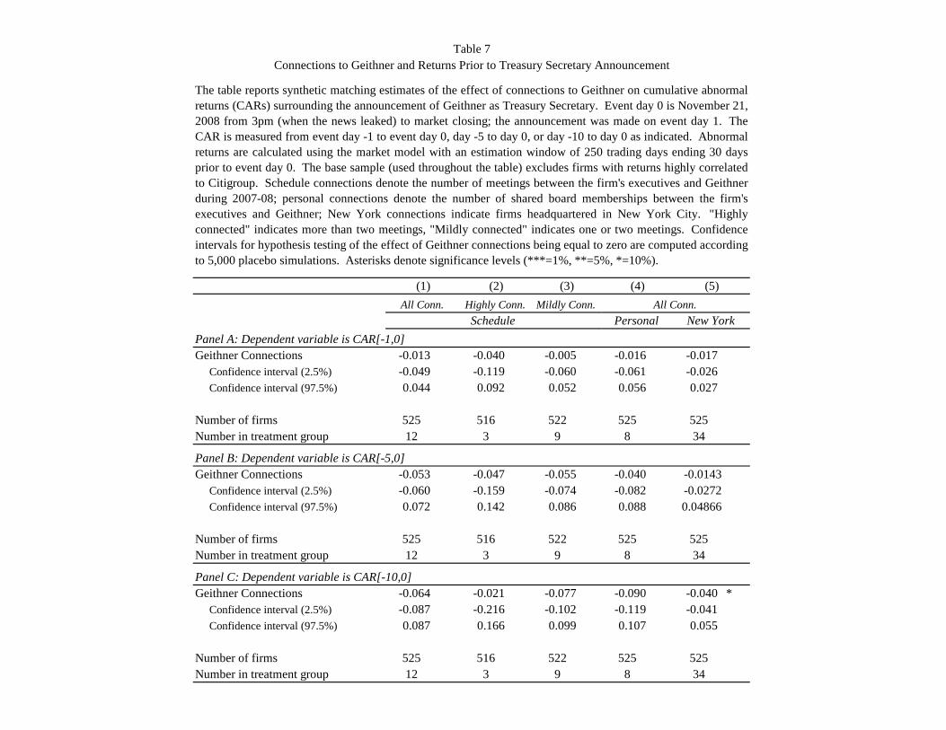
Panel A: Dependent variable is CAR[-1,0]Geithner Connections -0.013 -0.040 -0.005 -0.016 -0.017 Confidence interval (2.5%) -0.049 -0.119 -0.060 -0.061 -0.026 Confidence interval (97.5%) 0.044 0.092 0.052 0.056 0.027

Number of firms 525 516 522 525 525Number in treatment group 12 3 9 8 34

Panel B: Dependent variable is CAR[-5,0]Geithner Connections -0.053 -0.047 -0.055 -0.040 -0.0143 Confidence interval (2.5%) -0.060 -0.159 -0.074 -0.082 -0.0272 Confidence interval (97.5%) 0.072 0.142 0.086 0.088 0.04866

Number of firms 525 516 522 525 525Number in treatment group 12 3 9 8 34

Panel C: Dependent variable is CAR[-10,0]Geithner Connections -0.064 -0.021 -0.077 -0.090 -0.040 * Confidence interval (2.5%) -0.087 -0.216 -0.102 -0.119 -0.041 Confidence interval (97.5%) 0.087 0.166 0.099 0.107 0.055

Number of firms 525 516 522 525 525Number in treatment group 12 3 9 8 34

Table 7Connections to Geithner and Returns Prior to Treasury Secretary Announcement

The table reports synthetic matching estimates of the effect of connections to Geithner on cumulative abnormalreturns (CARs) surrounding the announcement of Geithner as Treasury Secretary. Event day 0 is November 21,2008 from 3pm (when the news leaked) to market closing; the announcement was made on event day 1. TheCAR is measured from event day -1 to event day 0, day -5 to day 0, or day -10 to day 0 as indicated. Abnormalreturns are calculated using the market model with an estimation window of 250 trading days ending 30 daysprior to event day 0. The base sample (used throughout the table) excludes firms with returns highly correlatedto Citigroup. Schedule connections denote the number of meetings between the firm's executives and Geithnerduring 2007-08; personal connections denote the number of shared board memberships between the firm'sexecutives and Geithner; New York connections indicate firms headquartered in New York City. "Highlyconnected" indicates more than two meetings, "Mildly connected" indicates one or two meetings. Confidenceintervals for hypothesis testing of the effect of Geithner connections being equal to zero are computed accordingto 5,000 placebo simulations. Asterisks denote significance levels (***=1%, **=5%, *=10%).

(1) (2) (3) (4) (5)

Schedule Personal New YorkAll Conn. Highly Conn. Mildly Conn. All Conn.

Panel A: OLS estimates

Geithner Connections -0.014 *** -0.035 *** -0.113 ** -0.010 ** -0.019 ** -0.072 -0.011 -0.030 -0.202 -0.010 -0.019 -0.176(0.002) (0.007) (0.044) (0.005) (0.010) (0.049) (0.007) (0.028) (0.150) (0.022) (0.038) (0.164)

Number of firms 27 27 27 26 26 26 27 27 27 26 26 26R-squared 0.941 0.795 0.615 0.772 0.834 0.748 0.671 0.639 0.726 0.479 0.493 0.674

Panel B: Synthetic matching estimates

Geithner Connections -0.087 *** -0.047 *** -0.119 *** -0.026 *** -0.024 *** -0.044 *** -0.042 -0.092 *** -0.203 *** 0.018 -0.071 *** -0.150 *** Confidence interval (2.5%) -0.003 0.000 -0.005 -0.004 0.000 -0.006 -0.067 -0.019 -0.068 -0.072 -0.034 -0.072 Confidence interval (97.5%) 0.003 0.001 0.008 0.005 0.001 0.011 0.040 0.000 0.055 0.054 0.006 0.072

Number of firms 27 27 27 26 26 26 27 27 27 26 26 26Number in treatment group 7 11 6 6 10 5 7 11 6 6 10 5

Dependent variable is % change in CDS spread [1] Dependent variable is % change in CDS spread [1,10]

Citigroup included Citigroup excludedSchedule Personal New York Schedule

Citigroup included Citigroup excludedPersonal New YorkSchedule Personal New York Schedule Personal New York

(1) (2) (3) (4)

The table reports estimates of the effect of connections to Geithner on CDS spreads surrounding the announcement of Geithner as Treasury Secretary. Panel A reports OLS estimates and Panel B reports syntheticmatching estimates. Event day 0 is November 21, 2008 from 3pm (when the news leaked) to market closing; due to a lack of liquidity and intraday quotes, the changes are measured from day 1, when the announcementwas made. The % change in CDS spread is measured as day 1 only, or from day 1 to day 10, as indicated. Schedule connections denote the number of meetings between the firm's executives and Geithner during 2007-08; personal connections denote the number of shared board memberships between the firm's executives and Geithner; New York connections indicate firms headquartered in New York City. In Panel A, controlvariables (not reported) include cubics in size (log of total assets), profitability (return on equity), and leverage (total debt to total capital) as of 2008; robust standard errors, adjusted for pre-event correlations betweenfirms, are below coefficients in parentheses. In Panel B, the matching window is the 100 days ending 30 days prior to event day 0; confidence intervals for hypothesis testing of the effect of Geithner connections beingequal to zero are computed according to 5,000 placebo simulations. Asterisks denote significance levels (***=1%, **=5%, *=10%).

(5) (6)

Dependent variable is % change in CDS spread [1] Dependent variable is % change in CDS spread [1,10]

Table 8Connections to Geithner and Reactions to Treasury Secretary Announcement, CDS Spreads

(7) (8) (9) (10) (11) (12)

Citigroup included Citigroup excluded Citigroup included Citigroup excludedSchedule Personal New York Schedule Personal New York Schedule Personal New York Schedule Personal New York

Geithner Connections 0.020 *** 0.023 ** 0.017 * -0.035 *** -0.063 *** -0.070 ***(0.005) (0.010) (0.010) (0.007) (0.015) (0.014)

Summers Connections 0.011 -0.024(0.016) (0.034)

Corzine Connections 0.020 0.089 **(0.015) (0.033)

Volcker Connections -0.018 0.052 **(0.019) (0.021)

Bair Connections -0.022(0.038)

Other Candidates Combined 0.002 0.028 ***(0.007) (0.010)

Number of firms 582 582 582 27 27 27R-squared 0.048 0.049 0.048 0.795 0.941 0.880

(3) (4) (5) (6)Dep. variable is % change in CDS spread [1]Dependent variable is CAR [0,1]

Table 9Connections to Other Treasury Secretary Candidates and Reactions to Treasury Secretary Announcement

The table reports coefficient estimates of OLS regressions of cumulative abnormal stock returns (CARs) and percent changes in CDS spreadssurrounding the announcement of Geithner as Treasury Secretary on measures of connections to Treasury Secretary candidates. Event day 0is November 21, 2008 from 3pm (when the news leaked) to market closing; the announcement was made on event day 1. In Columns 1 to 3,the CAR is measured from day 0 to day 1, and in Columns 4 to 6, the percent change in CDS spreads is measured for day 1. Abnormal stockreturns are calculated using the market model with an estimation window of 250 trading days ending 30 days prior to event day 0. Estimatesfor the full sample (excluding Citigroup in CAR results) are reported. Connections denote the number of shared board memberships betweenthe firm's executives and the candidate. Control variables (not reported) include cubics in size (log of total assets), profitability (return onequity), and leverage (total debt to total capital) as of 2008. Robust standard errors, adjusted for pre-event correlations between firms, arebelow coefficients in parentheses. Asterisks denote significance levels (***=1%, **=5%, *=10%).

(1) (2)

ONLINE APPENDIX: ADDITIONAL TABLES (NOT FOR PUBLICATION)

Firm OccurrencesBase

Sample CAR [0,10] Total Assets ($Bn) Firm CAR [0,10] Total Assets ($Bn)JP MORGAN CHASE & CO. 14 N 0.186 2,175.00 WELLS FARGO & CO 0.124 1,310.00CITIGROUP INCO. 34 N 0.743 1,938.00 FREDDIE MAC 0.659 835.60BANK OF AMERICA CORP. 4 N 0.168 1,818.00 US BANCORP 0.078 265.90FANNIE MAE 1 N 1.008 908.50 SUNTRUST BANKS INCO. 0.200 189.10THE GOLDMAN SACHS GPIN. 10 N 0.192 876.20 SLM CORP. 0.064 168.80MORGAN STANLEY 9 N 0.224 658.80 CAPITAL ONE FINL.CORP. -0.053 165.90PNC FINL.SVS.GP.INCO. 3 N 0.044 291.10 BB&T CORP. -0.131 152.00BANK OF NY.MELLON CORP. 7 Y -0.095 237.50 REGIONS FINL.CORP. -0.206 146.20STATE STREET CORP. 1 Y 0.091 173.60 FIFTH THIRD BANCORP -0.232 119.50AMERICAN EXPRESS CO. 2 N 0.029 122.60 KEYCORP 0.062 104.50NORTHERN TRUST CORP. 1 Y 0.117 82.05 AMERIPRISE FINL.INCO. 0.297 94.67CME GROUP INCO. 2 Y 0.010 48.16 CIT GROUP INCO. 0.500 80.45NY.CMTY.BANC.INCO. 2 N -0.078 32.33 COMERICA INCO. 0.037 67.55ASTORIA FINL.CORP. 2 N -0.132 21.98 M&T BK.CORP. -0.045 65.82BLACKROCK INCO. 13 Y 0.082 19.91 MARSHALL & ILSLEY CORP. -0.300 62.34NYSE EURONEXT 2 N 0.089 13.28 ZIONS BANCORPORATION -0.255 54.61THE NASDAQ OMX GP.INCO. 2 Y 0.212 12.05 HUNTINGTON BCSH.INCO. -0.073 54.35THE BLACKSTONE GROUP LP. 6 Y 0.345 8.41 HUDSON CITY BANC.INCO. -0.231 54.09PROVIDENT FINL.SVS.INCO. 2 Y -0.145 6.51 CHARLES SCHWAB CORP. -0.141 51.17LAZARD LTD. 1 Y 0.126 2.79 MF GLOBAL LTD. -0.180 49.18MOODY'S CORP. 2 N 0.114 1.55 E*TRADE FINANCIAL CORP. 0.051 47.50OCH-ZIFF CAP.MAN.GP.LLC. 1 N 0.107 1.02 DISCOVER FINANCIAL SVS. 0.122 39.20BEACON FED.BANC.INCORP. 1 Y 0.039 1.02 POPULAR INCO. -0.194 38.53FEDERATED INVRS.INCO. 1 Y 0.065 0.85 SYNOVUS FINL.CORP. -0.031 35.62EVERCORE PARTNERS INCO. 1 Y 0.485 0.68 FIRST HORIZON NAT. CORP. -0.124 31.02

Firm ConnectionsBase

Sample CAR [0,10] Total Assets ($Bn) Firm CAR [0,10] Total Assets ($Bn)JP MORGAN CHASE & CO. 5 N 0.186 2,175.00 FREDDIE MAC 0.659 835.60CITIGROUP INCO. 9 N 0.743 1,938.00 US BANCORP 0.078 265.90BANK OF AMERICA CORP. 1 N 0.168 1,818.00 BANK OF NY.MELLON CORP. -0.095 237.50WELLS FARGO & CO 1 N 0.124 1,310.00 SUNTRUST BANKS INCO. 0.200 189.10FANNIE MAE 1 N 1.008 908.50 STATE STREET CORP. 0.091 173.60THE GOLDMAN SACHS GPIN. 8 N 0.192 876.20 SLM CORP. 0.064 168.80MORGAN STANLEY 3 N 0.224 658.80 BB&T CORP. -0.131 152.00PNC FINL.SVS.GP.INCO. 1 N 0.044 291.10 REGIONS FINL.CORP. -0.206 146.20CAPITAL ONE FINL.CORP. 1 N -0.053 165.90 FIFTH THIRD BANCORP -0.232 119.50AMERICAN EXPRESS CO. 1 N 0.029 122.60 KEYCORP 0.062 104.50CIT GROUP INCO. 2 Y 0.500 80.45 AMERIPRISE FINL.INCO. 0.297 94.67M&T BK.CORP. 1 N -0.045 65.82 NORTHERN TRUST CORP. 0.117 82.05POPULAR INCO. 1 Y -0.194 38.53 COMERICA INCO. 0.037 67.55BLACKROCK INCO. 2 Y 0.082 19.91 MARSHALL & ILSLEY CORP. -0.300 62.34NYSE EURONEXT 1 N 0.089 13.28 ZIONS BANCORPORATION -0.255 54.61THE NASDAQ OMX GP.INCO. 1 Y 0.212 12.05 HUNTINGTON BCSH.INCO. -0.073 54.35FRANKLIN RESOURCES INCO. 1 N 0.046 9.18 HUDSON CITY BANC.INCO. -0.231 54.09THE BLACKSTONE GROUP LP. 4 Y 0.345 8.41 CHARLES SCHWAB CORP. -0.141 51.17FORTRESS INV.GP.LLC. 1 Y -0.131 1.17 MF GLOBAL LTD. -0.180 49.18CARVER BANCORP INCO. 1 Y -0.116 0.79 CME GROUP INCO. 0.010 48.16GAMCO INVESTORS INCO. 1 Y -0.147 0.67 E*TRADE FINANCIAL CORP. 0.051 47.50

Panel B: Personal ConnectionsPersonal Connection to Geithner No Personal Connection (21 Largest)

Appendix Table A1Comparison of Geithner-Connected Firms to Non-Connected Firms

The table compares firms with identifiable connections to Geithner to those with no connections. Schedule connections (Panel A) denote the number ofmeetings between the firm's executives and Geithner during 2007-08; personal connections (Panel B) denote the number of shared board membershipsbetween the firm's executives and Geithner. "Base Sample" indicates whether the firm is included in the base sample (by virtue of not being highlycorrelated to Citigroup). CAR [0,10] is the cumulative abnormal return for the firm surrounding the announcement of Geithner as Treasury Secretary.Total assets are for the year 2008 from Worldscope.

Panel A: Schedule ConnectionsOn Geithner's Schedule Not on Geithner's Schedule (25 Largest)

Firm Connected Person Position with Firm Connection to GeithnerGeithner's Position with Connection

Connected Person's Position with Connection

American Express Kenneth I. Chenault chairman & CEO National Academy Foundation director directorAmerican Express Kenneth I. Chenault chairman & CEO Partnership for New York City board member vice chairBank of America Patricia E. Mitchell director Council on Foreign Relations member memberBlackRock James E. Rohr director RAND Corporation trustee trusteeBlackRock John A. Thain director Unofficial Adviser to Geithner NA NABlackstone Group J. Tomilson Hill vice chairman Council on Foreign Relations member directorBlackstone Group Paul H. O'Neill special adviser RAND Corporation trustee trusteeBlackstone Group Peter G. Peterson chairman and co-founder Unofficial Adviser to Geithner NA NABlackstone Group Richard E. Salomon adv. board chair, alt. asset mgt. Council on Foreign Relations member vice chairmanCapital One Patrick W. Gross director Council on Foreign Relations member memberCarver Bancorp Deborah C. Wright chairman & president & CEO Partnership for New York City board member directorCIT Group Jeffrey M. Peek chairman & CEO Partnership for New York City board member directorCIT Group Seymour Sternberg director Council on Foreign Relations member memberCIT Group Seymour Sternberg director Partnership for New York City board member directorCitigroup Alain J.P. Belda director Partnership for New York City board member directorCitigroup C. Michael Armstrong director Council on Foreign Relations member memberCitigroup Judith Rodin director Council on Foreign Relations member memberCitigroup Kenneth T. Derr director Council on Foreign Relations member memberCitigroup Michael B.G. Froman managing director Council on Foreign Relations member memberCitigroup Pamela P. Flaherty director, corporate citizenship Council on Foreign Relations member memberCitigroup Richard D. Parsons chairman Partnership for New York City board member chair emeritus, directorCitigroup Robert E. Rubin director Geithner is Protégé of Rubin NA NACitigroup Roberto H. Ramirez director Federal Reserve Bank of New York president int'l advisory boardFannie Mae Herbert M. Allison Jr. President & CEO Economic Club of New York trustee trusteeFannie Mae Herbert M. Allison Jr. President & CEO Partnership for New York City board member directorFortress Inv. Group Richard N. Haass director Council on Foreign Relations member presidentFranklin Resources Anne M. Tatlock director Council on Foreign Relations member memberGAMCO Investors Eugene R. McGrath director Economic Club of New York trustee trusteeGoldman Sachs Ashton B. Carter consultant Council on Foreign Relations member memberGoldman Sachs E. Gerald Corrigan managing director Unofficial Adviser to Geithner NA NAGoldman Sachs James A. Johnson director Council on Foreign Relations member memberGoldman Sachs John C. Whitehead foundation chairman International Rescue Committee trustee trusteeGoldman Sachs Lloyd C. Blankfein chairman & CEO Partnership for New York City board member directorGoldman Sachs Robert D. Hormats vice chairman, GS International Economic Club of New York trustee trustee, vice chairGoldman Sachs Ruth J. Simmons director Council on Foreign Relations member memberGoldman Sachs Stephen Friedman director Council on Foreign Relations member directorGoldman Sachs Stephen Friedman director Federal Reserve Bank of New York president chairJPMorgan Chase Andrew D. Crockett executive committee member Group of Thirty member memberJPMorgan Chase Ellen V. Futter director Council on Foreign Relations member memberJPMorgan Chase James Dimon chairman & CEO Federal Reserve Bank of New York president directorJPMorgan Chase James Dimon chairman & CEO Partnership for New York City board member directorJPMorgan Chase Ratan N. Tata international advisory board RAND Corporation trustee trusteeJPMorgan Chase William M. Daley chairman midwest region Council on Foreign Relations member memberM&T Bank Robert G. Wilmers chairman & CEO Council on Foreign Relations member memberMorgan Stanley Frederick B. Whittemore partner & managing director Council on Foreign Relations member trusteeMorgan Stanley John J. Mack chairman & CEO Partnership for New York City board member directorMorgan Stanley Philip Lader senior adviser RAND Corporation trustee trusteeNASDAQ Robert Greifeld president & CEO Partnership for New York City board member directorNYSE Shirley Ann Jackson director Council on Foreign Relations member directorPNC Fin. Services James E. Rohr chairman & CEO RAND Corporation trustee trusteePopular Richard L. Carrion chairman, president, & CEO Federal Reserve Bank of New York president directorWells Fargo Donald B. Rice director RAND Corporation trustee trustee

Appendix Table A2Personal Connections of Timothy Geithner to Financial Firms

The table lists firms to which Timothy Geithner has connections through one or more individuals. The connections are compiled from March 2009 relationship maps onmuckety.com. The connections represent either known connections between Geithner and an individual or potential connections in that Geithner and the individual areassociated with the same organization.

FirmBase

Sample CAR [0,10] Total Assets ($Bn) Firm CAR [0,10] Total Assets ($Bn)JP MORGAN CHASE & CO. N 0.186 2,175.00 BANK OF AMERICA CORP. 0.168 1,818.00CITIGROUP INCO. N 0.743 1,938.00 WELLS FARGO & CO 0.124 1,310.00THE GOLDMAN SACHS GPIN. N 0.192 876.20 FANNIE MAE 1.008 908.50MORGAN STANLEY N 0.224 658.80 FREDDIE MAC 0.659 835.60BANK OF NY.MELLON CORP. Y -0.095 237.50 PNC FINL.SVS.GP.INCO. 0.044 291.10AMERICAN EXPRESS CO. N 0.029 122.60 US BANCORP 0.078 265.90CIT GROUP INCO. Y 0.500 80.45 SUNTRUST BANKS INCO. 0.200 189.10E*TRADE FINANCIAL CORP. Y 0.051 47.50 STATE STREET CORP. 0.091 173.60BLACKROCK INCO. Y 0.082 19.91 SLM CORP. 0.064 168.80JEFFERIES GP.INCO. N 0.071 19.60 CAPITAL ONE FINL.CORP. -0.053 165.90ICAHN ENTERPRISES LP. Y 0.764 18.82 BB&T CORP. -0.131 152.00NYSE EURONEXT N 0.089 13.28 REGIONS FINL.CORP. -0.206 146.20THE NASDAQ OMX GP.INCO. Y 0.212 12.05 FIFTH THIRD BANCORP -0.232 119.50THE BLACKSTONE GROUP LP. Y 0.345 8.41 KEYCORP 0.062 104.50SIGNATURE BK. Y -0.064 7.11 AMERIPRISE FINL.INCO. 0.297 94.67LABRANCHE & CO.INCO. Y 0.127 3.73 NORTHERN TRUST CORP. 0.117 82.05INTERVEST BCSH.CORP. Y -0.259 2.26 COMERICA INCO. 0.037 67.55STERLING BANC. Y -0.137 2.19 M&T BK.CORP. -0.045 65.82FINL.FED.CORP. Y 0.277 1.94 MARSHALL & ILSLEY CORP. -0.300 62.34INV.TECH.GP. Y 0.164 1.68 ZIONS BANCORPORATION -0.255 54.61ALLBERN.HLDG.LP. Y 0.401 1.60 HUNTINGTON BCSH.INCO. -0.073 54.35MOODY'S CORP. Y 0.114 1.55 HUDSON CITY BANC.INCO. -0.231 54.09NAT.FINL.PTNS.CORP. Y 0.989 1.52 CHARLES SCHWAB CORP. -0.141 51.17FORTRESS INV.GP.LLC. Y -0.131 1.17 MF GLOBAL LTD. -0.180 49.18GFI GROUP INCO. Y -0.278 1.09 CME GROUP INCO. 0.010 48.16BGC PARTNERS INCO. Y 0.328 1.07 DISCOVER FINANCIAL SVS. 0.122 39.20OCH-ZIFF CAP.MAN.GP.LLC. Y 0.107 1.02 POPULAR INCO. -0.194 38.53MSCI INCO. Y 0.090 1.02 SYNOVUS FINL.CORP. -0.031 35.62BERKSHIRE BANCORP INCO. Y -0.190 0.91 NY.CMTY.BANC.INCO. -0.078 32.33CARVER BANCORP INCO. Y -0.116 0.79 FIRST HORIZON NAT.CORP. -0.124 31.02BROADPOINT SECS.GP.INCO. Y 0.204 0.69 THE STUDENT LN.CORP. 0.321 28.14EVERCORE PARTNERS INCO. Y 0.485 0.68 INTACT.BCK.GP.INCORP. 0.073 28.00MEDALLION FINL.CORP. Y 0.146 0.65 THE COLO.BANCGROUP INCO. 0.020 25.50KBW INCO. Y -0.382 0.57 ASSOCIATED BANC-CORP -0.056 24.19GLG PARTNERS INCO. Y -0.012 0.49 BOK FINL.CORP. -0.065 22.73DUFF & PHELPS CORP. Y 0.438 0.35 ASTORIA FINL.CORP. -0.132 21.98COHEN & STEERS INCO. Y 0.204 0.28 RAYMOND JAMES FINL.INCO. -0.020 20.62GREENHILL & CO.INCO. Y -0.064 0.23 PEOPLES UTD.FINL.INCO. -0.174 20.17MARKETAXESS HDG.INCO. Y 0.040 0.21 FIRST BANC. -0.093 19.49COWEN GROUP INCORPORATED Y 0.057 0.20 CAPITALSOURCE INCO. 0.135 18.41CMS BANCORP INCO. Y 0.100 0.20 COMMERCE BCSH.INCO. -0.106 17.53PZENA INV.MAN.INCO. Y -0.151 0.06 WEBSTER FINL.CORP. 0.067 17.39EPOCH HOLDING CORP. Y 0.030 0.05 FIRST CTZN.BCSH.INCO. -0.053 16.75RODMAN & RENSHAW CAP.GP. Y 0.217 0.05 TCF FINANCIAL CORP. -0.026 16.74SIEBERT FINANCIAL CORP. Y -0.031 0.04 AMERICREDIT CORP. 0.363 16.23

Appendix Table A3Comparison of New York Firms to Non-New York Firms

The table compares firms in the sample headquartered in New York City with firms in the sample headquartered elsewhere. CAR [0,10] is the cumulativeabnormal return for the firm surrounding the announcement of Geithner as treasury secretary. Total assets are for the year 2008 from Worldscope.

New York Non-New York (Largest 45)

City National Amcore Financial Wilshire Banc. Stewart Info.Svs. Dollar Financial Comm Bancorp Greene County Banc.Fulton Financial Fed.Agri.Mge. First Regl.Banc. Oritani Financial Legacy Bancorp Landmark Bancorp LSB Finl.TD Ameritrade Irwin Finl. Fcstone Group Firstbank Nat.Bankshares Central Jersey Bancorp River Valley BancorpCullen Fo.Bankers First Merchants Ameris Bancorp Centrue Finl. Fox Chase Bancorp Monarch Finl.Hdg. WSB Financial Gp.Ictl.Ex. Pncl.Finl.Ptns. Lakeland Finl. Horizon Financial Eaton Vance Parke Bancorp Summit State BankValley National Bancorp PMI Group Camden Nat. Mutualfirst Finl. Patriot Nat.BanInc Northeast Bancorp Coml.Nat.Finl.Flagstar Bancorp Banner Seacoast Bkg.Fla. Alliance Finl. Washington Banking Co. Pamrapo Ban Patriot Cap.Fdg.Susquehanna Bcsh. 1st Source First Finl. Peapack-Gladstone Finl. Clifton Svg.Banc. Sun American Bancorp Citizens First Sth.Finl.Gp. First Busey Cascade Bancorp PAB Bankshares Peoples Finl. Capital Southwest Pathfinder Banc.UCBH Holdings S & T Bancorp Enter.Finl.Svs. SEI Invs.Co. Unity Bancorp Cmty.Vly.Banc. Liberty Bancorp Bancorpsouth Taylor Cap.Gp. United Wstn.Banc. Mrch.Bcsh. WGNB Cowlitz Bancorporation Rome Bancorp Sterling Finl. Frontier Finl. Viewpoint Financial Gp. Centerstate Bks.of Fla. Riverview Bancorp BCB Bancorp Cheviot Finl.KKR Financial Hdg.Llc Dime Cmty.Bcsh. Mercantile Bk. Sierra Bancorp Cmty.Bk.Shs.of Indna. Alliance Bksh. Glen Burnie BancorpWhitney Holding Benl.Mut.Banc. Farmers Capital Bk. City Bank 1st.Sth.Banc. Vil.Bk.&.Tst.Finl. Firstcity Finl.East Ws.Banc. Westamerica Ban Macatawa Bank Horizon Banc. North Vly.Ban Central Banc. Louisiana Bancorp Wilmington Tst. Flushing Finl. Penn.Com.Banc. Pulaski Financial 1st.Pactrust Banc. Community Partners Banc. Oak Ridge Finl.Svs.Legg Mason Chemical Finl. First Cmty.Bcsh. Ctzn.& Nthn. PVF Capital Pico Hdg. Old Line Bcsh.Wash.Fed. Bancfirst Banctrust Finl.Gp. First Mariner Ban Ames Nat. American River Bksh. MSB Financial Cathay Gen.Bancorp Hanmi Finl. Univest of Penn. Hawthorn Bcsh. K-Fed Bancorp First Fed.Bksh. Ezcorp Firstmerit First Finl.Banc. Kearny Financial First Security Gp. Federated Invrs. Community Ctl.Bk. Somerset Hills Banc.UMB Finl. Renasant Ocwen Finl. The 1st.of Lng.Isl. C&F Finl. Encore Cap.Gp. Sanders Mos.Har.Gp.TFS Financial Heartland Finl.Usa Newbridge Bancorp Colony Bankcorp SI Finl.Gp. The Bank Holdings Monarch Cmty.Banc.Bank of Hawaii Independent Bk. Fnb United First Financial Nw. Nwh.Thrift Bcsh. 1st Cnt.Ban Thomas Weisel Ptns.Gpin.Wintrust Financial Sun Bancorp Center Finl. Piper Jaffray Cos. Bridge Bancorp Hampden Bancorp Amer.Phys.Ser.Gp.Doral Financial Advanta Trico Bcsh. Tennessee Com.Banc. Tradestation Gp. Oneida Finl. Bay National Privatebancorp Midwest Banc Hdg. Peoples Banc. 1st.Marblehead Harleysville Svg.Finl. Southcoast Finl. Atlantic Bancgroup SVB Financial Group Trustco Bk.Ny ESB Finl. Bofi Holding Monroe Ban Colonial Bksh. First Csh.Finl.Svs.Trustmark Ampal-Amer.Isr. Cadence Financial German Amer.Banc. Ctzn.Sth.Bkg. Evans Bancorp Optimumbank Hdg.Pacific Cap.Banc. Bank Mut. Citizens 1st.Banc. Cash Am.Intl. Rainier Pac.Finl.Gp.Inco Chicopee Bancorp Cmty.Shores Bk.Nat.Penn Bcsh. Wsfs Finl. 1st.Defiance Finl. Appalachian Bcsh. First Nat.Bcsh. NB&T Finl.Gp. Kentucky First Fed.Banc.1st.Niag.Finl.Gp. First Ste.Ban Knight Capital Gp. Abington Bancorp Hingham Instn.For Svg. First Key.Finl. 1st.Fed.of Nthn.Mi.Banc.Mgic Investment Integra Bank Finl.Institutions Harrington Ws.Fgp. Herit.Oaks Banc. Magyar Bancorp Bank of Soca.Franklin Resources First Pl.Finl. Amer.West Ban First Cal.Finl.Gp. Marlin Bus.Svs. Norwood Finl. Mayflower Bancorp Prosperity Bcsh. Janus Capital Gp. Smithtown Banc. Enterprise Bancorp Primus Guaranty Ltd. Heritage Financial Group FPB Bancorp MB Finl. Tierone Oppenheimer Hdg. Pac.Merc.Ban 1st.Fed.Bcsh.of Ark.Inco 1st.Cmty.Bk.of Am. Safegd.Scientifics Umpqua Hdg. Sandy Spring Banc. Oceanfirst Finl. Royal Bcsh.of Penn. Amer.Nat.Bksh. PSB Holdings GS Financial Utd.Cmty.Bks. Equifax Parkvale Finl. Princeton Nat.Banc. Community Capital Brooklyn Fed.Banc. Park Bancorp First Midwest Banc. Affiliated Mgrs.Gp.Inc Sthn.Cmty.Finl. Bank of Granite Ohio Valley Banc Elmira Svg.Bk.Fsb Triangle Capital FNB Bank of The Ozarks The Bancorp Bryn Mawr Bank United Panam Finl. Citizens Cmty.Banc. VSB Bancorp NYCorus Bankshares First Finl.Bksh. Northfield Bancorp Credit Accep. Waddell & Reed Finl.Inc Central Va.Bksh. Intersections Newalliance Bcsh. Townebank Fidelity Sthn. HMN Financial Bank of Commerce Hdg. North Ctl.Bcsh. Oh.Legacy Fid.Nat.Financial Columbia Bkg.Sys. Cardinal Finl. LNB BanInc Citizens Co. First State Finl. Nicholas Financial Capitol Fed.Finl. Hampton Roads Bksh. Ste.Banc. Triad Gty. LSB Asta Funding First Bankshares Utd.Bksh. Old Second Banc. Arrow Finl. Columbia Bancorp United Security Bcsh. World Acceptance Ffd Finl.Santander Bancorp Provident Ny.Banc. Porter Bancorp CFS Bancorp Meta Financial Gp. Ameriana Bancorp Main Street Cap.Old Nat.Banc.(Indiana) Wash.Tst.Banc. Capital Bk. Dearborn Banc. Auburn Nat.BanInc Plumas Banc. Commercefirst Banc.Radian Gp. First Finl.Hdg. Cascade Finl. Westfield Finl. Ctl.Vly.Cmty.Banc. Mackinac Financial Bank of MckenneyBstn.Priv.Finl.Hdg. Independent Bk. Summit Finl.Gp. Pacific Cont. TF Financial Adv.Am.Csh.Adv.Cntrs. Carolina Trust BankHancock Holding Co. Community Tst.Banc. Provident Finl.Hdg. Roma Financial Pac.Premier Banc. Wsb Holdings Am.1st.Tax Exem.Invrs.LpNorthwest Banc. Green Bankshares Sy Bancorp Cmwl.Bksh. Premier Finl.Bancorp Inc Scty.Nat.Finl. Osage Bancshares CVB Financial Simmons First Nat. First Utd. First Ctzn.Banc Home Federal Banc. United Bancorp Oh. QC Holdings Moneygram Intl. Mainsource Finl.Gp. TIB Finl. Wainwright Bk.& Tst.Co. Fidelity Ban Sussex Bancorp JMP Group Provident Bksh. Southwest Bancorp QCR Hdg. Bank of Marin Bancorp Resource Am. Intl.Assets Investors Title Co.Provident Finl.Svs. Security Bank First M & F Shore Bcsh. Tidelands Bcsh. Union Bankshares Microfinancial 1st.Cmwl.Finl. Eurobancshares Consumer Prtf.Svs. Eastern Va.Bksh. Peoples Cmty.Banc. Jacksonvl.Banc.Fla. Cougar Biotech.Investors Bancorp Lazard Ltd. Suffolk Banc. CNB Finl. Access National First Cap.Bancorp Arbinet Thexchange Oriental Finl.Gp. SCBT Financial Encore Bancshares First Finl.Ser. Codorus Vly.Banc. Prvt.Cmty.Bcsh. Westwood Hdg.Gp.Mastercard First Bancorp Bnc Bancorp Beacon Fed.Banc.In Tower Finl. Newport Bancorp US Global Invrs.Bankatlantic Banc. T Rowe Price Gp. Metrocorp Bcsh. Center Banc. Sthn.First Bcsh. Sthn.Nat.Banc.of Va.Inco Dia.Hill Inv.Gp.Capitol Banc.Ltd. Va.Com.Bancorp Bankfinancial Essa Bancorp Timberland Banc. Ntheast.Cmty.Banc. Paulson Cap.Iberiabank Southside Bcsh. Mbt Finl. Northrim Bancorp Ocean Shore Co. WVS Finl. Arrowhead Resh.Western Union Co.(The) Cobiz Financial West Ban Atl.Sthn.Finl.Gp. Gamco Investors All.Banc.of (Penn.) Kent Finl.Svs.Glacier Bancorp Berk.Hills Banc. Bank of Florida Atlantic Cst.Fed. Guaranty Fed.Bcsh. Southern Mo.Banc. Community BancorpPenson Worldwide Nara Banc. Compucredit Severn Banc. Bch.First Nat.Bcsh. Abigail Adams Nat.Banc. Bankunited Finl.Harleysville Nat. Great Sthn.Bancorp Banc.Rhode Isl. Middleburg Finl. Prtf.Rec.Assocs. Britton & Koontz Cap. Benjamin Frank.Banc.IncoCentral Pac.Finl. Lakeland Bancorp Rockville Finl. Compass Diversified Hdg. Rurban Finl. Asset Accep.Cap. W Holding Company NBT Bancorp United Cmty.Finl. Yadkin Valley Finl. Optionsxpress Hdg. Community West Bcsh. Broadway Financial Vineyard National Banc.Wesbanco Brookline Bancorp Stifel Finl. Hopfed Bancorp First Clover Leaf Finl. Lake Shore Bancorp Cape Fear Bank Western All.Ban Home Bancshares NASB Finl. Crescent Financial Penns Woods Banc. Wayne Svg.Bcsh. Amer.Cmty.Bcsh.Cmty.Bk.Sy. Union Bankshares Heritage Com. Ameriserv Finl.Inc First Cmty. Carrollton Banc.Anchor Banc.Wi. Newstar Financial Temecula Vly.Banc. Coop.Bankshares Amer.Bancorp of Nj. Jeffersonville BancorpTexas Capital Bcsh. City Co. Eagle Banc. Rep.First Banc.Inco Carolina Bk.Hdg. Calamos Asset Man.SWS Gp. West Coast Bancorp Premier West Bancorp Bridge Cap.Hdg. Utd.Bcsh.Ohio Cal.1st.Nat.BancorpSterling Bcsh. Cap.City Bk.Gp. Preferred Bank Heritage Financial New Century Banc. United Community Bancorp

Appendix Table A4Other Non-New York Firms

The table lists firms in the sample not listed in Appendix Table A4. The firms are listed in descending order of size (total assets).

Panel A: Actual returns, Full sample

Event Day Date Conn. Non-Conn. Conn. Non-Conn. Conn. Non-Conn.0 11/21/2008 0.093 0.047 0.046 *** 0.096 0.047 0.049 *** 0.089 0.046 0.043 ***1 11/24/2008 0.165 0.054 0.111 *** 0.185 0.054 0.131 *** 0.107 0.055 0.052 ***2 11/25/2008 0.032 0.015 0.017 0.047 0.015 0.032 0.033 0.014 0.0193 11/26/2008 0.087 0.042 0.045 ** 0.076 0.043 0.034 0.085 0.040 0.045 ***4 11/28/2008 0.051 0.018 0.033 ** 0.054 0.018 0.036 ** 0.021 0.019 0.0025 12/1/2008 -0.151 -0.083 -0.068 *** -0.165 -0.083 -0.082 *** -0.118 -0.083 -0.034 **6 12/2/2008 0.054 0.046 0.008 0.058 0.046 0.012 0.086 0.043 0.043 ***7 12/3/2008 0.045 0.020 0.024 0.056 0.020 0.036 ** 0.035 0.020 0.0158 12/4/2008 -0.009 -0.014 0.005 -0.003 -0.015 0.011 -0.021 -0.014 -0.0089 12/5/2008 0.060 0.029 0.031 ** 0.056 0.029 0.027 * 0.054 0.028 0.026 **

10 12/8/2008 0.073 0.027 0.046 ** 0.072 0.028 0.045 ** 0.057 0.027 0.030 **0-10 (Cumulative) 0.584 0.197 0.387 *** 0.646 0.197 0.448 *** 0.512 0.189 0.323 ***

Panel B: Cumulative abnormal returns, Full sample

Event Day Date Conn. Non-Conn. Conn. Non-Conn. Conn. Non-Conn.0 11/21/2008 -0.016 -0.015 0.000 -0.025 -0.015 -0.010 -0.007 -0.016 0.0091 11/24/2008 0.046 -0.020 0.066 *** 0.046 -0.020 0.065 *** 0.010 -0.020 0.029 *2 11/25/2008 0.067 -0.011 0.079 *** 0.080 -0.011 0.091 *** 0.033 -0.011 0.045 **3 11/26/2008 0.097 -0.002 0.099 *** 0.093 -0.001 0.094 *** 0.069 -0.003 0.072 ***4 11/28/2008 0.131 0.007 0.124 *** 0.130 0.008 0.121 *** 0.076 0.007 0.069 **5 12/1/2008 0.120 0.005 0.115 *** 0.120 0.005 0.115 *** 0.083 0.003 0.079 ***6 12/2/2008 0.110 0.014 0.096 *** 0.107 0.015 0.092 ** 0.113 0.010 0.103 ***7 12/3/2008 0.112 0.010 0.102 *** 0.116 0.011 0.105 ** 0.111 0.007 0.104 ***8 12/4/2008 0.149 0.022 0.126 *** 0.163 0.023 0.140 *** 0.130 0.019 0.111 ***9 12/5/2008 0.150 0.018 0.132 *** 0.154 0.018 0.135 *** 0.133 0.014 0.119 ***10 12/8/2008 0.161 0.010 0.151 *** 0.157 0.011 0.147 *** 0.136 0.006 0.129 ***

Appendix Table A5Connections to Geithner and Stock Price Reactions to Treasury Secretary Announcement, Full Sample

The table presents stock returns of financial firms around the announcement of Barack Obama's nomination of Timothy Geithner as Treasury Secretary.Event day 0 is November 21, 2008 from 3pm (when the news leaked) to market closing; the announcement was made on event day 1. Abnormal returns arecalculated using the market model with an estimation window of 250 trading days ending 30 days prior to event day 0. Schedule connections indicatemeetings between the firm's executives and Geithner during 2007-08; personal connections indicate shared board memberships between the firm's executivesand Geithner; New York connections indicate firms headquartered in New York City. Asterisks denote significance levels of a two-tailed t-test (***=1%,**=5%, *=10%).

Schedule Connections Personal Connections New York Connections

Difference Difference Difference

Difference Difference Difference

Schedule Connections Personal Connections New York Connections

Conn. Non-Conn. Conn. Non-Conn. Conn. Non-Conn.Geithner Connections (Schedule) 0.046 -0.026 0.072 ** 0.060 0.006 0.054 * 0.064 0.016 0.048

(0.030) (0.033) (0.034)Geithner Connections (Personal) 0.046 0.006 0.039 0.054 -0.002 0.057 0.054 0.015 0.039

(0.033) (0.032) (0.034)Geithner Connections (New York) 0.010 -0.015 0.025 0.010 -0.008 0.018 0.015 -0.014 0.029

(0.022) (0.027) (0.027)

Conn. Non-Conn. Conn. Non-Conn. Conn. Non-Conn.Geithner Connections (Schedule) 0.161 0.021 0.140 ** 0.127 -0.013 0.140 *** 0.131 0.087 0.045

(0.066) (0.052) (0.069)Geithner Connections (Personal) 0.157 0.009 0.149 * 0.115 0.022 0.093 0.115 0.021 0.094

(0.078) (0.068) (0.068)Geithner Connections (New York) 0.136 0.098 0.038 0.139 0.026 0.112 ** 0.140 0.052 0.088 *

(0.059) (0.054) (0.053)

Panel C: Nonparametric matching estimator

PersonalGeithner Connections 0.0047 *** 0.0238 *** 0.0413 *** 0.022 *** 0.054 *** 0.066 ** 0.050 *** 0.098 *** 0.292 ***

(0.0014) (0.0028) (0.0098) (0.005) (0.009) (0.026) (0.010) (0.021) (0.058)

(7)

Dependent variable is CAR [0](Full sample)

(1) (2) (3) (4) (5)

Dependent variable is CAR [0,1](Base sample)

Dependent variable is CAR [0,10](Base sample)

Match on Firm SizePanel B: Propensity-score matched, CAR [0,10]

Schedule Personal New York Schedule New York Schedule

Primary Controls and Others

Personal New York

(9)

Difference Difference Difference

Difference Difference Difference

(8)(6)

Match on Primary Control Variables Primary Controls and Others

Appendix Table A6Cumulative Abnormal Returns of Connected Firms, Matching Estimators

The table reports results from various matching estimators. Panels A and B compare cumulative abnormal returns (CARs) of firms connected to Geithner with cumulative abnormalreturns of non-connected firms matched by propensity score. The CAR is measured from day 0 to day 1 or from day 0 to day 10, as indicated. Matching is done in one of threeways, as indicated: by firm size, by the primary control variables (size, profitability, and leverage), or by the primary control variables plus other control variables (a TARPparticipation dummy, a deposit-taking dummy, and the CAR surrounding the Lehman collapse). Matching is performed as one-to-one matching without replacement. Panel Creports the weighted average estimates computed separately for every covariate cell of regressions of cumulative abnormal returns (CARs) surrounding the announcement ofGeithner as Treasury Secretary on measures of connections to Geithner. Covariates are quartiles of log of total assets, profitability, and leverage, which results in 64 cells. Controlsfor log of total assets, profitability, and leverage are included in each regression. Standard errors are in parentheses, and asterisks denote significance levels (***=1%, **=5%,*=10%).

Panel A: Propensity-score matched, CAR [0,1]Match on Firm Size Match on Primary Control Variables

Control Group (Synthetic Matches) AM

ERIC

AN

EX

PRES

S

AST

OR

IA F

INL.

CO

RP.

BA

NK

OF

AM

ERIC

A

BA

NK

OF

NY

.MEL

LON

BEA

CO

N F

ED.B

AN

C.

BLA

CK

RO

CK

INC

O.

BLA

CK

STO

NE

CIT

IGR

OU

P IN

CO

.

CM

E G

RO

UP

INC

O.

EVER

CO

RE

PAR

TNER

S

FED

ERA

TED

INV

RS.

INC

O.

GO

LDM

AN

SA

CH

S

JP M

OR

GA

N C

HA

SE &

CO

.

LAZA

RD

LTD

.

MO

RG

AN

STA

NLE

Y

NA

SDA

Q O

MX

NO

RTH

ERN

TR

UST

CO

RP.

NY

.CM

TY.B

AN

C.IN

CO

.

NY

SE E

UR

ON

EXT

PNC

FIN

L.SV

S.G

P.IN

CO

.

PRO

VID

ENT

FIN

L.SV

S.

STA

TE S

TREE

T C

OR

P.

Tota

l con

tribu

tion

to w

eigh

ts

1ST.CMWL.FINL.CORP. 0.03 0.031ST.NIAG.FINL.GP.INCO. 0.05 0.18 0.29 0.52ADV.AM.CSH.ADV.CNTRS. 0.13 0.13AFFILIATED MGRS.GP.INC 0.09 0.13 0.04 0.17 0.08 0.09 0.61ALLBERN.HLDG.LP. 0.16 0.08 0.23 0.48AMERIPRISE FINL.INCO. 0.07 0.01 0.15 0.04 0.19 0.12 0.03 0.61ASSOCIATED BANC-CORP 0.01 0.13 0.05 0.18BANK MUT.CORP. 0.07 0.07BANK OF HAWAII CORP. 0.05 0.05BB&T CORP. 0.06 0.06BROOKLINE BANCORP INCO. 0.16 0.16CAPITAL ONE FINL.CORP. 0.24 0.06 0.02 0.04 0.10 0.03 0.03 0.52CAPITOL BANC.LTD. 0.16 0.16CAPITOL FED.FINL. 0.11 0.11CASCADE FINL.CORP. 0.03 0.03CHARLES SCHWAB CORP. 0.04 0.25 0.19 0.12 0.18 0.23 1.00CHICOPEE BANCORP INCO. 0.44 0.44CITY BANK 0.05 0.05CITY NATIONAL CORP. 0.11 0.11 0.05 0.27CMTY.BK.SHS.OF INDNA. 0.14 0.14COMERICA INCO. 0.13 0.13COOP.BANKSHARES INCO. 0.05 0.05CULLEN FO.BANKERS INCO. 0.11 0.06 0.07 0.05 0.07 0.36CVB FINANCIAL CORP. 0.02 0.08 0.10DOLLAR FINANCIAL CORP. 0.01 0.01EATON VANCE CORP. 0.22 0.10 0.06 0.18 0.08 0.64EQUIFAX INCO. 0.23 0.26 0.18 0.67FIFTH THIRD BANCORP 0.18 0.17 0.34FIRST FINL.HDG.INCO. 0.05 0.05FIRST HORIZON NAT.CORP. 0.02 0.02FIRSTMERIT CORP. 0.10 0.06 0.06 0.06 0.09 0.04 0.41FLUSHING FINL.CORP. 0.08 0.08FPB BANCORP INCO. 0.06 0.06FRANKLIN RESOURCES INCO. 0.09 0.10 0.08 0.09 0.10 0.03 0.11 0.14 0.73FULTON FINANCIAL CORP. 0.08 0.08HARLEYSVILLE NAT.CORP. 0.07 0.07HUDSON CITY BANC.INCO. 0.27 0.25 0.51ICTL.EX.INCO. 0.39 0.19 0.19 0.78INDEPENDENT BK.CORP. 0.01 0.01INVESTORS BANCORP INCO. 0.08 0.08JANUS CAPITAL GP.INCO. 0.04 0.08 0.02 0.08 0.03 0.25JEFFERIES GP.INCO. 0.02 0.08 0.07 0.01 0.02 0.03 0.23KEYCORP 0.08 0.12 0.03 0.23LEGG MASON INCO. 0.04 0.14 0.05 0.23M&T BK.CORP. 0.01 0.08 0.10MARKETAXESS HDG.INCO. 0.14 0.18 0.32MARSHALL & ILSLEY CORP. 0.04 0.21 0.10 0.05 0.40MB FINL.INCO. 0.06 0.02 0.08NAT.PENN BCSH.INCO. 0.07 0.07NBT BANCORP INCO. 0.27 0.27NEWALLIANCE BCSH.INCO. 0.04 0.04OPTIONSXPRESS HDG.INCO. 0.27 0.04 0.18 0.20 0.70PEOPLES UTD.FINL.INCO. 0.27 0.21 0.48PIPER JAFFRAY COS. 0.17 0.10 0.05 0.09 0.10 0.15 0.04 0.70PNCL.FINL.PTNS.INCO. 0.18 0.18PROSPERITY BCSH.INCO. 0.03 0.06 0.09RAYMOND JAMES FINL.INCO. 0.10 0.04 0.11 0.01 0.02 0.05 0.33REGIONS FINL.CORP. 0.05 0.13 0.18SEI INVS.CO. 0.25 0.03 0.26 0.14 0.27 0.14 0.21 1.31STIFEL FINL.CORP. 0.11 0.11SUN BANCORP INCO. 0.06 0.06SWS GP.INCO. 0.06 0.06T ROWE PRICE GP.INCO. 0.04 0.07 0.14 0.07 0.06 0.08 0.46TD AMERITRADE HLDG.CORP. 0.08 0.02 0.09 0.07 0.26TRADESTATION GP.INCO. 0.27 0.21 0.49TRICO BCSH. 0.10 0.10TRUSTCO BK.CORP.NY 0.12 0.12TRUSTMARK CORP. 0.04 0.04US BANCORP 0.07 0.14 0.27 0.09 0.02 0.11 0.41 0.04 1.14UTD.BKSH.INCO. 0.21 0.21WADDELL & REED FINL.INC 0.04 0.04 0.05 0.13WEBSTER FINL.CORP. 0.13 0.08 0.21WELLS FARGO & CO 0.30 0.04 0.19 0.05 0.06 0.64WEST COAST BANCORP 0.10 0.10WHITNEY HOLDING CORP. 0.03 0.06 0.07 0.16WILMINGTON TST.CORP. 0.10 0.10WINTRUST FINANCIAL CORP. 0.04 0.04WORLD ACCEPTANCE CORP. 0.12 0.12ZIONS BANCORPORATION 0.11 0.05 0.16Sum of smaller weights not listed 0.06 0.02 0.01 0.01 0.01 0.04 0.02 0.02 0.01 0.03 0.04 0.02 0.28Total weights 1.00 1.00 1.00 1.00 1.00 1.00 1.00 1.00 1.00 1.00 1.00 1.00 1.00 1.00 1.00 1.00 1.00 1.00 1.00 1.00 1.00 1.00

Appendix Table A7Weights for Synthetic Matching

Treatment Group (Connected Firms)

The table presents the weights used for the control group (non-connected) firms in the synthetic matching estimates. The weights presented are for the full sample where the treatment group is defined as firms connected according to the schedule measure of connections, as in Panel A of Table 5. Weights less than 0.005 are not reported in the table.

Firm Connected Person Position with Firm Connection to CandidateCandidates' Position with

ConnectionConnected Person's

Position with Connection

BlackRock Laurence D. Fink chairman & CEO Informal Adviser NA NABlackstone Group Richard E. Salomon adv. board chair, alt. asset mgt. Peterson Institute for International Economics director directorBlackstone Group Peter G. Peterson chairman and co-founder Peterson Institute for International Economics director chairmanCharles Schwab Donald G. Fisher director Teach for America director directorCharles Schwab Paula A. Sneed director Teach for America director directorCitigroup Robert E. Rubin director Summers is Protégé of Rubin NA NACitigroup Richard D. Parsons chairman Obama-Biden economic advisory team member memberCitigroup Judith Rodin director Brookings Institution trustee honorary trusteeCitigroup Anne M. Mulcahy director Obama-Biden economic advisory team member memberGoldman Sachs James A. Johnson director Brookings Institution trustee honorary trusteeGoldman Sachs John C. Whitehead foundation chairman Brookings Institution trustee honorary trusteeGoldman Sachs Richard A. Friedman managing director Mount Sinai Medical Center (New York) trustee trusteeGoldman Sachs Suzanne Nora Johnson senior director Brookings Institution trustee trusteeGoldman Sachs Abby Joseph Cohen senior investment strategist Brookings Institution trustee trusteeIcahn Enterprises Carl C. Icahn owner Mount Sinai Medical Center (New York) trustee trusteeJP Morgan Chase George P. Shultz chairman international council American Corporate Partners adv. council member adv. council memberJP Morgan Chase William M. Daley chairman Midwest division Obama-Biden economic advisory team member memberJP Morgan Chase Ernesto Zedillo int'l advisory board member Peterson Institute for International Economics director directorLazard Vernon E. Jordan Jr. director Brookings Institution trustee honorary trusteeMorgan Stanley Laura D'Andrea Tyson director Brookings Institution trustee trusteeMorgan Stanley Laura D'Andrea Tyson director Obama-Biden economic advisory team member memberMorgan Stanley Hutham S. Olayan director Peterson Institute for International Economics director directorMorgan Stanley Laura D'Andrea Tyson director Peterson Institute for International Economics director directorNASDAQ Glenn H. Hutchins director Brookings Institution trustee trusteeNYSE Shirley Ann Jackson director Brookings Institution trustee trusteeOch-Ziff David Windreich partner Mount Sinai Medical Center (New York) trustee trusteeSallie Mae Barry A. Munitz director Broad Foundations governor governorVISA Suzanne Nora Johnson director Brookings Institution trustee trustee

Blackstone Group Peter G. Peterson chairman & co-founder Concord Coalition director founding presidentBlackstone Group Peter G. Peterson chairman & co-founder Japan Society life director life directorBlackstone Group Peter G. Peterson chairman & co-founder Peterson Institute for International Economics director chairmanBlackstone Group Richard E. Salomon adv. board chair, alt. asset mgt. Peterson Institute for International Economics director directorCapital One Patrick W. Gross director Aspen Institute lifetime trustee trusteeCIT Group James S. McDonald director Japan Society life director directorCitigroup Richard D. Parsons chairman Obama-Biden economic advisory team member memberCitigroup Robert E. Rubin director Concord Coalition director directorCitigroup Anne M. Mulcahy director Obama-Biden economic advisory team member memberGoldman Sachs Stephen Friedman director Aspen Institute lifetime trustee trusteeGoldman Sachs John C. Whitehead foundation chairman Financial Services Volunteer Corps honorary chairman co-founder & chairmanGoldman Sachs John C. Whitehead foundation chairman International House chairman honorary trusteeGoldman Sachs Josef Joffe foundation member Aspen Institute lifetime trustee memberGoldman Sachs E. Gerald Corrigan managing director Group of Thirty chairman of the board memberGoldman Sachs Henry Cornell managing director Japan Society life director directorJPMorgan Chase William M. Daley chairman Midwest division Obama-Biden economic advisory team member memberJPMorgan Chase William H. Gray III director Concord Coalition director directorJPMorgan Chase Andrew D. Crockett executive committee member Group of Thirty chairman of the board memberJPMorgan Chase Ernesto Zedillo int'l advisory board member Peterson Institute for International Economics director directorMoody's Henry A. McKinnell Jr. director Japan Society life director life directorMorgan Stanley Laura D'Andrea Tyson director Obama-Biden economic advisory team member memberMorgan Stanley Hutham S. Olayan director Peterson Institute for International Economics director directorMorgan Stanley Laura D'Andrea Tyson director Peterson Institute for International Economics director directorMorgan Stanley Frederick B. Whittemore partner/managing director Aspen Institute lifetime trustee trusteeNASDAQ Merit E. Janow director Japan Society life director directorNYSE James S. McDonald director Japan Society life director director

NYSE Self senior vice president (former) NA NA NA

Bank of New York Gerald L. Hassell president New York Philharmonic director emeritus directorFannie Mae Philip A. Laskawy chairman New York Philharmonic director emeritus directorGoldman Sachs Self chairman & CEO (former) NA NA NAGoldman Sachs John F. W. Rogers partner & foundation trustee Corzine's former chief of staff NA NALazard Philip A. Laskawy director New York Philharmonic director emeritus directorUS Bancorp Jerry W. Levin director New York Philharmonic director emeritus director

Panel D: Jon Corzine

Appendix Table A8Personal Connections of Other Treasury Secretary Candidates to Financial Firms

The table lists firms to which other Treasury Secretary candidates have connections through one or more individuals. The connections are compiled from March 2009 relationship maps onmuckety.com. The connections represent either known connections between the candidate and an individual or potential connections in that the candidate and the individual are associated withthe same organization.

Panel A: Lawrence Summers

Panel B: Paul Volcker

Panel C: Sheila Bair

Panel A: Actual returns, Base sample

Event Day Date Conn. Non-Conn. Conn. Non-Conn. Conn. Non-Conn.0 1/14/2009 -0.054 -0.029 -0.025 -0.053 -0.029 -0.024 -0.054 -0.028 -0.027 **1 1/15/2009 -0.008 0.000 -0.009 -0.024 0.001 -0.025 0.020 -0.001 0.021 **2 1/16/2009 0.005 -0.002 0.007 -0.011 -0.002 -0.009 -0.002 -0.002 0.0003 1/19/2009 -0.119 -0.061 -0.058 ** -0.070 -0.062 -0.009 -0.076 -0.061 -0.015

0-3 (Cumulative) -0.169 -0.090 -0.079 ** -0.145 -0.091 -0.054 -0.110 -0.090 -0.0204 1/20/2009 0.071 0.039 0.032 0.101 0.038 0.062 ** 0.085 0.036 0.049 ***

Panel B: Cumulative abnormal returns, Base sample

Event Day Date Conn. Non-Conn. Conn. Non-Conn. Conn. Non-Conn.0 1/14/2009 -0.014 -0.006 -0.008 -0.008 -0.006 -0.002 -0.018 -0.006 -0.0121 1/15/2009 -0.024 -0.007 -0.018 -0.034 -0.007 -0.028 0.000 -0.008 0.0082 1/16/2009 -0.029 -0.014 -0.015 -0.056 -0.014 -0.042 -0.010 -0.015 0.0053 1/19/2009 -0.085 -0.039 -0.046 -0.056 -0.040 -0.016 -0.028 -0.041 0.0134 1/20/2009 -0.066 -0.030 -0.037 -0.014 -0.031 0.017 0.009 -0.034 0.043 **

Panel C: Actual returns, Full sample .

Event Day Date Conn. Non-Conn. Conn. Non-Conn. Conn. Non-Conn.0 1/14/2009 -0.058 -0.032 -0.026 ** -0.063 -0.032 -0.031 ** -0.059 -0.031 -0.028 ***1 1/15/2009 -0.026 -0.003 -0.023 * -0.051 -0.003 -0.048 *** 0.007 -0.005 0.0122 1/16/2009 -0.011 -0.003 -0.009 -0.031 -0.002 -0.029 ** -0.006 -0.003 -0.0033 1/19/2009 -0.145 -0.066 -0.078 *** -0.132 -0.067 -0.065 *** -0.091 -0.068 -0.023 *

0-3 (Cumulative) -0.217 -0.101 -0.116 *** -0.243 -0.101 -0.142 *** -0.140 -0.103 -0.037 *4 1/20/2009 0.130 0.043 0.087 *** 0.148 0.043 0.105 *** 0.104 0.042 0.063 ***

Panel D: Cumulative abnormal returns, Full sample

Event Day Date Conn. Non-Conn. Conn. Non-Conn. Conn. Non-Conn.0 1/14/2009 -0.013 -0.007 -0.006 -0.015 -0.007 -0.008 -0.018 -0.006 -0.0121 1/15/2009 -0.041 -0.011 -0.030 * -0.068 -0.010 -0.058 *** -0.013 -0.012 -0.0012 1/16/2009 -0.064 -0.020 -0.044 ** -0.111 -0.018 -0.093 *** -0.028 -0.021 -0.0073 1/19/2009 -0.137 -0.047 -0.091 *** -0.166 -0.046 -0.120 *** -0.055 -0.050 -0.0054 1/20/2009 -0.067 -0.037 -0.031 -0.083 -0.036 -0.047 * -0.004 -0.041 0.037 **

Appendix Table A9Connections to Geithner and Stock Price Reactions to Tax Problems

The table presents stock returns of financial firms around the announcement of Geithner's tax errors and delayed confirmation hearing. Event day 0 is January14, 2009; the tax problems were disclosed by the Senate Finance Committee on January 13, 2009 after market closing. Abnormal returns are calculated usingthe market model with an estimation window of 250 trading days ending 30 days prior to event day 0. The base sample excludes firms with returns highlycorrelated to Citigroup or Bank of America. Schedule connections denote the number of meetings between the firm's executives and Geithner during 2007-08; personal connections denote the number of shared board memberships between the firm's executives and Geithner; New York connections indicate firmsheadquartered in New York City. Asterisks denote significance levels of a two-tailed t-test (***=1%, **=5%, *=10%).

Schedule Connections Personal Connections New York ConnectionsDifference Difference Difference

Schedule Connections Personal Connections New York ConnectionsDifference Difference Difference

Schedule Connections Personal Connections New York Connections

Difference Difference Difference

Difference Difference Difference

Schedule Connections Personal Connections New York Connections

Geithner Connections -0.002 -0.010 0.014 -0.003 *** -0.005 0.016 0.001 0.004 0.026 * -0.001 0.005 0.032 **(0.003) (0.010) (0.011) (0.001) (0.004) (0.010) (0.005) (0.014) (0.015) (0.002) (0.006) (0.014)

Number of firms 515 515 515 583 583 583 515 515 515 583 583 583R-squared 0.058 0.058 0.059 0.116 0.113 0.115 0.113 0.113 0.116 0.209 0.209 0.213

Geithner Connections (Schedule) -0.020 -0.048 -0.014 -0.002 -0.031 * 0.016 -0.051 ** -0.081 -0.044 * -0.056 *** -0.173 *** 0.012 Confidence interval (2.5%) -0.035 -0.108 -0.040 -0.018 -0.035 -0.028 -0.040 -0.126 -0.049 -0.021 -0.046 -0.033 Confidence interval (97.5%) 0.042 0.094 0.050 0.032 0.046 0.040 0.072 0.142 0.078 0.055 0.080 0.066

Number of firms 515 507 513 583 570 574 515 507 513 583 570 574Number in treatment group 10 2 8 22 9 13 10 2 8 22 9 13

Dependent variable is CAR [0,1] Dependent variable is CAR [0,3]Base sample Full sample Base sample Full sample

(12)

Dependent variable is CAR [0,1] Dependent variable is CAR [0,3]

Appendix Table A10Connections to Geithner and Reactions to Tax Problems, OLS and Synthetic Matching Estimates

The table reports estimates of the effect of connections to Geithner on cumulative abnormal returns (CARs) surrounding the announcement of Geithner's tax problems. Panel A reports OLS estimates andPanel B reports synthetic matching estimates. Event day 0 is January 14, 2009; the tax problems were disclosed by the Senate Finance Committee on January 13, 2009 after market closing. In Columns 1 to 6,the CAR is measured from day 0 to day 1, and in Columns 7 to 12, the CAR is measured from day 0 to day 3. Abnormal returns are calculated using the market model with an estimation window of 250trading days ending 30 days prior to event day 0. The base sample excludes firms with returns highly correlated to Citigroup or Bank of America. Schedule connections denote the number of meetingsbetween the firm's executives and Geithner during 2007-08; personal connections denote the number of shared board memberships between the firm's executives and Geithner; New York connections indicatefirms headquartered in New York City. "Highly connected" indicates more than two meetings, "Mildly connected" indicates one or two meetings. In Panel A, control variables (not reported) include cubics insize (log of total assets), profitability (return on equity), and leverage (total debt to total capital) as of 2008; robust standard errors, adjusted for pre-event correlations between firms, are below coefficients inparentheses. In Panel B, the matching window is the 250 days ending 30 days prior to event day 0; confidence intervals for hypothesis testing of the effect of Geithner connections being equal to zero arecomputed according to 5,000 placebo simulations. Asterisks denote significance levels (***=1%, **=5%, *=10%).

(1) (2) (3) (4) (8) (9) (10) (11)(5) (6) (7)

Base sample Full sample Base sample Full sample

Panel A: OLS estimates

Schedule Personal New York New YorkSchedule

Panel B: Synthetic matching estimates

New York Schedule Personal New York PersonalPersonal Schedule

All Conn. Highly Conn. Mildly Conn. All Conn. Highly Conn. Mildly Conn. All Conn. Highly Conn. Mildly Conn. All Conn. Highly Conn. Mildly Conn.