The Value of a Statistical Injury: New Evidence from the ... fileof Zurich under grant no. 53211602...

© Swiss Society of Economics and Statistics 2013, Vol. 149 (1) 57–86

a We thank Olivier Steiger, Rainer Winkelmann and Josef Zweimüller for helpful comments and suggestions and Alois Fässler for providing us with the data as well as helpful guide-lines concerning the handling of the data. Financial support from the Swiss National Sci-ence Foundation under grant no. 100012-103970 (Ruf), the research grant of the University of Zurich under grant no. 53211602 (Kuhn), and the Austrian Science Fund (S 10304-G16: “The Austrian Center for Labor Economics and the Analysis of the Welfare State”) is grate-fully acknowledged.

b Department of Economics, University of Zurich, Mühlebachstrasse 86, CH-8008 Zürich, Switzerland; Swiss Federal Institute for Vocational Education and Training (SFIVET); and IZA. Email: [email protected].

c Suva, Fluhmattstrasse 1, CH-6002 Luzern, Switzerland. Email: [email protected] Compensating wage differentials have also been found, for example, for the risk of unemploy-

ment (Moretti, 2000; Lalive, Ruf, and Zweimüller, 2006a), for shift work (Kostiuk, 1990), and uncertainty with respect to future earnings (Feinberg, 1981). Stern (2004) stud-ies the compensating wage differential for being a scientist.

The Value of a Statistical Injury: New Evidence from the Swiss Labor Marketa

Andreas Kuhnb and Oliver Rufc

JEL-Classification: J17, J28, J31Keywords: compensating wage differentials, value of a statistical injury, risk measurement

1. Introduction

Empirical studies document a remarkable increase in the value of life in the past few decades (Costa and Kahn, 2004) and a more general increase in the value of nonmarket goods like health and longevity (Costa and Kahn, 2003; Murphy and Topel, 2006). One important part of this more general trend in the price of health is workers’ willingness to pay for the prevention of workplace-related acci-dents, both fatal and non-fatal. It is also the compensation for workplace safety which has attracted most interest in the empirical literature, and there is a large number of empirical studies which try to pin down the compensation for acci-dent risks (the surveys by Viscusi and Aldy (2003) and Viscusi (1993) are of special interest here; see also the more recent survey by Ashenfelter (2006)).1 Most empirical studies find a positive compensation for fatal accident risk, often yielding high implicit values of a statistical life. For example, Viscusi and Aldy

58 Kuhn / Ruf

Swiss Journal of Economics and Statistics, 2013, Vol. 149 (1)

2 Most importantly perhaps, some studies rely not on direct measures of risk (i.e. number of accidents), but base their analyses on tradeoffs outside the labor market, e.g. on the tradeoff between traffic accidents and the price of automobiles (Dreyfus and Viscusi, 1995) or fatali-ties related to bicycle accidents and the prize of bicycle helmets (Jenkins, Owens, and Wig-gins, 2001). Other studies have used subjective assessments of risk, as for example Viscusi and O’Connor (1984), and Viscusi and Hersch (2001).

3 See Table 5(a) and Table 5(b) in Viscusi and Aldy (2003) for an overview of the relevant lit-erature and the corresponding estimates of the value of a statistical injury.

(2003) report that half of the studies from the U.S. labor market surveyed in their article give a value of a statistical life within the range of $3.8 to $9.0 million (in prices of 2000), the median estimate being about $7 million. Most studies from outside the U.S. labor market give estimates within the same range. It is difficult to assess the exact reasons for this wide range of estimates, since the studies differ in various ways, for example with respect to the available data and risk measure2 or in the econometric methods applied. The evidence on the compensation for non-fatal accident risk is much less coherent, which is somewhat surprising since most studies that present estimates of such compensation are based on the same data as estimates for the compensation for fatal accident risk. Viscusi and Aldy (2003) report, for both the U.S. as well as other labor markets, a probable range for the value of a statistical injury of about $20,000 to about $70,000 per injury.3 Very similar estimates of the value of injury are reported in Leeth and Ruser (2003). Moreover, they also point out considerable differences between different demographic groups. Relatedly, a recent study by Wei (2007) reports substan-tial wage compensation for job-related illness periods, ranging from 27% up to 140% of annual earnings per prevented illness episode per year.

The key problem from the empirical point of view is the potential sorting of workers into jobs differing in their risk of accidents. Hwang, Reed, and Hub-bard (1992), among others, argue that the problem of main concern are differ-ences in unobservables which in turn relate to the productivity of workers and thus may lead to sorting of workers into jobs with different risks. The sorting of workers in turn is endogenous due to the fact that the income elasticity of the value of a statistical life or injury is positive, i.e. more productive workers sort themselves into less risky jobs by accepting ceteris paribus lower wages. Viscusi and Aldy (2003), for example, report an income elasticity of about 0.5–0.6. On the other hand, though, Shogren and Stamland (2002) argue that the bias in estimating the compensating wage differential could run in the other direction, assuming that workers not only differ in their productivity, but also with respect to their skill in avoiding accidents. Thus, workers in risky jobs could be either more tolerant to risk or more skilled in avoiding risk (or both). Thus they show

The Value of a Statistical Injury 59


4 The study by Garen (1988), for example, tries to correct for the endogeneity of job risk by using a system of simultaneous equations where marital status and the number of dependents are used as instruments for the preference over risk. However, one might argue that both mari-tal status and family size are not very good instruments because they are potentially correlated with risk preferences.

that the estimated risk compensation might actually be upward biased, rather than downward biased. Some studies have tried to approach the problem of endogenous sorting by using instrumental variables (Garen, 1988; DeLeire and Levy, 2004).4 One potentially promising way of dealing with the problem of sort-ing is to rely on panel or, ideally, matched employer-employee data (Woodcock, 2008; Dale-Olsen, 2006). The second important empirical issue concerns the measurement of the risk of an accident. First, as pointed out by Mellow and Sider (1983) for example, typical survey data are more often than not plagued by measurement error, i.e. it seems to be the case that workers often misreport their industry affiliation and/or their exact occupation. Assuming that this kind of measurement error is random, this causes the compensating differential to be biased towards zero (Black and Kniesner, 2003). Second, there clearly is a trade-off of the following form. On the one hand, risk measurements at a low level of aggregation are preferred, as otherwise one might mix workers with very different occupations into the same risk categories, giving rise to aggregation bias (Lalive, 2003). On the other hand though, risk measures at a low aggregation level run into the problem that many cells will have zero risk, at least for shorter periods of time. This is specifically true for fatal accident risk, yet obviously also applies to non-fatal injuries.

Our study presents empirical evidence on the compensation for non-fatal acci-dent risk in Switzerland. Our study has three main features. First, we will exclu-sively focus on non-fatal accidents. This focus reflects the fact that most accidents have non-fatal consequences and thus, from the viewpoint of public health and safety, merit the most attention. We though acknowledge that our focus is also due to data availability well as the empirical approach we take, as we will dis-cuss in more detail below. In the year 2004 (which is the year of our empirical analysis), for example, the Swiss Accident Insurance Fund reports about 246,000 non-fatal accidents related to work, but only 188 fatal accidents. The relative risk of experiencing a non-fatal accident versus a fatal accident in a given year is thus about 1300 times higher. Second, we observe the number of non-fatal accidents not only within entire industries, but also within cells defined by industry × skill-level of the job. This is a tremendous advantage from an empirical point of view,

60 Kuhn / Ruf


since risks at (too) high levels of aggregation mix the risks of very different groups of workers and different willingness to pay for avoiding risk, which might lead to biased estimation of the compensation for risk in the workplace. Moreover, in the case of non-fatal accidents, one might argue that average accident severity varies across skill-levels of the job as well. Third, we capitalize on the availability of longitudinal wage information, which allows us to use simple panel estima-tion methods in order to isolate the firm wage component. We believe that our empirical approach, on the one hand using the number of non-fatal accidents within narrower cells than usually available, and on the other hand combining panel data estimation methods with simple sample stratification, transcends the typical hedonic wage function approach often used in the literature on the sub-ject. Besides, we also complement previous evidence for Switzerland. To the best of our knowledge, there is only a single published study on the compensation of accident risk for Switzerland by Baranzini and Ferro-Luzzi (2001), though focusing on fatal accident risk only.

The main findings of our empirical analysis are the following. First, we find that a simple hedonic wage regression yields a compensation for non-fatal acci-dent risk which is statistically not distinguishable from zero, a result that is in line with some previous empirical studies. The leading explanation for this result (which runs counter to theory) is sorting of workers which differ in their unob-served productivity. Second, moving on to, in a sense, more sophisticated (but, we believe, in this case also more reliable) methods, we find a positive point esti-mate for the compensation of non-fatal accident risk for individuals working in jobs with lowest skill-level (simple and repetitive tasks). Our preferred point esti-mate yields an implicit value of a statistical injury of about 35,000 Swiss francs for this group of workers (which lies well within the range given by studies from the U.S. labor market, as well as from studies outside the U.S.). We find no sig-nificant evidence for compensation of non-fatal accident risk for higher skill-levels of the job. Quite to the contrary, we even find a statistically significant negative coefficient on non-fatal accident risk for workers in jobs with higher skill-levels. While we believe that this result is in line with sorting of workers into jobs with different accident risk based on differences in their unobserved productivity, other mechanisms may be at work as well (note though that it is difficult to explain a negative coefficient on accident risk). However, whatever the mechanism driving this result, it underlines the practical importance of using risk measures at lower levels of aggregation when estimating compensation for non-fatal accident risk.

The remainder of this paper is organized as follows. In section 2, we discuss the two data sources we rely on and the construction of the key variables – along with some descriptive statistics. The empirical analysis is presented and discussed



5 The second important labor market survey is the Swiss Labor Force Survey (SLFS; Schweizeri-sche Arbeitskräfteerhebung (SAKE)). There are two main advantages of using the SWSS over the SLFS: First, the SWSS allows isolating the wage firm fixed effect, which is the part of the observed wage where risk compensation should show up. Second, the SWSS is (as opposed to the SLFS) mailed to employers, and misclassification of occupations and industries should therefore be of minimal order only (the same is arguably true for wages).

in section 3. Specifically, we will discuss three different approaches to identifi-cation and estimation. We start with a simple hedonic wage regression model, where the wage is simply regressed on individual- and firm-specific character-istics. The second approach is based on the idea that we can control for indi-vidual unobserved heterogeneity by an appropriate stratification of the sample. The third approach capitalizes on the longitudinal structure of the wage data. We isolate the wage component that is specific to the firm and then use only this part of the wage to estimate risk compensation. Based on our econometric results, we further present estimates of the value of a statistical injury in Swit-zerland. Section 4 concludes.

2. Data

2.1 Data Sources and Key Measures

Our primary data source is the Swiss Wage Structure Survey (SWSS; Lohnstruk-turerhebung (LSE)), a biannual survey among firms which is administered and made available by the Swiss Federal Statistical Office. The SWSS is one of the largest official surveys in Switzerland focused mainly on employment-relevant information.5 The SWSS is a survey of firms, covering the population of large firms along with a random sample of small firms. We use three different waves of the SWSS (from the years 2000, 2002, and 2004) and we extract individual monthly earnings along with several individual-specific characteristics (see section 2.2 below for details). The SWSS includes average gross monthly wages for full-time employment (i.e. 172 hours per month), including mandatory social secu-rity contributions and extra pay (e.g. pay for night work, 13. monthly wage). The SWSS also includes several socio-demographic characteristics (e.g. age, gender, tenure, educational attainment (highest degree), citizenship) and different firm characteristics (most importantly, the size of the firm along with its geographic location).

Our risk measure corresponds to the number of non-fatal accidents within cells defined over industry (forty different industries on a two-digit level) and

62 Kuhn / Ruf


6 There is no common skill variable in the two data sets, but it is possible to closely map the occupational information (major ISCO codes) from the SAIF on the skill-level of the job avail-able from the SWSS. Additional details are available upon request.

7 Note that there is a fundamental trade-off with respect to the risk measure chosen: On the one hand, risk measures on a highly disaggregated level are preferred, such that we do not pool accident risks of individuals working in very different occupations and jobs. This has been pointed at, for example, by Viscusi (1993, p. 1928) noting that “[t]he main deficiency of industry-based data is that they pertain to industry-wide averages and do not distinguish among the different jobs within that industry [...]”. On the other hand, accidents observed at a very low level of aggregation also give rise to estimation problems, because the number of accidents tends towards zero for most cells if we shrink the size of the risk-relevant cells. That, in fact, is the reason why we decided not to use the information about fatal accidents for this study. Disaggregating the number of fatal accidents over the skill-level of job actually yields far too many cells with zero number of accidents.

skill-level of the job (four different levels). The data have been provided by the Swiss Accident Insurance Fund (SAIF; Schweizerische Unfallversicherungsanstalt (Suva)), which is the most important accident insurance fund in Switzerland. The number of non-fatal accidents within industry × skill-level cells are avail-able for the year 2004. One of the main features of our analysis is that our risk measure rk gives the number of non-fatal accidents per year and per 1,000 workers within a given industry × skill-level cell k (instead of within-industry only).6 Data on the absolute number of non-fatal accidents for the year 2004 is available within cells defined over industry × skill-level of job. Now, because the SAIF does not directly have the number of workers within these cells and because workers are not uniformly distributed over these cells, we also need to know the distribution of workers over these cells in order to compute the risk of a non-fatal accident. To this end, we simply use the distribution of workers in the SWSS (from the year 2004), and then approximate the population distribu-tion of workers by multiplying the number of workers within a given cell with the total number of workers which are covered by the SAIF (about 1.827 millions in the year 2004).7 One main advantage of our data is that measurement error in the risk data and industry-affiliation of workers is arguably of minor signifi-cance (as already mentioned, Mellow and Sider (1983) have pointed out the problem of misclassification of both industry and occupation). This is impor-tant because measurement error in the risk variable tends to bias the compensat-ing wage differential towards zero (measurement error in the dependent variable (i.e. wage) is, of course, also common but of less concern). We are confident that measurement error for both our risk measure and industry-affiliation is of no great importance, since the SWSS does not involve employees but obtains the data from the employer directly (such that misclassification of either industry



and/or occupation is unlikely to occur). For the same reason, we also believe that our wage information is more reliable than the information available in typical survey data (although presumably less reliable than administrative data). Addi-tionally, our risk measure is directly obtained from administrative sources and should thus cover all relevant accidents.

At the same time, however, it is clear that non-fatal accidents vary a lot in their severity and thus also in accruing costs or the duration of absence from work (e.g. Schweizerische Unfallversicherungsanstalt, 2009). It may even be plausible to assume that accidents on average are more severe in lower than in higher job skill-levels, implying that the risk coefficient using accident data on the industry level will be downward biased. At the least, this consideration sup-ports our argument that it may be relevant to use accident risk at the industry×

skill-level cells instead of accident risk at the industry level only.

2.2 Descriptive Statistics

Table 1 shows descriptive statistics for both the overall sample as well as the sample of individuals in jobs of the lowest skill-level (that will be used in the empirical analysis discussed below). In both samples, we only consider workers aged between 16 and 64 (for men) and between 16 and 61 (for women). A second restriction applies to the size of the employer. Because we are estimating wage fixed effects for each firm, we also restrict the sample to workers from firms which have at least ten workers in each of the four job skill-levels in each year. The over-all sample includes more than one million individual workers, the subsample of workers in the lowest skill-level (with respect to the job, not with respect to the educational attainment of the worker) consists of about 300,000 individual work-ers. In both cases, there are about 3,500 different firms (due to the restriction on firms). As we will discuss in-depth in section 3 below, our preferred estimation approach will focus exclusively on workers within a given skill-level as collected in the SWSS, as we believe that such a stratification of the workers yields more reliable estimates of the compensating wage differential.

We begin with describing the overall sample, which is representative of the Swiss labor market as a whole. The typical worker in the Swiss labor market has gross earnings equal to 6,300 Swiss francs a month, is about 40 years old and has about 9.5 years of tenure and is more likely to be a man. The average employer has more than 2,800 workers (reflecting the sampling structure of the SWSS as well as the restriction with respect to the selection of the employers). About two thirds of the workers are married, the other third single. The distribution of workers with respect to educational attainment highlights two important characteristics

64 Kuhn / Ruf


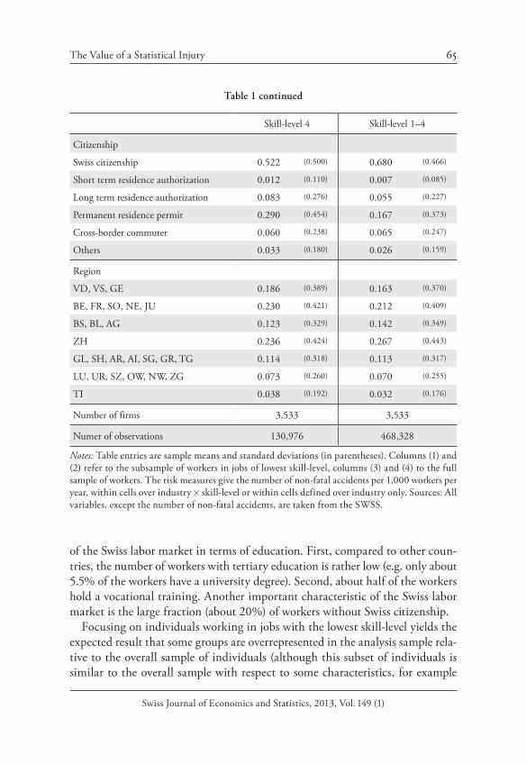
Table 1: Descriptive Statistics

Skill-level 4 Skill-level 1–4

Monthly wage 4,526.625 (1,069.261) 6,371.884 (3,466.716)

ln(monthly wage) 8.392 (0.226) 8.676 (0.381)

Non-fatal accident risk (industry × skill) 45.400 (59.129) 93.007 (150.420)

Non-fatal accident risk (industry) 103.176 (115.139) 93.110 (111.371)

Age 40.189 (11.661) 40.710 (11.143)

Female 0.540 (0.498) 0.421 (0.494)

Tenure 7.633 (8.181) 9.058 (9.121)

Size of the firm 2,714.938 (7,820.838) 3,108.008 (7,890.729)

Management level

Highest/high 0.000 (0.005) 0.024 (0.153)

Medium 0.000 (0.013) 0.057 (0.232)

Low 0.004 (0.064) 0.092 (0.289)

Lowest 0.019 (0.138) 0.081 (0.273)

Without executive function 0.976 (0.152) 0.746 (0.435)

Marital status

Single 0.267 (0.443) 0.317 (0.465)

Married 0.621 (0.485) 0.583 (0.493)

Others 0.112 (0.315) 0.100 (0.301)

Education

University degree 0.003 (0.054) 0.055 (0.228)

College of higher education 0.003 (0.052) 0.048 (0.214)

Higher professional degree 0.006 (0.078) 0.074 (0.261)

Teachers’ certificate 0.001 (0.039) 0.005 (0.068)

High School 0.012 (0.108) 0.020 (0.139)

Finished professional education 0.274 (0.446) 0.505 (0.500)

Firm intern professional education 0.138 (0.344) 0.067 (0.251)

Secondary school 0.480 (0.500) 0.176 (0.381)

Other degree 0.083 (0.277) 0.050 (0.219)



of the Swiss labor market in terms of education. First, compared to other coun-tries, the number of workers with tertiary education is rather low (e.g. only about 5.5% of the workers have a university degree). Second, about half of the workers hold a vocational training. Another important characteristic of the Swiss labor market is the large fraction (about 20%) of workers without Swiss citizenship.

Focusing on individuals working in jobs with the lowest skill-level yields the expected result that some groups are overrepresented in the analysis sample rela-tive to the overall sample of individuals (although this subset of individuals is similar to the overall sample with respect to some characteristics, for example

Skill-level 4 Skill-level 1–4

Citizenship

Swiss citizenship 0.522 (0.500) 0.680 (0.466)

Short term residence authorization 0.012 (0.110) 0.007 (0.085)

Long term residence authorization 0.083 (0.276) 0.055 (0.227)

Permanent residence permit 0.290 (0.454) 0.167 (0.373)

Cross-border commuter 0.060 (0.238) 0.065 (0.247)

Others 0.033 (0.180) 0.026 (0.159)

Region

VD, VS, GE 0.186 (0.389) 0.163 (0.370)

BE, FR, SO, NE, JU 0.230 (0.421) 0.212 (0.409)

BS, BL, AG 0.123 (0.329) 0.142 (0.349)

ZH 0.236 (0.424) 0.267 (0.443)

GL, SH, AR, AI, SG, GR, TG 0.114 (0.318) 0.113 (0.317)

LU, UR, SZ, OW, NW, ZG 0.073 (0.260) 0.070 (0.255)

TI 0.038 (0.192) 0.032 (0.176)

Number of firms 3,533 3,533

Numer of observations 130,976 468,328

Notes: Table entries are sample means and standard deviations (in parentheses). Columns (1) and (2) refer to the subsample of workers in jobs of lowest skill-level, columns (3) and (4) to the full sample of workers. The risk measures give the number of non-fatal accidents per 1,000 workers per year, within cells over industry × skill-level or within cells defined over industry only. Sources: All variables, except the number of non-fatal accidents, are taken from the SWSS.

Table 1 continued

66 Kuhn / Ruf


8 The distribution of workers over the skill-level of jobs looks as follows: About 6% work in the highest level, about 20% in the second-highest level. 46% work in skill-level 3, and the remaining 28% of the workers are in jobs of lowest skill-level.

9 Additional suggestive evidence in favor of this presumption is presented in Figure A.1 in the appendix, showing the distribution of log monthly wages by skill-level of the job. Note how not only the mean, but also the variation of log wages decreases as we move from highest to lowest skill level.

age and size or the geographic location of the employer).8 Here, average monthly earnings are only about 70% of the overall average earnings (about 4,500 Swiss francs per month). Moreover, a worker from skill-level four is more likely to be a woman, more likely to be married and much more likely not to have Swiss cit-izenship, compared with a worker from the overall sample. The most striking difference between the overall sample and the lowest skill-level sample though is the distribution of workers with respect to educational attainment. As Table 1 shows, there are practically no workers with an educational degree above voca-tional training. This, in fact, is a desired result with respect to the empirical approach we take (see section 3 below): Given that education (of course not exclusively) reflects differences in productivity, focusing on workers with simi-lar educational attainment also implies that these workers are more similar with respect to unobserved productivity-relevant characteristics (compared to work-ers from all job skill-levels). We believe that the variance of unobserved produc-tivity is presumably lowest within the group of workers in the lowest skill-level (although this presumption obviously is fundamentally empirically untestable).9

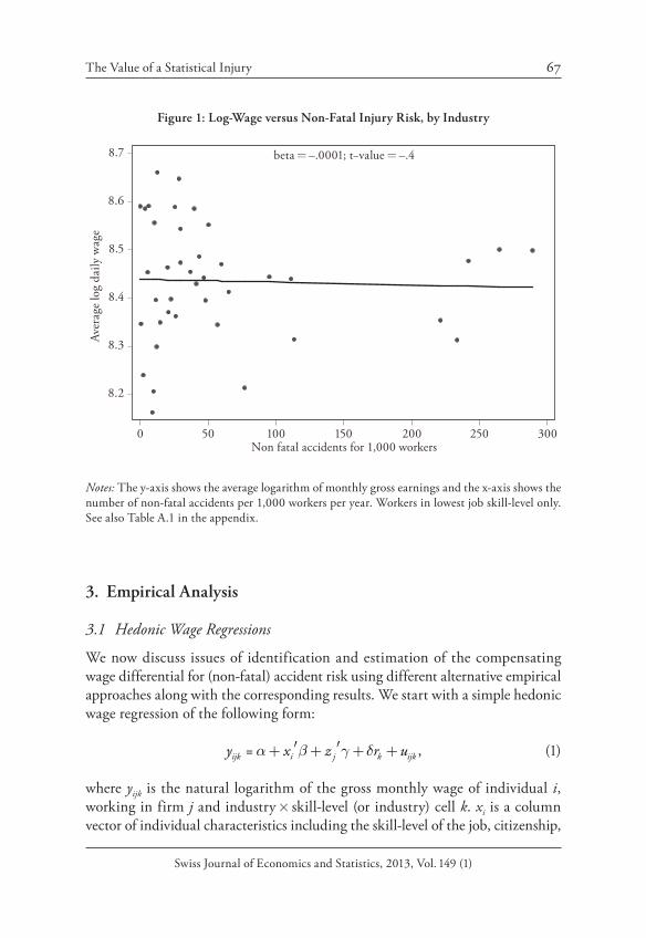
As Table 1 also shows, the typical worker in the year 2004 was faced with the risk of a non-fatal, work-related accident of about 9.3% (i.e. there were 93 acci-dents on average per 1,000 workers). In the sample of workers with lowest skill-level, the average risk was about half (about 45.4 accidents per 1,000 workers). Figure 1 shows a simple scatterplot between the average logarithmic monthly wage and the number of non-fatal accidents for workers from the lowest skill-level jobs at the level of industry × skill-level. The scatterplot shows no relation what-soever between the two variables (if anything, the association goes the “wrong” way), which is underlined by the estimated slope coefficient from a regression of the average log earnings on the number of accidents – yielding essentially a zero point estimate, both in economic and statistical terms (the corresponding t-value is approximately zero). This result is not especially surprising though since aver-age wages within industries clearly may not only reflect differences with respect to accident risks, but also differences in the composition of workers and jobs.



3. Empirical Analysis

3.1 Hedonic Wage Regressions

We now discuss issues of identification and estimation of the compensating wage differential for (non-fatal) accident risk using different alternative empirical approaches along with the corresponding results. We start with a simple hedonic wage regression of the following form:

= ,ijk i j k ijky x z r uα β γ δ′ ′+ + + + (1)

where yijk is the natural logarithm of the gross monthly wage of individual i, working in firm j and industry × skill-level (or industry) cell k. xi is a column vector of individual characteristics including the skill-level of the job, citizenship,

Figure 1: Log-Wage versus Non-Fatal Injury Risk, by Industry

Ave

rage

log

daily

wag

e

0 50 100 150 200 250 300Non fatal accidents for 1,000 workers

beta = –.0001; t−value = –.48.7

8.6

8.5

8.4

8.3

8.2

Notes: The y-axis shows the average logarithm of monthly gross earnings and the x-axis shows the number of non-fatal accidents per 1,000 workers per year. Workers in lowest job skill-level only. See also Table A.1 in the appendix.

68 Kuhn / Ruf


10 Many, if not most, other empirical studies face the same problem of not observing the relevant risk measure over time, as pointed out by Hwang, Reed, and Hubbard (1992, p. 836): “While studies of this sort [i.e. panel studies] represent improvements over standard cross-sectional studies, their applicability is restricted by the availability of longitudinal data sets that include the relevant nonwage job attribute variables. In most cases, this is a binding constraint.”

11 Note that the error term εijk potentially also includes unobserved heterogeneity with respect to the firm (Woodcock, 2008). We will take up this issue below.

educational attainment, age (and its square), tenure (and its square), a gender-dummy, management level and marital status. zj is a column vector of character-istics describing the firm (and thus reflecting the characteristics of the job), and includes the size of the firm (and its square) and the geographical location of the firm. rk is our risk measure, corresponding to the number of non-fatal accidents in industry × skill-level (or industry) cell k per 1,000 workers in the year 2004. uijk is the unobserved error term. The parameter of main interest is δ, which, under appropriate assumptions, corresponds to the compensating wage differential for non-fatal accident risk. As mentioned before, the number of non-fatal accidents is only available for a single point in time, so that we can essentially only run a cross-sectional hedonic wage regression.10 However, we do have a partial panel structure with respect to wages, which we will try to capitalize on later. However, as has been pointed out by several authors (e.g. Hwang, Reed, and Hubbard, 1992), there is good reason to act on the assumption that there is unobserved indi-vidual heterogeneity related to wages (that is, these differences somehow reflect differences in productivity not taken into account for by observed variables) and that “safety” is a normal good (i.e. the demand for “safety” increases as income rises). Thus, workers of high productivity sort themselves into less risky jobs by accepting lower wages ceteris paribus. To stick with the model from equation (1), the hedonic wage regression with unobserved individual heterogeneity made explicit can be written as:

=ijk i j k i ijky x z rα β γ δ θ ε′ ′+ + + + + (2)

where (θ + εijk ) corresponds to the error term uijk from equation (1) whereby now we make the problem of individual heterogeneity explicit (for simplicity, θi is res-caled such that the partial effect of θi on yijk is equal to 1).11 Now, even if we can assume that εijk is mean independent of the regressors, identification of the com-pensating wage differential δ is only achieved if the unobserved effect θi is also mean independent. Whenever there is reason to believe otherwise, parameter δ is not identified (and neither are the other parameters identified, but that is of minor importance for our purposes since we are not per se interested in these parameters).



12 That is, the control function approach yields the same estimates as sample stratification if all parameters would be interacted with the variable on which stratification is based on. However,

As discussed in the introduction, the leading reason for a correlation between θi and the accident risk rk is that θi reflects unobserved productivity, which is obviously related to the wage yijk. If the demand for safety actually increases with income and if we are, at the same time, unable to adequately control for produc-tivity differences, then this could quite plausibly lead to a correlation between θi and rk. That is, more productive workers (i.e. workers with above-average θi ) sort themselves into less-risky jobs by accepting lower wages, which in turn leads to a correlation between the productivity measure θi and the risk measure rk, mean-ing that identification of the risk compensation parameter δ must ultimately fail.

Also note that the key regressor, the accident risk rk, is measured at a higher level of aggregation than the dependent variable and this should to be taken into account when doing statistical inference (Woodcock, 2008). We therefore use robust standard errors, clustered at the same level as the risk measure, i.e. either on the industry level or on the level of industry × skill-level of the job.

3.2 Sample Stratification

A first and straightforward way of dealing with the problem of sorting is to strat-ify the sample in such a way as to minimize the variation in the unobserved error component θi. That is, we run the very same hedonic wage regression as given by equation (1), but only on a narrow(er) subset of individuals. Ideally, this subset consists of individuals presumably as similar as possible with respect to θi. That is, stratification is the simple non-parametric variant of the hedonic wage regression before. However, since most often it is very difficult to control for θi, we think that stratifying the sample is probably a more fruitful approach. Our stratification vari-able of primary interest is the skill-level of the job, which is recorded in the SWSS. Let sij ∈ {1, 2, 3, 4} be the skill-level of individual i working in firm j, where s = 1 (s = 4) corresponds to the highest (lowest) skill-level of a given job. We thus run the same hedonic wage regression as in equation (1), but only on a subset of individu-als within a given skill-level s. Specifically, we will run the following regressions:

= with {1,2,3,4}ijk i j k ijk ijy x z r u s sα β γ δ′ ′+ + + + ≥ ∈ (3)

Note that this approach to estimation is basically the same as the control func-tion approach, the main difference being that stratification allows all parameter estimates to vary between different subsets of the sample12. However, we think

70 Kuhn / Ruf


such a fully interacted regression model is, due to the large number of parameters to be esti-mated, often difficult to interpret.

13 As we will show later, our stratification approach actually reduces the differences between groups of workers with respect to the observed wage (see also appendix Figure A.1 again). For example, in the overall sample the difference in mean monthly earnings between men and women amounts to about 1,700 Swiss francs (about one third relative to the female average). In the subsample of workers within the lowest skill-level, the difference in average earnings amounts to only about 630 Swiss francs (relative to the female average, a bit less than 15%). Although this is only suggestive evidence, we still believe that this is exactly what one would expect if the presumption holds that the variance in θ is lower in the lower skill-levels of jobs.

14 Table A.2 in the appendix sheds additional light on this issue. It shows parameter estimates when estimating the hedonic wage regression separately for each skill-level of the job (instead of pooling different skill-levels as in Table 2). It is immediately evident that the estimated

it plausible that the main advantage of the stratification is that we can minimize variation in θi in this way, which ideally renders a consistent estimate of the com-pensating wage differential δ.13

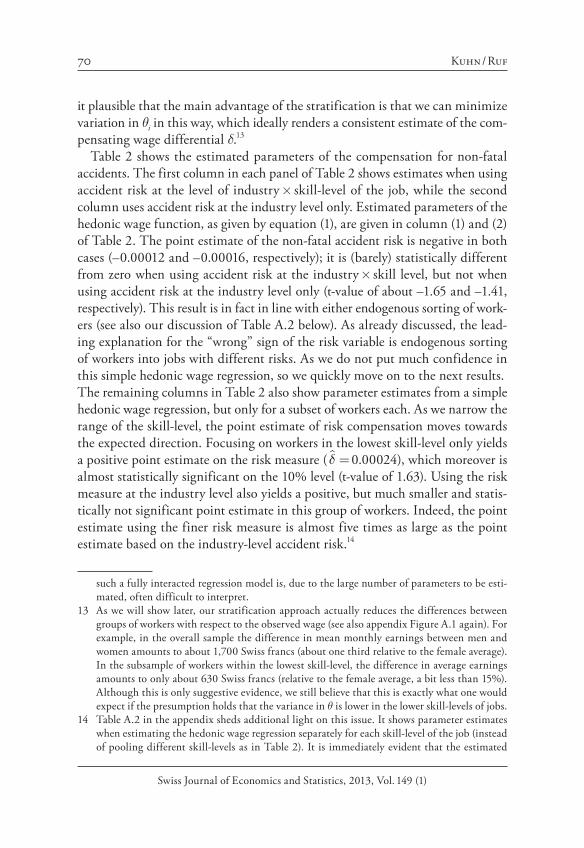
Table 2 shows the estimated parameters of the compensation for non-fatal accidents. The first column in each panel of Table 2 shows estimates when using accident risk at the level of industry × skill-level of the job, while the second column uses accident risk at the industry level only. Estimated parameters of the hedonic wage function, as given by equation (1), are given in column (1) and (2) of Table 2. The point estimate of the non-fatal accident risk is negative in both cases (–0.00012 and –0.00016, respectively); it is (barely) statistically different from zero when using accident risk at the industry × skill level, but not when using accident risk at the industry level only (t-value of about –1.65 and –1.41, respectively). This result is in fact in line with either endogenous sorting of work-ers (see also our discussion of Table A.2 below). As already discussed, the lead-ing explanation for the “wrong” sign of the risk variable is endogenous sorting of workers into jobs with different risks. As we do not put much confidence in this simple hedonic wage regression, so we quickly move on to the next results.The remaining columns in Table 2 also show parameter estimates from a simple hedonic wage regression, but only for a subset of workers each. As we narrow the range of the skill-level, the point estimate of risk compensation moves towards the expected direction. Focusing on workers in the lowest skill-level only yields a positive point estimate on the risk measure (δ"= 0.00024), which moreover is almost statistically significant on the 10% level (t-value of 1.63). Using the risk measure at the industry level also yields a positive, but much smaller and statis-tically not significant point estimate in this group of workers. Indeed, the point estimate using the finer risk measure is almost five times as large as the point estimate based on the industry-level accident risk.14



Tab

le 2

: E

stim

atin

g th

e C

omp

ensa

tion

for

Non

-Fat

al A

ccid

ent

Ris

k U

sin

g th

e O

bse

rved

Wag

e

Dep

ende

nt v

aria

ble

ln(m

onth

ly w

age)

Skill

-lev

el(s

) of

job

1–4

2–4

3–4

4

Mea

n 8.

676

8.63

48.

549

8.39

2

Stan

dard

dev

iati

on

0.38

10.

334

0.28

40.

226

Non

-fat

al a

ccid

ent

risk

(in

dust

ry ×

skill

)–0

.000

12*

(–1.

653)

–0.0

0009

(–1.

402)

–0.0

0009

(–1.

350)

0.00

024

(1.6

26)

Non

-fat

al a

ccid

ent

risk

(in

dust

ry)

–0.0

0016

(–1.

409)

–0.0

0012

(–1.

142)

–0.0

0006

(–0.

554)

0.00

005

(0.4

23)

Add

itio

nal c

ontr

ols

incl

uded

? Ye

sYe

sYe

sYe

sYe

sYe

sYe

sYe

s

Num

ber

of o

bser

vati

ons

468,

328

441,

269

346,

916

130,

976

R2

0.65

40.

654

0.59

30.

593

0.49

30.

491

0.32

10.

318

p-va

lue

(F-s

tati

stic

)0.

000

0.00

00.

000

0.00

00.

000

0.00

00.

000

0.00

0

Roo

t m

ean

squa

red

erro

r0.

224

0.22

40.

213

0.21

30.

202

0.20

30.

186

0.18

6

Not

es: *

, **,

***

den

otes

sta

tist

ical

sig

nifi

canc

e on

the

10%

, 5%

and

1%

leve

l, re

spec

tive

ly. R

obus

t t-

valu

es a

re g

iven

in p

aren

thes

es. S

kill-

leve

l 1 (

4)

corr

espo

nds

to t

he h

ighe

st (

low

est)

ski

ll-le

vel p

ossi

ble.

Add

itio

nal c

ontr

ol v

aria

bles

are

: Age

and

age

squ

ared

, cit

izen

ship

(5

dum

my

vari

able

s), e

du-

cati

onal

att

ain

men

t (8

dum

my

vari

able

s), f

emal

e du

mm

y, g

eogr

aphi

cal r

egio

n (6

dum

my

vari

able

s), j

ob t

enur

e an

d it

s sq

uare

, man

agem

ent

leve

l (4

dum

mie

s),

mar

ital

sta

tus

(2 d

umm

y va

riab

les)

, si

ze o

f th

e fi

rm a

nd i

ts s

quar

e, s

kill-

leve

l of

the

job

(va

ryin

g nu

mbe

r of

dum

mie

s).

Full

regr

essi

on

resu

lts

are

avai

labl

e up

on r

eque

st.

72 Kuhn / Ruf


coefficient on non-fatal accident risk varies substantially across skill-levels. We find a signifi-cant negative coefficient on non-fatal accident risk for individuals working in jobs with higher skill-level (i.e. workers in skill-levels 1 or 2). We still find a negative but insignificant coeffi-cient for skill level 3 and a positive yet also insignificant coefficient for workers in jobs with skill-level 4. While there are several potential explanations of finding a zero coefficient on risk compensation (e.g. sorting of workers into jobs based on unobserved productivity, measure-ment error, differential accident severity across skill-levels), it is hard to explain a negative risk coefficient without reference to workers sorting into jobs of different risk based on unobserved productivity differences. For example, while differences in average accident severity across job skill-levels may lead to attenuation bias in estimating risk compensation, it is difficult to imagine how these differences could lead to a negative coefficient on non-fatal accident risk.

15 Of course, we could capitalize on repeated individual observations using for example the tech-niques proposed by Abowd and Kramarz (1999), but as explained in section 2 we only have temporal information about the employer but not the individual workers.

Also note that the decrease in the R-Squared from about 62% to about 32% reflects the fact that the stratification of the sample absorbs a large part of the varia-tion in the regressors (e.g. educational attainment), which otherwise explain a sig-nificant part of the variation in wages. Nonetheless, the last row of Table 2 shows that the root mean squared error gets smaller as we shrink the sample (0.224 in the overall sample, but only 0.186 in the subsample of workers in the lowest skill-level).

3.3 Wage Decomposition and Firm Wage-Component

Our second approach to identification and estimation is based on quite another idea, which tries to capitalize on the availability of panel data with respect to the firm.15 Still, we can use the additional source of variation in wages stemming from the fact that the SWSS has a longitudinal structure (at least with respect to the firm) such that we can apply simple panel data methods. To start with, let us assume that the observed natural logarithm of the wage yit of individual i in a given year t can (conceptually) be decomposed in a linear model as follows:

=ijt t i j ijty λ φ ψ ε+ + + (4)

Abstracting from time fixed-effects (λt), equation (4) states that individual i’s wage is the sum of an individual wage fixed-effect φi, a firm wage fixed-effect ψj, and a remaining random error component εijt. The critical assumptions in this simple linear fixed effects model are the assumptions about the time invariance of both the individual and the firm fixed effect. However, since we are using panel data spanning only a short time period we believe that these assumptions are innocuous for our application – nonetheless allowing us to resort to the power



16 In this simple conceptual setup λt will pick up any aggregate wage changes (e.g. due to busi-ness cycle fluctuations), while φi and ψj represent the wage component specific to the worker (reflecting ability, for example) and the firm (reflecting accident risk, for example), respectively. The remaining component εijt reflects wage components such as match (and time) specific rents as well as random shocks. In the theory of equalizing wage differentials, firms offer jobs char-acterized by different bundles of wages and non-wage characteristics such as job safety (e.g. Rosen, 1986). Even though ψj still represents different components of compensation specific to the firm (i.e. it may reflect not only differences in accident risk, but also differences in the internal economics of firms, for example), it is the wage component of equation (4) that is clos-est to the concept of equalizing wage differentials (see also Lalive, Ruf, and Zweimüller, 2006b).

of panel data methods. Importantly, note that the theory of compensating wage differentials essentially makes statements about the wage component specific to the employer (i.e. ψj), but not to the individual-specific part nor the random part of the wage.16 If it is possible to consistently estimate the wage firm fixed effect ψj from the available data, we can essentially get rid of individual heterogeneity by simply running a hedonic wage regressing using the estimated wage firm-fixed effect “ jψ instead of the observed wage yijt on our risk measure rk, although we can not directly control for unobserved individual heterogeneity in the hedonic wage regression (because, remember, the risk measure is not observed over time and because there is no person-identifier in the SWSS). Thus, in a first stage, we run a simple regression model using the three consecutive waves of the SWSS:

= with {1,2,3,4}ijt it jt t j ijt ijy x z u s sα β γ λ ψ′ ′+ + + + + ≥ ∈ (5)

Here, as before, xi and zj are vectors of observed individual and firm character-istics, while parameter λt captures aggregate wage shifts over time. The vector xi of observed individual characteristics is important here because we essentially use it to proxy for otherwise unobserved individual heterogeneity. The regres-sion model given by equation (5) is only of interest here because it allows us to estimate the firm wage fixed effects, represented by the vector ψj. Practically, ψj is estimated from the data by including a separate dummy variable for each firm in the sample. In the second stage, we run a regression very similar to the hedonic model from equation (1):

“ = with {1,2,3,4}ijk i j k ijk ijx z r u s sψ α β γ δ′ ′+ + + + ≥ ∈ (6)

where now the dependent variable is the estimated firm wage fixed effect “ ijkψ of individual i working in firm j. Note that the unit of observation is still the indi-vidual worker, although the firm fixed effect obviously does not vary between

74 Kuhn / Ruf


17 The last column in Table A.1 in the appendix shows the estimated firm wage fixed-effect by industry (at the two-digit level, only for the lowest skill-level of jobs).

individuals working in the same firm. This procedure, though, directly applies the right weighting scheme. Again, rk is the non-fatal risk measure in industry × skill-level cell k. Note that we still have to include both vector xi and zj, because the estimated wage firm fixed effect “ jψ is not independent of xi and zj. The main point is that the estimated wage firm fixed effect “ jψ should have been broadly separated from the unobserved individual-specific component φi.

Figure 2: Firm Fixed Effect versus Non-Fatal Injury Risk, by Industry

Wag

e i

rm i

xed

efec

t (s

tand

ardi

zed)

0 50 100 150 200 250 300Non fatal accidents for 1,000 workers

beta = .0025; t−value =1.532

1

0

–1

–2

Notes: The y-axis shows the average of the wage firm fixed effect and the x-axis the number of non-fatal accidents per 1,000 workers per year. Workers in lowest job skill-level only. See also Table A.1 in the appendix.

As shown in Figure 2, a simple scatterplot of the average firm wage fixed-effect (averaged within industries) versus the number of non-fatal accidents shows a clear positive relation between the two variables (as opposed to Figure 1, which showed no relation between the two measures at all).17 A simple regression of



18 Appendix Table A.3 shows estimates for each skill-level of the job separately (see also footnote 3.2).

the average wage firm fixed effect on the number of non-fatal accidents yields an estimated slope coefficient of 0.0025, which almost reaches statistical signifi-cance (t-value of about 1.53).

Results from hedonic wage regressions using the wage firm fixed effect as the dependent variable are shown in Table 3.18 As before, we present results for dif-ferent subsamples defined with respect to the skill-level of the job. It turns out that using the firm fixed effect of the wage instead of the observed wage makes a noticeable difference with respect to the estimated compensation for workplace risk, at least in the subsample of the least skilled workers. Using the accident risk at the more disaggregated level (i.e. at the level of industry × skill-level of the job), the point estimate of the risk parameter more then doubles when using “ jψ instead of yijk as the dependent variable in the regression, yielding a point estimate of 0.00064 (with a significant t-value of about 2.5). In the overall sample and in the other two subsamples, however, using the wage firm fixed effect yields almost the same estimates as when using the observed wage as dependent variable directly. Also, in all three cases, risk estimates turn out to be statistically insignificant. On the other hand, using risk measures at a less aggregated level has the same effect of increasing the point estimate of risk compensation. This is true whether the observed wage or the wage firm fixed effect is used as dependent variable.

3.4 The Value of a Statistical Injury

Given an estimate for the compensation for non-fatal accident risk, we can easily compute the value of a statistical injury (i.e. non-fatal accident). Because all our estimates of the risk parameter are based on semi-logarithmic regressions, the estimated risk coefficient corresponds to the relative wage which 1,000 workers are willing to forego in order to prevent one non-fatal accident (and thus is inde-pendent of the time period chosen). Thus, multiplying the estimated risk param-eter by 1,000 yields the estimated relative value of a statistical injury (VSI). Since our risk measure refers to non-fatal accident per year, we will phrase the VSI in terms of average annual earnings (that is, we multiply VSI additionally with the average annual earnings in the corresponding group of workers).

Table 4 shows estimates for the value of a statistical injury computed from the different estimation methods discussed above (expressed in terms of the average annual earnings in the corresponding sample of workers). The main estimates are based on the point estimate of the risk variable. Lower and upper bounds on

76 Kuhn / Ruf


Tab

le 3

: E

stim

atin

g th

e C

omp

ensa

tion

for

Non

-Fat

al A

ccid

ent

Ris

k U

sin

g th

e W

age

Com

pon

ent

Sp

ecif

ic t

o th

e F

irm

Dep

ende

nt v

aria

ble

Firm

fixe

d ef

fect

Skill

-lev

el(s

) of

job

1–4

2–4

3–4

4

Mea

n –0

.008

–0.0

06–0

.005

0.00

3

Stan

dard

dev

iati

on

0.18

70.

178

0.15

30.

157

Non

fata

l acc

iden

t ri

sk (

indu

stry

× sk

ill)

–0.0

0010

(–1.

406)

–0.0

0008

(–1.

113)

–0.0

0004

(–0.

569)

0.00

064*

*(2

.468

)

Non

-fat

al a

ccid

ent

risk

(in

dust

ry)

–0.0

0014

(–1.

047)

–0.0

0010

(–0.

814)

0.00

000

(0.0

24)

0.00

019*

*(2

.174

)

Add

itio

nal c

ontr

ols

incl

uded

? Ye

sYe

sYe

sYe

sYe

sYe

sYe

sYe

s

Num

ber

of o

bser

vati

ons

468,

328

130,

976

468,

328

130,

976

R2

0.42

50.

425

0.38

60.

386

0.30

40.

303

0.22

00.

183

p-va

lue

(F-s

tati

stic

)0.

000

0.00

00.

000

0.00

00.

000

0.00

00.

000

0.00

0

Roo

t m

ean

squa

red

erro

r0.

142

0.14

20.

139

0.13

90.

128

0.12

80.

139

0.14

2

Not

es: *

, **,

***

den

otes

sta

tist

ical

sig

nifi

canc

e on

the

10%

, 5%

and

1%

leve

l, re

spec

tive

ly. R

obus

t t-

valu

es a

re g

iven

in p

aren

thes

es. S

kill-

leve

l 1 (

4)

corr

espo

nds

to t

he h

ighe

st (

low

est)

ski

ll-le

vel p

ossi

ble.

Add

itio

nal c

ontr

ol v

aria

bles

are

: Age

and

age

squ

ared

, cit

izen

ship

(5

dum

my

vari

able

s), e

du-

cati

onal

att

ain

men

t (8

dum

my

vari

able

s),

fem

ale

dum

my,

geo

grap

hica

l re

gion

(6

dum

my

vari

able

s),

job

tenu

re a

nd i

ts s

quar

e, m

anag

emen

t le

vel

(4 d

umm

ies)

, mar

ital

sta

tus

(2 d

umm

y va

riab

les)

, siz

e of

the

fir

m a

nd it

s sq

uare

, ski

ll-le

vel o

f th

e jo

b (v

aryi

ng n

umbe

r of

dum

mie

s). F

ull r

egre

ssio

n re

sult

s ar

e av

aila

ble

upon

req

uest

.



Table 4: The Estimated Value of a Statistical Injury

Estimated value of a statistical injury (VSI), based on

Yearly earnings Lower bound of δ̂

Point estimate of δ̂

Upper bound of δ̂

A. Accident risk at the level of industry

A.1 Observed wage

Skill-level 1–4 76,463 –28,770 –12,034 4,702

Skill-level 2–4 71,502 –23,327 –8,586 6,156

Skill-level 3–4 64,570 –16,803 –3,702 9,399

Skill level 4 54,320 –9,428 2,592 14,611

A.2 Firm wage fixed effect

Skill-level 1–4 76,463 –31,072 –10,820 9,431

Skill-level 2–4 71,502 –25,445 –7,464 10,518

Skill-level 3–4 64,570 –13,421 163 13,748

Skill-level 4 54,320 1,013 10,284 19,556

B. Accident risk at the level of industry × skill-level of the job

B.1 Observed wage

Skill-level 1–4 76,463 –20,294 –9,284 1,725

Skill-level 2–4 71,502 –15,263 –6,366 2,532

Skill-level 3–4 64,570 –13,678 –5,578 2,522

Skill-level 4 54,320 –2,668 12,986 28,640

B.2 Firm wage fixed effect

Skill-level 1–4 76,463 –19,189 –8,017 3,155

Skill-level 2–4 71,502 –16,838 –5,622 5,594

Skill-level 3–4 64,570 –10,483 –2,358 5,768

Skill-level 4 54,320 7,200 34,952 62,703

Notes: All entries are based on the point estimate δ̂, and the lower and upper bound of the 95% confidence interval of δ̂, respectively.

78 Kuhn / Ruf


the value of a statistical injury are based on the 95% confidence interval of each point estimate of the parameter δ (based on robust standard errors). The simple hedonic wage regression based on the pooled sample actually yields a negative estimate for the value of a statistical injury (per injury per year). Only using the upper bound of the confidence interval yields the expected positive value (although still a small one).

Stratification of the sample by the skill-level of the job yields a higher value of a statistical injury, the narrower the sample. Focusing on workers in the lowest skill-level only gives an estimate of about 2,600 Swiss francs (accident risk at the level of industry only) and about 13,000 Swiss francs (accident risk at the level of industry × skill-level of the job), respectively. However, note that the estimate based on the lower bound of the confidence interval though still gives a nega-tive estimate in both cases.

Finally, for the subsample of less skilled workers and using the wage firm fixed effect gives a significant positive value of a statistical injury (even if we use the lower bound of the corresponding confidence interval). Based on the point esti-mate, we get an estimated value of a statistical injury of about 10,00 and about 35,000 Swiss francs per non-fatal accident averted per year, depending on the risk measure used. This value fits into the range reported by most other empiri-cal studies (see Viscusi and Aldy, 2003, again).

4. Conclusions

We provide empirical estimates of the value of a statistical injury for Switzerland for the year 2004, using non-fatal accident risk within industry × skill-level cells and applying different approaches to identification. Specifically, we stratify the sample by the skill level of the job and we try to statistically isolate the firm-spe-cific wage component, to which the theory of compensating wage differentials conceptually applies most directly.

It turns out that both the risk measure and the empirical method actually make a huge difference with respect to the estimation of risk compensation. Simple hedonic wage regressions actually yield negative or zero compensation for non-fatal accident risk at the workplace. Moving on to methods we believe are more reliable (i.e. consistent) pushes the risk compensation in the “right” direction (i.e. yielding positive compensation for accident risk). Our preferred estimation method, based on using a restricted sample of workers in jobs of lowest skill-level only and using the wage firm fixed effect instead of the observed wage, gives a substantial estimate for the value of a statistical injury of about 35,000 Swiss



francs, which is within the range given by both studies from inside and outside the U.S. labor market. Consistent with existing evidence, individuals’ willing-ness to pay for workplace safety is substantial – reflecting a more general trend in increasing prices in nonmarket goods (Costa and Kahn, 2003).

At the same time, however, we do not find evidence for compensation for non-fatal accident risk for the other groups of workers, i.e. for workers in jobs with higher skill-levels. In fact, results by skill-level of the job even yields a negative coefficient on compensation for non-fatal accident risk for workers with highest skill-levels. While this may cast some doubt on our identification strategy, note that differential sorting of workers based on unobserved productivity differences is in principle compatible with this finding. While it is difficult to find direct evidence on the plausibility of this mechanism, we do find some evidence that appears to be in line with such an hypothesis (smaller variation in overall com-pensation among lower job skill-levels).

Indeed, our analysis – by comparing the magnitude of risk compensation – also sheds some light on the problem of endogenous sorting of workers based on their (unobserved) productivity-relevant characteristics. The more attention we pay to mitigating unobserved productivity differences (i.e. by focusing on nar-rower groups of workers), the larger the estimates for risk compensation we get. This pattern seems to be consistent with the hypothesis that high-productivity workers select into lower-risk jobs by accepting lower wages.

80 Kuhn / Ruf


Appendix: Additional Tables and Figures

Figure A.1: Density Estimates of Log Monthly Wages, by Skill-Level of the Job

7.5 8.0 8.5 9.0 9.5 10.0 10.5ln(monthly wage)

2.0

1.5

1.0

0.5

0.0

Skill-level 1 Skill-level 2

Skill-level 3 Skill-level 4

Notes: The figure shows density estimates of the distribution of log monthly wages, by skill-level of the job (density estimates use the Gaussian kernel). Skill-level 1 (4) corresponds to the highest (lowest) skill-level possible.

Table A.1: Main Variables, by Industry (Lowest Skill-Level Only)

Industry Workers Wage Accidents FFE

Petroleum refining and processing 4692 5,560.13 0.14 0.84

Office material production, data processing 4288 4,302.83 0.59 –0.62

Information technology services 6237 3,933.30 2.39 –0.77

Shipping 55 5,467.47 3.57 0.61

Metal production and processing 7201 4,781.81 5.46 –0.53

Aviation 12 5,496.25 6.22 –0.44

Production of leather goods and shoes 229 3,628.01 8.94 –1.61

Production of clothes and fur goods 270 3,741.27 9.89 –1.92

Insurance industry 2086 5,300.57 10.53 1.46

Production of medical technology 7421 4,523.07 11.55 –0.25

Retail business 19118 4,090.10 12.26 –0.21



Industry Workers Wage Accidents FFE

Tobacco processing 636 5,977.87 12.70 1.44

Production of furniture, jewellery, musical intruments

1743 4,329.91 14.86 –0.26

Machinery, mechanical engineering 5441 4,851.64 20.24 –0.06

Textiles 1350 4,436.00 20.83 –0.74

Automobile industry 1075 4,508.15 22.73 –0.38

Energy- and watersupply 496 5,504.46 25.59 0.59

Traffic support 1502 4,360.78 26.35 –0.53

Credit business 3059 5,833.48 28.60 0.97

Paper and carton production 2153 4,917.06 29.64 –0.21

Credit business and insurance industry 70 5,373.94 29.76 0.92

Printing, publishing and distribution industries 3013 4,833.14 36.99 –0.19

Research and development 202 5,478.94 39.78 1.41

Whole sale 7621 4,683.02 41.36 –0.34

Wood processing 810 4,950.09 43.53 0.14

Transportation 2236 4,724.08 46.89 –0.28

Rubber and plastic production 2657 4,511.65 48.12 –0.61

Mining 80 5,277.08 50.33 0.80

Agriculture 6756 4,310.73 57.05 –0.98

Mining 1217 4,821.76 59.91 –0.25

Health and welfare system 19642 4,582.02 65.31 0.98

Hotel and restaurant industry 9676 3,743.90 76.98 0.02

Real estate 581 4,784.07 95.10 0.74

Information transmission 55 4,707.71 111.04 0.07

Entertainment 814 4,208.07 113.46 –0.43

Education 744 4,394.47 221.19 0.69

Personal services 238 4,318.43 233.62 –0.24

Waste management 95 4,953.19 242.00 0.41

Lobbies, associations, organizations 512 5,067.35 264.88 1.30

Construction 4893 4,965.64 289.03 0.28

Notes: Table entries show sample averages within industries, sorted by accident risk. “Workers” shows the absolute number of observations. “Accidents” shows the number of non-fatal accidents per 1,000 workers. “Wage” shows mean gross monthly earnings. “FFE” denotes the average firm fixed effect, as given by equation (5), and is (in the table) standardized to mean 0 and variance 1.

Table A.1 continued

82 Kuhn / Ruf


Tab

le A

.2:

Est

imat

ing

the

Com

pen

sati

on f

or N

on-F

atal

Acc

iden

t R

isk

Usi

ng

the

Ob

serv

ed W

age,

S

epar

atel

y fo

r E

ach

Sk

ill-

Lev

el o

f th

e Jo

b

Dep

ende

nt v

aria

ble

ln(m

onth

ly w

age)

Skill

-lev

el o

f job

1

23

4

Mea

n 9.

366

8.94

48.

644

8.39

2

Stan

dard

dev

iati

on

0.44

20.

317

0.27

40.

226

Non

-fat

al a

ccid

ent

risk

(in

dust

ry ×

skill

)–0

.000

82**

*(–

4.78

3)–0

.000

35**

(–2.

369)

–0.0

0010

(–1.

475)

0.00

024

(1.6

26)

Non

-fat

al a

ccid

ent

risk

(in

dust

ry)

–0.0

0073

**(–

2.55

1)–0

.000

35**

(–2.

571)

–0.0

0013

(–1.

249)

0.00

005

(0.4

23)

Add

itio

nal c

ontr

ols

incl

uded

? Ye

sYe

sYe

sYe

sYe

sYe

sYe

sYe

s

Num

ber

of o

bser

vati

ons

27,0

5994

,353

215,

940

130,

976

R2

0.45

60.

436

0.44

40.

452

0.42

60.

423

0.32

10.

318

p-va

lue

(F-s

tati

stic

)0.

000

0.00

00.

000

0.00

00.

000

0.00

00.

000

0.00

0

Roo

t m

ean

squa

red

erro

r0.

326

0.33

20.

236

0.23

50.

207

0.20

80.

186

0.18

6

Not

es: *

, **,

***

den

otes

sta

tist

ical

sig

nifi

canc

e on

the

10%

, 5%

and

1%

leve

l, re

spec

tive

ly. R

obus

t t-

valu

es a

re g

iven

in p

aren

thes

es. S

kill-

leve

l 1 (

4)

corr

espo

nds

to t

he h

ighe

st (

low

est)

ski

ll-le

vel p

ossi

ble.

Add

itio

nal c

ontr

ol v

aria

bles

are

: Age

and

age

squ

ared

, cit

izen

ship

(5

dum

my

vari

able

s), e

du-

cati

onal

att

ain

men

t (8

dum

my

vari

able

s), f

emal

e du

mm

y, g

eogr

aphi

cal r

egio

n (6

dum

my

vari

able

s), j

ob t

enur

e an

d it

s sq

uare

, man

agem

ent

leve

l (4

dum

mie

s), m

arit

al s

tatu

s (2

dum

my

vari

able

s), s

ize

of t

he f

irm

and

its

squa

re. F

ull r

egre

ssio

n re

sult

s ar

e av

aila

ble

upon

req

uest

.



Tab

le A

.3:

Est

imat

ing

the

Com

pen

sati

on f

or N

on-F

atal

Acc

iden

t R

isk

Usi

ng

the

Wag

e C

omp

onen

t S

pec

ific

to

the

Fir

m,

Sep

arat

ely

for

Eac

h S

kil

l-L

evel

of

the

Job

Dep

ende

nt v

aria

ble

Firm

fixe

d ef

fect

Skill

-lev

el o

f job

1

23

4

Mea

n –0

.007

2–0

.017

8–0

.010

00.

0027

Stan

dard

dev

iati

on

0.33

60.

282

0.17

30.

157

Non

-fat

al a

ccid

ent

risk

(in

dust

ry ×

skill

) –

0.00

145*

** –

0.00

077*

* –

0.00

009

0.

0006

4**

(–5

.313

) (

–2.4

17)

(–1

.031

)

(2.4

68)

Non

-fat

al a

ccid

ent

risk

(in

dust

ry)

–0.0

0138

***

–0.0

0067

**

–0

.000

15

0.

0001

9**

(–3.

839)

(–2.

341)

(–0.

986)

(2.1

74)

Add

itio

nal c

ontr

ols

incl

uded

? Ye

sYe

sYe

sYe

sYe

sYe

sYe

sYe

s

Num

ber

of o

bser

vati

ons

27,0

5994

,353

215,

940

130,

976

R2

0.

467

0.38

4

0.45

7 0.

481

0.

365

0.36

5

0.22

0 0.

183

p-va

lue

(F-s

tati

stic

)

0.00

0 0.

000

0.

000

0.00

0

0.00

0 0.

000

0.

000

0.00

0

Roo

t m

ean

squa

red

erro

r

0.24

6 0.

264

0.

208

0.20

3

0.13

8 0.

137

0.

139

0.14

2

Not

es: *

, **,

***

den

otes

sta

tist

ical

sig

nifi

canc

e on

the

10%

, 5%

and

1%

leve

l, re

spec

tive

ly. R

obus

t t-

valu

es a

re g

iven

in p

aren

thes

es. S

kill-

leve

l 1 (

4)

corr

espo

nds

to t

he h

ighe

st (

low

est)

ski

ll-le

vel p

ossi

ble.

Add

itio

nal c

ontr

ol v

aria

bles

are

: Age

and

age

squ

ared

, cit

izen

ship

(5

dum

my

vari

able

s), e

du-

cati

onal

att

ain

men

t (8

dum

my

vari

able

s), f

emal

e du

mm

y, g

eogr

aphi

cal r

egio

n (6

dum

my

vari

able

s), j

ob t

enur

e an

d it

s sq

uare

, man

agem

ent

leve

l (4

dum

mie

s), m

arit

al s

tatu

s (2

dum

my

vari

able

s), s

ize

of t

he f

irm

and

its

squa

re. F

ull r

egre

ssio

n re

sult

s ar

e av

aila

ble

upon

req

uest

.

84 Kuhn / Ruf


References

Abowd, John M., and Francis Kramarz (1999), “Econometric Analyses of Linked Employer–Employee Data”, Labour Economics, 6(1), pp. 53–74.

Ashenfelter, Orley (2006), “Measuring the Value of a Statistical Life: Prob-lems and Prospects”, Economic Journal, 116, pp.C10–C23.

Baranzini, Andrea, and Giovanni Ferro-Luzzi (2001), “The Economic Value of Risks to Life and Health: Evidence from the Swiss Labour Market”, Swiss Journal of Economics and Statistics, 137(2), pp. 149–170.

Black, Dan A., and Thomas J. Kniesner (2003), “On the Measurement of Job Risk in Hedonic Wage Models”, Journal of Risk and Uncertainty, 27(3), pp. 205–220.

Costa, Dora L., and Matthew E. Kahn (2003), “The Rising Price of Non-market Goods”, American Economic Review, 93(2), pp. 227–232.

Costa, Dora L., and Matthew E. Kahn (2004), “Changes in the Value of Life, 1940–1980”, Journal of Risk and Uncertainty, 29(2), pp. 159–180.

Dale-Olsen, Harald (2006), “Estimating Workers’ Marginal Willingness to Pay for Safety using Linked Employer-Data”, Economica, 73, pp. 99–127.

DeLeire, Thomas, and Helen Levy (2004), “Worker Sorting and the Risk of Death on the Job”, Journal of Labor Economics, 22(4), pp. 925–954.

Dreyfus, Mark K., and W. Kip Viscusi (1995), “Rates of Time Preference and Consumer Valuations of Automobile Safety and Fuel Efficiency”, Journal of Law & Economics, 38(1), pp. 79–105.

Feinberg, Robert M. (1981), “Earnings-Risk as a Compensating Differential”, Southern Economic Journal, 48(1), pp. 156–163.

Garen, John (1988), “Compensating Wage Differentials and the Endogeneity of Job Riskiness”, Review of Economics and Statistics, 70(1), pp. 9–16.

Hwang, Hae-Shin, W. Robert Reed, and Carlton Hubbard (1992), “Com-pensating Wage Differentials and Unobserved Productivity”, Journal of Politi-cal Economy, 100(4), 835–58.

Jenkins, Robin R., Nicole Owens, and Lanelle Bembenek Wiggins (2001), “Valuing Reduced Risks to Children: The Case of Bicycle Safety Helmets”, Contemporary Economic Policy, 19(4), pp. 397–408.

Kostiuk, Peter F. (1990), “Compensating Differentials for Shift Work”, Jour-nal of Political Economy, 98(5), pp. 1054–1075.

Lalive, Rafael (2003), “Did We Overestimate the Value of Health?”, Journal of Risk and Uncertainty, 27(2), pp. 171–193.



Lalive, Rafael, Oliver Ruf, and Josef Zweimüller (2006a), “Compensat-ing Wage Differentials for Employment Risk: Evidence from Linked Firm-Worker Data”, Mimeo, University of Zurich.

Lalive, Rafael, Oliver Ruf, and Josef Zweimüller (2006b), “Wages and Risks at the Workplace: Evidence from Linked Firm-Worker Data”, Mimeo, University of Zurich.

Leeth, John D., and John Ruser (2003), “Compensating Wage Differentials for Fatal and Nonfatal Injury Risk by Gender and Race”, Journal of Risk and Uncertainty, 27(3), pp. 257–277.

Mellow, Wesley, and Hal Sider (1983), “Accuracy of Response in Labor Market Surveys: Evidence and Implications”, Journal of Labor Economics, 1(4), pp. 331–44.

Moretti, Enrico (2000), “Do Wages Compensate for Risk of Unemployment? Parametric and Semiparametric Evidence from Seasonal Jobs”, Journal of Risk and Uncertainty, 20(1), pp. 45–66.

Moulton, Brent R. (1986), “Random Group Effects and the Precision of Regression Estimates”, Journal of Econometrics, 32(3), pp. 385–397.

Murphy, Kevin M., and Robert H. Topel (2006), “The Value of Health and Longevity”, Journal of Political Economy, 114(5), pp. 871–904.

Rosen, Sherwin (1986), “The Theory of Equalizing Differences”, in Handbook of Labor Economics, O. Ashenfelter and R. Layard, eds., chap. 12, pp. 641–692, Elsevier.

Schweizerische Unfallversicherungsanstalt (2009), „Unfallstatistik UVG 2003–2007. Achtzehnte fünfjährige Beobachtungsperiode der Suva und vierte fünfjährige Beobachtungsperiode aller UVG-Versicherer“, Luzern, Schweiz-erische Unfallversicherungsanstalt (Suva).

Shogren, Jason F., and Tommy Stamland (2002), “Skill and the Value of Life”, Journal of Political Economy, 110(5), pp. 1168–1197.

Stern, Scott (2004), “Do Scientists Pay to Be Scientists?”, Management Sci-ence, 50(6), pp. 835–853.

Viscusi, W. Kip (1993), “The Value of Risks to Life and Health”, Journal of Eco-nomic Literature, 31(4), pp. 1912–1946.

Viscusi, W. Kip, and Joseph E. Aldy (2003), “The Value of a Statistical Life: A Critical Review of Market Estimates throughout the World”, Journal of Risk and Uncertainty, 27(1), pp. 5–76.

Viscusi, W. Kip, and Joni Hersch (2001), “Cigarette Smokers as Job Risk Takers”, Review of Economics and Statistics, 83(2), pp. 269–280.

86 Kuhn / Ruf


Viscusi, W. Kip, and Charles J. O’Connor (1984), “Adaptive Responses to Chemical Labeling: Are Workers Bayesian Decision Makers?”, American Eco-nomic Review, 74(5), pp. 942–56.

Wei, Xiangdong (2007), “Wage Compensation for Job-Related Illness: Evi-dence from a Matched Employer and Employee Survey in the UK”, Journal of Risk and Uncertainty, 34(1), pp. 85–98.

Woodcock, Simon D. (2008), “Wage Differentials in the Presence of Unob-served Worker, Firm, and Match Heterogeneity”, Labour Economics, 15(3), pp. 772–794.

SUMMARY

We study the monetary compensation for non-fatal accident risk in Switzerland using the number of accidents within cells defined over industry × skill-level of the job and capitalizing on the partial panel structure of our data. Our results show that using accident risk at a lower level of aggregation, using narrower samples of workers, and using the wage component that is specific to the firm all yield higher (i.e. more positive) estimates of risk compensation. However, we only find a statistically significant positive compensation for non-fatal accident risk for workers in jobs with the lowest skill-level. Our preferred estimate for this group of workers yields an estimate of about 35,000 Swiss francs per prevented injury per year.

The Value of a Statistical Injury: New Evidence from the ... fileof Zurich under grant no. 53211602...

Documents

Transcript of The Value of a Statistical Injury: New Evidence from the ... fileof Zurich under grant no. 53211602...