The Valuation of Multiple Stock Warrants

Kian-Guan Lim∗ Eric Terry†

September 2002

∗Professor of Finance, School of Business, Singapore Management University, 469 BukitTimah Road, Singapore 259756. Email: kglim@smu.edu.sg

†Associate Professor, Department of Finance, Vance Academic Center #427, 1615 Stan-ley Street, Central Connecticut State University, New Britain, CT 06050. The researchassistance of Chang Shiwei is acknowledged. The first author is also grateful for a researchgrant by the Institute of High Performance Computing.

Abstract

The issue of multiple series of stock purchase warrants by the samefirm is an interesting financial structure not just in America, but iscommon in some countries such as Switzerland, Malaysia, and Sin-gapore. This paper derives valuation formulas for multiple series ofoutstanding warrants. The theoretical warrant prices from this modelare compared against existing models. We report a subtle slippage ef-fect and also a cross dilution effect that cause the existing models suchas Galai-Schneller model to be inappropriate for pricing such classesof multiple warrants. We also provide an example to illustrate thepracticality of our model. The Greeks of the model are also derivedin this paper. The complexity of the multiple warrants could extendto other classes of contingent securities issued by the same firm butwith differing expiry terms.

1

1 Introduction

Warrants are interesting derivative securities that are often issued as sweeten-

ers in conjunction with other debt or equity securities. Sometimes, warrants

may be issued in their own right.1 Quite importantly, it is common for a firm

to issue more than one series of warrants at any one time. For example, in US,

NASDAQ-listed RoweCom Inc. in September 2000 issued a series of 5-year

warrants together with another series of Class A 1-year warrants. NASDAQ-

listed Saflink Corporation in June 2000 issued simultaneously three series of

Class A 12-months, Class B 18-months, and Class C 24-months warrants.

Other firms, such as Digital Lava Inc., commonly had two warrant series.

In Europe, Nokia, the Finnish mobile phone company, in 1995 issued bond

loan with warrants permitting different warrant series. In Switzerland, war-

rants are commmonly issued as a means of corporate financing. In 1999,

the Swiss Stock Exchange had over 1000 listed warrants from some 22 major

firms. Some of these firms such as Clariant and Ciba have multiple stock

warrant series. In Asia, warrants became very popular in the late 1980s and

early 1990s. For example, in terms of market capitalization, warrants were

the fastest growing securities in Indonesia in the mid-1990s, though they ac-

counted for only about 0.4% of total market value. In Thailand in 1999, there

were 392 warrant listings with 10.5% market capitalization. In Hong Kong

in 1997, there were 156 stock warrants, 219 derivative warrants2 , and 591

1For example, in 1979, Chrysler gave the federal government stock warrants in exchange

for guaranteed private loans.2In the international context, warrants go by different names in different countries.

In North America, stock purchase warrants are issued by a firm against its own shares.

When the warrants are exercised, the firm issues additional stock shares to the warrant

holders who tender the warrants together with the exercise price payments. European

countries such as U.K., and Scandinavian countries such as Finland, typically refer to

these securities as warrants. In Asian countries once under the commonwealth, stock

purchase warrants used to be, and are sometimes called transferable subscription rights,

2

ordinary stocks. Market capitalization of warrants grew at a rapid rate of

26% per annum for a whole decade. Because of their popularity, it is common

for Asian firms to issue two or more series of stock warrants at any one time.

This is particulary evident in Malaysia, and to a lesser extent, Singapore.

The Malaysian Kuala Lumpur Stock Exchange in 2000 had 809 listed stocks

and over 120 listed warrants with a 1.85% market capitalization. Of the 88

listed warrants, 35 were multiple series issues from 16 different firms. In Sin-

gapore in 2001, there were 46 warrants and 312 ordinary stocks. Many firms

such as DBS, SIA, Freight Links Express, Strike Engineering, and Globa,

had issued multiple series of warrants.

Stock purchase warrants result in new shares being issued when they are

exercised.3 The issue of new shares leads to an effect known as price dilution,

which has an impact on warrant pricing. In their seminal paper, Black and

Scholes (1973) suggest that their option pricing model can be used to value

or TSRs in short. Examples are found in Malaysia and Singapore. In Hong Kong, firm-

issued warrants are called equity warrants, whereas derivative warrants are another type

of warrants issued by a third party firm. This third party firm is not the same as the

firm issuing the underlying ordinary shares. These latter warrants are sometimes called

derivative call warrants or derivative put warrants to distinguish the availability of call

and put types. In North American terminology, when issued by investment banks, the

derivative warrants are called covered warrants. The issuing banks have certain obligations

to cover its exposure by inventorying some amounts of the shares. In Australia, derivative

warrants are common and are sometimes called equity calls. Likewise, derivative warrants

are common in Taiwan, and are simply termed equity warrants. These should not be

confused with the stock purchase warrants that are less common in Taiwan. Covered

and derivative warrants do not result in the issue of new shares when they are exercised.

Elsewhere in Asia, such as Thailand, Korea, and Indonesian, warrants simply mean stock

purchase warrants. In Indonesia, there are no other forms of warrants such as derivative

warrants with third party issuers.3Another important and common type of warrants are the executive stock options that

have been used extensively in optimizing executive compensation. However, unlike stock

warrants, they are not traded and are nontransferable.

3

stock warrants. Galai and Schneller (1978) propose an extension of the Black-

Scholes model that accounts for the price dilution. Under the assumption

that the firm has only one series of outstanding warrants, they show that

the value of each stock warrant equals the value of an equivalent call option

on the firm’s equity multiplied by an adjustment for dilution. The Galai

and Schneller approach is distribution-free as the dilution adjustment can be

applied whatever is the underlying process of the asset price. The underlying

process needs not be a geometric Brownian motion as in the Black-Scholes

model. However, for purpose of direct comparison with the Black-Scholes

model, geometric Brownian motion is assumed to be the underlying asset

price process when the Galai-Schneller approach or model is mentioned in the

rest of this paper. Other alternative models have been proposed for valuing

stock warrants. For example, Lauterbach and Schultz (1990) recommend the

use of a dilution-adjusted version of the CEV option pricing model (Cox and

Ross, 1976). These models all assume that the firm has only one series of

outstanding warrants.

When a firm has two or more series of outstanding stock warrants, the

exercise of one series of warrants dilutes the share price that would be re-

ceived from exercising the later warrant series. This creates a cross-dilution

effect that can be significant on the fair value of the later warrant series. At

the same time, we isolate the reverse effect of the potential dilution of the

later warrant series on the fair price of the earlier series warrants, and call

this a slippage effect. In this paper, we examine warrant pricing when a firm

has multiple series of outstanding stock warrants. Section 2 presents valua-

tion formulas for the case of the firm having two warrant series outstanding

simultaneously. The risk-neutral pricing method of Cox and Ross (1976) is

used to derive these formulas, although alternative derivations are possible.

These formulas can easily be extended to cases of three or more series of out-

standing warrants. In section 3, prices from the multiple warrant model are

4

compared against those predicted by the Galai-Schneller and Black-Scholes

models. The results indicate that the Galai-Schneller model tends to over-

price the multiple warrants due to the slippage and cross-dilution effects that

are not captured in modelling with only one warrant series. Likewise, the

Black-Scholes model tends to overprice both warrant series. This analysis im-

plies that the multiple warrants model should significantly outperform other

models when the potential dilution of the warrants is high, the warrants are

out-of-the money, or when the terms to expiry are longer. We also provide

an example to illustrate the practicality of our model. Derivations of the

Greeks or hedge ratios are shown in section 4. Finally, section 5 presents

avenues for future research and concludes the paper.

2 The Pricing Model

Consider an all-equity firm that has n common shares outstanding. In ad-

dition to its common shares, the firm has nA series A warrants that are

outstanding and nB series B warrants that are outstanding. The series A

warrants mature at TA and have an exercise price of KA each, while the series

B warrants mature at TB and have an exercise price of KB each. Without

loss of generality, it is assumed that TB > TA, i.e., the series B warrants ex-

pire after the series A warrants, and that the conversion ratio for both series

of warrants is one. For simplicity, suppose that the firm pays no dividends

and that conditions such as in Constantinides (1984) and Spatt and Sterbenz

(1988) prevent any gain from strategic sequential exercise by warrant hold-

ers, so that each series of warrants may be valued as if it will either expire

without exercise or be exercised at expiry as single blocks.4 The value of the

4Emanuel (1983) shows that strategic exercise of warrants can occur when the warrants

are concentrated in the hands of one investor.

5

firm, V , is assumed to follow the Ito process

dV =(αdt + σdZt

)V,

where α is the instantaneous expected rate of return on the firm, σ is the

instantaneous return variance on the firm, and dZt is a standard Weiner

process. V describes the value of the firm excluding any exercise proceeds

from the warrants. Let r be the continuously compounded riskless interest

rate, which is assumed to be constant. Finally, suppose that the proceeds

from any warrant exercise are invested in riskless assets by the firm.

Backwards recursion is used to determine the value of these warrants.

First, the value of the warrants at TA, the expiry date of the series A warrants,

is computed. Since the series A warrants will have expired, the firm has only

one series of warrants outstanding after TA. These series B warrants can be

valued using the warrant pricing formula of Galai and Schneller (1978). There

are two cases to be considered. First, suppose that the series A warrants are

not exercised at TA. In this case, the value of each series B warrant at TA

will be

W uB,TA

=1

n + nB

[VTA

N(du1) − nKBe−r(TB−TA)N(du

2)], (1)

where

du1 =

ln(VTA/nKB) + [r + σ2/2](TB − TA)

σ√

TB − TA

,

du2 = du

1 − σ√

TB − TA,

and N(d) represents the standard cumulative normal distribution. Since they

are not exercised, the series A warrants will have no value at TA under this

scenario. Alternatively, suppose that the series A warrants are exercised at

TA. In this case, the value of the firm will increase by nAKA and the number

of outstanding shares will rise to n + nA at that time. The value of each

6

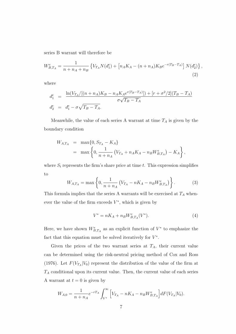
series B warrant will therefore be

W eB,TA

=1

n + nA + nB

{VTA

N(de1) +

[nAKA − (n + nA)KBe−r(TB−TA)

]N(de

2)}

,

(2)

where

de1 =

ln(VTA/[(n + nA)KB − nAKAer(TB−TA)]) + [r + σ2/2](TB − TA)

σ√

TB − TA

de2 = de

1 − σ√

TB − TA.

Meanwhile, the value of each series A warrant at time TA is given by the

boundary condition

WA,TA= max{0, STA

− KA}

= max

{0,

1

n + nA

(VTA

+ nAKA − nBW eB,TA

)− KA

},

where St represents the firm’s share price at time t. This expression simplifies

to

WA,TA= max

{0,

1

n + nA

(VTA

− nKA − nBW eB,TA

)}. (3)

This formula implies that the series A warrants will be exercised at TA when-

ever the value of the firm exceeds V ∗, which is given by

V ∗ = nKA + nBW eB,TA

(V ∗). (4)

Here, we have shown W eB,TA

as an explicit function of V ∗ to emphasize the

fact that this equation must be solved iteratively for V ∗.

Given the prices of the two warrant series at TA, their current value

can be determined using the risk-neutral pricing method of Cox and Ross

(1976). Let F (VTA|V0) represent the distribution of the value of the firm at

TA conditional upon its current value. Then, the current value of each series

A warrant at t = 0 is given by

WA,0 =1

n + nA

e−rTA

∫ ∞

V ∗

[VTA

− nKA − nBW eB,TA

]dF (VTA

|V0).

7

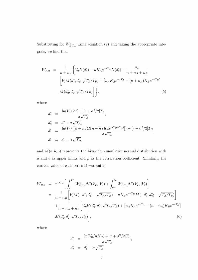
Substituting for W eB,TA

using equation (2) and taking the appropriate inte-

grals, we find that

WA,0 =1

n + nA

{V0N(d∗1) − nKAe−rTAN(d∗2) −

nB

n + nA + nB[V0M(d∗1, d

′1;

√TA/TB) +

[nAKAe−rTA − (n + nA)KBe−rTB

]M(d∗2, d

′2;

√TA/TB)

]}, (5)

where

d∗1 =ln(V0/V

∗) + [r + σ2/2]TA

σ√

TA

,

d∗2 = d∗1 − σ√

TA,

d′1 =ln(V0/[(n + nA)KB − nAKAer(TB−TA)]) + [r + σ2/2]TB

σ√

TB

,

d′2 = d′1 − σ√

TB,

and M(a, b; ρ) represents the bivariate cumulative normal distribution with

a and b as upper limits and ρ as the correlation coefficient. Similarly, the

current value of each series B warrant is

WB,0 = e−rTA

[ ∫ V ∗

0

W uB,TA

dF (VTA|V0) +

∫ ∞

V ∗W e

B,TAdF (VTA

|V0)

]=

1

n + nB

[V0M(−d∗1, d

′′1;−

√TA/TB) − nKBe−rTBM(−d∗2, d

′′2;−

√TA/TB)

]+

1

n + nA + nB

[V0M(d∗1, d

′1;

√TA/TB) +

[nAKAe−rTA − (n + nA)KBe−rTB

]M(d∗2, d

′2;

√TA/TB)

], (6)

where

d′′1 =ln(V0/nKB) + [r + σ2/2]TB

σ√

TB

,

d′′2 = d′′1 − σ√

TB,

8

and the other cumulative normal limits are defined above.

These formulas are perhaps the first sets of theoretical results involving

multiple warrants or contingent firm-based securities in the literature. In

the pricing of the earlier expiry warrant series A in (5), the first two terms

reflect the potential for payoff to exercise of series A warrants when the

underlying per share firm value is sufficiently high compared to KA. The

last and remaining term represents the value of series B warrants in (2) that

must be subtracted from firm value in order to arrive at series A warrant

price. Another way to view a series A warrant is to likened it to a compound

call option, developed by Geske (1979), where if it is exercised at TA, the

stocks are sold and exchanged into series B warrants at market price. There

are two major differences, however, in trying to compare with compound

options or call on call. First, there is a complicated pattern of dilutions

here involving two separate warrants. These dilutions affect the equilibrium

warrant prices in a complicated way. Second, it is simpler in a compound

option when the payment at TA to hold later expiry calls is fixed ex-ante at

KA. However, in our multiple warrant case here, the payment at TA to hold

later expiry warrants is not fixed ex-ante now, but depends on the price of

series B warrants at time TA. This is an important difference which makes

our pricing a level more intricate, and in fact makes the compound option

formulation a special case of our model when there is no dilution, and when

exercise into later series derivatives can be fixed ex-ante. The latter is indeed

a valuable option in itself, and ceteris paribus, would make the compound

option setup more expensive than the multiple warrants setup. This explains

why in (5), the third and last term actually reduce the current equilibrium

price of series A warrants if the underlying firm value is high and there is

high dilution.

For the price of series B warrants in (6), the last term is a simple negative

multiple of the last term in (5). The current price of series A warrants is

9

affected in some inverse manner with the price of later expiry series B war-

rants. As we saw earlier, higher underlying stock price increases moneyness

of series B warrants, enhancing its exercise potential, and thus attenuates

series A warrant price. This subtle attenuation effect that we call the slip-

page effect is not reported in any earlier literature, and is not captured in

compound options literature. Unlike the cross-dilution effect that is more

immediately transparent and that affects the later warrant series, the slip-

page effect affects the earlier warrant series. These effects are interesting and

have implications on an investor who is deciding to invest in both series A

and series B warrants.

Although the risk-neutral pricing method of Cox and Ross (1976) was

used to arrive at the pricing formulas, other derivations are possible. For ex-

ample, the payoff of each warrant series can be duplicated using a dynamic

portfolio of the firm’s equity and riskless bonds. The warrants can then

be competitively priced against this portfolio (see Ross (1978)). Although

the valuation formulas apply only to the case of two series of warrants out-

standing simultaneously, the model can in principle be extended to situations

with three or more series of outstanding warrants using the same backwards

recursive procedure.

The pricing framework developed here can also be used to value other

combinations of derivative securities. For example, slippage and cross-dilution

effects will arise when a firm has two series of convertible bonds outstand-

ing or has one series of convertible bonds and one series of warrants. As

suggested by Geske (1979), this framework is also appropriate for valuing

warrants and other derivatives written on the shares of a firm whose bonds

carry non-trivial default risk. Crouhy and Galai (1994) also investigated the

positive effect of warrant exercise on the firm’s debt value when the debt

carries default risk.

The warrant valuation formulas can be slightly simplified via a change of

10

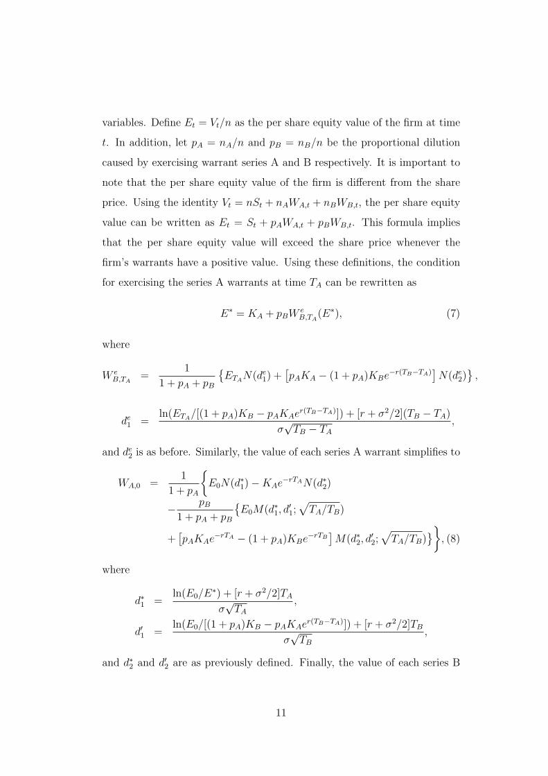
variables. Define Et = Vt/n as the per share equity value of the firm at time

t. In addition, let pA = nA/n and pB = nB/n be the proportional dilution

caused by exercising warrant series A and B respectively. It is important to

note that the per share equity value of the firm is different from the share

price. Using the identity Vt = nSt + nAWA,t + nBWB,t, the per share equity

value can be written as Et = St + pAWA,t + pBWB,t. This formula implies

that the per share equity value will exceed the share price whenever the

firm’s warrants have a positive value. Using these definitions, the condition

for exercising the series A warrants at time TA can be rewritten as

E∗ = KA + pBW eB,TA

(E∗), (7)

where

W eB,TA

=1

1 + pA + pB

{ETA

N(de1) +

[pAKA − (1 + pA)KBe−r(TB−TA)

]N(de

2)}

,

de1 =

ln(ETA/[(1 + pA)KB − pAKAer(TB−TA)]) + [r + σ2/2](TB − TA)

σ√

TB − TA

,

and de2 is as before. Similarly, the value of each series A warrant simplifies to

WA,0 =1

1 + pA

{E0N(d∗1) − KAe−rTAN(d∗2)

− pB

1 + pA + pB

{E0M(d∗1, d

′1;

√TA/TB)

+[pAKAe−rTA − (1 + pA)KBe−rTB

]M(d∗2, d

′2;

√TA/TB)

}}, (8)

where

d∗1 =ln(E0/E

∗) + [r + σ2/2]TA

σ√

TA

,

d′1 =ln(E0/[(1 + pA)KB − pAKAer(TB−TA)]) + [r + σ2/2]TB

σ√

TB

,

and d∗2 and d′2 are as previously defined. Finally, the value of each series B

11

warrant can be rewritten as

WB,0 =1

1 + pB

[E0M(−d∗1, d

′′1;−

√TA/TB) − KBe−rTBM(−d∗2, d

′′2;−

√TA/TB)

]+

1

1 + pA + pB

{E0M(d∗1, d

′1;

√TA/TB) + [pAKAe−rTA − (1 + pA)KBe−rTB ]

M(d∗2, d′2;

√TA/TB)

}, (9)

where

d′′1 =ln(E0/KB) + [r + σ2/2]TB

σ√

TB

and d′′2 is as before. This change of variables eliminates n, the number of out-

standing shares, from the valuation formulas. Focusing on the proportional

dilution of the two warrant series rather than on their absolute dilution allows

additional insights into the model.

Several limiting cases of the model are instructive. When the proportional

dilution of the series A warrants, pA , is zero, valuation formula (9) for the

series B warrants reduces to the Galai-Schellner model. Similarly, valuation

formula (8) for the series A warrants reduces to the Galai-Schellner model

when the proportional dilution of the series B warrants, pB , is zero. When

the proportional dilution of both warrant series is zero, valuation formulas (8)

and (9) both reduce to the Black-Scholes model. Finally, when the maturity

dates and exercise prices of the two warrant series coincide, the two warrant

series merge into one, and the value of each warrant is given by the Galai-

Schellner model with a dilution factor of pA + pB.

3 Comparison to Other Models

To determine the potential benefits of using the multiple warrants model,

theoretical prices under this model are compared against those predicted by

existing models. The Black-Scholes (1973) and Galai-Schneller (1978) mod-

els are used for this comparison because they are better-known and more

12

frequently cited by leading derivatives texts such as Hull (2000). For a given

set of parameters, the theoretically correct prices of the two warrant series

are calculated using our multiple warrants model. Then, based on the same

parameters, the prices predicted by the Black-Scholes and Galai-Schneller

models are computed. The percentage pricing errors of the two models rel-

ative to our model are used as measures of their performance.5 This perfor-

mance measure is intended to provide an indication of the extent of pricing

errors when using popular models on multiple warrants.

For each scenario, the per share value of the firm was arbitrarily set

to $10. The pricing errors of the Black-Scholes and Galai-Schneller models

were found relatively insensitive to changes in the riskless interest rate and

return variance for the firm, so these were each fixed at 5% for the scenarios

presented here. It should be noted that the appropriate return variances for

the Black-Scholes and Galai-Schneller models are different from the return

variance for the firm. The input for the Black-Scholes model is the return

variance on the firm’s shares while the Galai-Schneller model uses the return

variance on a portfolio of the firm’s shares and the warrant being valued.

The conditional variances that were consistent with a 5% return variance

for the firm and the relative prices of the firm’s shares and warrants were

used for these models.6 The proportional dilution of the warrants were set at

5Alternatively, the absolute pricing error could be been used to indicate the goodness-

of-fit of the two models. However, because most investors care more about percentage

returns than absolute dollar gains, percentage pricing error is more relevant to them.6The identity Vt = nSt + nAWA,t + nBWB,t shown earlier was used to derive the

volatility of per share return for the Black-Scholes model, and volatility of per share equity

return, incorporating only the relevant warrant series, for the Galai-Schneller model. These

volatility inputs are computed conditional, or given, the volatility of dVt/Vt set to 5%. As

pointed out by a referee, the state variable underlying the three different models are not

identical. Keeping firm value volatility constant is generally not consistent with constant

volatilities for the other models. Therefore, the ensuing comparison in Table 1 is subject

to this limitation.

13

2.5% for both series (low dilution) and at 10% (high dilution). Three series

of expiry terms were considered: 12

year for series A and 1 year for series B

(both series near expiry), 12

year for series A and 4 years for series B (one

series near expiry), and 3 years for series A and 4 years for series B (neither

series near expiry). Finally, exercise prices of $9, $12, and $20 were used for

the series A warrants, while prices of $10, $14, and $25 were used for the

series B warrants. In all, prices were generated for 24 different scenarios.

The results of this valuation exercise are presented in Table 1. Both

models on average overprice the series A and series B warrants. The Galai-

Schneller model performs generally better at pricing the two warrant series

than does the Black-Scholes model. The average pricing error across the

24 scenarios is 0.82% for the Galai-Schneller model and 2.5% for the Black-

Scholes model. This result shows that the Galai-Schneller model outperforms

the Black-Scholes model when it comes to valuing warrants. Handley (2002)

pointed out that in an informationally efficient market, expected dilution

would be implicitly taken into account by being conditionally reflected in

the underlying stock price. Thus, the difference in performance cannot be

solely attributed to the explicit provision of dilution in the Galai-Schneller

model.

The pricing error for both models increases as the proportional dilution

of the two warrants rises. When the potential dilution of the two warrant

series is only 2.5%, the average mispricing across the 12 scenarios is 0.36%

for the Galai-Schneller model and 0.98% for the Black-Scholes model. This

mispricing increases to 1.28% and 4.06% when the potential dilution rises

to 10%. Thus, dilution factor also affects the Galai-Schneller model in the

multiple warrant case.

The pricing error of the two models also appears to increase as the time

to expiration increases. The average pricing errors across both dilution cate-

gories are also larger for series B warrants relative to series A warrants. The

14

Black-scholes model misprices the series A warrants by an average of 1.95%

as compared to 3.09% for the series B warrants. Similarly, the average pric-

ing error of the Galai-Schneller model is 0.59% for the series A warrants and

1.05% for the series B warrants.

Finally, the pricing error for the two models tends to increase as the

exercise price rises, or when the moneyness of the warrants decreases. For

series A warrant with 12

year to expiry, the maximum reported mispricing

by the Galai-Schneller model is only -0.3% when the exercise price of these

warrants is $9. This increases to 2.8% when the exercise price is $12. A

similar pattern is observed for mispricing under the Black-Scholes model.

The same phenomenon is observed for series B warrants as well.

This analysis shows that the highest pricing errors for the Black-Scholes

and Galai-Schneller models occur when the potential dilution of the warrants

is high, when the warrants are out-of-the-money, or when the warrants are

further from expiry. Therefore, these are the conditions under which the

multiple warrants pricing model will be most beneficial to investors, and

where the simpler single warrant models will not be accurate.

The comparative results provide an interesting observation that shows

the important relations between multiple warrants. We observe that the

Galai-Schneller model overprices both the series A warrants and the series

B warrants relative to our multiple warrant model. Intuitively, what hap-

pens is that for series A warrant, the slippage caused by the presence of

the longer expiry series B warrants tends to diminish series A’s price. The

Galai-Schneller or Black-Scholes model does not consider this effect, because

they are based on a single warrant formulation, and so overprices. For series

B warrants, the cross-dilution effect from series A also tends to diminish its

price. Thus the Galai-Schneller or Black-Scholes model again overprice.

Below we consider a practical example to illustrate how the model can

be used to price the multiple warrants. In the process, we also illustrate the

15

presence of the slippage and the cross dilution effects. Prices are computed

as at August 21, 2002. Two warrants are simultaneously issued by the Strike

Engineering Company in Singapore, viz. Singapore Exchange security codes

W 031220 and W 060405.

W 031220 has an outstanding issue of 146,603,000 warrants. The con-

version ratio is 1 warrant to 1 share. The exercise price is S$0.07 per share.

Expiry date of warrant is December 20, 2003. The closing price of the warrant

at August 21, 2002 is S$0.015. Time to expiration is TA = 1.329 years.

W 060405 has an outstanding issue of 193,239,985 warrants. The con-

version ratio is 1 warrant to 1 share. The exercise price is S$0.11 per share.

Expiry Date of warrant is April 5, 2006. The closing price of the warrant at

August 21, 2002 is S$0.02. Time to expiration is TB = 3.589 years.

The underlying Strike Engineering ordinary shares have an issued volume

of 879,618,000 shares. The riskfree interest rate is 2% per annum. The un-

derlying stock closing price at August 21, 2002 is S$0.04. For this illustration,

we employ the volume-weighted average of implied volatility of Black-Scholes

warrant price of W 031220 and of W 060405. This volatility is used for all

the models.

The series A W 031220 warrants price, WA,0, and the series B W 060405

warrants price, WB,0 are computed based on the model developed into section

2. The model price for W 031220 is $0.012 per warrant compared with $0.013

calculated using the Galai-Schneller model. We can clearly see the slippage

effect that makes the model price lower than the GS price for the shorter life

warrants. The model price for W 060405 is $0.020 per warrant compared

with $0.022 calculated using the Galai-Schneller model. Here, we can clearly

see the cross dilution effect that makes the model price lower than the GS

price for the longer life warrants.

16

4 Hedging Ratios

The value of each warrant is an explicit function of 10 variables: E0, KA,

KB, TA, TB, pA, pB, σ, r, and E∗. However, E∗ is itself an implicit function

of all the other variables except E0. Therefore, the complete functional form

of the series A warrants is

WA,0(E0, KA, TA, pA, σ, r, KB, TB, pB, E∗(KA, TA, pA, σ, r, KB, TB, pB)).

This implies that, for example, the delta of the series A warrant is

δ(WA,0) =∂WA,0

∂E0

∣∣∣∣∣E∗

+∂WA,0

∂E∗∂E∗

∂E0

.

The last term in this equation, as in other Greeks, ∂E∗/∂(·) must be deter-

mined by partially differentiating equation (7) with respect to the parameter

(·) and then solving the equation.

More specifically, applying calculus,

δ(WA,0) =1

1 + pA

{N(d∗1) +

1

σ√

2πTA

exp(−(d∗1)2/2) − KAe−rTA

σE0

√2πTA

exp(−(d∗2)2/2)

}

− pB

(1 + pA + pB)(1 + pA)

{1

σ√

2πTA

exp(−(d∗1)2/2)N

(d′1 −√

TA/TBd∗1√1 − TA/TB

)+

exp(−(d′1)2/2)

σ√

2πTB

N(d∗1 −

√TA/TBd′1√

1 − TA/TB

)+ M(d∗1, d

′1;

√TA/TB)

}

−pB[pAKAe−rTA − (1 + pA)KBe−rTB ]

(1 + pA + pB)(1 + pA){exp(−(d∗2)

2/2)

σE0

√2πTA

N(d′2 −

√TA/TBd∗2√

1 − TA/TB

)+

exp(−(d′2)2/2)

σE0

√2πTB

N(d∗2 −

√TA/TBd′2√

1 − TA/TB

)}.

Similarly, the delta of the series B warrant is

δ(WB,0) =∂WB,0

∂E0

∣∣∣∣∣E∗

+∂WB,0

∂E∗∂E∗

∂E0

.

17

δ(WB,0) =1

1 + pB

{−exp(−(d∗1)

2/2)

σ√

2πTA

N(d′′1 −

√TA/TBd∗1√

1 − TA/TB

)+ M(−d∗1, d

′′1;−

√TA/TB)

+exp(−(d′′1)

2/2)

σ√

2πTB

N(−

d∗1 −√

TA/TBd′′1√1 − TA/TB

)+

KB exp(−rTB − (d∗2)2/2)

σE0

√2πTA

N(d′′2 −

√TA/TBd∗2√

1 − TA/TB

)−KB exp(−rTB − (d′′2)

2/2)

σE0

√2πTB

N(d∗2 −

√TA/TBd′′2√

1 − TA/TB

)+

1

(1 + pA + pB)

{exp(−(d∗1)

2/2)

σ√

2πTA

N(d′1 −

√TA/TBd∗1√

1 − TA/TB

)+

exp(−(d′1)2/2)

σ√

2πTB

N(d∗1 −

√TA/TBd′1√

1 − TA/TB

)+ M(d∗1, d

′1;

√TA/TB)

}

+pAKAe−rTA − (1 + pA)KBe−rTB

(1 + pA + pB){exp(−(d∗2)

2/2)

σE0

√2πTA

N(d′2 −

√TA/TBd∗2√

1 − TA/TB

)+

exp(−(d′2)2/2)

σE0

√2πTB

N(d∗2 −

√TA/TBd′2√

1 − TA/TB

)}.

The delta δ(WA,0) is positive as expected. The delta value is typically

smaller than that in Black-Scholes not just due to dilution. Intuitively, this is

because as E0 increases, WB,0 will also increase and will cause some slippage

in the price of WA,0 as discussed in the previous section. It is also interesting

to note that in the case of multiple warrants, the expiry time TB also affects

delta here. If TB increases and is more distant from TA, then the δ(WA,0)

increases.

Likewise, the Greeks7 of the series B warrants can be similarly found. As

expected, δ(WB,0) > 0.

7The other Greeks such as gamma, theta, rho, and vega, are also derived. However,

they are too lengthy to be reported here. Interested readers may write to the authors for

a copy of these results.

18

5 Conclusions

Warrants are an important class of funding securities in almost all security

markets worldwide. Warrants became very popular in the fast emerging stock

markets of Asia in the late 1980s and early 1990s. In some countries such

as Switzerland, Malaysia, and Singapore, the issue of multiple series of stock

purchase warrants by the same firm is common. stock purchase warrants

result in new shares being issued when they are exercised. The issue of new

shares leads to price dilution, which makes warrant pricing different in some

ways from exchange or OTC call option pricing. This phenomenon has been

addressed in the literature, notably by Black and Scholes (1973), and Galai

and Schneller (1978).

However, the dilution pattern in the case of multiple warrants is intri-

cate. We show that there is a subtle slippage effect that causes the earlier

series warrants to be overpriced using Galai-Schneller model, and a cross di-

lution effect that causes the later series warrants also to be overpriced by the

same Galai-Schneller model. The latter model already accounts for the usual

dilution in a single warrant pricing model.

Our analysis shows that the highest pricing errors for the Black-Scholes

and Galai-Schneller models occur when the potential dilution of the warrants

is high, when the warrants are out-of-the-money, or when the warrants are

further from expiry. The average mispricing for the earlier expiry series A

warrants is shown to be lower than for the later expiry series B warrants.

Intuitively, the cross-dilution effect is stronger than the more subtle slippage

effect.

This paper provides the appropriate pricing formula to use when multiple

stock purchase warrants are encountered. It should add a useful contribution

to the literature on warrant pricing. Potential avenues for further research

include the empirical test of multiple warrants model, strategic exercise of

19

multiple warrants, and the impact of extending the expiry if the warrants

become too far out-of-the-money. The latter issue is common in situations

where warrants are an important class of security for funding purpose in the

capital market.

20

References

Black, Fisher, and Myron Scholes, 1973, ”The pricing of options and corpo-

rate liabilities,” Journal of Political Economy, 81, 637-659.

Constantinides, George, 1984, ”Warrant Exercise and Bond Conversion in

Competitive Markets,” Journal of Financial Economics, 13, 371-397.

Cox, John C., and Stephen A. Ross, 1976, ”The valuation of options for

alternative stochastic processes,” Journal of Financial Economics, 3, 145-

166.

Crouhy, M., and D. Galai, 1994, ”The interaction between the financial and

investment decisions of the firm: The case of issuing warrants in a levered

firm,” Journal of Banking and Finance, 18, 861-880.

Emanuel, David, 1983, ”Warrant valuation and exercise strategy,” Journal

of Financial Economics, 12, 211-236.

Galai, Dan, and Mier I. Schneller, 1978, ”Pricing of warrants and the value

of the firm,” Journal of Finance, 33, 1333-1342.

Geske, Robert, 1979, ”The valuation of compound options,” Journal of Fi-

nancial Economics, 7, 63-81.

Handley, J.C., 2002, ”On the valuation of warrants,” Journal of Futures

Markets, forthcoming.

Hull, John C., 2000, Options, Futures, and Other Derivatives, 4th Edition,

NJ: Prentice-Hall.

Lauterbach, Beni, and Paul Schultz, 1990, ”Pricing warrants: An empirical

study of the Black-Scholes model and its alternatives,” Journal of Finance,

45, 1181-1209.

21

Merton, Robert C., 1976, ”Option pricing when underlying stock returns are

discontinuous”, Journal of Financial Economics, 3, 125-144.

Roll, Richard, 1977, ”An analytical valuation formula for unprotected Amer-

ican call options on stocks with known dividends”, Journal of Financial Eco-

nomics 5, 251-258.

Ross, Stephen, 1978, ”A simple approach to the valuation of risky streams,”

Journal of Business, 51, 453-475.

Spatt, Chester S., and Frederic P. Sterbenz, 1988, ”Warrant Exercise, Div-

idends, and Reinvestment Policy,” Journal of Finance, 43, No. 2, 493-506.

22

Table 1: Mispricing of Galai-Schneller and Black-Scholes modelsfor multiple warrantsa

Series A Warrants Series B WarrantsFair G-S model B-S model Fair G-S model B-S model

KA KB T bA T b

B value error error value error error

Low dilution: pA = pB = 2.5%$9 $10 1

21 $1.333 -0.1% -0.1% $1.072 0.1% 0.0%

9 14 12

1 1.356 0.0 -0.1 0.107 0.4 1.69 14 1

24 1.332 0.0 -0.1 1.180 0.0 0.2

9 25 12

4 1.355 0.0 -0.1 0.130 -1.2 0.312 10 1

21 0.129 0.7 1.6 1.103 -0.1 -0.2

12 14 12

1 0.138 0.4 1.2 0.115 1.6 2.812 14 1

24 0.131 0.2 1.1 1.215 0.0 0.1

12 25 12

4 0.139 0.1 1.0 0.138 0.8 2.312 14 3 4 1.340 0.0 0.0 1.188 0.2 0.412 25 3 4 1.364 -0.1 0.0 0.131 1.6 3.120 14 3 4 0.167 1.4 2.8 1.219 -0.1 0.020 25 3 4 0.176 0.7 2.0 0.137 2.0 3.6

High dilution: pA = pB = 10%9 10 1

21 1.185 -0.3 -0.5 0.916 0.3 0.2

9 14 12

1 1.259 -0.1 -0.3 0.075 1.2 6.99 14 1

24 1.184 -0.2 -0.4 0.995 0.1 0.9

9 25 12

4 1.258 0.0 -0.3 0.094 -5.5 0.712 10 1

21 0.096 2.8 7.2 1.021 -0.5 -0.6

12 14 12

1 0.124 1.0 4.7 0.097 6.3 11.812 14 1

24 0.103 -0.2 3.9 1.115 0.1 0.7

12 25 12

4 0.127 -0.1 3.5 0.119 2.9 9.212 14 3 4 1.186 -0.1 0.1 1.025 1.0 1.712 25 3 4 1.266 -0.2 0.0 0.096 6.5 13.520 14 3 4 0.128 5.9 11.9 1.128 -0.4 0.120 25 3 4 0.158 2.3 7.7 0.117 8.0 14.8

a Calculations are based on a per share equity value of $10.00, a risklessinterest rate of 5%, and a return variance of 5% for the firm. The variancesused in the Galai-Schneller and Black-Scholes models are those that are con-sistent with a 5% return variance for the firm and the relative values of thefirm’s shares and warrants.b Time to expiration is stated in years.

23