The Use of Tensegrity to Simulate Diaphragm Motion Through ...

Imperial College LondonDepartment of Computing

The Use of Tensegrity to SimulateDiaphragm Motion ThroughMuscle and Rib Kinematics

Author:Wesley Bourne

Supervisors:Dr. Fernando Bello

Dr Pierre-Frederic Villard

Third Year BEng Project

Project Directory: http://www.doc.ic.ac.uk/˜wlb05/project/

Abstract

Respiration is a complex process involving the interaction of several musclesand other tissue. The diaphragm has a large influence as it is the centraldivision within the abdomen and plays a role in inflating and deflating thelungs. It is composed of di!erent kinds of tissue which need to be modelledusing di!erent paradigms. Tensegrity is the use of rigid and elastic linksto give more rigidity to systems and will be used to model the more rigidparts of the diaphragm. A mass spring will be used for the remainder.Rib kinematics and attached tissues will also be modelled to provide a morerealistic simulation. The result is a Java simulation running in real time withparameters to control breathing speed, force, rib motion and mass springparameters. The results can be exported and an evaluation of the simulatorwill be provided.

1

Acknowledgements

• My thanks go to Fernando Bello and Pierre-Frederic Villard for theirconsistent, fast and constructive advice throughout the project.

• I would also like to thank Philip Edwards for agreeing to be my secondmarker.

• Finally, I would like to thank my parents for giving me the opportunityto study at Imperial College.

2

Contents

1 Introduction 51.1 Motivation and Intent . . . . . . . . . . . . . . . . . . . . . . 51.2 Goals . . . . . . . . . . . . . . . . . . . . . . . . . . . . . . . 51.3 Salient Points . . . . . . . . . . . . . . . . . . . . . . . . . . . 51.4 Contributions . . . . . . . . . . . . . . . . . . . . . . . . . . . 6

2 Background 72.1 Medical Simulation . . . . . . . . . . . . . . . . . . . . . . . . 7

2.1.1 Requirements . . . . . . . . . . . . . . . . . . . . . . . 72.1.2 3D Imaging Techniques . . . . . . . . . . . . . . . . . 82.1.3 Sample Current Applications . . . . . . . . . . . . . . 10

2.2 Mass Spring Systems . . . . . . . . . . . . . . . . . . . . . . . 102.2.1 Equation of Dynamics . . . . . . . . . . . . . . . . . . 112.2.2 Explicit Euler Solver . . . . . . . . . . . . . . . . . . . 122.2.3 Choice of !t . . . . . . . . . . . . . . . . . . . . . . . . 13

2.3 Finite Element Method . . . . . . . . . . . . . . . . . . . . . 142.4 Tensegrity . . . . . . . . . . . . . . . . . . . . . . . . . . . . . 16

2.4.1 Definition and Origins . . . . . . . . . . . . . . . . . . 162.4.2 Method . . . . . . . . . . . . . . . . . . . . . . . . . . 172.4.3 Applying Tensegrity Constraints . . . . . . . . . . . . 172.4.4 Potential Application to Tissue Simulation . . . . . . 18

2.5 Diaphragm Modelling . . . . . . . . . . . . . . . . . . . . . . 192.5.1 Anatomy and Physiology . . . . . . . . . . . . . . . . 202.5.2 Diaphragm Composition . . . . . . . . . . . . . . . . . 21

3 Biomechanical Modelling 223.1 Diaphragm Mechanics and Tensegrity . . . . . . . . . . . . . 223.2 Rigid Connections . . . . . . . . . . . . . . . . . . . . . . . . 243.3 Fixed Points . . . . . . . . . . . . . . . . . . . . . . . . . . . 263.4 Action Lines . . . . . . . . . . . . . . . . . . . . . . . . . . . 283.5 Rib Kinematics . . . . . . . . . . . . . . . . . . . . . . . . . . 29

3

4 Implementation 304.1 SOFA Solution . . . . . . . . . . . . . . . . . . . . . . . . . . 30

4.1.1 Background . . . . . . . . . . . . . . . . . . . . . . . . 304.1.2 Diaphragm Motion in SOFA . . . . . . . . . . . . . . 314.1.3 Issues with Heterogenity . . . . . . . . . . . . . . . . . 33

4.2 Java Solution . . . . . . . . . . . . . . . . . . . . . . . . . . . 344.2.1 Basic Class Structure . . . . . . . . . . . . . . . . . . 344.2.2 2D Display . . . . . . . . . . . . . . . . . . . . . . . . 354.2.3 3D Display . . . . . . . . . . . . . . . . . . . . . . . . 36

4.3 The Final Product . . . . . . . . . . . . . . . . . . . . . . . . 38

5 Evaluation 415.1 Tensegrity . . . . . . . . . . . . . . . . . . . . . . . . . . . . . 41

5.1.1 E!ect on Diaphragm . . . . . . . . . . . . . . . . . . . 435.2 Diaphragm Motion . . . . . . . . . . . . . . . . . . . . . . . . 45

5.2.1 The Patient Model . . . . . . . . . . . . . . . . . . . . 465.3 Simulator . . . . . . . . . . . . . . . . . . . . . . . . . . . . . 46

5.3.1 Cube Simulation . . . . . . . . . . . . . . . . . . . . . 475.3.2 Diaphragm Simulation . . . . . . . . . . . . . . . . . . 485.3.3 Influence of Mesh Size with a Heterogeneous Model . 495.3.4 Influence of Mesh Size with a Homogenous Model . . 505.3.5 Conclusions . . . . . . . . . . . . . . . . . . . . . . . . 52

6 Conclusion 556.1 Discussion . . . . . . . . . . . . . . . . . . . . . . . . . . . . . 55

6.1.1 Work Completed . . . . . . . . . . . . . . . . . . . . . 556.1.2 Project Outcomes . . . . . . . . . . . . . . . . . . . . 556.1.3 Limitations . . . . . . . . . . . . . . . . . . . . . . . . 55

6.2 Future work . . . . . . . . . . . . . . . . . . . . . . . . . . . . 566.2.1 Integration with SOFA . . . . . . . . . . . . . . . . . . 566.2.2 Educational Context . . . . . . . . . . . . . . . . . . . 566.2.3 Haptic Integration . . . . . . . . . . . . . . . . . . . . 56

Bibliography 57

A Appendix 59A.1 User Guidance . . . . . . . . . . . . . . . . . . . . . . . . . . 59

A.1.1 Adding a new object . . . . . . . . . . . . . . . . . . . 59A.1.2 Action Line Fall O! Modication . . . . . . . . . . . . 62A.1.3 Euler Solver Implementation . . . . . . . . . . . . . . 62

4

Chapter 1

Introduction

1.1 Motivation and Intent

The diaphragm plays a key role in the respiration of humans and its complexmotion can have an impact on interventional or therapeutic procedures. It ismostly muscular and divides the torso, connected to the spine and ribs, withholes through which large blood vessels pass into the lower abdomen. Theposition of the diaphragm and its deformation are influenced by rib motioncombined with muscle action. This project aims to model the motion anddeformation of the diaphragm together with the surrounding organs andbones, using a combination of mass spring systems and tensegrity. Chapter 2describes these methods together with the powerful and widely used finiteelement method. Due to the complicated interactions between neighbouringtissues, assumptions had to be made and heuristic algorithms applied. Seechapter 3 for a more in depth discussion of this aspect of the project.

1.2 Goals

The goal of the project is to create a simulation of diaphragm motion usingtensegrity to model the more rigid upper regions. The simulation needs tobe real-time and tuneable via a control panel to allow it to easily match thebreathing motion obtained from patient scans.

1.3 Salient Points

In order to understand the validation section of the report, it is importantto have a basic understanding of the process whereby CT scans are filtered,segmented and meshed. This is illustrated at the beginning of chapter 2. An-other important aspect of the project is the inability of the SOFA frameworkto process two tissue simulation methods on the same model. This resulted

5

in having to implement the simulation outside the SOFA framework as orig-inally planned, using Java and OpenGL instead. The full discussion of thisproblem is presented in section 4.1.3.

Finally, the simulator(figure 1.1) was complete and an evaluation on thee!ect of tensegrity is shown in chapter 5.

Figure 1.1: The completed Java simulator with the ribs, diaphragm, lungssternum and ligaments visible.

1.4 Contributions

• Tuneable Simulator : The final product is a simulator with parametersto change the speed, magnitude of forces and other factors contribut-ing to the diaphragm motion. This allows the simulator to matchdiaphragmatic or chest breathing and any mix in between.

• Customisable to Patients: The simulator has been tested on threepatients and performs realistically thanks to the tuneable parameters.

• Extensible Framework : The project is extendable and object-orientatedand is amenable to future work by other researchers or intern students.

• Study and Analysis of Computational Cost of Tensegrity: The cost ofsolving simulations involving rigid links has been studied and evalu-ated.

• Study into Applicability of Tensegrity: Tensegrity has been shown tohave a supportive e!ect as a part of a tissue simulator.

• Algorithms for Diaphragm Initiation and Muscle Motion: Intuitivealgorithms have been created that link opposing sides of tissue topolo-gies and simulate the attachment of tissue to other models and applymuscle forces.

6

Chapter 2

Background

The aim of this background section is to make this document self-containedand also to give a general understanding of the field. The discussions herecan be expanded more fully in the work of Meier et al[ML] and Vidal etal[VB]. The section will begin with a brief summary of the current field ofmedical simulation before moving to simulating tissue and ending with thephysiology of the diaphragm. The description of the kinematic equations isbased on the work of Bara! and Witkin[BW] and uses the syntax of Bhasinand Liu[BL],

2.1 Medical Simulation

Medicine has always been a great follower of technology and the growth inpossibilities and computational power have been closely followed by thosewanting to use these advances for medical purposes. Being such a massivefield, there are numerous applications including medical diagnosis, training,planning and more. Another contributing factor to the rapid growth ofsimulation is the wider availability of data from CT, MRI and other 3Dforms of medical information. Computers are excellent at summarising,manipulating and finding patterns in large datasets. Their input to medicalprocedures can prove invaluable.

2.1.1 Requirements

In such a high-pressure and demanding environment, any simulation mustreach a level of realism and usability. The simulation must be:

• Validated : Experts in the field must verify the validity of the simula-tion as a useful tool.

• Realistic: There is no need for a simulation that varies so much fromthe truth that it may give an inconsistent or false impression of realityand put the patient in danger.

7

• A!ordable: Hospital budgets must take into account which invest-ments will give the greatest benefit to the overall population. A veryexpensive simulation will deter investment.

2.1.2 3D Imaging Techniques

Filtering

Figure 2.1: The start and end points of filtering of a diaphragm.

Information entered into a computer via a scanner will most likely containnoise. Filtering is the process by which this noise is removed by smoothingor blurring each pixel based on a combination of its neighbours. This isvisible in figure 2.1. In medical simulations, this can remove crucial detailabout anatomical boundaries. A more involved technique using anisotropicdi!usion aims to iterate towards an equilibrium state controlled by a partialdi!erential equation. It has proved successful and is a popular choice toimprove image quality.

Segmentation

Figure 2.2: The start and end points of segmentation of a diaphragm. Asequence of slices from a 3D scan is turned into labelled voxels.

Once an image has been filtered to remove any noise, it is desirable to beable to label the di!erent anatomical areas of the image(figure 2.2). This is

8

a time-consuming process and is reliant on the user. Techniques include:

• Thresholding : A value is chosen to be a threshold and the image ispartitioned based on those that fall on either side of this boundary.

• Region Growing : A centre point is chosen as a seed and this region isgrown up to a boundary.

• Watershed transform: An intuitively simple algorithm which dividesthe image based on basins and hills as if water were flooded into thescene.

• Livewire: A user’s cursor is tracked and the closest approximatedboundary is selected before being approved by the user who can thenproceed to the next point.

Meshing

Figure 2.3: The meshing process begins with mutiple slices of segmenteddata and proceeds to a 3D model.

After the slices of a scan have been segmented into the di!erent organs, ameshing algorithm can be used to create a mesh(figure 2.3). Here are somepopular methods:

• Delaunay : In 2D, for a set of points P, the Delaunay triangulationmaximises the minimum angle in the triangles created, thus preventingthe creation of sliver triangles. The method is more complicated butintuitively similar in 3D.

• Marching Cubes: Is the 3D equivalent of the marching squares al-gorithm. The algorithm traverses the scalar field considering eightneighbouring positions at a time. It determines the polygons needed torepresent this part of the isosurface passing through this cube. Thesepolygons are then fused to create the surface.

9

2.1.3 Sample Current Applications

As a result of the funding and interest applied to medicine there are aplethora of interesting and advanced applications. A brief description ofexamples are shown here.

Augmented Reality

Computer-generated artefacts are added to a scene in the real world. Theuser typically has a head-mounted display. The display can aid in the dif-ferentiation of tissue or help guide an instrument. The additions made viathe computer must be correctly orientated with the position of the user.Performing this synchronisation can prove to be very di"cult; without nearperfect alignment the slightest discrepancies can become a hindrance.

Virtual Endoscopy

In a traditional video endoscopy, an endoscope is inserted into the patientwith a small opening in the body. This is an invasive procedure and onlyhas limited viewing ability. A virtual endoscopy creates a simulation inwhich a virtual endoscope can be manoeuvred through the patient in a 3Denvironment created using a medical scan of the patient. It allows for theinteractive exploration of the tissues and removes the need for an invasiveprocedure.

Patient Specific Virtual Environments

Using prior data from the patient a simulation can be tailored to an exactspecification. This means the surgeon can practise a procedure in an envi-ronment as near to reality as possible. This possibility allows the surgeonto be more confident and prepare for any technically challenging elementsduring the operation.

2.2 Mass Spring Systems

Once it has been decided that a medical simulation is needed, there is arequirement for accurate and real-time modelling of tissue. Popular methodsto simulate tissue are presented in the following section. Mass spring, Finiteelement and Tensegrity methods will be discussed.

Mass spring systems are a popular and e!ective way of simulating avariety of physical interactions. A set of masses is created with predefinedlinks. A subsection of a simple mass spring system is shown in figure 2.4.These links have sti!ness values and they exert forces on the masses whichin turn move. Iteratively solving and analysing the motion of the masses canbe used to simulate objects as varied as cloth or human organs. A standard

10

method of defining the forces and solving the motion is discussed in thefollowing section.

Figure 2.4: A 2D mass spring system, mass i has three neighbours whichmust be included in its force calculation.

Advantages DistadvantagesQuick Visualisation: Simplicity be-tween the mesh and the simulationmeans it is quick to implement.Simulation Speed : Equations of mo-tion are fast and e"cient to solve.Mature Method : There has beena substantial amount of researchbacking the method and althoughit isn’t perfect, it performs well inmany situations.

Reliance on Mesh: A mesh thatlooks identical to another may per-form very di!erently as a result ofdi!erent low-level connections andconstructs.Speed of Propagation: Forces canonly propagate one neighbour at atime. This removes from the real-ism.Tendency to Oscillate: The simu-lation can get into a state wheremasses oscillate. This is discussedfurther in section 2.2.3.

2.2.1 Equation of Dynamics

Equation 2.1 forms the basis of the forces that are calculated within thesystem. It is computed for each mass at the beginning of each timestepbefore being used along with the current position and velocity to numerically

11

integrate to find the position at the next timestep.The equation indicates that the resultant force felt by a mass is the sum

of all the forces of tensile links and any outside force minus any frictionforce.

f ti = mia

ti =

!

"#

j!N(i)

kij dij$ltij ! l0ij

%&

' + f te ! "vt

i (2.1)

Where:f t

i is the force placed on mi at time t.mi is a mass i.at

i is the acceleration of a mass i at time t.N(i) is the set of neighbouring masses.dij is the distance between mi and mj .ltij is the distance between mi and mj at time t.l0ij is the distance between mi and mj at rest.f t

e is an external force on the mass at time t, such as gravity." is the friction coe"cient.vti is the velocity of mi at time t.

Manipulating equation 2.1 yields the following:

ati =

(()j!N(i) kij dij

(ltij ! l0ij

**! "vt

i + f te

*

mi(2.2)

The Continuous Solution

f = ma (2.3)

vti =

+ t

0f(ai) da. (2.4)

xti =

+ t

0f(vi) dv. (2.5)

These continuous equations become discretised and are solved using the Eu-ler method. They describe standard Newtonian physics where acceleration,velocity and position are interrelated via integrals and derivatives. The sim-ulation uses a discrete timestep of milliseconds and for this reason theseequations must be approximated.

2.2.2 Explicit Euler Solver

The Discrete Approximation

Once all the forces have been calculated using the force equation presentedin equation 2.1, the analytic equations 2.4 and 2.5 must be discretised. The

12

chosen solution for the implementation was an explicit Euler solver. TheEuler method uses the following intuitive approximations.

vt+!ti = vt

i + ati!t (2.6)

xt+!ti = xt

i + vt+!ti !t (2.7)

These equations are easy to solve and lend themselves well to scaling mean-ing that real-time simulation is possible.

Figure 2.5: The Euler Integration method shown graphically.

2.2.3 Choice of !t

After considering figure 2.5, it becomes apparent that the correct choice of!t makes a massive di!erence in the convergence of any solution. Some ofthe possible convergent cases are shown in figure 2.6. Choosing too smalla value leads to a case where there may be little movement and frictionmay counteract any motion towards a true solution. Choosing a value toolarge may lead to the simulation ‘exploding’. Both are very undesirable andthis issue leads to a great deal of time in mass spring systems being spenton tuning parameters to arrive at a satisfactory tradeo! between speed ofsolution and stability.

13

Figure 2.6: Di!erent convergent and divergent cases.

2.3 Finite Element Method

Rather than basing the deformation model on a discontinuous approach,an alternative has been proposed which is based on the law of continuummechanics computed in a continuous medium. Once assumptions have beenmade about the elasticity and the lack of internal forces, the following secondorder Navier equation arises[ML].

(# + µ) grad(div u) + µ!u = 0 (2.8)

Where:# and µ are the Lame constants of the material.u is the displacement vector of any point of the object with respect

to its initial position.grad is the gradient function: grad(x, y, z) =

("f"x , "f

"y , "f"z

*

div is the divergence function: div(x, y, z) = "f"x + "f

"y + "f"z

An analytic solution to this equation does not exist and therefore a nu-merical solution is required. The FEM method aims to solve this equationby subdividing the object into a discrete number of elements. Once this hasbeen completed, the displacement of each one of these elements is approxi-mated by a polynomial equation which is related to control nodes.

A system of equations arises:

KU = F (2.9)

14

Where:K is the symmetric and spare sti!ness matrix.U is the nodal displacement vector.F is the force vector.

Solving this equation yields the displacement of each node at that iter-ation.

Advantages DistadvantagesBased on Physics: Unlike massspring systems, the quality of thesimulation doesn’t depend on themesh.

Speed : The method is much morecomputationally expensive. Realtime simulation is only possible for arelatively small number of elements.Hard to program: The method ismore involved than the mass springsystem and is much harder to im-plement. Most people use a com-mercial FEM package, but these areusually not real time.

2.4 Tensegrity

2.4.1 Definition and Origins

Figure 2.7: A simple figure demonstrating tensegrity. The solid bars repre-sent rigid links.

Tensegrity is a portmanteau of tensional integrity. This arises from its use ofboth rigid and elastic links in order to form a stable structure(figure 2.7). In

15

1927 architect R. Buckminster Fuller investigated its uses in buildings[IN].Later, artist Kenneth Snelson created structures involving tensegrity. Hisstructure is shown in figure 2.8.

Figure 2.8: One of Snelson’s tensegretic structures.

2.4.2 Method

The presence of elastic links adds a direct correspondence with the workingsof mass spring systems. For this reason, mass spring systems (section 2.2)are usually the starting point in developing tensegrity. Constraining thesimulation to follow the properties of the rigid links is the main challenge.

2.4.3 Applying Tensegrity Constraints

Figure 2.9: A diagram to help explain the solution to enforcing the tensegrityconstraint. Apre,Bpre signify the position before motion. Amid,Bmid are thelocations ignoring the length constraint. Apost,Bpost are the final locationsafter applying the constraint.

16

Once tensile and rigid connections have been created, an algorithm is re-quired to ensure the length of the rigid connections are respected throughoutthe kinematic motion. A solution was found in the work of Alexis Guillaume[GU]. It proceeds by calculating the location of each mass ignoring all rigidconnections and updating their locations. Post-processing is then used tomodify the locations of the masses that have rigid connections.

ApreAmid

BpreBmid=

AmidApost

BmidBpost(2.10)

ApreBpre = ApostBpost (2.11)

These equations along with figure 2.9 are su"cient to define the new po-sition of A and B unambiguously. Each rigid connection is then consideredindividually and constrained before the scene is redrawn. This method doesnot allow a mass to have multiple rigid connections, otherwsie the dynamicsof the motion would be much more complicated. This problem is mitigatedby ensuring that the rigid connection algorithm does not create such a sit-uation (a diagram of such a disallowed situation is shown in figure 2.10).

Figure 2.10: An undesirable situation with a single mass X having two rigidconnections.

2.4.4 Potential Application to Tissue Simulation

The technique has been used to explain complex behaviour of materials in“viruses, nuclei, cells, tissues, and organs in animals as well as in insectsand plants”[IN]. Its intuitive role to add strength to structures seems idealfor modelling muscle or ligaments. In fact, most physical movements in thehuman body can be explained via tensegrity. Walking is a combination ofrigid links (bones) being manipulated via elastic (muscle and tendon) linksto create movement. The main purpose of this report is to evaluate thepotential use of tensegrity along with mass spring systems to model themovement of internal organs, specifically the diaphragm during respiration.

17

2.5 Diaphragm Modelling

Figure 2.11: A human torso.

The thoracic-abdominal diaphragm (the diaphragm from this point on-wards) is a fibromuscular sheet that sits below the ribcage and separatesthe thoracic cavity from the abdominal cavity. Its location in relation tothe rest of the torso can be seen in figure 2.11. Its presence is crucial inrespiration and breathing.

18

2.5.1 Anatomy and Physiology

Figure 2.12: The arrows represent the motion of the diaphragm and ribsduring exhalation.

The diaphragm attaches to the lower ribs, the sternum and the vertebraethat form the spine. It contains an opening through which blood vessels,such as the vena cava and aorta, nerves and the œsophagus pass.

When breathing in, the muscles of the diaphragm contract to flattenits dome-like shape. This causes a change in pressure in the upper cavityand air enters the lungs to compensate. When exhaling, the diaphragmcompresses the upper cavity, forcing the air out. The forces exerted duringthis phase of breathing are shown in figure 2.12.

The diaphragm is composed of skeletal muscles and there are no smoothmuscle fibres present. The diaphragm can be controlled voluntarily or un-consciously by the lower brain stem structures.

19

2.5.2 Diaphragm Composition

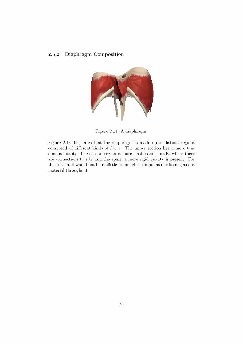
Figure 2.13: A diaphragm.

Figure 2.13 illustrates that the diaphragm is made up of distinct regionscomposed of di!erent kinds of fibres. The upper section has a more ten-donous quality. The central region is more elastic and, finally, where thereare connections to ribs and the spine, a more rigid quality is present. Forthis reason, it would not be realistic to model the organ as one homogeneousmaterial throughout.

20

Chapter 3

Biomechanical Modelling

Vital to any physical simulation is a solid understanding of the dynamics anda logical set of heuristic choices. This chapter assumes that a mass springsystem has been created which enforces the constraints of tensegrity. Thischapter will present the approximations and algorithms which have beenimplemented to match the motion of the diaphragm as closely as possible.

3.1 Diaphragm Mechanics and Tensegrity

As discussed in section 2.5.2, the nature of the diaphragm demands the useof di!erent materials to simulate its motion accurately. Tensegrity seemeda pertinent match that would be worthy of investigation.

A decision was made that the upper tendenous section of the organ wouldbe modelled using a combination of mass spring and tensegrity. The centralregion would be solely mass spring. Finally, the connections to the ribsand spine would be simulated using techniques described in ‘Fixed Points’,section 3.3. This division is visualised in figure 3.1 and the simulator’sresulting sections are in figure 3.2.

21

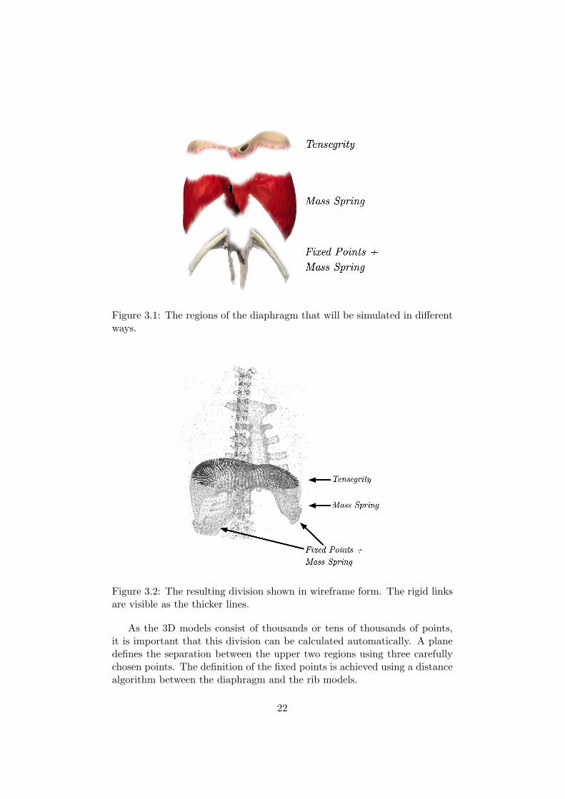
Figure 3.1: The regions of the diaphragm that will be simulated in di!erentways.

Figure 3.2: The resulting division shown in wireframe form. The rigid linksare visible as the thicker lines.

As the 3D models consist of thousands or tens of thousands of points,it is important that this division can be calculated automatically. A planedefines the separation between the upper two regions using three carefullychosen points. The definition of the fixed points is achieved using a distancealgorithm between the diaphragm and the rib models.

22

3.2 Rigid Connections

Figure 3.3: A cross-section of the desired result of the algorithm presentedhere.

Figure 3.3 shows two surfaces in close proximity with vertices representedby the circles. It would be ideal if the vertices directly opposite each otherwere connected via a rigid link, shown here by the thicker red line. Thedotted line represents the separation between the tensegrity and tensile partof the organ. In the final version of the application this separation is definedby a simple plane.

The reasoning behind the heuristic algorithm is as follows. Once a suit-able distance d has been chosen, a list of close masses is found. Thesemasses could either be neighbouring masses on the same surface or ideallythose on opposing surfaces. Testing the angle should remove those on thesame surface, leaving a sorted list of masses on the opposing surface.

This algorithm is performed once upon the initialisation of the simula-tion.

23

1 foreach(Mass v) {

2 Assemble a sorted list of other vertices within distance d.

3 }

4 foreach(Mass v) {

5 foreach(Mass o in v.closelist) {

6 Rem o from list if $ between normal at surfaces of o and v is acute.

7 }

8 }

9 foreach(Mass v) {

10 while(v.closelist is not empty & v has no rigid link) {

11 Pop o from v.closelist

12 if (o has no rigidlink & both lie above defining plane) {

13 Create rigid link between o and v, break.

14 }

15 }

16 }

Figure 3.4: Pseudocode of the rigid link creation algorithm.

Shown in figure 3.5 are the results of applying the algorithm in figure 3.4.The connections between the layers of the diaphragm appear to match veryclosely the desired result desribed at the start of this section(figure 3.3). Thetwo layers are heavily connected above the division between tensegrity andmass spring. The connections appear to be roughly at the opposite point,the aim of the algorithm.

24

Figure 3.5: The connections created between the layers of the diaphragm.

3.3 Fixed Points

Figure 3.6: A diagram of how points on the diaphragm are transformedrelative to rib motion. The length of the arrow is proportional to magnitude.The fall o! is visible in the centre displaced mass, M, compared to A and B.X and Y are located out of range of all the rib masses regions’ of influence.

At certain points the diaphragm is attached to the ribs. It is necessaryto mimic this connection in order for the motion to be realistic. Another

25

heuristic method was devised to fit this situation. Figure 3.6 helps to explainhow this is achieved. Firstly, pre-processing occurs in which each node inthe diaphragm is checked for proximity to a rib within a cut o! point. Ifthere are multiple choices, the closest is chosen. Then, a fall-o! factor isdetermined using 1! d

radius . At each iteration, the distance covered by eachnode in the ribs is calculated. A scaled value of this is applied to eachattached node multiplied by the fall o!. This gives the desirable result thatclose masses are influenced more and those further away will also move butwith less impetus. The corresponding pseudocode for these two steps isshown below.

1 Initialisation

2 foreach(Mass v in ribs) {

3 foreach(Mass m in diaphragm) {

4 Distance d = distance(v,m)

5 if (d < radius) {

6 m.addToCloseList(v,1! dradius)

7 }

8 }

9 }

Figure 3.7: Pseudocode for initialisation of fixed points.

1 Update code

2 foreach(Mass m in ribs.stuckmasses) {

3 Mass closest = m.closestnode;

4 Vector v = closest.getChangeInLocation();

5 m.applyForce(v*scalingfator);

6 }

Figure 3.8: Pseudocode run at each iteration to update the location of thefixed points.

26

3.4 Action Lines

Action lines are the simulation’s equivalent to muscle motion. Success hadbeen observed in the work of Nedel and Thalmann[NT] and an attempt tointegrate a similar e!ect was made. Figure 3.9 gives an intuitive look atthe approach adopted. In order to get an understanding of how the methodworks, it is best to imagine an infinitely long cylinder defined by a point, adirection vector and a fallo! radius. Pre-processing then occurs to find allmasses that fall within the fall o! range of the cylinder, based on the closest[perpendicular] distance to the central vector (shown by d in the figure).

At each iteration, a scaled value of the vector defining the direction ofthe cylinder is applied to each mass after being multiplied by verticaldistance

radiusThis means that the further away the point is, the stronger it feels the pull.This is a heuristic judgement of fall o!, but proved to be the most realisticof the various alternatives trialed.

Figure 3.9: A diagram showing the basic workings of the action line methodof imitating muscles.

27

3.5 Rib Kinematics

Another factor that plays a large role in respiration and the motion of thediaphragm is rib kinematics. Much of the work in this area was based onthat presented in [DV]. Figure 3.10 shows a spine and three ribs and helps toexplain how the rotations and displacements are calculated. In this project,existing C++ code implementing the rib kinematics was ported to Java.

The aim of the algorithm was to have a blend between vertical and lateralmotion of the ribs. The lower ribs ‘open’ up more during deep breathing,while the upper ribs have a more directly upward translation.

For a more in depth discussion of this process look at the work of Didieret al[DV].

tki = k (Ti) (3.1)ak

i = k (Ai) (3.2)i " [1, 20] (3.3)

Figure 3.10: A diagram showing the layout of the variable in equations 3.1-3.3.

28

Chapter 4

Implementation

Once initial research and information gathering had been completed, theimplementation stage of the project began with a focus on a SOFA basedsolution before migrating towards a custom Java solution for reasons to bediscussed.

4.1 SOFA Solution

The initial goal was to create a SOFA simulation that allowed the integrationof tensegrity as a forcefield. This would be highly desirable as SOFA isa framework designed for medical simulation. Its plug-and-play structurewould make the code reusable even as SOFA was updated in the future. Itwas also envisaged that a control panel would be added to allow the tuningof parameters controlling breath length, force and rib motion.

4.1.1 Background

SOFA aims to simplify the simulation of physical and, more specifically,medical simulations, by allowing the user to focus on the mechanics andtuning of the simulation, rather than the implementation and routine al-gorithms for displaying, mapping and solving systems. SOFA is written inC++ and currently contains 250,000 lines of code written by twenty devel-opers. The project benefited from the help of the CIMIT Sim Group, INRIAand ETH Zurich.

‘SOFA is an Open Source framework primarily targeted at real-time simulation, with an emphasis on medical simulation. Itis mostly intended for the research community to help developnewer algorithms, but can also be used as an e"cient prototypingtool. Based on an advanced software architecture, it allows to:

29

• Create complex and evolving simulations by combining newalgorithms with algorithms already included in SOFA.

• Modify most parameters of the simulation – deformable be-havior, surface representation, solver, constraints, collisionalgorithm, etc. – by simply editing an XML file.

• Build complex models from simpler ones using a scene-graph description.

• E"ciently simulate the dynamics of interacting objects us-ing abstract equation solvers

• Reuse and easily compare a variety of available methods

SOFA is currently developed by 3 INRIA teams: Alcove, Evasionand Asclepios.’

The SOFA Architecture [SOFA]

4.1.2 Diaphragm Motion in SOFA

Development

The work began as an introduction to medical simulation and consistedmainly in experimentation with parameters and di!erent models. It tooktime to become accustomed to features such as mapping between visual rep-resentations and the supporting mathematical simulation. This allows thevisual representation to be highly complex while reading its displacementsfrom a simplified underlying geometry. A diaphragm modelled by the finiteelement method is shown in figure 4.1. The associated XML file is shown infigure 4.2. The simulation uses a timestep of 0.02 seconds, uniform massesthroughout. Each object is fixed by three points and a simple static solveris used.

30

Figure 4.1: A diaphragm in SOFA, the tree of the scenegraph is visible onthe left.

31

Figure 4.2: An XML scenegraph describing two objects, a liver and a di-aphragm, both simulated using the finite element method.

<Node name="root" dt="0.02" showBehaviorModels="1" showCollisionModels="1"showMappings="0" showForceFields="1"><Object type="CollisionPipeline" verbose="0" /><Object type="BruteForceDetection" name="N2" /><Object type="CollisionResponse" response="default" /><Node>

<Object type="StaticSolver" name="solver" iterations="25" /><Object type="MechanicalObject" name="diaphragm" /><Object type="UniformMass" name="mass" mass="0.1" /><Object type="Mesh" filename="Topology/diaphragm.msh"/><Object type="Triangle"/><Object type="TriangleFEMForceField" name="FEM" youngModulus="5000"poissonRatio="0.3" />

<Object type="FixedConstraint" indices="3 39 64" /></Node><Node>

<Object type="StaticSolver" name="solver" iterations="25" /><Object type="MechanicalObject" name="liver" /><Object type="UniformMass" name="mass" mass="0.1" /><Object type="Mesh" filename="Topology/liver.msh" /><Object type="Triangle" /><Object type="TriangleFEMForceField" name="FEM" youngModulus="5000"poissonRatio="0.3" />

<Object type="FixedConstraint" indices="3 39 64" /></Node>

</Node>

Results

The results that were shown by SOFA were acceptable (15-20 iterations persecond) on a simple diaphragm model. It was during this initial testing thatthe issues discussed in 4.1.3 became apparent and forced a change in thedevelopment platform used in the project.

4.1.3 Issues with Heterogenity

After research into the possibilities of combing two simulation methods,FEM and mass spring, an issue within SOFA arose. In the current imple-mentation, mixing two force fields on one object is not possible. This was aserious problem as the aim was that parts of the diaphragm be modelled by

32

a simple mass-spring system and the rest with tensegrity. After consultingwith the developers of SOFA, they deemed it very di"cult to do this in thecurrent codebase. It was indicated that such a mix and match approachmay be available in future iterations, but no definitive time scale was given.

4.2 Java Solution

Forced to consider alternatives, the choice was then to proceed by makinga simple 2D simulator. This simulator could then be used to study theviability of a 3D implementation. Java fit the requirements of flexibility,cross-platform nature, and prior familiarity and as such was chosen as themain language for the simulator. An iterative scheme fits well with thedevelopment plan of the project. It was first decided to concentrate onsimple structures with few nodes in 2D before considering expansion into3D. Once the transition to 3D was made, parsers of file formats, exportersand other options were added.

4.2.1 Basic Class Structure

Once development had begun, a modular design was necessary to keep flex-ibility for future additions to the design and functionality. The end resultis a relatively concise, but productive set of classes to provide real-time in-teraction. There are packages to handle the importing and exporting ofdata, mathematical classes, model classes and those that aid in the anima-tion and motion of the ribs. Another software-engineering decision was thecreation of an abstract simulator class which is then extended upon for eachindividual situation. This is shown in figure 4.3.

33

Figure 4.3: A simplified UML diagram of the Simulator class hierarchy.

4.2.2 2D Display

The initial 2D display was just a case of plotting some points and updatingthis graph to provide animation(figure 4.4). A generic graphing package waschosen for this purpose, JFreeChart1. It gave a simple method of updat-ing and displaying charts on screen. This allowed the focus to be on themathematics and correctness of the data, rather than on the mechanics ofdisplaying it.

A simple point plot was chosen as it allowed the fastest developmenttime and gave a quick mapping between the data behind the simulationand a visual representation. There are issues with flicker as a result ofthe continuous updating of the point locations but this is acceptable as theapplication was meant as more of a proof of concept.

1http://www.jfree.org/jfreechart/

34

Figure 4.4: An annotated diagram, thin green and thicker red lines representtensile and rigid connections respectively.

4.2.3 3D Display

Once the solving of systems involving tensegrity had been shown to be possi-ble in real time and of possible interest in tissue simulation, the decision wastaken to develop a 3D visualisation. Several options were available here, butthe decision was taken to use the Java3D library2 as it is a mature codebasewith low-level driver integration. The fact that the intensive code is nativeand not part of the Java Virtual Machine means that it is much more likelyto give high performance in more strenuous circumstances.

Initially, only simple nodes and connections were represented withoutfaces. Later on, support for shading, lighting, textures and specularity wereadded. A simple box simulation was created and manipulated by randomforces to test the behaviour of the system and check for realism(figure 4.5).

2http://java.sun.com/products/java-media/3D/

35

Figure 4.5: An early 3D version of the simulator with a basic tensegritysituation.

Changes Required

The conversion from 2D to 3D was not that involved as a result of the highcohesion within the classes. The majority of modifications were made inthe vector and display classes. An extra component needed to be createdand taken into account in such calculations as distance metrics. The displayneeded to feed the updated points to Java3D, which at first were set on anindividual basis.

Exporting the result

In a medical simulation, verification and validation are a crucial aspect ofthe application. Even if the system looks to be performing correctly, it isimperative that there is a way to export data that can be inspected usingother software. Gmsh3 was selected as a tool which provided the function-ality required for visual verification of diaphragm and rib deformation.

The ‘.depl’ format was cumbersome to implement. Its layout is shownin table 4.1. Header information alerts the parser to the kind of shapedata incoming and the number of vertices. After the initial location hasbeen stored, the change in x, y and z on a vertex by vertex basis fromthe previous iteration is required at each timestep. In systems with tens ofthousands of vertices, storing this amount of data can become a strain onmemory of the machine.

3http://www.geuz.org/gmsh/

36

Table 4.1: ‘Depl’ file format showing basic structure. The file is then flat-tened, preserving the newlines shown below.

Vertex Timestep X Y Z1 tinitial 5 10 5

t1 0.9 0.4 0.1t2 0.31 0.25 0.2t3 0.4 0.1 0.3...

......

...tn tn(x)! tn"1(x) tn(y)! tn"1(y) tn(z)! tn"1(z)

2 tinitial 2 -6 18t1 0.0 0.0 0.1t2 0.5 0.3 0.2t3 -0.17 -0.1 -0.2...

......

...tn tn(x)! tn"1(x) tn(y)! tn"1(y) tn(z)! tn"1(z)

......

......

...

Optimisations

Once the system had been converted to 3D, it became possible to repre-sent structures within the human body. These were provided in ‘.msh’ fileswhich could be parsed using a custom built package. Once this had beencompleted, it was then possible to simulate the mass spring system usinga large scale simulation. The results were not adequate as one frame wasdrawn every thirty seconds or more. After investigation, it became apparentthat the bottleneck was the copying of data between the internal Java3Drepresentation of the scene and that held in the model of the simulation. Tosolve this problem, Java supports another paradigm to update geometries.It allows a geometry to be passed as an array of floats. This array mustbe 1-dimensional, which reduces code-readability as o!sets and multipliersmust be used for access; this is necessary if higher speed is a requirement.It is then just a case of alerting the Java3D classes that changes have beenmade. This allowed the full scale simulations to run in real time thereforemaking tuning an option.

4.3 The Final Product

At the completion of the project, a fully-tunable simulation system wascreated with four options available. Two involving simple cubes to see thee!ect of tensegrity, one of a ‘perfectly’ modelled diaphragm and one from CT

37

scans (shown in figures 4.6). The control panel used to tune the simulationin real time can be seen in figure 4.7.

Figure 4.6: Images from the completed simulator. Left: The simulator usingthe ‘perfect’ model. Right: The result of using the data from the CT scan.

Figure 4.7: The final control panel for the ‘perfect’ simulator.

38

Where:Timestep: The parameter used in the Euler solver.Breath Force: Controls the force of the action lines, see figure 4.8and equation 4.1.Breath Length: Sets the length of each breath, see figure 4.8 andequation 4.1.Rib Motion: Modifies the angle by which the ribs rotate.Elasticity : A parameter of the mass spring system.Transparency : Used to show or hide the shaded faces.Apply Muscles: Activates or deactivates the action lines.Show etc.: Visual options

Figure 4.8: Illustrating the breathing motion.

y = C1(BreathForce)sin,

C2T

BreathLength

-(4.1)

C1 and C2 are two constants chosen to make the values of Breath Forceand Breath Length scale to interesting values for each simulation. T is thetime elapsed in the simulation.

39

Chapter 5

Evaluation

The Java implementation presented in the previous sections will now bequantitatively and qualitatively evaluated along with the influence of tenseg-rity.

5.1 Tensegrity

One of the main purposes of this project was to evaluate the viability oftensegrity for simulating the tendonous tissue of the diaphragm. This is nota trivial task and a few di!erent methods were used to test this.

Firstly, it was decided to have a test to see if tensegrity did indeed providemore support than a typical mass spring system. This was tested using asimple cube as shown in figure 5.1. The‘ cube was created with diagonalrigid supports between the upper and lower levels.

Figure 5.1: The standard tensegrity cube that was used in the initial eval-uation of the e!ects of tensegrity.

Two points on the upper square were then manipulated by applying asinusoidal motion. The data was exported and visually analysed. It was

40

obvious that the mass spring system collapses in on itself with much lowerforces, while the tensegrity solution is able to maintain its shape. The resultsare shown in figures 5.2 and 5.3.

YXZ

PF

F

-30-20-10

0 10 20 30

0 500 1000 1500 2000

F [N

]Time [ms]

A force is applied to two nodes: positive along the X axis, negative along theY axis and has an intensity given by a sinusoid curve

time=66% of the period time=76% of the period time=81% of the periodBehaviour of the cube with a mass spring system.

time=66% of the period time=76% of the period time=81% of the periodBehaviour of the cube with tensegrity.

Figure 5.2: Cube (10 # 10 # 10m3) evolution with time. Top: boundaryconditions, Middle: results with a mass spring system, Bottom: results withtensegrity

41

-9-8-7-6-5-4-3-2-1 0 1

0 500 1000 1500 2000

Y Di

spla

cem

ent [

m]

Time [ms]

-0.07-0.06-0.05-0.04-0.03-0.02-0.01

0

0 500 1000 1500 2000

Y Di

spla

cem

ent [

m]

Time [ms]

Figure 5.3: Y-value of a mass p in figure 5.2. The mass spring system is onthe left, tensegrity on the right. The tensegrity is system able to absorb thepressure and rebound, the mass spring collapses.

5.1.1 E!ect on Diaphragm

Figures 5.5 and 5.6 quantify the e!ect of tensegrity. The data for the graphswas extracted as follows:

1. A point on the top of the diaphragm was chosen, illustrated by fig-ure 5.4.

Figure 5.4: The chosen node was within the region shown.

2. 200 iterations were performed and the location of the chosen point wassaved each time.

3. This simulation was performed with and without rigid links and thevalues were then subtracted to produce the data. The y-axis waschosen to be plotted as it is the main direction of translation in thediaphragm.

In figure 5.5 the di!erence is small initially and steadily rises. This couldimply that there is just noise that is slowly being accumulated. It could alsoimply that the forces are not strong enough to require the rigid constraint.

42

Figure 5.6 provides a more interesting situation. In this case the forceswere multiplied by a factor of 10. The di!erence between the values isno longer a steadily increasing function. There are abrupt troughs andhills as the constraints of tensegrity are applied. This shows that in morestrenuous circumstances tensegrity can be used to enforce the proximity ofthe opposing sides of the diaphragm.

]

0

0.002

0.004

0.006

0.008

0.01

0.012

0.014

1 51 101 151

Disp

lace

men

t D

i!er

ence

Iteration

!"

!#$"

%"

%#$"

&"

&#$"

'"

'#$"

%"

%%"

&%"

'%"

(%"

$%"

)%"

*%"

+%"

,%"

%!%"

%%%"

%&%"

%'%"

%(%"

%$%"

%)%"

%*%"

%+%"

%,%"

-./0.1%"

-./0.1&"

Figure 5.5: A plot of the di!erence between the y-component of the chosenpoint with and without rigid links. Weak action line forces were applied.

]

0

0.02

0.04

0.06

0.08

0.1

0.12

0.14

0.16

1 51 101 151

Disp

lace

men

t D

i!er

ence

Iteration

!"#

!$#

!%#

!&#

'#

&#

%#

$#

"#

('#

(&#

(#

((#

&(#

)(#

%(#

*(#

$(#

+(#

"(#

,(#

('(#

(((#

(&(#

()(#

(%(#

(*(#

($(#

(+(#

("(#

(,(#

-./0.1(#

-./0.1&#

Figure 5.6: A plot of the di!erence between the y-component of the chosenpoint with and without rigid links. Strong action line forces were applied.

43

5.2 Diaphragm Motion

The ‘Perfect’ Model

Figure 5.7: The resulting motion during the simulation.

The favourable results observed in the simple simulation were encouragingand the task of analysing the realism of tensegrity in diaphragm was tofollow. For the so called ’perfect’ model, a commercially available referencemodel of the diaphragm was used. It consisted of 11359 vertices and 22722triangles. It can be very di"cult to verify the realism of the motion in sucha large model.

The wireframe visible in 5.7 represents the initial state at the end of aninhale. The coloured geometry represents the diaphragm at the end of anexhale. The upper region has kept its shape due to the tensegrity while thelower region has been more deformed as it had no rigid links to help retainits shape.

The three sources of motion on the diaphragm are visible here:

• Muscle Motion: The muscle relaxation that increases the height of thedomes is visible.

• Rib Kinematics: On the sides of the diaphragm the motion as a resultof the rib kinematics is visible.

• Sternum Motion: In the central front region the e!ect of the sternumis also visible as it influences the tissue to which it is connected.

Verification was also made by a clinical collaborator who validated themotion and also explained how only the diaphragm’s domes descend duringlight breathing. The tuning options provided by the control panel mean sucha situation is easily simulated. Under heavier breathing, the diaphragm canmove substantially and this is also possible to recreate.

44

5.2.1 The Patient Model

Verification of the patient model was achieved using data from a 4D CTscan. The diaphragm was segmented and smoothed. This process is shownin 5.8. The resulting diaphragm mesh is composed of 20740 vertices and41480 triangles.

Figure 5.8: Left: Segmented diaphragm inside CT scan and right: Combi-nation of segmentation and the mesh, the smoothing is visible on the right.

The simulation was validated by comparing the results of the simulationto the 4D CT scan data at the same point in the breathing cycle. The exportfunction of the simulation software was used. The CT scan data was usedfor the real patient. The distance between the two were studied using theMESH1 software to analyse meshes. It then found the Hausdor! distance2.The results of the analysis are visible in figure 5.9. By visual inspection, clearsimilarities are present in several regions. The correspondence appears tobe relatively close, but inaccurate in terms of magnitude in certain regions.This led to the conclusion that the tuned simulation mirrors this patient’strue breathing pattern e!ectively.

5.3 Simulator

The tests below were performed on a dual core 2.4 ghz machine with 2gigabytes of ram and a 256 megabyte graphics card. The operating systemwas Windows Vista Service Pack 1 with Java 1.6 installed. The parametersof the simulation were on their default values. All results are in secondsunless otherwise stated.

1http://mesh.berlios.de/2The Hausdor! distance between two sets of points is the longest distance an adversary

can force you to travel by choosing a point in one of the two sets, from where you thenmust travel to the other set.

45

Figure 5.9: Distance error measurement between left: beginning and end ofreal inhale and right: simulated end of inhale and real end of inhale.

5.3.1 Cube Simulation

To test the cube simulation and the influence of tensegrity on simulationperformance, 100,000 iterations were performed and the two cubes withsinusoid forces being applied.

Figure 5.10: Cube simulation performance (in seconds).Tensegrity Tensile

Simulated Vertices 8 8Trial 1 4.174 3.155Trial 2 4.287 3.337Trial 3 4.069 3.602Trial 4 4.599 3.244Trial 5 4.198 3.387

Average 4.2654 3.345

0s

5s

10s

15s

20s

25s

Tensegrity Tensile

Chart 13

Figure 5.11: A graphical representation of the results, each colour representsa separate trial.

Tensegrity TensileSimulated Vertices 8 8

Trial 1 4.174 3.155Trial 2 4.287 3.337Trial 3 4.069 3.602Trial 4 4.599 3.244Trial 5 4.198 3.387

Average 4.2654 3.345

0s

5s

10s

15s

20s

25s

Tensegrity Tensile

Chart 13

46

It can be seen from the graph that the addition of the tensegrity con-straint makes for a slightly slower simulation, but it is still more that ad-equately fast. The use of tensegrity shows a computational cost of 27%.This cost is o!set by the desirable strength that the rigid links provide asdiscussed in section 5.1.

5.3.2 Diaphragm Simulation

Now that the realism of the simulations have been evaluated it is time toverify the computational cost of the simulation parameters. Two cases weretested for the perfect simulator. In one case, the fixed points were no longercalculated and adjusted at each iteration. The other variation was the re-moval of rib kinematics.

Figure 5.12: Diaphragm simulation performance (in seconds).Full No Rib/Sternum Attachment No Rib Kinematics

Simulated Vertices 20740 20859 11359Trial 1 15.472 12.174 12.256Trial 2 15.39 12.098 12.097Trial 3 15.448 12.126 12.043Trial 4 15.654 12.565 12.129Trial 5 15.435 12.534 12.261

Average 15.4798 12.2994 12.1572

0s

20s

40s

60s

80s

Full No Rib/Sternum Attachment No Rib Kinematics

Chart 1Figure 5.13: A graphical representation of the results, each colour representsa separate trial.

Full No Rib/Sternum Attachment No Rib KinematicsSimulated Vertices 20740 20859 11359

Trial 1 15.472 12.174 12.256Trial 2 15.39 12.098 12.097Trial 3 15.448 12.126 12.043Trial 4 15.654 12.565 12.129Trial 5 15.435 12.534 12.261

Average 15.4798 12.2994 12.1572

0s

20s

40s

60s

80s

Full No Rib/Sternum Attachment No Rib Kinematics

Chart 1

It can be seen that the slowest simulator is the ‘real’ simulator. This canbe attributed to the high count of vertices involved in the simulation. The‘perfect’ simulator is slightly faster and the variations do make a di!erenceto the speed of calculation. Rib kinematics make a considerable di!erenceto the speed. This is a result of some large equations being solved to updatethe locations at each iteration. If a patient is observed to only be using the

47

diaphragm and no rib action during respiration, a large computational costcan be avoided.

5.3.3 Influence of Mesh Size with a Heterogeneous Model

Another influencing factor on the speed of a simulation is the size of themesh. Both the ‘perfect’ and patient models were tested with di!erentresolutions.

Figure 5.14: The timed results of the perfect mesh being resized.High Medium Low


Average 12.2994 9.6106 7.8196

0s

17.5s

35.0s

52.5s

70.0s

High Medium Low

Chart 1Figure 5.15: The perfect mesh times.

High Medium LowSimulated Vertices 20909 16023 12047


Average 12.2994 9.6106 7.8196

0s

17.5s

35.0s

52.5s

70.0s

High Medium Low

Chart 1

Figure 5.16: The timed results of the patient mesh being resized.High Medium Low


Average 15.7004 8.3012 5.1564

0s

20s

40s

60s

80s

High Medium Low

Chart 148

Figure 5.17: A graph of the patient data.



Average 15.7004 8.3012 5.1564

0s

20s

40s

60s

80s

High Medium Low

Chart 1

A quick look at figures 5.14-5.17 shows an intuitive linear relationshipbetween the number of vertices in the scene and the time taken in compu-tation. Figure 5.18 shows this relationship in the patient data case.

Figure 5.18: A graph of simulation time against the vertices in the hetero-geneous patient simulator.

Vertices

Trial 1 Trial 2 Trial 3

Vertices 20740 10162 5185

Time vs. Vertices 15.7004 8.3012 5.1564

0 2 4 6 8

10 12 14 16 18

0 5000 10000 15000 20000 25000

Tim

e

Vertices

5.3.4 Influence of Mesh Size with a Homogenous Model

Similar to section 5.3.3 the mesh sizes were reduced in complexity and thentests were conducted without rigid links, creating a standard mass springmodel.

49

Figure 5.19: The timed results of the perfect mesh being resized.High Medium Low


Average 11.6868 9.3574 7.6508

0s

15s

30s

45s

60s

High Medium Low

Chart 1Figure 5.20: The perfect mesh times.



Average 11.6868 9.3574 7.6508

0s

15s

30s

45s

60s

High Medium Low

Chart 1

Figure 5.21: The timed results of the patient mesh being resized.High Medium Low


Average 14.6198 7.9392 5.0788

0s

20s

40s

60s

80s

High Medium Low

Chart 1

50

Figure 5.22: A graph of the patient data.



Average 14.6198 7.9392 5.0788

0s

20s

40s

60s

80s

High Medium Low

Chart 1

As seen in figures 5.19-5.22 the recorded times were very similar to thosewith tensegrity and were only o! by a small percentage. This demonstratesthat even in large models with hundreds of rigid links, the computationaltime is not massively increased. The linear relationship between verticesand time still holds as shown in figure 5.23.

Figure 5.23: A graph of simulation time against the vertices in the homoge-nous patient simulator.

Vertices

Trial 1 Trial 2 Trial 3

Vertices 20740 10162 5185

Time vs. Vertices 14.6198 7.9392 5.0788

0

2

4

6

8

10

12

14

16

0 5000 10000 15000 20000 25000

Tim

e

Vertices

5.3.5 Conclusions

After many tests, table 5.24 provides a succinct summary of all the data.It gives the average iterations per second after five trials. The relationshipbetween the parameters of the simulation and the mesh size are availablehere, but are better visualised in figures 5.25 and 5.26. Figure 5.25 showsmore interesting behaviour. The computational time of the rib kinematics is

51

shown to be quite high as when they are removed in the ‘Action Lines Only’trial the simulation hits its peak. Figure 5.26 is a fairly intuitive graph thatshows an inverse relationship between model complexity and iterations persecond.

Figure 5.24: A summary of the iterations per second of all the simulations.The trials have been averaged into a single value.

Perfect ModelVertices Heterogenous

Model (All Forces)Homogenous

Model (All Forces)Rib Kinematics Only

(Heterogenous)Diaphragm

Contraction/Relaxation Only (Heterogenous)

asdfasdf Iterations

High 20909 8.13 8.56 8.24 9.68 100

Medium 16023 10.41 10.69 10.93 11.76Low 12047 12.79 13.07 13.27 14.70

Patient ModelVertices Heterogenous

Model (All Forces)Homogenous

Model (All Forces)High 20740 6.37 6.84

Medium 10162 12.05 12.60Low 5185 19.39 19.69

12.174 11.542 12.140 10.477 15.931 14.522

12.098 11.831 11.931 10.272 15.386 14.865

12.126 11.732 11.651 10.359 15.778 14.469

12.565 11.657 12.235 10.308 15.659 14.629

12.534 11.672 12.748 10.258 15.748 14.614

9.543 9.703 9.191 8.543 8.597 7.839

9.630 9.206 9.310 8.103 8.313 7.929

9.552 9.144 8.816 9.020 8.077 7.920

9.725 9.043 9.345 8.643 8.500 8.016

9.603 9.691 9.103 8.211 8.018 7.992

7.851 7.832 7.011 6.554 5.167 5.063

7.735 7.645 7.843 6.842 5.092 5.047

7.907 7.451 7.861 7.050 5.217 4.983

7.842 7.621 7.412 6.612 5.081 5.087

7.763 7.705 7.565 6.945 5.225 5.214

Figure 5.25: A 3D plot of the iterations per section of the ‘perfect’ simula-tion. The axes are: simulation parameters, mesh quality, and iterations persecond.

High Medium

Low 8

10

12

14

16

Diap

hrag

m C

ontr

actio

n/Re

laxa

tion

Onl

y (H

eter

ogen

ous)

Rib

Kin

emat

ics O

nly

(Het

erog

enou

s)

Hom

ogen

ous M

odel

Hete

roge

nous

Mod

el

14-16 12-14 10-12 8-10

52

Figure 5.26: A 3D plot of the iterations per section of the patient simula-tion. The axes are: simulation parameters, mesh quality, and iterations persecond.

High

Medium

Low

6

10

14

18

22

Heterogenous Model (All Forces)

Homogenous Model (All Forces)

18-22 14-18 10-14 6-10

Computational Cost of Tensegrity on Simulations

Figure 5.27 shows the cost on the speed of the simulator that the additionof tensegrity makes. The largest change is visible in the high quality perfectmodel. This is due to the very high number of connections created in thiscase. The overall cost of the tensegrity connections is seen to be relativelylow.

Figure 5.27: The percentage change in each of the simulations.Perfect Model

Vertices Tensegrity Mass Spring Rigid Links: Vertices Ratio

Percentage Change

Iterations

High 20909 8.13 8.56 1663:20909 5.24% 100

Medium 16023 10.41 10.69 1022:16023 2.71%Low 12047 12.79 13.07 602:12047 2.21%

Patient ModelVertices Tensegrity Mass Spring Rigid Links:

Vertices RatioPercentage

ChangeHigh 20740 10.40 10.78 4858:20740 3.65%

Medium 10162 10.41 10.69 648:10162 2.71%Low 5185 10.39 10.79 940:5185 3.85%

12.174 11.542 15.931 14.522

12.098 11.831 15.386 14.865

12.126 11.732 15.778 14.469

12.565 11.657 15.659 14.629

12.534 11.672 15.748 14.614

9.543 9.703 8.597 7.839

9.630 9.206 8.313 7.929

9.552 9.144 8.077 7.920

9.725 9.043 8.500 8.016

9.603 9.691 8.018 7.992

7.851 7.832 5.167 5.063

7.735 7.645 5.092 5.047

7.907 7.451 5.217 4.983

7.842 7.621 5.081 5.087

7.763 7.705 5.225 5.214

53

Chapter 6

Conclusion

6.1 Discussion

6.1.1 Work Completed

By the end of the project, a tuneable simulator capable of simulating tissueswithin the body was created. It receives input in the form of mesh files andrigid links are created automatically once a plane has been defined. Muscleaction is simulated through action lines. After initialisation, the simulationis controlled via a panel containing parameters such as breath length, forceand rib motion. These parameters allow the simulation to match closely apatient’s breathing pattern. Finally, an analysis and evaluation was con-ducted to investigate the e!ectiveness and computational cost of tensegrity.

6.1.2 Project Outcomes

The result is a code base that is malleable to future modifications to fit otherpurposes. It can be seen through the background work that the diaphragmis composed of materials of various properties and heterogeneity is neededfor a true simulation of diaphragm motion. Tensegrity can be shown toprovided additional support in structures(figure 5.2). Verification of realismwas adequate but, for an organ with so many influencing factors, moreevaluation is required.

6.1.3 Limitations

At the current time, although the design is very tuned to the purpose ofsimulating the diaphragm, some minor work would be required to modify itto a more generic form. There are also several other useful paradigms thatSOFA has that could be desirable here. Mapping between a visual modeland a mechanical backing would allow the simulation to take place at a lowerlevel and the visual model to be of a much higher quality. Finally, probably

54

the largest limitation is the lack of interchangeability of simulation methods.If the project had been completed wholly in SOFA, other tissue simulationmethods could quickly be substituted for easy comparison.

6.2 Future work

The project had a large research aspect to it and therefore there is plentyof scope for future work.

6.2.1 Integration with SOFA

Now that the use of tensegrity has been found to be valid and worth im-plementing, it would be ideal to integrate it into SOFA. Creating a systemof mixing mass spring and rigid links could be completed in the currentversion of SOFA. For the potential mixing of rigid and the finite elementmethod, a newer version of SOFA with the combination of force fields wouldbe required.

6.2.2 Educational Context

Once a more thorough and complete evaluation has been completed and anymodifications made, the tool could be used to give an insight into the motionof the diaphragm during di!erent kinds of breathing. The results should beenough to give the correct impression and coupled with the interactivity andvisible combination of forces, it could prove to be an interesting teachingtool.

6.2.3 Haptic Integration

Haptic means pertaining to the sense of touch. In medical simulation, theuse of touch to give the impression of applying forces or the feeling of vi-bration adds a very strong element of realism. A future project could bethe integration of haptic elements to the simulator. Liver access is greatlycomplicated by the motion of the diaphragm and a haptic aspect of thesimulation could prove to be a valuable tool in training surgeons.

55

Bibliography

[AC] M.N. Acharya, “Modelling of Diaphragm Motion for Simulationof Liver Access”, Surgery and Anaesthesia BSc Project, ImperialCollege London, May 2008, Pages 13-14, 33-35.http://www1.imperial.ac.uk/resources/A7C4A779-D4F9-4527-90BC-6D5C1A6435BC/

[BL] Y. Bhasin, A. Liu, “Bounds for Damping that Guarantee Stability inMass-Spring Systems”, The Surgical Simulation Laboratorye, 2005,Pages 1-3.

http://simcen.org/pdf/bhasin%20mmvr%202006.pdf

[BW] D. Bara!, A. Witkin, “Large Steps in Cloth Simulation”, RoboticsInstitute, Carnegie Mellon University. Pages 1-5.

http://ai.stanford.edu/~latombe/cs99k/2000/cloth.pdf

[DV] A. Didier, P. Villard, J. Bayle, M. Beuve, B. Shariat, “BreathingThorax Simulation based on Pleura Physiology and Rib Kinematics”,Hopital Louis Pradel, Lyon, France, 2007, Pages 1-5.http://www710.univ-lyon1.fr/ mbeuve/pvillard/zurich07.pdf

[GU] A. Guillaume, “Simulation 3D du comportement biomecanique descellules”, Masters Thesis, Universite Claude Bernard Lyon I, 28 June2004, Pages 7-12.

[IN] D.E. Ingber, “Opposing views on tensegrity as a structural frameworkfor understanding cell mechanics”, Journal of Applied Physiology 89:1663-1678, 2000.

[ML] U. Meier, O. Lopez, C. Monserrat, M.C. Juan, M. Alcaniz, “Real-time deformable models for surgery simulation: a survey ”, ComputerMethods and Programs in Biomedicine (2005) 77, 183-197.

[NT] Nedel, Luciana Porcher & Thalmann, Daniel, “Real Time MuscleDeformations Using Mass-Spring Systems”, EPFL - Swiss FederalInstitute of Technology, Pages 2-11.

[SOFA] SOFA, Simulation Open Framework Architecture,http://www.sofa-framework.org/

56

[VB] F.P. Vidal, F. Bello, K.W. Brodlie, N.W. John, D. Gould,R. Phillips, N.J. Avis, “Principles and Applications of ComputerGraphics in Medicine”, Computer Graphics Forum, Volume 25, Num-ber 1, March 2006 , Pages 113-137.

57

Appendix A

Appendix

A.1 User Guidance

A.1.1 Adding a new object

1. Convert your model to ‘.msh’ format : Before importing a model itneeds to be converted into the correct format. A parser has beencreated that will do this for you and is included. It requires simple‘.obj’ models without textures or lighting.

2. Add Java3D and Topology variables: Java3D needs to have variablesto store the geometries you are going to be adding, these are declaredat the top of the simulator classes.

static Topology diaphragm = null;

TriangleArray diaphragmtriangles;Shape3D diaphragmshape;

3. Create an entry in init3D(): This method is where the Java3D pa-rameters of the display such as colour, specularity and material areset.

if (diaphragm != null) {Appearance app = new Appearance();

Material material = new Material();PolygonAttributes pAttr = new PolygonAttributes();

pAttr.setPolygonMode(PolygonAttributes.POLYGON_FILL);pAttr.setCullFace(PolygonAttributes.CULL_NONE);

58

pAttr.setBackFaceNormalFlip(false);

material.setShininess(128f);material.setDiffuseColor(1.0f,0.0f,0.0f);material.setAmbientColor(1.0f,0.0f,0.0f);

app.setMaterial(material);app.setPolygonAttributes(pAttr);

diaphragmtriangles = new TriangleArray(diaphragm.triangles.size()*3,GeometryArray.COORDINATES | GeometryArray.BY_REFERENCE |GeometryArray.NORMALS);diaphragmtriangles.setCapability(GeometryArray.ALLOW_REF_DATA_READ);diaphragmtriangles.setCapability(GeometryArray.ALLOW_REF_DATA_WRITE);diaphragmtriangles.setNormalRefFloat(diaphragm.normals);diaphragmtriangles.setCoordRefFloat(diaphragm.locations);

diaphragmshape = new Shape3D();diaphragmshape.setCapability(Shape3D.ALLOW_GEOMETRY_WRITE);diaphragmshape.setAppearance(app);diaphragmshape.addGeometry(diaphragmtriangles);transformGroup.addChild(diaphragmshape);

}

4. Parse file and setup connections in init(): The model needs to bebound to the diaphragm topology. Connections also need to be cre-ated.

MSHParser diaphragmparser = new MSHParser();diaphragm = new Topology("Diaphragm");

try {diaphragmparser.parseFile("diaphragm.msh",diaphragm,MSHParser.SETUPCONNECTIONS,-135);diaphragm.setupArrays();new ActionLine(diaphragm.nodes.get(9113).initialloc,new Vector(0.0f,1.0f,0.0f), 17.0f, new Vector(0.0f,0.2f,0.0f), diaphragm);new ActionLine(diaphragm.nodes.get(1557).initialloc,new Vector(0.0f,1.0f,0.0f), 14.0f, new Vector(0.0f,0.2f,0.0f), diaphragm);

} catch (Exception e) {System.out.println("Error parsing files");e.printStackTrace();return;

}

59

The MSHParser.SETUPCONNECTIONS tells the parser that you wouldlike the mass spring connections to be created for you. This may notbe desirable if you are going to be using this as a rigid structure, suchas the spine. In this case you should use MSHParser.NOCONNECTIONS.The !135 argument of the parseFile(...) call is a y-value scalar.This is used to centre the diaphragm as the model was o!-center. 0should be placed here if the model is already centred around the origin.

Actionlines are also created here with the form: new ActionLine(Origin,Direction Vector, Radius, Force Vector, Object);

5. [Optional] Create rigid links in init(): The topology can be told tocreate rigid links between its internal surfaces.

diaphragm.setupInternalConnections(3474,1994,636,1.5f);

The first three are the node numbers of the nodes to define the plane.The fourth argument is the maximum distance each node will consideras neighbours.

6. [Optional] Create attachments between objects in init(): The topol-ogy can be attached to other topologies to simulate connected tissues.

diaphragm.stickTo(sternum_ligaments, 0.5f,20f);diaphragm.resolveClosestEntries();

The first argument is the opposing tissue you wish to attach to, thesecond is the distance limit for neighbours and the third is a scalar forthe forces to be applied.

Finally, the computation to find closest node in the neighbouring topol-ogy is completed by diaphragm.resolveClosestEntries().

7. [Optional] Add references in toggleShaded(): The GUI allows shadedmodels to be hidden. A reference needs to be added here if you wantyour object to be hidden also.

public void toggleShaded() {if (diaphragmshape.numGeometries() > 0) {

diaphragmshape.removeAllGeometries();} else {

diaphragmshape.addGeometry(diaphragmtriangles);}

}

60

A.1.2 Action Line Fall O! Modication

The action line method is very amenable to tuning for a variety of situations.For this reason I will show the method that needs to be modified to performthe tuning.

public void applyForces(float scalingfactor) {for (Node n: nodes) {

float[] p = n.getLocation();Vector3f point = new Vector3f(p[0],p[1],p[2]);float distance = point.y-origin.y;float falloff = distance/radius;

if (falloff > 0 & n.force == null) {forcevector.Multiply(scalingfactor*falloff);n.addForce(forcevector.clone());forcevector.Divide(scalingfactor*falloff);

}}

}

As is visible here the fall o! is currently concerned with the ratio betweenthe di!erence of the y values of the point and the origin and the radius.Changing this fall o! calculation will provide vastly di!erent behaviour ofthe action line.

A.1.3 Euler Solver Implementation

The solver is another crucial aspect of the project that could be tuned toprovide better convergence or a faster simulation.

The simulator has the following code within the performIteration()method.

for(Node n: t.nodes) {Vector v = n.calculateTensionForces();n.applyForce(v);n.updateVelocity();n.updateDamping();n.updatePosition();

}

The tension forces are calculated using equation 2.1. applyForce(Vectorf) is defined as follows and is a simple application of Newton’s second law,f = ma.

61

public void applyForce(Vector f) {/* f = ma, a = f/m */if (!this.isFixed()) {

f.Divide(mass);acceleration = f;

} else {acceleration = new Vector(0,0,0);

}}

updateVelocity() is defined as:

public void updateVelocity() {acceleration.Multiply(Simulator.TIMESTEP);velocity = Vector.add(velocity, acceleration);

}

updateDamping() is defined as follows where dampingfactor is an experi-mentally chosen constant of !0.02.

public void updateDamping() {applyForce(Vector.Multiply(velocity, dampingfactor));velocity = Vector.add(velocity, acceleration);

}

Finally updatePosition():

public void updatePosition() {Vector distance = Vector.Multiply(velocity,Simulator.TIMESTEP);newloc.x += distance.x;newloc.y += distance.y;newloc.z += distance.z;

}

The numerical integration shown here is simple and quick to process. Othermethods such as Runge–Kutta could be used to provide a better solution.

62

The Use of Tensegrity to Simulate Diaphragm Motion Through ...

Documents

Transcript of The Use of Tensegrity to Simulate Diaphragm Motion Through ...