The Pennsylvania State University

The Graduate School

The Use of Adjoint Methods in Jet Nozzle Design

A Thesis in

Aerospace Engineering

by

Nidhi Sikarwar

© 2009 Nidhi Sikarwar

Submitted in Partial Fulfilment

of the Requirements

for the Degree of

Master of Science

December 2009

ii

The thesis of Nidhi Sikarwar was reviewed and approved∗ by the following:

Philip J. Morris

Boeing/A.D. Welliver Professor of Aerospace Engineering

Thesis Advisor

Dennis K. McLaughlin

Professor of Aerospace Engineering

George A. Lesieutre

Professor of Aerospace Engineering

Head of the Department of Aerospace Engineering

∗ Signatures are on the file in the Graduate School.

iii

Abstract

The use of adjoint methods for aerodynamic design has been a major topic of

research because of its benefits over traditional aerodynamic design. Traditional

aerodynamic design is performed by changing the geometry and solving the flow

equations for many possible geometries to see which one is the “optimum”

geometry. The geometry could be optimum on different bases. One is trying to

minimize or maximize a given objective function. This objective function may be the

drag or lift or some other property depending upon the problem. Adjoint methods

are used to find the direction of steepest descent by finding the gradients of the

objective function with respect to the design parameters. Direct calculation of these

gradients requires massive computational power, whereas solving the adjoint

equation costs the same computationally as solving the flow equation. Hence, the

use of adjoint methods saves on computational cost. In this thesis the use of adjoint

design methods is presented for the design of a jet nozzle contour. The design is

performed in such a manner that it gives a desired pressure distribution on the

nozzle centerline. Both supersonic and subsonic cases are considered to explain the

use of the adjoint method for design.

iv

Table of Contents

List of Figures

Acknowledgements

Chapter 1: Introduction . . . . . . . . 1

1.1 Motivation . . . . . . . . . 1

1.1.1 Background . . . . . . . . 2

1.1.2 The Discrete and Continuous Adjoint Approach . . . 3

1.2 Objective . . . . . . . . . 4

1.3 Thesis Outline . . . . . . . . . 4

Chapter 2: Theoretical and Numerical Development . . . 5

2.1 Adjoint for Quasi-one-dimensional Euler Equation . . . . 5

2.1.1 Introduction . . . . . . . . 5

2.1.2 Problem Formulation (Quasi-One-Dimensional) . . . 7

2.1.3 Example Problem . . . . . . . 10

2.1.4 Numerical Implementation . . . . . . 14

2.2 Theory of Two Dimensional Adjoint Equations . . . . 17

2.2.1 Introduction . . . . . . . . 17

2.2.2 Problem Formulation . . . . . . 18

v

2.2.3 Supersonic case with shocks . . . . . . 25

2.2.4 Numerical Implementation . . . . . . 27

Chapter 3: Results and Discussion . . . . . . 32

3.1 Quasi-one-dimensional Nozzle . . . . . . . 33

3.2 Two-dimensional Nozzle . . . . . . . 40

3.2.1 One Design Parameter . . . . . . 40

3.2.2 Three design parameters . . . . . . 49

3.2.3 Supersonic case with shocks . . . . . . 60

Chapter4: Conclusion and Future Work . . . . . 70

References . . . . . . . . . . 73

Nomenclature . . . . . . . . . 76

vi

List of Figures 2.1.1: A general parabolic shape of nozzle which depends on one design

parameter. . . . . . . . . 10 2.1.2: The distribution of residual with time step iterations for one-dimensional calculations. . . . . . . 15 2.1.3: The distribution of residual with time step iterations on a log – log plot

for one-dimensional calculations. . . . . . . 16 2.2.1: The general geometry of the nozzle for two-dimensional case . . . . 18 2.2.2: Mesh inside the nozzle domain for two-dimensional calculations . . 27 2.2.3: The distribution of increment dx with grid points along the nozzle centerline . . . . . . . . . . 28 2.2.4: The decay of residual with time iterations . . . . . . 30 2.2.5: The decay of residual with time iterations on a log – log plot . . . 30 3.1.1: Initial and final nozzle shapes. The lack line shows the final geometry and the red line shows the initial shape for quasi-one-dimensional flow . . . . . . . . 33 3.1.2: The convergence of the objective function with design cycles for quasi-one-dimensional flow . . . . . . . 34 3.1.3: The convergence on objective function with design cycles on a log-log plot for quasi-one-dimensional flow . . . . . 35 3.1.4: The convergence of the design parameter a with design cycles for quasi-one-dimensional flow . . . . . . . 35

vii

3.1.5: The convergence of the design parameter alpha with design cycles on a log-log plot for quasi-one-dimensional flow . . . . 36 3.1.6: The distribution of final, desired and initial pressure with nozzle axis for quasi-one-dimensional flow . . . . . . 37 3.1.7: The distribution of adjoint variable v1 with the nozzle axis for quasi-one-dimensional flow . . . . . . . . 38 3.1.8: The distribution of second adjoint variable v2 with the nozzle axis for quasi-one-dimensional flow . . . . . . . . 38 3.1.9: The distribution of second adjoint variable v3 with the nozzle axis for quasi-one-dimensional flow. . . . . . . 39 3.2.1: The initial (red), intermediate (green) and final (black) geometry of the rectangular nozzle . . . . . . . . 40 3.2.2: The pressure distribution along the centerline of the nozzle . Red line, blue and black lines show the initial, final and desired pressure respectively . . . . . . . . 42 3.2.3: The mach number distribution along the centerline of the nozzle. Red line, blue and black lines show the initial, final and desired mach number respectively along the nozzle centerline . . . . 42 3.2.4: The convergence of objective function with design cycles. . . 43 3.2.5: Change in design parameter α with design cycles. The desired value of design parameter is 0.25 . . . . . . . . 44 3.2.6: The convergence of the design parameter with respect to the desired value of design parameter (α−αο ) with design cycles on a log – log plot . . . . 44 3.2.7: The distribution of adjoint variable v1 along nozzle axis. . . . 46 3.2.8: The distribution of adjoint variable v2 along nozzle axis. . . . 46 3.2.9: The distribution of adjoint variable v3 along nozzle axis. . . . 47 3.2.10: The distribution of adjoint variable v4 along nozzle axis. . . . 47

viii

3.2.11: The pressure contours inside the nozzle. Upper half of the nozzle shows the pressure contours for the initial geometry and lower half shows the pressure contours for the final geometry . . . . 49 3.2.12: The geometry of the nozzle. Calculations were done only for half the domain, as other half is symmetric . . . . . . 50 3.2.13: The convergence of objective function with design cycles. It can be observed that it reaches the proximity of zero in just 4 design cycles . . 52 3.2.14: The convergence of objective function with design cycles on a log – log plot . . . . . . . . . 52 3.2.15: The convergence of design parameter α1 with design cycles . . . 53 3.2.16: The convergence of design parameter α2 with design cycles . . . 54 3.2.17: The convergence of design parameter α3 with design cycles . . . 54 3.2.18: The distribution of adjoint variable v1 along the nozzle centerline. It can be observed that both boundaries are around zero . . . 56 3.2.19: The distribution of adjoint variable v2 along the nozzle centerline. It can be observed that both boundaries are around zero . . . 56 3.2.20: The distribution of adjoint variable v3 along the nozzle centerline. It can be observed that both boundaries are around zero . . . 57 3.2.21: The distribution of adjoint variable v4 along the nozzle centerline. It can be observed that both boundaries are around zero . . . 57 3.2.22: The pressure distribution along the centerline of the nozzle . . . 58 3.2.23: The pressure contours inside the nozzle. Upper half of the nozzle shows the pressure contours for the initial geometry and lower half shows the pressure contours for the final geometry . . . 59 3.2.24: The decay of objective function with design cycles for supersonic case . . . . . . . . . . . 62 3.2.25: The convergence of objective with design cycles on a

ix

log – log plot for supersonic case . . . . . . 62 3.2.26: The convergence of design parameter α1 with design cycles . . . 63 3.2.27: The convergence of design parameter α2 with design cycles . . . 64 3.2.28: The convergence of design parameter α3 with design cycles . . . 64 3.2.29: The distribution of pressure along nozzle centerline . . . . 65 3.2.30: Pressure contours inside the nozzle domain. Upper half shows the initial flow and lower half shows the final flow . . . . 66 3.2.31: The distribution of shock parameter Z along nozzle axis for final design cycle . . . . . . . . . 66 3.2.32: The distribution of adjoint variable v1 along nozzle centerline for final design cycle . . . . . . . . 67 3.2.33: The distribution of adjoint variable v2 along nozzle centerline for final design cycle . . . . . . . . 68 3.2.34: The distribution of adjoint variable v3 along nozzle centerline for final design cycle . . . . . . . . 68 3.2.35: The distribution of adjoint variable v4 along nozzle centerline for final design cycle . . . . . . . . 69 Flow Chart 1: Algorithm for the adjoint method for designing a nozzle contour with

one design variable. . . . . . . . . . 13

Flow Chart 2: Algorithm for the adjoint method for designing a nozzle contour for

two-dimensional case . . . . . . . . . 23

x

Acknowledgements I would like to give my sincere thanks to my thesis advisor Prof. Philip J. Morris for

his continuous guidance and support during the project. It is because of his

profound knowledge, analytic thinking and technical abilities that I could finish the

project. I would like to thank him for finding financial support for my studies.

My special thanks go to Yongle Du with whom I have discussed the difficulties faced

during this study and it has been a real pleasure working with him. Additionally, I

would like to thank Steve Miller and Swati Saxena who had been there for clearing

my doubts. I would also like to thank my friends and colleagues at Penn State for

their support. I would like to dedicate my thesis to my parents whose undying

support and blessings have always been there in my life. My special gratitude goes

to my sister Dr. Nimisha Singh who always encouraged me in my work.

1

Chapter 1: Introduction

1.1 Motivation

The traditional method of design in aerodynamics has been to depend on the

designer’s intuition. Designers would make a design and then test it in a wind tunnel

to determine its performance. With the introduction of computers, the field of

aerodynamic design was revolutionized. Designs were first tested computationally

and then actual wind tunnel testing was done. This saved a lot of cost because

experiments are very expensive. Computational experiments became the tool for

design. However even these computational methods needed several iterations to

reach an optimal design. These numerical experiments need a large amount of

computations. Even with these large numerical experiments one can not be sure to

have reached the optimal design. An optimal design is the design which optimizes a

certain cost function within the given constraints. A method was needed which

would give the direction in which one should perturb the geometry to reach the

optimum value of cost function. The need for automatic designs came into the

picture with efforts to reduce the number of computational experiments done in

order to reach a final optimal design. For automatic design the gradients of a cost

function with respect to the design parameters are used to find the direction of

steepest decent. But the traditional automatic design methods require a lot of

computational cost to calculate the gradients. This is why one needs to use more

advanced mathematical methods to reduce the computational cost and time. Adjoint

methods are methods that do not need as much computation as traditional methods

to compute the needed gradients.

2

1.1.1. Background

Adjoint methods have been used in optimal control theory since 1971. Nowadays,

adjoint methods are being used for design in computational fluid dynamics more

extensively. Jameson [1-6] first used his knowledge of control theory in the field of

aerodynamic design. He developed continuous adjoint methods for various

governing equations such as the potential equations, and the Euler and Navier-

Stokes equations. An optimal design is the design which optimizes the defined cost

function within the given constraints. The cost function could be taken to be either

the lift or drag coefficients or some difference relative to a desired flow behavior. It

can be chosen to describe any other property with the given constraints such as

airfoil chord, wing volume for fuel, weight or any other constraints. Giles [7] made

important contributions to the use of adjoint methods in aerodynamic design. He

developed an adjoint equation for the quasi-one-dimensional Euler equation [8,9].

In computational fluid mechanics a great deal of computational cost can be used to

find the best geometry. For each new design, the flow solution must be found and

then the results studied. The adjoint method provides the linear sensitivities of an

objective function with respect to a number of design variables that parameterize

the shape. These sensitivities can then be used to derive an optimized solution. The

adjoint method takes considerably less computational cost to provide these

sensitivities. In this way the computational cost can be reduced.

Lions [12] used adjoint methods to develop an optimization technique for systems

that are governed by partial differential equations. The adjoint equations have been

used in optimal control theory for a long time. Pironneau[13] used the adjoint

equations for the first time in fluid dynamics for design work, but Jameson

revolutionized the use of adjoint methods for aerodynamic design. He used them to

find a geometry that optimizes a certain cost function. Jameson et al. [1-3]

developed adjoint methods for potential flow, and the Euler and Navier – Stokes

equations. These methods were then developed for two and three dimensional wing

designs and also for a full aircraft [5, 6]. Some researchers developed adjoint CFD

3

codes for design optimization [14 – 21]. The ‘discrete’ adjoint approach had been

used by Elliott [23] and Neilson and Anderson [24, 25] while working with

unstructured grids. Another interesting work is described by Mohammadi [26]

where automatic differentiation software is used to take an original CFD code as

input to provide the adjoint code.

1.1.2 Discrete and Continuous Adjoint Approaches

Adjoint equations are formulated from the governing equations. They also depend

on the choice of cost function. The cost function is the property that is being

minimized: such as lift or drag. For optimization of a design, it is necessary to find

the perturbation in the cost function due to a perturbation in the geometry and a

corresponding perturbation in the flow field. The goal of adjoint methods is to find

the linearized perturbation of the cost function which is the gradient of the cost

function with respect to the design parameters. Depending upon the approach,

adjoint methods can be divided into two kinds: discrete adjoint and continuous

adjoint. When the governing equations are discretized first and then the adjoint

equations are formulated using the discretized governing equations, then the

approach is known as the discrete approach. It is not necessary to discretize the

adjoint equations in this case. When the governing equations are continuous and

the adjoint equations are formulated using these equations, and then the adjoint

equations are discretized in order to solve them, the approach is known as the

continuous approach.

4

1.2 Objective

The objective of this thesis is to redesign a jet nozzle contour such that the pressure

distribution on the nozzle centerline matches a desired pressure distribution.

Adjoint methods can be used to find the geometry that gives this desired pressure

distribution. For the supersonic case, when there are shocks in the nozzle, this

method can be used to find the geometry such that the shock strength is the cost

function. Then, for example, broadband shock associated noise could be controlled

by controlling the shock strength. The use of the adjoint method for this

optimization should save on the computational cost of the nozzle design.

1.3 Thesis Outline

This thesis is divided into four chapters. Chapter 1 gives an introduction to the

problem. It describes the motivation and background of the topic. Chapter 2 deals

with the formulation of adjoint methods in the context of finding the shape which

gives the desired geometry. It describes how the formulation is different for the one

and two-dimensional cases. Both subsonic and supersonic cases are considered. The

numerical methods used are explained in detail in the same chapter. Chapter 3

presents the results of the use of adjoint methods for subsonic and supersonic cases

for both one and two-dimensional examples. Chapter 4 presents the conclusions of

this thesis and ideas for future work are presented.

5

Chapter 2: Theoretical and Numerical Development

In this chapter, the formulation of the adjoint equation and the numerical technique

to solve it are explained for the quasi-one-dimensional Euler equations. Here, the

continuous approach has been used. The formulation of the adjoint equations for

the two-dimensional Euler equations, their solution and discretization is explained

later in this chapter. The duality of the adjoint solution is explained and proved

mathematically.

2.1 Adjoint for Quasi-one-dimensional Euler Equation

2.1.1 Introduction

The adjoint approach can be outlined by taking a simple example. Say the governing

equations (quasi-Euler, Euler or Navier-Stokes) are given by,

R(U) = 0 , (2.1)

where U is the flow solution and R is a nonlinear differential operator. The solution

will depend on the geometry of the problem. If the geometry is perturbed there will

be a perturbation in flow field U which is given by u. The governing equation can be

linearized with respect to u to give

Lu = f (2.2)

Lets say that the cost function or objective function is given by J(U). For

aerodynamic design, the cost function will be a function of U. Changes in geometry

will result in changes in U and consequently changes in the cost function. The linear

perturbation of the cost function I(u) can then be written as an inner product over

the domain,

6

I(u) = (g,u) (2.3)

for some given function g. where the inner product is given by

(g,u) = gudDD∫

If a direct approach is used for design, I(u) is determined separately for each design

variable by defining the appropriate geometry perturbation and solving the

equation for u. In the adjoint approach this can be determined without explicitly

calculating the perturbed flow field u. This is achieved by solving the adjoint

equation. To formulate the adjoint equation introduce a Langrage multiplier v such

that

I(u) = (g,u) − (v,Lu − f ) (2.4)

v has been introduced to enforce the constraint that u must satisfy Equation (2.2).

The adjoint linear operator

L* is defined by the identity

(v,Lu) = (L*v,u) (2.5)

for all u, v satisfying appropriate homogeneous boundary conditions. Using this,

identity

I(u) = (v, f ) − (L*v − g,u) = (v, f ) (2.6)

is obtained, provided v is the solution of the adjoint equation

L*v − g = 0 (2.7)

The adjoint approach provides exactly the same answer as the direct linear

perturbation analysis [8]. The advantage of the adjoint formulation of the objective

function is that only one adjoint equation needs to be solved in order to get the

sensitivities to all the geometric parameters and hence it saves computational cost

and time.

7

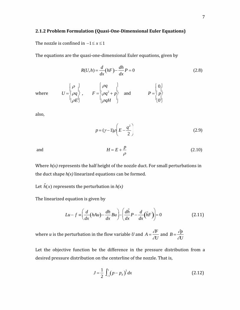
2.1.2 Problem Formulation (Quasi-One-Dimensional Euler Equations)

The nozzle is confined in

−1≤ x ≤1

The equations are the quasi-one-dimensional Euler equations, given by

R(U,h) =ddx

hF( )−dhdx

P = 0 (2.8)

where

U =ρρqρE

,

F =

ρqρq2 + pρqH

and

P =0p0

also,

p = (γ −1)ρ E −q2

2

(2.9)

and

H = E +pρ

(2.10)

Where h(x) represents the half height of the nozzle duct. For small perturbations in

the duct shape h(x) linearized equations can be formed.

Let

˜ h (x) represents the perturbation in h(x)

The linearized equation is given by

Lu − f ≡ddx

hAu( )−dhdx

Bu

−

d ˜ h dx

P −ddx

˜ h F( )

= 0 (2.11)

where u is the perturbation in the flow variable U and

A =∂F∂U

and

B =∂p∂U

Let the objective function be the difference in the pressure distribution from a

desired pressure distribution on the centerline of the nozzle. That is,

J =12

p − pd( )2 dx−1

1∫ (2.12)

8

The cost function sensitivity is given by

I =dJdh

˜ h = p − pd( ) dpdU

dUdh

˜ h −1

1∫ dx (2.13)

but

dUdh

˜ h = u

hence

I = p − pd( ) dpdU

u−1

1∫ dx (2.14)

Introduce the Lagrange multiplier v. A constraint on the objective function can be

enforced by letting,

J =12

p − pd( )2

−1

1∫ dx − vT Rdx−1

1∫ (2.15)

This ensures that the flow satisfies the equation of motion (2.8). That is,

R = 0 .

Then,

I =dJdh

˜ h = p − pd( ) dpdU

u−1

1∫ dx − vT (Lu − f )dx−1

1∫ (2.16)

Set,

dpdU

= gT , Then, consider

vT Ludx−1

1∫ =

vT ddx

hAu( )−dhdx

Bu

dx

−1

1∫

Integration by parts gives

vT Ludx−1

1∫ =

vT hAu( )−1

1−

dvT

dxhAu − vT dh

dxBu

dx

−1

1∫

9

Let

hAT dvdx

−dhdx

BTv = L*v (2.17)

Then

vT Ludx−1

1∫ =

vT hAu( )−1

1− L*v( )T

udx−1

1∫ (2.18)

Then

I = p − pd( )gT u−1

1∫ dx + vT fdx−1

1∫ − L*v( )Tudx

−1

1∫ − vT hAu( )−1

1 (2.19)

= vT fdx−1

1∫ − L*v − p − pd( )g( )Tudx

−1

1∫ − vT hAu( )−1

1

Now we can set

L*v − p − pd( )g = 0 (2.20)

This equation is the “Adjoint Equation” which can be solved for v.

This eliminates the dependence of cost function sensitivity on u except at the

boundaries. Inlet and exit conditions can be chosen to eliminate the explicit

dependence of I on u. That is,

vT hAu( )−1

1= 0 (2.21)

At a boundary where the flow equations have n incoming characteristics, and hence

n imposed boundary conditions, the adjoint equations will thus have (3-n) boundary

conditions corresponding to an equal number of incoming adjoint characteristics.

Then

I = vT fdx−1

1∫ (2.22)

Now, I tells us the rate of change or sensitivity of the objective function with respect

to change in the design parameter or parameters.

10

2.1.3 Example Problem

Assume that the duct shape is a function of a parameter

α

h(x) = α + 1−α( )x 2 (2.25)

Figure 2.1.1 shows the geometry of the duct with the throat area being equal to

α .

Note that,

∂h∂α

=1− x 2 (2.26)

Now return to the flow equation,

R(U,h(α)) = 0 (2.27)

Figure 2.1.1: A general parabolic shape of nozzle which depends on one design parameter.

11

The objective function is given by

J(U,α) . Linearization with respect to

α will give:

h = h +dhdα

dα and

F = F +dFdα

dα

Also,

Lu =ddx

hAu( )−∂h∂x

Bu (2.28)

and

f =∂ 2h

∂x∂αP −

ddx

dhdα

F

(2.29)

Hence

Lu = f can be solved for u.

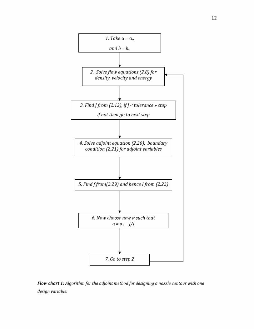
The design process is summarized in the flow chart 1. First take a guessed value of

design parameter α, say αo. The geometry for this value of design parameter is given

by equation (2.25). The governing equations (2.8) are then solved for the flow

properties ρ, p, E and u for the geometry corresponding to this value of design

parameter. The value of objective function corresponding to this geometry can now

be obtained using equation (2.12). The adjoint equations (given by (2.20)) are now

solved with boundary conditions (2.21) for the adjoint variables v1, v2 and v3. Now,

the values of the adjoint variables and flow properties are known inside the domain.

These values can be used to find the value of the sensitivity of the cost function with

respect to the design parameter. The sensitivity of the cost function with respect to

the design parameter is given by (2.22) and can directly be obtained using the

adjoint variables and f. The flow source term f can be obtained using the equation

(2.29). The new value of the design parameter(s) is found based on the steepest

descent method. The process is repeated until the objective function reaches the

desired minimum value.

12

Flow chart 1: Algorithm for the adjoint method for designing a nozzle contour with one

design variable.

1. Take α = αo

and h = ho

2. Solve flow equations (2.8) for density, velocity and energy

3. Find J from (2.12), if J < tolerance » stop

if not then go to next step

4. Solve adjoint equation (2.20), boundary condition (2.21) for adjoint variables

5. Find f from(2.29) and hence I from (2.22)

6. Now choose new α such that α = αo – J/I

7. Go to step 2

13

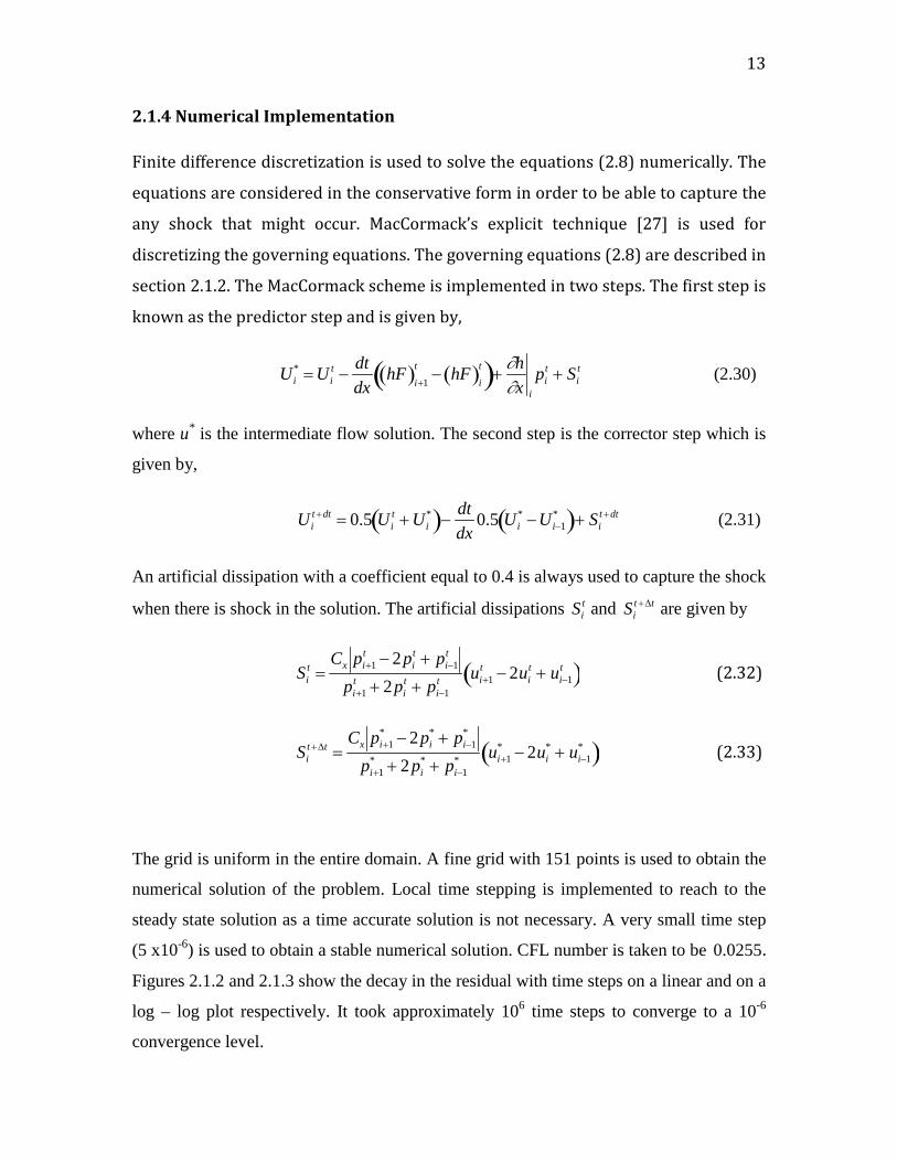
2.1.4 Numerical Implementation

Finite difference discretization is used to solve the equations (2.8) numerically. The

equations are considered in the conservative form in order to be able to capture the

any shock that might occur. MacCormack’s explicit technique [27] is used for

discretizing the governing equations. The governing equations (2.8) are described in

section 2.1.2. The MacCormack scheme is implemented in two steps. The first step is

known as the predictor step and is given by,

Ui* = Ui

t −dtdx

hF( )i+1

t − hF( )i

t( )+∂h∂x i

pit + Si

t (2.30)

where u* is the intermediate flow solution. The second step is the corrector step which is

given by,

Uit +dt = 0.5 Ui

t + Ui*( )−

dtdx

0.5 Ui* −Ui−1

*( )+ Sit +dt (2.31)

An artificial dissipation with a coefficient equal to 0.4 is always used to capture the shock

when there is shock in the solution. The artificial dissipations

Sit and

Sit +∆t are given by

Sit =

Cx pi+1t − 2pi

t + pi−1t

pi+1t + 2pi

t + pi−1t ui+1

t − 2uit + ui−1

t( ) (2.32)

Sit +∆t =

Cx pi+1* − 2pi

* + pi−1*

pi+1* + 2 pi

* + pi−1* ui+1

* − 2ui* + ui−1

*( ) (2.33)

The grid is uniform in the entire domain. A fine grid with 151 points is used to obtain the

numerical solution of the problem. Local time stepping is implemented to reach to the

steady state solution as a time accurate solution is not necessary. A very small time step

(5 x10-6) is used to obtain a stable numerical solution. CFL number is taken to be

0.0255.

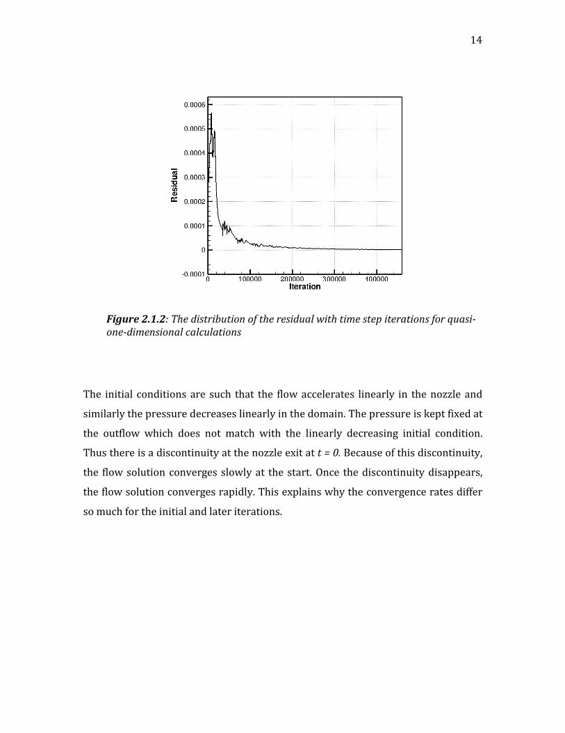
Figures 2.1.2 and 2.1.3 show the decay in the residual with time steps on a linear and on a

log – log plot respectively. It took approximately 106 time steps to converge to a 10-6

convergence level.

14

The initial conditions are such that the flow accelerates linearly in the nozzle and

similarly the pressure decreases linearly in the domain. The pressure is kept fixed at

the outflow which does not match with the linearly decreasing initial condition.

Thus there is a discontinuity at the nozzle exit at t = 0. Because of this discontinuity,

the flow solution converges slowly at the start. Once the discontinuity disappears,

the flow solution converges rapidly. This explains why the convergence rates differ

so much for the initial and later iterations.

Figure 2.1.2: The distribution of the residual with time step iterations for quasi-one-dimensional calculations

15

Figure 2.1.3: The distribution of the residual with time step iterations on a log – log plot for quasi-one-dimensional calculations.

16

2.2: Theory of Two Dimensional Adjoint Equations

2.2.1 Introduction

This section discusses the formulation of the two dimensional adjoint equations. A

Cartesian coordinate system is used to define the geometry. The physical space is

transformed to a uniform computational domain. The starting point is a system of

nonlinear partial differential equations describing a steady flow within some

computational domain. Curvilinear coordinates

(ξ,η) are used. Using these

coordinates, the partial differential equations describing the flow can be written as

R(U,α) = 0 (2.34)

where

U is the flow solution,

α are the design parameters and R is a nonlinear

differential operator which depends on the mapping from (x,y) to

(ξ,η) . Changing

the shape changes the mapping and hence R. Linearization of R will give the linear

partial differential equation

Lu = f (2.35)

where u is the perturbation in the flow field and f is the change due to the mapping.

Let J be the objective function and

α a vector of design variables. The aim is to find

the sensitivity of the objective function with respect to the design variables. If

J = J(U,α) then,

δJ =∂JT

∂αδα +

∂JT

∂UδU (2.36)

Similarly

δR =∂R∂α

δα +∂R∂U

δU = 0 (2.37)

Multiplying equation 2.37 by vT and subtracting from

δJ , given by 2.36, gives,

17

δJ =∂JT

∂αδα +

∂JT

∂UδU − vT ∂R

∂αδα +

∂R∂U

δU

(2.38)

Thus,

δJ =∂JT

∂α− vT ∂R

∂α

δα +

∂JT

∂U− vT ∂R

∂U

δU (2.39)

If v chosen to satisfy the adjoint equation,

∂JT

∂U− vT ∂R

∂U=0 (2.40)

then the sensitivity of the objective function will be independent of the flow solution

perturbation

δU . Solving the adjoint equation takes a computational effort equal to

that for one flow solution. This way it saves computational cost when multiple

design parameters are considered.

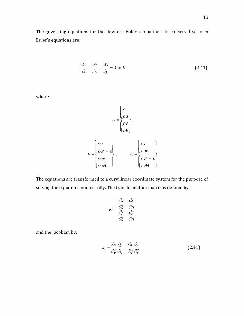
2.2.2 Problem Formulation

Consider the domain for the problem as the upper half of the nozzle. Only the upper

half is considered because the nozzle is assumed to be symmetric about the

centerline.

Figure 2.2.1: The general geometry of the nozzle for a two-dimensional case.

18

The governing equations for the flow are Euler’s equations. In conservative form

Euler’s equations are:

∂U∂t

+∂F∂x

+∂G∂y

= 0 in D (2.41)

where

U =

ρρuρvρE

,

F =

ρuρu2 + pρuvρuH

,

G =

ρvρuvρv 2 + pρvH

The equations are transformed to a curvilinear coordinate system for the purpose of

solving the equations numerically. The transformation matrix is defined by,

K =

∂x∂ξ

∂x∂η

∂y∂ξ

∂y∂η

and the Jacobian by,

Jc =∂x∂ξ

∂y∂η

−∂x∂η

∂y∂ξ

(2.41)

19

Introduce the contravariant velocity components

U 'V '

= K−1 uv

=1J

∂y∂η

−∂x∂η

−∂y∂ξ

∂x∂ξ

uv

(2.42)

Then , in the transformed plane

(ξ,η) , the equations are,

∂U '∂t

+∂F'∂ξ

+∂G '∂η

= 0 in D , (2.43)

where,

U '= J

ρρuρvρE

F '= J

ρU '

ρU 'u +∂ξ∂x

p

ρU 'v +∂ξ∂y

p

ρU 'H

,

G'= J

ρV '

ρV 'u +∂η∂x

p

ρV 'v +∂η∂y

p

ρV 'H

Now, the linearization of the fluxes with respect to the design parameter gives

If these relationships are introduced into the equations of motion (2.43), terms

independent of

˜ α will cancel each other and terms involving the square of

˜ α are

neglected as they are assumed to be small. The linearized equation can then be

written,

(2.44)

F → F +∂F∂U

∂U∂α

˜ α

G → G +∂G∂U

∂U∂α

˜ α

Lu = f

20

where,

and

A =∂F∂U

and

B =∂G∂U

The desired pressure distribution on the nozzle centerline is specified, and a nozzle

contour is to be found which gives this desired distribution. Let the cost function be

defined as the difference between the pressure at the centerline and the desired

pressure at the centerline. The goal is to minimize this cost function.

Thus the cost function is defined as,

J =12

p − pd( )2 dξ0

ξ m∫ (2.45)

Where pd is the desired pressure distribution at the nozzle centerline, p is the

calculated pressure distribution at the nozzle centerline, and

ξ m is the maximum

value of ξ, that is,

0 ≤ ξ ≤ ξ m

Now, multiply the governing equation by vT and subtract from the cost function. This

gives,

J =12

p − pd( )2 dξ0

ξ m∫ − vT Rdξ0

ξ m∫ (2.46)

The cost function sensitivity is given by,

I =∂J∂α

˜ α = p − pd( ) ∂p∂U

udξ0

ξ m∫ − vT Lu − f( )dξ0

ξ m∫ (2.47)

Lu =∂

∂ξAyη − Bxη( )u[ ]+

∂∂η

−Ayξ + Bxξ( )u[ ]

f =∂

∂ξF ∂

∂αyη − G ∂

∂αxη

u

+∂

∂η−F ∂

∂αyξ + G ∂

∂αxξ

u

21

where

u =∂U∂α

˜ α

That is,

I = p − pd( ) ∂p∂U

u − vT Lu

dξ

0

ξ m∫ + vT fdξ0

ξ m∫

Integration by parts and rearrangement leads to,

I = p − pd( ) ∂p∂U

u +∂vT

∂ξ(Ayη − Bxη )

dξ

0

ξ m∫ + vT fdξ0

ξ m∫ + vT (Ayη − Bxη )u0

ξ m

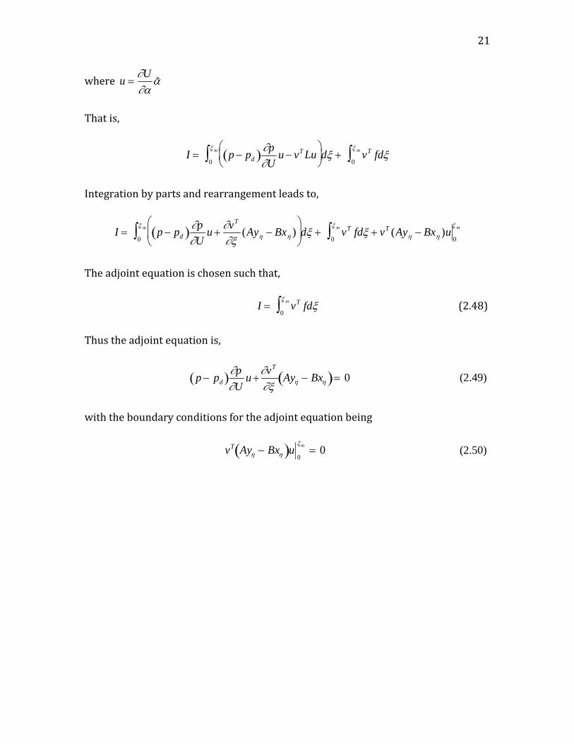
The adjoint equation is chosen such that,

I = vT fdξ0

ξ m∫ (2.48)

Thus the adjoint equation is,

p − pd( )∂p∂U

u +∂vT

∂ξAyη − Bxη( )= 0 (2.49)

with the boundary conditions for the adjoint equation being

vT Ayη − Bxη( )u0

ξm = 0 (2.50)

22

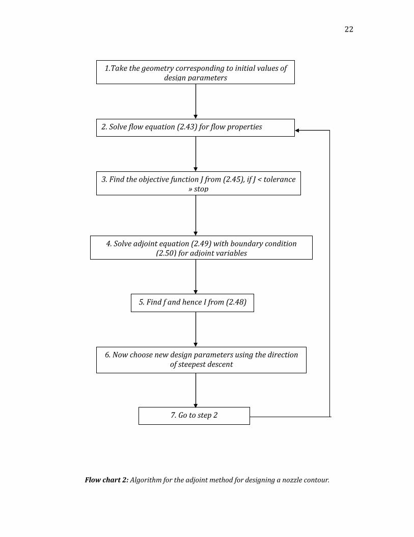
Flow chart 2: Algorithm for the adjoint method for designing a nozzle contour.

1.Take the geometry corresponding to initial values of design parameters

2. Solve flow equation (2.43) for flow properties

3. Find the objective function J from (2.45), if J < tolerance » stop

4. Solve adjoint equation (2.49) with boundary condition (2.50) for adjoint variables

5. Find f and hence I from (2.48)

6. Now choose new design parameters using the direction of steepest descent

7. Go to step 2

23

The process is summarized in flow chart 2. First, take a set of guessed values of the

design parameters α, say αo and find the geometry corresponding this set of design

parameters. The governing equations (2.43) are then solved for the geometry

corresponding to this set of design parameters for the flow properties ρ, p, v, E and

u. The value of the objective function corresponding to this geometry can now be

obtained using equation (2.45). The adjoint equations (2.49) are now solved with

the boundary conditions (2.50) to obtain the adjoint variables v1, v2, v3 and v4. The

value of the gradient of the cost function with respect to the design parameter then

can be directly obtained by equation (2.48) using the adjoint variables. A new value

of design parameter(s) is found based on the steepest descent method. The process

is repeated until the objective function reaches a desired minimum value.

24

2.2.3 Supersonic case with shocks:

In the case of supersonic flow a shock may occur in the flow domain inside the

nozzle. For example if the pressure ratio pa/po equals 0.67 a shock forms near the

nozzle exit. This discontinuity in the flow makes the objective function

discontinuous at the location of the shock, as the objective function is chosen to be

the integral of the pressure difference between the actual and desired values along

the nozzle centerline. With this discontinuity in the flow the adjoint equations can

not be solved. To remove the discontinuity in the objective function the objective

function is redefined as,

J =12

λ1Z2 + λ2

dZdξ

2

dξ

ξ 1

ξ m∫ − vT Rdξξ 1

ξ m∫ (2.51)

where Z is defined by equation (2.58). The gradient of the objective function with

respect to the design parameter(s) (also known as sensitivity) is given by,

I =dJdα

˜ α (2.52)

This leads to,

I = Z ∂p∂U

uξ 1

ξ m∫ dξ − vT (Lu − f )dξξ 1

ξ m∫ where

u =∂U∂α

˜ α

Hence, in this formulation Z replaces (p-pd). Here

ξ1 ≤ ξ ≤ ξm is the centerline coordinate. In this particular case

ξ1 = 0

Integration by parts and rearrangement leads to,

I = Z ∂p∂U

u − vT Lu

dξ +

0

ξ m∫ vT fdξ0

ξ m∫ (2.53)

The adjoint equation is chosen such that,

25

I = vT fdξ0

ξ m∫ (2.54)

Thus the adjoint equation is,

Z ∂p∂U

u +∂vT

∂ξAyη − Bxη( )= 0 (2.55)

with the boundary conditions for the adjoint equation being chosen such that,

vT Ayη − Bxη( )u0

ξm = 0 (2.56)

During the derivation of the adjoint equation it is also necessary to enforce the condition,

Z dδZdξ

ξ1

ξ m

= 0 . (2.57)

From this it is chosen that Z(

ξ 1)=Z(

ξ m)=0.

Z is calculated numerically in the domain.

The values of

λ1 and

λ2 are chosen such that the equation,

λ1Z − λ2d2Zdξ 2 = p − pd (2.58)

has a smooth solution for Z.

The solution procedure is,

1. solve the flow equation

2. solve for the shock parameter Z

3. solve the adjoint equation

4. calculate the value of the objective function

5. correct the design parameter in the direction of steepest descent

26

2.2.4 Numerical Implementation

The two-dimensional physical space is mapped to a uniform computational space.

Cartesian coordinates (x,y) are transformed to a uniform computational

domain

(ξ,η) . Every constant

ξ line corresponds to a constant x line and every

constant

η line corresponds to a contour in the y direction. The grid distribution is

uniform in the

η direction but it is not uniform in

ξ direction. Figure 2.2.2 shows

the grid inside the domain. The distribution of the increment dx is shown in figure

2.2.3. This distribution is chosen such that the flow in the convergent and divergent

sections is captured accurately. There is more clustering near the outflow and less

clustering near the inflow. A fine grid with 201x21 points is used to obtain the

numerical solution of the problem. A very small time step (5 x10-7) is used to get a

stable numerical solution. The CFL number is taken to be

0.0068.

Figure 2.2.2: Mesh inside the nozzle domain for two-dimensional calculations.

27

Local time stepping is used to obtain the steady solution. The second order explicit finite

difference MacCormack scheme is used to find the flow solution [27]. It is a predictor

corrector scheme. The first step is known as predictor step given by,

ui, j* = ui, j

t −dtdξ

f i+1, jt − f i, j

t( )−dtdη

gi, j +1t − gi, j

t( )+ Si, jt (2.59)

where u* is the intermediate flow solution. The second step is the corrector step, which is

given by,

ui, jt +∆t = 0.5 ui, j

t + ui, j*( )−

dtdξ

0.5 f i, j* − fi−1, j

*( )−dtdη

0.5 gi, j* − gi, j−1

*( )+ Si, jt +∆t (2.60)

Where

ui, jt ,gi, j

t and

fi, jt are the components of the vectors defined by equation (2.43) at

the grid point i, j and time step t.

Figure 2.2.3: The distribution of increment dx with grid points along the nozzle centerline.

28

Artificial dissipation with a coefficient 0.4 is used to smooth the shock when there is

shock in the solution. The artificial dissipation factors are

Si, jt and

Si, jt +∆t , given by

Si, jt =

Cx pi+1, jt − 2pi, j

t + pi−1, jt

pi+1, jt + 2pi, j

t + pi−1, jt ui+1, j

t − 2ui, jt + ui−1, j

t( )+Cy pi, j +1

t − 2 pi, jt + pi, j−1

t

pi, j +1t + 2 pi, j

t + pi, j−1t ui, j +1

t − 2ui, jt + ui, j−1

t( ) (2.61)

Si, jt +∆t =

Cx pi+1, j* − 2pi, j

* + pi−1, j*

pi+1, j* + 2pi, j

* + pi−1, j* ui+1, j

* − 2ui, j* + ui−1, j

*( )+Cy pi, j +1

* − 2pi, j* + pi, j−1

*

pi, j +1* + 2pi, j

* + pi, j−1* ui, j +1

* − 2ui, j* + ui, j−1

*( ) (2.62)

Figures 2.2.4 and 2.2.5 show the decay in the residual with time steps on a direct and on a

log – log plot respectively. The behavior of the residual can be explained by the initial

conditions. Initial conditions are such that the pressure decreases linearly in the

nozzle and reaches its minima at the nozzle exit. The boundary conditions are such

that pressure is kept fixed at the nozzle exit which is much higher than the linearly

described pressure value, hence there develops a discontinuity at the nozzle exit.

Because of this discontinuity the convergence rate is smaller to start with. Once the

discontinuity disappears, the flow solution converges much more rapidly.

29

Figure 2.2.4: The decay of the residual with time iterations.

Figure 2.2.5: The decay of residual with time iterations on a log – log plot.

30

In this chapter the formulation of the adjoint equations has been discussed for

quasi-one-dimensional and two-dimensional Euler equations. The use of the adjoint

equation to find the gradient of the cost function with respect to the design

parameters is then explained. The geometry that gives an optimum value of cost

function can be found using these gradients. The case when there is shock inside the

nozzle is considered separately and the formulation is described for that case. The

chapter then briefly describes the numerical implementation of these methods. In

the next chapter the results of the use of these methods are given. The geometry

that gives an optimum value of the cost function is obtained for quasi-one-

dimensional and two-dimensional cases. These results are discussed in the next

chapter.

31

Chapter 3: Results and Discussion

In the previous chapter it was shown how adjoint methods could be used to

determine a nozzle shape with particular flow characteristics. To assess the method

further, a desired pressure distribution is taken to be such that the corresponding

nozzle shape is known. For this known shape, the pressure distribution at the nozzle

centerline is calculated by solving the Euler equations (one or two dimensional).

Then the shape is perturbed from the desired one. The first design cycle uses this

new shape to find the flow solution. Then the adjoint solution and hence the

gradient of the objective function with respect to the design parameter(s) is

determined. This gradient is used to calculate the next value of design parameter as

follows

α new = α old −J

∂J∂α( )

. (3.1)

Here

α new is the new value of the design parameter,

α old is the previous value of the

design parameter,

J is the objective function corresponding to the previous value of

the design parameter, and

∂J∂α

is the gradient of the objective function with respect

to the previous value of the design parameter (calculated using adjoint methods).

When there are several design parameters {

α i}

α inew = α i

old −J

∂J∂α i

(3.2)

Either (3.1) or (3.2) is iterated until the value of the objective function reaches a

desired limit: usually a small value. It generally takes small number of iterations to

reach to the desired limit. This is discussed in detail along with a discussion of the

individual cases.

32

Quasi-one-dimensional and two-dimensional cases are considered to determine the

nozzle shape that gives the desired pressure distribution on the nozzle centerline.

Both subsonic and supersonic flows are considered. The findings are compared with

earlier results by Giles [7] and Jameson [1]. The general properties of the one-

dimensional results match those that Giles had anticipated. Two different kinds of

nozzle geometries are considered for the two-dimensional case – one with one

design parameter and other with three design parameters.

3.1 Quasi-one-dimensional Nozzle

A convergent-divergent nozzle is considered here. The use of the adjoint method to

determine a geometry which gives the desired pressure distribution is

demonstrated. The nozzle under consideration has a very simple shape given by a

parabola. That is,

h(x) = α + 1−α( )x 2 (3.3)

Figure 3.1.1: Initial and final nozzle shapes. The black line shows the final geometry and the red line shows the initial shape for quasi-one-dimensional flow.

33

The parabola depends on a single parameter α. As discussed earlier, the flow inside

a nozzle depends mainly on the axial position and area ratio. Hence, the quasi-one-

dimensional equations (2.8) are considered to determine the flow properties inside

the nozzle.

Figure 3.1.1 shows the geometry of the nozzle. Note that the actual equations are

quasi-one-dimensional. The exact shape changes with the value of the design

parameter α. The desired pressure distribution corresponds to value of α = 0.8. This

geometry is shown in black in the figure. This is the value which is needed to be

reached by the adjoint design method. To start the design procedure, the initial

value of α is taken to be 0.68, the corresponding geometry is shown by the red line

in figure 3.1.1. The corresponding pressure distribution is found numerically at the

nozzle centerline for a subsonic case. The geometry is parabolic and the area ratio

(Ae/Ao) is equal to one and so is the pressure ratio. To ensure that there is a flow

inside the nozzle, a small velocity has been assigned at the inflow. The flow

accelerates inside the nozzle and then it decelerates to have the exit Mach number

equal to the inlet Mach number. After the first design cycle, the value of α obtained

is 0.6779. This value of α is now used to obtain the next value of α. The MacCormack

scheme [27] is used to determine the flow solution. Details of the numerical method

are given in section 2.1.4.

Figure 3.1.2: The convergence of the objective function with design cycles for quasi-one-dimensional flow.

34

Figure 3.1.4: The convergence of the design parameter α with design cycles for quasi-one-dimensional flow.

Figure 3.1.3: The convergence of objective function with design cycles on a log-log plot for quasi-one-dimensional flow.

35

The decrease in the value of (p-pd)2 (i. e. the difference in the desired and numerical

pressure) is rapid initially and gradual afterwards, hence the objective function

drops rapidly for first few design cycles and then it drops more gradually as shown

in figure 3.1.2. The objective function shows a very good rate of convergence as does

the design parameter as shown in figure 3.1.4. It took approximately 17 design

cycles to converge to a value of α = 0.80009. The corresponding value of objective

function is 73.93 (N/m2)2, which is a drop from its initial value of 8.563 x 104

(N/m2)2. Figure 3.1.5 shows the convergence of the design parameter α with design

cycles on a log – log plot. The design parameter converges steadily towards the

desired value.

Figure 3.1.5: The convergence of the difference of design parameter α and required design parameter αο with design cycles on a log-log plot for the quasi-one-dimensional flow.

36

Figure 3.1.6 shows the initial, final and desired pressure distributions. The initial

pressure distribution is given by red in the figure. The final pressure distribution is

given by blue which overlaps the desired pressure distribution (symbols). The

maximum difference between initial and final pressure distributions is

approximately 20000 N/m2. Τhe difference between the desired and final pressure

distributions is negligible. Hence, from now onwards, there is no need for additional

design cycles and it can be observed from the α and objective function convergence

plots, figures 3.1.4 and 3.1.2, that the change is negligible after a certain number of

design cycles.

Figure 3.1.6: The distribution of the final, desired and initial pressure distribution (with respect to total pressure po) as function of axial distance inside nozzle. The symbols represent the desired pressure distribution, the blue line represents the final pressure distribution, and the red line represents the initial pressure distribution for quasi-one-dimensional flow.

37

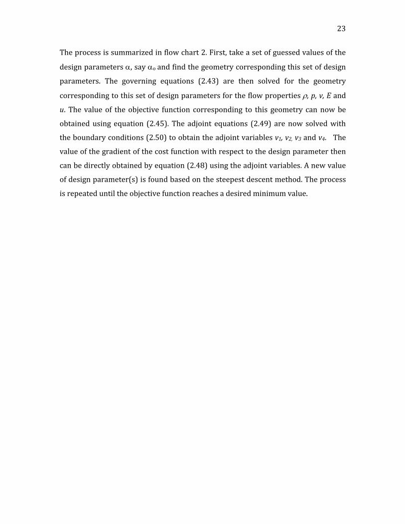
Figure 3.1.7: The distribution of the adjoint variable v1 with axial distance inside the nozzle for quasi-one-dimensional flow.

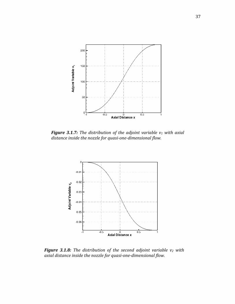
Figure 3.1.8: The distribution of the second adjoint variable v2 with axial distance inside the nozzle for quasi-one-dimensional flow.

38

Figures 3.1.7 – 3.1.9 show the distribution of the adjoint variables v1, v2 and v3 along

the nozzle centerline for the final geometry. As discussed in previous work by Giles

(8), adjoint variables are continuous inside the domain. However, one thing to take

note of is that these variables are not equal to zero at the nozzle exit. This seemed to

be a requirement in the formulation of the method in order to eliminate the

dependence on the flow variable fluctuations but the actual requirement is that the

derivative

∂v∂x should be zero at the inlet and the outlet. At the inlet a Dirichlet

boundary condition is implemented so that the adjoint variables are zero. The outlet

boundary is kept free which shows that although the adjoint variables are not zero,

their gradients are, which is the requirement of the method. It should be recalled

that the inner product of the adjoint variables with the right hand side of the

linearized flow equations, which depends on the geometry, gives the sensitivity of

the cost function to the design parameter(s).

Figure 3.1.9: The distribution of the initial adjoint variable v3 with axial distance the nozzle for quasi-one-dimensional flow.

39

3.2 Two-dimensional Nozzle

A two-dimensional nozzle is considered for this case. The flow is considered to be

inviscid and the two-dimensional compressible inviscid equations are used as the

governing equations in conservative form (section 2.2.2). Two different cases are

considered in this section. First, a simple case where the nozzle geometry depends

on only one design parameter is studied. A subsonic flow solution is found for this

case. The second case is where the nozzle geometry depends on three design

parameters. All three design parameters are varied and design iterations are

performed to obtain the desired centerline pressure distribution. First the subsonic

case is presented and then a case where a shock forms inside the nozzle is

presented.

3.2.1 One Design Parameter

To demonstrate the design method a simple case is considered first. A nozzle shape

is introduced that is governed by only one design parameter. This parameter is

denoted by

α . The nozzle contour is given by the equations,

y =1.75 − (0.5 + α)cos((0.2x −1)π ) for

0 ≤ x ≤ 5

y =1.25 −α cos((0.2x −1)π ) for

5 ≤ x ≤10 (3.4)

Figure 3.2.1: The initial (red), intermediate (green) and final (black) geometry of the rectangular nozzle.

40

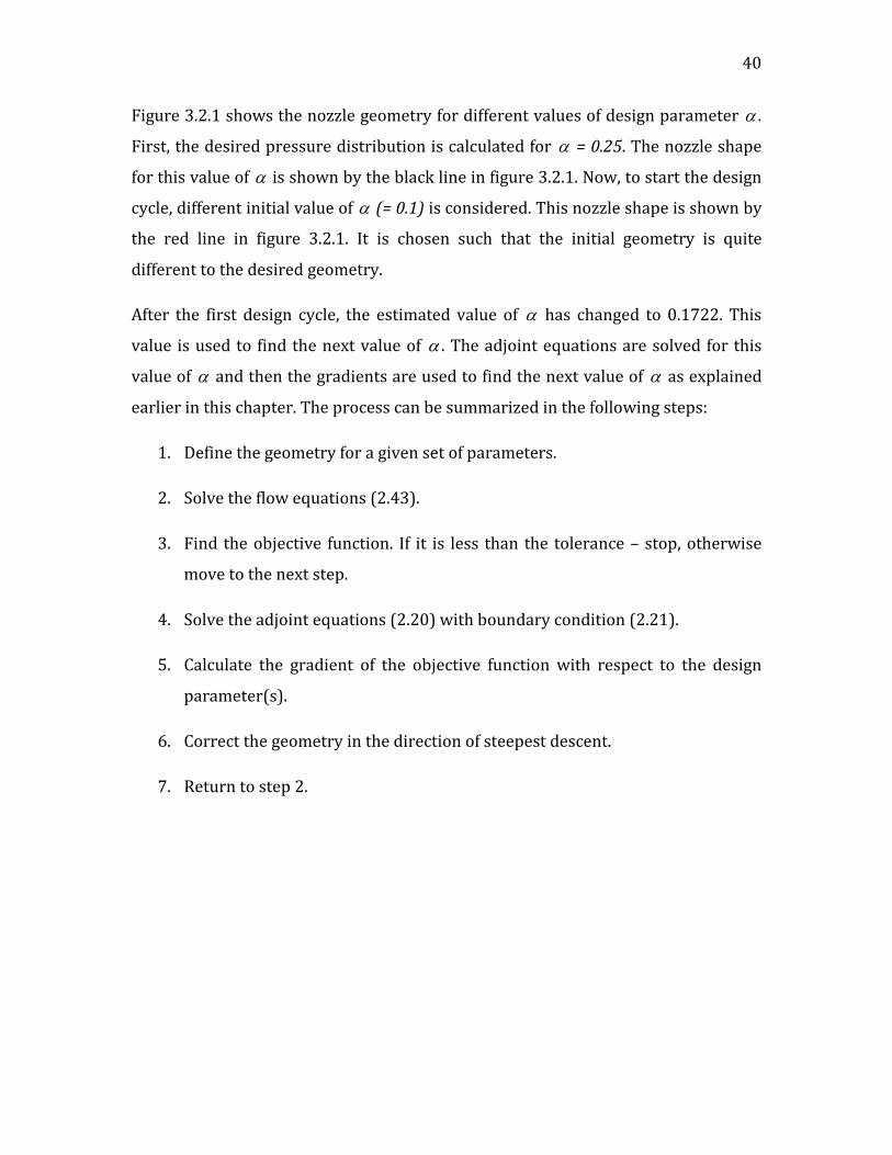
Figure 3.2.1 shows the nozzle geometry for different values of design parameter

α .

First, the desired pressure distribution is calculated for

α = 0.25. The nozzle shape

for this value of

α is shown by the black line in figure 3.2.1. Now, to start the design

cycle, different initial value of

α (= 0.1) is considered. This nozzle shape is shown by

the red line in figure 3.2.1. It is chosen such that the initial geometry is quite

different to the desired geometry.

After the first design cycle, the estimated value of

α has changed to 0.1722. This

value is used to find the next value of

α . The adjoint equations are solved for this

value of

α and then the gradients are used to find the next value of

α as explained

earlier in this chapter. The process can be summarized in the following steps:

1. Define the geometry for a given set of parameters.

2. Solve the flow equations (2.43).

3. Find the objective function. If it is less than the tolerance – stop, otherwise

move to the next step.

4. Solve the adjoint equations (2.20) with boundary condition (2.21).

5. Calculate the gradient of the objective function with respect to the design

parameter(s).

6. Correct the geometry in the direction of steepest descent.

7. Return to step 2.

41

Figure 3.2.2: The pressure distribution (with respect to total pressure po) along

the centerline of the nozzle. The red and blue lines show the initial and final

pressure respectively along the nozzle centerline. The desired pressure is shown

Figure 3.2.3: The Mach number distribution along the centerline of the nozzle. The red

and blue lines show the initial and final Mach number respectively along the nozzle

centerline. The desired Mach number is shown by symbols.

42

Figure 3.2.4: The decay of the objective function with design cycles. It decays rapidly initially and then it converges steadily to zero. The second plot shows the same data on a log-log scale.

43

Figure 3.2.6: The convergence of the design parameter with respect to the desired value of design parameter (α−αο ) with design cycles on a log – log plot .

Figure 3.2.5: Change in the design parameter α with design cycles. The desired value of design parameter is 0.25.

44

This procedure gives the value of

α to be 0.2497 in 10 design cycles. For this value

of design parameter the flow properties in the nozzle match closely with the desired

values (figures 3.2.2 and 3.2.3). The decay of the objective function with design

cycles is shown in figure 3.2.4, it decays rapidly initially and then it decays steadily

to close to zero. To understand the convergence of the objective function, it is shown

on a log-log plot in figure 3.2.4. The convergence of

α on the log-log plot is shown in

figure 3.2.6. These convergence rates are lower that the convergence rates of the

one-dimensional solution. It was observed that after 10 design cycles

α keeps on

fluctuating and does not converge any further. It reaches the proximity of the

desired value and then it keeps oscillating around that. The reason for the

oscillations can be given by the fact that pressure distribution is already close to the

desired pressure distribution and further design cycles are not really useful. It could

also be the limit of the resolution of the numerical solution.

45

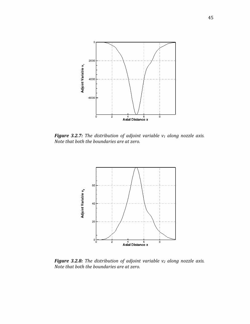
Figure 3.2.8: The distribution of adjoint variable v2 along nozzle axis. Note that both the boundaries are at zero.

Figure 3.2.7: The distribution of adjoint variable v1 along nozzle axis. Note that both the boundaries are at zero.

46

Figure 3.2.9: The distribution of adjoint variable v3 along nozzle axis. Note that both the boundaries are at zero.

Figure 3.2.10: The distribution of adjoint variable v4 along nozzle axis. Note that both the boundaries are at zero.

47

The distribution of the adjoint variables for final design cycle is shown in the figures

3.2.7 - 3.2.10 for a subsonic flow. The adjoint variables are continuous throughout

the nozzle for the subsonic case. In the two dimensional case, adjoint variables have

values of zero at both boundaries. Zero Dirichlet boundary conditions have to be

implemented numerically in order to obtain the solution of the adjoint equations.

This is different than the one-dimensional case. For the one-dimensional case the

values of the adjoint variables are non-zero at the outflow boundary. For the one-

dimensional case no boundary condition was needed at the outflow boundary. The

value of the third adjoint variable is zero throughout on the centerline (figure 3.2.9).

The third adjoint variable corresponds to the y component of the velocity and that is

zero on the centerline of the nozzle. This indicates that the gradient of the objective

function is independent of the y component of velocity on centerline, which is, of

course, zero. Figures 3.2.2 and 3.2.3 show the distribution of Mach number and

pressure respectively at the nozzle centerline. The value of pe/po is kept constant

and is equal to 0.93 to ensure subsonic flow inside the nozzle. The initial and final

flow properties are quite different from each other. The final flow properties are

equal to the desired flow properties which shows that very good convergence is

achieved through this method. The flow solutions for the initial and final geometries

inside the whole nozzle domain are shown for a case of subsonic flow in figure

3.2.11. It can be noticed that the initial and final flows are quite different especially

at the nozzle throat. A low-pressure zone extends for the final flow at the throat

which is same as the desired condition.

48

3.2.2 Three design parameters

In this section a more complicated nozzle geometry is considered to show the

advantage of the adjoint method. In this case the nozzle geometry depends on three

design parameters. This is the practical case as adjoint methods are most cost

effective when there are several design parameters. The design parameters are

denoted by

α1,

α2 and

α3 . The nozzle contour equations are ,

Figure 3.2.11: Pressure contours inside the nozzle. The upper half of the nozzle shows the

pressure contours for the initial geometry and the lower half shows the pressure contours

for the final geometry.

49

for

0 ≤ x ≤ 5

y =1.75 − (0.5 + α1)cos((0.2x −1)π ) −α2 cos((0.2x −1)π ) + α3 cos((0.2x −1)π )

for

5 ≤ x ≤10

y =1.25 −α1 cos((0.2x −1)π ) −α2 cos((0.2x −1)π ) + α3 cos((0.2x −1)π ) (3.5)

The equation (3.5) is such that α2 and α3 can be combined to give one new design

parameter. Then the geometry will depend only on two design parameters. Breaking

up the geometry into more parts gives the freedom of perturbing the geometry in

more places.

Figure 3.2.12: The geometry of the nozzle. Calculations were performed for only half the

domain. The red line shows the initial geometry. The green line shows the final geometry. The

black line shows the geometry that gives the desired pressure distribution.

50

The use of the adjoint design methods is demonstrated here to calculate more than

one gradient of the objective function. The nozzle geometry depends on three design

parameters and hence the gradients of the objective function for these three design

parameters are calculated using adjoint methods. The desired shape is such that it

gives a desired pressure distribution on the nozzle centerline. The initial area ratio

(Ae/Ao) is equal to 0.6 and the pressure ratio (pe/po) corresponding to ideal subsonic

flow will be 0.92. A subsonic case with pe/po = 0.93 has been considered here.

The desired geometry corresponds to values of

α1,

α2 and

α3 of 0.25, 0.25 and 0.25

respectively. The initial geometry is taken to be such that the values are 0.1, 0.1 and

0.1 respectively. This gives exactly the same geometry as was considered for the one

parameter case. These geometries are shown in figure 3.2.12. The red line shows the

initial geometry. The black line shows the desired geometry and the green line

shows the final geometry given by the adjoint design. After the first design cycle the

values of

α1,

α2 and

α3 are found to be 0.1721, 0.1721 and 0.0280 respectively.

These values are used to find the next values of

α i. The adjoint equations are solved

for the geometry given by these values and then the gradients are used to find the

next value of

α i, as explained earlier. The process can be summarized in the

following steps:

1. Define the geometry for a given set of parameters.

2. Solve the flow equations (2.43).

3. Find objective function, if it is less than the tolerance – stop, otherwise move

to the next step.

4. Solve the adjoint equations (2.49) with boundary conditions (2.50).

5. Calculate the gradients of the objective function with respect to the design

parameter(s).

6. Correct the mapping in the direction of steepest descent.

51

7. Return to step 2.

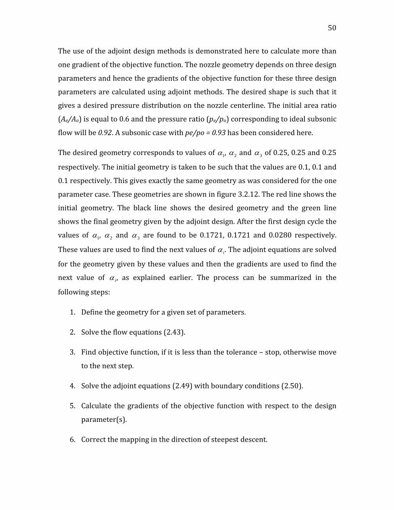
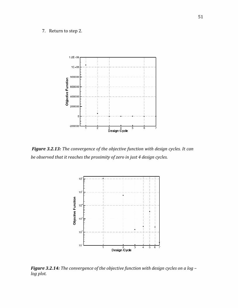
Figure 3.2.14: The convergence of the objective function with design cycles on a log – log plot.

Figure 3.2.13: The convergence of the objective function with design cycles. It can

be observed that it reaches the proximity of zero in just 4 design cycles.

52

In this case it took approximately 7 design cycles to converge to the desired shape. It

can be observed that the final and desired geometry match quite well (figure

3.2.12). The value of the objective function after 7 design cycles is equal to 36.38

(N/m2)2 which is a decrease from an initial value 1.042 x 106 (N/m2)2. So it has

dropped by a more than four orders of magnitude. The convergence of the objective

function is shown in figure 3.2.13. It shows a very good convergence rate which can

be seen on a log – log plot (figure 3.2.14). It is observed that the objective function

drops rapidly initially and then it gradually approaches zero. The rate of

convergence is higher than the one in the case of one parameter only. From the log –

log plot it can be seen that the objective function keeps on oscillating about a small

minimum value. This may be due to the resolution limit of the grid in the flow

simulation.

Figure 3.2.15: The convergence of design parameter α1 with design cycles.

53

Figure 3.2.16: The convergence of design parameter α2 with design cycles.

Figure 3.2.17: The convergence of design parameter α3 with design cycles.

54

The convergence of

α i is shown in figures 3.2.15-3.2.17. One interesting thing about

the results is that although the final geometry matches quite well with the desired

geometry (as do the flow properties), the design parameters do not individually

meet the desired design parameters. The set of design parameters for which the

desired pressure distribution was found is (0.25, 0.25, 0.25) whereas the final set

converged values of design parameters is (0.1502, 0.1502, 0.049794). The geometry

contour given by (3.5) is same for these two sets of design parameters which means

that although the design parameters do not reach the desired set of values, the

geometry does. These values effectively reach their final value in just three design

cycles but they keep on oscillating around those values with more design cycles. The

method could have been truncated at three design cycles where the objective

function has a value equal to 154.2 (N/m2)2.

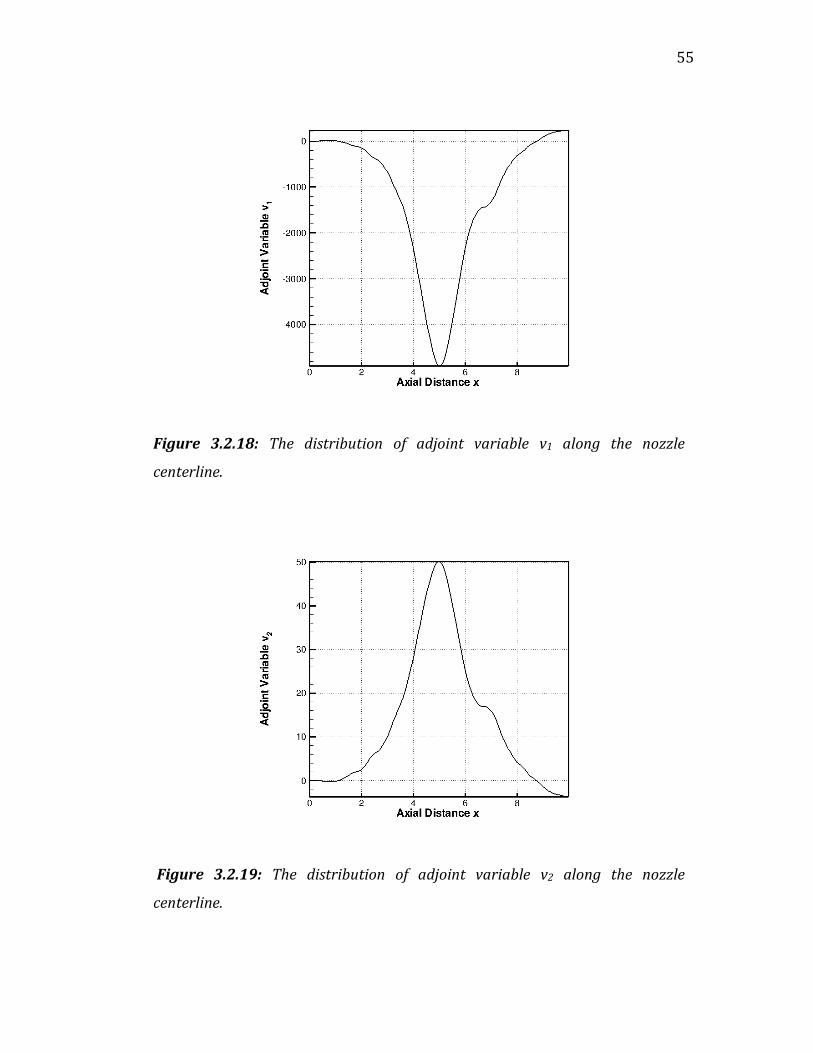
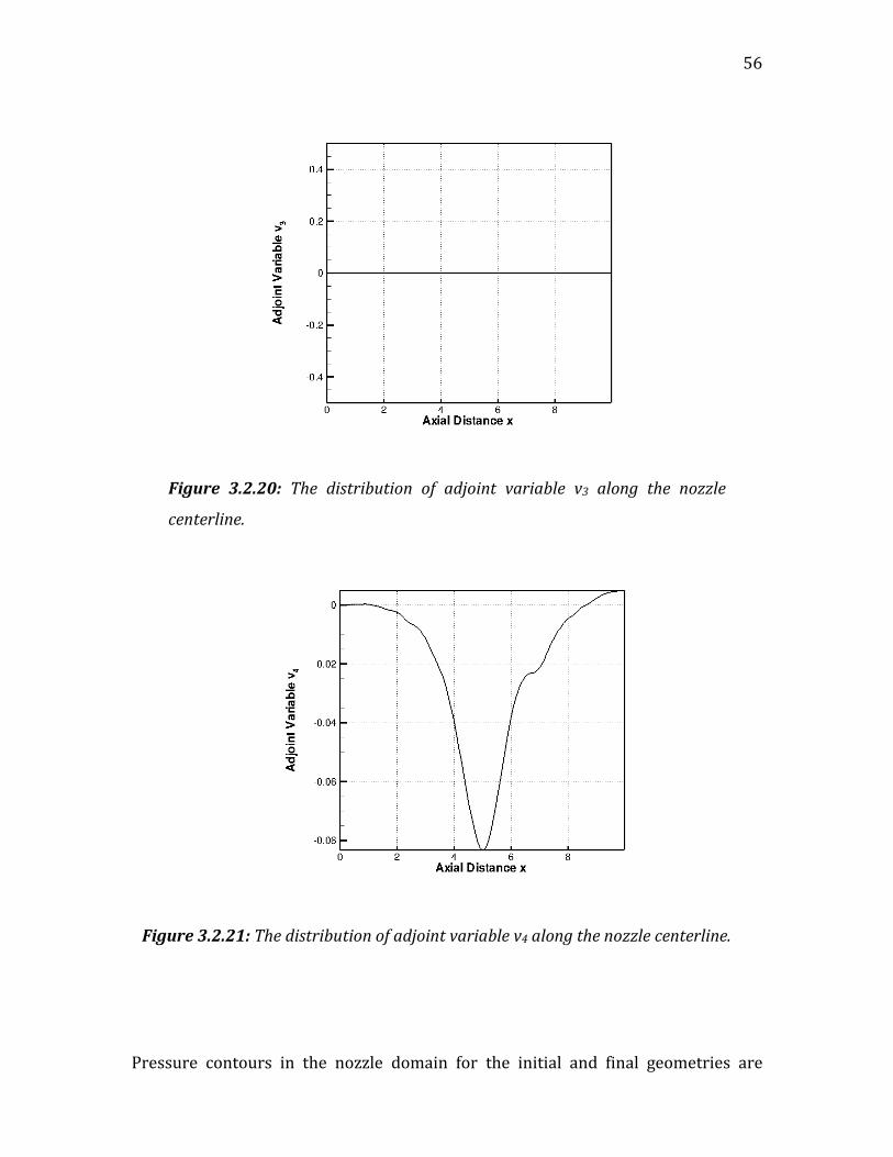
Figures 3.2.18 – 3.2.21 show the distributions of the adjoint variables along the

nozzle centerline for the final design cycle. For the subsonic case, the adjoint

variables are continuous on the centerline. The third adjoint variable (figure 3.2.20)

is zero everywhere on the centerline. It corresponds to the y component of the

velocity. This indicates that the gradient of the objective function is independent of

the y component of velocity on the centerline, which is, of course, zero. Adjoint

variables depend on the flow solution and geometry. As the desired geometry is

same for one parameter and three parameter cases, the distribution of adjoint

variables is very similar for both the cases. Note that the pressure ratio pe/po is kept

same for both cases (= 0.93 for subsonic flow).

55

Figure 3.2.18: The distribution of adjoint variable v1 along the nozzle

centerline.

Figure 3.2.19: The distribution of adjoint variable v2 along the nozzle

centerline.

56

Pressure contours in the nozzle domain for the initial and final geometries are

Figure 3.2.21: The distribution of adjoint variable v4 along the nozzle centerline.

Figure 3.2.20: The distribution of adjoint variable v3 along the nozzle

centerline.

57

shown in figure 3.2.22. It can be seen that the initial and final flows are quite

different. The red and blue lines in the figure 3.2.22 respectively show the initial and

final pressure distribution on the nozzle centerline. The desired pressure

distribution on the nozzle centerline is shown by symbols. The flow properties on

the nozzle centerline match very well with the desired flow property distribution.

The pressure contours inside the entire nozzle domain are shown in figure 3.2.23. It

can be observed from that figure that the initial and final flows are very different

although the exit pressure ratio is kept constant for a subsonic flow inside the

nozzle.

Figure 3.2.22: The pressure distribution (with respect to total pressure po)

along the centerline of the nozzle. The red and blue lines show the initial and

final pressure respectively along the nozzle centerline. The desired pressure is

shown by black symbols.

58

Figure 3.2.23: The pressure contours inside the nozzle. The upper half of the nozzle shows the

pressure contours for the initial geometry and lower half shows the pressure contours for the

final geometry.

59

3.2.3 Supersonic case with shocks

In this section a case is presented where there is shock in the flow solution. In such a

case, the flow in not continuous in the nozzle. Hence, calculations can not be

performed in the same way as for a shock free case. As already discussed previously

a new parameter Z is introduced such that new cost function in terms of Z is

continuous across the shock (see equation (2.58)). A nozzle contour is considered

which depends on three parameters. The design parameters are denoted by

α1,

α2

and

α3 . The nozzle contour equations are,

for

0 ≤ x ≤ 5

y =1.75 − (0.5 + α1)cos((0.2x −1)π ) −α2 cos((0.2x −1)π ) + α3 cos((0.2x −1)π )

for

5 ≤ x ≤10

y =1.25 −α1 cos((0.2x −1)π ) −α2 cos((0.2x −1)π ) + α3 cos((0.2x −1)π ) (3.6)

The initial geometry is taken such that the values of design parameters

α1,

α2 and

α3 are 0.1, 0.1 and 0.1 respectively. The desired geometry is such that the values of

the design parameters

α1,

α2 and

α3 are 0.25, 0.25 and 0.25 respectively. The initial

area ratio (Ae/Ao) is equal to 0.6 and the pressure ratio corresponding to ideal

supersonic flow will be 0.17. The value of pressure ratio (pe/po) is taken to be 0.67 to

ensure shocks in the nozzle. After the first design cycle the values of

α1,

α2 and

α3

are found to be 0.1101, 0.11001 and 0.0899 respectively. The flow equation is solved

for the new geometry defined by these values. Then the value of shock parameter is

calculated to smooth the cost function. This is an extra step for the discontinuous

flows. The adjoint equations are solved again and the gradients are used to find the

next values of the design parameters. The process can be summarized as follows:

60

1. Define the geometry for an initial set of parameters.

2. Solve the flow equation (2.43).

3. Find objective function, if it is less than the tolerance – stop, otherwise move

to the next step.

4. Smooth the cost function if necessary (supersonic case with shocks).

5. Solve the adjoint equations.

6. Calculate the gradient of the objective function with respect to the design

parameter(s).

7. Correct the mapping in the direction of steepest descent.

8. Return to step 2.

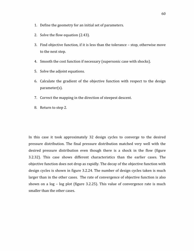
In this case it took approximately 32 design cycles to converge to the desired

pressure distribution. The final pressure distribution matched very well with the

desired pressure distribution even though there is a shock in the flow (figure

3.2.32). This case shows different characteristics than the earlier cases. The

objective function does not drop as rapidly. The decay of the objective function with

design cycles is shown in figure 3.2.24. The number of design cycles taken is much

larger than in the other cases. The rate of convergence of objective function is also

shown on a log – log plot (figure 3.2.25). This value of convergence rate is much

smaller than the other cases.

61

Figure 3.2.24: The decay of objective function with design cycles for the supersonic case with a shock.

Figure 3.2.25: The convergence of objective with design cycles on a log – log plot for the supersonic case with a shock.

62

The convergence of

α i is shown in figures 3.2.26-3.2.28. They gradually converge to

the values that are not the originally desired values, but the geometry given by the

converged values is very similar to the desired geometry. The set of design

parameters for which the desired pressure distribution was found is (0.25, 0.25,

0.25) whereas the final set of the converged values of design parameters is (0.1502,

0.1502, 0.04979). Unlike other cases these value take several design cycles to

converge. It took approximately 32 design cycles to reach the proximity of the

desired pressure distribution. It is probable that this reflects the limit of the grid to

resolve smaller changes in the pressure distribution.

Figure 3.2.26: The convergence of the design parameter α1 with design cycles.

63

Figure

Figure 3.2.27: The convergence of the design parameter α2 with design cycles.

Figure 3.2.28: The convergence of the design parameter α3 with design cycles.

64

3.2.29 shows the distribution of pressure on the nozzle centerline. The initial

pressure distribution is shown by a red line. The final pressure distribution is

shown by blue line. The desired pressure distribution is shown by symbols in figure

3.2.29. All these calculations are performed for a fixed value of pressure ratio pe/po

(= 0.67). Initially, the shock was at the nozzle exit and it keeps on moving inside the

nozzle with each design cycle. The final and desired pressure distributions do not

agree exactly but they are very close. The presence of the shock increases the value

of objective function. The initial value of the objective function is 4.39 x 106 (N/m2)2

which drops to a value of 2.13 x 105 (N/m2)2 after 32 design cycles which is a

decrease of 95.14%. The full flow solution for the initial (upper) and final (lower)

geometries inside the nozzle domain is shown in figure 3.2.30. Pressure contours

are shown in the domain. The difference in the two solutions is basically the shock

location. The nozzle is sonic at the throat hence the flow upstream of the throat

remains the same. Whereas, the flow downstream changes with each design cycle.

Figure 3.2.29: The distribution of pressure (with respect to total pressure po)

along nozzle centerline. The red and blue lines show the initial and final

pressure respectively along the nozzle centerline. The desired pressure is shown

by black symbols.

65

Figure 3.2.30: Pressure contours inside the nozzle domain. Upper half shows the initial flow and lower half shows the final flow.

Figure 3.2.31: The distribution of shock parameter Z along nozzle axis for the final design cycle.

66

Figure 3.2.31 shows the distribution of shock parameter Z along the nozzle

centerline for the final design cycle. It is not defined explicitly and is solved for

numerically. It can be noticed from the plot of Z that it is like a damping function.

The advantage of using this function is that smoothes out the objective function.

This is clear from the figure, as it drops rapidly near the exit where the shock is

formed.

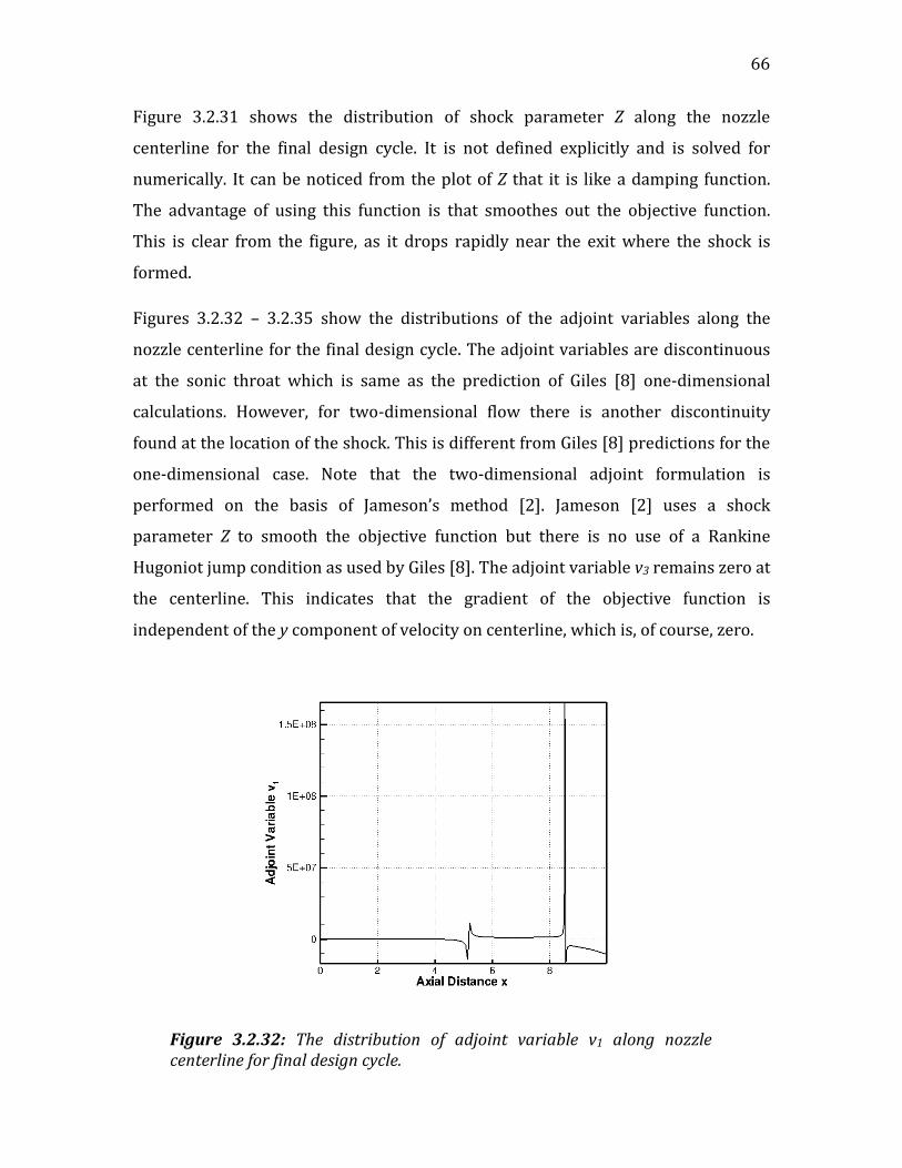
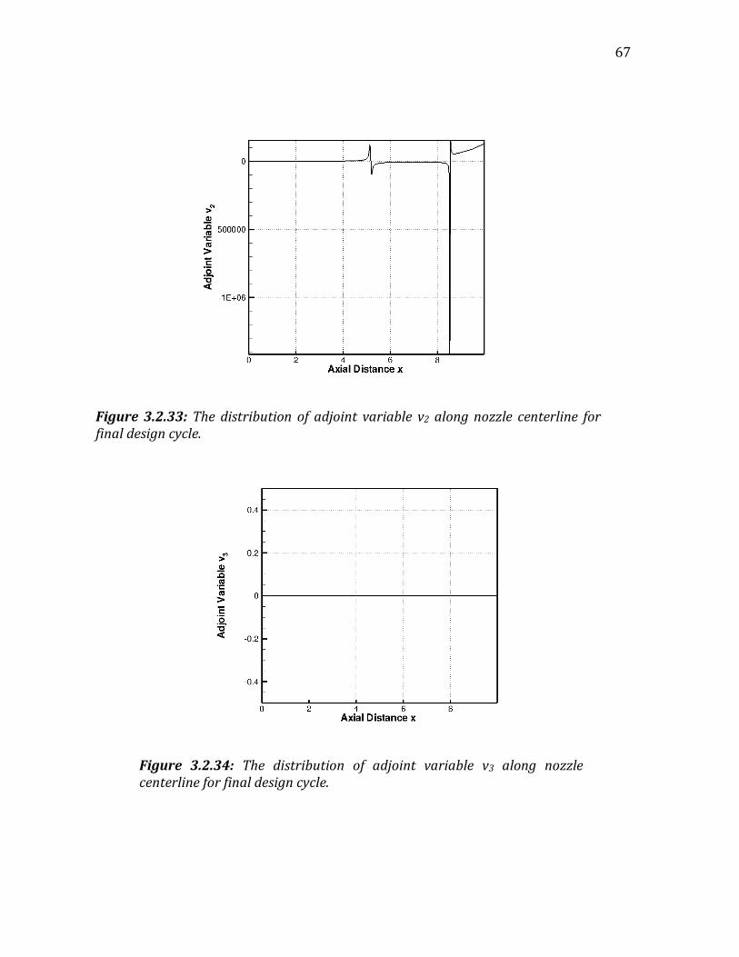
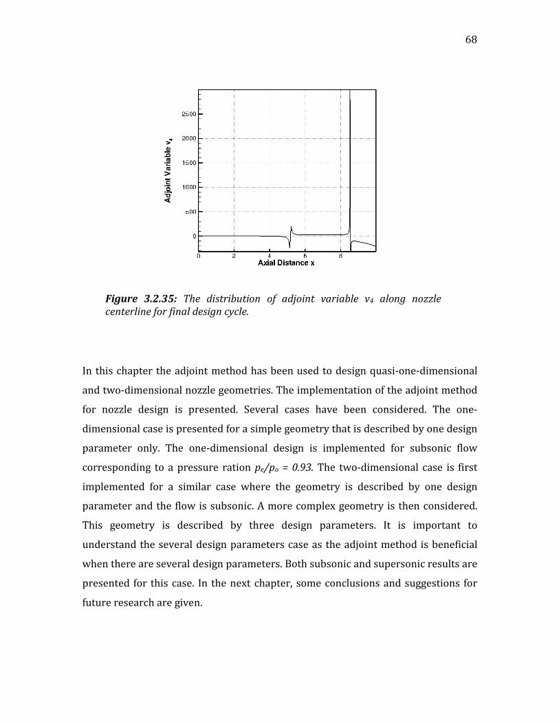
Figures 3.2.32 – 3.2.35 show the distributions of the adjoint variables along the

nozzle centerline for the final design cycle. The adjoint variables are discontinuous

at the sonic throat which is same as the prediction of Giles [8] one-dimensional

calculations. However, for two-dimensional flow there is another discontinuity

found at the location of the shock. This is different from Giles [8] predictions for the

one-dimensional case. Note that the two-dimensional adjoint formulation is

performed on the basis of Jameson’s method [2]. Jameson [2] uses a shock

parameter Z to smooth the objective function but there is no use of a Rankine

Hugoniot jump condition as used by Giles [8]. The adjoint variable v3 remains zero at

the centerline. This indicates that the gradient of the objective function is

independent of the y component of velocity on centerline, which is, of course, zero.

Figure 3.2.32: The distribution of adjoint variable v1 along nozzle centerline for final design cycle.

67

Figure 3.2.34: The distribution of adjoint variable v3 along nozzle centerline for final design cycle.

Figure 3.2.33: The distribution of adjoint variable v2 along nozzle centerline for final design cycle.

68

In this chapter the adjoint method has been used to design quasi-one-dimensional

and two-dimensional nozzle geometries. The implementation of the adjoint method

for nozzle design is presented. Several cases have been considered. The one-

dimensional case is presented for a simple geometry that is described by one design

parameter only. The one-dimensional design is implemented for subsonic flow

corresponding to a pressure ration pe/po = 0.93. The two-dimensional case is first

implemented for a similar case where the geometry is described by one design

parameter and the flow is subsonic. A more complex geometry is then considered.

This geometry is described by three design parameters. It is important to

understand the several design parameters case as the adjoint method is beneficial

when there are several design parameters. Both subsonic and supersonic results are

presented for this case. In the next chapter, some conclusions and suggestions for

future research are given.

Figure 3.2.35: The distribution of adjoint variable v4 along nozzle centerline for final design cycle.

69

Chapter4: Conclusion and Future Work

Adjoint methods have been shown to be very efficient methods of optimization in

terms of saving computational cost. In this thesis, adjoint methods have been

developed for quasi-one-dimensional and two-dimensional nozzle flows. The aim is

to find a geometry that has an optimum value corresponding to a desired cost

function. The cost function, in this thesis, has been considered as the difference of

the pressure distribution from a desired pressure distribution on the nozzle axis.

The adjoint variables are used to find the sensitivity of the cost function with

respect to the design parameters. First, a quasi-one-dimensional case is considered

to explain the method. Then more complicated two-dimensional cases are

considered. The two-dimensional cases have been demonstrated for a one design

parameter case for understanding purposes and then a several design parameters

two-dimensional case has been considered. The nozzle operating conditions include

both subsonic and supersonic cases. In the supersonic case, when there is a shock

present in the nozzle, the cost function has been smoothed. Even though the cost

function has been smoothed for the supersonic case, the adjoint variables are

observed to be discontinuous at the sonic throat and at the location of the shock.

The number of design cycles required to achieve the desired pressure distribution

varies with the type of problem (subsonic, supersonic), and type of governing

equations (quasi-one-dimensional, two-dimensional). The adjoint equation is

similar to the flow equation. Hence its solution takes approximately the same

computational effort as the flow equation. Traditional methods of computing the

cost function sensitivity require much more computational effort with a new flow

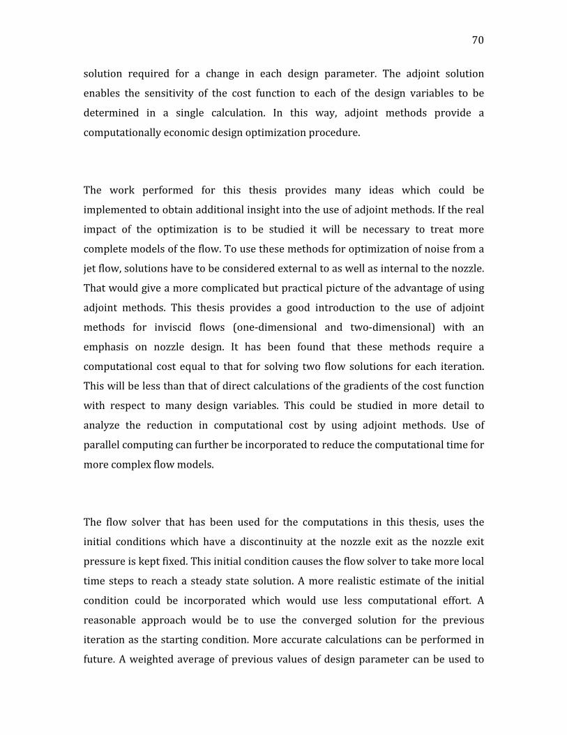
70

solution required for a change in each design parameter. The adjoint solution

enables the sensitivity of the cost function to each of the design variables to be

determined in a single calculation. In this way, adjoint methods provide a

computationally economic design optimization procedure.

The work performed for this thesis provides many ideas which could be

implemented to obtain additional insight into the use of adjoint methods. If the real

impact of the optimization is to be studied it will be necessary to treat more

complete models of the flow. To use these methods for optimization of noise from a

jet flow, solutions have to be considered external to as well as internal to the nozzle.

That would give a more complicated but practical picture of the advantage of using

adjoint methods. This thesis provides a good introduction to the use of adjoint

methods for inviscid flows (one-dimensional and two-dimensional) with an

emphasis on nozzle design. It has been found that these methods require a

computational cost equal to that for solving two flow solutions for each iteration.

This will be less than that of direct calculations of the gradients of the cost function

with respect to many design variables. This could be studied in more detail to

analyze the reduction in computational cost by using adjoint methods. Use of

parallel computing can further be incorporated to reduce the computational time for

more complex flow models.

The flow solver that has been used for the computations in this thesis, uses the

initial conditions which have a discontinuity at the nozzle exit as the nozzle exit

pressure is kept fixed. This initial condition causes the flow solver to take more local

time steps to reach a steady state solution. A more realistic estimate of the initial

condition could be incorporated which would use less computational effort. A

reasonable approach would be to use the converged solution for the previous

iteration as the starting condition. More accurate calculations can be performed in

future. A weighted average of previous values of design parameter can be used to

71

calculate the next value of design parameter. Different geometries and different

numbers of the design parameters can be studied to obtain a better indication of the

benefits of the method. It would also help in understanding the limitations of the

method. A two-dimensional nozzle has been considered in this thesis for most of

the calculations. However, to examine more practical cases an axisymmetric nozzle

could be considered and use of the adjoint method could be applied to that case.

72

References

1. “Aerodynamic design via control theory” Jameson, A., J. Sci. Comput.3 (1988)

233-260.

2. “Optimum Aerodynamic design using CFD and control theory” Jameson, A., AIAA95-1729-CP (1995).

3. “Optimum aerodynamic design using control theory” Jameson, A., In: Hafez, M. and Oshima, K. (eds), Computational Fluid Dynamics Review, Annual Book Series. John Wiley & Sons, New York (1995) pp. 495-528.

4. “Optimum aerodynamic design using Navier-Stokes equations” Jameson, A., Pierce, N.A. and Martinelli, L., AIAA Paper 97-0101 (1997).

5. “Control based airfoil design using the Euler equations” Reuther, J., and Jameson, A., AIAA Paper 94-4272-CP (1994).

6. “Aerodynamic shape optimization of complex aircraft configurations via an adjoint formulation” Reuther, J., Jameson, A., Farmer, J., Martinelli, L., and Saunders, D., AIAA Paper 96-0094 (1996).

7. “An Introduction to the Adjoint Approach to Design” M. B. Giles and N. A. Pierce, Flow, Turbulence and combustion 65: 393-415, (2000).

8. “Analytic adjoint solutions for the quasi-one-dimensional Euler equations” M. B. Giles and N. A. Pierce, J. Fluid Mechanics (2001), vol. 426, pp. 327-345.

9. “On the Properties of Solutions of the Adjoint Euler Equations” M. B. Giles and N. A. Pierce

10. “The noise from shock waves in supersonic jets” Harper-Bourne, M. and Fisher, M.J., AGARD-CP-131 11:1-13 (1974).

11. “Stochastic model theory of broadband shock associated noise from supersonic jets,” Tam, C.K.W., J. Sound Vib 116, 265-302 (1987).

12. “Optimal Control of Systems Governed by Partial Differential Equations”

Lions, J.L., Springer- Verlag, Berlin (1971). Translated by S.K. Mitter.

73

13. “On optimum design in fluid mechanics” Pironneau O., J. Fluid Mech. 64

(1974) 97–110.

14. “Adjoint operator approach to shape design for internal incompressible flow” Cabuk, H., Shung, C.H. and Modi, V., In: Dulikravich, G.S. (ed.), Proceedings 3rd International Conference on Inverse Design and Optimization in Engineering Sciences (1991) pp. 391–404.

15. “Sensitivity analysis, approximate analysis and design optimization for internal and external viscous flows” Korivi, V.M., Taylor III, A.C. and Hou, G.W., AIAA Paper 91-3083 (1991).

16. “Aerodynamics design and optimization in one shot” Ta’asan, S., Kuruvila, G.

and Salas, M.D., AIAA Paper 92-0025 (1992).

17. “Aerodynamic design optimization using sensitivity analysis and computational fluid dynamics” Baysal, O. and Eleshaky, M.E., AIAA J. 30(3) (1992) 718–725.

18. “Practical design and optimization in computational fluid dynamics”

Huffman, W.P., Melvin, R.G., Young, D.P., Johnson, F.T., Bussoletti, J.E., Bieterman, M.B. and Himes, C.L., AIAA Paper 93-3111 (1993).

19. “Airfoil design via control theory using the full-potential and Euler

equations” Lewis, J. and Agarwal, R., The Forum on CFD for Design and Optimization (IMECE 95), San Francisco, CA (1995).

20. “Aerodynamic design optimization on unstructured grids with a continuous adjoint formulation” Anderson, W.K. and Venkatakrishnan, V., AIAA Paper 97-0643 (1997).

21. “CFD design problems using progressive optimization” Dadone, A. and

Grossman, B., AIAA Paper 99-3295 (1999).

22. “Overview of sensitivity analysis and shape optimization for complex aerodynamic configurations” Newman III, J.C., Taylor III, A.C., Barnwell, R.W., Newman, P.A. and Hou, G.J.-W., J. Aircraft 36(1) (1999) 87–96.

23. “Aerodynamic optimization based on the Euler and Navier–Stokes equations using unstructured grids” Elliott, J., Ph.D. Thesis, MIT, Department of Aeronautics and Astronomy (1998).

24. “Aerodynamic design optimization on unstructured meshes using the Navier–Stokes equations” Nielsen, E. and Anderson, W.K., AIAA Paper 98-

74

4809 (1998).

25. “Airfoil design on unstructured grids for turbulent flows” Anderson, W.K. and Bonhaus, D.L., AIAA J. 37(2) (1999) 185–191.

26. “Optimal shape design, reverse mode of automatic differentiation and turbulence” Mohammadi, B., AIAA Paper 97-0099 (1997).

27. “Computational Fluid Dynamics: The basics with applications” Anderson J.

D., McGraw Hill international editions.

75

Nomenclature

U = flow properties vector

u = perturbation in flow properties

p = pressure

q = one-dimensional velocity

ρ = density

E = energy

H = enthalpy

h = nozzle half height (one-dimensional)

˜ h = perturbation in h

pd = desired pressure

v = adjoint variable

Jc = jacobian

ξ,η( ) = transformed coordinates

α = design parameter

J = objective function

I = sensitivity of objective function with respect to design parameter

Z = shock parameter

Cx, Cy = coefficients of artificial dissipation