ISCTE - Instituto Universitário de Lisboa

BRU-IUL (Unide-IUL)

Av. Forças Armadas

1649-126 Lisbon-Portugal

http://bru-unide.iscte.pt/

FCT Strategic Project UI 315 PEst-OE/EGE/UI0315

Working Paper Working Paper Working Paper Working Paper –––– 11113333/0/0/0/07777

The Use And Misuse Of Structural The Use And Misuse Of Structural The Use And Misuse Of Structural The Use And Misuse Of Structural Equation Modeling In Management Equation Modeling In Management Equation Modeling In Management Equation Modeling In Management ResearchResearchResearchResearch

Nebojša St. DavNebojša St. DavNebojša St. DavNebojša St. Davčikikikik

1

THE USE AND MISUSE OF STRUCTURAL EQUATION MODELING IN

MANAGEMENT RESEARCH

Dr. Nebojša St. Davčik

ISCTE Business School, University Institute of Lisbon (ISCTE-IUL),

Assistant Professor of Marketing

&

BRU Research Fellow

davcik@live.com; nebojsa.davcik@iscte.pt

Av. Das Forcas Armadas, 1649-026, Lisbon, Portugal

Abstract: The research practice in management research is dominantly based on structural equation

modeling, but almost exclusively, and often misguidedly, on covariance-based SEM. We adumbrate

theoretical foundations and guidance for the two SEM streams: covariance-based, also known as LISREL,

covariance structure analysis, latent variable analysis, etc.; and variance-based SEM, also known as a

component-based SEM, PLS, etc. Our conceptual framework discusses the two streams by analysis of

theory, measurement model specification, sample and goodness-of-fit. We question the usefulness of

Cronbach’s alpha research paradigm and discuss alternatives that are well-established in social science, but

not well-known in the management research community. We conclude with discussion of some open

questions in management research practice that remain under-investigated and unutilized.

Keywords: Structural equation modeling, covariance- and variance-based SEM, formative and reflective

indicators, LISREL, PLS

JEL classification: C18, C3, M0

Acknowledgements: The author is grateful to Oriol Iglesias, Jonas Rundquist, Ming Lim, Fathima Saleem

and Zoran Cajka for insightful comments and suggestions on previous versions of this manuscript. I had

valuable technical support from Verica Beslic. All mistakes and misunderstandings are the author’s.

2

THE USE AND MISUSE OF STRUCTURAL EQUATION MODELING IN

MANAGEMENT RESEARCH

1. INTRODUCTION

Structural equation models (SEM) with

unobservable variables are a dominant research

paradigm in the management community today,

even though it originates from the psychometric

(covariance-based, LISREL; hereinafter

CBSEM) and chemometric research tradition

(variance-based, PLS; hereinafter VBSEM). The

establishment of the covariance-based SEM

approach can be traced back to the development

of the maximum likelihood covariance structure

analysis developed by Jöreskog (1966, 1967,

1969, 1970, 1973, 1979) and extended by Wiley

(1973). The origins of the PLS approach,

developed by Herman Wold, can be traced back

to 1963 (Wold 1975, 1982). The first procedures

for single- and multi-component models have

used least squares (LS), and later Wold (1973)

extended his procedure several times under

different names: NIPLS (nonlinear iterative

partial least square) and NILES (nonlinear

iterative least square).

Management measures in self-reporting

studies are based almost exclusively (e.g.,

Diamantopoulos & Winklhofer 2001;

Diamantopoulos et al. 2008) on creating a scale

that is assumed reflective and further analysis is

dependent on a multitrait-multimethod (MTMM)

approach and classical test theory, which implies

application of a covariance-based structural

equation model (CBSEM). A partial least square

(PLS) approach, which was introduced in

management literature by Fornell and Bookstein

(1982), is another statistical instrument; but so

far this approach has not had a wider application

in management literature and research practice.

The use of PLS for index construction purposes

is an interesting area for further research

(Diamantopoulos & Winklhofer 2001; Wetzels et

al. 2009) and with new theoretical insights and

software developments it is expected that this

approach will have wider acceptance and

application in the management community.

After reading and reviewing a great number of

studies (articles, books, studies, etc.) that apply

SEM, as well as analyzing a great number of

academic articles (e.g., Boomsma 2000; Chin

1998a; Diamantopoulos et al. 2008; Finn &

Kayande 2005; Tomarken & Waller 2005), it has

become obvious that many researchers apply this

statistical procedure without a comprehensive

understanding of its basic foundations and

principles. Researchers often fail in application

and understanding of (i) conceptual background

of the research problem under study, which

should be grounded in theory and applied in

management; (ii) indicator - construct

misspecification design (e.g., Chin 1998b; Jarvis

et al. 2003; MacKenzie 2001; MacKenzie et al.

2005); (iii) an inappropriate use of the necessary

measurement steps, which is especially evident in

the application of CBSEM (indices reporting,

competing models, parsimonious fit, etc.) and

(iv) an inaccurate reporting of the sample size

and population under study (cf. Baumgartner &

Homburg 1996; Boomsma 2000).

The study that thoroughly analyzes, reviews

and presents two streams using common

methodological background. There are examples

in the literature that analyze two streams (e.g.

Chin 1998b; Petter et al. 2007; Henseler et al.

2009; Wetzels et al. 2009; Hair et al. 2010; cf.

Anderson & Gerbing 1988), but previous studies

take a partial view, analyzing one stream and

3

focusing on the differences and advantages

between the two streams. Fornell and Bookstein

(1982) have demonstrated in their empirical

study many advantages of PLS over LISREL

modeling, especially underlying the differences

in measurement model specification, in which

reflective constructs are associated with LISREL

(CBSEM), whereas formative and mixed

constructs are associated with PLS (VBSEM).

From the present perspective, the study of

Fornell and Bookstein makes a great historical

contribution because it was the first study that

introduced and analyzed the two streams in

management research. Unfortunately,

management theory and practice remained almost

exclusively focused on the CBSEM application.

Their study has somewhat limited theoretical

contribution because they focused only on

differences in the measurement model

specification between the two streams. We focus

on the correct model specification with respect to

the theoretical framework, which is a crucial

aspect of the model choice in SEM. Our intention

is to extend the conceptual knowledge that

remained unexplored and unutilized. Our paper is

as minimally technical as possible, because our

intention is not to develop new research avenues

at this point, but to address possible theory

enhancements and gaps in extant management

research practice (cf. Yadav 2010).

The purpose of this article is two-fold: (i) to

question the current research myopia in

management, because application of the latent

construct modeling almost blindly adheres only a

covariance-based research stream; and (ii) to

improve the conceptual knowledge by comparing

the most important procedures and elements in

the structural equation modeling (SEM) study,

using different theoretical criteria. We present the

covariance-based (CBSEM) and variance-based

(VBSEM) structural equation modeling streams.

The manuscript is organized into several

sections. First, we discuss a general approach to

structural equation modeling and its applicability

in management research. Second, we discuss the

two SEM streams in detail, depicted in Table 1,

and followed by an analysis of topics such as

theory, model specification, sample and

goodness-of-fit. The remaining part of the paper

is devoted to conclusions and some open

questions in management research practice that

remain under-investigated and unutilized.

2. COVARIANCE-BASED AND

VARIANCE-BASED STRUCTURAL

EQUATION MODELING

Structural models in management are

statistical specifications and estimations of data

and economic and/or management theories of

consumer or firm behavior (cf. Chintagunta et al.

2006). Structural modeling tends to explain

optimal behavior of agents and to predict their

future behavior and performances. By behavior

of agents, we mean consumer utility, employee

performances, profit maximizing and

organizational performances by firms, etc. (cf.

Chintagunta et al. 2006). SEM is a statistical

methodology that undertakes a multivariate

analysis of multi-causal relationships among

different, independent phenomena grounded in

reality. This technique enables the researcher to

assess and interpret complex interrelated

dependence relationships as well as to include the

measurement error on the structural coefficients

(Hair et al. 2010, MacKenzie 2001; Steenkamp &

Baumgartner 2000). Byrne (1998) has advocated

that structural equation modeling has two

statistical pivots: (i) the causal processes are

represented by a series of structural relations; and

(ii) these equations can be modeled in order to

conceptualize the theory under study. SEM can

4

be understood as theoretical empiricism because

it integrates theory with method and observations

(Bagozzi 1994). Hair et al. (2010, p. 616) have

advocated that SEM examines “the structure of

interrelationships expressed in a series of

equations”. These interrelationships depict all of

the causality among constructs, the exogenous as

well as endogenous variables, which are used in

the analysis (Hair et al. 2010).

Two SEM streams have been recognized in

modern research practice. The first one is the

“classical” SEM approach – also known by

different names including covariance structure

analysis and latent variable analysis – which

utilizes software such as LISREL or AMOS

(Hair et al. 2010; Henseler et al. 2009). We will

call this stream covariance-based SEM (CBSEM)

in this manuscript. For most researchers in

marketing and business research, CBSEM “is

tautologically synonymous with the term SEM”

(Chin 1998b, p. 295). Another stream is known

in the literature as partial least squares (PLS) or

component-based SEM (e.g., Henseler et al.

2009; McDonald 1996; Tenenhaus 2008; Hwang

2010). This stream is based on application of

least squares using the PLS algorithm with

regression-based methods or generalized

structured component analysis (GSCA), which is

a fully informational method that optimizes a

global criterion (Tenenhaus 2008; Hwang et al.

2010). This stream will be named the variance-

based SEM (VBSEM) in this text.

The rationale behind this notation is grounded

on the following three characteristics:

i) Basic specification of the

structural models is similar, although

approaches differ in terms of their model

development procedure, model

specification, theoretical background,

estimation and interpretation (cf. Hair et al.

2010).

ii) VBSEM intends to explain

variance, i.e. prediction of the construct

relationships (Fornell & Bookstein 1982;

Hair et al. 2010; Hair et al. 2012); CBSEM

is based on the covariance matrices; i.e.

this approach tends to explain the

relationships between indicators and

constructs, and to confirm the theoretical

rationale that was specified by a model.

iii) Model parameters differ in two

streams. The variance-based SEM is

working with component weights that

maximize variance, whereas the

covariance-based SEM is based on factors

that tend to explain covariance in the model

(cf. Fornell & Bookstein 1982).

We present Table 1 below; in the remainder of

this section, the two streams will be described in

detail, using topics such as theory, model

specification, sample and goodness-of-fit.

Interested readers can use Table 1 as a

framework and guide throughout the manuscript.

2.1. Theory

Academic research is grounded in theory,

which should be confirmed or rejected, or may

require further investigation and development.

Hair et al. (2010, p. 620) have argued, “a model

should not be developed without some

underlying theory”, and this process includes

measurement and underlying theory (Fornell

1983; cf. Bagozzi 1983). Without proper

measurement theory, the researcher cannot

develop adequate measures and procedures to

estimate the proposed model.

5

Table 1: Structural equation modeling: CBSEM & VBSEM

TOPIC S E M

COVARIANCE (CBSEM) VARIANCE (VBSEM)

Th

eory

Theory background strictly theory driven based on theory, but data driven

Relation to the theory confirmatory predictive

Research orientation parameter prediction

Mo

del

sp

ecif

icat

ion

Type of the latent measures

(constructs)

reflective indicators (and formative, if identified by

reflective) reflective and/or formative indicators

Latent variables factors components

Model parameters factor means component weights

Type of study psychometric analysis (attitudes, purchase intention, etc.)

drivers of success, organizational constructs (market /

service / consumer orientation, sales force, employees,

etc.)

Structure of unobservables indeterminate determinate

Reliability measures Cronbach’s α (and / or Guttman’s λ and GLB)

a) Cohen’s ƒ2

b) ρc indicator or Cronbach’s α, Guttman’s λ and

GLB (for the reflective models only)

Input data covariance / correlation matrix individual-level raw data

Sam

ple

Sample size ratio of sample size to free model parameters – minimum 5

observations to 1 free parameter, optimum is 10

a) Ten observations multiplied with the construct that

has highest number of indicators

b) The endogenous construct with the largest number

of exogenous constructs, multiplied with ten

observations

Data distribution assumption identical distribution “soft” modeling , identical distribution is not assumed

Go

od

nes

s-o

f-fi

t

Assessment of the model fit

a) Overall (absolute) fit measures

b) Comparative (incremental) fit measures

c) Model parsimony

a) Model predictiveness (coefficient of

determination, Q2 predictive relevance and average

variance extracted – AVE)

b) Stability of estimates, applying the resampling

procedures (jack-knifing and bootstrapping).

Residual co/variance residual covariances are minimized for optimal parameter

fit

residual variances are minimized to obtain optimal

prediction

Software LISREL, AMOS, etc. SmartPLS, SPSS (PLS module), etc.

6

Furthermore, the researcher cannot provide

proper interpretation of the hypothesized model,

there are no new theoretical insights and overall

theoretical contribution is dubious without

underlying theory (cf. Bagozzi & Phillips 1982).

However, there is an important difference in

theory background between CBSEM and

VBSEM. CBSEM is considered a confirmatory

method that is guided by theory, rather than by

empirical results, because it tends to replicate

the existing covariation among measures

(Fornell & Bookstein 1982; Hair et al. 2010;

Reinartz et al. 2009; cf. Anderson & Gerbing

1988; Diamantopoulos & Siguaw 2006; Fornell

1983; Wetzels et al. 2009), analyzing how

theory fits with observations and reality.

CBSEM is strictly theory driven, because of the

exact construct specification in measurement

and structural model as well as necessary

modification of the models during the

estimation procedure (Hair et al. 2010; cf.

Fornell 1983; Rigdon 2005); “the chi square

statistic of fit in LISREL is identical for all

possible unobservables satisfying the same

structure of loadings, a priori knowledge is

necessary” (Fornell & Bookstein 1982, p. 449).

VBSEM is also based on some theoretical

foundations, but its goal is to predict the

behavior of relationships among constructs and

to explore the underlying theoretical concept.

From a statistical point of view, VBSEM reports

parameter estimates that tend to maximize

explained variance, similarly to OLS regression

procedure (Fornell & Bookstein 1982; Anderson

& Gerbing 1988; Diamantopoulos & Siguaw

2006; Hair et al. 2010; Hair et al. 2012; cf.

Wetzels et al. 2009; Reinartz et al. 2009;

Rigdon 2005). Therefore, VBSEM is based on

theory, but is data driven in order to be

predictive and to provide knowledge and new

theoretical rationale about the researched

phenomenon. According to Jöreskog and Wold

(1982), CBSEM is theory oriented and supports

the confirmatory approach in the analysis, while

VBSEM is primarily intended for predictive

analysis in cases of high complexity and small

amounts of information.

There is one important distinction regarding

the research orientation between the two

streams. Residual covariances in CBSEM are

minimized in order to achieve parameter

accuracy, however for VBSEM, residual

variances “are minimized to enhance optimal

predictive power” (Fornell & Bookstein 1982,

p. 443; cf. Bagozzi 1994; Chin 1998; Yuan et al.

2008). In other words, the researcher tends to

confirm theoretical assumptions and accuracy of

parameters in CBSEM; in contrast, the

predictive power of the hypothesized model is

the main concern in VBSEM.

2.2. Specification of the measurement model

The vast majority of management research

includes self-reported studies of consumer

behavior, attitudes and/or opinions of managers

and employees, which express the proxy for

different behavioral and organizational

relationships in business reality. A researcher

develops a model that is a representation of

different phenomena connected with causal

relationships in the real world. In order to

provide a theoretical explanation of these

behavioral and/or organizational relationships,

the researcher has to develop complex research

instruments that will empirically describe

theoretical assumptions about researched

phenomenon. This process is named the

measurement model specification (Fornell &

Bookstein 1982; Hair et al. 2010; Rossiter

2002).

A measure is an observed score obtained via

interviews, self-reported studies, observations,

7

etc. (Edwards & Bagozzi 2000; Howell et al.

2007). It is a quantified record that represents an

empirical analogy to a construct. In other words,

a measure is quantification of the material

entity. A construct in measurement practice

represents a conceptual entity that describes

manifest and/or latent phenomenon as well as

their interrelationships, outcomes and

performances. Constructs themselves are not

real (or tangible) in an objective manner, even

though they refer to real-life phenomena

(Nunnally & Bernstein 1994). In other words,

the relationship between a measure and a

construct represents the relationship between a

measure and the phenomenon, in which the

construct is a proxy for the phenomena that

describe reality (cf. Edwards & Bagozzi 2000).

Throughout this paper, we use the terms

“measure” and “indicator” interchangeably to

refer to a multi-item operationalization of a

construct, whether it is reflective or formative.

The terms “scale” and “index” should be used to

distinguish between reflective and formative

items respectively (Diamantopoulos & Siguaw

2006).

Academic discussions about the relationships

between measures and constructs are usually

based on examination of the causality among

them. The causality of the reflective construct is

directed from the latent construct to the

indicators, with the underlying hypothesis that

the construct causes changes in the indicators

(Fornell & Bookstein 1982; Edwards & Bagozzi

2000; Jarvis et al. 2003). Discussions of

formative measures indicate that a latent

variable is measured using one or several of its

causes (indicators), which determine the

meaning of that construct (e.g., Blalock 1964;

Edwards & Bagozzi 2000; Jarvis et al. 2003).

Between the reflective and formative constructs

exists an important theoretical and empirical

difference, but many researchers do not pay

appropriate attention to this issue and

mistakenly specify the wrong measurement

model. According to Jarvis et al. (2003),

approximately 30% of the latent constructs

published in the top management journals were

incorrectly specified. The model ramification

included incorrect specification of the reflective

indicators when they should have been

formative indicators, at not only the first-order

construct level but also the relationships

between higher-order constructs (Jarvis et al.

2003; cf. Petter et al. 2007). Using the Monte

Carlo simulation, they have demonstrated that

the misspecification of indicators can cause

biased estimates and misleading conclusions

about the hypothesized models (cf. Yuan et al.

2008). The source of bias is mistakenly

specified due to the direction of causality

between the measures and latent constructs,

and/or the application of an inappropriate item

purification procedure (Diamantopoulos et al.

2008). The detailed descriptions and

applications of the reflective and formative

constructs are presented in the following

subsection.

The latent variables in CBSEM are viewed as

common factors, whereas in VBSEM they are

considered as components or weighted sums of

manifest variables. This implies that latent

constructs in the VBSEM approach are

determinate, whereas in the CBSEM approach

they are indeterminate (Chin 1998b; cf. Fornell

& Bookstein 1982). The consequence is the

specification of model parameters as factor

means in CBSEM, whereas in VBSEM they are

specified as component weights (cf. Rigdon

2005; Reinartz et al. 2009). Factors in the

CBSEM estimates explain covariance, whereas

component weights maximize variance because

they represent a linear combination of their

indicators in the latent construct (Fornell &

Bookstein 1982). Several researchers have

examined the relationships between latent and

manifest variables (e.g., Bagozzi 2007; Howell

8

et al. 2007). They have suggested that the

meaning of epistemic relationships between the

variables should be established before its

inclusion and application within a nomological

network of latent and manifest variables.

The researcher can use single and multiple

measures to estimate the hypothesized

constructs. Researchers usually use multiple

measures because (i) most constructs can be

measured only with an error term; (ii) a single

measure cannot adequately capture the essence

of the management phenomena (cf. Curtis &

Jackson 1962); (iii) it is necessary to prove that

the method of measurement is correct (Nunnally

& Bernstein 1994; MacKenzie et al. 2005); and

(iv) it is necessary to use a minimum of three

indicators per construct in order to be able to

identify a model in the CBSEM set-up (cf.

Anderson & Gerbing 1988; Bollen 1989b;

Baumgartner & Homburg 1996). When multiple

measures are developed, the researcher has to

estimate the model that accurately, validly and

reliably represents the relationship between

indicators and latent constructs in the structural

model. Research bias may arise if the researcher

uses very few indices (three or less), or fails to

use a large number of indicators for each latent

construct (cf. Chin 1998b; Peter 1979); so-

called “consistency at large”. In the VBSEM

technique, consistency at large means that

parameters of the latent variable model and the

number of indicators are infinite (Wold 1980;

McDonald 1996; cf.; Reinartz et al. 2009;

Rigdon 2005).

The structural constructs (i.e.,

multidimensional constructs, hierarchical

constructs; cf. Fornell & Bookstein 1982; Law

et al. 1998; McDonald 1996; Wetzels et al.

2009; Bagozzi 1994; Chintagunta et al. 2006)

represent multilevel inter-relationships among

the constructs that involve several exogenous

and endogenous interconnections and include

more than one dimension. The researcher should

distinguish higher-order models from a model

that employs unidimensional constructs that are

characterized by a single dimension among the

constructs. The literature (cf. Fornell &

Bookstein 1982; Chin 1998b; Diamantopoulos

& Winklhofer 2001; MacKenzie et al. 2005;

Tenenhaus et al. 2005; Wetzels et al. 2009, etc.)

recognize three types of structural constructs:

the common latent construct model with

reflective indicators, the composite latent

construct model with formative indicators, and

the mixed structural model.

2.2.1. Types of latent constructs

The simplified structural models with the

reflective and/or formative constructs are

represented in Figures 1, 2 and 3. A circle or

ellipsis represents an unobserved or latent

variable; a square represents an observed or

manifest variable (cf. Bagozzi & Phillips 1982).

An arrow that indicates a direction between a

circle and square represents the effects of a

latent variable on its measure in the first order

reflective construct and, vice versa, the effects

of a manifest variable on a latent variable in the

first-order formative construct.

These figures use “classical” SEM notation

that needs some attention. ξ (ksi) represents a

latent construct associated with observed xi

indicators, η (eta) stands for a latent construct

associated with observed yi indicators, the error

terms δi (delta) and εi (epsilon) are associated

with observed xi and yi indicators, respectively.

ζ (zeta) is the error term associated with the

formative construct. λij represents factor loading

in the i-th observed indicator that is explained

by the j-th latent construct. γij represents weight

in the i-th observed indicator that is explained

by the j-th latent construct. A detailed

description is provided in Table 2.

9

Table 2: Summary of abbreviations and descriptions used in the SEM study

Symbol Name Description

ξ ksi A latent construct associated with observed xi

indicators

η eta A latent construct associated with observed yi

indicators

δi delta The error term associated with observed xi indicators

εi epsilon The error term associated with observed yi indicators

ζ zeta The error term associated with formative construct

λij lambda factor loading in the i-th observed indicator that is

explained by the j-th latent construct

γij gamma weight in the i-th observed indicator that is explained

by the j-th latent construct

xi An indicator associated with exogenous construct, i.e.

vector of observed exogenous variable

yi An indicator associated with endogenous construct,

i.e. vector of observed endogenous variable

Table 3 represents common topics and

criteria for the distinction between reflective

and formative indicators. Common topics are

grouped according to two criteria: i) the

construct-indicator relationship; and ii)

measurement. The construct-indicator

relationship topic is discussed via employing

criteria such as direction of causality, theoretical

framework, definition of the latent construct,

common antecedents and consequences, internal

consistency, validity of constructs and indicator

omission consequences. The measurement topic

is discussed by analyzing the issue of

measurement error, interchangeability,

multicollinearity and a nomological net of

indicators.

Figure 1 depicts the “classical” SEM case

where the model is specified in the reflective

mode. The type A case depicts a path diagram

between the two latent constructs (ξ –

exogenous and η – endogenous), with three

indicators per construct (xi and yi). This case

can be represented by equations 1 and 2:

(1) xi = λijξ + δi

(2) yi = λijη + εi

This specification assumes that the error term

is unrelated to the latent variable COV(η, εi) =

0, and independent COV(εi, εj) = 0, for i ≠ j and

expected value of error term E(εi) = 0. This type

of model specification is typical for the classical

test theory and factor analysis models (Fornell

& Bookstein 1982; Bollen & Lennox 1991;

Chin 1998b; Diamantopoulos & Winklhofer

2001) used in behavioral studies.

10

Table 3: Indicators: Reflective indicators (RI) & Formative indicators (FI)

TOPICS Indicators

REFLECTIVE (RI) FORMATIVE (FI)

The

const

ruct

– i

ndic

ator

rela

tionsh

ip

Direction of causality from the construct to the measure (indicator) from the measure (indicator) to the construct

Theoretical framework (type of the

constructs) psychometric constructs (attitudes, personality, etc.)

organizational constructs (marketing mix, drivers of

success, performances, etc.)

The latent construct is empirically

defined common variance total variance

The indicators relationship to the same

antecedents and consequences required not required

Internal consistency reliability implied not implied

Validity of constructs internal consistency reliability nomological and / or criterion-related validity

Indicator omission from the model does not influence the construct may influence the construct

Number of indicators per construct minimum 3

i) In VBSEM: Conceptually dependent

ii) In CBSEM: min 3 formative, with 2 reflective

for identification

Mea

sure

men

t

Measurement error at the indicator level at the construct level

Interchangeability expected not expected

Multicollinearity expected not expected

Development of the multi-item

measures scale index

Nomological net of the indicators should not differ may differ

11

Application of the classical test theory “assumes

that the variance in scores on a measure of a

latent construct is a function of the true score

plus error” (MacKenzie et al. 2005, p. 710;

Podsakoff et al. 2003), as we presented in

equations 1 and 2. The rationale behind the

reflective indicators is that they all measure the

same underlying phenomenon (Chin 1998b) and

they should account for observed variances and

covariances (Fornell & Bookstein 1982; cf.

Edwards 2001) in the measurement model. The

meaning of causality has direction from the

construct to the measures with underlying

assumptions that each measure is imperfect

(MacKenzie et al. 2005), i.e., that has the error

term which can be estimated at the indicator

level.

Figure 1 – Type A: Latent constructs with

reflective indicators

Figure 2 – Type B: Latent constructs with

formative indicators

The type B model specification, presented in

Figure 2, is known as a formative (Fornell &

Bookstein 1982; cf. Edwards 2001) or causal

indicator (Bollen and Lennox 1991), because

the direction of causality goes from the

indicators (measures) to the construct and the

error term is estimated at the construct level.

This type of model specification can be

represented by equations 3 and 4:

(3) ξ = γijxi + ζ

(4) η = γijyi + ζ

This specification assumes that the indicators

and error term are not related, i.e. COV(yi, ζ) =

0, and E(ζ) = 0 . Formative indicators were

introduced for the first time by Curtis and

Jackson (1962) and extended by Blalock (1964).

This type of model specification assumes that

the indicators have an influence on (or that they

cause) a latent construct. In other words, the

indicators as a group “jointly determine the

conceptual and empirical meaning of the

construct” (Jarvis et al. 2003, p. 201; cf.

Edwards & Bagozzi 2000). The type B model

specification would give better explanatory

power, in comparison to the type A model

specification, if the goal is the explanation of

unobserved variance in the constructs (Fornell

& Bookstein 1982; cf. McDonald 1996).

Application of the formative indicators in the

CBSEM environment is limited by necessary

additional identification requirements. A model

is identified if model parameters have only one

group of values that create the covariance

matrix (Gatignon 2003). In order to resolve the

problem of indeterminacy that is related to the

construct-level error term (MacKenzie et al.

2005), the formative-indicator construct must be

associated with unrelated reflective constructs.

This can be achieved if the formative construct

emits paths to i) at least two unrelated reflective

indicators; ii) at least two unrelated reflective

constructs; and iii) one reflective indicator that

is associated with a formative construct and one

reflective construct (MacKenzie et al. 2005; cf.

12

Fornell & Bookstein 1982; Diamantopoulos &

Winklhofer 2001; Diamantopoulos et al. 2008;

Edwards & Bagozzi 2000; Howell et al. 2007;

Bagozzi 2007; Wilcox et al. 2008).

From an empirical point of view, the latent

construct captures (i) the common variance

among indicators in the type A model

specification; and (ii) the total variance among

its indicators in the type B model specification,

covering the whole conceptual domain as an

entity (cf. Cenfetelli & Bassellier 2009;

MacKenzie et al. 2005). Reflective indicators

are expected to be interchangeable and have a

common theme. Interchangeability, in the

reflective context, means that omission of an

indicator will not alter the meaning of the

construct. In other words, reflective measures

should be unidimensional and they should

represent the common theme of the construct

(e.g., Petter et al. 2007; Howell et al. 2007).

Formative indicators are not expected to be

interchangeable, because each measure

describes a different aspect of the construct’s

common theme, and dropping an indicator will

influence the essence of the latent variable (cf.

Bollen & Lenox 1991; Coltman et al. 2008;

Diamantopoulos & Winklhofer 2001;

Diamantopoulos et al. 2008; Jarvis et al. 2003).

The behavior of measures of the construct with

regards to the same antecedents and

consequences is an important criterion for the

assessment of the construct-indicator

relationship. Reflective indicators are

interchangeable, which means that measures are

affected by the construct, and they must have

the same antecedents and consequences. The

formative constructs are affected by the

measures, thus are not necessarily

interchangeable, and each measure can

represent a different theme. For the formative

indicators it is not necessary to have the same

antecedents and consequences (cf. Bollen 2007;

Coltman et al. 2008; Howell et al. 2007; Jarvis

et al. 2003; Petter et al. 2007).

Internal consistency is implied within the

reflective indicators, because measures must

correlate. High correlations among the reflective

indicators are necessary, because they represent

the same underlying theoretical concept. This

means that all of the items are measuring the

same phenomenon within the latent construct

(Petter et al. 2007; MacKenzie et al. 2005). On

the contrary, within the formative indicators,

internal consistency is not implied because the

researcher does not expect high correlations

among the measures (cf. Jarvis et al. 2003).

Because formative measures are not required to

be correlated, validity of construct should not be

assessed by internal consistency reliability as

with the reflective measures, but with other

means such as nomological and/or criterion-

related validity (cf. Bollen & Lenox 1991;

Coltman et al. 2008; Diamantopoulos et al.

2008; Jarvis et al. 2003; Bagozzi 2007).

The researcher should ascertain the

difference of multicollinearity between the

reflective and formative constructs. In the

reflective-indicator case, multicollinearity does

not represent a problem for measurement-model

parameter estimates, because the model is based

on simple regression (cf. Fornell & Bookstein

1982; Bollen & Lenox 1991; Diamantopoulos &

Winklhofer 2001; Jarvis et al. 2003) and each

indicator is by purpose collinear with other

indicators. However, high inter-correlations

among the indicators are a serious issue in the

formative-indicator case, because it is

impossible to identify the distinct effect of an

indicator on the latent variable (cf.

Diamantopoulos & Winklhofer 2001;

MacKenzie et al. 2005; Cenfetelli & Bassellier

2009). The researcher can control for indicator

collinearity by assessing the size of the

tolerance statistics (1 - ), where

is the

13

coefficient of the determination in predicting

variable Xj (cf. Cenfetelli & Bassellier 2009).

Inverse expression of the tolerance statistics is

the variance inflation factor (VIF), which has

different standards of threshold values that

range from 3.33 to 10.00, with lower values

being better (e.g., Diamantopoulos & Siguaw

2006; Hair et al 2010; Cenfetelli & Bassellier

2009).

The multi-item measures can be created by

the scale developed or the index construction.

Traditional scale development guidelines will be

followed if the researcher conceptualizes the

latent construct as giving rise to its indicators,

and therefore viewed as reflective indicators to

the construct. This procedure is based on the

intercorrelations among the items, and focuses

on common variance, unidimensionality and

internal consistency (e.g., Diamantopoulos &

Siguaw 2006; Anderson & Gerbing 1982;

Churchill 1979, Nunnally & Bernstein 1994).

The index development procedure will be

applied if the researcher conceptualizes the

indicators as defining phenomenon in relation to

the latent construct, and therefore will be

considered as formative indicators of the

construct. Index construction is based on

explaining unobserved variance, considers

multicollinearity among the indicators and

underlines the importance of indicators as

predictor rather than predicted variables (e.g.,

Diamantopoulos & Siguaw 2006; Bollen 1984;

Diamantopoulos & Winklhofer 2001;

MacCallum & Browne 1993).

The mixed case is represented by Figure

3. The researcher can create a model that uses

both formative and reflective indicators. It is

possible for a structural model to have one type

of latent construct at the first-order (latent

construct) level and a different type of latent

construct at the second-order level (Fornell &

Bookstein 1982; MacKenzie et al. 2005;

Diamantopoulos & Siguaw 2006; Wetzels et al.

2009).

Figure 3 – Type C: Latent constructs with

reflective and formative indicators

In other words, the researcher can combine

different latent constructs to form a hybrid

model (Edwards & Bagozzi 2000; McDonald

1996; Tenenhaus et al. 2005). Development of

this model type depends on the underlying

causality between the constructs and indicators,

as well as the nature of the theoretical concept.

The researcher should model exogenous

constructs in the formative mode and all

endogenous constructs in the reflective mode,

(i) if one intends to explain variance in the

unobservable constructs (Fornell & Bookstein

1982; cf. Wetzels et al. 2009); and (ii) in case of

weak theoretical background (Wold 1980).

Conducting a VBSEM approach in this model,

using a PLS algorithm, is equal to redundancy

analysis (Fornell et al. 1988; cf. Chin 1998b),

because the mean variance in the endogenous

construct is predicted by the linear outputs of

the exogenous constructs.

2.2.2. Reliability assessment

The scale development paradigm was

established by Churchill’s (1979) work as seen

in the management measurement literature. This

management measurement paradigm has been

investigated and improved by numerous

14

research studies and researchers, with special

emphasis on the reliability and validity of

survey research indicators and measures (e.g.,

Peter 1981; Anderson & Gerbing 1982; Fornell

& Bookstein 1982; Churchill & Peter 1984;

Finn & Kayande 2004, etc.). Any quantitative

research must be based on accuracy and

reliability of measurement (Cronbach 1951). A

reliability coefficient demonstrates the accuracy

of the designed construct (Cronbach 1951; cf.

Churchill & Peter 1984) in which certain

collection of items should yield interpretation

regarding the construct and its elements.

It is highly likely that no other statistic has

been reported more frequently in the literature

as a quality indicator of test scores than

Cronbach’s (1951) alpha coefficient (Sijtsma

2009; Shook et al. 2004). Although Cronbach

(1951) did not invent the alpha coefficient, he

was the researcher who most successfully

demonstrated its properties and presented its

practical applications in psychometric studies.

The invention of the alpha coefficient should be

credited to Kuder and Richardson (1937), who

developed it as an approximation for the

coefficient of equivalence, and named it rtt(KR20);

and Hoyt (1941), who developed a method of

reliability based on dichotomous items, for

binary cases where items are scored 0 and 1 (cf.

Cronbach 1951; Sijtsma 2009). Guttman (1945)

and Jackson and Ferguson (1941) also

contributed to the development of Cronbach’s

version of the alpha coefficient, by further

development of data derivations for Kuder and

Richardson’s rtt(KR20) coefficient, using the same

assumptions but without stringent expectations

on the estimation patterns. The symbol α was

introduced by Cronbach (1951, p. 299) “… as a

convenience. ‘Kuder-Richardson Formula 20’ is

an awkward handle for a tool that we expect to

become increasingly prominent in the test

literature”. Cronbach’s α measures how well a

set of items measures a single unidimensional

construct. In other words, Cronbach’s α is not a

statistical test, but a coefficient of an item’s

reliability and/or consistency. The most

commonly accepted formula for assessing the

reliability of a multi-item scale could be

represented by:

(5) (

) (

∑

)

where N represents the item numbers, is

the variance of the item i and represents the

total variance of the scale (cf. Cronbach 1951;

Peter 1979; Gatignon 2003). In the standardized

form, alpha can be calculated as a function of

the total items correlations and the inter-item

correlations:

(6)

( )

where N is item numbers, c-bar is the

average item-item covariance and v-bar is the

average variance (cf. Gerbing & Anderson

1988). From this formula it is evident that items

are measuring the same underlying construct, if

the c-bar is high. This coefficient refers to the

appropriateness of item(s) that measure a single

unidimensional construct. The recommended

value of the alpha range is from 0.6 to 0.7 (Hair

et al. 2010; cf. Churchill 1979; Petter 1979), but

in academic literature a commonly accepted

value is higher than 0.7 for a multi-item

construct and 0.8 for a single-item construct.

Academic debate on the pales and usefulness

of several reliability indicators, among them

Cronbach’s α, is unabated in the psychometric

arena, but this debate is practically unknown

and unattended in the management community.

The composite reliability, based on a coefficient

alpha research paradigm, cannot be a unique

assessment indicator because it is limited by its

research scope (Finn & Kayande 1997) and is

an inferior measure of reliability (Baumgartner

& Homburg 1996). Alpha is a lower bound to

15

the reliability (e.g., Guttman 1945; Jackson &

Agunwamba 1977; Ten Berge & Sočan 2004;

Sijtsma 2009) and is an inferior measure of

reliability in most empirical studies

(Baumgartner & Homburg 1996). Alpha is the

reliability if variance is zero for all i-th ≠ j-th,

which implies essential τ-equivalence among

the items, but this limitation is not very common

in practice (Novick & Lewis 1967; Ten Berge &

Sočan 2004; Sijtsma 2009).

We shall now discuss several alternatives to

the alpha coefficient that are not well-known in

practical applications and the management

community. The reliability of the test score X in

the population is denoted by ρxx’. It is defined as

the product-moment correlation between scores

on X and the scores on parallel test scores X’

(Sijtsma 2009). From the psychometric studies,

we have a well-known:

(7) 0 ≤ ρxx’ ≤ 1

and

(8) ρxx’ = 1 –

where represents variance of the random

measurement error and represents variance

of the test score. It is evident from equation (8)

that the reliability can be estimated if (i) two

parallel versions of the test are analyzed; and

(ii) the error variance is available (Sijtsma 2009;

Gatignon 2003). These conditions are not

possible in many practical applications. Several

reliability coefficients have been proposed as a

better solution for the data from a single test

administrator (Guttman 1945; Nunnally &

Bernstein 1994; Sijtsma 2009), such as the GLB

and Guttman’s λ4 coefficient.

The greatest lower bound (GLB)

represents the largest value of an indicator that

is smaller than each of the indicators in a set of

constructs. The GLB solution holds by finding

the nonnegative matrix CE that is positive

semidefinite (PSD):

(9) GLB = 1 – ( )

( )

where CE represents the inter-item error

covariance matrix. Equation (9) represents the

GLB under the limitation that the sum of error

variances correlate zero with other indicators

(Sijtsma 2009), because it is the greatest

reliability that can be obtained using an

observable covariance matrix.

Guttman’s λ4 reliability coefficient is

based on the split-half lower bounds paradigm.

The difference between Guttman’s λ4 and the

traditional “corrected” split-half coefficient is

that it uses estimation without assumptions of

equivalence. The split-half lower bound to

reliability, with assumption of experimentally

independent parts (Guttman 1945), is defined by

(10) λ4 = n (

)

where σ2

i and σ2

j represent the respective

variances of the independent parts and n

represents the number of parts to be estimated.

Guttman (1945) has proved that λ4 is a better

coefficient in comparison to the traditional

“corrected” split-half coefficient, and that alpha

coefficient, in Guttman (1945) notated as λ3, is

lower bound to λ4.

The relationships among different

reliability indicators are:

(11) 0 ≤ alpha (λ3) ≤ λ4 ≤ GLB ≤ ρxx’ ≤ 1

This expression is true, because we

know from Guttman (1945) that alpha (λ3) ≤ λ4,

from Jackson and Agunwamba (1977) that λ4 ≤

GLB, and from Ten Berge and Sočan (2004)

that GLB ≤ ρxx’ ≤ 1. The alpha and Guttman’s λ

can be estimated using the SPSS, and the GLB

can be calculated by the program MRFA2 (Ten

16

Berge & Kiers 2003; cf. Ten Berge & Kiers

1991), which is available from

www.ppsw.rug.nl/~kiers/.

From a research point of view the composite

reliability, based on Cronbach’s so-called alpha

indicator, cannot solely be an assessment

indicator because it is limited by its scope only

on the scaling of person, rather than on the

scaling of objects such as firms, advertisements,

brands, etc. (e.g., Peter 1979; Finn & Kayande

1997). The generalizability theory (G-theory)

introduced by Cronbach and colleagues (1963,

1972) and measured by the coefficient of

generalizability includes wider management

facets and takes into account many sources of

error in a measurement procedure. The G-theory

represents a multifaceted application of

measurement (Cronbach et al. 1972; Peter 1979;

Finn & Kayande 1997) that generalizes over the

scaling of persons in the population and focuses

on the scaling of objects such as organizations,

brands, etc. The measurement in G-theory is

conducted by variation from multiple

controllable sources, because random effects

and variance elements of the model are

associated with multiple sources of variance

(Peter 1979; Finn & Kayande 1997). The

coefficient of generalizability is defined by the

estimate of the expected value of ρ2 (Cronbach

et al. 1972):

(12) E 2 =

where σ2

us represents the variance component

related to an object of measurement, and σ2

re

represents the sum of variance that affects the

scaling of the object of measurement. This

measure has no wider application in the

management community due to its robust

measurement metrics and high cost. There is

some evidence in the literature (e.g., Finn &

Kayande 1997) that a piece of such research,

with 200 respondents, may cost approximately

10,000 US$ (as of 1995).

In summary, researchers should be aware

that conventional reporting of the alpha

coefficient has empirical and conceptual

limitations. We recommend that authors should

make additional efforts to report Guttman’s λ

(from SPSS, same as alpha) together with the

alpha coefficient. Application of the GLB

coefficient in management practice will be

highly appreciated and rewarded.

Cohen’s ƒ2. The researcher can evaluate a

VBSEM model by assessing the R-squared

values for each endogenous construct. This

procedure can be conducted because the case

values of the endogenous construct are

determined by the weight relations (Chin

1998b). The change in R-squares will show the

influence of an individual exogenous construct

on an endogenous construct. The effect size ƒ2

has been used as a reliability measure in the

VBSEM applications, but researchers do not

address properly the role of effect size effects in

the model. It is usual practice to report this

effect directly from statistical program (such as

SmartPlS), but this is not an automatic function

and statistical power of the model must be

calculated additionally. This indicator is

proposed by Cohen (1988) and can be

“calculated as the increase in R2 relative to the

proportion of variance of the endogenous latent

variable that remains unexplained” (Cohen

1988; 1991; cf. Chin 1998b). To estimate the

overall effect size of the exogenous construct,

the following formula can be used:

(13)

–

Another way to calculate this indicator is

with a power analysis program such as GPower

3.1. The researcher can easily estimate effect

size ƒ2 using partial R-squares (Faul et al. 2007;

17

2009). Cohen (1988; 1991) has suggested that

values of 0.02, 0.15 and 0.35 have weak,

medium or large effects, respectively.

Composite reliability ρc indicator. The

VBSEM models in reflective mode should

apply the composite reliability ρc measure or

Cronbach’s α (and/or Guttman’s λ4 and GLB),

as a control for internal consistency. The

composite reliability ρc indicator was developed

by Werts, Linn and Jöreskog (1974) and can be

interpreted in the same way as Cronbach’s α

(Chin 1998b; Henseler et al. 2009). This

procedure applies the normal partial least square

output, because it standardizes the indicators

and latent constructs (Chin 1998b).

(14) (∑ )

(∑ ) ∑ ( )

where λij represents the component loading

on an indicator by the j-th latent construct and

Var(εij) = 1 – λij2. The ρc has more accurate

parameter estimates in comparison to

Cronbach’s α, because this indicator does not

assume tau equivalency among the constructs.

Werts et al. (1974) have argued that the

composite reliability ρc is more appropriate to

apply to VBSEM applications than Cronbach’s

α, because Cronbach’s α may produce serious

underestimation of the internal consistency of

latent constructs. This is the case because

Cronbach’s α is based on the assumption that all

indicators are equally reliable. The partial least

square procedure ranks indicators according to

their reliability (Henseler et al. 2009) and makes

them a more reliable measure in the VBSEM

application. The composite reliability ρc is only

applicable in the latent constructs with reflective

measures (Chin 1998b).

Table 4: Preferred value of the Cronbach’s Alpha, ρc indicator, Guttman’s λ, GLB and Cohen’s ƒ-

square indicators

Cronbach’s α & ρc indicator (and /

or Guttman’s λ and GLB) Cohen’s ƒ-square

Preferred value

i) 0.60 – 0.70 for multi-item

constructs (minimum)

ii) ≥ 0.70 preferred for multi-item

constructs

iii) ≥ 0.80 for single-item constructs

(minimum)

i) 0.02 – weak effect

ii) 0.15 – medium effect

iii) 0.35 – strong effect

2.2.3. Validity assessment

The ongoing discussion in the measurement

literature (e.g., Rossiter 2002, 2005;

Diamantopoulos & Siguaw 2006; Finn &

Kayande 2005) on procedures for the

development of scales and indexes to measure

constructs in management is beyond the scope

of this manuscript. We only want to draw

attention at this point to the validity and

reliability of applied constructs. Validation

represents the process of obtaining the scientific

evidence for a suggested interpretation of

quantitative results from a questionnaire by the

researcher.

In research practice, validity is very often

assessed together with reliability. This process

18

represents the extent to which a measurement

concept obtains consistent estimations. From a

statistical point of view, test validity represents

the degree of correlation between the model and

statistical criterion. The validity procedure has

gained greater importance in SEM application

than in other statistical instruments, because i)

this procedure makes an important distinction

between the measurement and the structural

model; and ii) this application provides a more

stringent test of discriminant validity, construct

reliability, etc. (e.g., Bagozzi 1980; Fornell &

Larcker 1981; Gerbing & Anderson 1988; Jarvis

et al. 2003; cf. Peter 1979; Rossiter 2002).

Construct validity is a necessary condition

for testing the hypothesized model (Gerbing &

Anderson 1988), because “construct validity

pertains to the degree of correspondence

between constructs and their measures” (Peter

1981, p. 133; cf. Curtis & Jackson 1962;

Bagozzi & Phillips 1982). In other words,

construct validity represents the extent to which

operationalizations of a latent construct

measures the underlying theory. Evidence of

construct validity represents empirical support

for the theoretical interpretation of the

constructs. The researcher must assess the

construct validity of the model, without which

one cannot estimate and correct for the

influences of measurement errors that may

deteriorate the estimates of theory testing

(Bagozzi & Phillips 1982; Bagozzi et al. 1991).

However, researchers must be aware that

construct validity is applicable only with

reflective constructs. The fidelity of formative

measures in CBSEM, except in some limited

cases such as concurrent or predictive validity

(Bagozzi 2007), is hard to assess and difficult to

justify in terms of the conceptual meaning of a

model.

Discriminant validity represents the

distinctive difference among the constructs. In

other words, discriminant validity shows the

degree to which the indicators for each of the

constructs are different from each other (cf.

Churchill 1979; Bagozzi & Phillips 1982). The

researcher can assess the discriminant validity

by examining the level of correlations among

the measures of independent constructs. A low

intra-construct correlation is a sign of

discriminant validity. The average variance

extracted (AVE) for each construct should be

greater than squared correlations among the

measures of a construct in order to ensure the

discriminant validity (Fornell & Larcker 1981).

Nomological aspects of validation include

connecting the index to other constructs with

which it should be connected, for instance,

antecedents and/or consequences

(Diamantopoulos & Winklhofer 2001; Jarvis et

al. 2003; cf. Gerbing & Anderson 1988; Law et

al. 1998). Nomological validity can be assessed

by estimating the latent construct and testing

whether correlations between antecedents and

consequences are significantly higher than zero

(MacKenzie et al. 2005). This validation is

especially important when certain indicators are

eliminated from the constructs and the

researcher has to establish whether new

constructs behave in an expected way. In other

words, the nomological net of indicators should

not differ in the reflective mode and may differ

in the formative mode (e.g., Bollen & Lenox

1991; Jarvis et al. 2003).

2.2.4. Type of study

The management studies that investigate

organizational constructs, such as

market/consumer orientation, sales force, etc.,

and drivers of success are by their nature theory

predictive rather than theory confirmatory

studies. These constructs are determined by a

combination of factors that cause specific

19

phenomenon and their indicators should be

created in a formative mode (Fornell &

Bookstein 1982; Chin 1998b). This implies that

this type of study is better with VBSEM, but

decisions about the approach should be made

after careful examination of all elements that

influence the two streams.

However, behavioral studies that are based

on psychometric analysis of factors such as

attitudes, consumer intentions, etc., are seen as

underlying factors that confirm a specific

theory. They “give rise to something that is

observed” (Fornell & Bookstein 1982, p. 442)

and should be created in a reflective mode. The

researcher should start the conceptual

examination from the CBSEM point of view.

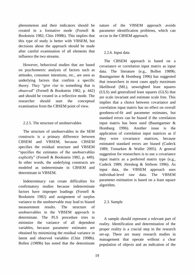
2.2.5. The structure of unobservables

The structure of unobservables in the SEM

constructs is a primary difference between

CBSEM and VBSEM, because CBSEM

specifies the residual structure and VBSEM

“specifies the estimates of the unobservables

explicitly” (Fornell & Bookstein 1982, p. 449).

In other words, the underlying constructs are

modeled as indeterminate in CBSEM and

determinate in VBSEM.

Indeterminacy can create difficulties for

confirmatory studies because indeterminate

factors have improper loadings (Fornell &

Bookstein 1982) and assignment of surplus

variance to the unobservable may lead to biased

measurement results. The structure of

unobservables in the VBSEM approach is

determinate. The PLS procedure tries to

minimize the variance of all dependent

variables, because parameter estimates are

obtained by minimizing the residual variance in

latent and observed variables (Chin 1998b).

Bollen (1989b) has noted that the determinate

nature of the VBSEM approach avoids

parameter identification problems, which can

occur in the CBSEM approach.

2.2.6. Input data

The CBSEM approach is based on a

covariance or correlation input matrix as input

data. The literature (e.g., Bollen 1989b;

Baumgartner & Homburg 1996) has suggested

that researchers in most cases apply maximum

likelihood (ML), unweighted least squares

(ULS) and generalized least squares (GLS) that

are scale invariant and estimate scale free. This

implies that a choice between covariance and

correlation input matrix has no effect on overall

goodness-of-fit and parameter estimates, but

standard errors can be biased if the correlation

input matrix has been used (Baumgartner &

Homburg 1996). Another issue is the

application of correlation input matrices as if

they were covariance matrices, because

estimated standard errors are biased (Cudeck

1989; Tomarken & Waller 2005). A general

suggestion for researchers is to use a covariance

input matrix as a preferred matrix type (e.g.,

Cudeck 1989; Jöreskog & Sörbom 1996). As

input data, the VBSEM approach uses

individual-level raw data. The VBSEM

parameter estimation is based on a least square

algorithm.

2.3. Sample

A sample should represent a relevant part of

reality. Identification and determination of the

proper reality is a crucial step in the research

set-up. There are many research studies in

management that operate without a clear

population of objects and an indication of the

20

sample size under study. For instance, a

researcher studies the problem of innovation in

management. He/she conducts (or attempts to

conduct) interviews with a great number of

managers (>1000) from different industries,

different management levels, different positions

in companies, and different working and life

experience and expectations. The first issue is

that of objective reality. What does the

researcher study? The great population

diversification leads to an inconsistent sample

and biased estimation about the researched

phenomenon, because of very heterogeneous

variables (industry, position, experience, etc.).

The second issue is sampling. Identifying the N-

number of respondents to which the researcher

can send his/her questionnaire is not the reality

he/she wants to investigate. The researcher

wants to indentify the sample that is a

representative part of objective reality. In the

self-reported studies, which deal with cross-

sectional data, the acceptable threshold level is

15% (Hair et al. 2010).

The researcher should consider the following

two questions regarding the appropriateness of

the employed sample size and model. Firstly,

what is the proper sample size, in comparison to

the number of observations, which will

represent business reality? Secondly, what is the

appropriate number of indicators to be

estimated, in comparison with the obtained

sample size, in a proposed model (cf.

Baumgartner & Homburg 1996)?

Sample size of the model differs in two

streams. The importance of sample size lies in

the fact that it serves as a basis for estimation of

the error term and the most important question

is how large a sample must be to obtain credible

results (Hair et al. 2010). There is no general

rule of thumb or formula which can give an

exact solution for the necessary number of

observations in SEM.

The adequate size of a sample in the CBSEM

approach depends on several factors (cf. Hair et

al. 2010; Marcoulides & Saunders 2006) such as

i) multivariate normality; ii) applied estimation

technique (cf. Baumgartner & Homburg 1996),

because there can be applied maximum

likelihood estimation (MLE), weighted least

squares (WLS), generalized least squares

(GLS), asymptotically distribution free (ADF)

estimation, etc. (cf. Jöreskog & Sörbom 1996;

Byrne 1998; Baumgartner & Homburg 1996;

Hu et al. 1992; Sharma et al. 1989); iii) model

complexity, because more complex models

require more observations for the estimation; iv)

missing data, because it reduces the original

number of cases; v) communality in each

construct, i.e. the average variance extracted in

a construct. A great number of simulation

studies on CBSEM (usually the Monte Carlo

simulation) report estimation bias, improper

results and non-convergence problems with

respect to sample size (e.g.; Henseler et al.

2009) and inadequate indicator loadings

(Reinartz et al. 2009). In general, the researcher

can apply the necessary sample size rule,

bearing in mind the above limitations and

suggestions, if the ratio of sample size to free

model parameters is at least five observations to

one free parameter for the minimum threshold

level and ten to one for the optimum threshold

level (Bentler & Chou 1987; cf. Baumgartner &

Homburg 1996; Marcoulides & Saunders 2006;

Hu et al. 1992; Peter 1979). Baumgartner and

Homburg (1996) have shown that the average

ratio of sample size to number of parameters

estimated in management literature (from 1977-

1994) is 6.4 to 1. Interested readers are referred

to MacCallum et al. (2001), Baumgartner and

Homburg (1996) and Hair et al. (2010) for a

more comprehensive discussion.

The VBSEM approach is more robust and

less sensitive to sample size, in comparison to

the CBSEM approach. For instance, Wold

21

(1989) has successfully conducted a study with

10 observations and 27 latent constructs; Chin

and Newsted (1999) have conducted a Monte

Carlo simulation study on VBSEM in which

they have found that the VBSEM approach can

be applied to a sample of 20 observations. In

general, the rule of thumb that researchers can

use in VBSEM runs as follows (Chin 1998b): i)

10 observations multiplied with the construct

that has the highest number of indicators; ii) the

endogenous construct with the largest number

of exogenous constructs, multiplied by ten

observations. However, the researcher should be

careful when employing the small sample size

cases in the VBSEM study, because the PLS

technique is not the silver bullet (cf.

Marcoulides & Saunders 2006) for any level of

sample size, even though it offers “soft”

assumptions on data distribution and sample

size.

2.4. Goodness-of-fit

2.4.1. Goodness-of-fit in VBSEM

A model evaluation procedure in VBSEM is

different in comparison to the CBSEM

approach. The VBSEM application is based on

the partial least squares procedure that has no

distributional assumptions, other than predictor

specification (Chin 1998b). Traditional

parametric-based techniques require identical

data distribution. Evaluation of the VBSEM

models should apply the measures that are

prediction oriented rather than confirmatory

oriented based on covariance fit (Wold 1980;

Chin 1998b).

The researcher has to assess a VBSEM

model evaluating the model predictiveness

(coefficient of determination, Q2 predictive

relevance and average variance extracted –

AVE) and the stability of estimates applying the

resampling procedures (jack-knifing and

bootstrapping).

Assessment of the VBSEM model starts with

evaluation of the coefficient of determination

(R2) for the endogenous construct. The

procedure is based on the case values of the

endogenous constructs that are determined by

the weight relations and interpretation is

identical to the classical regression analysis

(Chin 1998b). For instance, Chin (1998b, p.

337) has advocated that the R-squared values

0.63, 0.33 and 0.19, in the baseline model

example, show substantial, moderate and weak

levels of determination, respectively.

The second element of the VBSEM

assessment is that of predictive relevance,

measured by the Q-squared indicator. The Q2

predictive relevance indicator is based on the

predictive sample reuse technique originally

developed by Stone (1974) and Geisser (1975;

1974). The VBSEM adaptation of this approach

is based on a blindfolding procedure that

excludes a part of the data during parameter

estimation and then calculates the excluded part

using the estimated parameters. In other words,

this procedure uses a block of N cases and M

indicators and takes out a part of the N by M

data points. The estimation is conducted by

using the omission distance d in which every d

data point is excluded and calculated separately.

This continues until the procedure reaches the

end of the data matrix (cf. Wold 1982; Chin

1998b).

The predictive relevance indicator is

represented by:

(15) ∑

∑

where Q2 represents a fit between observed

values and values reconstructed by the model.

The sum of squares of prediction errors (SSE)

22

represents the estimated values after the data

points were omitted. The sum of squares of

observations (SSO) represents the mean value

for prediction. Q2 values above zero (Q

2>0)

indicate that observed values are well

reconstructed and a model has predictive

relevance; Q2

values below zero (Q2<0) indicate

that observed values are poorly reconstructed

and that the model has no predictive relevance

(Fornell & Bookstein 1982; Chin 1998b;

Henseler et al. 2009). The relative impact of the

predictive relevance can be assessed by the q2

indicator. This measure can be calculated:

(16) q2 = (Q

2 / 1 – Q

2)

where Q2

represents the above-presented

predictive relevance. The assessed variables of

the model reveal a small impact of the

predictive relevance if q2 ≤ .02, a medium

impact of the predictive relevance if q2 has a

value between .02 and .15; and a strong impact

of the predictive relevance if q2 ≥ .35. Interested

readers are referred to Wold (1982), Fornell and

Bookstein (1982) and Chin (1998b) for further

discussion.

The average variance extracted (AVE)

represents the value of variance captured by the

construct from its indicators relative to the value

of variance due to measurement errors in that

construct. This measure has been developed by

Fornell and Larcker (1981). The AVE is only

applicable for type A models; i.e. models with

reflective indicators, just as in the case of the

composite reliability measure (Chin 1998b).

The average variance extracted ρη for the

construct can be calculated as (Fornell &

Larcker 1981):

(17) ∑

∑ ∑ ( )

where λi is the component loading to an

indicator and Var(εi) = 1 – λi2. If the average

variance extracted ρη is bigger than 0.50, the

variance due to measurement error is smaller

than the variance captured by the construct η,

and validity of the individual indicator (yi) and

construct (η) is well-established (Fornell &

Larcker 1981). The AVE should be higher than

0.50, i.e. more than 50% of variance should be

captured by the model.

VBSEM parameter estimates are not efficient

as CBSEM parameter estimates and resampling

procedures are necessary to obtain estimates of

the standard errors (Anderson & Gerbing 1988).

The stability of estimates in the VBSEM model

can be examined by resampling procedures such

as jack-knifing and bootstrapping. Resampling

estimates the precision of sample statistics by

using the portions of data (jack-knifing) or

drawing random replacements from a set of data

blocks (bootstrapping) (cf. Efron 1979; 1981).

Jack-knifing is an inferential technique used to

obtain estimates by developing robust

confidence intervals (Chin 1998b; Tenenhaus et

al. 2005; Rigdon 2005). This procedure assesses

the variability of the sample data using

nonparametric assumptions and “parameter

estimates are calculated for each instance and

the variations in the estimates are analyzed”

(Chin 1998b, p. 329). Bootstrapping represents

a nonparametric statistical method that obtains

robust estimates of standard errors and

confidence intervals of a population parameter.

In other words, the researcher estimates the

precision of robust estimates in the VBSEM

application.

The procedure described in this section is

useful for the assessment of the structural

VBSEM model. Detailed description and

assessment steps of the outer and inner models

are beyond the scope of this manuscript. Refer

to Chin (1998b), Tenenhaus et al. (2005) and

Henseler et al. (2009) for a more thorough

23

discussion about outer and inner model

assessments.

2.4.2. Goodness-of-fit in CBSEM

CBSEM procedure should be conducted by

the researcher in three phases. The first phase is

the examination of i) estimations of causal

relationships; and ii) goodness-of-fit between

the hypothesized model and observed data. The

second phase involves model modifications in

order to obtain the model with better fit or more

parsimonious estimations. The third phase is

justification that a nested model is superior in

comparison to the original one (cf. Anderson &

Gerbing 1982).

In the first phase, the researcher begins by

examining the estimated value of individual

paths among latent constructs. The statistical

significance of individual path coefficients is

established by the t-values or z-values

associated with structural coefficients

(Schreiber et al. 2006). The second step is

examination of the goodness-of-fit between the

hypothesized model and observed data.

Covariance-based structural equation

modeling has no single statistical test or single

significant threshold that leads to acceptance or

refusal of the model estimations. It is, rather, the

opposite – it has developed a great number of

goodness-of-fit measures that assess the overall

results of the model from different perspectives:

overall fit, comparative fit and model

parsimony. Measures of absolute fit determine

the degree to which the overall model predicts

the observed covariance/correlation matrix

(Hair et al. 2010).

There is no rule of thumb for what model fit

serves as the threshold in covariance-based

structural equation modeling. There are attempts

in the literature (e.g., Bentler & Bonett 1980;

Hu & Bentler 1999; etc.) to obtain “golden

rules”, “silver metrics” or “rules of thumb” for

the assessment of CBSEM. Setting “rules of

thumb” is popular among researchers, because

an established threshold level allows easy and

fast evaluation of the covariance-based models.

The traditional cutoff values in practice, for

incremental fit measures ≥ 0.90, have little

statistical justification and are mostly based on

intuition (Marsh et al. 2004; cf. Baumgartner &

Homburg 1996; Tomarken & Waller 2005).

This issue has also been addressed by Hu and

Bentler (1998, 1999), who have suggested new,

more stringent guidelines. According to these

guidelines, the goodness-of-fit measures should

be evaluated at ≥ 0.95 levels, but researchers

should be aware of possible limitations in the

application and appropriateness of these in

relation to the area of research (e.g.

psychometrics vs. organizational studies) and

the low level of generalizability of this approach

(cf. Marsh & Hau 1996).

Table 5 represents measures of absolute fit,

incremental fit and model parsimony in detail.

For detailed technical assessment and

explanations, interested readers are referred to

Marsh and Hau (1996), Hu and Bentler (1999);

Kenny and McCoach 2003.

Overall (absolute) fit measures (indices). The

researcher can apply several overall fit

measures, such as likelihood-ratio chi statistics,

degrees of freedom, GFI, AGFI, RMSR,

RMSEA, etc. The only statistically based

measure of goodness-of-fit in the CBSEM

application is the likelihood-ratio chi-squared

(χ2) statistic. According to Fornell and Larcker

(1981), the χ2 statistic compares the fit between

the covariance matrices for the observed data

and theoretically created model.

24

Table 5: Measures of absolute fit, incremental fit and model parsimony

Topic Measure Preferred value O

ver

all

fit

mea

sure

s

Chi-square (χ2) 0.05 ≥ p ≤ 0.20

degrees of freedom (df)

no p.v., the researcher uses for

comparative and computational

purposes

Chi-square / df ratio < 2.0

Goodness-of-fit index (GFI) ≥ 0.90

Root mean square residual (RMSR) ≤ 0.08

Root mean square error of

approximation (RMSEA)

no threshold level, practice suggest ≤

0.08

Confidence interval of RMSEA min 90%

Com

par

ativ

e fi

t m

easu

res

Comparative fit index (CFI) 0.0 – 1.0, larger values indicate higher

levels of G-of-F

Incremental fit index (IFI) 0.0 – 1.0, larger values indicate higher

levels of G-of-F

Tucker – Lewis index (TLI / NNFI) ≥ 0.90

Relative non-centrality index (RNI) ≥ 0.90

Relative fit index (RFI) ≥ 0.90

Normed fit index (NFI) ≥ 0.90

Model

par

sim

ony Adjusted goodness-of-fit index (AGFI) ≥ 0.90

Parsimony normed fit index (PNFI) Higher value, better fit

Parsimony ratio ψ 0.0 – 1.0, higher values indicate better

model parsimony

The researcher investigates the non-

significant difference between the actual and

predicted matrices (cf. Fornell 1983; Chin

1998a; Hair et al. 2010; Gatignon 2003),

because the theoretical model strives to account

for all the covariance among the latent

constructs. In other words, we are looking for

the non-significant χ2, which is opposite to

common statistical logic where the researcher is

striving to obtain a model that is statistically

significant at a certain level, usually at 1 or 5%.

Indications that actual and predicted input

covariance matrices are not statistically different

might be obtained if the χ2 value is 0.05 ≥ p ≤

0.20 (Fornell 1983; Hair et al. 2010; Marsh &

Hau 1996; cf. Bagozzi & Phillips 1982). Some

recent studies (e.g., Marsh et al. 2004; Fan &

Sivo 2009) have suggested that χ2 should be

25

used for statistical testing of a model fit, rather

than for descriptive use of a model fit

assessment.

The degrees of freedom (df) of an estimate

are the amount of independent pieces of

information available to estimate a model, i.e.

the number of parameters that are free to vary in

a model. The fundamental difference between

SEM and other statistical techniques is in fact

that df in the SEM application is based on the

size of the covariance matrix (Hair et al. 2010),

which is based on the number of indicators, and

not on the sample size.

The goodness-of-fit index (GFI) is a non-

statistical index that measures the overall degree

of model fit. The fit ranges from very poor

(GFI=0.0) to perfect (GFI=1.0). The adjusted

goodness-of-fit index (AGFI) differs from the

GFI in terms of its adjustment for the number of

degrees of freedom in the model (Byrne 1998).

These two indices can be understood as absolute

indices of fit because they compare the

hypothesized model with no model at all (Byrne

1998) as well as an index of parsimony for the

overstated parameter number and relationships.

Hair et al. (2010) have advocated that higher

values indicate better fit, which in practical

application is accepted as ≥ 0.90 even though

there is no established minimum acceptability

level.

The root mean square residual (RMSR)

represents the average of the residual’s fit

between observed and estimated input matrices

(Hair et al. 2010; Byrne 1998). For this index

there does not exist an official threshold level

(Hair et al. 2010), but in the literature (Byrne

1998) and practice the standardized RMSR ≤

0.08 is established.

The root mean square error of approximation

(RMSEA) is a measure that estimates how well

the population non-centrality index Φ (Steiger

1990) fits to a population covariance matrix per

degrees of freedom (cf. Baumgartner &

Homburg 1996; Yuan 2005) and controls the χ2

statistics to reject models with a large sample or

a large number of variables (cf. Hair et al.

2010). The purpose of the RMSEA in an SEM

study is to adjust the complexity of the model

and sample size. Theory does not advise as to a

generally acceptable threshold value (Feinian et

al. 2008), but in practice the RMSEA ≤ 0.08 is

established. The researcher should take into

consideration the level of the confidence

interval.

Comparative (incremental) fit measures. A

great number of incremental fit measures that

exist in the literature, and that are mostly used

in practical CBSEM applications, are: normed

fit index (NFI), comparative fit index (CFI),

incremental fit index (IFI) and Tucker-Lewis

index (TLI). The normed fit index (Bentler and

Bonett 1980) represents a relative comparison

between a proposed and the null model (Hair et

al. 2010). The fit ranges from very poor

(NFI=0.0) to perfect (NFI=1.0), with preferred

value ≥ 0.90. This index was a “classic”

criterion of model choice in the 1980s, until it

became evident that the NFI underestimated the

model fit in small samples (Byrne 1998).

Bentler (1990) revised the normed fit index and

proposed the comparative fit index (Byrne

1998). The index value has a range of 0.0-1.0,

where larger values indicate higher levels of

goodness-of-fit. The Tucker-Lewis index

(1973), also known as the non-normed fit index

(NNFI), represents a measure of parsimony

between the comparative index in the proposed

and null models (Marsh & Hau 1996; Hair et al.

2010). The TLI estimates a model fit per degree

of freedom, penalizing less parsimonious

models (Baumgartner & Homburg 1996). A

recommended value is ≥ 0.90. The incremental

fit index (Bollen 1989a) describes the

parsimony of the sample size in the estimated

26

and null model. The values lie between 0.0-1.0,

and larger values indicate higher levels of

goodness-of-fit.

Model parsimony. Parsimony of the SEM

model represents comparisons among

competing models, in which the researcher

compares observed model fit relative to its

complexity. A parsimony fit is estimated as the

ratio of degrees of freedom (df) with reference

to the total degrees of freedom (dft) available for

the estimation (Marsh & Balla 1994; Marsh &

Hau 1996). Parsimony ratio is represented by

coefficient ψ:

(19) ψ = dfo / dft

This equation states that the greater the

observed degrees of freedom (dfo) are, the

greater the parsimony ratio will be, which

indicates the better fit of the model (cf. Marsh &

Hau 1996; Kenny & McCoach 2003; Hair et al.

2010). Parsimony fit indices, such as the

adjusted goodness-of-fit index (AGFI) and

parsimony normed fit index (PNFI), tend to

relate model fit to model complexity, which is

similar to the application of an adjusted R2 (Hair

et al. 2010). The PNFI is used as an adjustment

of the normed fit index (NFI). Higher values

represent better fit and model adjustment. The

researcher is advised not to use these indices in

a single model as an independent measure, but

rather as a tool to compare the fit of competing

models.

Competitive fit – Nested models. The primary

goal of an SEM study is to show acceptable

model fit, employing numerous goodness-of-fit

indices, as well as to confirm that the tested

model has no better theoretical alternative.

Assessment of the competing models, which

must be grounded in theory, can be conducted

by comparison using incremental and parsimony

fit measures as well as with differences in the

likelihood-ratio chi-squared statistics when

models are nested. The researcher can compare

models of similar complexity, but with variation

in terms of the underlying theoretical

relationships (Hair et al. 2010; Schreiber et al.

2006; cf. Boomsma 2000; Anderson & Gerbing

1982). If a model contains the same number of

latent constructs as a competing model, and

alters the paths and causality among them, the

researcher can compare nested models by

examining the difference in chi-squared

statistics (Δχ2).

3. RESEARCH ILLUSTRATION

We present recently published research

papers from management literature as an

illustration, which deal with similar research

topic. The idea is to show the contemporary

state of research performance using similar

research topic, but executed by different

researchers that apply various theoretical

assumptions and research approaches. We

present papers on brand loyalty / success

published in the world-known peer reviewed

journals such as Management Decision, Journal

of the Academy of Marketing Science, Journal

of Brand Management, etc. Labrecque et al.

(2011) and Mazodier & Marunka (2011) applied

the CBSEM approach, and Hur et al. (2011) and

Davcik & Rundquist (2012) applied the

VBSEM approach; presented in Table 6.

Labrecque et al. (2011) and Mazodier &

Merunka (2011) applied their research on a

convenient student sample group and a very few

indices per construct (3 – 4), which is a

minimum requirement and gives a good factor

loading.

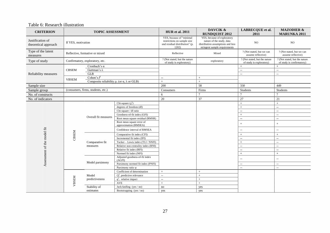
27

Table 6: Research illustration

CRITERION TOPIC ASSESSMENT HUR et al. 2011 DAVCIK &

RUNDQUIST 2012

LABRECQUE et al.

2011

MAZODIER &

MARUNKA 2011

Justification of

theoretical approach If YES, motivation

YES, because of “minimal

restrictions on sample size

and residual distribution” (p.

1202)

YES, because of exploratory

nature of the study, data

distribution assumptions and less

stringent sample requirements

NO NO

Type of the latent

measures Reflective, formative or mixed Reflective Mixed

? (Not stated, but we can

assume reflective)

? (Not stated, but we can

assume reflective)

Type of study Confirmatory, exploratory, etc. ? (Not stated, but the nature

of study is exploratory) exploratory

? (Not stated, but the nature

of study is exploratory)

? (Not stated, but the nature

of study is confirmatory)

Reliability measures CBSEM

Cronbach’s α

+ +

Guttman’s λ -- --

GLB -- --

VBSEM Cohen’s f2 -- +

Composite reliability ρc (or α, λ or GLB) + +

Sample size 200 58 330 449

Sample group (consumers, firms, students, etc.) Consumers Firms Students Students

No. of constructs 6 7 7 7

No. of indicators 20 37 27 21

Ass

essm

ent

of

the

mo

del

fit

CB

SE

M

Overall fit measures

Chi-square (χ2)

+ +

degrees of freedom (df) + --

Chi-square / df ratio -- --

Goodness-of-fit index (GFI) + --

Root mean square residual (RMSR) -- -- Root mean square error of

approximation (RMSEA) + +

Confidence interval of RMSEA -- --

Comparative fit

measures

Comparative fit index (CFI) + +

Incremental fit index (IFI) -- --

Tucker – Lewis index (TLI / NNFI) + --

Relative non-centrality index (RNI) -- --

Relative fit index (RFI) -- --

Normed fit index (NFI) + +

Model parsimony

Adjusted goodness-of-fit index

(AGFI) -- --

Parsimony normed fit index (PNFI) -- --

Parsimony ratio ψ -- --

VB

SE

M Model

predictiveness

Coefficient of determination + +

Q2, predictive relevance -- +

q2, relative impact -- +

AVE + +

Stability of estimates

Jack-knifing (yes / no) no yes

Bootstrapping (yes / no) yes yes

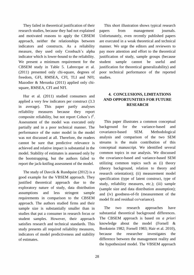
28

They failed in theoretical justification of their

research studies, because they had not explained

and motivated reasons to apply the CBSEM

approach, neither the relationships between

indicators and constructs. As a reliability

measure, they used only Cronbach’s alpha

indicator which is lower-bound to the reliability.

We present a minimum requirement for the

CBSEM study in Table 5. Labrecque et al.

(2011) presented only chi-square, degrees of

freedom, GFI, RMSEA, CFI, TLI and NFI;

Mazodier & Merunka (2011) applied only chi-

square, RMSEA, CFI and NFI.

Hur et al. (2011) studied consumers and

applied a very few indicators per construct (3.3

in average). This paper partly analyses

reliability measures because they report

composite reliability, but not report Cohen’s f2.

Assessment of the model was executed only

partially and in a poor technical manner. The

performance of the outer model in the model

was not discussed at all. Therefore, the readers

cannot be sure that predictive relevance is

achieved and relative impact is substantial in the

model. Stability of estimates is assessed only by

the bootstrapping, but the authors failed to

report the jack-knifing assessment of the model.

The study of Davcik & Rundquist (2012) is a

good example for the VBSEM approach. They

justified theoretical approach due to the

exploratory nature of study, data distribution

assumptions and less stringent sample

requirements in comparison to the CBSEM

approach. The authors studied firms and their

sample size is substantially smaller than in

studies that put a consumer in research focus or

student samples. However, their approach

satisfies research and technical standards. This

study presents all required reliability measures,

indicators of model predictiveness and stability

of estimates.

This short illustration shows typical research

papers from management journals.

Unfortunately, even recently published papers

are executed in a weak theoretical and technical

manner. We urge the editors and reviewers to

pay more attention and effort to the theoretical

justification of study, sample groups (because

student sample cannot be useful and

justification for theoretical generalizability) and

poor technical performance of the reported

studies.

4. CONCLUSIONS, LIMITATIONS

AND OPPORTUNITIES FOR FUTURE

RESEARCH

This paper illustrates a common conceptual

background for the variance-based and

covariance-based SEM. Methodological

analysis and comparison of the two SEM

streams is the main contribution of this

conceptual manuscript. We identified several

common topics in our analysis. We discussed

the covariance-based and variance-based SEM

utilizing common topics such as (i) theory

(theory background, relation to theory and

research orientation); (ii) measurement model

specification (type of latent construct, type of

study, reliability measures, etc.); (iii) sample

(sample size and data distribution assumption);

and (iv) goodness-of-fit (measurement of the

model fit and residual co/variance).

The two research approaches have

substantial theoretical background differences.

The CBSEM approach is based on a priori

knowledge about the model (Fornell &

Bookstein 1982; Fornell 1983; Hair et al. 2010),

because the researcher investigates the

difference between the management reality and

the hypothesized model. The VBSEM approach

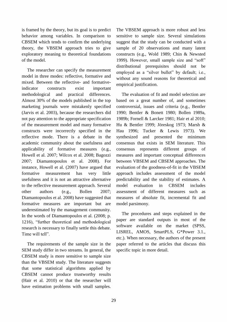
29

is framed by the theory, but its goal is to predict

behavior among variables. In comparison to

CBSEM which tends to confirm the underlying

theory, the VBSEM approach tries to give

exploratory meaning to theoretical foundations

of the model.

The researcher can specify the measurement

model in three modes: reflective, formative and

mixed. Between the reflective- and formative-

indicator constructs exist important

methodological and practical differences.

Almost 30% of the models published in the top

marketing journals were mistakenly specified

(Jarvis et al. 2003), because the researchers did

not pay attention to the appropriate specification

of the measurement model and many formative

constructs were incorrectly specified in the

reflective mode. There is a debate in the

academic community about the usefulness and

applicability of formative measures (e.g.,

Howell et al. 2007; Wilcox et al. 2008; Bagozzi

2007; Diamantopoulos et al. 2008). For

instance, Howell et al. (2007) have argued that

formative measurement has very little

usefulness and it is not an attractive alternative

to the reflective measurement approach. Several

other authors (e.g., Bollen 2007;

Diamantopoulos et al. 2008) have suggested that

formative measures are important but are

underestimated by the management community.

In the words of Diamantopoulos et al. (2008; p.

1216), “further theoretical and methodological

research is necessary to finally settle this debate.

Time will tell”.

The requirements of the sample size in the

SEM study differ in two streams. In general, the

CBSEM study is more sensitive to sample size

than the VBSEM study. The literature suggests

that some statistical algorithms applied by

CBSEM cannot produce trustworthy results

(Hair et al. 2010) or that the researcher will

have estimation problems with small samples.

The VBSEM approach is more robust and less

sensitive to sample size. Several simulations

suggest that the study can be conducted with a

sample of 20 observations and many latent

constructs (e.g., Wold 1989; Chin & Newsted

1999). However, small sample size and “soft”

distributional prerequisites should not be

employed as a “silver bullet” by default; i.e.,

without any sound reasons for theoretical and

empirical justification.

The evaluation of fit and model selection are

based on a great number of, and sometimes

controversial, issues and criteria (e.g., Bentler

1990; Bentler & Bonett 1980; Bollen 1989a,

1989b; Fornell & Larcker 1981; Hair et al 2010;

Hu & Bentler 1999; Jöreskog 1973; Marsh &

Hau 1996; Tucker & Lewis 1973). We

synthesized and presented the minimum

consensus that exists in SEM literature. This

consensus represents different groups of

measures and important conceptual differences

between VBSEM and CBSEM approaches. The

evaluation of the goodness-of-fit in the VBSEM

approach includes assessment of the model

predictability and the stability of estimates. A

model evaluation in CBSEM includes

assessment of different measures such as

measures of absolute fit, incremental fit and

model parsimony.

The procedures and steps explained in the

paper are standard outputs in most of the

software available on the market (SPSS,

LISREL, AMOS, SmartPLS, G*Power 3.1.,

etc.). When necessary, the authors of the present

paper referred to the articles that discuss this

specific topic in more detail.

30

4.1. Some remaining open questions

An important research step is the problem of

reliability. We have presented evidence against

the usage of Cronbach’s alpha in management

studies, because alpha is not an appropriate

reliability indicator, and λ4 and GLB are more

appropriate (e.g., Guttman 1945; Jackson &

Agunwamba 1977; Ten Berge & Sočan 2004;

Sijtsma 2009). The literature is silent about the

behavior of the λ4 and GLB in different

measurement specification contexts. We know

that a researcher can apply these reliability

indicators in the type A mode, but we do not

know whether we can also apply them in modes

B and C. We also do not know if they are

applicable only in the CBSEM set-up, or

whether (and how) we can use them in the

VBSEM set-up. From Werts et al. (1974) we

know that the composite reliability ρc is a better

indicator of reliability than Cronbach’s α in the

VBSEM approach. We do not know what the

theoretical and practical interrelationships are, if

any, among ρc, Guttman’s λ and GLB in the

VBSEM environment. Further software and

theoretical development is needed.

An important issue is further scale

modification, after the management scale has

shown dimensionality and construct validity.

Finn and Kayande (2004) have pointed out that

effects of modified scale on scale performance

is under-investigated in the literature, because

scale adopted to a particular management

context as well as scale refinement are not

covered by classical reliability theory.

Researchers have tried to determine the

minimum sample size needed for a study that

employs the SEM approach, not only in

management but also in other academic fields

(e.g., Bentler & Chou 1987; Baumgartner &

Homburg 1996; Chin 1998b; cf. Marcoulides &

Saunders 2006). For instance, we are not

familiar with any research that questioned or

extended Chin’s “10” rule for a minimum

sample size in the VBSEM environment (cf.

Marcoulides & Saunders 2006). The ongoing

academic debate on how to corroborate the

adequate sample size in both streams needs

further theoretical enhancement and simulation

studies, especially for a heterogeneous

discipline such as management.

The conventional use of SEM employs linear

models on cross-sectional data. There are two

beneficial research avenues not employed in

management. The first is the use of nonlinear

models, such as quadratic effects of exogenous

variables (cf. Steenkamp & Baumgartner 2000)

and Bayesian methods (e.g., Lee 2007; Lee &

Song 2008). On the one hand, this application

can open many new research opportunities for

researchers, but on the other we must be aware

of the limited use of this approach because

variables that employ cross-sectional data are

usually linear. The second beneficial avenue

could be the employment of longitudinal data

and time-series research. The SEM modeling of

time-series data is known in the literature as

latent curve or latent growth modeling.

4.2. Limitations of study

This is a conceptual manuscript and a clear

limitation is an absence of contributions and

discussions based on empirical data. Empirical

simulation, such as the Monte Carlo study, and

an analysis of management data should be a

logical continuation of this topic, but these

enterprises are beyond the scope of this paper

(cf. Tomarken & Waller 2005; Yadav 2010).

The complex CBSEM model that employs

many latent constructs and indices, in three or

31

more layers, is based on a high-dimensional

integration of a parameter that cannot be

efficiently estimated by standard maximum

likelihood methods. The solution might be an

application of Bayesian methods that are based

on Markov Chain Monte Carlo (MCMC)

estimation procedure (cf. Lee 2007).

Management literature is scarce on empirical

simulations and/or studies that analyze and

compare conceptual foundations of covariance-

and variance-based SEM. One of the few

studies that do exist was conducted by Fornell

and Bookstein (1982) almost 30 years ago, but

was limited by their research scope, which

focused only on differences in the measurement

model specification. Tenenhaus (2008) made a

simulation on the ESCI model, using customer

satisfaction data, in which he compared CBSEM

(“classical”, PCA and ULS-SEM) and VBSEM

(PLS and GSCA) approaches. He concluded

that all approaches yielded practically the same

results if the model specification was conducted

correctly and the researcher used “good” data.

This implies that model estimation is not

dependent upon the method used, but on the

underlying theoretical background, adequate

sampling (cf. Churchill & Peter 1984) and the

correct model specification. Only a few studies

in management literature analyze the

measurement model specification, using Monte

Carlo simulations, but exclusively in the

CBSEM context (e.g., Diamantopoulos &

Winklhofer 2001; Jarvis et al. 2003; etc.), and

they are silent about the VBSEM approach. We

are aware of the marketing application of SEM

in experimental designs by Bagozzi (1994) and

Bagozzi and Yi (1989) that are applied in the

CBSEM and VBSEM streams, but their

findings and conceptualizations were not widely

disseminated in the management community.

The second limitation is that we did not

discuss the common method bias. This is an

important issue in research practice but beyond

the aim of this paper. However, researchers

must be aware that most of the academic

findings which are disseminated in the

management community are based on self-

reported research studies (Podsakoff & Organ

1986). Problems with self-reporting arise

because the subject is asked to express specific

opinions and attitudes that can be questioned

and changeable over time and in different

environments. Research measures might be

contaminated, causing measurement errors in

informant reports, because all measures come

from the same respondent, with the presumption

that the source answers in the same fashion and

via the same way of thinking (Podsakoff and

Organ 1986; cf. Bagozzi et al. 1991; Bagozzi

1983; Bollen 1989b). The researcher can apply

two primary procedures to control common

method biases: (i) the design of the study;

and/or (ii) statistical tests (Podsakoff et al.

2003). Common method bias is traditionally

tackled by Harman’s one-factor test (Harman

1967) in order to control common method

variance. All variables are entered into a factor

analysis in this procedure. The unrotated factor

solution results are examined in order to

determine the number of factors that account for

the variance in examined variables (Podsakoff

& Organ 1986), applying the commonly

accepted threshold for the eigenvalue above

value 1. The correlated uniqueness model has

been suggested as an appropriate approach to

tackle the estimation problems within the

MTMM model (Podsakoff et al. 2003), because

this model allows the error terms to be

correlated in order to account for the

measurement effects by the same method

(Podsakoff et al. 2003). The common method

bias techniques are based on the classical test

theory, which means that indicators are formed

in the type A mode, i.e., as the reflective-

indicator constructs. This implies two problems

that are not addressed in the literature. First,

how the common method bias remedies are

32

applied within formative and mixed models.

The difference between the formative and

reflective constructs is an important issue

because of the source of common method bias.

The error term in the reflective mode is

identified at the indicator level, but in the

formative mode the error resides at the construct

level. Formative constructs in the CBSEM

approach are identified if there are at least two

additional reflective paths that emanate from the

construct (MacCallum & Browne 1993;

Podsakoff et al. 2003; Edwards 2001). Second,

the current body of knowledge assumes that

common method biases are applied in the

CBSEM environment. The literature is also

silent about the matter of what the common

method remedies will be if the researcher

applies the VBSEM approach.

In our view, it is important that future

theoretical enhancements and simulation studies

in management address these issues in detail.

REFERENCES

Anderson, James C. and David W. Gerbing

(1982). Some Methods for Respecifying

Measurement Models to Obtain

Unidimensional Construct Measurement.

Journal of Marketing Research, XIX

(November), 453-460

Anderson, James C. and David W. Gerbing

(1988). Structural Equation Modeling in

Practice: A Review and Recommended

Two-Step Approach. Psychological

Bulletin, 103 (3), 411-423

Bagozzi, Richard P. (1983). Issues in the

Application of Covariance Structure

Analysis: A Further Comment. Journal of

Consumer Research, 9 (March), 449-450

Bagozzi, Richard P. (1994). Structural Equation

Models in Marketing Research: Basic

Principles. In Principles of Marketing

Research, R.P. Bagozzi, ed., Oxford:

Blackwell Publishers, 125-140

Bagozzi, Richard P. (2007). On the Meaning of

Formative Measurement and How It

Differs from Reflective Measurement:

Comment on Howell, Breivik, and Wilcox

(2007). Psychological Methods, 12 (2),

229-237

Bagozzi, Richard P. and Lynn W. Phillips

(1982). Representing and Testing

Organizational Theories: A Holistic

Construal. Administrative Science

Quarterly, 27 (September), 459-489

Bagozzi, Richard P. and Youjae Yi (1989). On

the Use of Structural Equation Models in

Experimental Designs. Journal of

Marketing Research, 26 (3), 271-284

33

Bagozzi, Richard P., Youjae Yi and Lynn W.

Phillips (1991). Assessing Construct

Validity in Organizational Research.

Administrative Science Quarterly, 36

(September), 421-458

Baumgartner, Hans and Christian Homburg

(1996). Applications of structural equation

modeling in marketing and consumer

research: A review. International Journal

of Research in Marketing, 13 (2), 139-161

Bentler, P.M. (1990). Comparative fit index in

structural models. Psychological Bulletin,

107 (2), 238-246

Bentler, P.M and D.G. Bonett (1980).

Significance test and goodness-of-fit in

the analysis of covariance structures.

Psychological Bulletin, 88 (3), 588-606

Bentler, P.M and Chih-Ping Chou (1987).

Practical Issues in Structural Modeling.

Sociological Methods & Research, 16 (1),

78-117

Blalock, Hubert M. (1964). Causal Inferences in

Nonexperimental Research. Chapel Hill:

University of North Carolina Press

Bollen, Kenneth A. (1984). Multiple Indicators:

Internal Consistency or No Necessary

Relationship. Quality and Quantity, 18

(4), 377-385

Bollen, Kenneth A. (1989a). A New

Incremental Fit Index for General

Structural Models. Sociological Methods

& Research, 17 (3), 303-316

Bollen, Kenneth A. (1989b). Structural

equations with latent variables. New

York: Wiley

Bollen, Kenneth A. and Richard Lennox

(1991). Conventional Wisdom on

Measurement: A Structural Equation

Perspective. Psychological Bulletin, 110

(2), 305-314

Boomsma, Anne (2000). Reporting Analyses of

Covariance Structures. Structural

Equation Modeling, 7 (3), 461-483

Byrne, Barbara M. (1998). Structural Equation

Modeling with LISREL, PRELIS and

SIMPLIS: Basic Concepts, Applications,

and Programming. Mahwah: Lawrence

Erlbaum Associates

Cenfetelli, Ronald T. and Geneviève Bassellier

(2009).Interpretation of Formative

Measurement in Information Systems

Research. MIS Quarterly, 33 (4), 689-707

Chin, Wynne W. (1998a). Issues and Opinion

on Structural Equation Modeling. MIS

Quarterly, 22 (1), vii-xvi

Chin, Wynne W. (1998b). The Partial Least

Squares Approach to Structural Equation

Modeling. In Modern Methods for

Business Research, Marcoulides G.A., ed.

Mahwah: Lawrence Erlbaum Associates,

295-358

Chin, Wynne W. and P.R. Newsted (1999).

Structural equation modeling analysis

with small samples using partial least

squares. In Statistical strategies for small

sample research, Hoyle, R. H., ed.

Thousand Oaks: Sage, 307-342

Chintagunta, Pradeep, Tülin Erdem, Peter E.

Rossi and Michel Wedel (2006).

Structural Modeling in Marketing: Review

and Assessment. Marketing Science, 25

(6), 604-616

Churchill, Gilbert A. (1979). A Paradigm for

Developing Better Measures of Marketing

Constructs. Journal of Marketing

Research, XVI (February), 64-73

34

Churchill, Gilbert A. and Paul J. Peter (1984).

Research Design Effects on the Reliability

of Rating Scales: A Meta-Analysis.

Journal of Marketing Research, XXI

(November), 360-375

Cohen, Jacob (1988). Statistical power analysis

for the behavioral sciences, 2nd

ed.,

Hillsdale: Lawrence Erlbaum Ass.

Cohen, Jacob (1991). A Power Primer.

Psychological Bulletin, 112 (1), 155-159

Coltman, Tim, Timothy M. Devinney, David F.

Midgley and Sunil Venaik (2008).

Formative versus reflective measurement

models: Two applications of formative

measurement. Journal of Business

Research, 61 (12), 1250-1262

Cronbach, Lee J. (1951). Coefficient Alpha and

the Internal Structure of Tests.

Psychometrika, 16 (3), 297-334

Cronbach, Lee J., Nageswari Rajaratnam and

Goldine C. Gleser (1963). Theory of

Generalizability: A Liberalization of

Reliability Theory. British Journal of

Statistical Psychology, 16 (November),

137-163

Cronbach, Lee J., Goldine C. Gleser, Harinder

Nanda and Nageswari Rajaratnam (1972).

The Dependability of Behavioral

Measurements: Theory of Generalizability

for Scores and Profiles. New York: John

Wiley & Sons

Cudeck, Robert (1989). Analysis of Correlation

Matrices Using Covariance Structure

Models. Psychological Bulletin, 105 (2),

317-327

Curtis, Richard F. and Elton F. Jackson (1962).

Multiple indicators in survey research.

American Journal of Sociology, 68 (2),

195-204

Davcik, Nebojsa St. and Jonas Rundquist

(2012). An exploratory study of brand

success: Evidence from the food industry.

Journal of International Food and

Agribusiness Marketing, 24 (1), 91-109;

DOI: 10.1080/08974438.2012.645747

Diamantopoulos, Adamantios , Petra Riefler and

Katharina P. Roth (2008). Advancing

formative measurement models. Journal

of Business Research, 61 (12), 1203-1218

Diamantopoulos, Adamantios and Judy A.

Siguaw (2006). Formative Versus

Reflective Indicators in Organizational

Measure Development: A Comparison

and Empirical Illustration. British Journal

of Management, 17 (4), 263-282

Diamantopoulos, Adamantios and Heidi M.

Winklhofer (2001). Index Construction

with Formative Indicators: An Alternative

to Scale Development. Journal of

Marketing Research, XXXVIII (May),

269-277

Edwards, Jeffrey R. (2001). Multidimensional

Constructs in Organizational Behavior

Research: An Integrative Analytical

Framework. Organizational Research

Methods, 4 (2), 144-192

Edwards, Jeffrey R. and Richard P. Bagozzi

(2000). On the Nature and Direction of

Relationships Between Constructs and

Measures (lead article), Psychological

Methods, 5 (2), 155-174.

Efron, Bradley (1979). Bootstrap Methods:

Another Look at the Jackknife. The

Annals of Statistics, 7 (1), 1-26

Efron, Bradley (1981). Nonparametric

Estimates of Standard Error: The

Jackknife, the Bootstrap and Other

Methods. Biometrika, 68 (3), 589-599

35

Fan, Xitao and Stephen A. Sivo (2009). Using

ΔGoodness-of-Fit Indexes in Assessing

Mean Structure Invariance. Structural

Equation Modeling, 16 (1), 54-69

Faul, Franz, Edgar Erdfelder, Albert-Georg

Lang and Axel Buchner (2007). G*Power

3: A flexible statistical power analysis

program for the social, behavioral, and

biomedical sciences. Behavior Research

Methods, 39 (2), 175-191

Faul, Franz, Edgar Erdfelder, Axel Buchner and

Albert-Georg Lang (2009). Statistical

power analyses using G*Power 3.1: Test

for correlation and regression analyses.

Behavior Research Methods, 41 (4), 1149-

1160

Feinian, C., P.J. Curran, K.A. Bollen, J. Kirby

and P. Paxton (2008). An Empirical

Evaluation of the Use of Fixed Cutoff

Points in RMSEA Test Statistic in

Structural Equation Models. Sociological

Methods & Research, 36 (4), 462-494

Finn, Adam and Ujwal Kayande (1997).

Reliability Assessment and Optimization

of Marketing Measurement. Journal of

Marketing Research, XXXIV (May), 262-

275

Finn, Adam and Ujwal Kayande (2004). Scale

modification: alternative approaches and

their consequences. Journal of Retailing,

80 (1), 37-52

Finn, Adam and Ujwal Kayande (2005). How

fine is C-OAR-SE? A generalizability

theory perspective on Rossiter’s

procedure. International Journal of

Research in Marketing, 22 (1), 11-21

Fornell, Claes (1983). Issues in the Application

of Covariance Structure Analysis: A

Comment. Journal of Consumer

Research, 9 (March), 443-448

Fornell, Claes, Donald W. Barclay and Byong-

Duk Rhee (1988). A model and simple

iterative algorithm for redundancy

analysis. Multivariate Behavioral

Research, 23 (3), 349-360

Fornell, Claes and Fred L. Bookstein (1982).

Two structural Equation Models: LISREL

and PLS Applied to Consumer Exit-Voice

Theory. Journal of Marketing Research,

XIX (November), 440-452

Fornell, Claes and David F. Larcker (1981).

Evaluating Structural Equation Models

with Unobservable Variables and

Measurement Error. Journal of Marketing

Research, XVIII (February), 39-50

Gatignon, Hubert (2003). Statistical Analysis of

Management Data, Dordrecht: Kluwer

Academic Publishers

Geisser, Seymour (1974). A Predictive

Approach to the Random Effect Model.

Biometrika, 61 (1), 101-107

Geisser, Seymour (1975). The Predictive

Sample Reuse Method with Applications.

Journal of the American Statistical

Association, 70 (June), 320-328

Gerbing, David W. and James C. Anderson

(1988). An Updated Paradigm for Scale

Development Incorporating

Unidimensionality and Its Assessment.

Journal of Marketing Research, 25 (2),

186-192

Guttman, Louis (1945). A basis for analyzing

test-retest reliability. Psychometrika, 10

(4), 255-282

Hair, Joseph F., William Black, Barry J. Babin,

Rolph Anderson (2010). Multivariate data

analysis, 7th

ed., Prentice Hall

36

Hair, Joseph F., Marko Sarstedt, Christian M.

Ringle and Jeannette A. Mena (2012). An

assessment of the use of partial least

squares structural equation modeling in

marketing research, Journal of the

Academy of Marketing Science, 40(3),

414-433

Harman, H. (1967). Modern factor analysis, 2nd

ed., Chicago: University of Chicago Press

Henseler, Jorg, Christian M. Ringle and Rudolf

R. Sinkovics (2009). The use of partial

least squares path modeling in

international marketing. Advances in

International Marketing, 20, 277-319

Howell, Roy D., Einar Breivik and James B.

Wilcox (2007). Reconsidering Formative

Measurement. Psychological Methods, 12

(2), 205-218

Hoyt, Cyril (1941). Test reliability estimated by

analysis of variance. Psychometrika, 6 (3),

153-160

Hu, Li-tze and P.M. Bentler (1998). Fit indices

in covariance structure modeling:

Sensitivity to underparameterized model

misspecification. Psychological Methods,

3 (4), 424-453

Hu, Li-tze and P.M. Bentler (1999). Cutoff

criteria for fit indexes in covariance

structure analysis: Conventional criteria

versus new alternatives. Structural

Equation Modeling, 6 (1), 1-55

Hu, Li-tze, P.M. Bentler and Yutaka Kano

(1992). Can Test Statistics in Covariance

Structure Analysis Be Trusted?.

Psychological Bulletin, 112 (2), 351-362

Hur, Won-Moo, Kwang-Ho Ahn and Minsung

Kim (2011). Building brand loyalty

through managing brand community

commitment. Management Decision, 49

(7), 1194-1213

Hwang, Heungsun and Yoshio Takane (2004).

Generalized structured component

analysis. Psychometrika, 69 (1), 81-99

Hwang, Heungsun, Naresh K. Malhotra,

Youngchan Kim, Marc A. Tomiuk and

Sungjin Hong (2010). A Comparative

Study on Parameter Recovery of Three

Approaches to Structural Equation

Modeling. Journal of Marketing

Research, XLVII (August), 699-712

Jackson, Paul H. and Christian C. Agunwamba

(1977). Lower bounds for the reliability of

the total score on a test composed of non-

homogenous items: I: Algebraic lower

bounds. Psychometrika, 42 (4), 567-578

Jackson, R.W. and G.A. Ferguson (1941).

Studies on the reliability of tests. Bulletin

No. 12, University of Toronto, Toronto

Jarvis, Cheryl B., Scott B. MacKenzie and

Philip M. Podsakoff (2003). A Critical

Review of Construct Indicators and

Measurement Model Misspecification in

Marketing and Consumer Research.

Journal of Consumer Research, 30

(September), 199-218

Jöreskog, Karl Gustav (1966). Testing a simple

structure hypothesis in factor analysis.

Psychometrika, 31 (2), 165-178

Jöreskog, Karl Gustav (1967). Some

contributions to maximum likelihood

factor analysis. Psychometrika, 32 (4),

443-482

Jöreskog, Karl Gustav (1969). A general

approach to confirmatory maximum

likelihood factor analysis. Psychometrika,

34 (2), 183-202

37

Jöreskog, Karl Gustav (1970). A General

Method for Analysis of Covariance

Structures. Biometrika, 57 (2), 293-351

Jöreskog, Karl Gustav (1973). A General

Method for Estimating a Linear Structural

Equation System. In Structural equation

models in the social sciences, Arthur S.

Goldberg & Otis D. Duncan, eds. New

York: Seminar Press, 85-112

Jöreskog, Karl Gustav (1979). Structural

Equation Models in the Social Sciences:

Specification, Estimation and Testing. In

Advances in Factor Analysis and

Structural Equation Models, Karl G.

Jöreskog and Dag Sörbom, eds.

Cambridge: ABT Books, 105-127

Jöreskog, Karl Gustav and Dag Sörbom (1996).

LISREL 8: User’s Reference Guide,

Chicago: Scientific Software International

Jöreskog, Karl Gustav and Herman Wold

(1982). The ML and PLS technique for

modeling with latent variables: Historical

and comparative aspects. In Systems under

indirect observations: Causality,

structure, prediction (part I), Jöreskog,

K.G. & H. Wold, eds. Amsterdam: North-

Holland, 263-270

Kenny, David A. and D. Betsy McCoach

(2003). Effect of the Number of Variables

on Measures in Structural Equation

Modeling. Structural Equation Modeling,

10 (3), 333-351

Kuder, G.F. and M.W. Richardson (1937). The

theory of the estimation of test reliability.

Psychometrika, 2 (3), 151-160

Labrecque, Lauren I., Anjala S. Krishen and

Stephan Grzeskowiak (2011). Exploring

social motivations for brand loyalty:

Conformity versus escapism. Journal of

Brand Management, 18 (7), 457-472

Law, Kenneth S., Chi-Sum Wong and William

H. Mobley (1998). Toward a Taxonomy

of Multidimensional Constructs. Academy

of Management Review, 23 (4), 741-755

Lee, Sik-Yum (2007). Structural Equation

Modeling, A Bayesian Approach, West

Sussex: Wiley

Lee, Sik-Yum and Xin-Yuan Song(2008). On

Bayesian estimation and model

comparison of an integrated structural

equation model. Computational Statistics

and Data Analysis, 52 (10), 4814–4827

Lohmoller, Jan-Bernd (1989). Latent variable

path modeling with partial least squares.

Heidelberg: Physica-Verlag

MacCallum, Robert C. and Michael W. Browne

(1993). The use of causal indicators in

covariance structure models: Some

practical issues. Psychological Bulletin,

114 (3), 533-541

MacCallum, Robert C., K.F. Widaman, K.J.

Preacher and S. Hong (2001). Sample Size

in Factor Analysis: The Role of Model

Error. Multivariate Behavioral Research,

36 (4), 611-637

MacKenzie, Scott B. (2001). Opportunities for

Improving Consumer Research through

Latent Variable Structural Equation

Modeling. Journal of Consumer

Research, 28 (June), 159-166

MacKenzie, Scott B., Philip M. Podsakoff and

Cheryl B. Jarvis (2005). The problem of

Measurement Model Misspecification in

Behavioral and Organizational Research

and Some Recommended Solutions.

Journal of Applied Psychology, 90 (4),

710-730

38

Marcoulides, George A. and Carol Saunders

(2006). PLS: A Silver Bullet. MIS

Quarterly, 30 (2), iii-ix

Marsh, Herbert W. and J.R. Balla (1994).

Goodness-of-Fit in CFA: The Effects of

Sample Size and Model Parsimony.

Quality and Quantity, 28 (May), 185-217

Marsh, Herbert W. and Kit-Tai Hau (1996).

Assessing Goodness of Fit: Is Parsimony

Always Desirable?. Journal of

Experimental Education, 64 (4), 364-390

Marsh, Herbert W., Kit-Tai Hau and Zhonglin

Wen (2004). In Search of Golden Rules:

Comment on Hypothesis-Testing

Approaches to Setting Cutoff Values for

Fit Indexes and Dangers in

Overgeneralizing Hu and Bentler’s (1999)

Findings. Structural Equation Modeling,

11 (3), 320-341

Mazodier, Mark and Dwight Merunka (2011).

Achieving brand loyalty through

sponsorship: the role of fit and self-

congruity. Journal of the Academy of

Marketing Science, DOI: 10.1007/s11747-

011-0285-y

McDonald, Roderick P. (1996). Path Analysis

with Composite Variables. Multivariate

Behavioral Research, 31 (2), 239-270

Novick, Melvin R. and Charles Lewis (1967).

Coefficient alpha and the reliability of

composite measurements. Psychometrika,

32 (1), 1-13

Nunnally, Jum C. and Ira H. Bernstein (1994).

Psychometric theory, 3rd

ed., New York:

McGraw-Hill

Peter, Paul J. (1979). Reliability: A Review of

Psychometric Basics and Recent

Marketing Practices. Journal of Marketing

Research, XVI(February), 6-17

Peter, Paul J. (1981). Construct Validity: A

Review of Basic Issues and Marketing

Practices. Journal of Marketing Research,

18 (May), 133-145

Petter, Stacie, Detmar Straub and Arun Rai

(2007). Specifying Formative Constructs

in Information System Research. MIS

Quarterly, 31(4), 623-656

Podsakoff, Phillip M., Scott B. MacKenzie,

Jeong-Yeon Lee and Nathan P. Podsakoff

(2003). Common Method Biases in

Behavioral Research: A Critical Review

of the Literature and Recommended

Remedies. Journal of Applied Psychology,

88 (5), 879-903

Podsakoff, Phillip M. and Dennis W. Organ

(1986). Self-Reports in Organizational

Research: Problems and Prospects.

Journal of Management, 12 (Winter),

531-544

Reinartz, Werner, Michael Haenlein and Jörg

Henseler (2009). An empirical

comparison of the efficacy of covariance-

based and variance-based SEM.

International Journal of Research in

Marketing, 26(4), 332-344

Rigdon, Edward E. (2005). Structural Equation

Modeling: Nontraditional Alternatives. in

Encyclopedia of Statistics in Behavioral

Science, Brian S. Everitt & David C.

Howell eds., Chichester: John Wiley &

Sons, vol. 4, 1934-1941

Rossiter, John R. (2002). The C-OAR-SE

procedure for scale development in

marketing. International Journal of

Research in Marketing, 19(4), 305-335

Schreiber, James B., Nora Amaury, Frances

Stage, Elizabeth Barlow and Jamie King

(2006). Reporting Structural Equation

Modeling and Confirmatory Factor

Analysis: A Review. The Journal of

Educational Research, July-August, 99

(6), 323-337

39

Sharma, S., S. Durvasula and W.R. Dillon

(1989). Some Results on the Behavior of

Alternate Covariance Structure Estimation

Procedures in the Presence of Non-

Normal Data. Journal of Marketing

Research, 26 (2), 214-221

Shook, Christopher L., David J. Ketchen,

Tomas M. Hult and K. Michele Kacmar

(2004). An Assessment of the Use of

Structural Equation Modeling in Strategic

Management Research. Strategic

Management Journal, 25 (4), 397-404

Sijtsma, Klaas (2009). On the use, the misuse,

and the very limited usefulness of

Cronbach’s Alpha. Psychometrika, 74 (1),

107-120

Steenkamp, Jan-Benedict E.M. and Hans

Baumgartner (2000). On the use of

structural equation models for marketing

modeling. International Journal of

Research in Marketing, 17 (2), 195-202

Steiger, James H. (1990). Structural Model

Evaluation and Modification: An Interval

Estimation Approach. Multivariate

Behavioral Research, 25 (2), 173-180

Stone, M. (1974). Cross-Validatory Choice and

Assessment of Statistical Predictions.

Journal of the Royal Statistical Society,

Series B (Methodological), 36 (2), 111-

147

Ten Berge, Jos M.F. and Henk A.L. Kiers

(1991). A numerical approach to the exact

and the and the approximate minimum

rank of a covariance matrix.

Psychometrika, 56 (2), 309-315

Ten Berge, Jos M.F. and Henk A.L. Kiers

(2003). The minimum rank factor analysis

program MRFA. Department of

Psychology, University of Groningen,

available from: www.ppsw.rug.nl/~kiers/

Ten Berge, Jos M.F. and Gregor Sočan (2004).

The greatest lower bound to the reliability

of a test and the hypothesis of

unidimensionality. Psychometrika, 69 (4),

613-625

Tenenhaus, Michel (2008). Component-based

Structural Equation Modelling. Total

Quality Management, 19 (7-8), 871-886

Tenenhaus, Michel, Vincenzo E. Vinzi, Yves-

Marie Chatelin and Carlo Lauro (2005).

PLS path modeling. Computational

Statistics & Data Analysis, 48 (1), 159-

205

Tomarken, Andrew J. and Niels G. Waller

(2005). Structural Equation Modeling:

Strengths, Limitations, and

Misconceptions. Annual Review of

Clinical Psychology, 1, 31-65

Tucker, Ledyard R. and Charles Lewis (1973).

The Reliability Coefficient for Maximum

Likelihood Factor Analysis.

Psychometrika, 38 (1), 1-10

Werts, C.E., Linn, R.L. and Karl G. Jöreskog

(1974). Intraclass reliability estimates:

Testing structural assumptions.

Educational and Psychological

Measurement, 34 (1), 25-33

Wetzels, Martin, Gaby Odekerken-Schröder and

Claudia van Oppen (2009). Using PLS

Path Modeling for Assessing Hierarchical

Construct Models: Guidelines and

Empirical Illustration. MIS Quarterly, 33

(1), 177-195

Wilcox, James B., Roy D. Howell and Einar

Breivik (2008). Questions about formative

measurement. Journal of Business

Research, 61 (12), 1219-1228

Wiley, D.E. (1973). The identification problem

for structural equation models with

unmeasured variables. In Structural

equation models in the social sciences,

40

Arthur S. Goldberg & Otis D. Duncan,

eds. New York: Seminar Press, 69-83

Wold, Herman Ole (1973). Nonlinear iterative

partial least squares (NIPALS) modeling:

Some current developments. In

Multivariate analysis: II. Proceedings of

an international symposium on

multivariate analysis, P.R. Krishnaiah, ed.

New York: Academic Press, June 19-24

1972, 383-407

Wold, Herman Ole (1975). Path Models with

Latent Variables: The NIPALS Approach.

In Quantitative Sociology: International

Perspectives on Mathematical and

Statistical Model Building, H.M. Blalock

et al., eds. New York: Academic Press,

307-357

Wold, Herman Ole (1980). Model construction

and evaluation when theoretical

knowledge is scarce: Theory and

application of partial least squares. In

Evaluation of econometric models,

Kmenta, J. & J.B. Ramsey, eds. New

York: Academic Press, 47-74

Wold, Herman Ole (1982). Soft modeling: the

basic design and some extensions. In

Systems under indirect observations:

Causality, structure, prediction (part II),

Jöreskog, K.G. & H. Wold, eds.

Amsterdam: North-Holland, 1-54

Wold, Herman Ole (1989). Introduction to the

second generation of multivariate

analysis. In Theoretical empiricism: A

general rationale for scientific model-

building, Wold, H.O., ed. New York:

Paragon House, VIII-XL

Yadav, Manjit S. (2010). The Decline of

Conceptual Articles and Implications for

Knowledge Development. Journal of

Marketing, 74 (January), 1-19

Yuan, Ke-Hai (2005). Fit Indices Versus Test

Statistics. Multivariate Behavioral

Research, 40 (1), 115-148

Yuan, Ke-Hai, Chrystyna D. Kouros and Ken

Kelley (2008). Diagnosis for Covariance

Structure Models by Analyzing the Path.

Structural Equation Modeling, 15 (4),

564-602