WP/14/28

The U.S. Manufacturing Recovery: Uptick or

Renaissance?

Oya Celasun, Gabriel Di Bella, Tim Mahedy and

Chris Papageorgiou

© 2014 International Monetary Fund WP/14/28

IMF Working Paper

Western Hemisphere Department

The U.S. Manufacturing Recovery: Uptick or Renaissance?

Prepared by Oya Celasun, Gabriel Di Bella, Tim Mahedy and

Chris Papageorgiou1

Authorized for distribution by Roberto Cardarelli

February 2014

Abstract

The notable rebound of U.S. manufacturing activity following the Great Recession has

raised the question of whether the sector might be experiencing a renaissance. Using

panel regressions, we find that a depreciating real exchange rate, an increasing spread in

natural gas prices between the United States and other G-7 countries, and in particular

decreasing unit labor costs have had a positive impact on U.S. manufacturing production.

While we find it unlikely for manufacturing to become a main engine of growth in the

United States, we find that U.S. manufacturing exports could provide nonnegligible

growth opportunities going forward.

JEL Classification Numbers: E22, L60, O14.

1 The paper has benefited from discussions with Tam Bayoumi, Olivier Blanchard, Ben Bridgman, Craig Burnside,

Roberto Cardarelli, Thomas Glaessner, Chang-Tai Hsieh, Deniz Igan, Simon Johnson, Gian Maria Milesi-Ferretti,

Catherine Pattillo, Dani Rodrik, Nikola Spatafora, Martin Sommer, and Egon Zakrajsek.

This Working Paper should not be reported as representing the views of the IMF.

The views expressed in this Working Paper are those of the author(s) and do not necessarily

represent those of the IMF or IMF policy. Working Papers describe research in progress by the

author(s) and are published to elicit comments and to further debate.

3

Keywords: U.S. manufacturing sector, durable and nondurable subsectors, Global Financial

Crisis, shale gas, unit labor cost, exchange rate, growth.

Authors’ E-Mail Addresses: ocelasun@imf.org, gdibella@imf.org, tmahedy@imf.org,

cpapageorgiou@imf.org.

Contents Page

I. Introduction ............................................................................................................................2 A. Stylized Facts ............................................................................................................3

B. Drivers of U.S. Manufacturing in the Short Run ......................................................4 C. The Energy Boom—How Much of a Pull for U.S. Manufacturing? ........................7

D. Long-Term Impact of U.S. Manufacturing ...............................................................7 E. Concluding Thoughts ..............................................................................................10

Tables

1. Panel Regression Estimates for Total Manufacturing Production .......................................20

2. Panel Regression Estimates for Long-Term Manufacturing Model ......................................1

Figures

1. History of Manufacturing Production ..................................................................................13 2. The Manufacturing Rebound and Natural Gas Production ..................................................17

3. Manufacturing Production in Selected Countries ................................................................17

References ................................................................................................................................12

2

I. INTRODUCTION

The strong recovery of U.S. manufacturing output in the aftermath of the Great Recession

has spurred renewed interest in this sector among analysts and policymakers alike. Although

it has seen its relative weight in U.S. GDP and employment decline over time, manufacturing

remains an important part of the U.S. economy, accounting for about three fourths of private

R&D investment, more than half of export earnings, and most of the high-wage blue-collar

jobs (McKinsey Global Institute, 2012).2

Many commentators have argued that a number of favorable conditions could support

continued steady increases in U.S. manufacturing output and employment in the years ahead,

beyond those that could be attributed to a cyclical rebound to the pre-recession trend. These

conditions include a more depreciated exchange rate, lower domestic energy prices, higher

demand from booming shale oil and gas activity, volatile international shipping costs, and

significant increases in labor costs in emerging markets. Skeptics argue that manufacturing

production is merely rebounding to its pre-crisis level after a sharp cyclical drop and

highlight that it is difficult to find prior examples of a significant reversal of the relative

weight of manufacturing in advanced economies.3 The GDP share of manufacturing indeed

declined steadily in the developed world over several decades prior to the Great Recession—

although it has stabilized in the United States since then.

This paper investigates whether a manufacturing renaissance is evident in U.S.

macroeconomic data. It first examines the pre- and post-crisis evolution of production levels

for the overall U.S. manufacturing sector and its sub-sectors, as well as the share of U.S.

manufacturing in U.S. and global GDP. Second, it documents a number of key structural

factors contributing to the profitability of the U.S. manufacturing sector—in particular

declining relative labor and energy costs. Third, the paper explores whether manufacturing

could make a first order contribution to U.S. economic growth in the coming decade on the

back of relative cost advantages and higher demand from growing shale oil and gas activity

in the United States.

The rest of the paper is organized as follows. Section II presents stylized facts on the U.S.

manufacturing recovery. Section III presents results from a panel regression seeking to

establish a link between manufacturing production and input costs that appear to be relevant

as determinants of activity in the short-to-medium term. Section IV discusses the potential

rise in demand for U.S. manufactures from the boom in the shale energy sector. Section V

takes a longer-term perspective, and assesses whether manufacturing can significantly add to

2 For instance, recent public media articles and reports (e.g., Financial Times, September 21, 2012; New York

Times, November 25, 2012; Citi Research, May 31, 2013).

3 For instance, Goldman Sachs, March 22, 2013; Morgan Stanley, April 29, 2013.

3

U.S. economic growth in the next decade. The last section concludes with a summary

description of the main takeaways.

II. STYLIZED FACTS ON U.S. MANUFACTURING PRODUCTION

After experiencing a steady loss in its relative importance in the last three decades, including

through recession episodes, U.S. manufacturing output has rebounded strongly from the

Great Recession of 2008-09 (Figure 1). The Great Recession was in fact the first U.S.

recession since the early 1980s to be followed by a significant recovery in the share of

manufacturing value added in total U.S. GDP.

At the same time, there have been significant differences between the performance of the

durables versus nondurables sectors. The nearly 20 percent increase in U.S. manufacturing

output following the recession (between 2009Q2 and 2013Q3) has been almost entirely

driven by the higher production of durable goods (Figure 2). Although this rebound is in part

the natural consequence of a stronger cyclical decline for durables than for nondurables, the

difference in performance has been remarkable. Whereas durable goods production surpassed

its pre-recession level in 2011Q3—one quarter before overall real GDP—nondurable goods

production remained about 10 percent lower than its pre-recession level (and 5 percent above

its trough) as of 2013Q3. Compared with the recoveries after the 1990 and 2001 U.S.

recessions, the increase in durable goods production has been markedly stronger during the

ongoing recovery, whereas the rebound in nondurable goods has been weaker than that

observed after the 1990 and 2001 recessions (Figure 3).

The strength of the durable sector has in turn been concentrated in just a few subsectors.

Three (out of ten) subsectors are responsible for the observed rebound in durables: Computer

and Electronics, Motor Vehicles, and Machinery. While it is possible to argue that the

increase in vehicles and machinery is mostly cyclical, computer and electronics have

exhibited a robust positive trend during the past decade (see Houseman et al., 2011),

80

85

90

95

100

105

t t+1 t+2 t+3 t+4 t+5

Manufacutring Rebound by Recession

(Index, 100 = year before recession, index of the share of

manufacturing value added to total output)

Early 1980's

Early 1990's

Early 2000's

Great Recession

Source: Haver Analytics.

4

including through the Great Recession (left panel, Figure 4). In contrast, most subsectors

within nondurable goods have continued to decline or have shown a slow rebound after the

Great Recession, including Chemicals, Plastics and Rubbers. The exception has been

Petroleum Products, which has recovered to pre-crisis levels (right panel, Figure 4).

After a steady decline in much of the last three decades, the U.S. share in global

manufacturing output has largely stabilized around 20 percent since the Great Recession.

Interestingly, after a strong increase during most of the previous decade, China’s share in

global manufacturing has also stabilized, around the same level. The decline in U.S.

manufacturing production during the Great Recession was comparable to the declines

observed in other G-7 countries but the recovery paths have been different. The rebound has

been relatively strong in the United States and Germany, but has been muted in France and

Italy. Moreover, although the recovery in U.S. manufacturing was in line with that of other

G-7 countries through mid-2011, it has been relatively stronger thereafter (Figure 5).4

Looking at durable and nondurable goods production in G-7 countries provides additional

insights. The post-crisis recovery in durable goods production in the United States was

stronger than in other G-7 countries (Germany’s recovery had been stronger through mid-

2011, but it moderated thereafter). In contrast, the recovery in U.S. nondurable goods

production has been poor also compared to that in other G-7 economies (Figure 6).

Although the dynamics of employment in the U.S. manufacturing sector is not the focus of

this paper, its differences from the dynamics of the output are worth noting. In contrast to

manufacturing output, which has broadly remained on an upward trend despite experiencing

declines during recessions, manufacturing jobs have been on a declining trend, with a large

further drop in the Great Recession. In particular, manufacturing employment declined by

about 19 percent between the start of the 2001 recession and end-2007; it declined another

15 percent during the Great Recession, and has only increased by about 2 percent since the

recovery started in mid-2009. Post-recession employment growth has been strongest in

durable goods manufacturing (in particular in Computers and Electronics, and Machinery),

while employment in the nondurable goods sector has remained stagnant.

III. DRIVERS OF U.S. MANUFACTURING IN THE SHORT RUN

A number of conditions have been highlighted as potential drivers of a U.S. manufacturing

revival.5 These include:

4 This is illustrated by relatively high correlation coefficients (in excess of 0.8) between quarterly growth rates

in U.S. manufacturing and those of comparator countries through mid-2011 (with the exception of Japan, which

was affected by an earthquake in 2011), and reduced correlation coefficients thereafter (Figure 3). Interestingly,

China’s manufacturing output (as measured by Purchasing Managers Index, PMI) seems to broadly lead output

changes in U.S. manufacturing through mid-2011, though it seems to stagnate thereafter.

5 See e.g., The Atlantic, November 2012; McKinsey Global Institute, November 2012.

5

A more competitive real effective exchange rate (REER); the U.S. REER has depreciated

over the last decade. Since the Great Recession, the weak level of demand and high

cyclical unemployment have contributed to a weaker U.S. dollar, in particular against

emerging market currencies.

A decrease in the relative price of labor in the U.S. vis-à-vis emerging markets; the

significant relocation of production to emerging Asia during the 1990s and the 2000s and

high unemployment in the aftermath of the Great Recession have resulted in lower wage

pressures and favorable changes in unit labor costs (ULC) in the United States.

A significant reduction in domestic energy prices following technological breakthroughs

in the exploitation of shale gas; in particular, recent advancements in drilling technology

(including shale gas fracking) resulted in a significant increase in natural gas production

in the U.S. and led to a reduction of domestic prices, which are currently about one fourth

of those in Asia and Europe (Figure 7). According to projections by the Energy

Information Agency (EIA), continued increases in shale gas production in the next few

decades should keep U.S. energy prices comparatively low, though the favorable price

gap in the U.S. with respect to Europe and Asia is expected to gradually diminish after

the next few years.

The importance of these factors for manufacturing activity can be assessed through a simple

panel regression. The model includes natural gas prices, ULCs, and REERs as drivers of

manufacturing production:

LD(IP)t,i = β1LD(IP)t-1,i + β2Spreadt,i + β2LD(REER)t,i + β2LD(ULC)t,i + β3RecDummy + µ, (1)

where LD(IP) is the difference of the logarithm of Industrial Production index (IP) in the

manufacturing sector in country i and year t, Spread is the difference between the world

average price of natural gas and the price of natural gas in country i (with a positive value

denoting a cost advantage in country i), LD(REER) is the log difference in real effective

exchange rates, LD(ULC) is the log difference of unit labor costs, and RecDummy is a

dummy for the Great Recession.

The regression results are reported in Table 1. As time series covering a sufficiently long

period are only available for developed economies, cross sections only include G-7 countries.

Columns (1)-(3) include the main regressors; the spread between domestic gas prices and the

average in the rest of G-7 countries, the log difference of the REER, and log difference of the

unit labor cost index, one at a time, respectively. In addition, all regressions include one lag

of the dependent variable, the Great Recession dummy, and quarterly time fixed effects. The

dataset consists of quarterly observations from 2001Q2 to 2013Q1.6

6 The ULC series ends at 2011Q3.

6

The coefficient of each of the three potential determinants of manufacturing is found to be

highly statistically significant, with the expected signs. Specifically, the estimated coefficient

for Spread is positive, indicating that the lower natural gas price in the U.S relative to the G-

7 average is positively correlated with growth of U.S. manufacturing (and negatively

correlated with manufacturing growth in the rest of the G-7 countries). The negative estimate

for REER is consistent with the prior that a depreciating currency would boost manufacturing

production growth, as demand for exports increases. In turn, the negative sign for the ULC

coefficient indicates that decreasing labor costs could augment U.S. manufacturing growth.

Labor costs seem to be a more robust determinant of manufacturing activity than the other

factors. Column (4) considers Spread and REER together in the same regression and shows

that both variables remain significant. Column (5) includes all three variables in the same

regression and shows that only the coefficient estimates on REER an ULC remain significant

while estimates of the Spread variable becomes insignificant. It is worth noting that

magnitudes of the significant coefficients indicate that ULC dominates the other two

relationships, which could in turn reflect the importance of the strong decline of labor costs

in the U.S. relative to other G-7 economies. At the same time, this result needs to be

interpreted cautiously given the small number of observations and possible noise in the ULC

data.

Splitting the dependent variable into durable and nondurable manufacturing production

provides a robustness check (Table 2). The positive correlation between Spread and

manufacturing growth is mainly driven by durable goods production; the same applies for

both REER and ULC, as the regression for nondurable goods production results in significant

coefficients for both REER and ULC, but of magnitudes that are four and six times smaller

than the coefficients obtained for the durable goods regression. Other robustness checks also

underline the dominating effect of durable goods in total manufacturing production trends.7

Input-Output (I-O) tables suggest that a number of manufacturing sectors would profit from

lower energy costs. Notably, a 10 percent decrease in the cost of energy implies a 10 percent

increase in the gross operating surplus of the Primary Metals sector, a 6 percent increase in

Printing and Related Activities, a 5 percent increase in Paper Products, and a 4 percent

increase in Chemical Products.

The model suggests that U.S. manufacturing could benefit from a continuation of recent

trends in key costs. For example, a 1 percent decrease in U.S. ULC vis-à-vis other G-7

economies would result in an increase in U.S. industrial production of about 0.8 percent;

similarly, a 1 percent REER depreciation would boost production by 0.2 percent. In turn, if

the natural gas price gap between the U.S. and other G-7 economies would double, this

7 Further robustness checks (including using more lags of key regressors, using different sub-periods, and

including additional regressors) did not qualitatively alter the results.

7

would provide an additional stimulus to manufacturing production equivalent to 1.5 percent.

Given the elevated degree of slack in the U.S. labor market, unit labor costs are likely to

decline further in the next few years (before recovering) while the favorable cost advantage

in natural gas is also likely to last for a few more years, thus supporting manufacturing

activity in the United States.

IV. THE ENERGY BOOM—HOW MUCH OF A PULL FOR U.S. MANUFACTURING?

The increasing U.S. production of oil and gas through unconventional extraction techniques

can result in positive spillovers for manufacturing. In its Annual Energy Outlook for 2013,

the U.S. Energy Information Agency projects that total domestic production of oil and gas

could increase by 10–15 percent through the end of the decade, with upside risk scenarios

pointing to increases of 30–50 percent. These scenarios factor in decreases in conventional

production as well as significant increases of shale gas and tight oil production volumes. In

this connection, tight oil is projected to increase by 40–120 percent through 2020, while the

growth of shale gas production is projected to be in the 35–60 percent range. Higher

production will necessitate higher inputs, including from the manufacturing sector.

However, basic analysis using I-O accounts suggest that the demand ‘pull’ from the energy

boom to manufacturing would be limited. The additional production in the oil and gas

industry brought about by the energy boom would result in a positive contribution to

manufacturing growth of around 0.1–0.3 pp per year through the end of the decade.8 The

increase would be larger for nondurable goods manufacturing (between 0.2 and 0.3 pp per

year), as this includes the production of refined products. The industries that would benefit

the most include chemical products, primary metals, fabricated metal products, and

machinery. Interestingly, a number of the sectors that would be most benefitted have not

been part of the manufacturing recovery to date, so the new source of demand for these

sectors marks a positive development.

V. LONG-TERM IMPACT OF U.S. MANUFACTURING

The evidence presented so far suggests that cyclical factors and favorable relative costs

conditions may have supported the observed recovery in U.S. manufacturing. In particular,

the regressions in Section C provide evidence that reductions in labor and energy costs and a

8 The gross increase in production (by type of activity) is given by X=T

-1 * D, where X is a 65-row vector

consisting of the value of inputs used in production, T-1

is the inverse of the transformation matrix (which

includes the intermediate input coefficients used by all production sectors), and D is a “shock” vector, with

zeros in all lines except in those corresponding to oil and gas extraction and oil and coal products. The latter

two were filled alternatively by the projected increase in production in tight oil and shale gas from 2012 to 2020

as included in the EIA reference and high-resource cases corresponding to the 2013 Annual Energy Outlook.

Increases in durable and non-durable goods production was converted to value added using the aggregate ratios

of value added-to-gross output for 2011.

8

more depreciated REER have underpinned the recovery in U.S. manufacturing, and that these

factors affected more strongly durable goods production.

Going forward, a key question is whether a U.S. manufacturing revival could make a first-

order and sustained difference to growth. To approach this question, this section analyzes

cross country evidence on the determinants of the share of manufacturing in output, as well

as long-term trends in U.S. manufacturing exports.

Could the convergence in per capita incomes bring about a convergence in

manufacturing-to-output ratios in the medium term?

As emerging markets grow richer, the difference in their manufacturing-to-output ratio

relative to that in the U.S. should decrease. Economic development models suggest that the

manufacturing-to-output ratio increases at early stages of development, but that it then peaks

and decreases as real per-capita income reaches relatively higher levels (Herrendorf et. al.,

forthcoming). Part of the reason could be that as an economy develops its currency tends to

appreciate, losing part of its cost advantage to less-developed economies, in particular for

low-technology, more labor-intensive, industries.

Cross-country data indeed supports the claim that the manufacturing-to-total output ratio

tends to decline as per capita income grows, with evidence of bimodal distributions for both

per capita income and the manufacturing-to-output ratio across countries. In particular, when

their per capita income is compared to that in the U.S., countries cluster in two groups: one

group (which includes most emerging and developing economies) is concentrated around per

capita income levels which are about 20 percent of those of the United States, while the other

group (which includes most developed economies) is concentrated around per capita income

levels of about 80 percent of that in the United States. Countries in the first group have

manufacturing-to-GDP ratios that are larger than in the United States, while for the second

group, the ratios are similar to the United States. Real per-capita income and manufacturing-

to-GDP ratios within the set of s G-20 countries follow the same bi-modal distribution.

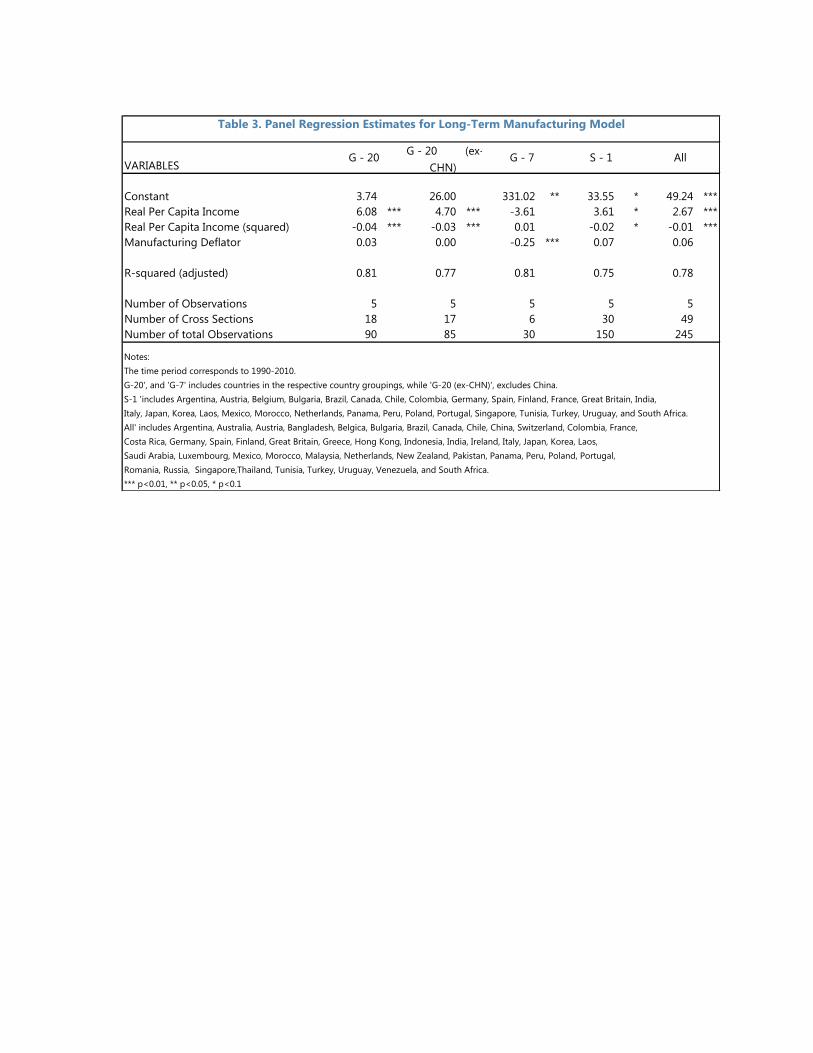
We run panel regressions to explore the association between the manufacturing-to-output

ratio (relative to that in the United States) with relative costs and real per-capita income

levels.. Concretely, we estimate the following specification:

MRt,i = α + β1YRt,i + β2YRSQt,i + β3PRt,i + µ, (2)

where MRt,i denotes the ratio of the share of manufacturing in output in country i to that of

the U.S. (both in nominal terms) at time t, YRt,i denotes the ratio of real per capita income in

country i to that of the U.S. at time t, YRSQt,i denotes the same variable but raised to the

square power, and PRt,i represents the manufacturing deflator (calculated on US$ values) in

country i to that of the U.S., at time t; the latter variable serves as a proxy for relative

currency appreciations. For robustness considerations, the regression in (2) was estimated for

20-year rolling periods (beginning in 1970), and for a number of alternative country

groupings including developed, emerging markets, and developing economies.

9

Results suggest that it is unlikely that the manufacturing-to-output ratio in emerging market

economies will lose significant ground vis-à-vis the U.S. in the next few years. The estimates

suggest that the share of manufacturing in output vis-à-vis the U.S. begins to decrease for

countries that reach real per capita incomes between 40 and 70 percent of those in the U.S.

(i.e., at about those levels of relative real per capita income the quadratic term in equation (2)

offsets the linear term). Since that level is rather distant from the 20 percent around which

emerging market countries are clustered now, a decline in the relative ratios due to per capita

income convergence seems unlikely in the medium term (though might occur in the longer

term). The effect of relative currency appreciations is less robust, but results for country

samples including developed and developing countries suggest a negative effect of up to

0.7 percentage points in the relative ratio of manufacturing to output for a 10 percent

currency appreciation; this effect is much stronger (and statistically significant) for G-7

countries (Table 3).9

Could U.S. manufacturing exports provide an outlet for stronger growth in the sector

during the coming years?

A look at the last few decades suggests that U.S. manufacturing exports have been more

resilient than total manufacturing production. While manufacturing has decreased as a share

of GDP, manufacturing exports have remained about constant, and have come to constitute a

larger share of total manufacturing output. However, in spite of this resilience, U.S.

manufacturing exports have lost market share during the past few decades, in particular with

respect to China and other emerging market economies. The application of a ‘Constant

Market Share’ analysis to U.S. manufacturing exports suggests that the loss in market share

is in part explained by the fact that U.S. exports have been primarily directed towards less

dynamic regions.10

These elements allow exploring a possible channel of contribution of manufacturing to

medium-term U.S. GDP growth. As indicated above, it is unlikely that convergence in per-

capita income during the next few years will be enough for the manufacturing-to-output ratio

in emerging market economies to begin losing ground vis-à-vis that in the U.S. However, this

does not mean that the manufacturing share in U.S. GDP will necessarily decrease.11

9 The source for the data is the United Nations Database. Results reported in Table 3 correspond to fixed-effect

regressions for 1990–2010. Details on the results for non-fixed effect regressions, other time periods, and other

country groupings, as well as databases, are available from the authors upon request.

10 The Constant Market Share Analysis is based on the idea that the product and geographical structure of a

country’s exports can affect is export growth. It constitutes a common method of analysis in international trade.

11 The model does not allow establishing to what extent changes in the relative ratio of manufacturing-to-output

between two countries will occur through changes in the numerator, the denominator or both. Evidence for the

past decade suggests that the U.S. manufacturing-to-output share, as well as the relative price of manufacturing,

have both stabilized. Calculations on the potential impact of manufacturing in GDP growth assume that the

(continued…)

10

Emerging market economies are projected to continue growing at faster rates than developed

economies and to increasingly contribute to global trade (including of manufacturing goods),

which will continue to grow faster than world GDP.12 If the U.S. share in G-20

manufacturing exports remains constant through the end of the decade at the level observed

in 2011, manufacturing could add up to 0.4 percentage points to growth per year through

2020. Further, an increase of 1 percentage point in the U.S. share in total G-20 manufacturing

exports by 2020 would result in an additional 0.2 percentage points of growth per year.

Moreover, the results from estimating (2) suggest that a one standard deviation increase in

currency appreciation (equivalent to a 25 percent increase in manufacturing prices in

comparator countries in US$ terms) through 2020 could add up to about 0.5 percentage

points of additional GDP growth in the United States per year. Contributions to growth of

such magnitudes are significant, given that manufacturing contributed less than

0.2 percentage points to growth per year (on average) during the last decade.13

For manufacturing to have a first-order impact on growth during the next few years, the U.S.

will have to diversify its export base. In order to keep its share in international markets, the

U.S. will have to diversify its manufacturing exports base to more dynamic regions

(e.g., Advanced and Emerging Asia). COMTRADE data compiled by the United Nations

suggest that the share of U.S. manufacturing exports to the world’s dynamic regions remains

low, but that has grown significantly during the past decade. In this connection, a look at the

product composition of exports suggests that the external sales of chemical and plastic

materials (all of which use energy intensively) have broadly outperformed the external sales

of other sectors during the past decade. The growth rate of exports of machinery (electrical

ant other), and transport equipment (which together account to about 40 percent of exports),

has been less impressive, but the lower-than-average growth rates masks a change in the

direction of exports, with sales to more dynamic regions (most notably Emerging Asia)

increasing, and those to more mature markets stabilizing or decreasing during the past few

years. The more attractive input costs vis-à-vis other G-7 economies (as pointed out in

Section III) also bodes well for the future performance of U.S. exports.

VI. CONCLUDING THOUGHTS

While overly optimistic claims of a U.S. manufacturing renaissance seem unwarranted, some

sectors have indeed rebounded strongly following the Great Recession. Available data

suggests that there are sectors within the durable goods category that have withstood the

relative price of manufacturing remains stable vis-à-vis GDP deflator. Moreover, it is assumed that the share of

manufacturing exports in total manufacturing remains unchanged.

12 Growth and trade projections used in the analysis are those in World Economic Outlook (2013).

13 Manufacturing contributed about 0.7 percentage points (pp) per year to growth in the 1970s, and about 0.5 pp

in the 1980s and the 1990s. The contribution to growth was larger in the 1960s (about 1.3 pp/year) and the

1950s (1.1 pp/year), on average.

11

Great Recession well or have rebounded strongly thereafter, possibly foreshadowing a strong

manufacturing presence in the U.S. and the global marketplace in some subsectors.

A number of ongoing factors are likely to positively impact the profitability of the U.S.

manufacturing sector in the near-to-medium term. First, a combination of declining

production costs—falling natural gas prices and ULC, and some real depreciation of the U.S.

dollar—could catalyze new investment in the manufacturing sector, providing a boost to

growth. Second, expanding shale oil and gas activity will create new demand for U.S.

manufacturing output going forward.

The contribution of manufacturing exports to growth could exceed those of the recent past,

fueled by rising global trade. U.S. manufacturing exports have proven resilient during the

crisis. Further increases will require that the U.S. diversify further its export base towards the

more dynamic world regions. In the long term, it is likely that a U.S. REER depreciation and

the convergence of real per capita income in fast growing emerging market economies would

result in a gradual increase in the manufacturing-to-output ratio in the U.S. vis-à-vis such

economies.

12

References

The Atlantic, 2012, http://www.theatlantic.com/magazine/archive/2012/12/the-insourcing-

boom/309166/?single_page=true (November).

Citibank, 2012, “Is a Renaissance in U.S. Manufacturing Forthcoming?” Citi Research (May

31).

U.S. Energy Information Agency, 2013, “Annual Energy Outlook, 2013,” Washington D.C.

Financial Times, 2012, http://www.ft.com/intl/cms/s/0/65230da8-0317-11e2-a484-

00144feabdc0.html#axzz2EnpQZY00 (September 21).

Goldman Sachs, 2013, “The US Manufacturing Renaissance: Fact or Fiction?”

U.S. Economic Analyst, Issue No: 13/12 (March 22).

Herrendorf B., R. Rogerson, and A. Valentinyi, forthcoming, “Growth and Structural

Transformation,” Handbook of Economic Growth.

Helper, S., T. Krueger and H. Wial, 2012, “Why Does Manufacturing Matter? Which

Manufacturing Matters? A Policy Framework,” Metropolitan Policy Program,

Brookings Institution, February, Washington D.C.

Houseman S., C. Kurz, P. Lengermann, and B. Mandel, 2011, “Offshoring Bias in U.S.

Manufacturing,” Journal of Economic Perspectives 25, 111–132.

International Monetary Fund, 2013, “World Economic Outlook,” (April).

McKinsey Global Institute, 2012, “Manufacturing the Future: The Next Era of Global

Growth and Innovation” (November).

Morgan Stanley, 2013, “US Manufacturing Renaissance Is It a Masterpiece or a (Head)

Fake?” (April 29).

New York Times, 2012, http://www.nytimes.com/2012/11/25/magazine/skills-dont-pay-the-

bills.html?ref=itstheeconomy (November 25, 2012).

White House, State of the Union Address, 2013, http://www.whitehouse.gov/the-press-

office/2013/02/12/remarks-president-state-union-address (February 12).

13

10

12

14

16

18

20

22

1980 1984 1988 1992 1996 2000 2004 2008 2012

Manufacturing vs. Services

(Percent of GDP)

Manufacturing

Services (Finance, Insurance, Real Estate, Leasing)

0

5

10

15

20

25

30

35

40

2000 2001 2002 2003 2004 2005 2006 2007 2008 2009 2010 2011 2012

Manufacturing Sector by Country 1/

(Percent of Total World Manfuacturing)

USA China EU Germany

Figure 1. Historical Look at the U.S.

Manufacturing Sector

Source: Haver Analytics and World Bank Development Indicators.

1/ Values for 2011 and 2012 are staff estimates based on IP growth rates of

each country.

14

Figure 2. Durable and Nondurable Goods

90

95

100

105

110

115

120

125

130

135

140

2006Q1 2007Q1 2008Q1 2009Q1 2010Q1 2011Q1 2012Q1 2013Q1

Manufacturing Production and GDP 2006 - 2013

( Index, 2009Q2 = 100)

Real GDP

Manufacturing IP

70

75

80

85

90

95

100

105

110

2003Q1 2005Q1 2007Q1 2009Q1 2011Q1 2013Q1

U.S. Manufacturing, Durable vs. Nondurable Goods

(Index, 2007 = 100)

Durables

Nondurables

Source: Haver Analytics.

15

Figure 3. Comparison of Rebounds

Across Recessions

90

95

100

105

110

115

120

125

130

135

140t-

10

t-9

t-8

t-7

t-6

t-5

t-4

t-3

t-2

t-1 t

t+1

t+2

t+3

t+4

t+5

t+6

t+7

t+8

t+9

t+1

0

t+1

1

t+1

2

t+1

3

t+1

4

t+1

5

Durable Goods Manufacturing - IP

Jul 1990 - Mar 1991 Mar - Nov 2001 Dec 2007 - Jun 2009

90

95

100

105

110

115

120

t-1

0

t-9

t-8

t-7

t-6

t-5

t-4

t-3

t-2

t-1 t

t+1

t+2

t+3

t+4

t+5

t+6

t+7

t+8

t+9

t+1

0

t+1

1

t+1

2

t+1

3

t+1

4

t+1

5

Nondurable Manufacturing - IP

Jul 1990 - Mar 1991 Mar - Nov 2001

Dec 2007 - Jun 2009

Source: Haver Analytics.

1/ For the Dec 07 - Jun 09 recession, t+15 represents January 2013.

16

Figure 4. Components of Durable

and Nondurable Goods

70

75

80

85

90

95

100

105

110

2007Q1 2008Q1 2009Q1 2010Q1 2011Q1 2012Q1 2013Q1

U.S. Manufacturing, Components of Nondurables

(Index, 2007 = 100)

Chemicals

Petroleum Products

Plastics and Rubbers

40

50

60

70

80

90

100

110

120

130

140

2007Q1 2008Q1 2009Q1 2010Q1 2011Q1 2012Q1 2013Q1

U.S. Manufacturing, Components of Durables

(Index, 2007 = 100)

Machinery

Motor Vehicles

Computers and Electronics

Source: Haver Analytics.

17

Figure 5. Manufacturing Rebound in G-7 Countries

65

70

75

80

85

90

95

100

105

110

115

Jan-06 Jan-07 Jan-08 Jan-09 Jan-10 Jan-11 Jan-12 Jan-13

Manufacturing - Industrial Production

(Indices, Avg 2007 = 100)

US

GER

FRA

ITL

JPN

UK

CAN

40

50

60

70

80

90

100

110

120

Jan-06 Jan-07 Jan-08 Jan-09 Jan-10 Jan-11 Jan-12 Jan-13

Durable Goods Manufacturing - Industrial Production

(Indices, Avg 2007 = 100)

US

GER

FRA

ITL

JPN

UK

CAN

Source: Haver Analytics.

18

Figure 6. Manufacturing Production in Selected Countries

75

80

85

90

95

100

105

ITL JPN FRA CAN US UK GER

Manufacturing: June 2011

(Indices, Avg 2007 = 100)

75

80

85

90

95

100

105

ITL FRA JPN CAN UK US GER

Manufacturing: April 2013

(Indices, Avg 2007 = 100)

-1.0

-0.6

-0.2

0.2

0.6

1.0

1.4

JPN GER MEX CHN UK ITA FRA CAN

Correlation with Growth in US

Manufacturing

(2007-June 2011)

-0.6

-0.4

-0.2

0.0

0.2

0.4

0.6

0.8

1.0

ITA FRA CHN GER UK CAN JPN MEX

Correlation with Growth in US

Manufacturing

(July 2011-February 2013)

70

75

80

85

90

95

100

JPN ITL FRA CAN GER UK US

Durable Goods Manufacturing: June 2011

(Indices, Avg 2007 = 100)

60

70

80

90

100

110

ITL JPN UK FRA CAN GER US

Durable Goods Manufacturing: April 2013

(Indices, Avg 2007 = 100)

70

80

90

100

110

US CAN ITL FRA UK GER JPN

Nondurable Goods Manufacturing: July

2011

(Indices, Avg 2007 = 100)

70

80

90

100

110

ITL US CAN UK GER FRA JPN

Nondurable Goods Manufacturing: April

2013

(Indices, Avg 2007 = 100)

Source: Haver Analytics.

19

Figure 7. Natural Gas Production and Prices

0

2

4

6

8

10

12

14

16

18

0

500

1000

1500

2000

2500

3000

Jan-04 Jan-06 Jan-08 Jan-10 Jan-12

U.S. Natural Gas Production and Spot Price

(Billions of cubic feet, $/mmbtu)

Non-Shale Prod

Shale Prod

Total Prod

HH Spot Price (RHS)

0

50

100

150

200

250

300

Mar-97 Mar-01 Mar-05 Mar-09 Mar-13

Selected Natural Gas Spot Prices

(Index, 2005 = 100)

Indonesian Liq Gas

Henry Hub

Russian Border

Source: U.S. Energy Information Agency.

20

(1) (2) (3) (4) (5)

VARIABLES Spread REER ULC Spread-REER All

Spread 0.000774** 0.000780** -0.000225

(0.0466) (0.0341) (0.653)

lnd(REER) -0.170*** -0.170*** -0.143***

(1.23e-07) (9.87e-08) (7.41e-06)

lnd(UCL) -0.418*** -0.352***

(1.59e-10) (4.50e-08)

Constant -0.0240*** -0.0247*** 0.0269*** -0.0253*** -0.0156*

(0.00324) (0.00152) (0.00328) (0.00108) (0.0754)

Observations 303 303 260 303 260

R-squared 0.708 0.735 0.778 0.740 0.798

Number of Countries 7 7 7 7 7

Table 1. Panel Regression Estimates for Total Manufacturing Production

Dependent variable is the log difference of IP manufacturing. Spread is the gas price spread between the rest of G-7 countries and U.S. ;

lnd(REER) is the log difference of the real effective exchange rate; lnd(ULC) is the log difference of unit labor cost. p-value in parentheses. All

regressions include a lag of log difference of IP manufacturing, and a Global Crisis time dummy in addition to quarterly time fixed effects. ***

p<0.01, ** p<0.05, * p<0.1.

Table 2. Panel Regression Estimates for Durable and Nondurable Manufacturing Production

(1a) (1b) (2a) (2b) (3a) (3b) (4a) (4b) (5a) (5b)

D Goods Non D Goods D Goods Non D Goods D Goods Non D Goods D Goods Non D Goods D Goods Non D Goods

VARIABLES Spread Spread REER REER ULC ULC Spread & REER Spread & REER ALL ALL

Spread 0.000627 -0.0000863 0.000634 -0.0000834 -0.0017 -0.000731*

(0.477) (0.759) (0.465) (0.766) (0.152) (0.073)

ln(REER) -0.223*** -0.0483** -0.224*** -0.0482*** -0.227*** -0.463*

-0.00247 -0.42 -0.00248 -0.0425 -0.00235 -0.0679

ln(ULC) -0.439*** -0.0648 -0.357** -0.0553

-0.00235 -0.181 -0.0148 -0.268

Constant 0.00313 0.00471 0.000789 0.0036 0.0899*** 0.00204 0.000213 0.00372 -0.0609*** 0.0097

(0.886) (0.487) (0.971) (0.592) (-3.11E-05) (0.774) (0.992) (0.581) (0.004) (0.172)

Observations 303 303 303 303 260 260 303 303 260 260

R-Squared 0.409 0.319 0.429 0.33 0.499 0.333 0.43 0.33 0.525 0.353

Number of Countries 7 7 7 7 7 7 7 7 7 7

The dependent variable is the log difference of IP durable (a) and non-durable (b) manfucaturing. Spread is the gas price spread between the rest of the G-7 countries and the U.S.;

ln(REER) is the log difference of the real effective exchange rate; ln(ULC) is the log differece of unit labor cost. All regressions include a lag of log difference of IP (durable and

non-durable, accordingly) manufacturing, and a Global Crisis time dummy in addition to quarterly time fixed effects. *** p<0.01, **p<0.05, *p<0.a.

VARIABLES

Constant 3.74 26.00 331.02 ** 33.55 * 49.24 ***

Real Per Capita Income 6.08 *** 4.70 *** -3.61 3.61 * 2.67 ***

Real Per Capita Income (squared) -0.04 *** -0.03 *** 0.01 -0.02 * -0.01 ***

Manufacturing Deflator 0.03 0.00 -0.25 *** 0.07 0.06

R-squared (adjusted) 0.81 0.77 0.81 0.75 0.78

Number of Observations 5 5 5 5 5

Number of Cross Sections 18 17 6 30 49

Number of total Observations 90 85 30 150 245

Notes:

The time period corresponds to 1990-2010.

G-20', and 'G-7' includes countries in the respective country groupings, while 'G-20 (ex-CHN)', excludes China.

S-1 'includes Argentina, Austria, Belgium, Bulgaria, Brazil, Canada, Chile, Colombia, Germany, Spain, Finland, France, Great Britain, India,

Italy, Japan, Korea, Laos, Mexico, Morocco, Netherlands, Panama, Peru, Poland, Portugal, Singapore, Tunisia, Turkey, Uruguay, and South Africa.

All' includes Argentina, Australia, Austria, Bangladesh, Belgica, Bulgaria, Brazil, Canada, Chile, China, Switzerland, Colombia, France,

Costa Rica, Germany, Spain, Finland, Great Britain, Greece, Hong Kong, Indonesia, India, Ireland, Italy, Japan, Korea, Laos,

Saudi Arabia, Luxembourg, Mexico, Morocco, Malaysia, Netherlands, New Zealand, Pakistan, Panama, Peru, Poland, Portugal,

Romania, Russia, Singapore,Thailand, Tunisia, Turkey, Uruguay, Venezuela, and South Africa.

*** p<0.01, ** p<0.05, * p<0.1

All

Table 3. Panel Regression Estimates for Long-Term Manufacturing Model

G - 20G - 20 (ex-

CHN)G - 7 S - 1