Terrestrial Surface Energy Balance 1. Introduction Solar radiation and atmospheric longwave

THE UNIVERSITY OF READING
Department of Meteorology
The energy balance of urban areas
Ian Nicholas Harman
A thesis submitted for the degree of Doctor of Philosophy
October 2003

Declaration
I confirm that this is my own work and the use of all material from other
sources has been properly and fully acknowledged.
Ian Nicholas Harman
ABSTRACT
Urban areas have different climatologies to their rural surroundings. The physical mechanisms
responsible for these differences are not accurately known. This work contributes to the better
understanding of the physical processes acting in urban areas.
The role of surface morphology in determining the surface energy balance of an urban area and
the subsequent impacts on the planetary boundary layer are investigated. The urban street canyon
is used as the generic unit of the urban surface in a range of analytic, experimental and numerical
investigations.
The first part of this work considers the role of surface morphology on the individual terms of the
surface energy balance. An analytical approach was used to investigate the exchange of diffuse
radiation in a street canyon. Multiple reflections of radiation were found to play an important role.
An experimental approach and process based modelling were used to analyse the turbulent flux of
a scalar from a street canyon. The variation of the flow and turbulence with surface morphology
both above and within the street canyon was found to determine the surface flux densities. The
competing effects of surface geometry, which decreases theflux densities, and the increased sur-
face area, which increases the total fluxes, determines the net effect of surface morphology on the
energy balance.
The second part of the work considers the interaction between the surface energy balance and the
boundary layer. A coupled model of the surface energy balance and boundary layer was used
to investigate the impact of surface morphology on the boundary layer. The impacts of surface
morphology, on their own, result in realistic surface, canopy and boundary layer urban heat islands.
An investigation into simplifying the urban street canyon energy balance shows that two surfaces,
a roof surface and a canyon surface, are needed to represent the surface energy balance of urban
areas. The adjustment of the boundary layer under advectionfrom a rural to an urban area is
suggested to be a key process even at low wind speeds.

Acknowledgements
I express my thanks to my supervisors, Dr. S. E. Belcher and M.J. Best, for their invaluable sup-
port, assistance and guidance throughout this project. I amgrateful for the support and guidance
given by Prof. K. Browning and Prof. P. Valdes in their direction of this work.
Thanks also go to Dr. J. F. Barlow in formulating and buildingthe experiments and for valuable
discussions in interpreting the results. I acknowledge thetechnical support of the experiments by
S. Gill and A. Lomas. I thank P. Clark for graciously steppingin to support the project when
unforeseen circumstances occured in the later stages. Thanks must also go the Boundary-Layer
group and my fellow PhD students for the support and guidancein the presentation of this work and
the wider support given. Thanks go to J. Finnigan and to Prof.K. Shine for their input concerning
the work in Chapter 2.
I am immensely grateful to my family for their unwaivering support and encouragement over the
years. I am also grateful to all my friends, especially Chloe, James and Sheula, Baz, Litka and
Ulash, within and outside the department for being there andhelping me to keep perspective.
Many thanks to all at the Department of Meteorology for making the department such a friendly
place where it is a pleasure to work. Finally, thanks to the members of the University of Reading
Mixed Hockey Club and my fellow squash players in helping me forget things when I needed to.
This research was funded by the Natural Environment Research Council and the Met Office
through a CASE award.

Contents
Abstract i
Acknowledgements ii
Table of contents iii
Glossary of terms vii
1 Introduction 1
1.1 Scale and the urban surface . . . . . . . . . . . . . . . . . . . . . . . . .. . . . 3
1.2 The urban boundary layer . . . . . . . . . . . . . . . . . . . . . . . . . . .. . . 5
1.2.1 The inertial sub-layer . . . . . . . . . . . . . . . . . . . . . . . . . .. . 7
1.2.2 The roughness sub-layer and canopy layer . . . . . . . . . . .. . . . . . 8
1.3 The urban energy balance . . . . . . . . . . . . . . . . . . . . . . . . . . .. . . 11
2 Radiative exchange in an urban street canyon 18
2.1 Introduction . . . . . . . . . . . . . . . . . . . . . . . . . . . . . . . . . . . .. 18
2.2 Methodology . . . . . . . . . . . . . . . . . . . . . . . . . . . . . . . . . . . . 20
2.3 Exchange of diffuse radiation . . . . . . . . . . . . . . . . . . . . . .. . . . . . 21
2.3.1 Fundamentals of radiative exchange . . . . . . . . . . . . . . .. . . . . 21
2.3.2 Shape factors for an urban canyon . . . . . . . . . . . . . . . . . .. . . 22
2.3.3 Exact solution . . . . . . . . . . . . . . . . . . . . . . . . . . . . . . . 24
2.3.4 Approximate solutions . . . . . . . . . . . . . . . . . . . . . . . . . .. 25
2.3.5 Application to the urban street canyon . . . . . . . . . . . . .. . . . . . 25
iii

iv
2.4 Comparison of the exact solution with the approximations . . . . . . . . . . . . 26
2.4.1 Exact solution - longwave radiation . . . . . . . . . . . . . . .. . . . . 26
2.4.2 Approximate methods - longwave radiation . . . . . . . . . .. . . . . . 28
2.4.3 Errors of the approximate solutions . . . . . . . . . . . . . . .. . . . . 30
2.4.4 Shortwave radiation . . . . . . . . . . . . . . . . . . . . . . . . . . . .32
2.5 Summary and conclusions . . . . . . . . . . . . . . . . . . . . . . . . . . .. . 35
3 Turbulent exchange in an urban street canyon 37
3.1 Introduction . . . . . . . . . . . . . . . . . . . . . . . . . . . . . . . . . . . .. 37
3.2 The bulk aerodynamic formulation for surface fluxes . . . .. . . . . . . . . . . 39
3.3 The naphthalene sublimation technique for scalar fluxes. . . . . . . . . . . . . . 41
3.4 Flow patterns in an urban street canyon . . . . . . . . . . . . . . .. . . . . . . 43
3.5 Resistance network for an urban street canyon . . . . . . . . .. . . . . . . . . . 46
3.5.1 Wind profile in the inertial sub-layer . . . . . . . . . . . . . .. . . . . . 48
3.5.2 Transport from the roof . . . . . . . . . . . . . . . . . . . . . . . . . .. 51
3.5.3 Transport from the recirculation region . . . . . . . . . . .. . . . . . . 51
3.5.4 Transport from the ventilated region . . . . . . . . . . . . . .. . . . . . 53
3.5.5 Model parameters . . . . . . . . . . . . . . . . . . . . . . . . . . . . . . 55
3.6 Comparison with observations . . . . . . . . . . . . . . . . . . . . . .. . . . . 55
3.6.1 Flux off the roof . . . . . . . . . . . . . . . . . . . . . . . . . . . . . . 55
3.6.2 Flux off the street . . . . . . . . . . . . . . . . . . . . . . . . . . . . . .56
3.6.3 Flux off the walls . . . . . . . . . . . . . . . . . . . . . . . . . . . . . . 57
3.6.4 Total flux . . . . . . . . . . . . . . . . . . . . . . . . . . . . . . . . . . 58
3.7 Roughness lengths for scalars . . . . . . . . . . . . . . . . . . . . . .. . . . . . 61
3.8 Sensitivity to surface morphology . . . . . . . . . . . . . . . . . .. . . . . . . 63
3.9 Summary and conclusions . . . . . . . . . . . . . . . . . . . . . . . . . . .. . 64
4 Energy balance and boundary layer interactions 67
4.1 The surface energy balance model . . . . . . . . . . . . . . . . . . . .. . . . . 69

v
4.1.1 The thin-layer approximation . . . . . . . . . . . . . . . . . . . .. . . 69
4.1.2 The substrate temperature profile . . . . . . . . . . . . . . . . .. . . . . 71
4.1.3 The radiative and turbulent fluxes . . . . . . . . . . . . . . . . .. . . . 72
4.2 The energy balance for an urban street canyon . . . . . . . . . .. . . . . . . . . 73
4.2.1 Interaction terms - Radiative fluxes . . . . . . . . . . . . . . .. . . . . 74
4.2.2 Interaction terms - Turbulent fluxes . . . . . . . . . . . . . . .. . . . . 76
4.3 Boundary layer formulation . . . . . . . . . . . . . . . . . . . . . . . .. . . . . 77
4.4 The role of surface area . . . . . . . . . . . . . . . . . . . . . . . . . . . .. . . 79
4.5 Case study . . . . . . . . . . . . . . . . . . . . . . . . . . . . . . . . . . . . . . 81
4.5.1 Case study: The bulk energy balances . . . . . . . . . . . . . . .. . . . 84
4.5.2 Case study: The facet energy balances . . . . . . . . . . . . . .. . . . . 86
4.5.3 Case study: Surface and boundary-layer temperatures. . . . . . . . . . . 88
4.5.4 Case study: Summary . . . . . . . . . . . . . . . . . . . . . . . . . . . 92
4.6 The effects of incomplete treatment radiation . . . . . . . .. . . . . . . . . . . 93
4.7 Sensitivity to urban morphology . . . . . . . . . . . . . . . . . . . .. . . . . . 94
4.7.1 Sensitivity to the canyon aspect ratio . . . . . . . . . . . . .. . . . . . . 95
4.7.2 Sensitivity to the planar area index . . . . . . . . . . . . . . .. . . . . . 96
4.7.3 Co-varying the canyon aspect ratio and planar area index . . . . . . . . . 97
4.7.4 Sensitivity to canyon orientation . . . . . . . . . . . . . . . .. . . . . . 98
4.7.5 Sensitivity to urban morphology: Summary . . . . . . . . . .. . . . . . 99
4.8 Summary and conclusions . . . . . . . . . . . . . . . . . . . . . . . . . . .. . 100
5 A simplified urban energy balance 102
5.1 Intoduction . . . . . . . . . . . . . . . . . . . . . . . . . . . . . . . . . . . . .102
5.2 Approximations to the urban street canyon model . . . . . . .. . . . . . . . . . 104
5.3 Comparison between theF1, F2 andF4 schemes . . . . . . . . . . . . . . . . . 107
5.4 Summary and conclusions . . . . . . . . . . . . . . . . . . . . . . . . . . .. . 112
6 Adjustment of the boundary layer over urban areas 114

vi
6.1 Introduction . . . . . . . . . . . . . . . . . . . . . . . . . . . . . . . . . . . .. 114
6.2 Representation of advection in a one-dimensional setting . . . . . . . . . . . . . 117
6.3 Impacts of advection . . . . . . . . . . . . . . . . . . . . . . . . . . . . . .. . 119
6.3.1 Diurnal cycle of temperatures . . . . . . . . . . . . . . . . . . . .. . . 119
6.3.2 Diurnal cycle of the energy balance . . . . . . . . . . . . . . . .. . . . 120
6.3.3 Adjustment with fetch . . . . . . . . . . . . . . . . . . . . . . . . . . .121
6.4 Summary and implications . . . . . . . . . . . . . . . . . . . . . . . . . .. . . 124
7 Conclusions 126
7.1 Summary of thesis . . . . . . . . . . . . . . . . . . . . . . . . . . . . . . . . .126
7.2 Conclusions . . . . . . . . . . . . . . . . . . . . . . . . . . . . . . . . . . . . .128
7.3 Impact on the wider picture . . . . . . . . . . . . . . . . . . . . . . . . .. . . . 132
7.4 Future work . . . . . . . . . . . . . . . . . . . . . . . . . . . . . . . . . . . . . 133
A Solar radiation in an urban street canyon 135
B Turbulence closure in the boundary layer 144
References 148
vii
Glossary of terms
The individual terms are introduced in detail within the main text.
Standard termst time (s)
(x, y, z) standard orthogonal co-ordinate system either aligned east-west, north-south orx
aligned with the mean wind.
ρ density of air (1.2 kg m−3)
g acceleration due to gravity (9.8 m s−2)
cp specific heat capacity of air at constant pressure (1004 J kg−1K−1)
θs(Ti) surface temperature (of surfacei) (K)
δij Kronecker-delta operator.
Averaging operators
x time-average of propertyx
〈x〉 spatial-average of propertyx
x′ instantaneous deviation ofx from its time- and spatial- average
x∗ scaling value forx′
Surface dimensionshe height of the buildings (m)
we width of the street (m)
re width of the generic surface unit (m)
λp planar area index
λf frontal area index
z2 reference height in the inertial sub-layer (m)
zi height of the boundary layer (m)

viii
Subscripts
i, j, k general subscripts
rf roof
s surface
st street
us (ds) upstream (downstream) section of the street (Chapter 3)
wl (w1, w2) wall
uw (dw) upstream (downstream) wall (Chapter 3)
c canyon
sk sky
Boundary layer variables
v(z) vertical profile of the horizontal wind vector aligned in thex−y directions (m s−1)(
= (u(z), v(z)))
U(z) vertical profile of the wind speed (m s−1)
Uδ wind speed at the top of the inertial sub-layer (m s−1)
(ug, vg) geostrophic wind vector (m s−1)
(uF, v
F) mean wind for the upstream profile (Chapter 6) (m s−1)
τ turbulent stress (kg m−1s−2)
u∗ surface friction velocity (m s−1)
λ (λe) (equilibrium) mixing length (m)
θ(z) vertical profile of potential temperature (K)
L Monin-Obukhov length (m)
Ri Richardson number
Ψm,Ψh integrated stability functions for momentum and heat respectively
θF
mean potential temperature for the upstream profile (K)
LF
distance from the change in surface type (fetch) (Chapter 6)(m)
Km,Kh turbulent diffusivities for momentum and heat respectively (m2s−1)
H surface sensible heat flux (W m−2)
w∗ scaling for the vertical velocity (m s−1)
ix
Energy balance variables
K↓ total downwelling wavelength-integrated solar radiativeflux density (W m−2)
K↑ total upwelling wavelength-integrated solar radiative flux density (W m−2)
L↓ downwelling wavelength-integrated longwave radiative flux density (W m−2)
L↑ upwelling wavelength-integrated longwave radiative flux density (W m−2)
Q∗ net radiative flux density (W m−2)
Ksf (Kdf ) direct (diffuse) component of the solar radiative flux density (W m−2)
H sensible heat flux density (W m−2)
LE latent heat flux density (W m−2)
G ground heat flux density (W m−2)
k thermal conductivity of the substrate (W k−1m−1)
cs volumetric heat capacity of the substrate (J K−1m−3)
αi wavelength-integrated albedo for the material of surfacei
εi wavelength-integrated emissivity for the material of surfacei
TL
linearising temperature (273 K)
Tin substrate interior temperature (K)
Gin interior ground heat flux (W m−2)
wT
transport velocity for the turbulent fluxes (m s−1)
F1,F2,F4 approximations to the full canyon energy balance (Chapter 5)
Radiation variables (Chapter 2)
Λi(j) flux density of incoming diffuse radiation onto surfacei which has originated
directly from surfacej (W m−2)
Λi total flux density of incoming diffuse radiation onto surface i (W m−2)
Ωi flux density of emitted diffuse radiation from surfacei (W m−2)
Bi total flux density of diffuse radiation away from surfacei (W m−2)
Qi net radiative flux density for surfacei (W m−2)
Fij matrix of shape factors
Γij matrix for radiative interaction
ψij inverse ofΓij
R0,R1 approximation methods to full solution for radiative exchange
x
Turbulent transport variables (Chapter 3)
X generic scalar
z0m , z0X
roughness lengths for momentum andX, respectively, pertaining to the surface
material (m)
z0T , zXT roughness lengths for momentum andX, respectively, pertaining to the entire
canyon unit (m)
dT
displacement height pertaining to the entire canyon unit (m)
rX resistance to the turbulent transport of scalarX (s m−1) - often relates to the
transport across an internal boundary layer
r∆X
resistance to the turbulent transport of scalarX across a free shear layer (s m−1)
wX turbulent transport velocity for the flux density of scalarX (m s−1)
wi turbulent transport velocity for the flux density from surfacei (m s−1)
wc turbulent transport velocity for the flux density out of the canyon cavity (m s−1)
wt turbulent transport velocity for the total flux density fromthe (canyon) surface
into the boundary layer (m s−1)
w0t turbulent transport velocity for the flux density from a flat surface of equivalent
surface material (m s−1)
Lr maximum length of the recirculation zone (m)
Lse length of the sloping edge of the recirculation zone (m)
ui wind speed representative of the turbulent transport from surfacei (m s−1)
uct wind speed representative of turbulent transport at canyontop (m s−1)
δi depth of the internal boundary layer formed along surfacei (m)
α1, α2 coefficients for the deceleration of the flow in the canyon cavity.
cD
turbulent drag coefficient (kg m−3)
CD
turbulent drag coefficient based on the wind speed at building height (kg m−3)

CHAPTER ONE
Introduction
The lowest layers of the atmosphere are known as theplanetary boundary layeror simply the
boundary layer. Stull (1988) defines the boundary layer as “that part of the atmosphere that is
directly influenced by the presence of the Earth’s surface, and responds to surface forcings with
a time scale of about an hour or less.” Boundary layer meteorology, the study of this layer of the
atmosphere, is characterised by the study of the turbulent nature of the boundary layer.
The airflow and thermal structure of the boundary layer is determined by the Earth’s surface. In
particular, thesurface energy balance, the partitioning of energy at the surface into different forms,
and the drag exerted by the surface determine the surface temperature and the vertical profiles of
wind and temperature in the boundary layer. Urban areas alter the material and aerodynamic
character of the surface, greatly affecting the surface energy balance as well as the dynamic and
thermodynamic nature of the boundary layer. These modifications to the local climate are the core
topics ofurban meteorologyandurban climatology.
Urban modifications to the local climate are manifested in a variety of forms. Urban areas are
generally warmer, less windy and drier in a relative sense than their rural surroundings (e.g. Oke,
1987). However, the role of the rural surroundings in determining these modifications cannot be
understated (Arnfield, 2003). The most prominent feature ofthe local climate of urban areas is the
well knownurban heat island. This is a transient feature of urban areas, usually nocturnal, where
the urban surface and near-surface air temperatures are warmer than their rural surroundings. Oke
(1982) presents a number of physically based explanations for the urban heat island. The precise
causality is different for each urban area with the reduction in moisture availability, changes in
the surface material properties and reduced longwave radiative cooling through radiative trapping
considered to be the dominant processes (Oke, 1987; Okeet al., 1991; Arnfield, 2003).
1

CHAPTER 1: The surface energy balance and boundary layer 2
Investigation of the thermal and dynamic properties of urban areas is important in a range of
applications. Heat stress resulting from the urban heat island can be a major concern for public
health (e.g. Dabbertet al., 2000). Similarly the dispersion characteristics of pollutants, known to
depend on the location of the source (Oke, 1987) and synopticconditions (Ketzelet al., 2002),
have important impacts on public health. More recently attention has focussed on the dispersal of
hazardous chemical or biological releases within urban areas. Architects and building engineers
require detailed knowledge of the airflow in urban areas to determine the structural strength and
energy requirements of new buildings. Finally, the increasing resolution of numerical weather
prediction models makes the practical forecasting of the weather within urban areas a real possi-
bility. Such work will also allow the assessment of whether urban areas impact significantly upon
mesoscale weather systems as has been speculated (e.g. Bornstein and Thompson, 1981; Born-
stein and Lin, 2000; Rozoff and Adegoke, 2003). Accurate, but simple, methods to incorporate
the range of dynamic and thermodynamic influences on the boundary layer across the full range
of urban types and synoptic conditions are therefore required.
A range of methods have been used to investigate the urban boundary layer and urban energy
balance. These include wind and water tunnel simulations (e.g. Barlow and Belcher, 2002; Lu
et al., 1997a,b), numerical simulations (e.g. Hunteret al., 1992; Johnson and Hunter, 1995; Baik
and Kim, 1999; Liu and Barth, 2002), field experiments (e.g. Cleugh and Oke, 1986; Grimmond,
1992) and high resolution remote sensing (e.g. Lee, 1993).
This study focusses on one aspect of urban areas, namely the surface morphology, and how
it controls urban meteorology. Changes in the surface morphology are possibly the one property
common to all urban areas. It is therefore important to consider fully the impact of surface mor-
phology on all parts of the surface energy balance and boundary layer. The remainder of this
introductory chapter presents a brief overview of the energy balance and boundary layer of ur-
ban areas concentrating on the current understanding, the fundamental paradigms, concepts and
assumptions used throughout the thesis, as well as perceived gaps in knowledge. The specific
aims of this work are then introduced together with a more detailed outline of the thesis. Detailed
motivation for each of the sections of work are included at the beginning of those sections.

CHAPTER 1: The surface energy balance and boundary layer 3
1.1 Scale and the urban surface
The complex morphology of an urban area results in a range of effects in the boundary layer and
energy balance. The urban surface is notably highly non-homogeneous varying on a range of
spatial scales. Fundamental to understanding the physicalmechanisms responsible for the urban
modifications to the local climate is the spatial scale upon which the physical processes act. Figure
1.1 relates several topics within urban climatology to the typical spatial scales on which they are
considered (e.g. Britter and Hanna, 2003). Of course, physical processes acting on one spatial
scale can be influenced by others acting on a different spatial scale. For example the detailed
transport processes at the street scale determine the boundary conditions for the boundary layer
which in turn impacts larger scale processes. Similarly, the synoptic and regional scale forcing can
influence all of the smaller scales. A key aspect of urban meteorology concerns the description
and classification of the surface on the relevant spatial scale.
scaleNeighbourhood
scaleStreet
scaleCity
scaleRegional
100’s m 10,000’s m1000’s m
Pollution dispersion
Building design
Urban energy balance
Urban heat island
Impacts on the weather?
Figure 1.1: Schematic relating topics within urban climatology and their spatial scales.
Buildings impose two properties of the urban surface. Firstly, the total surface area is increased
from that of a planar surface. Secondly, the surface is deformed to accommodate the increase in
surface area. The termsurface geometryis used in this thesis specifically to denote the deformation
of the surface, i.e. the dimensions and separation of the buildings. The termsurface morphology
is used to denote the combined effects of increasing the surface area and the deformation of the
surface.
The full detail of the urban surface is only needed, and indeed only practical, for highly specific
studies, for instance into the dispersion of pollutants from a specific source within a building
array. More common is a requirement to classify the average effects of the urban surface on
the appropriate spatial scale. The simplest general methodto classify the surface morphological
CHAPTER 1: The surface energy balance and boundary layer 4
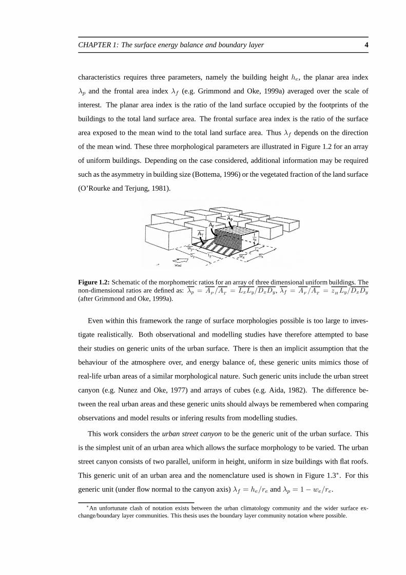
characteristics requires three parameters, namely the building heighthe, the planar area index
λp and the frontal area indexλf (e.g. Grimmond and Oke, 1999a) averaged over the scale of
interest. The planar area index is the ratio of the land surface occupied by the footprints of the
buildings to the total land surface area. The frontal surface area index is the ratio of the surface
area exposed to the mean wind to the total land surface area. Thusλf depends on the direction
of the mean wind. These three morphological parameters are illustrated in Figure 1.2 for an array
of uniform buildings. Depending on the case considered, additional information may be required
such as the asymmetry in building size (Bottema, 1996) or thevegetated fraction of the land surface
(O’Rourke and Terjung, 1981).
Figure 1.2: Schematic of the morphometric ratios for an array of three dimensional uniform buildings. Thenon-dimensional ratios are defined as:λp = A
P/A
T= LxLy/DxDy, λf = A
F/A
T= z
HLy/DxDy
(after Grimmond and Oke, 1999a).
Even within this framework the range of surface morphologies possible is too large to inves-
tigate realistically. Both observational and modelling studies have therefore attempted to base
their studies on generic units of the urban surface. There isthen an implicit assumption that the
behaviour of the atmosphere over, and energy balance of, these generic units mimics those of
real-life urban areas of a similar morphological nature. Such generic units include the urban street
canyon (e.g. Nunez and Oke, 1977) and arrays of cubes (e.g. Aida, 1982). The difference be-
tween the real urban areas and these generic units should always be remembered when comparing
observations and model results or infering results from modelling studies.
This work considers theurban street canyonto be the generic unit of the urban surface. This
is the simplest unit of an urban area which allows the surfacemorphology to be varied. The urban
street canyon consists of two parallel, uniform in height, uniform in size buildings with flat roofs.
This generic unit of an urban area and the nomenclature used is shown in Figure 1.3∗. For this
generic unit (under flow normal to the canyon axis)λf = he/re andλp = 1 − we/re.
∗An unfortunate clash of notation exists between the urban climatology community and the wider surface ex-change/boundary layer communities. This thesis uses the boundary layer community notation where possible.

CHAPTER 1: The surface energy balance and boundary layer 5
rfsk
21 ww
st
ew
er
eh
Figure 1.3: Perspective schematic of an urban street canyon together with the characteristic dimensionsand nomenclature used. Note the four facets of the urban street canyon, the street (st), the two walls (w1and w2), and the roof (rf), together with a transparent surface at canyon top (sk) (see Chapter 4).
1.2 The urban boundary layer
The boundary layer over an urban area is of particular interest as it is in this layer of the atmosphere
that the majority of routine observations in urban areas aretaken. It is therefore important to know
what these observations represent. As air flows from one surface to another aninternal boundary
layer forms. The internal boundary layer is influenced by, but not fully adjusted to, the new
surface and deepens with fetch. The internal boundary layerformed over urban areas is theurban
boundary layer. The urban boundary layer is however a collection of successive internal boundary
layers rather than one internal boundary layer due to the continual changing of building formations
and densities across the urban area.
Inertial sub−layer
Mixed Layer
Urban
...
CanopyLayer
Roughness sub−layer
z ~ 2 h
Urban Boundary
Layer
...
z ~ 0.1 − 0.2 z i
z i
e
he
Figure 1.4: Schematic of the boundary layer over an urban surface with typical depths for the sub-layers(e.g. Roth, 2000).zi is the depth of the planetary boundary layer over an urban area.
The boundary layer is traditionally partitioned into a number of sub-layers dependent on the
characteristics of the mean and turbulent parts of the flow (e.g. Garratt, 1992). Over an urban

CHAPTER 1: The surface energy balance and boundary layer 6
area this traditional partitioning is modified to account for the large impacts of urban areas on the
boundary layer (Oke, 1987). This partitioning into four sub-layers is shown in Figure 1.4. The
four layers (from the top down) are:
The mixed layer: The flow and potential temperature are rapidly mixed resulting in hori-
zontally homogeneous, vertically uniform profiles. By night this sub-layer may be further
partitioned into a residual of the previous day’s mixed layer overlying a surface inversion
layer which has been cooled from below. The mixed layer may also be capped by an inver-
sion layer at the top of the boundary layer. Little is known about any differences between
urban and rural mixed layers (Roth, 2000).
The inertial sub-layer: The flow and potential temperature are horizontally homogeneous
but can vary in the vertical. The vertical fluxes of momentum,heat and moisture are hor-
izontally homogeneous and uniform in the vertical and are taken to be equal to the spa-
tially averaged surface value. Monin-Obukhov Similarity Theory may be applicable in this
sub-layer (Rotach, 1993a). The lowest atmospheric level ofnumerical weather prediction
models is usually assumed to lie within this layer.
The roughness sub-layer: Adjacent to the rough surface the airflow is influenced by the
individual roughness elements. The flow is horizontally heterogeneous, determined by lo-
cal length scales such as the height of the roughness elements (buildings), their breadth or
separation (e.g. Oke, 1988; Roth, 2000) and building shape (Rafailidis, 1997).
Thecanopy layer: Either a separate sub-layer (Oke, 1987) or the lowest part of the rough-
ness sub-layer below the height of the buildings. The flow is highly heterogeneous spatially
and subjected to form drag (Belcheret al., 2003). Most routine observations in urban areas
are taken within this layer.
The vertical extent of each of these layers is the subject of several studies. A range of wind
tunnel studies (Raupachet al., 1980; Oke, 1987; Rafailidis, 1997; Cheng and Castro, 2002)show
horizontal heterogeneity of the flow below 1.8–5 building heights. This estimate for the depth of
the roughness sub-layer was seen to depend on the separationof the buildings (Raupachet al.,
1980) and building shape (Rafailidis, 1997). This implies that most of the observations taken in
urban areas remain in the roughness sub-layer as supposed tothe ideal location in the inertial sub-
layer. The inertial sub-layer over urban areas is often thin(0.1 zi, Roth (2000)). It is possible

CHAPTER 1: The surface energy balance and boundary layer 7
that it may not exist in unstable conditions when the effectsof surface heterogeneity are mixed
further in the vertical (Roth, 2000) or when the building height varies and the roughness sub-layer
is deepened (Cheng and Castro, 2002). The depth of the urban canopy layer is considered later.
1.2.1 The inertial sub-layer
The mean wind speed,U , and the turbulent nature of the flow in the inertial sub-layer over uni-
form terrain can be expressed in terms of Monin-Obukhov Similarity Theory. The assumptions of
this theory are that a) the turbulent fluxes are constant withheight, b) the mean flow is horizon-
tally homogeneous and c) radiative transfer is negligible.The first two of these assumptions are
not valid near to buildings and the continual variation of the urban surface implies that assump-
tion b) will rarely be met even well above the surface. However in the absence of other theory,
Monin-Obukhov Similarity Theory is commonly used as the basis for the analysis of the flow and
turbulence in the urban inertial sub-layer (e.g. Roth, 2000). Correcting for the displacement of the
mean flow, the vertical profile of the wind in the inertial sub-layer then takes the following form
(e.g. Garratt, 1992)
U(z) =u∗κ
[
ln
(
z − dT
z0T
)
− Ψm
(
z − dT
L
)]
, (1.1)
wherez is the height above the ground,dT
is the zero-plane displacement of the mean flow,
u∗ = (τ/ρ)1/2 is the friction velocity measured in the inertial sub-layer, κ(= 0.4) is von Karman’s
constant,L is the Monin-Obukhov length andΨm is the integrated stability function for momen-
tum. z0T
is a constant of integration called thebulk or effective roughness length. The subscript
T denotes that these values are representative of the total effects of the building array and not of
the surface material. PhysicallydT
represents the mean height of momentum absorption by the
surface and is often taken to be the depth of the canopy layer (Jackson, 1981).
The stability functionΨm and its counterparts for heat and moisture,Ψh andΨq respectively,
are empirical functions traditionally fitted to data (e.g. Dyer, 1967; Beljaars and Holtslag, 1991).
These functions represent the effects of stability on the turbulent mixing and therefore on the
vertical profiles of the mean flow, temperature and humidity in the inertial sub-layer.Ψm takes the
value 0 in neutral conditions, is greater than 0 in unstable conditions and less than 0 in unstable
conditions (e.g. Beljaars and Holtslag, 1991). Kandaet al. (2002) suggest that the form of the
stability functions over an urban area is different to that over other surfaces.

CHAPTER 1: The surface energy balance and boundary layer 8
The Monin-Obukhov length takes the form
L = −u3∗
κ(
g/
θs
) (
H/
ρcp) , (1.2)
whereθs is the surface temperature,g is the acceleration due to gravity,ρ the density of air,cp the
specific heat capacity of air andH is the area-averaged sensible heat flux.
There are an increasing number of studies relating the roughness length and displacement
height of an urban surface to the surface morphology (e.g. Raupachet al., 1980; Bottema, 1996;
Macdonaldet al., 1998) - see Raupach (1994) and Grimmond and Oke (1999a) for areview. The
log-law (Equation (1.1)) has been observed over an urban area (Rotach, 1993a) and in wind tunnels
over a variety of surface morphologies (Raupachet al., 1980; Macdonaldet al., 1998; Barlow and
Belcher, 2002; Cheng and Castro, 2002). Interestingly, Cheng and Castro note that thespatially
averagedwind profile obeys the log-law down to building height.
The turbulence of the flow in the inertial sub-layer over an urban area remains poorly under-
stood although a number of observational studies have been completed (e.g. Xuet al., 1997). This
is partly due to difficulty in observing at such a height abovethe ground, differences between
observation techniques and a lack of a common framework to analyse these observations (Roth,
2000). Such work is needed to establish whether firstly, the inertial sub-layer exists from a tur-
bulence view point (constant fluxes with height), and secondly to determine which if any of the
current paradigms for the roughness and displacement of a real urban surface is applicable across
the full range of urban morphologies.
1.2.2 The roughness sub-layer and canopy layer
Details of the flow and turbulence within the roughness sub-layer are needed for a variety of ap-
plications, notably pollution dispersion, building engineering and the urban energy balance. A
focussed effort has been undertaken to observe and to understand the nature of the mean flow
and turbulence within the urban roughness sub-layer. Quantitative understanding of the spatially
averaged mean flow has advanced through the application of a modified Monin-Obukhov Similar-
ity Theory (Rotach, 1993a,b) or applying a spatially-averaged dynamical approach (Macdonald,
2000; Coceal and Belcher, 2004). There are several key differences in the nature of the turbu-
lence over ‘rural’ and urban sites. Firstly, there are significant dispersive stresses within the urban

CHAPTER 1: The surface energy balance and boundary layer 9
a)
b) c)
Figure 1.5: The flow regimes associated with air flow over building arrayswith increasing canyon aspectratio (he/we). (a) Isolated roughness flow; (b) Wake interference flow; (c)Skimming flow (adapted fromOke, 1987,1988).
canopy (Cheng and Castro, 2002). Secondly, the Reynolds stresses peak at or just above roof level
indicating that this is a region of intense turbulence production (e.g. Rotach, 1993a). Finally, the
turbulent spectrum over an urban area is altered. The peak inthe energy spectrum is flattened with
no single frequency dominating the power spectrum (Louka, 1998; Roth, 2000).
A range of qualitative pictures of the flow within the roughness sub-layer and around individual
building configurations exist (e.g. Oke, 1987; Hunteret al., 1992). Quantitative interpretation of
these paradigms and the relation to observations is on going. Of particular concern is the weakness
in the quantitative understanding of the physical processes governing the turbulent exchange at the
top of canopy layer (e.g. Bentham and Britter, 2003), the coupling of the air above and within the
building array (e.g. Loukaet al., 1998), the spatial variability of the turbulent intensitywithin the
building array (e.g. Cheng and Castro, 2002) and the dependence of these features on the surface
morphology.
A particularly useful paradigm in this work is the flow regimes of Oke (1987,1988), as shown
in Figure 1.5. Restricting our consideration to the case of perpendicular flow incident on a series of
urban street canyons; in the lee of each building a recirculating wake forms. An upstream bolster
eddy can also form if the buildings are widely enough spaced.Thecanyon aspect ratio, the ratio
of the buildings’ height to their separationhe/we, then determines whether the recirculating wake
occupies all or part of the canyon cavity.

CHAPTER 1: The surface energy balance and boundary layer 10
Three flow regimes then exist depending on the canyon aspect ratio, these are:
The isolated flow regimeoccurs when the spacing of the buildings is wide. Oke (1987)
suggests that for this regime the canyon aspect ratio,he/we . 0.3.
Thewake interference regimeoccurs at intermediate canyon aspect ratios. The recirculating
wake interacts with the upstream displacement of the flow resulting from the downstream
building.
Theskimming flow regimeoccurs at high canyon aspect ratios,he/we & 0.7 (Oke, 1987).
The main flow is displaced; turbulent exchange at the canyon top drives a recirculating flow
within the canyon.
Few observational studies have considered the isolated flowregime. A small but increasing
number of wind tunnel (e.g. Brownet al., 2000) and numerical studies (e.g. Siniet al., 1996) have
considered the wake interference regime. In most studies the flow is seen to be highly intermittent
making generalisation difficult. However as the morphologyof many sub-urban areas falls into
this flow regime further development both qualitative and quantitative is important.
Most studies consider the skimming flow regime, common in thecity centres. A large num-
ber of wind tunnel (e.g. Raupachet al., 1980), field experiment (e.g. Nakamura and Oke, 1988)
and numerical studies (e.g. Mills, 1993) have concentratedon this flow regime with a range of
motivating topics including the urban energy balance (e.g.Nunez and Oke, 1977) and pollution
dispersion (e.g. Yamartino and Wiegand, 1986). Almost all studies indicate that the flow within the
street canyon consists of an intermittent vortex and a shearlayer at canyon top (e.g. Loukaet al.,
2000). However this picture is for the mean sense only and canbe disrupted by stability effects
(e.g. Kim and Baik, 1999). An interesting feature of most numerical studies (e.g. Siniet al., 1996)
and some water tunnel studies (Baiket al., 2000) is the formation of two or more counter rotating
vortices as the canyon aspect ratio is increased beyondhe/we ∼ 1.5. Counter rotating vortices
must occur when considering Stokes’ flow dynamics in top lid driven cavity flows (Shankar and
Deshpande, 2000). However, the presence of counter rotating vortices in a full scale urban street
canyon has, to our present knowledge, not been observed. Deepening the canyon does however
decrease the mean wind speed and turbulent intensity at street level.
The different physical processes occuring in these three flow regimes affect the turbulent trans-
port of momentum and scalars. Very few studies have considered the turbulent characteristics of

CHAPTER 1: The surface energy balance and boundary layer 11
the flow as the surface morphology is changed in a consistent manner (see Okamotoet al. (1993)
and Brownet al. (2000) for exceptions). In particular, the consequent effects on the turbulent
transport of scalars, important in determining the sensible and latent heat flux component of the
energy balance has had little quantitative attention (see Barlow and Belcher (2002) and Narita
(2003) for exceptions) and is the subject of Chapter 3.
Despite the obvious limitations of considering perpendicular flow to two dimensional geometry,
limited understanding exists concerning the quantitativeeffects of alternative wind directions or
building layouts on the mean flow and turbulent transport. Anopen question remains as to whether
the results of these street canyon studies can be applied to cases where significant channelling of
the flow (e.g. Nakamura and Oke, 1988) or canyon asymmetry (e.g. Nunez and Oke, 1977) occurs.
1.3 The urban energy balance
The energy balance of the surface is the physical process which couples the surface and the bound-
ary layer. In a similar way that the surface roughness determines the Reynolds stresses, the drag on
the flow and therefore the mean wind profile, the energy balance determines the surface fluxes of
temperature and moisture and therefore the mean profile of potential temperature in the boundary
layer and the surface temperature. Additionally, these twoprocesses are linked. The Reynolds
stresses are influenced by the stability of the atmosphere (Dyer, 1967). Conversely, the surface
fluxes of heat and moisture depend on the turbulent nature of the boundary layer. The status of
the boundary layer and energy balance of any surface are therefore intimately linked (Raupach,
2001). Over urban areas, where the turbulent intensities are higher than rural areas (Roth, 2000),
this coupling is likely to be more important.
The energy balance of any point on a surface can be expressed as,
K↓ −K↑ + L↓ − L↑ −H − LE −G = 0. (1.3)
This is an expression of the First Law of Thermodynamics (conservation of energy).K↓ andK↑
are the downward and upward, respectively, flux densities ofthe wavelength integrated shortwave
radiation.L↓ andL↑ are the downward and upward, respectively, flux densities ofthe wavelength
integrated longwave radiation incorporating emitted, transmitted and reflected radiation.H is the

CHAPTER 1: The surface energy balance and boundary layer 12
Figure 1.6: Schematic of the volumetric averaging approach to urban energy balance (after Oke, 1987).The base of the averaging volume is determined as the level across which there is negligible energy transferon time scales of less than a day. Note the different notation: Q∗ is the net radiation;Q
Hthe sensible heat
flux; QE
the latent heat flux;∆QS
storage;∆QA
the advective flux; andQF
the anthropogenic heat flux.
turbulent flux density of sensible heat into the boundary layer, LE the turbulent flux density of
energy associated with the evaporation of water (latent heat) into the boundary layer andG the
flux density of energy into the substrate.
The complexity of the urban surface means that this equationcannot realistically be solved
for every point on the urban surface and therefore requires approximation. Common approaches
include considering the energy balance of the different building facets (e.g. Masson, 2000) or con-
sidering the energy balance of a volume incorporating buildings, intervening air and the underlying
substrate (e.g. Oke, 1987; Grimmondet al., 1991). In order to compare these approximations it is
useful to to consider the balance of energy through a horizontal plane just above roof level (plane
ABCD in Figure 1.6). This is denoted theurban energy balanceor bulk energy balanceand fluxes
per unit planar area across this plane are denotedbulk fluxes. This is the balance of energy required
in numerical weather prediction models. Relating the energy balance of the individual facets to the
bulk energy balance requires additional assumptions, mostcommonly that the intervening air does
not absorb or release energy. The urban energy balance is then the sum of the energy balances of
the individual urban surfaces suitably weighted by surfacearea.
Applying the volumetric averaging approach (e.g. Oke, 1987) (see Figure 1.6) alters the form
of the energy balance in three ways. Firstly, the absorptionand release of energy by intervening
air is incorporated with the integrated ground heat flux intoa term known asstorage. Secondly,
advection through the volume can result in a non-zero flux of energy through the vertical edges of

CHAPTER 1: The surface energy balance and boundary layer 13
the volume - this is theadvectiveflux. Finally, the emission of anthropogenic energy in various
forms can be explicitly incorporated into the energy balance. The anthropogenic heat flux can be
locally instantaneously large (e.g. 400 W m−2 (Ichinoseet al., 1999)) but more commonly takes a
modest value of the order of 10 W m−2 (Grimmond and Oke, 1995). The approach of volumetric
averaging, however, due to its simple nature may prevent thephysical processes governing the
energy balance from being assessed. In particular, the different nature of the energy balance (e.g.
Nunez and Oke, 1977) and surface temperatures (e.g. Voogt and Oke, 1998) of different surfaces
is lost and the precise dependence on surface morphology cannot be examined.
Despite the practical difficulties in observing and interpreting the energy balance of an urban
area a large number of observational campaigns have occurred. Most have studied the energy
balance of temperate “western” style cities (e.g. Nunez andOke, 1977; Cleugh and Oke, 1986;
Grimmond, 1992; Grimmond and Oke, 1995, 1999b) including a number of long term studies,
comparison studies between urban, sub-urban and rural sites and in a range of synoptic conditions.
Fewer observations have been taken in tropical (wet or dry) regions, but observations have been
taken in Mexico (Okeet al., 1999; Garcia-Cuetoet al., 2003), a number of locations in Asia (e.g.
Yoshidaet al., 1991) and recently in Africa (Offerleet al., 2003). The comparisons between
urban and rural energy balances are particularly useful as they highlight the principal effects of
urbanisation on the energy balance. These are
A greatly reduced latent heat flux - although immediately after rain events this can be the
dominant term (Atkinson, 1985).
An increased flux into the substrate during the day - this energy can then be released during
the night maintaining surface warmth.
The sensible heat flux may be slightly increased during the day but notably tends to peak
later (∼ 1 hour) and remains positive for several hours after sunset.
Positive sensible heat fluxes can be maintained throughout the night (e.g. Okeet al., 1999).
The ground heat flux (storage) may peak slightly earlier (∼ 1 hour).
The underlying physical processes responsible for these differences are as for the urban heat
island, which is of course an observed symptom of these changes to the energy balance. The
interpretation of the radiation terms of the energy balanceof urban areas is well advanced (e.g.
CHAPTER 1: The surface energy balance and boundary layer 14
a) .
.
b) .
.
c)
.
. d) .
.
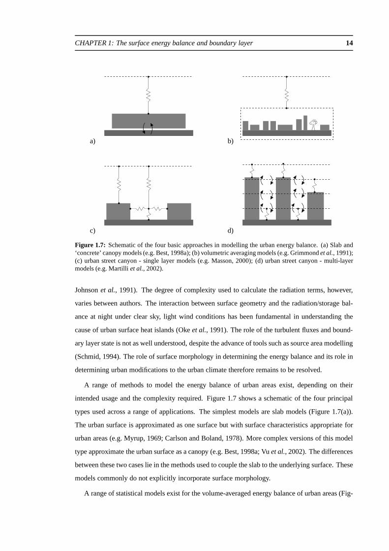
Figure 1.7: Schematic of the four basic approaches in modelling the urban energy balance. (a) Slab and‘concrete’ canopy models (e.g. Best, 1998a); (b) volumetric averaging models (e.g. Grimmondet al., 1991);(c) urban street canyon - single layer models (e.g. Masson, 2000); (d) urban street canyon - multi-layermodels (e.g. Martilliet al., 2002).
Johnsonet al., 1991). The degree of complexity used to calculate the radiation terms, however,
varies between authors. The interaction between surface geometry and the radiation/storage bal-
ance at night under clear sky, light wind conditions has beenfundamental in understanding the
cause of urban surface heat islands (Okeet al., 1991). The role of the turbulent fluxes and bound-
ary layer state is not as well understood, despite the advance of tools such as source area modelling
(Schmid, 1994). The role of surface morphology in determining the energy balance and its role in
determining urban modifications to the urban climate therefore remains to be resolved.
A range of methods to model the energy balance of urban areas exist, depending on their
intended usage and the complexity required. Figure 1.7 shows a schematic of the four principal
types used across a range of applications. The simplest models are slab models (Figure 1.7(a)).
The urban surface is approximated as one surface but with surface characteristics appropriate for
urban areas (e.g. Myrup, 1969; Carlson and Boland, 1978). More complex versions of this model
type approximate the urban surface as a canopy (e.g. Best, 1998a; Vuet al., 2002). The differences
between these two cases lie in the methods used to couple the slab to the underlying surface. These
models commonly do not explicitly incorporate surface morphology.
A range of statistical models exist for the volume-averagedenergy balance of urban areas (Fig-

CHAPTER 1: The surface energy balance and boundary layer 15
ure 1.7(b)). Most notable of these is the Objective Hysteresis Model and its successors (Grimmond
et al., 1991; Grimmond and Oke, 1999b, 2002). These models statistically parameterise the rela-
tion between the evolution of the net radiative flux and the storage terms and then subsequently
partition the residual into the turbulent fluxes. The effects of surface morphology are incorporated
into the statistically determined coefficients. The statistical determination of the model coefficients
implies that these models cannot be ported between different cities without reassessing these co-
efficients.
A number of physically based models have been developed withthe aim of incorporation into
mesoscale numerical weather prediction models. The first class of these are single layer models.
These use a generic unit of the urban surface placed entirelybelow the level of the lowest atmo-
spheric model level (Figure 1.7(c)). The majority of these models use the urban street canyon as
the generic unit of the urban surface (e.g. Masson, 2000) though arrays of cubes have been used
(e.g. Kawai and Kanda, 2003). The urban energy balance is comprised of the averaged energy
balance of (the parts of) the individual building facets. The effects of surface morphology on the
energy balance of the individual building facets and the entire urban energy balance is explicitly
incorporated in the formulation of the terms of the energy balance. This is the approach taken in
this thesis.
The final type of model (Figure 1.7(d)) also uses a generic unit of the urban surface but allows
the unit to intersect several atmospheric model levels (e.g. Martilli et al., 2002; Martilli, 2002).
The influence of the urban surface is then spread in the vertical in a more realistic way. Again the
influence of surface morphology is incorporated explicitly. In both of the final cases the morpho-
logical properties of the surface used represent the average of these properties on a spatial scale
appropriate to the resolution of the mesoscale model, i.e. the neighbourhood or city scales, so these
models cannot in practice capture the fine detail of the surface.
Three issues apply to all of these models. Firstly, the turbulent fluxes determine the coupling
of the surface and the boundary layer but their dependence onsurface morphology and boundary
layer stability is not well known or understood. Given that most observations are taken in the
atmosphere this is serious obstacle to the realistic validation of models of the urban energy balance.
Secondly, these models require a number of input parameters(e.g. surface heat capacities). It is
not known how many of these parameters relate to the observable quantities on the ground. This
is especially important given the different scales on whichthe surface properties vary and on
which these models are likely to be employed. Finally, few ofthese models have been run, and
CHAPTER 1: The surface energy balance and boundary layer 16
subsequently validated, in conjunction with boundary layer models. Given the coupled nature of
the boundary layer and energy balance the sensitivity of these models, to surface morphology for
instance, may differ when run in the coupled and surface onlysenses. This work addresses some
of these issues.
Thesis structure
This present study focusses on the influence of surface morphology on the energy balance and
boundary layer of urban areas. The aims of this work are three-fold:
To investigate the impacts of surface morphology on all parts of the surface energy balance
and boundary layer.
To determine which of the urban modifications to the local climate can be attributed to the
combined effects of surface morphology and to suggest physical explanations for those that
cannot, and finally
to determine methods to incorporate surface morphology into operational numerical weather
prediction models.
Two approaches are used to investigate these aims. Firstly,analytic, experimental and process
based modelling is used to investigate the morphological dependence of the individual terms of
the urban energy balance. Secondly, numerical studies are used to assess the impact of the effects
of surface morphology on the boundary layer.
In more detail:
Chapter 2 considers the impact of surface geometry on the exchange of diffuse radiation in
the canopy layer. A simple model to calculate net radiative flux densities is presented and
compared to commonly used alternatives.
Chapter 3 considers the impact of surface morphology on the turbulent fluxes of scalars
from an urban surface. Wind tunnel experiments and modelling are used to highlight the
important physical processes governing the turbulent transport.
Results from the previous chapters are used to formulate an urban energy balance model in
Chapter 4. The urban energy balance is comprised of the facet-averaged energy balances

CHAPTER 1: The surface energy balance and boundary layer 17
for the four facets of an urban street canyon. This energy balance model is then coupled to
a one dimensional boundary layer model, and numerical studies are used to investigate the
full impacts of surface morphology on the urban energy balance and boundary layer.
Chapter 5 considers the degree of complexity needed within the urban energy balance
model. The urban energy balance model developed in Chapter 4is compared to two ap-
proximate models which could be implemented into operational weather prediction models.
Chapter 6 considers the importance of advection in determining the urban modifications to
the local climate. Numerical simulations incorporating the advection of a boundary layer
from a rural site to an urban site are compared to previous results with a particular emphasis
on the maintenance of positive nocturnal sensible heat fluxes.
Chapter 7 summarises and discusses the results of the work and gives suggestions for future
work, noting areas of uncertainties.
The two appendices give details of the methods used to calculate the solar radiative forcing
in the thesis (Appendix A) and the turbulence closure methodused in the boundary layer
model in Chapters 4, 5 and 6 (Appendix B).
At all points the results of the work are related to observations within urban areas and the impli-
cations for operational numerical weather prediction models are highlighted.

CHAPTER TWO
Radiative exchange in an urban street canyon
2.1 Introduction
The effect of surface morphology on the radiation balance isa key to understanding the energy
balance of an urban area. The associated reduction in nocturnal radiative cooling is a principal
reason for urban-rural night time surface temperature differences (Oke, 1987; Okeet al., 1991).
However, quantitative evaluation of the radiation balancein an urban area is complicated in three
main ways. Firstly, the heterogeneity of building size, orientation and surface material proper-
ties makes the establishment of bulk properties such as the emissivity of the urban area difficult.
Secondly, geometry alters the magnitude of the incoming fluxes through a variety of processes.
Thirdly, (multiple) reflections of radiation may be an important part of the radiation balance of an
urban area unlike that of a horizontal surface.
The urban street canyon (Nunez and Oke, 1977) is often used asthe generic unit of the urban
surface within many surface energy balance models for urbanareas (Arnfield, 1982; Johnsonet al.,
1991; Mills, 1993; Sakakibara, 1996; Arnfield and Grimmond,1998; Arnfield, 2000; Masson,
2000; Kusakaet al., 2001). Even for a simple morphological construct such as the urban street
canyon there are differences in how the radiation balance has been calculated. The radiation
balance for the mid-points on each building facet can be formulated and used as representative of
the building facets (Johnsonet al., 1991). This method has the advantage of ease of validation.
The average radiation balance for (parts of) the building facets (area averages) can be formulated
(Verseghy and Munro, 1989 a,b; Kobayashi and Takamura, 1994; Masson, 2000; Kusakaet al.
2001) and used as representative of the total effect of the building facets. This method better
conserves total energy. In both cases, a range of methods areused to calculate the radiative transfer.
Reflected radiation has been observed to lead to secondary peaks in the net radiation received
18

CHAPTER 2: Radiative exchange in an urban street canyon 19
at the two walls of an urban canyon (Nunez and Oke, 1977). There are a variety of methods
used to calculate these reflections, and in the number of reflections considered, for both short-
wave and longwave radiation. Common methods include ignoring all reflections (Noilhan, 1981;
Sakakibara, 1996) or considering only one reflection (Johnson et al., 1991; Kobayashi and Taka-
mura, 1994; Masson, 2000 - longwave part; Kusakaet al., 2001). More complex methods include
increasing the number of reflections considered until convergence of the net radiation (Arnfield,
1982), solving the full geometric series (Verseghy and Munro, 1989 a,b; Masson, 2000 - shortwave
radiation) or performing Monte Carlo simulations of the path of photons in the canyon (Aida and
Gotoh, 1982; Kobayashi and Takamura, 1994; Pawlak and Fortuniak, 2002).
Verseghy and Munro (1989 a,b) showed, for two cases, that neglecting canyon geometry, multi-
ple reflections, and additional physics such as the absorption, emission and scattering of radiation
within the canyon and the non-isotropy of diffuse solar radiation could lead to appreciable errors
in the radiation terms for an urban street canyon. By comparing Monte Carlo simulations and a
one reflection model, Kobayashi and Takamura (1994) showed that the effects of reflections were
more important at higher aspect ratios and lower emissivities. Pawlak and Fortuniak (2002) show
that Monte Carlo simulations and solving the full geometricseries give similar results for a specific
case. Johnsonet al. (1991) show that the error associated with ignoring two or more reflections in
a closed system of isothermal surfaces with identical emissivities is 0.3% at an emissivity of 0.95.
However, a careful consideration of the errors resulting from neglecting reflections of radiation for
a full range of cases is needed.
In summary, there exists a range of methods to calculate the net radiation of an urban area,
particularly those based on the urban street canyon, but there is little knowledge of which approx-
imations are required across the wide range of surface parameters encountered in an urban area.
In particular, how do these methods compare across a range ofurban geometries and material
properties? This knowledge is needed to determine when eachof these methods is valid and what
complexity of solution is needed especially given the need to keep the numerical complexity of
surface energy balance models as low as possible.
Hence this chapter focusses on the exchange of diffuse radiation within an urban canyon to
establish when commonly used methods are valid. A generic method is introduced for the full
solution of the exchange of diffuse radiation in a closed system of surfaces, developed originally by
Sparrow and Cess (1970) and applied to an urban street canyonby Verseghy and Munro (1989 a,b)
and Pawlak and Fortuniak (2003). To isolate the effects of reflections, the effects of absorption,

CHAPTER 2: Radiative exchange in an urban street canyon 20
emission and scattering of radiation by the canyon volume air, and hence the dependence of the
radiation balance on the full surface energy balance, are not considered. For the purposes of this
chapter the solution calculated with the Sparrow and Cess (1970) method is taken to be the ‘exact’
solution. Two commonly used approximations, no reflectionsand one only reflection of radiation,
are compared to this exact solution over a range of canyon aspect ratios and surface material
properties. Comparison of results obtained with the three methods allows an assessment of the
applicability of the approximations.
2.2 Methodology
Sparrow and Cess (1970) have developed a method to find the solution to the diffuse radiative
exchange between the facets of closed system of surfaces surrounding a non-absorbing medium.
This method is applied here to an urban street canyon which istaken as the generic unit of the
urban surface. The radiative flux densities are assumed to beuniform across each of the surfaces.
The emission and reflection of radiation is assumed to be diffuse and according to the surface
material emissivity and albedo. The medium between the surfaces is assumed to be radiatively
non-absorbing. The exchange of longwave radiation and the diffuse component of the shortwave
radiation within an urban street canyon can be calculated using this method provided the facet-
averaged fluxes are considered. The direct component of the solar radiation cannot be calculated
using this method, but reflections of the direct component ofsolar radiation can.
The absorption, emission and scattering of radiation by theair can be significant even over the
moderately short distances within an urban canyon (Verseghy and Munro, 1989 a,b). A full radia-
tion model may be needed to account for these processes. Thischapter, however, concentrates on
the impact of reflections on the radiation balance so these processes are neglected here. Nakamura
and Oke (1988) and Voogt and Oke (1998) show that the surface temperature may not be uniform
across the individual facets of an urban street canyon. However, the relative change in surface tem-
perature across a facet is small so that the facet averaging and radiation balance calculations can
be interchanged without imposing a large error (≈ 0.3% for a±5K variation across each facet).
CHAPTER 2: Radiative exchange in an urban street canyon 21
2.3 Exchange of diffuse radiation
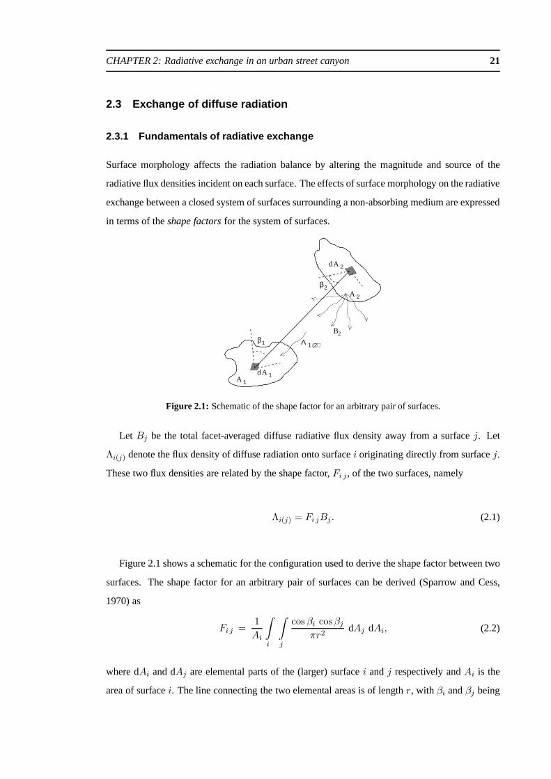
2.3.1 Fundamentals of radiative exchange
Surface morphology affects the radiation balance by altering the magnitude and source of the
radiative flux densities incident on each surface. The effects of surface morphology on the radiative
exchange between a closed system of surfaces surrounding a non-absorbing medium are expressed
in terms of theshape factorsfor the system of surfaces.
Aβ
2
2
2
1A
dA
dA 1
β1
2B
Λ 1 (2)
Figure 2.1: Schematic of the shape factor for an arbitrary pair of surfaces.
Let Bj be the total facet-averaged diffuse radiative flux density away from a surfacej. Let
Λi(j) denote the flux density of diffuse radiation onto surfacei originating directly from surfacej.
These two flux densities are related by the shape factor,Fi j, of the two surfaces, namely
Λi(j) = Fi jBj. (2.1)
Figure 2.1 shows a schematic for the configuration used to derive the shape factor between two
surfaces. The shape factor for an arbitrary pair of surfacescan be derived (Sparrow and Cess,
1970) as
Fi j =1
Ai
∫
i
∫
j
cos βi cosβj
πr2dAj dAi, (2.2)
where dAi and dAj are elemental parts of the (larger) surfacei andj respectively andAi is the
area of surfacei. The line connecting the two elemental areas is of lengthr, with βi andβj being
CHAPTER 2: Radiative exchange in an urban street canyon 22
the angles between this line and the normals to the surfaces dAi and dAj respectively.Fi j is a
function of the separation and relative orientation of the two surfacesi andj only.
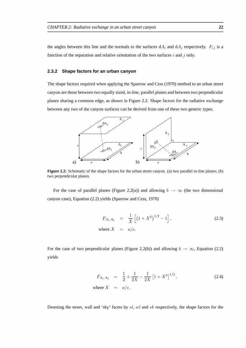
2.3.2 Shape factors for an urban canyon
The shape factors required when applying the Sparrow and Cess (1970) method to an urban street
canyon are those between two equally sized, in-line, parallel planes and between two perpendicular
planes sharing a common edge, as shown in Figure 2.2. Shape factors for the radiative exchange
between any two of the canyon surfaces can be derived from oneof these two generic types.
a)
1A
1dA
2AdA2
a
b
c
b)
1dAb
a
c1A
2dA
2A
Figure 2.2: Schematic of the shape factors for the urban street canyon. (a) two parallel in-line planes; (b)two perpendicular planes.
For the case of parallel planes (Figure 2.2(a)) and allowingb → ∞ (the two dimensional
canyon case), Equation (2.2) yields (Sparrow and Cess, 1970)
FA1 A2=
1
X
[
(
1 +X2)1/2
− 1]
, (2.3)
whereX = a/c.
For the case of two perpendicular planes (Figure 2.2(b)) andallowing b → ∞, Equation (2.2)
yields
FA1 A2=
1
2+
1
2X−
1
2X
[
1 +X2]1/2
, (2.4)
whereX = a/c.
Denoting the street, wall and ‘sky’ facets byst, wl andsk respectively, the shape factors for the
CHAPTER 2: Radiative exchange in an urban street canyon 23
urban street canyon system are then determined from Equations (2.3) and (2.4) as
Fsk st = Fst sk =
(
1 +
(
he
we
)2)
1
2
−he
we, (2.5)
Fw1 w2 =
(
1 +
(
we
he
)2)
1
2
−we
he, (2.6)
Fst w1 =1
2(1 − Fst sk), (2.7)
Fw1 st = Fw1 sk =1
2(1 − Fw1 w2). (2.8)
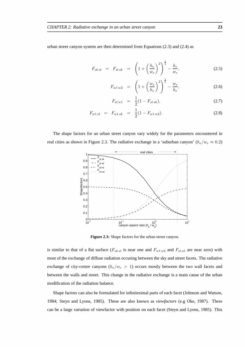
The shape factors for an urban street canyon vary widely for the parameters encountered in
real cities as shown in Figure 2.3. The radiative exchange ina ‘suburban canyon’ (he/we ≈ 0.2)
10-2
10-1
100
101
0
0.1
0.2
0.3
0.4
0.5
0.6
0.7
0.8
0.9
1
canyon aspect ratio (he / w
e)
Sha
pefa
ctor
s
Fst sk
Fst wl
Fwl st
Fwl wl
real cities
Figure 2.3: Shape factors for the urban street canyon.
is similar to that of a flat surface (Fsk st is near one andFw1 w2 andFst wl are near zero) with
most of the exchange of diffuse radiation occuring between the sky and street facets. The radiative
exchange of city-centre canyons (he/we > 1) occurs mostly between the two wall facets and
between the walls and street. This change in the radiative exchange is a main cause of the urban
modification of the radiation balance.
Shape factors can also be formulated for infinitesimal partsof each facet (Johnson and Watson,
1984; Steyn and Lyons, 1985). These are also known asviewfactors(e.g Oke, 1987). There
can be a large variation of viewfactor with position on each facet (Steyn and Lyons, 1985). This
CHAPTER 2: Radiative exchange in an urban street canyon 24
highlights the need to use the facet averaged shape factors and not representative points within
energy balance calculations. The small relative variationin surface temperature across each facet
implies that the combination of varying shape factor and surface temperature does not produce
large errors when the facet averaging and radiation balancecalculations are interchanged (≈ 1%).
2.3.3 Exact solution
The exact solution to the exchange of diffuse radiation within a closed system of surfaces is cal-
culated by developing a system of equations for the total radiative flux density away from each of
the surfaces (Sparrow and Cess, 1970). The exact method is illustrated here in the context of the
longwave radiation; the shortwave radiation is analogous with (1 − αi) replacingεi throughout;
hereεi is the surface emissivity,αi the surface albedo (full details in Sparrow and Cess (1970)).
There are a range of radiative flux densities on theith facet; the emitted,Ωi, total incoming,Λi,
total outgoing,Bi. and net,Qi. These flux densities are related by
Λi =∑
j
Fi jBj , (2.9)
Bi = Ωi + (1 − εi)Λi, (2.10)
Qi = Λi −Bi. (2.11)
The quantity of interest, namely the net component of the radiation for theith facet,Qi, in-
volves the total outgoing radiation from the other facets, i.e. all of theBj ’s.
Here the Equations (2.9)-(2.11) are solved by expressing them in matrix form, namely
Bi = Ωi + (1 − εi)∑
j
Fi jBj , (2.12)
Ωi =∑
j
ΓijBj, (2.13)
whereΓij = δij − (1 − εi)Fi j .
Since the matrixΓij always has an inverse,ψij , Equation (2.13) can be inverted to give the

CHAPTER 2: Radiative exchange in an urban street canyon 25
total outgoing radiative flux density, and hence the net radiative flux density, for each facet,
Bi =∑
j
ψijΩj , (2.14)
Qi =
∑
jFi jBj − Ωi, if εi = 1,
(εiBi − Ωi)/(1 − εi), otherwise.
(2.15)
The matrixΓ is inverted numerically for each value ofhe/we andεi. Equation (2.15) can be
expressed in matrix form for ease of use as part of a surface energy balance model.
2.3.4 Approximate solutions
Most previous studies have developed approximate solutions to Equations (2.9)-(2.11). Equations
(2.9) and (2.10) show that the net radiative flux density for aparticular facet is an infinite geometric
series in(1 − ε). Previous studies approximate this infinite series by truncating after a finite
number of terms. Noilhan (1981) neglects all reflections; whereas Kusakaet al. (2001) retains
only one reflection. Ignoring all reflections (denotedR0) is formally the approximation resulting
from ignoring all terms of order(1 − ε) and higher. Retaining only one reflection (denotedR1)
is formally the approximation resulting from ignoring all terms of order(1 − ε)2 and higher. The
corresponding forms of Equation (2.15) after these approximations have been made are
R0 : Q0i = εi
∑
j
Fi jΩj − Ωi, (2.16)
R1 : Q1i = εi
∑
j
Fi j
(
Ωj + (1 − εi)∑
k
Fj kΩk
)
− Ωi. (2.17)
2.3.5 Application to the urban street canyon
The application of the three methods to an urban street canyon requires the specification of the
emitted flux densities and emissivities for each of the facets of the canyon system. The emitted
flux density from each of the canyon facets is calculated using Stefan’s law (top line Equation
(2.18) below). The emissivity of the sky facet is one and the emitted flux density for the sky

CHAPTER 2: Radiative exchange in an urban street canyon 26
facet is the downwelling longwave radiationL↓. With these specifications, consider again the
approximate solutions given in Section 2.3.4. The emitted flux densities from the canyon facets
are of orderε and the downwelling longwave radiation is of order one. Equations (2.16) and (2.17)
must then be adapted to keep the approximations consistent in powers ofε. To do this an extra
reflection of the downwelling radiation must be retained compared to the number of reflections
of the radiation emitted from the canyon facets. The consistent approximate solutions for the net
radiation are then
Ωi =
εiσT4 for i = st, wl
L↓ for i = sk
, (2.18)
Q0i = εi
∑
j
Fi j (Ωj + (1 − εj)Fj skL↓) − Ωi, (2.19)
Q1i =
εi∑
jFi j Ωj − Ωi +
εi∑
jFi j(1 − εj)
(
∑
k
Fj k (Ωk + (1 − εk)Fk skL↓)
) . (2.20)
Note, obviously, all solutions agree whenεi = 1 for all surfaces. Comparison of the three solu-
tions, namely Equations (2.15), (2.19) and (2.20), are shown next.
2.4 Comparison of the exact solution with the approximation s
A comparison of results for the net longwave radiation,Qi, for each facet from an individual case
is now considered. The absolute values and differences between the three methods depend on
the case considered but the features highlighted are robust. Consider the particular case when the
emitted flux densities are prescribed by setting the facet surface temperatures at 295 K and the
downwelling longwave radiation is 275 W m−2 . These values are chosen to be realistic for mid-
latitude regions. Each of the canyon facets has the same emissivity. Results are described for a
range of canyon aspect ratios,he/we, and emissivities,ε.
2.4.1 Exact solution - longwave radiation
The net radiative flux density from the canyon facets gives a measure of how the surface temper-
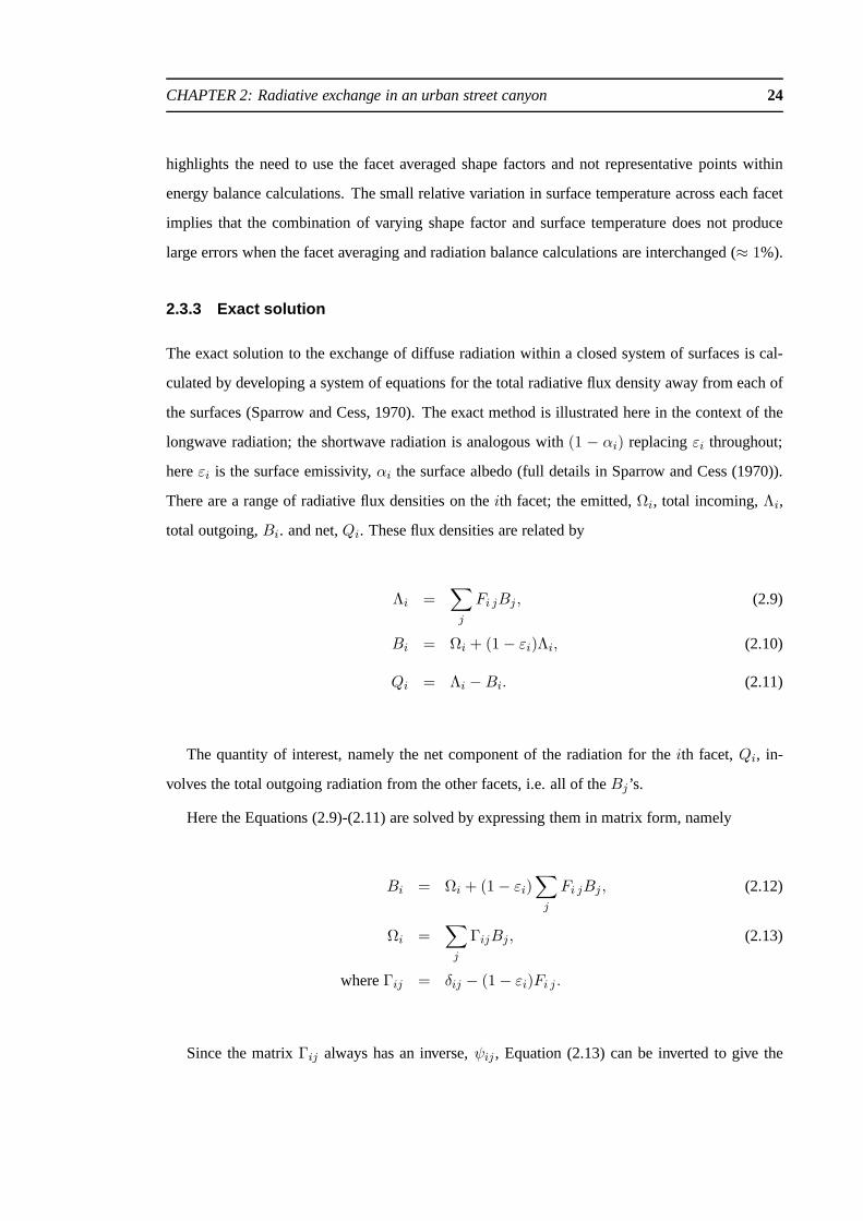
atures of the canyon facets would change for the case considered. Figure 2.4 shows the weighted
CHAPTER 2: Radiative exchange in an urban street canyon 27
(by surface area) average of the net radiative flux density for the three canyon facets calculated
using the exact solution. Note the tendency towards the flat case as the canyon aspect ratio de-
creases, the tendency to zero net radiation whenε → 0 and the decrease in the magnitude of the
net radiative flux density as the aspect ratio increases. Thetransition between a net radiative flux
density which is close to that of a flat surface to that of a highly convoluted surface is rapid around
he/we = 0.5 . This illustrates the large impact that surface geometry has on the net radiative flux
density and thus the sensitivity to geometry of the radiation balance of the urban street canyon.
The range of emissivities for natural materials isε > 0.5 .
10-2
10-1
100
101
0
0.1
0.2
0.3
0.4
0.5
0.6
0.7
0.8
0.9
1
canyon aspect ratio (he/w
e)
Mat
eria
l em
issi
vity
-20
-60
-100
-140
Figure 2.4: Weighted by surface area average of the net longwave radiative flux density from the threecanyon facets using the exact solution - contours every 10 W m−2 from -150 to -10 W m−2 (light).
10-2
10-1
100
101
0
0.1
0.2
0.3
0.4
0.5
0.6
0.7
0.8
0.9
1
canyon aspect ratio (he/w
e)
Mat
eria
l em
issi
vity
0.7
0.9
0.99
Figure 2.5: Canyon top net radiative flux density normalised by the net radiative flux density of a horizontalblackbody surface - contours every 0.1 from 0.1 (dark) to 0.9then 0.95 and 0.99 (light).
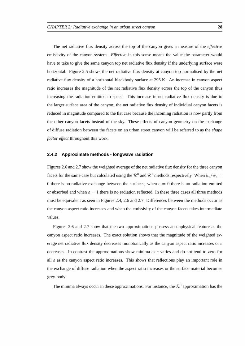
CHAPTER 2: Radiative exchange in an urban street canyon 28
The net radiative flux density across the top of the canyon gives a measure of theeffective
emissivity of the canyon system.Effectivein this sense means the value the parameter would
have to take to give the same canyon top net radiative flux density if the underlying surface were
horizontal. Figure 2.5 shows the net radiative flux density at canyon top normalised by the net
radiative flux density of a horizontal blackbody surface at 295 K. An increase in canyon aspect
ratio increases the magnitude of the net radiative flux density across the top of the canyon thus
increasing the radiation emitted to space. This increase innet radiative flux density is due to
the larger surface area of the canyon; the net radiative flux density of individual canyon facets is
reduced in magnitude compared to the flat case because the incoming radiation is now partly from
the other canyon facets instead of the sky. These effects of canyon geometry on the exchange
of diffuse radiation between the facets on an urban street canyon will be referred to as theshape
factor effectthroughout this work.
2.4.2 Approximate methods - longwave radiation
Figures 2.6 and 2.7 show the weighted average of the net radiative flux density for the three canyon
facets for the same case but calculated using theR0 andR1 methods respectively. Whenhe/we =
0 there is no radiative exchange between the surfaces; whenε = 0 there is no radiation emitted
or absorbed and whenε = 1 there is no radiation reflected. In these three cases all three methods
must be equivalent as seen in Figures 2.4, 2.6 and 2.7. Differences between the methods occur as
the canyon aspect ratio increases and when the emissivity ofthe canyon facets takes intermediate
values.
Figures 2.6 and 2.7 show that the two approximations possessan unphysical feature as the
canyon aspect ratio increases. The exact solution shows that the magnitude of the weighted av-
erage net radiative flux density decreases monotonically asthe canyon aspect ratio increases orε
decreases. In contrast the approximations show minima asε varies and do not tend to zero for
all ε as the canyon aspect ratio increases. This shows that reflections play an important role in
the exchange of diffuse radiation when the aspect ratio increases or the surface material becomes
grey-body.
The minima always occur in these approximations. For instance, theR0 approximation has the
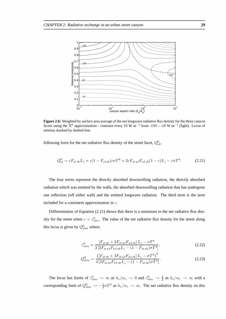
CHAPTER 2: Radiative exchange in an urban street canyon 29
10-2
10-1
100
101
0
0.1
0.2
0.3
0.4
0.5
0.6
0.7
0.8
0.9
1
canyon aspect ratio (he/w
e)
Mat
eria
l em
issi
vity
-20
-60
-100
-140
-100
Figure 2.6: Weighted by surface area average of the net longwave radiative flux density for the three canyonfacets using theR0 approximation - contours every 10 W m−2 from -150 – -10 W m−2 (light). Locus ofminima marked by dashed line.
following form for the net radiative flux density of the street facet,Q0st,
Q0st = εFst skL↓ + ε(1 − Fst sk)εσT
4 + 2εFst wlFwl sk(1 − ε)L↓ − εσT 4. (2.21)
The four terms represent the directly absorbed downwellingradiation, the directly absorbed
radiation which was emitted by the walls, the absorbed downwelling radiation that has undergone
one reflection (off either wall) and the emitted longwave radiation. The third term is the term
included for a consistent approximation inε.
Differentiation of Equation (2.21) shows that there is a minimum in the net radiative flux den-
sity for the street whenε = ε0stm. The value of the net radiative flux density for the street along
this locus is given byQ0stm where,
ε0stm =[Fst sk + 2Fst wlFwl sk]L↓ − σT 4
2 [2Fst wlFwl skL↓ − (1 − Fst sk)σT 4], (2.22)
Q0stm =
(
[Fst sk + 2Fst wlFwl sk]L↓ − σT 4)2
4 [2Fst wlFwl skL↓ − (1 − Fst sk)σT 4]. (2.23)
The locus has limits ofε0stm → ∞ ashe/we → 0 andε0stm → 12 ashe/we → ∞ with a
corresponding limit ofQ0stm → −1
4σT4 ashe/we → ∞. The net radiative flux density on this
CHAPTER 2: Radiative exchange in an urban street canyon 30
10-2
10-1
100
101
0
0.1
0.2
0.3
0.4
0.5
0.6
0.7
0.8
0.9
1
canyon aspect ratio (he/w
e)
Mat
eria
l em
issi
vity
-20
-60
-100
-140 -20
Figure 2.7: Weighted by surface area average of the net longwave radiative flux density for the three canyonfacets using theR1 approximation - contours every 10 W m−2 from -150 to -10 W m−2 (light). Locus ofminima marked by dashed line; locus of maxima marked by dotted line (real-only parts shown).
locus is incorrect as the canyon aspect ratio increases. Theinclusion of the additional term to keep
a consistent cutoff inε does not affect this result qualitatively.
Similar analysis of the net radiative flux density for the walls, Q0wl, shows a similar locus of
minima. The net radiative flux density for the wall facets on this locus is the same as that of the
street facet on the locusε0stm whenhe/we → ∞. As the canyon aspect ratio becomes small the
limits on the locus areε0wlm → 1 andQ0wlm → 1
2(L↓ − σT 4) which is correct. The weighted
average net radiative flux density for the three canyon facets will therefore also always have a
locus of minima, as is shown in Figure 2.6. The locus marks theminima when varyingε, i.e. it
will cross contours of the net radiative longwave flux density when these contours are parallel to
theε axis.
The minimum for theR1 method affects a smaller range of canyon aspect ratios than that of the
R0 method. The cubic nature of the expressions forQ1st andQ1
wl resists similar simple analysis
(Abaramowitz and Stegun, 1973) but gives loci of minima and maxima as shown in Figure 2.7.
2.4.3 Errors of the approximate solutions
Figures 2.8 and 2.9 show the relative error of theR0 andR1 methods, respectively, compared
to the exact solution. The relative error is chosen as this measure of the error is not particular to
the case considered here. The approximate methods always overestimate the magnitude of the net

CHAPTER 2: Radiative exchange in an urban street canyon 31
radiative flux and can be an order of magnitude incorrect. Fortypical emissivities, e.g.ε = 0.9,
theR0 method can be 10% or more incorrect, theR1 method 5% or more incorrect. As expected
theR1 method is the better approximation for all canyon aspect ratios and emissivities.
10-2
10-1
100
101
0
0.1
0.2
0.3
0.4
0.5
0.6
0.7
0.8
0.9
1
canyon aspect ratio (he/w
e)
Mat
eria
l em
issi
vity
0.01 0.05 0.1 0.3 1.0 2.0
Figure 2.8: Relative error of the weighted average of net radiative flux density using theR0 approximation- contours at 0.01 (dark), 0.05, every 0.1 from 0.1–1.0 then every 1.0.
10-2
10-1
100
101
0
0.1
0.2
0.3
0.4
0.5
0.6
0.7
0.8
0.9
1
canyon aspect ratio (he/w
e)
Mat
eria
l em
issi
vity
0.01 0.05 0.1 0.3 1.0 2.0
Figure 2.9: Relative error of the weighted average of net radiative flux density using theR1 approximation- contours at 0.01 (dark), 0.05, every 0.1 from 0.1–1.0 then every 1.0.
The errors of the approximations are very sensitive to the material emissivity in the range of
realistic emissivities (e.g. 0.7 – 0.9 for concrete,≈ 0.95 for asphalt, Oke (1987)). For instance,
the relative error of theR0 method at a canyon aspect ratio ofhe/we = 1 and ε = 0.95 is
20%. A small uncertainty in the emissivity of the material property,ε = 0.95 ± 0.02, leads to
CHAPTER 2: Radiative exchange in an urban street canyon 32
a range of relative errors of 10–30%. A small uncertainty in the surface material emissivity can
therefore have an unphysically large impact on the accuracyof the net radiation calculations if
these approximations are used.
The loci of minima from the two methods give natural conditions for when the approximations
can be considered to be valid. Regions ofhe/we − ε space which show these unphysical features
are where the approximate methods deviate significantly from the exact solution. Although these
are case dependent, broad conclusions are that theR0 method should not be used for canyon
aspect ratios greater than 0.3, theR1 method should not be used for canyon aspect ratios greater
than 0.8. Additionally the dependence of the relative errorof the two methods on the material
emissivity suggests that these thresholds should be lowered when considering materials with a
low emissivity. For full applicability only the exact solution is valid.
Allowing the emissivity of the different facets to vary fromeach other does not qualitatively
change these relative error patterns. The approximations continue to perform well for high emis-
sivities and low canyon aspect ratios. For lower emissivities and higher aspect ratios the relative
error of each approximation is close to but greater than the relative error of the approximation
when applied to the same street canyon but with all the facetshaving the emissivity of the surface
with the highest emissivity.
2.4.4 Shortwave radiation
The method of Sparrow and Cess (1970) assumes the flux densities on each surface are uniform.
Hence this method is not applicable to the direct component of the solar radiation because the
direct component experiences shadowing and therefore the flux densities on each facet are not uni-
form. Instead, standard solar geometry schemes (e.g. Owczarek, 1997) and a shadowing scheme
(e.g. Swaid, 1993; Sakakibara, 1996) can be used to calculate the facet-averaged direct solar ra-
diative flux densities as described in Appendix A. When such geometric effects are considered,
the flux densities depend on time, location and canyon orientation, and so do the relative errors in
neglecting reflections (Verseghy and Munro, 1989a). The Sparrow and Cess method can be ap-
plied however to the diffuse component of the incoming shortwave radiation and to any diffusely
reflected solar radiation. A similar method to that illustrated here has been used successfully to
predict the time variation of the effective albedo of an urban street canyon (Pawlak and Fortuniak,
2003).
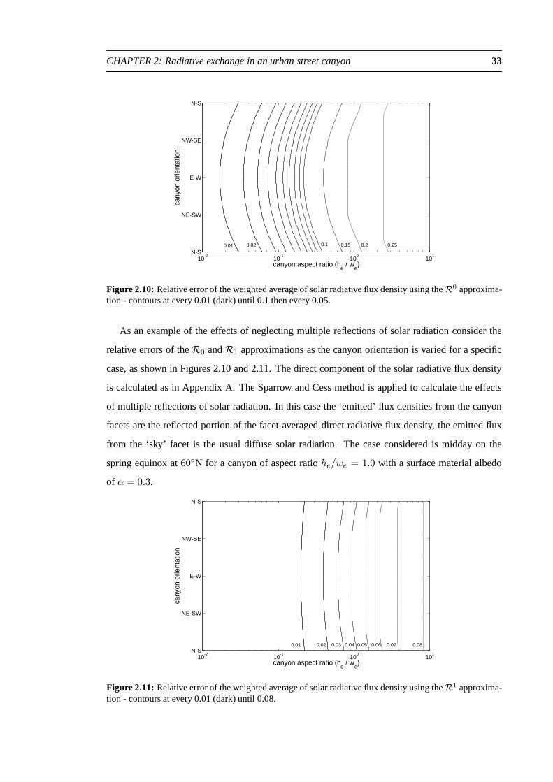
CHAPTER 2: Radiative exchange in an urban street canyon 33
10-2
10-1
100
101
N-S
NE-SW
E-W
NW-SE
N-S
canyon aspect ratio (he / w
e)
cany
on o
rient
atio
n
0.250.20.150.10.020.01
Figure 2.10:Relative error of the weighted average of solar radiative flux density using theR0 approxima-tion - contours at every 0.01 (dark) until 0.1 then every 0.05.
As an example of the effects of neglecting multiple reflections of solar radiation consider the
relative errors of theR0 andR1 approximations as the canyon orientation is varied for a specific
case, as shown in Figures 2.10 and 2.11. The direct componentof the solar radiative flux density
is calculated as in Appendix A. The Sparrow and Cess method isapplied to calculate the effects
of multiple reflections of solar radiation. In this case the ‘emitted’ flux densities from the canyon
facets are the reflected portion of the facet-averaged direct radiative flux density, the emitted flux
from the ‘sky’ facet is the usual diffuse solar radiation. The case considered is midday on the
spring equinox at 60N for a canyon of aspect ratiohe/we = 1.0 with a surface material albedo
of α = 0.3.
10-2
10-1
100
101
N-S
NE-SW
E-W
NW-SE
N-S
canyon aspect ratio (he / w
e)
cany
on o
rient
atio
n
0.01 0.02 0.03 0.04 0.05 0.06 0.07 0.08
Figure 2.11:Relative error of the weighted average of solar radiative flux density using theR1 approxima-tion - contours at every 0.01 (dark) until 0.08.

CHAPTER 2: Radiative exchange in an urban street canyon 34
With both methods the relative error is dependent on the orientation of the canyon. Both ap-
proximate methods perform worse for east-west orientated canyons than for north-south orientated
canyons. This is due to the asymmetry of the direct forcing onthe two walls present at this time.
Comparing the two figures shows that most of the inaccuracy isdue to the first reflection of ra-
diation. The error due to variation of the canyon orientation remains a second order effect with
the canyon aspect ratio and surface material albedo being the dominant parameters controlling the
accuracy of the two approximate methods.
The same conclusions on the validity of the different approximations remains, with the condi-
tions on the material emissivity,ε being replaced by equivalent conditions on the material albedo,
α. The increased magnitude of the solar radiation (of typicalmagnitude 0 to 1000 W m−2), com-
pared to the net longwave radiation (of typical magnitude -200 to -50 W m−2), would suggest
that a more accurate solution is required for the solar radiation and therefore the exact solution is
needed. Most natural materials have emissivities that are close to one but albedos have a much
greater natural range, for instance 0.2–0.4 for brick or 0.05–0.5 for glass (Oke, 1987). Reflec-
tions are therefore more likely to be important for the solarcomponent of the radiation balance
particularly as the canyon aspect ratio increases.
For example, consider a north-south orientated brick canyon (ε = 0.9, α = 0.3) of aspect
ratio 1.0 at 50N on the spring equinox. The relative error in the total solarcomponent of the
zero reflections approximation is found to be 18%, that of theone reflection approximation 2.5%.
This compares with the relative errors of the longwave radiation component, namely 30% for
the zero reflections approximation and 3% for the one reflection approximation. However, the
absolute errors for the solar component can be larger than those of the longwave component given
a reasonable solar forcing. Reflections are therefore more likely to become important for the solar
component of the radiation balance in an absolute sense eventhough the relative error may be
smaller due to the direct component of the solar radiation.
The urban street canyon absorbs more solar radiation, lowering the effective albedo of the
system as a whole, but the increase in surface area means thatthe average flux density onto the
three canyon facets is smaller than that of a horizontal surface of the same material.

CHAPTER 2: Radiative exchange in an urban street canyon 35
2.5 Summary and conclusions
The radiative exchange in an urban canyon has been investigated assuming that the radiative flux
densities are uniform along each of the facets and that radiation is emitted and reflected diffusely.
A method of calculating the exact solution to the net balancefor the different facets of the urban
canyon has been implemented and compared to two commonly used approximations. In practice
this method requires the calculation and inversion of the matrix Γ for each canyon aspect ratio and
material property considered. The coefficients in this matrix are then fixed; hence this method is
simple to execute numerically. The exact solution varies significantly from the two approximations
considered, and is therefore needed for accuracy, if the albedo of the surface material is greater than
0.2 or the emissivity is less than 0.8. Some building materials have emissivities or albedos which
would imply the need to use the exact solution, e.g. concreteε ≈ 0.7–0.9 and brickα ≈ 0.2–
0.4. The need for the more complicated approach becomes morecritical as the canyon aspect
ratio increases. Errors from the approximate methods can belarge (an order of magnitude) and
vary rapidly across the range of emissivities and albedos commonly encountered from building
materials. Uncertainty in the material properties can thenhave an unphysically large impact on
the accuracy of the net radiative flux density calculated when these approximations are used. This
method has been validated against field measurements of the solar radiation over a scaled model
of an urban street canyon (Pawlak and Fortuniak, 2003).
The exact solution is taken from a generic method and so can begeneralised to alternative
building configurations. For different geometries the shape factors between each pair of surfaces
need to be calculated. The effect of multiple reflections is then achieved by inverting matrix
equations analogous to Equations (2.12) and (2.13). Similar adaptation of the other two methods to
other building configurations would make them comparable incomplexity and hence the increased
accuracy gained would favour using the exact solution.
The radiation balance in an urban setting is highly complex.Multiple reflections are shown
here to play an important role; Verseghy and Munro (1989 a,b,) show, for a particular case, that
the errors associated with the neglect of absorption, emission and scattering of radiation by the
air in the canyon volume can be of a similar magnitude to that of neglecting multiple reflections.
Given the large errors identified here when neglecting multiple reflections, it seems likely that both
effects need to be incorporated into the radiation component of any surface energy balance model
of an urban area. Urban energy balance models based on the urban street canyon need to consider

CHAPTER 2: Radiative exchange in an urban street canyon 36
at least one reflection of radiation and multiple reflectionsare desirable for full applicability.
The surface morphology has two principal effects on the radiation balance of an urban area.
Firstly, the increase in surface area acts to decrease the average radiative flux densities which
would reduce the temperature variation at the surface. The reduction in temperature variation
observed may not be as large as expected given the change in the average flux densities due to the
asymmetry of the solar forcing resulting from shadowing. Secondly, surface geometry allows the
radiation balances of different surfaces to interact. For instance, reflected radiation can form a large
part of the incoming radiative flux density of a surface. Thiseffect means that the urban surface
as a whole absorbs from and emits more radiation to the overlying atmosphere than a flat surface
of equivalent material properties. This is despite the reduction in the flux densities at the surface.
It is this balance between the increase in surface area and effects of surface geometry which must
be preserved when incorporating urban areas into numericalweather prediction models.

CHAPTER THREE
Turbulent exchange in an urban street canyon
3.1 Introduction
The turbulent fluxes of heat, moisture and momentum play a keyrole in determining the energy
balance of any surface, and therefore in determining the surface temperature and the vertical pro-
files of the wind and temperature in the boundary layer. The building configuration of urban areas
is known to affect the radiative component of the energy balance (Arnfield, 2003) and the turbu-
lent flux of momentum (Raupachet al., 1980; Grimmond and Oke, 1999b). The sensible heat flux
from an urban area varies more spatially than the net radiative flux does over an urban area (Schmid
et al., 1991) and depends on the surface type and usage (Grimmond and Oke, 2002; Christenet al.,
2003). How this variation relates to differences in the building configuration remains unknown.
This knowledge is needed for studies of the near-surface urban air quality and the formulation of
the sensible and latent heat fluxes in surface energy balancemodels of urban areas.
The sensible heat flux is a key term in the surface energy balance. Both the surface and bound-
ary layer temperature is determined, in part, by the sensible heat flux. In particular, the evolution
and depth of the boundary layer is intimately linked to the sensible heat flux and its relation to the
latent heat flux (Raupach, 2001). The potential for feedbackbetween the surface energy balance
and the boundary layer (e.g. Brubaker and Entekhabi, 1995, 1996) implies that accuracy is needed
when calculating this term of the urban energy balance within numerical weather prediction mod-
els.
There are a range of existing models for the turbulent fluxes from urban areas, primarily as part
of models of the surface energy balance. Grimmondet al.(1991) and Grimmond and Oke (1999a)
present an urban surface energy balance model in which the flux of energy into the building fabric
and then the turbulent fluxes are related to the evolution of the net radiation. Any influence of
37

CHAPTER 3: Turbulent exchange in an urban street canyon 38
the surface morphology on the turbulent fluxes is dealt with empirically by training the model
with observations to each location. Best (1998b, 1999) takes a similar approach by modifying the
ground heat flux and allowing the turbulent fluxes to adjust accordingly. What these approaches
lack is treatment of how urban morphology affects the physical processes governing the turbulent
fluxes.
Many models of the atmospheric processes in an urban area arebased on a generic unit of
an urban area. One such generic unit is the urban street canyon (Nunez and Oke, 1977). This
generic unit is used as the basis of many energy balance models for urban areas (Johnsonet al.,
1991; Mills, 1993; Sakakibara, 1996; Arnfield and Grimmond,1998; Masson, 2000; Kusakaet al.,
2001; Martilli et al., 2002). Urban street canyon models parameterise the turbulent exchange
of heat from the canyon facets to the air above the canyon. Theparameterisation is commonly
empirical (Kusakaet al., 2001) or based on the turbulent transfer from a horizontal but rough
surface (Massonet al., 2002). Most models formulate the fluxes in terms of the wind speed within
the street canyon. A range of methods are employed to parameterise this wind speed. These
include invoking results from the studies of the flow throughvegetation canopies (Masson, 2000),
invoking continuity (Mills, 1993) and determining the vertical profile of the wind through the
accumulated effects of drag from a series of street canyons (Martilli et al., 2002). In all cases,
the parameterisation of the turbulent flux from the individual facets and the flux from the entire
canyon unit need to be validated.
The flow (Oke, 1988; Baiket al., 2000) and turbulence (Johnson and Hunter, 1995) within an
urban street canyon varies with canyon geometry. The turbulent flux of a scalar from the facets
of an urban street canyon is therefore expected to be influenced by canyon geometry. Barlow and
Belcher (2002) develop a wind tunnel method for measuring the facet-averaged flux of a passive
scalar in a neutral atmosphere from the street facet of a single urban street canyon. Barlowet al.
(2004) used this method to measure the facet-averaged flux from each of the facets of a series of
urban street canyons. Narita (2003) measured the flux of a scalar from the facets of a range of
urban canonical geometries using a similar method to Barlowand Belcher (2002). All of these
measurements showed a dependence of the fluxes on canyon geometry including a non-monotonic
variation of the flux from the street facet as the canyon aspect ratio is increased. The purpose of
this chapter is to develop a quantitative model for the turbulent flux of a scalar from an urban street
canyon that explains the dependence of the fluxes on the geometry of the street canyon that was
observed by Barlowet al. (2004).

CHAPTER 3: Turbulent exchange in an urban street canyon 39
This chapter therefore focusses on the geometric dependence of turbulent exchange from an
urban street canyon and the physical processes responsiblefor this dependence. The urban area
is represented by a series of urban street canyons oriented normally to the wind. Consideration is
focussed on the case of forced convection. A model for the facet-averaged fluxes from each facet
of an urban street canyon in neutral conditions is presentedfor a range of canyon geometries. The
model is developed from ideas on the turbulent transfer across developing boundary layers (Sec-
tion 3.2) and ideas on the geometric dependence of the flow within and above the street canyon
(Sections 3.4 and 3.5). A comparison between the model predictions and wind tunnel measure-
ments of Barlowet al. (2004) then allows an assessment of which physical processes determine
the geometric dependence of the turbulent flux of a scalar from an urban surface.
3.2 The bulk aerodynamic formulation for surface fluxes
The time- and spatially- averaged flux density of a scalar propertyX in the inertial sub-layer,FX
,
is given by
FX = 〈w′X ′〉, (3.1)
where the primes indicate the instantaneous departure fromthe mean value ofX, the over-bar
denotes a time average and the angle brackets a spatial average. If the flux ofX is mediated
entirely by turbulence, dimensional analysis shows that the flux is proportional to the difference
of the mean valuesX takes at the surface and at some height above that surface multiplied by a
transport velocity. This approach of relating the flux ofX to the mean values ofX is the bulk
aerodynamic formulation (Garratt, 1992). Denoting the area-averaged value ofX at the surface
by 〈Xs〉 and at any height,z, in the inertial sub-layer,〈X〉, the flux density ofX at the surface,
FX
, is then given by
FX
= wX
(
〈Xs〉 − 〈X〉)
=〈Xs〉 − 〈X〉
rX
, (3.2)
wherewX
is the transfer velocity for propertyX and its reciprocal,rX
, is the resistance to transport.
For a neutrally stratified rough-wall boundary layer with zero displacement height that is in
equilibrium with the underlying surface, the mean verticalwind profile,〈u(z)〉, and mean vertical

CHAPTER 3: Turbulent exchange in an urban street canyon 40
profile ofX, 〈X(z)〉, vary as
〈u(z)〉 =u∗κ
ln
(
z
z0m
)
, (3.3)
〈X(z)〉 − 〈Xs〉 =X∗
κln
(
z
z0X
)
, (3.4)
whereu∗ = (τ/ρ)1/2 is the friction velocity,X∗ = −FX/u∗ is a scaling forX ′, κ is the von
Karman constant andz0m andz
0Xare the roughness lengths for momentum and propertyX re-
spectively. The resistance to the transport ofX therefore takes the form
rX
(z) = ln
(
z
z0m
)
ln
(
z
z0X
)
/
κ2〈u(z)〉. (3.5)
Within the inertial sub-layer of the atmospheric boundary layer the area-averaged flux density
is uniform with height and therefore takes the same value as at the surface. Using Equation (3.5)
at two heights,z1 < z2, within the inertial sub-layer, the flux density ofX at the surface can be
related to the mean vertical profile ofX by
FX
= wX∆
(
〈X(z1)〉 − 〈X(z2)〉)
=〈X(z1)〉 − 〈X(z2)〉
rX
(z2) − rX
(z1). (3.6)
Using Equations (3.3), (3.4) and (3.6) the resistance to transport between the two atmospheric
levels,rX∆
= rX
(z2) − rX
(z1), can be expressed as
rX∆
=∆〈X〉
u∗X∗. (3.7)
In a boundary layer where the mean vertical profiles of all properties can be described by Equation
(3.4), as determined by the relevant roughness lengths,rX∆
takes the same value regardless of the
property considered.
A boundary layer undergoing an adjustment to new surface properties forms an internal bound-
ary layer. The profile ofX in such a region can be considered to form three sub-layers. The

CHAPTER 3: Turbulent exchange in an urban street canyon 41
inner-most layer is in full equilibrium with the underlyingsurface, the outer-most layer remains
unaffected by the change in surface properties with the middle layer blending the two profiles
together. The depth of the internal boundary and inner layers relate to the distance downstream
from the change in surface properties; the inner layer is taken to grow linearly with distance from
the surface change. The turbulent transport from the surface to a height in the outer layer depends
on both the resistance to transport off the surface,r1, and the resistance to transport across the
internal boundary layer,r12, as shown schematically in Figure 3.1. If the wind speed at height z1
in the inner layer is known,r1 is given by Equation (3.5). The resistance to transportr12 is given
by Equation (3.7) where nowu∗ andX∗ are the local scaling terms. These local scaling terms are
approximated by those of the outer layer as transport is dominated by the larger eddies which will
have this characteristic scaling.
inner layer
blending layer
outer layer
2z
1 α
x
xz
U
z z
r
r1
12
0m1 0m2
Figure 3.1: Schematic of the resistance network across a developing internal boundary layer.
In an adjusting boundary layer it is not immediately obviousthat Equation (3.7) takes the same
value for all propertiesX. In fact, assuming Equation (3.7) holds for the transport ofmomentum,
the resistance to transport of propertyX depends on the ratiorX∆/r
u∆- when considering heat
this ratio is the turbulent Prandtl number. For small scale turbulence and turbulence in a free shear
layer the turbulent Prandtl number is approximately 1 (Tennekes and Lumley, 1997, pp. 51). It
follows that the resistance to transport of heat (temperature) across a free shear layer is given by
rT∆
= ∆u/u2∗, where the friction velocity is that of the outer layer.
3.3 The naphthalene sublimation technique for scalar fluxes
Quantifying the facet-averaged scalar flux from a canyon facet is complicated in three main ways.
Firstly flux measurements need careful interpretation. Even modern measurement techniques can
requirea priori information which may not be known. For instance scintillometry, which can mea-
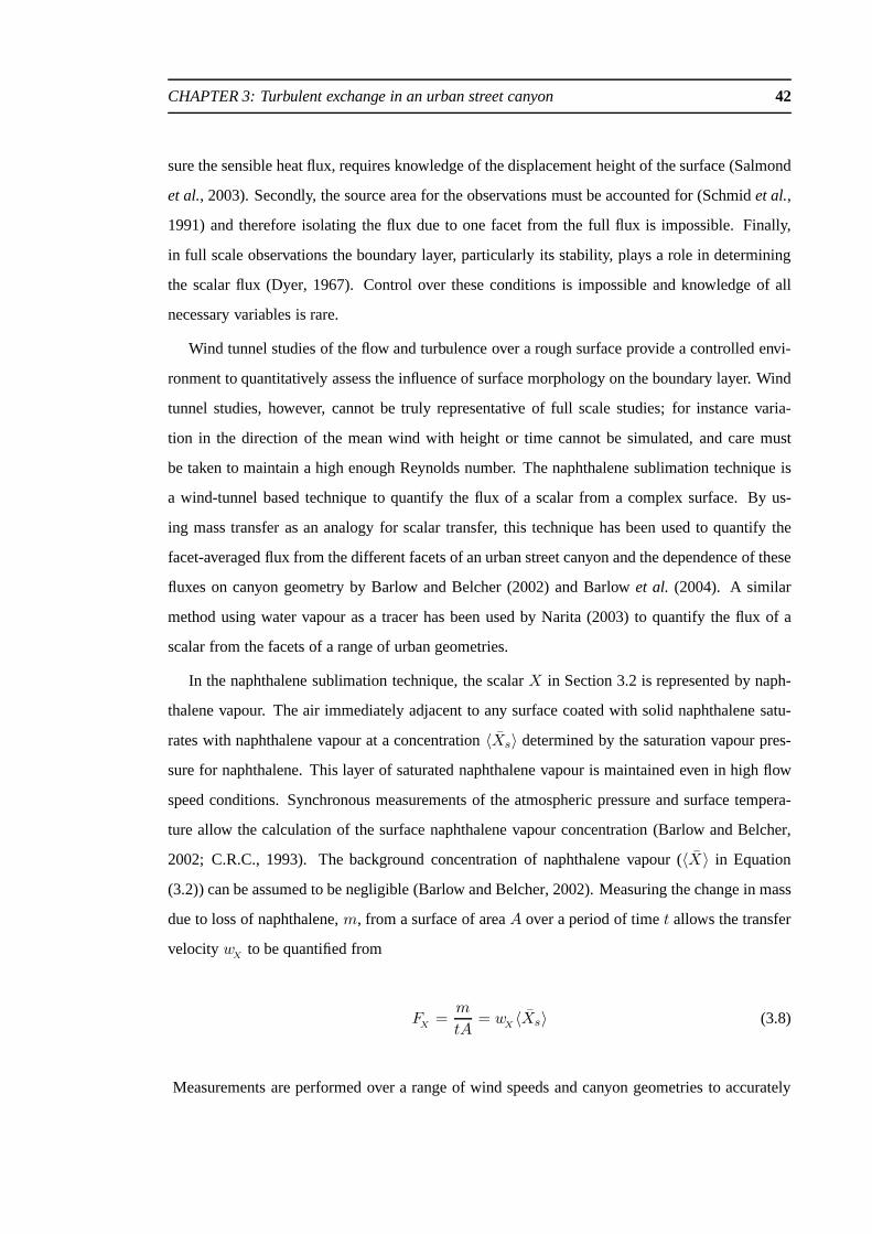
CHAPTER 3: Turbulent exchange in an urban street canyon 42
sure the sensible heat flux, requires knowledge of the displacement height of the surface (Salmond
et al., 2003). Secondly, the source area for the observations mustbe accounted for (Schmidet al.,
1991) and therefore isolating the flux due to one facet from the full flux is impossible. Finally,
in full scale observations the boundary layer, particularly its stability, plays a role in determining
the scalar flux (Dyer, 1967). Control over these conditions is impossible and knowledge of all
necessary variables is rare.
Wind tunnel studies of the flow and turbulence over a rough surface provide a controlled envi-
ronment to quantitatively assess the influence of surface morphology on the boundary layer. Wind
tunnel studies, however, cannot be truly representative offull scale studies; for instance varia-
tion in the direction of the mean wind with height or time cannot be simulated, and care must
be taken to maintain a high enough Reynolds number. The naphthalene sublimation technique is
a wind-tunnel based technique to quantify the flux of a scalarfrom a complex surface. By us-
ing mass transfer as an analogy for scalar transfer, this technique has been used to quantify the
facet-averaged flux from the different facets of an urban street canyon and the dependence of these
fluxes on canyon geometry by Barlow and Belcher (2002) and Barlow et al. (2004). A similar
method using water vapour as a tracer has been used by Narita (2003) to quantify the flux of a
scalar from the facets of a range of urban geometries.
In the naphthalene sublimation technique, the scalarX in Section 3.2 is represented by naph-
thalene vapour. The air immediately adjacent to any surfacecoated with solid naphthalene satu-
rates with naphthalene vapour at a concentration〈Xs〉 determined by the saturation vapour pres-
sure for naphthalene. This layer of saturated naphthalene vapour is maintained even in high flow
speed conditions. Synchronous measurements of the atmospheric pressure and surface tempera-
ture allow the calculation of the surface naphthalene vapour concentration (Barlow and Belcher,
2002; C.R.C., 1993). The background concentration of naphthalene vapour (〈X〉 in Equation
(3.2)) can be assumed to be negligible (Barlow and Belcher, 2002). Measuring the change in mass
due to loss of naphthalene,m, from a surface of areaA over a period of timet allows the transfer
velocitywX
to be quantified from
FX
=m
tA= w
X〈Xs〉 (3.8)
Measurements are performed over a range of wind speeds and canyon geometries to accurately

CHAPTER 3: Turbulent exchange in an urban street canyon 43
windtunnel top=234mm
89mm
0mmx=
13mm 15.6mm
TsTw
847mm
Figure 3.2: Schematic side view of the experimental arrangement used inthe Barlowet al. (2004) ex-periment showing the positions of the boundary layer generating fence, LegoTM upstream roughness andstreet canyons (after Barlowet al., 2004).Ts andTw are measurements of the street and facet temperaturesrespectively.
determine the transfer velocity for the flux from each facet in terms of the background wind speed
and canyon geometry.
Figure 3.2 shows the experimental set-up used. The observations shown were taken from the
eighth in a series of street canyons where the fluxes were observed to have adjusted to the new
surface characteristics (Barlowet al., 2004). The range of wind speeds used was from 4 m s−1 to
13 m s−1 . These wind speeds are sufficiently high that viscous effects do not alter the flow, turbu-
lence or fluxes (Ueharaet al., 2003). Experiments were run for thirty or forty minutes, depending
on the geometry, to reduce sampling error. The canyon geometry used is square bar roughness with
the canyon aspect ratio varied by altering the separation ofthe bars. For this geometry, the planar
area index,λp, and frontal area index,λf , introduced in Section 1.1 are given byλp = λf = he/re.
3.4 Flow patterns in an urban street canyon
The sensible heat flux from an urban area is studied here by considering the scalar flux from a
two dimensional street canyon. The scalar flux from the urbanstreet canyon is modelled here by
considering the facet-averaged scalar flux from each constituent facet. This is done by constructing
a network of resistances to the transport of the scalar between the constituent canyon facets and
the air in the inertial sub-layer (Garratt, 1992). The flow patterns within the urban street canyon
are considered now in order to develop the resistance network.
The flow within the urban street canyon can be decomposed intotwo regions, see Figure 3.3.

CHAPTER 3: Turbulent exchange in an urban street canyon 44
Firstly, arecirculation regionforms in the near wake of each building. Secondly, when the street
is sufficiently wide, there is aventilated regiondownstream of the recirculation region. The dif-
ferent flow characteristics in these two regions mean that the fluxes from these two regions scale
differently. In addition, the partitioning of the flow into the two regions depends on geometry, as
shown in Figure 3.3. Hence the model for the turbulent flux of ascalar from an urban street canyon
developed here is based on a parameterisation of the flows in these two regions. Figure 3.4 shows
the dimensions of the two regions together with the nomenclature used.
a)
b)
c)
Figure 3.3: Schematic of the streamlines in the three flow regimes. (a)Lr < we isolated roughness flowregime; (b)Lr/2 < we < Lr wake interference flow regime; (c)we < Lr/2 skimming flow regime (flowregimes after Oke, 1987).
The recirculation region is taken here to have a trapezoidalcross section (Hertel and Berkowicz,
1989). Measurements show that the maximum length of the recirculation region across all canyon
morphologies,Lr, scales on the height of the building. The value of the ratioLr/he depends
somewhat on the turbulence levels in the boundary layer above and the shape of the buildings and
roof. Oke (1987) suggestsLr/he ≈ 2−3; Castro and Robins (1977) suggestLr/he ≈ 2 for cubes;
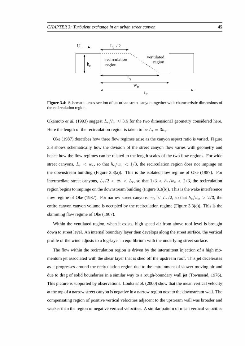
CHAPTER 3: Turbulent exchange in an urban street canyon 45
r
L
L / 2
w
h
r
recirculation
regionregion
U
e
e
e
r
ventilated
Figure 3.4: Schematic cross-section of an urban street canyon togetherwith characteristic dimensions ofthe recirculation region.
Okamotoet al. (1993) suggestLr/he ≈ 3.5 for the two dimensional geometry considered here.
Here the length of the recirculation region is taken to beLr = 3he.
Oke (1987) describes how three flow regimes arise as the canyon aspect ratio is varied. Figure
3.3 shows schematically how the division of the street canyon flow varies with geometry and
hence how the flow regimes can be related to the length scales of the two flow regions. For wide
street canyons,Lr < we, so thathe/we < 1/3, the recirculation region does not impinge on
the downstream building (Figure 3.3(a)). This is the isolated flow regime of Oke (1987). For
intermediate street canyons,Lr/2 < we < Lr, so that1/3 < he/we < 2/3, the recirculation
region begins to impinge on the downstream building (Figure3.3(b)). This is the wake interference
flow regime of Oke (1987). For narrow street canyons,we < Lr/2, so thathe/we > 2/3, the
entire canyon canyon volume is occupied by the recirculation regime (Figure 3.3(c)). This is the
skimming flow regime of Oke (1987).
Within the ventilated region, when it exists, high speed airfrom above roof level is brought
down to street level. An internal boundary layer then develops along the street surface, the vertical
profile of the wind adjusts to a log-layer in equilibrium withthe underlying street surface.
The flow within the recirculation region is driven by the intermittent injection of a high mo-
mentum jet associated with the shear layer that is shed off the upstream roof. This jet decelerates
as it progresses around the recirculation region due to the entrainment of slower moving air and
due to drag of solid boundaries in a similar way to a rough-boundary wall jet (Townsend, 1976).
This picture is supported by observations. Loukaet al.(2000) show that the mean vertical velocity
at the top of a narrow street canyon is negative in a narrow region next to the downstream wall. The
compensating region of positive vertical velocities adjacent to the upstream wall was broader and
weaker than the region of negative vertical velocities. A similar pattern of mean vertical velocities

CHAPTER 3: Turbulent exchange in an urban street canyon 46
at canyon mid-height was found by Catonet al. (2003) in observations of street canyon flow in a
water flume. Brownet al.(2000) show that turbulent intensity varies monotonicallyacross a street
canyon with low values adjacent to the upstream wall and highvalues adjacent to the downstream
walls. Finally, Barlowet al. (2004) showed that the facet averaged turbulent flux from thedown-
stream wall facet of an urban canyon was, on average, a factorof 2.2 higher than that from the
upstream wall facet. All features are consistent with a decelerating wall jet. The strength of the
flow within the recirculation region therefore depends on the path length of the jet which in turn
depends on the dimensions of the recirculation region. These arguments explain why wind speeds
decrease as the jet circulates from the downstream wall across the street, and then up the upstream
wall.
At high canyon aspect ratios, the jet may not reach the streetsurface. Numerical simula-
tions suggest that weak counter-rotating vortices may thenform in the lowest portion of the street
canyon (e.g. Siniet al., 1996; Baiket al., 2000). Hence the wind speeds, and turbulent fluxes,
deep in the canyon will be reduced in this flow regime. The effects of these complex processes on
the surface fluxes are modelled here by increasing the deceleration of the jet at these high canyon
aspect ratios.
3.5 Resistance network for an urban street canyon
The previous section described a partitioning of the canyonair flow into recirculating air and
ventilated air. This partitioning leads to three pathways for the turbulent transport from the surface
to the boundary layer above. These pathways are, firstly, from the wall and street surfaces within
the recirculation region to the recirculating air and then aloft, secondly, from the wall and street
surface within the ventilation region to the ventilated airand then aloft, and finally, from the roof
facet to the air aloft. The ventilated air and recirculatingair are each assumed to be independently
well mixed and so scalarX takes a single, but different, value within each of these twoair volumes
(Nakamura and Oke, 1988). Figure 3.5 shows the resistance network that is used to represent
transport from the facets of an urban surface to the inertialsub-layer along these three pathways.
Flux balances may now be formed for each of the pathways, as follows. LetFi denote the flux
per unit area of scalarX across theith resistor in Figure 3.5. The flux from the upstream wall and
the portion of the street that lies in the recirculation region into the recirculating air (denoted point
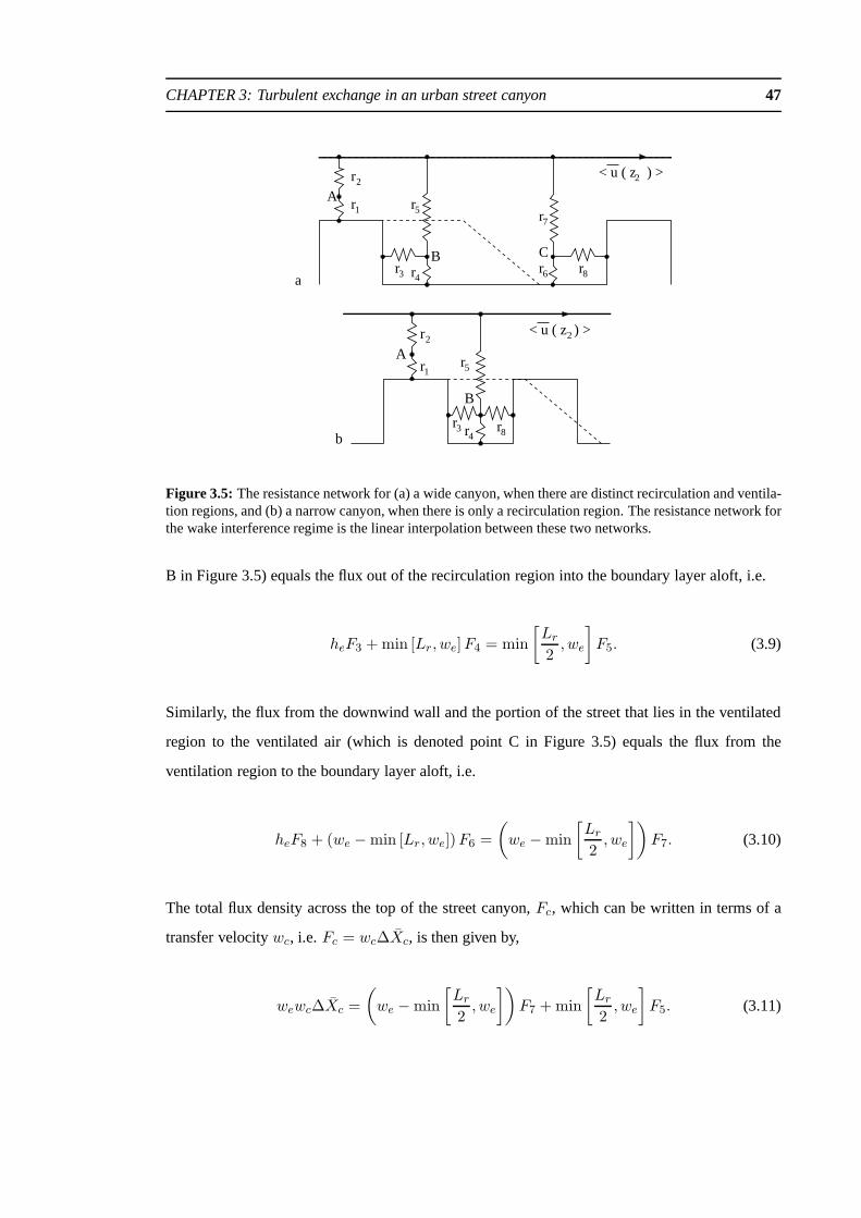
CHAPTER 3: Turbulent exchange in an urban street canyon 47
r
rrr 8
r
4r3
r
r
2
1 5
6
7
2< u ( z ) >
C
.
B
A
a
r r
r3 r4 r
1
2
5
< u ( z ) >
8
2rA
b
B
Figure 3.5: The resistance network for (a) a wide canyon, when there are distinct recirculation and ventila-tion regions, and (b) a narrow canyon, when there is only a recirculation region. The resistance network forthe wake interference regime is the linear interpolation between these two networks.
B in Figure 3.5) equals the flux out of the recirculation region into the boundary layer aloft, i.e.
heF3 + min [Lr, we]F4 = min
[
Lr
2, we
]
F5. (3.9)
Similarly, the flux from the downwind wall and the portion of the street that lies in the ventilated
region to the ventilated air (which is denoted point C in Figure 3.5) equals the flux from the
ventilation region to the boundary layer aloft, i.e.
heF8 + (we − min [Lr, we])F6 =
(
we − min
[
Lr
2, we
])
F7. (3.10)
The total flux density across the top of the street canyon,Fc, which can be written in terms of a
transfer velocitywc, i.e.Fc = wc∆Xc, is then given by,
wewc∆Xc =
(
we − min
[
Lr
2, we
])
F7 + min
[
Lr
2, we
]
F5. (3.11)
CHAPTER 3: Turbulent exchange in an urban street canyon 48
Similarly the flux density from the roof,Fr = wr∆Xr, is given by
(re − we)wr∆Xr = (re − we)F2 = (re − we)F1. (3.12)
Finally the total flux density from the street canyon,Ft = wt∆Xt, is given by
rewt∆Xt = reFt = (re − we)F2 + min
[
Lr
2, we
]
F5 +
(
we − min
[
Lr
2, we
])
F7. (3.13)
The use of the minima ofLr andW orLr/2 andW in Equations (3.9)–(3.13) arises as the dimen-
sions of the recirculating region cannot exceed those of thecanyon cavity itself.∆X in Equations
(3.11)–(3.13) represents the difference between the valueX takes at the surface, averaged over the
surface area of the individual facets concerned, and the valueX takes at the atmospheric reference
level, z2. This formulation shows how the valueX takes at one facet can influence the flux from
the other facets by changing the value ofX at the intermediate points A, B and C.
The values of the resistances in the network shown in Figure 3.5 fall into either of two generic
types. The resistance to transport from each facet to the intermediate points A, B or C in the
figure is determined by that across the internal boundary layers that develop along each facet.
The resistance to transport between the intermediate points A, B or C and the reference heightz2
represents the resistance to transport across a free shear layer. Section 3.2 developed the formulae
for the resistance to transport across an internal boundarylayer (Equation (3.5)) and across a free
shear layer (Equation (3.7)).
Section 3.2 formulates each of the resistances to transportin terms of the local wind speeds.
Therefore all that remains is the specification of wind speeds to parameterise each of the fluxes
Fi in Equations (3.9)–(3.13). Figure 3.6 shows the location and nomenclature used for these
representative winds. The geometric dependence of the forcing wind speed〈u(z2)〉 and these
representative wind speeds is considered next.
3.5.1 Wind profile in the inertial sub-layer
The vertical profile of the wind in the inertial sub-layer of the atmospheric boundary layer is
characterised by a roughness length and displacement height for the underlying urban surface,

CHAPTER 3: Turbulent exchange in an urban street canyon 49
rf
uw
ct
us
U
re
dw
dsUU
rf UU
UU
U
< u (z ) >2
Figure 3.6: Schematic of the representative winds and their positions.
namely
〈u(z)〉 =u∗κ
ln
(
z − dT
z0T
)
, (3.14)
whereκ is the von Karman constant taking a value of 0.4 andu∗ = (τ/ρ)1/2 is the friction velocity.
The dependence of the flow in the inertial sub-layer on the characteristics of the urban area can
be represented by abulk or effective roughness length, z0T
, andeffective displacement height, dT
(Grimmond and Oke, 1999a). Macdonaldet al. (1998) calculate the vertically integrated drag on
an array of cubes and deduce analytical forms for the roughness length and displacement height
as functions of the morphological characteristics of the surface. These expressions have many of
the observed features of urban roughness lengths and displacement heights (Grimmond and Oke,
1999a). These functions are used here with the morphological characteristics appropriate for two
dimensional street canyons, namely
dT
he= 1 −
we
reA−(1−we/re), (3.15)
z0T
he=
(
1 −d
T
he
)
exp
−
(
CD
κ2
(
1 −d
T
he
)
he
we
we
re
)−1/2
, (3.16)
whereCD ' 1.2 is the drag coefficient relating to the mean wind at canyon topandA ' 4.43 is
an empirical constant whose value depends on the building layout.
Figure 3.7 shows the effective roughness length and effective displacement height, normalized
by the building height, for a series of street canyons with the buildings represented by square bars
oriented normally to the wind at varying separations. Figure 3.7 also shows the wind speed at
twice the building height normalized by the free-stream wind speed,Uδ, which is taken to be the
externally imposed forcing of the scalar transport. To facilitate comparison between the model

CHAPTER 3: Turbulent exchange in an urban street canyon 50
and observations (Section 3.6) the free-stream wind is taken at the height of the reference wind
in the wind tunnel of Barlowet al. (2004), i.e.zδ = 9.5he. Note how, as the canyon aspect ratio
increases, there is a rapid drop and subsequent slow rise in the wind speed atz2 = 2he due to the
combined effects of roughness and displacement.
0.00.1 0.2 0.3 0.4 0.5 0.6 0.7
λf
0 0.5 1 1.5 2 2.50
0.2
0.4
0.6
0.8
1
canyon aspect ratio - he / w
e
Figure 3.7: Normalized effective parameters for the vertical profile ofthe mean wind in the inertial sub-layer over a sequence of street canyons calculated using themethod of Macdonaldet al., (1998). Solid line,roughness length for momentum,z
0T/he; dashed-dotted line, displacement height of flow,d
T/he; dashed
line, wind speed at twice building height normalized by the free stream flow,〈u(z2)〉/Uδ.
Cheng and Castro (2002) observe in wind tunnel studies over an urban-type roughness that
when the vertical wind profile is spatially averaged the log-layer observed in the inertial sub-layer
extends right down to roof level. The wind speed at the reference level,z2 = 2he, and wind speed
at canyon top,uct, are then,
〈u(z2)〉 =u∗κ
ln
(
2he − dT
z0T
)
, (3.17)
uct
Uδ= ln
(
he − dT
z0T
)/
ln
(
zδ − dT
z0T
)
. (3.18)
This variation of wind speed at canyon top with geometry exerts one of the strong controls on
scalar transport from the surface (Section 3.6).
CHAPTER 3: Turbulent exchange in an urban street canyon 51
3.5.2 Transport from the roof
The resistance to transport from the roof, and indeed each facet, to the intermediate point A repre-
sents the resistance to transport across the internal boundary layer that develops along its length.
Since the depth of the internal boundary layer grows as the length of the roof facet increases, it
follows that the resistances increase with facet length. For simplicity, the depth of the internal
boundary layer is taken to be 10% of the facet length.
As for the wind speed at canyon top the representative wind speed for the roof facet,urf , is
obtained by extrapolating the wind profile in the inertial sub-layer down to the depth of the internal
boundary layer along the roof facet, namely
urf
〈u(z2)〉= ln
(
he + δrf − dT
z0T
)/
ln
(
z2 − dT
z0T
)
. (3.19)
The resistance to transport from the roof facet to this point, A in Figure 3.5, is then given using
Equation (3.5) and the resistance from A to the air aloft using Equation (3.7), which yield
r1 = ln
(
δrfz
0m
)
ln
(
δrfz
0X
)
/
κ2urf , (3.20)
r2 =〈u(z2)〉 − urf
u2∗
, (3.21)
wherez0m andz
0Xare the roughness lengths for momentum andX respectively for the surface
material of the roof facet, andu∗ is calculated from the wind profile in the inertial sub-layer.
Finally δrf is the thickness of the internal boundary layer developed along the roof facet, taken as
δrf = min[0.1(re − we), z2 − he].
3.5.3 Transport from the recirculation region
The measurements of Barlowet al. (2004) and the fluid dynamical ideas developed in Section
3.4 motivated a description of the flow in the recirculation region as that of a jet that decelerates
as it travels around the canyon. Balancing advection,u∂u/∂x, and turbulent drag,τ ∼ cDu2
in the jet, yields a flow speed in the jet that decelerates exponentially with distance. There are a
number of more sophisticated theoretical descriptions of the deceleration and entrainment of a jet

CHAPTER 3: Turbulent exchange in an urban street canyon 52
on a flat wall, (e.g. Townsend, 1976; Hogget al., 1997). However, the jet within the street canyon
turns corners as it circulates within the canyon and so this work is not immediately applicable.
Additionally, these more detailed models add further parameters to the formulation of the flow
with no method of determining their value or their geometricdependence. Here, therefore, the
simple exponential description is used.
First consider the wind speed of the jet when it first impingeson the street facet,ure. This
wind speed is then the wind speed at canyon top,uct, scaled down exponentially to account for
entrainment, i.e.
ure = uct exp −α1Lse/he , (3.22)
whereLse is the length of the sloping edge of the recirculation region. The strongest flow and
highest turbulent intensity along the canyon facets is thenlocated at the end of the recirculation
region as observed by Okamotoet al. (1993).
The jet then circulates along the street and wall facets in the recirculation region, and the wind
speed varies as
u(x) = ure exp −α2x/he , (3.23)
wherex is the total distance travelled by the jet from the end of the recirculation region. The two
exponentsα1 andα2 are different due to the different physical processes whichthey represent.
The wind speeds representative of the turbulent flux from theupstream wall,uuw, from the
fraction of the street facet in the recirculation region,uus, and from the downstream wall if it is in
the recirculation region,udw, are taken as the average of the flowu(x) along each facet, namely
u† =ure
b
a+b∫
a
exp −α2x/hedx, (3.24)
where† is one ofuw, us or dw, the total distance travelled by the jet to the start of the facet in
question isa andb is the length of the facet. For example, when considering thetransfer from the
upstream wall, in the isolated roughness regimea = Lr andb = he, and in the skimming flow
regimea = we + he andb = he.
CHAPTER 3: Turbulent exchange in an urban street canyon 53
Internal boundary layers of a fixed depth of0.1he are then taken on each facet. The resistances
to transport,r3, r4, r5 andr8 (in the skimming flow regime) are then calculated from Equations
(3.5) and (3.7) as
r3 = ln
(
0.1he
z0m
)
ln
(
0.1he
z0X
)
/
κ2uuw, (3.25)
r4 = ln
(
0.1he
z0m
)
ln
(
0.1he
z0X
)
/
κ2uus, (3.26)
r5 =〈u(z2)〉 − uus
u2∗
, (3.27)
r8 = ln
(
0.1he
z0m
)
ln
(
0.1he
z0X
)
/
κ2udw, (3.28)
whereu∗ is the friction velocity calculated from the wind profile in the inertial sub-layer.uus
is used in Equation (3.27) and notuuw or udw as these are representative wind speeds for the
turbulent transfer in the narrow regions next to each wall whereasr5 represents the transfer across
the entire top of the recirculation region.
3.5.4 Transport from the ventilated region
Part of the jet that impinges on the street facet moves along the street facet into the ventilated
region. Within the ventilated region high momentum air is transported downwards so that the jet
is only decelerated somewhat. This mechanism is not available in the recirculation region which
therefore has lower wind speeds. The wind speeds representative of the turbulent transport from
the downstream fraction of the street,uds, and the downstream wall in the isolated roughness
regime case,udw, are given as
uds =ure
we − Lr
we−Lr∫
0
exp −α2x/hedx, (3.29)
udw =ure
he
we−Lr+he∫
we−Lr
exp −α2x/hedx. (3.30)
As before these wind speeds are taken to be located0.1he away from the facets.
CHAPTER 3: Turbulent exchange in an urban street canyon 54
As explained above, the mixing of high momentum air downwards in the ventilated region
street places prevents the turbulent transport in the ventilated region from decreasing to the extent
happening in the recirculation region. Here this process isrepresented by placing a minimum
bound on the wind speeds computed using Equation (3.29) and (3.30). These bounds are taken
from the wind profile established in an undisplaced boundarylayer in equilibrium with the under-
lying surface when forced by the wind speeduct at a heightz = he. The minimum wind speed
for uds is the value taken from this profile atz = 0.1he, namely
minuds = uct ln
(
0.1he
z0m
)
/
ln
(
he
z0m
)
. (3.31)
Similarly, the equilibrated wind profile would then be incident on the downstream wall. The
resulting turbulent transport from the wall scales as the vertical average of the wind profile. It
follows that there is a minimum bound on the wind speedudw in the isolated roughness and wake
interference flow regimes which is
minudw =uct
he − z0m
he∫
z0m
ln
(
0.1he
z0m
)
/
ln
(
he
z0m
)
dz. (3.32)
The resistances to transportr6, r7 andr8 (in the isolated roughness flow regime) are then given
as
r6 = ln
(
0.1he
z0m
)
ln
(
0.1he
z0X
)
/
κ2uds, (3.33)
r7 =〈u(z2)〉 − uds
u2∗
, (3.34)
r8 = ln
(
0.1z
z0m
)
ln
(
0.1he
z0X
)
/
κ2udw, (3.35)
whereu∗ is the friction velocity calculated from the wind profile in the inertial sub-layer.
The resistance to transportr8 in the wake interference flow regime is calculated by taking a
weighted average ofudw calculated in the two regions and then linkingr8 to both points B and C
in Figure 3.5.
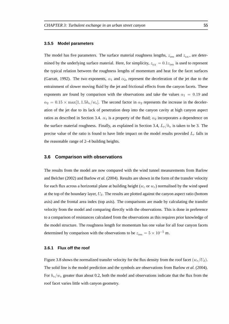
CHAPTER 3: Turbulent exchange in an urban street canyon 55
3.5.5 Model parameters
The model has five parameters. The surface material roughness lengths,z0m andz
0X, are deter-
mined by the underlying surface material. Here, for simplicity, z0X
= 0.1z0m is used to represent
the typical relation between the roughness lengths of momentum and heat for the facet surfaces
(Garratt, 1992). The two exponents,α1 andα2, represent the deceleration of the jet due to the
entrainment of slower moving fluid by the jet and frictional effects from the canyon facets. These
exponents are found by comparison with the observations andtake the valuesα1 = 0.19 and
α2 = 0.15 × max[1, 1.5he/we]. The second factor inα2 represents the increase in the deceler-
ation of the jet due to its lack of penetration deep into the canyon cavity at high canyon aspect
ratios as described in Section 3.4.α1 is a property of the fluid;α2 incorporates a dependence on
the surface material roughness. Finally, as explained in Section 3.4,Lr/he is taken to be 3. The
precise value of the ratio is found to have little impact on the model results providedLr falls in
the reasonable range of 2–4 building heights.
3.6 Comparison with observations
The results from the model are now compared with the wind tunnel measurements from Barlow
and Belcher (2002) and Barlowet al.(2004). Results are shown in the form of the transfer velocity
for each flux across a horizontal plane at building height (wc orwr) normalised by the wind speed
at the top of the boundary layer,Uδ. The results are plotted against the canyon aspect ratio (bottom
axis) and the frontal area index (top axis). The comparisonsare made by calculating the transfer
velocity from the model and comparing directly with the observations. This is done in preference
to a comparison of resistances calculated from the observations as this requires prior knowledge of
the model structure. The roughness length for momentum has one value for all four canyon facets
determined by comparison with the observations to bez0m = 5 × 10⁻⁵ m.
3.6.1 Flux off the roof
Figure 3.8 shows the normalized transfer velocity for the flux density from the roof facet(wr/Uδ).
The solid line is the model prediction and the symbols are observations from Barlowet al. (2004).
Forhe/we greater than about 0.2, both the model and observations indicate that the flux from the
roof facet varies little with canyon geometry.
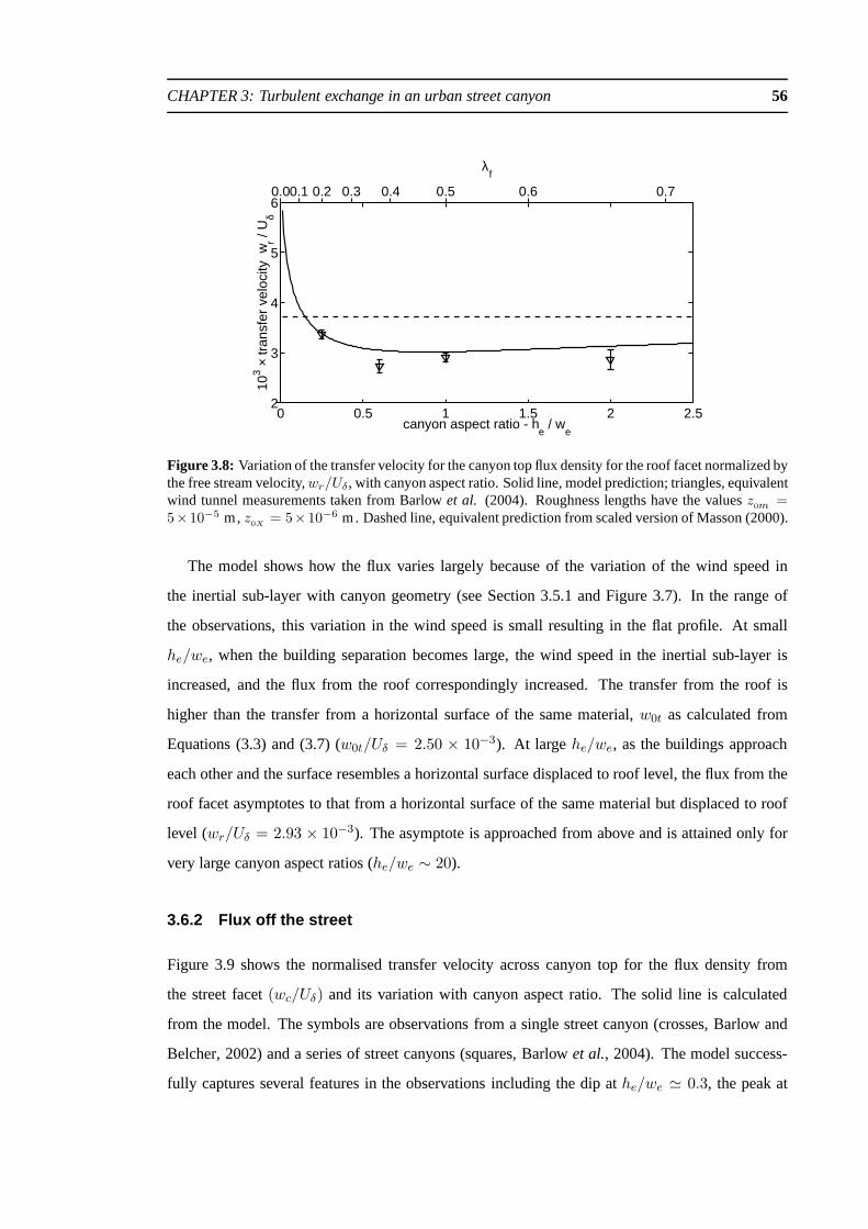
CHAPTER 3: Turbulent exchange in an urban street canyon 56
0.00.1 0.2 0.3 0.4 0.5 0.6 0.7
λf
0 0.5 1 1.5 2 2.52
3
4
5
6
canyon aspect ratio - he / w
e
103 ×
tran
sfer
vel
ocity
wr /
Uδ
Figure 3.8: Variation of the transfer velocity for the canyon top flux density for the roof facet normalized bythe free stream velocity,wr/Uδ, with canyon aspect ratio. Solid line, model prediction; triangles, equivalentwind tunnel measurements taken from Barlowet al. (2004). Roughness lengths have the valuesz
0m =5×10⁻⁵ m, z
0X= 5×10⁻⁶ m. Dashed line, equivalent prediction from scaled version of Masson (2000).
The model shows how the flux varies largely because of the variation of the wind speed in
the inertial sub-layer with canyon geometry (see Section 3.5.1 and Figure 3.7). In the range of
the observations, this variation in the wind speed is small resulting in the flat profile. At small
he/we, when the building separation becomes large, the wind speedin the inertial sub-layer is
increased, and the flux from the roof correspondingly increased. The transfer from the roof is
higher than the transfer from a horizontal surface of the same material,w0t as calculated from
Equations (3.3) and (3.7) (w0t/Uδ = 2.50 × 10⁻³). At largehe/we, as the buildings approach
each other and the surface resembles a horizontal surface displaced to roof level, the flux from the
roof facet asymptotes to that from a horizontal surface of the same material but displaced to roof
level (wr/Uδ = 2.93 × 10⁻³). The asymptote is approached from above and is attained only for
very large canyon aspect ratios (he/we ∼ 20).
3.6.2 Flux off the street
Figure 3.9 shows the normalised transfer velocity across canyon top for the flux density from
the street facet(wc/Uδ) and its variation with canyon aspect ratio. The solid line iscalculated
from the model. The symbols are observations from a single street canyon (crosses, Barlow and
Belcher, 2002) and a series of street canyons (squares, Barlow et al., 2004). The model success-
fully captures several features in the observations including the dip athe/we ' 0.3, the peak at

CHAPTER 3: Turbulent exchange in an urban street canyon 57
0.00.1 0.2 0.3 0.4 0.5 0.6 0.7
λf
0 0.5 1 1.5 2 2.50.5
1
1.5
2
2.5
3
canyon aspect ratio - he / w
e
103 ×
tran
sfer
vel
ocity
wc /
Uδ
Figure 3.9: Variation of the transfer velocity for the canyon top flux density from the street facet normalizedby the free stream velocity,wc/Uδ, with canyon aspect ratio calculated from the weighted average of theflux through the recirculation and ventilated regions. Solid line, model prediction; symbols, equivalent windtunnel measurements taken from Barlow and Belcher (2002) (crosses) and Barlowet al. (2004) (squares).Roughness lengths have the valuesz
0m = 5 × 10⁻⁵ m, z0X
= 5 × 10⁻⁶ m. Dashed line, equivalentprediction from a scaled version of Masson (2000).
he/we ' 0.6 and the almost linear decrease as the canyon aspect ratio increases further. The
transfer from the street is notably lower than from the roof facet (Figure 3.8) for all canyon aspect
ratios.
The model of the flux from the street facet has the correct limit as the canyon aspect ratio tends
to zero, namely that of a horizontal surface of the same material located atz = 0, which yields
w0t/Uδ = 2.50 × 10⁻³. The initial decrease and subsequent general increase inwc/Uδ as the
canyon aspect ratio increases from zero to 0.6 follows the variation in the wind speed in the inertial
sub-layer (shown in Figure 3.7). The flow pattern within the street canyon also influences the flux
as explained in Section 3.5. The jet within the recirculation region decelerates as it progresses
round the canyon cavity. The deceleration is particularly marked at high canyon aspect ratios,
he/we > 0.6, due to the decreased penetration of the jet into the canyon cavity. This explains the
reduction inwc/Uδ whenhe/we > 0.6.
3.6.3 Flux off the walls
Figure 3.10 shows the normalised transfer velocities across a horizontal plane at canyon top for
the flux from the two wall facets(wc/Uδ). The transfer velocities are expressed in terms of the
flux density across canyon top for ease of comparison with theflux from the street facet. This

CHAPTER 3: Turbulent exchange in an urban street canyon 58
0.00.1 0.2 0.3 0.4 0.5 0.6 0.7
λf
0 0.5 1 1.5 2 2.50
1
2
3
4
5
canyon aspect ratio - he / w
e
103 ×
tran
sfer
vel
ocity
wc /
Uδ
Figure 3.10: Variation of the transfer velocities for the canyon top flux density from the two wall facetsnormalized by the free stream velocity,wc/Uδ, with canyon aspect ratio. Lower solid line, transfer fromthe upstream wall; upper solid line, transfer from the downstream wall calculated as a weighted averageof the flux through the recirculation and ventilated regions; symbols, equivalent wind tunnel measurementsadapted from Barlowet al. (2004) for the upstream wall (stars) and downstream wall (circles). Roughnesslengths have the valuesz
0m = 5 × 10⁻⁵ m, z0X
= 5 × 10⁻⁶ m. Dashed line, equivalent prediction forboth walls from a scaled version of Masson (2000).
normalisation introduces a dependence on the relative surface areas of the walls and canyon top,
i.e. the ratiohe/we, which leads towc/Uδ being approximately proportional tohe/we.
The flux from the downstream wall is greater than the flux from the upstream wall by approxi-
mately a factor of two for all canyon aspect ratios. The difference between the two fluxes, taking
the relative surface area into account, is increased as the canyon aspect ratio increases. These two
features relate to the variation in turbulent intensity across the street canyon. The downstream
wall experiences higher wind speeds and a higher turbulent intensity than the upstream wall for
all canyon aspect ratios. The deceleration of the flow aroundthe recirculation region results in
reduced flow and hence reduced turbulent transport from the upstream wall. As for the flux from
the street facet, this deceleration is more marked as the canyon aspect ratio increases beyond
he/we ' 0.6 which increases the difference in the flux from the two walls.
3.6.4 Total flux
Figure 3.11 shows the contribution to the flux through a horizontal plane in the inertial sub-layer
from each of the canyon facets, normalised by the transfer velocity from a horizontal surface of
the same material located atz = 0, which hasw0t/Uδ = 2.50 × 10⁻³. Also shown is the transfer

CHAPTER 3: Turbulent exchange in an urban street canyon 59
0.00.1 0.2 0.3 0.4 0.5 0.6 0.7
λf
0 0.5 1 1.5 2 2.50
0.5
1
1.5
2
canyon aspect ratio - he / w
e
tran
sfer
vel
ocity
w
t / w
0t
Figure 3.11: Transfer velocities from each of the facets and the whole canyon surface normalized by thetransfer velocity from a flat surface of equivalent surface material properties and total planar area (wt/w0t).Circles, downstream wall; stars, upstream wall; crosses, street; triangles, roof; solid line; total transport.
velocity associated with the total flux from the canyon surface,wt, calculated assuming thatX
takes the same value on all facets. Hence Figure 3.11 shows how much more efficient an urban
street canyon is at releasing scalars by turbulent transport than is a flat surface.
As Equations (3.9) and (3.10) show, the flux from one canyon facet can influence the flux
from another facet. This is achieved by altering the value ofthe scalarX in the recirculation or
ventilated regions. When there is more than one source of thescalar, the transfer velocity for the
total flux from the canyon,wc, is therefore calculated through the resistance network and is not a
simple addition of the single facet transfer velocities. For example, consider the skimming flow
regime; the value of the scalar in the canyon cavity can be found through the resistance network
as
weXc −X2
r5= we
Xst −Xc
r4+ he
Xuw −Xc
r3+ he
Xdw −Xc
r8, (3.36)
⇒ Xc =
[
we
(
Xst
r4+X2
r5
)
+ he
(
Xuw
r3+Xdw
r8
)]/[
we
r4+we
r5+he
r3+he
r8
]
. (3.37)
Hence, assuming thatX takes the same valueXs on all facets, the transfer velocitywc can be

CHAPTER 3: Turbulent exchange in an urban street canyon 60
found as
Fc = wc (Xs −X2) , (3.38)
⇒ wc =1
r5
[
we1
r4+ he
(
1
r3+
1
r8
)]/[
we
(
1
r4+
1
r5
)
+ he
(
1
r3+
1
r8
)]
. (3.39)
wt is then the average ofwc andwr weighted by the surface area at canyon top through which
each of the flux densities passes.
It is important to note that while the model performs well when compared to observations
from a single-facet source of the scalar this does not guarentee similar success when considering
sources from more than one facet. This is again because the fluxes can interact. Agreement then
relies not only on the total resistance to transport being correct, but also the partitioning of the
total resistance to transport between the individual resistances being correct. This remains a topic
for future research.
Figure 3.11 shows that the flux from each individual facet is smaller than that off a horizontal
surface for almost all canyon aspect ratios (the transfer from the roof asymptotes' 1.2). The
reason is that the canyon geometry reduces the near-surfaceflow, turbulent intensity and hence
the flux. The total flux is however greater than from a horizontal surface. This increase is due to
the increased surface area, indicated by the approximatelylinear increase in the total flux as the
canyon aspect ratio increases from zero to abouthe/we = 0.75. At high canyon aspect ratios,
he/we > 0.75, the reduction in the near-surface flow is sufficient to reduce the increase in the
total flux with total surface area.
Figures 3.8–3.10 also show values for the normalized transfer velocities calculated using the
model of Masson (2000) with a building height of 10 m (dashed lines). The order of magnitude
from the two models agree due to the similarity in the values common parameters take. The model
presented here accounts for the additional physical processes of the variation of the wind speed in
the inertial sub-layer as the geometry varies and the systematic variation in the flow field within
the street canyon. Only when these processes are accounted for do the the model predictions show
the variation with geometry found in the observations.

CHAPTER 3: Turbulent exchange in an urban street canyon 61
0.00.1 0.2 0.3 0.4 0.5 0.6 0.7
λf
0 0.5 1 1.5 2 2.510
-7
10-6
10-5
10-4
10-3
10-2
10-1
100
canyon aspect ratio - he / w
e
roug
hnes
s le
ngth
s -
z # T
/ h e
Figure 3.12: Bulk roughness lengths for momentum (solid line) (Macdonald, 1998) and scalarX (dashedline) normalised on the building heighthe for a series of square bar street canyons. Note the log-scale.
3.7 Roughness lengths for scalars
The bulk roughness length for momentum for an urban area,z0T
, represents the combined effects
of the building array on the mean wind speed and Reynolds stresses in the inertial sub-layer. In
an analogous way, thebulk or effective roughness length for a scalar, zXT , would represent the
combined effects of the buildings on the mean profile and flux of scalarX in the inertial sub-
layer. As the flow field experiences form drag in addition to the viscous and turbulent stresses over
rough surfaces, unlike the scalar field, these two roughnesslengths vary differently with surface
morphology (Roth, 2000). Within numerical weather prediction models, the effects of complex
surfaces such as orography are commonly parameterized through the use of effective roughness
lengths (e.g. Wood and Mason, 1991; Hewer and Wood, 1998). The bulk roughness length for
a scalar is defined by analogy to the transfer from a flat but displaced surface (Equation (3.5), or
Hewer and Wood, 1998). The value taken byzXT gives the same area-averaged scalar flux for a
given mean surface to air difference, namely
zXT = (z2 − dT )/
exp
κ2〈u(z2)〉
ln ((z2 − dT) /z
0T)wt
(3.40)
wherez2 is the reference level in the inertial sub-layer andwt is the transfer velocity for the total
flux.

CHAPTER 3: Turbulent exchange in an urban street canyon 62
0.00.1 0.2 0.3 0.4 0.5 0.6 0.7
λf
0 0.5 1 1.5 2 2.50
2
4
6
8
10
12
14
canyon aspect ratio - he / w
e
ln (
z 0T /
z XT )
= k
B-1
Figure 3.13: Ratio of the bulk roughness lengths for a series of urban street canyons expressed on a logscale -kB−1.
Figure 3.12 shows the bulk roughness lengths for momentum and scalar transport for a series
of urban street canyons as inferred from the model. At low canyon aspect ratios the bulk rough-
ness length for momentum is greatly increased (Figure 3.7) whereas the total flux of the scalar
is increased only slightly (Figure 3.11) from the flat surface values. The bulk roughness length
for the scalarX is therefore greatly reduced. As the canyon aspect ratio increases the total flux
remains relatively constant (Figure 3.11) and the bulk roughness length for momentum decreases
due to the transition into skimming flow (Figure 3.7). The bulk roughness length for scalar trans-
port correspondingly increases and at high canyon aspect ratios,he/we > 2, exceeds that for the
flat surface.
The ratio of the bulk roughness lengths for momentum and heat, expressed on a log-scale(
ln(z0T/z
XT) = kB−1
)
is used to describe the relative efficiencies of momentum andscalar trans-
port for different surfaces. Over bare soil and vegetated surfaces this ratio takes a value of around
2 (Garratt, 1992). Verhoefet al. (1997) showed that over sparsely vegetated surfaces this ratio
can increase up to a value of 7. Synchronous observations of the sensible heat flux and Reynolds
stresses over Vancouver, Canada (λf ≈ 0.2, Voogt and Grimmond, 2000) indicate that this ratio
takes a larger value in the range of 13–27 over an urban area. Similarly, Sugawaraet al. (2003)
observed values ofkB−1 of between 6–30 over Tokyo. These values are influenced by thetime of
day and the method used to determine the ‘surface’ temperature (Voogt and Grimmond, 2000).
Figure 3.13 shows the ratiokB−1 as calculated from the model for the range of surface mor-
phologies considered. For canyon aspect ratios of less than0.5 the model values lie within, but

CHAPTER 3: Turbulent exchange in an urban street canyon 63
at the low end, of the range of observations of Voogt and Grimmond (2000) and Sugawaraet al.
(2003). However, for higher canyon aspect ratioskB−1 falls below outside the range of the ob-
servations. There is currently insufficient observationaldata across the range of urban surface
morphologies to determine whether the model prediction is correct. However, there are two rea-
sons why the reduction inkB−1 for high canyon aspect ratios may not apply to real urban areas.
Firstly, the bulk roughness length for real urban areas is unlikely to decrease as much as Mac-
donaldet al. (1998) predict due to variability in the building height andthe variety of roof shapes
(Macdonald, pers. commun.). Accounting for this would increase the ratiokB−1 particularly for
the higher canyon aspect ratios. Secondly, the full scale observations incorporate spatially varying
surface values of the scalar and stability effects on the turbulent transport. Little is known about
how either process impacts on the scalar flux or on how these processes are influenced by surface
morphology. This issue is one example of doubts over the applicability of applying results from
wind tunnel studies, under neutral conditions within generic units of the urban surface, to real
urban areas.
3.8 Sensitivity to surface morphology
Urban area comprise building morphologies other than street canyons comprised of square bar
buildings. Figures 3.14 and 3.15 show the sensitivity of themodel to varyinghe/we andwe/re
separately with the other parameter held constant. In both cases the transfer velocities across a
plane at canyon top, normalised by the flat surface value, reflect the same processes as Figure
3.11. In each case the total flux remains above the value of a flat surface due to the increase in
total surface area. In all cases except for the flux from the roof in the case of wide roofs and narrow
street canyons (left hand side of Figure 3.15), the fluxes from the individual facets are less than
that of a flat surface. The exception highlighted above results from the form of the bulk roughness
length and displacement height which for the particular geometries concerned gives a displaced
but unroughened flow and therefore increased transport. This illustrates again the balance between
the reduction in the near surface flow, and hence reduced flux densities, and the increase in the total
surface area, which increases the total flux.
A noticeable feature is that the observed features of the turbulent transport from the street,
namely the dip and peak in the transport, are not found when varying the canyon aspect ratio on
its own. This implies thatwe/re is a key parameter when determining the turbulent fluxes froman

CHAPTER 3: Turbulent exchange in an urban street canyon 64
0 0.5 1 1.5 2 2.50
0.5
1
1.5
2
canyon aspect ratio - he / w
e
tran
sfer
vel
ocity
- w
t / w
0t
Figure 3.14: Transfer velocities from each of the facets and the whole canyon surface normalized by thetransfer velocity from a flat surface of equivalent surface material properties and total planar area (wt/w0t)while varying the canyon aspect ratio withwe/re = 0.5. Circles, downstream wall; stars, upstream wall;crosses, street; triangles, roof; solid line; total transport.
urban area and attention should be paid in determining a representative value for this parameter as
well as for the canyon aspect ratio in real cities.
3.9 Summary and conclusions
Barlow and Belcher (2002) and Barlowet al. (2004) showed that the flux of a passive scalar from
an urban street canyon under transverse flow depends on the geometry of the canyon. The variation
with canyon geometry is as much as 50% and importantly differs for each facet of the canyon. This
variation is sufficient to warrant inclusion in models of theurban surface energy balance.
The model developed here is based on a partitioning of the canyon air into two distinct regions
namely a recirculation region and a ventilated region. The partitioning ensures the correct limit for
the transfer velocities as the canyon aspect ratio becomes very small or very large. The individual
facets of the canyon flux different amounts implying the needfor different representative wind
speeds. A single canyon wind speed is unable to reproduce thegeometric dependence of all of the
facets.
It is shown that there are two principal effects of urban morphology on the flux of a passive
scalar from the surface. Firstly, canyon geometry acts to reduce the flow in the inertial sub-layer
and hence the wind speeds within the vicinity of the street canyon. This reduction in the wind
speed reduces the flux densities from the canyon facets. Secondly, the total surface area of a street

CHAPTER 3: Turbulent exchange in an urban street canyon 65
0 0.2 0.4 0.6 0.8 10
0.5
1
1.5
2
we / r
e
tran
sfer
vel
ocity
- w
t / w
0t
Figure 3.15: Transfer velocities from each of the facets and the whole canyon surface normalized by thetransfer velocity from a flat surface of equivalent surface material properties and total planar area (wt/w0t)while varyingwe/re with the canyon aspect ratio held constant at 1.0. Circles, downstream wall; stars,upstream wall; crosses, street; triangles, roof; solid line; total transport.
canyon is increased compared to a flat surface which acts to increase the total flux from the surface.
These two processes occur regardless of the specific morphology used to represent the urban area.
The model also accounts for streets and buildings made from different materials through the
roughness lengths of the underlying surface material. The transfer velocities from the model de-
pend on the ratiosz0m/he andz
0X/he. Increasing either roughness length increases the turbulent
transport and increases the magnitude of the peak in the transfer from the street facet. The rough-
ness of one facet can also influence the transfer from the other facets. Increasing the roughness
length for momentum of the street facet by a factor of ten to simulate the presence of trees, for
instance, increases the transfer from the two walls by 0–5%.
The urban street canyon is only one generic unit of an urban area. Other generic units will
have differing low level flow and turbulence fields. The modelpresented can be extended to other
generic arrays of buildings provided the wind speeds representative of the turbulent transfer are
adapted to include the appropriate physical processes occurring such as corner vortices or flow
separation due to peaked roofs. Such a generalisation remains a task for future work. The sensi-
tivity of the model to urban canyon geometry indicated that the full morphology of the urban area
is important in determining the turbulent flux of a scalar from an urban area. Different morpho-
logical dependencies arise as the building morphology is varied in different ways with the balance
between the reduced near surface flow and increase in total surface area determining the total flux.

CHAPTER 3: Turbulent exchange in an urban street canyon 66
The sensible heat flux is a key term in the surface energy balance. The present work shows how
the flux of a scalar, such as sensible heat, varies with surface geometry, albeit in neutral conditions.
It is suggested that a model for the urban energy balance thatis valid over the full range of urban
areas will need to account for this variation.

CHAPTER FOUR
Energy balance and boundary layer interactions
Urban areas impose a range of effects on the energy balance and the boundary layer potential
temperature profile. The previous chapters considered the effects of surface morphology on the
individual terms of the energy balance. The extent to which the observed impacts of urban areas
on the local climate can be attributed to the combined effects of surface morphology on the surface
energy balance is not accurately known.
The most commonly studied feature of the urban climate is thenocturnal urban canopy heat
island (e.g. Oke, 1982; Arnfield, 2003). Like many features of the urban climate this commonly
has a distinct spatial pattern with a distinct edge and a coreregion of high thermal anomalies (e.g.
Oke, 1987). While in practice the magnitude of the urban canopy heat island cannot always be
correlated accurately with the local surface morphology (Barring et al., 1985), it is likely that
surface morphology does play a role in its evolution.
The surface energy balance of urban areas varies with synoptic conditions, time and position.
There are however, many common differences between the energy balance of an urban area and
the energy balance of the surrounding rural areas. The ground heat flux is commonly increased,
the latent heat flux nearly always decreased and the phase of sensible heat flux is often delayed
particularly in the transition to negative values in the early evening (e.g. Cleugh and Oke, 1986;
Grimmond and Oke, 1995; Okeet al., 1999). Urban areas can also maintain positive sensible
heat fluxes throughout the night even in synoptic conditionswhere stable boundary layers would
otherwise be formed (e.g. Okeet al., 1999). Given the range of the physical processes influencing
the urban climate and the variety of urban areas it is surprising that most urban areas show these
common traits. This therefore gives support to the idea thata common feature of urban areas, such
as surface morphology, may be the principal cause of them.
67
CHAPTER 4: Energy balance and boundary layer interactions 68
There are a range of urban energy balance models many of whichexplicitly incorporate sur-
face morphology (e.g. Arnfield, 1982, 1990; Johnsonet al., 1991; Mills, 1993; Mills and Arnfield,
1993; Sakakibara, 1996; Masson, 2000; Kusakaet al., 2001; Martilli et al., 2002). A full investi-
gation of the influence of the canyon aspect ratio on the ratesof nocturnal cooling was considered
by Johnsonet al. (1991) and Okeet al. (1991), however, their study considered the idealised case
of no turbulent heat exchange. The shape factor effect on thelongwave radiation (Chapter 2) was
shown to be the key physical process acting. Other properties such as the substrate material were
found to be of secondary importance. Mills (1993) and Mills and Arnfield (1993) considered the
effects of surface morphology on the energy balances of the individual facets and on the energy
balance at canyon top. Surface morphology was found to influence all terms of the energy balance
of the individual facets whereas little influence on the energy balance at canyon top was observed
due to interactions within the canyon cavity. Masson (2000)considered the mean annual cycle of
the energy balance of an urban street canyon for two canyon aspect ratios. Increasing the canyon
aspect ratio tended to increase the ground heat flux at the expense of the sensible heat flux. These
studies, however, considered the surface energy balance scheme when forced by the atmosphere
and did not allow the possible feedbacks between the surfaceenergy balance and boundary layer
(e.g. Brubaker and Entekhabi, 1996). Martilli (2002) considered the variation in the boundary
layer over an urban area as the mean building height was varied. The nocturnal urban boundary
layer was deeper, the lowest levels warmer and a layer above these cooler than that of a neighbour-
ing rural boundary layer. As the majority of the observed climatological features common to most
urban areas are atmospheric phenomena, the interaction between the surface and the boundary
layer must be considered when investigating these features. A detailed investigation as to which
features of the urban boundary layer can be explained by surface morphology and the identifica-
tion of the individual physical mechanisms resulting from the surface morphology that explains
them has not been done.
This chapter therefore focusses on the influence of surface morphology on the energy balance
of an urban area and on the boundary layer above. In Sections 4.1–4.3, results from Chapters 2 and
3 are used to formulate an energy balance model for an urban street canyon. This energy balance
model is then coupled to the one-dimensional boundary layermodel of Buschet al. (1976). The
energy balance model developed therefore incorporates thedetailed physical processes occurring
at the street scale but ignores variation in the surface typeon the neighbourhood scale. The urban
energy balance and boundary layer are then able to interact as if the urban area were uniform

CHAPTER 4: Energy balance and boundary layer interactions 69
and infinitely sized and allows an investigation into the impacts of surface morphology on the
equilibrated boundary layer. The idealised diurnal cycle of the energy balance and boundary layer
over an urban area is compared to that from a flat surface in Section 4.5. A detailed analysis of
the model results allows an investigation into which features of the urban climate can be attributed
to surface morphology and the precise physical mechanisms responsible. Finally, Section 4.7
considers the sensitivity of the energy balance to surface morphology and seeks to relate this to
the spatial variation of the urban modifications of the localclimate.
4.1 The surface energy balance model
The evolution of the boundary layer over any surface is determined by the surface energy balance,
and more strictly the vertical divergence of the bulk sensible heat flux. For complex surfaces such
as urban areas, there are a range of methods to calculate the surface energy balance including spa-
tial averaging (Grimmond and Oke, 2002) and considering representative points on (e.g. Johnson
et al., 1991) or averages over each part of the surface in turn (e.g.Mills, 1993; Masson, 2000;
Kusakaet al., 2001; Martilli et al., 2002). This work uses the last of these three options. For the
purposes of this work this method has two advantages. Firstly, facet-averaging is an inherent part
of the experimental work to determine the turbulent flux of a scalar from an urban street canyon
(Chapter 3) so results from this work can be applied directlyto the energy balance model. Sec-
ondly, the impacts of a range of surface morphologies can be easily investigated using this method
unlike volumetric averaging methods. The facet-averaged energy balances for the four facets of an
urban street canyon are developed incorporating the effects of surface morphology on the radiative
and turbulent fluxes identified in previous chapters. Thebulk energy balancefor an urban area is
the combination of these four energy balances.
4.1.1 The thin-layer approximation
The energy balance for a flat surface can be written as
(1 − α)(Ksf +Kdf ) + εL↓ − L↑ −G−H − LE = 0, (4.1)
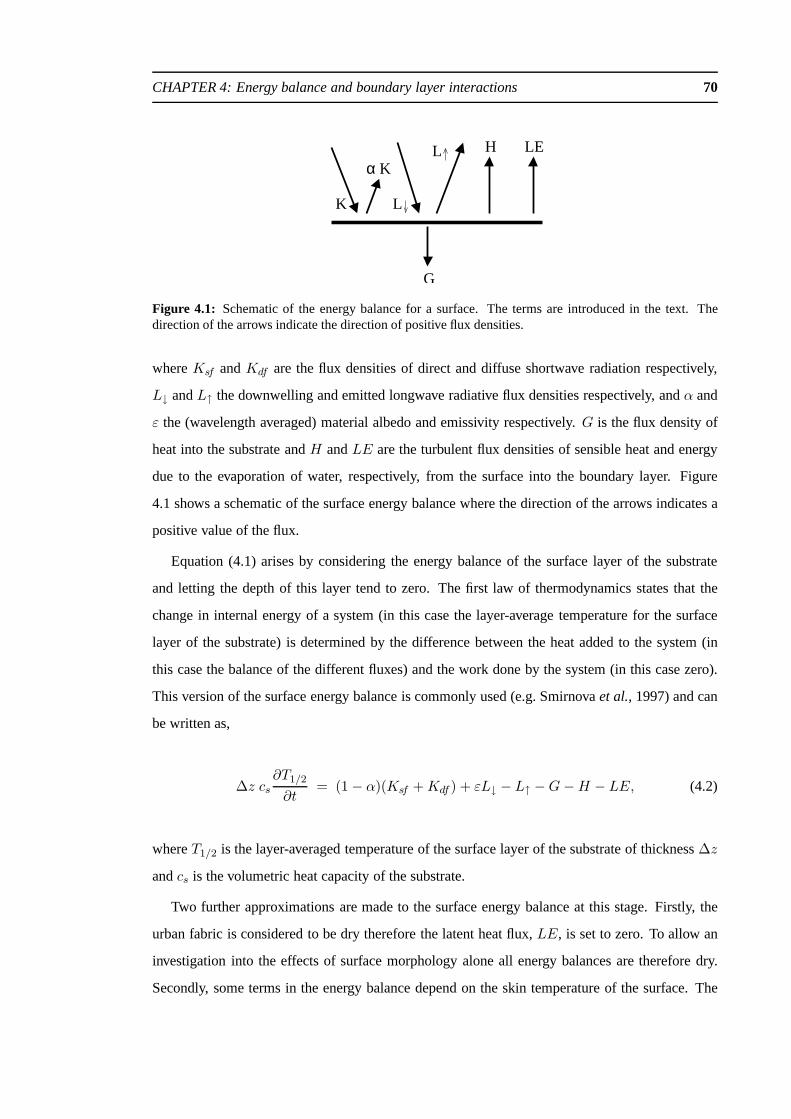
CHAPTER 4: Energy balance and boundary layer interactions 70
L
L H
G
α
K
KLE
Figure 4.1: Schematic of the energy balance for a surface. The terms are introduced in the text. Thedirection of the arrows indicate the direction of positive flux densities.
whereKsf andKdf are the flux densities of direct and diffuse shortwave radiation respectively,
L↓ andL↑ the downwelling and emitted longwave radiative flux densities respectively, andα and
ε the (wavelength averaged) material albedo and emissivity respectively.G is the flux density of
heat into the substrate andH andLE are the turbulent flux densities of sensible heat and energy
due to the evaporation of water, respectively, from the surface into the boundary layer. Figure
4.1 shows a schematic of the surface energy balance where thedirection of the arrows indicates a
positive value of the flux.
Equation (4.1) arises by considering the energy balance of the surface layer of the substrate
and letting the depth of this layer tend to zero. The first law of thermodynamics states that the
change in internal energy of a system (in this case the layer-average temperature for the surface
layer of the substrate) is determined by the difference between the heat added to the system (in
this case the balance of the different fluxes) and the work done by the system (in this case zero).
This version of the surface energy balance is commonly used (e.g. Smirnovaet al., 1997) and can
be written as,
∆z cs∂T1/2
∂t= (1 − α)(Ksf +Kdf ) + εL↓ − L↑ −G−H − LE, (4.2)
whereT1/2 is the layer-averaged temperature of the surface layer of the substrate of thickness∆z
andcs is the volumetric heat capacity of the substrate.
Two further approximations are made to the surface energy balance at this stage. Firstly, the
urban fabric is considered to be dry therefore the latent heat flux, LE, is set to zero. To allow an
investigation into the effects of surface morphology aloneall energy balances are therefore dry.
Secondly, some terms in the energy balance depend on the skintemperature of the surface. The

CHAPTER 4: Energy balance and boundary layer interactions 71
skin temperature is approximated by the layer-average temperature,T1/2, of the thin surface layer.
This approximation is justified provided the surface layer is thin so that the temperature variation
across the layer is small. If the surface layer is not thin enough that this approximation can be
made, the gradient of temperature normal to the surface should be incorporated when calculating
terms involving the skin temperature (Best, 1998b). For theresults shown here the surface layer is
5 mm or thinner for which this approximation is valid (Smirnovaet al., 1997).
4.1.2 The substrate temperature profile
To accurately calculate the ground heat flux and hence the surface temperature, the temperature
profile within the substrate is needed. The temperature profile within the substrate is governed by
the heat conduction equation, namely
G = k∂T
∂z, (4.3)
cs∂T
∂t=
∂G
∂z, (4.4)
wherek is thermal conductivity of the substrate material in WK−1m−1, cs is the volumetric heat
capacity of the substrate material in JK−1m−3 and thez-axis is positive out of the substrate (i.e.
z = 0 at the surface and decreases into the substrate).k andcs can vary within the substrate but
for the results shown here take one value each through the entire depth of the substrate.
Equations (4.3) and (4.4) require two boundary conditions as well as an initial temperature
profile. The first of the boundary conditions surface energy balance, namely
G = (1 − α)(Ksf +Kdf ) + εL↓ − L↑ −H atz = 0. (4.5)
The second boundary condition is given by either prescribing a temperature or heat flux at the
base of the calculated temperature profile i.e. prescribingeitherTin orGin in Figure 4.2. For the
flat surface energy balances used to represent ‘rural’ conditions the second boundary condition is
Gin = 0.
Equations (4.2)–(4.4) form a coupled set of equations relating the temperature profile in the
substrate to the surface energy balance. These equations are solved numerically by discretizing

CHAPTER 4: Energy balance and boundary layer interactions 72
1 2/
1 2/ ∆ z1 2/
∆ z
∆ z 1 2/1 2/
1 2/
GG
G
G
T
T
T
0
1
2
3
α
G
T
2
1
T sk
1
2
in
KK
in
LELL H
Figure 4.2: Schematic of the discretized system used to numerically solve the temperature profile withinthe substrate. Fluxes and layer-average temperatures are staggered in the vertical.
the substrate into a number of layers as shown in Figure (4.2)with the locations of the heat flux
and layer temperatures staggered. The discretized equations are then,
∆zi+1/2 cs∂Ti+1/2
∂t= Gi −Gi+1, (4.6)
Gi = kTi−1/2 − Ti+1/2
1/2(∆zi−1/2 + ∆zi+1/2), (4.7)
with Equation (4.5) giving a boundary condition onG0 and a condition onTin or Gin being the
other boundary condition.
4.1.3 The radiative and turbulent fluxes
The previous section showed how the ground heat flux and surface energy balance combine to
form a coupled set of equations for the temperature profile inthe substrate. All that remains is the
prescription of the radiative and turbulent terms in the surface energy balance.
In numerical weather prediction models the external forcing terms, i.e. the shortwave and
downwelling longwave radiative fluxes, are calculated through a complex radiative transfer model
and depend on the atmospheric temperature profile and aerosol loading. Appendix A describes the
simple model used to calculate the direct facet-averaged shortwave flux density for a plane at an
arbitrary elevation and orientation. For simplicityL↓ is taken as a constant.
The emitted longwave radiative flux density is calculated using a linearised form of the Stefan-

CHAPTER 4: Energy balance and boundary layer interactions 73
Boltzmann equation, namely
L↑ = εσT 4sk ≈ εσT 4
1/2 ' εσT 3L(4T1/2 − 3T
L), (4.8)
whereTL = 273K is a background temperature.
Finally, the turbulent sensible heat flux is formulated using the bulk aerodynamic method (Gar-
ratt, 1992; Section 3.2). Using this method the turbulent sensible heat flux is related, on dimen-
sional grounds, to the surface temperature,T1/2, and the temperature,θ(z2) at a reference level in
the inertial sub-layer,z2, namely
H = ρ cp wT(U(z2))
(
T1/2 − θ(z2))
, (4.9)
whereρ is the density of air,cp the specific heat capacity of air at constant pressure, andwT
is
the transfer velocity from the surface to the reference level. The transfer velocity is a function
of the mean wind speed at the reference level,U(z2), the surface material roughness lengths for
momentum and heat and the atmospheric stability (Section 3.2 and Appendix B).
4.2 The energy balance for an urban street canyon
The energy balance for an urban street canyon is developed from the facet-averaged energy bal-
ances and substrate temperature profiles for the four facetsof the urban street canyon. Figure (4.3)
shows a schematic of the four facet-averaged energy balances and the nomenclature used.
There are four differences between the energy balances for the urban street canyon and that of a
horizontal surface. Firstly, the second boundary condition on the ground heat flux varies between
a zero heat flux for the street facet (as that of the horizontalsurface) and a constant temperature
for the other facets. The maintenance of a constant internaltemperature acts as an anthropogenic
source of heat. Secondly, the transfer velocities,wT
, for the sensible heat flux from each facet
differ and vary with canyon geometry as described in Chapter3. Thirdly, the external radiative
forcing terms vary depending on canyon geometry (Chapter 2 and Appendix A). Finally, and the
key difference between the canyon facet energy balances andthe energy balance of a horizontal
surface is that the energy balances interact through the radiative and turbulent heat fluxes. These

CHAPTER 4: Energy balance and boundary layer interactions 74
T
T
T
cT
Τ
G
Τ
Τ
st
uw
rf
in
inin
Tdw
uw
st
w
w
w
wdw
wc
r
in
θ 2 (z )2U (z ) level of the bulk energy balance
Figure 4.3: Schematic of the facet-averaged energy balances of the urban street canyon. Separate, but in-teracting through the surface energy balances, facet-averaged substrate temperature profiles are constructedfor the roof (rf ), street (st) and both the upstream (uw) and downstream (dw) walls. The interior boundaryconditions for the roof and wall facets are a constant internal temperatureTin, that for the street facet is azero ground heat fluxGin = 0.
interaction terms are considered in the next section.
The influence of surface morphology on the energy balance of the urban street canyon can be
investigated through two sets of diagnostics. Firstly, theenergy balance and surface temperatures
for each of the facets can be considered. Secondly, thebulk energy balanceand boundary layer air
temperatures associated with the bulk energy balance can beconsidered. The bulk energy balance
is the balance of energy forms across a plane at the base of theinertial sub-layer, as marked by the
dashed line in Figure 4.3, and is the energy balance to which the boundary layer responds.
4.2.1 Interaction terms - Radiative fluxes
Chapter 2 described how geometry influences the exchange of diffuse radiation in an urban street
canyon. The matrix method developed in Chapter 2 is used for both the long and shortwave
radiative flux densities for the street and wall facets of thecanyon with the common assumptions
of diffuse reflections and uniform flux densities. To use the matrix method the surface material
albedo or emissivity and the emitted radiative fluxes must bespecified. The radiation balance for

CHAPTER 4: Energy balance and boundary layer interactions 75
the roof facet is that of a horizontal surface.
When applying the method to the shortwave radiative fluxes, the emitted flux densities from
the canyon facets are equivalent to that fraction of the direct solar radiative flux density which is
reflected. The emitted flux density for the sky facet is the diffuse radiative density. The assump-
tions of uniform radiative flux densities is unlikely to holdin practice but is in line with, and will
be of secondary importance, to the facet-averaging of the energy balances. The matrix method is
therefore applied to the shortwave radiative flux densities, using the nomenclature of Chapter 2,
with
Ωi = αiKsf i, for i = st, uw, dw, (4.10)
Ωi = Kdf i, for i = sk, (4.11)
where αsk = 0.
When applying the method to the longwave radiative fluxes, the emitted flux densities from
the canyon facets are the emitted flux densities according tothe approximated Stefan-Boltzmann
equation (Equation 4.8). The emitted flux density from the sky facet is the (diffuse) downwelling
longwave radiative flux density. The matrix method is then applied with,
Ωi = εiσT3L
(
4T1/2 i − 3TL
)
, for i = st, uw, dw, (4.12)
Ωi = L↓, for i = sk, (4.13)
where εsk = 1,
andT1/2 i is the layer-averaged temperature of the surface layer of each of theith canyon facet.
The matrix method gives that the resultant net radiative fluxdensity for each facet,Qi, can be
expressed as,
Qi =∑
i
(ψK i jΩKj + ψ
Li jΩLj) + (1 − αi)Ksf i − ΩLi, (4.14)
where the matricesψ are determined as in Chapter 2 and the subscriptsK andL denote those terms
relating to the diffuse shortwave and longwave radiation terms respectively. The energy balances
CHAPTER 4: Energy balance and boundary layer interactions 76
for the canyon facets are therefore coupled both in the external forcing, through reflections, and
directly, through the shape factor effect on the longwave radiation.
4.2.2 Interaction terms - Turbulent fluxes
Chapter 3 described how surface morphology influences the turbulent exchange of a scalar, such
as heat, from the surfaces of an urban street canyon. The model presented in Section 3.5 is used
to determine the facet-averaged turbulent sensible heat flux from the individual facets with two
modifications.
Firstly, the model developed in Chapter 3 considered only flow normal to the street canyon.
Flow parallel to the street canyon is dealt with in an analogous way to the minimum bounds on the
flow in the ventilated region of a wide street canyon. The component of the wind parallel to the
canyon is extrapolated down to roof level from the referencelevel as per the component of the wind
normal to the canyon. The flow parallel to the canyon below building height is parameterized as
a log-profile determined by the surface material roughness length and the component of the wind
parallel to the canyon at roof level. The flow parallel to the canyon at street level takes the value
this parameterized flow takes at a heightz = 0.1he. The flow parallel to the canyon along the wall
facets takes the value of this parameterized flow averaged over height. The resistances to transport
are calculated using the recombined total wind speeds usingthe formulae given in Section 3.5.
Secondly, the resistances to transport from a flat surface are influenced by the stability of the
atmosphere (Dyer, 1967). This dependence will apply to the turbulent transport from an urban area
as it does rural areas. To allow for this effect the resistances to transport are scaled according to the
larger scale atmospheric stability. The resistance to transport from a flat surface with the equivalent
bulk roughness length as that of the urban street canyon has aknown dependency on atmospheric
stability (Dyer, 1967; Busingeret al., 1971; Beljaars and Holtslag, 1991). The fractional changein
this resistance to transport is calculated given the atmospheric stability (Monin-Obukhov length).
Each resistance to transport,r1–r8, is then scaled in the same way from the neutral value given
in Chapter 3. This technique is likely to simplify the effectof stability on the transport of heat
from the urban street canyon as it does not account for features such as asymmetric heating of the
canyon air. However, in an urban area the mechanical generation of turbulence generally exceeds
that of the thermal generation/suppression of turbulence so this modification is likely to be small
(Roth, 2000).

CHAPTER 4: Energy balance and boundary layer interactions 77
Barlow et al. (2004) illustrated how the turbulent flux from one facet can influence the fluxes
from other facets. This effect is present in the formulationused to determine the turbulent fluxes
of heat from the canyon facets. For instance, in Figure 4.3, the sensible heat flux density from the
street facet in this narrow street canyon is given by (dropping the subscript1/2 for convenience),
Hst = ρcpwst(U(z2)) (Tst − Tc) . (4.15)
Tc, the mean-temperature of the air in the canyon, is dependenton the sensible heat flux densities
from each of the canyon facets and therefore the surface temperatures of those facets. Conserving
turbulent fluxes in the roughness sub-layer layer (for the skimming flow case) gives,
Tc =wcθ(z2) + wstTst + he/we (wuwTuw + wdwTdw)
wc + wst + he/we (wuw + wdw). (4.16)
The four facet-averaged energy balances of the urban streetcanyon therefore interact through
the radiative and turbulent heat fluxes and must be solved as one system.
4.3 Boundary layer formulation
The energy balances developed above are coupled to a one dimensional boundary layer model
(Buschet al., 1976) to represent the full surface-boundary layer system. This allows the impacts
of urbanisation on the boundary layer to be investigated andalso allows interactions to occur be-
tween the energy balance and boundary layer (e.g. Brubaker and Entekhabi, 1996). Applying the
hydrostatic approximation and Reynolds averaging to the Navier Stokes equations under horizon-
tal homogeneous conditions gives the following prognosticequations for the mean state of the
atmospheric boundary layer.
∂u
∂t= −f (v − vg) −
1
ρ
∂
∂z
(
ρ u′w′)
, (4.17)
∂v
∂t= f (u− ug) −
1
ρ
∂
∂z
(
ρ v′w′)
, (4.18)
∂θ
∂t= −
1
ρ
∂
∂z
(
ρ θ′w′)
, (4.19)

CHAPTER 4: Energy balance and boundary layer interactions 78
where the overbar indicates the time (and spatial) average value and the prime marks the instan-
taneous departure from the mean value.ug andvg are the westerly and southerly components of
the geostrophic wind respectively. The horizontal homogeneous condition is equivalent to stating
that there has been sufficient fetch of homogeneous surface for a fully adjusted boundary layer to
exist.
The turbulent terms are parameterised using a first order closure. The turbulence terms are
related to the vertical gradients of the mean properties, namely
u′w′ = −Km∂u
∂z, (4.20)
v′w′ = −Km∂v
∂z, (4.21)
θ′w′ = −Kh∂θ
∂z. (4.22)
Km andKh are the turbulent diffusivities for momentum and heat respectively. The values the
diffusivities take are model dependent but are related to the mean wind and temperature profiles.
Appendix B gives more details of the formulation of the specific closure method used by Busch
et al. (1976).
The surface energy balance-boundary layer coupling is achieved by carefully matching the
surface values of the turbulence terms with those from the energy balance model, i.e.
θ′w′∣
∣
s= H/ρ cp, (4.23)
−(
u′w′∣
∣
2
s+ v′w′
∣
∣
2
s
)1/2= u2
∗. (4.24)
Equations (4.17)–(4.24) are solved by discretizing the atmosphere in the vertical and using the
finite difference forms of the equations. The atmospheric lowest model level is within the inertial
sub-layer and used as the representative atmospheric levelin Equations (4.9), (4.15) and (4.16).
The influence of surface morphology on the surface energy balance and boundary layer is
investigated in two stages. Firstly, a detailed investigation of an example case is done to illustrate
the coupled nature of the system and the physical causes of thermal differences. Secondly, the
sensitivity to canyon geometry is considered. Together this allows an investigation into which

CHAPTER 4: Energy balance and boundary layer interactions 79
L
T∆
L
T
K
Figure 4.4: Schematic of the initial temperature profile (solid line) and the temperature profile after onetime period (dash-dotted line) used in the analysis of the role of surface area in determining the impacts ofsurface morphology on the energy balance of an urban area.
observed features of urban areas can be explained by the influence of surface morphology on the
energy balance and its spatial variation.
4.4 The role of surface area
The morphology of urban areas imposes two properties on the surface: An increased surface area
and surface geometry, i.e.he and the ratioshe/we, we/re and combinations thereof. Knowledge
of how one property alone influence the terms of the energy balance is useful as it allows an
assessment of the relative importance of the two properties. The probable impacts of alternative
building configurations can then be estimated. Investigating the impacts of surface geometry alone
is impractical. Assessing the role of surface area alone in determining the impact of surface mor-
phology on the surface energy balance is possible however asvarying the surface area is equivalent
to varying the incoming radiative flux densities. To tackle this issue consider the simple analysis
below.
Consider an isothermal temperature profile through the atmosphere and substrate as shown
schematically in Figure 4.4; it follows that we can setTa = Tg = TL. The incidence of solar
and/or downwelling longwave radiation implies that the surface temperature will change; let the
change in surface temperature in one time period be denoted by ∆T . For the purposes of this
analysis this change in temperature is assumed to be positive. The case of a negative change in
temperature is analogous with the conclusions given then relating to the magnitude of the changes.

CHAPTER 4: Energy balance and boundary layer interactions 80
The approximate form for the surface energy balance is then (Bristow, 1987),
(1 − α)(Ksf +Kdf ) + εL↓ − εσT 3L(T
L+ 4∆T ) − ρcpwT
∆T − k∆T/∆z = 0. (4.25)
where the other symbols take their usual meaning.
Suppose that the surface area of the surface increases by a relative factor ofA but the bulk exter-
nal radiative forcing stays the same. Provided that the surface remains flat (physically impossible)
the transfer velocitywT
stays the same i.e. the value taken in neutral conditions as determined by
the wind speed and surface material roughness lengths. Denote the flux densities from the surface
whereA = 1 by subscript1, those from the surface of increased surface area by subscriptA
. The
bulk surface energy balance then becomes,
(1 − α)(Ksf +Kdf )+εL↓ −AεσT 3L(T
L+ 4∆T
A)
−AρcpwT∆T
A−Ak∆T
A/∆z = 0, (4.26)
⇒ ∆TA
=(1 − α)(Ksf +Kdf ) + εL↓ −AεσT 4
L
4AεσT 3L
+AρcpwT+Ak/∆z
=ϕ0
A− ϕ1, (4.27)
where constantsϕ0 andϕ1 are positive definite. Equation (4.27) shows that increasing the surface
area of the surface necessarily reduces the surface temperature variation.
The flux densities and bulk fluxes from the surface also changeas the surface area is increased.
The external forcing flux densities vary solely with surfacearea with the bulk fluxes staying the
same, namely
KsfA= Ksf1 /A, (4.28)
KdfA= Kdf1 /A, (4.29)
L↓A= L↓1 /A. (4.30)
The other terms of the energy balance vary as a result of the change in surface area and the change
in temperature variation. The emitted longwave radiation flux density,L↑A, and bulk flux,AL↑A
,
CHAPTER 4: Energy balance and boundary layer interactions 81
vary as,
L↑A= εσT 3
L(T
L+ 4 (ϕ0/A− ϕ1)) < L↑1, (4.31)
AL↑A= L↑1 + (A− 1)εσT 3
L(T
L− 4ϕ1) > L↑1, (4.32)
as TL− 4ϕ1 =
ρcpwTT
L+ kT
L/∆z
4εσT 3L
+ ρcpwT+ k/∆z
> 0. (4.33)
The flux density of the emitted longwave radiation thereforedecreases as the surface area is in-
creased but the bulk flux of longwave radiation is increased.
Conversely, the bulk fluxes and flux densities of the sensibleheat and ground heat vary as,
HA
= ρcpwT(ϕ0/A− ϕ1) < H1, (4.34)
AHA
= H1 − (A− 1)ρcpwTϕ1 < H1, (4.35)
GA
=k
∆z(ϕ0/A− ϕ1) < G1, (4.36)
and AGA
= G1 − (A− 1)k
∆zϕ1 < G1. (4.37)
The density and bulk values of the sensible and ground heat fluxes are all decreased by increasing
the surface area of the surface. The effect of increasing thesurface area on the energy balance is
therefore to reduce the temperature variation and to changethe partitioning of energy forms at the
surface with more energy going into emitted radiation and less into turbulent sensible and ground
heat forms. This finding will be contrasted to the findings when considering the full effects of
surface morphology in the next section.
4.5 Case study
The role of surface morphology in determining the energy balance and boundary layer profiles
is now considered in relation to a specific case study. A comparison is made between the fully
adjusted (i.e. one-dimensional column) boundary layer profiles and the bulk energy balances es-
tablished over the urban canyon surface and over two flat dry surfaces. The ‘smooth’ surface has
the same roughness length as the material roughness length of the urban fabric. The ‘roughened’

CHAPTER 4: Energy balance and boundary layer interactions 82
surface has the same roughness length as the bulk roughenss length of the urban canyon. Com-
paring the three cases isolates the effects of surface morphology on the surface and illustrates the
advantages and disadvantages of modelling an urban area as abare soil surface with an increased
roughness length (e.g. Myrup, 1969).
For the specific cases considered the surfaces are located at60N and the day is the spring
equinox. The surface material properties for the coupled systems are equal,α = 0.1, ε = 0.98,
k = 0.75WK−1m−1, cs = 1.5 × 10⁶JK−1m−3, and are representative of common building mate-
rials such as brick (Oke, 1987). The urban geometry considered is an urban street canyon where
he/we = 1, andwe/re = 0.5, oriented north-south with a building height of 10 m. The surface
material roughness length isz0m = 0.01 m, the bulk roughness length computed for this canyon
morphology isz0T
= 0.53 m (using Macdonaldet al., 1998).
The external forcing conditions are chosen to be representative of synoptic conditions con-
ducive to longwave radiative cooling - light winds and clearskies. These conditions favour large
urban-rural thermodynamic differences (Oke, 1987). The shortwave radiative forcing is described
in Appendix A. The downwelling longwave radiative flux density is constant atL↓ = 240 W m−2
chosen to minimise the drift in time of the total energy in theflat surface case. The geostrophic
wind speed is light atug = 5 m s−1 andvg = 0 m s−1 .
The models are initialised at dawn. Figure 4.5 shows the initial temperature profiles in the
atmosphere (a) and substrate (b). The atmospheric potential temperature profile is comprised of
four layers. From the surface upwards these are a surface inversion layer, a residual layer from
the previous day’s well-mixed layer, a capping inversion and finally a stable layer in the free
troposphere.
The initial conditions in the substrate are an interpolation from the surface temperature to the
interior temperature (293 K for the internal building temperature, 285 K for the horizontal surfaces
and street facet) dependent on the surface material properties. The depth of the substrate used for
the flat surfaces and the canyon facets is greater than 0.5 m, the material properties are such that
the depth of penetration of the diurnal temperature signal is approximately 0.12 m (Garratt, 1992)
hence the boundary conditions at the base of the substrate temperature profiles are expected to play
a minor role. The constant temperature condition used for the interior of the wall and roof facets
acts as an anthropogenic heat source in the case where the interior is warmer than the substrate.
However, if the substrate is warmer than the interior this condition acts as a heat sink. This is

CHAPTER 4: Energy balance and boundary layer interactions 83
unrealistic as it implies that another source of energy mustbe employed to remove the energy
from the wall or roof substrate which is not accounted for elsewhere. These initial conditions
are representative of the substrate and atmospheric profiles established after a night conducive to
radiative cooling.
a)275 280 285 290 2950
500
1000
1500
2000
2500
3000
Potential temperature (K)
heig
ht (
m)
b)275 280 285 290 295
0
0.1
0.2
0.3
0.4
0.5
Temperature (K)de
pth
(m)
Figure 4.5: The initial conditions used in the case study. (a) Potentialtemperature profile in the boundarylayer. (b) Temperature profiles used in the substrate; solidline, profile for the flat surfaces and the streetfacet; dashed line, profile for the two wall and roof facet.
The initial wind profiles are determined from the bulk roughness length, the displacement
height and the geostrophic wind speed applied at the top of the boundary layer (zi = 1 km),
namely
u(z) =
ug ln(
(z − dT)/
z0T
)
/
ln(
(zi − dT)/
z0T
)
for z2 < z < zi,
ug for z > zi,
(4.38)
and similarly for thev-component.
Results are shown for the second model day to allow for an adjustment due to unbalanced initial
conditions but to minimise the drift between the different model runs. The energy balances for the
three coupled systems, bulk and individual facets, are considered first with the accompanying
effects on the surface and atmospheric temperatures considered later.

CHAPTER 4: Energy balance and boundary layer interactions 84
4.5.1 Case study: The bulk energy balances
The first three panels of Figure 4.6 show the bulk energy balances for the three coupled systems
considered. In each case the black solid line is the net radiative flux density, the red dashed line
is the sensible heat flux density and the green dash-dotted line is the ground heat flux density
calculated as a residual.
Figure 4.6(a) shows the energy balance from the coupled energy balance-boundary layer sys-
tem with the smooth horizontal surface. The additional dotted line on this plot is the ground heat
flux density calculated from the top two substrate layers. The close match between the calculated
ground heat flux densities and the theoretically expected reduction in magnitude and phase delay
between the two (Garratt, 1992) gives confidence that this part of the energy balance is correct.
a)0 6 12 18 24
-200
-100
0
100
200
300
400
area
ave
rage
d flu
xes
(W m
-2)
local solar time (hrs)
smooth
surface
b)0 6 12 18 24
-200
-100
0
100
200
300
400
area
ave
rage
d flu
xes
(W m
-2)
local solar time (hrs)
rough
surface
c)0 6 12 18 24
-200
-100
0
100
200
300
400
area
ave
rage
d flu
xes
(W m
-2)
local solar time (hrs)
urban streetcanyon
d)0 10 20 30 40 50 60
-1
-0.5
0
0.5
1
run time (hrs)
% c
hang
e in
tota
l ene
rgy
Figure 4.6: Diurnal energy balance profiles for the second day of the casestudy. (a) Energy balance forthe smooth surface; black solid line, net radiation; red dashed line, green sensible heat flux; dash-dottedline, ground heat flux; dotted line, ground heat flux calculated from the top two layers of the discretizedsubstrate temperature profile. (b) Energy balance for the roughened surface, lines as in (a). (c) Bulk energybalance for the canyon surface, line as in (a). (d) Profiles ofthe change in the total energy within the column(substrate and atmosphere) not explained by the accumulation of energy due to the net radiation. Black solidline, street canyon case; green dash-dotted line, smooth surface case; red dashed line, roughened surfacecase.

CHAPTER 4: Energy balance and boundary layer interactions 85
The phase differences between the peak values of the three terms relates to the diurnal tempera-
ture profiles. The solar radiative flux peaks at local midday but the emitted longwave radiative flux
depends on the surface temperature and peaks after local midday. The result is a peak in the net
radiation just before local midday. During the morning, a positive sensible heat flux acts to erode
the stable boundary generated by nocturnal longwave radiative cooling. The difference between
the surface and air temperature is therefore reduced and thesensible heat flux is small. Corre-
spondingly the ground heat flux is large during the morning and reduces later as the surface-air
temperature difference increases and the sensible heat fluxincreases. The ground heat flux there-
fore peaks in mid-morning and the sensible heat flux peaks in mid-afternoon. Stability effects on
the transfer velocity,wT
in Equation (4.9), mean that the magnitude of the sensible heat flux in
stable conditions is less than that in unstable conditions for the same surface-air temperature dif-
ference. By night, therefore, the surface energy balance isprimarily a balance between the ground
heat flux and the net radiation.
Figure 4.6(b) shows the energy balance from the coupled energy balance-boundary layer sys-
tem with the horizontal surface with increased roughness. Comparing Figures 4.6(a) and 4.6(b)
shows that the principal effect of increasing the roughnessof a surface is to alter the partitioning
between the ground heat and sensible heat forms. Increasingthe surface roughness length acts
to increase the turbulent mixing and transport from a surface via the transfer velocitywT
. The
magnitude of the sensible heat flux for a given surface-air temperature difference is therefore in-
creased and the ground heat flux correspondingly decreases in magnitude. There is also a small
increase in the magnitude of the net radiation through the day. This results from the decrease in
the diurnal variation in surface temperature, and therefore the emitted longwave radiation, which
accompanies the altered sensible heat flux (see Figure 4.8(a)).
Figure 4.6(c) shows the bulk energy balance from the urban canyon. Comparing this energy
balance to the other energy balances highlights many different effects. The ground heat flux is
slightly advanced and increased in magnitude, the sensibleheat flux is decreased in magnitude and
delayed - opposite to the effects of increasing the surface roughness length. The net radiative flux
is almost identical to the two flat-surface cases despite thelarge impacts of surface morphology
on the radiative flux densities (Chapter 2). The causes of these differences relate to the increase in
surface area and surface geometry on the individual facet energy balances as considered in detail
in Section 4.5.2.
Comparing the three figures shows that the influence of surface morphology goes some way

CHAPTER 4: Energy balance and boundary layer interactions 86
to explaining the observed differences between rural and urban bulk energy balances (e.g. Cleugh
and Oke, 1986). Surface morphology acts to increase the ground heat flux and delay the sensible
heat flux while leaving the net radiation approximately the same. A horizontal surface with in-
creased roughness does not give a satisfactory approximation to the full urban canyon surface so
casts doubt on the usefulness of approximating urban areas as bare soil surfaces with increased
roughness lengths. It should be noted here that the flat surface energy balances here are not rep-
resentative of the energy balances of rural areas. The effects of moisture and plant canopies (e.g.
Wallace and Verhoef, 1996; Finnigan, 2000) will also play a role in determining the differences
between rural and urban bulk energy balances.
Figure 4.6(d) shows the change in the total energy of the soil-atmosphere column from 50 cm
depth in the substrate to 2 km in the atmosphere, accounting for absorbed and emitted radiation
at the surface, through the model runs. For a truly conservative system this change should be
zero. The green dash-dotted line represents the change in total energy from the smooth surface
system, the red dashed line that of the roughened surface system and the black solid line that of
the canyon system. The horizontal surfaces show little unexplained change in total energy which
gives confidence in the models. The total energy of the canyonsystem has a diurnal signal and a
slight drift in time. The diurnal signal results from the approximations used to calculate the total
energy in the lowest atmospheric layer. The drift in time is due to the maintenance of the internal
building temperature which represents a source of energy. For this particular case this source of
energy is equivalent to a 3–4 W m−2 anthropogenic heat source. In all cases the change in total
energy is small.
4.5.2 Case study: The facet energy balances
The bulk energy balance for the canyon surface is comprised of the facet-averaged energy balances
of the four canyon facets. Figure 4.7 shows these four energybalances; (a) is the energy balance
for the roof facet, (b) the energy balance for the street facet, (c) the energy balance for the west-
facing wall facet and (d) the energy balance for the east facing wall facet with the lines as in Figure
4.6. Unsurprisingly the energy balance of the roof facet is similar to that of the horizontal surfaces.
The principal effect of surface morphology on the energy balances of the canyon facets is the
redistribution of the solar radiation. Facet elevation andorientation, together with shadowing,
result in the spiked profiles in the net radiation profiles. The effects of reflected radiation can be
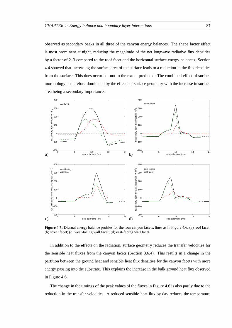
CHAPTER 4: Energy balance and boundary layer interactions 87
observed as secondary peaks in all three of the canyon energybalances. The shape factor effect
is most prominent at night, reducing the magnitude of the netlongwave radiative flux densities
by a factor of 2–3 compared to the roof facet and the horizontal surface energy balances. Section
4.4 showed that increasing the surface area of the surface leads to a reduction in the flux densities
from the surface. This does occur but not to the extent predicted. The combined effect of surface
morphology is therefore dominated by the effects of surfacegeometry with the increase in surface
area being a secondary importance.
a)0 6 12 18 24
-200
-100
0
100
200
300
400
flux
dens
ity fr
om th
e ro
of (
W m
-2)
local solar time (hrs)
roof facet
b)0 6 12 18 24
-200
-100
0
100
200
300
400
flux
dens
ity fr
om th
e st
reet
(W
m-2
)
local solar time (hrs)
street facet
c)0 6 12 18 24
-200
-100
0
100
200
300
400
flux
dens
ity fr
om th
e w
est f
acin
g w
all (
W m
-2)
local solar time (hrs)
wall facetwest facing
d)0 6 12 18 24
-200
-100
0
100
200
300
400
flux
dens
ity fr
om th
e ea
st fa
cing
wal
l (W
m-2
)
local solar time (hrs)
east facingwall facet
Figure 4.7: Diurnal energy balance profiles for the four canyon facets, lines as in Figure 4.6. (a) roof facet;(b) street facet; (c) west-facing wall facet; (d) east-facing wall facet.
In addition to the effects on the radiation, surface geometry reduces the transfer velocities for
the sensible heat fluxes from the canyon facets (Section 3.6.4). This results in a change in the
partition between the ground heat and sensible heat flux densities for the canyon facets with more
energy passing into the substrate. This explains the increase in the bulk ground heat flux observed
in Figure 4.6.
The change in the timings of the peak values of the fluxes in Figure 4.6 is also partly due to the
reduction in the transfer velocities. A reduced sensible heat flux by day reduces the temperature
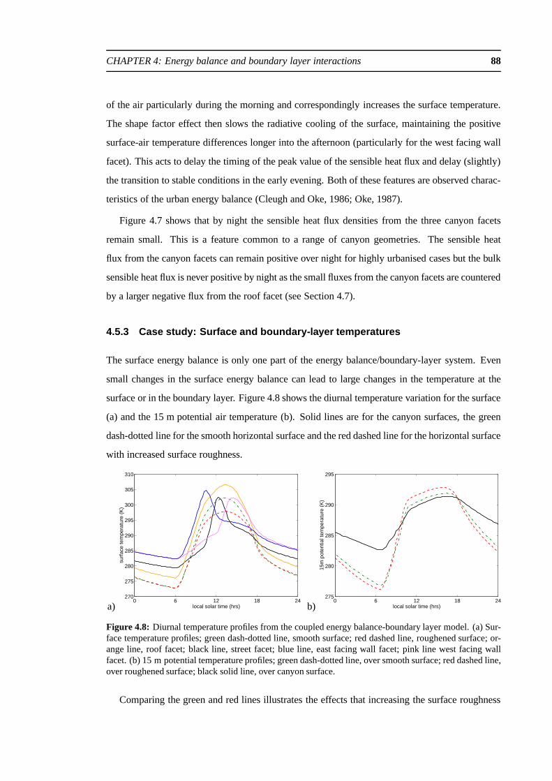
CHAPTER 4: Energy balance and boundary layer interactions 88
of the air particularly during the morning and correspondingly increases the surface temperature.
The shape factor effect then slows the radiative cooling of the surface, maintaining the positive
surface-air temperature differences longer into the afternoon (particularly for the west facing wall
facet). This acts to delay the timing of the peak value of the sensible heat flux and delay (slightly)
the transition to stable conditions in the early evening. Both of these features are observed charac-
teristics of the urban energy balance (Cleugh and Oke, 1986;Oke, 1987).
Figure 4.7 shows that by night the sensible heat flux densities from the three canyon facets
remain small. This is a feature common to a range of canyon geometries. The sensible heat
flux from the canyon facets can remain positive over night forhighly urbanised cases but the bulk
sensible heat flux is never positive by night as the small fluxes from the canyon facets are countered
by a larger negative flux from the roof facet (see Section 4.7).
4.5.3 Case study: Surface and boundary-layer temperatures
The surface energy balance is only one part of the energy balance/boundary-layer system. Even
small changes in the surface energy balance can lead to largechanges in the temperature at the
surface or in the boundary layer. Figure 4.8 shows the diurnal temperature variation for the surface
(a) and the 15 m potential air temperature (b). Solid lines are for the canyon surfaces, the green
dash-dotted line for the smooth horizontal surface and the red dashed line for the horizontal surface
with increased surface roughness.
a)0 6 12 18 24
270
275
280
285
290
295
300
305
310
local solar time (hrs)
surf
ace
tem
pera
ture
(K
)
b)0 6 12 18 24
275
280
285
290
295
local solar time (hrs)
15m
pot
entia
l tem
pera
ture
(K
)
Figure 4.8: Diurnal temperature profiles from the coupled energy balance-boundary layer model. (a) Sur-face temperature profiles; green dash-dotted line, smooth surface; red dashed line, roughened surface; or-ange line, roof facet; black line, street facet; blue line, east facing wall facet; pink line west facing wallfacet. (b) 15 m potential temperature profiles; green dash-dotted line, over smooth surface; red dashed line,over roughened surface; black solid line, over canyon surface.
Comparing the green and red lines illustrates the effects that increasing the surface roughness

CHAPTER 4: Energy balance and boundary layer interactions 89
has on the temperatures. Accompanying an increase in the magnitude of the sensible heat flux
density (Figures 4.6(a) and (b)), there is a decrease in the maximum surface temperature and a
decrease in the diurnal temperature range at 15 m. The increase in the transfer velocity due to
the increase in the surface roughness length acts to couple the surface and air temperatures more
strongly. The maximum surface temperatures achieved in unstable conditions are therefore re-
duced. By night the principal energy balance is between the ground heat flux and the net radiation
resulting in surface temperatures which are very similar. Changing the surface roughness length
acts to redistribute the energy in the column. The relative sizes of the heat capacities of the sub-
strate and atmosphere mean that a small (indistinguishable) difference in the substrate temperature
can correspond to a larger difference in the atmospheric temperature profiles at night, as seen in
Figure 4.8(b).
The solid lines in Figure 4.8(a) show the surface temperatures of the canyon facets (orange
is the roof facet, black the street facet, blue the east-facing wall facet and pink the west-facing
wall facet). The non-uniformity of the solar radiation due to the elevation and orientation of the
different facets and shadowing are again the dominant processes acting by day. There is a reduction
in the diurnal range of the surface temperatures and an offset in the mean surface temperature. The
reduction in the diurnal range of the surface temperatures is expected due to the increase in surface
area (Section 4.4). The offset in the mean temperature results from the shape factor effect on the
net radiation (Chapter 2) and the interactions between the surface and the boundary layer. The
shape factor effect acts to reduce the longwave radiative cooling of the canyon facets, particularly
at night, and gives the warmer nocturnal surface and air temperatures seen in the two figures.
For the geometry considered, the shape factor effect reduces the longwave radiative cooling of
the street facet less than that of the wall facets giving riseto the difference between the wall and
street temperatures during the night. The shape factor effect by itself cannot explain the increased
night time temperature of the roof facet when compared to thehorizontal surfaces. This increased
temperature arises due the interactions between the surface and the boundary layer. The reduced
nocturnal cooling of the canyon facets leads to a reduction in the cooling of the boundary layer
(the bulk sensible heat flux is reduced) and a reduction in atmospheric stability. This reduction in
stability acts to further increase the transfer velocity for the roof facet (wr) which is greater than
that of a flat surface (Section 3.6.1). The roof and 15 m temperatures are therefore more strongly
coupled during the night than a flat surface and the surface temperature does not cool as much
despite no radiative impacts on the net radiation.

CHAPTER 4: Energy balance and boundary layer interactions 90
Figure 4.9 shows boundary layer potential temperature profiles from the three systems con-
sidered every three hours through the day. In each figure the black solid line is the profile above
the canyon surface, the green dash-dotted line that over thesmooth horizontal surface and the red
dashed-line that over the horizontal surface with the increased surface roughness length. Only the
lowest 500 m of the boundary layer is shown as above this levelthe differences between the cases
are small.
Most of the boundary layer remains near-neutral throughoutthe day in all of the cases consid-
ered. The neutral profiles are established by deep turbulentmixing during the day and maintained
through the night as there are no radiative processes actingin the boundary layer model and the
turbulent cooling of a stable boundary layer acts only in thelowest layers. The differences between
the neutral parts of the boundary layer profiles result from the differences in the time-integrated
sensible heat flux from the three surfaces. The differences in the profiles are small since during the
day, when the differences in the surface forcing are greatest, the boundary layer is deep, extending
to over 1 km.
In a stable boundary layer, stability effects limit the depth through which turbulent mixing can
occur and the boundary layer is shallower. Any differences in the surface forcing are therefore
concentrated in this shallower layer and are likely to be of greater magnitude. The stability of
the boundary layer is determined by the surface temperature, and therefore the surface energy
balance, and the turbulent mixing within the boundary layer. The two horizontal surfaces have
approximately the same surface temperature during the night (Figure 4.8). The increase in turbu-
lent mixing due to the increased surface roughness length mixes the nocturnal cooling through a
deeper layer. Increasing the surface roughness length therefore acts to deepen and cool the stable
nocturnal boundary layer.
The large differences between the nocturnal boundary layers over the horizontal surfaces and
the canyon surface illustrate the coupled nature of the system. The surface temperatures of the
canyon facets remain warmer than those of the horizontal surfaces (Figure 4.8). With a boundary
layer that has developed with the surface through the day, this automatically results in a reduction
in the magnitude of the (negative) turbulent sensible heat flux and therefore a reduction in the
stability of the boundary layer. However, two other boundary layer processes act to reinforce the
nocturnal thermal differences between the boundary layersover the horizontal and canyon sur-
faces. Firstly, the increase in the bulk surface roughness has the same effect as before acting to
spread the cooling in the vertical. Secondly, the turbulentmixing in the boundary layer is stabil-
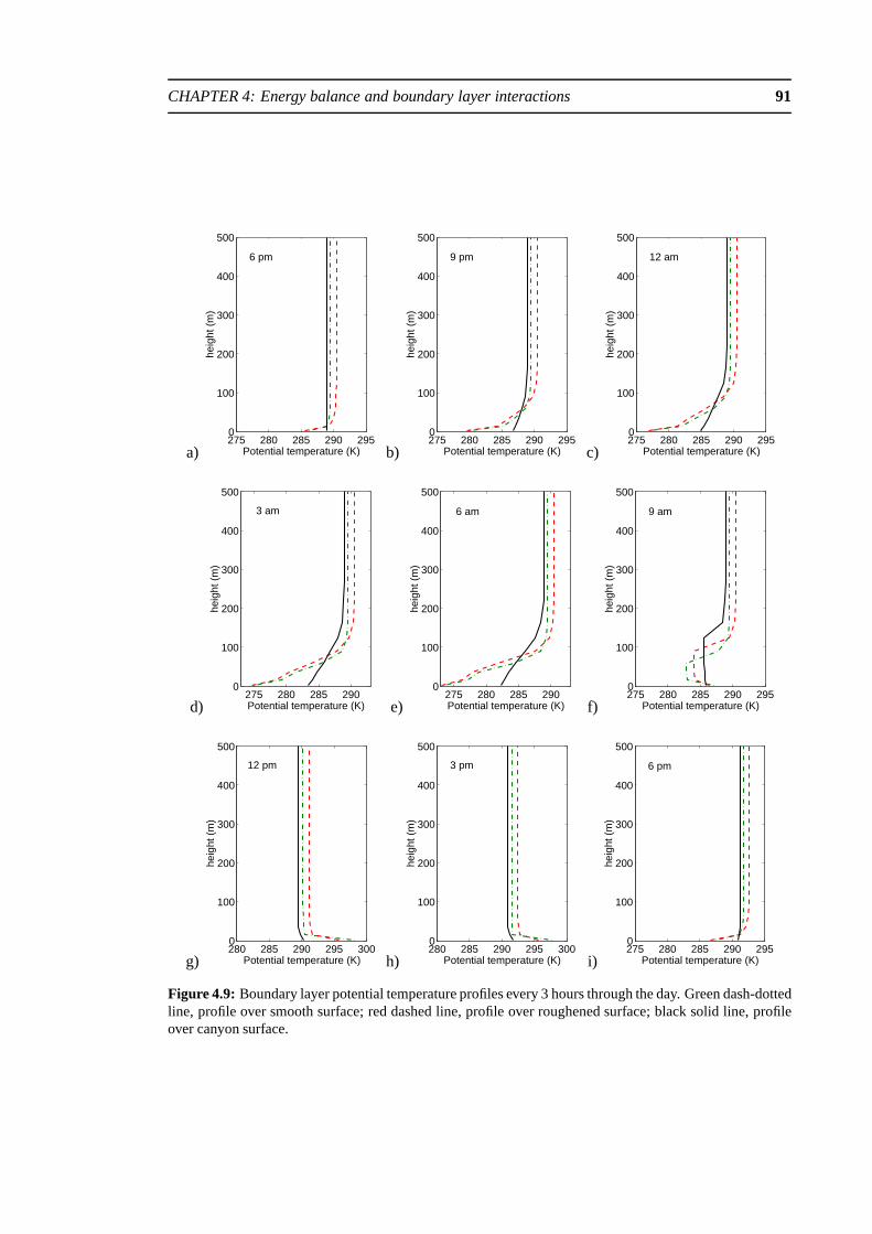
CHAPTER 4: Energy balance and boundary layer interactions 91
a)275 280 285 290 2950
100
200
300
400
500
heig
ht (
m)
Potential temperature (K)
6 pm
b)275 280 285 290 2950
100
200
300
400
500
heig
ht (
m)
Potential temperature (K)
9 pm
c)275 280 285 290 2950
100
200
300
400
500
heig
ht (
m)
Potential temperature (K)
12 am
d)275 280 285 290
0
100
200
300
400
500
heig
ht (
m)
Potential temperature (K)
3 am
e)275 280 285 290
0
100
200
300
400
500
heig
ht (
m)
Potential temperature (K)
6 am
f)275 280 285 290 2950
100
200
300
400
500
heig
ht (
m)
Potential temperature (K)
9 am
g)280 285 290 295 3000
100
200
300
400
500
heig
ht (
m)
Potential temperature (K)
12 pm
h)280 285 290 295 3000
100
200
300
400
500
heig
ht (
m)
Potential temperature (K)
3 pm
i)275 280 285 290 2950
100
200
300
400
500
heig
ht (
m)
Potential temperature (K)
6 pm
Figure 4.9: Boundary layer potential temperature profiles every 3 hoursthrough the day. Green dash-dottedline, profile over smooth surface; red dashed line, profile over roughened surface; black solid line, profileover canyon surface.

CHAPTER 4: Energy balance and boundary layer interactions 92
ity dependent. A reduction in the stability of the boundary layer increases the turbulent mixing
allowing heat from the overlying residual layer to be mixed downwards which reduces further the
stability of the boundary layer by warming the lowest layersand deepening the stable boundary
layer. The combined effects of surface morphology on the energy balance/boundary-layer system
thus results in deeper, warmer, less stable nocturnal boundary layers when compared to a bound-
ary layer over a horizontal surface. These boundary layer features are commonly observed during
heat island conditions (e.g. Oke and East, 1971).
4.5.4 Case study: Summary
The boundary layer potential temperature profile and surface energy balance are interdependent.
Differences between the potential temperature profile overdifferent surfaces relate to physical
processes acting in the energy balance, e.g. the nocturnal atmospheric temperature differences
relate primarily to the shape factor effect on the longwave radiation. Increasing the surface area
does act to decrease the temperature variation and reduce the mean flux densities as expected
(Section 4.4); however, the accompanying effects of surface geometry often outweigh this simple
expectation.
Surface geometry imposes a number of changes to the surface energy balance each with its
own impact on the climatology of urban areas. These impacts are
Shadowing and the shape factor effect on the net radiation are important effects determining
the magnitude of the diurnal temperature variations. Theseare key impacts explaining the
urban-rural differences in the mean surface temperature and the generation of surface and
near-surface temperature differences during the night (e.g. Oke, 1987; Okeet al., 1991).
The increased bulk roughness length accompanying the change in surface geometry acts to
deepen and reduce the stability of the nocturnal boundary layer. Increasing the bulk rough-
ness length also increases the turbulent intensity of the urban boundary layer as compared
to rural boundary layers (e.g. Roth, 2000).
The geometric effect on the transfer velocities for the sensible heat flux densities from the
canyon facets acts to alter the partition between the groundheat and sensible heat fluxes.
In conjunction with an interacting boundary layer this explains the change in phase of the
terms of the bulk energy balance of urban areas (e.g. Cleugh and Oke, 1986).
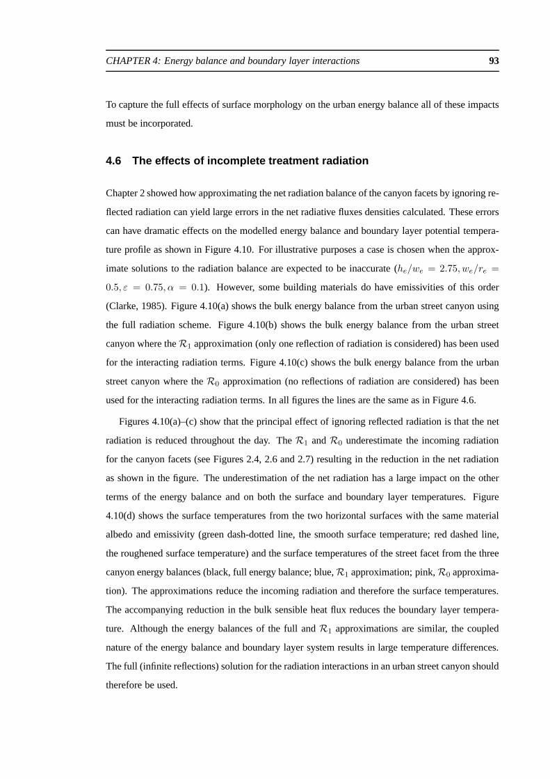
CHAPTER 4: Energy balance and boundary layer interactions 93
To capture the full effects of surface morphology on the urban energy balance all of these impacts
must be incorporated.
4.6 The effects of incomplete treatment radiation
Chapter 2 showed how approximating the net radiation balance of the canyon facets by ignoring re-
flected radiation can yield large errors in the net radiativefluxes densities calculated. These errors
can have dramatic effects on the modelled energy balance andboundary layer potential tempera-
ture profile as shown in Figure 4.10. For illustrative purposes a case is chosen when the approx-
imate solutions to the radiation balance are expected to be inaccurate (he/we = 2.75, we/re =
0.5, ε = 0.75, α = 0.1). However, some building materials do have emissivities ofthis order
(Clarke, 1985). Figure 4.10(a) shows the bulk energy balance from the urban street canyon using
the full radiation scheme. Figure 4.10(b) shows the bulk energy balance from the urban street
canyon where theR1 approximation (only one reflection of radiation is considered) has been used
for the interacting radiation terms. Figure 4.10(c) shows the bulk energy balance from the urban
street canyon where theR0 approximation (no reflections of radiation are considered)has been
used for the interacting radiation terms. In all figures the lines are the same as in Figure 4.6.
Figures 4.10(a)–(c) show that the principal effect of ignoring reflected radiation is that the net
radiation is reduced throughout the day. TheR1 andR0 underestimate the incoming radiation
for the canyon facets (see Figures 2.4, 2.6 and 2.7) resulting in the reduction in the net radiation
as shown in the figure. The underestimation of the net radiation has a large impact on the other
terms of the energy balance and on both the surface and boundary layer temperatures. Figure
4.10(d) shows the surface temperatures from the two horizontal surfaces with the same material
albedo and emissivity (green dash-dotted line, the smooth surface temperature; red dashed line,
the roughened surface temperature) and the surface temperatures of the street facet from the three
canyon energy balances (black, full energy balance; blue,R1 approximation; pink,R0 approxima-
tion). The approximations reduce the incoming radiation and therefore the surface temperatures.
The accompanying reduction in the bulk sensible heat flux reduces the boundary layer tempera-
ture. Although the energy balances of the full andR1 approximations are similar, the coupled
nature of the energy balance and boundary layer system results in large temperature differences.
The full (infinite reflections) solution for the radiation interactions in an urban street canyon should
therefore be used.
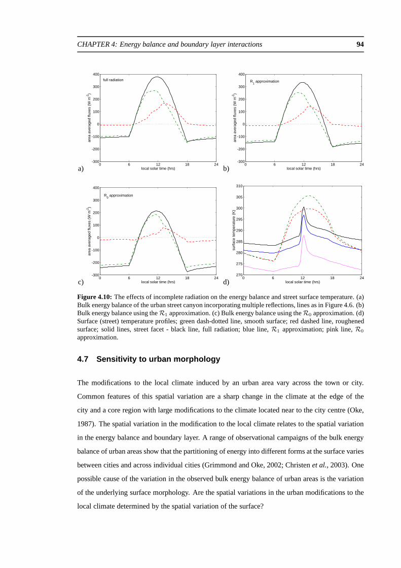
CHAPTER 4: Energy balance and boundary layer interactions 94
a)0 6 12 18 24
-300
-200
-100
0
100
200
300
400
area
ave
rage
d flu
xes
(W m
-2)
local solar time (hrs)
full radiation
b)0 6 12 18 24
-300
-200
-100
0
100
200
300
400
area
ave
rage
d flu
xes
(W m
-2)
local solar time (hrs)
R1 approximation
c)0 6 12 18 24
-300
-200
-100
0
100
200
300
400
area
ave
rage
d flu
xes
(W m
-2)
local solar time (hrs)
R0 approximation
d)0 6 12 18 24
270
275
280
285
290
295
300
305
310
local solar time (hrs)
surf
ace
tem
pera
ture
(K
)
Figure 4.10: The effects of incomplete radiation on the energy balance and street surface temperature. (a)Bulk energy balance of the urban street canyon incorporating multiple reflections, lines as in Figure 4.6. (b)Bulk energy balance using theR1 approximation. (c) Bulk energy balance using theR0 approximation. (d)Surface (street) temperature profiles; green dash-dotted line, smooth surface; red dashed line, roughenedsurface; solid lines, street facet - black line, full radiation; blue line,R1 approximation; pink line,R0
approximation.
4.7 Sensitivity to urban morphology
The modifications to the local climate induced by an urban area vary across the town or city.
Common features of this spatial variation are a sharp changein the climate at the edge of the
city and a core region with large modifications to the climatelocated near to the city centre (Oke,
1987). The spatial variation in the modification to the localclimate relates to the spatial variation
in the energy balance and boundary layer. A range of observational campaigns of the bulk energy
balance of urban areas show that the partitioning of energy into different forms at the surface varies
between cities and across individual cities (Grimmond and Oke, 2002; Christenet al., 2003). One
possible cause of the variation in the observed bulk energy balance of urban areas is the variation
of the underlying surface morphology. Are the spatial variations in the urban modifications to the
local climate determined by the spatial variation of the surface?

CHAPTER 4: Energy balance and boundary layer interactions 95
The urban canyon energy balance model developed in Sections4.1-4.3 is used to investigate
the sensitivity of the coupled energy balance and boundary layer system to surface morphology.
The urban street canyon has two independent morphological parameters, the canyon aspect ratio,
he/we, and the ratiowe/re. In real urban areas both these parameters vary spatially; here the two
parameters are first varied separately and then varied together. In all cases the building height is
constant at 10 m and located at 60N, the day considered is the spring equinox.
4.7.1 Sensitivity to the canyon aspect ratio
A key parameter describing the extent of urbanisation is thecanyon aspect ratio. Highly urbanised
areas tend to have high canyon aspect ratios,he/we > 1, and high building heights. Figure 4.11
shows the diurnal variation of the bulk sensible heat flux (a)and 15 m potential temperature (b)
calculated using the model developed in Sections 4.1-4.3 for a range of canyon aspect ratios. For
these caseswe/re = 0.5, and the canyon was oriented north-south.
Consider first the variation of the bulk sensible heat flux with canyon aspect ratio. Increasing
the canyon aspect ratio decreases the diurnal range and maximum value of the bulk sensible heat
flux. These effects are partly due to the increase in total surface area (Section 4.4). However, the
dominant process occuring is the reduction in the transfer coefficients for the sensible heat flux
densities from the street and wall facets as the canyon aspect ratio increases. A key feature in
Figure 4.11(a) is the delay in the phase of the sensible heat flux, as considered in Section 4.5.1.
This is more pronounced as the canyon aspect ratio is increased resulting in delayed peak values
and delayed transitions to stable conditions in the early evening. Grimmond and Oke (2002) show
a reduction in the magnitude of the sensible heat flux and a delay in its phase with increasing
urbanisation for a range of North American cities.
The variation in the bulk sensible heat flux influences the diurnal variation of the 15 m potential
temperature. The diurnal range is reduced at high canyon aspect ratios, due to both the reduced
surface forcing (Figure 4.11(b)) and the offset in surface temperatures due to the shape factor
effect on the net radiation. The maximum temperature difference between the flat surface and the
urban street canyon occurs at dawn in all cases and shows a rapid change as the canyon ratio is
increased from low values. This increase slows markedly as the canyon aspect ratio increases past
he/we = 1. By night the key terms in the energy balance are the net radiative terms which, as
Chapter 2 showed, vary rapidly aroundhe/we = 0.5. At higher canyon aspect ratios the further
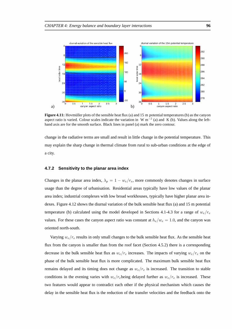
CHAPTER 4: Energy balance and boundary layer interactions 96
a) b)
278
280
282
284
286
288
290
292
0 0.5 1 1.5 2 2.5 3
0
6
12
18
24
30
36
canyon aspect ratio
loca
l sol
ar ti
me
diurnal variation of the 15m potential temperature
Figure 4.11:Hovmuller plots of the sensible heat flux (a) and 15 m potential temperatures (b) as the canyonaspect ratio is varied. Colour scales indicate the variation in W m−2 (a) and K (b). Values along the left-hand axis are for the smooth surface. Black lines in panel (a)mark the zero contour.
change in the radiative terms are small and result in little change in the potential temperature. This
may explain the sharp change in thermal climate from rural tosub-urban conditions at the edge of
a city.
4.7.2 Sensitivity to the planar area index
Changes in the planar area index,λp = 1 − we/re, more commonly denotes changes in surface
usage than the degree of urbanisation. Residential areas typically have low values of the planar
area index; industrial complexes with low broad workhouses, typically have higher planar area in-
dexes. Figure 4.12 shows the diurnal variation of the bulk sensible heat flux (a) and 15 m potential
temperature (b) calculated using the model developed in Sections 4.1-4.3 for a range ofwe/re
values. For these cases the canyon aspect ratio was constantathe/we = 1.0, and the canyon was
oriented north-south.
Varyingwe/re results in only small changes to the bulk sensible heat flux. As the sensible heat
flux from the canyon is smaller than from the roof facet (Section 4.5.2) there is a corresponding
decrease in the bulk sensible heat flux aswe/re increases. The impacts of varyingwe/re on the
phase of the bulk sensible heat flux is more complicated. The maximum bulk sensible heat flux
remains delayed and its timing does not change aswe/re is increased. The transition to stable
conditions in the evening varies withwe/rebeing delayed further aswe/re is increased. These
two features would appear to contradict each other if the physical mechanism which causes the
delay in the sensible heat flux is the reduction of the transfer velocities and the feedback onto the
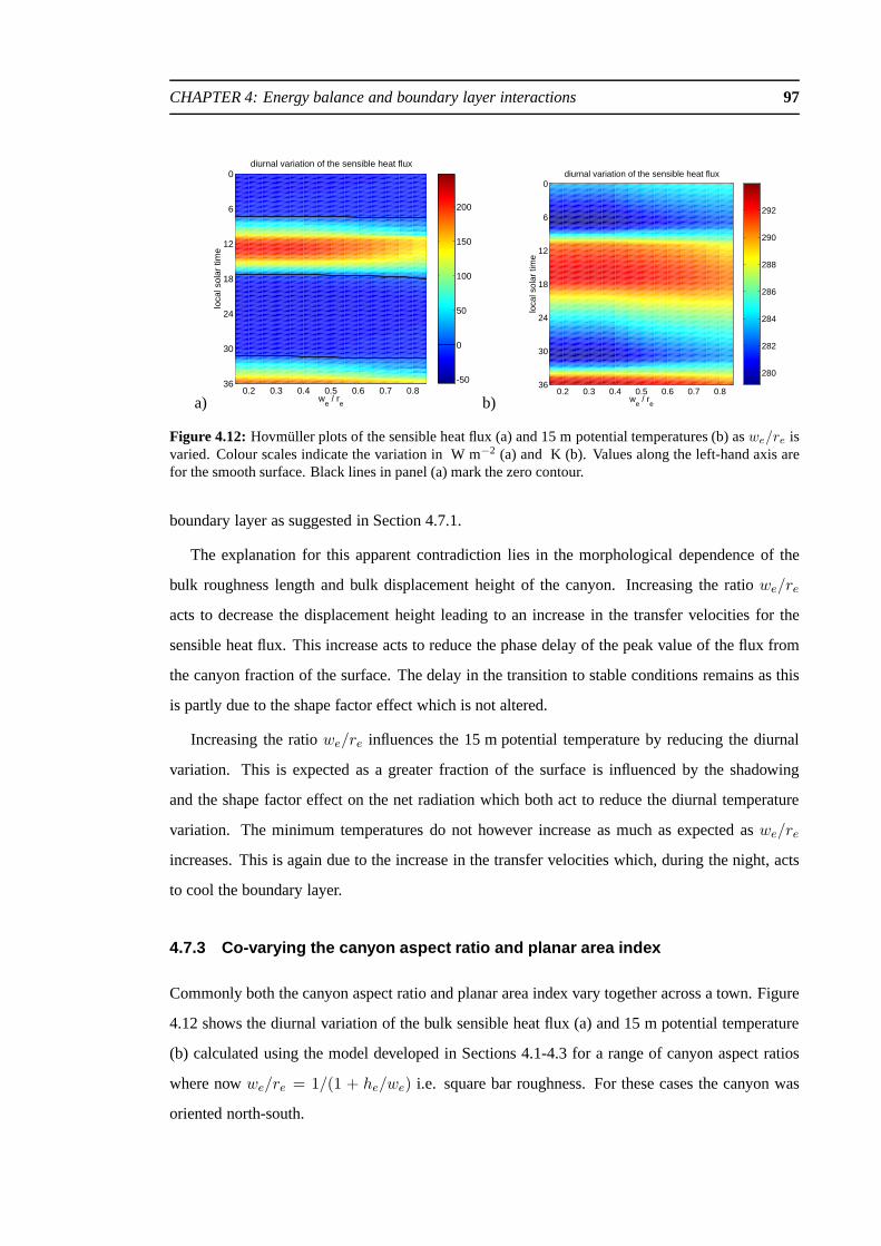
CHAPTER 4: Energy balance and boundary layer interactions 97
a)
-50
0
50
100
150
200
0.2 0.3 0.4 0.5 0.6 0.7 0.8
0
6
12
18
24
30
36
we / r
e
loca
l sol
ar ti
me
diurnal variation of the sensible heat flux
b)
280
282
284
286
288
290
292
0.2 0.3 0.4 0.5 0.6 0.7 0.8
0
6
12
18
24
30
36
we / r
e
loca
l sol
ar ti
me
diurnal variation of the sensible heat flux
Figure 4.12: Hovmuller plots of the sensible heat flux (a) and 15 m potential temperatures (b) aswe/re isvaried. Colour scales indicate the variation in W m−2 (a) and K (b). Values along the left-hand axis arefor the smooth surface. Black lines in panel (a) mark the zerocontour.
boundary layer as suggested in Section 4.7.1.
The explanation for this apparent contradiction lies in themorphological dependence of the
bulk roughness length and bulk displacement height of the canyon. Increasing the ratiowe/re
acts to decrease the displacement height leading to an increase in the transfer velocities for the
sensible heat flux. This increase acts to reduce the phase delay of the peak value of the flux from
the canyon fraction of the surface. The delay in the transition to stable conditions remains as this
is partly due to the shape factor effect which is not altered.
Increasing the ratiowe/re influences the 15 m potential temperature by reducing the diurnal
variation. This is expected as a greater fraction of the surface is influenced by the shadowing
and the shape factor effect on the net radiation which both act to reduce the diurnal temperature
variation. The minimum temperatures do not however increase as much as expected aswe/re
increases. This is again due to the increase in the transfer velocities which, during the night, acts
to cool the boundary layer.
4.7.3 Co-varying the canyon aspect ratio and planar area ind ex
Commonly both the canyon aspect ratio and planar area index vary together across a town. Figure
4.12 shows the diurnal variation of the bulk sensible heat flux (a) and 15 m potential temperature
(b) calculated using the model developed in Sections 4.1-4.3 for a range of canyon aspect ratios
where nowwe/re = 1/(1 + he/we) i.e. square bar roughness. For these cases the canyon was
oriented north-south.

CHAPTER 4: Energy balance and boundary layer interactions 98
a)
-50
0
50
100
150
200
0 0.5 1 1.5 2 2.5 3
0
6
12
18
24
30
36
canyon aspect ratio
loca
l sol
ar ti
me
diurnal variation of the sensible heat flux
b)
278
280
282
284
286
288
290
292
0 0.5 1 1.5 2 2.5 3
0
6
12
18
24
30
36
canyon aspect ratio
loca
l sol
ar ti
me
diurnal variation in 15m potential temperature
Figure 4.13:Hovmuller plots of the sensible heat flux (a) and 15 m potential temperatures (b) as the canyongeometry is varied as square bar roughness. Colour scales indicate the variation in W m−2 (a) and K (b).Values along the left-hand axis are for the smooth surface. Black lines in panel (a) mark the zero contour.
The effects of the initial dip in the transfer velocities forthe sensible heat flux from the street
facet around a canyon aspect ratio ofhe/we = 0.25 (Section 3.6.2) can be clearly seen in both the
bulk sensible heat flux and the 15 m potential temperature particularly during the day. Otherwise
the two effects of varying the canyon aspect ratio and planararea index together cancel to a large
extent. This is a result of the competing effects of the reduction in the transfer velocities as the
canyon aspect ratio and displacement height are increased being balanced by an increase in the
offset of the temperatures due to the shape factor effect.
These plots show that surface geometry is a more important effect than the increase in total
surface area. Ashe/we is increased past 0.5 the diurnal range of the 15 m potential temperature
increases which is counter to the effect expected due to the increase in total surface area (Section
4.4). For instance the difference between the minimum temperatures over the canyon and flat
surfaces for a canyon aspect ratio ofhe/we = 3 is smaller than for a canyon aspect ratio of
he/we = 0.5. This is illustrates that the boundary layer responds to thebulk energy balance. For
the geometry considered, at high canyon aspect ratios the surface resembles a flat but displaced
surface (see Figure 1.5(c)). The bulk energy balance therefore principally resembles that of flat
surface despite the increase in surface area.
4.7.4 Sensitivity to canyon orientation
A geometric factor not considered in detail until now is the orientation of the canyon. Figure 4.14
shows the diurnal variation of the bulk sensible heat flux (a)and 15 m potential temperature (b)

CHAPTER 4: Energy balance and boundary layer interactions 99
a)
-50
0
50
100
150
200
0 45 90 135 180 225 270 315 360
0
6
12
18
24
30
36
canyon orientation
loca
l sol
ar ti
me
diurnal variation of the sensible heat flux
b)
282
284
286
288
290
292
0 45 90 135 180 225 270 315 360
0
6
12
18
24
30
36
canyon orientation
loca
l sol
ar ti
me
diurnal variation of the 15m potential temperature
Figure 4.14:Hovmuller plots of the sensible heat flux (a) and 15 m potential temperatures (b) as the canyonorientation is varied. Colour scales indicate the variation in W m−2 (a) and K (b). Values along the left-hand axis are for the smooth surface. Black lines in panel (a)mark the zero contour.
calculated using the model developed in Sections 4.1-4.3 for the full range of canyon orientations.
For these cases the canyon geometry washe/we = 1.0 andwe/re = 0.5.
Canyon orientation primarily influences the direct component of the solar radiative flux den-
sities (Appendix A). It also influences the transfer velocities for the sensible heat flux through
the relative orientations of the wind and canyon as described in Section 4.2. Given the physical
processes acting it is therefore unsurprising that canyon orientation should play a role. Of the two
processes, the impacts of canyon orientation on the radiation balance are more pronounced. The
boundary layer potential temperature shows a clear asymmetry during the day when the impacts
on the direct solar radiation occur but little asymmetry during the night when only the impacts on
the turbulent fluxes are acting. The variation of the bulk sensible heat flux with canyon orientation
is of a comparable magnitude to the variation with the planararea index or square bar roughness.
Energy balance models for use in numerical weather prediction models should therefore account
for real scale variation in canyon orientation.
4.7.5 Sensitivity to urban morphology: Summary
This work has shown that the impacts of surface morphology onthe bulk energy balance of, and
boundary layer over, an urban area is a key factor determining the modifications to the local climate
by urban areas. The effects of surface morphology on the coupled energy balance/boundary layer
system explains the changes in magnitudes and phases of the terms of the bulk energy balance and
goes towards explaining the observed variation in boundarylayer potential temperature across an

CHAPTER 4: Energy balance and boundary layer interactions 100
urban area (e.g. Oke, 1987). The work reinforces the idea that the canyon aspect ratio is the key
geometric parameter determining the thermal effects of thebuilding array (Okeet al., 1991) but in
a context which includes a turbulent sensible heat flux and aninteracting boundary layer.
The canyon aspect ratio is not the only geometric parameter that is important. Although of
lesser importance, the planar area index does affect the bulk energy balance and the boundary layer
and can counter the effects of increasing the canyon aspect ratio. Similarly, the orientation of the
street canyon affects the coupled system markedly. This orientational effect must be considered
when devising a energy balance model for urban areas for use in operational weather prediction
models where the canyon orientation may not be known and/or poorly defined.
Varying the canyon parameters shows that surface morphology on its own cannot explain a
key observed feature of urban areas, namely the maintenanceof a positive bulk sensible heat flux
through the night (e.g. Okeet al., 1999). In all cases the one-dimensional boundary layer model
gives a stable boundary layer during the night. An explanation is that in this one-dimensional
model the only process which cools the boundary layer is a negative bulk sensible heat flux. During
the night the dominant feature of the energy balance is long-wave radiative cooling at the surface
which, in all cases considered here, cools the surface temperature below that of the overlying
boundary layer air by early evening. To maintain a boundary layer that is cooler than the surface
and thus a positive bulk sensible heat flux during the night asobserved in heat island conditions,
a physical process is needed which cools the boundary layer air ahead of the surface induced
cooling. An investigation into the physical processes which can accomplish this are considered in
Chapter 6.
4.8 Summary and conclusions
Chapter 4 considered the influence of surface morphology on the interactions between the urban
energy balance and overlying boundary layer. An urban energy balance was formulated from
the facet-averaged energy balances of the four facets of an urban street canyon and coupled to a
one-dimensional boundary layer model (Buschet al., 1976).
The influence of surface morphology on the energy balance wasshown to explain several key
features of the energy balance of urban areas. In an urban area the partitioning of energy between
the ground heat flux and the turbulent sensible heat flux is altered to favour the ground heat flux
(e.g. Grimmond and Oke, 2002). The net radiation remains approximately the same with the
CHAPTER 4: Energy balance and boundary layer interactions 101
peak value of the sensible heat flux occuring later and a general reduction in the magnitude of the
sensible heat flux by night (e.g. Cleugh and Oke, 1986). Thesefeatures are explained primarily by
the shape factor effect on the longwave radiation, i.e. someof the incoming long-wave radiation
for the canyon facets originates from the other canyon facets and not the sky (Chapter 2). The
reduction in the transfer velocities for the sensible heat flux due to surface geometry is important
in altering the phase of the terms of the bulk energy balance.
Observed climatological features of the urban boundary layer can also be explained by the
influence of surface morphology on the processes coupling the surface and boundary layer. The
boundary layer over the canyon surface is shown to vary little from that over a flat surface by
day despite the large differences in surface forcing but with significant thermal excesses during
the night (e.g Atkinson, 1985). This results from the depth of the boundary layer over which the
differences in forcing are exerted (deep by day, shallow by night) and illustrates the importance of
the boundary layer in controlling the depth and magnitude ofthe urban heat island (e.g. Arnfield,
2003). Nocturnal urban boundary layers are seen to be deeper, less windy, and less stable than their
rural counterparts (e.g Atkinson, 1985). Here it is shown how surface morphology controls these
differences. The key physical process resulting from surface morphology is the shape factor effect
on the net radiation but other processes such as the increased surface roughness and variation of
the turbulent fluxes with geometry are also important. Theselatter processes are important when
explaining changes in the phase of the individual terms of the bulk energy balance.
The variation of the surface morphological influences on theenergy balance and boundary
system also explain, to some degree, the spatial patterns ofthe urban modifications to the local
climate. For instance the shape factor effect has a rapid onset as the canyon aspect ratio is increased
past 0.1, which may explain the sharp transition in climate at the edge of cities (e.g. Oke, 1987).
Additionally, the core regions of cities experience the largest perturbations associated with the
largest canyon aspect ratios and therefore largest shape factor effects. Although the canyon aspect
ratio is the dominant geometrical ratio, the planar area index does influence the energy balance
and boundary layer most notably through the induced changesto the turbulent exchange. Surface
morphology is, however, unable, on its own, to explain the maintenance of positive sensible heat
fluxes and neutral urban boundary layers during the night. This key observation of the urban
boundary layer is considered further in Chapter 6.
CHAPTER FIVE
A simplified urban energy balance
5.1 Intoduction
The modifications to the local climate induced by urban areascan be instantaneously large and
qualitatively important for their occupants (Oke, 1987; Dabbertet al., 2000) therefore requiring
accurate forecasts. Evidence for the urban modification of the local weather comes from rainfall
distribution changes (e.g. Cotton and Pielke, 1995), the delay of frontal systems (e.g. Loose and
Bornstein, 1977; Bornstein and Thompson, 1981) and the trigggering of convection (e.g. Bornstein
and Lin, 2000; Rozoff and Adegoke, 2003) as well as the urban heat island studies (see Arnfield,
2003, for a review). Urban areas, however, remain a small fraction of the total land surface area of
the Earth and there is little evidence to indicate that urbanareas significantly modify the weather
away from the local area. A possible method of forecasting the weather within urban areas is to
take forecasts from numerical weather prediction models that do not incorporate urban areas and
statistically downscale offline for the urban areas. Given the degree of interaction between the
boundary layer and urban energy balance shown in the previous chapters it is unlikely that this
approach would be satisfactory across the full range of urban surfaces and synoptic conditions.
This poses a problem of how best to, and the required detail needed to, incorporate urban areas
into numerical weather prediction models.
At the heart of this problem is the issue of scale (Section 1.1). The previous chapters showed,
and much of the current understanding indicates (Britter and Hanna, 2003), that much of the impact
of urban areas is determined by physical processes acting atthe street scale and the subsequent
feedback through the boundary layer. Numerical weather prediction models act at the city (or at
most the neighbourhood) scale seeking to predict the bulk effects and not the fine scale features.
Methods must therefore be identified which enable the impacts of the street scale processes on the
102

CHAPTER 5: A simplified urban energy balance 103
neighbourhood scale to be captured which rely only on information known at the neighbourhood
scale and without the complexity of working at the street scale.
Accompanying this issue of scale is an issue of complexity. The urban canyon models possess
a large number parameters specific to the street scale which must be specified (e.g. Masson, 2000).
Two issues relate to these parameters when working within numerical weather prediction models.
Firstly, working at the neighbourhood scale implies that the variation in these properties across
the neighbourhood cannot be captured. Which value of these parameters is representative of the
neighbourhood and how should they be determined? Grossman-Clarke et al. (2003) illustrates
the complexity required to calculate some of these parameters from reality at only a moderate
resolution. Secondly, the averaging length scale on which these parameters are calculated requires
careful consideration. Is it possible to relate this lengthscale to the resolution of the model or
some physically relevant length scale? Within climate modelling, where whole cities can fit into
one grid box, both of these issues will be even more complex.
The parameterization of the surface energy balance within numerical weather prediction mod-
els must be kept as simple as possible. All of the major types of urban energy balance model
(Section 1.3) have been incorporated into mesoscale weather prediction models (Best, 1998a;
Taha, 1999; Massonet al., 2002; Martilli et al., 2002). Only the simple energy balance model
of Best (1998a, 1999) is currently operational; the other models have been used to investigate
specific events such as the heat island and urban circulations (Taha, 1999; Lemonsu and Masson,
2002; Martilli, 2002). The current Met Office Unified Model surface exchange scheme, MOSES
(Esseryet al., 2001, 2003), is configured for surface heterogeneity but isnot configured to allow
for directly interacting surfaces. The urban street canyonmodel presented in Chapter 4 has direct
interactions between the wall and street facets in both the radiative and turbulent terms (Sections
4.2.1 and 4.2.2). It would be desirable therefore if these interaction terms can be approximated.
This chapter therefore focusses on possible ways to approximate the urban canyon energy bal-
ance so that it can be incorporated into numerical weather prediction models yet which preserve
the most significant features of the urban energy balance as highlighted in Chapter 4. Two ap-
proximations to the full urban street canyon energy balancemodel are presented in Section 5.2.
A comparison between the two approximations and the full scheme is presented in Section 5.3.
Finally, results from this chapter will be used to address the complexity of the model of the urban
energy balance model required and the specification of required input parameters in numerical
weather prediction models.
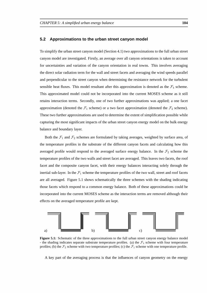
CHAPTER 5: A simplified urban energy balance 104
5.2 Approximations to the urban street canyon model
To simplify the urban street canyon model (Section 4.1) two approximations to the full urban street
canyon model are investigated. Firstly, an average over allcanyon orientations is taken to account
for uncertainties and variation of the canyon orientation in real towns. This involves averaging
the direct solar radiation term for the wall and street facets and averaging the wind speeds parallel
and perpendicular to the street canyon when determining theresistance network for the turbulent
sensible heat fluxes. This model resultant after this approximation is denoted as theF4 scheme.
This approximated model could not be incorporated into the current MOSES scheme as it still
retains interaction terms. Secondly, one of two further approximations was applied; a one facet
approximation (denoted theF1 scheme) or a two facet approximation (denoted theF2 scheme).
These two further approximations are used to determine the extent of simplification possible while
capturing the most significant impacts of the urban street canyon energy model on the bulk energy
balance and boundary layer.
Both theF1 andF2 schemes are formulated by taking averages, weighted by surface area, of
the temperature profiles in the substrate of the different canyon facets and calculating how this
averaged profile would respond to the averaged surface energy balance. In theF2 scheme the
temperature profiles of the two walls and street facet are averaged. This leaves two facets, the roof
facet and the composite canyon facet, with their energy balances interacting solely through the
inertial sub-layer. In theF1 scheme the temperature profiles of the two wall, street and roof facets
are all averaged. Figure 5.1 shows schematically the three schemes with the shading indicating
those facets which respond to a common energy balance. Both of these approximations could be
incorporated into the current MOSES scheme as the interaction terms are removed although their
effects on the averaged temperature profile are kept.
a) b) c)
Figure 5.1: Schematic of the three approximations to the full urban street canyon energy balance model- the shading indicates separate substrate temperature profiles. (a) theF4 scheme with four temperatureprofiles; (b) theF2 scheme with two temperature profiles; (c) theF1 scheme with one temperature profile.
A key part of the averaging process is that the influences of canyon geometry on the energy

CHAPTER 5: A simplified urban energy balance 105
balances are maintained. Consider first theF2 scheme; a temperature profileTF2is formulated as
the average, weighted by surface area, of the temperature profilesTst, Tuw andTdw together with
an average volumetric heat capacity for the three facetscs F2, namely
(we + 2he)TF2= weTst + he (Tuw + Tdw) , (5.1)
(we + 2he) csF2= wecs st + he (cs uw + cs dw) . (5.2)
The energy balance to which this temperature profile responds is given as
∆z cs F2
∂TF2 1/2
∂t=
∆z
we + 2he
[
wecs st
∂Tst 1/2
∂t+ hecs uw
∂Tuw 1/2
∂t+ hecs dw
∂Tdw 1/2
∂t
]
, (5.3)
=∆z
we + 2he
[
we(1 − αst)Ksfst + he(1 − αuw)Ksfuw + he(1 − αdw)Ksfdw + . . . ,
where the subscript1/2 refers to the surface layer of the substrate and the tilde indicates the orien-
tational average. The approximationTst = Tuw = Tdw = TF2is used in all terms including the
interaction terms present on expanding the square brackets.
Applying the approximationTst = Tuw = Tdw = TF2can introduce differences in the bulk
energy balance obtained from theF4 andF2 schemes as well as the energy balances for the indi-
vidual facets. These differences arise from the averaging of terms involving the co-variation of the
temperature profile and facet specific parameters. For example the sensible heat flux density out
of the canyon air volume is given byHc = ρcpwc (θ(z2) − Tc), whereTc is a linear combination
of the facets’ surface temperatures as given by Equation (4.16). Unless the transfer velocitieswst,
wuw andwdw are equal then applying the approximation will introduce anerror inTc and there-
foreHc from theF4 andF2 schemes will differ. Similarly differences between the twoschemes
can arise through the co-variation of the temperatures of the different facets with the direct solar
radiative flux densities, with the thermal conductivities or heat capacities of the substrates, or with
the shape factor effect on the longwave radiative flux densities. Part of this work is to assess the
importance of these co-varying terms in determining the bulk energy balance of an urban street
canyon. Differences between the two schemes can be reinforced via a feedback occuring through
the influence of stability on the turbulent mixing in the boundary layer and the subsequent impacts
on the bulk sensible heat flux.

CHAPTER 5: A simplified urban energy balance 106
The differences between theF4 andF2 schemes imposed by averaging these co-variating terms
are however expected to be small for two reasons. Firstly, the differences between the tempera-
ture profiles of the separate facets (theF4 scheme) and the averaged temperature profile (theF2
scheme) are much smaller than absolute value of the temperature. This implies that the differences
in the emitted longwave flux densities will be small. Secondly, the effects of surface morphology
on the facet specific parameters and the individual terms of the energy balance are commonly a
factor of two or more. This is commonly much greater than the variation of the facet specific
parameters between the different facets. It follows that the differences between the two schemes
resulting from averaging the three temperature profiles will be small when compared to those as-
sociated with the combined effects of surface morphology. The exception to this general rule are
the impacts of averaging the direct solar radiative flux densities which is the primary cause of
the differences between the facets (Section 4.5). It follows that convoluted canyon morphologies,
which impose greatly different direct solar flux densities on the wall and street canyon facets, are
likely to impose large differences between theF4 andF2 schemes.
In practical terms, the influence of surface morphology on the resistances to transport (r1–r8)
and on the canyon air temperature (Equation (4.16)) is kept but the possible differences between
the surface temperatures in Equation (4.16) have been removed. Similarly, the surface tempera-
tures used in the calculation of the emitted longwave radiation from the canyon facets are now
equal but the effects of surface morphology on the shape factor effect and multiple reflections of
radiation (Chapter 2) are kept. In this way the influence of surface morphology on the radiative
and turbulent sensible heat fluxes is preserved but now thereis only one surface and substrate
temperature for the three canyon facets.
TheF1 scheme is formulated in an equivalent way. A temperature profile TF1is formulated as
the average, weighted by surface area, of the temperature profiles of all four facets together with
an averaged volumetric heat capacity for the facetscs F1, namely
(re + 2he)TF1= weTst + (re −we)Trf + he (Tuw + Tdw) , (5.4)
(re + 2he) csF1= wecs st + (re − we)cs rf + he (cs uw + cs dw) . (5.5)

CHAPTER 5: A simplified urban energy balance 107
The energy balance to which this averaged temperature profile responds is
∆z cs F1
∂TF1 1/2
∂t=
∆z
re + 2he
[
wecs st
∂Tst 1/2
∂t
+(re − we)cs rf
∂Trf 1/2
∂t+ hecs uw
∂Tuw 1/2
∂t+ hecs dw
∂Tdw 1/2
∂t
]
. (5.6)
Differences between theF4 andF1 schemes occur as with theF2 scheme. Here, however the
differences between the co-variation terms of the roof facet and of the street and wall facets are
larger than those between the street and wall facets and so averaging over the co-varying terms is
expected to lead to larger differences.
The evolution of the temperature profiles (Equations (5.1) and (5.4)) requires two boundary
conditions. The first boundary condition is given by expanding Equations (5.3) or (5.6) but the
second boundary condition is a final consideration. This second boundary condition is only of
concern if the depth of the substrate is shallow enough that the diurnal signal is influenced by
the boundary condition (Section 4.5). Here this boundary condition is a weighted average of the
boundary conditions on the facet substrate temperature profiles and the depth of these substrates
is sufficient that the boundary condition does not play a significant role.
5.3 Comparison between the F1, F2 and F4 schemes
For any simplification of the urban street canyon energy balance to be useful, the bulk energy
balance and boundary layer potential temperature profiles should be similar to theF4 scheme.
The three schemes were used for the same forcing conditions as Section 4.5 for a range of canyon
geometries.
Figures 5.2 and 5.3 show the differences in each of the terms of the energy balance between the
F2 andF4 schemes (left panels) andF1 andF4 schemes (right panels). In each case the solid line
is the difference in net radiation, the dashed line the difference in the bulk sensible heat flux and
the dash-dotted line the difference in the ground heat flux. The left and right panels are plotted on
the same vertical axis for ease of comparison.
Figure 5.2 shows how the different schemes fare as the canyonaspect ratio is varied for a con-
stant value ofwe/re = 0.5. As the averaging of the direct solar radiative flux densities imposes
the largest differences between the schemes it is expected that at low canyon aspect ratios the

CHAPTER 5: A simplified urban energy balance 108
F2 − F4 F1 −F4
a)0 3 6 9 12 15 18 21 24
-10
-8
-6
-4
-2
0
2
4
6
8
10
local solar time (hrs)
diffe
renc
e be
twee
n bu
lk e
nerg
y ba
lanc
es (
W m
-2)
b)0 3 6 9 12 15 18 21 24
-10
-8
-6
-4
-2
0
2
4
6
8
10
local solar time (hrs)
diffe
renc
e be
twee
n bu
lk e
nerg
y ba
lanc
es (
W m
-2)
c)0 3 6 9 12 15 18 21 24
-25
-20
-15
-10
-5
0
5
10
15
20
25
local solar time (hrs)
diffe
renc
e be
twee
n bu
lk e
nerg
y ba
lanc
es (
W m
-2)
d)0 3 6 9 12 15 18 21 24
-25
-20
-15
-10
-5
0
5
10
15
20
25
local solar time (hrs)
diffe
renc
e be
twee
n bu
lk e
nerg
y ba
lanc
es (
W m
-2)
e)0 3 6 9 12 15 18 21 24
-50
-40
-30
-20
-10
0
10
20
30
40
50
local solar time (hrs)
diffe
renc
e be
twee
n bu
lk e
nerg
y ba
lanc
es (
W m
-2)
f)0 3 6 9 12 15 18 21 24
-50
-40
-30
-20
-10
0
10
20
30
40
50
local solar time (hrs)
diffe
renc
e be
twee
n bu
lk e
nerg
y ba
lanc
es (
W m
-2)
Figure 5.2: Differences between the energy balances of the three approximations. Left panels, differencesbetween theF2 andF4; right panels, differences between theF1 andF4. Black solid lines, difference in thenet radiative flux; green dash-dotted lines, difference in the ground heat flux; red dashed lines, difference inthe sensible heat flux. Panels (a) and (b)he/we = 0.25; panels (c) and (d)he/we = 1.0; panels (e) and (f)he/we = 2.0; all panelswe/re = 0.5.
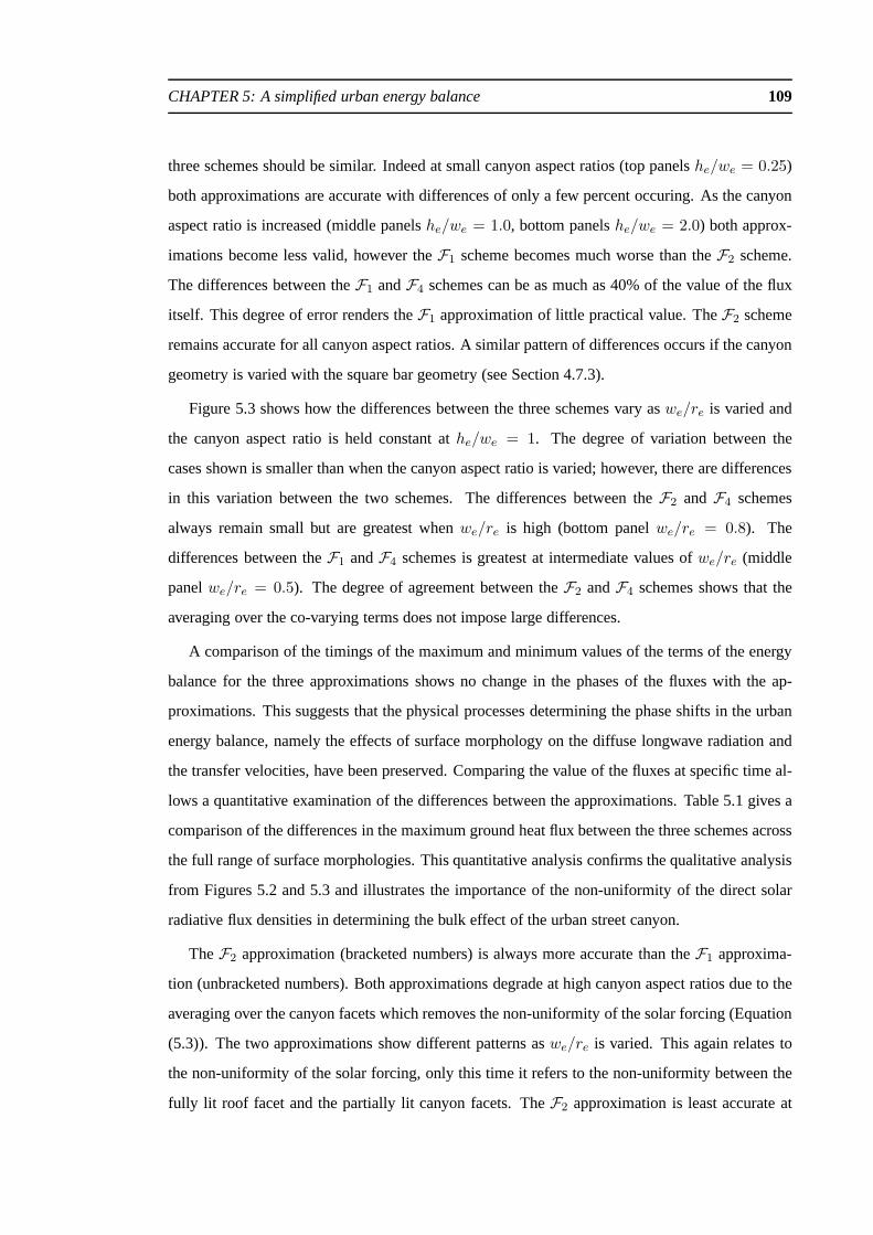
CHAPTER 5: A simplified urban energy balance 109
three schemes should be similar. Indeed at small canyon aspect ratios (top panelshe/we = 0.25)
both approximations are accurate with differences of only afew percent occuring. As the canyon
aspect ratio is increased (middle panelshe/we = 1.0, bottom panelshe/we = 2.0) both approx-
imations become less valid, however theF1 scheme becomes much worse than theF2 scheme.
The differences between theF1 andF4 schemes can be as much as 40% of the value of the flux
itself. This degree of error renders theF1 approximation of little practical value. TheF2 scheme
remains accurate for all canyon aspect ratios. A similar pattern of differences occurs if the canyon
geometry is varied with the square bar geometry (see Section4.7.3).
Figure 5.3 shows how the differences between the three schemes vary aswe/re is varied and
the canyon aspect ratio is held constant athe/we = 1. The degree of variation between the
cases shown is smaller than when the canyon aspect ratio is varied; however, there are differences
in this variation between the two schemes. The differences between theF2 andF4 schemes
always remain small but are greatest whenwe/re is high (bottom panelwe/re = 0.8). The
differences between theF1 andF4 schemes is greatest at intermediate values ofwe/re (middle
panelwe/re = 0.5). The degree of agreement between theF2 andF4 schemes shows that the
averaging over the co-varying terms does not impose large differences.
A comparison of the timings of the maximum and minimum valuesof the terms of the energy
balance for the three approximations shows no change in the phases of the fluxes with the ap-
proximations. This suggests that the physical processes determining the phase shifts in the urban
energy balance, namely the effects of surface morphology onthe diffuse longwave radiation and
the transfer velocities, have been preserved. Comparing the value of the fluxes at specific time al-
lows a quantitative examination of the differences betweenthe approximations. Table 5.1 gives a
comparison of the differences in the maximum ground heat fluxbetween the three schemes across
the full range of surface morphologies. This quantitative analysis confirms the qualitative analysis
from Figures 5.2 and 5.3 and illustrates the importance of the non-uniformity of the direct solar
radiative flux densities in determining the bulk effect of the urban street canyon.
TheF2 approximation (bracketed numbers) is always more accuratethan theF1 approxima-
tion (unbracketed numbers). Both approximations degrade at high canyon aspect ratios due to the
averaging over the canyon facets which removes the non-uniformity of the solar forcing (Equation
(5.3)). The two approximations show different patterns aswe/re is varied. This again relates to
the non-uniformity of the solar forcing, only this time it refers to the non-uniformity between the
fully lit roof facet and the partially lit canyon facets. TheF2 approximation is least accurate at

CHAPTER 5: A simplified urban energy balance 110
F2 − F4 F1 −F4
a)0 3 6 9 12 15 18 21 24
-25
-20
-15
-10
-5
0
5
10
15
20
25
local solar time (hrs)
diffe
renc
e be
twee
n bu
lk e
nerg
y ba
lanc
es (
W m
-2)
b)0 3 6 9 12 15 18 21 24
-25
-20
-15
-10
-5
0
5
10
15
20
25
local solar time (hrs)
diffe
renc
e be
twee
n bu
lk e
nerg
y ba
lanc
es (
W m
-2)
c)0 3 6 9 12 15 18 21 24
-25
-20
-15
-10
-5
0
5
10
15
20
25
local solar time (hrs)
diffe
renc
e be
twee
n bu
lk e
nerg
y ba
lanc
es (
W m
-2)
d)0 3 6 9 12 15 18 21 24
-25
-20
-15
-10
-5
0
5
10
15
20
25
local solar time (hrs)
diffe
renc
e be
twee
n bu
lk e
nerg
y ba
lanc
es (
W m
-2)
e)0 3 6 9 12 15 18 21 24
-25
-20
-15
-10
-5
0
5
10
15
20
25
local solar time (hrs)
diffe
renc
e be
twee
n bu
lk e
nerg
y ba
lanc
es (
W m
-2)
f)0 3 6 9 12 15 18 21 24
-25
-20
-15
-10
-5
0
5
10
15
20
25
local solar time (hrs)
diffe
renc
e be
twee
n bu
lk e
nerg
y ba
lanc
es (
W m
-2)
Figure 5.3: Differences between the energy balances of the three approximations. Left panels, differencesbetween theF2 andF4; right panels, differences between theF1 andF4. Black solid lines, difference in thenet radiative flux; green dash-dotted lines, difference in the ground heat flux; red dashed lines, difference inthe sensible heat flux. Panels (a) and (b)we/re = 0.2; panels (c) and (d)we/re = 0.5; panels (e) and (f)we/re = 0.8; all panelshe/we = 1.0.

CHAPTER 5: A simplified urban energy balance 111
Table 5.1: Difference (%) in the maximum bulk ground heat flux from the four facet model and the twoapproximate models for a range of canyon geometries. Unbracketed numbers refer to theF1 approximation;bracketed numbers refer to theF2 approximation.
we/re
he/we
0.25 0.5 1.0 2.0 4.0
0.2 1.0 (<0.1) 3.5 (0.4) 8.2 (0.3) 17.6 (0.2) 26.7 (0.1)0.35 1.1 (0.1) 3.2 (0.2) 8.0 (0.4) 18.6 (0.4) 26.5 (0.6)0.5 1.2 (0.1) 2.9 (0.3) 7.9 (0.5) 16.9 (0.5) 20.5 (1.2)0.65 1.1 (0.2) 2.7 (0.5) 7.3 (0.7) 10.2 (0.7) 14.6 (0.9)0.8 0.9 (0.2) 1.0 (0.3) 4.8 (0.6) 6.3 (0.6) 7.5 (0.7)
high values ofwe/re. The averaging of the solar forcing over the canyon facets ismost prominent
for these surface morphologies as the non-uniformity between the roof and canyon is preserved.
Conversely, theF1 approximation, with the additional averaging over the rooffacet, is least valid
at low to mid values ofwe/re. This reflects both averaging across fully lit and partiallylit surfaces
and the surface area onto which the direct solar radiative flux is impinging (Equation (5.6)). The
values of these differences shows that for a wide range of canyon morphologies theF2 approx-
imation is sufficiently accurate that other uncertainties in the model will introduce larger errors
than this approximation. However, there is only a limited range of canyon morphologies where
theF1 approximation is sufficiently accurate for use.
Figure 4.10 showed that small differences in the bulk energybalance can result in large differ-
ences in the boundary layer temperature profile. Figure 5.4 shows the impacts that the differences
in the bulk energy balances from the three schemes have on theboundary layer potential tem-
perature for the case study considered in Section 4.5. The black solid line is the boundary layer
potential temperature from theF4 scheme, the red dashed line is that from theF2 scheme, and
the green dash-dotted line that from theF1 scheme at midday (left panel) and midnight (right
panel). The differences between the potential temperatureprofiles show the same characteristics
as in Section 4.5.3 with small differences during the day andlarger differences at night relating as
before to the depth of the boundary layer on which the different surface forcings act. Reflecting
the small differences between the bulk energy balances fromtheF2 andF4 schemes, there is no
distinguishable differences between the potential temperature profiles from these two schemes. A
larger difference is observed in the potential temperatureprofiles from theF1 andF4 schemes at
midnight, which is sufficient to invalidate the approximation.
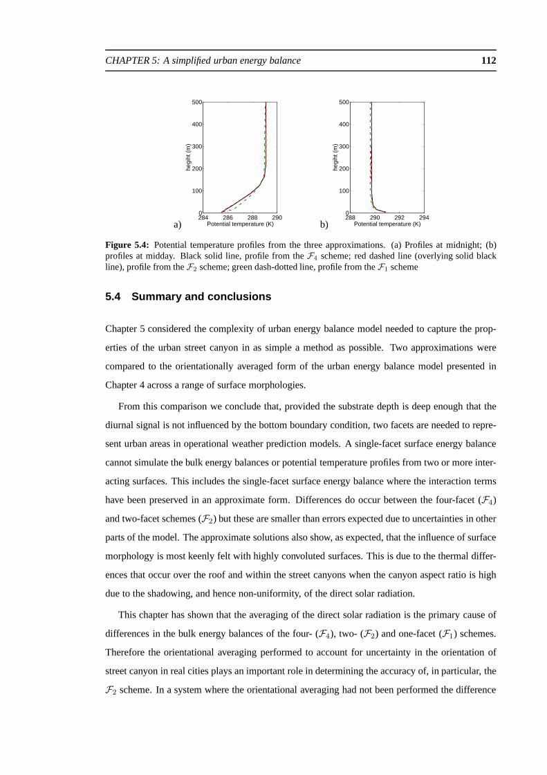
CHAPTER 5: A simplified urban energy balance 112
a)284 286 288 2900
100
200
300
400
500
Potential temperature (K)
hegi
ht (
m)
b)288 290 292 2940
100
200
300
400
500
Potential temperature (K)
hegi
ht (
m)
Figure 5.4: Potential temperature profiles from the three approximations. (a) Profiles at midnight; (b)profiles at midday. Black solid line, profile from theF4 scheme; red dashed line (overlying solid blackline), profile from theF2 scheme; green dash-dotted line, profile from theF1 scheme
5.4 Summary and conclusions
Chapter 5 considered the complexity of urban energy balancemodel needed to capture the prop-
erties of the urban street canyon in as simple a method as possible. Two approximations were
compared to the orientationally averaged form of the urban energy balance model presented in
Chapter 4 across a range of surface morphologies.
From this comparison we conclude that, provided the substrate depth is deep enough that the
diurnal signal is not influenced by the bottom boundary condition, two facets are needed to repre-
sent urban areas in operational weather prediction models.A single-facet surface energy balance
cannot simulate the bulk energy balances or potential temperature profiles from two or more inter-
acting surfaces. This includes the single-facet surface energy balance where the interaction terms
have been preserved in an approximate form. Differences do occur between the four-facet (F4)
and two-facet schemes (F2) but these are smaller than errors expected due to uncertainties in other
parts of the model. The approximate solutions also show, as expected, that the influence of surface
morphology is most keenly felt with highly convoluted surfaces. This is due to the thermal differ-
ences that occur over the roof and within the street canyons when the canyon aspect ratio is high
due to the shadowing, and hence non-uniformity, of the direct solar radiation.
This chapter has shown that the averaging of the direct solarradiation is the primary cause of
differences in the bulk energy balances of the four- (F4), two- (F2) and one-facet (F1) schemes.
Therefore the orientational averaging performed to account for uncertainty in the orientation of
street canyon in real cities plays an important role in determining the accuracy of, in particular, the
F2 scheme. In a system where the orientational averaging had not been performed the difference
CHAPTER 5: A simplified urban energy balance 113
between the solar fluxes for the wall and street facets is greater and therefore theF2 scheme
would not perform as well. However, the sensitivity to canyon orientation of the full canyon
energy balance model is sufficiently large (Section 4.7.4) that unless there is a known preferred
canyon orientation the orientationally averaged street canyon energy balance should be used.
These approximations do not address the complexity of the input parameters needed. The
surface material properties are now averaged and so cannot reasonably take measured values and as
such now resemble tunable parameters. Other parameters such as the mean building height, canyon
aspect ratio, planar area index and bulk roughness length remain tied to the surface morphology
and require determining from the surface land usage. In addressing the length scale over which
these properties should be averaged there are two natural criteria. Firstly, parameter changes on
less than two grid lengths act as numerical noise. Secondly,Coceal and Belcher (2004) and Barlow
et al. (2004) show there is an adjustment length scale for the mean wind and turbulent exchange
when a flow impacts on an array of buildings. Averaging over a length scale less than either of
these two lengths is therefore unreasonable. Chapter 6 willaddress this issue further.
Finally, Chapters 4 and 5 have shown that all aspects of surface morphology play an important
role in determining the urban impact on the local climate. Inparticular, any model for the urban
energy balance which does not include the impacts of surfacemorphology on the radiation balance,
on the bulk roughness length and displacement height and on the turbulent exchange is unlikely to
be valid across the full range of urban surfaces.
CHAPTER SIX
Adjustment of the boundary layer over urban areas
6.1 Introduction
Much consideration has gone into understanding the impactsof urban areas on the local climate
in terms of the characteristics of the local buildings (e.g.morphology, material properties (Oke
et al., 1991)). In particular, the influences that these characteristics have on the energy balance
and boundary layer system must explain many of the observed differences between urban areas
and their rural surroundings. Clear relationships do existbetween some climate diagnostics and
these characteristic properties of urban areas (e.g Oke, 1987). However, the hoped-for correlation
between the spatial variation in the surface morphology andthe spatial variation of the urban
impacts is not found. For instance, Barringet al. (1985) show that while the spatial variation of
the building geometry and the differences in the street surface temperature in Malmo, Sweden is
highly correlated, the correlation with the differences innear-surface air temperature (the urban
heat island) is much smaller and often not statistically significant. Now the interactions between
the surface energy balance and the boundary layer are key in determining the urban impacts on
the climate. Therefore to fully understand the causes of these impacts both the surface and the
boundary layer need to be correct.
Chapter 4 considered the effects of surface morphology on the energy balance and boundary
layer in a fully equilibrated, one-dimensional, scenario.The spatial scale of most urban areas (1–
10 km) is usually much less than the fetch required to establish a fully equilibrated boundary layer
(e.g. Garratt, 1992). Additionally, urban areas themselves are rarely homogeneous because the
building characteristics typically vary on short (100’s m)length scales. The continual adjustment
of the boundary layer as it progresses across an urban area istherefore likely to play a key role in
determining the impact of an urban area.
114

CHAPTER 6: Adjustment of the boundary layer over urban areas 115
The equilibrated scenarios considered in Chapter 4 showed that many observed features of ur-
ban areas can be explained by the effects of surface morphology on the energy balance. However,
some key observed features of the urban impact were not satisfactorily captured. Firstly, the diur-
nal variation in the atmospheric urban heat island is commonly observed to peak a few hours after
dusk (Oke, 1987), whereas the one-dimensional model has this peaking at dawn. Secondly, the
potential temperature profiles of the boundary layers over urban areas and their rural surroundings
approach each other at high altitudes (Oke and East, 1971) unlike the one-dimensional simula-
tions. Finally, the bulk sensible heat flux is observed to remain positive over night (e.g. Okeet al.,
1999) whereas the one-dimensional model cannot sustain a positive heat flux after sunset. This is
particularly important for applications considering pollution dispersal as the degree of turbulent
dispersion is determined by the stability of the boundary layer.
a)0 3 6 9 12 15 18 21 24
275
280
285
290
295
300
305
local solar time (hrs)
Eas
t fac
ing
wal
l sur
face
tem
pera
ture
(K
)
b)0 3 6 9 12 15 18 21 24
-50
0
50
100
150
200
local solar time (hrs)
bulk
sen
sibl
e he
at fl
ux (
W m
-2)
Figure 6.1: Diurnal profiles of the surface temperature of the east facing wall (a) and the bulk sensible heatflux (b) calculated using the coupled canyon energy balance and boundary layer model of Chapter 4. Solidline, case where the wall and roof facet internal temperatures vary with a zero flux boundary condition;dash-dotted line, case where the internal building temperature is raised but still varies according to a zeroflux boundary condition; dotted line, the internal buildingtemperature is raised and fixed (the case shownin Chapter 4); dashed line, as dotted line with the material properties of the wall facets altered so that
the depth of penetration of the diurnal temperature signal(
D =(
86400k/
πcs)1/2
)
is doubled. This is
representative of an uninsulated wall.
A range of physical mechanisms have been proposed to explainthe maintenance of neutral
nocturnal boundary layers including changes in the building material properties, increased storage
of energy during the day which is then released at night and anthropogenic heat sources (e.g.
Oke, 1987). Sensitivity studies with the coupled energy balance-boundary layer model show that
the stable nocturnal boundary layers are always generated in a one-dimensional setting. Varying
model properties such as the surface material conductance or heat capacity and raising and fixing
the internal building temperature do play a significant rolein determining the substrate temperature
profiles (see Figure 6.1(a)). However, none of these changesresults in positive nocturnal bulk
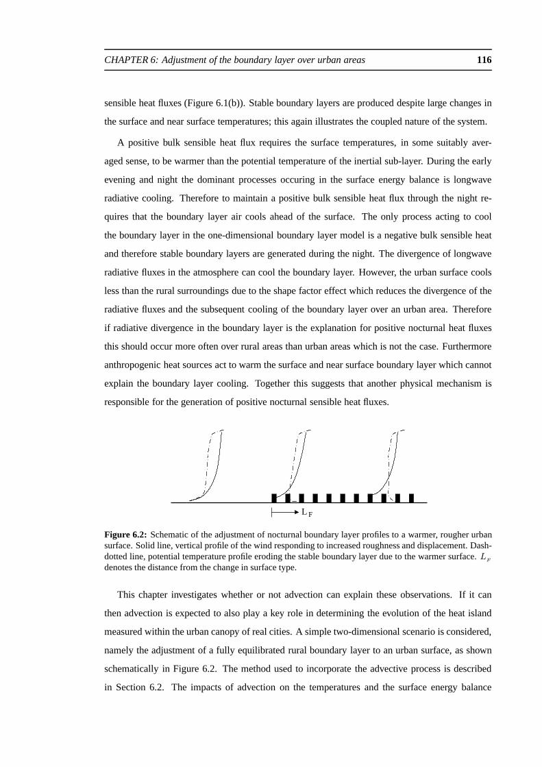
CHAPTER 6: Adjustment of the boundary layer over urban areas 116
sensible heat fluxes (Figure 6.1(b)). Stable boundary layers are produced despite large changes in
the surface and near surface temperatures; this again illustrates the coupled nature of the system.
A positive bulk sensible heat flux requires the surface temperatures, in some suitably aver-
aged sense, to be warmer than the potential temperature of the inertial sub-layer. During the early
evening and night the dominant processes occuring in the surface energy balance is longwave
radiative cooling. Therefore to maintain a positive bulk sensible heat flux through the night re-
quires that the boundary layer air cools ahead of the surface. The only process acting to cool
the boundary layer in the one-dimensional boundary layer model is a negative bulk sensible heat
and therefore stable boundary layers are generated during the night. The divergence of longwave
radiative fluxes in the atmosphere can cool the boundary layer. However, the urban surface cools
less than the rural surroundings due to the shape factor effect which reduces the divergence of the
radiative fluxes and the subsequent cooling of the boundary layer over an urban area. Therefore
if radiative divergence in the boundary layer is the explanation for positive nocturnal heat fluxes
this should occur more often over rural areas than urban areas which is not the case. Furthermore
anthropogenic heat sources act to warm the surface and near surface boundary layer which cannot
explain the boundary layer cooling. Together this suggeststhat another physical mechanism is
responsible for the generation of positive nocturnal sensible heat fluxes.
L F
Figure 6.2: Schematic of the adjustment of nocturnal boundary layer profiles to a warmer, rougher urbansurface. Solid line, vertical profile of the wind respondingto increased roughness and displacement. Dash-dotted line, potential temperature profile eroding the stable boundary layer due to the warmer surface.L
F
denotes the distance from the change in surface type.
This chapter investigates whether or not advection can explain these observations. If it can
then advection is expected to also play a key role in determining the evolution of the heat island
measured within the urban canopy of real cities. A simple two-dimensional scenario is considered,
namely the adjustment of a fully equilibrated rural boundary layer to an urban surface, as shown
schematically in Figure 6.2. The method used to incorporatethe advective process is described
in Section 6.2. The impacts of advection on the temperaturesand the surface energy balance

CHAPTER 6: Adjustment of the boundary layer over urban areas 117
are described in Section 6.3 and finally, the implications ofthis work for operational numerical
weather prediction models are considered in Section 6.4.
6.2 Representation of advection in a one-dimensional setti ng
The adjustment of the boundary layer to an urban area requires that advection from one surface
to another is possible. There are a range of methods to do thiswhich include using a full three-
dimensional atmospheric model (e.g. Lemonsu and Masson, 2002), using a two-dimensional tran-
sect model (e.g. Bornstein, 1975) or parameterising advection in a single column model. For
simplicity, this last approach is taken here.
The adjustment of a boundary layer in equilibrium with the energy balance of a flat (smooth)
surface to the energy balance of the urban canyon surface is investigated. The diurnal cycle of
the boundary layer over the flat surface is calculated as in Chapter 4. The prognostic equations
for the atmospheric boundary layer over the canyon surface appropriate to this two-dimensional
advection problem are
∂u
∂t+ u
∂u
∂x= −f(v − vg) −
1
ρ
∂
∂z
(
ρ u′w′)
, (6.1)
∂v
∂t+ u
∂v
∂x= f(u− vu) −
1
ρ
∂
∂z
(
ρ v′w′)
, (6.2)
∂θ
∂t+ u
∂θ
∂x= −
1
ρ
∂
∂z
(
ρ θ′w′)
, (6.3)
where the pressure perturbation term(
∂p′/
∂x)
and the co-variation terms (e.g.u′∂u′/∂x) have
been neglected in Equations (6.1)–(6.3). The transition inthe surface type occurs along the line
y = 0 so that∂/∂y ≡ 0. The pressure perturbation term has been shown to be small away from
the immediate change in surface type for a change in surface roughness (Belcheret al., 1990) and
with a change in displacement height (Belcheret al., 2003). The co-variation terms are neglected
using a scaling argument. As before the turbulent fluxes are parameterised using the first-order
closure, turbulent diffusivity approach (Appendix B) withKh andKm determined from the local
wind and potential temperature profiles. The surface boundary conditions are determined from the
Reynolds stress and the bulk sensible heat flux at the surface.
To incorporate advection into the one-dimensional column model, the advection terms (e.g.
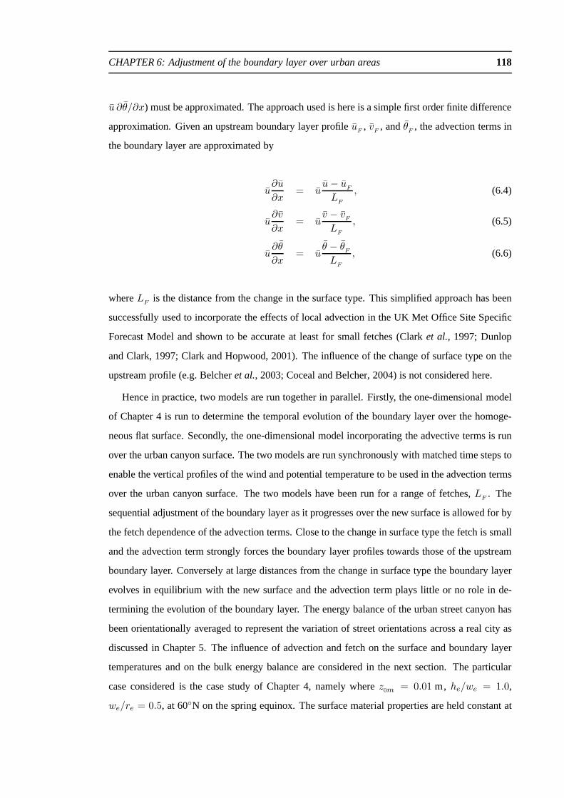
CHAPTER 6: Adjustment of the boundary layer over urban areas 118
u ∂θ/∂x) must be approximated. The approach used is here is a simple first order finite difference
approximation. Given an upstream boundary layer profileuF
, vF
, andθF
, the advection terms in
the boundary layer are approximated by
u∂u
∂x= u
u− uF
LF
, (6.4)
u∂v
∂x= u
v − vF
LF
, (6.5)
u∂θ
∂x= u
θ − θF
LF
, (6.6)
whereLF is the distance from the change in the surface type. This simplified approach has been
successfully used to incorporate the effects of local advection in the UK Met Office Site Specific
Forecast Model and shown to be accurate at least for small fetches (Clarket al., 1997; Dunlop
and Clark, 1997; Clark and Hopwood, 2001). The influence of the change of surface type on the
upstream profile (e.g. Belcheret al., 2003; Coceal and Belcher, 2004) is not considered here.
Hence in practice, two models are run together in parallel. Firstly, the one-dimensional model
of Chapter 4 is run to determine the temporal evolution of theboundary layer over the homoge-
neous flat surface. Secondly, the one-dimensional model incorporating the advective terms is run
over the urban canyon surface. The two models are run synchronously with matched time steps to
enable the vertical profiles of the wind and potential temperature to be used in the advection terms
over the urban canyon surface. The two models have been run for a range of fetches,LF
. The
sequential adjustment of the boundary layer as it progresses over the new surface is allowed for by
the fetch dependence of the advection terms. Close to the change in surface type the fetch is small
and the advection term strongly forces the boundary layer profiles towards those of the upstream
boundary layer. Conversely at large distances from the change in surface type the boundary layer
evolves in equilibrium with the new surface and the advection term plays little or no role in de-
termining the evolution of the boundary layer. The energy balance of the urban street canyon has
been orientationally averaged to represent the variation of street orientations across a real city as
discussed in Chapter 5. The influence of advection and fetch on the surface and boundary layer
temperatures and on the bulk energy balance are considered in the next section. The particular
case considered is the case study of Chapter 4, namely wherez0m = 0.01 m, he/we = 1.0,
we/re = 0.5, at 60N on the spring equinox. The surface material properties areheld constant at

CHAPTER 6: Adjustment of the boundary layer over urban areas 119
k = 0.75 WK−1m−1 andcs = 1.5 × 10⁶ JK−1m−3.
6.3 Impacts of advection
A number of processes occur as a boundary layer passes from one surface type to another. Both
a dynamical adjustment due to a change in the roughness length and the displacement height and
a thermodynamical adjustment due to a change in the energy balance can occur with distance
from the change in surface type. The quantitative impacts ofthese processes, and the sequential
adjustment and feedback through the boundary layer, on the bulk energy balance of the urban street
canyon and on the boundary layer potential temperatures allows an assessment of the importance
of advection.
6.3.1 Diurnal cycle of temperatures
The diurnal pattern of the surface and near-surface air temperature is affected by the adjustment
process within the boundary layer. Figure 6.3(a) shows the diurnal pattern of the street surface
temperature and Figure 6.3(b) the diurnal pattern of the 15 mpotential temperature for five cases
considered. The thin solid line shows the profile for the upstream flat surface and is that given
in Section 4.5. The thick solid line shows the profile for the equilibrated urban canyon surface
(i.e. no advection term). The dash-dotted, dotted and dashed lines show the profiles for the urban
canyon surface at distances of 100 m, 1,000 m and 10,000 m downstream of the surface change
respectively.
a)0 3 6 9 12 15 18 21 24 27 30 33 36
275
280
285
290
295
300
local solar time (hrs)
stre
et s
urfa
ce te
mpe
ratu
re (
K)
b)0 3 6 9 12 15 18 21 24 27 30 33 36
275
280
285
290
295
300
local solar time (hrs)
15m
pot
entia
l tem
pera
ture
(K
)
Figure 6.3: Diurnal temperature profiles from the coupled model incorporating advection. (a) street sur-face temperature; (b) 15 m potential temperature. Thin solid line, upstream profile; thick solid line, fullyadjusted profile; dash-dotted line, profile after 100 m adjustment to the new surface; dotted line, profileafter 1,000 m adjustment to the new surface; dash-dotted line, profile after 10,000 m adjustment to the newsurface.
The effects of urbanisation on the surface and near-surfacetemperatures are mainly felt during
the night time. The surface temperature is shown to adjust tothe local canyon morphology after

CHAPTER 6: Adjustment of the boundary layer over urban areas 120
even a very short fetch. Only 20–25% of the difference between the two equilibrated profiles
occurs between fetches of 100 m and 10,000 m fetch showing that the adjustment process is of
secondary importance when considering the street surface temperature. The physical mechanism
dominating the surface temperature change is the shape factor effect on the net radiation. This
process depends only on the local geometry and therefore occurs immediately at the change in
surface type. The large reduction in the maximum street surface temperature (as compared to
Figure 4.8(a)) is due to the orientational averaging performed on the canyon energy balance.
The 15 m potential temperature shows a different dependencewith fetch as seen in Figure
6.3(b). By day, the differences are small due to the large depth over which differences in the sur-
face forcing are spread in unstable conditions. By night, however, the 15 m potential temperature
shows little change at short fetches unlike the street surface temperature. Indeed, even at a fetch of
10,000 m the 15 m potential temperature still does not approach that of the equilibrated boundary
layer! Only approximately 60% of the difference between theboundary layer profiles over the flat
and canyon surfaces occurs by a fetch of 10,000 m. The boundary layer potential temperature is
dependent on the bulk surface energy balance and on the advection of the upstream profile. These
processes require time to alter the boundary layer profile which introduces a fetch dependence on
the urban impact modelled. The adjustment process also affects the surface with 25% of the urban
impact on the surface temperature occuring in the adjustment process.
6.3.2 Diurnal cycle of the energy balance
Changes in the boundary layer potential temperature profiles are caused by changes in the bulk
surface energy balance. The adjustment of the boundary layer can therefore also be observed in
the bulk energy balance. Figure 6.4 shows the diurnal profiles of the bulk sensible heat flux from
the five cases considered earlier. The differences between the profiles are small, as the radia-
tive forcing and material properties are the same in all cases, but there are important qualitative
differences.
Negative sensible heat fluxes occur around dusk in all five cases. The strong radiative cooling
of the surface is sufficient to produce stable boundary layers. The surface cooling of the upstream
surface is stronger than that of the canyon surface (the shape factor effect) and, over time with at-
mospheric mixing, is sufficient to cool the upstream near-surface air temperature below the surface
temperature of the canyon surfaces. The advection of this cool near-surface air over the warmer

CHAPTER 6: Adjustment of the boundary layer over urban areas 121
0 3 6 9 12 15 18 21 24 27 30 33 36−50
0
50
100
150
200
local solar time (hrs)
bulk
sen
sibl
e he
at fl
ux (
W m
−2 )
Figure 6.4: Diurnal profiles of the bulk sensible heat flux from the coupled model incorporating advec-tion. Thin solid line, upstream profile; thick solid line, fully adjusted profile; dash-dotted line, profileafter 100 m adjustment to the new surface; dotted line, profile after 1,000 m adjustment to the new surface;dashed line, profile after 10,000 m adjustment to the new surface.
canyon facets then triggers positive nocturnal sensible heat fluxes from the canyon surfaces. A
positive sensible heat flux acts to cool the surface and warm the boundary layer reducing the mag-
nitude of the sensible heat flux with distance travelled. Therefore the region that releases positive
sensible heat flux is restricted to the region of the urban area in the vicinity of the surface change
(Figure 6.5).
6.3.3 Adjustment with fetch
There are a range of length scales on which the atmosphere andsurface variables respond to a
change in the surface type. Knowledge of these length scalesis needed when deciding how best to
incorporate the adjustment process into numerical weatherprediction models. For instance, a rapid
adjustment can be incorporated by simply changing the parameter value(s) responsible. However,
for a longer adjustment, where the both mean and final effectsmay be needed, more care needs to
be taken. Figure 6.5 shows transects of boundary layer properties across the homogeneous urban
area at midnight (thick lines) and at dawn (thin lines) and shows the length scales of adjustment.
Figure 6.5(a) shows transects of the street surface temperature (solid lines) and 15 m potential
temperature (dash-dotted lines) with distance from the change in surface type. For reference,
the upwind surface temperature at midnight is 277 K and at dawn is 273 K. The upwind
15 m potential temperatures take the same value as at zero fetch. There are two adjustment length
scales influencing the change in surface temperature with fetch. Firstly, there is the short (m’s to
instantaneous) adjustment due to the shape factor effect onthe net radiation. Secondly, a longer
length scale (10’s km) relates to the adjustment of the boundary layer as the wind, turbulence and

CHAPTER 6: Adjustment of the boundary layer over urban areas 122
a)0 2000 4000 6000 8000 10000
276
278
280
282
284
286
distance from surface change (m)te
mpe
ratu
re (
K)
b)0 2000 4000 6000 8000 10000
1.5
2
2.5
3
3.5
distance from surface change (m)
15m
win
d sp
eed
(m s
−1 )
c)0 2000 4000 6000 8000 10000
−20
−10
0
10
20
distance from surface change (m)
bulk
sen
sibl
e he
at fl
ux (
W m
−2 )
Figure 6.5: Transect of atmospheric variables from the change in surface type. Thick lines, transects atmidnight; thin lines, transects at dawn 6 hours later. (a) solid line, street surface temperature; dash-dottedline, 15 m potential temperature; (b) 15 m wind speed; (c) bulk sensible heat flux.
potential temperature profiles adapt to the changing surface energy balance. Within the boundary
layer this second length scale dominates.
Figure 6.5(b) shows the transect of the 15 m wind speed. The 15m wind speed is influenced by
two length scales. The first, dominant, length scale (1–2 km)relates to the adjustment to the new
bulk roughness length and displacement height. The second length scale relates to the dependence
of the mean wind profile on the stability of the boundary layerand hence to the changing surface
energy balance.
The surface energy balance is influenced by both the wind speed and the boundary layer po-
tential temperature. Therefore all the length scales for adjustment are present in the transect of the
bulk sensible heat flux (Figure 6.5(c)). Note that although the street surface temperature is greater
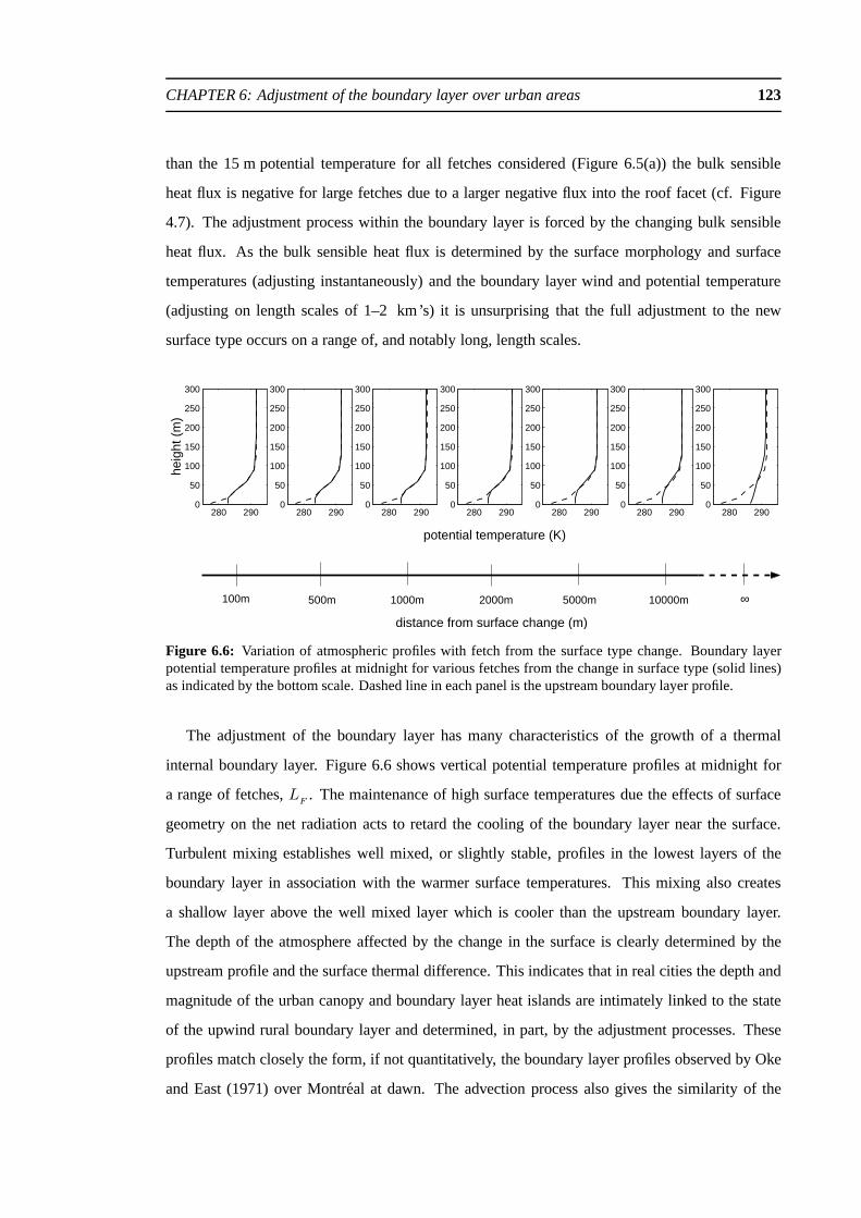
CHAPTER 6: Adjustment of the boundary layer over urban areas 123
than the 15 m potential temperature for all fetches considered (Figure 6.5(a)) the bulk sensible
heat flux is negative for large fetches due to a larger negative flux into the roof facet (cf. Figure
4.7). The adjustment process within the boundary layer is forced by the changing bulk sensible
heat flux. As the bulk sensible heat flux is determined by the surface morphology and surface
temperatures (adjusting instantaneously) and the boundary layer wind and potential temperature
(adjusting on length scales of 1–2 km’s) it is unsurprising that the full adjustment to the new
surface type occurs on a range of, and notably long, length scales.
280 2900
50
100
150
200
250
300
heig
ht (
m)
280 2900
50
100
150
200
250
300
280 2900
50
100
150
200
250
300
280 2900
50
100
150
200
250
300
280 2900
50
100
150
200
250
300
280 2900
50
100
150
200
250
300
280 2900
50
100
150
200
250
300
potential temperature (K)
100m 500m 1000m 2000m 5000m 10000m ∞
distance from surface change (m)
Figure 6.6: Variation of atmospheric profiles with fetch from the surface type change. Boundary layerpotential temperature profiles at midnight for various fetches from the change in surface type (solid lines)as indicated by the bottom scale. Dashed line in each panel isthe upstream boundary layer profile.
The adjustment of the boundary layer has many characteristics of the growth of a thermal
internal boundary layer. Figure 6.6 shows vertical potential temperature profiles at midnight for
a range of fetches,LF
. The maintenance of high surface temperatures due the effects of surface
geometry on the net radiation acts to retard the cooling of the boundary layer near the surface.
Turbulent mixing establishes well mixed, or slightly stable, profiles in the lowest layers of the
boundary layer in association with the warmer surface temperatures. This mixing also creates
a shallow layer above the well mixed layer which is cooler than the upstream boundary layer.
The depth of the atmosphere affected by the change in the surface is clearly determined by the
upstream profile and the surface thermal difference. This indicates that in real cities the depth and
magnitude of the urban canopy and boundary layer heat islands are intimately linked to the state
of the upwind rural boundary layer and determined, in part, by the adjustment processes. These
profiles match closely the form, if not quantitatively, the boundary layer profiles observed by Oke
and East (1971) over Montreal at dawn. The advection process also gives the similarity of the

CHAPTER 6: Adjustment of the boundary layer over urban areas 124
urban and rural boundary layer profiles at altitude (Figure 6.6), which was a weakness in the one
dimensional model.
The upstream boundary layer profiles in real life will be those of the surrounding rural coun-
tryside and not that of a flat, smooth, dry surface. Moisture plays a particularly important role
in determining the energy balance and boundary layer profiles in rural areas (e.g. McNaughton
and Spriggs, 1986) and will therefore impact on the adjustment of the boundary layer to an urban
surface. In rural areas moisture acts to decrease the surface sensible heat flux as well as to de-
crease the surface and boundary layer temperatures during the day. The advection of this cooler
boundary layer over an urban surface will result in larger values of the bulk sensible heat flux by
day and night, reduced daytime temperatures and a greater fetch of urban surface generating pos-
itive nocturnal sensible heat fluxes when compared to the drysimulations. For instance, an order
of magnitude estimate of the impact of incorporating a latent heat flux equal to the sensible heat
flux by day and zero at night (a Bowen ratio equal to 1), indicates that this would have the effect
of extending the region of positive nocturnal sensible heatfluxes out to 5 km from the change in
surface type at dawn. Moisture will also affect the timing ofthe maximum heat island intensity,
which is a weakness in the one dimensional model, through both its direct influence on the refer-
ence rural boundary layer and also indirectly through the advection process. A full investigation
of the impacts of moisture on the energy balance of urban areas and on the adjustment process
remains for future work.
6.4 Summary and implications
This chapter investigated the adjustment of the boundary layer and surface energy balance to an
urban area. The advective terms in the boundary layer were incorporated into the coupled canyon
energy balance and boundary layer model using a method involving a relaxation to the upstream
boundary layer. Coupling the boundary layer modelled over aflat surface to the boundary layer
over the canyon energy balance allowed the adjustment of theboundary layer and surface energy
balance to the effects of surface morphology to be investigated.
Adjustment was seen to be a key process affecting the surfaceenergy balance, as well as the
boundary layer dynamics and thermodynamics of the urban area. At the surface, the urban im-
pact on surface temperature is felt almost immediately through the shape factor effect. In the
atmospheric boundary layer the urban impact is felt entirely through the adjustment process. The
CHAPTER 6: Adjustment of the boundary layer over urban areas 125
interactions between the boundary layer and the energy balance act to provide a further 25% of
the urban impact on the surface temperature.
The adjustment processes occur on a range of spatial scales and through a range of physi-
cal mechanisms. The shape factor effect on the net radiationand the dynamic adjustment to the
increased roughness and displacement occur on short lengthscales. The thermodynamic adjust-
ment, accomplished through the interactions of the boundary layer and the energy balance, occurs
on longer length scales. This combined adjustment process is found here to require over 10 km of
uniform surface to become fully equilibrated. A key result is that the adjustment process can allow
the generation of positive nocturnal sensible heat fluxes.
There are a range of implications of this simple study. This work has shown that neutral
nocturnal boundary layers can be explained by the adjustment process without the need to invoke
large anthropogenic heat fluxes. The adjustment process is unlikely to equilibrate in real life as
urban areas typically vary their characteristics on much shorter length scales than those shown to
be required for full adjustment. Successive adjustments can then realise large regions of urban
areas which can release positive nocturnal sensible heat fluxes.
Adjustment on length scales shorter than the grid spacing isdifficult to incorporate into numer-
ical weather models. Together with the long length scale required for thermodynamic adjustment
this poses problem in determining the morphological properties representative of an urban area.
For instance, suppose that within one grid box of a numericalweather prediction model there are
two successive changes in urban surface. The adjustment process could then generate two regions
of the urban area with positive nocturnal sensible heat fluxes and thus give a positive heat flux for
the grid point. With only one representative set of values for the morphological properties of the
urban surface, the numerical weather prediction model would be unable to incorporate the succes-
sive adjustments without increasing the resolution. Negative nocturnal sensible heat fluxes could
then be predicted for the grid point even when incorporatingthe urban energy balance. Finally, the
adjustment process will, in some way, also determine whether each individual urban area is large
enough that it needs to be incorporated into numerical weather prediction models.
Advection and the accompanying adjustment processes within the boundary layer have been
shown to play an important role in the simple case consideredhere. It is suggested that advection
plays a key role in determining the impact of real urban areason the local surface energy balance
and boundary layer.

CHAPTER SEVEN
Conclusions
7.1 Summary of thesis
Urban areas pose a complex problem for the atmospheric scientist because of the complexity of
the surface and the turbulent nature of the planetary boundary layer. Despite large differences in
building configuration, for example, between individual urban areas, there are common themes in
the observed modifications of the local climate by urban areas. Urban areas are generally warmer,
less windy and drier in a relative sense than their rural surroundings, with these differences varying
on all time and space scales. The large differences between urban areas make the understanding
and prediction of the modifications to the local climate by anurban area difficult primarily because
there are a large number of plausible causes.
The characteristic common to all urban areas are buildings.Buildings impose two properties
on the surface of an urban area. Firstly, the total surface area is increased from that of a horizontal
surface. Secondly, there is necessarily a change in thegeometryof the surface to accommodate
the increase in total surface area. Together these properties comprise themorphologyof the urban
surface. It is suggested that a cause of the modifications to the local climate by urban areas results
from the combination of the effects of surface morphology. However, the full impacts of just the
surface morphology on the urban climate had not been investigated thoroughly before this study.
Urban areas are surface features and so impose their modifications of the local climate by
altering the surface energy balance and wind stress. In doing so the profiles of wind, temperature
and humidity in the atmospheric boundary layer are altered.As the surface energy balance itself
is determined in part by these profiles, the surface and boundary layer form one coupled system.
126
CHAPTER 7: Conclusions 127
The aims of this work were therefore:
To investigate thoroughly the influence of surface morphology on the individual terms of
the surface energy balance of, and boundary layer, over urban areas.
To establish which of the observed urban modifications of thelocal climate can be explained
by the combined effects of surface morphology and to proposealternative physical mecha-
nisms for those that cannot, and finally
to establish a method to incorporate urban areas, notably the effects of surface morphology,
into numerical weather prediction models.
To address these aims a generic unit of the urban surface, a dry urban street canyon, was used
as the basis for a model of the surface energy balance of an urban area. The energy balance of, and
boundary layer over, flat surfaces were compared with those over urban street canyon surfaces to
investigate the influence of surface morphology on the individual facet-averaged and bulk energy
balances, on the surface temperatures and on the profiles of wind and potential temperature in
the boundary layer. A range of analytic, experimental and numerical methods were used in this
investigation.
The first aim of the work was addressed in Chapters 2 and 3. Chapter 2 and Appendix A
considered the effects of canyon geometry on the radiative fluxes. A matrix method (Sparrow
and Cess, 1970) to calculate the facet-averaged net radiative flux densities for a street canyon,
incorporating multiple reflections of radiation, was presented. This method was compared to two
approximate, and commonly used, methods incorporating onereflection of radiation (e.g. Johnson
et al., 1991) or no reflections (e.g. Noilhan, 1981) across a wide range of canyon geometries. The
effects of canyon geometry on the flux densities and bulk radiation balance were considered as
well as the validity of the two approximate methods.
Chapter 3 considered the turbulent transfer within an urbanstreet canyon. A model for the
facet-averaged turbulent flux of a scalar, such as heat, fromeach facet of an urban street canyon
was presented. The influence of canyon morphology on the turbulence within the boundary layer
above the buildings and within the street canyon was incorporated into the model. Model predic-
tions compared well with observations from Barlow and Belcher (2002) and Barlowet al. (2004)
and were used to give insight into the important physical processes responsible for the turbulent
transfer close to the surface of an urban area. The morphological dependence of the ground heat

CHAPTER 7: Conclusions 128
flux in an urban area is dependent solely on the surface area and surface temperature variation so
was not considered in detail.
Results from Chapters 2 and 3 were used to formulate the urbanstreet canyon energy balance
as presented in Chapter 4. The canyon energy balance model was coupled to a one dimensional
boundary layer model (Buschet al., 1976) to allow the interactions between the surface and bound-
ary layer that are present in reality (e.g. Brubaker and Entekhabi, 1996; Raupach, 2001) to occur.
This coupled model was then used to investigate the dependence of the average energy balances
of the canyon facets, of thebulk energy balancefor the entire canyon unit and of the boundary
layer state to surface morphology. Additionally the model was used to determine qualitatively
which observations of the urban modification of climate can be explained by surface morphology
alone. Chapter 5 addressed the final aim of identifying a method to incorporate urban areas into
numerical weather prediction models. The full four facet canyon energy balance was averaged in
two ways (two facets - canyon and roof, and only one facet) to assess the degree of complexity
needed to capture the effects of the urban street canyon.
Chapter 4 illustrated that some key features of the urban modification of climate, notably posi-
tive nocturnal sensible heat fluxes, cannot be explained solely by the effects of surface morphology
on the bulk energy balance and boundary layer. Chapter 6 investigated possible causes for this fea-
ture, notably the advection of a rural boundary layer over anurban area.
Throughout this work the individual results are related to two concurrent themes - these con-
clusions will address these themes in turn. Firstly, the increase in surface area and the geometry
of the surface influences all parts of the energy balance-boundary layer system. Net changes often
result as the residual between opposing changes imposed by the two properties. Secondly, the sur-
face energy balance and boundary layer form one system; one cannot be done without the other.
Changes in one part of the system may relate to physical processes acting on a separate part.
7.2 Conclusions
Surface morphology influences the urban energy balance and urban boundary layer by increasing
the total area of the surface available for energy exchange and by deforming the surface. The
increased total surface area of an urban area reduces the magnitude of the average flux densities of
all terms in the energy balance from the horizontal and vertical surfaces given the same external
radiative forcing (Sections 2.5, 3.9, 4.4 and 4.8). The diurnal temperature variation at the surface
CHAPTER 7: Conclusions 129
and near surface is therefore also reduced. However, the increase in total surface area acts to
increase the bulk flux of longwave radiation away from the topof the convoluted surface with a
corresponding decrease in the bulk sensible and bulk groundheat fluxes (Section 4.4).
Accompanying these changes due to surface area is a range of effects imposed by the geometry
of the surface. Firstly, given the same atmospheric and surface temperatures, the bulk radiative
and bulk sensible heat fluxes are increased in magnitude. This is despite the flux densities on the
individual facets decreasing. This therefore illustratesthe competing influences of an increased
surface area and surface geometry. Secondly, the incoming longwave radiation for the canyon
facets partly originates from the other facets and not the sky. This shape factor effectreduces
the magnitude of the net longwave radiative flux densities and acts to offset (usually positively)
the mean surface temperature. Thirdly, shadowing and the inclination of surfaces results in a
non-uniform distribution of shortwave radiation onto the canyon facets. Finally, surface geometry
acts to increase the roughness length and displacement height representative of the mean wind
in the boundary layer over an urban area which is correspondingly reduced. These processes,
notably the reduction in the turbulent flux densities, alterthe partitioning of energy into its various
forms compared to a horizontal surface and act to change the phases of the fluxes. A roughened
surface without surface geometry is unable to reproduce these effects and can give opposite results
(Section 4.5).
The boundary layer plays a key role in determining the modifications to the local climate by
urban areas. By day, when the differences in the energy balance (i.e. the bulk sensible heat flux)
between different cases are large, the increased depth of the boundary layer acts to spread the dif-
ference in the surface forcing in the vertical. This, together with the offset in surface temperature
due to the shape factor effect, results in small thermal differences in the boundary layer by day.
Conversely by night, when the differences in the bulk sensible heat flux between cases are small,
the reduced depth of the stable boundary layer allows large thermal differences. This process,
in conjunction with the offset in surface temperature due tothe shape factor effect, means that
the observed diurnal cycle of the surface and near-surface nocturnal urban heat islands (e.g. Oke,
1987) can be explained in terms of surface morphology alone.
Stability effects within the boundary layer act to reinforce the differences between the bound-
ary layers over an urban canyon and flat surface, particularly during the night. The increased
roughness and mixing due to geometry act to increase the efficiency of the turbulent transport
of heat between the atmosphere and the surface. This mixes the nocturnal atmospheric cooling

CHAPTER 7: Conclusions 130
through a greater depth of the boundary layer. This in turn reduces the stability of the nocturnal
urban boundary layer. A reduction in the stability of the boundary layer increases the turbulent
mixing which reinforces the nocturnal thermal differences. The combined effects of surface mor-
phology therefore act to produce warmer, deeper and less stable nocturnal boundary layers over
urban areas.
The variation of these effects with canyon geometry qualitatively explains some of the spatial
variation in the urban modifications to the local climate. With increasing urbanisation (increasing
canyon aspect ratio) the near-surface nocturnal thermal anomalies increase in magnitude as seen in
spatial maps of the mean urban heat island (Oke, 1987). As thecanyon aspect ratio is increased the
canyon bulk energy balance is altered in two ways. Firstly the bulk sensible heat flux is decreased
in magnitude with its peak value and the transition to stableconditions delayed (as observed by
Grimmond and Oke (2002)). Secondly the bulk ground heat flux is increased in magnitude with
its peak value occuring earlier during the day (as observed by Cleugh and Oke (1986)).
The coupled nature of the surface energy balance and boundary layer is highlighted further
when explaining positive nocturnal sensible heat fluxes. The advection of a stable (rural) boundary
layer over an urban surface was shown (Chapter 6) to be a plausible cause for this characteristic
feature of urban areas. A one dimensional coupled model is unable to produce positive nocturnal
sensible heat fluxes unless a mechanism is introduced to decouple the boundary layer and surface
temperatures. Including the advection process in the boundary layer provides this mechanism and
enables positive nocturnal sensible heat fluxes to be generated. The urban boundary layer heat
island was seen to take the form of a thermal internal boundary layer (Section 6.3; Oke and East,
1971). When advection is included in the model the surface thermal anomalies are also altered:
Only at a fetch of some 20 km are the thermal anomalies equal tothe one dimensional simulations.
The variation in spatial patterns of the urban heat island (e.g. Graveset al., 2001) can then be
interpreted as the variability due to advection of different adjusting boundary layers over the same
urban surface. The energy balance, dynamic and thermodynamic impacts of urban areas should
therefore be investigated using a coupled boundary layer-surface energy balance model where the
full effects of surface morphology have been incorporated.Other features of urban areas (e.g.
building material properties) can influence the urban modification of the local climate but play a
secondary role.
The geometry of the urban surface allows the energy balancesof the different building facets to
interact directly. This is a property of the urban surface for which the surface exchange schemes of

CHAPTER 7: Conclusions 131
most operational weather prediction models are not configured. However, providing the impacts
of surface morphology on the radiation, bulk roughness length, bulk displacement height and
turbulent transport are kept, the bulk energy balance from the four-facet urban street canyon can
be successfully approximated using two facets (Section 5.3). These two facets are an unchanged
roof facet and a canyon facet which is the average of the street and two walls weighted by surface
area. The bulk energy urban street canyon cannot be successfully approximated across the full
range of urban morphologies using only one facet due, primarily to the non-uniformity of the
direct solar radiation.
There are a number of caveats to attach to these results. Firstly, the assumption that the energy
balance of urban areas can be represented as that from a series of urban street canyons requires
investigation. Care needs to be taken when extrapolating from the street canyon studies to real
urban areas (see Section 3.7). Massonet al. (2002) has shown that an energy balance model based
on an urban street canyon gives reasonable predictions of the observed energy balance in a range
of locations. However, this work forces the energy balance with observations and therefore does
not allow the coupled nature of the system to develop. However, the processes highlighted here
(surface area, geometry and the coupled system) apply qualitatively to any array of buildings.
Secondly, urban areas cannot be considered to be dry. Moisture was ignored in this study
to reduce the number of processes. Therefore comparisons between the energy balance of, and
boundary layer over, the flat and urban canyon surfaces may not be indicative of the differences
between urban and rural sites. Moisture is known to play an important role in the energy balance
of an urban area during and after rain events (Landsberg, 1981) and there is increasing interest in
the role of dew fall in urban areas (e.g. Richards and Oke, 2002). Additionally, moisture will play
a significant role in determining the upstream boundary layer when considering the adjustment
process (Chapter 6). The coupled nature of the energy balance and boundary layer implies that
this will affect, quantitatively at least, the results concerning the generation of positive nocturnal
sensible heat fluxes.
Finally, the anthropogenic heat flux in urban areas althoughcommonly small may be sufficient
to explain some observations of urban areas. Anthropogenicforcing can influence the surface
energy balance directly (e.g. the maintenance of internal building temperatures as done here) or
indirectly (e.g. traffic induced turbulence (Raoet al., 2002), or heat emissions directly into the
boundary layer (Kannariet al., 2003; Sailoret al., 2003)). These forcings may be important in
specific cases (e.g. Ichinoseet al., 1999; Spronken-Smithet al., 2003) and in explaining the timing

CHAPTER 7: Conclusions 132
of transitions between stable and unstable conditions.
7.3 Impact on the wider picture
This work complements and adds to a range of existing work. This work confirms the conclusions
from the work of Okeet al. (1991) that the principal causes for the urban modification to the
local climate arise through surface morphology, with the building material properties (notably the
thermal admittance) playing the second role. This work shows that these conclusions hold when
the turbulent fluxes and the interactions between the boundary layer and surface energy balance
are included.
Other urban energy balance models exist (e.g. Masson, 2000;Kusakaet al., 2001; Grimmond
and Oke, 2002; Martilliet al., 2002; Vuet al., 2002) which do not incorporate the dependence of
the energy balance on surface morphology to the extent of this study. This work has shown the
impact that a few additional processes can have on the model predictions, notably the inclusion
of multiple reflections of radiation and the inclusion of turbulent fluxes which depend on the
surface morphology and the overlying boundary layer characteristics. While the impact that these
processes would have on these models is not immediately obvious, their impact on this work
is significant and suggests that the properties of the coupled system (the balance between the
increased surface area and geometry on the bulk fluxes for example) should be present in any
model of the energy balance of an urban area.
Realisation of the importance of the boundary layer over theurban area in determining the
energy balance and the temperature profiles is relatively new to this field. The boundary layer was
seen to be a controlling influence on the turbulent fluxes and therefore the surface and near-surface
temperatures. Catonet al. (2003) observed a similar dependence on the boundary layer turbulent
intensity when considering the ventilation of pollutants from a street canyon. The adjustment of
the boundary layer as it progresses over an urban area, and inparticular the generation of positive
nocturnal sensible heat fluxes, is of particular importancein a variety of applications. Future
work into the energy balance of urban areas must consider theenergy balance and boundary layer
together especially when considering the sensitivities ofthe energy balance.
This work as a whole has confirmed the need for models of the energy balance of an urban area
to incorporate surface morphology. Most of the bulk impactsof urban areas on the local climate
can be captured using relatively simple methods provided the full range of physical processes

CHAPTER 7: Conclusions 133
resulting from surface morphology are incorporated in boththe energy balance and the boundary
layer.
7.4 Future work
This work has developed understanding of the mechanisms acting which determine many of the
modifications to the local climate made by urban areas. However, there are a number of avenues
which remain to be investigated or which have opened due to this work.
Application of the naphthalene sublimation technique for measuring the facet-averaged turbu-
lent fluxes can be extended in two ways. Firstly, alternativetwo dimensional geometries could be
used to validate the model developed in Chapter 3 and for alternative canyon orientations. Sec-
ondly, the technique could be applied to a three dimensionalarray of buildings. This second use
would allow an assessment of the differences between two andthree dimensional geometries and
indicate whether the urban street canyon should be used as a generic unit of an urban area. This
broader aim could also be investigated by extending the radiative transfer model (Chapter 2) to
three dimensions and comparing the results to the existing two dimensional calculations.
Moisture in the urban energy balance is a key issue to address. In an operational setting, where
representative surface types for the grid points are required, this could be achieved by allowing a
dry urban surface but reducing the fractional area occupiedby the urban surface surrounding each
grid point. This method may not, however, succeed during andafter rain events. An alternative
method is to incorporate a shallow pond model on the street and roof facets as part of the street
canyon energy balance.
The specification of input parameters for real urban areas will require care. Using the urban
street canyon as the generic unit of the urban surface implies that the geometric ratioshe/we and
we/re be related in some fashion to the real urban morphology. The surface roughness length,
displacement height, radiative fluxes and turbulent fluxes all depend on the characteristic ratios in
different non-linear ways. There is therefore a difficulty in the specification of the urban canyon
parameters which preserves all of these properties of urbanareas. A related problem is that within
numerical weather prediction models these input parameters will be representative of the area sur-
rounding the grid point. However, in real urban areas the characteristic ratios vary on length scales
smaller than the numerical weather prediction models’ grid-point separation. It is not immediately
obvious how these input parameters should be chosen in orderto preserve the mean bulk energy

CHAPTER : Conclusions 134
balance.
The individual terms of the energy balance model developed here have been compared to either
existing methods or new data. However, the full energy balance model remains to be validated.
Such a validation would require the careful consideration of a number of points. For instance, can
observations be made of the modelled variables e.g. facet-averaged energy balances? Additionally
should one attempt to validate the entire boundary layer-surface energy balance model or just the
surface component?
A final section of future work is the implementation of an urban energy balance into an opera-
tional numerical weather prediction model. Chapter 4 illustrated the properties that such a scheme
should possess and Chapter 5 a possible method to do this. Once implemented, and questions over
the input parameters have been overcome, several questionscan be addressed. Firstly, is there an
improvement of the forecast of local properties, e.g. the street surface temperature? Secondly, is
there an improvement in the forecast at larger (city or regional) scales? Finally, is there evidence
of urban areas influencing mesoscale or synoptic scale weather features? A related but separate
issue is the relation of this work to canopy models. These models have been applied to incorpo-
rate vegetation and urban areas (e.g. Best, 1998a) into numerical weather prediction models. This
approach has been successfully used to predict the spatially averaged mean winds through urban
areas (Belcheret al., 2003; Coceal and Belcher, 2004) and progress has been made towards incor-
porating surface morphology into the energy balance for an urban canopy (e.g. Vuet al., 2002).
A common method to deal with both the dynamic and thermodynamic aspects of the influence of
any surface type on the boundary layer within numerical weather prediction models may therefore
be possible.

APPENDIX A
Solar radiation in an urban street canyon
Solar radiation on arbitrary surfaces
The wavelength-integrated shortwave radiative flux density, or insolation, received at the top of the
atmosphere,Ktoa, is primarily determined by the position of the Earth relative to the Sun and solar
activity. The insolation received at the Earth’s surface additionally depends on the latitude, time of
day, elevation and orientation of the surface as well as radiative processes within the atmosphere.
Both the direct and diffuse components of the solar radiative flux density for an arbitrarily inclined
and oriented surface are needed to provide a solar forcing for the surface energy balances described
in Chapter 4.
i
θi
m
A θi
A
Figure A.1: Relative surface area for a surface oriented to a solar ray.
Consider first the geometric dependency of the direct solar radiative flux density that results
from the variation in the direction of the sun’s rays. Define the solar incidence angle,θi, to
be the angle between the normal to the surface and the sun’s rays and denote the direct solar
radiative flux density onto a surface normal to the sun’s raysasK⊥ (i.e. incorporating atmospheric
radiative effects but no geometric effects) as shown in Figure A.1. For a horizontal surface the solar
incidence angle is equivalent to the solar zenith angle,θ. As the surface need not be normal to the
135

APPENDIX A: Solar radiation in an urban street canyon 136
Stoa sin ψ
m
ψ ζvertical cross sectiona)
z
Stoacos ψ cos α
cos ψ αsin
ζ
E
N
α
plan viewb)
Figure A.2: Schematic of the unit vector aligned with a solar ray; (a) elevation; (b) orientation.
sun’s rays the surface area,Ai, onto which the solar flux impinges is increased through a geometric
factor given by
A = Ai cos θi, (A.1)
and hence the flux density onto the surface,Ksf , is decreased to ensure conservation of energy to
Ksf = K⊥ cos θi. (A.2)
The angle between any two vectors,m andn, and hence between the normal to a plane and a
line, can be calculated using the scalar product (m ·n = |m||n| cos θi). The geometric dependency
of the direct component of the solar radiative flux density for an arbitrary surface can therefore be
determined by calculating the unit vectors of the normal to the surface and of the sun’s rays (e.g.
Owczarek, 1997). For convenience these are expressed in terms of latitude,φ, Julian day number,
dn, and time of day,h(t).
Consider first the vector describing the direction of the solar rays in a cartesian system at the
Earth’s surface aligned with thez-axis pointing vertically upwards, thex-axis pointing due east
and they-axis pointing due north. The solar rays will impinge on the surface with an elevation
angle,ψ, and azimuthal angle,α, as shown in Figure A.2.
The unit vector for the solar ray in terms of the elevation angle and azimuthal angle is:
m =
cosψ(t) sinα(t)
cosψ(t) cosα(t)
sinψ(t)
. (A.3)

APPENDIX A: Solar radiation in an urban street canyon 137
Spherical geometry (Owczarek, 1997) gives that the vectorm can be written in terms of the
latitude,φ, solar declination angle,δ, and time of day,h(t), using the following identities,
cosψ(t) sinα(t) = cos δ(dn) sinh(t), (A.4)
cosψ(t) cosα(t) = − sin δ(dn) cosφ+ cos δ(dn) sinφ cos h(t), (A.5)
sinψ(t) = sin δ(dn) sinφ+ cos δ(dn) cosφ cos h(t). (A.6)
The declination angle,δ, measures the tilt of the Earth’s rotational axis relative to its orbital
plane and can be determined from the Julian day number,dn, through Equation (A.7). The time
of day,h(t), is measured as the fraction of the day (in radians) with local noon being zero; the
relationship to the local solar time,t, is given by Equation (A.8).
δ(dn) = 0.4102 cos
[
2π(dn − 172)
365
]
, (A.7)
h(t) = 2πt− 12
24. (A.8)
The unit vector describing the direction of the solar ray is therefore
m =
cos δ sinh(t)
− sin δ cosφ+ cos δ sinφ cos h(t)
sin δ sinφ+ cos δ cosφ cos h(t)
. (A.9)
Consider now the unit vector normal to a planar surface with elevation angleβ to the horizontal
and orientation angleΩ from the north in the same cartesian coordinates as shown in Figure A.3.
The unit vector nis found to be
n =
sin β sinΩ
sin β cos Ω
cos β
. (A.10)
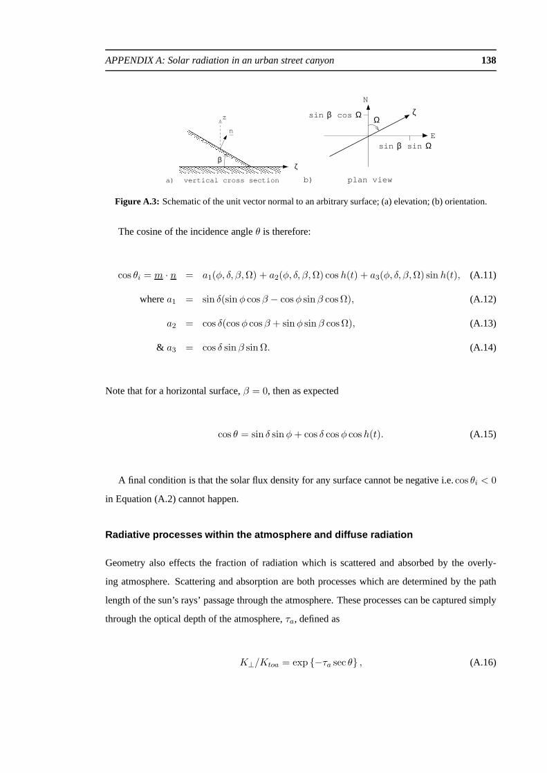
APPENDIX A: Solar radiation in an urban street canyon 138
n
βζ
vertical cross section
z
a)
cos Ωβsin
sinβ ΩsinE
ζΩ
plan view
N
b)
Figure A.3: Schematic of the unit vector normal to an arbitrary surface;(a) elevation; (b) orientation.
The cosine of the incidence angleθ is therefore:
cos θi = m · n = a1(φ, δ, β,Ω) + a2(φ, δ, β,Ω) cos h(t) + a3(φ, δ, β,Ω) sin h(t), (A.11)
wherea1 = sin δ(sin φ cos β − cosφ sin β cos Ω), (A.12)
a2 = cos δ(cos φ cos β + sinφ sin β cos Ω), (A.13)
& a3 = cos δ sin β sin Ω. (A.14)
Note that for a horizontal surface,β = 0, then as expected
cos θ = sin δ sinφ+ cos δ cosφ cos h(t). (A.15)
A final condition is that the solar flux density for any surfacecannot be negative i.e.cos θi < 0
in Equation (A.2) cannot happen.
Radiative processes within the atmosphere and diffuse radi ation
Geometry also effects the fraction of radiation which is scattered and absorbed by the overly-
ing atmosphere. Scattering and absorption are both processes which are determined by the path
length of the sun’s rays’ passage through the atmosphere. These processes can be captured simply
through the optical depth of the atmosphere,τa, defined as
K⊥/Ktoa = exp −τa sec θ , (A.16)

APPENDIX A: Solar radiation in an urban street canyon 139
where the surface receiving the radiation is at ground leveland thesec θ term represents the path
length dependence of scattering and absorption of radiation through the atmosphere. The optical
depth of the atmosphere is heavily dependent on atmosphericconstituents, cloud amounts and
their properties. For the simple purposes of determining a solar forcing the optical depth is taken
as a constant (= 0.2) throughout this work.
The diffuse solar flux density at the surface,Kdf , is determined through a complex processes
of multiple scattering and refraction. For the simple purposes of determining a forcing for the
surface energy balance, the diffuse solar radiation impinging a horizontal surface and ground level
is taken as a constant fraction (= 0.7) of the radiation whichhas been absorbed or scattered by the
atmosphere, namely
Kdf = 0.7Ktoa(1 − exp −τa sec θ). (A.17)
Shadowing
The directional nature of the direct component of the solar radiative flux density in conjunction
with a system of surfaces at different elevation angles and/or orientations can lead to the shadowing
of one surface by another. The individual facets of an urban canyon experience shadowing by
another facet at some point in the day in almost all circumstances. A shadowed facet will receive
no direct solar radiation but its full quota of diffuse radiation as described in Chapter 2. The urban
canyon energy balance model considers facet-averaged flux densities; therefore, for consistency,
a partly shadowed facet is deemed to receive a direct radiative flux density equivalent to the area-
weighted average of the shadowed and unshadowed fractions of the facet. The fraction of each
facet shadowed at any one time is a function of latitude,φ, solar declination angle,δ, canyon
aspect ratio,he/we, and canyon orientation,Ω.
Consider a cartesian set of axis where thez-axis points vertically upwards, thex-axis points
normally across the street canyon and they-axis points along the canyon. They-axis is therefore
aligned at an angleΩ to north-south. Consider first the shadow cast by a pole of heighthe placed
at the origin. The solar azimuth angle,Az, is the angle between the shadow cast on a horizontal
plane and due south as shown in Figure A.4. Sakakibara (1996)shows that the solar azimuthal
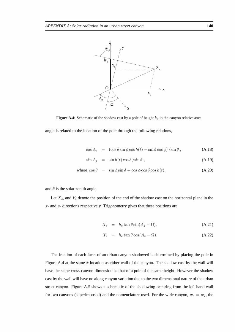
APPENDIX A: Solar radiation in an urban street canyon 140
zA
x
yz
SΩ
θ
Ο
Z
X
Ys
he
s
s
Figure A.4: Schematic of the shadow cast by a pole of heighthe in the canyon relative axes.
angle is related to the location of the pole through the following relations,
cosAz = (cos δ sinφ cos h(t) − sin δ cosφ) /sin θ , (A.18)
sinAz = sinh(t) cos δ /sin θ , (A.19)
where cos θ = sinφ sin δ + cosφ cos δ cosh(t), (A.20)
andθ is the solar zenith angle.
LetXs, andYs denote the position of the end of the shadow cast on the horizontal plane in the
x- andy- directions respectively. Trigonometry gives that these positions are,
Xs = he tan θ sin(Az − Ω), (A.21)
Ys = he tan θ cos(Az − Ω). (A.22)
The fraction of each facet of an urban canyon shadowed is determined by placing the pole in
Figure A.4 at the samex location as either wall of the canyon. The shadow cast by the wall will
have the same cross-canyon dimension as that of a pole of the same height. However the shadow
cast by the wall will have no along canyon variation due to thetwo dimensional nature of the urban
street canyon. Figure A.5 shows a schematic of the shadowingoccuring from the left hand wall
for two canyons (superimposed) and the nomenclature used. For the wide canyon,we = w2, the
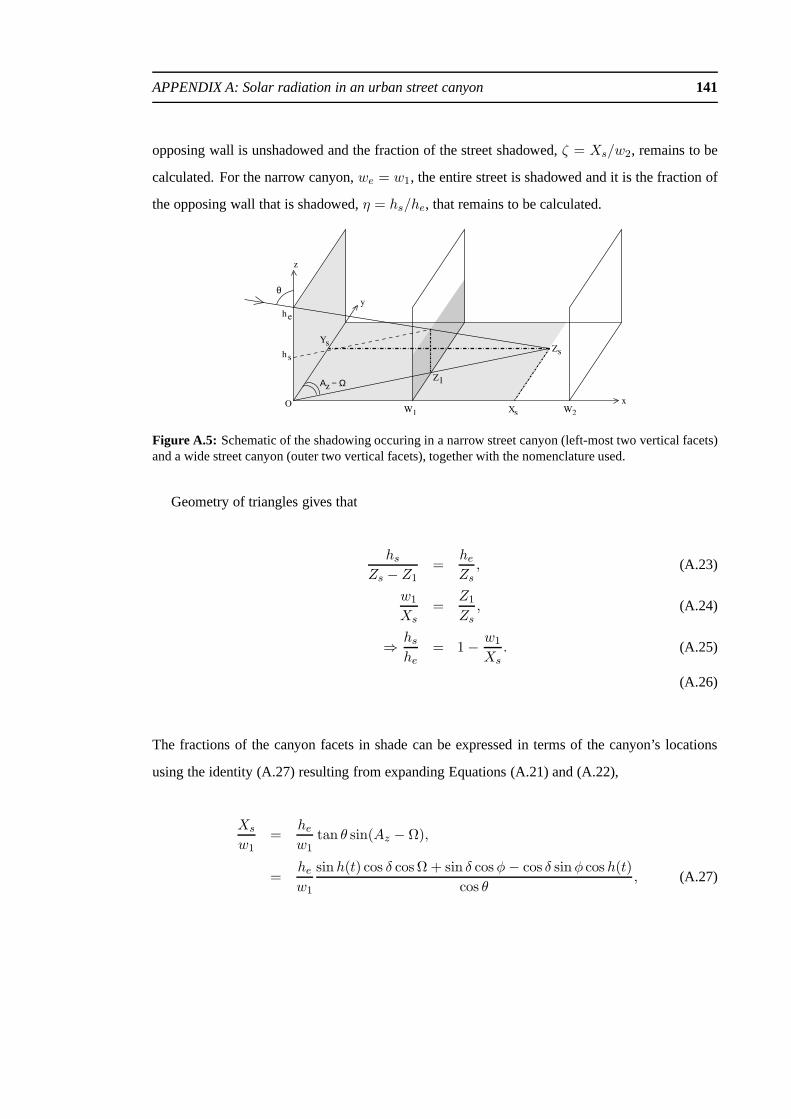
APPENDIX A: Solar radiation in an urban street canyon 141
opposing wall is unshadowed and the fraction of the street shadowed,ζ = Xs/w2, remains to be
calculated. For the narrow canyon,we = w1, the entire street is shadowed and it is the fraction of
the opposing wall that is shadowed,η = hs/he, that remains to be calculated.
W2
Αz − Ω
1W
θ
O
y
z
x
Z1
X
Z
s
s
h
Ys
e
sh
Figure A.5: Schematic of the shadowing occuring in a narrow street canyon (left-most two vertical facets)and a wide street canyon (outer two vertical facets), together with the nomenclature used.
Geometry of triangles gives that
hs
Zs − Z1=
he
Zs, (A.23)
w1
Xs=
Z1
Zs, (A.24)
⇒hs
he= 1 −
w1
Xs. (A.25)
(A.26)
The fractions of the canyon facets in shade can be expressed in terms of the canyon’s locations
using the identity (A.27) resulting from expanding Equations (A.21) and (A.22),
Xs
w1=
he
w1tan θ sin(Az − Ω),
=he
w1
sinh(t) cos δ cos Ω + sin δ cosφ− cos δ sinφ cos h(t)
cos θ, (A.27)
APPENDIX A: Solar radiation in an urban street canyon 142
The fraction of the street facet of the canyon under shadow,ζ, at any time and location is therefore,
ζ =
max[
|Xs|we, 1]
if cos θ > 0,
1 else,(A.28)
where the modulus sign takes into account shadowing from either wall. The fraction of the wall
facet of the canyon under shadow,η, at any time and location is therefore,
η =
1 if cos θ < 0,
1 if cos θ ≥ 0 and cos θi < 0,
max[
1 − weXs, 0]
else ,
(A.29)
The conditions on the solar zenith angle and solar incidenceangle ensure that firstly negative
shadowing cannot occur and secondly that full shadowing occurs during nighttime and when the
surface considered does not receive direct solar radiationdue to its orientation.
Figure A.6 shows example calculations of the diurnal cycle of unshadowed direct solar forcings
(a) and the fractions of the wall and street facets shadowed in an urban street canyon. The case
considered is of a street canyon located at 60N on the spring equinox, oriented at 45 from
due north and for canyon aspect ratios ofhe/we = 0.25, 0.5, 1.0 and 2.0. The orientation of
the canyon determines the asymmetry in both the direct solarforcing and the fraction of each
facet shadowed. Only one of the two walls can receive direct solar radiation at any one time as
seen in the sharp transition to/from shadowed conditions just before 15:00 hours local solar time.
Increasing the canyon aspect ratio necessarily increases the fraction of the facets shadowed (to
conserve to energy). The diffuse radiative flux (solid line in Figure A.6) is the dominant term in
the early morning and late evening. This is due to the path length dependence of the scattering of
radiation with the path length of the sun’s rays being greatest at these times.
The solar radiative forcings used in the surface energy balance models are calculated by first
calculating the unshadowed direct radiative forcings together with the fraction of each facet in
shade to find the facet-averaged direct solar radiative forcing. To this is added the appropriate
shape-factor weighted (see Chapter 2) contribution of diffuse radiation and finally the effects of
multiple reflections for non-blackbody materials are added.

APPENDIX A: Solar radiation in an urban street canyon 143
a)0 3 6 9 12 15 18 21 24
0
100
200
300
400
500
600
700
800
local solar time (hrs)
sola
r fo
rcin
g (W
m-2
)
b)0 3 6 9 12 15 18 21 24
0
0.2
0.4
0.6
0.8
1
local solar time (hrs)
frac
tion
of s
tree
t fac
et in
sha
dow
c)0 3 6 9 12 15 18 21 24
0
0.2
0.4
0.6
0.8
1
local solar time (hrs)
frac
tion
of s
outh
-eas
t fac
ing
wal
l fac
et in
sha
dow
d)0 3 6 9 12 15 18 21 24
0
0.2
0.4
0.6
0.8
1
local solar time (hrs)
frac
tion
of n
orth
-wes
t fac
ing
wal
l fac
et in
sha
dow
Figure A.6: Sample clear sky radiative forcings and shadows for the different facets of an urban streetcanyon oriented at 45 from north at 60N on the spring equinox. (a) Solar radiative forcings; solidline,diffuse radiation onto horizontal surface; dotted line, direct radiation onto an unshadowed southeast facingwall; dashed line direct radiation onto an unshadowed northwest facing wall; dash-dotted line direct radi-ation onto an unshadowed horizontal surface; (b) shadowingfor the street facet of the urban street canyonfor a range of canyon aspect ratios; solid line,he/we = 0.25; dash-dotted line,he/we = 0.5; dashed line,he/we = 1.0; dotted line,he/we = 2.0; (c) as (b) but for the southeast facing wall; (d) as (b) but for thenorthwest facing wall.

APPENDIX B
Turbulence closure in the boundary layer
Studies of the atmospheric boundary layer face the turbulence closure problem, namely that the
time-averaged prognostic equations for the state of the atmosphere always include unknown terms.
For instance, the evolution of the mean state of the atmosphere is dependent on the vertical diver-
gence of the turbulent fluxes of momentum and heat (Equations(4.17)–(4.19)). These unknown
terms require parameterization in terms of known variables. The parameterization of the turbulent
terms in the boundary layer model used in Chapters 4, 5 and 6 isthat of Buschet al. (1976); a
brief outline of this method is presented here.
The surface layer
The lower boundary conditions required when modelling the planetary boundary layer are the
specification of the turbulent fluxes at the surface and hencethe relation between the atmospheric
and surface variables. Within the surface layer of the boundary layer, which comprises the rough-
ness sub-layer and the inertial sub-layer, the atmosphere is assumed to be in equilibrium with the
underlying surface. The vertical fluxes of momentum and heatare assumed to be constant with
height. For a horizontal homogeneous surface, such as the flat surfaces considered in Chapter 4,
Monin-Obukhov Similarity Theory (MOST) can be used to determine the spatially averaged ver-
tical profiles of the wind, potential temperature and the surface fluxes of heat and momentum. The
mean wind speed,v(z), and potential temperature,θ(z) are accordingly given as
|v(z)| =u∗κ
[
ln
(
z
z0m
)
− Ψm
( z
L
)
]
, (B.1)
θ(z) − θs =θ∗κ
[
ln
(
z
z0h
)
− Ψh
( z
L
)
]
, (B.2)
144
APPENDIX B: Turbulence closure in the boundary layer 145
whereu∗ = (τ/ρ)1/2 is the friction velocity,θs is the surface temperature,θ∗ = −H/ρcpu∗ is a
scaling for the instantaneous deviations ofθ from its mean value,κ is the von Karman constant
andz0m andz
0hare the surface roughness lengths for momentum and heat respectively. L is the
Monin-Obukhov length defined as
L = −u3∗
κ (g/θs) (H/ρcp), (B.3)
whereΨm andΨh are the integrals of the universal functionsφm andφh (Dyer, 1967) which
represent the effects of stability on turbulent mixing. TheBeljaars and Holtslag (1991) forms
for these functions used to prevent the unrealistic total suppression of turbulent mixing in stable
conditions. The turbulent fluxes into the lowest layer of theatmosphere are then given by
u′w′ = −u2∗
∣
∣
∣
∣
∂u
∂z
∣
∣
∣
∣
/
∣
∣
∣
∣
∂v
∂z
∣
∣
∣
∣
, (B.4)
v′w′ = −u2∗
∣
∣
∣
∣
∂v
∂z
∣
∣
∣
∣
/
∣
∣
∣
∣
∂v
∂z
∣
∣
∣
∣
, (B.5)
w′θ′ = H/ρcp. (B.6)
Given a surface temperature, the mean wind and potential temperature at a reference height in the
inertial sub-layer together with the surface roughness lengths for momentum and heat, Equations
(B.1)–(B.3) can be solved iteratively to determine the surface fluxes.
For a complex surface, such as the urban street canyon, Equations (B.1)–(B.6) are replaced by
equivalent conditions expressed in terms of a resistance network as introduced in Chapter 3.
The mixed layer
Above the surface layer, the turbulent fluxes vary with height. The turbulent fluxes are parameter-
ized in terms of the mean atmospheric profiles using the turbulent diffusivity method (Equations
APPENDIX B: Turbulence closure in the boundary layer 146
(4.20)–(4.22)), namely
u′w′ = −Km∂u
∂z, (4.20)
v′w′ = −Km∂v
∂z, (4.21)
θ′w′ = −Kh∂θ
∂z, (4.22)
whereKm andKh are the turbulent diffusivities for momentum and heat respectively.
The turbulent diffusivities are determined using a mixing length approach. Assuming horizon-
tal homogeneity, time independence and that the divergenceof the vertical flux of turbulent kinetic
energy is small, the turbulent kinetic energy equation gives (Buschet al., 1976)
Km = λ2
[
∣
∣
∣
∣
∂v
∂z
∣
∣
∣
∣
2
−g
θs
∂θ
∂z
]1/2
. (B.7)
The mixing lengthλ is dependent on the history of the flow, is height dependent and has the fol-
lowing properties. In unstable conditions turbulent mixing acts through the depth of the boundary
layer and uniform vertical profiles of wind and potential temperature are established requiringλ to
be high. In stable conditions, buoyancy effects suppress turbulent mixing requiringλ to be small.
Finally near barriers to turbulent mixing, namely the surface or top of the boundary layer, the tur-
bulent mixing is inhibited and the mixing length is reduced.The mixing lengthλ is determined
from the prognostic equation
∂λ(z)
∂t=
λe − λ
λ/(u2∗ + w2
∗)1/2
. (B.8)
Physically this states that the mixing length changes to adapt to the current surface forcing by
relaxing towards the mixing length which would be in equilibrium with that forcingλe. The time
scale on which this change occurs is inversely proportionalto the strength of the current mixing
as characterised by thelocal friction velocityu∗ and the convective velocityw∗. These properties

APPENDIX B: Turbulence closure in the boundary layer 147
of the flow are given by
u2∗ = λ2
∣
∣
∣
∣
∂v
∂z
∣
∣
∣
∣
2
, (B.9)
w∗ =
(
g
θs
H
ρcph
)1/3
, (B.10)
λe =
κzφm
(
1 − zh
)
for z ≤ h′,
λB
for z > h′,(B.11)
whereh′ is the height where the minimum bound on the mixing lengthλB
= 3m is reached.
h(≈ h′) is the height of the boundary layer given as the first height above the ground where the
local Richardson number
Ri =g
θ
∂θ
∂z
/
∣
∣
∣
∣
∂v
∂z
∣
∣
∣
∣
2
, (B.12)
exceeds a critical value of1/4.
Finally the turbulent diffusivity for heat,Kh, is determined from Busingeret al. (1971) as
Kh = Km φm
/
φh, (B.13)
and the prognostic equation forθ(z) (Equation (4.19)) is adapted to allow for counter-gradient
fluxes in light wind, low stability conditions (Deardorff, 1966) to
∂θ
∂t=
1
ρ
∂
∂z
(
ρKh
[
∂θ
∂z− γc
])
, (B.14)
with γc = 0.7 × 10⁻³ K m −1.

References
Abaramowitz, M. and Stegun, I. A., editors (1973).Handbook of mathematical functions. DoverPublications, 9th edition edition.
Aida, M. (1982). Urban albedo as a function of the urban structure - a model experiment.Boundary-Layer Meteorology, 23, 405–413.
Aida, M. and Gotoh, K. (1982). Urban albedo as a function of the urban structure - a two-dimensional numerical simulation.Boundary-Layer Meteorology, 23, 415–424.
Arnfield, A. J. (1982). An approach to the estimation of the surface radiative properties andradiation budgets of cities.Physical Geography, 3(2), 97–122.
Arnfield, A. J. (1990). Canyon geometry, the urban fabric andnocturnal cooling: A simulationapproach.Physical Geography, 11(3), 220–239.
Arnfield, A. J. (2000). A simple model of urban canyon energy budget and its validation.PhysicalGeography, 21(4), 305–326.
Arnfield, A. J. (2003). Two decades of urban climate research: A review of turbulence, exchangesof energy and water, and the urban heat island.International Journal of Climatology, 23, 1–26.
Arnfield, A. J. and Grimmond, C. S. B. (1998). An urban canyon energy budget model and itsapplication to urban storage heat flux modeling.Energy and Buildings, 27, 61–68.
Atkinson, B. W. (1985).U:P:D:A:T:E The Urban Atmosphere. Cambridge University Press.
Baik, J.-J. and Kim, J.-J. (1999). A numerical study of flow and pollutant characteristics in urbanstreet canyons.Journal of Applied Meteorology, 38, 1576–1589.
Baik, J.-J., Park, R.-S., Chun, H.-Y., and Kim, J.-J. (2000). A laboratory model of urban street-canyon flows.Journal of Applied Meteorology, 39(9), 1592–1600.
Barlow, J. F. and Belcher, S. E. (2002). A windtunnel model for quantifying fluxes in the urbanboundary layer.Boundary-Layer Meteorology, 104, 131–150.
Barlow, J. F., Harman, I. N., and Belcher, S. E. (2004). Scalar fluxes from urban street canyons.Part I: Laboratory simulation.Boundary-Layer Meteorology, In Press.
Barring, L., Mattsson, J. O., and Lindqvist, S. (1985). Canyon geometry, street temperatures andurban heat island in Malmo, Sweden.Journal of Climatology, 5, 433–444.
Belcher, S. E., Xu, D. P., and Hunt, J. C. R. (1990). The response of a turbulent boundary layerto arbitrarily distributed two-dimensional roughness changes. Quarterly Journal of the RoyalMeteorological Society, 116, 611–635.
148

REFERENCES: 149
Belcher, S. E., Jerram, N., and Hunt, J. C. R. (2003). Adjustment of a turbulent boundary layer toa canopy of roughness elements.Journal of Fluid Mechanics, 488, 369–398.
Beljaars, A. C. M. and Holtslag, A. A. M. (1991). Flux parameterization over land surfaces foratmospheric models.Journal of Applied Meteorology, 30, 327–341.
Bentham, T. and Britter, R. (2003). Spatially averaged flow within obstacle arrays.AtmosphericEnvironment, 37, 2037–2043.
Best, M. (1998a). Representing urban areas in numerical weather prediction models. InPro-ceedings of the 2nd Urban Environment Symposium, pages 148–151. American MeteorologicalSociety.
Best, M. (1999). Can we represent urban areas in operationalnumerical weather prediction mod-els? InProceedings of the Third Urban Environment Symposium, pages 70–71. AmericanMeteorological Society.
Best, M. J. (1998b). A model to predict surface temperatures. Boundary-Layer Meteorology, 88,279–306.
Bornstein, R. and Lin, Q. (2000). Urban heat islands and summertime convective thunderstormsin Atlanta: three case studies.Atmospheric Environment, 34, 507–516.
Bornstein, R. D. (1975). The two-dimensional URBMET urban boundary layer model.Journalof Applied Meteorology, 14, 1459–1477.
Bornstein, R. D. and Thompson, W. T. (1981). Effects of frictionally retarded sea breeze andsynoptic frontal passages on sulfur dioxide concentrations in New York City.Journal of AppliedMeteorology, 20(8), 843–858.
Bottema, M. (1996). Roughness parameters over regular rough surfaces: Experimental require-ments and model design.Journal of Wind Engineering and Industrial Aerodynamics, 64, 249–265.
Bristow, K. L. (1987). On solving the surface energy balanceequation for surface temperature.Agricultural and Forest Meteorology, 39, 49–54.
Britter, R. and Hanna, S. R. (2003). Flow and dispersion in urban areas.Annual Review of FluidMechanics, 35, 469–496.
Brown, M. J., Lawson, R. E., Decroix, D. S., and Lee, R. L. (2000). Mean flow and turbulencemeasurements around a 2-D array of buildings in a wind tunnnel. In Proceedings of the 11thJoint AMS/AWMA conference on the applications of air pollution, Long Beach, CA.
Brubaker, K. L. and Entekhabi, D. (1995). An analytic approach to modeling land-atmosphereinteraction 1. Construct and equilibrium behaviour.Water Resources Research, 31(3), 619–632.
Brubaker, K. L. and Entekhabi, D. (1996). Analysis of feedback mechanisms in land-atmosphereinteraction.Water Resources Research, 32(5), 1343–1357.
Busch, N. E., Chang, S. C., and Anthes, R. A. (1976). A multi-level model of the planetary bound-ary layer suitable for use with mescoscale dynamic models.Journal of Applied Meteorology,15(9), 909–919.

REFERENCES: 150
Businger, J. A., Wyngaard, J. C., Izumi, Y., and Bradley, E. F. (1971). Flux-profile relationshipsin the atmospheric surface layer.Journal of the Atmospheric Sciences, 28, 181–189.
Carlson, T. N. and Boland, F. E. (1978). Analysis of urban-rural canopy using a surface heatflux/temperature model.Journal of Applied Meteorology, 17, 998–1013.
Castro, I. P. and Robins, A. G. (1977). The flow around a surface-mounted cube in uniform andturbulent streams.Journal of Fluid Mechanics, 79(2), 307–335.
Caton, F., Britter, R. E., and Dalziel, S. (2003). Dispersion mechanisms in a street canyon.Atmo-spheric Environment, 37, 693–702.
Cheng, H. and Castro, I. P. (2002). Near wall flow over an urban-like roughness.Boundary-LayerMeteorology, 104, 229–259.
Christen, A., Bernhofer, C., Parlow, E., Rotach, M. W., and Vogt, R. (2003). Paritioning of turbu-lent fluxes over different urban surfaces. InProceedings of the Fifth International Conferenceon Urban Climate, Łodz, Poland.
Clark, P. A. and Hopwood, W. P. (2001). One-dimensional site-specific forecasting of radiationfog. Part II: Impact of site observations.Meteorological Applications, 8, 287–296.
Clark, P. A., Hopwood, W. P., Best, M. J., Dunlop, C. C., and Maisey, P. E. (1997). Assess-ment of the first version of the Site Specific Forecasting Model. Forecasting Research DivisionTechnical Report 213, Met Office.
Clarke, J. A. (1985).Energy simulation in building design. Adam Hilger Ltd.
Cleugh, H. A. and Oke, T. R. (1986). Suburban-rural energy balance comparisons in summer forVancouver, B.C.Boundary-Layer Meteorology, 36(4), 351–369.
Coceal, O. and Belcher, S. E. (2004). A canopy model of mean winds through urban areas.Quarterly Journal of the Royal Meteorological Society, In press.
Cotton, W. R. and Pielke, R. A. (1995).Human Impacts on Weather and Climate, chapter 5, pages73–84. Cambridge University Press.
C.R.C. (1993).Handbook of Chemistry and Physics. CRC Press Inc., 74th edition edition.
Dabbert, W. F.et al. (2000). Forecast issues in the urban zone: Report of the 10thprospectus de-velopment team of the U.S. weather research program.Bulletin of the American MeteorologicalSociety, 81(9), 2047–2064.
Deardorff, J. W. (1966). The counter-gradient heat flux in the lower atmosphere and in the labora-tory. Journal of the Atmospheric Sciences, 23, 503–506.
Dunlop, C. C. and Clark, P. A. (1997). Forcing the single column UM from the mesoscale model.Forecasting Research Division Technical Report 215, Met Office.
Dyer, A. J. (1967). The turbulent transport of heat and watervapour in an unstable atmosphere.Quarterly Journal of the Royal Meteorological Society, 93, 501–508.
Essery, R., Best, M., and Cox, P. (2001). MOSES 2.2, Hadley Centre Technical Note 30. Technicalreport, Hadley Centre, Met Office.

REFERENCES: 151
Essery, R. L. H., Best, M. J., Betts, R. A., and Cox, P. M. (2003). Explicit representation of subgridheterogeneity in a GCM land surface scheme.Journal of Hydrometeorology, 4(3), 530–543.
Finnigan, J. (2000). Turbulence in plant canopies.Annual Review of Fluid Mechanics, 32, 519–571.
Garcia-Cueto, R., Jauregui, E., and Tejeda, A. (2003). Urban / rural energy balacne observationsin a desert city in northern Mexico. InProceedings of the Fifth International Conference onUrban Climate, Łodz, Poland.
Garratt, J. R. (1992).The Atmospheric Boundary Layer, chapter 8, pages 224–257. CambridgeUniversity Press.
Graves, H., Watkins, R., Westbury, P., and Littlefair, P. (2001). Cooling buildings in London:Overcoming the heat island. Technical report, BRE Centre for Environmental Engineering.
Grimmond, C. S. B. (1992). Suburban energy balance, Vancouver. International Journal ofClimatology, 12(5), 481–497.
Grimmond, C. S. B. and Oke, T. R. (1995). Comparison of heat fluxes from summertime ob-servations in the suburbs of four North American cities.Journal of Applied Meteorology, 34,873–889.
Grimmond, C. S. B. and Oke, T. R. (1999a). Aerodynamic properties of urban areas derived fromanalysis of surface form.Journal of Applied Meteorology, 38, 1262–1292.
Grimmond, C. S. B. and Oke, T. R. (1999b). Heat storage in urban areas: Local-scale observationsand evaluation of a simple model.Journal of Applied Meteorology, 38, 922–940.
Grimmond, C. S. B. and Oke, T. R. (2002). Turbulent heat fluxesin urban areas: Observations anda Local-scale Urban Meteorological Parameterization Scheme (LUMPS). Journal of AppliedMeteorology, 41, 792–810.
Grimmond, C. S. B., Cleugh, H. A., and Oke, T. R. (1991). An objective urban heat storage modeland its comparison with other schemes.Atmospheric Environment, 25B, 311–326.
Grossman-Clarke, S., Zehnder, J. A., and Stefanov, W. L. (2003). Effects of urban land covermodifications in a mesoscale meteorological on planetary boundary layer characteristics in asemi-arid metropolitan area. InProceedings of the Fifth International Conference on UrbanClimate, Łodz, Poland.
Hertel, O. and Berkowicz, R. (1989). Modelling pollution from traffic in a street canyon. Evalu-ation of data and model development. Technical Report DMU LUFT-A129, National environ-metal research institute, Denmark.
Hewer, F. E. and Wood, N. (1998). The effective roughness length for scalar transfer in neutralconditions over hilly terrain.Quarterly Journal of the Royal Meteorological Society, 124, 659–685.
Hogg, A. J., Huppert, H. E., and Dade, W. B. (1997). Erosion byplanar turbulent wall jets.Journalof Fluid Mechanics, 338, 317–340.
REFERENCES: 152
Hunter, L. J., Johnson, G. T., and Watson, I. D. (1992). An investigation of three-dimensionalcharacteristics of flow regimes within the urban canyon.Atmospheric Environment, 26B(4),425–432.
Ichinose, T., Shimodozono, K., and Hanaki, K. (1999). Impact of anthropogenic heat on urbanclimate in Tokyo.Atmospheric Environment, 33(24–25), 3897–3909.
Jackson, P. S. (1981). On the displacement height in the logarithmic velocity profile. Journal ofFluid Mechanics, 111, 15–25.
Johnson, G. T. and Hunter, L. J. (1995). A numerical study of dispersion of passive scalars in citycanyons.Boundary-Layer Meteorology, 75, 235–262.
Johnson, G. T. and Watson, I. D. (1984). The determination ofview-factors in urban canyons.Journal of Climate and Applied Meteorology, 23, 329–335.
Johnson, G. T., Oke, T. R., Lyons, T. J., Steyn, D. G., Watson,I. D., and Voogt, J. A. (1991).Simulation of surface urban heat islands under ‘ideal’ conditions at night. Part 1: Theory andtests against field data.Boundary-Layer Meteorology, 56, 275–294.
Kanda, M., Moriwaki, R., Roth, M., and Oke, T. (2002). Area-averaged sensible heat flux and anew method to determine zero-plane displacement length over an urban surface using scintil-lometry. Boundary-Layer Meteorology, 105, 177–193.
Kannari, A., Mikami, T., and Izumi, T. (2003). Direct effecton temperature rise by anthropogenicheat injection into urban atmosphere. InProceedings of the Fifth International Conference onUrban Climate, Łodz, Poland.
Kawai, T. and Kanda, M. (2003). A simple 3D urban street canyon model for meso scale simula-tion. In Proceedings of the Fifth International Conference on UrbanClimate, Łodz, Poland.
Ketzel, M., Berkowicz, R., Muller, W., and Lohmeyer, A. (2002). Dependence of street canyonconcentrations on above roof wind speed – implications for numerical modelling.InternationalJournal of Environment and Pollution, 17(4), 356–366.
Kim, J.-J. and Baik, J.-J. (1999). A numerical study of thermal effects on flow and pollutantdispersion in urban canyons.Journal of Applied Meteorology, 38, 1249–1261.
Kobayashi, T. and Takamura, T. (1994). Upward longwave radiation from a non-black urbancanopy.Boundary-Layer Meteorology, 69, 201–213.
Kusaka, H., Kondo, H., Kikegawa, Y., and Kimura, F. (2001). Asimple single-layer urban canopymodel for atmospheric models: Comparision with multi-layer and slab models.Boundary-LayerMeteorology, 101, 329–358.
Landsberg, H. E. (1981).The urban climate. International geophysics series. Academic Press.
Lee, H. Y. (1993). An application of NOAA AVHRR thermal data to the study of urban heatislands.Atmospheric Environment, 27B(1), 1–13.
Lemonsu, A. and Masson, V. (2002). Simulation of a summer urban breeze over Paris.Boundary-Layer Meteorology, 104, 463–490.

REFERENCES: 153
Liu, C.-H. and Barth, M. C. (2002). Large-eddy simulation offlow and scalar transport in amodeled street canyon.Journal of Applied Meteorology, 41, 660–673.
Loose, T. and Bornstein, R. D. (1977). Observations of mesoscale effects on frontal movementthrough an urban area.Monthly Weather Review, 105(5), 563–571.
Louka, P. (1998). Measurements of airflow in an urban environment. Ph.D. thesis, Department ofMeteorology, University of Reading.
Louka, P., Belcher, S. E., and Harrison, R. G. (1998). Modified street canyon flow.Journal ofWind Engineering and Industrial Aerodynamics, 74–76, 485–493.
Louka, P., Belcher, S. E., and Harrison, R. G. (2000). Coupling between air flow in streets and inthe well-developed boundary layer aloft.Atmospheric Environment, 34, 2613–2621.
Lu, J., Pal Arya, S., Snyder, W. H., and Lawson Jr., R. E. (1997a). A laboratory study of the urbanheat island in a calm and stably stratified environment. PartI: Temperature field.Journal ofApplied Meteorology, 36, 1377–1391.
Lu, J., Pal Arya, S., Snyder, W. H., and Lawson Jr., R. E. (1997b). A laboratory study of the urbanheat island in a calm and stably stratified environment. PartII: Velocity field. Journal of AppliedMeteorology, 36, 1392–1402.
Macdonald, R. W. (2000). Modelling the mean velocity profilein the urban canopy layer.Boundary-Layer Meteorology, 97, 25–45.
Macdonald, R. W., Griffiths, R. F., and Hall, D. J. (1998). An improved method for the estimationof surface roughness of obstacle arrays.Atmospheric Environment, 32(11), 1857–1864.
Martilli, A. (2002). Numerical study of urban impact on boundary layer structure: Sensitivity towind speed, urban morphology and rural soil moisture.Journal of Applied Meteorology, 41,1247–1267.
Martilli, A., Clappier, A., and Rotach, M. W. (2002). An urban surface exchange parameterisationfor mesoscale models.Boundary-Layer Meteorology, 104, 261–304.
Masson, V. (2000). A physically-based scheme for the urban energy budget in atmospheric models.Boundary-Layer Meteorology, 94(3), 357–397.
Masson, V., Grimmond, C. S. B., and Oke, T. R. (2002). Evaluation of the town energy balance(TEB) scheme with direct measurements from dry districts intwo cities. Journal of AppliedMeteorology, 41, 1011–1026.
McNaughton, K. G. and Spriggs, T. W. (1986). A mixed-layer model for regional evaporation.Boundary-Layer Meteorology, 34, 243–262.
Mills, G. M. (1993). Simulation of the energy budget of an urban canyon—I. Model structure andsensitivity test.Atmospheric Environment, 27B(2), 157–170.
Mills, G. M. and Arnfield, A. J. (1993). Simulation of the energy budget of an urban canyon—II. Comparison of the model results with measurements.Atmospheric Environment, 27B(2),171–181.

REFERENCES: 154
Myrup, L. O. (1969). A numerical model of the urban heat island. Journal of Applied Meteorology,8, 908–918.
Nakamura, Y. and Oke, T. R. (1988). Wind, temperature and stability conditions in an east-westoriented urban canyon.Atmospheric Environment, 22(12), 2691–2700.
Narita, K. (2003). Wind tunnel experiment on convective transfer coefficient in urban streetcanyon. InProceedings of the Fifth International Conference on UrbanClimate, Łodz, Poland.
Noilhan, J. (1981). A model for the net total radiation flux atthe surfaces of a building.Buildingand the Environment, 16(4), 259–266.
Nunez, M. and Oke, T. R. (1977). The energy balance of an urbancanyon. Journal of AppliedMeteorology, 16, 11–19.
Offerle, B., Jonsson, P., Eliasson, I., and Grimmond, C. S. B. (2003). Preliminary investigation ofenergy balance fluxes in Ouagadougou, Burkina Faso. InProceedings of the Fifth InternationalConference on Urban Climate, Łodz, Poland.
Okamoto, S., Nakaso, K., and Kawai, I. (1993). Effect of rowsof two-dimensional square ribsof flow property along plane wall.JSME Interational Journal Series B. - Fluid and ThermalEngineering, 36(1), 121–129.
Oke, T. R. (1982). The energetic basis of the urban heat island. Quarterly Journal of the RoyalMeteorological Society, 108, 1–24.
Oke, T. R. (1987).Boundary Layer Climates, chapter 8, pages 262–303. Routledge, 2nd edition.
Oke, T. R. (1988). Street design and urban canopy layer climate. Energy and Buildings, 11,103–113.
Oke, T. R. and East, C. (1971). The urban boundary layer in Montreal. Boundary-Layer Meteo-rology, 1, 411–437.
Oke, T. R., Johnson, G. T., Steyn, D. G., and Watson, I. D. (1991). Simulation of surface urbanheat islands under ‘ideal’ conditions at night. Part 2: Diagnosis of causation.Boundary-LayerMeteorology, 56, 339–358.
Oke, T. R., Sproken-Smith, R. A., Jauregui, E., and Grimmond, C. S. B. (1999). The energybalance of central Mexico City during the dry season.Atmospheric Environment, 33, 3919–3930.
O’Rourke, P. A. and Terjung, W. H. (1981). Urban parks, energy budgets, and surface tempera-tures.Archives for Meteorology, Geophysics and Bioclimatology –Series B, 29, 327–344.
Owczarek, S. (1997). Vector model for calculation of solar radiation intensity and sums incidenton tilted surfaces. Identification for the three sky condition in Warsaw. Renewable Energy,11(1), 77–96.
Pawlak, W. and Fortuniak, K. (2002). Estimation of the effective albedo of the urban canyon -comparison of two different algorithms. InProceedings of the International Conference “Manand Climate in the 20th Century”, Wrocław, Poland.
REFERENCES: 155
Pawlak, W. and Fortuniak, K. (2003). Application of physical model to study effective albedoof the urban canyon. InProceedings of the Fifth International Conference on UrbanClimate,Łodz, Poland.
Rafailidis, S. (1997). Influence of building areal density and roof shape on the wind characteristicsabove a town.Boundary-Layer Meteorology, 85, 255–271.
Rao, K., Gunter, R. L., White, J. R., and Hosker, R. P. (2002).Turbulence and dispersion modelingnear highways.Atmospheric Environment, 36(27), 4337–4346.
Raupach, M. R. (1994). Simplified exressions for vegetationroughness length and zero-planedisplacement as functions of canopy height and area index.Boundary-Layer Meteorology, 71,211–216.
Raupach, M. R. (2001). Combination thoery and equilibrium evaporation.Quarterly Journal ofthe Royal Meteorological Society, 127, 1149–1181.
Raupach, M. R., Thom, A. S., and Edwards, I. (1980). A wind-tunnel study of turbulent flow closeto regularly arrayed rough surfaces.Boundary-Layer Meteorology, 18, 373–397.
Richards, K. and Oke, T. R. (2002). Validation and results ofa scale model of dew deposition inurban environments.International Journal of Climatology, 22, 1915–1933.
Rotach, M. W. (1993a). Turbulence close to a rough urban surface. Part I: Reynolds stresses.Boundary-Layer Meteorology, 65, 1–28.
Rotach, M. W. (1993b). Turbulence close to a rough urban surface. Part II: Variances and gradi-ents.Boundary-Layer Meteorology, 66, 75–92.
Roth, M. (2000). Review of atmospheric turbulence over cities. Quarterly Journal of the RoyalMeteorological Society, 126, 941–990.
Rozoff, C. M. amd Cotton, W. R. and Adegoke, J. O. (2003). Simulation of St. Louis, Missouri,land use impacts on thunderstorms.Journal of Applied Meteorology, 42, 716–738.
Sailor, D. J., Lu, L., and Fan, H. (2003). Estimating urban anthropogenic heating profiles and theirimplications for heat island development. InProceedings of the Fifth International Conferenceon Urban Climate, Łodz, Poland.
Sakakibara, Y. (1996). A numerical study of the effect of urban geometry upon the surface energybudget.Atmospheric Environment, 30, 487–496.
Salmond, J. A., Roth, M., Oke, T. R., Satyanarayana, A. N. V.,Vogt, R., and Christen, A. (2003).Comparison of turbulent fluxes from roof top versus street canyon locations using scintillome-ters and eddy covariance techniques. InProceedings of the Fifth International Conference onUrban Climate, Łodz, Poland.
Schmid, H. P. (1994). Source areas for scalars and scalar fluxes. Boundary-Layer Meteorology,67, 293–318.
Schmid, H. P., Cleugh, H. A., Grimmond, C. S. B., and Oke, T. R.(1991). Spatial variability ofenergy fluxes in suburban terrain.Boundary-Layer Meteorology, 54, 249–276.

REFERENCES: 156
Shankar, P. N. and Deshpande, M. D. (2000). Fluid mechanics in the driven cavity.Annual Reviewof Fluid Mechanics, 32, 93–136.
Sini, J.-F., Anquetin, S., and Mestayer, P. G. (1996). Pollutant dispersion and thermal effects inurban street canyons.Atmospheric Environment, 30(15), 2659–2677.
Smirnova, T. G., Brown, J. M., and Benjamin, S. G. (1997). Performance of different soil modelconfigurations in simulating ground surface temperature and surface fluxes.Monthly WeatherReview, 125, 1870–1884.
Sparrow, E. M. and Cess, R. D. (1970).Radiation Heat Transfer, chapter 3–4, appendices A & B,pages 75–136, 300–313. Thermal Science Series. Brooks/Cole.
Spronken-Smith, R. A., Kossmann, M., and Zawar-Reza, P. (2003). Where does all the energy go?Energy partitioning in suburban Christchurch under stablewintertime conditions. InProceed-ings of the Fifth International Conference on Urban Climate, Łodz, Poland.
Steyn, D. G. and Lyons, T. J. (1985). Comment on “The determination of view-factors in urbancanyons”.Journal of Climate and Applied Meteorology, 24, 383–385.
Stull, R. B. (1988).An Introduction to Boundary Layer Meteorology. Kluwer Publishers.
Sugawara, H., Yasuda, N., and Naito, G. (2003). Urban heat budget and geometrical structure ofbuilding canopy. InProceedings of the Fifth International Conference on UrbanClimate, Łodz,Poland.
Swaid, H. (1993). Urban climate effects of artificial heat sources and ground shadowing by build-ings. International Journal of Climatology, 13, 797–812.
Taha, T. (1999). Modifying a mesoscale meterological modelto better incorporate urban heatstorage: A bulk-parameterization approach.Journal of Applied Meteorology, 38, 466–473.
Tennekes, H. and Lumley, J. L. (1997).A first course in turbulence, chapter 2, pages 27–58. TheMIT press, 16th edition.
Townsend, A. A. (1976).The structure of turbulent shear flow, chapter 7: Boundary layers andwall jets, pages 259–333. Cambridge University Press, 2nd edition.
Uehara, K., Wakamatsu, S., and Ooka, R. (2003). Studies on critical Reynolds number indicesfor wind-tunnel experiments on flow within urban areas.Boundary-Layer Meteorology, 107,353–370.
Verhoef, A., de Bruin, H. A. R., and van den Hurk, B. J. J. M. (1997). Some practical notes on theparameterkB−1 for sparse vegetation.Journal of Applied Meteorology, 36, 560–572.
Verseghy, D. L. and Munro, D. S. (1989a). Sensitivity studies on the calculation of the radiationbalance of urban surfaces: I. Shortwave radiation.Boundary-Layer Meteorology, 46, 309–331.
Verseghy, D. L. and Munro, D. S. (1989b). Sensitivity studies on the calculation of the radiationbalance of urban surfaces: II. Longwave radiation.Boundary-Layer Meteorology, 48, 1–18.
Voogt, J. and Grimmond, C. S. B. (2000). Modeling surface sensible heat flux using surfaceradiative temperatures in a simple urban area.Journal of Applied Meteorology, 39(10), 1679–1699.

REFERENCES: 157
Voogt, J. A. and Oke, T. R. (1998). Radiometric temperaturesof urban canyon walls obtainedfrom vehicle traverses.Theoretical and Applied Climatology, 60(1–4), 199–217.
Vu, T. C., Ashie, Y., and Asaeda, T. (2002). Ak− ε turbulence closure model for the atmosphericboundary layer including urban canopy.Boundary-Layer Meteorology, 102, 459–490.
Wallace, J. S. and Verhoef, A. (1996).Leaf Development and Canopy Growth. Sheffield AcademicPress. Chapter 8. Modelling interactions in mixed-plant communities: light, water and carbondioxide.
Wood, N. and Mason, P. (1991). The influence of static stability on the effective roughness lengthsfor momentum and heat transfer.Quarterly Journal of the Royal Meteorological Society, 117,1025–1056.
Xu, Y., Zhou, C., Li, Z., and Zhang, W. (1997). Turbulent structure and local similarity in thetower layer over the Nanjing area.Boundary-Layer Meteorology, 82, 1–21.
Yamartino, R. J. and Wiegand, G. (1986). Development and evaluation of simple models for theflow, turbulence and pollutant concentration fields wihtin an urban street canyon.AtmosphericEnvironment, 20(11), 2137–2156.
Yoshida, A., Tominaga, K., and Watatani, S. (1991). Field measurements on energy balance of anurban canyon in the summer season.Energy and Buildings, 15, 417–423.