THE UNIVERSITY OF CALGARY

Sketch-Based Modeling of Parametric Surfaces using Few Strokes

by

Joseph Jacob Cherlin

A THESIS

SUBMITTED TO THE FACULTY OF GRADUATE STUDIES

IN PARTIAL FULFILLMENT OF THE REQUIREMENTS FOR THE

DEGREE OF Master of Science

DEPARTMENT OF Department of Computer Science

CALGARY, ALBERTA

March, 2006

c© Joseph Jacob Cherlin 2006

THE UNIVERSITY OF CALGARY

FACULTY OF GRADUATE STUDIES

The undersigned certify that they have read, and recommend to the Faculty of

Graduate Studies for acceptance, a thesis entitled “Sketch-based Modeling of Free-

form 3D Objects” submitted by Joseph Jacob Cherlin in partial fulfillment of the

requirements for the degree of Master of Science.

Supervisor,Dr. Mario Costa SousaDepartment of Computer Science

Co-Supervisor,Dr. Faramarz SamavatiDepartment of Computer Science

Dr. Przemyslaw PrusinkiewiczDepartment of Computer Science

Dr. Oleg VeryovkaElectronic Arts, Canada

Date

ii

Abstract

Sketch-based modeling takes 2D sketch input and creates a 3D model. We present

a novel sketch-based system for the interactive modeling of a variety of free-form

3D objects using just a few strokes. Our technique is inspired by the traditional

illustration strategy for depicting 3D forms where the basic geometric forms of the

subjects are identified, sketched and progressively refined using few key strokes. We

introduce two parametric surfaces, rotational and cross sectional blending, that are

inspired by this illustration technique. We extend our sketch modeling techniques

to apply to the design of B-Spline patches. We also describe orthogonal deforma-

tion and cross sectional oversketching as editing tools to complement our modeling

techniques. Rendering methods appropriate for sketch-based modeling are also pre-

sented, including rendering methods that render in the style of a drawing. Examples

with models ranging from cartoon style to botanical illustration demonstrate the

capabilities of our system.

iii

Acknowledgments

Thanks goes out to my supervisor Dr. Mario Costa Sousa and my co-supervisor Dr.

Faramarz Samavati, without whom this thesis would not be. Thanks goes out to my

girlfriend Kelly Kinney Fine, without whom my sanity would not be. Thanks goes

out to my parents Michael and Rose Ann Cherlin, without whom I would not be.

Thanks also goes to Bob Dylan, Woody Guthrie, Leadbelly, Blind Willie McTell,

Jack Hamm, Andrew Loomis, Tom Cowette, Dr. Marcia Soderman-Olsen, and

Shigeru Miyamoto. Thanks to Dr. Przemyslaw Prusinkiewicz for his inspirational

lectures. Thanks to Dr. Victoria Interrante for teaching me computer graphics.

Thanks to Dr. Sheelagh Carpendale and Leila Sujir for being excellent and

understanding employers. Thanks to Joaquim Jorge for the many and sometimes

heated discussions on sketch based modeling. Thanks to the artists Rio Aucena and

Siriol Sherlock for providing their drawings and paintings used in our experiments.

Of course, thanks goes out to my defense committee for taking the time to read this.

Thanks finally to all the friends I have made in the Graphics Jungle! This includes

(alphabetically), but isn’t limited to: John Brosz, Erwin de Groot, Pauline Jepp,

Kaye Mason, Luke Olsen, Adam Runions, and Colin Smith. You guys are awesome!

Thank you for playing!

iv

Table of Contents

Approval Page ii

Abstract iii

Acknowledgments iv

Table of Contents v

1 Introduction 11.1 Contributions . . . . . . . . . . . . . . . . . . . . . . . . . . . . . . . 61.2 Organization of the Thesis . . . . . . . . . . . . . . . . . . . . . . . . 7

2 Sketch Based Modeling 82.1 Gestural Modeling . . . . . . . . . . . . . . . . . . . . . . . . . . . . 92.2 Theoretical Limits of Sketch Based Modeling . . . . . . . . . . . . . . 15

3 Parametric Surfaces 193.1 Definition of a Parametric Surface . . . . . . . . . . . . . . . . . . . . 193.2 Benefits of Parametric Surfaces . . . . . . . . . . . . . . . . . . . . . 20

3.2.1 Texture Coordinates . . . . . . . . . . . . . . . . . . . . . . . 203.2.2 Varying Level of Detail . . . . . . . . . . . . . . . . . . . . . . 213.2.3 Stripped Geometry . . . . . . . . . . . . . . . . . . . . . . . . 243.2.4 Reduced Storage and Transmission . . . . . . . . . . . . . . . 243.2.5 Regular Polygon Mesh . . . . . . . . . . . . . . . . . . . . . . 25

3.3 Common Surfaces . . . . . . . . . . . . . . . . . . . . . . . . . . . . . 253.3.1 Surface of Revolution . . . . . . . . . . . . . . . . . . . . . . . 263.3.2 Ruled Surface . . . . . . . . . . . . . . . . . . . . . . . . . . . 273.3.3 Generalized Cylinder . . . . . . . . . . . . . . . . . . . . . . . 273.3.4 Coon’s Patch . . . . . . . . . . . . . . . . . . . . . . . . . . . 29

3.4 B-Spline Patches . . . . . . . . . . . . . . . . . . . . . . . . . . . . . 29

4 Stroke Capture 34

5 Creation Phase 395.1 Overview of Sketch Based Interaction . . . . . . . . . . . . . . . . . . 405.2 Tube Surfaces . . . . . . . . . . . . . . . . . . . . . . . . . . . . . . . 415.3 Rotational Blending Surface . . . . . . . . . . . . . . . . . . . . . . . 44

5.3.1 General Description . . . . . . . . . . . . . . . . . . . . . . . . 44

v

5.3.2 Mathematical Details . . . . . . . . . . . . . . . . . . . . . . . 475.4 Cross Sectional Blending Surfaces . . . . . . . . . . . . . . . . . . . . 49

5.4.1 Cross Sections . . . . . . . . . . . . . . . . . . . . . . . . . . . 525.4.2 Mathematical Details . . . . . . . . . . . . . . . . . . . . . . . 55

5.5 B-Spline Surfaces . . . . . . . . . . . . . . . . . . . . . . . . . . . . . 575.5.1 Sketch Based Design of B-Spline Patches . . . . . . . . . . . . 585.5.2 Evaluating the B-Spline Patch . . . . . . . . . . . . . . . . . . 59

6 Editing Phase 636.1 Orthogonal Deformation Stroke . . . . . . . . . . . . . . . . . . . . . 636.2 Cross Sectional Oversketch . . . . . . . . . . . . . . . . . . . . . . . . 65

7 Rendering Phase 707.1 Toon Shading . . . . . . . . . . . . . . . . . . . . . . . . . . . . . . . 707.2 HBED: Rendering as Lines . . . . . . . . . . . . . . . . . . . . . . . . 75

7.2.1 HBED: The First Pass . . . . . . . . . . . . . . . . . . . . . . 797.2.2 HBED: The Second Pass . . . . . . . . . . . . . . . . . . . . . 817.2.3 Efficiency of HBED . . . . . . . . . . . . . . . . . . . . . . . . 817.2.4 Stylization of HBED . . . . . . . . . . . . . . . . . . . . . . . 82

8 Results and Discussion 84

9 Conclusions 92

A Interface 96A.1 General Operation . . . . . . . . . . . . . . . . . . . . . . . . . . . . 96A.2 Interface Elements . . . . . . . . . . . . . . . . . . . . . . . . . . . . 96

A.2.1 Menu Bar . . . . . . . . . . . . . . . . . . . . . . . . . . . . . 96A.2.2 Tapes . . . . . . . . . . . . . . . . . . . . . . . . . . . . . . . 100A.2.3 Hot Keys . . . . . . . . . . . . . . . . . . . . . . . . . . . . . 104

A.3 Selection Mode . . . . . . . . . . . . . . . . . . . . . . . . . . . . . . 105A.4 Subdivision Editor . . . . . . . . . . . . . . . . . . . . . . . . . . . . 106

B Pseudocode 111B.1 Creation Phase . . . . . . . . . . . . . . . . . . . . . . . . . . . . . . 111

B.1.1 Rotational Blending Surface . . . . . . . . . . . . . . . . . . . 111B.1.2 Cross Sectional Blending Surface . . . . . . . . . . . . . . . . 112

B.2 Editing Phase . . . . . . . . . . . . . . . . . . . . . . . . . . . . . . . 113B.2.1 Orthogonal Deformation Stroke . . . . . . . . . . . . . . . . . 113B.2.2 Cross Sectional Oversketch . . . . . . . . . . . . . . . . . . . . 114

vi

C GPU Overview 116C.1 Reasons for using the GPU . . . . . . . . . . . . . . . . . . . . . . . . 116C.2 What is the GPU? . . . . . . . . . . . . . . . . . . . . . . . . . . . . 116C.3 The Graphics Pipeline . . . . . . . . . . . . . . . . . . . . . . . . . . 118C.4 The Programmable Graphics Pipeline . . . . . . . . . . . . . . . . . . 120

C.4.1 Shader Programming . . . . . . . . . . . . . . . . . . . . . . . 120C.4.2 What can you program? . . . . . . . . . . . . . . . . . . . . . 121

C.5 Code Examples . . . . . . . . . . . . . . . . . . . . . . . . . . . . . . 122C.5.1 Vertex Shader . . . . . . . . . . . . . . . . . . . . . . . . . . . 122C.5.2 Phong Shader . . . . . . . . . . . . . . . . . . . . . . . . . . . 122C.5.3 Toon Shader . . . . . . . . . . . . . . . . . . . . . . . . . . . . 123

Bibliography 125

vii

List of Tables

viii

List of Figures

1.1 Traditional hand-drawn techniques for progressive shape depiction[Gol99] [DGK99] [Gup77]. Skirt drawing, Copyright 1998-2004 RioAucena. Used with permission. . . . . . . . . . . . . . . . . . . . . . 3

1.2 A figure from an art book, “Figure Drawing For All It’s Worth” byAndrew Loomis [Loo43]. This figure illustrates various shapes byusing cross sections. Though these cross sections wouldn’t be presentin a finished work, they are useful when describing form to otherartists, or in our case, to a computer. . . . . . . . . . . . . . . . . . . 4

1.3 A figure from an art book, “Drawing the Head and Figure” by JackHamm [Ham63]. This figure illustrates the form of the nose by usingcross sections. Though these cross sections wouldn’t be present in afinished work, they are useful when describing form to other artists,or in our case, to a computer. . . . . . . . . . . . . . . . . . . . . . . 5

2.1 Examples from Igarashi’s Chameleon system, which allows the userto sketch shapes, perform CSG operations on them, and then paintcolor onto them. . . . . . . . . . . . . . . . . . . . . . . . . . . . . . . 11

2.2 Examples from Owada et al’s system. Sketch based operations areused to define volume data and perform CSG operations on them. . . 11

2.3 Examples from Araujo et al’s BlobMaker system. Also pictured isits minimalized interface. The Blobmaker system allows the user tosketch and edit variational implicit surfaces interactively. . . . . . . . 13

3.1 Top Left: A 2D texture. The rest of the figure shows a torus fromvarious angles. It has been texture mapped according to Equation 3.1. 22

3.2 A: A torus with only four samples in the u and v directions. B: Atorus with eight samples in the u and v directions. C: A torus with16 samples in the u and v directions. D: A torus with a high numberof samples, 210 in both the u and v directions. . . . . . . . . . . . . . 23

3.3 A strip of four triangles. Notice that there only six vertices in all ifthe triangles can share vertices, but there are twelve vertices if thetriangles can’t share the vertices. In a triangle strip, the first triangleneeds to specify three vertices, and all other triangles need just onevertex each. Quad strips are similar to triangle strips. . . . . . . . . . 24

3.4 Surfaces of revolution and their generating curves. . . . . . . . . . . . 26

ix

3.5 Various ruled surfaces and their generating curves. (A): Two circlescan define a cylinder, shown in (B) and (C). (D): Two circles, one ofradius zero, can define a cone, shown in (E) and (F). (G) and (H):Here we see another ruled surface, the hyperbolic paraboloid. Thegenerating curves, which are just two straight lines, are shown in redand blue. . . . . . . . . . . . . . . . . . . . . . . . . . . . . . . . . . . 28

3.6 (A-D): Here we see the four edge curves of the Coon’s patch. (E): ACoon’s patch created by using the curves pictured in (A-D). . . . . . 30

3.7 (Left: A control mesh (red) and the resulting B-Spline patch (blue).Right: A shaded version of the same patch. . . . . . . . . . . . . . . . 30

3.8 A seashell and the control mesh used to create it. The seashell is asingle B-Spline patch . . . . . . . . . . . . . . . . . . . . . . . . . . . 31

4.1 Stroke capture: unfiltered stroke (left), after applying the reverseChaikin filter (middle) and the final stroke showing its control points(right). . . . . . . . . . . . . . . . . . . . . . . . . . . . . . . . . . . 36

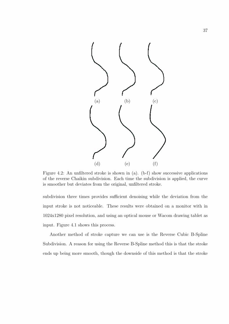
4.2 An unfiltered stroke is shown in (a). (b-f) show successive applicationsof the reverse Chaikin subdivision. Each time the subdivision is ap-plied, the curve is smoother but deviates from the original, unfilteredstroke. . . . . . . . . . . . . . . . . . . . . . . . . . . . . . . . . . . . 37

5.1 (a): A tube surface created with one stroke. (b): a rotational blend-ing surface created with two strokes. (c): A cross sectional blendingsurface created with three strokes. (d): a B-Spline patch created withfour strokes. . . . . . . . . . . . . . . . . . . . . . . . . . . . . . . . . 41

5.2 Here are some models created with our sketch system, and parts ofeach model were created using tube surfaces. The flower uses a tubesurface for the stem, and the demon’s arms and pitchfork were alsocreated using tube surfaces. Shown below the models are the strokesused to create them. . . . . . . . . . . . . . . . . . . . . . . . . . . . 42

5.3 Construction of a tube surface. Left: S(u) is the input stroke. Acircular cross section, Cu(v) is pictured in red. It lies in a plane whosenormal is tangent to S(u) at u, and is centered at S(u). This tangentvector is shown in purple. For each u, we use give the associated circlea constant radius. The resulting tube surface is shown on the right. . 43

5.4 A rotational blending surface. The left and middle images show theconstructive curves (green), ql(u) and qr(u), the center curve c(u)(blue), and a circular slice of the surface, denoted tu(v). The rightimage shows a completed surface overlaid with the blending curvesformed by holding v constant. . . . . . . . . . . . . . . . . . . . . . . 45

x

5.5 A variety of shapes is possible to generate using few strokes (top row)by using just rotational blending surfaces. We created the pear in fourstrokes, the candle in eight and the laser gun in six strokes. . . . . . . 46

5.6 A unit circle from the cylinder has been mapped via an affine trans-formation to the pear. All rotational blending circles can be thoughtof as a cylinder where each circle in the cylinder has undergone atransformation. . . . . . . . . . . . . . . . . . . . . . . . . . . . . . . 48

5.7 From left to right: sketching two constructive strokes (black), onecross sectional stroke (red) and the resulting leaf model in front andside views. . . . . . . . . . . . . . . . . . . . . . . . . . . . . . . . . . 50

5.8 Modeling a sword blade using cross sectional blending surfaces. Toprow, left to right: drawing the constructive curves only (dotted lines)results in a perfectly rounded object. Sketching the cross sectionaloutline (red line) results in a better, sharper, faceted blade. Bottomrow: the sword in a different view. Notice the final surfaces, withsharper features . . . . . . . . . . . . . . . . . . . . . . . . . . . . . . 51

5.9 A sphere being projected onto a 2D plane. The dotted line shows howthe 3D shape is being projected onto a 2D plane. Notice that thedotted line passes through two points on the sphere, one on the backof the sphere, and one in front. This means that two points on thesphere are projected to the same point on the 2D plane. . . . . . . . . 53

5.10 The user hovers the mouse cursor near where he wishes to create across section. A sample cross section, indicated by the dashed andsolid grey lines appears. This sample cross section is the similar tothe cross section of a cylinder, and is inspired by the style of Figure5.12. The dashed grey line indicates a concave cross section, while thesolid grey line indicates a convex cross section. The user can drawon any kind of cross section, even one that is sometimes convex andsometimes concave. The dashed blue line indicates a perfectly straitcross section, one that cannot be considered concave or convex. Figure5.11 shows some sample cross sections using this interface. . . . . . . 55

5.11 Concave and convex cross sections. The cross sections (grey) in (a-c)were drawn using the interface pictured in Figure 5.10. (d-f) are theresulting surfaces. (a) shows a convex cross section and (d) shows theresulting surface. (b) shows a similar, though concave cross sectionand (e) shows the resulting surface. (c) shows a cross section thatwhich is both concave and convex, and (f) shows the resulting surface. 56

xi

5.12 A diagram picturing a cylinder. The dashed lines indicate a hiddensurface. Hidden surfaces would normally be hidden from our view,but portraying them can be useful in some cases. Portraying hiddensurfaces in the same way as their non-hidden counterparts can causeconfusion. Besides using dashed lines, other colors or line styles can beused to portray a hidden line. We based our solution to the problemof convexity upon this kind of hidden line rendering, in our system adashed line indicates a concave surface (going into the paper, or behindthe basic cylinder) while a solid line indicates the convex surface. . . 57

5.13 Four categories of input strokes and resulting surfaces in our sketch-based modeling approach. (a): Two construction curves (black) andthree cross sections (blue). (b): The resulting surface, if we do not usea B-Spline to blend in between cross sections, and instead use eachcross section as a row of points in a basic mesh. (c): The resultingsurface if we interpret each cross section as a row of control points ina B-Spline. Notice that (c) has a smooth join between cross sections. 58

5.14 Left: A spaceship. The white portion of the ship was modeled usingthree cross sections, which have been smoothly blended because ofthe B-Spline method. Right: Garlic that has been modeled using twocross sections. The top of the garlic is round and requires a semi-circular cross section, while the middle and bottom of the garlic isbumpy and requires a bumpy cross section. . . . . . . . . . . . . . . . 59

5.15 (a): Two construction curves (black) and three cross sections (grey).(b): The resulting B-Spline patch created by using each cross sectionas a row of control points. Notice how this patch does not respect theconstruction curves. (c): Here we have used linear interpolation tocreate more cross sections. Notice how the patch pictured in (c) doesrespect the construction curves. . . . . . . . . . . . . . . . . . . . . . 60

5.16 (a): A control mesh for a B-Spline patch. (b): A B-Spline patchcreated from subdividing the control mesh once in the u direction.(c): The patch after one subdivision in the v direction. (d): Thepatch after two subdivisions in the u and v directions. (e) A gouraudshaded version of the patch shown in (d). . . . . . . . . . . . . . . . . 62

xii

6.1 The orthogonal deformation stroke in action. (a) the surface wewish to deform; (b) its constructive curves ql(u), qr(u), the centercurve c(u), and a cross section of the surface tu(v); (c) the surface asviewed from the side, notice that ql(u), qr(u) and c(u) are all the same,straight line when viewed from this angle; (d) the deformation stroked(u); (e) the cross section and the strokes morphing to the deforma-tion stroke (the camera angle has been slightly altered for clarity); (f)the final, deformed surface. . . . . . . . . . . . . . . . . . . . . . . . . 64

6.2 Left: perspective view of three deformation strokes (in white) appliedto the single leaf model of Figure 5.7. Right: artistic composition usingour system illustrating the shape and color progression of autumnleaf. The stem was modeled as a rotational blending surface. Theleaf of Figure 5.7 is placed at the top of the stem. The other threeleaves are deformations of this top leaf using three different orthogonaldeformation strokes. . . . . . . . . . . . . . . . . . . . . . . . . . . . 67

6.3 A skirt modeled with cross sectional oversketch. Top row, left toright: starting with a simple tube, the user selects a cross section ofthe surface. Next, the user redraws a section of it and this edits thesurface. Bottom row: the surface is rotated and drawn upon further,and the results are shown with both toon and Gouraud shading forclarity. . . . . . . . . . . . . . . . . . . . . . . . . . . . . . . . . . . . 68

6.4 Modeling a dagger handle from an existing drawing. From left toright: starting with the existing drawing Gunner’s Dagger (Copyright1998-2004 Rio Aucena. Used with permission), the user sketches 11strokes to model five specific parts of the original drawing. The bladeis modeled as a cross sectional blending surface (3 strokes) and theother four parts are modeled as rotational blending surfaces (2 strokesper surface). The final model is then rendered with both Gouraud andnon-photorealistic shading. . . . . . . . . . . . . . . . . . . . . . . . . 69

7.1 (A): Cel (AKA toon) shaded art from an animated cartoon, Bug inMouth Disease (Copyright Homestar Runner). (B): Cel shaded artpromoting the animated series, Cowboy Bebop (Copyright ColumbiaTriStar). Our toon shader is based on the type of cel shading shownin (A) and (B). (C): Line art, from [Loo43]. (D): Ink, wash, and chalkdrawing by the Renaissance master Cambiaso [Hal83]. Our HBEDrenderer is based on the types of art shown in (C) and (D). . . . . . 71

xiii

7.2 Comparison between two shading models, (a) Gouraud, (b) toon. Al-though the two shading models are mathematically similar, the toonshaded models are aesthetically different. Cartoons do not seem im-posing and add to the feeling of accessibility. Also, the hand drawnnature of sketch based modeling seems to fit better with toon shading. 72

7.3 (a): A plot of Equation 7.1 over the entire [0, 1] domain. (b): Athresholded version of Equation 7.1. . . . . . . . . . . . . . . . . . . . 74

7.4 Diffuse thresholding. (a): The left column of the table shows the valueof the dot product between the normal vector and the light vector.The right column of the table shows what each range of dot productsis thresholded to. (b): Two ramps, the top ramp shows diffuse colorvalues without thresholding and the bottom shows diffuse color valueswith thresholding. (c): Teapot without thresholding applied. (d):Teapot with thresholding applied. . . . . . . . . . . . . . . . . . . . . 76

7.5 Specular thresholding. (a): The left column of the table shows thevalue of the dot product between the normal vector and the lightvector. The right column of the table shows what each range of dotproducts is thresholded to. (b): Two ramps, the top ramp shows spec-ular color values without thresholding and the bottom shows specularcolor values with thresholding. (c): Teapot without thresholding ap-plied. (d): Teapot with thresholding applied. . . . . . . . . . . . . . . 77

7.6 The handle of a dagger. (A): The handle as drawn by an artist. (B):The handle as rendered with HBED. Notice the similarity to (A). . . 78

7.7 Here we see two different renderings of the same seashell. The imageon the left has been gouraud shaded, while the one on the right hasbeen rendered in HBED. The right image is definitely easier to makeout. . . . . . . . . . . . . . . . . . . . . . . . . . . . . . . . . . . . . 78

7.8 (a): A triceratops that has been rendered using standard Phong light-ing. (b-c): Temporary buffers of HBED, along with a final result (d).In (b), the surface normal has been rendered into the RGB channel.In (c), we see that the depth value (distance from the viewer) has beenrendered into the alpha channel. Darker values denote closer distances. 80

7.9 (a): A stylized pear rendered using a modified HBED system. HBEDhas been modified to also include some toon shading to simulate anink wash. The image was composited onto a picture of a piece of handmade, slightly colored paper. Kernel D in Figure 7.10 was used. (b):A pear rendered using Kernel C in Figure 7.10 HBED approach. (c):For contrast, we show a phong shaded pear here. . . . . . . . . . . . . 83

xiv

7.10 The image processing kernels used in HBED. Each number representsa pixel’s weight. Kernel A is used when rendering lines in a stylesimilar to that in Figure 7.7. Kernel B is used when rendering linesin a style similar to that in Figure 7.6. Since Kernels A and B havefour nonzero values in them, the each require four lookups into texturememory per pixel. Kernels C and D are similar to A and B respec-tively, except C and D only require two lookups into texture memory.C and D are very good approximations to A and B, and they are muchfaster, so our implementation uses C and D. . . . . . . . . . . . . . . 83

8.1 Cartoon-like shapes. From top to bottom with total number of strokessketched by the user in parenthesis: paprika (2) and tangerine (2)(both sketched directly over the spiral method drawings in Figure 1.1),pumpkin (5), bad guy (19), Wizard (57), and snoopy (10). . . . . . . 86

8.2 Cartoon-like shapes. Vulpix, a cartoon fox took 13 strokes to make,while Oddish, a cartoon radish, took 15. . . . . . . . . . . . . . . . . 87

8.3 The construction of a spaceship, which has multiple cross sections.The final ship is in (A). The nosecone, rocket, and cockpit consistof rotational blending surfaces, but the body (B) needs multiple crosssections, and in our system this makes it a B-Spline patch. The strokesused to create this B-Spline patch are shown in (C). Black strokes arethe construction curves, while red ones are the cross sections. (D)shows the body of the ship from the same view as (C). Note that thecross sections in (C) are very different from each other. . . . . . . . 88

8.4 The construction of a fish. The final fish is in (A). We see the fish’shead in (B), this portion will require multiple cross sections, and in oursystem this makes it a B-Spline patch. The strokes used to create thisB-Spline patch are shown in (C). Black strokes are the constructioncurves, while red ones are the cross sections. (D) shows the head ofthe fish from the same view as (C). The cross sections in (C) had tobe different from each other to make the fish’s nose stick out. . . . . 89

8.5 Rose, modeled in 23 strokes. The petals and the three stems weregenerated in 2 strokes each using rotational blending surfaces. Eachleaf was generated with 3 strokes using cross sectional blending sur-faces (Figure 5.7), distorted (Section 6.2) and interactively placed atthe stem using standard rotation/translation modeling tools similarto the ones found in Maya [Aut06]. Bottom image: (left) the twostrokes sketched for the rose petals; (middle and right) real botanicalillustrations were used as templates for sketching over the leaves (twomiddle leaves [Wes83] and a sample from a painting). . . . . . . . . . 90

xv

8.6 Pyramidalis Fructu Luteo (yellow berries), modeled in 33 strokes. Theberries and the stem were generated in 2 strokes each using rotationalblending surfaces. Each leaf was generated with 3 strokes using crosssectional blending surfaces (Figure 5.7). Bottom left image: The usersketched directly over nine specific parts of a real botanical illustrationof yellow berries (Copyright 2004 Siriol Sherlock. Used with permis-sion.): one stem, three leaves and five berries (right image). In themodel, all leaves and berries are instances of these nine sketched-basedobjects. Each of the leaf instances was properly distorted (Section 6.2)and both leaves and berries were then placed at the stem by the userwith standard modeling tools. . . . . . . . . . . . . . . . . . . . . . 91

A.1 Left: A menu bar from a windows application. The menubar consistsof several pulldown menus. Right: The menubar in our system, whichis based on the windows style menubar. . . . . . . . . . . . . . . . . . 97

A.2 Above: The mode tape arrow is in the bottom corner of the screen.Below: Clicking on the arrow expands the mode tap to look like aseries of buttons. Clicking on the arrow again contracts the mode tape.102

A.3 Above: The lathe tape arrow is on the right edge of the screen. Below:Clicking on the arrow expands the lathe tap to look like a series ofbuttons. Clicking on the arrow again contracts the lathe tape. . . . . 103

A.4 A B-Spline surface created from the strokes pictured to the left. Themiddle image shows this surface without a back, while the right imageshows it with a back. The back of the surface mirrors the front of thesurface exactly. . . . . . . . . . . . . . . . . . . . . . . . . . . . . . . 103

A.5 When in selection mode, you can select a surface by clicking on it.Several new buttons come onto the lower right portion of the screenonce you have clicked on a surface. . . . . . . . . . . . . . . . . . . . 107

A.6 The rotate panel. You can rotate the object along the x, y, and z-axes.These axis are relative to the camera angle, and can be considered tobe the axes of screen space. For instance, the z-axis is pointing out ofthe screen, regardless of the camera rotation. . . . . . . . . . . . . . . 108

A.7 The translation interface. The red arrow can be clicked and draggedto move the surface around in the direction of the x-axis. The greenand blue arrows work for the y and z-axis, respectively. The yellowsquare allows you to translate around in the view plane, and is oftenmore useful than the arrows. . . . . . . . . . . . . . . . . . . . . . . . 109

xvi

A.8 The extended color dialogue. Clicking on a sphere changes your sur-face’s color properties so that the surface’s lighting resembles that ofthe sphere. This is often more convenient than changing the color viaone of the color sliders, but the color sliders can be used to createcolors that aren’t present in the extended color dialogue. . . . . . . . 110

A.9 The subdivision editor. When we create B-Spline patches, we usesubdivision. Here, we can control the number of subdivisions, as wellas the relative size of the control mesh, which is related to the samplingrate. . . . . . . . . . . . . . . . . . . . . . . . . . . . . . . . . . . . . 110

C.1 The modern graphics pipeline is broken up into these stages. This is asimplified look at the pipeline, more complicated versions are availableand these can vary per video card. . . . . . . . . . . . . . . . . . . . . 119

xvii

Chapter 1

Introduction

In traditional illustration, the depiction of 3D forms is usually achieved by a series

of drawing steps using few strokes. The artist initially draws the outline of the

subject to depict its basic masses and boundaries. This initial outline is known as

constructive curves or contours and usually results in very simple geometric forms.

Outline details and internal lines are then progressively added to suggest features

such as curvatures, wrinkles, slopes, folds, etc [DGK99, Gol99, Gup77] (shown in

Figure 1.1).

Using the spiral method, shape depiction is achieved by the use of quickly

formed spiral strokes connecting the constructive curves, creating a visual “blend”

of the overall volume between the constructive curves. Spiral strokes are helpful when

irregular rounded forms are involved, such as fruits, vegetables, or when modeling

stuffed animals because overall they are rounded and puffy.

The scribble method involves the use of continuous stroke(s) placed between

constructive curves. The scribbled strokes are typically used to depict specific folds,

bumps, etc., across the subject. In Figure 1.1, a single scribbled stroke defines the

fold pattern at the boundary end of the skirt.

The bending (or distortion) method illustrates how artists visualize adding

unique variations to an initial sketch or visual idea of the subject. These variations

aid on depicting the overall shape of subjects which naturally present a large vari-

ety of twists, turns, and growth patterns, such as botanical and anatomical parts.

1

2

Though this method is not present during the process of creating a finished drawing,

it is useful when conceptualizing or contemplating a form. We have developed a

sketch based way of deforming a 3D model that is similar to this distortion method,

though our method both visualizes the distortion and can actually perform the dis-

tortion.

Another common method used by artists to communicate visual form is the

rendering of cross sections. These cross sections allow us to get a better grasp as to

the nature of the shape being portrayed. Cross sections are generally not present

in finished drawings, but are used to communicate the general idea about a shape.

An example of cross sections from an art book can be seen in Figure 1.2 and Figure

1.3. We have found that cross sections can also be used to communicate a shape to

a computer modeling program, and aid themselves nicely to sketch based design.

Existing 3D modeling techniques can model many types of objects, but they are

not without problems. For instance, most existing computer modeling techniques

are based on control point manipulation (see Section 3.4). This includes popular

modelers such as Maya [Aut06]. Though the control point method is very popu-

lar and highly accurate, it has some drawbacks. As the number of control points

increases, the amount of control points we must manually position can increase as

well. In our system, this isn’t really as much as a problem. Although our surfaces

are actually B-Spline patches (see Section 5.5.2), the amount of work the user must

do isn’t proportional to the amount of control points in the patch. In fact, our

system avoids dragging control points completely, though it isn’t incompatible with

such an approach. Another key problem is that most surfaces are modeled by artists

using programs that aren’t based upon any type of artistic technique. An artist’s

3

Figure 1.1: Traditional hand-drawn techniques for progressive shape depiction[Gol99] [DGK99] [Gup77]. Skirt drawing, Copyright 1998-2004 Rio Aucena. Usedwith permission.

4

Figure 1.2: A figure from an art book, “Figure Drawing For All It’s Worth” by An-drew Loomis [Loo43]. This figure illustrates various shapes by using cross sections.Though these cross sections wouldn’t be present in a finished work, they are usefulwhen describing form to other artists, or in our case, to a computer.

5

Figure 1.3: A figure from an art book, “Drawing the Head and Figure” by JackHamm [Ham63]. This figure illustrates the form of the nose by using cross sections.Though these cross sections wouldn’t be present in a finished work, they are usefulwhen describing form to other artists, or in our case, to a computer.

6

well-honed ability to draw can more directly lend itself to sketch based modeling.

In this thesis we present a sketch-based modeling system inspired by the tradi-

tional illustration methods above. We have developed new algorithms to facilitate

the rapid modeling of a wide variety of free-form 3D objects, constructed and edited

from just a few freely sketched 2D line segments, without imposing any constraints

regarding the order in which lines are entered as well as their spatial relationship.

As input, our system takes strokes which are sketched by the user using a mouse

or tablet. Each stroke is then captured and properly filtered (Chapter 4). We propose

various ways of using these strokes for efficient and robust modeling of 3D objects

(Chapter 5). The modeling comes in two phases: creation and editing (Chapter 6).

The techniques we developed, at each phase, were inspired by the traditional shape

sketching methods of spiral, scribble , bending (Figure 1.1) and cross section (Fig

1.2 and 1.3).

1.1 Contributions

In contrast to previous approaches, which are discussed in Chapter 2, our system

provides the means to (1) generating a large variety of 3D parametric surface objects

with curved and creased features (see Figure 5.5 or Chapter 8). Furthermore, (2)

few strokes are required to create and edit the surfaces (shown in Chapter 5-6). Also,

by following traditional methods gleaned from pen and paper, (3) we have devised

simple interaction idioms to allow efficient and robust stroke capturing (Chapter

4). Finally, (4) our boundary and surface editing paradigm (Chapter 6) is quite

flexible to support the application of both subtle and drastic variations to instances

7

of sketched objects.

1.2 Organization of the Thesis

In Chapter 2 we discuss previous work in sketch based modeling. Chapter 3 gives

background information on parametric surfaces, which are important because our

sketch based models are also parametric. In Chapter 4 we present our method for

stroke capture and conversion to parametric form. In the creation phase (Chap-

ter 5), we use strokes to generate several new types of parametric surfaces, as well

as B-Spline patches. In the editing phase (Chapter 6), subtle or drastic variations

to the surfaces can be added by using a single deformation stroke (Section 6.1)−

approximating the bending method. Surfaces can also be modified by oversketching

cross-sections of the model (Section 6.2) − which is related the scribble method. A

complete discussion on existing sketch based methods is in Chapter 2. Results gener-

ated using our system are discussed in Chapter 8. Finally, we draw some conclusions

in Chapter 9.

Chapter 2

Sketch Based Modeling

Sketch-based interface and modeling systems are a relatively new area in modeling.

The main goals of sketch-based systems include allowing the creation of 3D models

by using strokes which are extracted from user input and/or existing drawing scans.

Another goal of sketch modeling is to make modeling more intuitive and/or rapid,

specifically by having a better user interface with which to interact, or by allowing

modeling to be performed with no interface at all. Sketch-based systems can be

classified in two groups [NJC+02]: Geometric Reconstruction and Gestural Modeling.

Using the Geometric Reconstruction approach [NJC+02] [VSMM00], a 2D image

is provided by the user. The system then tries to reconstruct a 3D model from this

2D image. Note the similarity of this approach to the general problem of computer

vision.

Gestural Modeling includes systems that allow the user to construct and edit 3D

objects by taking various hand gestures as input. These systems tend to interpret

data input from a mouse or drawing tablet as gestures. Different gestures signify

different modeling operations to the system. For example, drawing a wavy line

quickly may indicate that the user wants to erase a portion of the model. Ultimately,

spatial and/or temporal information about the input data as well as the previous

actions of the user determine the reaction of the system. Our system falls into this

category, and so we will next review some of the previous work that has been done

on gestural modeling.

8

9

2.1 Gestural Modeling

In this section we will review selected papers within the category of Gestural Mod-

eling.

SKETCH [ZHH96] uses mouse gestures to create and modify 3D models. To this

end, SKETCH uses gestures to create simple extrusion-like primitives in orthogonal

view. It is also possible to specify CSG operations and defining quasi- free-form

shapes such as ducts in a limited manner. In contrast with our system, SKETCH

does not allow the user to model freeform surfaces.

Quick-Sketch [EHBE97] is based on parametric surfaces. Their system creates

extrusion primitives from sketched curves, which are segmented into line and circle

primitives with the help of constraints. Other free-form shapes which can be created

with Quick-Sketch include surfaces of revolution and ruled surfaces. In all cases,

a combination of line segments, arcs and B-Spline curves were used for strokes.

Although this system can be used for sketching engineering parts and some simple

free-form objects, it is hard to sketch more complicated free-form objects such as in

Figure 1.1. Our system also introduces new types of parametric surfaces which are

specially designed for sketch modeling.

Teddy [IMT99] allows the user to easily create free-form 3D models. The system

allows creating a surface, by inflating regions defined by closed strokes. Strokes are

inflated, using a chordal axis transform, so that portions of the mesh are elevated

based on their distance from the stroke’s chordal axis. Teddy also allows users to

create extrusions, pockets and cuts to edit the models in quite flexible ways. Teddy’s

main limitation lies in that it is not possible to introduce sharp features or creases

10

directly on the models except through cuts. Furthermore, the system only allows

editing a single object at a time. Later improvements were made to Teddy. Smooth

Teddy [IH03] introduced a much needed remeshing stage, and finally Chameleon

[IC01] allowed a user to paint onto the models made by Teddy. Figure 2.1 shows

some results from Chameleon.

Teddy was the main inspiration for our work, but there are many key differences

between Teddy and our system. Although the remeshing introduced with Smooth

Teddy was an improvement, even Smooth Teddy’s mesh consists of irregularly sized

and arranged polygons, while our methods result in a regular polygon mesh (see

Section 3.2.5). The surfaces created by Teddy do not follow the user’s strokes very

tightly, and this has been another one of our goals. Another major difference from

our work is that Teddy’s surfaces are not parametric, mostly Teddy deals directly

with mesh-based operations. It is impossible to model objects with sharp corners in

Teddy without using CSG, however Teddy has CSG operations which are very well

suited for a sketch based interface, and our work lacks such operations.

Owada et al. [2003] propose a sketch-based interface similar to Teddy, which is

used to model 3D solid objects and their internal structures. Sketch-based opera-

tions similar to those in Teddy are used to define volume data. The authors present

methods for performing volume editing operations including extrude and sweep. Ex-

truding connects a volumetric surface to a new branch, or can punch holes through

the surface. Sweep allows creating a second surface on top of the original. This is

accomplished by drawing the cross section of where the two surfaces are to meet,

and a sweep path to define the place of the second surface. Using an ingenious com-

mand to hide portions of the surface, the system makes it possible to “see inside”

11

Figure 2.1: Examples from Igarashi’s Chameleon system, which allows the user tosketch shapes, perform CSG operations on them, and then paint color onto them.

the surface. By hiding portions of a model, and then using extrusions, the user can

specify hollow regions inside an object. However, this system is also not suitable

for editing sharp features or creases. Figure 2.2 shows some example models created

with Owada et al’s system. Our work is focused on parametric and not volume-based

surfaces. In our system it is impossible to edit the internal structure of objects.

Figure 2.2: Examples from Owada et al’s system. Sketch based operations are usedto define volume data and perform CSG operations on them.

Another sketching system was proposed by Karpenko et al. [KHR02]. It used

variational implicit surfaces [TO99] for modeling blobs. They organized the scene in

12

a tree hierarchy thus allowing users to edit more than one object at a time. Another

interesting feature is using guidance strokes for merging shapes. Like Teddy, this

system is not clearly suited to editing sharp features or creases into objects. A

major contrast from our work is that we are using parametric and not implicit

representations.

BlobMaker [dAJ03] also uses variational implicit surfaces as a geometrical rep-

resentation for free-form shapes. Shapes are created and manipulated using sketches

in a perspective or parallel view. The main operations are inflate, which creates 3D

forms from a 2D stroke, merge, which creates a 3D shape from two implicit surface

primitives, and oversketch, which allows redefining shapes by using a single stroke

to change their boundaries or to modify a surface by an implicit extrusion. This sys-

tem improves on Karpenko’s and Igarashi’s by performing inflation independently of

screen coordinates and a better approach to merging blobs. Figure 2.3 shows some

results of the BlobMaker system, as well as its minimalized interface.

Like other systems previously reviewed, BlobMaker does not provide tools to

create sharp features. Another major difference from our system is that we are

dealing with parametric surfaces and BlobMaker is concerned with implicit surfaces.

Varley et al [VSMM00] give a method that generates a 3D mesh based upon

user-input strokes. Their method assumes that the output mesh is geometrically

similar to a pre-defined template. The camera position and orientation are esti-

mated based upon the spatial layout of the strokes and the template. The authors

discuss various methods of extracting and reconstructing meshes using the camera

and stroke information. They again use the template to determine where each of

these reconstruction methods is applicable. The mesh is ultimately constructed as

13

Figure 2.3: Examples from Araujo et al’s BlobMaker system. Also pictured is itsminimalized interface. The Blobmaker system allows the user to sketch and editvariational implicit surfaces interactively.

a collection of Coon’s patches. In the same paper they also propose a method of B-

Rep reconstruction using similar stroke data. The B-Rep reconstruction method has

several phases, including preprocessing, geometric reconstruction step which tries to

generate geometry based upon various constraints (interpretations of how the user’s

drawing should correspond to 3D geometry) extracted from the user’s drawing, some

of which may be at odds with one another, and a “finishing” phase, which attempts

to satisfy as many of the constraints as possible. Varley et al. also present a novel

stroke capturing algorithm which they use in both their B-Rep and 3D mesh meth-

ods. This algorithm allows the user to draw strokes in a style similar to the one many

artists and engineers use when they sketch on paper. In this style, many shorter sub-

strokes are used to compose each stroke. They refer to the group of sub-strokes as a

“bundle of strokes.” Their algorithm interprets each “bundle of strokes” as a single

stroke. In their method, only intersecting strokes are considered to be part of the

14

same bundle. Our system does not follow a template-based approach. Our goal was

to allow the user to freely sketch any type of model represented as paramteric sur-

faces not following any particular constraints from pre-defined templates. In contrast

to the the bundle of strokes method, our system processes long, continuous strokes.

Duncan and Swain [2004] propose the SketchPose system, which allows designers

to quickly sketch control points using a pen. They have derived novel techniques

drawn from conventional pencil-and-paper cartooning methods. Moreover, their

technique also stresses sketching on the view plane. This greatly simplifies posi-

tioning and deforming objects, thus expediting the definition of poses for animated

characters. Sketchpose is mainly concerned with positioning the various parts of ex-

isting 3D models, while our system is more concerned with creating new 3D models.

Ijiri et al. [IOOI05] present a sketch-based system for specialized generation and

editing of plants, including leaves, stamens, petals, sepals, and other plant organs.

A leaf is modeled after the user skecthes its outline, which is then parameterized and

turned into a set of control points for a B-Spline surface. When editing the leaf, the

user can draw on a modifying stroke, which is similar to the deformation stroke in

Section 6.1. The modifying stroke helps the user to edit the overall shape of the leaf

by moving any of the leaf’s control points with a single stroke, as opposed to clicking

and dragging each one. Their system also provides a user interface that can create

some of the branching structures found in plants. However, their system is targeted

to modeling floral features such as leaves or petals, whereas our system allows the

modeling of general types of objects.

There are several commercial packages which use sketching for geometric model-

ing. SketchUp [2005] is a package with a very well thought-out interface that allows

15

architects to quickly sketch and directly manipulate 3D drawings of buildings using

plane faces and extrusion. Unlike our system, SketchUp has no support for curved

surfaces. The models that a user can create with SketchUp are limited to buildings

and houses, whereas our system is designed for more general purposes. VRMesh

[2005] is able to create triangular meshes from sketches using an inflation approach

similar to Teddy, but it mostly focuses on importing point cloud data (vertices with-

out face information) and editing this data via sketching and other means, but it

generally doesn’t deal with parametric surfaces. Curvy 3D [2005] models surfaces us-

ing 2D sketches. It also allows the user to paint height maps (used in bump mapping)

and color maps onto the model.

2.2 Theoretical Limits of Sketch Based Modeling

In general, the overall goal of sketch based modeling is to allow the user to create

a 3D model mainly by drawing on the computer screen. This main goal yields four

sub-goals as well in which the system must: (1) require little training, (2) allow the

user to create models rapidly, (3) provide an environment that the user is, overall,

pleased with, and (4) foster the user’s creativity.

Concerning item (1), it is probably possible to create a system that requires no

training for the user. Such a system would only be limited by the user’s ability

to draw. An even stronger system would create beautiful models even if the user’s

drawing skills were limited or non-existent. Both gestural modeling and geometric

reconstruction can probably one day meet this kind of goal, though the inherent

ambiguity of taking a 2D image data and transforming it into a 3D model might

16

limit geometric reconstruction in some 3D models.

Moving on to item (2), theoretically, gestural modeling could create a 3D model

faster than the user could sketch it on paper. For instance, it might take a user twelve

strokes to depict a house on paper in 2D, while it might take the user less strokes

to depict it in 3D on a computer modeling program. This might be especially pos-

sible when using a program dedicated to modeling houses. Another favorable point

is shading. Computer programs can shade automatically, using standard lighting

programs based on the surface normal and light positions, while drawings must be

shaded manually, using hatching for instance. Shading is another reason why a

computer program can theoretically create something more quickly than a user can

sketch it. On the other hand, advanced shaders must be authored. The geometric

reconstruction method might not be suitable for creating a model faster than the

user can sketch it, because it requires a sketch in the first place. Perhaps limiting

the complexity of the required sketch in comparison to traditional sketches would

speed this up, however.

Having the user be pleased with the system (point (3)) is a more subjective goal,

but users tend to be pleased with systems that they feel they are in control with,

that are responsive, and that they feel do not limit them when compared to other

systems they may have used. This means that the program must be made to act in

a consistent fashion and not lead the user by the hand, rather it must allow the user

to control every step of the process. Responsiveness can be gained by developing

and using efficient algorithms, while the goal of not limiting the user in comparison

to other systems can be achieved by making a new system as a sort of plug in. For

instance, a sketch system that was devised as a Maya plugin could take advantage

17

of all of Maya’s features. Both gestural modeling and reconstructive geometry could

produce systems that were favored by users.

Concerning a creative environment (point (4)), a blank sheet of paper is the

ultimate creative environment, upon which all manner of media and styles can be

applied, and perhaps sketch based modeling can inherit some of this because it

generally resembles sketching on paper, though I find it hard to imagine any system

with the flexibility of a simple piece of paper and pencil. Though pencil and paper do

not carry with it some of the advantages of 3D modeling, such as ease of animation,

it certainly remains versatile. Reconstructive geometry probably has the edge in this

case.

It is difficult to claim our system has met point (1) without extensive user studies

comparing the learning curve of our system to other popular systems. Since there

aren’t many necessary operations to learn to use our system, one would expect it to

be easy to learn to use. On the other hand, if the user is particularly bad at drawing,

our system may not be very easy to learn (in general, those with poor motor skills

will find it hard to model using ANY platform). This is somewhat offset by the fact

that most 3D modeling is done by artists and most artists can, at the very least,

draw.

Our system goes a makes progress towards point (2). Most of the models we

created using our system can be made in a few minutes. The slowest part of our

system, the assembly of parts, isn’t sketch based at all but rather relies upon clicking

and dragging in a fashion exactly the same as Maya’s translation interface [Aut06].

Drawing the actual parts is extremely fast, and is only limited by the speed in which

the user can draw.

18

Point (3) is also difficult to prove. One thing to remember when thinking of

this point is that our system is efficient enough to run in realtime. This kind of

responsive behavior goes a long way towards making users happy. Another strength

of our system is that follows the user’s strokes exactly, which gives a good sense of

control. A third good point is that many artists enjoy drawing and even draw in

their free time. A system that allows them to draw would be favorable.

Concerning Point (4), in a way, our drawing system simulates a piece of paper.

There is nothing with more room for creation than a blank sheet. The sketching

operations also lend themselves to a sort of creative behavior, as they are very quick

and can be used for experimentation without taking much time up.

Chapter 3

Parametric Surfaces

In computer graphics, parametric surfaces are probably the most common type of

surface. Since our system uses new kinds of parametric surfaces, here we give a

general discussion on parametric surfaces and their benefits. We also give some

examples of popular parametric surfaces that are related to our methods.

3.1 Definition of a Parametric Surface

Parametric equations express quantities as functions of independent variables called

parameters. One well-known parametric equation is the parametric form of a unit

circle (a circle with a radius of one):

Q(t) = (x(t), y(t))

x(t) = cos(t)

y(t) = sin(t)

R is the radius of the circle, and t is allowed to range from zero to 2π. You

can write this as t ∈ [0, 2π], and [0, 2π] is called the parameter domain. Parametric

functions are only considered to be defined over the paramter domain.

This kind of definition easily extends to 3D. For example, we can create a cylinder

instead of a circle. A cylinder can be thought of as a circle moving up along a straight

line. The parametric definition is:

19

20

Q(s, t) = (x(t), y(t), z(s))

x(t) = r cos(t)

y(t) = r sin(t)

z(s, t) = s

Here again t ∈ [0, 2π], and s ∈ [0, L], where L is the length of the cylinder.

Because Q(s, t) takes in two parameters, we can say that it has a 2D parameter

space, or a 2D domain. Also, since Q(s, t) is a 3D shape and not a curve, we can say

that it is a parametric surface. Using other parametric equations, we can create a

variety of parametric surfaces and curves which are used in computer graphics, some

of which are shown in Sections 3.3 through 3.4.

3.2 Benefits of Parametric Surfaces

Although there are many different kinds of parametric surfaces, they all carry some

common benefits.

3.2.1 Texture Coordinates

Texture maps remain a popular technique for increasing detail in 3D modeling. Tex-

ture maps can contain color information, information about the surface normal for

use in bump maps, or any other information useful to rendering. Parametric sur-

faces with two parameters (a 2D domain) lend themselves immediately to texture

mapping, as the texture coordinates can usually be a function of the same two pa-

21

rameters that define the surface. Even better, this function is usually just a very

simple affine transformation.

Take, for example, the parametric equations that describe a torus.

Q(u, v) = (x(u, v), y(u, v), z(u, v))

x(u, v) = (a + b cos(v)) cos(u)

y(u, v) = (a + b cos(v)) sin(u)

z(u, v) = b sin(v)

Here, a is the inner radius of the torus and b is the outer radius of the torus. The

parameters u and v range from zero to 2π. We can use texture coordinates where:

tx =u

2π

ty =v

2π

where tx and ty are the texture coordinates in the x and y directions. The u

and v coordinates are being divided by 2π because texture coordinates are typically

required to be in the range [0, 1]. Figure 3.1 shows a torus texture mapped in this

way.

3.2.2 Varying Level of Detail

In some situations, we wish to conserve the number of polygons. For instance, in

creating a realtime application we must realize that only a certain number of triangles

22

Figure 3.1: Top Left: A 2D texture. The rest of the figure shows a torus from variousangles. It has been texture mapped according to Equation 3.1.

can be rasterized and lit, texture mapped, etc, per second while keeping high frame-

rates. In other situations, we might want to use the highest quality models we can

find. High quality models work best in situations where we are pre-rendering. Movies

can use pre-rendering, as we can render each frame to a series of image files and then

play all the image files one after the other while viewing the movie. Another situation

that calls for high quality models is when we take screenshots for printing in a book

or other manuscript.

Parametric surfaces can have varying levels of detail. That is, they can work well

when you need a high polygon count or a low count. This property stems from the

fact that we can sample the domain of the parametric function as many times as we

wish, and use each of these samples as parameters to the parametric function. The

higher the sampling rate, the more accurate the surface is. Lower sampling rates, on

the other hand, reduce the number of polygons. Figure 3.2 uses the torus example

to illustrate this point.

23

(A) (B)

(C) (D)

Figure 3.2: A: A torus with only four samples in the u and v directions. B: A toruswith eight samples in the u and v directions. C: A torus with 16 samples in the uand v directions. D: A torus with a high number of samples, 210 in both the u andv directions.

24

3.2.3 Stripped Geometry

Strip geometry generally means having a sequence of triangles or quads share edges

in a strip like pattern. A series of triangles which all share vertices resembles a strip

of triangles, see Figure 3.3. A quad strip is similar to a triangle strip, except that we

have a series of adjacent quads instead of triangles. Because of graphics hardware

reasons, rendering a strip of n polygons is faster than rendering the same n polygons

separately. Another benefit of stripping geometry is that less data needs to be stored

and transfered. Sharing vertices can lead to a more efficient data structure because

there are less redundant vertices. Furthermore, on modern graphics cards stripped

geometry renders much faster than non-stripped geometry (about 66% faster), and

this is of key interest because we wish to retain high frame-rates.

Figure 3.3: A strip of four triangles. Notice that there only six vertices in all if thetriangles can share vertices, but there are twelve vertices if the triangles can’t sharethe vertices. In a triangle strip, the first triangle needs to specify three vertices,and all other triangles need just one vertex each. Quad strips are similar to trianglestrips.

3.2.4 Reduced Storage and Transmission

Although a parametric surface can be evaluated to have thousands of polygons, we

need not store all of these. Rather, we can just store certain model attributes. For

25

instance, in a torus you would need to store the radian a and b, and perhaps the

number of evaluations you want in the u and v directions. Compare this to storing

every single polygon in the torus, which may number in the thousands depending

on the sampling rate of u and v. This argument extends to transmission of data as

well.

3.2.5 Regular Polygon Mesh

The tessellation in parametric surfaces tends to have a regular pattern. This is

beneficial for several reasons. When lighting is applied to the surface it tends to

behave in a more uniform fashion. It is also generally easier to store such a surface

because we know the number of vertices in each polygon in advance (for instance, if

every polygon is a quad). Additionally, algorithms that need to behave differently

based on valence or the geometry of neighborhoods of polygons will require less

separate cases on regular geometry. In some cases, it is even possible to store such

a polygon mesh as a texture.

3.3 Common Surfaces

The so-called common surfaces occur frequently in mathematics and in computer

modeling. They have simple and efficient parametric descriptions, but they are not

sufficient for modeling many types of objects. In our system we have introduced new

types of surfaces which are similar to the common surfaces (and these are discussed

in Chapter 5). In this section we will review some of the common surfaces.

26

3.3.1 Surface of Revolution

By rotating a 2D curve about an axis, we generate a surface of revolution. Figure

3.4 gives some examples of surfaces of revolution and their respective curves. Given

a 2D curve c(t) = (x(t), y(t)), the parametric description of a surface of revolution

about the y-axis is

Q(s, t) = (Qx(s, t), Qy(s, t), Qz(s, t))

Qx(s, t) = x(t)cos(s)

Qy(s, t) = y(t)

Qz(s, t) = x(t)sin(s)

where s is allowed to range from zero to 2π, and it may be helpful to imagine

each point on the curve c(t) being swept out along a circular path about the y-axis.

(A) (B) (C) (D)

(E) (F)

Figure 3.4: Surfaces of revolution and their generating curves.

27

3.3.2 Ruled Surface

Another useful type of surface is the ruled surface. A ruled surface requires that we

have any two curves with the same parameterizations a(t) and b(t). For each t, we

can draw a line segment from a(t) to b(t), and we have our ruled surface.

Q(s, t) = (1− s) ∗ a(t) + s ∗ b(t) (3.1)

where s ranges from zero to one, and t keeps its original range as a parameter

of a(t) and b(t). Figure 3.5 shows some examples of ruled surfaces. It is probably

possible to connect a(t) and b(t) by a curve instead of a straight line, but I haven’t

heard of this being done before. Another extension could be higher dimensional ruled

surfaces. For example, the next dimension of ruled surface would have A(u, v) and

B(u, v) represent regular ruled surfaces, and we have a ruled surface C(s, u, v) which

connects A(u, v) and B(u, v) at all u and v. This could also be considered a ruled

volume. I’m not sure if higher dimensional ruled surfaces would be very useful.

3.3.3 Generalized Cylinder

A generalized cylinder is a particular class of ruled surface. Whereas a ruled surface

requires two curves a(t) and b(t), a generalized cylinder requires only one curve c(t)

and a direction vector ~d. The curve starts at the origin, and moves in the direction

specified by ~d. Equation 3.2 represents a generalized cylinder over c(t):

C(s, t) = s~d + c(t) (3.2)

where C(s, t) is our generalized cylinder and s ∈ [0, 1]. The parameter range of

28

(A) (B) (C)

(D) (E) (F)

(G) (H)

Figure 3.5: Various ruled surfaces and their generating curves. (A): Two circles candefine a cylinder, shown in (B) and (C). (D): Two circles, one of radius zero, candefine a cone, shown in (E) and (F). (G) and (H): Here we see another ruled surface,the hyperbolic paraboloid. The generating curves, which are just two straight lines,are shown in red and blue.

29

t is unchanged, it just depends upon the original definition of c(t). All generalized

cylinders can be written as ruled surfaces, though the reverse isn’t true.

3.3.4 Coon’s Patch

Whereas a ruled surface requires two curves a(t) and b(t), a Coon’s patch requires

two additional curves c(s) and d(s). Additionally, there is a condition that these four

curves join at the ends. These four curves can be called edge curves. Each point on

the Coon’s patch is an affine combination of points from each of these four curves.

This can be written as:

C(s,t) = (c(t)(1-s)+d(t)s)+(a(s)(1-t)+b(s)t) -

((1-s)(1-t)c(0)+s(1-t)d(0)+c(1)t(1-s)+d(1)st)(3.3)

Here, C(s, t) represents the Coon’s patch. Figure 3.6 shows a sample Coon’s

patch that was created according to Equation 3.3.

3.4 B-Spline Patches

When a more powerful modeling method is needed, B-Spline patches can be used. In

Section 3.3.4, we described how a Coon’s patch is defined by using four edge curves.

The shape of the edge curves determines the shape of the Coon’s patch. A B-Spline

patch, similarly, is defined by using a net of control points. The positioning of the

points that make up the net determines the shape of the B-Spline patch, as shown

in Figure 3.7. Another example of a control mesh is shown in Figure 3.8.

There are several advantages to having a control net over having four boundary

curves. First, making new boundary curves requires us to enter in a new function,

30

(A) (B) (C) (D)

(E)

Figure 3.6: (A-D): Here we see the four edge curves of the Coon’s patch. (E): ACoon’s patch created by using the curves pictured in (A-D).

Figure 3.7: (Left: A control mesh (red) and the resulting B-Spline patch (blue).Right: A shaded version of the same patch.

31

Figure 3.8: A seashell and the control mesh used to create it. The seashell is a singleB-Spline patch

while positioning the control net only requires that the user click and drag the

control points (though this may become tedious if the user needs to click and drag

a great many control points). Second, in a Coon’s patch it is difficult to control

the behavior of the patch towards the center of the patch, when the surface doesn’t

really get heavily influenced by any of the user-defined boundary curves. But with

B-Splines, we can easily control the center of the patch by adjusting the control net

points which are near to the center of the patch. Finally, to a degree each boundary

curve affects the whole patch. What if we just want to influence a piece of the patch?

B-Splines have a property called local control. Local control means that each control

point in the control net only affects a local area of the patch, rather than affecting

the patch globally.

The classic method to generate a B-Spline patch is by the following:

32

Q(u, v) =M∑i=0

L∑k=0

Pi,kNi,m(u)Nk,n(v) (3.4)

Here, the control mesh is an M×L grid. The function N is the so-called B-Spline

Basis Function. This basis function is of the form

Nk,m(t) =

(t− tk

tk+m−1 − tk

)Nk,m−1(t) +

(tk+m − t

tk+m − tk+1

)Nk+1,m−1(t) (3.5)

Here, t has two meanings. First, it is just the parameter of the function N ,

and in this sense t is just a scalar value. When t is written with a subscript, for

instance tk, t represents a vector of scalar values called the knot vector. Different

knot vectors cause the B-Spline patch to behave in different ways, but there is a

standard knot vector that is used in most applications. Equation 3.4 is recursive

and is very computationally expensive. There is also an iterative method to evaluate

B-Spline patches, and this is slightly faster. But the fastest method of evaluating a

B-Spline is by using subdivision.

Subdivision is an iterative algorithm. By running the subdivision algorithm mul-

tiple times on the so called coarse control mesh, we can get a nice, smooth B-Spline

patch. The patch that results from applying subdivision is the same as the patch

that results from directly evaluating the basis function. Since subdivision can be

applied iteratively, a patch created using subdivision can be thought of as a sort

of parametric surface where the parameter is the number of iterations. Of course,

subdivision is not parametric in the same way as most of the surfaces in this chapter

are. Our system uses the subdivision method because it is faster, and it is covered

33

in Section 5.5.2.

Chapter 4

Stroke Capture

Stroke capture is the process of recording, and in some cases parameterizing strokes

from an input device such as a pen or mouse. These raw input strokes are the

elementary data type for modeling using a sketch-based approach. Therefore, every

sketch-based modeling system should offer a robust stroke capturing approach. In

contrast, other forms of modeling use points, polygons or density values (as found

in volume data) as the defining units.

Our approach is to represent the input strokes in parametric form in order to lead

to a consistent modeling of parametric surfaces. Parametric surfaces are desirable

for many reasons, and this is discussed in Chapter 3.

In our system, sketched strokes start as raw data from the mouse or pen (Fig-

ure 4.1, left). This data is an ordered set of points, and can be interpreted as a

parametric curve c(u) as follows: Given n points and restricting u to take on integer

values ranging from 1 to n, c(i) is simply the ith point.

Interpreting the raw data as a parametric curve causes three problems. First, the

points are very noisy due to the shaky nature of handling the input devices. Second,

the points are irregularly distributed along the drawing path due to variations in

drawing speed. Third, there will be a very large number of points because the input

device sends data many times per second.

Classical approaches to stroke capturing filter the noise and parameterize the

stroke in separate steps. The first pass applies point reduction and dehooking while

34

35

the second step uses line segment approximation [DP73] [PK04]. We chose to use a

more simple method of stroke capture that yields a smooth and compact approxi-

mation to the input stroke.

We would like to fit a B-Spline curve with a low number of control points to

our stroke data. B-Splines have a guaranteed degree of continuity, which resolves

the difficulty with noise. The problem of point distribution is easily solved with

B-Splines because it is straightforward to evenly distribute points along the B-Spline

by stepping along the curve.

To find the B-Spline curve, one may use least squares to obtain the optimal

curve [EHBE97, SMA00]. However, even in the best case scenario, the least squares

model must be converted to a linear system of equations which must be solved. In our

application, real-time feedback is essential and solving a system of linear equations

is simply not fast enough.

We have used reverse Chaikin subdivision to efficiently create a denoised B-

Spline with evenly spaced control points [BS00, SB04]. In our approach, a reverse

subdivision scheme decomposes the fine resolution data to a coarse approximation

and a set of details. These details usually show the high frequency information of

the data. In our raw input from the mouse, the high frequency data consist mostly

of noise and can be discarded. Since Chaikin subdivision is based on a quadratic

B-Spline, we can interpret the coarse information as control points of a quadratic

B-Spline curve. If we denote the fine points by p0, p1...pn and the coarse points by

q0, q1...qm then the general case of the reverse Chaikin scheme is:

36

qj = −1

4pi−1 +

3

4pi +

3

4pi+1 −

1

4pi+2 (4.1)

where the step size of i is two. The cardinality of the coarse points is almost half

that of the fine points. This is because because the boundary points use a different,

albeit extremely similar scheme, see [SB04] for details. Notice that reverse Chaikin

subdivision contains only very simple operations. This is the source of its efficiency.

Figure 4.1: Stroke capture: unfiltered stroke (left), after applying the reverse Chaikinfilter (middle) and the final stroke showing its control points (right).

Applying the reverse Chaikin filter to the stroke data yeilds control points. We

can re-apply the reverse Chaikin filter to the control points, to yield a coarser set

of control points. Each time the reverse subdivision is applied to the control points,

the resulting curve becomes smoother, although it deviates further from the original

stroke as shown in Figure 4.2. In general, a higher resolution display will require less

applications of the reverse subdivision because the higher resolution lends itself to

less aliasing in general, while a shakier input device will require more applications

of the reverse subdivision. We have found in our experiments that running the

37

(a) (b) (c)

(d) (e) (f)

Figure 4.2: An unfiltered stroke is shown in (a). (b-f) show successive applicationsof the reverse Chaikin subdivision. Each time the subdivision is applied, the curveis smoother but deviates from the original, unfiltered stroke.

subdivision three times provides sufficient denoising while the deviation from the

input stroke is not noticeable. These results were obtained on a monitor with in

1024x1280 pixel resolution, and using an optical mouse or Wacom drawing tablet as

input. Figure 4.1 shows this process.

Another method of stroke capture we can use is the Reverse Cubic B-Spline

Subdivision. A reason for using the Reverse B-Spline method this is that the stroke

ends up being more smooth, though the downside of this method is that the stroke

38

will deviate more from the original input. Our implementation uses the Reverse

Chaikin algorithm because we wanted to have curves that followed original stroke

sketched by the user as tightly as possible. Reverse B-Spline subdivision is very

similar to the Reverse Chaikin. The general case of the Reverse Cubic B-Spline

Subdivision is:

qj =23

196∗ qj−3 +

−23

49∗ qj−2 +

9

28∗ qj−1 +

52

49∗ qj +

9

28∗ qj+1 +

−23

49∗ qj+2 +

23

96∗ qj+3

Chapter 5

Creation Phase

As we discussed in Chapter 1, sketching with a small number of strokes is a natural

way of making surfaces. In section 3.3, we discussed the so-called common surfaces.

Although they have very simple and efficient parametric descriptions, they are not

sufficient for modeling various objects.

Particularly, the surface of revolution (Sec. 3.3.1) is a perfect model from the

sketch-based interaction point of view [EHBE97]. The user just needs to draw a curve

and identify an axis of rotation. Another type of surface that has been broadly used

in sketch-based systems is the extruded surface, which is essentially very similar to

a generalized cylinder (Sec. 3.3.3).

In this thesis we introduce several new kinds of surfaces which are similar to the

existing common surfaces. The sketch based interaction that defines these surfaces

approximates the artistic description of objects from Chapter 1. In addition to these

new surfaces, we have come up with a way to model B-Spline patches (Sec 3.4) using

the same sketch based interface, in a way that flawlessly extends from the way we

define our new types of parametric surfaces. Using these types of surfaces, we are

able to model many objects.

39

40

5.1 Overview of Sketch Based Interaction

Our system uses sketching as an interface to parametric surface design. The system

acquires a number of strokes from the user (Chapter 4) and interprets these strokes as

surface defining parameters. We devised a consistent framework in which a particular

number of input strokes results in specific classes of shapes. Depending upon the

number of strokes the user enters, different surfaces are generated.

Figure 5.1 illustrates the key types of surfaces which our system can create, along

with the input stroke(s) needed to create each surface. One single constructive stroke

creates a tube surface (Sec. 5.2). Two constructive strokes result in a Rotational

Blending Surface (Sec. 5.3). Two constructive strokes and one cross-section result

in a Cross-Sectional Blending Surface (Sec. 5.4). Finally, two constructive strokes

and two or more cross section strokes result in a B-Spline patch (Sec. 5.5). In all

four cases, the surfaces that we create are parametric and have a 2D domain. The

parametric descriptions can be efficiently evaluated, and so we can generate surfaces

in real-time.

Overall, the Cross Sectional Blending Surface surface seems like a more specific

form of the Rotational Blending Surface, and the B-Spline seems like a more specific

form of the Cross Sectional Blending Surface. Every time the user adds another

stroke, she adds more specificity to the model. Even though the mathematics of how

these surfaces work is different, from a user interaction point of view the surfaces with

more strokes seem like a natural extension of the surfaces that are made with less

strokes. The single exception to this rule is the tube surface, however it is important

to have a surface that requires just one stroke, since other amounts of strokes create

41

surfaces, having a surface requiring one stroke rounds out the process in general.

(a) (b)

(c) (d)

Figure 5.1: (a): A tube surface created with one stroke. (b): a rotational blendingsurface created with two strokes. (c): A cross sectional blending surface created withthree strokes. (d): a B-Spline patch created with four strokes.

5.2 Tube Surfaces

A tube surface is a tube-like shape that follows the constructive stroke, as shown in

Figure 5.3. It allows the user to quickly model tubes, plant stems, arms and legs

of basic animation characters, and a variety of other simple shapes. A few sample

models that where created with tube surfaces are shown in Figure 5.2.

Tube surfaces are created by moving a circle of constant radius along the input

stroke S(u) (Fig. 5.3). Each value of u has an associated circle of constant radius.

The normal of the plane the circle lies upon is equal to the tangent of S at u, as

42

Figure 5.2: Here are some models created with our sketch system, and parts of eachmodel were created using tube surfaces. The flower uses a tube surface for the stem,and the demon’s arms and pitchfork were also created using tube surfaces. Shownbelow the models are the strokes used to create them.

43

shown in Figure 5.3. Parametrically, this can be:

Cu(v) = Mu < cos(v), sin(v), 0 > (5.1)

Where Mu is a matrix that rotates us to the proper orientation at u. As was

previously mentioned, the circles making up the tube surface have a constant radius.

If a varying radius along the curve is desired, a rotational blending surface (Sec. 5.3)

is more suitable. Right now, the system can only vary the default tube radius by

keyboard input, though a sketch based solution could be to have the user draw a

line, whose length would correspond to the radius of the circle. Alternatively, the

user could draw a circle to with the desired radius.

Figure 5.3: Construction of a tube surface. Left: S(u) is the input stroke. A circularcross section, Cu(v) is pictured in red. It lies in a plane whose normal is tangent toS(u) at u, and is centered at S(u). This tangent vector is shown in purple. For eachu, we use give the associated circle a constant radius. The resulting tube surface isshown on the right.

44

5.3 Rotational Blending Surface

This type of surface requires the user to enter in two curves (as shown in Figure

5.1(b)). The curves represent the silhouette edges of a 3D form. Our approach to

approximate this form was to combine the surface of revolution and the ruled surface

to find the parametric description of a rotational blending surface.

5.3.1 General Description

Let ql(u) and qr(u) be the coplanar 2D curves (strokes) defined by the user (Chap-

ter 4). Because of our stroke capturing method (Chapter 4), ql(u) and qr(u) can be

considered to be B-Splines. We would like to use ql(u) and qr(u) as the constructive

curves (outlined form) of the rotational blending surface. Let ℘ denote the plane of

the curves and c(u) be the curve formed by the midpoint of ql(u) and qr(u) at each u

(Figure 5.4). Assume that tu(v), for fixed u, parameterizes the circle perpendicular

to ℘ with the center c(u) and passing through ql(u) and qr(u) at each u, as follows:

tu(0) = ql(u)

tu(π) = qr(u)

tu(2π) = ql(u).

Figure 5.4 illustrates how the curve tu(v) is generated from the constructive

curves. The desired surface is formed by moving this circle along c(u) by changing u

S(u, v) = tu(v). (5.2)

45

Figure 5.4: A rotational blending surface. The left and middle images show theconstructive curves (green), ql(u) and qr(u), the center curve c(u) (blue), and acircular slice of the surface, denoted tu(v). The right image shows a completedsurface overlaid with the blending curves formed by holding v constant.

For fixed v and variable u, a set of rotational blending curves from ql(u) to qr(v)

and vice versa are generated (Figure 5.4, middle). Note that surfaces of revolution

can be generated by rotational blending surfaces; for this, the second curve should

be a rotated version of the first curve. A more formal mathematical description for

the construction of rotational blending surfaces is presented Section 5.3.2.

The rotational blending surface can create a variety of models, as shown in Fig-

ure 5.5. This shows a good flexibility in comparison with other common surfaces.

In addition, as an important advantage, the surface follows the input strokes. This

shows that the surface is acting in a predicted way and respects the user’s intention.

Furthermore, when the constructive curves have corner points or sharp feature, the

final surface will also have sharp features and rotational creases, as shown in the

candle in Figure 5.5. Following is a more mathematical description of the surface.

For a pseudocode based description, see Appendix B.

46

Figure 5.5: A variety of shapes is possible to generate using few strokes (top row)by using just rotational blending surfaces. We created the pear in four strokes, thecandle in eight and the laser gun in six strokes.

47

5.3.2 Mathematical Details

Let (x, y) be a coordinate system consisting of two orthogonal unit vectors in the

plane ℘. Recalling Section 5.3, ℘ is the plane in which the left and right constructive

curves ql(u) and qr(u) lie. Let z be x× y so that (x, y, z) forms a coordinate system

for 3D space.

In order to define S(u, v) in a more formal way, we show that S(u, v) can be

formed by a series of affine transformations on the circular cross sections of a cylinder.

Let Q(u, v) be the unit cylinder in the 3D space

Q(u, v) =

cos(v)

u

sin(v)

1

,

0 ≤ u ≤ 1

0 ≤ v ≤ 2π,

and define

pl(u) = Q(u, π), (5.3)

pr(u) = Q(u, 0), (5.4)

pc(u) =1

2pl(u) +

1

2pr(u). (5.5)

In our construction of S(u, v), pl(u) is mapped to ql(u), pr(u) to qr(u) and pc(u)

to c(u). For any fixed u, we have a unit circle in Q(u, v) and a general circle in

S(u, v) and we wish to map the unit circle to the general one (shown in Figure 5.6).

This can be done by applying an affine transformation Ms(u) to Q(u, v)

48

Figure 5.6: A unit circle from the cylinder has been mapped via an affine transfor-mation to the pear. All rotational blending circles can be thought of as a cylinderwhere each circle in the cylinder has undergone a transformation.

49

S(u, v) = Ms(u)Q(u, v). (5.6)

Notice Ms(u) consists of two affine transformations

Ms(u) = M2(u)M1(u)

where M1(u) is a scaling about pc(u) with the following parameters:

scalex = ‖qr(u)− ql(u)‖

scaley = 1

scalez = ‖qr(u)− ql(u)‖.

And M2(u) is a frame transformation [Ang02] from

(pc(u), x, y, z) to (c(u), x′(u), y′(u), z) where

x′(u) =qr(u)− ql(u)

‖qr(u)− ql(u)‖,

and y′(u) = z × x′(u).

5.4 Cross Sectional Blending Surfaces

This third type of surface requires the user to input three curves (see Figure 5.1).

This surface creation technique was inspired by the artistic technique of drawing on

cross sections (see Chapter 1 and Figures 1.2 and 1.3). In this method, the artist

describes the shape of the 3D object by drawing on a cross section. Cross Sectional

blending surfaces allow the user to sketch on a cross section in a similar manner.

Although the rotational blending surface is the default surface generator in our

system, and it is more flexible than other common surfaces, still it can not make every

50

free-form surface by its nature, as it only can create rounded objects. In order to

increase the flexibility of our surface generator as well as keeping the number of input

strokes very small, we have introduced our second type of common surface. It is a

simple modification of the rotational blending surface that allows the user to change

the shape of the cross section from circle to an arbitrary 2D curve. Mathematically,

this means that tu(v), for a fixed u, does not necessarily parameterize a circle anymore

but the curve which is provided by the user (see Figures 5.7, 5.8). Again, the

surface can be defined by changing u, or equivalently by moving tu(v) along c(u). A

more formal mathematical description for the construction of cross sectional blending

surfaces is presented in Section 5.4.2.

Figure 5.7: From left to right: sketching two constructive strokes (black), one crosssectional stroke (red) and the resulting leaf model in front and side views.

Figures 5.7 and 5.8 shows the model of a leaf and a sword blade, respectively,

created using cross sectional blending surface. When we have more than two sections

we needed to have a smooth transition between them and this is well fitted to free-

form surface modeling with B-Spline surfaces, as described in the next section.

51

Figure 5.8: Modeling a sword blade using cross sectional blending surfaces. Top row,left to right: drawing the constructive curves only (dotted lines) results in a perfectlyrounded object. Sketching the cross sectional outline (red line) results in a better,sharper, faceted blade. Bottom row: the sword in a different view. Notice the finalsurfaces, with sharper features

52

5.4.1 Cross Sections

The user can draw a cross section connecting ql(u) to qr(u) at any u he chooses (the

interface helps the user with selecting a specific u connecting it to ql(u) and qr(u)).

This is where the u subscript in tu(v) comes from. After the user draws on a cross

section tu(v), it is rotated by 90 degrees about the axis qr(u)− ql(u). By moving this

rotated cross section to every ql(u) to qr(u) paring, we get our final cross sectional

surface. Since axis qr(u)− ql(u) varies for every u, when moving the cross section to

every ql(u) to qr(u) paring we will need to perform a rotation and a scaling on the

cross section, so that it lines up properly with the axis.

Consider the effect of drawing on various shaped cross sections. If the user draws

a cross section that simply connects qr(u)− ql(u) in a straight line, a flat, plane-like

shape will result. Drawing on a semi-circular cross section will result in the same

shape of surface as we can create with a rotational blending surface (Sec 5.3). Any

sort of cross section is possible.

Concavity of Cross Sections

When using 2D strokes to create a 3D surface, there are naturally several ambiguities.

3D computer graphics scenes must be displayed on a 2D monitor, so they must be

projected from 3D space onto the 2D space of the monitor. However, there is no

way to really unproject the scene. Unprojection is problematic because of the nature

of projection. When projecting a 3D scene onto a 2D plane (the monitor), several

different 3D points can get projected to the same 2D point (as shown in Figure 5.9).

Because of this, it is impossible to really tell where the 2D points belong in 3D when

trying to unproject them.

53

Figure 5.9: A sphere being projected onto a 2D plane. The dotted line shows howthe 3D shape is being projected onto a 2D plane. Notice that the dotted line passesthrough two points on the sphere, one on the back of the sphere, and one in front.This means that two points on the sphere are projected to the same point on the 2Dplane.

54

This problem is relevant to our system because a cross section drawn by the user

might be intended to indicate a concave (the cross section goes into the screen) or a

convex (the cross section comes out of the screen) surface. There are various ways

to address this problem.

The simplest approach to address this problem is to give the user a button to

press. Pressing this button indicates concavity or convexity. This approach is not

appropriate to our system because it is not sketch based. A second approach is

to determine convexity based upon how the user draws. When the user hovers

the mouse cursor over a point where (s)he wants to draw a cross section, a small

diagram pops up, as in Figure 5.10. Mathematically, each cross section connects

the left construction curve to the right one. Imagine connecting these curves by a

basic cross section, a straight line. If we draw on one side of the line, where the dot

product between the line and a vector from the left construction curve to the user’s

mouse position is positive, we want a convex surface, otherwise we want a concave

surface. Figure 5.11 shows sample of both convex and concave cross sections.

The method illustrated in Figure 5.10 is similar to one used to portray hidden

surfaces in diagrams. Portions of an object that are hidden behind a face are often

shown using dashed lines, as in Figure 5.12. This dashed line method is often used in

technical drawings or illustrations, or in examples where artists are trying to explain

form.

Following is a more mathematical description of the surface. See Appendix B for

a pseudocode-based description for creating this type surface.

55

Figure 5.10: The user hovers the mouse cursor near where he wishes to create across section. A sample cross section, indicated by the dashed and solid grey linesappears. This sample cross section is the similar to the cross section of a cylinder,and is inspired by the style of Figure 5.12. The dashed grey line indicates a concavecross section, while the solid grey line indicates a convex cross section. The user candraw on any kind of cross section, even one that is sometimes convex and sometimesconcave. The dashed blue line indicates a perfectly strait cross section, one that can-not be considered concave or convex. Figure 5.11 shows some sample cross sectionsusing this interface.

5.4.2 Mathematical Details

We can define our cross sectional blending surface in a way similar to the rotational

blending surface in Section 5.3. For this surface, we replace Q(u, v) by a ruled surface

(Sec 3.3.2). Let t(v) =

x(v)

z(v)

, 0 ≤ v ≤ 2π be the cross sectional curve. Then

Q(u, v) =

x(v)

u

z(v)

1

0 ≤ v ≤ 2π

0 ≤ u ≤ 1.

We define pl(u), pr(u), and pc(u) exactly as in Section 5.3.2. Consequently, the

cross sectional blending surface is resulted by using the same equations for rotational

56

(a) (b) (c)

(d) (e) (f)

Figure 5.11: Concave and convex cross sections. The cross sections (grey) in (a-c)were drawn using the interface pictured in Figure 5.10. (d-f) are the resulting sur-faces. (a) shows a convex cross section and (d) shows the resulting surface. (b)shows a similar, though concave cross section and (e) shows the resulting surface.(c) shows a cross section that which is both concave and convex, and (f) shows theresulting surface.

57

Figure 5.12: A diagram picturing a cylinder. The dashed lines indicate a hiddensurface. Hidden surfaces would normally be hidden from our view, but portrayingthem can be useful in some cases. Portraying hidden surfaces in the same way astheir non-hidden counterparts can cause confusion. Besides using dashed lines, othercolors or line styles can be used to portray a hidden line. We based our solution tothe problem of convexity upon this kind of hidden line rendering, in our system adashed line indicates a concave surface (going into the paper, or behind the basiccylinder) while a solid line indicates the convex surface.

blending surfaces.

5.5 B-Spline Surfaces

In Section 5.4, we described creating a surface with a single cross section which is

provided by the user. If the user wishes to define more than one cross section, we

must provide a way to smoothly blend between the multiple cross sections, or we will

be left with a jagged section of mesh wherever the user has drawn a cross section,

as shown in Fig 5.13. This jagged join between two cross sections is in need of some

smoothing or blending. This is suited to modeling with B-Spline surfaces [BS00]

(Section 3.4) as the B-Spline patch can be thought of as a well blended, smooth

version of the control mesh. The control mesh, a net of points which defines the

shape of our B-Spline patch, is similar in nature to our collections of cross sections.

58

This is because each row of control points, in a way, resembles a cross section.

(a) (b) (c)

Figure 5.13: Four categories of input strokes and resulting surfaces in oursketch-based modeling approach. (a): Two construction curves (black) and threecross sections (blue). (b): The resulting surface, if we do not use a B-Spline to blendin between cross sections, and instead use each cross section as a row of points ina basic mesh. (c): The resulting surface if we interpret each cross section as a rowof control points in a B-Spline. Notice that (c) has a smooth join between crosssections.

5.5.1 Sketch Based Design of B-Spline Patches

To get a B-Spline patch, we require a net of control points. The simplest approach

is to use each cross section as a row of control points. In doing this, there will

be a smooth blending between the various user provided cross sections because the

B-Spline patch is essentially a smoothed version of the control mesh.

This approach has one serious problem; in practice there may not be enough

cross sections to tightly follow the original construction curves ql(u) and qr(u) (as

defined in Sec. 5.3) due to undersampling. This problem is illustrated in Figure

5.15. To make more cross sections, we can use linear interpolation, also shown in

59

Figure 5.15. This interpolation involves rotating and rescaling each cross section so

that it fits in between the construction curves. Other interpolation schemes such

as cubic interpolation are possible and should be experimented upon, but sadly this

must be reserved for future work. In our system, the user can choose the amount of

interpolations by changing the overall resolution of the model using the subdivision

editor A.4. Figure 5.14 shows some sample models that have been designed on our

system using B-Spline patches and multiple cross sections.

Figure 5.14: Left: A spaceship. The white portion of the ship was modeled usingthree cross sections, which have been smoothly blended because of the B-Splinemethod. Right: Garlic that has been modeled using two cross sections. The top ofthe garlic is round and requires a semi-circular cross section, while the middle andbottom of the garlic is bumpy and requires a bumpy cross section.

5.5.2 Evaluating the B-Spline Patch

In Section 5.5.1, we described a method to give us rows of control points in a B-

Spline patch. A B-Spline patch is a parametric function, and in order to visualize

the patch we must evaluate this function. The most typical way to do this is by

evaluating the B-Spline Basis Function (a recursive function that helps us define a

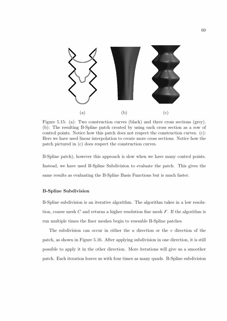
60

(a) (b) (c)

Figure 5.15: (a): Two construction curves (black) and three cross sections (grey).(b): The resulting B-Spline patch created by using each cross section as a row ofcontrol points. Notice how this patch does not respect the construction curves. (c):Here we have used linear interpolation to create more cross sections. Notice how thepatch pictured in (c) does respect the construction curves.

B-Spline patch), however this approach is slow when we have many control points.

Instead, we have used B-Spline Subdivision to evaluate the patch. This gives the

same results as evaluating the B-Spline Basis Functions but is much faster.

B-Spline Subdivision

B-Spline subdivision is an iterative algorithm. The algorithm takes in a low resolu-

tion, coarse mesh C and returns a higher resolution fine mesh F . If the algorithm is

run multiple times the finer meshes begin to resemble B-Spline patches.

The subdivision can occur in either the u direction or the v direction of the

patch, as shown in Figure 5.16. After applying subdivision in one direction, it is still

possible to apply it in the other direction. More iterations will give us a smoother

patch. Each iteration leaves us with four times as many quads. B-Spline subdivision

61

is a simple algorithm:

Fj =1

2∗ Ci +

1

2∗ Ci+1

Fj+1 =1

8∗ Ci−1 +

3

4∗ Ci +

1

8∗ Ci+1

Where the step size of i is one, and the step size of j is two. This equation is the

general case of subdivision and needs to be slightly modified for the end cases of the

subdivision.

We have used a simple interface used to control the subdivision parameters,

and this is described in Appendix A. Subdivision parameters include the number of

subdivisions in each direction. It is also possible to control the number of evaluations

in the u and v directions via the same interface.

62

(a) (b) (c)

(d) (e)

Figure 5.16: (a): A control mesh for a B-Spline patch. (b): A B-Spline patch createdfrom subdividing the control mesh once in the u direction. (c): The patch after onesubdivision in the v direction. (d): The patch after two subdivisions in the u and vdirections. (e) A gouraud shaded version of the patch shown in (d).

Chapter 6

Editing Phase

In the editing phase, the user can modify the model that he/she constructed in the

creation phase. This fits very well with the artistic design process of progressive

drawing refinement, which is particularly prevalent in various sketching techniques

(Section 1, Figure 1.1). We are free to use parametric or mesh representation at the

editing stage. Consequently, any technique for mesh editing can be also employed

here [LF03, VSMM00, ZSS97]. However, we prefer to use the stroke based parametric

representation again, which is consistent with our creation phase. This allows us to

design editing operations that complement our creation phase. In addition, it enables

us to keep the advantages of parametric representation, as we discussed in Chapter 4.

The next sections focuses on describing two major parametric editing methods which

are crucial for our system.

6.1 Orthogonal Deformation Stroke

This first technique of the editing phase was inspired by the traditional bending

(or distortion) method (Chapter 1, Figure 1.1). In this method, the artist adds

variations to the overall 3D shape of the subject by distorting with few strokes

its outlined form [DGK99]. Next, we describe how our approach approximates the

traditional bending method.

In the creation phase, the user specifies the surface with strokes by 2D drawing

63

64

Figure 6.1: The orthogonal deformation stroke in action. (a) the surface we wish todeform; (b) its constructive curves ql(u), qr(u), the center curve c(u), and a crosssection of the surface tu(v); (c) the surface as viewed from the side, notice thatql(u), qr(u) and c(u) are all the same, straight line when viewed from this angle; (d)the deformation stroke d(u); (e) the cross section and the strokes morphing to thedeformation stroke (the camera angle has been slightly altered for clarity); (f) thefinal, deformed surface.

operations in the xy plane. This helps the user to have a natural drawing feeling

while using our system, very similar to traditional pen-and-paper drawing. However,

the drawback to the advantage of drawing on a 2D piece of paper is on the lack

of flexibility for editing our models in the third dimension. In order to solve this

problem, we propose a mechanism to allow the user to deform the model in a direction

orthogonal to the drawing plane.

We begin by rotating the model so that we can see it from the side. Let ℘′ be the

new view plane. Note that all three curves ql(u) , qr(u) and c(u) form an identical

vertical line segment l(u) in this plane. The user enters the deformation stroke d(u)

in ℘′ as illustrated in Figures 6.1 and 6.2. From the user perspective, this stroke

shows the skeleton (the axis) of the deformed surface.

Based on our discussion in Chapter 5, the original surface S(u, v) is formed by

65

moving the cross section curve tu(v) along c(u) (see Figures 5.4 and 6.1). Note

that this is true for both surfaces of the creation phase. We use the deformation

stroke d(u) to transform cross sections of S(u, v) to a new set of curves that create

the deformed surface S(u, v). More specifically, for every fixed u, we transform

the cross section curve tu(v) to a new curve tu(v). The appropriate transformation

is determined by the relative situation of c(u) (or l(u)) and d(u) in the new view

plane ℘′. For this, let (l(u), Tl(u), V ) denote the source frame formed at l(u). In

this notation, Tl(u) is the unit tangent vector of l(u) and V is the view vector.

The destination frame is (d(u), Td(u), V ), where Td(u) is the unit tangent vector of

d(u). Let M(u) be the transformation that maps the source frame to the destination

frame for every u. Consequently, for each u, M(u) is a 4x4 transformation matrix

consisting of a translation and a rotation. If we assume that both tu(v) and tu(v)

are represented in the homogeneous coordinate system, then we have

tu(v) = M(u)tu(v) (6.1)

Again by changing u, the resulting curves tu(v) construct the deformed surface

S(u, v) as illustrated in Figures 6.1 and 6.2.

6.2 Cross Sectional Oversketch

This second technique of the editing phase is related to the traditional scribble

method (Chapter 1, Figure 1.1), in a similar way as described for cross sectional

blending surfaces (Section 5.4).

In our system, the user defines the cross section strokes in the drawing plane ℘.

66

Again, this fits the artistic approach for depicting 3D forms (Section 1, Figure 1.1).

This assumption is a good selection for the default objects. However, there is a

certain limitation due to the 2D mode of interaction. For example, it is hard to

control the behavior of the cross section curve near to the intersections.

We have designed a simple method that allows the user to change the cross section

stroke for any view. In this method, the user can rotate the object and change the

view, and then he/she can select a cross section on the surface. This is done by

setting the parameter u (Section 4.1) proportional to the mouse position. Then we

highlight the corresponding cross section tu(v) on the surface that forms a visible

interaction. At this stage, we map the changes given by the user to the cross section.

This is an operation that allows the user to edit a surface by oversketching. As shown

in Figure 6.3, we simply insert the new portion of the stroke, and delete the old one.

67

Figure 6.2: Left: perspective view of three deformation strokes (in white) appliedto the single leaf model of Figure 5.7. Right: artistic composition using our systemillustrating the shape and color progression of autumn leaf. The stem was modeledas a rotational blending surface. The leaf of Figure 5.7 is placed at the top of thestem. The other three leaves are deformations of this top leaf using three differentorthogonal deformation strokes.

68

Figure 6.3: A skirt modeled with cross sectional oversketch. Top row, left to right:starting with a simple tube, the user selects a cross section of the surface. Next,the user redraws a section of it and this edits the surface. Bottom row: the surfaceis rotated and drawn upon further, and the results are shown with both toon andGouraud shading for clarity.

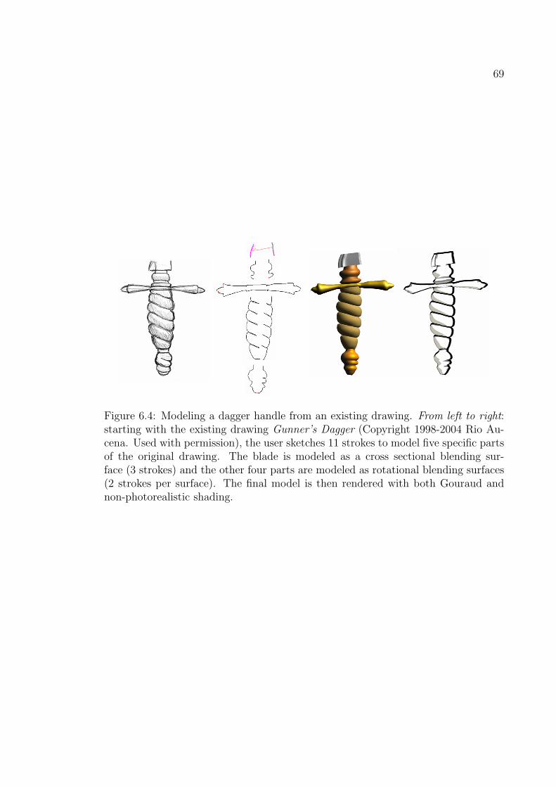
69

Figure 6.4: Modeling a dagger handle from an existing drawing. From left to right:starting with the existing drawing Gunner’s Dagger (Copyright 1998-2004 Rio Au-cena. Used with permission), the user sketches 11 strokes to model five specific partsof the original drawing. The blade is modeled as a cross sectional blending sur-face (3 strokes) and the other four parts are modeled as rotational blending surfaces(2 strokes per surface). The final model is then rendered with both Gouraud andnon-photorealistic shading.

Chapter 7

Rendering Phase

Rendering is important in every modeling system. This is because the user must be

given feedback during the modeling process. Feedback should depict the shape of

the model so that it is visually apparent. In order to keep our system interactive,

we designed the rendering to run in real-time. Because of this, efficiency becomes a

key factor when deciding on what rendering algorithm to use. Apart from regular

Gouraud shading (a default in OpenGL), our system allows the user to render in two

styles (Section A.2.1 shows how to select a rendering style), toon shading (Section

7.1) and a line shading system we developed which is called HBED (Hardware Based

Edge Detection, Section 7.2). For an example of the non computer generated art

upon which these rendering styles are based on, see Figure 7.1.

7.1 Toon Shading

The default rendering style in our system is toon shading [LMHB00], as pictured in

Figure 7.2. This has been chosen as the default renderer because toon shaded models

seem less imposing and more accessible, and because many of our models tended to

be cartoon characters. Toon shading works similarly to standard Gouraud shading.

Recall Phong’s lighting equation:

I = IaKa +m∑

i=1

Ii(Kd(L ·N) + Ks(R · V )n) (7.1)

70

71

(A) (B)

(C) (D)

Figure 7.1: (A): Cel (AKA toon) shaded art from an animated cartoon, Bug inMouth Disease (Copyright Homestar Runner). (B): Cel shaded art promoting theanimated series, Cowboy Bebop (Copyright Columbia TriStar). Our toon shader isbased on the type of cel shading shown in (A) and (B). (C): Line art, from [Loo43].(D): Ink, wash, and chalk drawing by the Renaissance master Cambiaso [Hal83].Our HBED renderer is based on the types of art shown in (C) and (D).

72

(a) (b)

(c) (d)

Figure 7.2: Comparison between two shading models, (a) Gouraud, (b) toon. Al-though the two shading models are mathematically similar, the toon shaded modelsare aesthetically different. Cartoons do not seem imposing and add to the feelingof accessibility. Also, the hand drawn nature of sketch based modeling seems to fitbetter with toon shading.

73

Here we assume some familiarity with Phong’s equation but we will briefly go

over the various parts of Equation 7.1. Phong’s lighting equation can be broken up

into three parts; ambient, diffuse and specular. The specular part is IaKa. Ia is the

color of the ambient light, which is constant throughout a scene. Ka is the ambient

color of the surface we are shading. The diffuse and specular components work a bit

differently, they are added in for each of the m lights present in the scene. This is the

source of the summation in Equation 7.1, and each individual light is represented

as Ii. The diffuse portion is Kd(L · N). Kd is the diffuse color of the surface we

are shading. L is the light vector, or the direction from the point we are shading to

Ii. N is the surface normal of the point we are shading. Finally, the specular part

is Ks(R · V )n. V , the view vector, is the vector from the point we are shading to

the viewer’s eye. To avoid recalculating this for each pixel, the view vector can be

approximated as the constant value < 0, 0, 1 >. The specular color of the surface we

are shading is Ks. R is the reflection vector, or the way the light from Ii will reflect if

the surface was a perfect reflector. This is computed as R = 2N(L ·N)−L. Finally,

we have the specular exponent n. Having a higher value for n results in a more

concentrated highlight, and makes a surface look more shiny. By convention, all

dot products in Phong’s equation are clamped to the range [0, 1], as this eliminates

negative colors.

Phong’s equation can be reduced to an equation of two variables:

I = F (x, y) (7.2)

74

(a) (b)

Figure 7.3: (a): A plot of Equation 7.1 over the entire [0, 1] domain. (b): A thresh-olded version of Equation 7.1.

Where x = N · L and y = (R · V )n. Recalling that we usually clamp all dot

products in Phong’s equation so that they fall in the range of [0, 1], we see that x

and y both fall in the range [0, 1]. Figure 7.3 shows a plot of the function F . By

thresholding x and y from equation 7.1, we can arrive at toon shading. A thresholded

plot of F is also shown in Figure 7.3.

Toonshading: Choosing Threshold Values

As stated in the Section 7.1, toon shading applies thresholding (discretization) to

the dot product of N and L during the diffuse calculation, and applies thresholding

to the dot product of R and V during the specular calculation. Each threshold range

is mapped to an intensity value, which then gets multiplied by the material color, as

in Phong lighting.

75

For toonshading, the only thing we can really adjust are the threshold ranges,

and the color that each range gets thresholded to. There is no universally correct col-

lection of threshold ranges, and for optimal visual effectiveness the threshold ranges

must be tweaked for each 3D model. However, through experimentation, it is possi-

ble to find a collection of threshold ranges that works well in most cases. The Utah

teapot exhibits a good range of contours with which to test threshold ranges. Using

the Utah teapot and other models, we came up with the threshold ranges in Figure

7.4 and Figure 7.5.

7.2 HBED: Rendering as Lines

The second type of rendering in our system is called HBED (Hardware Based Edge

Detection). HBED renderings look similar to an actual drawing (see Figure 7.6).

It makes sense in a sketch based modeling system to render in the style of an ac-

tual sketch. Additionally, rendering as lines gives us a good sense of the overall

shape of the object, and especially of the overlapping forms and creases. HBED is

implemented using GPU programming (see Appendix C).

Rendering using lines alone has been a recurring goal in non-photorealistic ren-

dering. There are many approaches to this, and some focus on realtime generation

of lines. The HBED approach is essentially a GPU based version of the approach

outlined by Green et. al. in [GSS+99]. HBED is a two pass method. The first pass

renders the surface normals and depth values of the scene into a temporary buffer,

while the second pass uses this buffer to find out how to render the scene as a line

drawing.

76

range of N · L value thresholded to[−1.0, 0] 0[0, .1] .1[.1, .2] .3[.2, .7] .5[.7, 1.0] .7

(a) (b)

(c) (d)

Figure 7.4: Diffuse thresholding. (a): The left column of the table shows the value ofthe dot product between the normal vector and the light vector. The right column ofthe table shows what each range of dot products is thresholded to. (b): Two ramps,the top ramp shows diffuse color values without thresholding and the bottom showsdiffuse color values with thresholding. (c): Teapot without thresholding applied.(d): Teapot with thresholding applied.

77

range of R · V value thresholded to[−1.0, .8] 0[.8, 1.0] 1

(a) (b)

(c) (d)

Figure 7.5: Specular thresholding. (a): The left column of the table shows the valueof the dot product between the normal vector and the light vector. The right columnof the table shows what each range of dot products is thresholded to. (b): Two ramps,the top ramp shows specular color values without thresholding and the bottom showsspecular color values with thresholding. (c): Teapot without thresholding applied.(d): Teapot with thresholding applied.

78

(A) (B)

Figure 7.6: The handle of a dagger. (A): The handle as drawn by an artist. (B):The handle as rendered with HBED. Notice the similarity to (A).

Figure 7.7: Here we see two different renderings of the same seashell. The image onthe left has been gouraud shaded, while the one on the right has been rendered inHBED. The right image is definitely easier to make out.

79

7.2.1 HBED: The First Pass

The first pass of HBED renders the scene into a temporary buffer. This buffer is

called the p-buffer. This buffer is similar to the frame buffer, but there are three key

differences. First, the frame buffer is displayed on the monitor, while the p-buffer

remains hidden from view. Second, once the p-buffer is rendered, it is retained in

VRAM (video ram, which exists on the video card) as a texture map, which can be

used later in the same way as a regular texture map. Finally, while the frame buffer

contains three channels, red, green, and blue, the p-buffer contains four channels.

These four channels can be referred to as red, green, blue, and alpha. On most

modern video cards, each channel is a 32-bits wide and is intended to hold a floating

point number.

Normally in computer graphics, each triangle is shaded using Phong’s lighting

model. In a programmable GPU, we can use any program or lighting model we want

to shade each triangle. In the first pass, we render the surface normal to the red,

green, and blue channel of the p-buffer. We render the depth value, which we have

after the so-called perspective divide, into the alpha channel. This is shown in Figure

7.8.

Texture maps store values which range from zero to one. The x, y, and z com-

ponents of a surface normal range from -1 to +1. Therefore, the surface normal N

will have to be normalized to the range [0, 1] during the first pass. Z-Buffering must

be enabled during the first pass for purposes of hidden line removal.

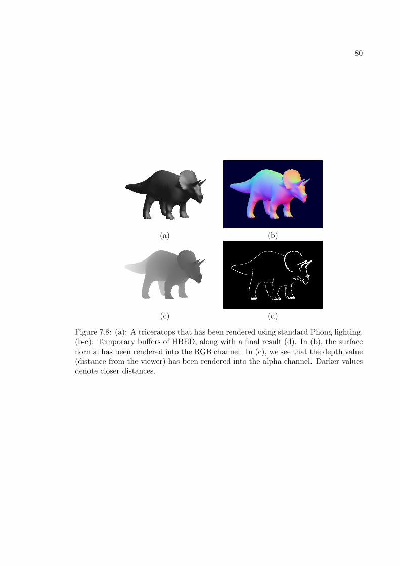
80

(a) (b)

(c) (d)

Figure 7.8: (a): A triceratops that has been rendered using standard Phong lighting.(b-c): Temporary buffers of HBED, along with a final result (d). In (b), the surfacenormal has been rendered into the RGB channel. In (c), we see that the depth value(distance from the viewer) has been rendered into the alpha channel. Darker valuesdenote closer distances.

81

7.2.2 HBED: The Second Pass

The second consists of rendering just one primitive to the screen; a single quad.

This quad is exactly the same size as the entire screen, and is texture mapped with

the p-buffer. Instead of just displaying the RGBA data of the texture map at each

pixel, a shader program is applied at each pixel. This shader program subtracts the

normal and depth values of the current pixel from its neighboring pixels. If either

the difference of the surface normals or of the depth values is high enough, it renders

a black pixel (or white, or whatever color you want the line to be). Otherwise, it

renders nothing at all. It is possible to render nothing at all in a shader by using the

discard command. After performing this simple subtraction, we can get the results

in Figures 7.7 and 7.8. Our results were generated by using a threshold of .15 for

surface normals, and a depth threshold of .05 (in normalized device space). Figure

7.10 shows several image processing operators, which is another way to picture the

subtraction of the normal and depth values between adjacent pixels. These operators

are called Kernels and are common in image processing [Pit00].

7.2.3 Efficiency of HBED

The first pass of HBED is straightforward. The second pass also is very efficient.

Since the main computation in the second pass is a pixel subtraction, and we always

have the same number of pixels in a window, the number of polygons in a scene

doesn’t affect the running time the second pass. This is a powerful and important

property that is shared by all pixel shaders.

82

7.2.4 Stylization of HBED

There are several ways to stylize HBED. First, it is possible to exchange the basic

image processing kernels to kernel D in Figure 7.10. This gives results similar to

the ones shown in Figure 7.6. The kernel is not symmetrical, and this also causes

the lines to be different widths at different angles, which is also what happens when

drawing with an ink brush or certain kinds of markers.

Another way to stylize HBED is by looking at the way the thresholding is done.

The range of differences between two pixels’ normals can be mapped to various grey

values. The highest difference, for instance, can be solid white while a very small

difference can be very close to black, and everything in-between these can be a

continuum of grey values.

A third way to stylize HBED is by utilizing the fact that we have the surface

normals in the second pass. Surface normals are the basis for almost all lighting

equations in computer graphics, so many of the most popular lighting styles are also

compatible with HBED. For instance, it is possible to apply toon shading or phong

shading.

Finally, a fourth way to stylize HBED is to composite the HBED line image onto

a picture of a piece of paper. This gives the illusion that your drawing is coming to

life in full 3D. Figure 7.9 shows a pear rendered with all these stylizations.

83

(a) (b) (c)

Figure 7.9: (a): A stylized pear rendered using a modified HBED system. HBEDhas been modified to also include some toon shading to simulate an ink wash. Theimage was composited onto a picture of a piece of hand made, slightly colored paper.Kernel D in Figure 7.10 was used. (b): A pear rendered using Kernel C in Figure7.10 HBED approach. (c): For contrast, we show a phong shaded pear here.

0 −14

0−14

1 −14

0 −14

0

0 0 −14

0 00 0 0 0 0−14

0 1 0 −14

0 0 0 0 00 0 −1

40 0

Kernel A Kernel B

0 −12

00 1 −1

2

0 0 0

0 0 −12

0 00 0 0 0 00 0 1 0 −1

2

0 0 0 0 00 0 0 0 0

Kernel C Kernel D

Figure 7.10: The image processing kernels used in HBED. Each number representsa pixel’s weight. Kernel A is used when rendering lines in a style similar to thatin Figure 7.7. Kernel B is used when rendering lines in a style similar to that inFigure 7.6. Since Kernels A and B have four nonzero values in them, the each requirefour lookups into texture memory per pixel. Kernels C and D are similar to A andB respectively, except C and D only require two lookups into texture memory. Cand D are very good approximations to A and B, and they are much faster, so ourimplementation uses C and D.

Chapter 8

Results and Discussion

In order to generate the results, we created a prototype sketch system. The system

was programmed from scratch in C++. It consisted of around 22,000 lines of code

and comments according to the CCCC code profiler, which can be found at

www.sourceforge.net/projects/cccc. The prototype system incorporated about 40

C++ objects. The ratio of lines of code to lines of comments was 3:1. All the results

were generated on an AMD Anthlon 2800 with a GeForce 5900 XT, 512 MB card,

with quad meshes from our parametric representation rendered in OpenGL. GPU

programming was used for shading purposes (See Appendix C and Chapter 7).

We created 3D models using few strokes representing subjects of cartoon styles

(Figures 5.5, 5.8, 6.3, 6.4, 8.1, 8.2) and botanical illustrations (Figures 5.7, 6.2, 8.5, 8.6).

We were able to construct models with sharp corners (i.e. candle in Figure 5.5), facets

(i.e. sword in Figure 5.8), and bumps (i.e. pumpkin in Figure 8.1). We have also cre-

ated models with multiple cross sections. Figures 8.3 and 8.4 detail the construction

of a some multiple-cross section based models.

We observed that, in many cases, some models such as the pear, candle, laser

gun, sword, leafy stalk, and pumpkin are particularly fast to create (around less than

a minute) using rotational and/or cross sectional blending surfaces. More complex

models took longer because they relied more upon the assembly of parts (fitting each

surface together). However, our research focused on steps of the modeling rather than

the assembly process. Therefore, we implemented standard techniques for assembling

84

85

3D parts, in which the user directs translation and rotation by clicking and dragging

with the mouse, in a way based on translation in Maya (see Section A.3). We found

this kind of assembly interface to be the major bottleneck of our creative process.

When creating models of the wizard, Vulpix, and the bad guy (Figures 8.1 and 8.2),

and for the yellow berries (Figure 8.6), over 60% of the time was spent on assembling

the parts. The wizard took about an hour to create, of which about 35 minutes were

spent assembling the parts. Clicking and dragging each surface so that it fit exactly

right with the other surfaces was tedious and difficult to do with the mouse or pen.

The yellow berries took around two hours to create with approximately 80 minutes

spent on assembling the leaves and berries to the stem. This shows that the assembly

process requires further streamlining and is in need of a new kind of interface, perhaps

sketch- and/or rule-based.

We also noticed that we were able to create many of our models more quickly than

we could have hand-drawn and shade the same objects. For instance, the constructive

lines (contour) of a pear took the same amount of time on computer as on paper, but

the computer-generated pear is quicker to create because it is automatically shaded,

for instance using the default Gouraud shading. A drawing done by hand has to

be shaded manually, for instance using the side of the pencil or hatching. This

automatic shading is notable because it usually takes longer to model something

on a computer than to sketch it on paper. This is one of the reasons artists draw

“concept sketches” on paper rather than “concept models” on a computer. On the

other hand, some extremly proficient artists can model faster than they can draw;

this is an exceptional skill and is only true for certain types of models.

86

Figure 8.1: Cartoon-like shapes. From top to bottom with total number of strokessketched by the user in parenthesis: paprika (2) and tangerine (2) (both sketcheddirectly over the spiral method drawings in Figure 1.1), pumpkin (5), bad guy (19),Wizard (57), and snoopy (10).

87

Figure 8.2: Cartoon-like shapes. Vulpix, a cartoon fox took 13 strokes to make, whileOddish, a cartoon radish, took 15.

88

(A) (B)

(C) (D)

Figure 8.3: The construction of a spaceship, which has multiple cross sections. Thefinal ship is in (A). The nosecone, rocket, and cockpit consist of rotational blendingsurfaces, but the body (B) needs multiple cross sections, and in our system this makesit a B-Spline patch. The strokes used to create this B-Spline patch are shown in (C).Black strokes are the construction curves, while red ones are the cross sections. (D)shows the body of the ship from the same view as (C). Note that the cross sectionsin (C) are very different from each other.

89

(A) (B)

(C) (D)

Figure 8.4: The construction of a fish. The final fish is in (A). We see the fish’s headin (B), this portion will require multiple cross sections, and in our system this makesit a B-Spline patch. The strokes used to create this B-Spline patch are shown in (C).Black strokes are the construction curves, while red ones are the cross sections. (D)shows the head of the fish from the same view as (C). The cross sections in (C) hadto be different from each other to make the fish’s nose stick out.

90

Figure 8.5: Rose, modeled in 23 strokes. The petals and the three stems were gen-erated in 2 strokes each using rotational blending surfaces. Each leaf was generatedwith 3 strokes using cross sectional blending surfaces (Figure 5.7), distorted (Sec-tion 6.2) and interactively placed at the stem using standard rotation/translationmodeling tools similar to the ones found in Maya [Aut06]. Bottom image: (left) thetwo strokes sketched for the rose petals; (middle and right) real botanical illustra-tions were used as templates for sketching over the leaves (two middle leaves [Wes83]and a sample from a painting).

91

Figure 8.6: Pyramidalis Fructu Luteo (yellow berries), modeled in 33 strokes. Theberries and the stem were generated in 2 strokes each using rotational blending sur-faces. Each leaf was generated with 3 strokes using cross sectional blending surfaces(Figure 5.7). Bottom left image: The user sketched directly over nine specific partsof a real botanical illustration of yellow berries (Copyright 2004 Siriol Sherlock. Usedwith permission.): one stem, three leaves and five berries (right image). In the model,all leaves and berries are instances of these nine sketched-based objects. Each of theleaf instances was properly distorted (Section 6.2) and both leaves and berries werethen placed at the stem by the user with standard modeling tools.

Chapter 9

Conclusions

This thesis presented a novel sketch-based system that allows interactive modeling

of many free-form 3D objects with few numbers of strokes. Our technique draws on

conventional drawing methods and workflow to derive interaction idioms that should

be familiar to illustrators. We have developed algorithms for parametric surfaces

using rotational and cross sectional blending, as well as a novel technique for sketch

based design of B-Spline patches. Although we were inspired by traditional pencil

and paper drawing techniques, our methods allow either subtle or incremental (as

with paper) or large-scale changes to the objects. Overall, we have made progress in

the realm of sketch based modeling.

Our results with cartoon-like features show that it is possible to model quite con-

voluted shapes with a small number of strokes. This differs from classical animation

systems that require lots of menu selections and data entry to accomplish even the

simplest tasks.

We tackled all of the main aspects that a sketch based system should have, from

the ground up. Our stroke capture method is efficient and leads to a B-Spline, which

is suitable for 2D or 3D design. The stroke capturing method yields the control

points that are used in most other systems, so it is highly compatible with existing

methods.

We described several flexible new parametric surfaces that allow the user to model

3D objects quickly and easily. Although our surfaces are designed specifically for

92

93

sketch modeling, they could be used in other modeling applications. They could

even be integrated into existing modeling systems. These surfaces yielded good

results presented in chapter 8, and were efficient enough to run in real-time.

When combined with our editing operations, the parametric surfaces can be used

to design an even greater range of shapes. Our editing operations were specifically

designed to complement our parametric surfaces. Although they are tied somewhat

to our parametric definitions, similar editing operations could be devised that operate

under the same principle for other types of surfaces.

Our rendering system HBED (see Chapter 7) was used to bring the system even

further into the realm of the drawing by making the 3D models look like certain

styles of line art. HBED works seamlessly with the rest of the system because it is

efficient enough not to slow things down, and since it keeps the surface normals, it

could be combined with other rendering algorithms in the future. For instance, it

would be easy to merge HBED with toon shading.

There are many avenues for future research. Sketch based modeling techniques

can be combined with commercial packages. In the case of Maya, this would be

implemented by writing a plugin. After such a plugin was implemented, the sketching

process could further be refined by observing how sketch modeling compliments other

types of modeling. More typical modeling techniques could be modified so that they

fit better with sketch modeling, and vice versa.

Another direction of research would be to learn more drawing rules from artists

and define new parametric surfaces or editing operations based on these drawing

rules. Using the framework of this thesis, this would be adding more and/or better

options to the creation and editing phases. Learning drawing rules from artists would

94

probably require collaborative research with artists.

As with any new method of human-computer interaction, a series of user studies

needs to be carried out. The user base would have to be artists. It would be

interesting to know what artists who have never used a 3D modeling program thought

of our sketch modeling system, and also what artists who have used other commercial

packages thought of it. It would also be important to measure how fast an artist

could learn to use our sketch system versus how long it takes an artist to learn the

various commercial packages.

In this thesis, we were able to develop new types of parametric surfaces that

were made to fit in with our sketching operations. If new sketching operations are

developed, new types of surfaces might also have to be developed. These new surfaces

could have features missing from our current system, such as the ability to branch.

Another good feature would be the ability to blend with nearby surfaces much as

an implicit surface can, and yet another good ability would be parametric surfaces

specifically designed for efficient sketch based CSG operations.

Another interesting prospect would be to re-invent the graphics pipeline itself in

a way more related to drawing. Generally speaking, the rendering phase is separate

from the modeling phase. But in a drawing, there is often no distinction from

rendering and geometry. For instance, shading an object on paper helps define

its form, while in 3D graphics the form of an object is defined by the location

of its vertices and shading is a separate step from defining the vertex positions.

Having more interdependence between rendering and geometry is difficult to picture

mathematically, but it definitely is an avenue of research that needs to be tackled.

Finally, sketch based modeling needs to be formally compared and contrasted

95

with another competing metaphor for 3D design: sculpting based modeling. Sculpt-

ing based modeling tries to simulate the traditional method of designing 3D objects,

sculpting, for instance out of marble or clay. This method competes with that of

sketch based modeling. Yet perhaps sculpting could be combined with sketching in

some ways to create a hybrid system.

Appendix A

Interface

This section details the interface of our sketch based system.

A.1 General Operation

Left clicking and dragging creates a stroke. Right clicking and dragging rotates the

camera. Hitting the ‘control’ (CTRL) key on the keyboard while right clicking and

dragging pans the camera. Another way to rotate the camera is by using the middle

mouse button while dragging. This middle mouse button method rotates the camera

around the z-axis only.

A.2 Interface Elements

While the main goal of the system is to provide sketch based interaction, several other

methods of interaction are valuable for certain tasks. For example, when specifying a

file name it is much better to type in the filename via the keyboard than to somehow

try to sketch the filename. Because of this the system uses several different types of

interface elements for different purposes.

A.2.1 Menu Bar

Pulldown menus (Figure A.1) are standard fare in windows type applications. They

are useful when opening files or selecting between different modes of interaction, or

96

97

when adjusting other settings. The menubar in our system is almost the same as

the standard Windows menubar, ours was just re-coded for esthetic reasons. Our

menubar features these options:

Figure A.1: Left: A menu bar from a windows application. The menubar consists ofseveral pulldown menus. Right: The menubar in our system, which is based on thewindows style menubar.

• File Menu

– open This opens a 3D model file. We haven’t used any special file exten-

sions, so there are files like “pear”, “fish”, etc. Opening a file will clear

(erase) any existing model, load the model from a file you specify via the

keyboard, and center the file.

– save as This is the only way to save a file. After selecting save as

you must specify a file name via the keyboard. You can give it any file

extension you want.

– export obj Exports the current scene to an .obj file. The .obj file format

is a popular format that most modeling programs can read. It comes in

two varieties, binary and ASCII. This program uses the ASCII type. The

.obj file created will use the same coordinate system that the modeler

uses, so you may need to rescale the scene if you open it in a 3D modeling

package depending upon what coordinate system the package uses.

98

– exit This quits the program. You can also hit the ‘escape’ key to quit.

Please remember to save your file before exiting!

• Edit Menu

– undo Erases the last stroke that you entered. You can also use the ‘u’

hotkey.

– snap to grid Turns on or off grid snapping mode. When in grid snapping

mode, you left click each time you want to add another point to the stroke

you are drawing, and each point is snapped to the nearest grid line. Right

clicking ends the stroke.

– center scene Centers the current scene. This is easier than translating

each surface to the center of the screen manually.

– mirror h Mirrors the last stroke you drew horizontally (about the y-axis).

You can now place the stroke with the mouse. If you move the mouse,

the newly mirrored stroke moves with it. Left clicking places the stroke.

– mirror v Mirrors the last stroke you drew vertically (about the x-axis)

but is otherwise the same as “mirror h”

• View Menu

– fullscreen Makes the system take up the full screen of the monitor. The

hotkey ’f’ also does this. If the system is already in fullscreen mode, this

menu entry causes the system to become a normal window. This option

is recommended.

99

– fps Displays the FPS (frames per second) that the application is getting.

This is useful for debugging or when trying the system out on different

video cards.

– black background Changes the background color of the system to black.

Some users may prefer this to the default color, which is dark blue.

– blue background Changes the background color of the system to dark

blue. This is the default color.

– paper background Changes the background color of the system to re-

semble a piece of drawing paper.

– reset rotation If you’ve rotated the model, this menu option resets the

camera angle to the default angle. In mathematical terms this means that

it sets the camera quaternion to < 0, 0, 0, 1 >.

– reset pan If you’ve panned the camera, this gets rid of the camera pan

and returns the camera to its original position.

– poly count This displays the total of polygons your model has, it is the

sum of the number of polygons in each individual surface. The polygons

are all quads, so multiply this by two to get the triangle count.

– normals Shows the surface normals. This is useful for debugging.

– patch strokes Shows the strokes you used to create each surface. Useful

if you want to show how the 3D surface was constructed using strokes.

– subdivision editor This brings up the subdivision editor. See section

A.4 for more details.

100

• Render Menu

– gouraud Sets the shading to gouraud shading. This is the typical lighting

provided by OpenGL.

– phong Sets the shading to phong shading (via a shader).

– engraved Sets the shading to an NPR shader I wrote, but it doesn’t work

very well if the polygons are small.

– toon Sets the shading to toon (A.K.A. cell) shading, via a shader. This

is the default option of the system.

– metallic Sets the shading to a metallic style NPR shading (via a shader).

– HBED lines Sets the shading to resemble a line drawing. Doesn’t work

well for all window sizes due to driver limitations.

– HBED ink Sets the shading to resemble an ink and wash drawing.

Doesn’t work well for all window sizes due to driver limitations.

There is also a “brush” pulldown menu but since the brushing features aren’t

discussed in this thesis, explaining the “brush” menu would only complicate things.

A.2.2 Tapes

A tape is similar to a pulldown menu. When contracted, the tape appears as an

arrow (Fig. A.2), but when expanded it appears as a series of buttons. The tape

is convenient when the user hasn’t learned the hotkeys yet or if he forgets them,

but once the user learns the hotkeys for the various functions, it is easier to use the

hotkeys. There are two tapes used in the system, the mode tape and the lathe tape.

101

Mode Tape

The mode tape is situated in the lower left corner of the screen (shown in Figure

A.2. The mode tape contains several buttons:

• Freehand: This button is the default drawing mode. It allows you to create

rotational blending surfaces and pipe surfaces (Chapter 5). When you exit

another mode, you enter freehand mode. It is also the default mode.

• Lathe: This button allows you to create cross sectional blending surfaces and

B-Spline patches (Chapter 5). You can also use the hotkey ’l’ to enter this

mode.

• Select: This button enters selection mode, see Section A.3.

• Brush: This button is for a feature we will not discuss in this thesis.

Lathe Tape

The lathe tape appears on the screen only when you are in lathe mode. It is pictured

in Figure A.3. It has several buttons:

• As Front: This controls how your cross sectional surfaces or B-Spline patches

are made. When this option is selected, the surface is given a back portion

that resembles the the part you sketch, but is mirrored around the screen’s x-y

plane. This back portion gets connected to the front portion. See Figure A.4

• None: This is the default option. It creates surfaces without a back.

• User Defined: This option is reserved for future work.

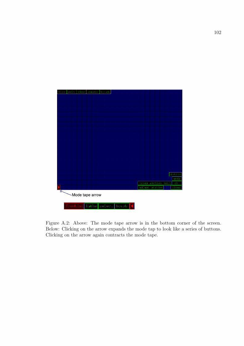
102

Figure A.2: Above: The mode tape arrow is in the bottom corner of the screen.Below: Clicking on the arrow expands the mode tap to look like a series of buttons.Clicking on the arrow again contracts the mode tape.

103

Figure A.3: Above: The lathe tape arrow is on the right edge of the screen. Below:Clicking on the arrow expands the lathe tap to look like a series of buttons. Clickingon the arrow again contracts the lathe tape.

Figure A.4: A B-Spline surface created from the strokes pictured to the left. Themiddle image shows this surface without a back, while the right image shows it witha back. The back of the surface mirrors the front of the surface exactly.

104

A.2.3 Hot Keys

The program uses many different hotkeys. It is often much faster to select an object

by hitting a single key on the keyboard rather then from a menu or button. Here is

a list of them:

• G: Show or hide the grid lines.

• P: Show or hide the paper texture map (when the background mode is set to

paper mode).

• W: Wireframe mode, turns a wireframe rendering mode on or off.

• Q: Increases the default radius of the pipe surface.

• SHIFT + Q: Decreases the default radius of the pipe surface.

• -: Makes the grid cells smaller.

• =: Makes the grid cells larger.

• SHIFT + =: Return to the default grid size.

• L: Enter lathe mode, which allows you to create B-Spline patches and cross

sectional surfaces.

• C: Deletes the last surface you made.

• E: Deletes all the surfaces (warning, this erases everything)

• F: Toggle fullscreen mode.

• N: Create a new surface after you have sketched the construction curves.

105

• U: Undo, erases the last curve you have sketched.

• Esc: Quit the program.

A.3 Selection Mode

This mode can be entered by using the mode tape from Section A.2.2. This mode

allows you to select and edit any or all of the surfaces. To select a surface, just click

on it. Next, a few new buttons will appear in the lower right part of the screen, as

shown in Figure A.5. The buttons allow us to perform various editing operations on

the surface:

• Bend: This allows you to run the orthogonal deformation stroke algorithm

from Section 6.1. When running the algorithm, additional buttons come on

the screen which allow you to confirm the deformation or undo it.

• Recreate: This button allows you to redefine a surface. The screen rotates

back to the camera angle which you used when drawing on the left and right

construction curves, as well as the cross section. Then, the program allows you

to draw on additional cross sections or get rid of existing ones, as well as to

redefine if you want the surface to have a back (as in Section A.2.2.

• Duplicate: This button creates a copy of the surface. It is useful, for example,

when designing a flower where the petals are all the same. You can just create

one petal, and duplicate it several times.

• Rotate: When you click the rotate button, the rotate panel pops up (see

Figure A.6. This allows you to rotate the surface.

106

• Translate: This button allows you to translate the surface by using the mouse.

A translation interface is shown over the surface (see Figure A.7). This interface

consists of three arrows and a yellow square. The arrows can be clicked and

dragged to move the surface around the x, y, and z-axis, while the yellow square

allows you to move the surface around in the directions of the view plane.

• Ambient, Diffuse, Specular: This allows you to change the ambient, diffuse,

or specular color of the surface via the color sliders. The red slider changes the

red color component, the green and blue sliders act similarly. When changing

the specular color, a white slider also appears. This changes the specular

exponent of the surface (the size of the highlight).

• More... The “more...” button brings up the extended color dialogue, which is

pictured in Figure A.8. This brings up a number of lit spheres. These spheres

are all colored differently. Clicking on a sphere changes the color of the surface

to match that of the sphere. This is often more convenient than using the color

sliders.

A.4 Subdivision Editor

The subdivision editor, pictured in Figure A.9, is used for controlling subdivision

parameters and other mesh parameters. When we create B-Spline patches, we use

subdivision (see Section 5.5.2). Here, we can control the number of subdivisions in

the two parametric directions (x and y, which are sometimes written as u and v),

as well as the relative size of the control mesh in these directions. The control mesh

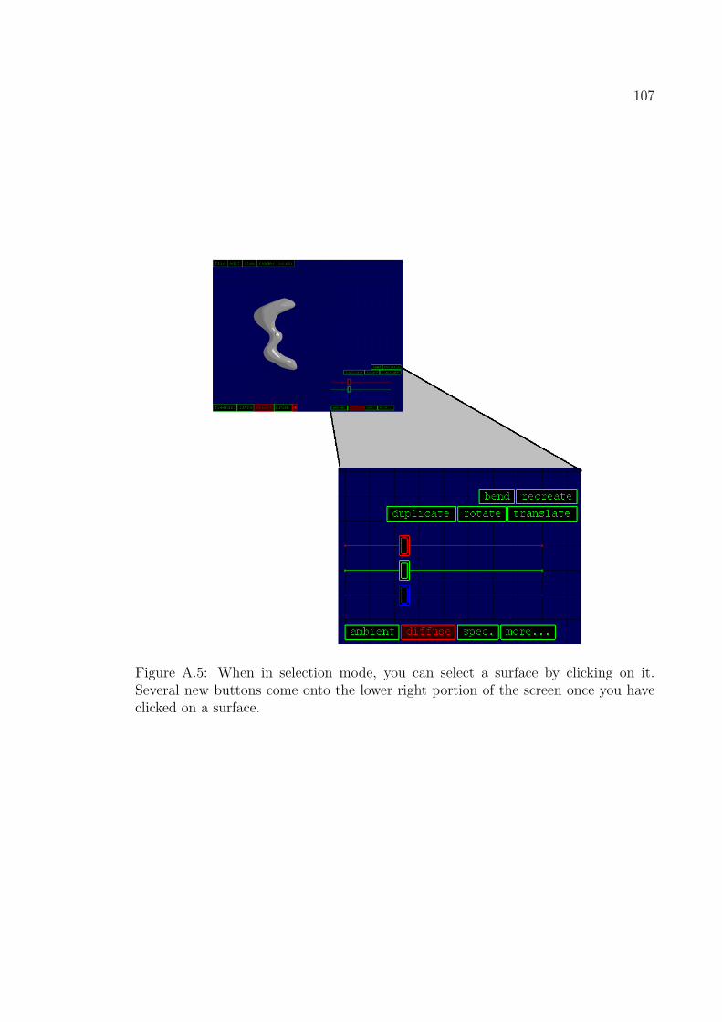
107

Figure A.5: When in selection mode, you can select a surface by clicking on it.Several new buttons come onto the lower right portion of the screen once you haveclicked on a surface.

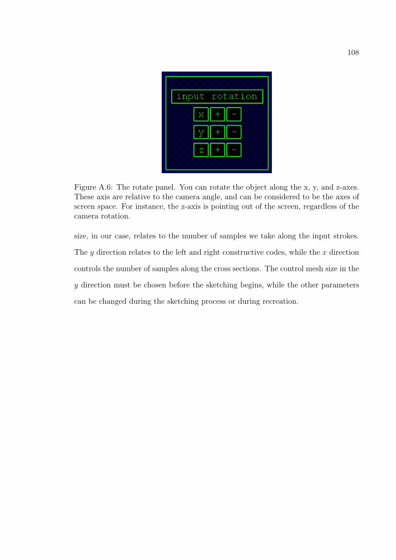
108

Figure A.6: The rotate panel. You can rotate the object along the x, y, and z-axes.These axis are relative to the camera angle, and can be considered to be the axes ofscreen space. For instance, the z-axis is pointing out of the screen, regardless of thecamera rotation.

size, in our case, relates to the number of samples we take along the input strokes.

The y direction relates to the left and right constructive codes, while the x direction

controls the number of samples along the cross sections. The control mesh size in the

y direction must be chosen before the sketching begins, while the other parameters

can be changed during the sketching process or during recreation.

109

Figure A.7: The translation interface. The red arrow can be clicked and dragged tomove the surface around in the direction of the x-axis. The green and blue arrowswork for the y and z-axis, respectively. The yellow square allows you to translatearound in the view plane, and is often more useful than the arrows.

110

Figure A.8: The extended color dialogue. Clicking on a sphere changes your surface’scolor properties so that the surface’s lighting resembles that of the sphere. This isoften more convenient than changing the color via one of the color sliders, but thecolor sliders can be used to create colors that aren’t present in the extended colordialogue.

Figure A.9: The subdivision editor. When we create B-Spline patches, we use sub-division. Here, we can control the number of subdivisions, as well as the relative sizeof the control mesh, which is related to the sampling rate.

Appendix B

Pseudocode

This appendix gives pseudocode for some of the algorithms discussed in other chap-

ters.

B.1 Creation Phase

This section gives pseudocode for the algorithms described in Chapter 5.

B.1.1 Rotational Blending Surface

This pseudocode describes how to make a Rotational Blending Surface (Section 5.3).

Rotational Blending Surface(ql, qr)1 n← Find Plane Normal(ql, qr)2 u← 03 while u ≤ 14 do v ← 05 while v ≤ 2π6 do s0 ← ql(u)+qr(u)

2

7 s1 ← ||qr(u)− ql(u)|| × n8 pl ← Rotate Point About Line(ql(u), s0, s1, v)9 pr ← Rotate Point About Line(qr(u), s0, s1,−v)

10 t← v2π

11 p← (1− t) ∗ pl + t ∗ pr

12 Add Point To Mesh(p)13 v ← v + v STEP14 u← u + u STEP

This function creates a rotational blending surface, such surfaces are described

111

112

in Section 5.3. As input, the function takes in two strokes ql and qr, which are also

described in Section 5.3. On line 1, Find Plane Normal(...) finds the normal which

the input strokes ql and qr lie upon. Lines 8-9 call Rotate Point About Line(...),

which takes in four parameters. The first parameter is the point you wish to rotate,

the second and third are two points on the line you wish to rotate about (so s0

and s1 can define an axis of rotation), and the last parameter is the amount of

radians you wish to rotate by. Line 11 is the actual blending between ql and qr.

Add Point To Mesh(...) is how our final result, the point p, gets stored into a mesh

data structure for later use. One common later use would be when tessellating the

mesh into quads or triangles, or when calculating the surface normal at each p.

B.1.2 Cross Sectional Blending Surface

This pseudocode describes how to make a Cross Sectional Blending Surface (Section

5.4).

Cross Sectional Blending Surface(ql, qr, tu)1 u← 02 while u ≤ 13 do ttransformed = Align To Axis(tu, ql(u), qr(u))4 v ← 05 while v ≤ 16 do p = ttransformed(v)7 Add Point To Mesh(p)8 v ← v + v STEP9 u← u + u STEP

This function creates a cross sectional blending surface, such surfaces are de-

scribed in Section 5.4. As input, the function takes in two strokes ql and qr, and

113

a single cross section denoted tu. The function Align To Axis transforms the in-

put stroke tu so that it lines up with the line segment between ql(u) and qr(u).

This entails rotating and scaling the line segment tu(0)tu(1) so that it lines up with

ql(u)qr(u). The same transformation that lines up these two line segments can be

applied to each point in tu, and this gives us ttransformed.

B.2 Editing Phase

This section gives pseudocode for the algorithms described in Chapter 6.

B.2.1 Orthogonal Deformation Stroke

This section gives pseudocode for the algorithm described in Section 6.1.

Orthogonal Deformation Stroke(S(u, v), d(u))1 u← 02 while u ≤ 13 do sa = ||S(u + ∆u, 0)− S(u, 0)||4 sb = ||S(u, 1)− S(u, 0)||5 sc = sa × sb

6 view vec = Get View Vector()7 da = ||d(u + ∆u)− d(u)||8 db = view vec9 dc = da × db

10 sp = Unproject(S(u, 0))11 dp = Unproject(d(u))12 M = Get Frame Transform(sp, sa, sb, sc, dp, da, db, dc)13 v ← 014 while v ≤ 115 do p←M ∗ S(u, v)16 Add Point To Mesh(p)17 v ← v + v STEP18 u← u + u STEP

114

Orthogonal Deformation Stroke takes as input two parameters: a surface S(u, v)

and a deformation stroke d(u). Lines 3-11 create two coordinate frames, s, the

source frame, and d, the destination frame. sa, sb, and sc are the basis vectors

of the coordinate frame, while sp is the point upon which the frame is centered.

Similarly, da, db, and dc are the basis vectors of the destination frame and dp is the

point on which the frame is centered. The function Get Frame Transform creates a

matrix that transforms us from the source frame to the destination frame. Line 15

transforms a point in the original surface S(u, v) by the frame transform matrix M .

Add Point To Mesh(...) is how our final result, the point p, gets stored into a

mesh data structure for later use. One common later use would be when tessellating

the mesh into quads or triangles, or when calculating the surface normal at each p.

B.2.2 Cross Sectional Oversketch

This section gives pseudocode for the algorithm described in Section 6.2.

Cross Sectional Oversketch(a(u), b(u), S(u, v))1 P ← Find Plane Stroke Lies Upon(a)2 bprojected← Project Stroke To Plane(b, P )3 anew ← Insert Stroke Into Cross Section(a, bprojected)4 Cross Sectional Blending Surface(S(u, v)ql(u), S(u, v)qr(u), anew)

This function takes in three parameters: the stroke we have chosen to oversketch

a(u), the oversketch stroke the user has drawn b(u), and the surface we are overs-

ketching S(u, v. After the stroke b has been projected to lie upon the same plane

that a lies upon, we can insert bprojected into a (described below), and this yields

anew. Then, we simply redefine the surface by using our newly defined stroke, anew.

115

The Insert Stroke Into Cross Section(...) subroutine takes in two parameters,

both of which are parametric curves. Let us call the first parameter of Insert Stroke Into Cross Section

x(u) and the second y(u). The goal of the subroutine is to insert y into x, creating

a new curve z. The insertion process ends up replacing part of the x(u) with all

of y(u). First, we must look at the endpoints of the curve y, which are y(0) and

y(1). We can find the point on x which is closest to y(0), and call this point x(α).

Similarly, the place on the curve x which is closest to y(1) can be called x(β). Delete

the portions of the curve from x(α) to x(β) and insert the stroke y in its place. Then,

reparamterize the entire curve and we have z.

Appendix C

GPU Overview

The purpose of this chapter is to give a brief overview of what the GPU is and why

we use it. Also included is some sample GLSlang (shading language) code.

C.1 Reasons for using the GPU

Since my system is all about interaction, fast rendering is a necessity. The GPU is

good at fast rendering in a variety of styles. Since the GPU is programmable, we

can achieve various different effects. For instance, the ability to render in the same

style as a drawing is related to sketch modeling, and we use the GPU to this end.

There are other, CPU based algorithms such as the Edge Buffer approach, which

uses hashing to accelerate the process of edge detection but we have found the GPU

method to be very fast and effective, and it can combine with other types of lighting.

We also use the GPU for simple toon shading.

C.2 What is the GPU?

The GPU is a SIMD processor located on the video card. The native data type varies

per video card, but typically is an array of four 32 bit floats, or a Vec4. This is an

appropriate data type because it can be used to represent a homogeneous coordinate,

an RGB value, or a vector, all of which are common in computer graphics.

The instructions present on a GPU tend to be geared towards computer graphics.

116

117

For instance, there is an instruction to take the inverse square root of a number.

Though this seems like a strange instruction at first, consider its use in the context

of normalizing a vector.

Other instructions include various vector and matrix operations: dot product,

adding two vectors, multiplying a vector by a scalar, multiplying a vector by a

matrix, multiplying two matrices, and so fourth. These kinds of operations are also

useful in computer graphics.

The GPU has access to VRAM, which is the RAM located on the video card.

Entities such as the frame buffer, back buffer, and texture maps typically reside in

VRAM. However, on a programmable GPU, any sort of data structure can live in

VRAM, much as any kind of data structure can live in RAM, which can be accessed

by the CPU.

In addition to having instructions appropriate the computer graphics, GPUs tend

to exhibit two levels of parallelism. The first level is the SIMD instructions. The

second level is the parallel pipes. Modern GPUs can process many pixels at a time.

For instance, a GPU that can process 16 pixels at a time is said to have 16 parallel

pixel pipes. In computer graphics, the shading of each pixel can be done independent

to adjacent pixels, and the parallel pipes is simply a hardware setup that takes

advantage of this situation.

Finally, another feature that is possessed by GPUs is something called rendering

contexts. Much as we can render to the back buffer or front buffer in classic computer

graphics, we can also render to other, offscreen buffers on the GPU. These are often

called P-Buffers or render to texture targets, but they carry other names. These

offscreen buffers can then be used for a number of post-processing, image based

118

effects such as motion blur, depth of field, or edge detection. They can also be used

as texture mapping.

GPUs have many other features, literally hundreds. However, this is beyond

the scope of this thesis. For a complete listing, I recommend visiting the OpenGL

Extension Registry, available from OpenGL’s website. It gives a complete listing of

every available extension to OpenGL, and many of these are hardware related.

C.3 The Graphics Pipeline

Shaders are a key element of GPU programming, and in order to discuss shaders,

we must first discuss the graphics pipeline. Though everyone in computer graphics

is familiar with the pipeline, it still bears going over because different parts of the

pipeline are related to different types of shaders.

Figure C.1 shows the modern graphics pipeline. The Application Stage contains

your C++ code, including any graphics code such as OpenGL. From a pipeline point

of view, the main point of the Application Stage is to send triangles to the video

card. In OpenGL this is done by using functions such as glBegin(GL QUADS) or

glBegin(GL TRIANGLES) coupled with the glVertex* functions.

Associated with each vertex of every triangle are the so called Per Vertex At-

tributes. Each vertex must have a 3D coordinate, and this is one of its attributes.

Other common attributes include color, material, texture coordinates, and surface

normal. These are all bundled with every vertex and sent to the video card. Collec-

tively, this is called the 3D Triangles Stage.

Next, we have the Geometry Stage. This stage is applied to every vertex in the

119

Figure C.1: The modern graphics pipeline is broken up into these stages. This isa simplified look at the pipeline, more complicated versions are available and thesecan vary per video card.

scene. Typically, the vertex is multiplied by the modelview and projection matrices

so that they end up being in eye space. The color of the vertex can sometimes be

computed as well, using the normal of the vertex. After this stage is completed, we

are left with 2D Triangles.

The Rasterization Stage is next. This stage is applied to every triangle in the

scene. In this stage the triangles are rasterized (scan converted), and the per vertex

attributes are interpolated over the triangle using perspective correct interpolation

(CITE???). After this, they may be considered to be Pixel Attributes. Color of

the triangle is based on these interpolated attributes. For instance, the texture

coordinate may be interpolated, or the color may be interpolated if we aren’t using

texture maps. In this stage of the pipeline, the Texture Lookup occurs, which relies

upon the texture coordinates to look at a texture map residing in VRAM. Finally,

120

the Z-Buffer is used in this stage.

C.4 The Programmable Graphics Pipeline

On modern GPUs, two stages of the graphics pipeline are programmable (besides,

obviously, the Application Stage). The Geometry Stage and the Rasterization Stage

are both programmable. A program for the Geometry Stage is called a Vertex Shader,

and a program for the Rasterization Stage is called a Pixel Shader or sometimes a

Fragment Shader. A shader can be programmed to do things other than to shade,

so the name “shader” is misleading.

If a programmer doesn’t program his own shaders, the video card will follow one

of many default programs. For instance, a vertex program that implements Gouraud

shading is followed if you have GL LIGHTING turned on. There is another default

program for basic texture mapping, etc. A shader is always running, regardless of

weather the programmer is aware of it or is keen on GPU programming.

C.4.1 Shader Programming

There are several available languages to program shaders in. The CG language

is supplied by NVIDIA, however it works on non NVIDIA products. GLSlang is

the official OpenGL Shading Language, and is also known as GLSL. HLSL is a

language supplied by Microsoft, and is available with DirectX but it isn’t compatible

with OpenGL. ISL was developed by SGI, who wanted to create a RenderMan like

language that was compatible with OpenGL and with SGI video cards. It is also

possible to program in assembly language, though this isn’t usually as desirable, and

121

programs will be less portable.

I have programmed in CG, GLSLang, and in assembly language. Some think

that GLSLang will be the most dominant and compatible shading language in the

future, but only time will tell if this is correct. The work for my master’s project

was in GLSLang, though I optimized it in assembly when necessary.

C.4.2 What can you program?

The entire geometry stage and rasterization stage are programmable. These stages

are, in a sense, like functions. That is, they take in certain parameters and return

certain parameters. And like functions in C++, we can choose what they take in

and return, however there are some restrictions, which are discussed below.

The vertex shader can take in any vertex attributes. You can use built in at-

tributes such as the surface normal or the vertex position in object space, or you can

add your own attributes. These attributes are passed up to the video card during

the Application Stage using OpenGL-like function calls. The only restriction is that

you must supply some kind of vertex coordinate, though you may disregard this

information in the actual shader if you don’t need it.

Like a C++ function, the vertex shader needs to return something. It can work

on any variables that will later become pixel attributes. The only restriction is that

it must, at the very least return a 2D vertex coordinate.

The pixel shader works in a similar fashion. The only restriction is that it must

set the pixel color. It also can perform one or more texture lookups. This accesses a

texture map and looks at one or more of its pixels. The vertex shader, in contrast,

can not access texture maps on most video cards (except for the newest ones).

122

C.5 Code Examples

Note that a GPU using the OpenGL Shading Language (GLSL) requires both a

vertex shader and a pixel shader to run. This section gives some code examples of

both types of shaders. First, we show a vertex shader. Next, we show two different

pixel shaders that can be used with the vertex shader.

C.5.1 Vertex Shader

varying vec3 normal;

varying vec3 vertex_to_light_vector;

void main()

{

// Transforming The Vertex Position To ModelView-Space

gl_Position = gl_ModelViewProjectionMatrix * gl_Vertex;

// Transforming The Normal To ModelView-Space

normal = normalize(gl_NormalMatrix * gl_Normal);

// Calculating The Vector From The Vertex Position To The Light Position

vec3 light_source = vec3(1.0,1.0,1.0);

vertex_to_light_vector = normalize(light_source - gl_Position.xyz);

}

C.5.2 Phong Shader

varying vec3 normal;

varying vec3 vertex_to_light_vector;

uniform vec4 AmbientColor;

uniform vec4 DiffuseColor;

uniform vec4 SpecularColor;

uniform float Shininess;

void main()

{

// Defining The Material Colors

123

vec3 N;//normal but with a flipped z if necessary

N = normal;

if(N.z < 0.0)

N = -N;

vec3 eyeVec = vec3(0.0, 0.0, 1.0);

vec3 halfVec = normalize(vertex_to_light_vector + eyeVec);

// Calculating The Diffuse Term And Clamping It To [0;1]

float DiffuseTerm = clamp(dot(N, vertex_to_light_vector), 0.0, 1.0);

//calc specular term...

//float SpecularTerm = clamp(pow(dot(N, halfVec), Shininess), 0.0, 1.0);

float SpecularTerm = clamp(dot(N, halfVec), 0.0, 1.0);

SpecularTerm = clamp(pow(SpecularTerm, Shininess),0.0,1.0);

// Calculating The Final Color

gl_FragColor = AmbientColor*.25 + DiffuseColor

* DiffuseTerm + SpecularColor*SpecularTerm;

gl_FragColor.w = 1.0;

}

C.5.3 Toon Shader

varying vec3 normal;

varying vec3 vertex_to_light_vector;

uniform vec4 AmbientColor;

uniform vec4 DiffuseColor;

uniform vec4 SpecularColor;

uniform float Shininess;

void main()

{

// Defining The Material Colors

vec3 N;//normal but with a flipped z if necessary

N = normal;

if(N.z < 0.0)

N = -N;

124

vec3 eyeVec = vec3(0.0, 0.0, 1.0);

vec3 halfVec = normalize(vertex_to_light_vector + eyeVec);

// Calculating The Diffuse Term And Clamping It To [0;1]

float DiffuseTerm = clamp(dot(N, vertex_to_light_vector), 0.0, 1.0);

//calc specular term...

float SpecularTerm = clamp(pow(dot(N, halfVec), Shininess), 0.0, 1.0);

//thresholding the colors

if(DiffuseTerm < .1)

DiffuseTerm = .1;

else if(DiffuseTerm > .7)

DiffuseTerm = .7;

else if(DiffuseTerm > .20)

DiffuseTerm = .50;

else DiffuseTerm = .3;

if(SpecularTerm > .8)

SpecularTerm = 1.0;

else SpecularTerm = 0.0;

// Calculating The Final Color

gl_FragColor = AmbientColor + DiffuseColor

* DiffuseTerm + SpecularColor*SpecularTerm;

}

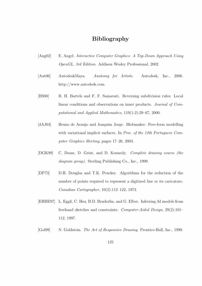
Bibliography

[Ang02] E. Angel. Interactive Computer Graphics: A Top-Down Approach Using

OpenGL, 3rd Edition. Addison Wesley Professional, 2002.

[Aut06] AutodeskMaya. Anatomy for Artists. Autodesk, Inc., 2006.

http://www.autodesk.com.

[BS00] R. H. Bartels and F. F. Samavati. Reversing subdivision rules: Local

linear conditions and observations on inner products. Journal of Com-

putational and Applied Mathematics, 119(1-2):29–67, 2000.

[dAJ03] Bruno de Araujo and Joaquim Jorge. Blobmaker: Free-form modelling

with variational implicit surfaces. In Proc. of the 12th Portuguese Com-

puter Graphics Meeting, pages 17–26, 2003.

[DGK99] C. Dease, D. Grint, and D. Kennedy. Complete drawing course (the

diagram group). Sterling Publishing Co., Inc., 1999.

[DP73] D.H. Douglas and T.K. Peucker. Algorithms for the reduction of the

number of points required to represent a digitized line or its caricature.

Canadian Cartographer, 10(2):112–122, 1973.

[EHBE97] L. Eggli, C. Hsu, B.D. Bruderlin, and G. Elber. Inferring 3d models from

freehand sketches and constraints. Computer-Aided Design, 29(2):101–

112, 1997.

[Gol99] N. Goldstein. The Art of Responsive Drawing. Prentice-Hall, Inc., 1999.

125

126

[GSS+99] Stuart Green, David Salesin, Simon Schofield, Aaron Hertzmann, Pe-

ter Litwinowicz, Amy Gooch, Cassidy Curtis, and Bruce Gooch. Non-

Photorealistic Rendering. SIGGRAPH 99 Course Notes, 1999.

[Gup77] A.L. Guptill. Rendering in Pencil. Watson-Guptill Publications, 1977.

[Hal83] R. Hale. Master Class in Figure Drawing. Watson-Guptill Publications,

1983.

[Ham63] J. Hamm. Drawing the Head and Figure. The Berkley Publishing Group,

1963.

[IC01] Takeo Igarashi and Dennis Cosgrove. Adaptive unwrapping for interac-

tive texture painting. In SI3D ’01: Proceedings of the 2001 symposium

on Interactive 3D graphics, pages 209–216, New York, NY, USA, 2001.

ACM Press.

[IH03] Takeo Igarashi and John F. Hughes. Smooth meshes for sketch-based

freeform modeling. In SI3D ’03: Proceedings of the 2003 symposium

on Interactive 3D graphics, pages 139–142, New York, NY, USA, 2003.

ACM Press.

[IMT99] T. Igarashi, S. Matsuoka, and H. Tanaka. Teddy: A sketching interface

for 3d freeform design. In Proc. of SIGGRAPH ’99, pages 409–416, 1999.

[IOOI05] Takashi Ijiri, Shigeru Owada, Makoto Okabe, and Takeo Igarashi. Floral

diagrams and inflorescences: interactive flower modeling using botanical

127

structural constraints. ACM Transactions on Graphics (Proc. of SIG-

GRAPH ’05), 24(3):720–726, 2005.

[KHR02] O. Karpenko, J. Hughes, and R. Raskar. Free-form sketching with vari-

ational implicit surfaces, 2002.

[LF03] J. Lawrence and T. Funkhouser. A painting interface for interactive

surface deformations. In Proc. of Pacific Graphics ’03, pages 141–150,

2003.

[LMHB00] Adam Lake, Carl Marshall, Mark Harris, and Marc Blackstein. Stylized

rendering techniques for scalable real-time 3d animation. In NPAR ’00:

Proceedings of the 1st international symposium on Non-photorealistic an-

imation and rendering, pages 13–20, New York, NY, USA, 2000. ACM

Press.

[Loo43] A. Loomis. Figure Drawing – For All It’s Worth. The Viking Press,

1943.

[NJC+02] Fernando Naya, Joaquim A. Jorge, Julian Conesa, Manuel Contero, and

Jose Marıa Gomis. Direct modeling: from sketches to 3d models. In

Proc. of the 1st Ibero-American Symposium in Computer Graphics, pages

109–117, 2002.

[Pit00] I. Pitas. Digital Image Processing Algorithms and Applications. John

Wiley & Sons, Inc., 2000.

[PK04] Jaehwa Park and Young-Bin Kwon. An efficient representation of hand

128

sketch graphic messages using recursive bezier curve approximation. In

ICIAR (1), pages 392–399, 2004.

[SB04] Faramarz F. Samavati and Richard H. Bartels. Local filters of b-spline

wavelets. In Proceedings of International Workshop on Biometric Tech-

nologies (BT 2004). University of Calgary, Canada, June 2004.

[SMA00] F.F. Samavati and N. Mahdavi-Amiri. A filtered b-spline models of

scanned digital images. Journal of Science, 10(4):258–264, 2000.

[TO99] Greg Turk and Jim O’Brien. Shape transformation using variational

implicit surfaces. In Proc. of SIGGRAPH ’99, pages 335– 342, 1999.

[VSMM00] P.A.C. Varley, H. Suzuki, J. Mitani, and R.R. Martin. Interpretation of

single sketch input for mesh and solid models. International Journal of

Shape Modeling, 6(2):207–240, 2000.

[Wes83] K. West. How to draw plants: the techniques of botanical illustration.

The Herbert Press Limited, 1983.

[ZHH96] R. C. Zeleznik, K. P. Herndon, and J. F. Hughes. SKETCH: An interface

for sketching 3D scenes. In Proc. of SIGGRAPH ’96, pages 163–170,

1996.

[ZSS97] D. Zorin, P. Schroder, and W. Sweldens. Interactive multiresolution

mesh editing. In Proc. of SIGGRAPH ’97, pages 259–268, 1997.