THE TWIN DEFICITS AND ECONOMIC GROWTH IN SELECTED …

Journal of Business, Economics and Finance -JBEF (2021), 10(2),88-102 Aragaw

________________________________________________________________________________________________________ DOI: 10.17261/Pressacademia.2021.1407 88

THE TWIN DEFICITS AND ECONOMIC GROWTH IN SELECTED AFRICAN COUNTRIES DOI: 10.17261/Pressacademia.2021.1407 JBEF- V.10-ISS.2-2021(4)-p.88-102 Abebe Aragaw

Marmara University, Development economics and economic growth, Istanbul, Turkey. [email protected] , ORCID: 0000-0001-8491-5635

Date Received: March 22, 2021 Date Accepted: June 16, 2021

To cite this document Aragaw, A., (2021). The twin deficits and economic growth in selected African countries. Journal of Business, Economics and Finance (JBEF), 10(2), 88-102. Permanent link to this document: http://doi.org/10.17261/Pressacademia.2021.1407 Copyright: Published by PressAcademia and limited licensed re-use rights only.

ABSTRACT Purpose- The purpose of this paper is to examine the twin deficit hypothesis and its effect on economic growth for selected African countries using panel data ranging from 1988 to 2018. Methodology- bootstrap panel Granger causality tests and dynamic panel threshold analysis are applied to find out the budget deficit and current account deficit causal relationships and their effect on economic growth. Findings- Results of the bootstrap panel Granger causality tests confirmed mixed results. Out of 27 countries, results of 16 countries support the Ricardian equivalence hypothesis; this shows that there is no Granger causality running from budget deficit to current account deficit and vice versa. In addition, the results of the dynamic panel threshold model show that the budget deficit-GDP per capita relationship is not linear. Thus, a budget deficit of less than 0.152 percent has a significant positive effect on economic growth. Besides, regime-independent regressors such as current account deficits and government debt have a significant negative impact on GDP per capita. Investment spending, broad money, and political stability, on the other hand, have a significant positive effect. Conclusion- To sum up, bootstrap panel Granger causality results support no Granger causality running from budget deficit to current account deficit and vice versa. In addition, the dynamic panel threshold analysis suggests that a budget deficit of less than 0.152% and a lower current account deficit growth-enhancing.

Keywords: Twin deficit hypothesis, Granger causality, budget deficit, current account deficit, economic growth, threshold analysis. JEL codes: E12, H60, H62

1. INTRODUCTION

A tendency for the budget deficit and current account deficit to move in the same direction or simultaneous occurrence of budget and current account deficit is the twin deficit. Twin deficits captured the attention of politicians, economists, and academic Scribblers since the 1980s, and they considered it as a major macroeconomic concern in any economy (Cavallo, 2005).

Theoretically, the budget deficit has a widespread effect on macroeconomic variables. Initially, budget deficit reduces national savings and rounds all over macroeconomic variables. The lower national saving triggers lower investment and lower capital accumulation and results in lower economic growth (Ball & Mankiw, 1995). Most importantly, persistent budget deficit retards capital accumulation and economic growth, even when the economy is at a full-employment level (Friedman, 2005; Zuze, 2016). Conversely, Keynesians argued that budget deficit results from higher government spending increases domestic output and motivates the economy in the short run through its effect on private and public consumption expenditures. Some empirical studies (Erkin, 1988; Cinar et al., 2014; Taylor et al., 2012) also found support to a Keynesian view, positive relationship between budget deficit and economic growth. On the contrary, the Ricardian equivalence hypothesis argued that deficit is merely a postponement of taxes and has no significant effect on aggregate demand. In this setting, the budget deficit is neither good nor bad concerning its impact on economic growth. For example, Rangarajan and Srivastava (2005) and Nelson and Singh (1994) reached a conclusion that budget deficit has an insignificant effect on aggregate demand if households are perfect-foresight.

mailto:[email protected]

http://doi.org/10.17261/Pressacademia.2021.1407



Furthermore, developing countries fail to cover the costs of technology transfers, import of intermediate goods, and investment goods from the export revenues. For that matter, they are persistently in a current account deficit, and the deficit is regarded as one of the causes for unsteady growth because it is external debt used to finance the gaps (Cural, 2010). However, current account deficits or trade deficits are not always a reflection of an economic problem. When a transition is made from poor agricultural economies into modern industrial economies, fixed costs are financed by foreign borrowing. In such cases, the current account deficit or trade deficit is a sign of economic development (Mankiw N. G., 2010).

On the other hand, the theoretical and empirical studies that examined the causal relationship between budget deficit and current account deficit are categorized into four groups. The first group is the follower of the Keynesian view, which stated that budget deficit has a statistically significant impact on the current account deficit. They argued that budget deficit causes current account deficit through the interest and exchange rate channels. In a small open economy IS-LM framework, an increase in the budget deficit would cause interest rates to rise, resulting in capital inflows. This again leads to an appreciation of the exchange rate due to the higher demand for domestic financial assets (capital inflows) and eventually increases the current account deficit (Baharumshah et al., 2006).

The second group of the literature failed under the Ricardian Equivalence Hypothesis, which states no causal relationship between the two deficits. In other words, there is no budget deficit led Granger causality and vice versa. Barro (1988) indicated that changes in government revenues or expenditures have no real effects on the real interest rate, investment, and the current account balance. The third group argued that the causality runs from current account deficit to budget deficit (reverse causality), especially to those limited domestic resource and commodity-based exporter countries (Sobrino, 2013; Aloryito & Senadza, 2016). While the fourth group argued as there is bidirectional causality (feedback) running from budget deficit to current account deficit, and vice versa. With this regard, several studies are conducted under the subject twin deficit hypothesis: the majority of these studies were for higher-income countries using the time series approach, and it was the US budget deficit that motivated them. This paper, however, investigates the overlooked African economy. Perhaps most importantly, the ambiguous issue of past literature is using static panel data models for causality and co-integration studies. But by definition, Granger causality occurs when past values of covariates influence the present value of endogenous variables (See Granger, 1969; Konya 2006; Dumitrescu and Hurlin, 2012; Tekin, 2012; Kar et al., 2011).

The debate, however, is not only on the channel of causation between the budget deficit and the current account deficit, and their effect on economic growth alone. Thus, finding the appropriate estimation technique for macroeconomic panel data models is also a contentious topic. To this end, this paper tests whether the twin deficit hypothesis, reverse causality, no causality, and bidirectional causality holds for selected African countries employing three different bootstrap panel Granger causality tests. Results of panel Granger causality tests vary from country to country. Out of 27 countries, test results from 16 countries support the Ricardian equivalence hypothesis for all Granger causality testing methods. However, for some countries, the test results provide mixed results. In addition, the current account deficit and budget deficit- economic growth nexus is examined using a dynamic panel threshold model. Accordingly, results prove that the budget deficit-economic growth relationship is nonlinear, and the point estimate of the budget deficit threshold is 0.152%. The rest of the paper is organized as follows: Section two discusses a review of empirical studies. Section three deals with the data, variables, and methodology used. Section four presents empirical results, and the fifth section concludes.

2. REVIEW OF EMPIRICAL STUDIES

Neaime (2008), Lau & Tang (2009), Perera & Liyange (2012), and Zengin (2000) explored the twin deficit hypothesis separately for different countries, such as Lebanon, Cambodia, Sri Lanka, and Turkey using annual time series data and reached the same conclusion. The estimation results confirmed unidirectional short-term causality running from budget deficit to current account deficit, and they recommend governments to take a correction action over the budget deficit. Osoro et al. (2014) and Njoroge (2014) for Kenya and Sakyi&Opoku (2016) for Ghana investigate the long-mooted twin deficit hypothesis, and they placed themselves under the Keynesian umbrella.

Moreover, Mukhtar et al. (2007) and Ganchev (2010) investigate the causality and co-integration between the twin deficits for Pakistan and Bulgaria, respectively. Results in both countries confirmed a stable long-run relationship between the twin deficits, and consequently, bidirectional causality is detected. Using annual time series data ranging from 1980 to 2009 and the OLS estimation technique, Rauf & Khan (2011) checked the twin deficit hypothesis for Pakistan and proved that the current account deficit is the source of a budget deficit. As a result, to curb the budget deficit, the current account deficit should be minimized first. In contrast to unidirectional and bidirectional Granger causality results of the twin deficit hypothesis, studies conducted by Dewald& Ulan (1990) , Enders & Lee (1990), and Winner (1993) for US and Australia respectively confirmed the Ricardian equivalence hypothesis. Dewald& Ulan (1990) conclude as there is no systematic relationship between budget deficit and current



account deficit. Moreover, Enders & Lee (1990) utilized a two-country micro-theoretic model, and results support the Ricardian equivalence hypothesis.

Coming to the effect of twin deficits on economic growth, Genevieve (2020) analyses the short-run and long-run relationships between budget deficit and economic growth using ARDL bound test for Morocco. Findings reveal that budget deficit has a significant negative effect on the Moroccan economy. The same result is found by Fatima et al. (2011) for Pakistan, and it is the poor tax collection and share of defense and debt servicing that causes the budget deficit. Conversely, Cinar et al. (2014) ARDL model estimates support the Keynesian view, a significant positive effect of budget deficit on economic growth.

Deviating from the linear relationships, Slimani (2016) investigates a nonlinear relationship between budget deficit and economic growth. Findings show that budget deficit greater than 4.8% and budget surplus greater than 3.2% have a negative significant effect on developing countries economy. In the same vein, Aero & Ogundipe (2016) analyze the effects of budget deficit on Nigeria's economic growth from 1981 to 2014. Threshold Autoregressive model results confirmed a negative nonlinear relationship between fiscal deficits and economic growth in Nigeria. Accordingly, the threshold estimate which is conducive for economic growth is 5%. Lastly, Şahin & Mucuk (2014) analyze the effect of the current account deficit on economic growth for Turkey using a vector autoregressive regression model. Findings corroborate that the current account deficit affects economic growth negatively for the Turkish economy.

3. RESULTS AND DISCUSSION

3.1. Data and Variables

The panel dataset used in this paper is extracted from IMF world economic outlook, World Bank, and African development bank and covers a period ranging from 1988 to 2018. Using this data the twin deficit hypothesis and their relationship with economic growth is investigated for selected African countries. Variables under the study are selected considering the economic theory and empirical studies (Perera& Liyange, 2012; Mukhtar et al., 2007; Boubtane et al., 2013). The main variables are explained below. Budget deficit (%GDP): calculated as total government expenditures minus total tax revenues. A budget deficit occurs if government spending exceeds the tax revenue in a given period of time, usually a year. Current account deficit (%GDP): calculated as net export plus net transfer payments. A current account deficit occurs when the difference between revenues and costs from trade plus net transfers to the country is negative. Investment spending (% GDP): expressed as a ratio of total investment in current local currency to GDP in current local currency. Real GDP per capita: GDP is expressed in constant international dollars per person and computed by dividing constant price purchasing power parity GDP by total population. Gross government debt (%GDP): measures the gross debt of the government as a percentage of GDP. Broad money (%GDP): measures money supply that includes currency, deposits with an agreed maturity of up to two years, money market fund shares, and debt securities up to two years. Political stability and absence of violence: measures perceptions of the likelihood that the government will be destabilized or overthrown by unconstitutional or violent means, including politically motivated violence and terrorism.

3.2. The Econometric Model

As Hsiao (2006) articulates employing Panel data helps to construct and test more complicated behavioral models and to tackle particular forms of unobserved heterogeneity, than a single cross-sectional or time-series data set would allow. In addition to that, with panel data models, it is possible to exploit more degrees of freedom, more sample variability, higher efficiency, and accurate inference of model parameters.

Panel data models can be static panel data models or dynamic panel data models. The static panel data models like first differencing, fixed effect and random effect models practice OLS, LSDV, and GLS estimators, respectively. However, objectives like causality and co-integration need dynamic modeling. Because dynamic panel data models unraveled the more complex causal relationships through incorporating lag of the dependent variable, contemporaneous and lagged values of covariates (Baltagi, 2008). But, the dynamic panel is not also free from problems. Nickell bias and cross-sectional dependence are the common problems of dynamic panel models. To overcome these problems, Anderson & Hsiao (1981) employed the maximum likelihood estimation technique, Gaibulloev et al. (2014) used the least square dummy variable, and Arellano & Bond (1991) employed GMM estimation technique. Lastly, countries under this panel have similar economic conditions, regional integration, and social interactions, so they have something in common. Moreover, as Nickell (1981) articulated within-group estimator provides inconsistent and biased estimates when there is an endogenous covariate. Considering both cross-sectional dependence and Nickell bias, this study examines the direction of causality and the effect of covariates employing the dynamic panel model presented below.

3.3. The Dynamic Panel Model



Assume a dynamic panel model that depicts the relationship of the dependent variable 𝑦𝑖𝑡 and a single covariate 𝑥𝑖𝑡 with certain assumptions. Where, 𝜂𝑖 denotes unobserved time-invariant heterogeneity, 휀𝑖𝑡 denotes idiosyncratic error term and 𝑥𝑖𝑡 in equation (1) could also be a vector containing both contemporaneous and the lag of the covariates.

𝑦𝑖𝑡 = 𝛼𝑦𝑖𝑡−1 + 𝛽𝑥𝑖𝑡 + 𝜂𝑖 + 휀𝑖𝑡; 𝑖 = 1…… .𝑁, 𝑡 = 1……… . 𝑇……… . (1)

{

𝐸(휀𝑖𝑡, 휀𝑗𝑠) = 0 𝑖 ≠ 𝑗 𝑡 ≠ 𝑠

𝐸(𝜂𝑖 , 휀𝑗𝑡) = 0 𝑓𝑜𝑟 𝑎𝑙𝑙 𝑖, 𝑗, 𝑡

𝐸(𝑥𝑖𝑡 , 휀𝑗𝑠) = 0 𝑓𝑜𝑟 𝑎𝑙𝑙 𝑖, 𝑗, 𝑡, 𝑠

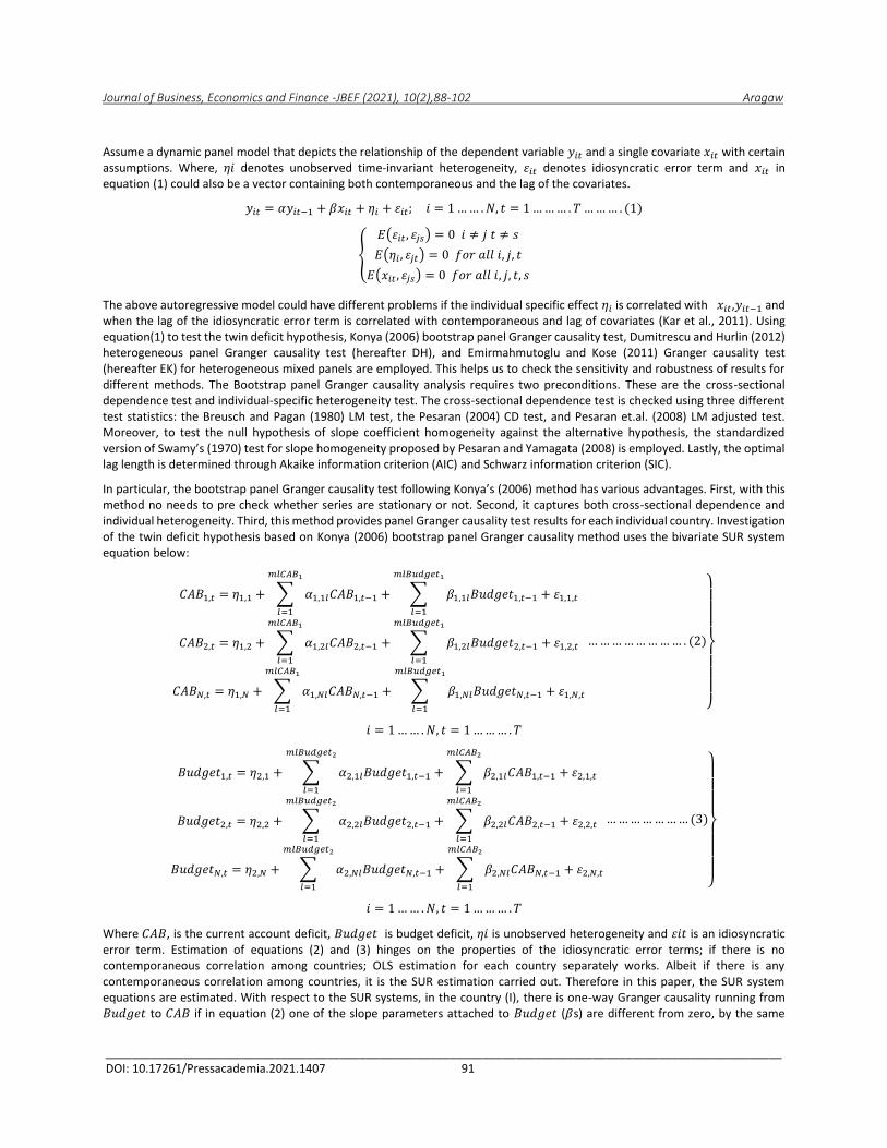
The above autoregressive model could have different problems if the individual specific effect 𝜂𝑖 is correlated with 𝑥𝑖𝑡,𝑦𝑖𝑡−1 and when the lag of the idiosyncratic error term is correlated with contemporaneous and lag of covariates (Kar et al., 2011). Using equation(1) to test the twin deficit hypothesis, Konya (2006) bootstrap panel Granger causality test, Dumitrescu and Hurlin (2012) heterogeneous panel Granger causality test (hereafter DH), and Emirmahmutoglu and Kose (2011) Granger causality test (hereafter EK) for heterogeneous mixed panels are employed. This helps us to check the sensitivity and robustness of results for different methods. The Bootstrap panel Granger causality analysis requires two preconditions. These are the cross-sectional dependence test and individual-specific heterogeneity test. The cross-sectional dependence test is checked using three different test statistics: the Breusch and Pagan (1980) LM test, the Pesaran (2004) CD test, and Pesaran et.al. (2008) LM adjusted test. Moreover, to test the null hypothesis of slope coefficient homogeneity against the alternative hypothesis, the standardized version of Swamy’s (1970) test for slope homogeneity proposed by Pesaran and Yamagata (2008) is employed. Lastly, the optimal lag length is determined through Akaike information criterion (AIC) and Schwarz information criterion (SIC).

In particular, the bootstrap panel Granger causality test following Konya’s (2006) method has various advantages. First, with this method no needs to pre check whether series are stationary or not. Second, it captures both cross-sectional dependence and individual heterogeneity. Third, this method provides panel Granger causality test results for each individual country. Investigation of the twin deficit hypothesis based on Konya (2006) bootstrap panel Granger causality method uses the bivariate SUR system equation below:

𝐶𝐴𝐵1,𝑡 = 𝜂1,1 + ∑ 𝛼1,1𝑙𝐶𝐴𝐵1,𝑡−1

𝑚𝑙𝐶𝐴𝐵1

𝑙=1

+ ∑ 𝛽1,1𝑙𝐵𝑢𝑑𝑔𝑒𝑡1,𝑡−1 + 휀1,1,𝑡

𝑚𝑙𝐵𝑢𝑑𝑔𝑒𝑡1

𝑙=1

𝐶𝐴𝐵2,𝑡 = 𝜂1,2 + ∑ 𝛼1,2𝑙𝐶𝐴𝐵2,𝑡−1


𝑙=1

+ ∑ 𝛽1,2𝑙𝐵𝑢𝑑𝑔𝑒𝑡2,𝑡−1 + 휀1,2,𝑡


𝑙=1

𝐶𝐴𝐵𝑁,𝑡 = 𝜂1,𝑁 + ∑ 𝛼1,𝑁𝑙𝐶𝐴𝐵𝑁,𝑡−1


𝑙=1

+ ∑ 𝛽1,𝑁𝑙𝐵𝑢𝑑𝑔𝑒𝑡𝑁,𝑡−1 + 휀1,𝑁,𝑡


𝑙=1

…………………… . (2)

}

𝑖 = 1…… .𝑁, 𝑡 = 1……… .𝑇

𝐵𝑢𝑑𝑔𝑒𝑡1,𝑡 = 𝜂2,1 + ∑ 𝛼2,1𝑙𝐵𝑢𝑑𝑔𝑒𝑡1,𝑡−1


𝑙=1

+ ∑ 𝛽2,1𝑙𝐶𝐴𝐵1,𝑡−1 + 휀2,1,𝑡


𝑙=1

𝐵𝑢𝑑𝑔𝑒𝑡2,𝑡 = 𝜂2,2 + ∑ 𝛼2,2𝑙𝐵𝑢𝑑𝑔𝑒𝑡2,𝑡−1


𝑙=1

+ ∑ 𝛽2,2𝑙𝐶𝐴𝐵2,𝑡−1 + 휀2,2,𝑡


𝑙=1

𝐵𝑢𝑑𝑔𝑒𝑡𝑁,𝑡 = 𝜂2,𝑁 + ∑ 𝛼2,𝑁𝑙𝐵𝑢𝑑𝑔𝑒𝑡𝑁,𝑡−1


𝑙=1

+ ∑ 𝛽2,𝑁𝑙𝐶𝐴𝐵𝑁,𝑡−1 + 휀2,𝑁,𝑡


𝑙=1

…………………(3)

}

𝑖 = 1…… .𝑁, 𝑡 = 1……… .𝑇

Where 𝐶𝐴𝐵, is the current account deficit, 𝐵𝑢𝑑𝑔𝑒𝑡 is budget deficit, 𝜂𝑖 is unobserved heterogeneity and 휀𝑖𝑡 is an idiosyncratic error term. Estimation of equations (2) and (3) hinges on the properties of the idiosyncratic error terms; if there is no contemporaneous correlation among countries; OLS estimation for each country separately works. Albeit if there is any contemporaneous correlation among countries, it is the SUR estimation carried out. Therefore in this paper, the SUR system equations are estimated. With respect to the SUR systems, in the country (I), there is one-way Granger causality running from 𝐵𝑢𝑑𝑔𝑒𝑡 to 𝐶𝐴𝐵 if in equation (2) one of the slope parameters attached to 𝐵𝑢𝑑𝑔𝑒𝑡 (𝛽s) are different from zero, by the same



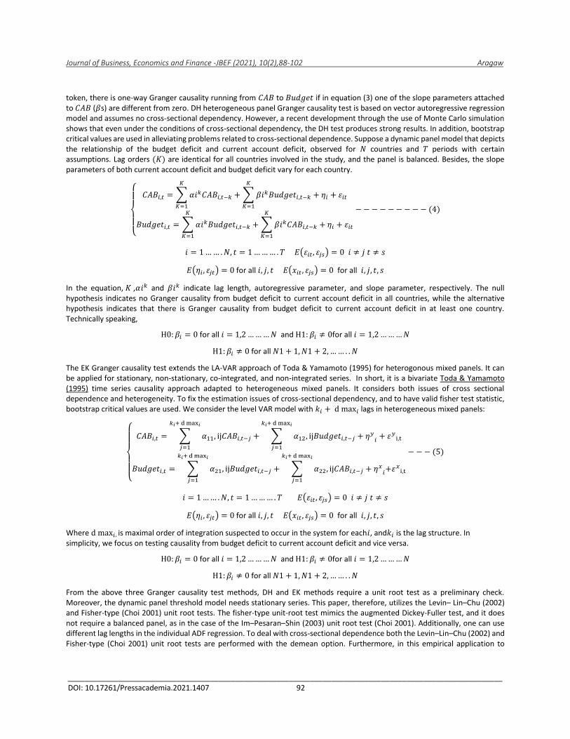
token, there is one-way Granger causality running from 𝐶𝐴𝐵 to 𝐵𝑢𝑑𝑔𝑒𝑡 if in equation (3) one of the slope parameters attached to 𝐶𝐴𝐵 (𝛽s) are different from zero. DH heterogeneous panel Granger causality test is based on vector autoregressive regression model and assumes no cross-sectional dependency. However, a recent development through the use of Monte Carlo simulation shows that even under the conditions of cross-sectional dependency, the DH test produces strong results. In addition, bootstrap critical values are used in alleviating problems related to cross-sectional dependence. Suppose a dynamic panel model that depicts the relationship of the budget deficit and current account deficit, observed for 𝑁 countries and 𝑇 periods with certain assumptions. Lag orders (𝐾) are identical for all countries involved in the study, and the panel is balanced. Besides, the slope parameters of both current account deficit and budget deficit vary for each country.

{

𝐶𝐴𝐵𝑖,𝑡 = ∑ 𝛼𝑖𝑘𝐶𝐴𝐵𝑖,𝑡−𝑘

𝐾

𝐾=1

+∑ 𝛽𝑖𝑘𝐵𝑢𝑑𝑔𝑒𝑡𝑖,𝑡−𝑘

𝐾

𝐾=1

+ 𝜂𝑖 + 휀𝑖𝑡

𝐵𝑢𝑑𝑔𝑒𝑡𝑖,𝑡 = ∑ 𝛼𝑖𝑘𝐵𝑢𝑑𝑔𝑒𝑡𝑖,𝑡−𝑘

𝐾

𝐾=1

+∑ 𝛽𝑖𝑘𝐶𝐴𝐵𝑖,𝑡−𝑘

𝐾

𝐾=1

+ 𝜂𝑖 + 휀𝑖𝑡

− −− − −− − −− (4)

𝑖 = 1…… .𝑁, 𝑡 = 1……… . 𝑇 𝐸(휀𝑖𝑡, 휀𝑗𝑠) = 0 𝑖 ≠ 𝑗 𝑡 ≠ 𝑠

𝐸(𝜂𝑖 , 휀𝑗𝑡) = 0 for all 𝑖, 𝑗, 𝑡 𝐸(𝑥𝑖𝑡 , 휀𝑗𝑠) = 0 for all 𝑖, 𝑗, 𝑡, 𝑠

In the equation, 𝐾 ,𝛼𝑖𝑘 and 𝛽𝑖𝑘 indicate lag length, autoregressive parameter, and slope parameter, respectively. The null hypothesis indicates no Granger causality from budget deficit to current account deficit in all countries, while the alternative hypothesis indicates that there is Granger causality from budget deficit to current account deficit in at least one country. Technically speaking,

H0: 𝛽𝑖 = 0 for all 𝑖 = 1,2………𝑁 and H1: 𝛽𝑖 ≠ 0for all 𝑖 = 1,2………𝑁

H1: 𝛽𝑖 ≠ 0 for all 𝑁1 + 1,𝑁1 + 2,…… . . 𝑁

The EK Granger causality test extends the LA-VAR approach of Toda & Yamamoto (1995) for heterogonous mixed panels. It can be applied for stationary, non-stationary, co-integrated, and non-integrated series. In short, it is a bivariate Toda & Yamamoto (1995) time series causality approach adapted to heterogeneous mixed panels. It considers both issues of cross sectional dependence and heterogeneity. To fix the estimation issues of cross-sectional dependency, and to have valid fisher test statistic, bootstrap critical values are used. We consider the level VAR model with 𝑘𝑖 + d max𝑖 lags in heterogeneous mixed panels:

{

𝐶𝐴𝐵𝑖,𝑡 = ∑ 𝛼11, ij𝐶𝐴𝐵𝑖,𝑡−𝑗

𝑘𝑖+ d max𝑖

𝑗=1

+ ∑ 𝛼12, ij𝐵𝑢𝑑𝑔𝑒𝑡𝑖,𝑡−𝑗

𝑘𝑖+ d max𝑖

𝑗=1

+ 𝜂𝑦𝑖+ 휀𝑦i,t

𝐵𝑢𝑑𝑔𝑒𝑡𝑖,𝑡 = ∑ 𝛼21, ij𝐵𝑢𝑑𝑔𝑒𝑡𝑖,𝑡−𝑗

𝑘𝑖+ d max𝑖

𝑗=1

+ ∑ 𝛼22, ij𝐶𝐴𝐵𝑖,𝑡−𝑗

𝑘𝑖+ d max𝑖

𝑗=1

+ 𝜂𝑥𝑖+휀𝑥i,t

− −− (5)

𝑖 = 1…… .𝑁, 𝑡 = 1……… . 𝑇 𝐸(휀𝑖𝑡, 휀𝑗𝑠) = 0 𝑖 ≠ 𝑗 𝑡 ≠ 𝑠

𝐸(𝜂𝑖 , 휀𝑗𝑡) = 0 for all 𝑖, 𝑗, 𝑡 𝐸(𝑥𝑖𝑡 , 휀𝑗𝑠) = 0 for all 𝑖, 𝑗, 𝑡, 𝑠

Where d max𝑖 , is maximal order of integration suspected to occur in the system for each𝑖, and𝑘𝑖 is the lag structure. In simplicity, we focus on testing causality from budget deficit to current account deficit and vice versa.

H0: 𝛽𝑖 = 0 for all 𝑖 = 1,2………𝑁 and H1: 𝛽𝑖 ≠ 0for all 𝑖 = 1,2………𝑁

H1: 𝛽𝑖 ≠ 0 for all 𝑁1 + 1,𝑁1 + 2,…… . . 𝑁

From the above three Granger causality test methods, DH and EK methods require a unit root test as a preliminary check. Moreover, the dynamic panel threshold model needs stationary series. This paper, therefore, utilizes the Levin– Lin–Chu (2002) and Fisher-type (Choi 2001) unit root tests. The fisher-type unit-root test mimics the augmented Dickey-Fuller test, and it does not require a balanced panel, as in the case of the Im–Pesaran–Shin (2003) unit root test (Choi 2001). Additionally, one can use different lag lengths in the individual ADF regression. To deal with cross-sectional dependence both the Levin–Lin–Chu (2002) and Fisher-type (Choi 2001) unit root tests are performed with the demean option. Furthermore, in this empirical application to



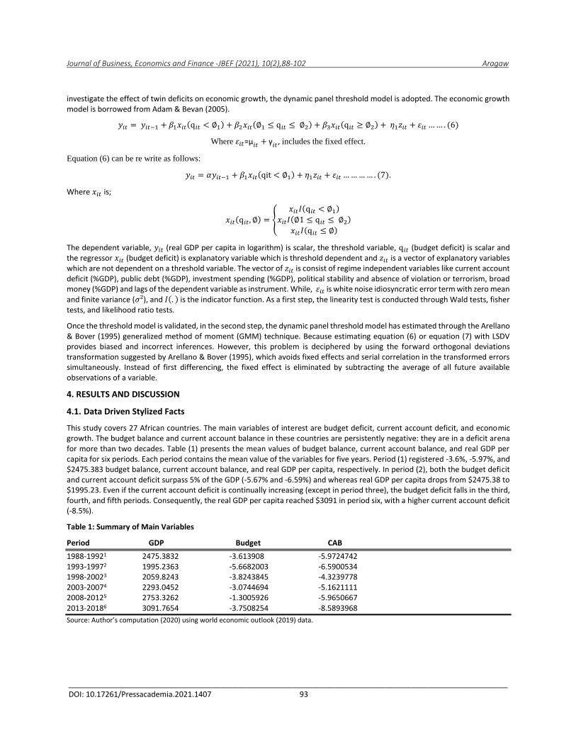
investigate the effect of twin deficits on economic growth, the dynamic panel threshold model is adopted. The economic growth model is borrowed from Adam & Bevan (2005).

𝑦𝑖𝑡 = 𝑦𝑖𝑡−1 + 𝛽1𝑥𝑖𝑡(q𝑖𝑡 < ∅1) + 𝛽2𝑥𝑖𝑡(∅1 ≤ q𝑖𝑡 ≤ ∅2) + 𝛽3𝑥𝑖𝑡(q𝑖𝑡 ≥ ∅2) + 𝜂1𝑧𝑖𝑡 + 휀𝑖𝑡 …… . (6)

Where 휀𝑖𝑡=µ𝑖𝑡 + γ𝑖𝑡, includes the fixed effect.

Equation (6) can be re write as follows:

𝑦𝑖𝑡 = 𝛼𝑦𝑖𝑡−1 + 𝛽1𝑥𝑖𝑡(qit < ∅1) + 𝜂1𝑧𝑖𝑡 + 휀𝑖𝑡 ………… . (7).

Where 𝑥𝑖𝑡 is;

𝑥𝑖𝑡(q𝑖𝑡, ∅) = {

𝑥𝑖𝑡𝐼(q𝑖𝑡 < ∅1)

𝑥𝑖𝑡𝐼(∅1 ≤ q𝑖𝑡 ≤ ∅2)

𝑥𝑖𝑡𝐼(q𝑖𝑡 ≤ ∅)

The dependent variable, 𝑦𝑖𝑡 (real GDP per capita in logarithm) is scalar, the threshold variable, q𝑖𝑡 (budget deficit) is scalar and the regressor 𝑥𝑖𝑡 (budget deficit) is explanatory variable which is threshold dependent and 𝑧𝑖𝑡 is a vector of explanatory variables which are not dependent on a threshold variable. The vector of 𝑧𝑖𝑡 is consist of regime independent variables like current account deficit (%GDP), public debt (%GDP), investment spending (%GDP), political stability and absence of violation or terrorism, broad money (%GDP) and lags of the dependent variable as instrument. While, 휀𝑖𝑡 is white noise idiosyncratic error term with zero mean and finite variance (𝜎²), and 𝐼(. ) is the indicator function. As a first step, the linearity test is conducted through Wald tests, fisher tests, and likelihood ratio tests.

Once the threshold model is validated, in the second step, the dynamic panel threshold model has estimated through the Arellano & Bover (1995) generalized method of moment (GMM) technique. Because estimating equation (6) or equation (7) with LSDV provides biased and incorrect inferences. However, this problem is deciphered by using the forward orthogonal deviations transformation suggested by Arellano & Bover (1995), which avoids fixed effects and serial correlation in the transformed errors simultaneously. Instead of first differencing, the fixed effect is eliminated by subtracting the average of all future available observations of a variable.

4. RESULTS AND DISCUSSION

4.1. Data Driven Stylized Facts

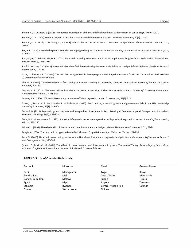
This study covers 27 African countries. The main variables of interest are budget deficit, current account deficit, and economic growth. The budget balance and current account balance in these countries are persistently negative: they are in a deficit arena for more than two decades. Table (1) presents the mean values of budget balance, current account balance, and real GDP per capita for six periods. Each period contains the mean value of the variables for five years. Period (1) registered -3.6%, -5.97%, and $2475.383 budget balance, current account balance, and real GDP per capita, respectively. In period (2), both the budget deficit and current account deficit surpass 5% of the GDP (-5.67% and -6.59%) and whereas real GDP per capita drops from $2475.38 to $1995.23. Even if the current account deficit is continually increasing (except in period three), the budget deficit falls in the third, fourth, and fifth periods. Consequently, the real GDP per capita reached $3091 in period six, with a higher current account deficit (-8.5%).

Table 1: Summary of Main Variables

Period GDP Budget CAB

1988-19921 2475.3832 -3.613908 -5.9724742 1993-19972 1995.2363 -5.6682003 -6.5900534 1998-20023 2059.8243 -3.8243845 -4.3239778

2003-20074 2293.0452 -3.0744694 -5.1621111 2008-20125 2753.3262 -1.3005926 -5.9650667 2013-20186 3091.7654 -3.7508254 -8.5893968

Source: Author’s computation (2020) using world economic outlook (2019) data.



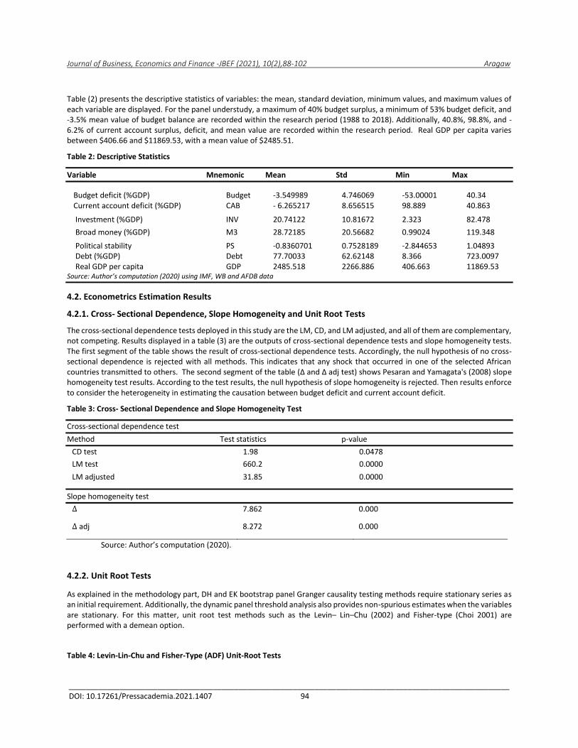
Table (2) presents the descriptive statistics of variables: the mean, standard deviation, minimum values, and maximum values of each variable are displayed. For the panel understudy, a maximum of 40% budget surplus, a minimum of 53% budget deficit, and -3.5% mean value of budget balance are recorded within the research period (1988 to 2018). Additionally, 40.8%, 98.8%, and - 6.2% of current account surplus, deficit, and mean value are recorded within the research period. Real GDP per capita varies between $406.66 and $11869.53, with a mean value of $2485.51.

Table 2: Descriptive Statistics

Variable Mnemonic Mean Std Min Max

Budget deficit (%GDP) Budget -3.549989 4.746069 -53.00001 40.34 Current account deficit (%GDP) CAB - 6.265217 8.656515 98.889 40.863

Investment (%GDP) INV 20.74122 10.81672 2.323 82.478

Broad money (%GDP) M3 28.72185 20.56682 0.99024 119.348

Political stability PS -0.8360701 0.7528189 -2.844653 1.04893 Debt (%GDP) Debt 77.70033 62.62148 8.366 723.0097 Real GDP per capita GDP 2485.518 2266.886 406.663 11869.53 Source: Author’s computation (2020) using IMF, WB and AFDB data

4.2. Econometrics Estimation Results

4.2.1. Cross- Sectional Dependence, Slope Homogeneity and Unit Root Tests

The cross-sectional dependence tests deployed in this study are the LM, CD, and LM adjusted, and all of them are complementary, not competing. Results displayed in a table (3) are the outputs of cross-sectional dependence tests and slope homogeneity tests. The first segment of the table shows the result of cross-sectional dependence tests. Accordingly, the null hypothesis of no cross-sectional dependence is rejected with all methods. This indicates that any shock that occurred in one of the selected African countries transmitted to others. The second segment of the table (∆ and ∆ adj test) shows Pesaran and Yamagata's (2008) slope homogeneity test results. According to the test results, the null hypothesis of slope homogeneity is rejected. Then results enforce to consider the heterogeneity in estimating the causation between budget deficit and current account deficit.

Table 3: Cross- Sectional Dependence and Slope Homogeneity Test

Cross-sectional dependence test

Method Test statistics p-value

CD test 1.98 0.0478

LM test 660.2 0.0000

LM adjusted 31.85 0.0000

Slope homogeneity test

∆ 7.862 0.000

∆ adj 8.272 0.000

Source: Author’s computation (2020).

4.2.2. Unit Root Tests

As explained in the methodology part, DH and EK bootstrap panel Granger causality testing methods require stationary series as an initial requirement. Additionally, the dynamic panel threshold analysis also provides non-spurious estimates when the variables are stationary. For this matter, unit root test methods such as the Levin– Lin–Chu (2002) and Fisher-type (Choi 2001) are performed with a demean option.

Table 4: Levin-Lin-Chu and Fisher-Type (ADF) Unit-Root Tests



Variables Levin-Lin-Chu unit-root test Fisher type (ADF) unit-root test

Budget -6.6174*** 24.0555***

CAB -6.7817*** 21.1601***

INV -5.4134 *** 14.8397***

M3 -1.9114** 12.4113***

PS 0.2047 9.2571***

Debt -4.7997*** 13.0194***

GDP -1.8563 ** 11.0212***

*** p<0.01, ** p<0.05, * p<0.1 Source: Author’s computation (2020).

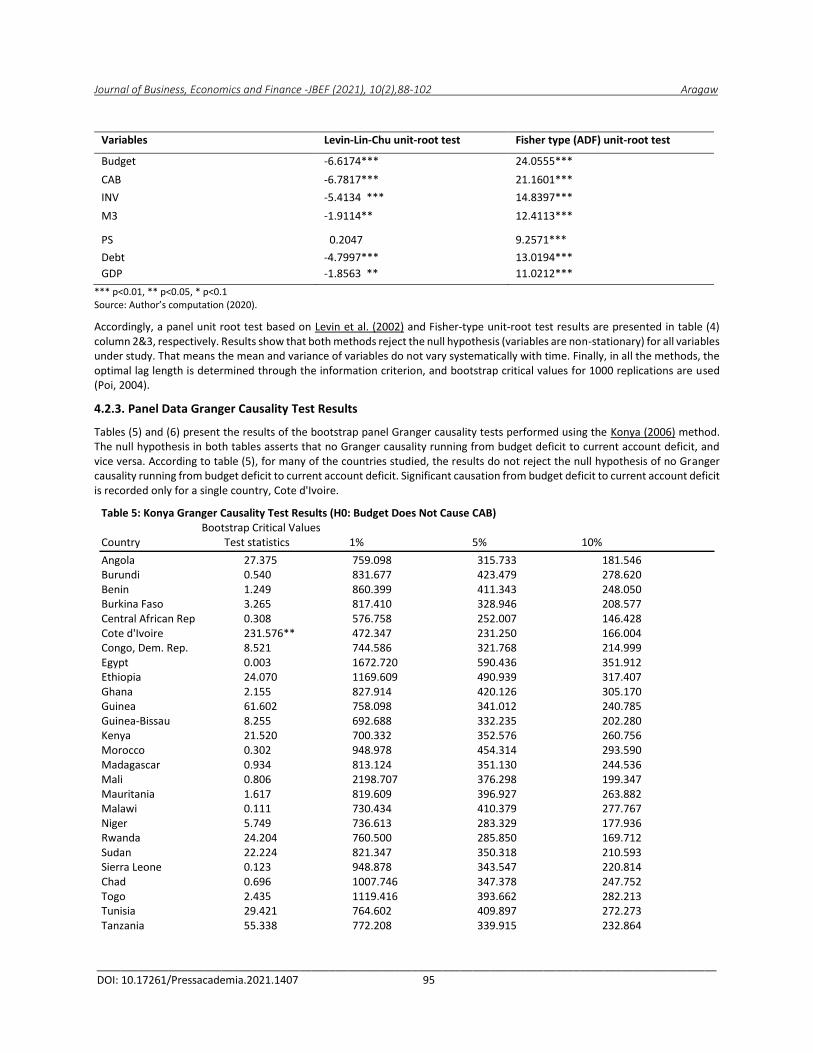
Accordingly, a panel unit root test based on Levin et al. (2002) and Fisher-type unit-root test results are presented in table (4) column 2&3, respectively. Results show that both methods reject the null hypothesis (variables are non-stationary) for all variables under study. That means the mean and variance of variables do not vary systematically with time. Finally, in all the methods, the optimal lag length is determined through the information criterion, and bootstrap critical values for 1000 replications are used (Poi, 2004).

4.2.3. Panel Data Granger Causality Test Results

Tables (5) and (6) present the results of the bootstrap panel Granger causality tests performed using the Konya (2006) method. The null hypothesis in both tables asserts that no Granger causality running from budget deficit to current account deficit, and vice versa. According to table (5), for many of the countries studied, the results do not reject the null hypothesis of no Granger causality running from budget deficit to current account deficit. Significant causation from budget deficit to current account deficit is recorded only for a single country, Cote d'Ivoire.

Table 5: Konya Granger Causality Test Results (H0: Budget Does Not Cause CAB) Bootstrap Critical Values Country Test statistics 1% 5% 10%

Angola 27.375 759.098 315.733 181.546 Burundi 0.540 831.677 423.479 278.620 Benin 1.249 860.399 411.343 248.050 Burkina Faso 3.265 817.410 328.946 208.577 Central African Rep 0.308 576.758 252.007 146.428 Cote d'Ivoire 231.576** 472.347 231.250 166.004 Congo, Dem. Rep. 8.521 744.586 321.768 214.999 Egypt 0.003 1672.720 590.436 351.912 Ethiopia 24.070 1169.609 490.939 317.407 Ghana 2.155 827.914 420.126 305.170 Guinea 61.602 758.098 341.012 240.785 Guinea-Bissau 8.255 692.688 332.235 202.280 Kenya 21.520 700.332 352.576 260.756 Morocco 0.302 948.978 454.314 293.590 Madagascar 0.934 813.124 351.130 244.536 Mali 0.806 2198.707 376.298 199.347 Mauritania 1.617 819.609 396.927 263.882 Malawi 0.111 730.434 410.379 277.767 Niger 5.749 736.613 283.329 177.936 Rwanda 24.204 760.500 285.850 169.712 Sudan 22.224 821.347 350.318 210.593 Sierra Leone 0.123 948.878 343.547 220.814 Chad 0.696 1007.746 347.378 247.752 Togo 2.435 1119.416 393.662 282.213 Tunisia 29.421 764.602 409.897 272.273 Tanzania 55.338 772.208 339.915 232.864



Uganda 34.951 535.263 279.172 181.205 Source: Author’s computation (2020) using GAUSS 20. Note: *** p<0.01, ** p<0.05, * p<0.1.

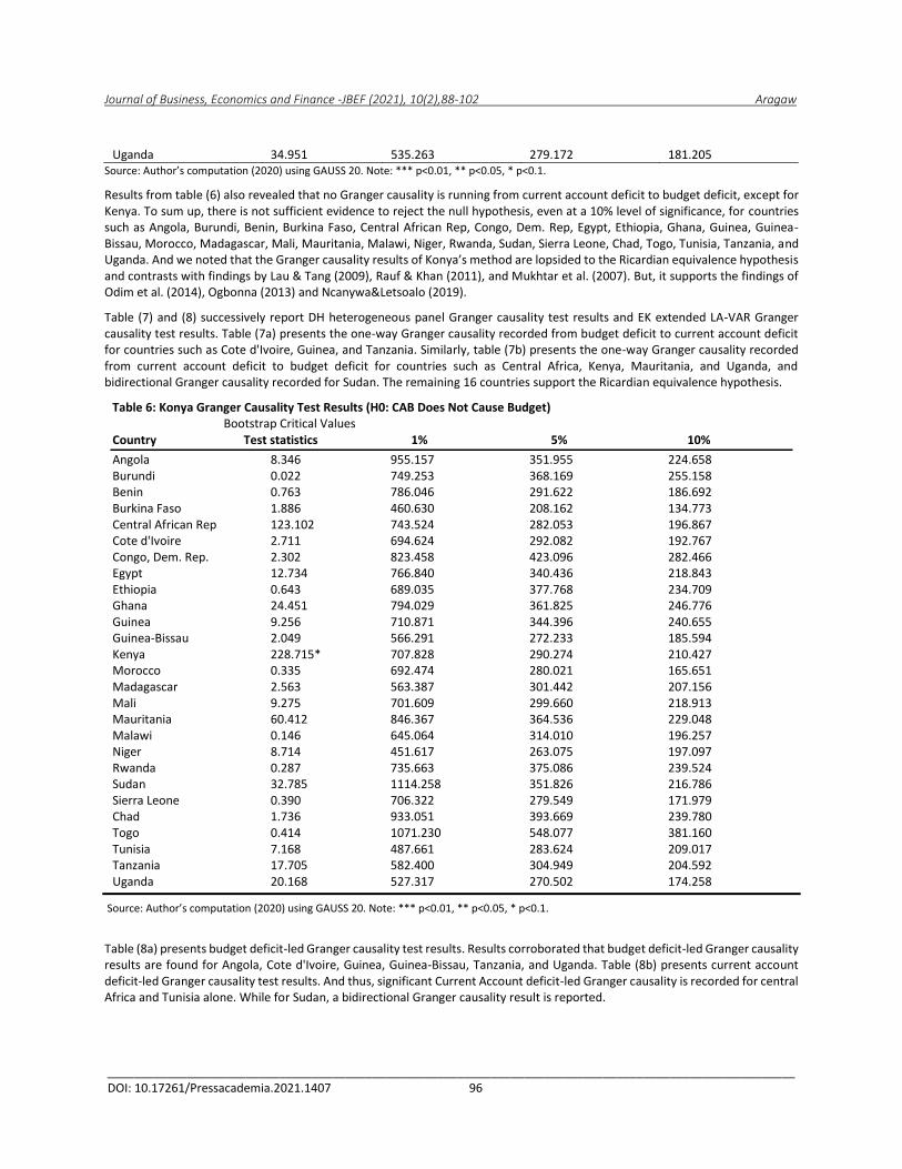
Results from table (6) also revealed that no Granger causality is running from current account deficit to budget deficit, except for Kenya. To sum up, there is not sufficient evidence to reject the null hypothesis, even at a 10% level of significance, for countries such as Angola, Burundi, Benin, Burkina Faso, Central African Rep, Congo, Dem. Rep, Egypt, Ethiopia, Ghana, Guinea, Guinea-Bissau, Morocco, Madagascar, Mali, Mauritania, Malawi, Niger, Rwanda, Sudan, Sierra Leone, Chad, Togo, Tunisia, Tanzania, and Uganda. And we noted that the Granger causality results of Konya’s method are lopsided to the Ricardian equivalence hypothesis and contrasts with findings by Lau & Tang (2009), Rauf & Khan (2011), and Mukhtar et al. (2007). But, it supports the findings of Odim et al. (2014), Ogbonna (2013) and Ncanywa&Letsoalo (2019).

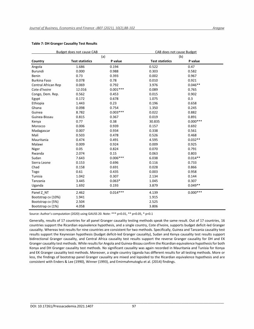
Table (7) and (8) successively report DH heterogeneous panel Granger causality test results and EK extended LA-VAR Granger causality test results. Table (7a) presents the one-way Granger causality recorded from budget deficit to current account deficit for countries such as Cote d'Ivoire, Guinea, and Tanzania. Similarly, table (7b) presents the one-way Granger causality recorded from current account deficit to budget deficit for countries such as Central Africa, Kenya, Mauritania, and Uganda, and bidirectional Granger causality recorded for Sudan. The remaining 16 countries support the Ricardian equivalence hypothesis.

Table 6: Konya Granger Causality Test Results (H0: CAB Does Not Cause Budget) Bootstrap Critical Values Country Test statistics 1% 5% 10%

Angola 8.346 955.157 351.955 224.658 Burundi 0.022 749.253 368.169 255.158 Benin 0.763 786.046 291.622 186.692 Burkina Faso 1.886 460.630 208.162 134.773 Central African Rep 123.102 743.524 282.053 196.867 Cote d'Ivoire 2.711 694.624 292.082 192.767 Congo, Dem. Rep. 2.302 823.458 423.096 282.466 Egypt 12.734 766.840 340.436 218.843 Ethiopia 0.643 689.035 377.768 234.709 Ghana 24.451 794.029 361.825 246.776 Guinea 9.256 710.871 344.396 240.655 Guinea-Bissau 2.049 566.291 272.233 185.594 Kenya 228.715* 707.828 290.274 210.427 Morocco 0.335 692.474 280.021 165.651 Madagascar 2.563 563.387 301.442 207.156 Mali 9.275 701.609 299.660 218.913 Mauritania 60.412 846.367 364.536 229.048 Malawi 0.146 645.064 314.010 196.257 Niger 8.714 451.617 263.075 197.097 Rwanda 0.287 735.663 375.086 239.524 Sudan 32.785 1114.258 351.826 216.786 Sierra Leone 0.390 706.322 279.549 171.979 Chad 1.736 933.051 393.669 239.780 Togo 0.414 1071.230 548.077 381.160 Tunisia 7.168 487.661 283.624 209.017 Tanzania 17.705 582.400 304.949 204.592 Uganda 20.168 527.317 270.502 174.258

Source: Author’s computation (2020) using GAUSS 20. Note: *** p<0.01, ** p<0.05, * p<0.1.

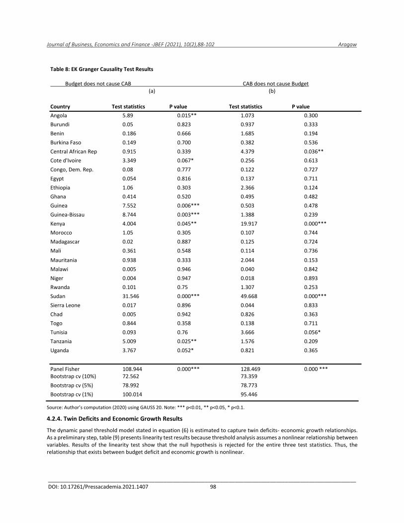
Table (8a) presents budget deficit-led Granger causality test results. Results corroborated that budget deficit-led Granger causality results are found for Angola, Cote d'Ivoire, Guinea, Guinea-Bissau, Tanzania, and Uganda. Table (8b) presents current account deficit-led Granger causality test results. And thus, significant Current Account deficit-led Granger causality is recorded for central Africa and Tunisia alone. While for Sudan, a bidirectional Granger causality result is reported.



Table 7: DH Granger Causality Test Results

Budget does not cause CAB CAB does not cause Budget (a) (b)

Country Test statistics P value Test statistics P value

Angola 1.686 0.194 0.522 0.47 Burundi 0.000 0.988 0.303 0.582 Benin 0.73 0.393 0.002 0.967 Burkina Faso 0.078 0.78 0.010 0.921 Central African Rep 0.069 0.792 3.976 0.046** Cote d'Ivoire 12.016 0.001*** 0.089 0.765 Congo, Dem. Rep. 0.562 0.453 0.015 0.902 Egypt 0.172 0.678 1.075 0.3 Ethiopia 1.443 0.23 0.196 0.658 Ghana 0.098 0.754 1.350 0.245 Guinea 8.782 0.003*** 0.022 0.882 Guinea-Bissau 0.815 0.367 0.019 0.891 Kenya 0.77 0.38 30.835 0.000*** Morocco 0.006 0.939 0.157 0.692 Madagascar 0.007 0.934 0.338 0.561 Mali 0.503 0.478 0.526 0.468 Mauritania 0.474 0.491 4.595 0.032** Malawi 0.009 0.924 0.009 0.925 Niger 0.05 0.824 0.070 0.791 Rwanda 2.074 0.15 0.063 0.803 Sudan 7.643 0.006*** 6.038 0.014** Sierra Leone 0.153 0.696 0.116 0.733 Chad 0.158 0.691 0.028 0.866 Togo 0.61 0.435 0.003 0.958 Tunisia 1.042 0.307 2.134 0.144 Tanzania 3.445 0.063* 1.045 0.307 Uganda 1.692 0.193 3.879 0.049**

Panel Z_NT 2.462 0.014*** 4.139 0.000*** Bootstrap cv (10%) 1.941 1.915 Bootstrap cv (5%) 2.504 2.525 Bootstrap cv (1%) 4.058 3.806

Source: Author’s computation (2020) using GAUSS 20. Note: *** p<0.01, ** p<0.05, * p<0.1

Generally, results of 17 countries for all panel Granger causality testing methods speak the same result. Out of 17 countries, 16 countries support the Ricardian equivalence hypothesis, and a single country, Cote d'Ivoire, supports budget deficit-led Granger causality. Whereas test results for nine countries are consistent for two methods. Specifically, Guinea and Tanzania causality test results support the Keynesian hypothesis (budget deficit-led Granger causality), Sudan and Kenya causality test results support bidirectional Granger causality, and Central Africa causality test results support the reverse Granger causality for DH and EK Granger causality test methods. While results for Angola and Guinea-Bissau confirm the Ricardian equivalence hypothesis for both Konya and DH Granger causality test methods. No significant causality was again recorded in Mauritania and Tunisia for Konya and EK Granger causality test methods. Moreover, a single country Uganda has different results for all testing methods. More or less, the findings of bootstrap panel Granger causality are mixed and lopsided to the Ricardian equivalence hypothesis and are consistent with Enders & Lee (1990), Winner (1993), and Emirmahmutoglu et al. (2014) findings.



Table 8: EK Granger Causality Test Results Budget does not cause CAB CAB does not cause Budget

(a) (b)

Country Test statistics P value Test statistics P value

Angola 5.89 0.015** 1.073 0.300

Burundi 0.05 0.823 0.937 0.333

Benin 0.186 0.666 1.685 0.194

Burkina Faso 0.149 0.700 0.382 0.536

Central African Rep 0.915 0.339 4.379 0.036**

Cote d'Ivoire 3.349 0.067* 0.256 0.613

Congo, Dem. Rep. 0.08 0.777 0.122 0.727

Egypt 0.054 0.816 0.137 0.711

Ethiopia 1.06 0.303 2.366 0.124

Ghana 0.414 0.520 0.495 0.482

Guinea 7.552 0.006*** 0.503 0.478

Guinea-Bissau 8.744 0.003*** 1.388 0.239

Kenya 4.004 0.045** 19.917 0.000***

Morocco 1.05 0.305 0.107 0.744

Madagascar 0.02 0.887 0.125 0.724

Mali 0.361 0.548 0.114 0.736

Mauritania 0.938 0.333 2.044 0.153

Malawi 0.005 0.946 0.040 0.842

Niger 0.004 0.947 0.018 0.893

Rwanda 0.101 0.75 1.307 0.253

Sudan 31.546 0.000*** 49.668 0.000***

Sierra Leone 0.017 0.896 0.044 0.833

Chad 0.005 0.942 0.826 0.363

Togo 0.844 0.358 0.138 0.711

Tunisia 0.093 0.76 3.666 0.056*

Tanzania 5.009 0.025** 1.576 0.209

Uganda 3.767 0.052* 0.821 0.365

Panel Fisher 108.944 0.000*** 128.469 0.000 *** Bootstrap cv (10%) 72.562 73.359

Bootstrap cv (5%) 78.992 78.773

Bootstrap cv (1%) 100.014 95.446

Source: Author’s computation (2020) using GAUSS 20. Note: *** p<0.01, ** p<0.05, * p<0.1.

4.2.4. Twin Deficits and Economic Growth Results

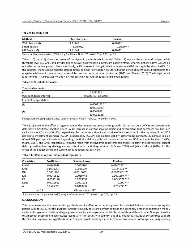
The dynamic panel threshold model stated in equation (6) is estimated to capture twin deficits- economic growth relationships. As a preliminary step, table (9) presents linearity test results because threshold analysis assumes a nonlinear relationship between variables. Results of the linearity test show that the null hypothesis is rejected for the entire three test statistics. Thus, the relationship that exists between budget deficit and economic growth is nonlinear.



Table 9: Linearity Test

Method Test statistics p-value

Wald Tests (LM) 12.81245 0.0768* Fisher Tests (F) 1370.932 0.0000*** LRT Tests (LM) 12.91844 0.0741*

Source: Authors computation (2020) using R software. Note: *** p<0.01, ** p<0.05, * p<0.1

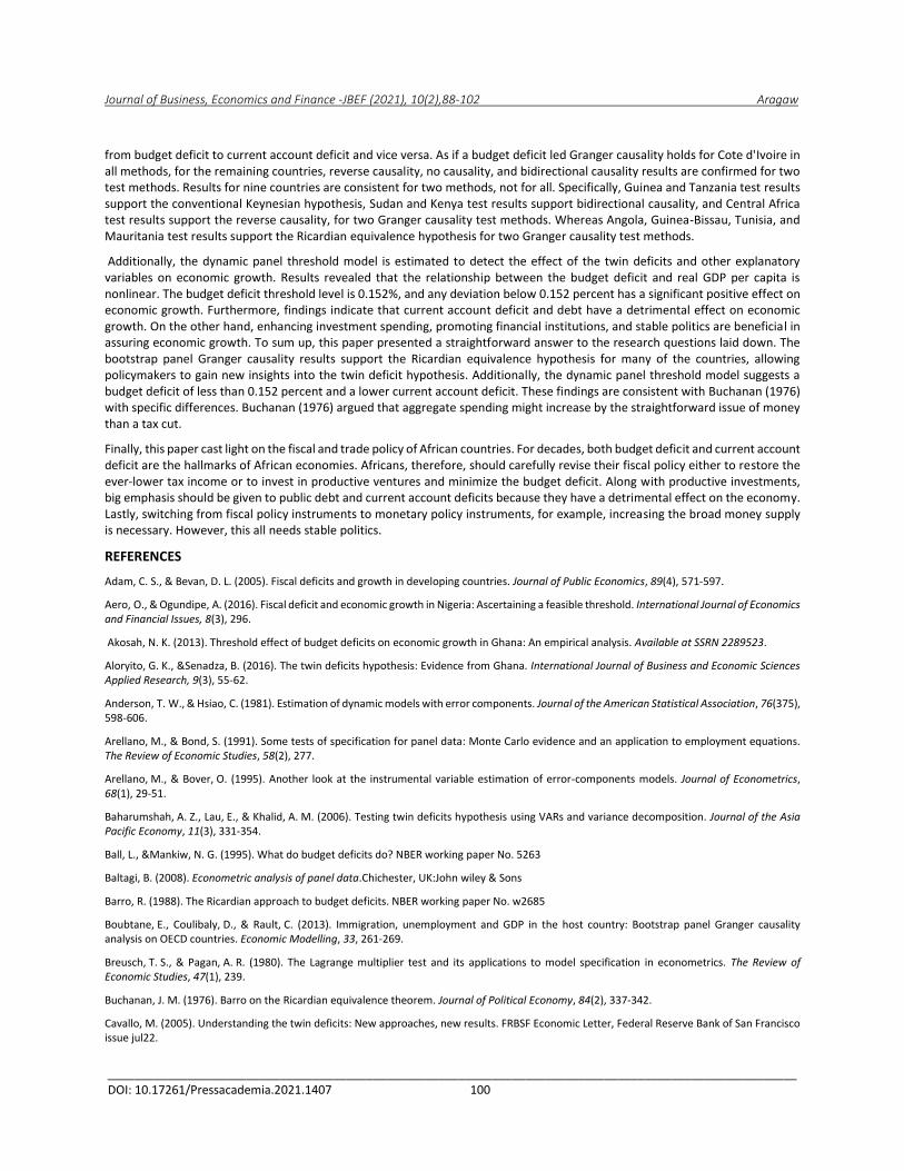
Tables (10) and (11) show the results of the dynamic panel threshold model. Table (11) reports the estimated budget deficit threshold level (0.152%), and any deviations below this level have a significant positive effect, whereas deficits above 0.152% do not affect economic growth. More specifically, a 1% increase in budget deficit increases real GDP per capita by about 0.62%. On the contrary, the result nullified the budget deficit- real GDP per capita nexus for a budget deficit above 0.152%. Even though the magnitude is lower, in comparison, our result is consistent with the results of Akosah (2013) and Slimani (2016). The budget deficit is detrimental if it surpasses 4% and 4.8%, respectively, for Akosah (2013) and Slimani (2016).

Table 10: Threshold Estimates

Threshold estimates

γ 0.1522852 95% confidence interval (0.0000761, 1.55893)

Effect of budget deficit

𝛽1 0.0062165 ** (0.0030005) 𝛽2 0.0049876 (0.0033088)

Source: Author’s computation (2020) using R software. Note: *** p<0.01, ** p<0.05, * p<0.1

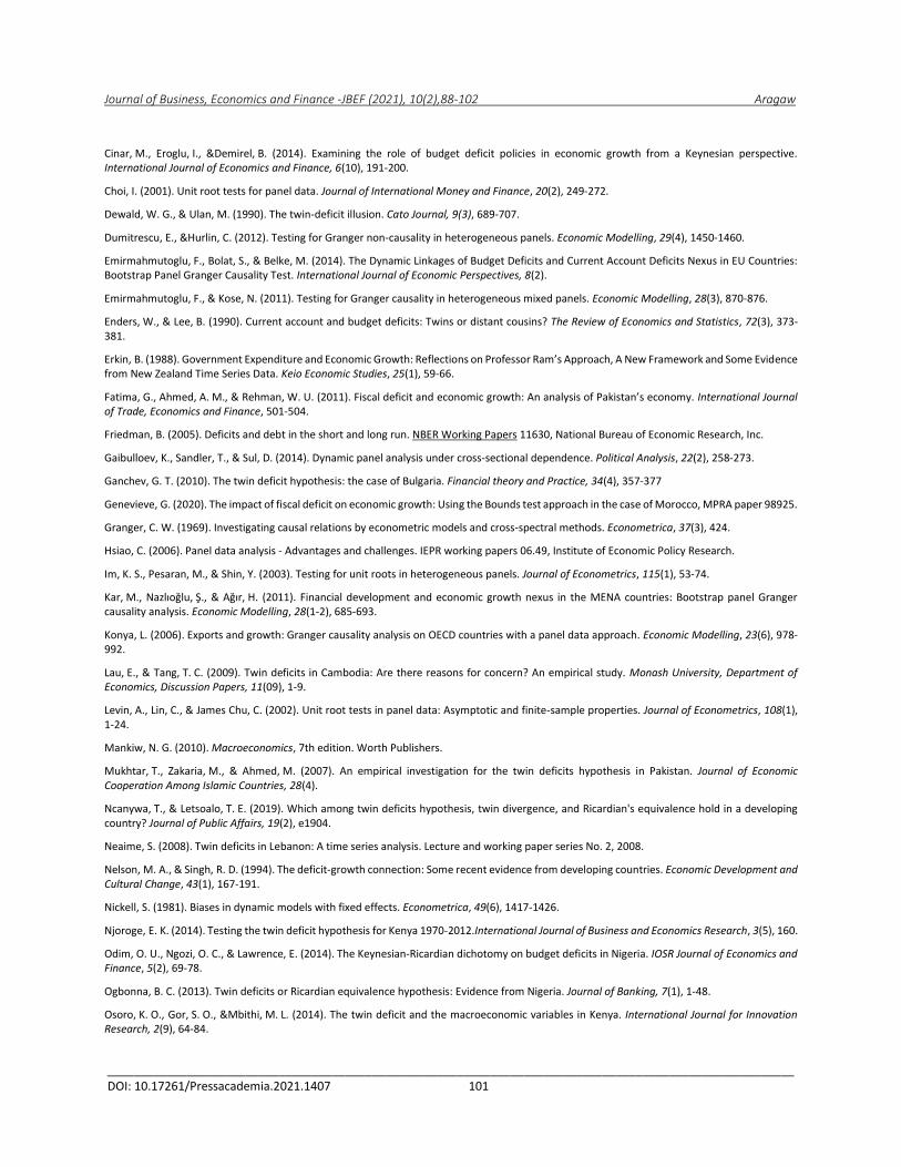
Table (11) presents the effect of regime-independent regressors on economic growth. Current account deficits and government debt have a significant negative effect. A 1% increase in current account deficit and government debt decreases real GDP per capita by about 0.4% and 0.17%, respectively. Furthermore, a significant positive effect is reported for the lag value of real GDP per capita, investment spending (%GDP), broad money (%GDP), and political stability. Other things constant, 1% increase in a lag of real GDP per capita, investment spending, political stability, and broad money increases real GDP per capita by about 1.47%, 0.51%, 0.56%, and 0.4%, respectively. Thus, the result from the dynamic panel threshold model is against the conventional budget deficit growth-enhancing strategy and consistent with the findings of Adam & Bevan (2005) and Şahin & Mucuk (2014), for the effect of the budget deficit and current account deficit, respectively.

Table 11: Effect of regime independent regressors

Covariates Coefficients Standard error P-value

Initial 0.0147048 0.0065160 0.0240257 ** CAB -0.0039256 0.0018559 0.0344163 ** INV 0.0051700 0.0013685 0.0001582 *** M3 0.0040562 0.0010748 0.0001607 *** PS 0.0593146 0.0209092 0.0045572 *** Debt -0.0016962 0.0001938 0.000 *** 𝛿 0.0525698 0.0189732 0.005593 **

N= 27 Observations= 837

Source: Authors computation (2020) using R software. Note: *** p<0.01, ** p<0.05, * p<0.1

5. CONCLUSION

This paper examines the twin deficit hypothesis and its effect on economic growth for selected African countries covering the period 1988 to 2018. For this purpose, Granger causality tests are performed using the seemingly unrelated regression model, vector autoregressive model, and lag augmented vector autoregressive model. Results of three different panel Granger causality test methods presented mixed results; results vary from country to country, out of 27 countries, results of 16 countries support the Ricardian equivalence hypothesis for all Granger causality testing methods. That means there is no Granger causality running



from budget deficit to current account deficit and vice versa. As if a budget deficit led Granger causality holds for Cote d'Ivoire in all methods, for the remaining countries, reverse causality, no causality, and bidirectional causality results are confirmed for two test methods. Results for nine countries are consistent for two methods, not for all. Specifically, Guinea and Tanzania test results support the conventional Keynesian hypothesis, Sudan and Kenya test results support bidirectional causality, and Central Africa test results support the reverse causality, for two Granger causality test methods. Whereas Angola, Guinea-Bissau, Tunisia, and Mauritania test results support the Ricardian equivalence hypothesis for two Granger causality test methods.

Additionally, the dynamic panel threshold model is estimated to detect the effect of the twin deficits and other explanatory variables on economic growth. Results revealed that the relationship between the budget deficit and real GDP per capita is nonlinear. The budget deficit threshold level is 0.152%, and any deviation below 0.152 percent has a significant positive effect on economic growth. Furthermore, findings indicate that current account deficit and debt have a detrimental effect on economic growth. On the other hand, enhancing investment spending, promoting financial institutions, and stable politics are beneficial in assuring economic growth. To sum up, this paper presented a straightforward answer to the research questions laid down. The bootstrap panel Granger causality results support the Ricardian equivalence hypothesis for many of the countries, allowing policymakers to gain new insights into the twin deficit hypothesis. Additionally, the dynamic panel threshold model suggests a budget deficit of less than 0.152 percent and a lower current account deficit. These findings are consistent with Buchanan (1976) with specific differences. Buchanan (1976) argued that aggregate spending might increase by the straightforward issue of money than a tax cut.

Finally, this paper cast light on the fiscal and trade policy of African countries. For decades, both budget deficit and current account deficit are the hallmarks of African economies. Africans, therefore, should carefully revise their fiscal policy either to restore the ever-lower tax income or to invest in productive ventures and minimize the budget deficit. Along with productive investments, big emphasis should be given to public debt and current account deficits because they have a detrimental effect on the economy. Lastly, switching from fiscal policy instruments to monetary policy instruments, for example, increasing the broad money supply is necessary. However, this all needs stable politics.

REFERENCES

Adam, C. S., & Bevan, D. L. (2005). Fiscal deficits and growth in developing countries. Journal of Public Economics, 89(4), 571-597.

Aero, O., & Ogundipe, A. (2016). Fiscal deficit and economic growth in Nigeria: Ascertaining a feasible threshold. International Journal of Economics and Financial Issues, 8(3), 296.

Akosah, N. K. (2013). Threshold effect of budget deficits on economic growth in Ghana: An empirical analysis. Available at SSRN 2289523.

Aloryito, G. K., &Senadza, B. (2016). The twin deficits hypothesis: Evidence from Ghana. International Journal of Business and Economic Sciences Applied Research, 9(3), 55-62.

Anderson, T. W., & Hsiao, C. (1981). Estimation of dynamic models with error components. Journal of the American Statistical Association, 76(375), 598-606.

Arellano, M., & Bond, S. (1991). Some tests of specification for panel data: Monte Carlo evidence and an application to employment equations. The Review of Economic Studies, 58(2), 277.

Arellano, M., & Bover, O. (1995). Another look at the instrumental variable estimation of error-components models. Journal of Econometrics, 68(1), 29-51.

Baharumshah, A. Z., Lau, E., & Khalid, A. M. (2006). Testing twin deficits hypothesis using VARs and variance decomposition. Journal of the Asia Pacific Economy, 11(3), 331-354.

Ball, L., &Mankiw, N. G. (1995). What do budget deficits do? NBER working paper No. 5263

Baltagi, B. (2008). Econometric analysis of panel data.Chichester, UK:John wiley & Sons

Barro, R. (1988). The Ricardian approach to budget deficits. NBER working paper No. w2685

Boubtane, E., Coulibaly, D., & Rault, C. (2013). Immigration, unemployment and GDP in the host country: Bootstrap panel Granger causality analysis on OECD countries. Economic Modelling, 33, 261-269.

Breusch, T. S., & Pagan, A. R. (1980). The Lagrange multiplier test and its applications to model specification in econometrics. The Review of Economic Studies, 47(1), 239.

Buchanan, J. M. (1976). Barro on the Ricardian equivalence theorem. Journal of Political Economy, 84(2), 337-342.

Cavallo, M. (2005). Understanding the twin deficits: New approaches, new results. FRBSF Economic Letter, Federal Reserve Bank of San Francisco issue jul22.



Cinar, M., Eroglu, I., &Demirel, B. (2014). Examining the role of budget deficit policies in economic growth from a Keynesian perspective. International Journal of Economics and Finance, 6(10), 191-200.

Choi, I. (2001). Unit root tests for panel data. Journal of International Money and Finance, 20(2), 249-272.

Dewald, W. G., & Ulan, M. (1990). The twin-deficit illusion. Cato Journal, 9(3), 689-707.

Dumitrescu, E., &Hurlin, C. (2012). Testing for Granger non-causality in heterogeneous panels. Economic Modelling, 29(4), 1450-1460.

Emirmahmutoglu, F., Bolat, S., & Belke, M. (2014). The Dynamic Linkages of Budget Deficits and Current Account Deficits Nexus in EU Countries: Bootstrap Panel Granger Causality Test. International Journal of Economic Perspectives, 8(2).

Emirmahmutoglu, F., & Kose, N. (2011). Testing for Granger causality in heterogeneous mixed panels. Economic Modelling, 28(3), 870-876.

Enders, W., & Lee, B. (1990). Current account and budget deficits: Twins or distant cousins? The Review of Economics and Statistics, 72(3), 373-381.

Erkin, B. (1988). Government Expenditure and Economic Growth: Reflections on Professor Ram’s Approach, A New Framework and Some Evidence from New Zealand Time Series Data. Keio Economic Studies, 25(1), 59-66.

Fatima, G., Ahmed, A. M., & Rehman, W. U. (2011). Fiscal deficit and economic growth: An analysis of Pakistan’s economy. International Journal of Trade, Economics and Finance, 501-504.

Friedman, B. (2005). Deficits and debt in the short and long run. NBER Working Papers 11630, National Bureau of Economic Research, Inc.

Gaibulloev, K., Sandler, T., & Sul, D. (2014). Dynamic panel analysis under cross-sectional dependence. Political Analysis, 22(2), 258-273.

Ganchev, G. T. (2010). The twin deficit hypothesis: the case of Bulgaria. Financial theory and Practice, 34(4), 357-377

Genevieve, G. (2020). The impact of fiscal deficit on economic growth: Using the Bounds test approach in the case of Morocco, MPRA paper 98925.

Granger, C. W. (1969). Investigating causal relations by econometric models and cross-spectral methods. Econometrica, 37(3), 424.

Hsiao, C. (2006). Panel data analysis - Advantages and challenges. IEPR working papers 06.49, Institute of Economic Policy Research.

Im, K. S., Pesaran, M., & Shin, Y. (2003). Testing for unit roots in heterogeneous panels. Journal of Econometrics, 115(1), 53-74.

Kar, M., Nazlıoğlu, Ş., & Ağır, H. (2011). Financial development and economic growth nexus in the MENA countries: Bootstrap panel Granger causality analysis. Economic Modelling, 28(1-2), 685-693.

Konya, L. (2006). Exports and growth: Granger causality analysis on OECD countries with a panel data approach. Economic Modelling, 23(6), 978-992.

Lau, E., & Tang, T. C. (2009). Twin deficits in Cambodia: Are there reasons for concern? An empirical study. Monash University, Department of Economics, Discussion Papers, 11(09), 1-9.

Levin, A., Lin, C., & James Chu, C. (2002). Unit root tests in panel data: Asymptotic and finite-sample properties. Journal of Econometrics, 108(1), 1-24.

Mankiw, N. G. (2010). Macroeconomics, 7th edition. Worth Publishers.

Mukhtar, T., Zakaria, M., & Ahmed, M. (2007). An empirical investigation for the twin deficits hypothesis in Pakistan. Journal of Economic Cooperation Among Islamic Countries, 28(4).

Ncanywa, T., & Letsoalo, T. E. (2019). Which among twin deficits hypothesis, twin divergence, and Ricardian's equivalence hold in a developing country? Journal of Public Affairs, 19(2), e1904.

Neaime, S. (2008). Twin deficits in Lebanon: A time series analysis. Lecture and working paper series No. 2, 2008.

Nelson, M. A., & Singh, R. D. (1994). The deficit-growth connection: Some recent evidence from developing countries. Economic Development and Cultural Change, 43(1), 167-191.

Nickell, S. (1981). Biases in dynamic models with fixed effects. Econometrica, 49(6), 1417-1426.

Njoroge, E. K. (2014). Testing the twin deficit hypothesis for Kenya 1970-2012.International Journal of Business and Economics Research, 3(5), 160.

Odim, O. U., Ngozi, O. C., & Lawrence, E. (2014). The Keynesian-Ricardian dichotomy on budget deficits in Nigeria. IOSR Journal of Economics and Finance, 5(2), 69-78.

Ogbonna, B. C. (2013). Twin deficits or Ricardian equivalence hypothesis: Evidence from Nigeria. Journal of Banking, 7(1), 1-48.

Osoro, K. O., Gor, S. O., &Mbithi, M. L. (2014). The twin deficit and the macroeconomic variables in Kenya. International Journal for Innovation Research, 2(9), 64-84.

https://ideas.repec.org/s/nbr/nberwo.html



Perera, A., & Liyanage, E. (2012). An empirical investigation of the twin deficit hypothesis: Evidence from Sri Lanka. Staff Studies, 41(1).

Pesaran, M. H. (2004). General diagnostic tests for cross-sectional dependence in panels. Empirical Economics, 60(1), 13-50.

Pesaran, M. H., Ullah, A., & Yamagata, T. (2008). A bias-adjusted LM test of error cross-section independence. The Econometrics Journal, 11(1), 105-127.

Poi, B. P. (2004). From the help desk: Some bootstrapping techniques. The Stata Journal: Promoting communications on statistics and Stata, 4(3), 312-328.

Rangarajan, C., &Srivastava, D. K. (2005). Fiscal deficits and government debt in India: Implications for growth and stabilization. Economic and Political Weekly, 2919-2934

Rauf, A., & Khan, A. Q. (2011). An empirical study to find the relationship between trade deficit and budget deficit in Pakistan. Academic Research International, 1(3), 36.

Sakyi, D., & Opoku, E. O. (2016). The twin deficits hypothesis in developing countries: Empirical evidence for Ghana (Technical No. S-33201-GHA-1). International Growth Centre.

Slimani, S. (2016). Threshold effects of fiscal policy on economic activity in developing countries. International Journal of Business and Social Research, 6(3), 20.

Sobrino, C. R. (2013). The twin deficits hypothesis and reverse causality: A short-run analysis of Peru. Journal of Economics Finance and Administrative Science, 18(34), 9-15.

Swamy, P. A. (1970). Efficient inference in a random coefficient regression model. Econometrica, 38(2), 311.

Taylor, L., Proano, C. R., De Carvalho, L., & Barbosa, N. (2012). Fiscal deficits, economic growth and government debt in the USA. Cambridge Journal of Economics, 36(1), 189-204.

Tekin, R. B. (2012). Economic growth, exports and foreign direct investment in Least Developed Countries: A panel Granger causality analysis. Economic Modelling, 29(3), 868-878.

Toda, H. Y., & Yamamoto, T. (1995). Statistical inference in vector autoregressions with possibly integrated processes. Journal of Econometrics, 66(1-2), 225-250.

Winner, L. (1993). The relationship of the current account balance and the budget balance. The American Economist, 37(2), 78-84.

Zengin, A. (2000). The twin deficits hypothesis (the Turkish case). Zonguldak Karaelmas University, Turkey, 217-228.

Zuze, M. (2016). Fiscal deficit-economic growth nexus in Zimbabwe: A vector auto regression analysis. International Journal of Innovative Research and Development, 5(6), 380-386.

Şahin, İ. E., & Mucuk, M. (2014). The effect of current account deficit on economic growth: The case of Turkey. Proceedings of International Academic Conferences, International Institute of Social and Economic Sciences.

APPENDIX: List of Countries Understudy

Burundi Morocco Chad Guinea-Bissau

Benin Madagascar Togo Kenya Burkina Faso Mali Cote d'Ivoire Mauritania Congo, Dem. Rep Malawi Sudan Tunisia Egypt Niger Angola Tanzania Ethiopia Rwanda Central African Rep Uganda Ghana Sierra Leone Guinea

https://ideas.repec.org/s/sek/iacpro.html

https://ideas.repec.org/s/sek/iacpro.html

THE TWIN DEFICITS AND ECONOMIC GROWTH IN SELECTED …

Documents

Transcript of THE TWIN DEFICITS AND ECONOMIC GROWTH IN SELECTED …