The Tsetlin Machine { A Game Theoretic Bandit Driven Approach to Optimal Pattern Recognition … ·...

The Tsetlin Machine – A Game Theoretic Bandit Driven

Approach to Optimal Pattern Recognition with

Propositional Logic∗

Ole-Christoffer Granmo†

Abstract

Although simple individually, artificial neurons provide state-of-the-art performancewhen interconnected in deep networks. Unknown to many, there exists an arguably evensimpler and more versatile learning mechanism, namely, the Tsetlin Automaton. Merelyby means of a single integer as memory, it learns the optimal action in stochastic envi-ronments through increment and decrement operations. In this paper, we introduce theTsetlin Machine, which solves complex pattern recognition problems with easy-to-interpretpropositional formulas, composed by a collective of Tsetlin Automata. To eliminate thelongstanding problem of vanishing signal-to-noise ratio, the Tsetlin Machine orchestratesthe automata using a novel game. Our theoretical analysis establishes that the Nash equi-libria of the game are aligned with the propositional formulas that provide optimal patternrecognition accuracy. This translates to learning without local optima, only global ones.We argue that the Tsetlin Machine finds the propositional formula that provides optimal ac-curacy, with probability arbitrarily close to unity. In four distinct benchmarks, the TsetlinMachine outperforms both Neural Networks, SVMs, Random Forests, the Naive BayesClassifier and Logistic Regression. It further turns out that the accuracy advantage of theTsetlin Machine increases with lack of data. The Tsetlin Machine has a significant compu-tational performance advantage since both inputs, patterns, and outputs are expressed asbits, while recognition of patterns relies on bit manipulation. The combination of accuracy,interpretability, and computational simplicity makes the Tsetlin Machine a promising toolfor a wide range of domains, including safety-critical medicine. Being the first of its kind,we believe the Tsetlin Machine will kick-start completely new paths of research, with apotentially significant impact on the AI field and the applications of AI.

1 Introduction

Although simple individually, artificial neurons provide state-of-the-art performance when in-terconnected in deep networks [1]. Highly successful, deep neural networks often require hugeamounts of training data and extensive computational resources. Unknown to many, thereexists an arguably even more fundamental and versatile learning mechanism than the artificialneuron, namely, the Tsetlin Automaton, developed by M.L. Tsetlin in the Soviet Union in thelate 1950s [2].

In this paper, we introduce the Tsetlin Machine — the first learning machine that solvescomplex pattern recognition problems with easy-to-interpret propositional formulas, composedby a collective of Tsetlin Automata. Using propositional logic to map an arbitrary sequence ofinput bits to an arbitrary sequence of output bits, the Tsetlin Machine is capable of outperform-ing classical machine learning approaches such as the Naive Bayes Classifier, Support VectorMachines, Logistic Regression, Random Forests, and even neural networks.

∗Source code and datasets for the Tsetlin Machine can be found athttps://github.com/cair/TsetlinMachine.†Author’s status: Professor and Director. This author can be contacted at: Centre for Artificial Intelligence

Research (CAIR), University of Agder, Grimstad, Norway. E-mail: [email protected]

1

arX

iv:1

804.

0150

8v7

[cs

.AI]

23

Apr

201

8

1.1 The Tsetlin Automaton

Tsetlin Automata have been used to model biological systems, and have attracted considerableinterest because they can learn the optimal action when operating in unknown stochasticenvironments [2, 3]. Furthermore, they combine rapid and accurate convergence with lowcomputational complexity.

The Tsetlin Automaton is one of the pioneering solutions to the well-known multi-armedbandit problem. It performs actions sequentially in an environment, and each action triggerseither a reward or a penalty. The probability that an action triggers a reward is unknown tothe automaton and may even change over time. Under such challenging conditions, the goal isto identify the action with the highest reward probability using as few trials as possible.

1 2 N N+2N+1 2N

Action 1 Action 2

… …

RewardPenalty

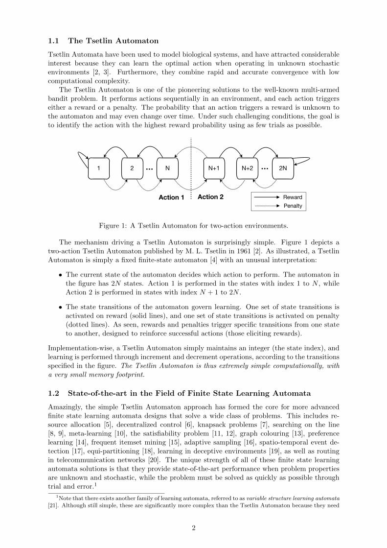
Figure 1: A Tsetlin Automaton for two-action environments.

The mechanism driving a Tsetlin Automaton is surprisingly simple. Figure 1 depicts atwo-action Tsetlin Automaton published by M. L. Tsetlin in 1961 [2]. As illustrated, a TsetlinAutomaton is simply a fixed finite-state automaton [4] with an unusual interpretation:

• The current state of the automaton decides which action to perform. The automaton inthe figure has 2N states. Action 1 is performed in the states with index 1 to N , whileAction 2 is performed in states with index N + 1 to 2N .

• The state transitions of the automaton govern learning. One set of state transitions isactivated on reward (solid lines), and one set of state transitions is activated on penalty(dotted lines). As seen, rewards and penalties trigger specific transitions from one stateto another, designed to reinforce successful actions (those eliciting rewards).

Implementation-wise, a Tsetlin Automaton simply maintains an integer (the state index), andlearning is performed through increment and decrement operations, according to the transitionsspecified in the figure. The Tsetlin Automaton is thus extremely simple computationally, witha very small memory footprint.

1.2 State-of-the-art in the Field of Finite State Learning Automata

Amazingly, the simple Tsetlin Automaton approach has formed the core for more advancedfinite state learning automata designs that solve a wide class of problems. This includes re-source allocation [5], decentralized control [6], knapsack problems [7], searching on the line[8, 9], meta-learning [10], the satisfiability problem [11, 12], graph colouring [13], preferencelearning [14], frequent itemset mining [15], adaptive sampling [16], spatio-temporal event de-tection [17], equi-partitioning [18], learning in deceptive environments [19], as well as routingin telecommunication networks [20]. The unique strength of all of these finite state learningautomata solutions is that they provide state-of-the-art performance when problem propertiesare unknown and stochastic, while the problem must be solved as quickly as possible throughtrial and error.1

1Note that there exists another family of learning automata, referred to as variable structure learning automata[21]. Although still simple, these are significantly more complex than the Tsetlin Automaton because they need

2

The ability to handle stochastic and unknown environments for a surprisingly wide range ofproblems, combined with its computational simplicity and small memory footprint, make theTsetlin Automaton an attractive building block for complex machine learning tasks. However,the success of the Tsetlin Automaton has been hindered by a particularly adverse challenge,explored by Kleinrock and Tung in 1996 [6]. Complex problem solving requires teams ofinteracting Tsetlin Automata, and unfortunately, each team member introduces noise. This isdue to the inherently decentralized and stochastic nature of Tsetlin Automata based decision-making. The automata independently decide upon their actions, directly based on the feedbackfrom the environment. This is on one hand a strength because it allows problems to be solvedin a decentralized manner. On the other hand, as the number of Tsetlin Automata grows, thelevel of noise increases. We refer to this effect as the vanishing signal-to-noise ratio problem.This vanishing signal-to-noise-ratio demands in the end an infinite number of states per TsetlinAutomaton, which in turn, leads to impractically slow convergence [3, 6].

0 0 * 1 * 0 0 0* 0 * 1 * 0 0 00 * * 1 * * * 00 * * * * 0 0 *0 0 0 * * 0 0 00 * 0 * * * 0 00 0 * 1 * * * 00 0 0 * 1 * * *

Table 1: A bit pattern produced by the Tsetlin Machine for handwritten digits ’1’. The ’*’symbol can either take the value ’0’ or ’1’. The remaining bit values require strict matching.The pattern is relatively easy to interpret for humans compared to, e.g., a neural network. It isalso efficient to evaluate for computers. Despite this simplicity, the Tsetlin Machine producesbit patterns that deliver state-of-the-art pattern recognition accuracy (see Section 5).

1.3 Paper Contributions

To attack the challenge of limited pattern expression capability and vanishing signal-to-noiseratio, in this paper we introduce the Tsetlin Machine. The contributions of the paper can besummarized as follows:

• The Tsetlin Machine solves complex pattern recognition problems with propositionalformulas, composed by a collective of Tsetlin Automata.

• We eliminate the longstanding vanishing signal-to-noise ratio problem with a uniquedecentralized learning scheme based on game theory. The game we have designed allowsthousands of Tsetlin Automata to successfully cooperate.

• Our theoretical analysis establishes that the Nash equilibria of the game are alignedwith the propositional formulas that provide optimal pattern recognition accuracy. Thistranslates to learning without local optima, only global ones.

• We further argue formally that the Tsetlin Machine finds the propositional formula thatprovides optimal pattern recognition accuracy, with probability arbitrarily close to unity.

• The game orchestrated by the Tsetlin Machine is based on resource allocation principles[7]. By allocating sparse pattern representation resources, the Tsetlin Machine is able

to maintain an action probability vector for sampling actions. Although promising, their success in patternrecognition has been limited to small scale problems, being restricted by constrained pattern representationcapability (linearly separable classes and simple decision trees) [21, 22, 3] and the problem of vanishing signal-to-noise-ratio [6], solved in the present paper.

3

to capture intricate unlabelled sub-patterns, for instance addressing the renowned NoisyXOR-problem.

• The propositional formulas are represented as bit patterns. These bit patterns are rel-atively easy to interpret, compared to e.g. a neural network (see Table 1 for a simpleexample bit pattern). This facilitates human quality assurance and scrutiny, which forinstance can be important in safety-critical domains such as medicine.

• The Tsetlin Machine is particularly suited for digital computers, being merely based onbit manipulation with AND-, OR-, and NOT operators. Both input, hidden patterns,and output are represented as bit patterns.

• In thorough empirical evaluations on four diverse datasets, the Tsetlin Machine outper-forms both single layer neural networks, Support Vector Machines, Random Forests, theNaive Bayes Classifier, and Logistic Regression.

• It further turns out that the Tsetlin Machine requires significantly less data than neuralnetworks, outperforming even the Naive Bayes Classifier in data sparse environments.

• We demonstrate how the Tsetlin Machine can be used as a building block to create moreadvanced architectures, including the Multi-Class Tsetlin Machine, the Fully ConnectedDeep Tsetlin Machine, the Convolutional Tsetlin Machine, and the Recurrent TsetlinMachine.

The combination of accuracy, interpretability, and computational simplicity makes the TsetlinMachine a promising tool for a wide range of domains, including safety-critical medicine. Beingthe first of its kind, we believe the Tsetlin Machine will kick-start completely new paths ofresearch, with a potentially significant impact on the field of AI and the applications of AI.

1.4 Paper Organization

The paper is organized as follows. In Section 2 we define the exact nature of the patternrecognition problem we are going to solve, also introducing the crucial concept of sub-patterns.

Then, in Section 3, we cover the Tsetlin Machine in detail. We first present the propositionallogic based pattern representation framework, before we introduce the Tsetlin Automata teamsthat write conjunctive clauses in propositional logic. These Tsetlin Automata teams are thenorganized to recognize complex patterns. We conclude the section by presenting the TsetlinMachine game that we use to coordinate thousands of Tsetlin Automata, eliminating thevanishing signal-to-noise ratio problem.

In Section 4 we analyse pertintent properties of the Tsetlin Machine formally, and establishthat the Nash equilibria of the game are aligned with the propositional formulas that solve thepattern recognition problem at hand. This allows the Tsetlin Machine as a whole to robustlyand accurately uncover complex patterns with propositional logic.

In our empirical evaluation in Section 5, we evaluate the performance of the Tsetlin Machineon four diverse data sets: Flower categorization, digit recognition, board game planning, andthe Noisy XOR Problem with Non-informative Features.

The Tsetlin Machine has been designed to act as a building block in more advanced ar-chitectures, and in Section 6 we demonstrate how four distinct architectures can be built byinterconnecting multiple Tsetlin Machines.

As the first step in a new research direction, the Tsetlin Machine also opens up a range ofnew research questions. In Section 7 we summarize our main findings and provide pointers tosome of the open research problems ahead.

2 The Pattern Recognition Problem

We here define the pattern recognition problem to be solved by the Tsetlin Machine, startingwith the input to the system. The input to the Tsetlin Machine is an observation vector

4

of o propositional variables, X = [x1, x2, . . . , xo] with xk ∈ {0,1}, 1 ≤ k ≤ o. From thisinput vector, the Tsetlin Machine is to produce an output vector Y = [y1, y2, . . . , yn] of npropositional variables, yi ∈ {0,1}, 1 ≤ i ≤ n.2

We assume that for each output, yi, 1 ≤ i ≤ n, an independent underlying stochasticprocesses of arbitrary complexity randomly produces either yi = 0 or yi = 1, from the in-put X = [x1, x2, . . . , xo]. To deal with the stochastic nature of these processes, we employprobability theory for reasoning and modelling.

In all brevity, uncertainty is fully captured by the probability P (yi = 1|X), that is, theprobability that yi takes the value 1 given the input X. Being binary, the probability that yi

takes the value 0 then follows: P (yi = 0|X) = 1− P (yi = 1|X).Under these conditions, the optimal decision is to assign yi the value v ∈ {0,1} with the

largest posterior probability[23]: argmaxv∈{0,1}P (yi = v|X).

P(yi = 0 | X ) > P(yi = 1 | X )

Sub-pattern Xi

Sub-pattern Xi

Sub-pattern Xi

Sub-pattern Xi

P(yi = 0 | X ) <= P(yi = 1 | X )

1

2

1

2

Figure 2: A partitioning of the input space according to the posterior probability of the outputvariable yi, highlighting distinct sub-patterns in the input space, X ∈ X . Sub-patterns mostlikely belonging to output yi = 1 can be found on the right side, while sub-patterns most likelybelonging to yi = 0 on the left.

Now consider the complete set of possible inputs, X = {x1, . . . , xo ∈ [0,1]o}. Each input Xoccurs with probability P (X), and thus the joint input-output distribution becomes P (X, yi) =P (yi|X)P (X).

As illustrated in Figure 2, the input space X can be partitioned in two parts, X i =

{X|P (yi = 0|X) ≤ P (yi = 1|X)} and X i= {X|P (yi = 0|X) > P (yi = 1|X)}. For ob-

servations in X i it is optimal to assign yi the value 1, while for partition X iit is optimal to

assign yi the value 0.We now come to the crucial concept of unlabelled sub-patterns. As illustrated in the figure,

X i sub-divides further into s sub-parts, forming distinct sub-patterns, X ir , r = 1, . . . , s (the

same goes for X i). Together, these sub-patterns span the whole input space, apart from a

minimal level of ”outlier” patterns that occur with probability, α, close to zero. That is,

P (X i1 ∪ . . . ∪ X i

s ∪ Xi1 ∪ . . . ∪ X

is) = 1.0− α, for a minimal α (the ”outliers” remaining after a

sub-division of the input space into s parts).However, we only observe samples (X, yi) from the joint input-output distribution P (X, yi).

Which sub-pattern X is sampled from is unavailable to us. We only know that each sub-patternX ir occurs with probability P (Xi

r) >1s (by definition).

2Note that we have decided to use the binary representation 0/1 to refer to the truth values False/True.These can be used interchangeably throughout the paper.

5

The challenging task we are going to solve is to learn all the sub-patterns merely by observinga limited sample from the joint input-output probability distribution P (X, yi), and by doing so,provide optimal pattern recognition accuracy.

3 The Tsetlin Machine

We now present the core concepts of the Tsetlin Machine in detail. We first present thepropositional logic based pattern representation framework, before we introduce the TsetlinAutomata teams that write conjunctive clauses in propositional logic. These Tsetlin Automatateams are then organized to recognize complex sub-patterns. We conclude the section bypresenting the Tsetlin Machine game that we use to coordinate thousands of Tsetlin Automata.

3.1 Expressing Patterns with Propositional Formulas

The accuracy of a machine learning technique is bounded by its pattern representation capa-bility. The Naive Bayes Classifier, for instance, assumes that input variables are independentgiven the output category [24]. When critical patterns cannot be fully represented by themachine learning technique, accuracy suffers. Unfortunately, compared to the representationcapability of the underlying language of digital computers, namely, Boolean algebra3, mostmachine learning techniques appear rather limited, with neural networks being one of the ex-ceptions. Indeed, with o input variables, X = [x1, x2, . . . , xo], there are no less than 22o uniquepropositional formulas, f(X). Perhaps only a single one of them will provide optimal patternrecognition accuracy for the task at hand.

We equip the Tsetlin Machine with the full expression power of propositional logic. Therepresentation power of propositional logic is perhaps best seen in light of the Satisfiabiliy(SAT) problem, which can be solved using a team of Tsetlin Automata [12]. The SAT problemis known to be NP-complete [25] and plays a central role in a number of applications in thefields of VLSI Computer-Aided design, Computing Theory, Theorem Proving, and ArtificialIntelligence. Generally, a SAT problem is defined in so-called conjunctive normal form. Tofacilitate Tsetlin Automata based learning, we will instead represent patterns using disjunctivenormal form.

Patterns in Disjunctive Normal Form. Briefly stated, we represent the relation be-tween an input, X = [x1, x2, . . . , xo], and the output, yi, using a propositional formula Φi indisjunctive normal form:

Φi =

m∨j=1

Cij . (1)

The formula consists of a disjunction of m conjunctive clauses, Cij . Each conjunctive clause in

turn, represents a specific sub-pattern governing the output yi.Sub-Patterns and Conjunctive Clauses. Each clause Ci

j in the propositional formula

Φi for yi has the form

Cij =

∧k∈Iij

xk

∧ ∧

k∈Iij

¬xk

. (2)

That is, the clause is a conjunction of literals, where a literal is a propositional variable, xk,without modification, or its negation ¬xk. Here, Iij and Iij are non-overlapping subsets of the

input variable indexes, Iij , Iij ⊆ {1, .....o}, Iij ∩ Iij = ∅. The subsets decide which of the input

variables take part in the clause, and whether they are negated or not. The input variablesfrom Iij are included as is, while the input variables from Iij are negated.

For example, the propositional formula (P ∧ ¬Q) ∨ (¬P ∧ Q) consists of two conjunctiveclauses, and four literals, P , Q, ¬P , and ¬Q. The formula evaluates to 1 if

3We found the Tsetlin Machine on propositional logic, which can be mapped to Boolean algebra, and viceversa.

6

• P = 1 and Q = 0, or if

• P = 0 and Q = 1.

All other truth value assignments evaluate to 0, and thus the formula captures the renownedXOR-relation.

Definition 1 (The Problem of Pattern Learning with Propositional Logic). A set S of inde-pendent samples, (X, yi), from the joint input-output probability distribution P (X, yi) is pro-vided. In the Problem of Pattern Learning with Propositional Logic, one must determine thepropositional formula Φi(X) that evaluates to 0 iff P (yi = 0|X) > P (yi = 1|X) and to 1 iffP (yi = 0|X) ≤ P (yi = 1|X), merely based on the samples in S.

The above problem decomposes into identifying the conjunctive clauses Cij whose disjunc-

tion evaluates to 1 iff X ∈ X i (see Section 2 for the definition of X i).

3.2 The Tsetlin Automata Team for Composing Clauses

At the core of the Tsetlin Machine we find the conjunctive clauses, Cij , j = 1, . . . ,m, from Eqn.

2. For each clause Cij , we form a team of 2o Tsetlin Automata, two Tsetlin Automata per

input variable xk. Figure 3 captures the role of each of these Tsetlin Automata, and how theyinteract to form the clause Ci

j .

TA1Exclude x1 Include x1

TA2Exclude ¬x1 Include ¬x1

TA2o-1Exclude xo Include xo

TA2oExclude ¬xo Include ¬xo

…

⌵ ⌵xu1 ¬ xu2 xuz

⌵ … ⌵

0 1 0 … 1 0 1Input

0/1Output

Figure 3: The Tsetlin Automata team for composing a clause.

As seen, o input variables, X = [x1, . . . , xo], are fed to the clause. The critical task of theTsetlin Automata team is to decide which input variables to include in Iij and which input

variables to include in Iij . If a literal is excluded by its associated Tsetlin Automaton, it doesnot take part in the conjunction. As illustrated in the figure, Tsetlin Automaton TA2k−1 isresponsible for deciding whether to ”Include” or ”Exclude” input variable xk, while anotherTsetlin Automaton, TA2k, decides whether to ”Include” or ”Exclude” ¬xk. That is, xk cantake part in the clause as is, take part in negated form, ¬xk, or not take part at all.

As illustrated to the right in the figure, the clause is formed after each Tsetlin Automatonhas made its decision, to include or exclude its associated literal. The current input X canthen be transformed to an output, using the clause, Ci

j(X) = xu1 ∧ ¬xu2 ∧ . . . ∧ xuz , that hasbeen formed by the automata team.

3.3 The Basic Tsetlin Machine Architecture

We are now ready to build the complete Tsetlin Machine. We do this by assigning m clauses,Cij , j = 1, 2, . . . ,m, to each output yi, i = 1, 2, . . . , n. The number of clauses m per output yi

is a meta-parameter that is decided by the number of sub-patterns associated with each yi. If

7

0/1

…

0/1

…

…⌵0/10/1

⌵

⌵ ⌵ ⌵ ⌵

0/1

0/1

1 0 0 … 1 0 1

Conjunctive Clauses

Disjunctions of Clauses

Input

Output

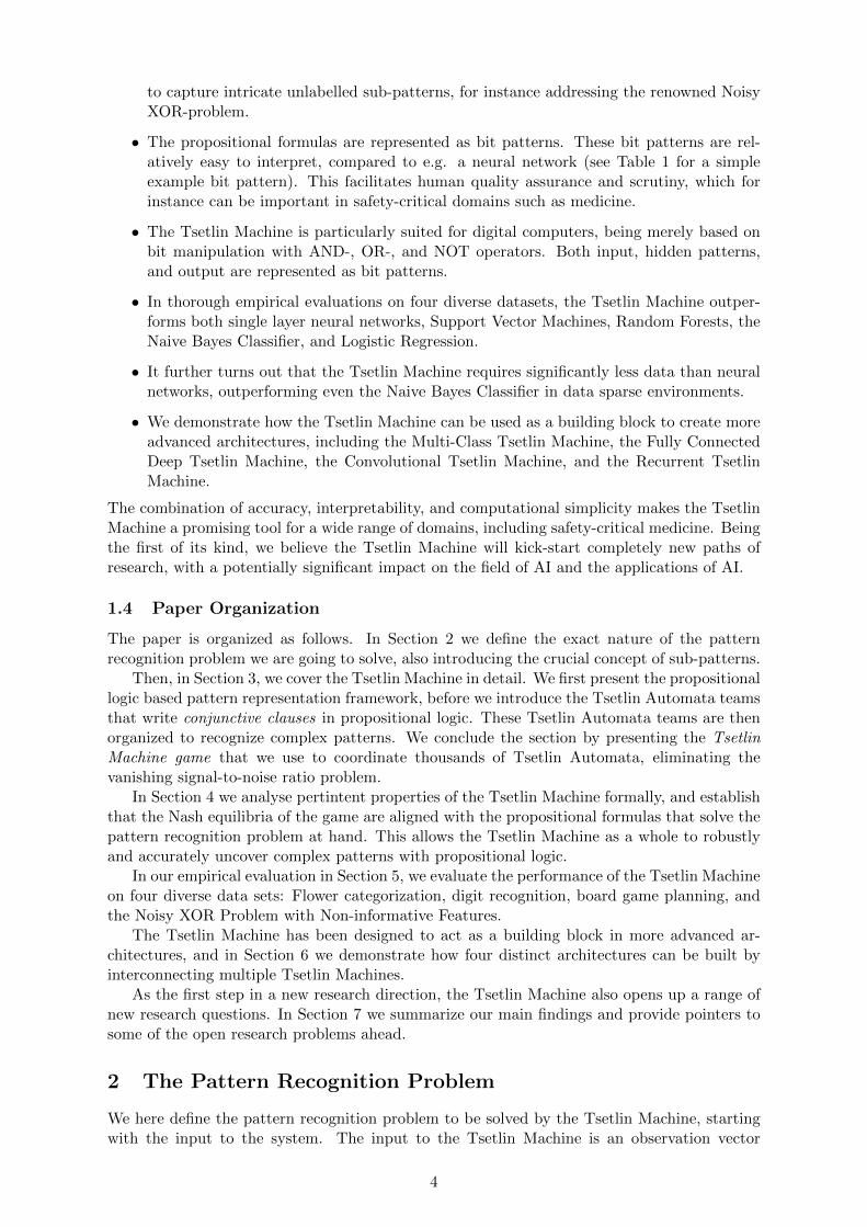
Figure 4: The basic Tsetlin Machine architecture.

0/1

… …

…

+ - + -

∑

⌵ ⌵ ⌵ ⌵

0 1 0 … 1 0 1

0/1

∑

0/1

0/1

0/10/1

Output

Input

Threshold Function

Summation

ConjunctiveClauses

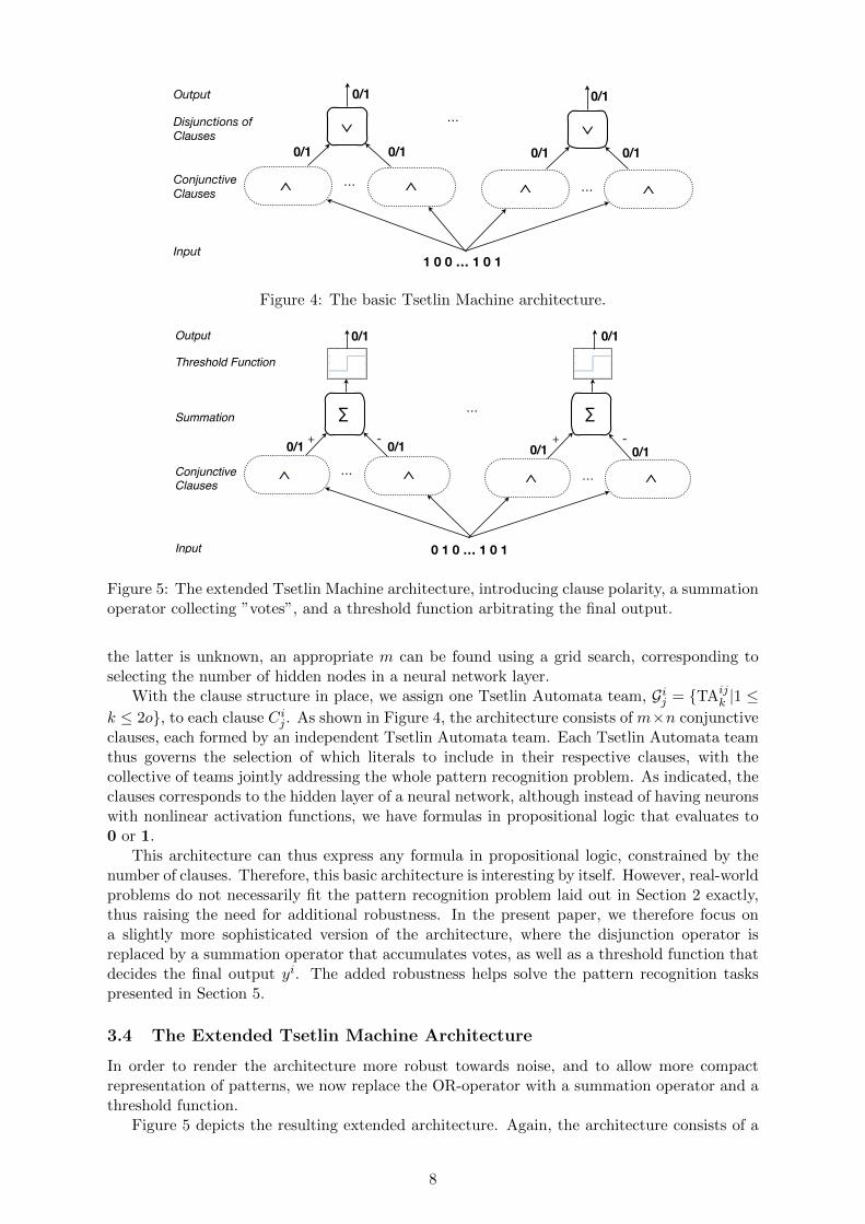
Figure 5: The extended Tsetlin Machine architecture, introducing clause polarity, a summationoperator collecting ”votes”, and a threshold function arbitrating the final output.

the latter is unknown, an appropriate m can be found using a grid search, corresponding toselecting the number of hidden nodes in a neural network layer.

With the clause structure in place, we assign one Tsetlin Automata team, Gij = {TAijk |1 ≤

k ≤ 2o}, to each clause Cij . As shown in Figure 4, the architecture consists of m×n conjunctive

clauses, each formed by an independent Tsetlin Automata team. Each Tsetlin Automata teamthus governs the selection of which literals to include in their respective clauses, with thecollective of teams jointly addressing the whole pattern recognition problem. As indicated, theclauses corresponds to the hidden layer of a neural network, although instead of having neuronswith nonlinear activation functions, we have formulas in propositional logic that evaluates to0 or 1.

This architecture can thus express any formula in propositional logic, constrained by thenumber of clauses. Therefore, this basic architecture is interesting by itself. However, real-worldproblems do not necessarily fit the pattern recognition problem laid out in Section 2 exactly,thus raising the need for additional robustness. In the present paper, we therefore focus ona slightly more sophisticated version of the architecture, where the disjunction operator isreplaced by a summation operator that accumulates votes, as well as a threshold function thatdecides the final output yi. The added robustness helps solve the pattern recognition taskspresented in Section 5.

3.4 The Extended Tsetlin Machine Architecture

In order to render the architecture more robust towards noise, and to allow more compactrepresentation of patterns, we now replace the OR-operator with a summation operator and athreshold function.

Figure 5 depicts the resulting extended architecture. Again, the architecture consists of a

8

number of conjunctive clauses, each associated with a dedicated Tsetlin Automata team thatdecides which literals to include in each clause. However, instead of simply taking part in anOR relation, each clause, Ci

j ∈ Ci = {Cij |j = 1, . . . ,m}, i ∈ {1, . . . , n}, is now given a fixed

polarity. For simplicity, we assign positive polarity to clauses with an odd index j, while clauseswith an even index are assigned negative polarity. In the figure, polarity is indicated with a’+’ or ’-’ sign, attached to the output of each clause.

Clauses, Cij , with positive polarity contribute to a final output of yi = 1, while clauses with

a negative polarity contribute towards a final output of yi = 0. The contributions can be seenas votes, with each clause either casting a vote, Ci

j(X) = 1, or declining to vote, Cij(X) = 0.

A positive vote means that the corresponding clause has recognized a sub-pattern associatedwith output yi = 1, while a negative vote means that the corresponding clause has recognizeda sub-pattern associated with the opposite output, yi = 0.

After the clauses has produced their output, a summation operator,∑

, associated with theoutput yi, sums the votes it receives from the clauses, Ci

j , j = 1, . . . ,m. Clauses with positivepolarity contribute positively while those with negative polarity contribute negatively. Overall,the purpose is to reach a balanced output decision, weighting positive evidence against negativeevidence (assuming m is even):

f∑(Ci(X)) =

∑j∈{1,3,...,m−1}

Cij(X)

− ∑

j∈{2,4,...,m}

Cij(X)

(3)

The final output, yi, is decided by a threshold function

ft(x) =

{0 for x < 0

1 for x ≥ 0.

that outputs 1 if the outcome of the summation is larger than or equal to zero. Otherwise,it outputs 0. The final output yj can thus be calculated directly from an input X simply bysumming the signed output of the m conjunctive clauses, followed by activating the thresholdfunction:

yi = ft(f∑(Ci(X))). (4)

As a result of the expression power of propositional logic, highly complex patterns can becaptured by the Tsetlin Machine. Furthermore, it is arguably easier for humans to interpretpropositional formula compared to a neural network. Finally, notice how all of the operatorsare highly suited for the digital circuits of modern computers.

The crucial remaining issue, then, is how to learn the conjunctive clauses from data, toobtain optimal pattern recognition accuracy. We attack this problem next.

3.5 The Tsetlin Machine Game for Learning Conjunctive Clauses

We here introduce a novel game theoretic learning mechanism that guides the Tsetlin Automatastochastically towards solving the pattern recognition problem from Definition 1. The game isdesigned to deal with the problem of vanishing signal-to-noise ratio for large Tsetlin Automatateams that contain thousands of Tsetlin Automata.

The complexity of the Tsetlin Machine game is immense, because the decisions of everysingle Tsetlin Automaton jointly decide the behaviour of the Tsetlin Machine as a whole. In-deed, a single Tsetlin Automaton has the power to completely disrupt a clause by introducing acontradiction. The payoffs of the game must therefore be designed carefully, so that the TsetlinAutomata are guided in the correct direction. To complicate further, an explicit enumerationof the payoffs is impractical due to the potentially tremendous size of the game matrix. Instead,the payoffs associated with each cell must be calculated on demand.

9

3.5.1 Design of the Payoff Matrix

We design the payoff matrix for the game based on the notion of:

• True positive output. We define true positive output as correctly providing outputyi = 1.

• False negative output. We define false negative output as incorrectly providing theoutput yi = 0 when the output should have been yi = 1.

• False positive output. We define false positive output as incorrectly providing theoutput yi = 1 when the output should have been yi = 0.

By progressively reducing false negative and false positive output, and reinforcing true positiveoutput, we intend to guide the Tsetlin Automata towards optimal pattern recognition accuracy.This guiding is based on what we will refer to as Type I and Type II Feedback.

3.5.2 Type I Feedback – Combating False Negative Output

Type I Feedback is decided by two factors, connecting the players of the game together:

• The choices of the Tsetlin Automata team Gij as a whole, summarized by the output of

the clause Cij(X) (the truth value of the clause).

• The truth value of the literal xk/¬xk assigned to the Tsetlin Automaton TAij2k−1/TAij

2k.

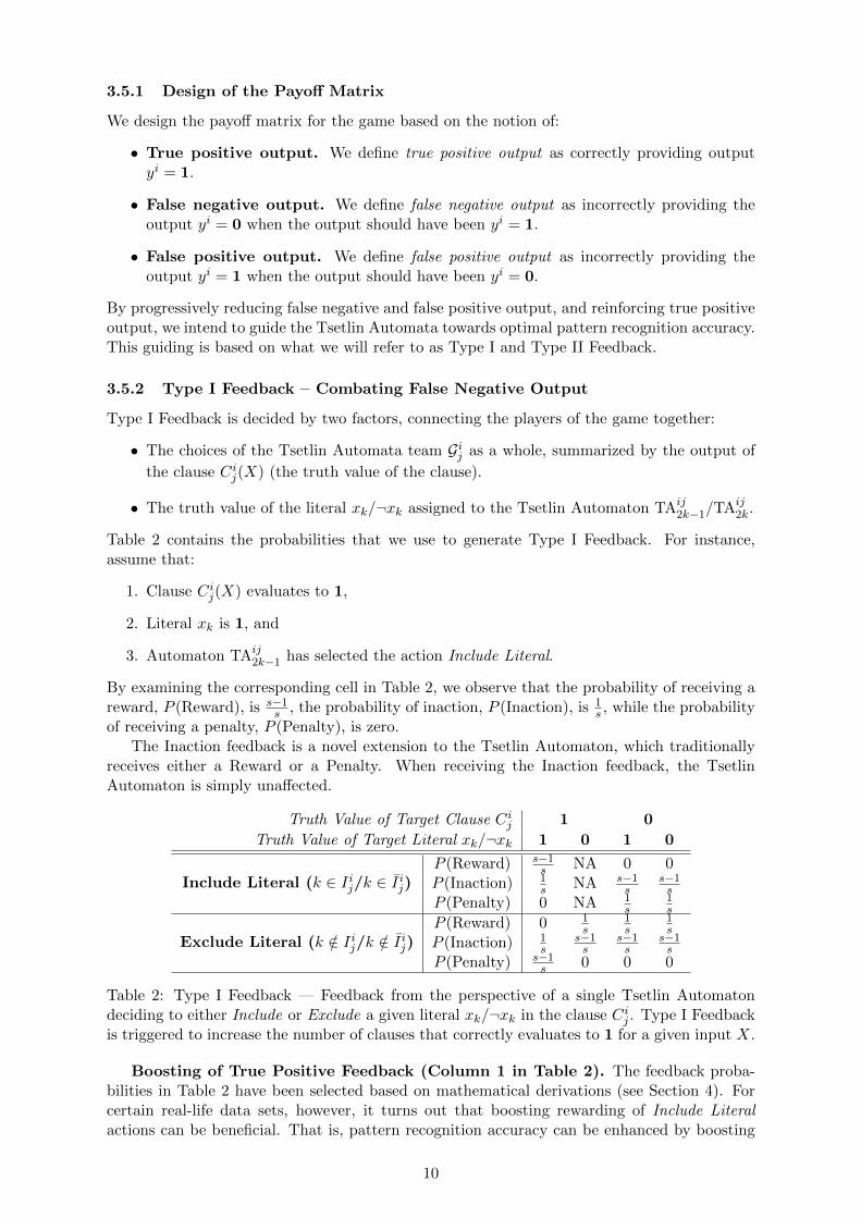
Table 2 contains the probabilities that we use to generate Type I Feedback. For instance,assume that:

1. Clause Cij(X) evaluates to 1,

2. Literal xk is 1, and

3. Automaton TAij2k−1 has selected the action Include Literal.

By examining the corresponding cell in Table 2, we observe that the probability of receiving areward, P (Reward), is s−1

s , the probability of inaction, P (Inaction), is 1s , while the probability

of receiving a penalty, P (Penalty), is zero.The Inaction feedback is a novel extension to the Tsetlin Automaton, which traditionally

receives either a Reward or a Penalty. When receiving the Inaction feedback, the TsetlinAutomaton is simply unaffected.

Truth Value of Target Clause Cij 1 0

Truth Value of Target Literal xk/¬xk 1 0 1 0

Include Literal (k ∈ Iij/k ∈ Iij)P (Reward) s−1

s NA 0 0P (Inaction) 1

s NA s−1s

s−1s

P (Penalty) 0 NA 1s

1s

Exclude Literal (k /∈ Iij/k /∈ Iij)P (Reward) 0 1

s1s

1s

P (Inaction) 1s

s−1s

s−1s

s−1s

P (Penalty) s−1s 0 0 0

Table 2: Type I Feedback — Feedback from the perspective of a single Tsetlin Automatondeciding to either Include or Exclude a given literal xk/¬xk in the clause Ci

j . Type I Feedbackis triggered to increase the number of clauses that correctly evaluates to 1 for a given input X.

Boosting of True Positive Feedback (Column 1 in Table 2). The feedback proba-bilities in Table 2 have been selected based on mathematical derivations (see Section 4). Forcertain real-life data sets, however, it turns out that boosting rewarding of Include Literalactions can be beneficial. That is, pattern recognition accuracy can be enhanced by boosting

10

rewarding of these actions when they produce true positive outcomes. Penalizing of ExcludeLiteral actions is then adjusted accordingly. In all brevity, we boost rewarding in this mannerby replacing s−1

s with 1.0 and 1s with 0.0 in Column 1 of Table 2.

Brief analysis of the Type I Feedback. Notice how the reward probabilities are de-signed to ”tighten” clauses up to a certain point. That is, the probability of receiving rewardswhen selecting Include Literal is larger than when selecting Exclude Literal. The ratio is con-trolled by the parameter s. In this manner, s effectively decides how ”fine grained” patterns theclauses are going to capture. The larger the value of s, the more the Tsetlin Automata teamis stimulated to include literals in the clause. The only countering force is the inputs, X, thatdo not match the clause, which obviously grows as s is increased (the clause is ”tightened”).When these forces are in balance, we have a Nash equilibrium as discussed further in the nextsection.

The above mechanism is a critical part of the Tsetlin Machine, allowing learning of anysub-pattern Xi

j , no matter how infrequent, as long as P (Xij) is larger than 1

s . This novelmechanism is studied both theoretically and empirically in the two following sections. As arule of thumb, a large s leads to more ”fine grained” clauses, that is, clauses with more literals,while a small s produces ”coarser” clauses, with less literals included.

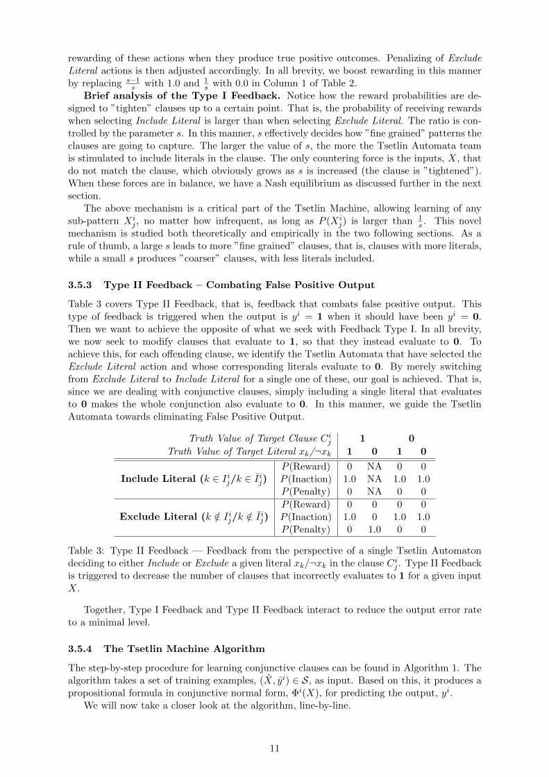
3.5.3 Type II Feedback – Combating False Positive Output

Table 3 covers Type II Feedback, that is, feedback that combats false positive output. Thistype of feedback is triggered when the output is yi = 1 when it should have been yi = 0.Then we want to achieve the opposite of what we seek with Feedback Type I. In all brevity,we now seek to modify clauses that evaluate to 1, so that they instead evaluate to 0. Toachieve this, for each offending clause, we identify the Tsetlin Automata that have selected theExclude Literal action and whose corresponding literals evaluate to 0. By merely switchingfrom Exclude Literal to Include Literal for a single one of these, our goal is achieved. That is,since we are dealing with conjunctive clauses, simply including a single literal that evaluatesto 0 makes the whole conjunction also evaluate to 0. In this manner, we guide the TsetlinAutomata towards eliminating False Positive Output.

Truth Value of Target Clause Cij 1 0

Truth Value of Target Literal xk/¬xk 1 0 1 0

Include Literal (k ∈ Iij/k ∈ Iij)P (Reward) 0 NA 0 0P (Inaction) 1.0 NA 1.0 1.0P (Penalty) 0 NA 0 0

Exclude Literal (k /∈ Iij/k /∈ Iij)P (Reward) 0 0 0 0P (Inaction) 1.0 0 1.0 1.0P (Penalty) 0 1.0 0 0

Table 3: Type II Feedback — Feedback from the perspective of a single Tsetlin Automatondeciding to either Include or Exclude a given literal xk/¬xk in the clause Ci

j . Type II Feedbackis triggered to decrease the number of clauses that incorrectly evaluates to 1 for a given inputX.

Together, Type I Feedback and Type II Feedback interact to reduce the output error rateto a minimal level.

3.5.4 The Tsetlin Machine Algorithm

The step-by-step procedure for learning conjunctive clauses can be found in Algorithm 1. Thealgorithm takes a set of training examples, (X, yi) ∈ S, as input. Based on this, it produces apropositional formula in conjunctive normal form, Φi(X), for predicting the output, yi.

We will now take a closer look at the algorithm, line-by-line.

11

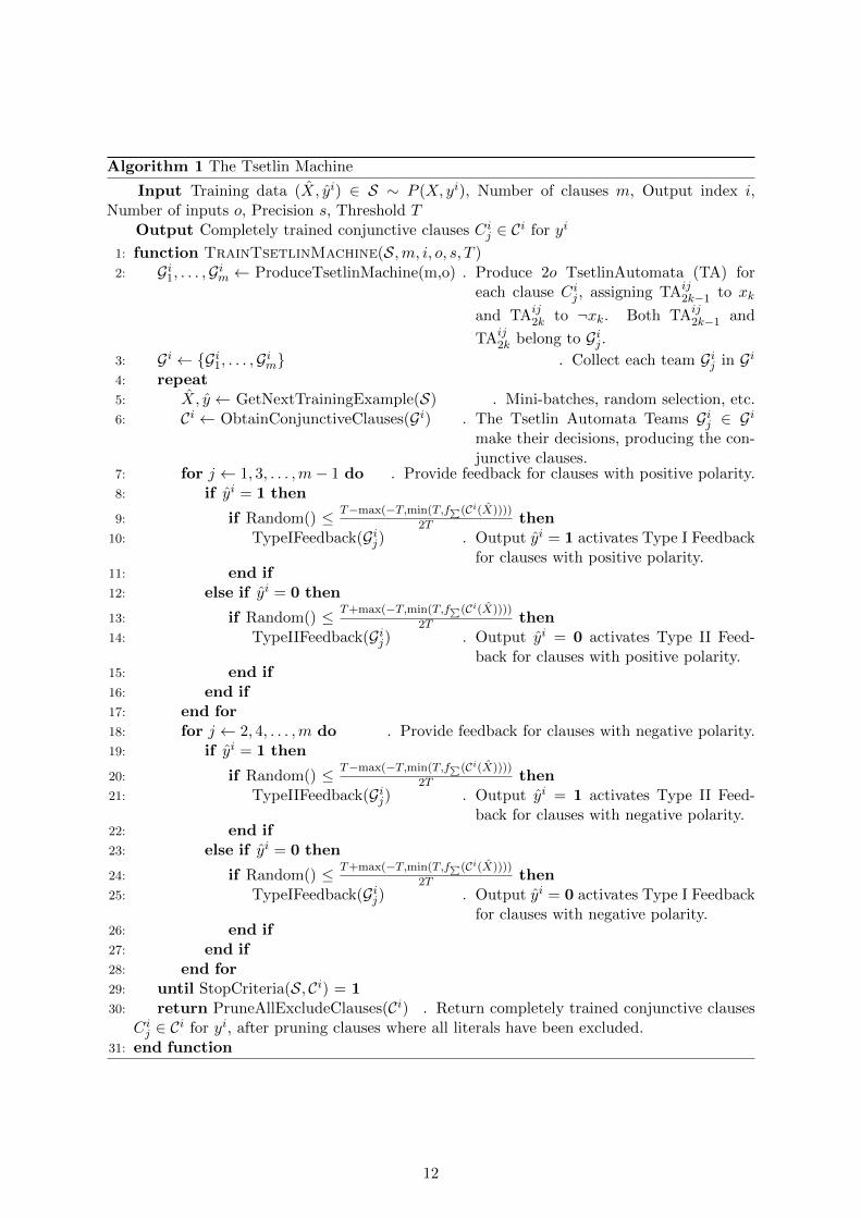
Algorithm 1 The Tsetlin Machine

Input Training data (X, yi) ∈ S ∼ P (X, yi), Number of clauses m, Output index i,Number of inputs o, Precision s, Threshold T

Output Completely trained conjunctive clauses Cij ∈ Ci for yi

1: function TrainTsetlinMachine(S,m, i, o, s, T )2: Gi1, . . . ,Gim ← ProduceTsetlinMachine(m,o) . Produce 2o TsetlinAutomata (TA) for

each clause Cij , assigning TAij

2k−1 to xk

and TAij2k to ¬xk. Both TAij

2k−1 and

TAij2k belong to Gij .

3: Gi ← {Gi1, . . . ,Gim} . Collect each team Gij in Gi4: repeat5: X, y ← GetNextTrainingExample(S) . Mini-batches, random selection, etc.6: Ci ← ObtainConjunctiveClauses(Gi) . The Tsetlin Automata Teams Gij ∈ Gi

make their decisions, producing the con-junctive clauses.

7: for j ← 1, 3, . . . ,m− 1 do . Provide feedback for clauses with positive polarity.8: if yi = 1 then

9: if Random() ≤ T−max(−T,min(T,f∑(Ci(X))))

2T then10: TypeIFeedback(Gij) . Output yi = 1 activates Type I Feedback

for clauses with positive polarity.11: end if12: else if yi = 0 then

13: if Random() ≤ T+max(−T,min(T,f∑(Ci(X))))

2T then14: TypeIIFeedback(Gij) . Output yi = 0 activates Type II Feed-

back for clauses with positive polarity.15: end if16: end if17: end for18: for j ← 2, 4, . . . ,m do . Provide feedback for clauses with negative polarity.19: if yi = 1 then

20: if Random() ≤ T−max(−T,min(T,f∑(Ci(X))))

2T then21: TypeIIFeedback(Gij) . Output yi = 1 activates Type II Feed-

back for clauses with negative polarity.22: end if23: else if yi = 0 then

24: if Random() ≤ T+max(−T,min(T,f∑(Ci(X))))

2T then25: TypeIFeedback(Gij) . Output yi = 0 activates Type I Feedback

for clauses with negative polarity.26: end if27: end if28: end for29: until StopCriteria(S, Ci) = 130: return PruneAllExcludeClauses(Ci) . Return completely trained conjunctive clauses

Cij ∈ Ci for yi, after pruning clauses where all literals have been excluded.

31: end function

12

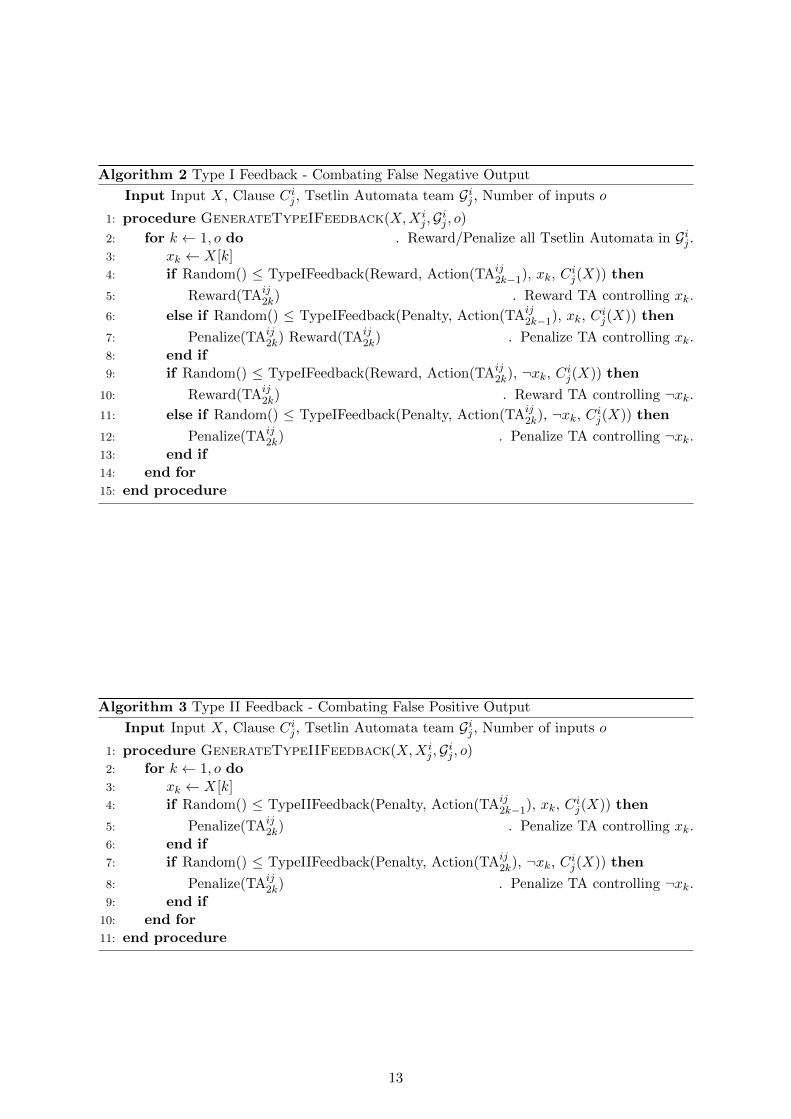
Algorithm 2 Type I Feedback - Combating False Negative Output

Input Input X, Clause Cij , Tsetlin Automata team Gij , Number of inputs o

1: procedure GenerateTypeIFeedback(X,Xij ,Gij , o)

2: for k ← 1, o do . Reward/Penalize all Tsetlin Automata in Gij .3: xk ← X[k]4: if Random() ≤ TypeIFeedback(Reward, Action(TAij

2k−1), xk, Cij(X)) then

5: Reward(TAij2k) . Reward TA controlling xk.

6: else if Random() ≤ TypeIFeedback(Penalty, Action(TAij2k−1), xk, Ci

j(X)) then

7: Penalize(TAij2k) Reward(TAij

2k) . Penalize TA controlling xk.8: end if9: if Random() ≤ TypeIFeedback(Reward, Action(TAij

2k), ¬xk, Cij(X)) then

10: Reward(TAij2k) . Reward TA controlling ¬xk.

11: else if Random() ≤ TypeIFeedback(Penalty, Action(TAij2k), ¬xk, Ci

j(X)) then

12: Penalize(TAij2k) . Penalize TA controlling ¬xk.

13: end if14: end for15: end procedure

Algorithm 3 Type II Feedback - Combating False Positive Output

Input Input X, Clause Cij , Tsetlin Automata team Gij , Number of inputs o

1: procedure GenerateTypeIIFeedback(X,Xij ,Gij , o)

2: for k ← 1, o do3: xk ← X[k]4: if Random() ≤ TypeIIFeedback(Penalty, Action(TAij

2k−1), xk, Cij(X)) then

5: Penalize(TAij2k) . Penalize TA controlling xk.

6: end if7: if Random() ≤ TypeIIFeedback(Penalty, Action(TAij

2k), ¬xk, Cij(X)) then

8: Penalize(TAij2k) . Penalize TA controlling ¬xk.

9: end if10: end for11: end procedure

13

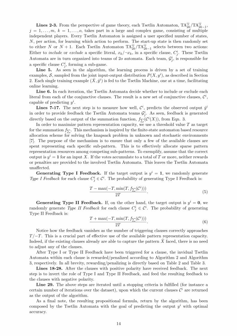
Lines 2-3. From the perspective of game theory, each Tsetlin Automaton, TAij2k/TAij

2k−1,j = 1, . . . ,m, k = 1, . . . , o, takes part in a large and complex game, consisting of multipleindependent players. Every Tsetlin Automaton is assigned a user specified number of states,N , per action, for learning which action to perform. The start-up state is then randomly setto either N or N + 1. Each Tsetlin Automaton TAij

2k/TAij2k−1 selects between two actions:

Either to include or exclude a specific literal, xk/¬xk, in a specific clause, Cij . These Tsetlin

Automata are in turn organized into teams of 2o automata. Each team, Gij , is responsible for

a specific clause Cij , forming a sub-game.

Line 5. As seen in the algorithm, the learning process is driven by a set of trainingexamples, S, sampled from the joint input-output distribution P (X, yi), as described in Section2. Each single training example (X, yi) is fed to the Tsetlin Machine, one at a time, facilitatingonline learning.

Line 6. In each iteration, the Tsetlin Automata decide whether to include or exclude eachliteral from each of the conjunctive clauses. The result is a new set of conjunctive clauses, Ci,capable of predicting yi.

Lines 7-17. The next step is to measure how well, Ci, predicts the observed output yi

in order to provide feedback the Tsetlin Automata teams Gij . As seen, feedback is generated

directly based on the output of the summation function, f∑(Ci(X)), from Eqn. 3.In order to maximize pattern representation capacity, we use a threshold value T as target

for the summation f∑. This mechanism is inspired by the finite-state automaton based resourceallocation scheme for solving the knapsack problem in unknown and stochastic environments[7]. The purpose of the mechanism is to ensure that only a few of the available clauses arespent representing each specific sub-pattern. This is to effectively allocate sparse patternrepresentation resources among competing sub-patterns. To exemplify, assume that the correctoutput is yi = 1 for an input X. If the votes accumulate to a total of T or more, neither rewardsor penalties are provided to the involved Tsetlin Automata. This leaves the Tsetlin Automataunaffected.

Generating Type I Feedback. If the target output is yi = 1, we randomly generateType I Feedback for each clause Ci

j ∈ Ci. The probability of generating Type I Feedback is:

T −max(−T,min(T, f∑(Ci)))2T

. (5)

Generating Type II Feedback. If, on the other hand, the target output is yi = 0, werandomly generate Type II Feedback for each clause Ci

j ∈ Ci. The probability of generatingType II Feedback is:

T + max(−T,min(T, f∑(Ci)))2T

. (6)

Notice how the feedback vanishes as the number of triggering clauses correctly approachesT/−T . This is a crucial part of effective use of the available pattern representation capacity.Indeed, if the existing clauses already are able to capture the pattern X faced, there is no needto adjust any of the clauses.

After Type I or Type II Feedback have been triggered for a clause, the invidual TsetlinAutomata within each clause is rewarded/penalized according to Algorithm 2 and Algorithm3, respectively. In all brevity, rewarding/penalizing is directly based on Table 2 and Table 3.

Lines 18-28. After the clauses with positive polarity have received feedback. The nextstep is to invert the role of Type I and Type II Feedback, and feed the resulting feedback tothe clauses with negative polarity.

Line 29. The above steps are iterated until a stopping criteria is fulfilled (for instance acertain number of iterations over the dataset), upon which the current clauses Ci are returnedas the output of the algorithm.

As a final note, the resulting propositional formula, return by the algorithm, has beencomposed by the Tsetlin Automata with the goal of predicting the output yi with optimalaccuracy.

14

4 Theoretical Analysis

The reader may now have recognized that we have designed the Tsetlin Machine with mathe-matical analysis in mind, in order to facilitate a deeper understanding of our learning scheme.In this section, we argue that the Tsetlin Machine converges towards solving the problem ofPattern Learning with Propositional Logic from Definition 1 with probability arbitrary closeto unity.

Assume that the propositional formula Φi for output yi solves a given pattern recognitionproblem, per Definition 1. Let X i = {X|Φi(X) = 1, X ∈ X} be the subset of input values

X that makes Φi evaluate to 1. Furthermore, let X i= {X|Φi(X) = 0, X ∈ X} be the

complement of X i. Let lk be a literal referring to either xk or ¬xk. Now consider one of theconjunctive clauses, Ci

j , that takes part in Φi. Let X ij = {X|Ci

j(X) = 1, X ∈ X i} and let

X i∗j = {X|Ci

j(X) = 1 ∧ lk = 1, X ∈ X i}.Further, let the subgame involving the Tsetlin Automata that form the clause Ci

j(X) be

denoted by Gij = {TAijk |1 ≤ k ≤ 2o}. Consider one of the Tsetlin Automata TAij

k ∈ Gij in the

subgame Gij . The payoffs it can receive are given in Table 2 and Table 3 for the whole range

of subgame Gij outcomes, from the perspective of TAijk . Finally, let (X, yi) be an input-output

pair sampled from P (X, yi).

Lemma 1. The expected payoff of the action Exclude Literal within the subgame Gij is:

P (X ∈ X i \ X i∗j |yi = 1)P (yi = 1) · 1

s+ P (X ∈ X i|yi = 1)P (yi = 1) · 1

s−

P (X ∈ X i∗j |yi = 1)P (yi = 1) · s− 1

s− P (X ∈ X i

j \ X i∗j |yi = 0)P (yi = 0) · 1.0 (7)

Proof. In brief, we receive an expected fractional reward 1s every time yi becomes 1, except

when both lk and Ci∗j (X) in Φi evaluates to 1. In that case, we instead receive an expected

fractional penalty of s−1s (see Table 2). Formally, we can reformulate this rewarding and

penalizing as follows:

P (yi = 1 ∧ ¬(Cij(X) = 1 ∧ lk = 1)) · 1

s− P (yi = 1 ∧ Ci

j(X) = 1 ∧ lk = 1) · s− 1

s= (8)

P (yi = 1 ∧ ¬(X ∈ X i∗j )) · 1

s− P (yi = 1 ∧X ∈ X i∗

j ) · s− 1

s= (9)

P (yi = 1 ∧X ∈ X i∗j ) · 1

s− P (yi = 1 ∧X ∈ X i∗

j ) · s− 1

s= (10)

P (yi = 1 ∧X ∈ X i \ X i∗j ) · 1

s+ P (yi = 1 ∧X ∈ X i

) · 1

s−

P (yi = 1 ∧X ∈ X i∗j ) · s− 1

s= (11)

P (X ∈ X i \ X i∗j |yi = 1)P (yi = 1) · 1

s+ P (X ∈ X i|yi = 1)P (yi = 1) · 1

s−

P (X ∈ X i∗j |yi = 1)P (yi = 1) · s− 1

s(12)

Furthermore, selecting the Exclude Literal when lk = 0 and yi = 0, while Cij(X) evaluates

to 1, provides a full penalty (see Table 3). As further seen in the table, false positive outputnever triggers penalties or rewards for the Include Literal action. All this is by design inorder to suppress the output 1 from Ci

j(X) in such cases. In other words, an even strongerNash equilibrium exists when switching from Include Literal to Exclude Literal increases theprobability of false positive output. This additional effect which enforces the Nash equilibriumcan be formalized as follows:

P (yi = 0 ∧ lk = 0 ∧ Cij(X) = 1) · 1.0 = (13)

P (X ∈ X ij \ X i∗

j |yi = 0)P (yi = 0) · 1.0 (14)

15

Lemma 2. The expected payoff of the action Include Literal within the subgame Gij is:

P (X ∈ X i∗j |yi = 1)P (yi = 1) · s− 1

s−

P (X ∈ X i \ X i∗j |yi = 1)P (yi = 1) · 1

s+ P (X ∈ X i|yi = 1)P (yi = 1) · 1

s(15)

Proof. We now simply establish that the expected feedback of action Include Literal is sym-metric to the expected feedback of action Exclude Literal, apart from not being affected byType II Feedback.

P (yi = 1 ∧ Cij(X) = 1) · s− 1

s− P (yi = 1 ∧ ¬Ci

j(X) = 1) · 1

s= (16)

P (yi = 1 ∧ Cij(X) = 1 ∧ lk = 1) · s− 1

s− P (yi = 1 ∧ ¬(Ci

j(X) = 1 ∧ lk = 1)) · 1

s= (17)

P (yi = 1 ∧X ∈ X i∗j ) · s− 1

s− P (yi = 1 ∧X ∈ X i∗

j ) · 1

s(18)

As seen above, we verify symmetry by observing that the action Include Literal with Cij(X) = 1

enforces lk = 1. This in turn allows us to replace Cij(X) = 1 with X ∈ X i

j . Together withthe obvious symmetry of Table 3, this makes the expected payoff symmetric to that of ExcludeLiteral (apart from the Type II Feedback) .

In other words, for the same reasons that Exclude Literal has a negative expected payoff,Include Literal has a positive one, and vice versa! This symmetry is by design to facilitaterobust and fast learning in the game.

Theorem 1. Let Φi be a solution to a pattern recognition problem per Definition 1. Thenevery clause Ci

j in Φi is a Nash equilibrium in the associated Tsetlin Machine subgame Gij.

Proof. We now have two scenarios. Either the literal lk is part of the clause Cij in the solution

Φi (the action selected by TAijk is Include Literal). Otherwise, the literal is not part of the

clause Cij in the solution Φi (the selected action is Exclude Literal). We will now consider each

of these scenarios for Φi, and verify that both scenarios qualify as Nash equilibria.Scenario 1: Literal included. A literal lk is included in a clause Ci

j for two reasons:

1. To provide a certain granularity 1s of Ci

j , i.e., to maintain P (Cij(X)) = 1

s + ε for as smallas possible ε > 0.

2. To combat false positive output Cij(X) = 1 when y = 0, by including literals lk that

makes Cij(X) evaluate to 0 whenever y = 0.

Consider the expected payoff of Exclude Literal :

P (X ∈ X i \ X i∗j |yi = 1)P (yi = 1) · 1

s+ P (X ∈ X i|yi = 1)P (yi = 1) · 1

s−

P (X ∈ X i∗j |yi = 1)P (yi = 1) · s− 1

s− P (X ∈ X i

j \ X i∗j |yi = 0)P (yi = 0) · 1.0 (19)

Let us first consider the situation where P (X ∈ X i|yi = 1)P (yi = 1) is zero. This means thatwe only obtain yi = 1 when the input belongs to X i. Then we only need to consider:

P (X ∈ X i \ X i∗j |yi = 1)P (yi = 1) · 1

s−

P (X ∈ X i∗j |yi = 1)P (yi = 1) · s− 1

s− P (X ∈ X i

j \ X i∗j |yi = 0)P (yi = 0) · 1.0 (20)

Since P (X ∈ X i∗j |yi = 1) > 1

s and P (X ∈ X i \ X i∗j |yi = 1) < s−1

s by definition, the expected

payoff for Exclude Literal is negative for this reason alone. Another important task of TAijk ∈ G

ij

16

is to combat false positive output, which happens when yi is 0 while Cij(X) evaluates to 1.

To achieve this, selecting the Exclude Literal when lk = 0 and yi = 0, while Ci∗j (X) evaluates

to 1, triggers a full penalty (see Table 3). In other words, the Nash equilibrium is further”strengthened” by potential false positive output.

Let us now return to the more general case of α = P (X ∈ X i|yi = 1) being greater thanor equal to zero. Then we have P (X ∈ X i∗

j |yi = 1) > (1 − α) · 1s and P (X ∈ X i \ X i∗

j |yi =

1) < (1− α) · s−1s by definition. Additionally, we now alse get the expected reward α · 1

s . Thelatter reward shifts the equilibrium towards Exclude Literal, which can be compensated forby artificially increasing s, to keep the expected payoff for Exclude Literal negative. In otherwords, by manipulating s we can achieve the intended Nash equilibrium, even with extremenoise.

Recall that the whole purpose of the above Nash equilibrium is to make sure that the pat-terns captured by the clause Ci

j is of an appropriate granularity, decided by s, finely balancingExclude Literal actions against Include Literal actions. This is combined with the combatingof false positive output through targeted selection of Include Literal actions.

To conclude, due to the established symmetry in payoff, switching from Include Literal toExclude Literal leads to a net loss in expected payoff, providing a Nash equilibrium for theaction Include Literal.

Scenario 2: Literal excluded. A literal lk is excluded from a clause Cij for one reason:

To maintain P (Cij(X)) = 1

s + ε for as small as possible ε > 0, i.e., to maintain a certain

granularity for the patterns matched by Cij . Again, consider the expected payoff of Exclude

Literal when P (X ∈ X i|yi = 1) is zero:

P (X ∈ X i \ X i∗j |yi = 1)P (yi = 1) · 1

s−

P (X ∈ X i∗j |yi = 1)P (yi = 1) · s− 1

s− P (X ∈ X i

j \ X i∗j |yi = 0)P (yi = 0) · 1.0 (21)

We know that P (X ∈ X ij \ X i∗

j |yi = 0)P (yi = 0) · 1.0 is minimal since Φi is a solution. For the

same reason, we know that P (X ∈ X i∗j |yi = 1) ≤ 1

s if P (X ∈ X ij |yi = 1) = 1

s + ε. This again,

implies that P (X ∈ X i \ X i∗j |yi = 1) > s−1

s . In other words, the expected payoff of ExcludeLiteral is positive, which due to the symmetry again means that Include Literal has a negative

expected payoff. For the case where P (X ∈ X i|yi = 1) is greater than zero, we can apply thesame reasoning as in Scenario 1. Hence, the Nash equilibrium!

Theorem 2 (A conjunctive Cij that is not part of the solution Φi is not a Nash equilibrium).

Proof. This theorem follows from the proof for Theorem 1. By invalidating any of the requiredconditions that made a clause Ci

j a Nash equilibrium, it can no longer be a Nash equilibrium.

Theorem 3. The Tsetlin Machine converges to a solution Φi with probability arbirtrarily closeto unity.

Proof. Here follows a sketch for a proof. Any solution scheme that is capable of finding asingle Nash equilibrium in a game will be able to solve each subgame Gij . Each subgame Gij isplayed independently of the other subgames, apart from the indirect interaction through thesummation function f∑. However, the feedback that connects the subgames only control howoften each game is activated. Indeed, a subgame is activated with probability

T −max(−T,min(T, f∑(Ci)))2T

(22)

for Type I Feedback, and with probability:

T + max(−T,min(T, f∑(Ci)))2T

(23)

17

for Type II Feedback. These together merely control the mixing factor of the two different typesof feedback, as well as the frequency with which the subgame is played. Type II Feedback isself-defeating, eliminating itself by nature to a minimum. As an equilibrium is found in eachsubgame, eventually, all subgames are stopped playing, i.e. f∑(Ci) always evaluates to eitherT or −T , and the Tsetlin Machine Game has been solved.

The Tsetlin Automaton is one particularly robust mechanism for solving games with com-mon payoff, converging to a Nash equilibrium with probability arbitrarily close to unity.

5 Empirical Results

In this section we evaluate the Tsetlin Machine empirically using four diverse datasets4:

• Binary Iris Dataset. This is the classical Iris Dataset, however, with features in binaryform.

• Binary Digits Dataset. This is the classical digits dataset, again with features inbinary form.

• Axis & Allies Board Game Dataset. This new dataset is designed to be a challengingmachine learning benchmark, involving optimal move prediction in a minimalistic, yetintricate, mini-game from the Axis & Allies board game.

• Noisy XOR Dataset with Non-informative Features. This artificial dataset isdesigned to reveal particular ”blind zones” of pattern recognition algorithms. The datasetcaptures the renowned XOR-relation. Furthermore, the dataset contains a large numberof random non-informative features to measure susceptibility towards the so-called Curseof Dimensionality [26]. To examine robustness towards noise we have further randomlyinverted 40% of the outputs.

For these datasets, we performed ensembles of 100 to 1000 independent replications withdifferent random number streams. We did this to minimize the variance of the reported results,to avoid being deceived by random variation, and to provide the foundation for a statisticalanalysis of the merits of the different schemes evaluated.

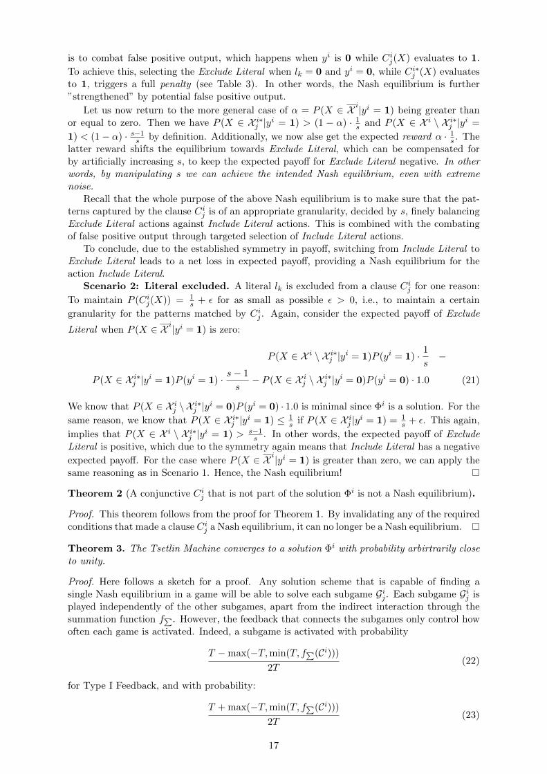
Together with the Tsetlin Machine, we have also evaluated several classical machine learningtechniques using the same random number streams. This includes Neural Networks, the NaiveBayes Classifier, Support Vector Machines, and Logistic Regression. Where appropriate, thedifferent schemes were optimized by means of hyper-parameter grid searches. As an example,Figure 6 captures the impact the s parameter of the Tsetlin Machine has on mean accuracy, forthe Noisy XOR Dataset. Each point in the plot measures the mean accuracy of 100 differentreplications of the XOR-experiment for a particular value of s. Clearly, accuracy increaseswith s up to a certain point, before it degrades gradually. Based on the plot, for the NoisyXOR-experiment, we decided to use an s value of 3.9. Note that we have not included 95%confidence intervals in the plot because our purpose was to find the s value that providedthe best accuracy on average. We provide detailed results on random variation of the meanaccuracy in each of the following experiments.

5.1 The Binary Iris Dataset

We first evaluated the Tsetlin Machine on the classical Iris dataset5. This dataset consists of150 examples with four inputs (Sepal Length, Sepal Width, Petal Length and Petal Width),and three possible outputs (Setosa, Versicolour, and Virginica).

We increased the challenge by transforming the four input values into one consecutivesequence of 16 bits, four bits per float. It was thus necessary to also learn how to segment the

4The data sets can be found at https://github.com/cair/TsetlinMachine.5UCI Machine Learning Repository [https://archive.ics.uci.edu/ml/datasets/iris].

18

0.5

0.6

0.7

0.8

0.9

1

1 1.5 2 2.5 3 3.5 4 4.5 5 5.5 6

Acc

urac

y

s

Tsetlin Machine

Figure 6: The mean accuracy of the Tsetlin Machine (y-axis) on the Noisy XOR Dataset fordifferent values of the parameter s (x-axis).

16 bits into four partitions, and extract the numeric information. We refer to the new datasetas the The Binary Iris Dataset.

We partitioned this dataset into a training set and a test set, with 80 percent of the databeing used for training. We here randomly produced 1000 training and test data partitions. Foreach ensemble, we also randomly reinitialized the competing algorithms, to gain informationon stability and robustness. The results are reported in Table 4.

Technique/Accuracy (%) Mean 5 %ile 95 %ile Min. Max.

Tsetlin Machine 95.0± 0.2 86.7 100.0 80.0 100.0Naive Bayes 91.6± 0.3 83.3 96.7 70.0 100.0

Logistic Regression 92.6± 0.2 86.7 100.0 76.7 100.0Neural Networks 93.8± 0.2 86.7 100.0 80.0 100.0

SVM 93.6± 0.3 86.7 100.0 76.7 100.0

Table 4: The Binary Iris Dataset – accuracy on test data.

The Tsetlin Machine6 used here employed 300 clauses, and used an s-value of 3.0 and athreshold T of 10. Furthermore, the individual Tsetlin Automata each had 100 states. ThisTsetlin Machine was run for 500 epochs, and it is the accuracy after the final epoch that isreported. Even better configurations in terms of test accuracy were often found in precedingepochs because of the random exploration of the Tsetlin Machine. However, to avoid overfittingto the test set by handpicking the best configuration found, we instead simply used the lastconfiguration produced, independently of whether the accuracy was good or not.

6In this experiment, we used a Multi-Class Tsetlin Machine, described in Section 6.1. We also appliedBoosting of True Positive Feedback to Include Literal actions as described in Section 3.5.2.

19

In Table 4, we list mean accuracy with 95% confidence intervals, 5 and 95 percentiles, aswell as the minimum and maximum accuracy obtained, across the 1000 experiment runs weexecuted. As seen, the Tsetlin Machine provided the highest mean accuracy. However, for the95 %ile scores, most of the schemes obtained 100% accuracy. This can be explained by thesmall size of the test set, which merely contains 30 examples. Thus it is easier to stumble upona random configuration that happens to provide high accuracy, when repeating the experiment1000 times. Since the test set is merely a sample of the corresponding real-world problem, itis reasonable to assume that higher average accuracy translates to more robust performanceoverall.

The training set, on the other hand, was larger, and thus revealed more subtle differencesbetween the schemes. The results obtained on the training set are shown in Table 5. As seen,the SVM here provided the better performance on average, while the Tsetlin Machine providedthe second best accuracy. However, the large drop in accuracy from the training data to thetest data for the SVM indicates overfitting on the training data.

Technique Mean 5 %ile 95 %ile Min. Max.



SVM 96.7± 0.05 95.8 98.3 95.8 99.2

Table 5: The Binary Iris Dataset – accuracy on training data.

5.2 The Binary Digits Dataset

We next evaluated the Tsetlin Machine on the classical Pen-Based Recognition of HandwrittenDigits Dataset7. The original dataset consists of 250 handwritten digits from 44 differentwriters, for a total number of 10992 instances. We increased the challenge by removing theindividual pixel value structure, transforming the 64 different input features into a sequence of192 bits, 3 bits per pixel. We refer to the modified dataset as the The Binary Digits Dataset.Again we partitioned the dataset into training and test sets, with 80 percent of the data beingused for training.

The Tsetlin Machine8 used here contained 1000 clauses, used an s-value of 3.0, and had athreshold T of 10. Furthermore, the individual Tsetlin Automata each had 1000 states. TheTsetlin machine was run for 300 epochs, and it is the accuracy after the final epoch that isreported here.

Table 6 reports mean accuracy with 95% confidence intervals, 5 and 95 percentiles, as wellas the minimum and maximum accuracy obtained, across the 100 experiment runs we executed.As seen in the table, the Tsetlin Machine again clearly provided the highest accuracy on average,also when taking the 95% confidence intervals into account. Here the Tsetlin Machine werealso superior when it comes to the maximal accuracy found across the 100 replications of theexperiment, as well as for the 95 %ile results.

Performing poor on the test data and well on the training data indicates susceptibility tooverfitting. Table 7 reveals that the other techniques, apart from the Naive Bayes Classifier,performed significantly better on the training data, unable to transfer this performance to thetest data.

7UCI Machine Learning Repository [http://archive.ics.uci.edu/ml/datasets/Pen-Based+Recognition+of+Handwritten+Digits].

8In this experiment, we used a Multi-Class Tsetlin Machine, described in Section 6.1. We also appliedBoosting of True Positive Feedback to Include Literal actions as described in Section 3.5.2.

20

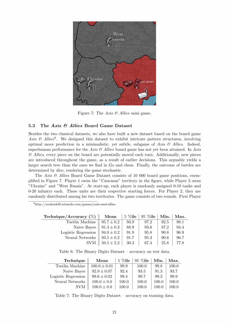
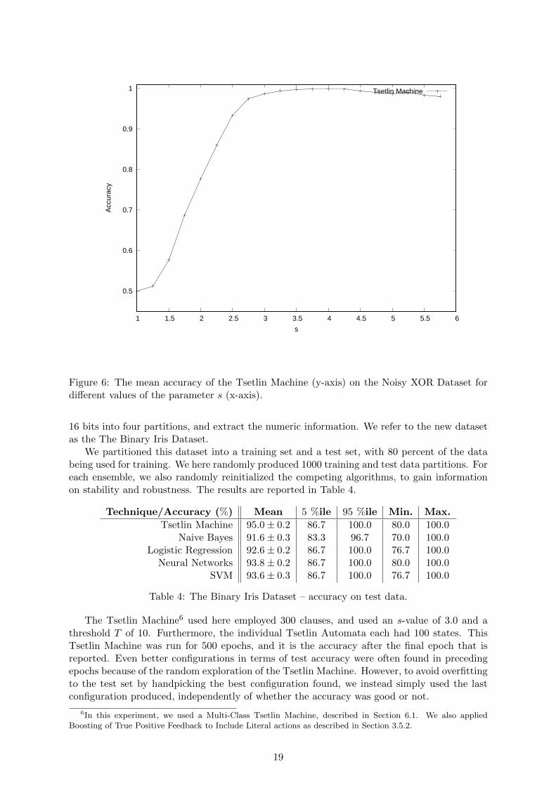
http://archive.ics.uci.edu/ml/datasets/Pen-Based+Recognition+of+Handwritten+Digits

http://archive.ics.uci.edu/ml/datasets/Pen-Based+Recognition+of+Handwritten+Digits

Figure 7: The Axis & Allies mini game.

5.3 The Axis & Allies Board Game Dataset

Besides the two classical datasets, we also have built a new dataset based on the board gameAxis & Allies9. We designed this dataset to exhibit intricate pattern structures, involvingoptimal move prediction in a minimalistic, yet subtle, subgame of Axis & Allies. Indeed,superhuman performance for the Axis & Allies board game has not yet been attained. In Axis& Allies, every piece on the board are potentially moved each turn. Additionally, new piecesare introduced throughout the game, as a result of earlier decisions. This arguably yields alarger search tree than the ones we find in Go and chess. Finally, the outcome of battles aredetermined by dice, rendering the game stochastic.

The Axis & Allies Board Game Dataset consists of 10 000 board game positions, exem-plified in Figure 7. Player 1 owns the ”Caucasus” territory in the figure, while Player 2 owns”Ukraine” and ”West Russia”. At start-up, each player is randomly assigned 0-10 tanks and0-20 infantry each. These units are their respective starting forces. For Player 2, they arerandomly distributed among his two territories. The game consists of two rounds. First Player

9http://avalonhill.wizards.com/games/axis-and-allies




SVM 50.5± 2.2 30.3 67.4 25.8 77.8

Table 6: The Binary Digits Dataset – accuracy on test data.

Technique Mean 5 %ile 95 %ile Min. Max.



SVM 100.0± 0.0 100.0 100.0 100.0 100.0

Table 7: The Binary Digits Dataset – accuracy on training data.

21

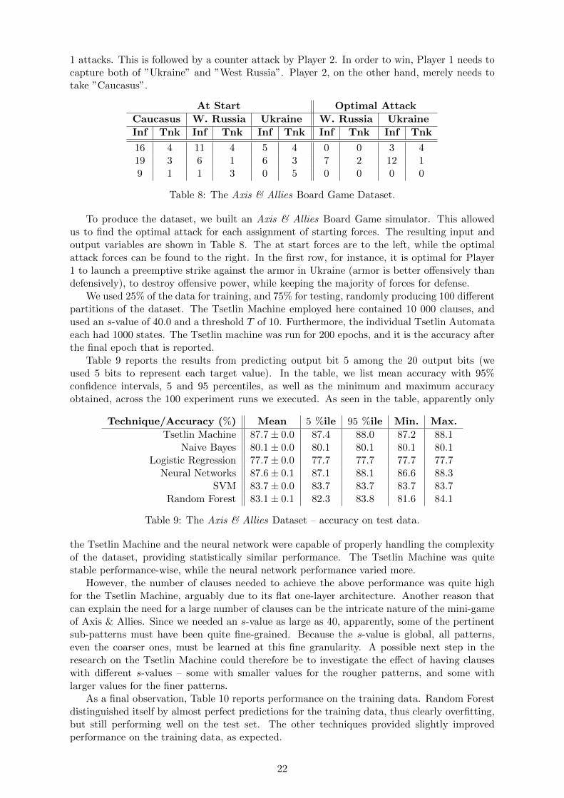
1 attacks. This is followed by a counter attack by Player 2. In order to win, Player 1 needs tocapture both of ”Ukraine” and ”West Russia”. Player 2, on the other hand, merely needs totake ”Caucasus”.

At Start Optimal Attack

Caucasus W. Russia Ukraine W. Russia Ukraine

Inf Tnk Inf Tnk Inf Tnk Inf Tnk Inf Tnk

16 4 11 4 5 4 0 0 3 419 3 6 1 6 3 7 2 12 19 1 1 3 0 5 0 0 0 0

Table 8: The Axis & Allies Board Game Dataset.

To produce the dataset, we built an Axis & Allies Board Game simulator. This allowedus to find the optimal attack for each assignment of starting forces. The resulting input andoutput variables are shown in Table 8. The at start forces are to the left, while the optimalattack forces can be found to the right. In the first row, for instance, it is optimal for Player1 to launch a preemptive strike against the armor in Ukraine (armor is better offensively thandefensively), to destroy offensive power, while keeping the majority of forces for defense.

We used 25% of the data for training, and 75% for testing, randomly producing 100 differentpartitions of the dataset. The Tsetlin Machine employed here contained 10 000 clauses, andused an s-value of 40.0 and a threshold T of 10. Furthermore, the individual Tsetlin Automataeach had 1000 states. The Tsetlin machine was run for 200 epochs, and it is the accuracy afterthe final epoch that is reported.

Table 9 reports the results from predicting output bit 5 among the 20 output bits (weused 5 bits to represent each target value). In the table, we list mean accuracy with 95%confidence intervals, 5 and 95 percentiles, as well as the minimum and maximum accuracyobtained, across the 100 experiment runs we executed. As seen in the table, apparently only




SVM 83.7± 0.0 83.7 83.7 83.7 83.7Random Forest 83.1± 0.1 82.3 83.8 81.6 84.1

Table 9: The Axis & Allies Dataset – accuracy on test data.

the Tsetlin Machine and the neural network were capable of properly handling the complexityof the dataset, providing statistically similar performance. The Tsetlin Machine was quitestable performance-wise, while the neural network performance varied more.

However, the number of clauses needed to achieve the above performance was quite highfor the Tsetlin Machine, arguably due to its flat one-layer architecture. Another reason thatcan explain the need for a large number of clauses can be the intricate nature of the mini-gameof Axis & Allies. Since we needed an s-value as large as 40, apparently, some of the pertinentsub-patterns must have been quite fine-grained. Because the s-value is global, all patterns,even the coarser ones, must be learned at this fine granularity. A possible next step in theresearch on the Tsetlin Machine could therefore be to investigate the effect of having clauseswith different s-values – some with smaller values for the rougher patterns, and some withlarger values for the finer patterns.

As a final observation, Table 10 reports performance on the training data. Random Forestdistinguished itself by almost perfect predictions for the training data, thus clearly overfitting,but still performing well on the test set. The other techniques provided slightly improvedperformance on the training data, as expected.

22

5.4 The Noisy XOR Dataset with Non-informative Features

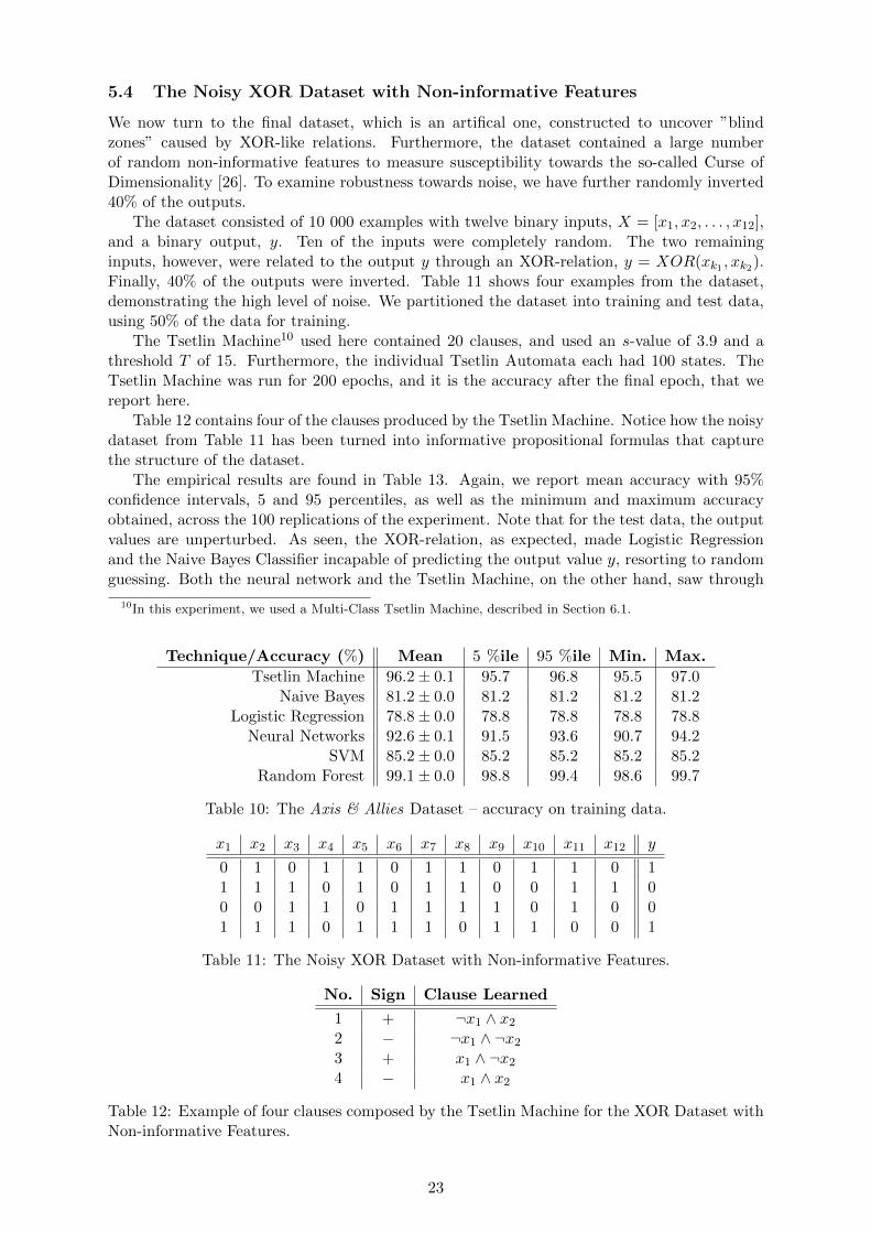
We now turn to the final dataset, which is an artifical one, constructed to uncover ”blindzones” caused by XOR-like relations. Furthermore, the dataset contained a large numberof random non-informative features to measure susceptibility towards the so-called Curse ofDimensionality [26]. To examine robustness towards noise, we have further randomly inverted40% of the outputs.

The dataset consisted of 10 000 examples with twelve binary inputs, X = [x1, x2, . . . , x12],and a binary output, y. Ten of the inputs were completely random. The two remaininginputs, however, were related to the output y through an XOR-relation, y = XOR(xk1 , xk2).Finally, 40% of the outputs were inverted. Table 11 shows four examples from the dataset,demonstrating the high level of noise. We partitioned the dataset into training and test data,using 50% of the data for training.

The Tsetlin Machine10 used here contained 20 clauses, and used an s-value of 3.9 and athreshold T of 15. Furthermore, the individual Tsetlin Automata each had 100 states. TheTsetlin Machine was run for 200 epochs, and it is the accuracy after the final epoch, that wereport here.

Table 12 contains four of the clauses produced by the Tsetlin Machine. Notice how the noisydataset from Table 11 has been turned into informative propositional formulas that capturethe structure of the dataset.

The empirical results are found in Table 13. Again, we report mean accuracy with 95%confidence intervals, 5 and 95 percentiles, as well as the minimum and maximum accuracyobtained, across the 100 replications of the experiment. Note that for the test data, the outputvalues are unperturbed. As seen, the XOR-relation, as expected, made Logistic Regressionand the Naive Bayes Classifier incapable of predicting the output value y, resorting to randomguessing. Both the neural network and the Tsetlin Machine, on the other hand, saw through

10In this experiment, we used a Multi-Class Tsetlin Machine, described in Section 6.1.




SVM 85.2± 0.0 85.2 85.2 85.2 85.2Random Forest 99.1± 0.0 98.8 99.4 98.6 99.7

Table 10: The Axis & Allies Dataset – accuracy on training data.

x1 x2 x3 x4 x5 x6 x7 x8 x9 x10 x11 x12 y

0 1 0 1 1 0 1 1 0 1 1 0 11 1 1 0 1 0 1 1 0 0 1 1 00 0 1 1 0 1 1 1 1 0 1 0 01 1 1 0 1 1 1 0 1 1 0 0 1

Table 11: The Noisy XOR Dataset with Non-informative Features.

No. Sign Clause Learned

1 + ¬x1 ∧ x2

2 − ¬x1 ∧ ¬x2

3 + x1 ∧ ¬x2

4 − x1 ∧ x2

Table 12: Example of four clauses composed by the Tsetlin Machine for the XOR Dataset withNon-informative Features.

23

both the XOR-relationship and the noise, capturing the underlying pattern. SVM performedslightly better than the Naive Bayes Classifier and Logistic Regression, however, was distractedby the random features.




SVM 58.0± 0.3 56.4 59.2 55.4 66.5

Table 13: The Noisy XOR Dataset with Non-informative Features – accuracy on test data.

Figure 8 shows how accuracy degraded with less data, when we varied the dataset size from1000 examples to 20 000 examples. As expected, Naive Bayes and Logistic Regression guessedblindly for all the different data sizes. The main observation, however, is that the accuracyadvantage the Tsetlin Machine had over neural networks increased with less training data.Indeed, it turned out that the Tsetlin Machine performed robustly with small training datasets in all of our experiments.

0.5

0.6

0.7

0.8

0.9

1

0 2000 4000 6000 8000 10000 12000 14000 16000 18000 20000

Accu

racy

# Training Examples

Tsetlin MachineNeural Networks

SVMLogistic Regression

Naive Bayes

Figure 8: Accuracy (y-axis) for the Noisy XOR Dataset for different training dataset sizes(x-axis).

6 The Tsetlin Machine as a Building Block in More AdvancedArchitectures

We have designed the Tsetlin Machine to facilitate building of more advanced architectures. Wewill here present the methodology for connecting multiple Tsetlin Machines in more advancedarchitectures. For demonstration purposes, we will use four different example architectures.

24

6.1 The Multi-Class Tsetlin Machine

In some pattern recognition problems the task is to assign one of n classes to each observedpattern, X. That is, one needs to decide upon a single output value, y ∈ {1, . . . , n}. Such amulti-class pattern recognition problem can be handled by the Tsetlin Machine by representingy as bits, using multiple outputs, yi. In this section, however, we present an alternativearchitecture that addresses the multi-class pattern recognition problem more directly.

… …

…

+ - + -

∑

⌵ ⌵ ⌵ ⌵

0 1 0 … 1 0 1

0/1

∑

0/1

1…n

0/10/1

Selected class

Input

Argmax operator

Summation

ConjunctiveClauses

Argmax

Figure 9: The Multi-Class Tsetlin Machine.

Figure 9 depicts the Multi-Class Tsetlin Machine11 which replaces the threshold function ofeach output yi, i = 1, . . . , n with a single argmax operator. With the argmax operator, theindex i of the largest sum f∑(Ci(X)) is outputted as the final output of the Tsetlin Machine:

y = argmaxi=1,...,n(f∑(Ci(X))). (24)

In this manner, each propositional formula Φi, consisting of clauses Ci, captures the pertinentaspects of the respective class i that it models.

Training is done as described in Section 3.5, apart from one critical modification. Assumewe have y = i for the current observation, (X, y). Then the Tsetlin Automata team behindCi is trained as per yi = 1 in the original Algorithm 1. Additionally, a random class q 6= i isselected. The Tsetlin Automata team behind Cq is then trained in accordance with yi = 0 inthe original algorithm (trained with opposite feedback, i.e., Type I Feedback becomes Type IIFeedback, and vice versa).

6.2 The Fully Connected Deep Tsetlin Machine

Another architectural family is the Fully Connected Deep Tsetlin Machine [27], illustratedin Figure 10. The purpose of this architecture is to build composite propositional formulas,combining the propositional formula composed at one layer into more complex formula at thenext. As exemplified in the figure, we here connect multiple Tsetlin Machines in a sequence.The clause output from each Tsetlin Machine in the sequence is provided as input to thenext Tsetlin Machine in the sequence. In this manner we build a multi-layered system. Forinstance, if layer t produces two clauses (P ∧ ¬Q) and (¬P ∧ Q), layer t + 1 can manipulatethese further, treating them as inputs. Layer t+ 1 could then form more complex formulas like¬(P ∧ ¬Q) ∧ (P ∧ ¬Q), which can be rewritten as (¬P ∨Q) ∧ (P ∧ ¬Q).

One simple approach for training such an architecture is indicated in the figure. As il-lustrated, each layer is trained independently, directly from the output target yi, exactly asdescribed in Section 3.5. The training procedure is thus similar to the strategy Hinton et al.used to train their pioneering Deep Belief Networks, layer-by-layer, in 2006 [28]. Such an ap-proach can be effective when each layer produces abstractions, in the form of clauses, that canbe taken advantage of in the following layer.

11An implementation of the Multi-Class Tsetlin Machine can be found athttps://github.com/cair/TsetlinMachine.

25

… …

…+-

+-

∑

⌵ ⌵ ⌵ ⌵

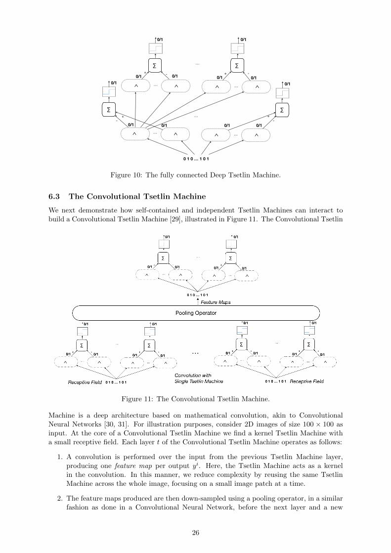
0 1 0 … 1 0 1

0/1

∑

0/1

0/1

0/1

0/1

… …

…

+ - + -∑

⌵ ⌵ ⌵ ⌵

0/1

∑

0/1

0/1

0/10/10/1

0/1

Figure 10: The fully connected Deep Tsetlin Machine.

6.3 The Convolutional Tsetlin Machine

We next demonstrate how self-contained and independent Tsetlin Machines can interact tobuild a Convolutional Tsetlin Machine [29], illustrated in Figure 11. The Convolutional Tsetlin

Figure 11: The Convolutional Tsetlin Machine.

Machine is a deep architecture based on mathematical convolution, akin to ConvolutionalNeural Networks [30, 31]. For illustration purposes, consider 2D images of size 100 × 100 asinput. At the core of a Convolutional Tsetlin Machine we find a kernel Tsetlin Machine witha small receptive field. Each layer t of the Convolutional Tsetlin Machine operates as follows:

1. A convolution is performed over the input from the previous Tsetlin Machine layer,producing one feature map per output yi. Here, the Tsetlin Machine acts as a kernelin the convolution. In this manner, we reduce complexity by reusing the same TsetlinMachine across the whole image, focusing on a small image patch at a time.

2. The feature maps produced are then down-sampled using a pooling operator, in a similarfashion as done in a Convolutional Neural Network, before the next layer and a new

26

Tsetlin Machine takes over. Here, the purpose of the pooling operation is to graduallyincrease the abstraction level of the clauses, layer by layer.

A simple approach for training a Convolutional Tsetlin Machine is indicated in the figure. Inbrief, the feedback to the Tsetlin Machine kernel is directly provided from the desired endoutput yi, exactly as described in Section 3.5. The only difference is the fact that the input tolayer t+ 1 comes from the down-scaled feature map produced by layer t. Again, this is usefulwhen each layer produces abstractions, in the form of clauses, that can be taken advantage ofat the next layer.

6.4 The Recurrent Tsetlin Machine

The final example is the Recurrent Tsetlin Machine [32] (Figure 12). In all brevity, the sameTsetlin Machine is here reused from time step to time step. By taking the output from theclauses of the previous time step as input, together with an external input from the currenttime step, an infinitely deep sequence of Tsetlin Machines is formed. This is quite similar tothe family of Recurrent Neural Networks [33]. Again, the architecture can be trained layer by

Figure 12: The Recurrent Tsetlin Machine.

layer, directly from the target output yi(t) of the current time step t. However, to learn moreadvanced sequential patterns, there is a need for rewarding and penalizing that propagate backin time. How to design such a propagation scheme is presently an open research question.

7 Conclusion and Further Work

In this paper we proposed the Tsetlin Machine, an alternative to neural networks. The TsetlinMachine solves the vanishing signal-to-noise ratio of collectives of Tsetlin Automata. Thisallows it to coordinate thousands of Tsetlin Automata. By equipping teams of Tsetlin Au-tomata with the ability to express patterns in propositional logic, we have enabled them torecognize complex patterns. Furthermore, we proposed a novel decentralized feedback orches-tration mechanism. The mechanism is based on resource allocation principles, with the intentof maximizing effectiveness of sparse pattern recognition capacity. This mechanism effectively

27

provides the Tsetlin Machine with the ability to capture unlabelled sub-patterns. Our theoreti-cal analysis reveals that the Tsetlin Machine forms a set of sub-games where the Nash equilibriamaps to propositional formulas that maximize pattern recognition accuracy. In other words,there are no local optima in the learning process, only global ones. This explains how thecollectives of Tsetlin Automata are able to accurately converge towards complex propositionalformulas that capture the essence of four diverse pattern recognition problems. Overall, theTsetlin Machine is particularly suited for digital computers, being merely based on simple bitmanipulation with AND-, OR-, and NOT gates. Both input, hidden patterns, and outputare expressed with easy-to-interpret bit patterns. In thorough empirical evaluations on fourdistinct benchmarks, the Tsetlin Machine outperformed both single layer neural networks, Sup-port Vector Machines, Random Forests, the Naive Bayes Classifier and Logistic Regression. Itfurther turns out that the Tsetlin Machine requires much less data than neural networks, evenoutperforming the Naive Bayes Classifier in data sparse environments.

The Tsetlin Machine is a completely new tool for machine learning. Based on its solidtheoretical foundation in automata- and game theory, promising empirical results, and itsability to act as a building block in more advanced systems, we believe the Tsetlin Machine hasthe potential to impact the AI field as a whole, opening a wide range of research paths ahead.For instance, by demonstrating that the longstanding problem of vanishing signal-to-noise ratiocan be solved, the Tsetlin Machine provides a new game theoretic framework for recasting theproblem of pattern recognition, which opens opportunities for further advancement. Apart fromthe basic Tsetlin Machine, the Multi-Class Tsetlin Machine, the Fully Connected Deep TsetlinMachine, the Convolution Tsetlin Machine, and the Recurrent Tsetlin Machine architecturescan be an attractive starting point for further exploration. Lastly, the high accuracy androbustness of the Tsetlin Machine, combined with its ability to produce self-contained easy-to-interpret propositional formulas for pattern recognition, makes it attractive for applied research,such as in the safety-critical medical domain.

Code Availability

Source code and datasets for the Tsetlin Machine, available under the MIT Licence, can befound at https://github.com/cair/TsetlinMachine.

Data Availability

The datasets generated during and/or analysed during the current study are available from thecorresponding author on reasonable request.

References

[1] Y. A. LeCun, Y. Bengio, and G. E. Hinton, “Deep learning,” Nature, vol. 521, p. 436–444,2015.

[2] M. L. Tsetlin, “On behaviour of finite automata in random medium,” Avtomat. i Telemekh,vol. 22, no. 10, pp. 1345–1354, 1961.

[3] K. S. Narendra and M. A. L. Thathachar, Learning Automata: An Introduction. Prentice-Hall, Inc., 1989.

[4] J. Carroll, Theory of Finite Automata With an Introduction to Formal Languages. Pren-tice Hall, 1989.

[5] O.-C. Granmo and B. Oommen, “Solving stochastic nonlinear resource allocation prob-lems using a hierarchy of twofold resource allocation automata,” IEEE Transactions onComputers, vol. 59, no. 4, 2010.

28

[6] B. Tung and L. Kleinrock, “Using Finite State Automata to Produce Self-Optimizationand Self-Control,” IEEE Transactions on Parallel and Distributed Systems, vol. 7, no. 4,pp. 47–61, 1996.

[7] O.-C. Granmo, B. J. Oommen, S. A. Myrer, and M. G. Olsen, “Learning Automata-basedSolutions to the Nonlinear Fractional Knapsack Problem with Applications to OptimalResource Allocation,” IEEE Transactions on Systems, Man, and Cybernetics, Part B,vol. 37, no. 1, pp. 166–175, 2007.

[8] B. J. Oommen, “Stochastic Searching on the Line and its Applications to Parameter Learn-ing in Nonlinear Optimization,” IEEE Transactions on Systems, Man, and Cybernetics,Part B, vol. 27, no. 4, pp. 733–739, 1997.

[9] A. Yazidi, O.-C. Granmo, B. John Oommen, and M. Goodwin, “A novel strategy forsolving the stochastic point location problem using a hierarchical searching scheme,” IEEETransactions on Cybernetics, vol. 44, no. 11, pp. 2202 – 2220, 2014.

[10] B. J. Oommen, S.-W. Kim, M. T. Samuel, and O.-C. Granmo, “A solution to the stochasticpoint location problem in metalevel nonstationary environments,” Systems, Man, andCybernetics, Part B: Cybernetics, IEEE Transactions on, vol. 38, no. 2, pp. 466–476,2008.

[11] O.-C. Granmo and N. Bouhmala, “Solving the Satisfiability Problem Using Finite LearningAutomata,” International Journal of Computer Science and Applications, vol. 4, no. 3,pp. 15–29, 2007.

[12] N. Bouhmala and O.-C. Granmo, “Combining Finite Learning Automata with GSAT forthe Satisfiability Problem,” Engineering Applications of Artificial Intelligence (EAAI),vol. 23, no. 5, pp. 715–726, 2010.

[13] ——, “Stochastic Learning for SAT-Encoded Graph Coloring Problems,” InternationalJournal of Applied Metaheuristic Computing, vol. 1, no. 3, pp. 1–19, 2010.

[14] A. Yazidi, O.-C. Granmo, and B. Oommen, “Service selection in stochastic environments:A learning-automaton based solution,” Applied Intelligence, vol. 36, no. 3, pp. 617–637,2012.

[15] V. Haugland, M. Kjølleberg, S.-E. Larsen, and O.-C. Granmo, “A two-armed banditcollective for hierarchical examplar based mining of frequent itemsets with applicationsto intrusion detection,” Transactions on Computational Collective Intelligence XIV, vol.8615, pp. 1–19, 2014.

[16] O.-C. Granmo and B. Oommen, “Optimal sampling for estimation with constrained re-sources using a learning automaton-based solution for the nonlinear fractional knapsackproblem,” Applied Intelligence, vol. 33, no. 1, pp. 3–20, 2010.

[17] A. Yazidi, O.-C. Granmo, and B. Oommen, “Learning-Automaton-Based Online Discov-ery and Tracking of Spatiotemporal Event Patterns,” IEEE Transactions on Cybernetics,vol. 43, no. 3, pp. 1118 – 1130, 2013.

[18] B. J. Oommen and D. C. Y. Ma, “Deterministic learning automata solutions to the equipar-titioning problem,” Computers, IEEE Transactions on, vol. 37, no. 1, pp. 2–13, 1988.

[19] J. Zhang, Y. Wang, C. Wang, and M. Zhou, “Symmetrical Hierarchical Stochastic Search-ing on the Line in Informative and Deceptive Environments,” IEEE Transactions on Cy-bernetics, vol. 47, no. 3, pp. 626 – 635, 7 2016.

29

[20] B. J. Oommen, S. Misra, and O.-C. Granmo, “Routing Bandwidth Guaranteed Paths inMPLS Traffic Engineering: A Multiple Race Track Learning Approach,” IEEE Transac-tions on Computers, vol. 56, no. 7, pp. 959–976, 2007.

[21] M. A. L. Thathachar and P. S. Sastry, Networks of Learning Automata: Techniques forOnline Stochastic Optimization. Kluwer Academic Publishers, 2004.

[22] A. G. Barto and P. Anandan, “Pattern-Recognizing Stochastic Learning Automata,” IEEETransactions on Systems, Man and Cybernetics, vol. 15, no. 3, pp. 360 – 375, 1985.

[23] R. O. Duda, P. E. Hart, and D. G. Stork, “Pattern Classification,” 2001.

[24] T. M. Mitchell, Machine Learning. McGraw-Hill, 1997.

[25] S. A. Cook, “The complexity of theorem-proving procedures,” in Proceedings of the thirdannual ACM symposium on Theory of computing - STOC ’71, 1971.

[26] R. Duda, P. Hart, and D. Stork, Pattern Classification, 2nd ed. New York, NY: JohnWiley and Sons, Inc., 2000.

[27] O.-C. Granmo, “The Recurrent Tsetlin Machine,” In Preparation, 2018.

[28] G. E. Hinton, S. Osindero, and Y.-W. Teh, “A Fast Learning Algorithm for Deep BeliefNets,” Neural Computation, vol. 18, no. 7, pp. 1527 – 1554, 2006.

[29] O.-C. Granmo, “The Convolutional Tsetlin Machine,” In Preparation, 2018.

[30] Y. LeCun, L. Bottou, Y. Bengio, and P. Haffner, “Gradient-based learning applied todocument recognition,” Proceedings of the IEEE, vol. 86, no. 11, pp. 2278 – 2324, 1998.

[31] A. Krizhevsky, I. Sutskever, and G. E. Hinton, “ImageNet Classification with Deep Convo-lutional Neural Networks,” in Proceedings of the 25th International Conference on NeuralInformation Processing Systems, vol. 1, 2012, pp. 1097–1105.

[32] O.-C. Granmo, “The Fully Connected Deep Tsetlin Machine,” In Preparation, 2018.

[33] J. Schmidhuber, “Deep Learning in neural networks: An overview,” Neural Networks,vol. 61, pp. 85–117, 2015.

30

The Tsetlin Machine { A Game Theoretic Bandit Driven Approach to Optimal Pattern Recognition … ·...

Documents

Transcript of The Tsetlin Machine { A Game Theoretic Bandit Driven Approach to Optimal Pattern Recognition … ·...