The tree cover and temperature disparity in US urbanized ...

RESEARCH ARTICLE

The tree cover and temperature disparity in

US urbanized areas: Quantifying the

association with income across 5,723

communities

Robert I. McDonaldID1*, Tanushree Biswas2, Cedilla Sachar3, Ian Housman4, Timothy

M. Boucher5, Deborah Balk6, David Nowak7, Erica Spotswood8, Charlotte K. Stanley2,

Stefan Leyk9,10

1 Center for Sustainability Science, The Nature Conservancy, Arlington, Virginia, United States of America,

2 California Program, The Nature Conservancy, Sacramento, California, United States of America, 3 CUNY

Institute for Demographic Research and CUNY Graduate Center, City University of New York, New York, NY,

United States of America, 4 Independent Researcher, Salt Lake City, Utah, United States of America,

5 Global Science Program, The Nature Conservancy, Arlington, Virginia, United States of America, 6 CUNY

Institute for Demographic Research and Marxe School of International and Public Affairs, Baruch College,

City University of New York, New York, New York, United States of America, 7 Northern Research Station,

USDA Forest Service, Syracuse, New York, United States of America, 8 San Francisco Estuary Institute,

Richmond, California, United States of America, 9 Geography Department, University of Colorado-Boulder,

Boulder, Colorado, United States of America, 10 Institute of Behavioral Science, University of Colorado

Boulder, Boulder, Colorado, United States of America

* [email protected]

Abstract

Urban tree cover provides benefits to human health and well-being, but previous studies

suggest that tree cover is often inequitably distributed. Here, we use National Agriculture

Imagery Program digital ortho photographs to survey the tree cover inequality for Census

blocks in US large urbanized areas, home to 167 million people across 5,723 municipalities

and other Census-designated places. We compared tree cover to summer land surface

temperature, as measured using Landsat imagery. In 92% of the urbanized areas surveyed,

low-income blocks have less tree cover than high-income blocks. On average, low-income

blocks have 15.2% less tree cover and are 1.5˚C hotter than high-income blocks. The great-

est difference between low- and high-income blocks was found in urbanized areas in the

Northeast of the United States, where low-income blocks in some urbanized areas have

30% less tree cover and are 4.0˚C hotter. Even after controlling for population density and

built-up intensity, the positive association between income and tree cover is significant, as is

the positive association between proportion non-Hispanic white and tree cover. We esti-

mate, after controlling for population density, that low-income blocks have 62 million fewer

trees than high-income blocks, equal to a compensatory value of $56 billion ($1,349/per-

son). An investment in tree planting and natural regeneration of $17.6 billion would be

needed to close the tree cover disparity, benefitting 42 million people in low-income blocks.

PLOS ONE

PLOS ONE | https://doi.org/10.1371/journal.pone.0249715 April 28, 2021 1 / 27

a1111111111

a1111111111

a1111111111

a1111111111

a1111111111

OPEN ACCESS

Citation: McDonald RI, Biswas T, Sachar C,

Housman I, Boucher TM, Balk D, et al. (2021) The

tree cover and temperature disparity in US

urbanized areas: Quantifying the association with

income across 5,723 communities. PLoS ONE

16(4): e0249715. https://doi.org/10.1371/journal.

pone.0249715

Editor: Kunwar K. Singh, North Carolina State

University, UNITED STATES

Received: August 5, 2020

Accepted: March 23, 2021

Published: April 28, 2021

Copyright: This is an open access article, free of all

copyright, and may be freely reproduced,

distributed, transmitted, modified, built upon, or

otherwise used by anyone for any lawful purpose.

The work is made available under the Creative

Commons CC0 public domain dedication.

Data Availability Statement: The tree cover data

generated during this study are housed in the KNB

Data Repository (doi:10.5063/MS3R5F). Data can

also be visualized on the GEE platform online. All

code used in data processing is available on GitHub

(https://github.com/tnc-ca-geo/urban-tree-

inequality/blob/main/README.md), or by request

to the corresponding author.

Funding: This work benefitted from support to SL

through NSF’s Humans, Disasters, and the Built

https://orcid.org/0000-0002-7273-6549

https://doi.org/10.1371/journal.pone.0249715

http://crossmark.crossref.org/dialog/?doi=10.1371/journal.pone.0249715&domain=pdf&date_stamp=2021-04-28








https://creativecommons.org/publicdomain/zero/1.0/

https://creativecommons.org/publicdomain/zero/1.0/

https://doi.org/10.5063/MS3R5F

https://github.com/tnc-ca-geo/urban-tree-inequality/blob/main/README.md

https://github.com/tnc-ca-geo/urban-tree-inequality/blob/main/README.md

Introduction

An increasing number of studies, from a variety of disciplines such as ecology, economics, and

environmental health, have found evidence that nature provides multiple benefits to human

health and well-being [1–4]. This paper focuses on one urban natural feature, urban tree can-

opy cover (‘tree cover’ hereafter), the layer of leaves, branches, and stems of woody vegetation

when viewed from above using remote sensing technology [5]. Tree cover provides a variety of

ecosystem service benefits in cities [6, 7], including reducing air pollutant concentrations [8],

mitigating stormwater runoff [7], maintaining water quality [9], encouraging physical recrea-

tion [10], and improving mental health [11]. In the United States, urban trees provide esti-

mated annual benefits of about $18.3 billion in air pollution reduction, carbon sequestration,

and lowered building energy use and power plant emissions [12]. Environmental health scien-

tists have also found epidemiological evidence of a link between trees and human health. A

recent review found that urban trees are associated with a wide range of benefits including:

reduced harms such as ultraviolet radiation, air pollution-related respiratory conditions, and

excess heat stress; greater restorative capacities such as cognition and attention restoration and

benefits to mood and mental health; and positive health effects such as better birth outcomes,

immune functioning, active living, cardiovascular function, weight status, and social cohesion

[4]. Note that urban tree cover is also associated with some ecosystem disservices as well, both

real and perceived [13].

This paper focuses on one benefit tree cover provides, reduced temperatures [8, 14–18].

Urban air temperatures are a function of the urban energy balance, which tree cover and many

other factors influence [19]. Tree cover cools the air primarily by shading surfaces such as con-

crete and asphalt, thus preventing heat storage [19] and reducing the urban heat island effect.

Tree cover can also reduce temperatures by transpiring water, increasing the fraction of heat

going to latent rather than sensible heat [20]. Tree cover can reduce land surface temperature

by 10–20˚C on a summer day [20]. Effects on air temperatures are smaller, with a row of

urban street trees on average lowering summertime air temperatures by 0.5–2.0˚C [21]. This

reduction in air temperature is nevertheless meaningful for human health. One study esti-

mated that current urban tree cover in the United States saves 1200 lives annually during heat-

waves and provides annual heat-reduction services worth $5.3–12.1 billion [22].

Despite the recognition of the numerous benefits provided by tree cover, research suggests

it is unequally distributed in many cities. A meta-analysis of the literature shows that low-

income neighborhoods [23] and minority communities [24] often have less tree cover. These

patterns have been found both within the United States [25] and in other nations [26]. For

instance, Schwarz and colleagues studied 7 incorporated cities and found that neighborhoods

with lower median household income have less tree canopy cover than neighborhoods with

higher income in the same city [27]. Nesbit and colleagues found that across 10 incorporated

cities, neighborhoods with lower education and income had less vegetation, a pattern that was

most strongly apparent in large cities [28]. Riley and Gardiner studied 9 incorporated cities,

examining tree cover and ecosystem service provision, which related to socioeconomic vari-

ables in different ways in each city [29]. A similar general trend for inequality in exposure to

nature has been observed with remotely sensed measures of greenness [30], which have been

used to analyze vegetation in cities globally [e.g., 31], and with exposure to heat risk due to

lack of trees and high impervious cover [32, 33].

Thus, research suggests tree cover is often but not always inequitably distributed in cities,

which may have significant implications for ecosystem service provision and human well-

being [23, 24]. The statistical interpretation of the bivariate negative association between tree

cover and a socio-economic variable like income or race/ethnicity is complex for at least two

PLOS ONE The urban tree cover disparity in US urbanized areas


Environment program (award #1924670 to CU

Boulder) and the Eunice Kennedy Shriver National

Institute of Child Health & Human Development of

the National Institutes of Health under Award

Number P2CHD066613. The results and opinions

expressed in this manuscript are those of the

authors, and do not necessarily represent the views

of any funder or institution supplying data.

Competing interests: The authors have declared

that no competing interests exist.


reasons. First, tree cover is also associated with other factors, including differences in climate,

biome, neighborhood age, urban density, the intensity of urban settlement, and other aspects

of urban form [34–40]. In some studies, covariates such as terrain, housing type and density

explained part of the variation between tree cover and socio-economic variables [25, 29, 39, 41,

42]. Furthermore, socio-economic variables are themselves also correlated with aspects of

urban form, such as the degree of sprawl and population density [43, 44]. Second, some studies

have found that the statistical significance of the relationship between tree cover and socioeco-

nomic variables is different if spatial autocorrelation is accounted for [27, 29], and one review

study observed that studies that controlled for spatial autocorrelation generally found fewer

statistically significant trends [23]. Therefore, one important question when quantifying pat-

terns in tree inequality is whether relationships with socio-economic variables like income and

race/ethnicity are statistically significant after accounting for covariates and spatial

autocorrelation.

Our principal goal for this study is to analyze tree cover and temperature inequality for a

large sample of thousands of communities throughout the United States. To date, however,

such a large survey has been hampered by the lack of fine-resolution data on urban tree cover

with national coverage. For example, the National Land Cover Data (NLCD) Tree Canopy

Cover datasets (2011 and 2016) provide a measure of change in tree cover over five years across

the US but their 30m resolution has been found to systematically underestimate urban tree

cover because small patches of tree canopy are often not detected [45], particularly in land-

scapes below 30% tree cover and above 70% cover [46]. Urban tree canopy (UTC) assessments,

which provide fine-resolution data on tree cover [47], are available in many jurisdictions,

including entire states [e.g., 5, 48]. These UTC assessments are the gold standard for accuracy,

often using local training datasets to create classified tree cover maps from Lidar and high-res-

olution (often < 1m) imagery [e.g., 49–51]. However, UTC assessments are not available for

all communities in the United States, and therefore could not be used to achieve our study’s

goal of analyzing tree cover inequality for a large sample of thousands of communities

throughout the United States.

Here, we analyze the 100 largest urbanized areas in the United States, housing 167 million

people (nearly 55% of the total US population) and containing the urbanized portions of 5,723

incorporated places (cities and towns) and census-designated places in 2010 (see Methods for

definitions of these terms). We focus on tree cover inequality relative to income, hypothesizing

that high-income neighborhoods will have greater urban tree canopy cover. While it is less of a

focus, we also examine tree cover relative to race/ethnicity inequality, hypothesizing that

neighborhoods with a higher proportion of non-Hispanic whites will have greater tree cover.

Key goals of this study include:

• Quantify for a large sample of US communities the degree to which urban tree cover varies

with household income and population density.

• Map for a large sample of US communities the inequality in tree cover and summer tempera-

ture across and within US urbanized areas.

• Test if urban tree cover will be lower in blocks of lower household income even after

accounting for how population density and other covariates that affect the correlation

between income and tree cover.

• Quantify for a large sample of US communities the difference in summer surface tempera-

tures between low and high-income blocks.




• Estimate for a large sample of US communities the US urban tree cover disparity, the

amount of tree planting that would be required to raise low-income blocks up to the median

of similarly dense high-income blocks.

Materials and methods

Our methods proceeded in five stages: defining the study area; remote sensing and image

interpretation; assembling demographic and socioeconomic data; spatial overlay operations in

a geographical information system (GIS) to integrate these data sets; and statistical analysis to

determine significant patterns in tree cover.

Study area

Our study area was all US urbanized areas [52] larger than 500 km2, where “urbanized area”

follows the definition of the US Census for the 2010 census [52]: “an urban area will comprise

a densely settled core of census tracts and/or census blocks that meet minimum population

density requirements, along with adjacent territory containing non-residential urban land uses

as well as territory with low population density included to link outlying densely settled terri-

tory with the densely settled core.” There were 100 urbanized areas larger than 500 km2, with a

population of 167 million people. Note that one urbanized area generally contained multiple

communities: these 100 urbanized areas contained the urbanized portion of 3,520 incorpo-

rated places (e.g., municipalities) and 2,291 census-designated places (places not legally incor-

porated but with commonly used place names that have been mapped by the Census Bureau)

[53].

In this study, tree cover is compared to demographic characteristics derived from US Cen-

sus data available at the block group level (income) or block level (all other demographic and

social variables).

Remote sensing

In order to assess tree cover inequality for a large sample of thousands of communities

throughout the United States, we mapped tree cover at 2m resolution. Our study explored the

application of Google Earth Engine (GEE), a web-based application programming interface

(API) that enables rapid analysis of large spatial datasets [54] to develop a fast, systematic

method to map tree cover across large urbanized areas within the US.

The urbanized areas were grouped into ten geographically defined groups predominantly

determined by their biomes (S1 Table), as defined by Olson and colleagues [55]. The justifica-

tion behind this was that vegetation type, and hence spectral characteristics, are similar within

each biome, allowing optimization of image classification procedures regionally. There were

two exceptions to this assignment of urbanized areas to biome. First, the temperate broadleaf

and mixed forests biome of the eastern United States contains many urbanized areas, and we

decided to split it into subgroups to allow for more locally defined classification algorithms (S1

Fig). Generally, the assignment of urbanized areas in this biome to subgroups followed ecore-

gional boundaries, with adjustments to avoid having a small amount of urbanized area in any

one subgroup. Second, we chose to place western urbanized areas into one group, rather than

assuming urbanized areas in the western United States would be spectrally similar to urban-

ized areas in the eastern United States of the same biome. While that does mean western

urbanized areas span a range of biome types, it allows for the classifier to optimize for the

urban form of cities along the West Coast, which is different than East Coast cities. In practice,

since the random forest algorithm used (see below) is quite flexible, the exact geographical




groupings used in our classification do not appear to affect our results substantially, and pre-

liminary classifications using different geographic groupings yielded qualitatively similar tree

cover maps.

The analysis was based on 2m imagery from the US Department of Agriculture’s National

Agriculture Imagery Program (NAIP) available on Google Earth Engine (GEE). The NAIP

archive between 2014 and 2016 had four spectral bands—blue (B), green (G), red (R), and

near-infrared (NIR) wavelengths—and was filtered for cloud-free images. This time period

was chosen because there was near universal coverage of NAIP images with these four bands,

whereas earlier time periods lack complete coverage. From these four bands, we derived six

additional layers useful for image classification. Three of these were commonly-used indices,

normalized band ratios that are helpful for detecting vegetation and water: Normalized Differ-

ence Vegetation Index (NDVI) [56], Green Normalized Difference Vegetation Index

(GNDVI) [57], and Normalized Difference Water Index (NDWI) [58]. These were defined as:

NDVI ¼ðNIR � RÞðNIRþ RÞ

ð1Þ

GNDVI ¼ðNIR � GÞðNIRþ GÞ

ð2Þ

NDWI ¼ðG � NIRÞðGþ NIRÞ

ð3Þ

To differentiate trees from other green areas such as pasture, baseball fields or golf courses,

we used an entropy function in GEE (image.glcm) that calculated the gray-level co-occurrence

matrix (GLCM) value [59], using as input the NDVI in a 4x4 kernel window. Finally, a binary

layer was created where pixels with high texture value and high NDVI threshold were given a

value of 1, and the remaining pixels were otherwise coded as 0. Thresholds for texture and

NDVI varied by geographic region. Thresholds were chosen to correctly identify forested sites

in the training data as having high NVDI and a high texture value, while avoiding coding areas

of grass as 1. The final ten band image stack (four bands from NAIP imagery, plus six derived

layers) was used in image classification.

Training data for this image classification come from a spatially explicit dataset comprising

of 9,424 control points, created by Nowak and Greenfield [34]. In the Nowak and Greenfield

analysis, each control point in 2014 had a known land cover assigned by a human image inter-

preter looking at aerial photographs. For this analysis, we simplified the Nowak and Greenfield

land cover classes to tree (N = 3746) or not tree (N = 5678). In our analysis, each control point

also has values in each of the ten-band image stack. This information was used to train a Ran-

dom Forests (RF) classification algorithm [60, 61]. The RF classifier in GEE was run separately

for each different geographic area, outputting a classified tree/non-tree image as well as infor-

mation on the confusion matrix and statistics of classification accuracy using the classifier.con-

fusionMatrix function in GEE.

Validation against an independent, high accuracy dataset. Our unit of analysis for this

study was the census block, so we were primarily interested in making sure our tree cover esti-

mates at that scale were accurate. We validated our method for estimating tree cover against

an independent test dataset, some of the Urban Tree Canopy (UTC) assessments conducted

by the US Forest Service. The goal was to validate our methodology against urban tree canopy

assessments that are known to have high accuracy, to ensure our estimates of tree cover at the

census block level are accurate. UTC assessments provide fine-resolution data on urban tree




cover, and typically map forest cover at< 1m resolution, often using Lidar information and

local training datasets [47]. Our mapping effort will not be as accurate at the UTC datasets at

the pixel-level, since we do not have access to such detailed local information for all 5,723 com-

munities in our study area. By validating census-block level tree cover estimates against this

independent, high accuracy data set, we checked to make sure our estimates of forest cover at

the census block level were accurate.

We obtained 34 UTC tree cover layers [5] that were available on the UTC website (http://

gis.w3.uvm.edu/utc/Landcover/) in October 2019 that were contained within our study extent.

Assessed areas range from small municipalities (e.g. Takoma Park, MD) to large counties (e.g.,

Fairfax County, VA), and are primarily in the forested and grassland biomes of the United

States. Note that these are not all the available UTC layers, some of which are available from

different websites and span larger geographies. For our purposes, however, this sample of UTC

layers was sufficient to validate our block level tree cover estimates for forested and grassland

biomes, where the majority of US urban areas lie. We calculated the UTC tree cover in census

blocks (N = 155,916 census blocks) and compared it to our estimates. We tested how well our

tree cover area estimates correlated with the UTC area estimates using simple linear regres-

sion, at the census block level. We also calculated the median absolute error of our block level

estimates of tree cover, compared to that of the UTC estimates.

Demographic/Socioeconomic and built-up intensity data

Based on a review of the literature [23–32], we selected covariates that have been shown in

other studies to be related to urban tree canopy. Covariates also had to be available nationally

at a consistent spatial and temporal scale, as well as applicable in all cities in our study area.

This precluded including some covariates that have been shown to be regionally important but

do not have consistent spatial data over our entire study area (e.g., information on redlined

areas). The covariates we included in our study fit into two broad categories: Demographic

data and information on the fraction of area built up.

Our source for demographic data was primarily the US Decennial Census (2010), down-

loaded from National Historic Geographic Information System (NHGIS) [62]. Our general

strategy was to use the finest spatial resolution demographic data possible, and to conduct our

analysis at this level where possible. We used block level data for population from the US

decennial census, the finest resolution publicly available data. Specifically, we used variable

TotPop in the NHGIS naming system (NHGIS variables names noted hereafter parentheti-

cally). We acknowledge that this predates our tree cover map (2014–2016), and in some areas

with large demographic changes between 2010 and 2014–2016, this may introduce a bias.

However, we chose this approach because we wanted to use the most spatially detailed demo-

graphic data, which is only available for 2010. Moreover, the NAIP imagery in the period

around 2010 was of lesser quality, having fewer spectral bands, so we chose not to try to map

tree cover around 2010.

Total population was divided by the land area (Aland10, available at the census block level)

to calculate the population density within each census block. Our hypothesis was that popula-

tion density would be negatively correlated with tree cover. While we recognize that block

scale population density is not the only attribute describing urban form that is related to tree

canopy cover, several studies have shown evidence of a decay in tree cover as population den-

sity increases [35, 37, 63, 64]. Population density is also an easily accessible metric at broad spa-

tial scales that is both correlated with and related to other aspects of urban form such as

building type, compactness, and average block size [65], and some of these factors have also

been shown to be related to tree cover [35, 36, 42].



http://gis.w3.uvm.edu/utc/Landcover/

http://gis.w3.uvm.edu/utc/Landcover/


Census data on the number of non-Hispanic white residents (NoHiWhite, available at the

census block level) was used to calculate the proportion of residents that were non-Hispanic

white, which we hypothesized would be positively correlated with tree cover. We also included

in our analysis the median age of residents (MedAge, available at the census block level), since

we expected that elderly residents are at greater risk for some diseases, such as negative health

impacts during heat waves.

Per-capita income (IncPr) was taken from the most recent American Community Survey

(ACS) of the Census Bureau (2013–2017 estimates), available at the census block group level.

We used this source of information on income, rather than the 2010 decennial census data, to

have income data that was as close as possible in time to our tree cover imagery (2016). In a

small fraction of cases where block group level estimates were indicated to have low reliability

(having a coefficient of variation larger than 34%), the more reliable tract level estimates were

used [66]. Because block group boundaries of the ACS did not always align with the block

boundaries of the decennial census, we linked to the block-level data using the centroids of the

census blocks. All blocks within the same block group or tract, respectively, shared the same

estimate of income. Our hypothesis was that per-capita income would be positively correlated

with tree cover.

Additionally, we included in our analysis data on the built-up intensity (BUI), a ratio of

indoor floor area of all buildings in a grid cell to the area of that grid cell (250m resolution).

The BUI layer is part of the Historical Settlement Data Compilation of the United States (HIS-

DAC-US) which includes public domain time series of data on the built environment in the

conterminous US derived from Zillow’s ZTRAX database [67]. This information allows us to

account for commercial and industrial areas that may have a small residential population but

large built areas, which we hypothesized would lead to lower levels of tree cover.

Geoprocessing and spatial overlay

Our tree cover maps were overlain in ArcGIS 10.4.1 with the census blocks, to calculate the

tree cover area within each census block using the zonal statistics tool, which calculates sum-

mary statistics within spatial zones (e.g., the census block). Although information from the

census is used to define urbanized areas, the boundaries of the census blocks did not precisely

align with the boundaries of the urbanized areas. Thus, we included in our analysis only those

census blocks whose entire area was inside the urbanized area, buffered out an additional

100m. This small buffer zone accounted for slight non-alignment of census block boundaries

with the urbanized area boundaries. We also excluded from further calculations census blocks

with no people in them. When making maps, we used base layers from the Natural Earth data

library (https://www.naturalearthdata.com/).

Surface temperature. We were interested in having another response variable. We chose

to examine land surface temperature (hereafter “surface temperature”), which is easily quanti-

fiable from satellite imagery. High-resolution information on surface temperature was not

available for the thousands of communities examined in this study. We chose to use Landsat-

derived surface temperature, which is at 30m resolution. The unit of statistical analysis for our

study (see below) was the census block, and there were multiple Landsat pixels within census

blocks.

Median summer surface temperature for images between June 21—September 22 from

2000 to 2019 was calculated using Landsat thermal data. We chose to use this 20-year median

summer surface temperature to average over the high temporal variability in surface tempera-

tures, because exploratory analyses with shorter time intervals yielded spatially variable results

based upon individual seasonal weather events. While a shorter time interval centered around



https://www.naturalearthdata.com/


2016 (our date for tree cover mapping) would potentially allow for a more temporally accurate

estimation of surface temperature for 30m pixels that experienced a land use or land cover

change from 2000–2019, we found that shorter time intervals decreased the precision in our

estimates of surface temperature and obscured spatial patterns in surface temperature.

Landsat 5 and Landsat 8 Thermal Infrared Sensor (TIRS) data within the Tier 1 Surface

Reflectance collections [68] were accessed through Google Earth Engine [54]. Landsat 5 B6

and Landsat 8 B10 provides surface temperature in degrees Kelvin. In order to avoid contami-

nation by clouds and cloud shadows, masking was performed using the pre-computed quality

assurance bands that are part of the Tier 1 products. These masks were created using the

cFmask algorithm [69]. Any pixel identified as bit 5 (cloud) or 2 (cloud shadow) within the

"pixel_qa" band was omitted from the analysis. The final median summer temperature was cal-

culated from the remaining values. Temperature data over surface water was masked out using

the European Commission, Joint Research Centre’s version 1.1 2016 yearly historical surface

water product [70]. Any area identified as permanent or seasonal water was omitted from the

analysis. For more details on our surface temperature analysis, please see our code in GitHub

(see Acknowledgements).

Statistical analysis

Our statistical analysis proceeded in four steps. First, we conducted descriptive analyses, focus-

ing on the spatial patterns of tree cover and temperature inequality, as well as the bivariate rela-

tionship of these variables with income. Second, we conducted a statistical analysis of trends

among urbanized areas, after accounting for the effect of covariates and spatial autocorrela-

tion. Third, we conducted a statistical analysis of trends within urbanized areas, after account-

ing for the effect of covariates and spatial autocorrelation. Finally, we calculated the tree

disparity with respect to income, using information on this bivariate relationship to estimate

the number of trees that would have to be planted to bring tree cover in low-income neighbor-

hoods up to the level of tree cover in equivalently dense high-income neighborhoods.

Descriptive analysis. The unit of analysis for our study was the census block. Census

blocks are the smallest geographic unit for which demographic data is available from the US

Census Bureau, and in cities often correspond to individual city blocks bounded by streets. By

using this fine spatial grain, our analysis focused in on the tree cover near people’s homes.

Tree cover near homes is important since most studies of the impact of nature on human

health find statistical associations most frequently when the greenness is within a few hundred

meters of people’s homes. For instance, James and colleagues found a 12% lower all-cause

mortality rate for women with more greenness within 250m of their home [71].

We divided census blocks into quartiles by per-capita income, defined within an urbanized

area. This allowed the thresholds for being in a particular income quartile to vary by urbanized

area, accounting for the large differences in income among urbanized areas of the United

States. We divided census blocks into four groups by population density, using consistent

ranges of population density for all urbanized areas (0–2000 people/km2, 2000–4000 people/

km2, 4000–8000 people/km2, and> 8000 people/km2). These ranges were chosen to approxi-

mately divide census blocks in our study area into evenly sized groups, but with rounded

break points that were easily understood. We then calculated the population-weighted median

tree cover (%), by income and population density category, within each urbanized area. The

population-weighted median was chosen for our analysis because our analysis focus was the

average tree cover experienced by people near their home, which is what has been found rele-

vant for human well-being and health [22]. Note that for many cities, most tree cover is in

large parks where few or no people live, and most people live in neighborhoods with relatively




little tree cover. In this situation, the population-weighted median is less than the mean tree

cover across the entire city.

Examination of the distribution of proportion non-Hispanic white showed a distinctive

bimodal distribution (i.e., most blocks are predominately white or predominately non-white,

with relatively few blocks in between). Accordingly, we created a binary categorical variable,

which is coded as 1 if the block is majority non-Hispanic white and 0 otherwise.

Analysis among urbanized areas. For this analysis, the unit of analysis is the urbanized

area (N = 100). We conducted two regressions of patterns among urbanized areas. The first

regression predicted median tree cover at the urbanized area level. The second regression pre-

dicted the difference in median tree cover between income quartiles (top quartile minus bot-

tom quartile). Potential explanatory variables considered were all measured at the urbanized

area level, and included: median per-capita income, variation (interquartile range) of per-cap-

ita income, median population density, variation (interquartile range) of population density,

and biome (a categorical variable that describes major climate and ecological gradients [55]).

Population density was log transformed to improve normality. Tree cover was arcsine-

transformed to improve normality. Arcsine transformation is a common transformation of

ecological proportion data [72]. While it has been occasionally criticized as less interpretable

for proportion data than the logit transformation [73], we chose to use it because tree cover

often has extreme values (0’s or 1’s) that are undefined for the logit transformation but are

defined for the arcsine transformation. Forward selection using AIC was used to select the var-

iables to be included in our two regressions.

Analysis of variograms of model residuals suggested moderate spatial autocorrelation

between urbanized areas closer than 500km, and the spatial autocorrelation was found to be

statistically significant using Moran’s I for both regressions (P< 0.05). Accordingly, we tested

for the appropriate model structure using the Lagrange Multiplier Tests, using the lm.morant-

est function in the spdep library in R [74]. Results indicated a spatial lag SAR model was most

appropriate for both regressions, which we used for all among urbanized area regression

results reported in this manuscript.

Analysis within urbanized areas. For this second statistical analysis, each urbanized area

was analyzed separately. The unit of analysis is the census block (N = 1,938,386 total across all

urbanized areas). As census blocks are contiguous with one another, and tree cover was highly

spatially autocorrelated, it was necessary to account for any potential spatial autocorrelation.

Tree cover was arcsine transformed to improve normality. The explanatory variables used in

this within urbanized areas analysis were population density category, income quartile, BUI

category, income category, and majority non-Hispanic white status. These variables were cho-

sen for inclusion in the regression because they were correlated to the response variable and

were only moderately colinear with one another, reducing problems with multicollinearity

during parameter estimation and significance testing. To test for spatial autocorrelation, we

first ran a simple linear regression that predicted tree cover from our explanatory variables

(Proc Mixed in SAS 9.4), and then analyzed the spatial autocorrelation in the residuals (Proc

Variogram), by urbanized area. Spatial autocorrelation was always significant at scales less

than 1km, and for some urbanized areas was significant out to scales of 2km. To address this

spatial autocorrelation and appropriately account for it in our estimation of regression param-

eters, we conducted a block bootstrap [75] using the R package ‘sperrorest’ [76]. Block boot-

straps of 2km were drawn from each urbanized area 1000 times, and for each bootstrap a

regression was calculated. The distribution of bootstrapped parameters was approximately

normal, and we assessed a parameter statistically significant within an urbanized area if at least

95% of the time its value was different than zero.




Tree disparity with respect to income. One of the goals of this research paper was to esti-

mate the US urban tree cover disparity, which we defined as the amount of tree planting that

would be required to raise low-income blocks up to the median level of tree cover in high-

income blocks in the same population density category. The intent in this calculation was not

to statistically model the impact of all covariates (e.g., race/ethnicity, age, BUI), which we did

in a different analysis step (see subsection “Analysis within urbanized area”). Rather, our intent

was to provide a descriptive, policy-relevant measure of the disparity between low- and high-

income blocks of similar urban form. We acknowledge that this is a hypothetical calculation of

the amount of trees that would be required to close this urban tree cover disparity, and that it

may not be feasible or desirable to entirely close this disparity, given competing land-uses and

community preferences in some locations.

In order to calculate tree disparity, for each urbanized area we took the estimates of tree

cover (%) in each population density and income category, and converted these estimates to

the difference in tree cover area by multiplying by the area of the census block. We then esti-

mated the number of adult trees required to fill this tree cover area, using a factor of 19.6 m2 of

canopy cover per urban tree, which was derived from Nowak and Greenfield [12], who esti-

mated that there were 5.5 billion urban trees in 2010 over 67.6 million acres of urban area that

is on average 39.3% tree cover. To estimate the cost of planting new saplings to close the tree

cover disparity, we used a factor of $283/stem, which was derived from the review of tree plant-

ing costs in multiple US cities by Krueger et al. [8]. To estimate the lost value to people repre-

sented by the current US urban tree cover disparity, we calculated the compensatory value,

using the average value per stem reported by Nowak [77]. Compensatory value is one way to

estimate the total value of a tree and represents what compensation should be paid to the tree’s

owner if the tree is lost [77]. While we acknowledge there are other ways to value the benefits

provided by trees [78], we included the compensatory value in our analysis to show that differ-

ences in tree cover between low- and high-income blocks amounted to a substantial difference

in the financial value of this amenity available.

Results

Tree cover classification algorithm

Our classification method successfully mapped tree cover in the 100 largest urbanized areas in

the United States (Fig 1), which cover a total area of 158,000 km2 or 39.6 billion pixels at 2m

spatial resolution. To document the results of the random forest algorithm, pixel-level classifi-

cation accuracy is shown in S1 Table, but note that we did not use pixel-level data in our analy-

sis of tree cover disparities, but instead used aggregated results at the census block level. Pixel-

level classification accuracy was greatest in forested biomes and lower accuracy in biomes like

deserts and grasslands. Across all urbanized areas, average user’s accuracy of the forest class

was 82.1%. The average kappa statistic was 0.45, which would be rated by Landis and Koch

[79] as moderate accuracy. The kappa statistic is widely used in remote sensing, but see citation

[80] for a discussion of its limitations.

Tree cover validation against an independent dataset

Our unit of analysis for this paper was the census block level, and it was thus our goal to consis-

tently map tree cover accurately at the census block level. Census blocks contain many 2m pix-

els, and if classification errors are relatively spatially uncorrelated then the estimate of tree

cover at the census block level can be more accurate than at the pixel-level scale. To assess the

accuracy of our forest cover estimates at the block level, we validated our estimates of tree

cover at the census block level against an independent dataset, the accurate high-resolution




tree cover maps produced by Urban Tree Canopy (UTC) assessments [47]. At the block level,

our estimates of tree cover were highly linearly correlated with those of the UTCs (R = 0.97, S2

Fig). On average, the median absolute block-level error of our tree cover estimate, as compared

against the gold standard estimates of the UTCs, was 6.0%. Thus, while the pixel-level accuracy

of our classification was only moderate, our estimates of tree cover at the block-level were

highly correlated with an independent validation dataset.

In much of our analysis of tree cover disparities, we analyzed aggregated information on

tree cover relative to income, looking across many urbanized areas to come up with national

estimates. To assess our accuracy at this scale, we calculated an estimate of median tree cover

by income category across the entire validation dataset, using both our tree cover datasets and

the UTC dataset. Median errors were small in income quartiles 1 (2.8%), 2 (3.4%), and income

quartile 3 (3.0%) but were slightly larger in income quartile 4 (5.7%). In all income quartiles,

the estimate of tree cover was slightly greater in the UTC dataset than in our tree cover dataset.

Overall median error for the whole validation dataset was 3.6%.

Tree cover, income and population density

Income was inversely associated with tree cover (Fig 2). On average, an increase in relative

income of 5% (for example, from the 15th to the 20th percentile) increases tree cover by 1.2%.

The relationship between tree cover and relative income appears to be approximately linear.

Within each urbanized area, we divided the census blocks into quartiles based upon the per-

capita income distribution. Averaging across all urbanized areas, the least affluent quartile of

census blocks had a median tree cover of 19.7%, while the most affluent quartile had a median

Fig 1. Urbanized areas mapped in this study. Tree cover was mapped for 2016. An inset map of the tree cover (green) of a portion of

the Los Angeles urbanized area is shown. Within the area mapped in the inset, there were 93 municipalities and 34 census-designated

places, whose outlines are shown with black lines.

https://doi.org/10.1371/journal.pone.0249715.g001





tree cover of 34.9% (Table 1). Clearly, low- and high-income blocks nationwide had very dif-

ferent levels of tree cover, and thus likely different levels of ecosystem service (or disservice)

provision.

The relationship between income and tree cover was partially explained by population den-

sity (Table 1). Population density is of course only one aspect of urban form that could affect

urban tree canopy distribution but is a commonly measured summary statistic that we exam-

ined relative to tree cover. In the census blocks in the least affluent quartile, the majority (56%)

of the population lived in blocks in the high (4000–8000 people/km2) or highest population

density (>8000 people/km2) categories, typified by multi-unit buildings. In contrast, in the

census blocks in the most affluent quartile, the majority (55%) of the population lived in blocks

in the lowest (< 2000 people/km2) population density category, typified by single family

Fig 2. Tree cover as a function of income. We classified census blocks based upon the income distribution within its

urbanized area, calculating the percentile of the income distribution that block has. For ease of display, blocks were

grouped into income categories (0–5%, 5–10%, etc.) and the population-weighted median tree cover (%) across the

entire study area calculated. This paper focuses most of its analysis on the lowest quartile (red squares) and highest

quartile (green triangles) of income.


Table 1. Median tree cover, by population density and income categories.

Percent Tree cover Population in category, millions Area in category, km2

Population density (people/km2) Low-income High-income Low-income High-income Low-income High-income

Very low (<2000) 40.0% 47.5% 8.1 23.0 12,528 40,220

Low (2000–4000) 26.7% 28.8% 10.4 10.3 3,656 3,853

Moderate (4000–8000) 17.6% 19.5% 9.9 3.6 1,816 691

High (>8000) 11.4% 10.5% 13.3 4.6 905 271

Across all blocks 19.7% 34.9% 41.7 41.5 18,906 45,035

Tree cover was compared between low and high-income quartiles, over 5,723 incorporated towns and other places in the US. Statistical significance of these trends is

discussed in the section of the manuscript entitled “Evaluating Statistical Significance.”

https://doi.org/10.1371/journal.pone.0249715.t001






homes on large lots. Tree cover was inversely associated with population density (Table 1), pre-

sumably because there was simply less area to fit trees into the landscape when a large fraction

of the area is devoted to buildings and impervious surfaces. However, even when stratifying by

population density, income of a census block was still associated with tree cover. In most popu-

lation density categories, tree cover was greater in the most affluent income quartile than in

the least affluent. Interestingly, the difference in tree cover between low- and high-income cen-

sus blocks was greatest in the lowest population density category, and less in the high or high-

est population density categories. In other words, inequality in tree cover appeared greater in

the exurbs and far suburbs—areas with greater potentially vegetated area—than in denser

blocks.

Patterns across the United States

Patterns in tree cover across US urbanized areas are shown in Fig 3. Median tree cover (Fig 3A)

was greatest in urbanized areas in the South like Atlanta and lowest in urbanized areas in the

Southwest like Phoenix. Much of this regional pattern in median tree cover was explained by

biome, with urbanized areas in forested biomes having more tree cover than those in other

biomes such as desert or grassland (urbanized area level regression, S2 Table, P = 0.005). This pat-

tern has been found in other studies as well [12], and is expected as tree cover is the natural state

in forested biomes, as opposed to being intentionally planted in other biomes. Another important

variable in explaining variation in tree cover was population density, with urbanized areas with

higher median population density (e.g., urbanized areas in the Northeast such as New York City

and Philadelphia) having lower tree cover, presumably because there was simply less area to fit

trees into more densely developed areas (P = 0.0002). After accounting for these other variables,

median per-capita income in an urbanized area was not a significant predictor of median tree

cover in that urbanized area (P = 0.41). Median tree cover for all 5,723 incorporated places (cities

and towns) and census-designated places surveyed in this paper can be found in S3 Table.

We quantified for each urbanized area the difference in tree cover between low and high-

income blocks (Fig 3B). We found that a trend toward greater tree cover in high-income

blocks occurred in 92% of the urbanized areas we examined (S4 Table). The greatest difference

in tree cover between low- and high-income blocks was found in urbanized areas in the North-

east of the United States, particularly along the coast between Washington, DC and Boston,

MA (Fig 3B). The urbanized area with the greatest difference in tree cover between low- and

high-income blocks was the Stamford/Bridgeport, CT area (54%). Conversely, the West and

Southwest had generally smaller differences in tree cover between low- and high-income

blocks, likely because of the generally lower tree cover in those biomes. In a few urbanized

areas, primarily in the South (e.g., Cape Coral, FL, Jackson MS), median tree cover was greater

in low-income blocks than in high income areas (see Discussion section for description of why

this trend may have occurred).

The strongest predictor of the difference in tree cover between high- and low-income

blocks was income inequality (urbanized area level regression, S2 Table, P < 0.0001). Urban-

ized areas with greater income inequality (as measured by the interquartile range) had greater

differences in tree cover between high- and low-income blocks. Urbanized areas with a greater

range of population densities (as measured by the interquartile range) had greater differences

in tree cover between high- and low-income blocks (P = 0.0006). Finally, urbanized areas with

a greater median tree cover had smaller differences in tree cover between high- and low-

income blocks (P = 0.005). After accounting for these other variables, biome was not a statisti-

cally significant predictor of the difference in tree cover between high- and low-income blocks

(P = 0.77).




Fig 3. Tree cover for United States large urbanized areas. a.) Population-weighted median tree cover. b.) The absolute difference

between low-income blocks (lowest quartile of income) and high-income blocks (highest quartile of income) in tree cover.






Patterns within urbanized areas

Patterns for individual cities can be visualized online. Generally, the highest population densi-

ties can be found in the center of an urbanized area [c.f., 81], with average income and average

tree cover that were lower than the averages for the entire urbanized area. More suburban or

exurban areas, often in separate municipalities or census-designated places, had lower popula-

tion density, higher average income, and higher average tree cover. In other words, the spatial

transition from suburban to urban core related to a gradient in both tree cover and income, a

pattern that can be expected for many US urbanized areas [82]. Many other variables corre-

lated with income and thus show similar associations with tree cover (Fig 4). More affluent

census blocks had a greater proportion of non-Hispanic whites and generally had more tree

cover. In contrast, blocks with a lower proportion of non-Hispanic whites generally had less

tree cover. Residents of more affluent blocks also tended to be older than residents of less afflu-

ent blocks, and the median age of residents was positively associated with tree cover.

Evaluating statistical significance

We assessed for each city separately whether income or race were significantly related to tree

cover, after accounting for covariates (population density, income, built-up intensity, and

race/ethnicity) and spatial autocorrelation using a block bootstrap approach. This block boot-

strap approach allows an estimate of the confidence interval of regression parameter after

accounting for the spatial autocorrelation, with a parameter considered significant if they are

statistically different than zero.

Fig 4. Patterns across blocks of different incomes. Census blocks within each urbanized area were classified by the

quartile of income they occupy. For each quartile, we show the median tree cover, population density, age, and percent

non-Hispanic white.






Population density was the covariate most commonly statistically significant in our regres-

sions (S5 Table), with the highest population density category having significantly less tree

cover than the lowest population density category in 94 urbanized areas. Income was the sec-

ond most common statistically significant effect (S5 Table), with the highest income category

having significantly more tree cover than the lowest income category in 78 urbanized areas.

Similarly, majority non-Hispanic white blocks had significantly more tree cover than did

majority non-white blocks in 67 urbanized areas. Finally, we included in our statistical analysis

the built up intensity (BUI), a ratio of indoor floor area of all buildings in an area to the land

area. BUI was negatively related to tree cover and was statistically significant in 68 urbanized

area.

From our statistical analysis, we concluded that even after accounting for spatial autocorre-

lation among census blocks and covariates like population density and BUI, income and race/

ethnicity had statistically significant relationships with tree cover in 78% and 67% of the

urbanized areas, respectively.

Surface temperature differences

Not surprisingly, summer surface temperatures were highest in cities in arid biomes in the

western United States (Fig 5A). Averaged across our study area, the least affluent quartile of

census blocks had a summer surface temperature that was 1.5˚C hotter than the most affluent

quartile of census blocks. The variation among urbanized areas was large, however, with the

greatest difference in summer surface temperature between low- and high-income blocks

being 5.4˚C in the Providence urbanized area (Fig 5B, S4 Table). The difference in summer

surface temperature between low- and high-income blocks was highly correlated to the tree

cover difference (R = 0.82, S3 Fig). The greatest differences in summer surface temperature

between low- and high-income blocks were in the Northeast, where, in addition to Providence,

three other urbanized areas had differences of more than 4.0˚C: Bridgeport/Stamford, Worces-

ter, and Philadelphia. Another 9 urbanized areas, including Boston, had differences greater

than 3.0˚C but less than 4.0˚C.

Tree cover disparity

Since tree cover was correlated with population density differences, we chose to examine the

difference in tree cover between low- and high-income blocks after accounting for population

density difference. Within a given population density category, we calculated the disparity in

tree cover between low- and high-income blocks (Table 2). Across all urbanized areas, 1,217

km2 of new tree cover would hypothetically be needed. S6 Table shows these numbers broken

down by urbanized area and population density category. The Seattle urbanized area had the

largest disparity in tree cover in areal terms (74 km2), followed by the Chicago (54 km2) and

Detroit (54 km2) urbanized areas.

We estimated that the least affluent quartile of blocks had 62 million fewer trees in it than

the most affluent quartile (Table 2). This tree cover disparity, even after controlling for popula-

tion density, meant low-income blocks had $56 billion (range: $41–113 billion) less in com-

pensatory value. This is an average of $1,349/person less in compensatory value.

We estimated the cost of tree planting of saplings and their maintenance to close the urban

tree cover disparity (Table 2). In total, approximately $18 billion in tree planting would be

needed to close this tree cover disparity. Note that this figure was less than the compensatory

value, because trees are assets that appreciate over time; after planting a tree sapling increases

in compensatory value as it grows. Note also that our estimate assumed that all new trees are

planted, but there is potential that land-use changes (e.g., stopping mowing) could allow for




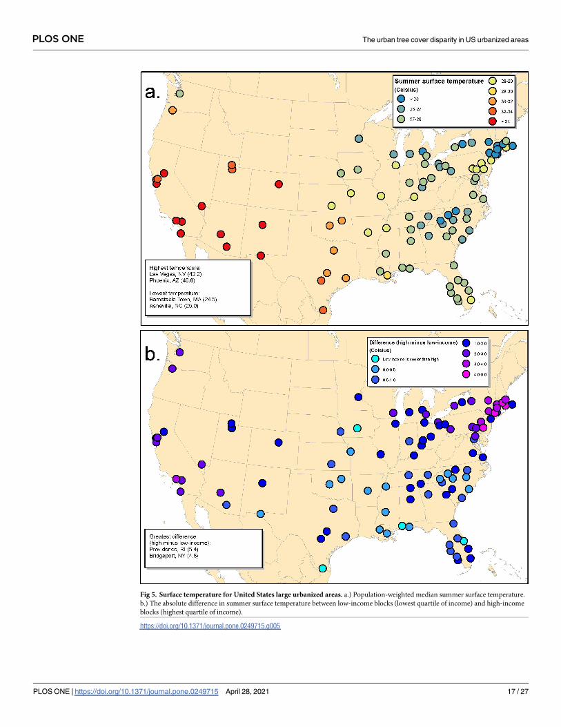
Fig 5. Surface temperature for United States large urbanized areas. a.) Population-weighted median summer surface temperature.

b.) The absolute difference in summer surface temperature between low-income blocks (lowest quartile of income) and high-income

blocks (highest quartile of income).






increased natural regeneration. Because natural regeneration is often free or very low cost, that

would be a more economical way to increase urban tree canopy on some sites.

The vast majority of needed adult trees to close the tree cover disparity would be in the

Very Low population density category (Table 2). This happened because low-income blocks in

the Very Low population density category covered a large area (12,528 km2) and there was a

large difference in tree cover between low-income and high-income blocks (9.8%), leading to

an estimated 50 million trees needed to close the tree cover disparity in this population density

category. However, relatively few people lived in low-income blocks in the Very Low popula-

tion density category. Potentially, for biomes that allow natural forest regeneration, land-use

management strategies that encourage natural regeneration may be more economical for this

category than tree planting.

Discussion

Our research shows that inequality in tree cover between low- and high-income blocks was

widespread in the US, occurring in 92% of the urbanized areas we studied (N = 5,723 cities

and other places). On average, there were 15.2% more tree cover in high-income blocks than

in low-income blocks (Table 1). Our results are consistent with other studies [23–32] that

show tree cover inequality relative to income for many but not all cities.

The Stamford/Bridgeport, CT area had the greatest difference in tree cover between low-

and high-income blocks (54%). This example illustrates why it may be insightful to analyze

inequality in tree cover across an urbanized area, in addition to analyzing trends within spe-

cific municipalities. Stamford and Bridgeport are considered one urbanized area by the US

Census Bureau, and workers commonly commute between them. However, the two munici-

palities have very different histories. Bridgeport developed as an industrial town, where work-

ers lived in densely populated areas near factories [83]; in the 1970s and 1980s the economy

suffered as the industrial sector declined. In contrast, Stamford developed at least in part as a

place for summer vacation homes for New York City residents [84], and currently is economi-

cally well-off. Today, Bridgeport’s tree cover is 20.2% and Stamford’s is 37.1%. While there are

differences in tree cover within each of these two municipalities, much of the difference in tree

cover between low- and high-income blocks in the entire urbanized area comes from

Table 2. The tree cover disparity.

Population density category (people/km2)

Very Low(<2000)

Low (2000–4000)

Medium (4000–8000)

High (>8000) Total across all population density

classes

Total area (km2) of low-income census blocks 12,528 3,656 1,816 905 18,906

Total population of low-income census blocks 8,120,985 10,431,696 9,863,540 13,326,870 41,743,091

Tree cover disparity (%) 9.8% 3.7% 2.6% 3.3% 4.9%

Needed tree cover to close disparity (km2) 985 171 50 11 1,217

Trees required to close disparity 50,367,030 8,762,004 2,547,062 575,105 62,251,201

Compensatory value, billions (median) $45.5 $7.9 $2.3 $0.5 $56.3

Compensatory value, billions (low) $32.9 $5.7 $1.7 $0.4 $40.7

Compensatory value, billions (high) $91.3 $15.9 $4.6 $1.0 $112.8

Cost of planting new saplings to close disparity,

billions

$14.3 $2.5 $0.7 $0.2 $17.6

Shown is the tree disparity between low- and high-income categories after accounting for population density. Compensatory values shown are the disparity in tree cover

value in low- and high-income categories, in billions of USD2019. Compensatory value is the compensation to owners for loss of a tree and can be viewed as one way to

value the tree as an asset.






differences between these two municipalities. Overall, our results suggest that prior studies

that examined tree cover within particular municipalities [e.g., 27, 28, 33] may find a smaller

difference in tree cover between low-income and high income blocks than would exist across

an entire urbanized area, because US urbanized areas are subdivided into jurisdictions that

often have different income distributions.

For the 100 urbanized areas we studied, we found that inequality in tree cover was corre-

lated with differences in the average population density found in low- and high-income blocks,

consistent with other studies in the literature that have discussed demographic patterns relative

to tree cover patterns [85, 86]. As in other studies [e.g., 23, 27, 29], accounting for covariates

and spatial autocorrelation reduced the strength of the association between income and tree

cover, but income was still significantly associated with tree cover in 78% of the urbanized

areas studied. Note that while population density was negatively correlated with tree cover,

this correlation was not perfect, and at any given population density class there were blocks

that have relatively high tree cover and others with relatively low tree cover. Accordingly, it

was possible to find dense blocks that still had relatively high tree cover.

Note that there were 22% of urbanized areas where there was not a statistically significant

relationship between income and tree cover. Eight percent of the 100 urbanized areas studied

had median tree cover that was actually greater in low-income blocks than in high income

areas. This occurred in urbanized areas with many blocks, both low-income and high-income,

in the Very Low population density category. It is possible that there was still variation in pop-

ulation density within this Very Low population density category. For instance, in the Cape

Coral urbanized area, there were many blocks in the Very Low population density category in

both Naples (a relatively affluent community near the coast) and Lehigh Acres (a less affluent

community more inland), but the latter had relatively greater tree cover and lower population

density, presumably because the lower population density allowed larger lot sizes that are

more forested. Another 14% of the 100 urbanized areas studied had tree cover that was greater

in high-income areas than in low-income areas, but the trend was fully explained after

accounting for covariates and spatial autocorrelation. These urbanized areas also tended to

have most of their blocks in the Very Low population density category. For instance, Houston,

a very low population density city, had 8.1% more tree cover in high-income than in low-

income neighborhoods (S4 Table) but this trend was not statistically significant after account-

ing for covariates and spatial autocorrelation (S5 Table).

There are two main potential causes of this pervasive inequality in tree cover between low-

and high-income blocks. First, differences among blocks in tree cover in the public right of

way along roads and in other publicly owned land could be due to differential investments by

municipal or local governments. Commonly, in the urban core with high-density blocks, a

greater fraction of the land area is in public ownership, either as parks [87] or as part of the

road right of way [88], as compared to lower density blocks in the suburbs or in rural areas.

Thus, tree cover in dense blocks is particularly shaped by the actions of municipal govern-

ments. The fragmentation of US urbanized areas into many different municipalities [89], with

different levels of economic development and hence different levels of potential government

spending [90], worsens inequality in tree cover at the scale of the entire urbanized area. Low-

income households are often clustered in low-income municipalities that have fewer resources

to plant and maintain trees on public land, and so these municipalities could end up with

fewer trees than their high-income counterparts. Even within one municipality, there can be

differential public-sector investment in trees in low-income neighborhoods [91]. Sometimes

low-income households may be less likely to participate in voluntary tree planting programs

[92]. Historically, there have also been instances of explicit racism in urban planning and zon-

ing decisions, such as the practice of redlining (refusing home loans or insurance to specific,




generally minority, neighborhoods). Studies have showed that areas that were redlined have

higher surface temperature [93–95], presumably in part because they have lower tree cover.

Second, differences among census blocks in tree cover on privately-owned land could be

because of differential land-use decisions by private landowners, as well as differential invest-

ments by landowners in tree planting and maintenance. In incorporated places at the edges of

urbanized areas, a greater fraction of the plantable (non-impervious) land area is under private

ownership than in higher density blocks in the largest municipality of an urbanized area [96].

Thus, tree cover in the suburbs is particularly shaped by the actions of private landowners

[38], and factors such as social pressure, power, and prestige all influence the maintenance of

trees in private spaces [38]. It is interesting that we found that inequality in tree cover between

low- and high-income blocks was greatest in lower density blocks that were located predomi-

nantly in the suburbs. This trend may occur simply because there was greater average tree

cover in lower density blocks, and hence more potential for inequality in forest cover. How-

ever, another possible explanation for the greater inequality in tree cover in the suburbs is the

relatively greater importance of actions on private land. It may be that low-income households

may be less able to afford the cost, in money and time, of planting trees and maintaining them.

Moreover, low-income households are more likely to be in rental units [97] and are thus less

involved in making decisions about land management, while owners are primarily interested

in reducing maintenance costs and thus may have less of an incentive to plant and maintain

trees than the unit’s residents.

Regardless of the cause of inequality in tree cover, the tree cover disparity between low- and

high-income blocks potentially has health implications. That is, whatever its historical causes,

the fact that currently some neighborhoods have lower tree cover has potential effects on the

health of those who live there. Our results showed a large tree cover disparity (Table 1) and

surface temperature differential (S4 Table) between low- and high-income blocks. The average

surface temperature differential was 1.5˚C, but in more than a dozen cities the differential

exceeded 3˚C. Note that differences in temperature of the magnitude found in this study can

be meaningful to human health. For instance, Anderson and Bell [98] found that in US urban-

ized areas heat wave mortality risk increased by 2.5% for each 0.6˚C (1˚F) increase in air tem-

perature. While our measurement of summer average surface temperature is different than air

temperature during heat waves, as measured by Anderson and Bell [98], surface temperatures

and air temperatures are correlated [99], which suggests that the difference in surface tempera-

tures shown in our study may have meaningful implications for human health [22, 98].

Finally, our research suggests that tree planting to close the tree cover disparity between

low- and high-income blocks is possible. A targeted investment in tree planting of $15.8 billion

would close the urban tree cover disparity for 34 million people in low-income blocks of mod-

erate or greater population density, although it would likely take at least 5–10 years for planted

trees to be large enough to deliver significant ecosystem service benefits. Some of the needed

tree planting would occur through public sector investment in tree planting and maintenance

on the public right of way and publicly owned land. This greater investment could be more

strategically applied if government agencies responsible for urban forestry actively partnered

with agencies responsible for public health, to allow for jointly planning where to plant to max-

imize benefits to human well-being [100]. But some of the needed tree planting would have to

occur on private land, which would require incentives or regulations that motivate the private

sector to conduct this tree planting. There are several such programs in existence, such as tree

protection ordinances, green area ratios in planning codes, and incentives for tree planting

from electric utilities. Of course, any such local programs must consider the historical causes

and consequences of tree inequality in that community, and work with local stakeholders to

design a tree planting program that meets local needs. Regardless of how these local programs




operate, our results show that inequality in tree cover is widespread and pervasive in US

urbanized areas and deserves policy attention.

Supporting information

S1 Fig. Groups of urbanized areas used for remote sensing image classification. See Meth-

ods section for details of how groups were defined.

(TIF)

S2 Fig. Tree cover comparison to UTC. The tree cover area maps for this study (y-axis) was

highly correlated (R = 0.97) at the census block level with the 1m tree cover area maps devel-

oped as part of the Urban Tree Canopy (UTC) assessments program (x-axis). The best-fit

regression line is shown in blue (F = 2545715, df = 1, R2 = 0.94, P< 0.001). The slope (1.069)

of this regression was significantly different than the 1:1 line (red), with our estimates of tree

cover area at the census block level thus being slightly less that of the UTC estimates of tree

cover area.

(TIF)

S3 Fig. Tree cover difference versus temperature difference. For the urbanized areas in the

study, the relationship between tree cover difference (in %, high income minus low-income

areas) versus temperature difference (in Celsius, high income minus low-income quartile).

(TIF)

S1 Table. Accuracy assessment statistics at the pixel-level of our classification. Shown are

overall accuracy, producer’s accuracy for the tree cover class, and user’s accuracy for the tree

cover class. Also shown is the kappa statistic. Note that the goal of our study was to produce

accurate estimates of tree cover at the census block level, where our accuracy was greater (see

text for details).

(DOCX)

S2 Table. Urbanized area level regression results. We conducted two regressions of patterns

among urbanized areas (N = 100). The first regression predicted median tree cover, corre-

sponding with the data shown in Fig 3A. The second regression predicted the difference in

median tree cover for income quartiles (top quartile minus bottom quartile), corresponding

with the data shown in Fig 3B. In both cases tree cover was arcsine transformed to improve

normality.

(DOCX)

S3 Table. Population-weighted median tree cover for 5,723 incorporated places and census

designated places. Data is sorted alphabetically by the name of the urbanized area and then

the name of the place. We used the population-weighted median tree cover to estimate how

much tree cover an average person had within their census block. Note that many incorpo-

rated places had high tree cover in large parks with relatively low population in them, which

means that in these places the population-weighted median tree cover was generally less than

the simple arithmetical mean.

(DOCX)

S4 Table. Summary statistics of percent tree cover by urbanized area. Table is sorted by the

interquartile range, so urbanized areas with the greatest tree cover gap between low- and high-

income census blocks are on top. Also shown is the surface temperature difference between

low- and high-income blocks.

(DOCX)



http://www.plosone.org/article/fetchSingleRepresentation.action?uri=info:doi/10.1371/journal.pone.0249715.s001








S5 Table. Within urbanized area regression coefficients. For each urbanized area, we sepa-

rately ran a regression predicting tree cover (arcsin transformed) as a function of population

density category, income category, built-up intensity (BUI) category, and majority white sta-

tus. Our statistical analysis included census blocks in all four income categories (quantiles,

defined within each urbanized area). In this table we show the effect on tree cover of the high-

est category in each group relative to the baseline (the lowest category). For instance, for

Akron, OH the highest population density category had 0.30 fewer units of tree cover (arcsine

transformed) than the lowest population density category. Significant effects (one-tailed,

P<0.05) are shown with an asterisk. Note that for some urbanized areas, there were no census

blocks in the highest BUI category. At the median tree cover nationally (27%) a 0.1, 0.2, and

0.3 increase in arcsine transformed tree cover equaled an increase of 9.3%,19.1%, and 29.1% in

tree cover, respectively.

(DOCX)

S6 Table. Summary statistics of percent tree cover within cities. Shown are data stratified by

low- and high-income blocks, by population density class, by urbanized area. Also shown is an

estimate of the tree cover gap (%) between low- and high-income blocks, and the needed tree

cover to close the gap.

(DOCX)

Acknowledgments

The authors thank the institutions and individuals that made the underlaying data used in this

paper available, including the US Department of Agriculture (NAIP imagery), the US Com-

merce Department (Census data), and the Google Earth Engine (GEE) platform. We accessed

the Zillow Transaction and Assessment Dataset (ZTRAX) through a data use agreement

between the University of Colorado Boulder and Zillow Group, Inc.

Author Contributions

Conceptualization: Robert I. McDonald, Tanushree Biswas, Timothy M. Boucher.

Data curation: Tanushree Biswas, Cedilla Sachar, Ian Housman.

Formal analysis: Robert I. McDonald, Cedilla Sachar, Ian Housman, Charlotte K. Stanley.

Methodology: Robert I. McDonald, Ian Housman, Deborah Balk, David Nowak, Stefan Leyk.

Project administration: Robert I. McDonald, Timothy M. Boucher, Deborah Balk.

Resources: Deborah Balk, David Nowak, Stefan Leyk.

Software: Charlotte K. Stanley.

Supervision: Robert I. McDonald, Deborah Balk.

Validation: Tanushree Biswas, David Nowak.

Visualization: Tanushree Biswas, Charlotte K. Stanley.

Writing – original draft: Robert I. McDonald.

Writing – review & editing: Robert I. McDonald, Tanushree Biswas, Cedilla Sachar, Timothy

M. Boucher, Deborah Balk, David Nowak, Erica Spotswood, Stefan Leyk.






References1. Twohig-Bennett C, Jones A. The health benefits of the great outdoors: A systematic review and meta-

analysis of greenspace exposure and health outcomes. Environ Res. 2018; 166:628–37. https://doi.

org/10.1016/j.envres.2018.06.030 PMID: 29982151

2. Kondo MC, Fluehr JM, McKeon T, Branas CC. Urban green space and its impact on human health.

International journal of environmental research and public health. 2018; 15(3):445. https://doi.org/10.

3390/ijerph15030445 PMID: 29510520

3. Fong KC, Hart JE, James P. A review of epidemiologic studies on greenness and health: updated liter-

ature through 2017. Current environmental health reports. 2018; 5(1):77–87. https://doi.org/10.1007/

s40572-018-0179-y PMID: 29392643

4. Wolf KL, Lam ST, McKeen JK, Richardson GR, van den Bosch M, Bardekjian AC. Urban trees and

human health: A scoping review. International journal of environmental research and public health.

2020; 17(12):4371. https://doi.org/10.3390/ijerph17124371 PMID: 32570770

5. USFS. Urban Tree Canopy Assessment: Publications and Products. https://www.nrs.fs.fed.us/urban/

utc/pubs/: US Forest Service, 2018 Contract No.: 24 November.

6. McDonald RI. Conservation for cities: How to plan & build natural infrastructure. Washington, DC:

Island Press; 2015.

7. Venkataramanan V, Packman AI, Peters DR, Lopez D, McCuskey DJ, McDonald RI, et al. A system-

atic review of the human health and social well-being outcomes of green infrastructure for stormwater

and flood management. J Environ Manage. 2019; 246:868–80. https://doi.org/10.1016/j.jenvman.

2019.05.028 PMID: 31252249

8. Kroeger T, McDonald RI, Boucher T, Zhang P, Wang L. Where the people are: Current trends and

future potential targeted investments in urban trees for PM10 and temperature mitigation in 27 U.S. cit-

ies. Landsc Urban Plan. 2018; 177:227–40.

9. Vogl AL, Goldstein JH, Daily GC, Vira B, Bremer L, McDonald RI, et al. Mainstreaming investments in

watershed services to enhance water security: Barriers and opportunities. Environmental Science &

Policy. 2017; 75:19–27.

10. Wolch J, Jerrett M, Reynolds K, McConnell R, Chang R, Dahmann N, et al. Childhood obesity and

proximity to urban parks and recreational resources: A longitudinal cohort study. Health & Place. 2011;

17:207–14. https://doi.org/10.1016/j.healthplace.2010.10.001 PMID: 21075670

11. McDonald RI, Beatley T, Elmqvist T. The green soul of the concrete jungle: The urban century, the

urban psychological penalty, and the role of nature. Sustainable Earth. 2018; 1(1):3.

12. Nowak DJ, Greenfield EJ. US urban forest statistics, values, and projections. J For. 2018; 116(2):164–

77.

13. Roman LA, Conway TM, Eisenman TS, Koeser AK, Barona CO, Locke DH, et al. Beyond ‘trees are

good’: Disservices, management costs, and tradeoffs in urban forestry. Ambio. 2020:1–16.

14. Stone B Jr, Vargo J, Liu P, Habeeb D, DeLucia A, Trail M, et al. Avoided heat-related mortality through

climate adaptation strategies in three US cities. PLoS ONE. 2014; 9(6):e100852. https://doi.org/10.

1371/journal.pone.0100852 PMID: 24964213

15. Declet-Barreto J, Knowlton K, Jenerette GD, Buyantuev A. Effects of urban vegetation on mitigating

exposure of vulnerable populations to excessive heat in Cleveland, Ohio. Weather, Climate, and Soci-

ety. 2016; 8(4):507–24.

16. Jenerette GD, Harlan SL, Buyantuev A, Stefanov WL, Declet-Barreto J, Ruddell BL, et al. Micro-scale

urban surface temperatures are related to land-cover features and residential heat related health

impacts in Phoenix, AZ USA. Landsc Ecol. 2016; 31(4):745–60.

17. Middel A, Chhetri N, Quay R. Urban forestry and cool roofs: Assessment of heat mitigation strategies

in Phoenix residential neighborhoods. Urban Forestry & Urban Greening. 2015; 14(1):178–86.

18. Coutts AM, Harris RJ, Phan T, Livesley SJ, Williams NS, Tapper NJ. Thermal infrared remote sensing

of urban heat: Hotspots, vegetation, and an assessment of techniques for use in urban planning.

Remote Sens Environ. 2016; 186:637–51.

19. Oke TR. The Energetic Basis of the Urban Heat Island. Quarterly Journal of the Royal Meteorological

Society. 1982; 108:1–24.

20. EPA. Reducing Urban Heat Islands: Compendium of Strategies (draft). Washington, DC: Environ-

mental Protection Agency; 2014.

21. McDonald RI, Kroeger T, Boucher T, Wang L, Salem R. Planting Healthy Air: A global analysis of the

role of urban trees in addressing particulate matter pollution and extreme heat. Arlington, VA: The

Nature Conservancy, 2016.



https://doi.org/10.1016/j.envres.2018.06.030

https://doi.org/10.1016/j.envres.2018.06.030

http://www.ncbi.nlm.nih.gov/pubmed/29982151

https://doi.org/10.3390/ijerph15030445



https://doi.org/10.1007/s40572-018-0179-y

https://doi.org/10.1007/s40572-018-0179-y




https://www.nrs.fs.fed.us/urban/utc/pubs/:

https://www.nrs.fs.fed.us/urban/utc/pubs/:

https://doi.org/10.1016/j.jenvman.2019.05.028



https://doi.org/10.1016/j.healthplace.2010.10.001






22. McDonald RI, Kroeger T, Zhang P, Hamel P. The Value of US Urban Tree Cover for Reducing Heat-

Related Health Impacts and Electricity Consumption. Ecosystems. 2020; 23:137–50.

23. Gerrish E, Watkins SL. The relationship between urban forests and income: A meta-analysis. Landsc

Urban Plan. 2018; 170:293–308. https://doi.org/10.1016/j.landurbplan.2017.09.005 PMID: 29249844

24. Watkins SL, Gerrish E. The relationship between urban forests and race: A meta-analysis. J Environ

Manage. 2018; 209:152–68. https://doi.org/10.1016/j.jenvman.2017.12.021 PMID: 29289843

25. Duncan DT, Kawachi I, Kum S, Aldstadt J, Piras G, Matthews SA, et al. A spatially explicit approach to

the study of socio-demographic inequality in the spatial distribution of trees across Boston neighbor-

hoods. Spatial demography. 2014; 2(1):1–29. https://doi.org/10.1007/BF03354902 PMID: 29354668

26. Venter ZS, Shackleton CM, Van Staden F, Selomane O, Masterson VA. Green Apartheid: Urban

green infrastructure remains unequally distributed across income and race geographies in South

Africa. Landscape and Urban Planning. 2020; 203:103889.

27. Schwarz K, Fragkias M, Boone CG, Zhou W, McHale M, Grove JM, et al. Trees grow on money: urban

tree canopy cover and environmental justice. PLoS ONE. 2015; 10(4):e0122051. https://doi.org/10.

1371/journal.pone.0122051 PMID: 25830303

28. Nesbitt L, Meitner MJ, Girling C, Sheppard SR, Lu Y. Who has access to urban vegetation? A spatial

analysis of distributional green equity in 10 US cities. Landsc Urban Plan. 2019; 181:51–79.

29. Riley CB, Gardiner MM. Examining the distributional equity of urban tree canopy cover and ecosystem

services across United States cities. PLoS ONE. 2020; 15(2):e0228499. https://doi.org/10.1371/

journal.pone.0228499 PMID: 32045427

30. Casey JA, James P, Cushing L, Jesdale BM, Morello-Frosch R. Race, ethnicity, income concentration

and 10-year change in urban greenness in the United States. International journal of environmental

research and public health. 2017; 14(12):1546.

31. Corbane C, Martino P, Panagiotis P, Aneta FJ, Michele M, Sergio F, et al. The grey-green divide:

multi-temporal analysis of greenness across 10,000 urban centres derived from the Global Human

Settlement Layer (GHSL). International Journal of Digital Earth. 2020; 13(1):101–18.

32. Jesdale BM, Morello-Frosch R, Cushing L. The racial/ethnic distribution of heat risk–related land cover

in relation to residential segregation. Environmental health perspectives. 2013; 121(7):811–7. https://

doi.org/10.1289/ehp.1205919 PMID: 23694846

33. Jenerette GD, Harlan SL, Stefanov WL, Martin CA. Ecosystem services and urban heat riskscape

moderation: water, green spaces, and social inequality in Phoenix, USA. Ecol Appl. 2011; 21(7):2637–

51. https://doi.org/10.1890/10-1493.1 PMID: 22073649

34. Nowak DJ, Greenfield. Declining urban and community tree cover in the United States. Urban Forestry

& Urban Greening. 2018; 32:32–55.

35. Li X, Zhang C, Li W, Kuzovkina YA, Weiner D. Who lives in greener neighborhoods? The distribution

of street greenery and its association with residents’ socioeconomic conditions in Hartford, Connecti-

cut, USA. Urban Forestry & Urban Greening. 2015; 14(4):751–9.

36. Pham T, Apparicio P, Landry S, Lewnard J. Disentangling the effects of urban form and socio-demo-

graphic context on street tree cover: A multi-level analysis from Montreal. Landscape and Urban Plan-

ning. 2017; 157:422–33.

37. Tratalos J, Fuller RA, Warren PH, Davies RG, Gaston KJ. Urban form, biodiversity potential and eco-

system services. Landscape and urban planning. 2007; 83(4):308–17.

38. Grove JM, Locke DH, O’Neil-Dunne JP. An ecology of prestige in New York City: Examining the rela-

tionships among population density, socio-economic status, group identity, and residential canopy

cover. Environmental management. 2014; 54(3):402–19. https://doi.org/10.1007/s00267-014-0310-2

PMID: 25034751

39. Davies RG, Barbosa O, Fuller RA, Tratalos J, Burke N, Lewis D, et al. City-wide relationships between

green spaces, urban land use and topography. Urban Ecosystems. 2008; 11(3):269.

40. Lowry JH, Baker ME, Ramsey RD. Determinants of urban tree canopy in residential neighborhoods:

household characteristics, urban form, and the geophysical landscape. Urban Ecosyst. 2012; 15

(1):247–66.

41. Berland A, Schwarz K, Herrmann DL, Hopton ME. How environmental justice patterns are shaped by

place: terrain and tree canopy in Cincinnati, Ohio, USA. Cities and the Environment (CATE). 2015; 8

(1):1.

42. Lowry JH Jr, Ramsey RD, Kjelgren RK. Predicting urban forest growth and its impact on residential

landscape water demand in a semiarid urban environment. Urban Forestry & Urban Greening. 2011;

10(3):193–204.

43. Wheeler SM. The evolution of built landscapes in metropolitan regions. Journal of Planning Education

and Research. 2008; 27(4):400–16.



https://doi.org/10.1016/j.landurbplan.2017.09.005




https://doi.org/10.1007/BF03354902








https://doi.org/10.1289/ehp.1205919



https://doi.org/10.1890/10-1493.1


https://doi.org/10.1007/s00267-014-0310-2



44. Vojnovic I, Lee J, Kotval-K Z, Podagrosi A, Varnakovida P, Ledoux T, et al. The burdens of place: A

socio-economic and ethnic/racial exploration into urban form, accessibility and travel behaviour in the

lansing capital region, Michigan. Journal of Urban Design. 2013; 18(1):1–35.

45. Nowak DJ, Greenfield EJ. Evaluating the National Land Cover Database tree canopy and impervious

cover estimates across the conterminous United States: a comparison with photo-interpreted esti-

mates. Environ Manage. 2010; 46(3):378–90. https://doi.org/10.1007/s00267-010-9536-9 PMID:

20676888

46. Smith ML, Zhou W, Cadenasso M, Grove M, Band LE. Evaluation of the national land cover database

for hydrologic applications in urban and suburban Baltimore, Maryland 1. JAWRA Journal of the Amer-

ican Water Resources Association. 2010; 46(2):429–42.

47. Locke DH, Grove JM, Galvin M, O’Neil-Dunne JP, Murphy C. Applications of urban tree canopy

assessment and prioritization tools: Supporting collaborative decision making to achieve urban sus-

tainability goals. Cities and the Environment (CATE). 2013; 6(1):7.

48. Kimball LL, Wiseman PE, Day SD, Munsell JF. Use of urban tree canopy assessments by localities in

the Chesapeake Bay Watershed. Cities and the Environment (CATE). 2014; 7(2):9.

49. MacFaden SW, O’Neil-Dunne JP, Royar AR, Lu JW, Rundle AG. High-resolution tree canopy mapping

for New York City using LIDAR and object-based image analysis. Journal of Applied Remote Sensing.

2012; 6(1):063567.

50. O’Neil-Dunne J, MacFaden S, Royar A. A versatile, production-oriented approach to high-resolution

tree-canopy mapping in urban and suburban landscapes using GEOBIA and data fusion. Remote

sensing. 2014; 6(12):12837–65.

51. O’Neil-Dunne JP, MacFaden SW, Royar AR, Pelletier KC. An object-based system for LiDAR data

fusion and feature extraction. Geocarto International. 2013; 28(3):227–42.

52. US Census Bureau. 2010 Census Urban and Rural Classification and Urban Area Criteria. Washing-

ton, DC. Online at https://www.census.gov/programs-surveys/geography/guidance/geo-areas/urban-

rural/2010-urban-rural.html: US Census Bureau, 2018.

53. US Census Bureau. Census Designated Place (CDP) Program for the 2010 Census—Final Criteria.

In: Do Commerce, editor. Washington, DC: Federal Register; 2008. p. 8269–73.

54. Gorelick N, Hancher M, Dixon M, Ilyushchenko S, Thau D, Moore R. Google Earth Engine: Planetary-

scale geospatial analysis for everyone. Remote Sens Environ. 2017; 202:18–27.

55. Olson DM, Dinerstein E, Wikramanayake ED, Burgess ND, Powell GVN, Underwood EC, et al. Terres-

trial ecoregions of the worlds: A new map of life on Earth. Bioscience. 2001; 51(11):933–8.

ISI:000172151600010.

56. Rouse Jr JW, Haas R, Schell J, Deering D. Monitoring vegetation systems in the Great Plains with

ERTS. Online at https://ntrs.nasa.gov/archive/nasa/casi.ntrs.nasa.gov/19740022614.pdf: NASA,

1974.

57. Gitelson AA, Merzlyak MN. Remote sensing of chlorophyll concentration in higher plant leaves.

Advances in Space Research. 1998; 22(5):689–92.

58. McFeeters SK. The use of the Normalized Difference Water Index (NDWI) in the delineation of open

water features. International journal of remote sensing. 1996; 17(7):1425–32.

59. Haralick RM, Shanmugam K, Dinstein IH. Textural features for image classification. IEEE Transac-

tions on systems, man, and cybernetics. 1973;(6):610–21.

60. Belgiu M, Drăguţ L. Random forest in remote sensing: A review of applications and future directions.

ISPRS Journal of Photogrammetry and Remote Sensing. 2016; 114:24–31.

61. Breiman L. Random forests. Machine learning. 2001; 45(1):5–32.

62. Manson S, Schroeder J, Van Riper D, Ruggles S. Ipums national historical geographic information

system: Version 14.0. Minneapolis, MN: IPUMS, 2019.

63. Collas L, Green RE, Ross A, Wastell JH, Balmford A. Urban development, land sharing and land spar-

ing: the importance of considering restoration. Journal of applied ecology. 2017; 54(6):1865–73.

64. Mincey SK, Schmitt-Harsh M, Thurau R. Zoning, land use, and urban tree canopy cover: The impor-

tance of scale. Urban forestry & urban greening. 2013; 12(2):191–9.

65. Ewing R, Hamidi S, Tian G, Proffitt D, Tonin S, Fregolent L. Testing the Theories of Newman and Ken-

worthy. 2017.

66. Donnelly F. Exploring the U.S. Census: Your Guide to America’s Data. Washington, DC: SAGE Pub-

lishing; 2019.

67. Leyk S, Uhl JH. HISDAC-US, historical settlement data compilation for the conterminous United States

over 200 years. Scientific data. 2018; 5:180175. https://doi.org/10.1038/sdata.2018.175 PMID:

30179234



https://doi.org/10.1007/s00267-010-9536-9


https://www.census.gov/programs-surveys/geography/guidance/geo-areas/urban-rural/2010-urban-rural.html:

https://www.census.gov/programs-surveys/geography/guidance/geo-areas/urban-rural/2010-urban-rural.html:

https://ntrs.nasa.gov/archive/nasa/casi.ntrs.nasa.gov/19740022614.pdf:

https://doi.org/10.1038/sdata.2018.175



68. Zanter K. Landsat Collection 1 Level 1 Product Definition (Version 2.0). Washington, DC.: United

States Geological Survey, 2019 Contract No.: LSDS-1656.

69. Foga S, Scaramuzza PL, Guo S, Zhu Z, Dilley RD Jr, Beckmann T, et al. Cloud detection algorithm

comparison and validation for operational Landsat data products. Remote Sens Environ. 2017;

194:379–90.

70. Pekel J-F, Cottam A, Gorelick N, Belward AS. High-resolution mapping of global surface water and its

long-term changes. Nature. 2016; 540(7633):418. https://doi.org/10.1038/nature20584 PMID:

27926733

71. James P, Hart JE, Banay RF, Laden F. Exposure to greenness and mortality in a nationwide prospec-

tive cohort study of women. 2016.

72. Sokal RR, Rohlf FJ. Biometry. New York: W.H. Freeman and Company; 1981.

73. Warton DI, Hui FK. The arcsine is asinine: the analysis of proportions in ecology. Ecology. 2011; 92

(1):3–10. https://doi.org/10.1890/10-0340.1 PMID: 21560670

74. Anselin L. An introduction to spatial regression analysis in R. University of Illinois, Urbana-Champaign.

2003.

75. Carlstein E, Do K-A, Hall P, Hesterberg T, Kunsch HR. Matched-block bootstrap for dependent data.

Bernoulli. 1998; 4(3):305–28.

76. Brenning A, editor Spatial cross-validation and bootstrap for the assessment of prediction rules in

remote sensing: The R package sperrorest. 2012 IEEE international geoscience and remote sensing

symposium; 2012: IEEE.

77. Nowak DJ. Compensatory value of urban trees in the United States. J Arboric. 2002; 28(40):194–9.

78. Keeler BL, Hamel P, McPhearson T, Hamann MH, Donahue ML, Prado KAM, et al. Social-ecological

and technological factors moderate the value of urban nature. Nature Sustainability. 2019; 2(1):29–38.

79. Landis JR, Koch GG. The measurement of observer agreement for categorical data. Biometrics.

1977:159–74. PMID: 843571

80. Pontius RG Jr, Millones M. Death to Kappa: birth of quantity disagreement and allocation disagree-

ment for accuracy assessment. International Journal of Remote Sensing. 2011; 32(15):4407–29.

81. McDonald RI. Ecosystem service demand and supply along the urban-to-rural gradient. Journal of

Conservation Planning. 2009; 5:1–14.

82. Teaford JC. The American suburb: the basics: Routledge; 2008. https://doi.org/10.1371/journal.pone.

0002044 PMID: 18446200

83. Waldo GC. History of bridgeport and vicinity: SJ Clarke Publishing; 1917.

84. Feinstein EF. Stamford in the gilded age: the political life of a Connecticut town, 1868–1893: Stamford

Historical Society; 1973.

85. Morgan Grove J, Cadenasso ML, Burch WR Jr, Pickett ST, Schwarz K, O’Neil-Dunne J, et al. Data

and methods comparing social structure and vegetation structure of urban neighborhoods in Balti-

more, Maryland. Society and Natural Resources. 2006; 19(2):117–36.

86. Grove JM, Troy AR, O’Neil-Dunne JP, Burch W, Cadenasso M, Pickett S. Characterization of house-

holds and its implications for the vegetation of urban ecosystems. Ecosystems. 2006; 9(4):578–97.

87. TPL. 2019 City Park Facts. Available online at https://www.tpl.org/2019-city-park-facts: Trust for Public

Land, 2019.

88. BTS. Table 1.5, National Transportation Statistics. Washington, DC: Bureau of Transportation Statis-

tics, 2017.

89. Carruthers JI. Growth at the fringe: The influence of political fragmentation in United States metropoli-

tan areas. Papers in regional science. 2003; 82(4):475–99.

90. Hendrick RM, Jimenez BS, Lal K. Does local government fragmentation reduce local spending?

Urban Affairs Review. 2011; 47(4):467–510.

91. Landry SM, Chakraborty J. Street trees and equity: evaluating the spatial distribution of an urban ame-

nity. Environment and Planning a. 2009; 41(11):2651–70.

92. Donovan GH, Mills J. Environmental justice and factors that influence participation in tree planting pro-

grams in Portland, Oregon, US. Arboriculture & Urban Forestry. 2014; 40(2):70–7.

93. Hoffman JS, Shandas V, Pendleton N. The Effects of Historical Housing Policies on Resident Expo-

sure to Intra-Urban Heat: A Study of 108 US Urban Areas. Climate. 2020; 8(1):12.

94. Locke D, Hall B, Grove JM, Pickett ST, Ogden LA, Aoki C, et al. Residential housing segregation and

urban tree canopy in 37 US Cities. 2020.



https://doi.org/10.1038/nature20584


https://doi.org/10.1890/10-0340.1






https://www.tpl.org/2019-city-park-facts:


95. Namin S, Xu W, Zhou Y, Beyer K. The legacy of the Home Owners’ Loan Corporation and the political

ecology of urban trees and air pollution in the United States. Social Science & Medicine. 2020;

246:112758. https://doi.org/10.1016/j.socscimed.2019.112758 PMID: 31884239

96. Pendall R, Puentes R, Martin J. From traditional to reformed: A review of the land use regulations in

the nation’s 50 largest metropolitan areas. Washington, DC: The Brookings Institution, 2006 August.

Report No.

97. Montgomery D. Who Owns a Home in America, in 12 Charts. CityLab. 2018 August 8.

98. Anderson GB, Bell ML. Heat waves in the United States: mortality risk during heat waves and effect

modification by heat wave characteristics in 43 US communities. Environ Health Perspect. 2011; 119

(2):210. https://doi.org/10.1289/ehp.1002313 PMID: 21084239

99. Zhang P, Bounoua L, Imhoff M, Wolfe R, Thome K. Comparison of MODIS land surface temperature

and air temperature over the continental USA meteorological stations. Canadian Journal of Remote

Sensing. 2014; 40(2):110–22.

100. McDonald RI, Aljabar L, Aubuchon C, Birnbaum H, Chandler C, Toomey W, et al. Funding trees for

health: An analysis of finance and policy actions to enable tree planting for public health. Washington,

DC: The Nature Conservancy, 2017.



https://doi.org/10.1016/j.socscimed.2019.112758





The tree cover and temperature disparity in US urbanized ...

Documents

Transcript of The tree cover and temperature disparity in US urbanized ...