THE TRANSITION TO WORK FOR ITALIAN UNIVERSITY GRADUATES:

DETERMINANTS OF THE TIME TO OBTAIN THE FIRST JOB.

by

Dario Pozzoli

Università Cattolica, Defap

May, 2005

Abstract

This study investigates the hazard of exit from unemployment for Italian graduates. The analysis is in

particular focused on the transition from university to work, taking into account the graduates’ characteristics

and the effects relating to degree subject. It is used a large data set from a survey on job opportunities for the

1998 Italian graduates. The paper employs both parametric and semi-parametric discrete-time single risk

models to study employment hazard. Alternative mixing distributions have also been used to account for

unobserved heterogeneity. The results obtained indicate that there is evidence of positive duration

dependence after a short initial period of negative duration dependence. In addition, competing risk model

with unobserved heterogeneity and semi-parametric baseline hazard have been estimated to characterize

transitions out of unemployment. Results reveal that the use of an aggregate approach sometimes compound

distinct and contradictory effects.

1. Introduction

The problem of high unemployment rates for young people has been featuring top of public policy

discussion and of government policy-making in Italy in recent years. The difficulties of getting a

job for young people are so relevant that we can consider youth unemployment as a distinct and

stable feature of Italian unemployment. The outstanding youth unemployment incidence constitutes

a common element of Southern European labour markets. In Italy, youths of age between 15 and

26 years represent about 40% of the total population searching for a job in 19981. This situation is

comparable only to the other Mediterranean countries (Spain, Greece, Portugal). The particularity

of Italian situation is evident by the fact that even in countries where the general unemployment rate

is close to the Italian one (France), the youth unemployment incidence is much more lower (22%)1.

Another important feature of Italian youth unemployment is that it is above all concentrated among

women and in the South. As matter of fact, considering the age group from 15 to 29 years, the

female unemployment is 1.5 times the male one and the youth unemployment rate in the southern

regions is three times as much as the one in the North of Italy2. Moreover, the youth unemployment

rate increase among the youths with a university degree. In particular the university graduates face

high unemployment rates especially in the first years after graduation3. This is not true if we

consider high school graduates who have more chances of getting the first job, mainly in the

northern regions. This suggests a problematic transition from school to work for individuals who

get high levels of education. Could these difficulties be explained by the fact that the Italian

educational system produces too many university graduates? The answer is certainly negative,

because Italy is one of countries where the percentage of university graduates is the lowest (8%, in

1995)4. The most plausible explanations for the difficult transition from university to work of

Italian graduates are:

• possible mismatch between labour demand and supply;

• excessive insiders’ protection and new entrants’ relegation to temporary jobs or

unemployment;

• shortages of incentive and flexible active labour market policies targeted to youth

unemployment;

• insufficient economic growth with a limited occupational content;

1 Source: Censis, Rapporto sulla situazione del Paese, anno 1999. 2 Source: elaborazioni su dati ISTAT, rilevazione delle forze lavoro, primo trimestre 1999. 3 The unemployment rate of university graduates two years and 5-6 years after graduation are respectively 27% and 13.3% (Source: ISTAT, rapporto annuale 1998). 4 The same percentage for US and UK are respectively 24% and 12% (Source OCSE, Regard sur l’education 1997).

2

• manufacturing system based on non-innovative small and middle-sized enterprises

demanding more frequently technical and executive staff than personnel with high education.

The problems of youth labour market highlighted previously explain why the analysis of the

transition from university to labour market has received increasing attention in the labour micro-

econometric literature. Most empirical studies on this issue are based on descriptive statistical

methods (e.g. Centre for Educational Research and Innovation (1997) and Tronti and Mariani

(1994)). Simple regression models have also been used to study the probability of being employed

(e.g. Lynch (1987), Boero at al. (2001)). However, very few studies investigate the problem of the

time to obtain a job. These exceptions are based on survival analysis, as this can deal with the

censoring problem easily through appropriate specification of the sample likelihood. The works of

Layder et al. (1991), Dolton et al. (1993) and Santoro and Pisati (1996) employ a continuous time

Cox model. Firth et al.(1999) used a discrete time survival model while Mealli and Pudney (1999)

proposed an alternative approach with a transition model. Biggeri, Bini and Grilli (2000) evaluate

the effectiveness of educational institutions with respect to job opportunities using a multilevel

discrete time survival model.

Most of these studies however does not explicitly take into account of unobserved heterogeneity

between graduates. Many analyses (Lancaster, 1979; Nickell, 1979; Lynch, 1985, and Moffit 1985)

have emphasized the importance of incorporating unmeasured heterogeneity into the specification

of the distribution for unemployment duration because unmeasured heterogeneity leads to biased

inference in duration models.

The purpose of this paper is to extend the current literature based on Italy’s data by incorporating

heterogeneity into the econometric specification to study the factors that determine the transition

from university to work as well as to evaluate the effectiveness of university and course

programmes with respect to the labour market outcomes of their graduates. Semi-parametric and

parametric estimation methods are used. The results obtained indicate that there is evidence of

positive duration dependence after a short initial period of negative duration dependence.

Accounting for unobserved heterogeneity does matter, but the main finding to duration dependence

remains unchanged. With regards to the effects of covariates, older and female graduates, those who

graduated in Humanities and Social sciences, those who had parents with the lowest level of

education, those males who did their service after their degree and finally those who live in

southern and central Italy are found to have particularly lower hazard of getting their first job.

Another novelty of this paper resides in its identification of 2 destination states, namely, open-ended

employment and fixed-term contracts. Results from competing risk model reveal that the use of an

3

aggregate approach sometimes compound distinct and contradictory effects. Thus, for example, the

probability of finding employment in open-ended contracts is increasing with the level of education

of parents. But these effects are completely absent if we consider exit to fixed-term contracts.

Female graduates have a higher hazard of exit to fixed contracts but a lower hazard of exit to open-

ended employment compared to their male counterparts. Those who live in the Centre of Italy are

less likely to enter open-ended employment than their Northern Italian counterparts, this is not true

if we consider exit to fixed term contract.

This study has six parts and has the following structure. In section 2, I outline the economic model

of unemployment duration. Section 3 is devoted to the description of the data and sample used in

the empirical exercise carried out in this study. Section 4 gives an account of the econometric

specifications and methods of estimation used for the purpose of studying the time to first job.

Section 5 discusses the estimation results obtained and the final section concludes the paper.

2. The basic model

The highly stylized model described below serves as a basic theoretical framework for the

empirical analysis developed in the subsequent sections. Suppose that all individuals occupy only

two states: employment and unemployment. For concreteness, I concentrate only on the transition

from unemployment to employment. State e is employment and u is unemployment. The formal

structure I use allows the worker to change states at any time t. This worker is assumed to be

actively looking for employment. He seeks to maximize the expected present value of income,

discounted to the present over an infinite horizon at rate ρ5. The income flow while unemployed, net

of search costs, is bt and it depends on the elapsed duration. He receives job offers while

unemployed according to a Poisson process with parameter λt which is a function of the duration of

unemployment. This implies that the probability of obtaining an offer in a given interval of time is

proportional to the length of that interval. A job offer is summarized by a wage rate w. Jobs have

many characteristics, including wages, hours, benefits, working conditions, and amiability of co-

workers and supervisors. However it is assumed that the wage is the most important-the item on

which the worker bases the decision to accept or decline employment. Successive job offers

received over the course of a spell of unemployment are realizations from a known6 exogenous

5 To facilitate the analysis the worker is assumed to be risk neutral: income and utility are equivalent. Hence it is possible to investigate the individual attempting to maximize the expected present discount value of income. 6 This means that the worker does not know where which jobs are available , but does know the general characteristics of the local labour market.

4

time-variant 7 wage offers distribution with finite mean and variance, cumulative distribution

function Ft(w) and density ft(w). The worker does not have an expectation of the types of offers

made by particular firms, hence a random search occurs. Once rejected, an offer cannot be recalled.

When accepted, a job will last forever.

Supposing that the parameters are allowed to vary over the interval of time, t=[0, T], in a

deterministic way, and job searchers have rational expectations8, the Bellman’s functional equation

becomes:

⎪⎭

⎪⎬⎫

⎪⎩

⎪⎨⎧

⎥⎦

⎤⎢⎣

⎡++= ∫

∞

0

)()()()()(1);(max)( wdFwVttbdt

tdVwVwV te

ue λ

ρ (2.1a)

where Vu is the maximum expected value of being unemployed and Ve(w) is the utility associated

with being employed. The latter is a function of the wage paid and it is reasonable to assume that

dVe(w)/dw>0, higher wages are preferred to lower. Precisely Ve(w) is equal to ∫e-ρtw dt = w/ρ the

value of accepting an offer w. The maximization is taken over two actions: (1) accept the wage

offer w and work forever at wage w or (2) reject the offer, receive b(t) and dt

tdV u )( this period and

draw a new offer w from distribution Ft next period. Because the value of employment, w/ρ, is an

increasing function of the wage offer, there must be values of w for which employment is an

attractive option; otherwise the worker would never enter the labour market. The must also be

values of w for which employment is not an attractive option, otherwise the first wage offer would

automatically be accepted.

The Bellman equation (2.1a) for the worker’s problem can also be written as an optimal stopping

rule for work, such that,

[ ]⎭⎬⎫

⎩⎨⎧

−++= ∫∞

0

)()()(,0max)()()()( wdFtVwVttbdt

tdVtV tue

uu λρ (2.1b)

This equation has a familiar structure of asset flow value equations (see e.g. Pissarides, 1990). The

return of the asset Vu in a small interval around t equals the sum of the appreciation of the asset in

7 This implies that the worker who is unemployed for 30 weeks, for example, doesn’t face exactly the same job prospects as the newly unemployed worker. Thus, the search strategy does depend on time spent unemployed. 8 Job searchers have rational expectations in the sense that they correctly anticipates changes of parameters (Van den Berg, 1990): non-stationarity with anticipation. It is also assumed that these parameters are constant for all sufficiently high t. The latter implies that the optimal strategy is also constant for sufficiently high t.

5

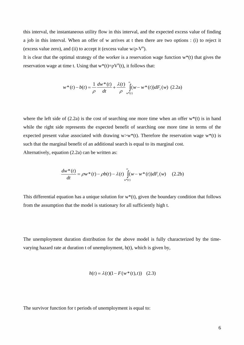
this interval, the instantaneous utility flow in this interval, and the expected excess value of finding

a job in this interval. When an offer of w arrives at t then there are two options : (i) to reject it

(excess value zero), and (ii) to accept it (excess value w/ρ-Vu).

It is clear that the optimal strategy of the worker is a reservation wage function w*(t) that gives the

reservation wage at time t. Using that w*(t)=ρVu(t), it follows that:

∫∞

−+=−)*(

)())(*()()(*1)()(*tw

t wdFtwwtdt

tdwtbtwρ

λρ

(2.2a)

where the left side of (2.2a) is the cost of searching one more time when an offer w*(t) is in hand

while the right side represents the expected benefit of searching one more time in terms of the

expected present value associated with drawing w>w*(t). Therefore the reservation wage w*(t) is

such that the marginal benefit of an additional search is equal to its marginal cost.

Alternatively, equation (2.2a) can be written as:

∫∞

−−−=)*(

)())(*()()()(*)(*

twt wdFtwwttbtw

dttdw λρρ (2.2b)

This differential equation has a unique solution for w*(t), given the boundary condition that follows

from the assumption that the model is stationary for all sufficiently high t.

The unemployment duration distribution for the above model is fully characterized by the time-

varying hazard rate at duration t of unemployment, h(t), which is given by,

))),(*(1)(()( ttwFtth −= λ (2.3)

The survivor function for t periods of unemployment is equal to:

6

))(exp()Pr(0∫−=>t

duuhTt (2.4)

and the density of the completed duration t is,

))(exp()())),(*(1)((exp()),(*(1)(()(00∫∫ −=−−−=tt

duuhthduuuwFuttwFttg λλ (2.5)

The likelihood function of a sample of durations for i unemployed workers, (ti, i=1,……,I), with no

incomplete spells of unemployment, is given by:

))(exp()(),.......,|)),(*(,),(),((01

1 ∫∏ −=−

itI

iiI duuhthttttwFttbL ρλ (2.6)

Clearly, using only duration data, the only identified parameter is the hazard rate, h(t), and none of

the structural parameters of the search model is identified (Flinn and Heckman, 1982).

In this setting the aggregate hazard rate may be duration dependent not only because of

heterogeneity of the hazard rate among individuals but also because the environment (parameters)

at individual level is not stationary. For example, the amount of unemployment benefits (bt)

depends on the elapsed duration and they are of limited duration: in this case it can be shown that

the reservation wage w*(t) declines (and the hazard therefore rises) up to the date of exhaustion.

Time variance of the arrival rate λt and the offer distribution F(.) over the entire duration of a spell

might also be realistic. It might be argued that employers interpret a long spell of unemployment

as a signal that a worker is a “lemon”, for example, in which case the arrival rate might be expected

to decline as a spell continues. Human capital might also diminished by the time out of work. Again,

a decline in the arrival rate of offers might be expected and the offer distribution might shift down

or change shape, as well. Alternatively, a worker (feeling either discouraged or desperate) may

adjust his or her search effort and methods over the course of a given spell. A worker may look

initially only into the best jobs available for a person with his or her skills, but look into less

desirable opportunities later in a spell. In either of these cases, the distribution of offers would

effectively vary with duration and the arrival rate might rise or decline or do both as a result of such

strategy changes. All of these considerations suggest that incorporating nonstationarity into the

model is appropriate.

7

Now consider again equation (2.3). It would obviously be useful for any empirical analysis of

unemployment durations to be able to separate between the two factors at the right-hand side, i.e. to

assess their relative magnitude for different types of individuals, as well as to assess the size of

policy effects on them. However, descriptive analysis of unemployment durations developed in this

paper simply restrict attention to variation of h itself over time and across individuals with different

observed characteristics x. The hazard function in particular is specified as a multiplicative

function of t, x. This defines the Proportional Hazard model, which is an ad hoc descriptive

statistics for h. In obvious notation:

)exp()(),( βxthxth t ′= (2.7)

This empirical approach raises an important issue. According to (2.3) the hazard rate h at t depends

on all structural parameters in a heavily non-linear fashion by way of the current reservation wage

w*(t). Even if these structural parameters are simple functions of t and/or x, this leads to a non-

proportional expression for h. Because the Proportional Hazard model parameters are not structural

parameters, a causal interpretation of the reduced-form estimates is problematic. The hazard is

proportional in t and x in the special case where ρ→∞. In that case workers do not care about the

future and even though they have information on future changes, this does not affect his optimal

strategy. The exit rate out of unemployment is:

)|),((),(),( xxtbFxtxth tλ= (2.8)

if λ(t,x) varies with t (e.g. because the long term unemployed are stigmatized) but not with x, and F

and b vary with x but not with t, the hazard is proportional in t and x. Alternatively, if F and b do

not depend on either t or x and λ is proportional in t and x, then the hazard is proportional as well.

Concluding the proportionality restriction of PH model cannot in general be justified on economic-

theoretical grounds. However, if the optimal strategy is myopic (e.g. because the discount rate is

infinite), then this restriction follows from non-stationary job search model described above.

8

3. Data

In 2001, ISTAT (see ISTAT, 2001), conducted the fourth survey on the transition of Italian

graduates into the labour market. The objective of the survey is to analyse the occupational position

of graduates three years after the completion of their university studies. Accordingly, the 2001

survey is conducted on those graduating in 1998. The graduate population of 1998 consisted of

105,097 individuals (49,393 males and 55,704 females). The ISTAT survey was based on a 25%

sample of these students and was stratified on the basis of university attended, degree course taken

and by sex of the individual student. The response rate was about 67%, yielding a data-set

containing information on 20,844 graduates. As a consequence the sample used in the present

analysis is not properly representative of the total population (although the ISTAT used a weighting

system for post-stratification to reduce the bias due to the non-response); so, the results presented in

the following sections should be considered with caution. The data contain information on: the

curriculum studied up to graduation in 1998, the occupational status and related work details by

2001, the search processes used between 1998 and 2001, the student’s family background and

personal characteristics.

For the present analysis, the sample of 20,000 records is reduced to 12,233 records by eliminating

the individuals who: (i) started their current jobs while at university, since their post-graduation

choices might be not comparable with those of the rest of the sample; (ii) declared that they were

not interested in finding a job; (iv) did report the information necessary for computing

unemployment duration and (v) didn’t go on to further education (master, phd, second degree,

school of specialization).

In the present paper, the object of interest is the time to obtain the first job. The latter is grouped in

quarters, because the survey indicates only the quarter of graduation and not its precise month. Here,

it is possible to distinguish between temporary and permanent jobs, but it is not provided

information on the contract type (part-time, full-time). The questionnaire allows us to make this

classification only with respect to the job held at the date of the interview, which is not necessarily

the first job. The graduates in 1998 were interviewed in December 2001, so the observable time to

obtain their first job ranges from 1 to 16 quarters. The time for the graduates who were still

unemployed at the date of interview is right censored and assumes a value between 12 and 16

depending on the quarter in which the individuals received their degree. The definitions of

covariates used in the analysis are reported in the appendix along with their sample means.

Concerning the covariates the following clarifications should be made : (1) there are not time-

varying covariates; (2) the dummy variable “military service” simply indicates whether the service

9

was done after the degree as opposed to either being done before the degree or that the student was

exempted from it; (3) the sample employed in the analysis has 15 groups of course programmes

which I have further grouped into 4 main categories9: Scientific, Engineering, Humanities, Social

sciences; (4) the geographical dummies refer to the University regions; (5) the dummy “mobility”

indicates whether the student transferred in another region to attend university; (6) parental

background is described by 7 categorical variable summarizing both parents’ educational level and

by father’s occupation; (7) as indicator of academic performance I used the variable “final mark”

(ranging from 66 to 110). The distribution of final mark is highly right skewed. This suggest that

there is a ceiling effect which weakens the correctness of this covariate as an indicator of academic

ability. To compensate partially for the previously mentioned deficiencies of the final mark, I used

also, as measures of ability, the score at high school and the type of high school (general,

vocational/technical or other)

4. Model specifications and methods of estimation

That the duration variable of interest (time to obtain the first job) is measured in quarters means that

the appropriate approach to modelling the duration of unemployment is the discrete-time hazard

model. The estimation of discrete-time duration models requires expanded or person-period data set

organized in such a way that there will be as many data rows for each individual in the sample as

there are time intervals over which the individual in question is at risk of experiencing the event of

interest (Jenkins 1997, 2003)- first job here. Following Meyer (1990), the discrete time hazard of

exiting the state of unemployment can be modelled using the discrete-time proportional hazards

model (PH specification, thereafter). In particular, the hazard of employment in the jth quarter, h(tj),

for individual i with a vector of covariates, x, having spent t quarters in unemployment and given

that employment has not occurred before tj-1 can be given by:

)))()(exp(exp(1 βγ ijij xth +−−= , where )(tjγ = (4.1) duuh )(0∫∞

∞−

)(tjγ represents the baseline hazard which can be specified either parametrically or semi-

parametrically.

9 The grouping in particular is the following: Scientic (chemistry, pharmacy, biology, agricultural, geology); Engineering (engineering, architecture); Social sciences (political sciences, sociology, law, economy and statistics); Humanities (literature, foreign languages, psychology, pedagogy).

10

I have assumed both parametric specification (log-polynomial) and a semi-parametric one

(piecewise constant) 10 . Rearranging (9) gives what is known as the complementary log-log

transformation of the conditional probability of exiting the state of unemployment at time tj as:

)())|(1ln(ln( txxth jiijij γβ +′=−− (4.2)

Given this complementary log-log transformation, the parameter β is interpreted as the effect of

covariates in x on the hazard rate of employment in interval j, assuming the hazard rate to be

constant over the jth interval. To check the correctness of the PH specification, I have also

estimated a discrete time logistic model, also known as proportional odds model. This specification

(originally developed only for the intrinsically discrete survival times and later applied also on

interval-censored data) assumes that the relative odds of making a transition in quarter j, given

survival up to end of the previous quarter, is:

)exp()0(1

)0(1 i

j

j

ij

ij xh

hh

hβ ′

⎥⎥⎦

⎤

⎢⎢⎣

⎡

−=

− (4.3)

where hij is the discrete time hazard rate for quarter j and hj(0) is the corresponding baseline hazard

arising when xi=0. The relative odds of making a transition at any given time is given by the

product of two components: (i) a relative odds that is common to all individuals, and (ii) an

individual-specific scaling factor. It follows that:

[ ] ijjij

ijij x

hh

hit βα ′+=⎥⎥⎦

⎤

⎢⎢⎣

⎡

−=

1loglog (4.4)

where αj=log[hj(0)/1-hj(0)]. We can write this expression, alternatively, as

)exp(11

ijij x

hβα ′−−+

= (4.5)

10 Several intervals have the same hazard, rather than differing in every interval. In this study the quarterly time period has been regrouped to get only 5 times periods. The rearranged time periods are: Quarter 1, Quarter 2-3, Quarter 4-7, Quarter 8-11, Quarter >12.

11

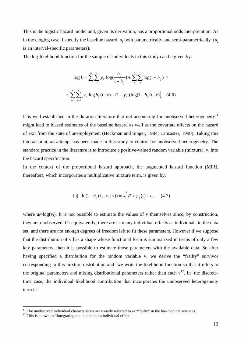
This is the logistic hazard model and, given its derivation, has a proportional odds interpretation. As

in the cloglog case, I specify the baseline hazard αj both parametrically and semi-parametrically (αj

is an interval-specific parameters).

The log-likelihood function for the sample of individuals in this study can be given by:

)1log()1

log(log ∑∑∑∑ −+−

=n

i

t

jij

n

i

t

j ij

ijit h

hh

yL =

= (4.6) [ ]∑∑= =

−−+n

i

t

jijijijit xthyxthy

1 1)|(1log()1()|(log

It is well established in the duration literature that not accounting for unobserved heterogeneity11

might lead to biased estimates of the baseline hazard as well as the covariate effects on the hazard

of exit from the state of unemployment (Heckman and Singer, 1984; Lancaster, 1990). Taking this

into account, an attempt has been made in this study to control for unobserved heterogeneity. The

standard practice in the literature is to introduce a positive-valued random variable (mixture), v, into

the hazard specification.

In the context of the proportional hazard approach, the augmented hazard function (MPH,

thereafter), which incorporates a multiplicative mixture term, is given by:

ijiijij utxvxth ++′=−− )())|,(1ln(ln( γβ (4.7)

where ui=log(vi). It is not possible to estimate the values of v themselves since, by construction,

they are unobserved. Or equivalently, there are as many individual effects as individuals in the data

set, and there are not enough degrees of freedom left to fit these parameters. However if we suppose

that the distribution of v has a shape whose functional form is summarized in terms of only a few

key parameters, then it is possible to estimate those parameters with the available data. So after

having specified a distribution for the random variable v, we derive the “frailty” survivor

corresponding to this mixture distribution and we write the likelihood function so that it refers to

the original parameters and mixing distributional parameters rather than each v12. In the discrete-

time case, the individual likelihood contribution that incorporates the unobserved heterogeneity

term is:

11 The unobserved individual characteristics are usually referred to as “frailty” in the bio-medical sciences. 12 This is known as “integrating out” the random individual effect.

12

duuguxthuxthL iuy

iijy

i

t

jiji

ijij )()))|,(1()|,((),,( 1−+∞

∞−

−=∆ ∫ ∏γβ (4.8)

where ∆ is the vector of unknown parameters in . The unobserved heterogeneity term is

assumed to be independent of observed covariates, , and the random duration variable, T, and

have density . In the absence of theoretical justification for using one or the other approach, I

assume two alternative parametric distribution: Gamma and Normal. If v has a Gamma distribution

with unit mean and variance σ

)( iu ug

ix

)( iu ug

2, as proposed by Meyer (1990), there is a closed form expression for

the frailty survivor function13:

[ ] 21

22 ),(ln1),|,( σσσβ−

−= XtSXtS (4.9).

With an inflow sample with right censoring, the contribution to the sample likelihood for a censored

observation i with spell length j intervals is S(tj, xi| β, σ2) and contribution of someone who makes

a transition in the jth interval is S(tj-1, xi | β, σ2)- S(tj, xi| β, σ2), with the appropriate substitution

made. Alternatively, I suppose that u has a Normal distribution with mean zero. In this case, there is

no convenient closed form expression for the survivor function and hence likelihood contributions:

the “integrating out” must be done numerically.

Finally I have also distinguished between two exit modes out of unemployment (fixed-term

contracts and open-ended contracts) estimating an independent competing risks model (ICR,

thereafter). Hence I have defined the cause-specific hazard function to destination fc (fixed

contracts) and to destination oc open-ended contracts as:

⎥⎥⎦

⎤

⎢⎢⎣

⎡−−= ∫

−

j

j

t

tfc

fcij dtth

1

)(exp1 θ (4.13)

⎥⎥⎦

⎤

⎢⎢⎣

⎡−−= ∫

−

j

j

t

toc

ocij dtth

1

)(exp1 θ (4.14)

where θfc and θoc are the underlying destination-specific continuous time hazard. The overall

discrete hazard and the survivor function for exit to any destination for tj are instead given by:

13

[ ] [ ]{ }ocij

fcijij hhh −−−= 1*11 (4.15)

ocij

fcijij SSS *= (4.16)

There are three types of contribution to the likelihood: that for an individual exiting to fixed-

contracts (Lfc), that for an individual exiting to open-ended contracts (Loc), and that for a censored

(Lc):

.17)

Toc, Tft and fft, foc are the destination-specific latent failure times and density functions

spectively. The lower integration point in the second integral, u, is the (unobserved) time within

== ijc SL oc

ijfc

ij SS *

dudvvfufdvvfufTTtTtL

dudvvfufdvvfufTTtTtL

j

j

j

j

j

j

j

j

t

t

t

u tocftocftocfcjocj

oc

t

t

t

u tocftocftftocjfcj

ft

∫ ∫ ∫

∫ ∫ ∫

−

∞

−

−

∞

−

⎥⎥⎦

⎤

⎢⎢⎣

⎡+=>≤<=

⎥⎥⎦

⎤

⎢⎢⎣

⎡+=>≤<=

11

11

)()()()(),Pr(

)()()()(),Pr(

(4

where

re

the interval at which the exit to fc/oc occurred. To proceed further, I make the assumption that

transitions can only occur at the boundaries of the intervals 14 . Then the overall likelihood

contribution for the person with a spell length tj is given by:

( ) ( ) ( )ocijoc

ij

ocijfc

ijfcij

fcij

ijocij

fcijij

Sh

hS

hh

LLLLocfc

ocfcocfc

δδ

δδδδ

⎥⎥⎦

⎤

⎢⎢⎣

⎡

−⎥⎥⎦

⎤

⎢⎢⎣

⎡

−=

=−−

11

1

(4.18)

artitions into a product of terms, each of which is a function of a single destination-specific hazard

where δfc and δoc are the destination-specific censoring indicators. Thus the likelihood contribution

p

only. Consequently, it is possible to estimate the overall independent competing risk model by

estimating separate destination-specific models having defined suitable destination-specific

censoring variables.

14 The assumption may not be an appropriate one in practice. So I have also estimated a multinomial logit model, originally developed for intrinsically discrete data. If the interval hazard rate was relatively small, this model may provide estimates that are a close approximation to a model for grouped-data with the assumption that the (continuous) hazard is constant within intervals.

14

As in the previous models, also in the competing risks one I have accommodated the presence of

observed individual heterogeneity assuming a multiplicative error term associated with each

. Estimation results and discussion

om estimation will be made. The first set of results in this

tudy is that which is based on non-parametric duration analysis, the second set is from single risk

.1 Non-parametric duration analysis

ration analysis I provide the estimates of the Life-table’s

urvivor and hazard functions in Table 1. They are the generalization of the Kaplan-Meier survivor

e quarters. If we look at the results for

results for course-program grouping. We

specific hazard function (Mixed Independent Competing Risk Model, MICR) . I further assume that

the errors are gamma distributed with mean 1 and variance σ2.

5

In this section discussion of results fr

s

duration models with and without unobserved heterogeneity (PH and MPH). Finally the third set of

results is from independent competing risk models with unobserved heterogeneity (MICR).

5

In the non-parametric approach to the du

s

and hazard functions for interval-censored data. Figure 1 and 2 give the plots of the aggregate and

disaggregated (by subject groups) Life-table’s survivor functions. The survivor function shows the

proportion of people who survive unemployment as time proceeds. The graph imply that graduates

in Humanities have the longest unemployment durations, followed by graduates in Social Sciences.

The survivor functions for graduates in Engineering and in Scientific subjects decline more steeply

than graduates from other groups implying that graduates in Engineering/Scientific subjects find

jobs sooner than graduates in other subjects. The figure also implies that for graduates in

Humanities, Social sciences, Scientific subjects and Engineering the probabilities of surviving

beyond 10 quarters are respectively: 0.40, 0.33, 0.28, 0,21.

Figure 3 and 4 provide the plots of the aggregate and disaggregated hazard functions. As we can see

from the graph for all data, the hazard rate increases over th

different subject groups, we observe that the hazard for graduates in engineering is larger than that

for graduates in other groups until about the 15th quarter.

The log-rank and the Wilcoxon tests allow for testing for the equality of two or more survivor

functions. Table 1 gives the log-rank and Wilcoxon tests

15

observe from the table that the null hypothesis of equality of survivor functions for different groups

is rejected by both tests.

5.2 Results from Proportional Hazard models

esults from the complementary log-log model,

ecause the proportional odds model provides almost equal estimates15.

I will discuss and report only the estimation r

b

The PH is estimated with two types of specification for the baseline hazard: the log-polynomial and

the piecewise constant exponential. The log-polynomial specification imposes a particular shape for

baseline hazard while the piecewise constant exponential provides a more flexible specification and

have an additional advantage in that parameters estimates are less sensitive to the distributional

assumptions made for unobserved heterogeneity. Both homogeneous and mixing proportional

hazards have been estimated. The mixing models estimated assumes that the distribution of the

unobserved heterogeneity is either normal or gamma or discrete. In the log-polynomial

specification without unobserved heterogeneity the estimated coefficients of ln(t), t^2 and t^3 reveal

that the baseline hazard decreases to a single minimum and then increases towards infinite

thereafter: a period of negative duration dependence is followed by positive duration dependence.

The same coefficients in the specifications with gamma unobserved heterogeneity are smaller in

absolute value terms, indicating a more marked positive dependence. Likelihood ratio test of zero

gamma unobserved heterogeneity is also rejected decisively underlying the importance of

accounting for unobserved heterogeneity. In the discrete distribution the coefficient of ln(t) is

positive, indicating only positive duration dependence.. If we suppose that the frailty term is

normally distributed the coefficients of duration dependence and of the covariates equal those of

the no-frailty model but in this case the likelihood ratio test suggests statistically not significant

frailty: the assumption that the unobserved heterogeneity is normally distributed is probably

incorrect . In the piecewise constant exponential specification, baseline hazard estimates under the

assumption of gamma and discrete mixing distribution are higher than those obtained under the

assumption of homogeneous and normal mixing distributions. The patterns of the baseline hazard

functions are shown in figure 6 where we can see that although there are some differences in the

magnitude of the estimated hazards from the different models, all the different baseline hazards

increase with time, after a short period of negative duration dependence. But accounting for

unobserved heterogeneity does increase the observed positive duration dependence. As such,

15 The 2 models provide similar estimates if the hazard is small. If h→0, the proportional odds model (logit(h)=log(h/1-h)=log(h)-log(1-h)), becomes a proportional hazard model.

16

therefore, these results are in line with the common claim in the literature that accounting for

unobserved heterogeneity increases positive duration dependence.

Results showing the estimated effects of covariates on the hazard of employment are given in Table

2, the

gree have a 37% (69%, 15%) lower hazard of employment

tistically

2 for the log-polynomial specification (with and without unobserved heterogeneity) and in Table 3

for the piecewise constant exponential none (with and without unobserved heterogeneity).

As can be seen from the estimation results of the log-polynomial specification in Table

estimated coefficients under the assumption of gamma mixing distribution are slightly larger in

absolute value terms with respect to those under the assumption of homogeneous and discrete

mixing distribution. Starting with the effect of personal characteristics on the hazard of exit out of

unemployment, older graduates are found to have a lower hazard of employment compared with

their younger counterparts: a one year rise in age is associated with a 7% (9%, 8%) lower hazard

rate in the homogeneous (gamma, discrete) model. So younger graduates find their first job earlier.

This could be explained by the fact that younger students are more likely to be better students

because they might have received their degree in the institutional time established for the course

programme they attended. These findings are in line with mine expectations. With regard to gender

differences, female graduates have a 13% (26%, 9%) lower hazard of employment compared with

male graduates in the homogeneous (gamma, discrete) model. An explanation for this that best fits

the labour economics literature is, of course, that men are generally expected to receive more job

offers than women do, mainly due to the female labour market behaviour that is (or perceived to be)

characterized by frequent interruptions.

Males who did their service after their de

with respect to males who did it before their degree or were exempted from military service in the

homogeneous (gamma, discrete) model. Actually, the starting date of military service is unknown,

but this lack of information is not a serious problem here since military service was 1 year long,

with the possible call occurring within 1 year after graduation; hence a military service covariate

equal to 1 indicates that the service started and ended within the observation period of the survey,

thus controlling for a definitely prior event. Graduates who transferred in another region to attend

university have a 6% (10%) higher hazard of finding their first job in the homogeneous (discrete)

model16. This could be explained by the fact that individuals who moved in another region to study

may be more motivated and better students than those who didn’t experience any transfer.

Considering the covariate related to academic ability, the final mark has not a sta

significant effect on the probability of obtaining the first job. The low influence of the final mark

16 This is not true if we consider the gamma model, where the variable mobility is not statistically significant.

17

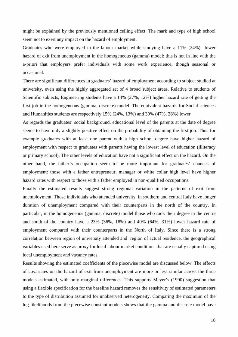
might be explained by the previously mentioned ceiling effect. The mark and type of high school

seem not to exert any impact on the hazard of employment.

Graduates who were employed in the labour market while studying have a 11% (24%) lower

hazard of exit from unemployment in the homogeneous (gamma) model: this is not in line with the

a-priori that employers prefer individuals with some work experience, though seasonal or

occasional.

There are significant differences in graduates’ hazard of employment according to subject studied at

university, even using the highly aggregated set of 4 broad subject areas. Relative to students of

Scientific subjects, Engineering students have a 14% (27%, 12%) higher hazard rate of getting the

first job in the homogeneous (gamma, discrete) model. The equivalent hazards for Social sciences

and Humanities students are respectively 15% (24%, 13%) and 30% (47%, 28%) lower.

As regards the graduates’ social background, educational level of the parents at the date of degree

seems to have only a slightly positive effect on the probability of obtaining the first job. Thus for

example graduates with at least one parent with a high school degree have higher hazard of

employment with respect to graduates with parents having the lowest level of education (illiteracy

or primary school). The other levels of education have not a significant effect on the hazard. On the

other hand, the father’s occupation seem to be more important for graduates’ chances of

employment: those with a father entrepreneur, manager or white collar high level have higher

hazard rates with respect to those with a father employed in non-qualified occupations.

Finally the estimated results suggest strong regional variation in the patterns of exit from

unemployment. Those individuals who attended university in southern and central Italy have longer

duration of unemployment compared with their counterparts in the north of the country. In

particular, in the homogeneous (gamma, discrete) model those who took their degree in the centre

and south of the country have a 23% (36%, 18%) and 40% (64%, 31%) lower hazard rate of

employment compared with their counterparts in the North of Italy. Since there is a strong

correlation between region of university attended and region of actual residence, the geographical

variables used here serve as proxy for local labour market conditions that are usually captured using

local unemployment and vacancy rates.

Results showing the estimated coefficients of the piecewise model are discussed below. The effects

of covariates on the hazard of exit from unemployment are more or less similar across the three

models estimated, with only marginal differences. This supports Meyer’s (1990) suggestion that

using a flexible specification for the baseline hazard removes the sensitivity of estimated parameters

to the type of distribution assumed for unobserved heterogeneity. Comparing the maximum of the

log-likelihoods from the piecewise constant models shows that the gamma and discrete model have

18

an edge over the other two models. As a result, I will discuss the covariate effects on the hazard

relying on the gamma and discrete model.

Male graduates who did their service after their degree have a 40% (18%) lower hazard of

employment with respect to males who did it before their degree or were exempted from military

service in the gamma (discrete) model. Older graduates are found to have a lower hazard of

employment compared with their younger counterparts. Women who are unemployed after

graduation have a 15% (7%) lower hazard of employment compared with their men counterparts.

Graduates who transferred in another region to attend university have a 6% (10%) higher hazard of

finding their first job in the homogeneous (discrete) model. As before, final mark at university and

high school have not a statistically significant effect on the hazard. Graduates who were employed

in the labour market while studying have a 9%(2%) lower hazard of exit from unemployment in

the gamma (discrete) model. Engineering graduates perform better in terms of unemployment

duration than graduates in Scientific subjects: the hazard of exit from unemployment of the former

is in fact 14% (8%) higher. The Social sciences and Humanities students have instead longer

duration of unemployment. As in the previous model, social background seems to exert an effect

on the hazard of employment only through father’s occupation: graduates with a father

entrepreneur, manager or white collar high level have more or less a 15% higher hazard of

employment compared with those with a father employed in non-qualified occupations. In terms of

regions, those who attended university in the central and Southern Italy tend to have longer

unemployment duration compared with their counterparts in the North of the country: Southern

Italian graduates, for example, have a 42% (30%) lower hazard of finding the first job in the gamma

(discrete).

5.3 Results Independent Competing Risks Models

I now consider the issue of destination state. Sample means of jobless duration and of number of

exits are given in Table 4. Comparing individuals entering in to fixed-term contracts with

individuals entering in to open-ended employment, it can be seen that their elapsed unemployment

duration is much longer. However, the most common form of transition is to open-ended contracts

rather than fixed-term employment.

The disaggregated version of the piecewise constant hazard regressions (under the assumption that

exits can occur at interval boundaries) are given in Table 4. The estimates correct for unobserved

19

heterogeneity 17 , assuming a gamma mixing distribution. It is immediately apparent that the

regression coefficients vary widely from destination state to destination state. Thus, for example,

the probability of finding employment in open-ended contracts is increasing with the level of

education of parents. But these effects of parental education are confined to open-ended contracts.

This is also true if we consider father’s occupation: having a father either entrepreneur or manager

or professional worker or white collar high level increases the hazard rate of open-ended

employment but not of fixed term contract. Female graduates have a higher hazard of exit to fixed

term contracts but a lower hazard of exit to open-ended employment compared to their male

counterparts. These findings caution against uncritical aggregation by destination state. Another

interesting result is that graduation in Engineering is associated with a sharply reduced likelihood of

entering into fixed-term contracts. The same is true for graduates in Social sciences. The probability

of escaping in to permanent jobs is negatively associated with graduation in Humanities. Mobility

increases only the probability of fixed term employment. Those who took their degree in the Centre

of Italy are less likely to enter open-ended employment than their Northern Italian counterparts, this

is not true if we consider exit to fixed-term contract. Southern graduates are less likely to exit to

both states, though this effect is more pronounced if we consider exit to open-unemployment

contract. Males who did their service after their degree are more penalized in terms of probability of

entering open-ended contracts: their hazard of exit into this state is 46% lower compared to males

who did it before their degree or were exempted from military service. The hazard of exit to fixed

term contracts instead is only 8% lower. As in the previous models, age and work experience while

at university have a negative effect on the hazard of exit from unemployment. The final mark at

university and high school are not statistically significant. Very similar results are obtained

estimating a multinomial logit model, under the assumptions that the interval-hazard is small and

that the continuous hazard is constant within intervals.

Baseline hazard functions, corresponding to the piecewise constant exponential specification, are

given in Figure 7. These results are obtained by setting all covariate values equal to zero. It is

apparent that the baseline hazards are both characterized by declining escape rates over the first

quarter, later there is evidence of positive duration dependence. Indeed, open-ended employment is

generally characterized by higher hazard rates with respect to those of fixed-contracts state.

However in the final quarters there is a sharp increase of hazard of exit to fixed-term contracts.

Taken in conjunction the two baseline hazards perhaps suggest that some graduates initially looking

for open-ended employment switch to sampling fixed-term contracts after a period of unsuccessful

search. 17 It is important to stress that in these models unobserved heterogeneity is not so important as in the previous one: the likelihood ratio test of zero unobserved heterogeneity for the gamma distribution is weakly rejected.

20

6. Conclusion

This paper attempted to analyse the duration of unemployment for Italian graduates. The focus of

the study has been on the time to obtain the first job, taking into account the graduates’

characteristics and the effects relating to course programmes. Parametric and non-parametric

discrete-time models have been used to study the hazard of exit to first job. Alternative mixing

distributions have also been employed to account for unobserved heterogeneity. The results

obtained indicate that there is evidence of positive duration dependence after a short initial period of

negative duration dependence. Accounting for unobserved heterogeneity does matter, but the main

finding to duration dependence remains unchanged. With regards to the effects of covariates, older

and female graduates, those who graduated in Humanities and Social sciences, those who had

fathers employed in non-qualified occupations , those males who did their service after their degree

and finally those who attended university in southern and central Italy are found to have particularly

lower hazard of getting their first job.

In addition, competing risk model with unobserved heterogeneity and semi-parametric baseline

hazard have been estimated to characterize transitions out of unemployment, accommodating

behaviourally distinct choices on the part of job seekers. Mine results reveal that the use of an

aggregate approach sometimes compound distinct and contradictory effects. Thus, for example, the

probability of finding employment in open-ended contracts is increasing with the level of education

of parents. But these effects are completely absent if we consider exit to fixed-term contracts.

Female graduates have a higher hazard of exit to fixed contracts but a lower hazard of exit to open-

ended employment compared to their male counterparts. Those who took their degree in the Centre

of Italy are less likely to enter open-ended employment than their Northern Italian counterparts, this

is not true if we consider exit to fixed term contract. Very similar results are obtained estimating a

multinomial logit model.

21

References

Allison, P. D. (1982), “Discrete-time methods for the analysis of event histories” Sociological

Methodology, 13, 61-98.

Biggeri L., Bini M. and Grilli L. (2000), “The transition from university to work: a multilevel

approach to the analysis of the time to obtain the first job”, J. R. Statistical Society A, 164, 293-305.

Boero G., McKnight A., Naylor R. and Smith J. (2001), “Graduates and Graduate Labour markets

in the UK and in Italy”, Crenos, Contributi di Ricerca 01/11.

Cox, D. R. (1972), “Regression models and life-tables” (with discussion), J. R. Statistical Society B,

34, 187-220.

Censis, “Rapporto sulla situazione del Paese, anno 1998”.

Devine, T.J. and N.M. Kiefer (1991), “Empirical Labor Economics”, Oxford University Press:

Oxford.

Dolton, P. J., Makepeace, G. H. and Treble, J. G. (1994) “The youth training scheme and the school

to work transition”, Oxford Economic Papers, 46,4, 629-657.

Eckstein, Z. and Van den Berg, (2003), “ Empirical Labor Search: A Survey”, IZA Discussion

Paper No. 929.

Firth, D. et al (1999), “Efficacy of programmes for the unemployed: discrete time modelling of

duration data from a matched comparison study. J. R. Statistic. Soc. A, 162, 111-120.

Han, A. and J. Hausman (1990), “Flexible Parametric Estimation of Duration and Competing Risk

Models”, Journal of Applied Econometrics, 5(1), 1-28.

Heckman, J. and B. Singer (1984a) “The identifiability of The Proportional Hazard Model”, Review

of Economic Studies, LI, 231-241.

22

Heckman, J. and B. Singer (1984b) “ A Method for Minimizing the Impact of Distributional

Assumptions in Econometric Models for Duration Data”, Econometrica, 52(2), 271-320.

ISTAT, “Rilevazione delle forze di lavoro, anno 1999”.

ISTAT, “Rapporto annuale, 1998”.

Jenkins, S. P. (1995), “Easy Estimation Methods for Discrete-Time Duration Models” Oxford

Bulletin of Economics and Statistics, 57(1), 129-138.

Jenkins, S. P. (1997), “sbe17: Estimation Methods for Discrete-Time (Grouped Duration Data)

Proportional Hazard Models: PGMHAZ”, Stata Technical Bulletin, 39, 1-12.

Jenkins, S. P. (2004) “Survival Analysis”, mimeo, Department of Economics, University of Essex,

UK.

Kiefer N. (1988) “Economic Duration Date and Hazard Functions”, Journal of economic Literature,

XXVI, 646-679.

Lancaster T. (1979), “Econometric Methods of the Duration of Unemployment” Econometrica,

47(4), 939-956.

Lancaster, T. (1990), “The Econometric Analysis of Transition Data”, Econometric Society

Monographs, Cambridge University Press, Cambridge.

Layder, D. et al. (1991), “ The empirical correlates of action and structure: the transition from

school to work”, Sociology, 25, 447-464.

Lynch, L. M. (1987), “Individual differences in the youth labour market: a cross-section analysis of

London youths”, From School to Unemployment?: the Labour Market for Young People, pp.185-

211. London: Macmillan.

Mealli, F. and Pudney S. (1999), “Specfication tests for random effects transition models: an

application to a model of the role of YTS in the youth labour market”. Lifetime Data Anal. 5, 213-

237.

23

Meyer, B. D. (1990), “Unemployment Insurance and Unemployment Spells” Econometrica 58:

757-782.

Narendranathan, W. and Stewart B. M. (1993a), “How Does the Unemployment Effect Vary as

Unemployment Spell Lenghtens?”, Journal of Applied Econometrics 8: 361-381.

Narendranathan, W. and Stewart B. M., 1993b “Modelling the Probability of Leaving

Unemployment: Competing Risks Models with Flexible Base-line Hazards”, Applied Statistics 42:

63-83.

Neumann, G. (1990), “Search Models and Duration Data”, Handbook of Applied Ecnometrics,

Chapter 4.

OCSE, Regard sur l’education, 1997.

Portugal P. and Addison J. (2003), “Six Ways to Leave Unemployment”, IZA Discussion Paper No

954.

Rogerson, R. and R. Wright (2001), “Search-theoretical models of the labor market”, Working

Paper, University of Pennsylvania, Philadelphia.

Santoro, M. and Pisati, M. (1996), “Dopo la laurea” Bologna: Il Mulino.

Tronti, L. and Mariani, P. (1994), “La transizione Università-Lavoro in Italia: un’esplorazione delle

evidenze dell’indagine ISTAT sugli sbocchi professionali dei laureati”, Econ. Lav., 25, no. 3, 3-26.

Van den Berg, G. (1990), “Nonstationary in Job Search Theory”, Review of Economic Studies, 57,

255-277.

Van den Berg, G. (2001), “Duration Models: Specification, Identification and Multiple Durations”,

in Handbook of Econometrics, edited by Heckman, James J. and Leamer Edward, V, North-Holland,

Amsterdam.

24

Wolpin, K. (1987), “Estimating a Structural Search Model: The Transition from School to Work”,

Econometrica, 55, 801-817.

25

Figure 1: Empirical Survivor Function.

0

0.2

0.4

0.6

0.8

1

1.2

1 2 3 4 5 6 7 8 9 10 11 12 13 14 15 16

Time to failure (in quarters)

Prob

abilit

Figure 2: Empirical Survivor Function by University Group.

0

0.2

0.4

0.6

0.8

1

1.2

1 2 3 4 5 6 7 8 9 10 11 12 13 14 15 16

Time to failure

Prob

abili

tie

Scientif ic Engineering Social sciences Humanities

26

Figure 3: Empirical Hazard Function.

0

0.5

1

1.5

2

2.5

1 2 3 4 5 6 7 8 9 10 11 12 13 14 15 16

Analysis Time (in quarters)

Haz

ard

Figure 4: Empirical Hazard Functions by University group.

0

0.5

1

1.5

2

2.5

1 2 3 4 5 6 7 8 9 10 11 12 13 14 15 16

Analysis time

Haz

ard

Scientif ic Engineering Social sciences Humanities

27

Figure 5: Baseline Hazard Functions in the log-polynomial specification under different

distributions for unobserved heterogeneity. .5

.6.7

.8.9

1ho

mog

en/n

orm

/gam

m/n

onpa

ra

0 5 10 15spell month identifier, by subject

homogen normgamm nonpara

Figure 6: Baseline Hazard Functions in the piecewise constant specification under different

distributions for unobserved heterogeneity.

.92

.94

.96

.98

1ga

mm

a/ho

mog

eneo

us/n

orm

al

0 5 10 15spell month identifier, by subject

gamma homogeneousnormal

28

Figure 7: Baseline Hazard Functions by Destination State.

.5.6

.7.8

.91

fixed

term

/ope

nend

ed

0 5 10 15spell month identifier, by subject

fixedterm openended

29

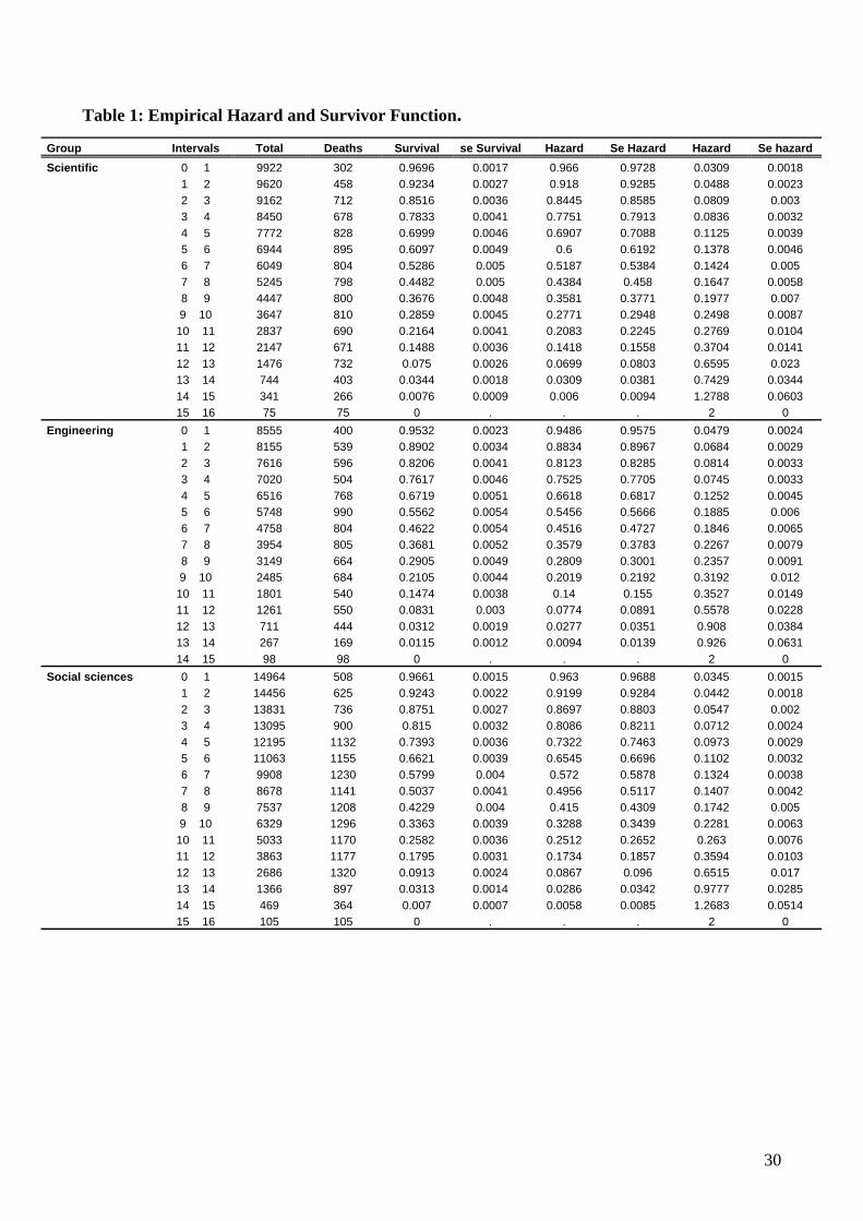
Table 1: Empirical Hazard and Survivor Function. Group Intervals Total Deaths Survival se Survival Hazard Se Hazard Hazard Se hazard Scientific 0 1 9922 302 0.9696 0.0017 0.966 0.9728 0.0309 0.0018 1 2 9620 458 0.9234 0.0027 0.918 0.9285 0.0488 0.0023 2 3 9162 712 0.8516 0.0036 0.8445 0.8585 0.0809 0.003 3 4 8450 678 0.7833 0.0041 0.7751 0.7913 0.0836 0.0032 4 5 7772 828 0.6999 0.0046 0.6907 0.7088 0.1125 0.0039 5 6 6944 895 0.6097 0.0049 0.6 0.6192 0.1378 0.0046 6 7 6049 804 0.5286 0.005 0.5187 0.5384 0.1424 0.005 7 8 5245 798 0.4482 0.005 0.4384 0.458 0.1647 0.0058 8 9 4447 800 0.3676 0.0048 0.3581 0.3771 0.1977 0.007 9 10 3647 810 0.2859 0.0045 0.2771 0.2948 0.2498 0.0087 10 11 2837 690 0.2164 0.0041 0.2083 0.2245 0.2769 0.0104 11 12 2147 671 0.1488 0.0036 0.1418 0.1558 0.3704 0.0141 12 13 1476 732 0.075 0.0026 0.0699 0.0803 0.6595 0.023 13 14 744 403 0.0344 0.0018 0.0309 0.0381 0.7429 0.0344 14 15 341 266 0.0076 0.0009 0.006 0.0094 1.2788 0.0603 15 16 75 75 0 . . . 2 0 Engineering 0 1 8555 400 0.9532 0.0023 0.9486 0.9575 0.0479 0.0024 1 2 8155 539 0.8902 0.0034 0.8834 0.8967 0.0684 0.0029 2 3 7616 596 0.8206 0.0041 0.8123 0.8285 0.0814 0.0033 3 4 7020 504 0.7617 0.0046 0.7525 0.7705 0.0745 0.0033 4 5 6516 768 0.6719 0.0051 0.6618 0.6817 0.1252 0.0045 5 6 5748 990 0.5562 0.0054 0.5456 0.5666 0.1885 0.006 6 7 4758 804 0.4622 0.0054 0.4516 0.4727 0.1846 0.0065 7 8 3954 805 0.3681 0.0052 0.3579 0.3783 0.2267 0.0079 8 9 3149 664 0.2905 0.0049 0.2809 0.3001 0.2357 0.0091 9 10 2485 684 0.2105 0.0044 0.2019 0.2192 0.3192 0.012 10 11 1801 540 0.1474 0.0038 0.14 0.155 0.3527 0.0149 11 12 1261 550 0.0831 0.003 0.0774 0.0891 0.5578 0.0228 12 13 711 444 0.0312 0.0019 0.0277 0.0351 0.908 0.0384 13 14 267 169 0.0115 0.0012 0.0094 0.0139 0.926 0.0631 14 15 98 98 0 . . . 2 0 Social sciences 0 1 14964 508 0.9661 0.0015 0.963 0.9688 0.0345 0.0015 1 2 14456 625 0.9243 0.0022 0.9199 0.9284 0.0442 0.0018 2 3 13831 736 0.8751 0.0027 0.8697 0.8803 0.0547 0.002 3 4 13095 900 0.815 0.0032 0.8086 0.8211 0.0712 0.0024 4 5 12195 1132 0.7393 0.0036 0.7322 0.7463 0.0973 0.0029 5 6 11063 1155 0.6621 0.0039 0.6545 0.6696 0.1102 0.0032 6 7 9908 1230 0.5799 0.004 0.572 0.5878 0.1324 0.0038 7 8 8678 1141 0.5037 0.0041 0.4956 0.5117 0.1407 0.0042 8 9 7537 1208 0.4229 0.004 0.415 0.4309 0.1742 0.005 9 10 6329 1296 0.3363 0.0039 0.3288 0.3439 0.2281 0.0063 10 11 5033 1170 0.2582 0.0036 0.2512 0.2652 0.263 0.0076 11 12 3863 1177 0.1795 0.0031 0.1734 0.1857 0.3594 0.0103 12 13 2686 1320 0.0913 0.0024 0.0867 0.096 0.6515 0.017 13 14 1366 897 0.0313 0.0014 0.0286 0.0342 0.9777 0.0285 14 15 469 364 0.007 0.0007 0.0058 0.0085 1.2683 0.0514 15 16 105 105 0 . . . 2 0

30

Table 1: Empirical Hazard and Survivor Function (continuing).

Humanities 0 1 9709 286 0.9705 0.0017 0.967 0.9737 0.0299 0.0018 1 2 9423 295 0.9402 0.0024 0.9353 0.9447 0.0318 0.0019 2 3 9128 382 0.9008 0.003 0.8947 0.9066 0.0427 0.0022 3 4 8746 516 0.8477 0.0036 0.8404 0.8547 0.0608 0.0027 4 5 8230 576 0.7883 0.0041 0.7801 0.7963 0.0725 0.003 5 6 7654 705 0.7157 0.0046 0.7066 0.7246 0.0966 0.0036 6 7 6949 690 0.6447 0.0049 0.635 0.6541 0.1045 0.004 7 8 6259 749 0.5675 0.005 0.5576 0.5773 0.1273 0.0046 8 9 5510 760 0.4892 0.0051 0.4793 0.4991 0.1481 0.0054 9 10 4750 837 0.403 0.005 0.3933 0.4128 0.1932 0.0066 10 11 3913 750 0.3258 0.0048 0.3165 0.3351 0.212 0.0077 11 12 3163 1034 0.2193 0.0042 0.2111 0.2276 0.3908 0.0119 12 13 2129 864 0.1303 0.0034 0.1237 0.1371 0.5091 0.0168 13 14 1265 650 0.0633 0.0025 0.0586 0.0683 0.6915 0.0254 14 15 615 420 0.0201 0.0014 0.0174 0.023 1.037 0.0433 15 16 195 195 0 . . . 2 0

Table 1.2: Log-rank and Wilcoxon (Breslow) tests.

Log-rank test for equality of survivor functions Events Events observed expected

Scientific 2412 2297.88

Engineering 2364 1929.52 Social sciences 3414 3565.97

Humanities 1973 2369.62 Total 10163 10163

chi2(4) = 235.88

Pr>chi2 = 0

Wilcoxon (Breslow) test Events Events Sum of observed expected ranks

Scientific 2412 2297.88 487960

Engineering 2364 1929.52 3361126 Social sciences 3414 3565 -1138396

Humanities 1973 2369 -2710691 Total

chi2(4)= 197.97

Pr>chi2= 0

31

Table 2: Results of the log-polynomial specification.

Homogeneous Normal Mixing Gamma Mixing Discrete Mixing Variables

Coefficient P-value Coefficient P-value Coefficient P-value Coefficient P-value

duration dependence: lnt -0.3713239

0 -0.3713235 0 0.137376 0.178 1.463355 0t2 0.005547 0.118 0.005547 0.132 0.0131462 0.013 -0.0514121 0t3 0.0005625 0.017 0.0005625 0.023 0.0012968 0.001 0.0036226 0personal characteristics:

mobility 0.0605954 0.066 0.0605954 0.066 0.0345276 0.558 0.1001772 0.021militaryser -0.4558916 0 -0.4558922 0 -1.142401 0 -0.156995 0.019age -0.0739731 0 -0.0739732 0 -0.091646 0 -0.085537 0sex -0.1430251 0 -0.1430253 0 -0.3022407 0 -0.0915983 0.078workduruniversity -0.0760083 0.023 -0.0760084 0.023 -0.2297479 0 -0.0145281 0.742university final mark -0.0022069 0.365 -0.0022069 0.365 0.0028349 0.523 -0.0059673 0.058high school final mark 0.001732 0.486 0.001732 0.488 0.0048935 0.275 -0.0003074 0.924 high school type: general high school 0.0361103 0.528 0.0361104 0.524 0.0561997 0.574 0.0294945 0.69vocational/tech high school 0.0425121 0.49 0.0425122 0.485 0.1055892 0.326 -0.0025692 0.974 university group:

Engineering 0.1361557 0.007 0.1361558 0.006 0.2463231 0.007 0.1214982 0.065Social sciences -0.161083 0 -0.1610832 0 -0.2625992 0.001 -0.1299539 0.046Humanities -0.3469408 0 -0.3469412 0 -0.6209759 0 -0.3199328 0university (grouped by region)

northeast -0.1305612 0.002 -0.1305614 0.002 -0.2551981 0.001 -0.0793899 0.17centre -0.2505108 0 -0.2505111 0 -0.4419531 0 -0.1892606 0.002south -0.497394 0 -0.4973946 0 -1.003321 0 -0.3644468 0parents' education: parentaleducation2 0.0385912 0.536 0.0385914 0.536 0.1343415 0.232 -0.006013 0.944parentaleducation3 0.1032177 0.074 0.1032178 0.074 0.19224 0.064 0.0780934 0.278parentaleducation4 -0.0028894 0.962 -0.0028893 0.962 0.0516643 0.624 -0.0591301 0.455parentaleducation5 0.0616191 0.342 0.0616192 0.338 0.1315848 0.248 0.0705464 0.397parentaleducation6 -0.0926146 0.222 -0.0926146 0.216 -0.0679371 0.607 -0.0754829 0.436parentaleducation7 0.0699367 0.44 0.0699369 0.435 0.349604 0.032 -0.0604858 0.615father's occupation:

entrepreneur 0.1391532 0.067 0.1391534 0.067 0.4615475 0.001 0.0471155 0.622professional worker 0.0643941 0.431 0.0643941 0.426 0.2396845 0.102 -0.0191005 0.851own-account worker

0.0143088 0.811 0.0143088 0.811 0.1141972 0.287 -0.0811998 0.346

manager 0.1401497 0.049 0.1401499 0.049 0.3404123 0.008 0.0192349 0.842

teacher/professor

-0.0112486 0.901 -0.0112485 0.9 0.0454078 0.77 -0.0296727 0.813white collar high level

0.1291801 0.046 0.1291802 0.045 0.2346982 0.041 0.1431497 0.081

white collar low level 0.1022502 0.138 0.1022503 0.136 0.2853773 0.021 0.0096954 0.918blue collar high level 0.0443426 0.458 0.0443427 0.458 0.1695161 0.117 0.0086675 0.913constant 1.449309 0.007 1.44931 0.007 2.018419 0.04variance 1.186 0.1216mass point 1 location 0.28236 mass point 1 probability 0.7183 mass point 2 location 4.0212 mass point 2 probability 0.2817 no of person-period obs 18382 18382 18382 18382

Log-likelihood -9363.65 -9363.65 -9327.98 -8950.61

33

Table 3: Results of the Piecewise Constant Exponential specification.

Homogeneous Normal Mixing Gamma Mixing Discrete Mixing Variables

Coefficient P-value Coefficient P-value Coefficient P-value Coefficient P-value

duration dependence: quarter 1 1.396332

0.009 1.396334 0.01 1.491261 0.01 . .quarter 2-3 0.9452248 0.079 0.9452264 0.081 1.060764 0.068 2.241067 0quarter 4-7 1.099418 0.041 1.09942 0.042 1.24701 0.034 2.463152 0quarter 8-11 1.399149 0.01 1.399152 0.01 1.593195 0.009 2.767759 0quarter >=12 2.466148 0 2.466152 0 2.721224 0 3.838766 0personal characteristics:

mobility 0.0563571 0.087 0.0563571 0.087 0.0571556 0.097 0.0995347 0.013militaryser

-0.4599618 0 -0.4599624 0 -0.4976171 0 -0.1877149 0.003

age -0.0715951 0 -0.0715951 0 -0.0742632 0 -0.0758514 0sex -0.1443971 0 -0.1443973 0 -0.1556474 0 -0.069465 0.15workduruniversity -0.0789204 0.018 -0.0789205 0.018 -0.0882735 0.015 -0.0136736 0.735university final mark -0.0019358 0.427 -0.0019358 0.427 -0.0017881 0.484 -0.0061158 0.034high school final mark 0.0020806 0.404 0.0020806 0.405 0.0023061 0.379 0.0007023 0.811high school type: general high school 0.0334584 0.558 0.0334585 0.555 0.0372443 0.529 0.0554095 0.393vocational/tech high school 0.0402268 0.513 0.0402269 0.508 0.0462647 0.468 0.0159961 0.821university group:

Engineering 0.1311232 0.009 0.1311232 0.008 0.1326834 0.011 0.0804768 0.194Social sciences -0.1601668 0 -0.160167 0 -0.1712497 0 -0.1570826 0.007Humanities -0.3391952 0 -0.3391955 0 -0.3584985 0 -0.2875712 0university (grouped by region)

northeast -0.1308441 0.002 -0.1308442 0.002 -0.1403498 0.002 -0.0813967 0.134centre -0.2519251 0 -0.2519253 0 -0.2673039 0 -0.2011342 0south -0.4970476 0 -0.4970481 0 -0.529359 0 -0.3429432 0parents' education: parentaleducation2 0.0440601 0.48 0.0440602 0.479 0.0494966 0.449 -0.0058518 0.937parentaleducation3 0.1019983 0.078 0.1019984 0.077 0.1077914 0.076 0.0561801 0.398parentaleducation4 0.0010658 0.986 0.0010658 0.986 0.0060523 0.923 -0.0568167 0.429parentaleducation5 0.0630304 0.332 0.0630304 0.327 0.0678331 0.314 0.0336632 0.662parentaleducation6 -0.0911415 0.23 -0.0911415 0.223 -0.0920959 0.238 -0.1092295 0.21parentaleducation7 0.0741298 0.413 0.0741301 0.407 0.0908353 0.34 -0.1067609 0.34father's occupation:

entrepreneur 0.1381534 0.069 0.1381536 0.068 0.1531335 0.059 0.00336 0.97professional worker 0.0657697 0.421 0.0657697 0.416 0.0702658 0.406 -0.004108 0.965

34

own-account worker

0.0181939 0.761 0.018194 0.761 0.0230814 0.712 -0.0561046 0.452manager 0.137115 0.054 0.1371152 0.054 0.1479736 0.049 0.0311304 0.722teacher/professor -0.0058115 0.949 -0.0058115 0.948 -0.003706 0.968 -0.0069444 0.95white collar high level

0.1254186 0.053 0.1254187 0.051 0.1304732 0.053 0.1137459 0.129

white collar low level 0.1047343 0.128 0.1047345 0.127 0.1158522 0.111 0.0173228 0.835blue collar high level

0.0409122 0.494 0.0409122 0.493 0.0460699 0.462 -0.0313738 0.65

variance 0.1206mass point 1 location -1.0243 mass point 1 probability 0.7329 mass point 2 location 3.9309 mass point 2 probability 0.2671 no of person-period obs 18382 18382 18382 18382

Log-likelihood -9384.14 -9384.14 -9383.72 -8991.9

35

Table 4: Independent Competing Risks model results.

Fixed-term contract Open-ended contract Variables Coefficient P-value Coefficient P-value

duration dependence: quarter 1 0.0528139 0.957 0.7172376 0.349 quarter 2-3 -0.4518352 0.646 0.4091341 0.594 quarter 4-7 -0.2567898 0.794 0.6387147 0.409 quarter 8-11 0.1864805 0.85 0.9652161 0.22 quarter >=12 1.134588 0.255 2.019738 0.013 personal characteristics: mobility 0.1319883 0.017 0.007677 0.868 militaryser -0.0681394 0.476 -0.7387421 0 age -0.0826791 0.001 -0.0583311 0.004 sex 0.2075161 0.003 -0.3632243 0 workduruniversity -0.0961502 0.089 -0.0819158 0.084 university final mark -0.00245 0.575 -0.0003559 0.916 high school final mark 0.0029212 0.498 0.0017133 0.624 high school type: general high school 0.0657697 0.461 0.014983 0.854 vocational/tech high school 0.074985 0.445 0.029356 0.735 university group: Engineering -0.1734739 0.046 0.278211 0 Social sciences -0.3377125 0 -0.0696799 0.276 Humanities -0.122266 0.142 -0.5558422 0 university (grouped by region) northeast -0.0140339 0.845 -0.2089908 0 centre -0.0967604 0.23 -0.3702685 0 south -0.3096046 0 -0.6586075 0 parents' education: parentaleducation2 -0.0895483 0.375 0.1551497 0.083 parentaleducation3 -0.054915 0.56 0.2107057 0.011 parentaleducation4 -0.0609184 0.528 0.0548163 0.521 parentaleducation5 -0.1448043 0.179 0.1931947 0.034 parentaleducation6 -0.2064596 0.099 -0.000982 0.993 parentaleducation7 -0.127923 0.405 0.2481774 0.052 father's occupation: entrepreneur -0.0597728 0.649 0.3134268 0.004 professional worker -0.2552855 0.076 0.264883 0.018 own-account worker -0.0534574 0.575 0.0735499 0.392 manager 0.0189445 0.873 0.2340791 0.02 teacher/professor -0.0248452 0.867 0.0326851 0.795 white collar high level -0.0583722 0.589 0.2527128 0.006 white collar low level -0.0156941 0.89 0.2116538 0.032 blue collar high level 0.0110923 0.907 0.0775643 0.369 no of person-period obs 18382 18382

Log-likelihood -4973.994 -7311.64

first job status noexit exit Total mean duration unemployed 100 0 17.86 16 (0) fixed-term 0 35.6 29.24 4.6 (3.9)

open-ended 0 64.4 52.9 4 (3.5)

17.86

82.14 100

Appendix: Definitions of the covariates and sample averages.

Name and definition Average Time (in quarters, from 0 to 16) 7.204209Mobility (1, transfer in another region; 0 otherwise) 1.493919Sex (0, male; 1, female) 1.522089Military service (0, done before degree or exempted from; 1, done after degree) 0.1592793Age 28.41297University final mark (integers from 66 to 110) 102.615High school mark (integers from 36 to 60) 48.81282General high school 0.5913778Vocational/technical high school 0.2902523Other high school 0.1183699Workduruniversity (1, the graduate held at least one job during university studies, 0, otherwise) 0.434408 Parentaleduc1 (both parents illiterate or with primary school certificate) 0.1461798 Parentaleduc2 (at least one parent with middle school certificate) 0.0978303Parentaleduc3 (both parents with a middle school certificate) 0.148035Parentaleduc4 (at least one parent with a high school certificate) 0.1897102Parentaleduc5 (both parents with high school certificate) 0.175728Parentaleduc6 (at least one parent with a degree) 0.1605014Parentaleduc7 (both parents with a degree) 0.0820154North-west (university in the north-west of Italy) 0.2653061 North-east (university in the north-east of Italy) 0.2398695Centre (university in the centre of Italy) 0.2396883South (university in the south of Italy) 0.255136Scientific (graduation in scientific subjects) 0.2277312Engineering (graduation in engineering) 0.1953137Social sciences (graduation in social, economic and political subjects) 0.3496057Humanities (graduation in humanities) 0.2273493entrepreneur 0.0531305professional worker 0.079752own-account worker 0.1284793manager 0.1402062teacher/professor 0.0636443white collar high level 0.1586952white collar low level 0.0943994blue collar high level 0.1373981

other occupation 0.15166

37