
The Traditional Approach to Consumer Theory · Chapter 3 The Traditional Approach to Consumer...
58
Chapter 3 The Traditional Approach to Consumer Theory In the previous section, we considered consumer behavior from a choice-based point of view. That is, we assumed that consumers made choices about which consumption bundle to choose from a set of feasible alternatives, and, using some rather mild restrictions on choices (homogeneity of degree zero, Walras’ law, and WARP), were able make predictions about consumer behavior. Notice that our predictions were entirely based on consumer behavior. In particular, we never said anything about why consumers behave the way they do. We only hold that the way they behave should be consistent in certain ways. The traditional approach to consumer behavior is to assume that the consumer has well-defined preferences over all of the alternative bundles and that the consumer attempts to select the most preferred bundle from among those bundles that are available. The nice thing about this approach is that it allows us to build into our model of consumer behavior how the consumer feels about trading off one commodity against another. Because of this, we are able to make more precise predictions about behavior. However, at some point people started to wonder whether the predictions derived from the preference-based model were in keeping with the idea that consumers make consistent choices, or whether there could be consistent choice-based behavior that was not derived from the maximization of well-defined preferences. It turns out that if we define consistent choice making as homogeneity of degree zero, Walras’ law, and WARP, then there are consistent choices that cannot be derived from the preference-based model. But, if we replace WARP with a slightly stronger but still reasonable condition, called the Strong Axiom of Revealed Preference (SARP), 29
Transcript of The Traditional Approach to Consumer Theory · Chapter 3 The Traditional Approach to Consumer...

Chapter 3
The Traditional Approach to
Consumer Theory
In the previous section, we considered consumer behavior from a choice-based point of view. That
is, we assumed that consumers made choices about which consumption bundle to choose from a set
of feasible alternatives, and, using some rather mild restrictions on choices (homogeneity of degree
zero, Walras’ law, and WARP), were able make predictions about consumer behavior. Notice that
our predictions were entirely based on consumer behavior. In particular, we never said anything
about why consumers behave the way they do. We only hold that the way they behave should be
consistent in certain ways.
The traditional approach to consumer behavior is to assume that the consumer has well-defined
preferences over all of the alternative bundles and that the consumer attempts to select the most
preferred bundle from among those bundles that are available. The nice thing about this approach is
that it allows us to build into our model of consumer behavior how the consumer feels about trading
off one commodity against another. Because of this, we are able to make more precise predictions
about behavior. However, at some point people started to wonder whether the predictions derived
from the preference-based model were in keeping with the idea that consumers make consistent
choices, or whether there could be consistent choice-based behavior that was not derived from the
maximization of well-defined preferences. It turns out that if we define consistent choice making
as homogeneity of degree zero, Walras’ law, and WARP, then there are consistent choices that
cannot be derived from the preference-based model. But, if we replace WARP with a slightly
stronger but still reasonable condition, called the Strong Axiom of Revealed Preference (SARP),
29
Nolan Miller Notes on Microeconomic Theory: Chapter 3 ver: Aug. 2006
then any behavior consistent with these principles can be derived from the maximization of rational
preferences.
Next, we take up the traditional approach to consumer theory, often called “neoclassical” con-
sumer theory.
3.1 Basics of Preference Relations
We’ll continue to assume that the consumer chooses from among L commodities and that the
commodity space is given by X ⊂ RL+. The basic idea of the preference approach is that given any
two bundles, we can say whether the first is “at least as good as” the second. The “at-least-as-
good-as” relation is denoted by the curvy greater-than-or-equal-to sign: º. So, if we write x º y,
that means that “x is at least as good as y.”
Using º, we can also derive some other preference relations. For example, if x º y, we
could also write y ¹ x, where ¹ is the “no better than” relation. If x º y and y º x, we say
that a consumer is “indifferent between x and y,” or symbolically, that x ∼ y. The indifference
relation is important in economics, since frequently we will be concerned with indifference sets.
The indifference curve Iy is defined as the set of all bundles that are indifferent to y. That is,
Iy = {x ∈ X|y ∼ x}. Indifference sets will be very important as we move forward, and we will
spend a great deal of time and effort trying to figure out what they look like, since the indifference
sets capture the trade-offs the consumer is willing to make among the various commodities. The
final preference relation we will use is the “strictly better than” relation. If x is at least as good
as y and y is not at least as good as x, i.e., x º y and not y º x (which we could write y ² x), we
say that x  y, or x is strictly better than (or strictly preferred to) y.
Our preference relations are all examples of mathematical objects called binary relations. A
binary relation compares two objects, in this case, two bundles. For instance, another binary
relation is “less-than-or-equal-to,” ≤. There are all sorts of properties that binary relations can
have. The first two we will be interested in are called completeness and transitivity. A binary
relation is complete if, for any two elements x and y in X, either x º y or y º x. That is, any two
elements can be compared. A binary relation is transitive if x º y and y º z imply x º z. That
is, if x is at least as good as y, and y is at least as good as z, then x must be at least as good as z.
The requirements of completeness and transitivity seem like basic properties that we would like
any person’s preferences to obey. This is true. In fact, they are so basic that they form economists’
30

Nolan Miller Notes on Microeconomic Theory: Chapter 3 ver: Aug. 2006
very definition of what it means to be rational. That is, a preference relation º is called rational
if it is complete and transitive.
When we talked about the choice-based approach, we said that there was implicit in the idea
that demand functions satisfy Walras Law the idea that “more is better.” This idea is formalized
in terms of preferences by making assumptions about preferences over one bundle or another.
Consider the following property, called monotonicity:
Definition 5 A preference relation º is monotone if x  y for any x and y such that xl > yl
for l = 1, ..., L. It is strongly monotone if xl ≥ yl for all l = 1, ..., L and xj > yj for some
j ∈ {1, ..., L} implies that x  y.
Monotonicity and strong monotonicity capture two different notions of “more is better.” Monotonic-
ity says that if every component of x is larger than the corresponding component of y, then x is
strictly preferred to y. Strong monotonicity is the requirement that if every component of x is at
least as large (but not necessarily strictly larger) than the corresponding component of y and at
least one component of x is strictly larger, x is strictly preferred to y.
The difference between monotonicity and strong monotonicity is illustrated by the following
example. Consider the bundles x = (1, 1) and y = (1, 2). If º is strongly monotone, then we
can say that y  x. However, if º is monotone but not strongly monotone, then it need not be
the case that y is strictly preferred to x. Since preference relations that are strongly monotone
are monotone, but preferences that are monotone are not necessarily strongly monotone, strong
monotonicity is a more restrictive (a.k.a. “stronger”) assumption on preferences.
If preferences are monotone or strongly monotone, it follows immediately that a consumer will
choose a bundle on the boundary of the Walrasian budget set. Hence an assumption of some sort
of monotonicity must have been in the background when we assumed consumer choices obeyed
Walras’ Law. However, choice behavior would satisfy Walras’ Law even if preferences satisfied the
following weaker condition, called local nonsatiation.
Condition 6 A preference relation º satisfies local nonsatiation if for every x and every ε > 0
there is a point y such that ||x− y|| ≤ ε and y  x.
That is, for every x, there is always a point “nearby” that the consumer strictly prefers to x,
and this is true no matter how small you make the definition of “nearby.” Local nonsatiation allows
for the fact that some commodities may be “bads” in the sense that the consumer would sometimes
31

Nolan Miller Notes on Microeconomic Theory: Chapter 3 ver: Aug. 2006
prefer less of them (like garbage or noise). However, it is not possible for all goods to always be
bads if preferences are non-satiated. (Why?)
It’s time for a brief discussion about the practice of economic theory. Recall that the object
of doing economic theory is to derive testable implications about how real people will behave.
But, as we noted earlier, in order to derive testable implications, it is necessary to impose some
restrictions on (make assumptions about) the type of behavior we allow. For example, suppose we
are interested in the way people react to wealth changes. We could simply assume that people’s
behavior satisfies Walras’ Law, as we did earlier. This allows us to derive testable implications.
However, it provides little insight into why they satisfy Walras’ Law. Another option would be
to assume monotonicity — that people prefer more to less. Monotonicity implies that people will
satisfy Walras’ Law. But, it rules out certain types of behavior. In particular, it rules out the
situation where people prefer less of an object to more of it. But, introspection tells us that
sometimes we do prefer less of something. So, we ask ourselves if there is a weaker assumption
that allows people to prefer less to more, at least sometimes, that still implies Walras’ Law. It
turns out that local nonsatiation is just such an assumption. It allows for people to prefer less to
more — even to prefer less of everything — the only requirement is that, no matter which bundle the
consumer currently selects, there is always a feasible bundle nearby that she would rather have.
By selecting the weakest assumption that leads to a particular result, we accomplish two tasks.
First, the weaker the assumptions used to derive a result, the more “robust” it is, in the sense that
a greater variety of initial conditions all lead to the same conclusion. Second, finding the weakest
possible condition that leads to a particular conclusion isolates just what is needed to bring about
the conclusion. So, all that is really needed for consumers to satisfy Walras’ Law is for preferences
to be locally nonsatiated — but not necessarily monotonic or strongly monotonic.
The assumptions of monotonicity or local nonsatiation will have important implications for the
way indifference sets look. In particular, they ensure that Ix = {y ∈ X|y ∼ x} are downward
sloping and “thin.” That is, they must look like Figure 3.1.
If the indifference curves were thick, as in Figure 3.2, then there would be points such as x,
where in a neighborhood of x (the dotted circle) all points are indifferent to x. Since there is no
strictly preferred point in this region, it is a violation of local-nonsatiation (or monotonicity).
In addition to the indifference set Ix defined earlier, we can also define upper-level sets and
lower-level sets. The upper level set of x is the set of all points that are at least as good as
x, Ux = {y ∈ X|y º x} . Similarly, the lower level set of x is the set of all points that are no
32

Nolan Miller Notes on Microeconomic Theory: Chapter 3 ver: Aug. 2006
x2
x1
Ix
Figure 3.1: Thin Indifferent Sets
x2
x1
Ix
x
Figure 3.2: Thick Indifference Sets
33

Nolan Miller Notes on Microeconomic Theory: Chapter 3 ver: Aug. 2006
better than x, Lx = {y ∈ X|x º y}. Just as monotonicity told us something about the shape of
indifference sets, we can also make assumptions that tell us about the shape of upper and lower
level sets.
Recall that a set of points, X, is convex if for any two points in the set the (straight) line
segment between them is also in the set.1 Formally, a set X is convex if for any points x and x0
in X, every point z on the line joining them, z = tx + (1− t)x0 for some t ∈ [0, 1], is also in X.
Basically, a convex set is a set of points with no holes in it and with no “notches” in the boundary.
You should draw some pictures to figure out what I mean by no holes and no notches in the set.
Before we move on, let’s do a thought experiment. Consider two possible commodity bundles,
x and x0. Relative to the extreme bundles x and x0, how do you think a typical consumer feels
about an average bundle, z = tx + (1− t)x0, t ∈ (0, 1)? Although not always true, in general,
people tend to prefer bundles with medium amounts of many goods to bundles with a lot of some
things and very little of others. Since real people tend to behave this way, and we are interested in
modeling how real people behave, we often want to impose this idea on our model of preferences.2
Exercise 7 Confirm the following two statements: 1) If º is convex, then if y º x and z º x,
ty + (1− t) z º x as well. (2) Suppose x ∼ y. If º is convex, then for any z = ty + (1− t)x,
z º x.
Another way to interpret convexity of preferences is in terms of a diminishing marginal rate
of substitution (MRS), which is simply the slope of the indifference curve. The idea here is that
if you are currently consuming a bundle x, and I offer to take some x1 away from you and replace
it with some x2, I will have to give you a certain amount of x2 to make you exactly indifferent for
the loss of x1. A diminishing MRS means that this amount of x2 I have to give you increases the
more x2 that you already are consuming - additional units of x2 aren’t as valuable to you.
The upshot of the convexity and local non-satiation assumptions is that indifference sets have to
be thin, downward sloping, and be “bowed upward.” There is nothing in the definition of convexity1This is the definition of a convex set. It should not be confused with a convex function, which is a different
thing altogether. In addition, there is such thing as a concave function. But, there is no such thing as a
concave set. I sympathize with the fact that this terminology can be confusing. But, that’s just the way it is.
My advice is to focus on the meaning of the concepts, i.e., “a set with no notches and no holes.”2 It is only partly true that when we assume preferences are convex we do so in order to capture real behavior. In
addition, the basic mathematical techniques we use to solve our problems often depend on preferences being convex.
If they are not (and one can readily think of examples where preferences are not convex), other, more complicated
techniques have to be used.
34

Nolan Miller Notes on Microeconomic Theory: Chapter 3 ver: Aug. 2006
that prevents flat regions from appearing on indifference curves. However, there are reasons why we
want to rule out indifference curves with flat regions. Because of this, we strengthen the convexity
assumption with the concept of strict convexity. A preference relation is strictly convex if for
any distinct bundles y and z (y 6= z) such that y º x and z º x, ty+(1− t) z  x. Thus imposing
strict convexity on preferences strengthens the requirement of convexity (which actually means that
averages are at least as good as extremes) to say that averages are strictly better than extremes.
3.2 From Preferences to Utility
In the last section, we said a lot about preferences. Unfortunately, all of that stuff is not very
useful in analyzing consumer behavior, unless you want to do it one bundle at a time. However, if
we could somehow describe preferences using mathematical formulas, we could use math techniques
to analyze preferences, and, by extension, consumer behavior. The tool we will use to do this is
called a utility function.
A utility function is a function U (x) that assigns a number to every consumption bundle x ∈ X.
Utility function U () represents preference relation º if for any x and y, U (x) ≥ U (y) if and only
if x º y. That is, function U assigns a number to x that is at least as large as the number it
assigns to y if and only if x is at least as good as y. The nice thing about utility functions is that
if you know the utility function that represents a consumer’s preferences, you can analyze these
preferences by deriving properties of the utility function. And, since math is basically designed to
derive properties of functions, it can help us say a lot about preferences.
Consider a typical indifference curve map, and assume that preferences are rational. We also
need to make a technical assumption, that preferences are continuous. For our purposes, it isn’t
worth derailing things in order to explain why this is necessary. But, you should look at the
example of lexicographic preferences in MWG to see why the assumption is necessary and what
can go wrong if it is not satisfied.
The line drawn in Figure 3.3 is the line x2 = x1, but any straight line would do as well. Notice
that we could identify the indifference curve Ix by the distance along the line x2 = x1 you have
to travel before intersecting Ix. Since indifference curves are downward sloping, each Ix will only
intersect this line once, so each indifference curve will have a unique number associated with it.
Further, since preferences are convex, if x  y, Ix will lay above and to the right of Iy (i.e. inside
Iy), and so Ix will have a higher number associated with it than Iy.
35

Nolan Miller Notes on Microeconomic Theory: Chapter 3 ver: Aug. 2006
x2
x1
a
Ix
Figure 3.3: Ranking Indifference Curves
We will call the number associated with Ix the utility of x. Formally, we can define a function
u (x1, x2) such that u (x1, x2) is the number associated with the indifference curve on which (x1, x2)
lies. It turns out that in order to ensure that there is a utility function corresponding to a particular
preference relation, you need to assume that preferences are rational and continuous. In fact, this
is enough to guarantee that the utility function is a continuous function. The assumption that
preferences are rational agrees with how we think consumers should behave, so it is no problem.
The assumption that preferences are continuous is what we like to call a technical assumption,
by which we mean that is that it is needed for the arguments to be mathematically rigorous (read:
true), but it imposes no real restrictions on consumer behavior. Indeed, the problems associated
with preferences that are not continuous arise only if we assume that all commodities are infinitely
divisible (or come in infinite quantities). Since neither of these is true of real commodities, we do
not really harm our model by assuming continuous preferences.
3.2.1 Utility is an Ordinal Concept
Notice that the numbers assigned to the indifference curves in defining the utility function were
essentially arbitrary. Any assignment of numbers would do, as long as the order of the numbers
assigned to various bundles is not disturbed. Thus if we were to multiply all of the numbers by
2, or add 6 to them, or take the square root, the numbers assigned to the indifference curves after
the transformation would still represent the same preferences. Since the crucial characteristic of
a utility function is the order of the numbers assigned to various bundles, but not the bundles
themselves, we say that utility is an ordinal concept.
36

Nolan Miller Notes on Microeconomic Theory: Chapter 3 ver: Aug. 2006
This has a number of important implications for demand analysis. The first is that if U (x)
represents º and f () is a monotonically increasing function (meaning the function is always in-
creasing as its argument increases), then V (x) = f (U (x)) also represents º. This is very valuable
for the following reason. Consider the common utility function u (x) = xa1x1−a2 , which is called the
Cobb-Douglas utility function. This function is difficult to analyze because x1 and x2 have dif-
ferent exponents and are multiplied together. But, consider the monotonically increasing function
f(z) = log(z), where “log” refers to the natural logarithm.3
V (x) = log[xa1x1−a2 ] = a log x1 + (1− a) log x2
V () represents the same preferences as U (). However, V () is a much easier function to deal with
than U (). In this way we can exploit the ordinal nature of utility to make our lives much easier.
In other words, there are many utility functions that can represent the same preferences. Thus it
may be in our interest to look for one that is easy to analyze.
A second implication of the ordinal nature of utility is that the difference between the utility
of two bundles doesn’t mean anything. For example, if U (x)− U (y) = 7 and U (z)− U (a) = 14,
it doesn’t mean that going from consuming z to consuming a is twice as much of an improvement
than going from x to y. This makes it hard to compare things such as the impact of two different
tax programs by looking at changes in utility. Fortunately, however, we have developed a method
for dealing with this, using compensated changes similar to those used in the derivation of the
Slutsky matrix in the section on consumer choice.
3.2.2 Some Basic Properties of Utility Functions
If preferences are convex, then the indifference curves will be convex, as will the upper level sets.
When a function’s upper-level sets are always convex, we say that the function is (sorry about this)
quasiconcave. The importance of quasiconcavity will become clear soon. But, I just want to
drill into you that quasiconcave means convex upper level sets. Keep that in mind, and things will
be much easier.
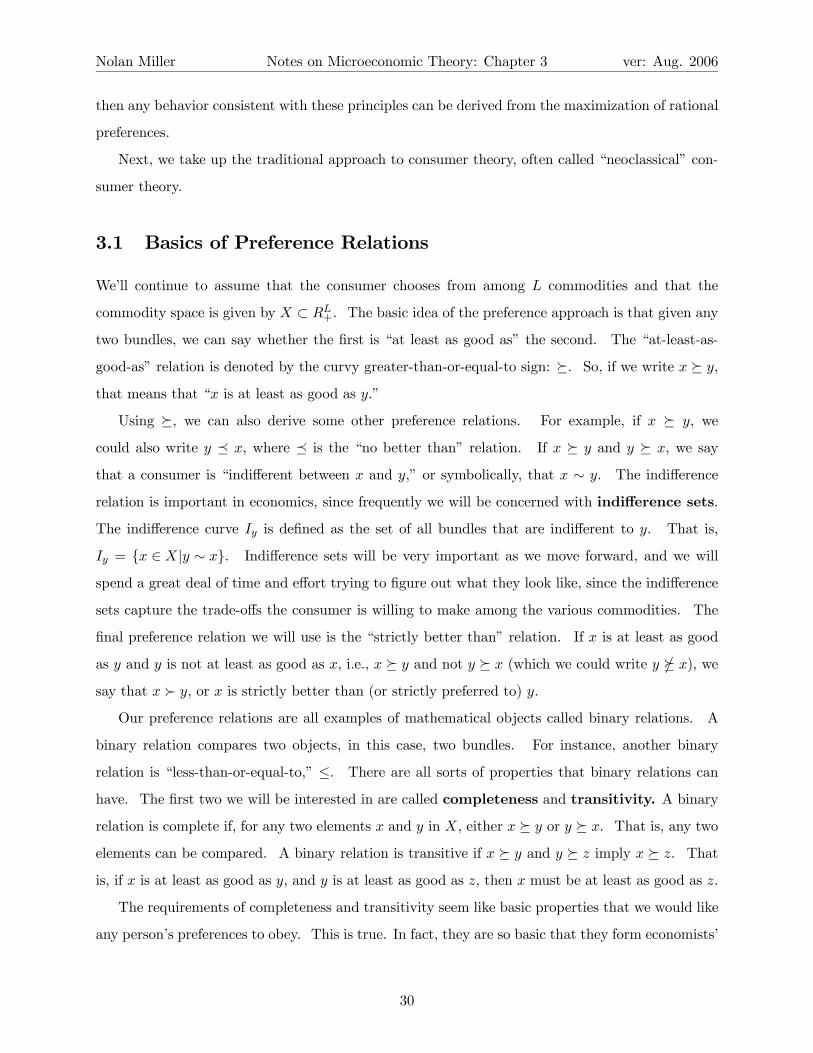
For example, consider a special case of the Cobb-Douglas utility function I mentioned earlier.
u (x1, x2) = x141 x
142 .
Figure 3.4 shows a three-dimensional (3D) graph of this function.3Despite what you are used to, economists always use log to refer to the natural log, ln, since we don’t use base
10 logs at all.
37
Nolan Miller Notes on Microeconomic Theory: Chapter 3 ver: Aug. 2006
0
2
4
6
8
10
x1
0
2
4
6
8
10
x2
0
1
2
3
ux
0
2
4
6
8
10
x1
Figure 3.4: Function u (x)
38

Nolan Miller Notes on Microeconomic Theory: Chapter 3 ver: Aug. 2006
0 2 4 6 8 100
2
4
6
8
10
Figure 3.5: Level sets of u (x)
Notice the curvature of the surface. Now, consider Figure 3.5, which shows the level sets (Ix)
for various utility levels. Notice that the indifference curves of this utility function are convex.
Now, pick an indifference curve. Points offering more utility are located above and to the right of
it. Notice how the contour map corresponds to the 3D utility map. As you move up and to the
right, you move “uphill” on the 3D graph.
Quasiconcavity is a weaker condition than concavity. Concavity is an assumption about how
the numbers assigned to indifference curves change as you move outward from the origin. It says
that the increase in utility associated with an increase in the consumption bundle decreases as
you move away from the origin. As such, it is a cardinal concept. Quasiconcavity is an ordinal
concept. It talks only about the shape of indifference curves, not the numbers assigned to them.
It can be shown that concavity implies quasiconcavity but a function can be quasiconcave without
being concave (can you draw one in two dimensions). It turns out that for the results on utility
39
Nolan Miller Notes on Microeconomic Theory: Chapter 3 ver: Aug. 2006
0
2
4
6
8
10
x1
0
2
4
6
8
10
x2
0
250
500
750
1000
vx
0
2
4
6
8
10
x1
Figure 3.6: Function v (x)
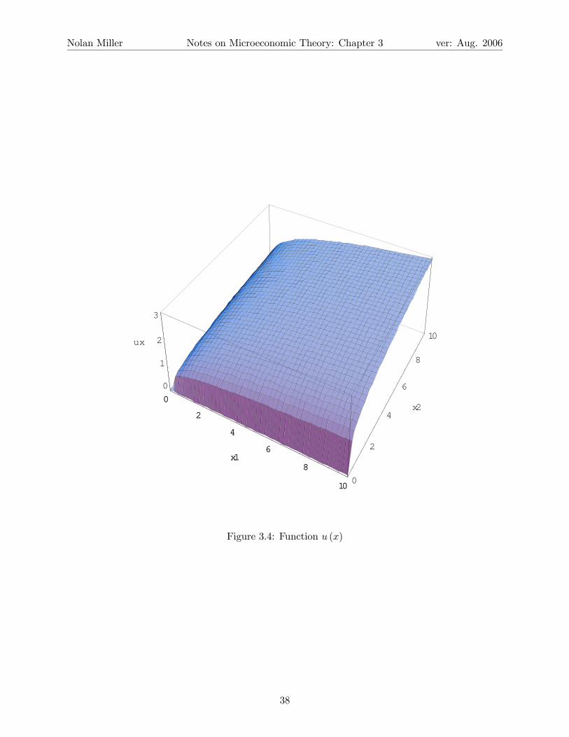
maximization we will develop later, all we really need is quasiconcavity. Since concavity imposes
cardinal restrictions on utility (which is an ordinal concept) and is stronger than we need for our
maximization results, we stick with the weaker assumption of quasiconcavity.4
Here’s an example to help illustrate this point. Consider the following function, which is also
of the Cobb-Douglas form:
v (x) = x321 x
322 .
Figure 3.6 shows the 3D graph for this function. Notice that v (x) is “curved upward” instead of
downward like u (x). In fact, v (x) is a not a concave function, while u (x) is a concave function.5
But, both are quasiconcave. We already saw that u (x) was quasiconcave by looking at its level
4As in the case of convexity and strict convexity, a strictly quasiconcave function is one whose upper level sets are
strictly convex. Thus a function that is quasiconcave but not strictly so can have flat parts on the boundaries of its
indifference curves.5See Simon and Blume or Chiang for good explanations of concavity and convexity in multiple dimensions.
40

Nolan Miller Notes on Microeconomic Theory: Chapter 3 ver: Aug. 2006
0 2 4 6 8 100
2
4
6
8
10
Figure 3.7: Level sets of v (x).
sets.6 To see why v (x) is quasiconcave, let’s look at the level sets of v (x) in Figure 3.7. Even
though v(x) is curved in the other direction, the level sets of v (x) are still convex. Hence v (x) is
quasiconcave. The important point to take away here is that quasiconcavity is about the shape of
level sets, not about the curvature of the 3D graph of the function.
Before going on, let’s do one more thing. Recall u (x) = x141 x
142 and v (x) = x
321 x
322 . Now, consider
the monotonic transformation f (u) = u6. We can rewrite v (x) = x641 x
642 =
µx141 x
142
¶6= f (u (x)).
Hence utility functions u (x) and v (x) actually represent the same preferences! Thus we see that
utility and preferences have to do with the shape of indifference curves, not the numbers assigned
to them. Again, utility is an ordinal, not cardinal, concept.
Now, here’s an example of a function that is not quasiconcave.
h (x) =¡x2 + y2
¢ 14
µ2 +
1
4
³sin³8 arctan
³yx
´´´2¶6That isn’t a proof, just an illustration.
41

Nolan Miller Notes on Microeconomic Theory: Chapter 3 ver: Aug. 2006
2040
6080
100
x120
40
60
80100
x20
10
20utility
2040
6080
100
x1
Figure 3.8: Function h(x)
Don’t worry about where this comes from. Figure 3.8 shows the 3D plot of h (x).
Figure 3.9 shows the isoquants for this utility function. Notice that the level sets are not
convex. Hence, function h (x) is not quasiconcave. After looking at the mathematical analysis of
the consumer’s problem in the next section, we’ll come back to why it is so hard to analyze utility
functions that look like h (x).
3.3 The Utility Maximization Problem (UMP)
Now that we have defined a utility function, we are prepared to develop the model in which
consumers choose the bundle they most prefer from among those available to them.7 In order to
7Notice that in the choice model, we never said why consumers make the choices they do. We only said that
those choices must appear to satisfy homogeneity of degree zero, Walras’ law, and WARP. Now, we say that the
consumer acts to maximize utility with certain properties.
42

Nolan Miller Notes on Microeconomic Theory: Chapter 3 ver: Aug. 2006
0 20 40 60 80 1000
20
40
60
80
100
Figure 3.9: Level Sets of h(x)
43
Nolan Miller Notes on Microeconomic Theory: Chapter 3 ver: Aug. 2006
ensure that the problem is “well-behaved,” we will assume that preferences are rational, continuous,
convex, and locally nonsatiated. These assumptions imply that the consumer has a continuous
utility function u (x), and the consumer’s choices will satisfy Walras’ Law. In order to use calculus
techniques, we will assume that u () is differentiable in each of its arguments. Thus, in other words,
we assume indifference curves have no “kinks.”
The consumer’s problem is to choose the bundle that maximizes utility from among those avail-
able. The set of available bundles is given by the Walrasian budget set Bp,w = {x ∈ X|p · x ≤ w}.
We will assume that all prices are strictly positive (written p >> 0) and that wealth is strictly
positive as well. The consumer’s problem can be written as:
maxx≥0
u (x)
s.t. : p · x ≤ w.
The first question we should ask is: Does this problem have a solution? Since u (x) is a
continuous function and Bp,w is a closed and bounded (i.e., compact) set, the answer is yes by the
Weierstrass theorem - a continuous function on a compact set achieves its maximum. How do
we find the solution? Since this is a constrained maximization problem, we can use Lagrangian
methods. The Lagrangian can be written as:
L = u (x) + λ (w − p · x)
Which implies Kuhn-Tucker first-order conditions (FOC’s):
ui (x∗)− λ∗pi ≤ 0 and xi (ui (x
∗)− λ∗pi) = 0 for i = (1, ..., L)
w − p · x∗ ≥ 0 and λ∗ (w − p · x∗) = 0
Note that the optimal solution is denoted with an asterisk. This is because the first-order conditions
don’t hold everywhere, only at the optimum. Also, note that the value of the Lagrange multiplier
λ is also derived as part of the solution to this problem.
Now, we have a system with L+1 unknowns. So, we need L+1 equations in order to solve for
the optimum. Since preferences are locally non-satiated, we know that the consumer will choose
a consumption bundle that is on the boundary of the budget set. Thus the constraint must bind.
This gives us one equation.
The conditions on xi are complicated because we must allow for the possibility that the consumer
chooses to consume x∗i = 0 for some i at the optimum. This will happen, for example, if the relative
44

Nolan Miller Notes on Microeconomic Theory: Chapter 3 ver: Aug. 2006
price of good i is very high. While this is certainly a possibility, “corner solutions” such as these
are not the focus of the course, so we will assume that x∗i > 0 for all i for most of our discussion.
But, you should be aware of the fact that corner solutions are possible, and if you come across a
corner solution, it may appear to behave strangely.
Generally speaking, we will just assume that solutions are interior. That is, that x∗i > 0 for all
commodities i. In this case, the optimality condition becomes
ui (x∗i )− λ∗pi = 0. (3.1)
Solving this equation for λ∗ and doing the same for good j yields:
− ui (x∗i )
uj
³x∗j
´ = − pipjfor all i, j ∈ {1, ..., L} .
This turns out to be an important condition in economics. The condition on the right is the
slope of the budget line, projected into the i and j dimensions. For example, if there are two
commodities, then the budget line can be written x2 = −p1p2x1 +
wp2. The left side, on the other
hand, is the slope of the utility indifference curve (also called an isoquant or isoutility curve).
To see why − ui(x∗i )uj(x∗j)
is the slope of the isoquant, consider the following identity: u (x1, x2 (x1)) ≡ k,
where k is an arbitrary utility level and x2 (x1) is defined as the level of x2 needed to guarantee
the consumer utility k when the level of commodity 1 consumed is x1. Differentiate this identity
with respect to x1:8
u1 + u2dx2dx1
= 0
dx2dx1
= −u1u2
So, at any point (x1, x2), −u1(x1,x2)u2(x1,x2)
is the slope of the implicitly defined curve x2 (x1) . But, this
curve is exactly the set of points that give the consumer utility k, which is just the indifference
curve. As mentioned earlier, we call the slope of the indifference curve the marginal rate of
substitution (MRS): MRS = −u1u2.
Thus the optimality condition is that at the optimal consumption bundle, the MRS (the rate
that the consumer is willing to trade good x2 for good x1, holding utility constant) must equal the
ratio of the prices of the two goods. In other words, the slope of the utility isoquant is the same
as the slope of the budget line. Combine this with the requirement that the optimal bundle be on
8Here, we adopt the common practice of using subscripts to denote partial derivatives, ∂u(x)∂xi= ui.
45

Nolan Miller Notes on Microeconomic Theory: Chapter 3 ver: Aug. 2006
x*
x1
x2
Utility increases
Budget set
Figure 3.10: Tangency Condition
the budget line, and this implies that the utility isoquant will be tangent to the budget line at the
optimum.
In Figure 3.10, x∗ is found at the point of tangency between the budget set and one of the
utility isoquants. Notice that because the level sets are convex, there is only one such point. If
the level sets were not convex, this might not be the case. Consider, for example, Figure 3.9.
Here, for any budget set, there will be many points of tangency between utility isoquants and the
budget set. Some will be maximizers, and some won’t. The only way to find out whether a
point is a maximizer is to go through the long and unpleasant process of checking the second-order
conditions. Further, even once a maximizer is found, it may behave strangely. We discuss this
point further in Section 3.3.1 below.
So, we are looking for the point of tangency between the budget set and a utility isoquant. One
way to do this would be to use the following procedure:
1. Choose a point on the budget line, call it z. Find its upper level set Uz. Find Uz ∩ Bp,w.
This gives you the set of points that are feasible and at least as good as z.
2. If this set contains only z, you are done: z is the utility maximizing point. If this set contains
more than just z, choose an arbitrary point on the budget line that is also inside Uz and
repeat the process. Keep going until the only point that is in both the upper level set and
the budget set is that point itself. This point is the optimum.
46

Nolan Miller Notes on Microeconomic Theory: Chapter 3 ver: Aug. 2006
The problem with this procedure is that it could potentially take a very long time to find the
optimal point. The calculus approach allows us to do it much faster by finding the point along
the budget line that has the same slope as the indifference curve. This is a much easier task, but
it turns out that it is really just a shortcut for the procedure outlined above.
3.3.1 Walrasian Demand Functions and Their Properties
So, suppose that we have found the utility maximizing point, x∗. What have we really found?
Notice that if the prices and wealth were different, the utility maximizing point would have been
different. For this reason, we will write the endogenous variable x∗ as a function of prices and
wealth, x (p,w) = (x1 (p,w) , x2 (p,w) ..., xL (p,w)). This function gives the utility maximizing
bundle for any values of p and w. We will call x (p,w) the consumer’s Walrasian demand
function, although it is also sometimes called the Marshallian or ordinary demand function. This
is to distinguish it from another type of demand function that we will study later.
As a consequence of what we have done, we can immediately derive some properties of the
Walrasian demand function:
1. Walras’ Law: p ·x (p,w) ≡ w for all p and w. This follows from local nonsatiation. Recall
the definition of local non-satiation: For any x ∈ X and ε > 0 there exists a y ∈ X such
that ||x− y|| < ε and y  x. Thus the only way for x to be the most preferred bundle is if
there the nearby point that is better is not in the budget set. But, this can only happen if
x satisfies p · x (p,w) ≡ w.
2. Homogeneity of degree zero in (p,w) . The definition of homogeneity is the same as
always. x (αp, αw) = x (p,w) for all p,w and α > 0. Just as in the choice based approach,
the budget set does not change: Bp,w = Bαp,αw. Now consider the first-order condition:
− ui (x∗i )
uj
³x∗j
´ = −pipjfor all i, j ∈ {1, ..., L} .
Suppose we multiply all prices by α > 0. This makes the right hand side −αpiαpj
= − pipj,
which is just the same as before. So, since neither the budget constraint nor the optimality
condition are changed, the optimal solution must not change either.
3. Convexity of x (p,w). Up until now we have been assuming that x (p,w) is a unique point.
However, it need not be. For example, if preferences are convex but not strictly convex, the
47

Nolan Miller Notes on Microeconomic Theory: Chapter 3 ver: Aug. 2006
isoquants will have flat parts. If the budget line has the same slope as the flat part, an entire
region may be optimal. However, we can say that if preferences are convex, the optimal
region will be a convex set. Further, we can add that if preferences are strictly convex, so
that u () is strictly quasiconcave, then x (p,w) will be a single point for any (p,w). This is
because strict quasiconcavity rules out flat parts on the indifference curve.
A Note on Optimization: Necessary Conditions and Sufficient Conditions
Notice that we derived the first-order conditions for an optimum above. However, while these
conditions are necessary for an optimum, they are not generally sufficient - there may be points
that satisfy them that are not maxima. This is a technical problem that we don’t really want to
worry about here. To get around it, we will assume that utility is quasiconcave and monotone
(and some other technical conditions that I won’t even mention). In this case we know that the
first-order conditions are sufficient for a maximum.
In most courses in microeconomic theory, you would be very worried about making sure that the
point that satisfies the first-order conditions is actually a maximizer. In order to do this you need
to check the second order conditions (make sure the function is “curved down”). This is a long
and tedious process, and, fortunately, the standard assumptions we will make, strict quasiconcavity
and monotonicity, are enough to make sure that any point that satisfies the first-order conditions
is a maximizer (at least when the constraint is linear). Still, you should be aware that there is
such things as second-order conditions, and that you either need to check to make sure they are
satisfied or make assumptions to ensure that they are satisfied. We will do the latter, and leave
the former to people who are going to be doing research in microeconomic theory.
A Word on Nonconvexities
It is worthwhile to spend another moment on what can happen if preferences are not convex, i.e.
utility is not quasiconcave. We already mentioned that with nonconvex preferences it becomes
necessary to check second-order conditions to determine if a point satisfying the first-order condi-
tions is really a maximizer. There can also be other complications. Consider a utility function
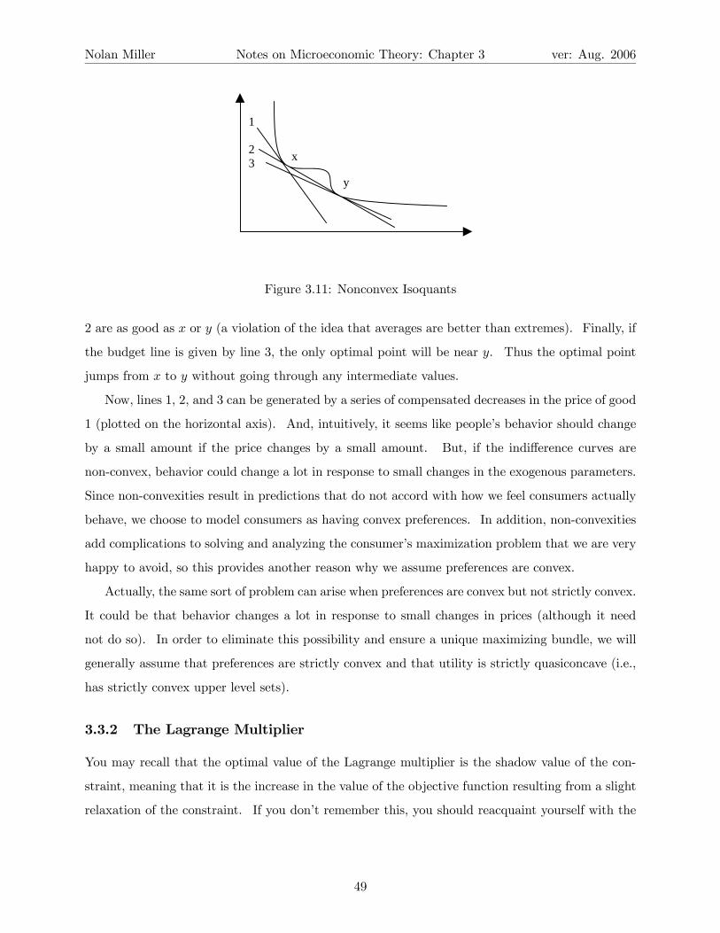
where the isoquants are not convex, shown in Figure 3.11.
When the budget line is given by line 1, the optimal point will be near x. When the budget line
is line 2, the optimal points will be either x or y. But, none of the points between x and y on line
48
Nolan Miller Notes on Microeconomic Theory: Chapter 3 ver: Aug. 2006
x
y
1
23
Figure 3.11: Nonconvex Isoquants
2 are as good as x or y (a violation of the idea that averages are better than extremes). Finally, if
the budget line is given by line 3, the only optimal point will be near y. Thus the optimal point
jumps from x to y without going through any intermediate values.
Now, lines 1, 2, and 3 can be generated by a series of compensated decreases in the price of good
1 (plotted on the horizontal axis). And, intuitively, it seems like people’s behavior should change
by a small amount if the price changes by a small amount. But, if the indifference curves are
non-convex, behavior could change a lot in response to small changes in the exogenous parameters.
Since non-convexities result in predictions that do not accord with how we feel consumers actually
behave, we choose to model consumers as having convex preferences. In addition, non-convexities
add complications to solving and analyzing the consumer’s maximization problem that we are very
happy to avoid, so this provides another reason why we assume preferences are convex.
Actually, the same sort of problem can arise when preferences are convex but not strictly convex.
It could be that behavior changes a lot in response to small changes in prices (although it need
not do so). In order to eliminate this possibility and ensure a unique maximizing bundle, we will
generally assume that preferences are strictly convex and that utility is strictly quasiconcave (i.e.,
has strictly convex upper level sets).
3.3.2 The Lagrange Multiplier
You may recall that the optimal value of the Lagrange multiplier is the shadow value of the con-
straint, meaning that it is the increase in the value of the objective function resulting from a slight
relaxation of the constraint. If you don’t remember this, you should reacquaint yourself with the
49

Nolan Miller Notes on Microeconomic Theory: Chapter 3 ver: Aug. 2006
point by looking in the math appendix of your favorite micro text or “math for economists” book.9
If you still don’t believe this is true, I present you with the following derivation. In addition to
showing this fact about the value of λ∗, it also illustrates a common method of proof in economics.
Consider the utility function u (x). If we substitute in the demand functions, we get
u (x (p,w))
which is the utility achieved by the consumer when she chooses the best bundle she can at prices
p and wealth w. The constraint in the problem is:
p · x ≤ w.
So, relaxing the constraint means increasing w by a small amount. If this is unfamiliar to you,
think about why it is so: The budget set Bp,w+dw strictly includes the budget set Bp,w, and so
any bundle that could be chosen before the wealth increase could also be chosen after. Since there
are more feasible points, the constraint after the wealth increase is a relaxation of the constraint
before. We can analyze the effect of this by differentiating u (x (p,w)) with respect to w :
d
dwu (x (p,w)) =
LXi=1
duidxi
dxidw
=LXi=1
λpidxidw
= λLXi=1
pidxidw
= λ.
The transition from the first line to the second line is accomplished by substituting in the first-order
condition: duidxi− λpi = 0. The transition from the second line to the third line is trivial (you can
factor out λ since it is a constant). The transition from the third line to the fourth line comes from
the comparative statics of Walras’ Law that we derived in the choice section. Since p ·x (p,w) ≡ w,Ppi
dxldw = 1 (you could rederive this by differentiating the identity with respect to w if you want).
3.3.3 The Indirect Utility Function and Its Properties
The Walrasian demand function x (p,w) gives the commodity bundle that maximizes utility subject
to the budget constraint. If we substitute this bundle into the utility function, we get the utility
9 If you don’t have a favorite, I recommend “Mathematics for Economists” by Simon and Blume.
50
Nolan Miller Notes on Microeconomic Theory: Chapter 3 ver: Aug. 2006
that is earned when the consumer chooses the bundle that maximizes utility when prices are p and
wealth is w. That is, define the function v (p,w) as:
v (p,w) ≡ u (x (p,w)) .
We call v (p,w) the indirect utility function. It is indirect because while utility is a function
of the commodity bundle consumed, x, indirect utility function v (p,w) is a function of p and w.
Thus it is indirect because it tells you utility as a function of prices and wealth, not as a function
of commodities. You can think of it this way. Given prices p and wealth w, x (p,w) is the
commodity bundle chosen and v (p,w) is the utility that results from consuming x (p,w). But, if I
know v (p,w), then given any prices and wealth I can calculate utility without first having to solve
for x (p,w).
Just as x (p,w) had certain properties, so does v (p,w). In fact, most of them are inherited
from the properties of x (p,w). Suppose that preferences are locally nonsatiated. The indirect
utility function corresponding to these preferences v (p,w) has the following properties:
1. Homogeneity of degree zero: Since x (p,w) = x (αp, αw) for α > 0,
v (αp, αw) = u (x (αp, αw)) = u (x (p,w)) = v (p,w) .
In other words, since the bundle you consume doesn’t change when you scale all prices and
wealth by the same amount, neither does the utility you earn.
2. v (p,w) is strictly increasing in w and non-increasing in pl. If xl > 0, v (p,w) is strictly
decreasing in pl. Indirect utility is strictly increasing in w by local non-satiation. If x (p,w)
is optimal and preferences are locally non-satiated, there must be a point just on the other side
of the budget line that the consumer strictly prefers. If w increases a little bit, this point will
become feasible, and the consumer will earn higher utility. Indirect utility is non-increasing
in pl since an increase in pl shrinks the feasible region. After pl increases, the budget line lies
inside of the old budget set. Since the consumer could have chosen these points but didn’t,
the consumer can be no better off than before the price increase. Note that the consumer
will do strictly worse unless it is the case that xl (p,w) = 0 and the consumer still chooses to
consume xl = 0 after the price increase. In this case, the consumer’s consumption bundle
does not change, so neither does her utility. This is a subtle point having to do with corner
solutions. But, a carefully drawn picture should make it all clear (See Figure 3.12).
51

Nolan Miller Notes on Microeconomic Theory: Chapter 3 ver: Aug. 2006
Utility increases
x1
x2
Price changes
Figure 3.12: V (p,w) is decreasing in p
3. v (p,w) is quasiconvex in (p,w). In other words, the set {(p,w) |v (p,w) ≤ v} is convex for
all v. Consider two distinct price-wealth vectors (p0, w0) and (p00, w00) such that v (p0, w0) =
v (p00, w00). Since the consumer chooses her most preferred consumption bundle at each price,
x(p0, w0) is preferred to all other bundles in Bp0,w0 and x(p00, w00) is preferred to all other
bundles in Bp00,w00 . Now, consider the budget set formed at an average price pa = ap0 + ap00
and wealth wa = aw0 + (1− a)w00. Every bundle in Bpa,wa will lie within either Bp0,w0 or
Bp00,w00 . Hence the utility of any bundle in Bpa,wa can be no larger than the utility of the
chosen bundle, v(p0, w). Thus v(p0, w) ≥ v(pa, w), which proves the result. Note: see the
diagram on page 57 of MWG.10 A question for you: What is the intuitive meaning of this?
4. v (p,w) is continuous in p and w. Small changes in p and w result in small changes in
utility. This is especially clear in the case where indifference curves are strictly convex and
differentiable.
3.3.4 Roy’s Identity
Consider the indirect utility function: v (p,w) = maxx∈Bp,w u (x). The function v (p,w) tells you
how much utility the consumer earns when prices are p and wealth is w. Thanks to a very clever
bit of mathematics, we can exploit this in order to figure out the relationship between the indirect
utility function and the demand functions x (p,w).
10This is a slightly informal argument. Formally, we must show for any (p0, w0) and (p00, w00), v (pa, wa) ≤
max {v (p0, w0) , v (p00, w00)}. But, the same intuition continues to hold.
52

Nolan Miller Notes on Microeconomic Theory: Chapter 3 ver: Aug. 2006
The definition of the indirect utility function implies that the following identity is true:
v (p,w) ≡ u (x (p,w)) .
Differentiate both sides with respect to pl :
∂v
∂pl=
LXi=1
∂u
∂xi
∂xi∂pl
.
But, based on the first-order conditions for utility maximization, which we know hold when u () is
evaluated at the optimal x, x (p,w) (see equation (3.1)):
∂u
∂xi= λpi.
And, we also know (from Section 3.3.2) that the Lagrange multiplier is the shadow price of the
constraint: λ = ∂v∂w . Hence:
∂v
∂pl=
LXi=1
∂u
∂xi
∂xi∂pl
=LXi=1
λpi∂xi∂pl
= λLXi=1
pi∂xi∂pl
=∂v
∂w
LXi=1
pi∂xi∂pl
.
Now, recall the comparative statics result of Walras’ Law with respect to a change in pl :
xl (p,w) = −LXi=1
pi∂xi∂pl
.
Substituting this in yields:
∂v
∂pl= − ∂v
∂wxl (p,w)
xl (p,w) = −∂v∂pl∂v∂w
.
The last equation, known as Roy’s identity, allows us to derive the demand functions from the
indirect utility function. This is useful because in many cases it will be easier to estimate an
indirect utility function and derive the direct demand functions via Roy’s identity than to derive
x (p,w) directly. Estimating Roy’s identity involves estimating a single equation. Estimating
x (p,w), on the other hand, amounts to finding for every value of p and w the solution to a set of
L+ 1 first-order equations, which themselves may have unknown parameters.
53

Nolan Miller Notes on Microeconomic Theory: Chapter 3 ver: Aug. 2006
3.3.5 The Indirect Utility Function and Welfare Evaluation
Consider the situation where the price of good 1 increases from p1 to p01. What is the impact
of this price change on the consumer? One way to measure it is in terms of the indirect utility
function:
impact = v¡p0, w
¢− v (p,w) .
That is, the impact of the price change is equal to the difference in the consumer’s utility at prices p0
and p. While this is certainly a measure of the impact of the price change, it is essentially useless.
There are a number of reasons why, but they all hinge on the fact that utility is an ordinal, not a
cardinal concept. As you recall, the only meaning of the numbers assigned to bundles by the utility
function is that x  y if and only if u (x) > u (y). In particular, if u (x) = 2u (y), this does not mean
that the consumer likes bundle x twice as much as bundle y. Also, if u (x)− u (z) > u (s)− u (t),
this doesn’t mean that the consumer would rather switch from bundle z to x than from t to s.
Because of this, there is really nothing we can make of the numerical value of v (p0, w) − v (p,w).
The only thing we can say is that if this difference is positive, the consumer likes (p0, w) more than
(p,w). But, we can’t say how much more.
Another problem with using the change in the indirect utility function as a measure of the
impact of a policy change is that it cannot be compared across consumers. Comparing the change
in two different utility functions is even more meaningless than comparing the change in a single
person’s utility function. This is because even if both utility functions were cardinal measures of
the benefit to a consumer (which they aren’t), there would still be no way to compare the scales
of the two utility functions. This is the “problem of interpersonal comparison of utility,” which
arises in many aspects of welfare economics.
As a possible solution to the problem, consider the following thought experiment. Initially,
prices and wealth are given by (p,w). I am interested in measuring the impact of a change in prices
to p0. So, I ask you the following question: By how much would I have to change your wealth so
that you are indifferent between (p0, w) and (p,w0)? That is, for what value w0 does
v¡p0, w
¢= v
¡p,w0
¢.
The change in wealth, w0 − w, in essence gives a monetary value for the impact of this change in
price. And, this monetary value is a better measure of the impact of the price change than the
utility measurement, because it is, at least to a certain extent, comparable.11 You can compare11 I say to a certain extent, because the value of an additional ∆w dollars of wealth will depend on the initial state.
54

Nolan Miller Notes on Microeconomic Theory: Chapter 3 ver: Aug. 2006
the impact of two different changes in prices by looking at the associated changes in wealth needed
to compensate the consumer. Similarly, you can compare the impact of price changes on different
consumers by comparing the changes in wealth necessary to leave them just as well off.12
Finally, although using the amount of money needed to compensate the consumer is an imperfect
measure of the impact of a policy decision, it has one huge benefit for the neoclassical economist,
and that is that it is observable, at least in principle. There is nothing we can do to observe utility
scales. However, we can often elicit from people the amount of money they would find equivalent
to a certain policy change, either through experiments, surveys, or other estimation techniques.
3.4 The Expenditure Minimization Problem (EMP)
In the previous section, I argued that a good measure of the impact of a change in prices was the
change in wealth necessary to make the consumer as well off at the old prices and new wealth as
she was at the new prices and old wealth. However, this is not an easy exercise when all you have
to work with is the indirect utility function. If we had a function that tells you how much wealth
you would need to have in order to achieve a certain level of utility, then we would be able to do
this much more efficiently. There is such a function. It is called the expenditure function, and
in this section we will develop it.
The expenditure minimization problem (EMP) asks the question, if prices are p, what is
the minimum amount the consumer would have to spend to achieve utility level u? That is:
minx
p · x
s.t. : u (x) ≥ u.
Before we go on, let’s take a moment to figure out what the endogenous and exogenous variables
are here. The exogenous variables are prices p and the reservation (or target) utility level u. The
endogenous variable is x, the consumption bundle. So, in words, the expenditure minimization
bundle amounts to finding the bundle x that minimizes the cost of achieving utility u when prices
are p.
The Lagrangian for this problem is given by:
LEMP = p · x− λ (u (x)− u) .
For instance, poor people presumably value the same wealth increment more than rich people.12Again, this measure is imperfect because it assumes that the two consumers have the same marginal utility of
wealth.
55
Nolan Miller Notes on Microeconomic Theory: Chapter 3 ver: Aug. 2006
Assuming an interior solution, the first-order conditions are given by:13
pi − λui (x) = 0 for i ∈ {1, ..., L} (3.2)
λ (u (x)− u) = 0
If u () is well behaved (e.g., quasiconcave and increasing in each of its arguments), then the con-
straint will bind, and the second condition can be written as u (x) = u. Further, a unique solution
to this problem will exist for any values of p and u. We will denote the value of the solution
to this problem by h (p, u) ∈ X. That is, h (p, u) is an L dimensional vector whose lth compo-
nent, hl (p, u) gives the amount of commodity l that is consumed when the consumer minimizes
the cost of achieving utility u at prices p. The function h (p, u) is known as the Hicksian (or
compensated) demand function.14 It is a demand function because it specifies a consumption
bundle. It differs from the Walrasian (or ordinary) demand function in that it takes p and u as its
arguments, whereas the Walrasian demand function takes p and w as its arguments.
In other words, h (p, u) and x (p,w) are the answers to two different but related problems.
Function x (p,w) answers the question, “Which commodity bundle maximizes utility when prices are
p and wealth is w?” Function h (p, u) answers the question, “Which commodity bundle minimizes
the cost of attaining utility u when prices are p?” We’ll return to the difference between the two
types of demand shortly.
Since h (p, u) solves the EMP, substitution of h (p, u) into the first-order conditions for the EMP
yields the identities (assuming the constraint binds):
pi − λui (h (p, u)) ≡ 0 for i ∈ {1, ..., L}
u (h (p, u))− u ≡ 0
Further, just as we defined the indirect utility function as the value of the objective function of
the UMP, u (x), evaluated at the optimal consumption bundle, x (p,w), we can also define such a
function for the EMP. The expenditure function, denoted e (p, u), is defined by:
e (p, u) ≡ p · h (p, u)
and is equal to the minimum cost of achieving utility u, for any given p and u.
13Again, remember that if f (y) is a function with a vector y as its argument, the notation fi will frequently be
used as shorthand notation for ∂f∂yi. Thus ui denotes ∂u
∂xi.
14We’ll return to why h (p, u) is called the compensated demand function in a while.
56

Nolan Miller Notes on Microeconomic Theory: Chapter 3 ver: Aug. 2006
3.4.1 A First Note on Duality
Consider the first-order conditions (from (3.2)) for xi and xj . Solving each for λ yields:
piui
= λ =pjuj
uiuj
=pipj. (3.3)
Recall that this is the same tangency condition we derived in the UMP. What does this mean?
Consider a price vector p and wealth w. The bundle that solves the UMP, x∗ = x (p,w) is found at
the point of tangency between the budget line and the consumer’s utility isoquant. The consumer’s
utility at this point is given by u∗ = u (x∗). Thus x∗ is the point of tangency between the line
p · x = w and the curve u (x) = x∗.
Now, consider the EMP when the target utility level is given by u∗. The bundle that solves
the EMP is the bundle that achieves utility u∗ at minimum cost. This is located by finding the
point of tangency between the curve u (x) = u∗ and a budget line (which is what (3.3) says). But,
we already know from the UMP that the curve u (x) = u∗ is tangent to the budget line p · x = w
at x∗ (and is tangent to no other budget line). Hence x∗ must solve the EMP problem when the
target utility level is u∗! Further, since x∗ lies on the budget line, p · x∗ = w. So the minimum
cost of achieving utility u∗ is w. Thus the UMP and the EMP pick out the same point.
Let me restate what I’ve just argued. If x∗ solves the UMP when prices are p and wealth is w,
then x∗ solves the EMP when prices are p and the target utility level is u (x∗). Further, maximal
utility in the UMP is u (x∗) and minimum expenditure in the EMP is w. This result is called the
“duality” of the EMP and the UMP.
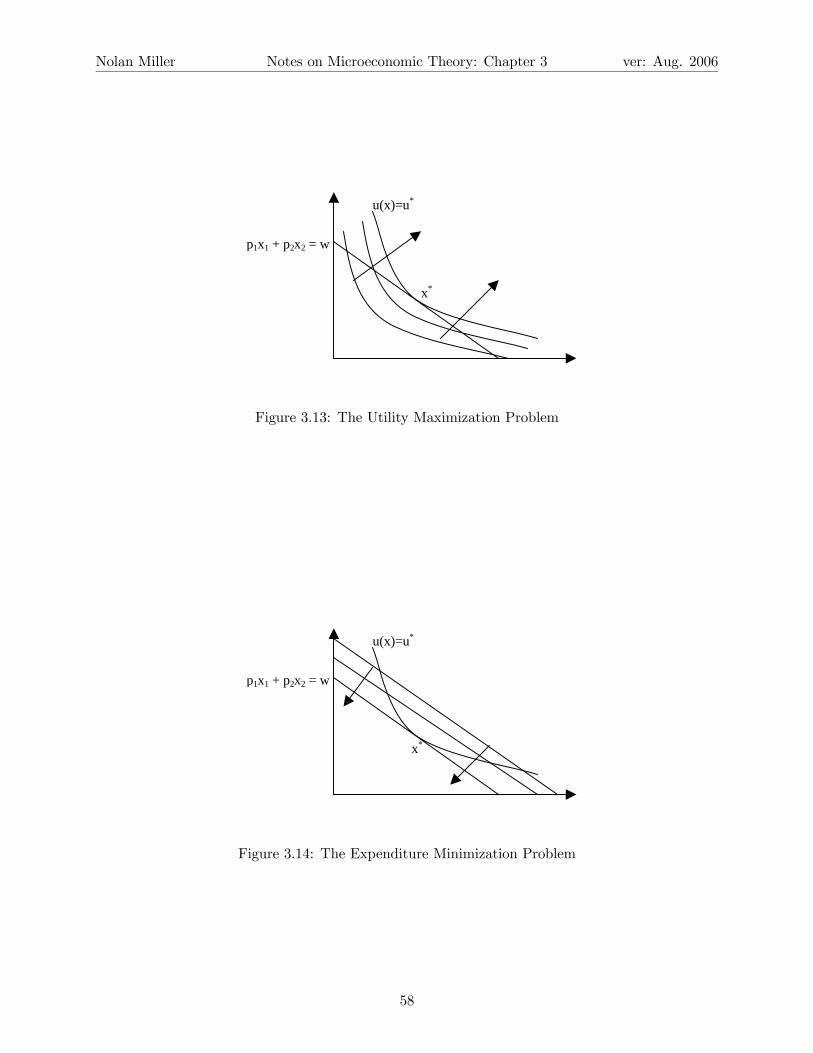
The UMP and the EMP are considered dual problems because the constraint in the UMP is
the objective function in the EMP and vice versa. This is illustrated by looking at the graphical
solutions to the two problems. In the UMP, shown in Figure 3.13, you keep increasing utility until
you find the one that is tangent to the budget line.In the EMP, on the other hand, shown in Figure
3.14, you keep decreasing expenditure (which is like shifting a budget line toward the origin) until
you find the expenditure line that is tangent to u (x) = u∗. Although the process of finding the
optimal point is different in the UMP and EMP, they both pick out the same point because they
are looking for the same basic relationship, as expressed in equation (3.3).
The duality relationship between the EMP and the UMP is captured by the following identities,
57
Nolan Miller Notes on Microeconomic Theory: Chapter 3 ver: Aug. 2006
x*
p1x1 + p2x2 = w
u(x)=u*
Figure 3.13: The Utility Maximization Problem
x*
p1x1 + p2x2 = w
u(x)=u*
Figure 3.14: The Expenditure Minimization Problem
58
Nolan Miller Notes on Microeconomic Theory: Chapter 3 ver: Aug. 2006
to which we will return later:
h (p, v (p,w)) ≡ x (p,w)
x (p, e (p, u)) ≡ h (p, u) .
These identities restate the principles discussed previously. The first says that the commodity
bundle that minimizes the cost of achieving the maximum utility you can achieve when prices are
p and wealth is w is the bundle that maximizes utility when prices are p and wealth is w. The
second says that the bundle that maximizes utility when prices are p and wealth is equal to the
minimum amount of wealth needed to achieve utility u at those prices is the same as the bundle
that minimizes the cost of achieving utility u when prices are p.
Similar identities can be written using the indirect utility function and expenditure function:
u ≡ v (p, e (p, u))
w ≡ e (p, v (p,w)) .
Note to MWG readers: There is a mistake in Figure 3.G.3. The relationships on
the horizontal line connecting v (p,w) and e (p, u) should be the ones written directly
above.
The main implication of the previous analysis is this: The expenditure function contains the
exact same information as the indirect utility function. And, since the indirect utility function can
be used (by Roy’s identity) to derive the Walrasian demand functions, which can, in turn, be used
to recover preferences, the expenditure function contains the exact same information as
the utility function. This means that if you know the consumer’s expenditure function, you
know her utility function, and vice versa. No information is lost along the way. This is another
expression of what people mean when they say that the UMP and EMP are dual problems - they
contain exactly the same information.
3.4.2 Properties of the Hicksian Demand Functions and Expenditure Function
In this section, we refer both to function u (x) and to a particular level of utility, u. In order to be
clear, let’s put a bar over the u when we are talking about a level of utility, i.e., u. Just as we derived
the properties of x (p,w) and v (p,w), we can also derive the properties of the Hicksian demand
functions h (p, u) and expenditure function e (p, u). Let’s begin with h (p, u) . We will assume that
u () is a continuous utility function representing a locally non-satiated preference relation.
59

Nolan Miller Notes on Microeconomic Theory: Chapter 3 ver: Aug. 2006
Properties of the Hicksian Demand Functions
The Hicksian demand functions have the following properties:
1. Homogeneity of degree zero in p : h (αp, u) ≡ h (p, u) for p, u, and α > 0. NOTE: THIS IS
HOMOGENEITY IN P , NOT HOMOGENEITY IN P AND U ! Homogeneity of degree zero
is best understood in terms of the graphical presentation of the EMP. The solution to the
EMP is the point of tangency between the utility isoquant u (x) = u and one of the budget
lines. This is determined by the slope of the expenditure lines (lines of the form p · x = k,
where k is any constant). Any change that doesn’t affect the slope of the budget lines should
not affect the cost-minimizing bundle (although it will affect the expenditure on the cost
minimizing bundle). Since the slope of the expenditure line is determined by relative prices
and since scaling all prices by the same amount does not affect relative prices, the solution
should not change. More formally, the EMP at prices αp is
minx
αp · x
s.t. : u (x) ≥ u.
But, this problem is formally equivalent to:
minα (p · x) : s.t. : u (x) ≥ x
which is equivalent to:
αminx
p · x : s.t. : u (x) ≥ x
which is just the same as the EMP when prices are p, except that total expenditure is
multiplied by α, which doesn’t affect the cost minimizing bundle.
2. No excess utility: u (h (p, u)) = u. This follows from the continuity of u (). Suppose
u (h (p, u)) > u. Then consider a bundle h0 that is slightly smaller than h (p, u) on all
dimensions. By continuity, if h0 is sufficiently close to h (p, u), then u (h0) > u as well. But,
then h0 is a bundle that achieves utility u at lower cost than h (p, u), which contradicts the
assumption that h (p, u) was the cost minimizing bundle in the first place.15 From this we
can conclude that the constraint always binds in the EMP.15This type of argument - called “Proof by Contradiction” - is quite common in economics. If you want to show
a implies b, assume that b is false and show that if b is false then a must be false as well. Since a is assumed to be
true, this implies that b must be true as well.
60

Nolan Miller Notes on Microeconomic Theory: Chapter 3 ver: Aug. 2006
3. If preferences are convex, then h (p, u) is a convex set. If preferences are strictly convex (i.e.
u () is strictly quasiconcave), then h (p, u) is single valued.
Properties of the Expenditure Function
Based on the properties of h (p, u), we can derive properties of the expenditure function, e (p, u).
1. Function e (p, u) is homogeneous of degree one in p: Since h (p, u) is homogeneous of
degree zero in p, this means that scaling all prices by α > 0 does not affect the bundle
demanded. Applying this to total expenditure:
e (αp, u) = αp · h (αp, u) = αp · h (p, u) = αe (p, u) .
In words, if all prices change by a factor of α, the same bundle as before achieves utility level
u at minimum cost, only it now costs you twice as much as it used to. This is exactly what
it means for a function to be homogeneous of degree one.
2. Function e (p, u) is strictly increasing in u and non-decreasing in pl for any l. I’ll
give the argument here to show that e (p, u) cannot be decreasing in u. There are a few
more details to show that it cannot stay constant either, but most of the intuition of the
argument is contained in showing that e (p, u) cannot be strictly decreasing. The argu-
ment is by contradiction. Suppose that for u0 > u, e (p, u) > e (p, u0). But, then h (p, u0)
satisfies the constraint u (x) ≥ u and does so at lower cost than h (p, u), which contra-
dicts the assumption that h (p, u) is the cost minimizing bundle that achieves utility level u.
The argument that e (p, u) is nondecreasing in pl uses another method which is quite common,
a method I call “feasible but not optimal.” Let p and p0 differ only in component l, and let
p0l > pl. From the definition of the expenditure function, e (p0, u) = p0 ·h (p0, u) ≥ p·h (p0, u) ≥
e (p, u). The first equality follows from the definition of the expenditure function, the first
≥ follows from the fact that p0 > p (note: p0 · h (p0, u) > p · h (p, u) if hl (p0, u) > 0), and the
second ≥ follows from the fact that h (p0, u) achieves utility level u but does not necessarily
do so at minimum cost (i.e. h (p0, u) is feasible in the EMP for (p, u) but not necessarily
optimal).
3. Function e (p, u) is concave in p.16 Consider two price vectors p and p0, and let pa =
16Recall the definition of concavity. Consider y and y0 such that y 6= y0. Function f (y) is concave if, for any
a ∈ [0, 1], f (ay + (1− a) y0) ≥ af (y) + (1− a) f (y0).
61

Nolan Miller Notes on Microeconomic Theory: Chapter 3 ver: Aug. 2006
ap+ (1− a) p0.
e (pa, u) = pa · h (pa, u)
= ap · h (pa, u) + (1− a) p · h (pa, u)
≥ ap · h (p, u) + (1− a) p0 · h¡p0, u
¢where the first line is the definition of e (p, u), the second follows from the definition of pa,
and the third follows from the fact that h (pa, u) is feasible but not optimal in the EMP for
(p, u) and (p0, u).
The following heuristic explanation is also helpful in understanding the concavity of e (p, u).
Suppose prices change from p to p0. If the consumer continued to consume the same bundle at the
old prices, expenditure would increase linearly:
∆expenditure =¡p0 − p
¢· h (p, u) .
But, in general the consumer will not continue to consume the same bundle after the price change.
Rather, he will rearrange his bundle in order to minimize the cost of achieving u at the new prices,
p0. Since this will save the consumer some money, total expenditure will decrease at less than a
linear rate. And, an alternate definition of concavity is that the function always increases at less
than a linear rate. In other words, f (x) is concave if it always lies below its tangent lines.17
3.4.3 The Relationship Between the Expenditure Function and Hicksian De-
mand
Just as there was a relationship between the indirect utility function v (p,w) and the Walrasian
demand functions x (p,w), there is also a relationship between the expenditure function e (p, u)
and the Hicksian demand function h (p, u). In fact, it is even more straightforward for e (p, u) and
h (p, u). Let’s start with the derivation
e (p, u) ≡ p · h (p, u)
Since this is an identity, differentiate it with respect to pi:
∂e
∂pi≡ hi (p, u) +
Xj
pj∂hj∂pi
.
17This explanation will be clearer once we show that hl (p, u) =∂e(p,u)∂pl
, i.e. that hl (p, u) is exactly the rate of
increase in expenditure if pl increases by a small amount. Thus e (p0, u)− e (p, u) ≤ h (p, u) · (p0 − p) is exactly the
definition of concavity.
62
Nolan Miller Notes on Microeconomic Theory: Chapter 3 ver: Aug. 2006
Now, substitute in the first-order conditions, pj = λuj
∂e
∂pi≡ hi (p, u) + λ
Xj
uj∂hj∂pi
. (3.4)
Since the constraint binds at any optimum of the EMP,
u (h (p, u)) ≡ u
Differentiate with respect to pi : Xj
uj∂hj∂pi
= 0
and substituting this into (3.4) yields:
∂e
∂pj≡ hj (p, u) . (3.5)
That is, the derivative of the expenditure function with respect to pj is just the Hicksian demand
for commodity j.
The importance of this result is similar to the importance of Roy’s identity. Frequently, it
will be easier to measure the expenditure function than the Hicksian demand function. Since
we are able to derive the Hicksian demand function from the expenditure function, we can derive
something that is hard to observe from something that is easier to observe.
From (3.5) we can derive several additional properties (assuming u () is strictly quasiconcave
and h () is differentiable):
1. (a) ∂hi∂pj
= ∂2e∂pi∂pj
. This one follows directly from the fact that (3.5) is an identity. Let
Dph (p, u) be the matrix whose ith row and jth column is ∂hi∂pj. This property is thus
the same as saying that Dph (p, u) ≡ D2pe (p, u), where D
2pe (p, u) is the matrix of second
derivatives (Hessian matrix) of e (p, u).
(b) Dph (p, u) is a negative semi-definite (n.s.d.) matrix. This follows from the fact that
e (p, u) is concave, and concave functions have Hessian matrices that are n.s.d. The
main implication is that the diagonal elements are non-positive, i.e., ∂hi∂pi≤ 0.
(c) Dph (p, u) is symmetric. This follows from Young’s Theorem (that it doesn’t matter
what order you take derivatives in): ∂hi∂pj
= ∂2e∂pi∂pj
=∂hj∂pi. The implication is that the
cross-effects are the same — the effect of increasing pj on hi is the same as the effect of
increasing pi on hj .
63

Nolan Miller Notes on Microeconomic Theory: Chapter 3 ver: Aug. 2006
x
x'
p
p'
Figure 3.15: Compensated Demand
(d)P
j∂hi∂pj
pj = 0 for all i . This follows from the homogeneity of degree zero of h (p, u) in
p. Consider the identity:
h (ap, u) ≡ h (p, u) .
Differentiate with respect to a and evaluate at a = 1, and you have this result.
The Hicksian demand curve is also known as the compensated demand curve. The reason
for this is that implicit in the definition of the Hicksian demand curve is the idea that following a
price change, you will be given enough wealth to maintain the same utility level you did before the
price change. So, suppose at prices p you achieve utility level u. The change in Hicksian demand
for good i following a change to prices p0 is depicted in Figure 3.15.
When prices are p, the consumer demands bundle x, which has total expenditure p · x = w.
When prices are p0, the consumer demands bundle x0, which has total expenditure p0 · x0 = w0.
Thus implicit in the definition of the Hicksian demand curve is the idea that when prices change
from p to p0, the consumer is compensated by changing wealth from w to w0 so that she is exactly
as well off in utility terms after the price change as she was before.
Note that since ∂hi∂pi≤ 0, this is another statement of the compensated law of demand (CLD).
When the price of a good goes up and the consumer is compensated for the price change, she will
not consume more of the good. The difference between this version and the previous version we
saw (in the choice based approach) is that here, the compensation is such that the consumer can
achieve the same utility before and after the price change (this is known as Hicksian substitution),
and in the previous version of the CLD the consumer was compensated so that she could just afford
the same bundle as she did before (this is known as Slutsky compensation). It turns out that the
64
Nolan Miller Notes on Microeconomic Theory: Chapter 3 ver: Aug. 2006
two types of compensation yield very similar results, and, in fact, for differential changes in price,
they are identical.
3.4.4 The Slutsky Equation
Recall that the whole point of the EMP was to generate concepts that we could use to evaluate
welfare changes. The purpose of the expenditure function was to give us a way to measure the
impact of a price change in dollar terms. While the expenditure function does do this (you can just
look at e (p0, u)− e (p, u)), it suffers from another problem. The expenditure function is based on
the Hicksian demand function, and the Hicksian demand function takes as its arguments prices and
the target utility level u. The problem is that while prices are observable, utility levels certainly
are not. And, while we can generate some information by asking people over and over again how
they compare certain bundles, this is not a very good way of doing welfare comparisons.
To summarize our problem: The Walrasian demand functions are based on observables (p,w)
but cannot be used for welfare comparisons. The Hicksian demand functions, on the other hand,
can be used to make welfare comparisons, but are based on unobservables.
The solution to this problem is to somehow derive h (p, u) from x (p,w). Then we could use our
observations of p and w to derive h (p, u), and use h (p, u) for welfare evaluation. Fortunately, we
can do exactly this. Suppose that u (x (p,w)) = u (which implies that e (p, u) = w), and consider
the identity:
hi (p, u) ≡ xi (p, e (p, u)) .
Differentiate both sides with respect to pj :
∂hi∂pj
≡ ∂xi (p, e (p, u))
∂pj+
∂xi (p, e (p, u))
∂e(p, u)
∂e (p, u)
∂pj
≡ ∂xi (p,w)
∂pj+
∂xi (p,w)
∂whj (p, u)
≡ ∂xi (p,w)
∂pj+
∂xi (p,w)
∂wxj (p, e (p, u))
≡ ∂xi (p,w)
∂pj+
∂xi (p,w)
∂wxj (p,w) .
The equation∂hi (p, v (p,w))
∂pj≡ ∂xi (p,w)
∂pj+
∂xi (p,w)
∂wxj (p,w)
is known as the Slutsky equation. Note that it provides the link between the Walrasian demand
functions x (p,w) and the Hicksian demand functions, h (p, u). Thus if we estimate the right-hand
65

Nolan Miller Notes on Microeconomic Theory: Chapter 3 ver: Aug. 2006
side of this equation, which is a function of the observables p and w, then we can derive the value
of the left-hand side of the equation, even though it is based on unobservable u.
Recall that implicit in the idea of the Hicksian demand function is the idea that the consumer’s
wealth would be adjusted so that she can achieve the same utility after a price change as she did
before. This idea is apparent when we look at the Slutsky equation. It says that the change in
demand when the consumer’s wealth is adjusted so that she is as well off after the change as she
was before is made up of two parts. The first, ∂xi(p,w)∂pj
, is equal to how much the consumer would
change demand if wealth were held constant. The second, ∂xi(p,w)∂w xi (p,w), is the additional change
in demand following the compensation in wealth.
For example, consider an increase in the price of gasoline. If the price of gasoline goes up by
one unit, consumers will tend to consume less of it, if their wealth is held constant (since it is not
a Giffen good). However, the fact that gasoline has become more expensive means that they will
have to spend more in order to achieve the same utility level. The amount by which they will
have to be compensated is equal to the change in price multiplied by the amount of gasoline the
consumer buys, xi (p,w). However, when the consumer is given xi (p,w) more units of wealth to
spend, she will adjust her consumption of gasoline further. Since gasoline is normal, the consumer
will increase her consumption. Thus the compensated change in demand (sometimes called the
pure substitution effect), ∂hi(p,v(p,w))∂pj, will be the sum of the uncompensated change (also known
as the substitution effect), ∂xi(p,w)∂pj
, and the wealth effect, ∂xi(p,w)∂w xi (p,w).18
In order to make this clear, let’s rearrange the Slutsky equation and go through the intuition
again.∂xi (p,w)
∂pj≡ ∂hi (p, v (p,w))
∂pj− ∂xi (p,w)
∂wxj (p,w)
Here, we are interested in explaining an uncompensated change in demand in terms of the compen-
sated change and the wealth effect. Think about the effect of an increase in the price of bananas on
a consumer’s Walrasian demand for bananas. If the price of bananas were to go up, and my wealth
were adjusted so that I could achieve the same amount of utility before and after the change, I would
consume fewer bananas. This follows directly from the CLD: ∂hi∂pi≤ 0. However, the change in
compensated demand assumes that the consumer will be compensated for the price change. Since
an increase in the price of bananas is a bad thing, this means that ∂hi∂pi
has built into it the idea
18This latter term is often called the “income effect,” which is not quite right. Variable w stands for total wealth,
which is more than just income. When people call this the income effect (as I sometimes do), they are just being
sloppy.
66

Nolan Miller Notes on Microeconomic Theory: Chapter 3 ver: Aug. 2006
that income will be increased in order to compensate the consumer. But, in reality consumers are
not compensated for price changes, so we are interested in the uncompensated change in demand∂xi∂pi. This means that we must remove from the compensated change in demand the effect of the
compensation. Since ∂hi∂pi
assumed an increase in wealth, we must impose a decrease in wealth,
which is just what the terms −∂xi(p,w)∂w xi (p,w) are. The decrease in wealth is given by −xi (p,w),
and the effect of this decrease on demand for bananas is given by ∂xi∂w .
19
3.4.5 Graphical Relationship of the Walrasian and Hicksian Demand Functions
Demand functions are ordinarily graphed with price on the vertical axis and quantity on the hor-
izontal axis, even though this is technically “backward.” But, we will follow with tradition and
draw our graphs this way as well.
The difference between the compensated demand response to a price change and the uncom-
pensated demand response to a price change is equal to the wealth effect:
∂hi (p, v (p,w))
∂pj≡ ∂xi (p,w)
∂pj+
∂xi (p,w)
∂wxj (p,w)
Since ∂hi∂pj
is negative, when the wealth effect is positive (i.e., good i is normal) this means that the
Hicksian demand curve will be steeper than the Walrasian demand curve at any point where they
cross.20 If, on the other hand, the wealth effect is negative (i.e. good i is inferior), this means that
the Hicksian demand curve will be less steep than the Walrasian demand curve (see MWG Figure
3.G.1).
Let’s go into a bit more detail in working out the relative slopes of the Walrasian and Hicksian
demand curves and determining how changes in u shift the Hicksian demand curve (depending on
whether the good is normal or inferior).
In this subsection we discuss how changes in the exogenous parameters, p and u, affect the
Hicksian Demand curve when it is drawn on the typical P -Q axes.
19We are interested in the total change in consumption of bananas when the price of bananas goes up. In the
real world, we don’t compensate people when prices change. But, the Slutsky equation tells us that the total
(uncompensated) effect of a change in the price of bananas is a combination of the substitution effect (compensated
effect) and the wealth effect. This result should be familiar to you from your intermediate micro course. If it
isn’t, you may want to take a look at the (less abstract) treatment of this point in an intermediate micro text, such
as Varian’s Intermediate Microeconomics. Test of understanding: If bananas are a normal good, could demand for
bananas ever rise when the price increases (i.e. could bananas be a Giffen good)? Answer using the Slutsky equation.20Remember that the graphs are backwards, so a less negative slope ∂hi
∂pjis actually steeper.
67

Nolan Miller Notes on Microeconomic Theory: Chapter 3 ver: Aug. 2006
Part 0: Recall that ∂hi∂pi≤ 0 because the Slutsky matrix is negative semi-definite. We’ll
assume, as is typical, that ∂hi∂pi
< 0. To keep things simple, I’ll omit the subscripts for the rest of
the subsection, since we’re always talk about a single good.
Part 1: Relationship between Hicksian and Walrasian Demand.
By duality, we know that through any point on Walrasian demand there is a Hicksian demand
curve through that point. How do their slopes compare? This is given by the Slutsky equation.
But, keep in mind two things. First, since we put p on the vertical axis and x on the horizontal
axis, when we draw a graph, the derivatives of the demand functions aren’t slopes. They’re inverse
slopes. That is, the slope of the Walrasian demand is 1∂x/∂p and the slope of the Hicksian is
1∂h/∂p .
Second, these derivatives are usually negative. So, we have to be a bit careful about thinking about
quantities that are larger (i.e., further to the right on the number line) and quantities that are
larger in magnitude (i.e., are further from zero on the number line). Since slopes are negative, a
“larger” slope corresponds to a flatter curve. You’lls ee why this is important in a minute.
To figure out whether x (p,w) or h (p, u) through a point is steeper, use the Slutsky equation.
∂h
∂p=
∂x
∂p+
∂x
∂wx.
The answer will depend on whether x is normal or inferior. So, begin by considering a normal
good. In this case, ∂x∂px > 0, so:
∂h
∂p>
∂x
∂p¯∂h
∂p
¯<
¯∂x
∂p
¯1¯∂h∂p
¯ >1¯∂x∂p
¯The first line comes from the Slutsky equation and the fact that the income effect is positive. The
second comes from the fact that, for a normal good, both sides are negative, and hence if ∂h∂p > ∂x
∂p ,
∂h∂p is smaller in magnitude (absolute value) than
∂x∂p . The third follows from the second sinxe if
x < y and both are positve, then 1/x > 1/y. Hence, for normal goods, the Hicksian Demand
through a point is steeper than the Walrasian Demand through that point.
For an inferior good, things reverse. To simplify, suppose x is inferior but not Giffen (so that
68

Nolan Miller Notes on Microeconomic Theory: Chapter 3 ver: Aug. 2006
∂x∂p < 0 — you can do the Giffen case on your own). In this case ∂x
∂px < 0, so:
∂h
∂p<
∂x
∂p¯∂h
∂p
¯>
¯∂x
∂p
¯1¯∂h∂p
¯ <1¯∂x∂p
¯and so Hicksian demand is flatter than Walrasian Demand.
Part 2: Dependence of Hicksian demand on u.
How does changing u shift the Hicksian Demand curve? Again, the answer depends on whether
the good is normal or inferior. To see how, use duality:
h (p, u) ≡ x (p, e (p, u)) ,
and differentiate both sides with respect to u :
∂h
∂u≡ ∂x
∂w
∂e
∂u.
By the properties of the expenditure function, we know that ∂e∂u > 0 (see MWG Prop 3.E.2, p.
59), so that ∂h∂u has the same sign as
∂x∂w . Hence, when the good is normal, increasing u increases
Hicksian demand for any price. Thus, increasing u shifts the Hicksian demand curve to the
right. Similarly, when the good is inferior, increasing u decreases Hicksian demand for any price,
and thus increasing u shifts the Hicksian demand for an inferior good to the left. The intuition
is that in order to achieve a higher utility level, the consumer must spend more, and consumption
increases with expenditure for a normal good and decreases with expenditure for an inferior good.
A couple of pictures. These pictures depict Walrasian and Hicksian demand before and after
a price decrease for a normal good and for an inferior good. Note that p1 < p0 so that u1 > u0.
For the normal good, Hicksian demand is steeper than Walrasian, and shifts to the right when the
price decreases. For the inferior good, Hicksian demand is flatter than Walrasian and shifts to the
left when the price decreases.
Substitutes and Complements Revisited Remember when we studied the UMP, we said that
goods i and j were gross complements or substitutes depending on whether ∂xi∂pj
was negative or
positive? Well, notice that we could also classify goods according to whether ∂hi∂pj
is negative or
positive. In fact, we will call goods i and j complements if ∂hi∂pj< 0 and substitutes if ∂hi∂pj
> 0. That
69

Nolan Miller Notes on Microeconomic Theory: Chapter 3 ver: Aug. 2006
p
x
x(p,w)
h(p,u1) h(p,u0)
p0
p1
NORMAL GOOD
Figure 3.16:
p
x
x(p,w)
h(p,u1)
h(p,u0)
p0
p1
INFERIOR GOOD
Figure 3.17:
70

Nolan Miller Notes on Microeconomic Theory: Chapter 3 ver: Aug. 2006
is, we drop the “gross” when talking about the Hicksian demand function.21 In many ways, the
Hicksian demand function is the proper function to use to talk about substitutes and complements
since it separates the question of wealth effects and substitution effects. For example, it is possible
that good j is a gross complement for good i while good i is a gross substitute for good j (if good
i is normal and good j is inferior), but no such thing is possible when talking about (just plain)
complements or substitutes since ∂hi∂pj
=∂hj∂pi.
3.4.6 The EMP and the UMP: Summary of Relationships
The relationships between all of the parts of the EMP and the UMP are summarized in Figure
3.G.3 of MWG and similar figures appear in almost any other micro theory book. So, I urge you
to look it over (with the proviso about the typo that I mentioned earlier).
Here, I’ll do it in words. Start with the UMP.
maxu (x)
s.t : p · x ≤ w.
The solution to this problem is x (p,w), the Walrasian demand functions. Substituting x (p,w)
into u (x) gives the indirect utility function v (p,w) ≡ u (x (p,w)). By differentiating v (p,w) with
respect to pi and w, we get Roy’s identity, xi (p,w) ≡ −vpivw
.
Now the EMP.
min p · x
s.t. : u (x) ≥ u.
The solution to this problem is the Hicksian demand function h (p, u), and the expenditure function
is defined as e (p, u) ≡ p · h (p, u). Differentiating the expenditure function with respect to pj gets
you back to the Hicksian demand, hj (p, u) ≡ ∂e(p,u)∂pj
.
The connections between the two problems are provided by the duality results. Since the same
bundle that solves the UMP when prices are p and wealth is w solves the EMP when prices are p
and the target utility level is v (p,w), we have that
x (p,w) ≡ h (p, v (p,w))
h (p, u) ≡ x (p, e (p, u)) .
21You can think of the ‘gross’ as referring to the fact that ∂xi∂pj
captures the effect of the price change before adding
in the effect of compensation, sort of like how gross income is sales before adding in the effect of expenses.
71

Nolan Miller Notes on Microeconomic Theory: Chapter 3 ver: Aug. 2006
Applying these identities to the expenditure and indirect utility functions yields more identities:
v (p, e (p, u)) ≡ u
e (p, v (p,w)) ≡ w.
Note: These last equations are where the mistake is in the book. Finally, from the relationship
between x (p,w) and h (p, u) we can derive the Slutsky equation:
∂hi (p, v (p,w))
∂pj≡ ∂xi (p,w)
∂pj+
∂xi (p,w)
∂wxj .
If you are really interested in such things, there is also a way to recover the utility function from
the expenditure function (see a topic in MWG called “integrability”), but I’m not going to go into
that here.
3.4.7 Welfare Evaluation
Underlying our approach to the study of preferences has been the ultimate goal of developing a
tool for the welfare evaluation of policy changes. Recall that:
1. The UMP leads to x (p,w) and v (p,w), which are at least in principle observable. However,
v (p,w) is not a good tool for welfare analysis.
2. The EMP leads to h (p, u) and e (p, u), which are based on unobservables (u) but provide a
good measure for the change in a consumer’s welfare following a policy change.
3. The Slutsky equation provides the link between the observable concepts, x (p,w), and the
useful concepts, h (p, u).
In this section, we explore how these tools can be used for welfare analysis. The neoclassical
preference-based approach to consumer theory gives us a measure of consumer well-being, both in
terms of utility and in terms of the wealth needed to achieve a certain level of well-being. It turns
out that this is crucial for welfare evaluation.
We will consider a consumer with “well-behaved” preferences (i.e. a strictly increasing, strictly
quasiconcave utility function). The example we will focus on is the welfare impact of a price
change.
Consider a consumer who has wealth w and faces initial prices p0. Utility at this point is given
by
v¡p0, w
¢.
72

Nolan Miller Notes on Microeconomic Theory: Chapter 3 ver: Aug. 2006
If prices change to p1, the consumer’s utility at the new prices is given by:
v¡p1, w
¢.
Thus the consumer’s utility increases, stays constant, or decreases depending on whether:
v¡p1, w
¢− v
¡p0, w
¢is positive, equal to zero, or negative.
While looking at the change in utility can tell you whether the consumer is better off or not, it
cannot tell you how much better off the consumer is made. This is because utility is an ordinal
concept. The units that utility is measured in are arbitrary. Thus it is meaningless to compare,
for example, v¡p1, w
¢− v
¡p0, w
¢and v (p2, w) − v (p3, w). And, if v () and y () are the indirect
utility functions of two people, it is also meaningless to compare the change in v to the change in
y.
However, suppose we were to compare, instead of the direct utility earned at a particular price-
wealth pair, the wealth needed to achieve a certain level of utility at a given price-wealth pair. To
see how this works, let
u1 = v¡p1, w
¢u0 = v
¡p0, w
¢.
We are interested in comparing the expenditure needed to achieve u1 or u0. Of course, this
will depend on the particular prices we use. It turns out that we have broad latitude to choose
whichever set of prices we want, so let’s call the reference price vector pref , and we’ll assume that
it is strictly greater than zero on all components.
The expenditure needed to achieve utility level u at prices pref is just
e³pref , u
´.
Thus, if we want to compare the expenditure needed to achieve utility u0 and u1, this is given
by:
e³pref , u1
´− e
³pref , u0
´e³pref , v
¡p1, w
¢´− e
³pref , v
¡p0, w
¢´.
This expression will be positive whenever it takes more wealth to achieve utility u1 at prices pref
than to achieve u0. Hence this expression will also be positive, zero, or negative depending on
73

Nolan Miller Notes on Microeconomic Theory: Chapter 3 ver: Aug. 2006
whether u1 > u0, u1 = u0, or u1 < u0. However, the units now have meaning. The difference
is measured in dollar terms. Because of this, e¡pref , v (p,w)
¢is often called a money metric
indirect utility function.
We can construct a money metric indirect utility function using virtually any strictly positive
price as the reference price pref . However, there are two natural candidates: the original price,
p0, and the new price, p1. When pref = p0, the change in expenditure is equal to the change in
wealth such that the consumer would be indifferent between the new price with the old wealth and
the old price with the new wealth. Thus it asks what change in wealth would be equivalent to the
change in price. Formally, define the equivalent variation, EV¡p0, p1, w
¢, as
EV¡p0, p1, w
¢= e
¡p0, v
¡p1, w
¢¢− e
¡p0, v
¡p0, w
¢¢= e
¡p0, v
¡p1, w
¢¢− w.
since e¡p0, v
¡p0, w
¢¢= w. Equivalent variation is illustrated in MWG Figure 3.I.2, panel a. Notice
that the compensation takes place at the old prices — the budget line shifts parallel to the one for¡p0, w
¢.
Since w = e¡p1, v
¡p1, w
¢¢, an alternative definition of EV would be:
EV¡p0, p1, w
¢= e
¡p0, v
¡p1, w
¢¢− e
¡p1, v
¡p1, w
¢¢.
In this form, EV asks how much more money does it take to achieve utility level v¡p1, w
¢at p0
than at p1. Note: if EV < 0, this means that it takes less money to achieve utility v¡p1, w
¢at p0
than p1 (which means that prices have gone up to get to p1, at least on average).
When considering the case where the price of only one good changes, EV has a useful interpre-
tation in terms of the Hicksian demand curve. Applying the fundamental theorem of calculus and
the fact that ∂e(p,u)∂pi
= hi (p, u), if only the price of good 1 changes, we have:22
e¡p0, v
¡p1, w
¢¢− e
¡p1, v
¡p1, w
¢¢=
Z p01
p11
h1¡s, p0−1, v
¡p1, w
¢¢ds
Thus the absolute value of EV is given by the area to the left of the Hicksian demand curve between
p01 and p11. If p01 < p11, EV is negative - a welfare loss because prices went up. If p01 > p11, EV is
22Often when we are interested in a particular component of a vector - say, the price of good i - we will write the
vector as (pi, p−i), where p−i consists of all the other components of the price vector. Thus, (p∗i , p−i) stands for the
vector (p1, p2, ..., pi−1, p∗i , pi+1, ..., pL). It’s just a shorthand notation.
Another notational explanation - in an expression such as p01, the superscript refers to the timing of the price vector
(i.e. new or old prices), and the subscript refers to the commodity. Thus, p01 is the old price of good 1.
74

Nolan Miller Notes on Microeconomic Theory: Chapter 3 ver: Aug. 2006
positive - a welfare gain because prices went down. The relevant area is depicted in MWG Figure
3.I.3, panel a.
The other case to consider is the one where the new price is taken as the reference price. When
pref = p1, the change in expenditure is equal to the change in wealth such that the consumer is
indifferent between the original situation¡p0, w
¢and the new situation (p1, w+∆w). Thus it asks
how much wealth would be needed to compensate the consumer for the price change. Formally,
define the compensating variation (depicted in MWG Figure 3.I.2, panel b)
CV¡p0, p1, w
¢= e
¡p1, v
¡p1, w
¢¢− e
¡p1, v
¡p0, w
¢¢= w − e
¡p1, v
¡p0, w
¢¢.
Again, when only one price changes, we can readily interpret CV in terms of the area to the
left of a Hicksian demand curve. However, this time it is the Hicksian demand curve for the old
utility level, u0. To see why, note that w = e¡p0, v
¡p0, w
¢¢, and so (again assuming only the price
of good 1 changes):
CV¡p0, p1, w
¢= e
¡p0, v
¡p0, w
¢¢− e
¡p1, v
¡p0, w
¢¢=
Z p01
p11
h1¡s, p0−1, v
¡p0, w
¢¢ds,
which is positive whenever p01 > p11 and negative whenever p01 < p11. The relevant area is illustrated
in MWG Figure 3.I.3, panel b.
Recall that whenever good i is a normal good, increasing the target utility level u shifts
hi (pi, p−i, u) to the right in the (xi, pi) space. This is because in order to achieve higher utility the
consumer will need to spend more wealth, and if the good is normal and the consumer spends more
wealth, more of the good will be consumed. Thus when the good is normal, EV ≥ CV . On the
other hand, if the good is inferior, then increasing u shifts hi (pi, p−i, u) to the left, and CV ≥ EV .
When there is no wealth effect on the good, i.e., ∂xi(p,w)∂w = 0, then CV = EV.
Figure 3.I.3 also shows theWalrasian demand curve. In fact, it shows it crossing h¡p1, p
0−1, v
¡p1, w
¢¢at p11 and h1
¡p1, p
0−1, v
¡p0, w
¢¢at p01. This results from the duality of utility maximization and
expenditure minimization. Formally, we have the equalities
h1¡p0, v
¡p0, w
¢¢= x
¡p0, w
¢h1¡p1, v
¡p1, w
¢¢= x
¡p1, w
¢,
which each arise from the identity hi (p, v (p,w)) ≡ xi (p,w). The result of this is that the Walrasian
demand curve crosses the Hicksian demand curves at the two points mentioned above, and that
the area to the left of the Walrasian demand curve lies somewhere between the EV and CV. There
are a number of comments that must be made on this topic:
75
Nolan Miller Notes on Microeconomic Theory: Chapter 3 ver: Aug. 2006
1. Although the area to the left of the Hicksian demand curve is equal to the change in the
expenditure function, the area to the left of the Walrasian demand function has no ready
interpretation.
2. The area to the left of the Walrasian demand curve is called the change in Marshallian
consumer surplus, ∆CS, and is probably the notion of welfare change that you are used to
from your intermediate micro courses.
3. Unfortunately, the change in Marshallian consumer surplus is a meaningless measure (see
part 1) except for:
(a) If there are no wealth effects on the good whose price changes, then EV = CV = ∆CS.
(b) Since ∆CS lies between EV and CV , it can sometimes be a good approximation of the
welfare impact of a price change. This is especially true if wealth effects are small.
4. Some might argue that ∆CS is a useful concept because it is easier to compute than EV or
CV since it does not require estimation of the Hicksian demand curves. But, if you know
about the Slutsky equation (which you do), this isn’t such a problem.
So Which is Better, EV or CV?
Both EV and CV provide dollar measures of the impact of a price change on consumer welfare,
and there are circumstances in which each is the appropriate measure to use. EV does have one
advantage over CV, though, and that is that if you want to consider two alternative price changes,
EV gives you a meaningful measure, while CV does not (necessarily). For example, consider
initial price p0 and two alternative price vectors pa and pb. The quantities EV¡p0, pa, w
¢and
EV¡p0, pb, w
¢are both measured in terms of wealth at prices p0 and thus they can be compared.
On the other hand, CV¡p0, pa, w
¢is in terms of wealth at prices pa and CV
¡p0, pb, w
¢is in terms
of wealth needed at prices pb, which cannot be readily compared.
This distinction is important in policy issues such as deciding which commodity to tax. The
impact of placing a tax on gasoline vs. the impact of placing a tax on electricity needs to be
measured with respect to the same reference price if we want to compare the two in a meaningful
way. This means using EV.
76

Nolan Miller Notes on Microeconomic Theory: Chapter 3 ver: Aug. 2006
Example: Deadweight Loss of Taxation.
Suppose that the government is considering putting a tax of t > 0 dollars on commodity 1. The
current price vector is p0. Thus the new price vector is p1 =¡p01 + t, p02, ..., p
0L
¢.
After the tax is imposed, consumers purchase h1¡p1, u1
¢units of the good, where u1 = v
¡p1, w
¢.
The tax revenue raised by the government is therefore T = th1¡p1, u1
¢. However, in order to raise
this T dollars, the government must increase the effective price of good 1. This makes consumers
worse off, and the amount by which it makes consumers worse off is given by:
EV¡p0, p1, w
¢=
Z p01
p11
h1¡s, p0−1, u
1¢ds.
Since p11 > p01, EV is negative and gives the amount of money that consumers would be willing
to pay in order to avoid the tax. Thus consumers are made worse off by EV¡p0, p1, w
¢dollars.
Since the tax raises T dollars, the net impact of the tax is
−EV¡p0, p1, w
¢− T.
The previous expression, known as the deadweight loss (DWL) of taxation, gives the amount by
which consumers would have been better off, measured in dollar terms, if the government had just
taken T dollars away from them instead of imposing a tax. To put it another way, consumers see
the tax as equivalent to losing EV dollars of income. Since the tax only raises T dollars of income,
−EV − T is the dollar value of the consumers’ loss that is not transferred to the government as
tax revenue. It simply disappears.
Well, it doesn’t really disappear. Consumers get utility from consuming the good. In re-
sponse to the tax, consumers decrease their consumption of the good, and this decreases their
utility and is the source of the deadweight loss. On the other hand, a tax that does not distort
the price consumers must pay for the good would not change their compensated demand for the
good. Consequently, it would not lead to a deadweight loss. This is one argument for lump-sum
taxes instead of per-unit taxes. Lump-sum taxes (each consumer pays T dollars, regardless of the
consumption bundle each one purchases) do not distort consumers’ purchases, and so they do not
lead to deadweight losses. However, lump-sum taxes have problems of their own. First, they are
regressive, meaning that they impact the poor more than the rich, since everybody must pay the
same amount. Second, lump-sum taxes do not charge the users of commodities directly. So, there
is some question whether, for example, money to pay for building and maintaining roads should be
raised by charging everybody the same amount or by charging a gasoline tax or by charging drivers
77
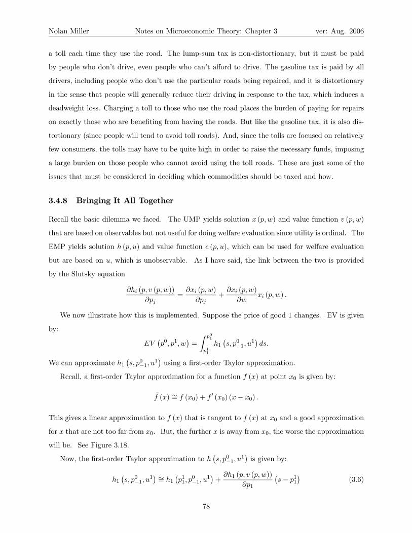
Nolan Miller Notes on Microeconomic Theory: Chapter 3 ver: Aug. 2006
a toll each time they use the road. The lump-sum tax is non-distortionary, but it must be paid
by people who don’t drive, even people who can’t afford to drive. The gasoline tax is paid by all
drivers, including people who don’t use the particular roads being repaired, and it is distortionary
in the sense that people will generally reduce their driving in response to the tax, which induces a
deadweight loss. Charging a toll to those who use the road places the burden of paying for repairs
on exactly those who are benefiting from having the roads. But like the gasoline tax, it is also dis-
tortionary (since people will tend to avoid toll roads). And, since the tolls are focused on relatively
few consumers, the tolls may have to be quite high in order to raise the necessary funds, imposing
a large burden on those people who cannot avoid using the toll roads. These are just some of the
issues that must be considered in deciding which commodities should be taxed and how.
3.4.8 Bringing It All Together
Recall the basic dilemma we faced. The UMP yields solution x (p,w) and value function v (p,w)
that are based on observables but not useful for doing welfare evaluation since utility is ordinal. The
EMP yields solution h (p, u) and value function e (p, u), which can be used for welfare evaluation
but are based on u, which is unobservable. As I have said, the link between the two is provided
by the Slutsky equation
∂hi (p, v (p,w))
∂pj=
∂xi (p,w)
∂pj+
∂xi (p,w)
∂wxi (p,w) .
We now illustrate how this is implemented. Suppose the price of good 1 changes. EV is given
by:
EV¡p0, p1, w
¢=
Z p01
p11
h1¡s, p0−1, u
1¢ds.
We can approximate h1¡s, p0−1, u
1¢using a first-order Taylor approximation.
Recall, a first-order Taylor approximation for a function f (x) at point x0 is given by:
f (x) ∼= f (x0) + f 0 (x0) (x− x0) .
This gives a linear approximation to f (x) that is tangent to f (x) at x0 and a good approximation
for x that are not too far from x0. But, the further x is away from x0, the worse the approximation
will be. See Figure 3.18.
Now, the first-order Taylor approximation to h¡s, p0−1, u
1¢is given by:
h1¡s, p0−1, u
1¢ ∼= h1
¡p11, p
0−1, u
1¢+
∂h1 (p, v (p,w))
∂p1
¡s− p11
¢(3.6)
78
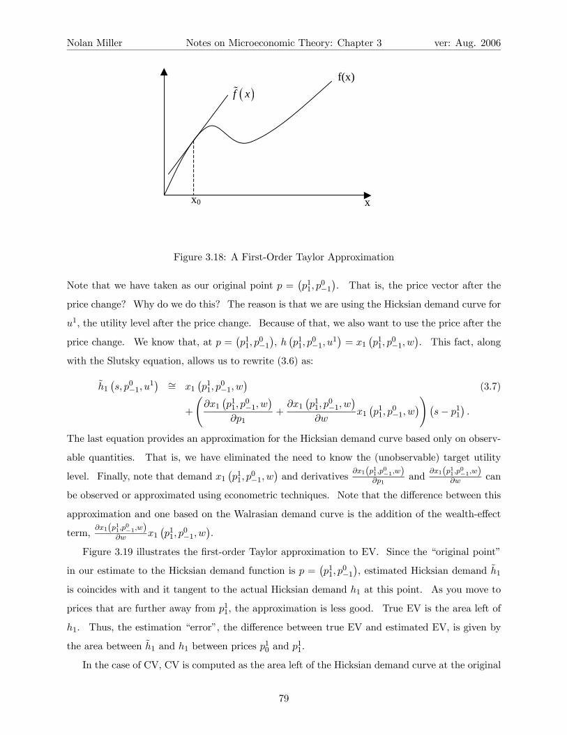
Nolan Miller Notes on Microeconomic Theory: Chapter 3 ver: Aug. 2006
x0 x
f(x)
( )f x
Figure 3.18: A First-Order Taylor Approximation
Note that we have taken as our original point p =¡p11, p
0−1¢. That is, the price vector after the
price change? Why do we do this? The reason is that we are using the Hicksian demand curve for
u1, the utility level after the price change. Because of that, we also want to use the price after the
price change. We know that, at p =¡p11, p
0−1¢, h¡p11, p
0−1, u
1¢= x1
¡p11, p
0−1, w
¢. This fact, along
with the Slutsky equation, allows us to rewrite (3.6) as:
h1¡s, p0−1, u
1¢ ∼= x1
¡p11, p
0−1, w
¢(3.7)
+
̶x1
¡p11, p
0−1, w
¢∂p1
+∂x1
¡p11, p
0−1, w
¢∂w
x1¡p11, p
0−1, w
¢!¡s− p11
¢.
The last equation provides an approximation for the Hicksian demand curve based only on observ-
able quantities. That is, we have eliminated the need to know the (unobservable) target utility
level. Finally, note that demand x1¡p11, p
0−1, w
¢and derivatives
∂x1(p11,p0−1,w)∂p1
and∂x1(p11,p0−1,w)
∂w can
be observed or approximated using econometric techniques. Note that the difference between this
approximation and one based on the Walrasian demand curve is the addition of the wealth-effect
term,∂x1(p11,p0−1,w)
∂w x1¡p11, p
0−1, w
¢.
Figure 3.19 illustrates the first-order Taylor approximation to EV. Since the “original point”
in our estimate to the Hicksian demand function is p =¡p11, p
0−1¢, estimated Hicksian demand h1
is coincides with and it tangent to the actual Hicksian demand h1 at this point. As you move to
prices that are further away from p11, the approximation is less good. True EV is the area left of
h1. Thus, the estimation “error”, the difference between true EV and estimated EV, is given by
the area between h1 and h1 between prices p10 and p11.
In the case of CV, CV is computed as the area left of the Hicksian demand curve at the original
79

Nolan Miller Notes on Microeconomic Theory: Chapter 3 ver: Aug. 2006
x1(p1,p-1,w)
p11
p10
h1(p1,p-1,u1)
( )11 1, ,h p p u−
EV
Estimation “error”
p1
x1
Figure 3.19: The First-Order Taylor Approximation to EV
80
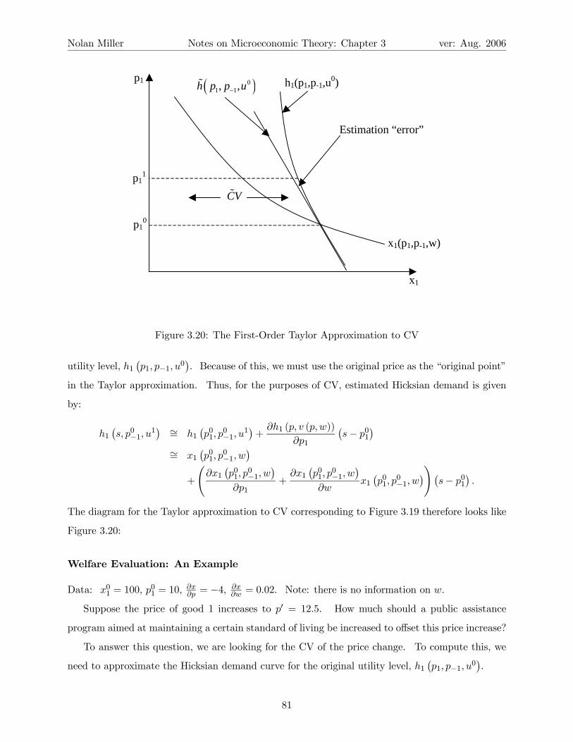
Nolan Miller Notes on Microeconomic Theory: Chapter 3 ver: Aug. 2006
x1(p1,p-1,w)
p11
p10
h1(p1,p-1,u0) ( )01 1, ,h p p u−
CV
Estimation “error”
p1
x1
Figure 3.20: The First-Order Taylor Approximation to CV
utility level, h1¡p1, p−1, u0
¢. Because of this, we must use the original price as the “original point”
in the Taylor approximation. Thus, for the purposes of CV, estimated Hicksian demand is given
by:
h1¡s, p0−1, u
1¢ ∼= h1
¡p01, p
0−1, u
1¢+
∂h1 (p, v (p,w))
∂p1
¡s− p01
¢∼= x1
¡p01, p
0−1, w
¢+
̶x1
¡p01, p
0−1, w
¢∂p1
+∂x1
¡p01, p
0−1, w
¢∂w
x1¡p01, p
0−1, w
¢!¡s− p01
¢.
The diagram for the Taylor approximation to CV corresponding to Figure 3.19 therefore looks like
Figure 3.20:
Welfare Evaluation: An Example
Data: x01 = 100, p01 = 10,
∂x∂p = −4,
∂x∂w = 0.02. Note: there is no information on w.
Suppose the price of good 1 increases to p0 = 12.5. How much should a public assistance
program aimed at maintaining a certain standard of living be increased to offset this price increase?
To answer this question, we are looking for the CV of the price change. To compute this, we
need to approximate the Hicksian demand curve for the original utility level, h1¡p1, p−1, u0
¢.
81
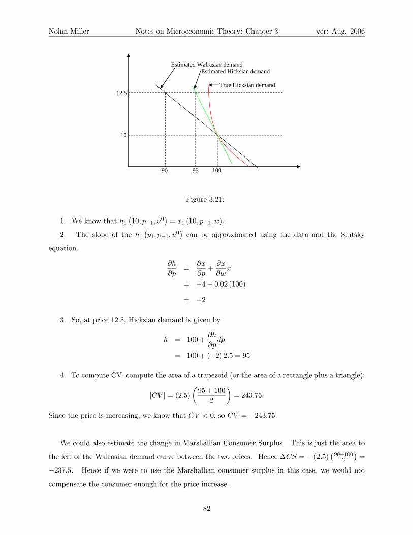
Nolan Miller Notes on Microeconomic Theory: Chapter 3 ver: Aug. 2006
12.5
10
100 95 90
Estimated Walrasian demand Estimated Hicksian demand
True Hicksian demand
Figure 3.21:
1. We know that h1¡10, p−1, u0
¢= x1 (10, p−1, w).
2. The slope of the h1¡p1, p−1, u0
¢can be approximated using the data and the Slutsky
equation.
∂h
∂p=
∂x
∂p+
∂x
∂wx
= −4 + 0.02 (100)
= −2
3. So, at price 12.5, Hicksian demand is given by
h = 100 +∂h
∂pdp
= 100 + (−2) 2.5 = 95
4. To compute CV, compute the area of a trapezoid (or the area of a rectangle plus a triangle):
|CV | = (2.5)µ95 + 100
2
¶= 243.75.
Since the price is increasing, we know that CV < 0, so CV = −243.75.
We could also estimate the change in Marshallian Consumer Surplus. This is just the area to
the left of the Walrasian demand curve between the two prices. Hence ∆CS = − (2.5)¡90+1002
¢=
−237.5. Hence if we were to use the Marshallian consumer surplus in this case, we would not
compensate the consumer enough for the price increase.
82
Nolan Miller Notes on Microeconomic Theory: Chapter 3 ver: Aug. 2006
Another thing we could do is figure that the harm done to the consumer is just the change in
price times the original consumption of this good, i.e., 2.5 (100) = 250. However, if we gave the
consumer 250 additional dollars, we would be overcompensating for the price increase.
3.4.9 Welfare Evaluation for an Arbitrary Price Change
The basic analysis of welfare change using CV and EV considers the case of a single price change.
However, what should we do if the policy change is not a single price change? For changes in
multiple prices, we can just compute the CV for each of the changes (i.e., changing prices one by
one and adding the CV (or EV) from each of the changes along a “path” from the original price to
the new price). If price and wealth change, we can add the change in wealth to the CV (or EV)
from the price changes (see below). But, what if the policy change involves something other than
prices and wealth, such a change in environmental quality, roads, etc. How do we value such a
change?
The answer is that, if we have good estimates of Walrasian demand, we can always represent
the change as a change in a budget set. After doing so, we can compute the CV is the usual way.
Part 1: Any arbitrary policy change can be thought of as a simultaneous change in
p and w.
To illustrate, suppose that we have a good estimate of consumers’ demand functions (i.e., we
fit a flexible functional form for demand using high-quality data). Let x (p,w) denote demand.
Suppose that initially prices and wealth are¡p0, w0
¢and the consumer chooses bundle x
¡p0, w0
¢.
Now, suppose that “something happens” that leads the consumer to choose bundle x0 instead of
x0. What is the CV (or EV) of this change?
The first step is to note that, if demand is quasiconcave, there is some price-wealth vector for
which x0 and x0 are optimal choices. You can find these price-wealth vectors, which we’ll call¡p0, w0
¢and (p0, w0), by solving the equations x0 =
¡p0, w0
¢and x0 = x (p0, w0). (In reality you
probably already know¡p0, w0
¢and have an observation of x0 or estimate of.) Remember, we have
a good estimate of x (p,w). Once we find (p0, w0), then we know that the change in the consumer’s
utility in going from x0 to x0is just v (p0, w0)− v
¡p0, w0
¢, and so the impact of the policy change
reduces to computing the EV or CV for this simultaneous change in p and w. Let v (p0, w0) = u0
and v¡p0, w0
¢= u0.
Part 2: Compute the EV or CV for a simultaneous change in p and w.
So, we’ve recast the policy change as a change from¡p0, w0
¢to (p0, w0), letting u0 and u0 denote
83
Nolan Miller Notes on Microeconomic Theory: Chapter 3 ver: Aug. 2006
the utility levels before and after the change. To compute EV , return to the definition of EV we
used before.
EV = e¡p0, u0
¢− e
¡p0, u0
¢Adding and subtracting e (p0, u0), we get:
EV =£e¡p0, u0
¢− e
¡p0, u0
¢¤+£e¡p0, u0
¢− e
¡p0, u0
¢¤.
But, note that e (p0, u0) = w0 and e¡p0, u0
¢= w0, so
EV =£e¡p0, u0
¢− e
¡p0, u0
¢¤+ w0 −w0, (*)
and note that£e¡p0, u0
¢− e (p0, u0)
¤is as in the definition of EV when only a price changes. So, if
only the price of good 1 changes, EV can be written as:
EV =
Z p01
p01
h1¡s, p−1, u
0¢ ds+ ¡w0 − w0¢,
and this can be estimated in the usual way from the estimated Walrasian demand curve.
If multiple prices change, we change them one by one and add up the integral from each change,
and then we add the change in wealth. That is, if prices change from¡p01, p
02, ..., p
0L
¢to (p01, p
02, ..., p
0L)
and wealth changes from w0 to w0, the EV is:
EV =
Z p01
p01
h1¡s, p02, ..., p
0L
¢ds+
Z p02
p02
h2¡p01, s, p
03, ..., p
0L
¢ds+...+
Z p0L
p0L
h2¡p01, p
02, ..., p
0L−1, s
¢ds+w0−w0.
If you replace each Hicksian demand with an estimate based on Marshallian demand and the Slutsky
equation, you can estimate this using only observables. It is tedious, but certainly possible.
This is a diagram that illustrates the whole thing. Suppose a policy change moves the con-
sumer’s consumption bundle from x0 to x0. To compute the EV, the first thing you do is find the
(p,w) for which x0 = x¡p0, w0
¢. This budget set is labeled B
¡p0, w0
¢. Then, you find the (p,w)
for which x0 is optimal, which we call (p0, w0). This budget set (red) is labeled B (p0, w0). Denote
the initial utility level u0 and the final utility level u0, and note that neither the utility levels nor
the indifference curves (which are drawn in as dotted lines for illustration) are observed.
Next, we decompose the change from¡p0, w0
¢to (p0, w0) into two parts. Part 1 is a change in
wealth holding prices fixed at p0. Let y denote the point the consumer chooses at¡p0, w0
¢, and
let uy denote the utiltiy earned. This point and the associated budget set are in blue. Note that
moving from budget set B¡p0, w0
¢to budget set B
¡p0, w0
¢is just like losing w0−w0 dollars (since
prices don’t change this is, in fact, exactly what happens). This is where the¡w0 −w0
¢term comes
84

Nolan Miller Notes on Microeconomic Theory: Chapter 3 ver: Aug. 2006
from in expression (*) above. Distance w0−w0 is denoted on the left. (Note that in the diagram,
these distances are scaled by p2, since we are showing them on the x2-axis.)
Part 2 of the decomposition is the change in prices from p0 to p0 when wealth is w0. But, note
that this just the kind of EV we computed in the simple case. That is, prices change but wealth
remains constant. Let z denote the point that offers the same utility as x0 but is chosen at prices
p0. That is, z = x¡p0, w0 +EV
¡p0, p0.w0
¢¢. The budget line supporting z is denoted in green, and
the EV for the price change from p0 to p0 at wealth w0 is just the distance that the budget shifts up
from blue B¡p0, w0
¢to green B
¡p0, w0 +EV
¡p0, p0.w0
¢¢denoted EV
¡p0, p0, w0
¢on the left. Since
EV¡p0, p0, w0
¢= e
¡p0, u0
¢− e
¡p0, uy
¢= e
¡p0, u0
¢−w0
= e¡p0, u0
¢− e
¡p0, u0
¢,
this is just like the EV’s we computed when only prices changed. This is where the£e¡p0, u0
¢− e (p0, u0)
¤comes from in expression (*) above.
The total EV is the sum of these two parts. The distance is denoted Total EV in the diagram.
Note that since the consumer ends up worse off overall, the total EV should be negative.
You could also do something similar for CV.
CV = e¡p0, u0
¢− e
¡p0, u0
¢=
£e¡p0, u0
¢− e
¡p0, u0
¢¤+he¡p0, u0
¢− e
³p0, u0´i
= w0 − w0 +he¡p0, u0
¢− e
³p0, u0´i,
and note that once again£e¡p0, u0
¢− e
¡p0, u0
¢¤is as in our original definition of CV . So, this
term can be rewritten in terms of integrals of Hicksian demand curves at utility level u0.
85

Nolan Miller Notes on Microeconomic Theory: Chapter 3 ver: Aug. 2006
x2
x0
x'
y
z
B(p0,w0)
B(p',w')
B(p0,w')
B(p',w'+EV(p0,p',w'))
w'-w0
EV(p0,p',w')
Total EV
u0
u'
uy
Figure 3.22:
86