The Torelli Group and Representations of Mapping Class Groups
119
The Torelli Group and Representations of Mapping Class Groups Tara Elise Brendle Submitted in partial fulfillment of the requirements for the degree of Doctor of Philosophy in the Graduate Schools of Arts and Sciences COLUMBIA UNIVERSITY 2002
Transcript of The Torelli Group and Representations of Mapping Class Groups

The Torelli Group and Representations
of Mapping Class Groups
Tara Elise Brendle
Submitted in partial fulfillment of the
requirements for the degree
of Doctor of Philosophy
in the Graduate Schools of Arts and Sciences
COLUMBIA UNIVERSITY
2002

c© 2002
Tara E. Brendle
All Rights Reserved

ABSTRACT
The Torelli Group and Representations
of Mapping Class Groups
Tara E. Brendle
LetMg,b,n denote the mapping class group of an orientable surface of genus
g with b boundary components and n fixed points. We prove that certain
obstructions to the existence of a faithful linear representation do not exist in
Mg,b,n for any g, b, and n. We also make explicit the relationship of three known
representations ofMg,1,0 to each other. In particular, we show how each records
the action of mapping class groups on homology and on the winding number
of curves on the surface. The action on homology is given by the well known
symplectic representation of the mapping class group ρ : Mg,b,n → Sp(2g,Z).
The kernel of ρ, denoted Ig,b,n, is known as the Torelli group. We generalize a
construction of Dennis Johnson to find relations amongst Johnson’s finite set
of generators of Ig,1,0 and Ig,0,0 and give an alternate technique which yields
commutativity relations in these Torelli groups.

Contents
1 Introduction 1
2 On the Linearity Problem for Mapping Class Groups 7
2.1 Introduction . . . . . . . . . . . . . . . . . . . . . . . . . . . . . . . . 7
2.2 The Method of Formanek and Procesi . . . . . . . . . . . . . . . . . . 10
2.3 The Connection with Mapping Class Groups . . . . . . . . . . . . . . 12
2.4 Poison Subgroups Cannot Be Embedded inMg,0,1 . . . . . . . . . . . 17
2.5 FP-Groups Do Not Embed in Mapping Class Groups . . . . . . . . . 25
3 Winding Number and Representations of Mapping Class Groups 40
3.1 Group Cohomology Background . . . . . . . . . . . . . . . . . . . . . 41
3.2 Morita’s Representation ρ3 . . . . . . . . . . . . . . . . . . . . . . . . 43
3.3 Crossed Homomorphisms Mg,1 → H . . . . . . . . . . . . . . . . . . 47
3.4 Trapp’s Representation . . . . . . . . . . . . . . . . . . . . . . . . . . 51
3.5 Perron’s Representation . . . . . . . . . . . . . . . . . . . . . . . . . 53
4 Relations in the Torelli Group 65
4.1 Johnson’s finite generating set . . . . . . . . . . . . . . . . . . . . . . 66
4.2 Lantern relations in the Torelli group . . . . . . . . . . . . . . . . . . 70
4.2.1 Johnson’s B-relations . . . . . . . . . . . . . . . . . . . . . . . 71
4.2.2 Generalized B-relations . . . . . . . . . . . . . . . . . . . . . . 75
4.2.3 Commutator relations . . . . . . . . . . . . . . . . . . . . . . 82
4.3 Symmetry of straight chain maps and further questions . . . . . . . . 90
i
A Johnson’s generators in genus 3 93
B Some calculations of relations in low genus 100
ii

Acknowledgements
I would first like to thank my advisor, Joan Birman, for all her help and advice to
me over the years. I am also grateful to Walter Neumann and Brian Mangum for
numerous helpful discussions. I thank all three, as well as Gabriel Rosenberg and
John Morgan for agreeing to be on my thesis defense committee.
I am also deeply indebted to Hessam Hamidi-Tehrani, with whom it was my great
privilege to collaborate.
I would also like to thank Oliver Dasbach for his unwavering support. In addition,
I thank many of my fellow graduate students from whom I learned a great deal, in
particular, Abhijit Champanerkar and Nathan Broaddus. Thanks also to Joe Hundley
and Omer Offen for moral support especially during job application season.
I must include a special thanks to Fran, Dolores, Laurent, Mary, and Ellie, for
their generous assistance and support during my time at Columbia. As well, thanks
to Dwight for always providing some cheer in the office.
My heartfelt thanks goes out to my parents, my sister, and Shani for always be-
lieving in me. Thanks to all the great friends I have made in New York, in particular,
to Danielle, Amy, Kathy, Meera, and especially Nancy, who, quite literally, was beside
me every step of the way.
I am also deeply grateful to and inspired by the wonderful women of the EDGE
program. I would particularly like to thank Sylvia, Rhonda, Ami, Ulrica, Diana,
Cathy, and our 37 talented participants. To that last group: if I can do this, so can
you!
And to quote the man himself: last but not least, thanks to Brendan whose
support has been simply wonderful.
iii

To my sister Suzanne
iv

1
1 Introduction
The goal of this thesis is to study certain representations and subgroups of mapping
class groups of surfaces. Our investigation has three components. First, we consider
the question of whether mapping class groups admit faithful linear representations.
We then describe connections between three known representations of certain map-
ping class groups. Finally, we construct relations among a certain generating set of
the Torelli subgroup of the mapping class group.
Let Sg,b,n denote an orientable surface of genus g with b boundary components and
n punctures. The mapping class group of Sg,b,n, denotedMg,b,n, is defined as the group
of all isotopy classes of orientation-preserving homeomorphisms of Sg,b,n to itself. In
Section 2, which consists of work conducted jointly with Hessam Hamidi-Tehrani, we
investigate a natural question which arises in the study of representations of mapping
class groups, namely, whether Mg,b,n is linear, i.e., admits a faithful representation
into GLn(K) for some field K. Mapping class groups are closely related to lattices,
which are of course linear, and also to braid groups, which were recently shown to
be linear [2],[30]. Much work has been done to try to generalize the methods used
to demonstrate linearity of braid groups to mapping class groups, but with very
limited success. On the other hand, mapping class groups are also closely related
to automorphism groups of free groups of rank n, denoted Aut(Fn). Formanek and
Procesi have demonstrated that Aut(Fn) is not linear if n ≥ 3 [14]. Hence Hamidi-
Tehrani and I took the opposite approach to the linearity question for mapping class
groups. Formanek and Procesi’s technique is to construct nonlinear groups of a
special form, which we call FP-groups. They build these groups out of two elements
of Aut(Fn) which act in a particular way on three elements of Fn. We call the group

2
generated by two such maps a poison group. Hamidi-Tehrani and I hoped to find
analogous poison subgroups in Mg,0,1, which acts naturally on π1(Sg,0,1) and then
to mimic Formanek and Procesi’s construction of FP-groups in Mg,0,1. We instead
prove the following surprising result [7].
Theorem No poison subgroups embed in Mg,0,1.
We further prove a much more general result.
Theorem No FP-groups of any kind embed in Mg,b,n for any g, b, n.
In other words, not only does the particular construction of Formanek and Procesi
fail in the case of mapping class groups, but a more general obstruction to linearity
does not exist in any mapping class groups. This gives very strong evidence that
mapping class groups may in fact be linear.
We next turn our attention to known representations of mapping class groups.
In Section 3, we describe three representations of mapping class groups which arise
in very different contexts yet each carry much of the same geometric information.
Section 3 is largely expository, and seeks to fill what seems to be a gap in the literature
by clarifying some connections between the three representations.
The group Mg,b,n acts naturally on H = H1(Sg,b,n), giving rise to what is known
as the symplectic representation of the mapping class group.
ρ :Mg,b,n → Sp(2g,Z).
The kernel of this representation is known as the Torelli group, denoted Ig,b,n. In
[39], Morita constructs representations of Mg,1,0 using an extension of Johnson’s
“torsion” homomorphism τ : Ig,1,0 → Λ3H described in [20]. The map τ enables us

3
to determine the action of mapping class groups on the winding number of curves
on a surface relative to some non-vanishing vector field. Morita’s representation also
contains all the information of the symplectic representation ρ.
Trapp [46] (and independently Sipe [44]) gives a linear form of Morita’s repre-
sentation interpreted explicitly in terms of the action of Mg,1,0 on winding numbers
and on homology. Perron also linearizes Morita’s representation, instead building a
representation ψ : Mg,1,0 → GL4g(Z[d1, . . . , d2g]) by extending a representation of
a certain Artin group [41]. We present a method for extracting the same winding
number and homology information directly from Perron’s representation.
The Torelli group plays a prominent role in the study of representations of mapping
class groups. Hence we focus on this fascinating and poorly understood subgroup of
Mg,b,n.
Surprisingly little is known about the structure of the Torelli group, but the first
serious progress in this direction was made by Dennis Johnson, who wrote a wonderful
series of papers on the Torelli group ([20], [21], [22], [24], [25], and [26], all summarized
nicely in [23]). One of Johnson’s most important results is that both Ig,1,0 and Ig,0,0
are finitely generated for g ≥ 3 [22]. (Mess later showed that I2,b,n is infinitely
generated [36].) Johnson also discovered an important surjective map τ : Ig,1,0 →
Λ3H, giving the first nice abelian quotient of the Torelli group.
One important question which remains open, however, is the question of whether
the Torelli group admits a finite presentation. It is known that Mg,b,n is finitely
presentable (see [16], also [48], [49], [31]). As one approach to this question, we ask
what relations can be found amongst Johnson’s generators, which remain the only
known finite set of generators of the Torelli group. This is no easy task; the order

4
of Johnson’s generating set for the Torelli group is exponential in the genus g. As a
starting point, we have a technique developed by Johnson which he used to find two
families of relations amongst various elements of the Torelli group, including some
which are not in his generating set. Johnson uses so-called “lantern relations” in the
full mapping class group to obtain these relations in the Torelli group.
We first show how to generalize one of Johnson’s families of generators so as to
relate only elements from his generating set in a way that yields on the order of g3
relations for genus g ≥ 4, using his same technique. The relation is as follows.
Generalized B-Relation In Ig,1,0, for g ≥ 4 and for 2 ≤ l < k ≤ g − 1, we have
[W−1k ∗ (PgP
−1l )][W−1
2 ∗ Pk] = [W−1g ∗ (PkP
−1l )][W−1
2 ∗ Pg].
In the above relation, the Wi are a certain type of Johnson generator and the Pj are
products of two Johnson generators, which also happen to be commutators in the full
mapping class group. We obtain from the construction of the relation the following
corollary, which Johnson has already proved for genus 3 [22]).
Corollary 1.1 There are g − 2 extraneous generators of Ig,1,0 in Johnson’s set.
We then give an alternate construction, which also arises from lantern relations
but avoids some of the difficulties of Johnson’s original technique. This second method
yields a new kind of relation, in fact, a commutativity relation.
General Commutator Relation In Ig,1,0, for g ≥ 4, we have the following rela-
tion:
[(B−11 A1B3), (A2B
−12 )] = 1.

5
Each curve Ai or Bj is a type of Johnson generator which will be described in
detail in Section 4. Taken together, the Ai and Bj satisfy a certain intersection
pattern. There are on the order of g5 of these commutativity relations for g ≥ 4.
We remark that each relation given here, both B-relations and commutator relations,
actually represent many more conjugate relations. For example, the simplest case
of the generalized B-relation actually yields 33 distinct relations amongst Johnson
generators (see Appendix B).
We will also briefly discuss a certain symmetry satisfied by the vast majority of
the pairs of Dehn twist curves appearing in the Johnson generating set and some
potential applications to the linearity question for the Torelli group. We then present
a list of questions, including many raised by this investigation, intended to outline a
plan for future study of the Torelli group.
It is worth elaborating at this point on the earlier claim regarding the importance
of the role played by the Torelli group in the study of representations of Mg,b,n. It
comes as no surprise that the Torelli group plays a key role in any representation con-
taining symplectic information. For example, the map τ (to be precise, the contraction
of τ) turns out to be important in the Trapp, Morita, and Perron representations of
the full mapping class group, as discussed in Section 3.
More surprising is the fact that the Torelli group appears in the study of other rep-
resentations which arise in ostensibly very different contexts. For example, Kasahara
recently showed that Johnson’s homomorphism factors through the Jones representa-
tion ofM2 restricted to I2 [27]. In addition, the representations ofMg arising from
topological quantum field theories (TQFTs) also connect with Johnson’s work in an

6
interesting way. The TQFT representations of Reshetikhin-Turaev are indexed by a
integer parameter r. Wright has calculated these representations explicitly for r = 4
and found that the restriction of the representation in this case to Ig is precisely the
sum of the Birman-Craggs homomorphisms from Ig to Z/2Z [51]. Johnson shows
in [21] that the sum of the Birman-Craggs homomorphisms is related to his map τ ,
though neither factors through the other, giving a possibly interesting connection to
the representations discussed above.

7
2 On the Linearity Problem for Mapping Class
Groups
In this section we seek to provide some insight into the question of whether mapping
class groups are linear. Mapping class groups are often compared with both arithmetic
and automorphism groups, and in many ways the three groups are similar and support
analogous theories. (There is a nice discussion of this by Karen Vogtmann in [47].
Another good survey of this subject was recently given by Martin Bridson in a series
of lectures at Columbia University.) The property of linearity, however, is an area in
which these groups differ. Lattices, of course, are linear, but Formanek and Procesi
showed in [14] that Aut(Fn) is not linear for n ≥ 3 (it follows that Out(Fn) is also
not linear for n ≥ 4), leading one to ask on which side mapping class groups should
fall.
The work in this section was conducted jointly with Hessam Hamidi-Tehrani. We
present it here as it appeared in [7], with reference numbers of sections and theorems
appropriately altered.
2.1 Introduction
The question of whether mapping class groups are linear has been around for some
time. The recent work of Bigelow [2] and also Krammer [30] in determining that the
braid group is linear has renewed interest in the subject, due to the close relationship
between mapping class groups and braid groups. Let Sg,b,n denote a surface of genus g
with b boundary components and n fixed points. LetMg,b,n denote the mapping class

8
group of Sg,b,n. We assume throughout that maps fix boundary components pointwise.
Bigelow and Budney [3] and independently Korkmaz [29] recently determined that
M2,0,0 is linear. Korkmaz also showed in [29] that mapping class groups contain very
large linear subgroups, namely, the hyperelliptic subgroups. However, the question
of linearity remains open for mapping class groups of surfaces of genus 3 or greater.
Let Fn denote the free group of rank n. It is well known that Out(F2) and Aut(F2)
are linear. The former fact is due to Nielsen [40], and the latter follows by [12] from
the linearity of the 4-string braid group B4, which is due to Krammer [30].
On the other hand, Formanek and Procesi demonstrated in [14] that Aut(Fn) is
not a linear group for n ≥ 3. A simple corollary of this result is that Out(Fn) is not
linear for n ≥ 4. The well-known fact due to Nielsen [33] thatMg,0,0 is isomorphic to
Out(π1(Sg,0,0)) suggests that it may be possible to apply the methods of Formanek
and Procesi to mapping class groups, though it may not be immediately clear how to
do so.
Formanek and Procesi define a class of nonlinear groups, which we will generalize
slightly and refer to as Formanek and Procesi groups, or FP-groups for short. We will
show that the existence of FP-subgroups ofMg,0,1 would imply that Mg+k,0,0 is not
linear for k ≥ 1. We will also focus our attention on a special kind of automorphism
group, which we call a poison group. We will describe the particular method of
Formanek and Procesi for constructing FP-groups from poison subgroups.
This work originated in an attempt to use the methods of Formanek and Procesi
to show that Mg,0,0 is not linear for g ≥ 3. We prove instead that the essential
building blocks of the Formanek and Procesi method do not exist in mapping class
groups, first in a special case.

9
Theorem A Poison subgroups cannot be embedded in Mg,0,1.
Thus the particular technique of Formanek and Procesi fails to show that certain
mapping class groups are not linear. We then generalize this result as follows.
Theorem B FP-groups do not embed in Mg,b,n for any g, b, and n.
Our paper is organized as follows. In Section 2.2, we give an overview of the
methods of Formanek and Procesi for constructing a nonlinear subgroup of Aut(Fn)
from a poison subgroup. In Section 2.3, we establish connections between certain
mapping class groups and the automorphism group of a closed surface. In Section
2.4 we prove Theorem A. In Section 2.5 we prove Theorem B using very different
techniques from those used in Section 2.4. Though Theorem A is a special case of
Theorem B, we include a separate proof of Theorem A both for the sake of highlighting
the particular construction of Formanek and Procesi and also because the methods
used are interesting in their own right. The reader should note, however, that Sections
2.3, 2.4, and 2.5 are completely independent of one another. For example, the reader
interested only in Theorem B could read Sections 2.1, 2.2, and 2.5 without any loss
of continuity.
Acknowledgements The authors would like to express their sincere gratitude to
Joan Birman and Alex Lubotzky for suggesting the search for poison subgroups in
mapping class groups, and also to Matthew Zinno for helping to point us in the
other direction. We thank all three, as well as Walter Neumann, Brian Mangum,

10
Gabriel Rosenberg, and Abhijit Champanerkar for many useful discussions. We are
also grateful to the referee for many helpful questions and suggestions.
The first author was partially supported under NSF Grant DMS-9973232. The
second author was partially supported by PSC-CUNY Research Grant 63463 00 32.
2.2 The Method of Formanek and Procesi
Let G be any group, and let H(G) denote the following HNN-extension of G×G:
H(G) = 〈G×G, t | t(g, g)t−1 = (1, g), g ∈ G〉.
In other words, conjugation by t in the HNN-extension carries the diagonal subgroup
G × G onto its second factor. Formanek and Procesi show in the following theorem
that such groups exhibit special behavior under a linear representation.
Theorem 2.1 (Formanek and Procesi, [14]) Let G be a group. Then the image
of the subgroup G × {1} under any linear representation of H(G) is nilpotent-by-
abelian-by-finite.
Corollary 2.2 Let G be a group, and K a normal subgroup of H(G) such that the
image of G× {1} in H(G)/K is not nilpotent-by-abelian-by-finite. Then H(G)/K is
not linear.
Proof. Let ρ : H(G)/K → GLN(k) be a linear representation where k is a field.
Let π : H(G) → H(G)/K be the natural projection map. Then ρ ◦ π is a linear
representation of H(G) and hence by Theorem 2.1, ρ(π(G × {1})) is nilpotent-by-
abelian-by-finite. Thus ρ is not faithful.

11
We will call a group of the type described in Corollary 2.2 a Formanek and Pro-
cesi group, or FP-group for short. We now describe the particular construction of
Formanek and Procesi in demonstrating the nonlinearity of Aut(Fn) for n ≥ 3.
Let G be any group. Let x1, x2, x3 be elements of G such that 〈x1, x2, x3〉 ∼= F3.
Let φ1, φ2 ∈ Aut(G) be two maps such that
1. φi(xj) = xj, i, j = 1, 2, and
2. φi(x3) = x3xi, i = 1, 2.
We will call the subgroup 〈φ1, φ2〉 a poison subgroup of Aut(G). We can define poi-
son subgroups of the mapping class group Mg,0,1 analogously, since in this case the
mapping class group acts on π1(Sg,0,1). Notice that the second condition implies that
〈φ1, φ2〉 ∼= F2. Thus poison groups, being isomorphic to the linear group F2, are
not themselves a kind of FP-group. However, as the following lemma shows, their
existence in an automorphism group Aut(G) implies that Aut(G) is not linear (hence
the name “poison groups”, though it suggests a bias towards linearity).
Lemma 2.3 Let G be any group. If Aut(G) contains a poison subgroup, then it
contains an FP-subgroup isomorphic to H(F2).
Proof. Let 〈φ1, φ2〉 be a poison subgroup in Aut(G). Following Formanek and Pro-
cesi’s argument in [14], let αi ∈ Aut(G) denote conjugation by xi. Consider the
group
H = 〈φ1, φ2, α1, α2, α3〉.
First, note that 〈α1, α2, α3〉 is a normal subgroup of H since both φ1 and φ2 preserve
the subgroup 〈x1, x2, x3〉. Now let w(a, b) denote any non-trivial reduced word in

12
the free group on the letters a and b. By definition of a poison subgroup, we know
that w(φ1, φ2)(xi) = xi for i = 1,2. This tells us that if w(φ1, φ2) is in 〈α1, α2, α3〉,
then w(φ1, φ2) must induce conjugation by an element in 〈x1, x2, x3〉 ∼= F3, which
commutes with x1 and x2. But the only such element is the identity. Hence w(φ1, φ2)
must be the identity map. But we know this is not the case since
w(φ1, φ2)(x3) = x3w(x1, x2). (1)
This tells us that the images of φ1 and φ2 mod 〈α1, α2, α3〉 will generate a free group.
Clearly, the images of φ1 and φ2 also generate the quotient of H by 〈α1, α2, α3〉 , and
so we have a split exact sequence
1→ 〈α1, α2, α3〉 → H → 〈φ1, φ2〉 → 1. (2)
Thus the only relations we have in a presentation for H are given by conjugation, as
follows:
H = 〈φ1, φ2, α1, α2, α3 | φiαjφ−1i = αj, φiα3φ
−1i = α3αi, i, j = 1, 2〉. (3)
Rewriting the second set of relations, we obtain α3(αiφi)α−13 = φi, i = 1, 2. Since
〈φ1, φ2〉 ∼= 〈α1, α2〉 ∼= F2, we have that H ∼= H(F2), with α3 playing the role of the
element t. Since F2 is not nilpotent-by-abelian-by-finite, H(F2) is an FP-group.
2.3 The Connection with Mapping Class Groups
Our motivation for the work in this paper is the following observation, the proof of
which we defer to the end of the section.

13
Claim 2.4 If a poison subgroup exists in Mg,0,1 for g ≥ 2, then the groups Mg+k,0,0
are not linear for k ≥ 1.
We have been abusing terminology a bit by talking about poison subgroups in
Mg,0,1 and also in the context of automorphism groups. The distinction between the
two contexts is unnecessary for our purposes, as the following lemma shows, since
these mapping class groups are isomorphic to automorphism groups.
Lemma 2.5 Mg,0,1∼= Aut(π1(Sg,0,0)), for g ≥ 2.
Proof. We begin with the exact sequence
1→ Inn(π1(Sg,0,0))→ Aut(π1(Sg,0,0))→ Out(π1(Sg,0,0))→ 1.
By the well-known theorem of Nielsen [33], we have that Out(π1(Sg,0,0)) ∼= Mg,0,0.
In addition, since π1(Sg,0,0) is centerless, we can replace Inn(π1(Sg,0,0)) with π1(Sg,0,0)
(see, for example, [8]) to obtain
1→ π1(Sg,0,0)→ Aut(π1(Sg,0,0))→Mg,0,0 → 1. (4)
By [4], we also have the following exact sequence:
1→ π1(Sg,0,0)→Mg,0,1 →Mg,0,0 → 1. (5)
Every short exact sequence 1 → N → E → G → 1 induces a homomorphism
G → Out(N), defined as follows. Let g ∈ G, and let eg be a lift of g ∈ E. Now, E
acts onN by conjugation, hence we can think of eg as an element of Aut(N). However,
since N is not necessarily abelian, this map is only well defined up to conjugation
by an element of N . Thus we get a map G → Out(N). According to Corollary 6.8

14
of [8], given any short exact sequence as above, with N centerless, there is a unique
“middle group” E corresponding to any given homomorphism G→ Out(N).
In Sequence 4 above, it is clear that the map induced is the Nielsen isomorphism
between Mg,0,0 and Out(π1(Sg,0,0)). In Sequence 5, as discussed in [4], the image
of a generator a of π1(Sg,0,0) is the so-called “spin map” associated to each curve,
which induces conjugation by that curve, but can be more easily understood as a
product of opposite Dehn twists about the boundary of an annular neighborhood of
the curve a. In other words, if α and β are the two boundary curves, then the spin
map associated to the curve a can be written as TαT−1β , where Tγ denotes the Dehn
twist about the curve γ. Let φ ∈ Mg,0,0, and let φ denote a lift of φ in Mg,0,1.
Then φTαT−1β φ−1 = Tφ(α)T
−1
φ(β), which is precisely the spin map associated to φ(a).
Thus, we are simply looking at the action of φ on π1(Sg,0,0), but since φ does not
necessarily fix the basepoint, φ is getting mapped to the class of φ in Aut, modulo
inner automorphisms. In other words, the induced map fromMg,0,0 → Out(π1(Sg,0,0))
is also the Nielsen isomorphism. Now since π1(Sg,0,0) has a trivial center, we apply
Corollary 6.8 of [8], and the lemma is proved.
Remark 2.6 The isomorphism given in Lemma 2.5 has received some attention in
the literature, though perhaps not as much as it deserves. The map itself is the
obvious one, namely, any homeomorphism of a surface with one fixed point induces a
natural automorphism of the fundamental group of the closed surface with the fixed
point taken as base point. From the geometric point of view, it is not immediately
clear that this map from Mg,0,1 to Aut(π1(Sg,0,0)) should be a surjection, i.e., it is

15
not necessarily obvious that all elements of Aut(π1(Sg,0,0)) should be topologically
induced.
Lemma 2.7 If Aut(π1(Sg,0,0)) is not linear, then Mg,1,0 is not linear.
Before proving the lemma, we make a few observations. From Chapter 4, Section
1 of [4] and Lemma 2.5 we have the short exact sequence
1→ Z→Mg,1,0 → Aut(π1(Sg,0,0))→ 1. (6)
We note that Z is actually the center of Mg,1,0, generated by a Dehn twist about
the boundary curve. Now Aut(π1(Sg,0,0)) is the quotient of Mg,1,0 by Z. In general,
the quotient of a linear group is not necessarily linear, but the extra information we
have about the kernel in this case will allow us to draw the desired conclusion. The
following two theorems are proved in [50]. Note that the term “closed” refers to the
Zariski topology.
Theorem 2.8 Let G be a linear group and H a closed normal subgroup of G. Then
G/H is also linear.
Theorem 2.9 The centralizer of any subset of a linear group is closed.
Proof of Lemma 2.7 Since Z is the center of Mg,1,0, it is normal and also closed
by the above. Thus we can apply Theorem 2.8 to the surjection given in Sequence 6,
and Lemma 2.7 follows directly.

16
We are now ready to prove the claim.
Proof of Claim 2.4 Suppose thatMg,0,1 contains a poison subgroup. Then by the
isomorphism of Lemma 2.5, Aut(π1(Sg,0,0)) also contains a poison subgroup. Then
Aut(π1(Sg,0,0)) is not linear by Lemma 2.3. Now by Lemma 2.7, Mg,1,0 is also not
linear. The claim follows from the fact thatMg,1,0 is a subgroup ofMg+k,0,0, for k ≥ 1.
Although this fact is well-known, for the sake of completeness we include a proof as
follows. Consider Sg,1,0 as a subsurface of Sg+k,0,0. Let h be the homomorphism
from Mg,1,0 to Mg+k,0,0 defined by extension to the identity on Sg+k,0,0 \ Sg,1,0. Let
f ∈ ker(h) such that f 6= id. The mapping class h(f) of Sg+k,0,0 keeps the subsurface
Sg,1,0 invariant up to isotopy. According to Section 7.5 in [19], h(f) induces a well
defined mapping class in π0(Diff(Sg,1,0)) (the group of homeomorphisms of Sg,1,0 up
to isotopy not necessarily fixing ∂Sg,1,0). But since h(f) = id and by the definition
of h, this implies that f induces the identity in π0(Diff(Sg,1,0)), which implies that f
could only be a non-trivial power of a Dehn twist in the ∂Sg,1,0. Then by definition,
h(f) will also be a non-trivial power of a Dehn twist, which is a contradiction.
Remark 2.10 We have defined poison subgroups in the context of Mg,0,1 and also
in the context of automorphism groups, but the definition also makes sense in the
context of any group action on another group. Thus one could use this as a general
approach to the linearity question for any such group.

17
2.4 Poison Subgroups Cannot Be Embedded in Mg,0,1
Our strategy for proving this result will be to decompose the surface S = Sg,0,0
into subsurfaces in a particular way. We then use the machinery of graphs of groups
(described in detail in [1]) to analyze the action of the generators of a poison subgroup
ofMg,0,1 on the elements x1, x2, x3 ∈ π1(S). After completion of the proof of Theorem
A, we discovered that similar methods involving graphs of groups and normal forms
were used by Levitt and Vogtmann in [32] to give an algorithm for the Whitehead
problem for surface groups. There is a major difference, however, in that we are not
given the curves x1, x2, and x3, and hence we cannot apply their algorithm directly,
nor would our proof be significantly shortened by direct reference to their results.
Thus we have kept the proof of Theorem A in its original form for the sake of self-
containment. We have, however, found it useful to adopt their methods for the
decomposition of the surface S.
Throughout this section assume that g ≥ 2, since Theorem A is clear when g ≤ 1.
Fix a point ∗ ∈ S, and identify Sg,0,1 with (S, ∗). We use the point ∗ as the base
point for the fundamental group of S. Let 〈φ1, φ2〉 be a poison subgroup in Mg,0,1.
Then there are elements x1, x2, x3 ∈ π1(S, ∗) such that 〈x1, x2, x3〉 ∼= F3 and
1. φi(xj) = xj i, j = 1, 2, and
2. φi(x3) = x3xi i = 1, 2.
In what follows, we will choose appropriate representatives for φi and xj (denoted
by the same names by abuse of notation) such that, among other things, a power of
φi fixes a regular neighborhood of xj pointwise. To this end our main tool will be the

18
following result of Hass and Scott [15]. For y1, y2 ∈ π1(S, ∗), let
Stab(y1, y2) = {φ ∈ Mg,0,1 | φ(yi) = yi, i = 1, 2}.
Lemma 2.11 Let y1, y2 be distinct elements of π1(S, ∗), which are not proper powers.
Then there exists a representative of yi (denoted by yi) and a subsurface A formed
by a regular neighborhood N of y1 ∪ y2 together with all disk components of S \ N ,
such that, for any φ ∈ Stab(y1, y2), φ has a representative homeomorphism φ such
that φ(A) = A.
This lemma follows from Theorem 2.1 in [15] together with the discussion in the
beginning of page 32 in the same paper. For further details see Section 2.1 in [32].
Remark 2.12 Notice that, in Lemma 2.11, if φ ∈ Stab(y1, y2), the map φ induces a
unique mapping class in π0(Diff(A, ∗)) (see Section 7.5 in [19]).
Since it is possible that x1 and x2 are proper powers, we need the following well-
known lemma, adapted from [32].
Lemma 2.13 Given a nontrivial element x ∈ π1(S, ∗) , there exists a unique y ∈
π1(S, ∗) and a unique t ≥ 1 such that y is not a proper power and x = yt.
Proof. A proof is given in [32] (Lemma 2.3). Though we will not give details, we note
that it is also possible to prove this lemma by elementary hyperbolic geometry, using
the discrete action of π1(S, ∗) on the upper half plane by hyperbolic isometries.

19
Corollary 2.14 Let z1, z2 ∈ π1(S, ∗) be such that zN1 = zN
2 for some N ≥ 1. Then
z1 = z2.
Proof. Using Lemma 2.13 let ytii = zi such that yi is not a proper power and ti ≥ 1,
for i = 1, 2. Let x = yt1N1 = yt2N
2 . By the uniqueness guaranteed by Lemma 2.13, we
have y1 = y2 and t1N = t2N . Hence z1 = z2, as desired.
Using Lemma 2.13, we can choose elements yi which are not proper powers and
ti ≥ 1 such that xi = ytii for i = 1, 2. Then we know that φi(y
tjj ) = y
tjj , which
implies that φi(yj) = yj, by Corollary 2.14. Notice that y1 and y2 are distinct since
〈x1, x2〉 ∼= F2. We choose yi and A according to Lemma 2.11. Let π0(Diff(S,A))
be the subgroup ofMg,0,1 consisting of mapping classes which have a representative
keeping A fixed pointwise. We now adapt Lemma 3.1 of [32] to our purposes, and
repeat their argument nearly verbatim.
Lemma 2.15 The subgroup π0(Diff(S,A)) has finite index in Stab(y1, y2).
Proof. First note that A is not an annulus, since x1 and x2 generate a free group.
Using Lemma 2.11 (and noting Remark 2.12), we can define a map ρ from Stab(y1, y2)
to π0(Diff(A, ∗)). Now we claim that the image of ρ is finite. To see this, let k be any
positive integer. Let Tk denote the set of homotopy classes of simple closed curves
in A whose intersection number with y1 and y2 is at most k. Then Tk is finite, since
A\ (y1 ∪ y2) is composed entirely of disks and annuli. Any map φ ∈ Stab(y1, y2) will
preserve the intersection number of a curve with y1 and y2, and hence Stab(y1, y2)
acts on the set Tk. Now choose a finite set W of simple closed curves in A whose
image completely determines an element of π0(Diff(A, ∗)). Let k be bigger than the

20
intersection number of any element in W with y1 and y2. Thus the class of φ restricted
to A in π0(Diff(A, ∗)) is completely determined by the action of φ on Tk. But the set
of permutations of Tk is finite, and hence the image of Stab(y1, y2) under ρ is finite.
Now let ι : π0(Diff(A, ∗)) → Out(π1(A, ∗)) be the natural homomorphism. The
image of ι ◦ ρ is also finite by the above argument. Now any element φ ∈ ker(ι ◦ ρ)
induces an inner automorphism on π1(A, ∗), i.e., φ(z) = czc−1. The element c has to
commute with both y1 and y2, which implies that c has to be a power of both y1 and
y2 since the centralizer of an element in a surface group is cyclic (this is an exercise
in elementary hyperbolic geometry), and y1 and y2 are not proper powers. But this
implies that c = 1 since x1 and x2 generate a free group. Hence φ induces the identity
on π1(A, ∗). Picking a set of simple generators for π1(A, ∗), one can use an isotopy
of the surface to make sure that φ keeps them fixed pointwise, by [13]. Then one can
further isotope φ to make sure φ keeps A invariant pointwise by Alexander’s lemma
[43]. Hence ker(ι ◦ ρ) is contained in π0(Diff(S,A)), which proves the lemma.
Proposition 2.16 There exists an integer M such that φMi fixes A pointwise (up to
isotopy).
Proof. We know φi ∈ Stab(y1, y2) for i = 1, 2. Hence by Lemma 2.15, there is an
integer Mi ≥ 0 such that φMi
i ∈ π0(Diff(S,A)). Letting M = LCM(M1,M2), we have
φMi ∈ π0(Diff(S,A)) for i = 1, 2.
From this point on, we assume that we are working with the particular represen-
tative of φMi which fixes A pointwise.

21
B3
b3γ3,1
γ3,2
B2
b2γ2,1
e2,1e3,1
e3,2
∗
A
γ1,1
e1,1
b1
B1
Br
br
Figure 1: The decomposition of the surface S.
ej,k γj,kcj,k
e′′j,k
e′j,k
∗
bj
Figure 2: The subarcs of ej,k.

22
Let B1, · · · ,Br be the respective closures of each component of S \ A. Each com-
ponent is Bj attached to A along one or more circles. Hence A∩Bj consists of nj ≥ 1
circles, which we denote by γj,1, · · · , γj,nj.
In what follows we will use this decomposition of S into the subsurfaces A,Bj to
construct a graph of groups G whose fundamental group will give a decomposition of
π1(S, ∗). To that end, we introduce some notation.
For an oriented arc e let start(e) and end(e) be the starting and ending points
of the arc e, respectively. Also, let e be the same arc with the opposite orientation.
In the following discussion, let the pair of indices j, k be such that 1 ≤ j ≤ r, and
1 ≤ k ≤ nj.
Choose base points bj ∈ Bj. Notice that φMi fixes each Bj setwise. Hence we
further isotope φMi so that it fixes bj, for i = 1, 2. See Figure 1.
Choose oriented arcs ej,k connecting ∗ to bj for 1 ≤ j ≤ r and 1 ≤ k ≤ nj. Choose
each arc ei,j such that it intersects γj,k exactly once, and does not intersect any other
γ’s. Moreover, we make the choices in such a way that if (j, k) 6= (j ′, k′), then ej,k
and ej′,k′ do not intersect except possibly at the endpoints. Let cj,k be the point of
intersection of ej,k with γj,k. Also, let e′j,k be the subarc of ej,k connecting ∗ to cj,k,
and let e′′j,k be the subarc from cj,k to bj. See Figure 2.
Let G be the graph embedded in S with vertices ∗, b1, · · · , br and geometric edges
ej,k as above. As a technical point, the arcs with the opposite orientation ej,k are also
considered edges of the graph G but not drawn separately.
We use the graph G to construct a graph of groups. To each vertex of G we
assign the fundamental group of the subsurface in which it is located, namely, to ∗
we assign A = π1(A, ∗), to bj we assign Bj = π1(Bj, bj). To each edge ej,k we assign

23
Γej,k= π1(γj,k, cj,k) ∼= Z. Also, let Γej,k
= Γej,k. We also have natural injections
of the edge groups into the adjoining vertex groups as follows: for any ej,k, since
start(ej,k) = ∗, the vertex group for start(ej,k) is A. We have αej,k: Γej,k
→ A defined
by αej,k(x) = e′j,kxe
′
j,k. Corresponding to end(ej,k), we have αej,k: Γej,k
→ Bj which
is defined by αej,k(x) = e′′j,kxe
′′
j,k. For the edges ej,k set αej,k= αej,k
and αej,k= αej,k
.
Let G be the graph of groups constructed by the above data. By the generalized
Van Kampen theorem, π1(S, ∗) is isomorphic to the fundamental group of the graph
of groups π1(G, ∗).
To understand the elements of π1(G, ∗), we quote some definitions from [1]. A loop
based at ∗ in G is a sequence
t = (g0, ε1, g1, · · · , εn, gn)
where εi are edges of G and (ε1, · · · , εn) is a loop in G with start(ε1) = ∗ and end(εn) =
∗. Also, g0 and gn are in A, and for 0 < i < n, each gi is in the group assigned to
end(εi) = start(εi+1). A loop t in G is reduced if either n = 0 and g0 6= 1, or n > 0 and
whenever εi+1 = εi, we have gi /∈ αεi(Γεi
). Geometrically, one can think of t as a loop
in S, with gi being loops in respective subsurfaces, and εi as arcs connecting these
loops. From this point of view, a reduced loop on S does not “travel” to a component
Bj unnecessarily.
By [1], any non-trivial element of π1(G, ∗) can be written as |t| = g0ε1g1 · · · εngn,
where t is a reduced loop as above.
Remark 2.17 The reduced loop representing 1 is the empty sequence.
Remark 2.18 A non-reduced loop can be made into a reduced loop which represents
the same element in π1(G, ∗) by the process of combing. Namely, if a loop t of length

24
n > 1 is not reduced, it has a subsequence of the form (gi−1, εi, αεi(hi), εi). One can
replace this subsequence with (gi−1αεi(hi)). This process reduces the length, so after
finitely many steps one arrives at a reduced loop.
The following theorem is proved in [1].
Theorem 2.19 Let t = (g0, ε1, g1, · · · , εn, gn) and t′ = (g′0, ε′
1, g′
1, · · · , ε′
m, g′
m) be two
reduced loops such that |t| = |t′| in π1(G). Then n = m, εi = ε′i for 1 ≤ i ≤ n, and
there exist hi ∈ Γεisuch that
1. g′0 = g0 αεi(h1)
−1,
2. g′i = αεi(hi) gi αεi+1
(hi+1)−1,
3. g′n = αεn(hn) gn.
Notice that in the above theorem the elements of the form αε(h) come from the
circles γj,k.
Proof of Theorem A. Suppose 〈φ1, φ2〉 ≤ Mg,0,1 is a poison subgroup with respect
to x1, x2, x3 ∈ π1(Sg,0,0, ∗). We construct the graph of groups G as above, with
π1(G, ∗) ∼= π1(Sg,0,0, ∗). In the following we will identify these two groups.
By Proposition 2.16, we can choose an integer M such that φMi fixes A pointwise.
Since φMi also sends each Bj to itself fixing the base points, we can see that φM
i (ej,k) =
ej,kpj,k where pj,k ∈ Bj. Similarly φMi (ej,k) = pj,k
−1ej,k.

25
We will now simplify notation a bit by letting φ stand for φM1 . Let x3 = |t| where
t is the reduced loop t = (g0, ε1, g1, · · · , ε2n, g2n). Notice that since the graph G is
“star-shaped”, the length of the loop must be even. Therefore
φ(x3) = |(g0, ε1, p1φ(g1)p2−1, ε2, g2, ε3, p3φ(g3)p4
−1, ε4, · · · , p2n−1φ(g2n−1)p2n−1, ε2n, g2n)|
(each pi is in the group which makes this a well-defined path). Now by the condition
φ1(x3) = x3x1, which implies that φ(x3) = x3xM1 , we get the equality
|(g0, ε1, p1φ(g1)p2−1, ε2, g2, ε3, p3φ(g3)p4
−1, ε4, · · · , p2n−1φ(g2n−1)p2n−1, ε2n, g2n)| =
|(g0, ε1, g1, · · · , ε2n, g2nxM1 )|.
Let t′ and t′′ be the paths appearing on the left and right hand sides of the above
equation respectively. Since the path t is reduced, so is t′′. If t′ is not reduced, by
Remark 2.18 we can comb it to a reduced path t′red. By the equality and Theorem 2.19,
t′red must have the same length as t′′, which means t′ was reduced in the first place.
Using Theorem 2.19 again, there is an h1 ∈ Γε2nsuch that g2nx
M1 = αε2n
(h1) g2n, i.e.,
xM1 = g2n
−1αε2n(h1) g2n. Similarly, using φ2 in place of φ1, there exists an h2 ∈ Γε2n
such that xM2 = g2n
−1αε2n(h2)g2n. But Γε2n
∼= Z, therefore h1, h2 commute, which
implies xM1 , x
M2 commute. This is a contradiction, since 〈x1, x2〉 ∼= F2.
2.5 FP-Groups Do Not Embed in Mapping Class Groups
We begin by showing how to narrow our search for an FP-subgroup in a mapping
class group.

26
Lemma 2.20 Suppose that Mg,b,n contains an FP-subgroup. Then it contains an
FP-subgroup H which is isomorphic to a quotient of H(F2). Moreover, the image of
F2 × {1} in H is isomorphic to F2.
Proof. Suppose Mg,b,n contains an FP-subgroup. Hence there is a group G and a
homomorphism ρ : H(G)→Mg,b,n such that ρ(G×{1}) is not nilpotent-by-abelian-
by-finite. Here ρ(H(G)) ∼= H(G)/ker(ρ) is the FP-subgroup of Mg,b,n. By Tits’
alternative for mapping class groups ([19] or [35]), ρ(G × {1}) is either abelian-by-
finite or contains a subgroup isomorphic to F2. By assumption, the latter holds.
Let x1, x2 ∈ G such that 〈ρ(x1, 1), ρ(x2, 1)〉 ∼= F2. Then it is easily seen that for
G1 = 〈x1, x2〉, ρ(H(G1)) is an FP-subgroup ofMg,b,n and G1∼= F2.
We now recall the following definition from [19]. A mapping class f is called pure
if there exists a set (possibly empty) C = {c1, · · · , ck} of non-parallel, non-trivial,
non-intersecting simple closed curves on the surface such that:
1. The mapping class f fixes each curve in C up to isotopy.
2. The mapping class f keeps each component of S \ C invariant up to isotopy.
3. The restriction of f to each component of S \C is either the identity or pseudo-
Anosov. (Recall that the restriction of f to a surface U is pseudo-Anosov if and
only if for any non-trivial simple closed curve c in U not isotopic to ∂U and for
any N > 0, fN(c) is not isotopic to c.)
For an integer m, let H1(S,Z/mZ) be the first homology group of S with coef-
ficients in Z/mZ. We have an action of Mg,b,n on H1(S,Z/mZ), which defines a

27
natural homomorphism Mg,b,n → Aut(H1(S,Z/mZ)). The following theorem is due
to Ivanov ([19], 1.8).
Theorem 2.21 For any integer m ≥ 3, the group
Γm = ker(Mg,b,n → Aut(H1(S,Z/mZ)))
is a normal subgroup of finite index in Mg,b,n consisting only of pure elements.
In the following discussion we will only need one such subgroup, so we set m = 3
for simplicity. Any value m ≥ 3 would work as well.
The reader should note that in the following theorem, the generators φi, αj, and
t do not have precisely the same meaning as in Section 2.2.
Theorem 2.22 Assume Mg,b,n contains an FP-subgroup. Then there exists an FP-
subgroup of the form H = 〈φ1, φ2, α1, α2, t〉 such that φ1, φ2, α1 and α2 are in Γ3 (in
particular they are pure), and
1. 〈φ1, φ2〉 ∼= F2,
2. αi commutes with φj,
3. t(φiαi)t−1 = αi.
Proof. Let H be an FP-subgroup of the form ρ(H(F2)) as in Lemma 2.20, where
F2 = 〈x1, x2〉. Let αi = ρ(1, xi) and φi = ρ(xi, 1). By abuse of notation, we denote
ρ(t) by t. Then H = 〈φ1, φ2, α1, α2, t〉 is an FP-subgroup satisfying (1) - (3) above, by

28
definition of an FP-subgroup and Lemma 2.20. Using Theorem 2.21, Γ3 is a normal
subgroup of Mg,b,n of finite index. Let N = [Mg,b,n : Γ3]. Then αNi , φ
Ni ∈ Γ3 are
pure, and 〈φN1 , φ
N2 〉∼= F2. Replacing each of αi, φj with their Nth powers and keeping
the same t, we get an FP-subgroup satisfying the conditions of the theorem.
In the rest of this paper we assume that αi, φj and t are maps as given in Theo-
rem 2.22.
We can now exploit the machinery of pure mapping classes as developed in [19].
For a pure mapping class f , one can always find a representative homeomorphism
(which we will also denote by f) which fixes each curve in C and each component
setwise. Moreover, the mapping class f induces well-defined mapping classes on
components of S \ C (see Section 7.5 in [19]). As an important technical point, for
a component T of S \ C, in order to get a well-defined mapping class f |T in the
mapping class group of T , one should allow the isotopies in T to move the points in
the components of ∂T which are created as a result of cutting S open. Otherwise, an
ambiguity results from combining f |T with a Dehn twist in a component of ∂T . In
other words, when the surface is cut open along C, all the new boundary components
which appear will be dealt with essentially as punctures. The same remark holds
when considering the mapping class group of a connected subsurface of S. In what
follows, the phrase “up to isotopy” will usually be dropped, but should be understood
in any discussion of topological equivalence.
In the above discussion, the collection C corresponding to a pure mapping class
f may not be canonical, but in fact one can always choose a canonical collection of
isotopy classes of disjoint simple closed curves, denoted by σ(f), which we will define

29
shortly. For two 1-submanifolds C1 and C2 of S, let
i(C1, C2) = min{|C ′1 ∩ C′
2| | C′
i is isotopic to Ci}.
In other words, i(C1, C2) is the geometric intersection number of C1 and C2. We then
define σ(f) by saying c ∈ σ(f) if the two following conditions hold:
1. f(c) = c.
2. For any simple closed curve γ, if i(γ, c) 6= 0, then f(γ) 6= γ.
The collection σ(f) is called the essential reduction system for f . It is proved in [19]
(see Chapter 7) that σ(f) is a finite collection of disjoint simple closed curves, and f
restricted to each component of S \ σ(f) is either the identity or pseudo-Anosov.
If f ∈ Mg,b,n is not pure, then as discussed above there is some N > 0 such
that fN is pure. Thus we can extend the definition of essential reduction systems by
defining σ(f) to be equal to σ(fN). The notion of an essential reduction system was
originally defined in [6] for a mapping class, and was generalized in [19] to an arbitrary
subgroup ofMg,b,n. Note that σ(f) is a topological invariant of the mapping class f .
We use this notion to define an invariant for a pair of mapping classes inMg,b,n.
Definition 2.23 For two mapping classes f, h ∈ Mg,b,n, we let
i(f, h) = i(σ(f), σ(h)).
Notice that this is invariant under simultaneous conjugacy:
Proposition 2.24 For t, f, h ∈ Mg,b,n, i(tft−1, tht−1) = i(f, h).

30
Proof. First notice that σ(tft−1) = t(σ(f)), for f, t ∈ Mg,b,n (again see [19], Chapter
7). Then we have that
i(tft−1, tht−1) = i(σ(tft−1), σ(tht−1))
= i(t(σ(f)), t(σ(h)))
= i(σ(f), σ(h))
= i(f, h).
The invariant i(f, h) for f, h ∈ Mg,b,n will be crucial in the proof of Theorem B.
We recall the following lemma, proved in [19].
Lemma 2.25 (Ivanov) Let f be a pure mapping class. If X is a subsurface or a
simple closed curve on the surface such that fN(X) = X for some N ≥ 1, then
f(X) = X.
The following definition is also inspired by [19].
Definition 2.26 Let f ∈ Mg,b,n, and let T be the isotopy class of a connected
subsurface of S. We say f keeps T precisely invariant if f(T ) = T and if f(c) 6= c for
each curve c such that i(c, ∂T ) 6= 0.
In particular we note that a pure mapping class f ∈ Mg,b,n keeps all components
of S \ σ(f) precisely invariant, by the basic property of σ(f). Similarly, f keeps each
regular neighborhood of c ∈ σ(f) precisely invariant. We now develop a series of
lemmas to prove Theorem B.

31
Lemma 2.27 Let f, α be pure mapping classes in Mg,b,n such that αf = fα. Let T
be a component of S \ σ(f). Then we have
(i) α(T ) = T , up to isotopy.
(ii) α(c) = c for each c ∈ σ(f).
(iii) i(f, α) = 0; i.e., σ(f) and σ(α) can be isotoped off each other.
Proof. For any integer N , αN commutes with f . This implies that f(αN(T )) =
αN(f(T )) = αN(T ). Suppose a simple closed curve c intersects ∂αN (T ) non-trivially.
Then α−N(c) intersects ∂T non-trivially, and so f(α−N(c)) 6= α−N(c), by assumption.
Applying αN to both sides, we get f(c) 6= c. Hence f keeps αN(T ) precisely invariant.
By the basic property of the essential reduction system, either f |T = id or f |T is
pseudo-Anosov.
Case 1. Assume f |T = id. Since f |αN (T ) = (αN |T )f |T (αN |T )−1, we have f |αN (T ) =
id for all N . Notice that i(∂αN (T ), ∂T ) = 0, since f keeps αN(T ) precisely invariant
for all N . Moreover, we claim that no component c of ∂αN (T ) can be isotopic to a
simple closed curve in T which is not isotopic to a component of ∂T . Otherwise, one
can find a simple closed curve γ in T such that i(c, γ) 6= 0. But f(γ) = γ, which
contradicts the fact that f keeps αN(T ) precisely invariant. Similarly one can show
that no component of ∂T can be isotopic to a simple closed curve in αN(T ) which is
not isotopic to ∂αN (T ). This shows that either αN(T ) = T or αN(T ) can be isotoped
off T . This in turn implies that the collection of subsurfaces {αN(T ) | N ∈ Z} is a
collection of disjoint homeomorphic subsurfaces up to isotopy, and hence it is a finite

32
collection. This shows that αN(T ) = T for some N , and since α is pure, α(T ) = T,
up to isotopy, by Lemma 2.25.
Case 2. Let f |T be pseudo-Anosov. Again, since f |αN (T ) = (αN |T )f |T (αN |T )−1,
we have f |αN (T ) is pseudo-Anosov for allN . Also, notice that i(∂αN (T ), ∂T ) = 0, since
f keeps αN(T ) precisely invariant for all N . Moreover, we claim that no component
c of ∂αN (T ) can be isotopic to a simple closed curve in T which is not isotopic to a
component of ∂T . Otherwise, since c ∈ ∂αN (T ) and f is pure and pseudo-Anosov
on αN(T ), we have f(c) = c. On the other hand, c is in the interior of T and f is
pseudo-Anosov on T , hence f(c) 6= c, which is a contradiction. Similarly one can
show that no component of ∂T can be isotopic to a simple closed curve in αN(T )
which is not isotopic to ∂αN (T ). This shows that either αN(T ) = T or αN(T ) can be
isotoped off T . The rest of the argument is exactly as in Case 1. This proves (i).
To prove (ii), let c ∈ σ(f). Let T be component of S \ σ(f) such that c is
a component of ∂T . Then α(T ) = T , by (i). This implies that α permutes the
components of ∂T , which by Lemma 2.25 implies that α(c) = c, proving (ii).
To prove (iii), let c ∈ σ(f) and γ ∈ σ(α) such that i(c, γ) > 0. Then by definition
of an essential reduction system, α(c) 6= c, which contradicts (ii).
Let H = 〈φ1, φ2, α1, α2, t〉 be an FP-subgroup of the type described in Theo-
rem 2.22. Notice that by Lemma 2.27(iii), σ(φi)∪σ(αj) is collection of non-intersecting
simple closed curves. For i = 1, 2, let Ci = σ(αi) ∩ σ(φi), Ai = σ(αi) \ Ci and
Di = σ(φi) \ Ci. Note that each of Ai, Ci or Di could be empty.
Lemma 2.28 For i = 1, 2, Ai ∪Di ⊂ σ(αiφi).

33
Proof. Without loss of generality, we prove Ai ⊂ σ(αiφi). Let c ∈ Ai. Notice that by
Lemma 2.27(ii), αi(c) = φi(c) = c. If c /∈ σ(αiφi), by definition, there is a subsurface
U containing c where U is a component of S \ σ(αiφi). Since αiφi|U fixes c, it is
not pseudo-Anosov and hence is the identity. Similarly since c /∈ σ(φi), there is a
subsurface V containing c where V is a component of S \ σ(φi) such that φi|V = id.
Therefore αi|U∩V = id. Since c is not isotopic to any component of ∂U or ∂V , and
i(∂U, ∂V ) = 0, c is not isotopic to any component of ∂(U ∩ V ). Then one can find a
simple closed curve γ in U ∩ V such that i(c, γ) > 0. But αi|U∩V = id, so αi(γ) = γ,
which contradicts the fact that c ∈ σ(αi).
Lemma 2.29 i(φ1, φ2) = 0.
Proof. Recall that σ(αi) = Ai ∪ Ci and σ(φi) = Ci ∪ Di. By definition of essential
reduction system and Lemma 2.27(ii), i(αi, φj) = 0 and so
i(Ai, Cj) = i(Ai, Dj) = i(C1, C2) = i(Ci, Dj) = 0,
for i, j = 1, 2. Therefore i(α1, α2) = i(A1, A2). Now by Lemma 2.28,
i(α1φ1, α2φ2) ≥ i(A1, A2) + i(A1, D2) + i(D1, A2) + i(D1, D2)
= i(A1, A2) + i(D1, D2).
By part (3) of Theorem 2.22 and Proposition 2.24, we have that
i(A1, A2) = i(α1, α2)
= i(t(φ1α1)t−1, t(φ2α2)t
−1)
= i(φ1α1, φ2α2)
≥ i(A1, A2) + i(D1, D2).

34
Thus i(D1, D2) = 0. Hence
i(φ1, φ2) = i(σ(φ1), σ(φ2))
= i(C1 ∪D1, C2 ∪D2)
= i(C1, C2) + i(C1, D2) + i(D1, C2) + i(D1, D2)
= 0,
which proves the lemma.
For a connected subsurface U of S, we define a subgroup Γ3(U) of the mapping
class group of U as follows:
Γ3(U) = {f |U | f ∈ Γ3 and f(U) = U}.
Notice that all elements of Γ3(U) are pure. Also notice that if αi(respectively φi) keeps
U invariant, then by Theorem 2.22 we have αi|U ∈ Γ3(U) (respectively φi|U ∈ Γ3(U)).
The following lemma is proved in [19] (Lemma 8.13).
Lemma 2.30 Let Γ be a subgroup of the mapping class group of a connected surface U
consisting of pure elements. If f ∈ Γ is a pseudo-Anosov element, then its centralizer
in Γ is an infinite cyclic group generated by a pseudo-Anosov element.
Corollary 2.31 Let Γ be a subgroup of the mapping class group of a connected surface
U consisting of pure elements. If f, h ∈ Γ are pseudo-Anosov elements, then either f
commutes with h or their respective centralizers in Γ intersect trivially.
Proof. Let CΓ(f) denote the centralizer of f in Γ. Suppose there is an element
1 6= θ ∈ CΓ(f) ∩ CΓ(h). Then f, h ∈ CΓ(θ), which is cyclic by Lemma 2.30, so f
commutes with h.

35
We are going to encounter the following particular situation in different contexts,
so we declare it a lemma:
Lemma 2.32 Let U be a component of S \ σ(φi) for i = 1 or i = 2 such that Γ3(U)
is non-trivial. Assume that αi|U = id and φi(U) = U for i = 1, 2. Then the respective
centralizers of φ1|U and φ2|U in Γ3(U) intersect non-trivially.
Proof. Without loss of generality, let U be a component of S \ σ(φ1). Assume on
the contrary that the centralizers of φ1|U and φ2|U in the mapping class group of U
have only the identity map in common. This in particular implies that φi|U 6= id
for i = 1, 2. The map φ1|U is pseudo-Anosov, since U is a component of S \ σ(φ1).
Consider the subsurface t(U). By part (3) of Theorem 2.22, we have
αi|t(U) = (t|U)(φi|Uαi|U)(t|U)−1 = (t|U)(φi|U)(t|U)−1. (7)
This implies that αi|t(U) 6= id keeps t(U) invariant, since it is conjugate to φi|U , for
i = 1, 2. Moreover, α1|t(U) is pseudo-Anosov. This in particular implies that t(U) is a
component of S \ σ(α1), and t(U) can be isotoped off U , since α1|U = id. Moreover,
by assumption and by (7), the centralizers of α1|t(U) and α2|t(U) intersect trivially in
Γ3(t(U)). By Lemma 2.27(i), φi keeps t(U) invariant for i = 1, 2, since φi commutes
with α1. Again, since φi|t(U) commutes with αj|t(U) and by the assumption about
the centralizers, we have φi|t(U) = id, for i, j = 1, 2. Now we can prove the following
statements for N ≥ 1 simultaneously by induction on N :
1. αi|tN (U) 6= id keeps tN(U) invariant, for i = 1, 2.
2. α1|tN (U) is pseudo-Anosov (hence, φi keeps tN(U) invariant for i = 1, 2).

36
3. The respective centralizers of αi|tN (U) in Γ3(tN (U)) intersect trivially, for i =
1, 2.
4. φi|tN (U) = id, for i = 1, 2.
We have already established all four statements for N = 1. The passage from N to
N + 1 follows similarly from the relation
αi|tN+1(U) = (t|tN (U))(φi|tN (U)αi|tN (U))(t|tN (U))−1 = (t|tN (U))(αi|tN (U))(t|tN (U))
−1.
The second statement above shows that tN (U) can be isotoped off U , since α1|U =
id. Therefore, tM(U) can be isotoped off tN(U) for all M 6= N . This is clearly a
contradiction, since the Euler characteristic of S is finite.
Lemma 2.33 For i = 1, 2, let Ui be a component of S \ σ(φi) such that φi|Uiis
pseudo-Anosov. Then either U1 and U2 are disjoint up to isotopy, or U1 is isotopic
to U2.
Proof. First we show that if U1 and U2 are not disjoint, then either U1 ⊆ U2 or U2 ⊆
U1. Suppose U1 * U2 and U2 * U1 but U1 cannot be isotoped off U2. Throughout
the proof, let j, k ∈ {1, 2} be arbitrary such that j 6= k. Since i(∂U1, ∂U2) = 0,
there is some component cj of ∂Uj such that cj ⊂ Uk and cj is not isotopic to any
component of ∂Uk. By Lemma 2.27(i), αi keeps U1 and U2 invariant for i = 1, 2. Since
αi ∈ Γ3, we have αi|Uj∈ Γ3(Uj). Since cj is in the interior of Uk and αi(cj) = cj by
Lemma 2.27(ii), this implies that αi|Ukis not pseudo-Anosov, hence by Lemma 2.30,
αi|Uk= id for i, k = 1, 2.
37
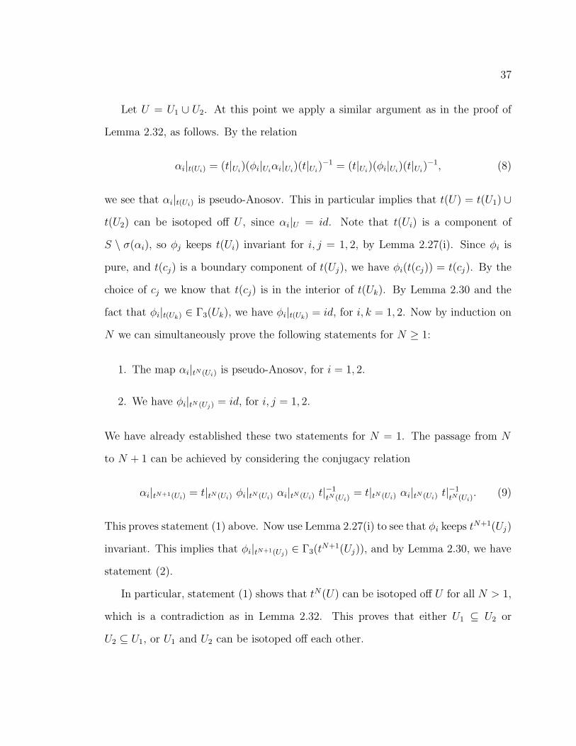
Let U = U1 ∪ U2. At this point we apply a similar argument as in the proof of
Lemma 2.32, as follows. By the relation
αi|t(Ui) = (t|Ui)(φi|Ui
αi|Ui)(t|Ui
)−1 = (t|Ui)(φi|Ui
)(t|Ui)−1, (8)
we see that αi|t(Ui) is pseudo-Anosov. This in particular implies that t(U) = t(U1) ∪
t(U2) can be isotoped off U , since αi|U = id. Note that t(Ui) is a component of
S \ σ(αi), so φj keeps t(Ui) invariant for i, j = 1, 2, by Lemma 2.27(i). Since φi is
pure, and t(cj) is a boundary component of t(Uj), we have φi(t(cj)) = t(cj). By the
choice of cj we know that t(cj) is in the interior of t(Uk). By Lemma 2.30 and the
fact that φi|t(Uk) ∈ Γ3(Uk), we have φi|t(Uk) = id, for i, k = 1, 2. Now by induction on
N we can simultaneously prove the following statements for N ≥ 1:
1. The map αi|tN (Ui) is pseudo-Anosov, for i = 1, 2.
2. We have φi|tN (Uj) = id, for i, j = 1, 2.
We have already established these two statements for N = 1. The passage from N
to N + 1 can be achieved by considering the conjugacy relation
αi|tN+1(Ui) = t|tN (Ui) φi|tN (Ui) αi|tN (Ui) t|−1tN (Ui)
= t|tN (Ui) αi|tN (Ui) t|−1tN (Ui)
. (9)
This proves statement (1) above. Now use Lemma 2.27(i) to see that φi keeps tN+1(Uj)
invariant. This implies that φi|tN+1(Uj) ∈ Γ3(tN+1(Uj)), and by Lemma 2.30, we have
statement (2).
In particular, statement (1) shows that tN(U) can be isotoped off U for all N > 1,
which is a contradiction as in Lemma 2.32. This proves that either U1 ⊆ U2 or
U2 ⊆ U1, or U1 and U2 can be isotoped off each other.

38
Now without loss of generality, suppose that U1 ⊆ U2, but U1 is not isotopic to U2.
Then there exists a component c1 of ∂U1 such that c1 is not isotopic to a component
of ∂U2. By Lemma 2.27(i), αi keeps U1 and U2 invariant for i = 1, 2. Also, by
Lemma 2.27(ii), αi(c1) = c1, which implies αi|U2= id, by Lemma 2.30. Again, using
(8) we get statement (1) for N = 1. Hence t(Ui) is a component of S \ σ(αi). So φi
keeps Uj invariant. Thus φi(t(c1)) = t(c1), which gives φi(U2) = id, by Lemma 2.30.
This proves statement (2) for N = 1. The passage from N to N + 1 follows by using
equation (9) above. Then again we have that U2 can be isotoped off tN(U2) for all
N > 1, which is a contradiction. This proves that U1 is isotopic to U2.
Lemma 2.34 Let U be a component of both S \ σ(φ1) and S \ σ(φ2) such that φi|U
is pseudo-Anosov for i = 1, 2. Then φ1|U commutes with φ2|U .
Proof. If φ1|U and φ2|U do not commute, then their centralizers in Γ3(U) have triv-
ial intersection by Corollary 2.31. This implies that αi|U = id, which contradicts
Lemma 2.32.
We are finally ready to prove Theorem B.
Proof of Theorem B. Let U be a component of S \σ(φ1) such that φ1|U is pseudo-
Anosov. We first prove that φ2|U is either pseudo-Anosov or the identity. Suppose
φ2|U is neither pseudo-Anosov nor the identity (in particular, U is not a component
of S \ σ(φ2)). Let V1, V2, · · · , Vs be components of S \ σ(φ2), which cover U up to
isotopy. We can assume that the cover is minimal in the sense that none of the Vk
can be isotoped off U . By Lemma 2.33, φ2|Vk= id for all 1 ≤ k ≤ s. (This does not
39
mean that φ2|U = id, since φ2 may involve Dehn twists about boundary components
of Vk.) By Lemma 2.29, i(∂U, ∂Vk) = 0 for all 1 ≤ k ≤ s, which shows that φ2
keeps U invariant. Moreover, φ2|U is a non-trivial composition of Dehn twists about
disjoint simple closed curves. Using Lemma 2.27(i), αi keeps U invariant. Since
αi|U , φj|U ∈ Γ3(U) and αi|U commutes with φ2|U , using Lemma 2.30 we see that αi|U
cannot be pseudo-Anosov. Moreover, αi|U commutes with φ1|U so αi|U = id. Now by
Lemma 2.32, we get that the centralizers of φ1|U and φ2|U must intersect non-trivially.
Lemma 2.30 then implies that φ2|U is either pseudo-Anosov or the identity, which is
a contradiction.
We have proved that for a component U of S \σ(φ1) where φ1|U is pseudo-Anosov,
φ2|U is either pseudo-Anosov or the identity. In the case that φ2|U is pseudo-Anosov,
φ1|U and φ2|U commute by Lemma 2.34. Similarly, for a component V of S \ σ(φ2)
where φ2|V is pseudo-Anosov, φ1|V is either a commuting pseudo-Anosov or the iden-
tity.
Let S1 be the subsurface of S which is the union of subsurfaces T such that either
φ1|T or φ2|T is pseudo-Anosov. We have proved that φ1 and φ2 both keep S1 invariant,
and φ1|S1commutes with φ2|S1
.
On S2 = S \ S1 both φ1 and φ2 are compositions of Dehn twists about disjoint
curves, by Lemma 2.29. Hence φ1|S2and φ2|S2
commute. We conclude that φ1 and
φ2 commute, contradicting part (1) of Theorem 2.22. This shows that FP-groups do
not embed inMg,b,n, as desired.

40
3 Winding Number and Representations of Map-
ping Class Groups
First Morita, then Trapp, and more recently Perron, all construct representations of
the mapping class group, each using very different techniques. These three separate
approaches, however, yield closely connected representations of Mg,1,0. The three
authors are probably aware of this fact (Trapp and Perron each credit Morita), yet the
precise connections amongst the three representations have not been made explicit.
Our goal in this section is to clarify these connections and hence to fill in a perceived
gap in the literature by presenting all three together as different interpretations of
what is essentially one representation.
Throughout this section we are only interested inMg,b,n in the case where n = 0,
and so we let Mg,b denote Mg,b,0, and likewise for any corresponding surfaces and
subgroups. Also, whenever we have need to make reference to a homology basis, we
will consider the standard symplectic basis used in both [20] and [46]. For reasons
which will become clear later, we now denote the symplectic representation of Mg,1
by ρ2 : Mg,1 → Sp(2g,Z). Recall that ρ2 records the action of the mapping class
group on homology, and its kernel is the Torelli group, Ig,1.
After presenting some necessary background, we describe Morita’s representa-
tion ρ3, which generalizes both the symplectic representation ρ2 as well as Johnson’s
crossed homomorphism τ : Ig,1 → Λ3H1(Sg,1,Z). We focus on a crossed homo-
morphism induced by Morita’s representation, which will serve as an important link
between Morita’s representation and that of Trapp and of Perron.

41
3.1 Group Cohomology Background
The cohomology of groups is usually defined using the language of cochain complexes.
It is more useful for our purposes to understand group cohomology in terms of crossed
homomorphisms, and therefore we follow Brown’s treatment of this subject in [8].
Let E be a group. We say that E is an extension of G by A, if we have a short
exact sequence
0→ A→ E → G→ 1
(though, as Brown notes, some authors, in particular Bernard Perron in [41], would
reverse the terminology and refer to this as an extension of A by G). For our purposes,
we will only need to consider the case where the kernel A is an abelian group (hence
the use of 0 on the left). An extension is split if we have a section s : G → E, or
equivalently, if E ∼= A o G. (Recall that the semi-direct product A o G is equal to
the set A×G together with multiplication given by (a, g) · (b, h) = (a+ gb, gh).)
There is a unique split extension corresponding to any given action of G on A.
However, there are possibly many different sections which induce the split exten-
sion. Let s : G → A o G be a section of a split extension. Then the induced map
onto the first factor s : G → A is necessarily a crossed homomorphism. A crossed
homomorphism (sometimes called a derivation) is a function d : G → A such that
d(gh) = d(g) + g d(h). Let Der(G,A) denote the set of all crossed homomorphisms
d : G → A. The set of possible sections of the given split extension is in 1-1 corre-
spondence with the set Der(G,A) [8].
We now introduce an equivalence relation on crossed homomorphisms, and hence
on sections, which will clarify our use of the word “unique” in the previous paragraph.
Let a ∈ A, and define a crossed homomorphism da : G → A by da(g) = ga − a.

42
Then we will say that d1 ∼ d2 if d2 − d1 = da for some a ∈ A. Such a function
da is called a coboundary or a principal derivation. Denote by P (G,A) the set of
all such coboundaries. We define the first cohomology of G with coefficients in A,
denoted H1(G,A), as Der(G,A)/P (G,A). The corresponding notion of equivalence
for sections is simply conjugation, i.e., if a ∈ A, and i(a) represents the inclusion of
a in AoG, then two sections s1 and s2 are equivalent if there exists an a ∈ A which
satisfies s1(g) = i(a)s2(g)i(a)−1 for all g ∈ G [8].
There is another interpretation of H1(G,A) which will also be useful to us in
the case of mapping class groups. Thus we now follow Morita’s treatment of group
cohomology in [37] in the special case where G = Mg,1 and A = H1(Sg,1;Z) (we
will usually drop the Z from this notation, but it is to be understood). We know
that Mg,1 acts on H1(Sg,1) via the symplectic representation ρ2, and we will de-
note this by φ∗(x) = ρ2(φ)(x). If we employ the usual identification of H1(Sg,1)
with Hom(H1(Sg,1),Z), we can describe the action of Mg,1 on H1(Sg,1) by φu(x) =
u(φ−1∗
(x)) = u(ρ2(φ−1)(x)) for φ ∈ Mg,1, u ∈ H
1(Sg,1), and x ∈ H1(Sg,1).
Let F (Mg,1×H1(Sg,1),Z) denote the set of all functions f :Mg,1×H1(Sg,1)→ Z
such that:
1. f(φ, x+ y) = f(φ, x) + f(φ, y)
2. f(φψ, x) = f(φ, ψ∗(x)) + f(ψ, x)
Let d ∈ Der(Mg,1;H1(Sg,1)), and let fd : Mg,1 × H1(Sg,1) → Z be given by
fd(φ, x) = d(φ−1)(x). We have a bijection given as follows:
Der(Mg,1;H1(Sg,1)) ←→ F (Mg,1 ×H1(Sg,1),Z)
d ←→ fd (10)

43
In view of this fact, Morita also refers to elements of F (Mg,1×H1(Sg,1),Z) as crossed
homomorphisms. Let a ∈ H1(Sg,1;Z). Then the bijection carries the coboundary
da ∈ Der(Mg,1;H1(Sg,1;Z)) to a map da :Mg,1 ×H1(Sg,1),Z) defined by da(φ, x) =
a(φ∗(x) − x). Here we follow Morita in abusing notation by retaining the name da,
and we will also refer to such maps as coboundaries. Thus another way to interpret
H1(Mg,1;H1(Sg,1)) is as the set F (Mg,1 ×H1(Sg,1),Z) modulo coboundaries.
3.2 Morita’s Representation ρ3
Let π denote the fundamental group of the surface Sg,1, and let π′ denote its com-
mutator subgroup. Also, we will use H1 as a shorthand notation for the first integral
cohomology group of Sg,1, and H1 to denote the first integral homology group. By
Poincare duality we have H1 ∼= H1, so we will often simply use H when it is unneces-
sary to be more specific. Johnson constructs homomorphism τ : Ig,1 → Λ3H in [20]
based on the action of Mg,1 on the quotient π/[π, π′]. Morita generalizes Johnson’s
approach to the extent of finding a sequence of representations ofMg,1 based on its
action on the lower central series of the fundamental group of the surface Sg,1 in [39].
We denote the lower central series by Γj. Thus Γ1 = π1(Sg,1), and Γj+1 = [Γ1,Γj]
for j ≥ 1. The quotient group Nj = Γ1/Γj is known as the j-th nilpotent quotient of
Γ1. Note that N2 is just H, the first integral homology of Sg,1. Now if we fix a base
point on the boundary of our surface,Mg,1 acts naturally on the fundamental group
Γ1. This action induces an action on each nilpotent quotient Nj, which then yields a
sequence of representations ρj :Mg,1 → Aut N3. Since N2 = H, ρ2 is just the sym-
plectic representation of the mapping class group, and Im ρ2 = Sp(H) ∼= Sp(2g,Z).
We would like to develop a similarly useful understanding of Im ρ3. “Useful” here

44
means that we can embed the image in a semi-direct product, each factor of which is a
piece which we can interpret geometrically and connect to our other representations.
Morita outlines this process very carefully in [39], and we follow his exposition here.
Though we do not give every detail, we aim to describe Morita’s construction well
enough that the reader will be able to compare his methods to those of Trapp and
Perron. We will incorporate most of Morita’s notation and terminology so that the
interested reader will have an easier time reading the more detailed version in [39].
Let Ij = ρj(Ig,1), and let I(Nj) denote the subgroup of Aut Nj whose elements
act trivially on the first homology of Nj. Morita first shows that Ij is an extension of
Sp(H) by I(Nj). Unfortunately, this extension is not split. Morita determines that
Aut Nj is an extension of GL(H) by I(Nj) (each of which contains an embedded copy
of its respective counterpart above), but again this extension is not split.
Morita turns to the Mal’cev completion of a nilpotent group (see [34] for the
definition) and considers a new representation ρj ⊗Q :Mg,1 → Aut (Nj ⊗Q). The
case k = 3 is special because there is an explicit product description for the Mal’cev
completion N3 ⊗ Q. Namely, N3 ⊗ Q ∼= Λ2HQ × HQ, where HQ = H ⊗ Q, with
multiplication defined by (ξ, u)(η, v) = (ξ+η+ 12u∧v, u+v). We skip over the details,
but this product description ultimately enables Morita to give a split extension.
0→ Hom(HQ,Λ2HQ)→ Aut (N3 ⊗Q)→ GL(HQ)→ 1
where the action of GL(HQ) on Hom(HQ,Λ2HQ) is given by (Af)(u) = Af(A−1u)
for A ∈ GL(HQ), f ∈ Hom(HQ,Λ2HQ), and u ∈ HQ.
For any split extension, the projection map from the semi-direct product onto
its first factor is necessarily a crossed homomorphism (see [8] or [17]). Let q :
Aut (N3 ⊗Q) → Hom(HQ,Λ2HQ) be the crossed homomorphism associated to the

45
split extension Aut (N3⊗Q) ∼= Hom(HQ,Λ2HQ)oGL(HQ) given above. For simplic-
ity, let r = ρ3⊗Q. If we compose q with the representation r :Mg,1 → Aut (N3⊗Q),
we obtain another crossed homomorphism k :Mg,1 → Aut (N3 ⊗Q), which Morita
calls the crossed homomorphism associated to r. Since Hom(HQ,Λ2HQ) becomes an
Mg,1-module via the symplectic representation ρ2, we can express the fact that k is
a crossed homomorphism as follows:
k(φψ) = k(φ) + ρ2(φ)k(ψ).
In addition, we can use the semi-direct product structure of Aut (N3 ⊗Q) to write
r(φ) = (k(φ), ρ2(φ)) for any φ ∈ Mg,1.
We now return our attention to the group Aut N3 and the representation ρ3.
Again, building on special properties of the Mal’cev completion of the nilpotent quo-
tients Nj in the case j = 3, Morita is able to show that there exists an embedding
i : N3 → N3 ⊗ Q which induces an injection i∗ : Aut N3 → Aut (N3 ⊗ Q) such
that r = i∗ ◦ ρ3. Thus Im r ∼= Im ρ3, and we have a copy of Im ρ3 embedded in
Aut (N3 ⊗Q) ∼= Hom(HQ,Λ2HQ) o GL(HQ).
Using the respective natural embeddings of Λ2H andH into Λ2HQ andHQ, Morita
shows that Im ρ3 ⊆ Hom(H, 12Λ2H) o Sp(H) [39]. We will follow Morita’s abuse of
notation and also use the symbol k to denote the crossed homomorphism associated
to ρ3.
We must now examine the dependence of the above construction on the injection
i. A different embedding of N3 in N3 ⊗ Q may change our embedding of Imρ3
in Aut (N3 ⊗ Q). Suppose that i′ : N3 → N3 ⊗ Q were another such injection.
Then Morita shows in [39] that there exists an element f ∈ Hom(HQ,Λ2HQ) ⊂
Aut (N3⊗Q) such that i′ = f ◦ i. Each i′ induces a representation r′ = i′∗◦ρ3 with an

46
associated crossed homomorphism k′ :Mg,1 → Hom(HQ,Λ2HQ). Then the following
equation holds for all φ ∈ Mg,1:
k′(φ) = k(φ) + f − ρ2(φ)f.
But according to our previous notation from Section 3.1, f − ρ2(φ)f is just the
coboundary d(−f). If we denote this coboundary by δf , we can write simply that
k′ = k + δf . We shall call k′ the crossed homomorphism associated to the map f . In
other words, any two crossed homomorphisms arising from such a construction will
differ by a coboundary and hence are identical as elements of cohomology.
Remark 3.1 There are some technical details which are being glossed over here. By
referring to i′ as “another such injection”, we mean that N3 is an extension of H by
Λ2H, N3⊗Q is an extension of HQ by Λ2HQ, and the injection i′ : N3 → N3⊗Q must
make the short exact sequences corresponding to these extensions commute with the
natural inclusions of Λ2H and H into Λ2HQ and HQ, respectively.
We can now adjust the image of our crossed homomorphisms within Hom(HQ,Λ2HQ)
(and hence the image of ρ3 within Hom(HQ,Λ2HQ)oSp(H)) simply by choosing dif-
ferent maps f . In [39], Morita explicitly constructs a map f ∈ Hom(H, 12Λ2H) with
the property that Im(k + δf) ⊂12Λ3H ⊂ Hom(H, 1
2Λ2H). In yet another abuse of
notation, we denote by k the crossed homomorphism associated to this particular
map f . We are now in a position to write down the representation ρ3 in such a way
that Im ρ3 is useful to us.
Theorem 3.2 (Morita, [39]) Let k :Mg,1 →12Λ3H be the crossed homomorphism
associated to the map f given above. Then we can embed Im ρ3 into 12Λ3H o Sp(H)

47
and the representation ρ3 can be described explicitly by the formula
ρ3(φ) = (k(φ), ρ2(φ))
for any φ ∈ Mg,1. Furthermore, the restriction of the crossed homomorphism k to
the Torelli group Ig,1 is precisely Johnson’s homomorphism τ : Ig,1 →12Λ3H.
Note that Johnson defined his map τ with values in Λ3H, so we make the obvi-
ous identification. The map τ carries some interesting geometric information about
mapping classes in Ig,1 [22], and we shall see that k carries the same information for
all ofMg,1.
3.3 Crossed Homomorphisms Mg,1 → H
Using calculations involving projections of π1(Sg,1) onto F2, Morita constructs a
crossed homomorphism k : Mg,1 × H1(Sg,1) → Z [37]. He proceeds to show in
[39] that k is the contraction of the crossed homomorphism k : Mg,1 →12Λ3H. In
other words, if we let C : Λ3H → H be the standard contraction map given by
C(x ∧ y ∧ z) = 2[(x · y)z + (y · z)x + (z · x)y]
where · denotes the intersection pairing of homology classes, then k = C ◦ k :Mg,1 →
H. From either point of view, Morita’s constructions of the crossed homomorphism
k are purely algebraic. Since we will actually be more concerned with the contraction
of k, we understand “Morita’s representation” to refer to the map ρ3 composed with
contraction of the first factor.
However, we know that k restricts to Johnson’s homomorphism τ . We now de-
scribe the geometric information carried by τ . Johnson proves in [22] that C ◦ τ is

48
what is known as the Chillingworth homomorphism of Ig,1, which records how a given
element of the Torelli group acts on the winding number of curves on a surface, a
concept introduced by Chillingworth in [9]. Let X be a nonsingular vector field on
Sg,1. If γ is an oriented, direct, regular curve on Sg,1, then its winding number relative
to X, denoted ωX(γ), is the number of times the tangent vector to the curve rotates
relative to the vector field X (for more details see [9]).
Remark 3.3 Chillingworth’s winding number function is well-defined on homotopy
classes and for technical reasons must be computed using a representative curve which
is both regular and direct. We recall that a curve is regular if continuously varying
non-zero tangents exist at all points of the curve. A closed curve which self-intersects
transversally finitely many times is said to be direct if it contains no nullhomotopic
loop.
Remark 3.4 We note two interesting facts about winding numbers of curves on
surfaces:
1. Formula 1 of [9] shows how the winding number of any homotopy class is de-
termined by the winding numbers of a particular basis of π1(Sg,1).
2. Let γ1, . . . , γ2g be a basis of π1(Sg,1). Then Theorem 4.2 of [9] points out that
a non-vanishing vector field X can be chosen to satisfy any given assignments
ωX(γi) = ai, ai ∈ Z.

49
Following Trapp ([46]), we define a function eX :Mg,1 → H1 given by eX(f)(γ) =
ωX(f(γ)) − ωX(γ). This function measures the change in winding numbers of our
homology basis effected by a given element of the mapping class group relative to a
fixed vector field X. Johnson first defined such a function on the Torelli group in [20].
Remark 3.5 In general, winding numbers are not well defined on homology classes,
but Trapp shows in [46] that eX(f) is actually well defined on homology classes for
all f ∈ Mg,1. (An argument in the restricted case of Ig,1 is also given in [20].) Note
that we will often abuse notation by referring to both the curve and its homology
class as γ. Since H1 ∼= Z2g, we will think of elements in H1 as row vectors.
The function eX is not a homomorphism on the entire mapping class group, but it
is a crossed homomorphism in the sense that it obeys the following composition law
(as proved in [46]):
eX(fh) = eX(f)ρ2(h) + eX(h). (11)
It is easy to check that Trapp’s map eX : Mg,1 → H1 is a also crossed ho-
momorphism in the sense of Morita. We will view eX as an element of the set
F (Mg,1 × H1(Sg,1),Z). In this case, we need to check the two criteria set forth by
Morita. The first is clear. To check the composition law, let f, h ∈ Mg,1, and let
x ∈ H1. Then what we need to show is that
eX(fh)(x) = eX(f)(h∗x) + eX(h)(x) (12)
= eX(f)ρ2(h)(x) + eX(h)(x)

50
since the action ofMg,1 on H1 is given by the symplectic representation. But this is
precisely the criterion described in Equation11.
In any case, it is immediately clear that eX is a homomorphism when restricted to
the Torelli group. Johnson proves this directly in [20]. It is worth noting that we also
have from Johnson the fact that eX is independent of the choice of the vector field
X when restricting to Ig,1. In particular, in the restricted case we can write e(f) or
ef for eX(f) and dualize to a homology class t(f) determined by intersection pairing:
γ · t(f) = ef(γ); Johnson refers to t(f) as the Chillingworth class of f . Then we can
think of t as a homomorphism from the Torelli group to H, which we will call the
Chillingworth homomorphism. Thus, from our previous discussion, we can now write
C ◦ τ = t.
Using the map k described at the beginning of Section 3.3, Morita establishes that
crossed homomorphisms of the formMg,b → H are essentially unique.
Theorem 3.6 (Morita, [37]) H1(Mg,1;H1(Sg,1)) ∼= Z, with generator k.
Combining Theorem 3.6 with Theorem 3.2, we have therefore established that the
Chillingworth homomorphism t extends essentially uniquely to the full mapping class
group (up to coboundary and sign). More precisely, thinking of eX as the extension
of t toMg,1, we have:
Proposition 3.7 k = eX , as elements of H1(Mg,1;H1(Sg,1)).
We note that Theorem 6.1 of [38] is the special case of Proposition 3.7 when the
crossed homomorphisms are restricted to Ig,1, and that the proof utilizes the bijection
given in Equation 10.

51
We have established that Trapp’s crossed homomorphism eX which measures the
action of a mapping class on winding numbers is essentially equal to Morita’s crossed
homomorphism k, a fact first realized by Trapp in [46]. The result here is not new,
since both Trapp and Morita realized that the Chillingworth homomorphism extended
to the entire mapping class group, and Trapp realized that his crossed homomorphism
was “essentially” the same as Morita’s. Besides pinning down the connections, our
goal is to see the geometric interpretation of each representation. What Morita does
not explicitly state is that k carries winding number information not only for the
Torelli group, but for the whole mapping class group. Thus it is possible to extract
this winding number information directly from Morita’s representation.
3.4 Trapp’s Representation
Trapp uses his crossed homomorphism eX to construct a linear representation TX :
Mg,1 → GL(2g + 1,Z) given as follows:
TX(f) =
(1 eX(f)0 ρ(f)
)
where X is a given nonsingular vector field on Sg,1. We again let ρ : Mg,1 →
Sp(2g,Z) denote the symplectic representation, dropping the index 2 introduced for
other purposes in Section 3.2. The 0 in the matrix denotes a column of 2g zeros.
We note that Trapp’s representation can be factored through Mg,0, though we do
not address it here, and that Patricia Sipe previously discovered this version of the
representation in [44].
Remark 3.8 Until now, we have ignored the issue of the choice of the vector field X.
Trapp proves that eX does not depend on X when restricting to Ig,1, and moreover,

52
that if X and X ′ are different vector fields on Sg,1, then TX and TX′ are conjugate
representations. We henceforth denote the above representation simply by T . It fol-
lows from Morita’s work that outside of Ig,1, different choices of X should correspond
to varying the crossed homomorphism k by a coboundary.
Trapp’s definition of this representation is particularly nice because it interprets
Morita’s purely algebraic constructions explicitly in terms of geometry, and also be-
cause it linearizes Morita’s representation. Trapp also proves that T (f) can be un-
derstood to measure the acton of Df on the first homology with Z coefficients of the
unit tangent bundle of the surface (Theorem 2.2, [46]).
We claim that Im T is a split extension of Sp(2g,Z) by 2H ∼= H. If π : Im T →
Sp(2g,Z) is the obvious map which picks out the 2g×2g lower right-hand block, then
we have the following short exact sequence
0 −→ ker π −→ Im T −→ Sp(2g,Z) −→ 1.
The splitting is given in the obvious way, by sending a matrix A ∈ Sp(2g,Z) to the
matrix(
1 00 A
)
.
Also, Proposition 2.8 of [46] tells us that ker π ∼= 2H, which establishes our claim.
Trapp addresses the issue of splittings only in the case where he factors T through
Mg,0.

53
3.5 Perron’s Representation
We now describe a completely different approach to the linearization of Morita’s
representation given by Bernard Perron in [41].
To any graph Γ we will associate a particular Artin group, denoted A(Γ). To each
vertex of Γ we associate a generator of A(Γ), and we shall abuse notation by using
the same symbol to denote both. If x and y are two vertices of Γ bounding a common
edge, then the corresponding generators “braid”, that is, xyx = yxy. If no such edge
exists, then x and y commute.
Remark 3.9 As noted, we are only concerned here with one specific kind of Artin
group, but the reader is probably familiar with a much more general construction.
There are different conventions for using Coxeter graphs to present an Artin group.
Here we take the definition used in [10]. A Coxeter graph consists of vertices and
labelled edges, with edge labels taken from the set {3, 4, . . . ,∞}. Then the associ-
ated Artin group has a presentation in which generators correspond to vertices, and
relations correspond to edges as follows. If s, t are vertices bounding a common edge
with label ms,t, then we have the relation ststs · · · = tstst · · ·, where the word on each
side of the equation has length ms,t. If ms,t = ∞, there is no relation. If s, t do not
bound a common edge, then we have the relation st = ts. In our case, then, any edge
in our graph would have the label 3, corresponding to the braid relation sts = tst.
Hence, for simplicity in this special case, we are simply dropping the labels.
Example 3.10 Let An be the graph in Figure 3. Then A(An) = Bn+1, where Bk

54
σ1 σ2 σ3 σp σn−1 σn
������������ ���� ���� ������������ ��������
� � � � � ����������� �� �������� ������������������������������ ����������
Figure 3: The graph An
σ1 σ2 σ3 σp σn−1 σn
δ
������������ �� !!"" #�##�#$�$$�$ %%&& '�''�'((
)�))�)*�**�*
+�+�+�+�+�+,�,�,�,�,�, -. /01�12�2 3�34�45�5�5�56�6�6�67�7�78�8�8 9�9�9:�:�:;;;;;;
<<<<<<
Figure 4: The graph En+1,p
denotes the braid group on k strands.
The graph An embeds in the graph En+1,p shown in Figure 4. This inclusion
induces an injection on the corresponding groups: Bn+1 → A(En+1,p) [41]. The
connection to mapping class groups comes when we let n = 2g and p = 4, for
Matsumoto has given Mg,1 explicitly as a quotient of A(E2g+1,4) [34].
This connection between A(En+1,p) andMg,1 is easy to see if we look at Humphries’
generating set forMg,1, which consists of Dehn twists about the curves shown in Fig-
ure 5. Recall that Dehn twists about disjoint curves will commute and that Dehn
twists about curves which intersect once will braid. Then each vertex σi ∈ A(E2g+1,4)
naturally corresponds to the Dehn twist about the curve Ci, and δ corresponds to the
second meridian curve B. Hence Perron’s strategy is to begin with a representation
of the braid group, extend it to A(En+1,p), and then factor it throughMg,1.
Perron begins with the well-known (reduced) Burau representation

55
C1 C3 C5C2 C4 C6 C2g
B
Figure 5: Humphries’ generating set for π1(Sg,1)
Bn+1 → GLn(Z[t, t−1]), defined as follows:
σi 7→ Ji =
Ii−2 0 0
01 0 0t −t 10 0 1
0
0 0 In−i−1
,
where Ik stands for the k × k identity matrix. We note that in the case i = 1, n, we
have, respectively:
σ1 7→ J1 =
−t 10 1
0
0 In−2
, σn 7→ Jn =
In−2 0
01 0t −t
.
The problem is that the Burau representation does not extend to A(En+1,p) when
p = 4. Therefore Perron extends the Burau representation slightly. Let Ri denote an
n × n block of zeros with a t placed in the (i, i)th position. It is easy to check that
the map
Bn+1 → GL2n(Z[t, t−1])
σi 7→
(In 0Ri Ji
)

56
is a well-defined representation, which Perron refers to as the Burau bis representation.
The Burau bis representation extends to A(En+1,p) for all possible values of n and
p, in the following way. Let ~b =
b1···bn
, ~d =
d1
···dn
, and λ = (λ1, . . . , λn). We
define the following n× n matrices:
A =(
λ1~b λ2
~b · · · λn~b
)
B =(
~0 · · · ~0 ~b ~0 · · · ~0)
C =(
λ1~d λ2
~d · · · λn~d
)
D =(
~0 · · · ~0 ~d ~0 · · · ~0)
,
where ~0 denotes a column of n zeros. Let us further assume that the bi, i = 1, . . . , n
satisfy the following conditions:
tbi = −tdi−1 + (1 + t)di − di+1, i 6= p
tbp = −tdp−1 + (1 + t)dp − dp+1 + tn∑
i=1
λibi = −(1 + dp + t),
setting any undefined dj equal to zero. If we make the assignments
σi 7→
(In 0Ri Ji
)
δ 7→
(In + A BC In +D
)
,
then for each choice of λ, we get a linear representation ψλ : A(En+1,p) → GL2n(R),
where we can take R to be the field of rational fractions in n + 1 indeterminates
Q(t, d1, . . . , dn) (Proposition 2.2 of [41]). Perron then shows that one can obtain a
representation ofMg,1 by making choices for t and λ.
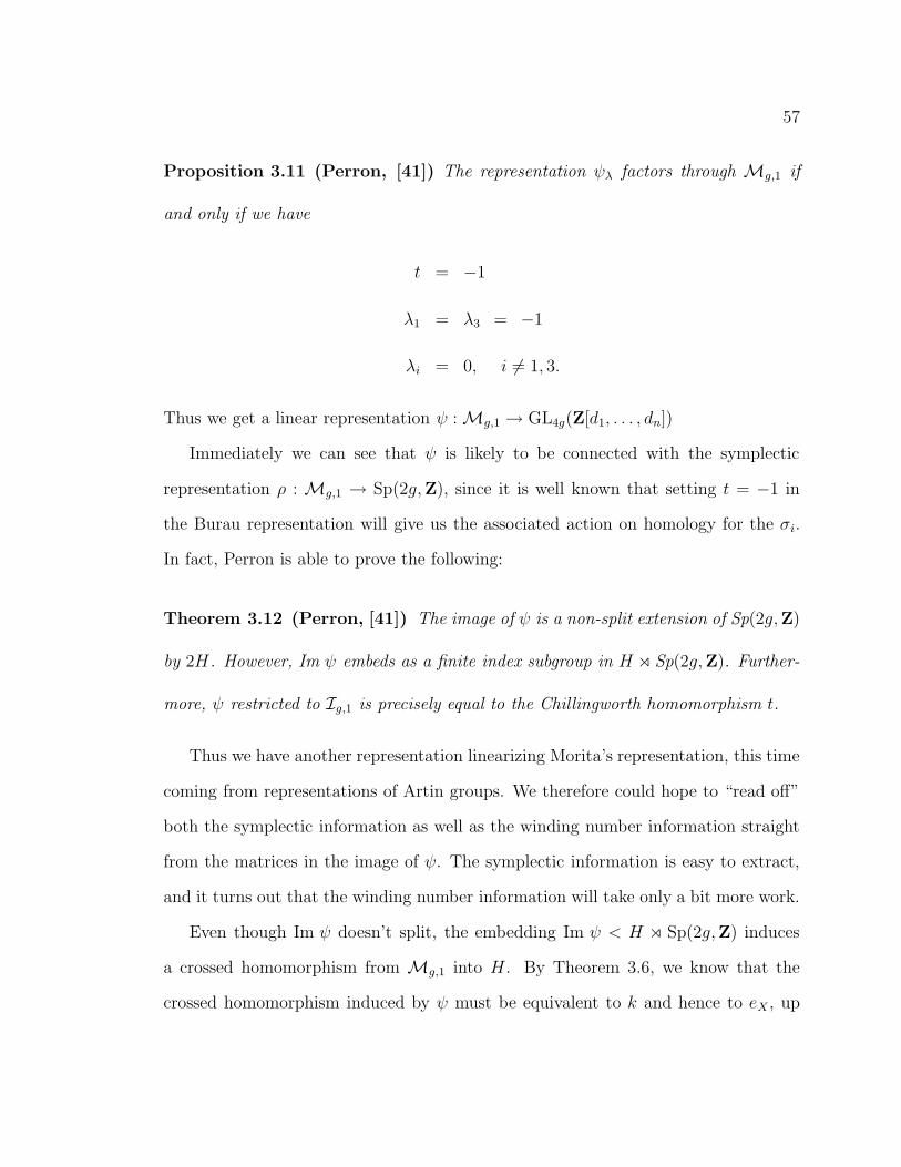
57
Proposition 3.11 (Perron, [41]) The representation ψλ factors through Mg,1 if
and only if we have
t = −1
λ1 = λ3 = −1
λi = 0, i 6= 1, 3.
Thus we get a linear representation ψ :Mg,1 → GL4g(Z[d1, . . . , dn])
Immediately we can see that ψ is likely to be connected with the symplectic
representation ρ : Mg,1 → Sp(2g,Z), since it is well known that setting t = −1 in
the Burau representation will give us the associated action on homology for the σi.
In fact, Perron is able to prove the following:
Theorem 3.12 (Perron, [41]) The image of ψ is a non-split extension of Sp(2g,Z)
by 2H. However, Im ψ embeds as a finite index subgroup in H o Sp(2g,Z). Further-
more, ψ restricted to Ig,1 is precisely equal to the Chillingworth homomorphism t.
Thus we have another representation linearizing Morita’s representation, this time
coming from representations of Artin groups. We therefore could hope to “read off”
both the symplectic information as well as the winding number information straight
from the matrices in the image of ψ. The symplectic information is easy to extract,
and it turns out that the winding number information will take only a bit more work.
Even though Im ψ doesn’t split, the embedding Im ψ < H o Sp(2g,Z) induces
a crossed homomorphism from Mg,1 into H. By Theorem 3.6, we know that the
crossed homomorphism induced by ψ must be equivalent to k and hence to eX , up

58
to an integer multiple. Therefore the winding number information must somehow be
contained in Morita’s representation. The last statement in Theorem 3.12 tells us
where to look for it.
We recall that Im ψ < GL4g(Z[d1, . . . , dn]). Let ρ : Im ψ → Sp(2g,Z) be the map
defined by extracting the lower right-hand 2g × 2g block from the matrix and by
setting d1 = d3 = 1 and di = 0 for i 6= 1, 3. Then Perron shows that the following
diagram of short exact sequences commutes, and thus application of ρ yields the
symplectic data.
1 Ig,1 Mg,1 Sp(2g,Z) 1
0 2H Im ψ Sp(2g,Z) 1
-
-
-
-
-
-
-
-
? ? ?
t ψ id
i
ξ
ρ
ρ
If we want to understand how winding number information is contained in the
representation ψ, we must therefore understand the injection ξ : H → Im ψ. For an
explicit definition of ξ, see [41]. For our purposes, it suffices to know that for m ∈ H,
ξ(m) has the form
(
N1 m~bN2 N3
)
, where the Ni are 2g×2g blocks, ~b is a column vector
of indeterminates dependent upon the di as previously defined, and m~b denotes the
2g × 2g matrix
(
m1~b · · · m2g
~b)
=
m1b1 · · · m2gb1m1b2 · · · m2gb2
......
m1b2g · · · m2gb2g
.
Let us now examine exactly how Im ψ embeds in H o Sp(2g,Z). Let δ∗ denote

59
j
Figure 6: The involution j
the image under ψ of the Dehn twist about the curve j(B), where j is rotation
by π about the axis indicated in Figure 6. Let 〈Im ψ, δ∗〉 denote the subgroup of
GL4g(Z[d1, . . . , dn]) generated by Im ψ and δ∗. Following Perron, we can extend the
map ρ : Im ψ → Sp(2g,Z) to a map ρ′ : 〈Im ψ, δ∗〉 → Sp(2g,Z) by setting
ρ′(δ∗) =
1 0 0 10 1 0 10 0 1 10 0 0 1
0
0 I2g−4
.
Then it follows from Proposition 8.10 of [41] that we have another commutative
diagram of exact sequences.
0 2H Im ψ Sp(2g,Z) 1
0 H 〈Im ψ, δ∗〉 Sp(2g,Z) 1
-
-
-
-
-
-
-
-
? ? ?
incl incl id
ξ
ξ
ρ
ρ′
The lower sequence splits, and hence the above gives us the embedding of Im ψ
in a semidirect product, as previously mentioned. The corresponding section S :

60
Sp(2g,Z)→ 〈Im ψ, δ∗〉 is given by
S(A) =
(Ig 0RA A
)
.
The g× g matrix RA is not relevant to our calculations; an explicit definition can be
found in [41]. Any element in H o Sp(2g,Z), and hence any element in Im ψ, can
be written uniquely as a product ξ(m)S(A) for some m ∈ H (actually, m ∈ 2H) and
some matrix A ∈ Sp(2g,Z). Since the crossed homomorphism induced by ψ comes
from the first factor, and since the first pair of commuting exact sequences tells us
that ξ restricted to Ig,1 is precisely the Chillingworth homomorphism t, ξ(m) must
carry the winding number information. A simple calculation now tells us how to “see”
winding number information in Im ψ. Let Y ∈ Im ψ. Then
Y = ξ(m)S(A) =
(
N1 m~bN2 N3
) (Ig 0RA A
)
for some m ∈ H,A ∈ Sp(2g,Z). Multiplying this out tells us that any Y ∈ Im ψ is
of the form
Y =
(
N1 + (m~b)RA (m~b)AN2 +N3RA N3A
)
.
Since ξ is an injection, we might as well think of m as carrying the winding number
information. Then winding number information is actually embedded in many places
in this matrix, as m also appears in all the Ni. But the easiest place to see it is the
2g × 2g upper right-hand block. Since A ∈ Sp(2g,Z), A is invertible and m~b can be
calculated. To be more explicit, let ρ denote the process of setting d1 = d3 = 1 and
di = 0 for i 6= 1, 3. Therefore, if we have
ψ(f) =
(M1 M2
M3 M4
)
,

61
then we can compute
m~b = M3[ρ(A4)]−1.
By construction of the matrix m~b, we can then “read off” the vector m and the
winding number information contained therein.
Remark 3.13 We first note that Perron’s representation cannot be equivalent to
Trapp’s, since Im ψ does not split, but, like Morita’s, construction, only embeds in
a splitting. We also remind the reader that the vector describing winding number
will depend on some choice of vector field X. The reader will note that the upper
right-hand block in ψ(σi) is 0 by definition for all i = 1, . . . , 2g, and hence the winding
number vector will be the zero vector for each, a fact which may surprise the reader
(and indeed surprised the author). However, a careful application of Theorem 4.2 and
Formula 1 in [9] (see Remark 3.4) shows that indeed a vector field X can be found on
Sg,1 satisfying this condition. Moreover, the remaining generator ofMg,1 does effect
change on winding number, i.e., does not correspond to a zero block, and therefore
winding number is still “interesting” on the full mapping class group.
For the sake of completeness, we must also mention certain linear representations
of Artin groups found by Squier in [45]. As Trapp points out, his representation
T is precisely the case where Squier’s parameters satisfy a certain condition which
allows Squier’s map to factor through mapping class groups. In this context, then,
the connection between Trapp’s representation and Perron’s construction is not so
surprising.

62
In summary, therefore, we have described three representations ofMg,1, each aris-
ing in a very different context and employing vastly different methods of construction,
from Mal’cev completions to actions on tangent bundles to quotients of Artin groups.
The amazing fact is that each representation contains essentially the same informa-
tion. We hope that the above discussion has served the purpose of making explicit
the connections between these three representations, and, since the author has a bias
towards the geometric interpretation, we hope that it is now clear how the geomet-
ric information explicitly given in Trapp’s representation is encoded in Morita and
Perron’s representations. We also emphasize the important role played here by the
Torelli group, especially by Johnson’s map τ : Ig,1 → Λ3H, which motivates and lays
the groundwork for Morita’s original construction. An attempt to understand the
Torelli group better will make up the final section of this thesis.
Before closing Section 3, however, we make a few remarks concerning the po-
tential application of representations of mapping class groups to the classification
problem for Heegaard splittings of a given closed and orientable 3-manifold M . A
little background will be necessary at this point. A Heegaard splitting of M is a de-
composition of a 3-manifold into two handlebodies of genus g , F1 and F2, such that
F1 ∩ F2 = ∂F1 = ∂F2, and F1 ∪ F2 = M . We can also construct Heegaard splittings
by beginning with the two handlebodies and specifying a “gluing” homeomorphism
φ : ∂F1 → ∂F2, producing a 3-manifold M . We denote this as follows: M = F1∪φ F2.
Isotopic homeomorphisms yield homeomorphic 3-manifolds; thus we may simply spec-
ify the mapping class of φ inMg,0. Two Heegaard splittings of a given 3-manifold M
are equivalent if there exists an isotopy of M taking one splitting surface to the other.
We note that the gluing map is necessarily an element of Mg,0, while the previous

63
discussion focused on representations ofMg,1. However, each of the above represen-
tations factors through Mg,0, though the details were not relevant to our discussion
here.
Equivalence classes of Heegaard splittings correspond to double cosets in Mg,0
mod Hg,0, where Hg,0 denotes the handlebody subgroup, which is the subgroup of
Mg,0 consisting of mapping classes which extend to a homeomorphism of a fixed
handlebody whose boundary is the surface Sg,0. Invariants of these double cosets,
or of any homomorphic image of these double cosets, will be invariants of Heegaard
splittings. For example, Birman found invariants of Heegaard splittings arising from
double cosets under the symplectic representation [5].
The process of adding a trivial “handle” to a Heegaard splitting is known as
stabilization. In other words, we add a 1-handle to each handlebody and glue them by
mapping the longitude of one to the meridian of the other. It is known that given any
two Heegaard splittings of any 3-manifold M , only a finite number of stabilizations
are required before the two splittings become equivalent. In fact, there are no known
examples in which more than one stabilization is necessary. The obvious question to
ask is then, does it only require one stabilization in general to render two inequivalent
splittings equivalent?
Birman’s invariant has one crucial shortcoming. It is always trivial on a stabilized
Heegaard splitting. A new, better invariant, would almost certainly shed light on the
second question raised above. Fascinating examples have been developed recently by
Moriah and separately by Menasco which may provide counterexamples, but these
examples must wait for an invariant.
In order to calculate invariants of these double cosets under some representation,

64
one must first understand the image of Hg,0. Birman’s success in using the symplec-
tic representation to develop invariants of Heegaard splittings comes from the fact
that ρ(Hg,0) has a simple, algebraic description which lends itself to calculations.
Unfortunately, in general, the image of Hg,0 is quite difficult to characterize, but a
thorough study of Ig,0 might be of use here. For example, the Trapp/Sipe repre-
sentation is an excellent candidate for obtaining a “nice” image of Hg,0, since, after
all, it is a quotient of the symplectic representation together with one extra row of
winding number data. One can nearly characterize double cosets mod Hg,0 under the
Trapp/Sipe representation, but one cannot complete the calculation without knowing
Hg,0 ∩ Ig,0. Given the important role frequently played by the Torelli group in other
representations, one suspects the similar information would eventually be necessary
in calculating double cosets there as well.

65
4 Relations in the Torelli Group
Obtaining information about the mapping class group of a surface from its known
representations is a difficult problem, so we now turn our attention to one of the
most important subgroups of the mapping class group, namely, the Torelli group.
We continue with the notation of Section 3 by letting Sg,b denote Sg,b,0, with similar
notation for the corresponding mapping class groups and Torelli groups.
Powell gave an infinite set of generators of the Torelli group consisting of two
kinds of maps [42]. The first type are so-called bounding pair maps (BP-maps for
short). Let Tγ denote a Dehn twist about a curve γ. A BP-map is a product of
Dehn twists TαT−1β , where the curves α and β are each non-separating but together
bound a subsurface. The second type are commonly called BSCC-maps, short for
bounding simple closed curves. It is interesting to note that the subgroup of Ig,1
generated by BSCC-maps is precisely the kernel of Johnson’s homomorphism τ [24].
However, it is BP-maps which play the key role in generating Ig,1. Johnson was able
to show in [26] that BP-maps whose curves bound a genus 1 subsurface generate Ig,0
and Ig,1 for g ≥ 3 (again, an infinite set), before proving in [22] that a certain finite
set of BP-maps of various genus would suffice (thus settling a problem first raised
in Kirby’s problem list [28]). The question of whether the Torelli group is finitely
presentable remains open, however. Thus we approach this problem by identifying
relations amongst Johnson’s finite generating set.
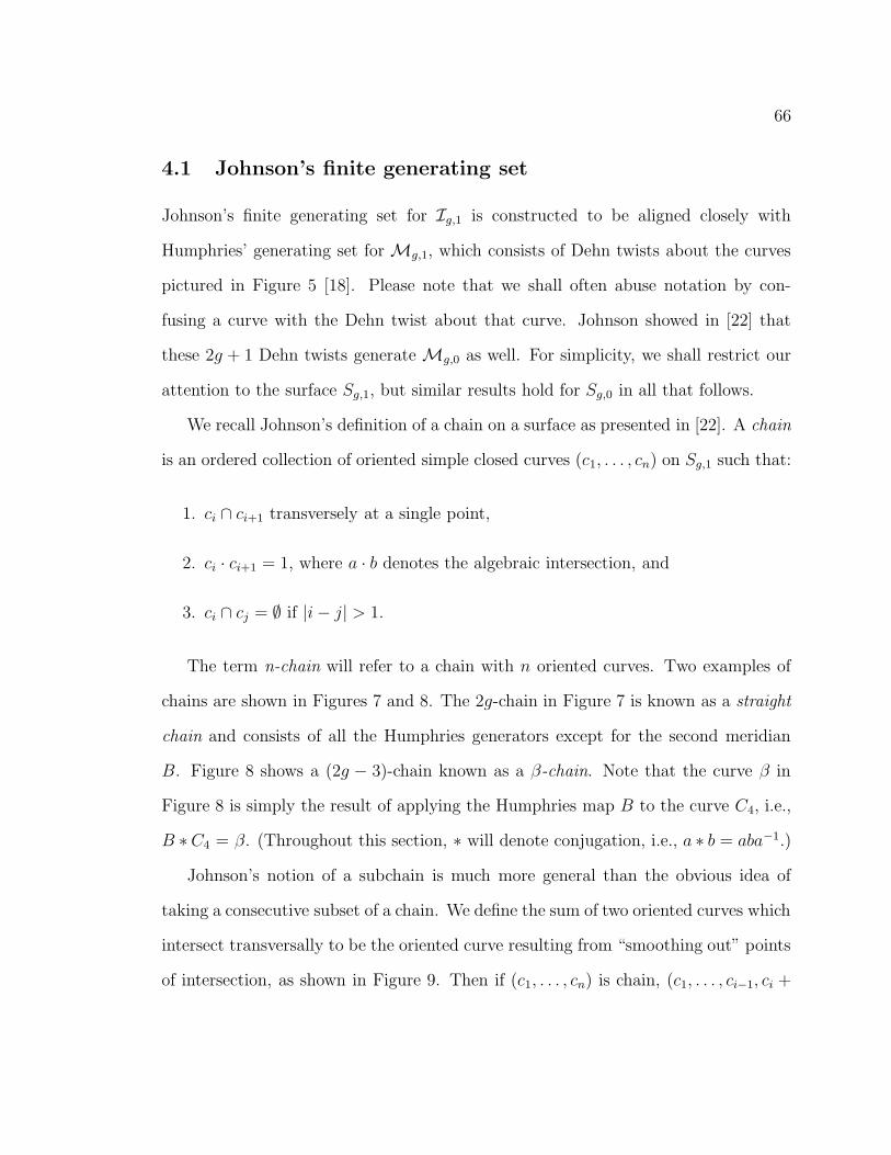
66
4.1 Johnson’s finite generating set
Johnson’s finite generating set for Ig,1 is constructed to be aligned closely with
Humphries’ generating set for Mg,1, which consists of Dehn twists about the curves
pictured in Figure 5 [18]. Please note that we shall often abuse notation by con-
fusing a curve with the Dehn twist about that curve. Johnson showed in [22] that
these 2g + 1 Dehn twists generate Mg,0 as well. For simplicity, we shall restrict our
attention to the surface Sg,1, but similar results hold for Sg,0 in all that follows.
We recall Johnson’s definition of a chain on a surface as presented in [22]. A chain
is an ordered collection of oriented simple closed curves (c1, . . . , cn) on Sg,1 such that:
1. ci ∩ ci+1 transversely at a single point,
2. ci · ci+1 = 1, where a · b denotes the algebraic intersection, and
3. ci ∩ cj = ∅ if |i− j| > 1.
The term n-chain will refer to a chain with n oriented curves. Two examples of
chains are shown in Figures 7 and 8. The 2g-chain in Figure 7 is known as a straight
chain and consists of all the Humphries generators except for the second meridian
B. Figure 8 shows a (2g − 3)-chain known as a β-chain. Note that the curve β in
Figure 8 is simply the result of applying the Humphries map B to the curve C4, i.e.,
B ∗C4 = β. (Throughout this section, ∗ will denote conjugation, i.e., a ∗ b = aba−1.)
Johnson’s notion of a subchain is much more general than the obvious idea of
taking a consecutive subset of a chain. We define the sum of two oriented curves which
intersect transversally to be the oriented curve resulting from “smoothing out” points
of intersection, as shown in Figure 9. Then if (c1, . . . , cn) is chain, (c1, . . . , ci−1, ci +

67
C1 C3 C5C2 C4 C6 C2g
Figure 7: Straight chain on Sg,1
β
C5 C6 C2g
Figure 8: β-chain on Sg,1

68
Figure 9: Summing oriented curves by smoothing out intersections
Figure 10: The straight 3-subchain (1349) on S4,1
· · ·+ cj, cj+1, . . . , cn) is also a chain. Any chain obtained from another chain after a
finite number of such summations will be called a subchain of the original chain. We
will only be concerned with straight subchains and β-subchains.
For example, (C1 + C2, C3, C4 + C5 + C6 + C7 + C8) is a straight 3-subchain map
for g ≥ 4 (see Figure 10). We shall require a shorthand notation for subchains of our
straight chains and β-chains. We use i to denote the curve Ci and β for the curve β.
A consecutive sequence of numbers (i, . . . , j) will stand for the consecutive subchain
(Ci, . . . , Cj). A gap in a sequence of numbers (i1, . . . , ij, ik, . . . , in), where ik 6= ij + 1,
will indicate the subchain (Ci1 , . . . , Cij +Cij+1 + · · ·+Cik−1, Cik , . . . , Cin). Thus, the
straight subchain given above would be denoted (1349). Note that in this example,
the curve C9 is not included in the subchain. In fact, in the case g = 4, no such curve
exists in the straight chain. In this case the number 9 merely serves as a “cut-off”,

69
Figure 11: The straight 3-subchain map [1349] on S4,1
an indication that the last curve included in the summation is C8.
In order to obtain elements of the Torelli group from these subchains, we take a
regular neighborhood K of an n-chain. If n is odd, K has two boundary components,
α and β (choose α to lie to the left of the odd-indexed curves c1, c3, . . . in the chain).
By construction, the product TαT−1β is a BP-map of genus n−1
2and hence an element
of Ig,1. We call such a map a chain map and denote it by replacing the parentheses
in the chain notation with brackets. For example, the chain map associated to the 3-
subchain given in the proceeding paragraph will be denoted [1349]. The curves which
define this BP-map are shown in Figure 11. Note that Figure 11 shows two distinct
curves. One curve is solid on the “top” of the surface and dashed when it travels
underneath the surface. The second curve is dashed with one dot on the top and
dashed with three dots underneath. The reader should take a moment to convince
himself or herself that these two curves are disjoint (or at least are isotopic to disjoint
curves), though they appear to cross when simultaneously traveling into a hole.
We are now able to state Johnson’s result.
Theorem 4.1 (Johnson, [22]) The odd straight-subchain maps together with the
odd β-chain maps generate Ig,1 and Ig,0 for g ≥ 3.

70
︸ ︷︷ ︸
k
Figure 12: The curves defining Wk.
Remark 4.2 The order of Johnson’s generating set is exponential in g. More pre-
cisely, there are 9 · 22g−3 − 4g2 + 4g − 5 Johnson generators for Ig,1 and 9 · 22g−3 −
4g2 + 2g− 6 for Ig,0. Johnson previously obtained a lower bounds of 13(4g3 + 5g + 3)
and 13(4g3 − g) for the number of generators for Ig,1 and Ig,0, respectively [21].
There is one particularly important type of Johnson generator which will appear
so often that we introduce some special notation for it. We therefore let Wk denote
the consecutive straight (2k− 1)-subchain map [234 · · · (2k+1)]. The curves defining
Wk are shown in Figure 12. We note that Wg is clearly in the kernel of the natural
map Ig,1 → Ig,0 obtained by gluing in a disk along the boundary component of Sg,1.
4.2 Lantern relations in the Torelli group
Johnson discovered relations amongst elements of the Torelli group. The main tool
he used to construct such relations is commonly known as the lantern relation in
the mapping class group. This relation was first discovered by Dehn in [11] and
independently described by Johnson in [22]. The relation is carried by the surface

71
c
a b
δ2 δ3
δ1
δ4
Figure 13: The lantern relation on S0,4
S0,4, and for the curves a, b, c, δ1, δ2, δ3, and δ4 as shown in Figure 13, we have the
following relation amongst the corresponding Dehn twists:
TcTbTa = Tδ1Tδ2Tδ3Tδ4
Clearly the left-hand side of the equation can be cyclically permuted. Also note
that for i = 1, . . . , 4, Tδicommutes with Tγ for all other curves γ in the relation since
the δi are disjoint from all other curves.
4.2.1 Johnson’s B-relations
Johnson realized that he could exploit the symmetry of certain chain maps in order to
get relations in the Torelli group out of lantern relations in the mapping class group.
We give a simple example of his method before stating the families of relations he

72
ab c
C2 C4 C6
δ
Figure 14: A lantern relation on S3,1
found in Ig,1.
Referring to Figure 14, we see that the curves in bold, C2, C4, C6 and δ, together
bound an S0,4. Thus the curves a, b, and c complete the lantern relation, and (con-
tinuing our abuse of notation in the case of the Ci), we obtain:
TcTbTa = C2C4C6Tδ. (13)
On the “bottom” of this surface, we will have another such relation. Let µ be reflection
through the plane of the page, and let γ ′ denote µ(γ). After inverting each side of
the relation, our “reflected” lantern relation becomes:
T−1c′ T
−1b′ T
−1a′ = C−1
2 C−14 C−1
6 T−1δ′ . (14)
We now combine Equations 13 and 14, noting that Dehn twists about disjoint curves
commute, to obtain:
TcT−1c′ TbT
−1b′ TaT
−1a′ = TδT
−1δ′ .

73
To simplify notation, we let Aγ denote the product TγT−1γ′ . Thus we can rewrite
our equation as follows:
AcAbAa = Aδ.
We observe that three of the four BP-maps in this relation are straight 3-subchain
maps (the reader is referred to Appendix A for a complete list of Johnsons’s generators
for genus 3). Thus we can further rewrite our equations:
Ac[4567][2345] = [234567]
Ac[4567]W2 = W3 (15)
Now, Ac is certainly a BP-map, and hence we have obtained a relation in the
Torelli group. However, Ac is not a Johnson generator, and hence we would like to
eliminate it somehow. Johnson’s method for dealing with this issue is to conjugate
Equation 15 above by B, the Dehn twist corresponding to the second meridian of the
Humphries generating set forMg,1. After doing so, we obtain:
Ac[β567]B ∗W2 = B ∗W3.
Since B commutes with Ac, we can invert Equation 15 and combine with the above
to obtain:
W−12 [4567]−1[β567]B ∗W2 = B ∗W3.
In this way, starting with the S0,4 shown in Figure 15, Johnson obtains the fol-
lowing family of relations for g ≥ 3 [22]:
W−12 [45 · · · (2g + 1)]−1[β5 · · · (2g + 1)]B ∗W2 = [23 · · · (2g + 1)]−1B ∗ [23 · · · (2g + 1)].
(16)

74
Figure 15: An S0,4 on Sg,1
As it stands, this relation is key to Johnson’s proof that his finite set of odd
subchain maps generates Ig,1. Moreover, we observe that by a lemma of Johnson
[22], B ∗W2 is a product of straight 3-subchains in I2,1. In addition, Wg lies in the
kernel of the natural map Ig,1 → Ig,0. Therefore if we pass to Ig,0, we have successfully
obtained a relation amongst Johnson generators:
W−12 [45 · · · (2g + 1)]−1[β5 · · · (2g + 1)]B ∗W2 = 1. (17)
Though this relation is not explicitly given in terms of Johnson generators, Johnson
points out that it allows us to eliminate the β-subchain map [β5 · · · (2g + 1)] in Ig,0.
In I3,0, this actually eliminates the only β-chain generator, leaving us with 35 straight
3-subchain generators and thus attaining the known lower bound on generators of Ig,0
(see Appendix A). Relation 16 also enables us to find a minimal generating set for
Ig,1, using a different argument again due to Johnson, which we will present in the
proof of Corollary 4.4 in the next section.

75
α β γ
δ1 δ2
ε
Figure 16: Another S0,4 on Sg,1
4.2.2 Generalized B-relations
Despite its usefulness in realizing a minimal generating set for genus 3, Relation 16 is
unsatisfactory on two counts. First, we do not know how to write B ∗W2 explicitly as
a product of Johnson generators, and secondly, we still do not have relations strictly
amongst Johnson generators in Ig,1. We shall now generalize Johnson’s construction
in such a way that addresses these two issues. We will do so first by generalizing
Johnson’s “B-relations”, so called because of their dependence on the second meridian
B.
The obvious generalization is to let the second “inside” boundary component of
the S0,4 contain as much genus as we like, as Johnson does with the third “inside”
boundary component to obtain his Relation 16. In other words, we begin with the
S0,4 outlined in bold in Figure 16. To keep the pictures simple, we will not draw the
image of the curves under reflection in the plane of the page, but these curves are to
be understood when required.
Remark 4.3 Note that for such an S0,4 the left-most “inside” boundary component

76
of the S0,4 must necessarily be the curve C2 as in Figure 16, since otherwise our
lantern curves will intersect the meridian B and the conjugation trick will not work.
We begin, as above, by writing down the two lantern relations corresponding to
the curves in Figure 16 to obtain:
AγAβAα = Aδ1Aδ2Aε. (18)
We assume that the curve δ1 encloses k′ holes and that the curve δ2 encloses at least
one hole. The BP-map Aγ is the only one in the relation which is not a Johnson
generator, and γ is disjoint from the curve B. Thus we are in a position to apply
the B-trick described in Section 4.2.1, and after conjugating Equation 18 by B, we
obtain:
Aγ(B ∗ Aβ)(B ∗ Aα) = (B ∗ Aδ1)Aδ2(B ∗ Aε).
Inverting Equation 18 and combining with the above yields:
A−1α A−1
β (B ∗ Aβ)(B ∗ Aα) = A−1ε A−1
δ1(B ∗Aδ1)(B ∗ Aε)
since Aδ2 commutes with everything.
We can now make the following substitutions:
Aα = Wk′+1 = [23 · · · (2k′ + 3)]
Aβ = [45 · · · (2g + 1)]
Aδ1 = [45 · · · (2k′ + 3)]
Aε = Wg = [23 · · · (2g + 1)].

77
For 1 ≤ k′ ≤ g − 2, we thus have in Ig,1:
W−1k′+1[45 · · · (2g + 1)]−1[β5 · · · (2g + 1)](B ∗Wk′+1)
= W−1g [45 · · · (2k′ + 3)]−1[β5 · · · (2k′ + 3)](B ∗Wg). (19)
In Ig,0, Wg drops out, leaving a somewhat simpler relation:
W−1k′+1[45 · · · (2g+1)]−1[β5 · · · (2g+1)](B ∗Wk′+1) = [45 · · · (2k′+3)]−1[β5 · · · (2k′+3)]
To simplify the notation a bit, we let k = k′+1. We also let Pn denote the product
[45 · · · (2n + 1)]−1[β5 · · · (2n + 1)]. We can also understand Pn as the commutator
[[45 · · · (2n+1)], B−1], where [a, b] = a−1b−1ab. Note, however, that since B /∈ Ig,1, Pn
lies in the commutator subgroup of the full mapping class group, but not necessarily
in the commutator subgroup of Ig,1. Our relation in Ig,1 now becomes:
W−1k Pg(B ∗Wk) = W−1
g Pk(B ∗Wg).
We shall refer to this relation as Rel(g, k), with 2 ≤ k ≤ g − 1.
Corollary 4.4 The Johnson generators [12 · · · (2q)] can be eliminated for 3 ≤ q ≤ g
Proof. The proof follows Johnson’s argument for eliminating the map [123456] from
the generating set of I3,1 given in Section 5 of [22]. According to Lemma 5 of [22],
the straight (2q − 1)-chain map [12 · · · (2q)] can be written as a product of B ∗Wq
and other straight (2q−1)-chain maps in Iq,1. But Rel(q, 2) allows us to write B ∗Wq
in terms of other Johnson generators. Since Iq,1 embeds in Iq+1,1 (see the proof of
Claim 2.4 in Section 2.3), we can therefore eliminate the generator [12 · · · (2q)] for all
3 ≥ q ≥ g.

78
A useful rewriting of Rel(g, k) is the following:
B ∗Wg = P−1k WgW
−1k Pg(B ∗Wk).
In Rel(g, k), everything is a Johnson generator or a product of Johnson generators
with the exception of B∗Wg and B∗Wk. In order to obtain relations strictly amongst
Johnson generators, we again make use of the fact that Ig,1 embeds in Ig+1,1. If we
let k = 2 in Rel(g, k), two nice things happen. First of all, the relation simplifies since
P2 = 1. Secondly, as previously mentioned, B ∗W2 is some product of straight 3-
subchain maps in I2,1, and so we shall at least obtain some relation amongst Johnson
generators, if not an explicit one. We therefore eliminate B ∗Wg using Rel(g, 2):
B ∗Wg = WgW−12 Pg(B ∗W2).
Similarly, we can eliminate B ∗Wk using Rel(k, 2):
B ∗Wk = WkW−12 Pk(B ∗W2).
Note that in using Rel(k, 2) we are implicitly assuming that 2 ≤ k−1 and hence that
3 ≤ k ≤ g − 1. We now substitute Rel(k, 2) and Rel(g, 2) into Rel(g, k) to obtain:
W−1k PgWkW
−12 Pk(B ∗W2) = W−1
g PkWgW−12 Pg(B ∗W2).
This is now a relation amongst Johnson generators only, but even better, B∗W2 drops
out of the relation to give the following explicit relation amongst Johnson generators:
W−1k PgWkW
−12 Pk = W−1
g PkWgW−12 Pg.
If we now multiply on the right by the map W2, we can rewrite this relation in an
interesting form.

79
Generalized B-Relation I In Ig,1, for g ≥ 4 and for 3 ≤ k ≤ g − 1, we have
(W−1k ∗ Pg)(W
−12 ∗ Pk) = (W−1
g ∗ Pk)(W−12 ∗ Pg).
There are precisely
(g − 2
2
)
such relations in Ig,1 (all relations in Ig,1 are also
relations in Ig+1,1). We note that the first generalized B-Relation can also be under-
stood as a commutator relation inMg,1:
[B−1, [45 · · · (2k + 1)]WgW−1k [45 · · · (2g + 1)]] = 1.
We obtained the first generalized B-relation by setting k = 2, a value chosen only
for the relative simplicity of Rel(g, 2). We now investigate other possible choices. Let
us begin again with Rel(g, k), 2 ≤ k ≤ g − 1. Now let us choose any l such that
2 ≤ l ≤ k − 1 (and thus k ≤ 3 and g ≤ 4). Then we can use Rel(k, l):
B ∗Wk = P−1l WkW
−1l Pk(B ∗Wl).
and also Rel(g, l):
B ∗Wg = P−1l WgW
−1l Pg(B ∗Wl).
Substituting these back into Rel(g, k), and rewriting as with the first relation, we can
now state the most general possible form of the B-relations.
Generalized B-Relation II In Ig,1, for g ≥ 4 and for 2 ≤ l < k ≤ g− 1, we have
[W−1k ∗ (PgP
−1l )][W−1
l ∗ Pk] = [W−1g ∗ (PkP
−1l )][W−1
l ∗ Pg].
Note that the second generalized B-relation contains the first in the case l = 1 (recall
P2 = 1). There are
(g − 1
3
)
such relations in Ig,1.

80
We observe that these relations involve only consecutive subchain maps, which
represent a rather small portion of the Johnson generating set. Despite this, the
relations are of value in that they currently represent the only known relations in the
Torelli group other than commutativity arising from sets of pairwise disjoint curves.
Moreover, the following lemma of Dennis Johnson allows us to see that we may use
a single relation amongst consecutive subchain maps as the basis for obtaining many
more relations amongst other non-consecutive generators.
Lemma 4.5 (Johnson, [22])
(i) Cj commutes with the subchain map [i1i2 · · · in] if and only if both j, j + 1 ∈
i1, i2, . . . , in or both j, j + 1 /∈ i1, i2, . . . , in.
(ii) If j = im, but j + 1 6= im+1, then
C−1j ∗ [i1 · · · j im+1 · · · in] = [i1 · · · (j + 1) im+1 · · · in].
(iii) If j + 1 = im, but j 6= im−1, then
Cj ∗ [i1 · · · im−1 (j + 1) · · · in] = [i1 · · · im−1 j · · · in].
The intricate notation required in the statement of the lemma unfortunately ob-
scures a simple idea which is best understood with some examples corresponding to
the three statements in the lemma:
(i) C3 commutes with the map [2345] since both 3 and 4 appear as indices in the
map. C3 also commutes with [6789] since neither 3 nor 4 appear. However, C3
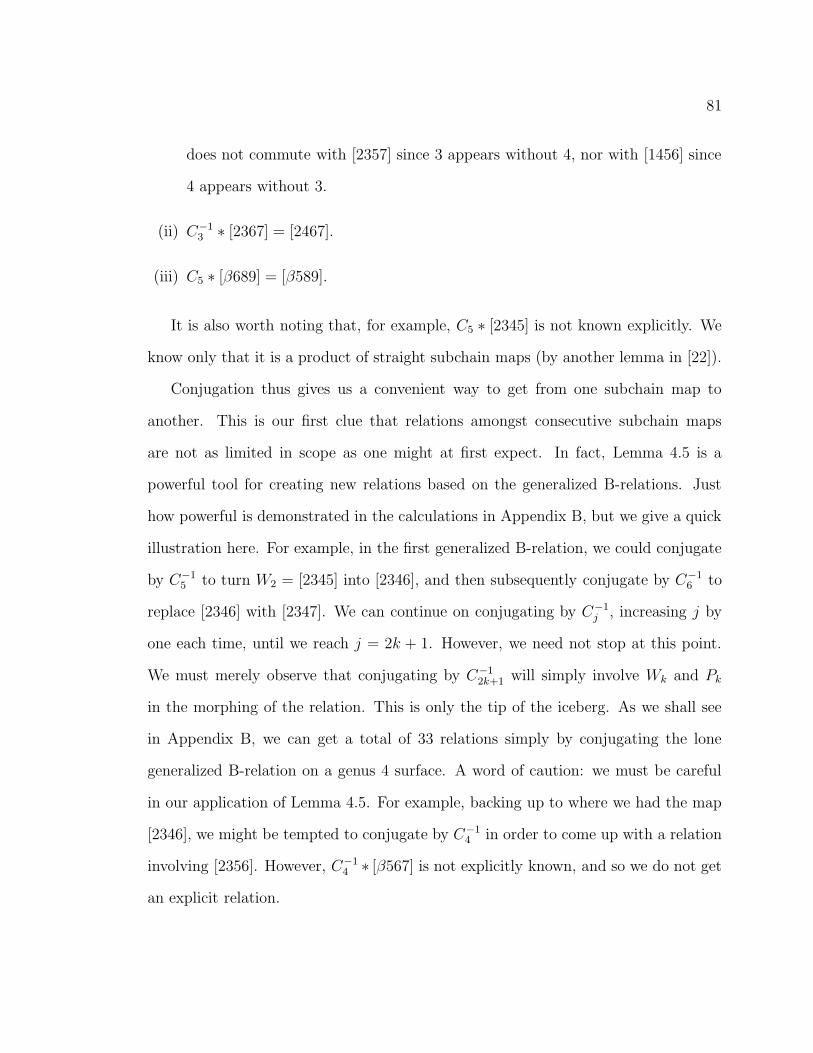
81
does not commute with [2357] since 3 appears without 4, nor with [1456] since
4 appears without 3.
(ii) C−13 ∗ [2367] = [2467].
(iii) C5 ∗ [β689] = [β589].
It is also worth noting that, for example, C5 ∗ [2345] is not known explicitly. We
know only that it is a product of straight subchain maps (by another lemma in [22]).
Conjugation thus gives us a convenient way to get from one subchain map to
another. This is our first clue that relations amongst consecutive subchain maps
are not as limited in scope as one might at first expect. In fact, Lemma 4.5 is a
powerful tool for creating new relations based on the generalized B-relations. Just
how powerful is demonstrated in the calculations in Appendix B, but we give a quick
illustration here. For example, in the first generalized B-relation, we could conjugate
by C−15 to turn W2 = [2345] into [2346], and then subsequently conjugate by C−1
6 to
replace [2346] with [2347]. We can continue on conjugating by C−1j , increasing j by
one each time, until we reach j = 2k + 1. However, we need not stop at this point.
We must merely observe that conjugating by C−12k+1 will simply involve Wk and Pk
in the morphing of the relation. This is only the tip of the iceberg. As we shall see
in Appendix B, we can get a total of 33 relations simply by conjugating the lone
generalized B-relation on a genus 4 surface. A word of caution: we must be careful
in our application of Lemma 4.5. For example, backing up to where we had the map
[2346], we might be tempted to conjugate by C−14 in order to come up with a relation
involving [2356]. However, C−14 ∗ [β567] is not explicitly known, and so we do not get
an explicit relation.

82
Counting the number of new relations we can obtain in Ig,1 from the generalized
B-relations in this way is possible, but we will skip over such a tedious computation.
It is only important to realize that each generalized B-relation stands for many, many
other relations.
4.2.3 Commutator relations
The B-relations are limited by the fact that a BP-map appearing in the initial lantern
relation which is not a Johnson generator must satisfy the condition that each of its
two defining curves be disjoint from the second meridian B. This is an extremely
restrictive condition, and so we next develop a technique whereby we are freed from
our dependence on positioning relative to the meridian B.
The basic idea is to start with a slightly different S0,4 on the surface and write
down the lantern relation. Any curve in the lantern relation which does not become
a Johnson generator when paired with its reflection in the plane of the page must
somehow be eliminated. For each such curve, we then seek another S0,4 in which the
curve plays a different role in the lantern relation, hoping to use it to eliminate these
“bad” BP-maps and obtain an explicit relation strictly amongst Johnson generators.
We begin with the S0,4 on a surface of genus 4 bounded by the curves C4, C6, δ,
and ε as shown in Figure 17. In Figures 18 - 21, the curve ε will be understood though
it is not explicitly drawn. Figure 18 illustrates the curves for a lantern relation on
this S0,4. As usual, we reflect through the plane of the page, invert the resulting
relation, and combine the two to obtain a relation amongst BP-maps. For curves
which are not Johnson generators, we continue the notation of the previous section.
For simplicity in the notation of later relations, we will use a different notation system
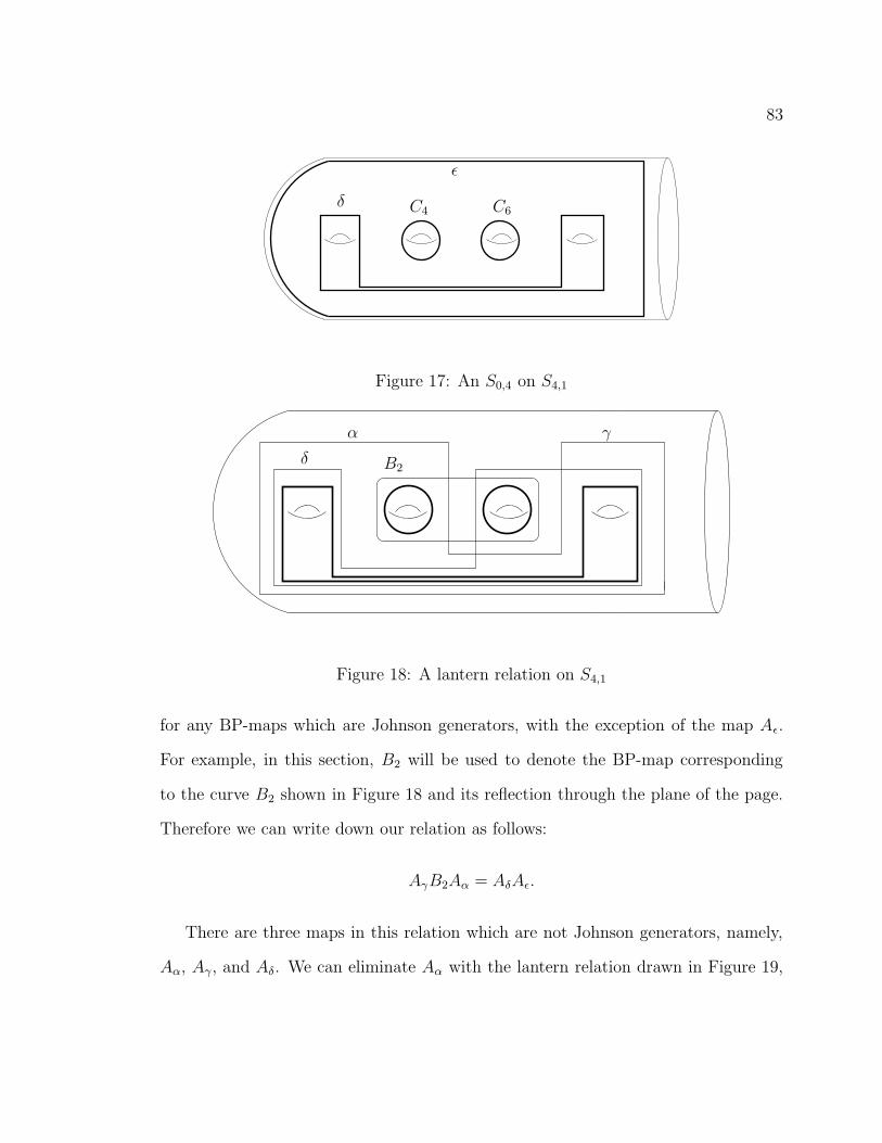
83
C4 C6δ
ε
Figure 17: An S0,4 on S4,1
B2
γ
δ
α
Figure 18: A lantern relation on S4,1
for any BP-maps which are Johnson generators, with the exception of the map Aε.
For example, in this section, B2 will be used to denote the BP-map corresponding
to the curve B2 shown in Figure 18 and its reflection through the plane of the page.
Therefore we can write down our relation as follows:
AγB2Aα = AδAε.
There are three maps in this relation which are not Johnson generators, namely,
Aα, Aγ, and Aδ. We can eliminate Aα with the lantern relation drawn in Figure 19,

84
B1
B3A1
α
Figure 19: Eliminating Aα
A2
γ
B1
B3
Figure 20: Eliminating Aγ
which yields the following BP-relation:
A1B3Aα = B1Aε
or solving for Aα:
Aα = B−13 A−1
1 B1Aε.
Similarly, we can eliminate Aγ and Aδ by using the lantern relations given in

85
B2
A2
A1
δ
Figure 21: Eliminating Aδ
Figures 20 and 21, respectively. We get the following relations:
Aγ = B3AεB−11 A−1
2
Aδ = B2AεA−11 A−1
2 .
Substituting in for Aα, Aγ, and Aδ, we see that Aε drops out of the relation (the curve
ε is disjoint from all other curves involved in the relation). The result is:
B3B−11 A−1
2 B2B−13 A−1
1 B1 = B2A−11 A−1
2 .
This relation looks a bit unwieldy at first, but after some reorganizing using the
fact that many pairs of these BP-maps commute, we realize that it is actually a
commutativity relation:
(B−11 A1B3)(A2B
−12 ) = (A2B
−12 )(B−1
1 A1B3).
or
[(B−11 A1B3), (A2B
−12 )] = 1. (20)

86
B1
A1
B3
Figure 22: Curves defining the product B−11 A1B3
The curves involved within each of the two products in the commutator relation are
given in Figures 22 and 23, respectively. It is also interesting to rewrite Relation 20
as a “not quite commuting” relation:
(A2B−12 )(A1B
−11 ) = (A1B
−11 )[B3 ∗ (A2B
−12 )].
It is worth noting that this relation cannot be obtained merely by a straightforward
applicatoin of the commutativity relations between the various pairs of Johnson gen-
erators.
This single elementary idea gives us a wealth of relations amongst Johnson gener-
ators. To begin with, we can simply turn the picture upside down to obtain another
commutator relation:
[A1B−12 , A2B1B
−13 ] = 1.
We can also rewrite the relation using Johnson’s notation. We have:
A1 = [234567] = W3
A2 = [456789]

87
A2
B2
Figure 23: Curves defining the product A2B−12
εδ J2 J3
Figure 24: An S0,4 on a higher genus surface
B1 = [2345] = W2
B2 = [4567]
B3 = [6789]
Lemma 4.5 can also be applied to this commutativity relations to obtain new
commutativity relations amongst certain non-consecutive straight subchain maps.
Furthermore, we can find analogous relations in higher genus by applying the same
idea to the S0,4 shown in Figure 24.
If we define analogous curves α and γ, and introduce the curves J1 and J4 as

88
α γ
J2 J3J1 J4
Figure 25: Lantern curves
shown in Figure 25, we can write down the following relation:
AγB2Aα = AδAεJ2J3
Now we simply find three new lantern relations analogous to those given in Fig-
ures 19, 20, and 21. The only difference is that now we have the curves Ji in our
relations. We find that we can make the following substitutions:
Aα = B−13 A−1
1 B1AεJ3J4
Aγ = B3AεB−11 A−1
2 J1J2
Aδ = B2AεA−11 A−1
2 J1J4
Noting that Aε and the Ji commute with every map in these lantern relations, we
see that these factors drop out of the relation, and we are left with the precise analog
of our genus 4 commutator relation:
General Commutator Relation In Ig,1, for g ≥ 4 and for the curves shown in
Figure 26, we have
[(B−11 A1B3), (A2B
−12 )] = 1.

89
A1A2
B1B2 B3
Figure 26: Curves in the generalized commutator relation
We need some notation at this point, so we assume that Bi encloses the mthi hole
to the (mi+2 − 1)th hole. In other words, Bi “begins” with the mthi hole and ends
before the mthi+2 hole. Thus our curves represent the following Johnson generators:
A1 = [(2m1)(2m1 + 1) · · · (2m4)]
A2 = [(2m2)(2m2 + 1) · · · (2m5)]
B1 = [(2m1)(2m1 + 1) · · · (2m3)]
B2 = [(2m2)(2m1 + 1) · · · (2m4)]
B3 = [(2m3)(2m1 + 1) · · · (2m5)]
We can of course use Lemma 4.5 on all these relations to obtain morelations.
Remark 4.6 Johnson found other lantern relations amongst elements of Ig,1. For
example, also in [22], he finds that
[1234][1256 · · ·2g](B ∗ [345 · · ·2g]) = [56 · · ·2g][123 · · ·2g].
This relation is not useful for our present purpose since B ∗ [345 · · ·2g] is not a
Johnson generator. All efforts to use either of our two methods introduced are in

90
vain, however. We have no recursively defined relation with which to take advantage
of the embeddings of Ig,1 in higher genus groups, as in Section 4.2.2. After some
calculations, one also finds that when attempting to apply the technique of letting
“bad” curves play different roles in other lantern relations as in Section 4.2.3, one
simply runs out of room on the surface. Thus the real trick to finding relations
amongst Johnson generators is to find a “good” S0,4 in the first place.
4.3 Symmetry of straight chain maps and further questions
There is a great deal of interesting geometry in the Johnson generating set. As one
might guess from the symmetry of the straight chain itself, it turns out that each
straight subchain map TαT−1β has the property that rotation through 180 degrees
about the axis shown in Figure 27 takes the curve α onto β (see, for instance, the
straight 3-subchain given in Figure 11). Let us call this rotation j. The centralizer
of j in Mg,b,n is known as the hyperelliptic subgroup of Mg,b,n and is known to be
linear ([3], [29]). Now, let A denote a Johnson generator TαT−1β . It is not true that
A commutes with j; however we do have the property that jAj−1 = A−1. It also
has the immediate consequence that the product jA is itself an involution and also
that A = [T−1α , j]. This is an intriguing property in its own right, and, since Johnson
shows in [22] that I3,0 is generated by 35 straight 3-subchain maps (given explicitly in
Appendix A), it piques one’s curiosity regarding the linearity question for the Torelli
group in genus 3. One also could hope to generalize any result along these lines to
higher genus to a certain extent, since the vast majority of Johnson generators are
straight subchain maps.
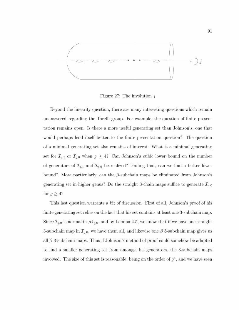
91
j
Figure 27: The involution j
Beyond the linearity question, there are many interesting questions which remain
unanswered regarding the Torelli group. For example, the question of finite presen-
tation remains open. Is there a more useful generating set than Johnson’s, one that
would perhaps lend itself better to the finite presentation question? The question
of a minimal generating set also remains of interest. What is a minimal generating
set for Ig,1 or Ig,0 when g ≥ 4? Can Johnson’s cubic lower bound on the number
of generators of Ig,1 and Ig,0 be realized? Failing that, can we find a better lower
bound? More particularly, can the β-subchain maps be eliminated from Johnson’s
generating set in higher genus? Do the straight 3-chain maps suffice to generate Ig,0
for g ≥ 4?
This last question warrants a bit of discussion. First of all, Johnson’s proof of his
finite generating set relies on the fact that his set contains at least one 3-subchain map.
Since Ig,0 is normal inMg,0, and by Lemma 4.5, we know that if we have one straight
3-subchain map in Ig,0, we have them all, and likewise one β 3-subchain map gives us
all β 3-subchain maps. Thus if Johnson’s method of proof could somehow be adapted
to find a smaller generating set from amongst his generators, the 3-subchain maps
involved. The size of this set is reasonable, being on the order of g4, and we have seen

92
that straight 3-chain maps suffice to generate I3,0. This bit of speculation of course
leads to another question: is there a generating set better suited than Johnson’s to
attaining a minimal set?
Furthermore, we might ask what the intersection of the Torelli group is with other
interesting subgroups of the mapping class group, such as the handlebody subgroup,
or the Crisp-Paris subgroups [10], which are right-angled Artin groups (and hence
linear) generated by squares of certain Dehn twists? As discussed in Section 3, the
former question arises in the context of classifying Heegaard splittings of 3-manifolds,
yet another context in which better knowledge of the Torelli group could have vast
implications.
These and many other questions must be answered if enormous potential of the
Torelli group is to be realized fully.

93
A Johnson’s generators in genus 3
We present here a complete and explicit list of all Johnson’s generators for both I3,1
and I3,0, with a summary of relevant facts from Section 4.
1. In the genus 3 case, Johnson’s generators are all straight subchain maps with
the exception of a single β-subchain map.
2. We first give the 5-subchain maps (six indices), followed by the 3-subchain maps
(four indices).
3. The straight 5-subchain maps listed all lie in the kernel of the natural map
Ig,1 → Ig,0.
4. Since all straight subchain maps have rotational symmetry, as discussed in Sec-
tion 4.3, for such maps we only give one of the two curves defining the BP-map.
The second can then be obtained by applying the involution j shown in Fig-
ure 27.
5. In the case of the β-subchain, both curves are drawn.
6. The 36 3-subchain maps together with all of the 5-subchain maps but the first
([123456]) represent a minimal generating set for I3,1.
7. The 35 straight 3-subchain maps (which have four indices) shown here represent
a minimal generating set for I3,0.
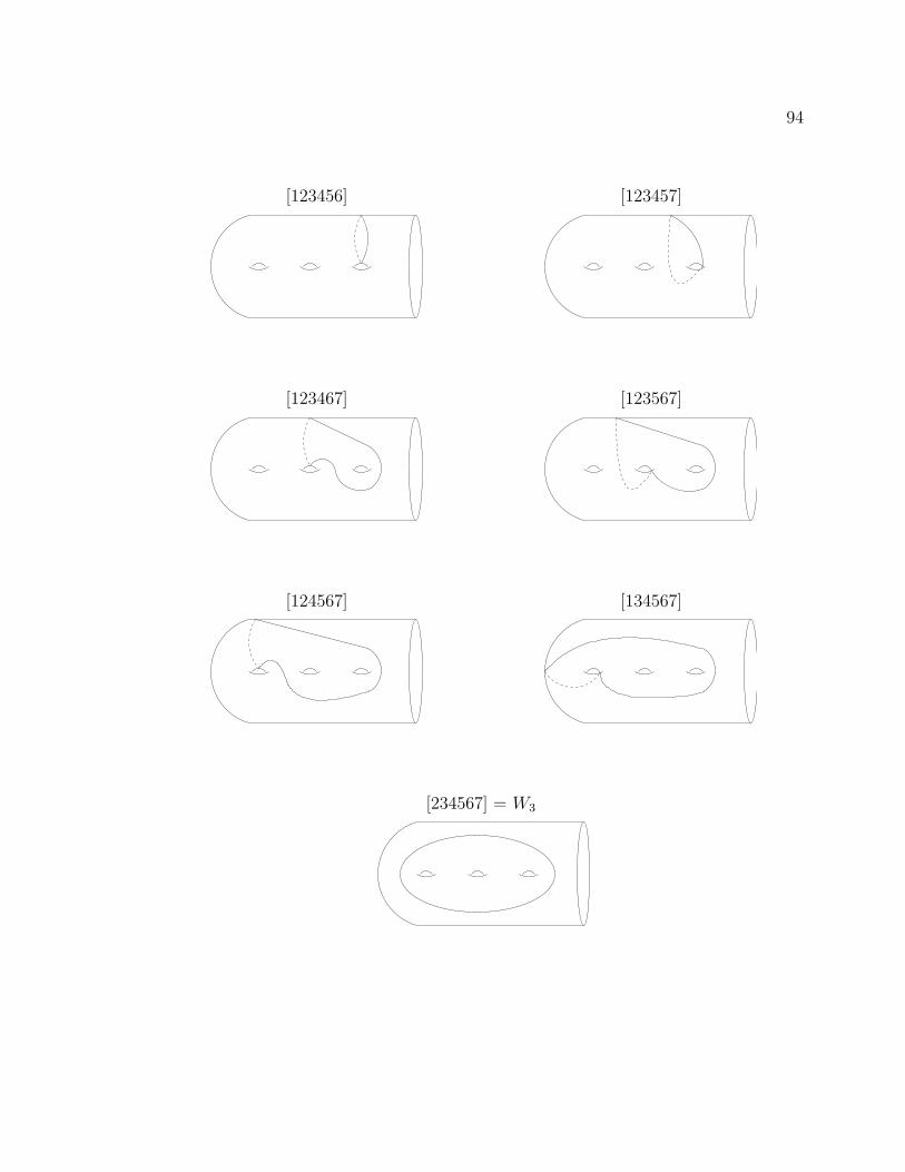
94
[123456] [123457]
[123467] [123567]
[124567] [134567]
[234567] = W3

95
[1234] [1235]
[1236] [1237]
[1245] [1246]
[1247] [1256]

96
[1257] [1267]
[1345] [1346]
[1347] [1356]
[1357] [1367]

97
[1456] [1457]
[1467] [1567]
[2345] = W2 [2346]
[2347] [2356]

98
[2357] [2367]
[2456] [2457]
[2467] [2567]
[3456] [3457]

99
[3467] [3567]
[4567] [β 567]

100
B Some calculations of relations in low genus
Before getting started with calculations in genus 4, we note that Johnson’s Equa-
tion 16 gives us a single relation in I3,0, though it is not explicit since we only know
that B ∗W2 is a product of straight 3-chains in I2, 1. The relation is as follows:
W−12 [4567]−1[β567]B ∗W2 = 1.
Since mapping class groups of closed surfaces do not embed in higher genus mapping
class groups, this does not give us an explicit form for B∗W2. As previously discussed
in Section 4.2.1, it does allow us to eliminate the generator [β567] from Johnson’s
generating set in I3,0. Note that we could rewrite the above relation in the notation
of Section 4 as follows:
W−12 P3B ∗W2 = 1
or equivalently,
P3 = [W2, B−1]
We also have the analogous relation in Ig,0:
Pg = [W ,2B ∗W2].
Turning now to the surface with one boundary component, we calculate all rela-
tions arising from the generalized B-relation in the simplest case, I4,1.
There is only one generalized B-relation in genus 4, with k = 3 (and l = 2):
(W−13 ∗ P4)(W
−12 ∗ P3) = (W−1
4 ∗ P3)(W−12 ∗ P4)
. We write this out in Johnson’s notation so that we can find all conjugates:
[234567]−1 ∗ ([456789]−1[β56789]) · [2345]−1 ∗ ([4567]−1[β567])
= [23456789]−1 ∗ ([4567]−1[β567]) · [2345]−1 ∗ ([456789]−1[β56789]) (1)

101
Conjugate by C−15 and then by C−1
6 to obtain the next two relations:
[234567]−1 ∗ ([456789]−1[β56789]) · [2346]−1 ∗ ([4567]−1[β567])
= [23456789]−1 ∗ ([4567]−1[β567]) · [2346]−1 ∗ ([456789]−1[β56789]) (2)
[234567]−1 ∗ ([456789]−1[β56789]) · [2347]−1 ∗ ([4567]−1[β567])
= [23456789]−1 ∗ ([4567]−1[β567]) · [2347]−1 ∗ ([456789]−1[β56789]) (3)
Now conjugate by C−17 , which involves four more factors, with result:
[234568]−1 ∗ ([456789]−1[β56789]) · [2348]−1 ∗ ([4568]−1[β568])
= [23456789]−1 ∗ ([4568]−1[β568]) · [2348]−1 ∗ ([456789]−1[β56789]) (4)
Then conjugate by C−18 :
[234569]−1 ∗ ([456789]−1[β56789]) · [2349]−1 ∗ [4569]−1[β569])
= [23456789]−1 ∗ ([4569]−1[β569]) · [2349]−1 ∗ ([456789]−1[β56789]) (5)
Note that the genus 4 relations embed in all higher genus, and in that case, we could
continue on in this way until running out of genus.
We now work on the “middle” of the indices. Beginning with Relation 4 we have
some room to maneuver inside the larger factors. First we conjugate Relation 4 by
C−16 and then by C−1
5 :
[234578]−1 ∗ ([456789]−1[β56789]) · [2348]−1 ∗ ([4578]−1[β578])
= [23456789]−1 ∗ ([4578]−1[β578]) · [2348]−1 ∗ ([456789]−1[β56789]) (6)

102
[234678]−1 ∗ ([456789]−1[β56789]) · [2348]−1 ∗ ([4678]−1[β678])
= [23456789]−1 ∗ ([4678]−1[β678]) · [2348]−1 ∗ ([456789]−1[β56789]) (7)
We can create even more relations from Relation 5 by conjugating by C−16 , C−1
7 , C−15 ,
and C−16 (in that order) to obtain, the following four relations, respectively:
[234579]−1 ∗ ([456789]−1[β56789]) · [2349]−1 ∗ ([4579]−1[β579])
= ([23456789]−1 ∗ [4579]−1[β579])([2349]−1 ∗ [456789]−1[β56789]) (8)
[234589]−1 ∗ ([456789]−1[β56789]) · [2349]−1 ∗ ([4589]−1[β589])
= [23456789]−1 ∗ ([4589]−1[β589]) · [2349]−1 ∗ ([456789]−1[β56789]) (9)
[234689]−1 ∗ ([456789]−1[β56789]) · [2349]−1 ∗ ([4689]−1[β689])
= [23456789]−1 ∗ ([4689]−1[β689]) · [2349]−1 ∗ ([456789]−1[β56789]) (10)
[234789]−1 ∗ ([456789]−1[β56789]) · [2349]−1 ∗ ([4789]−1[β789])
= [23456789]−1 ∗ ([4789]−1[β789]) · [2349]−1 ∗ ([456789]−1[β56789]) (11)
At this point, we are stuck on the 4’s, i.e., we cannot conjugate by C−14 to obtain,
for example, [2359] in place of [2349], since C−14 clashes with the β-subchain maps. So
we turn our attention to the lower indices. We begin again with the original relation:
[234567]−1 ∗ ([456789]−1[β56789]) · [2345]−1 ∗ ([4567]−1[β567])
= [23456789]−1 ∗ ([4567]−1[β567]) · [2345]−1 ∗ ([456789]−1[β56789])

103
We now conjugate by C1 and then by C2, which involves three factors.
[134567]−1 ∗ ([456789]−1[β56789]) · [1345]−1 ∗ ([4567]−1[β567])
= [13456789]−1 ∗ ([4567]−1[β567]) · [1345]−1 ∗ ([456789]−1[β56789]) (12)
[124567]−1 ∗ ([456789]−1[β56789]) · [1245]−1 ∗ ([4567]−1[β567])
= [12456789]−1 ∗ ([4567]−1[β567]) · [1245]−1 ∗ ([456789]−1[β56789]) (13)
We can also conjugate Relation 3 by C1 and then by C2, and then do the same
for Relation 3, to obtain four more relations:
[134567]−1 ∗ ([456789]−1[β56789]) · [1346]−1 ∗ ([4567]−1[β567])
= [13456789]−1 ∗ ([4567]−1[β567]) · [1346]−1 ∗ ([456789]−1[β56789]) (14)
[124567]−1 ∗ ([456789]−1[β56789]) · [1246]−1 ∗ ([4567]−1[β567])
= [12456789]−1 ∗ ([4567]−1[β567]) · [1246]−1 ∗ ([456789]−1[β56789]) (15)
[134567]−1 ∗ ([456789]−1[β56789]) · [1347]−1 ∗ ([4567]−1[β567])
= [13456789]−1 ∗ ([4567]−1[β567]) · [1347]−1 ∗ ([456789]−1[β56789]) (16)
[124567]−1 ∗ ([456789]−1[β56789]) · [1247]−1 ∗ ([4567]−1[β567])
= [12456789]−1 ∗ ([4567]−1[β567]) · [1247]−1 ∗ ([456789]−1[β56789]) (17)

104
We finish off the generalized B-relations by repeating this for Relations 4 - 11.
[134568]−1 ∗ ([456789]−1[β56789]) · [1348]−1 ∗ ([4568]−1[β568])
= [13456789]−1 ∗ ([4568]−1[β568]) · [1348]−1 ∗ ([456789]−1[β56789]) (18)
[124568]−1 ∗ ([456789]−1[β56789]) · [1248]−1 ∗ ([4568]−1[β568])
= [12456789]−1 ∗ ([4568]−1[β568]) · [1248]−1 ∗ ([456789]−1[β56789]) (19)
[134569]−1 ∗ ([456789]−1[β56789]) · [1349]−1 ∗ [4569]−1[β569])
= [13456789]−1 ∗ ([4569]−1[β569]) · [1349]−1 ∗ ([456789]−1[β56789]) (20)
[124569]−1 ∗ ([456789]−1[β56789]) · [1249]−1 ∗ [4569]−1[β569])
= [12456789]−1 ∗ ([4569]−1[β569]) · [1249]−1 ∗ ([456789]−1[β56789]) (21)
[134578]−1 ∗ ([456789]−1[β56789]) · [1348]−1 ∗ ([4578]−1[β578])
= [13456789]−1 ∗ ([4578]−1[β578]) · [1348]−1 ∗ ([456789]−1[β56789]) (22)
[124578]−1 ∗ ([456789]−1[β56789]) · [1248]−1 ∗ ([4578]−1[β578])
= [12456789]−1 ∗ ([4578]−1[β578]) · [1248]−1 ∗ ([456789]−1[β56789]) (23)
[134678]−1 ∗ ([456789]−1[β56789]) · [1348]−1 ∗ ([4678]−1[β678])
= [13456789]−1 ∗ ([4678]−1[β678]) · [1348]−1 ∗ ([456789]−1[β56789]) (24)

105
[124678]−1 ∗ ([456789]−1[β56789]) · [1248]−1 ∗ ([4678]−1[β678])
= [12456789]−1 ∗ ([4678]−1[β678]) · [1248]−1 ∗ ([456789]−1[β56789]) (25)
[134579]−1 ∗ ([456789]−1[β56789]) · [1349]−1 ∗ ([4579]−1[β579])
= ([13456789]−1 ∗ [4579]−1[β579])([1349]−1 ∗ [456789]−1[β56789]) (26)
[124579]−1 ∗ ([456789]−1[β56789]) · [1249]−1 ∗ ([4579]−1[β579])
= ([12456789]−1 ∗ [4579]−1[β579])([1249]−1 ∗ [456789]−1[β56789]) (27)
[134589]−1 ∗ ([456789]−1[β56789]) · [1349]−1 ∗ ([4589]−1[β589])
= [13456789]−1 ∗ ([4589]−1[β589]) · [1349]−1 ∗ ([456789]−1[β56789]) (28)
[124589]−1 ∗ ([456789]−1[β56789]) · [1249]−1 ∗ ([4589]−1[β589])
= [12456789]−1 ∗ ([4589]−1[β589]) · [1249]−1 ∗ ([456789]−1[β56789]) (29)
[134689]−1 ∗ ([456789]−1[β56789]) · [1349]−1 ∗ ([4689]−1[β689])
= [13456789]−1 ∗ ([4689]−1[β689]) · [1349]−1 ∗ ([456789]−1[β56789]) (30)
[124689]−1 ∗ ([456789]−1[β56789]) · [1249]−1 ∗ ([4689]−1[β689])
= [12456789]−1 ∗ ([4689]−1[β689]) · [1249]−1 ∗ ([456789]−1[β56789]) (31)

106
[134789]−1 ∗ ([456789]−1[β56789]) · [1349]−1 ∗ ([4789]−1[β789])
= [13456789]−1 ∗ ([4789]−1[β789]) · [1349]−1 ∗ ([456789]−1[β56789]) (32)
[124789]−1 ∗ ([456789]−1[β56789]) · [1249]−1 ∗ ([4789]−1[β789])
= [12456789]−1 ∗ ([4789]−1[β789]) · [1249]−1 ∗ ([456789]−1[β56789]) (33)
The reader who attempts to perform such a calculation in higher genus or for the
commutativity relations will quickly appreciate the desirability of using a computer
for such a task.

107
References
[1] Hyman Bass. Covering theory for graphs of groups. J. Pure Appl. Algebra,
89(1-2):3–47, 1993.
[2] Stephen J. Bigelow. Braid groups are linear. J. Amer. Math. Soc., 14(2):471–486
(electronic), 2001.
[3] Stephen J. Bigelow and Ryan D. Budney. The mapping class group of a genus
two surface is linear. Algebr. Geom. Topol., 1:699–708 (electronic), 2001.
[4] Joan S. Birman. Braids, links, and mapping class groups. Princeton University
Press, Princeton, N.J., 1974. Annals of Mathematics Studies, No. 82.
[5] Joan S. Birman. On the equivalence of Heegaard splittings of closed, orientable
3-manifolds. In Knots, groups, and 3-manifolds (Papers dedicated to the memory
of R. H. Fox), pages 137–164. Ann. of Math. Studies, No. 84. Princeton Univ.
Press, Princeton, N.J., 1975.
[6] Joan S. Birman, Alex Lubotzky, and John McCarthy. Abelian and solvable
subgroups of the mapping class groups. Duke Math. J., 50(4):1107–1120, 1983.
[7] Tara E. Brendle and Hessam Hamidi-Tehrani. On the linearity problem for
mapping class groups. Algebr. Geom. Topol., 1:445–468 (electronic), 2001.
[8] Kenneth S. Brown. Cohomology of groups. Springer-Verlag, New York, 1982.
[9] D. R. J. Chillingworth. Winding numbers on surfaces. I. Math. Ann., 196:218–
249, 1972.

108
[10] John Crisp and Luis Paris. The solution to a conjecture of Tits on the subgroup
generated by the squares of the generators of an Artin group. Invent. Math.,
145(1):19–36, 2001.
[11] Max Dehn. Die gruppe der abbildungsklassen. Acta Math., 69:113–206, 1938.
English transl.: [43], 256-362.
[12] Joan L. Dyer, Edward Formanek, and Edna K. Grossman. On the linearity of
automorphism groups of free groups. Arch. Math. (Basel), 38(5):404–409, 1982.
[13] D. B. A. Epstein. Curves on 2-manifolds and isotopies. Acta Math., 115:83–107,
1966.
[14] Edward Formanek and Claudio Procesi. The automorphism group of a free group
is not linear. J. Algebra, 149(2):494–499, 1992.
[15] Joel Hass and Peter Scott. Shortening curves on surfaces. Topology, 33(1):25–43,
1994.
[16] A. Hatcher and W. Thurston. A presentation for the mapping class group of a
closed orientable surface. Topology, 19(3):221–237, 1980.
[17] Peter John Hilton and Urs Stammbach. A course in homological algebra.
Springer-Verlag, New York, 1971. Graduate Texts in Mathematics, Vol. 4.
[18] Stephen P. Humphries. Generators for the mapping class group. In Topology of
low-dimensional manifolds (Proc. Second Sussex Conf., Chelwood Gate, 1977),
pages 44–47. Springer, Berlin, 1979.

109
[19] Nikolai V. Ivanov. Subgroups of Teichmuller modular groups. American Mathe-
matical Society, Providence, RI, 1992. Translated from the Russian by E. J. F.
Primrose and revised by the author.
[20] Dennis Johnson. An abelian quotient of the mapping class group Ig. Math. Ann.,
249(3):225–242, 1980.
[21] Dennis Johnson. Quadratic forms and the Birman-Craggs homomorphisms.
Trans. Amer. Math. Soc., 261(1):235–254, 1980.
[22] Dennis Johnson. The structure of the Torelli group. I. A finite set of generators
for I. Ann. of Math. (2), 118(3):423–442, 1983.
[23] Dennis Johnson. A survey of the Torelli group. In Low-dimensional topology
(San Francisco, Calif., 1981), pages 165–179. Amer. Math. Soc., Providence, RI,
1983.
[24] Dennis Johnson. The structure of the Torelli group. II. A characterization of the
group generated by twists on bounding curves. Topology, 24(2):113–126, 1985.
[25] Dennis Johnson. The structure of the Torelli group. III. The abelianization of
T . Topology, 24(2):127–144, 1985.
[26] Dennis L. Johnson. Homeomorphisms of a surface which act trivially on homol-
ogy. Proc. Amer. Math. Soc., 75(1):119–125, 1979.
[27] Yasushi Kasahara. An expansion of the Jones representation of genus 2 and the
Torelli group. Algebr. Geom. Topol., 1:39–55 (electronic), 2001.

110
[28] Rob Kirby. Problems in low dimensional manifold theory. In Algebraic and
geometric topology (Proc. Sympos. Pure Math., Stanford Univ., Stanford, Calif.,
1976), Part 2, pages 273–312. Amer. Math. Soc., Providence, R.I., 1978.
[29] Mustafa Korkmaz. On the linearity of certain mapping class groups. Turkish J.
Math., 24(4):367–371, 2000.
[30] Daan Krammer. The braid group B4 is linear. Invent. Math., 142(3):451–486,
2000.
[31] Catherine Labruere and Luis Paris. Presentations for the punctured mapping
class groups in terms of Artin groups. Algebr. Geom. Topol., 1:73–114 (elec-
tronic), 2001.
[32] Gilbert Levitt and Karen Vogtmann. A Whitehead algorithm for surface groups.
Topology, 39(6):1239–1251, 2000.
[33] Wilhelm Magnus, Abraham Karrass, and Donald Solitar. Combinatorial group
theory. Dover Publications Inc., New York, revised edition, 1976. Presentations
of groups in terms of generators and relations.
[34] Makoto Matsumoto. A presentation of mapping class groups in terms of Artin
groups and geometric monodromy of singularities. Math. Ann., 316(3):401–418,
2000.
[35] John McCarthy. A “Tits-alternative” for subgroups of surface mapping class
groups. Trans. Amer. Math. Soc., 291(2):583–612, 1985.

111
[36] Geoffrey Mess. The Torelli groups for genus 2 and 3 surfaces. Topology,
31(4):775–790, 1992.
[37] Shigeyuki Morita. Families of Jacobian manifolds and characteristic classes of
surface bundles. I. Ann. Inst. Fourier (Grenoble), 39(3):777–810, 1989.
[38] Shigeyuki Morita. Families of Jacobian manifolds and characteristic classes of
surface bundles. II. Math. Proc. Cambridge Philos. Soc., 105(1):79–101, 1989.
[39] Shigeyuki Morita. The extension of Johnson’s homomorphism from the Torelli
group to the mapping class group. Invent. Math., 111(1):197–224, 1993.
[40] J. Nielsen. Die gruppe der dreidimensionalen gittertransformationen. Danske
Vid. Selsk. Mat-Fys., pages 1–29, 1924.
[41] Bernard Perron. A linear representation of finite rank of the mapping class group
of surfaces (preprint). Laboratoire de Topologie, 99(204), 1999.
[42] Jerome Powell. Two theorems on the mapping class group of a surface. Proc.
Amer. Math. Soc., 68(3):347–350, 1978.
[43] Dale Rolfsen. Knots and links. Publish or Perish Inc., Houston, TX, 1990.
Corrected reprint of the 1976 original.
[44] Patricia L. Sipe. Some finite quotients of the mapping class group of a surface.
Proc. Amer. Math. Soc., 97(3):515–524, 1986.
[45] Craig C. Squier. Matrix representations of Artin groups. Proc. Amer. Math.
Soc., 103(1):49–53, 1988.

112
[46] Rolland Trapp. A linear representation of the mapping class group M and the
theory of winding numbers. Topology Appl., 43(1):47–64, 1992.
[47] Karen Vogtmann. Automorphisms of free groups and outer space. Geometriae
Dedicata, To appear in the special issue for the June, 2000 Haifa conference.
Available at http://www.math.cornell.edu/ vogtmann/papers/Autosurvey/.
[48] Bronislaw Wajnryb. A simple presentation for the mapping class group of an
orientable surface. Israel J. Math., 45(2-3):157–174, 1983.
[49] Bronislaw Wajnryb. An elementary approach to the mapping class group of a
surface. Geom. Topol., 3:405–466 (electronic), 1999.
[50] B. A. F. Wehrfritz. Infinite linear groups. An account of the group-theoretic prop-
erties of infinite groups of matrices. Springer-Verlag, New York, 1973. Ergebnisse
der Matematik und ihrer Grenzgebiete, Band 76.
[51] Gretchen Wright. The Reshetikhin-Turaev representation of the mapping class
group. J. Knot Theory Ramifications, 3(4):547–574, 1994.