THEO CHEM

Journal of Molecular Structure (Theochem) 336 (1995) 269-278

The topology of Hilbert spaces and the dynamics of molecular processes

M. Howard Leea’*, Jangil Kim”, William P. Cummings”, Raf Dekeyserb

aDepartment of Physics and Astronomy, University of Georgia, Athens, GA 30602, USA blnsrituut voor Theoretische Fysica, Kutholieke Universiteit Leuven, B-3001 Heverlee. Belgium

Received 28 September 1994; accepted 20 October 1994

Abstract

The transfer of energy from one mode to another whether within a molecule or between molecules is a fundamental process in nature. The delocalization of energy which encompasses energy transfer is closely related to time evolution in a system. The recently developed method of recurrence relations shows that the time evolution and the topology of a particular Hilbert space structure are equivalent. In this work a number of different topological shapes of infinite- dimensional Hilbert spaces obtained from microscopic models are summarized to illustrate a variety of admissible time-evolution functions.

1. Introduction

At the most basic level the dynamics of

molecular processes refers to the transfer of energy. How energy is transferred from one mode to another whether within one molecule or among molecules, or how it can become localized in a mode, is central to this subject. If a system (be it a single molecule or a collection of identical molecules) is perturbed by some external means, the signature of the delocalization of the perturba- tion energy is in the time evolution in that system. The delocalization depends on the characteristics of the perturbed system, but not on the manner in which it is perturbed if linear response theory is followed. The time evolution in this system will be reflective of some critical features of the internal structure of this system and will be distinctive. One

* Corresponding author.

may expect that there are a variety of ways different systems can evolve in time. It is of utmost interest that, for Hermitian systems, there is an admissible class of functions for the time evolution. It implies that for these systems their internal structures are not limitless in scope.

A system may be of finite size containing a finite number of particles as in an ordinary molecule or it may be of infinite size containing an infinite number of particles as in a polymer. The time evolution in a finite system will in general be very different from that in an infinite system. If there exists a localization in an infinite system, it can however resemble the time evolution in a finite system. In this work we shall consider models of both finite and infinite systems. These are models which can in many cases represent some critical properties of molecular systems. Some of them may perhaps be too simple to represent any system realistically. But they can still provide some useful

0166-1280/95/$09.50 0 1995 Elsevier Science B.V. All rights reserved SSDI 0166-1280(94)04082-6

270 M.H. Lee et al./Journal of Molecular Structure (Theochem) 336 (1995) 269-278

insight for understanding and constructing models of a more realistic nature.

Dynamical studies of these models inevitably involve averaging processes. Hence statistical mechanics or more properly nonequilibrium statistical mechanics offers a proper theoretical foundation. When one thinks of energy, it is to be regarded as ensemble averaged. Since we are concerned with nonequilibrium processes, an accurate handling of memory is essential. We will not rely on approximations such as the stochastic averaging or colored noises. We will instead calculate it from first principles for a given model of interest.

By time evolution we mean how a dynamical variable such as the charge density in a molecular system evolves in time upon perturbation. For a well-defined microscopic system one can obtain time evolution therein by solving the equation of motion known as the generalized Langevin equation (GLE), which is an exact equation of motion. The method of recurrence relations shows that the time evolution in a Hermitian system is equivalent to a certain topological structure of abstract Hilbert space. Two different systems may have the same time evolution, i.e. the same Hilbert space structure. In fact, different kinds of time evolution may be classified accord- ing to the topology of abstract Hilbert space. In this work we shall trace the origin of this idea to the early works of Mori and Zwanzig by looking at their methods of solution for the GLE. It will be followed by the more recently developed method of recurrence relations. This new formula- tion makes the actual computation entirely feasible. Also, it puts the conceptual basis on the topology of abstract Hilbert space, an entirely new direction.

The mathematical foundation of the formal solution for the GLE that was put forward by Mori and Zwanzig in the 1960s turns out to be the analytical theory of continued fractions. It is a branch of mathematics well developed, but seldom used in physics and more seldom found useful until then. How the continued fraction formalism is linked to the topology of Hilbert space and then to the time evolution and the dynamics of molecular processes will be our task

to expound. We shall describe that a particular time evolution implies the existence of a particular continued fraction representation, which in turn implies the existence of a particular topology of abstract Hilbert space. In our view then the dynamics of molecular processes is approachable from the perspective of the topology of abstract Hilbert space.

2. Continued fractions

The analytic theory of continued fractions is an interesting branch of mathematics. Notable names such as Gauss, Stieltjes, L.J. Rogers and others have contributed to its development during the late 19th and early 20th centuries, well described in a classic book by Wall [l], and also more recently by others [2,3]. The mathematics of continued fractions is a powerful and elegant tool for theoretical physics [4]. Yet it does not appear to have been well appreciated in statistical mechanics until the 1960s (see Appendix A for a brief discussion of continued fractions in related physics).

Twenty-five years or so ago, Mori first showed that the relaxation function (defined below) of a many-body system appears naturally in an infinite continued fraction [5]. It occurs in the time-evolution problem in statistical mechanics. Consider a dynamical variable, say A (see Section 4 for examples), for a system defined by the Hamiltonian H. According to the principles of quantum mechanics, A(f) must satisfy the Heisenberg equation of motion:

k(t) = dA(t)/dt = i[H, A(t)] (1)

where [, ] means a commutator. (In classical physics, it may be replaced by the Poisson brackets.) For a many-body system, i.e. a system with many degrees of freedom (for example, electrons in a metal), it is not at all easy to solve Eq. (1). If a system is interacting, one does not know how to solve it generally, not until Mori [5] and also Zwanzig [6]. (We exclude special techniques which work only for some special models. We also exclude approximate treatments based on, e.g. field theoretic perturbation theory,

M.H. Lee et al./Journal of Molecular Structure (Theochem) 336 (1995) 269-278 211

which can become asymptotically exact in some special limits.)

Mori did not actually obtain the time evolution of A by solving the Heisenberg equation. What he obtained was the relaxation function R(t), a fundamental quantity in non- equilibrium statistical mechanics, defined as R(t) = (A(t), A)/(A, A) where A = A(t = 0). The precise form of the inner product is not essential for our discussion here. He showed that for Re I > 0,

R(z) G 3o ePzr J’

R(t) dt = l/z + D,/z + D2/z 0

+ . . (continued fraction) (2)

where D, are certain equilibrium correlation functions of a system, depending on physical parameters, e.g. temperature T. They are evidently related to moments. The complexion of the relaxation function is thus determined by a complete set of model-dependent D,.

Mori was unable to use his formal theory to find an exact solution for the relaxation function in a physical model. As far as one can determine, he gave no insight into how to obtain one. As a result, his theory has remained little appreciated as a practical tool in nonequilibrium statistical mechanics. The main reason is that calculating D, in Mori’s theory is very difficult. In fact no one could get more than a few, usually D, and D2 only. Whether the continued fraction (2) is, for example, a real J-fraction [2] or what function it might represent, could not therefore be known. It was not conceivable to think of introducing the analytic theory of continued fractions. Instead nearly every early effort was drawn to truncating the continued fraction to make phenomenological theories out of it. (We will not discuss these physically motivated approximate theories, well summarized in Ref. [7]. See also Refs. [8,9]. Our study avoids this kind of approximation.)

About 20 years later, another method was developed [lo] which turns out to be equivalent to Mori’s. Very briefly, the time evolution of a dynamical variable in a Hermitian system may be expanded in time-independent orthogonal basis vectors. If Hilbert space is realized by the Kubo

scalar product (see Appendix B), the number of basis vectors needed to span the space are model dependent. The magnitudes of their norms (“lengths”), also model dependent, need not be the same relatively nor fixed. A realized Hilbert space has a unique shape (“hypersurface”) to which the time evolution must be congruent.

In this newer method (now called the method of recurrence relations), the calculation of D, is greatly facilitated by an orthogonalization process [10(b)]. (It is vastly simpler than the Gram-Schmidt orthogonalization process on which projection operator formalisms like Mori’s, and also Zwanzig’s, are based.) One could calculate a complete sequence of D, for a model and there- upon could obtain an exact solution. The time evolution could be traced in a succession of energy delocalization steps.

During the past ten years, a number of people have calculated the sequence of D, for several Hermitian models (see Section 4). There is a rich variety in these physically realized continued fractions, but limited to a particular class. Then with the help of the analytic theory of continued fractions, exact solutions for the relaxation function and others have been obtained.

As a simple illustration, we might mention the result on the spin van der Waals model [ll], a magnetic model, which has a phase transition temperature T,,. This model’s realized space is defined by a very simple sequence, given in dimensionless units as follows: for T > T,, D,,=n, n31. For T<T,, D,=l ifn=l and D, = 0 if n > 2. Thus above T,, the time evolution delineates a trajectory on the surface of an infinite- dimensional space. As the temperature is lowered below T,, the trajectory is abruptly confined to the surface of a two-dimensional space. The critical dynamics of this model arise from this sudden deformation of a realized space in the neighborhood of T,.

The sequence of D, in “solvable” models turns out to be remarkable. Many show a regular struc- ture as in the above example. Others are replete with prime numbers and do not appear to be regular (see Section 4 for other examples). The regular ones admit analytic solutions for the relaxation function like the Bessel functions and

272 M.H. Lee et al./Journal of Molecular Structure (Theochem) 336 f 1995) 269-278

the confluent hypergeometric functions. Their physical origin is often discernible. Sometimes dissimilar models are found to yield a similar sequence, modulo their dimensional units, indicat- ing that they have similar dynamic behavior. This kind of equivalence may be used to classify models dynamically [ 121.

This study also shows that continued fractions in nonequilibrium statistical mechanics cannot be arbitrary. They must correspond to what has been termed “admissible” functions [8] (see section 3). The D,, being the lengths of the basis vectors, denote some excitable dynamic modes. Not all processes are allowed. If modes are simple as in most classical models, the sequence of D, is likely to be simple. If complex as in many quantum models, it may even consist of prime numbers. The sequence of D, defines the surface shape of a realized Hilbert space (e.g. hyperspherical or hyperellipsoidal). It is this geometric shape, we find, that draws the time evolution of a dynamical variable.

The method of recurrence relations gives a general solution for A(t), in which the solution for R(t) originally given by Mori is contained. Using this general solution, it is possible to show [10(c)] as first shown by Mori [5], also equivalently by Zwanzig [6], that the Heisenberg equation is equivalent to the GLE:

dA(t)/dt + s ; dt’M(t - t’)A(t’) = F(t) (3)

where A4 and F are, respectively, the memory function and the random force. Note that (A, F(t)) = 0, t30, i.e. F(t) is contained entirely in a subspace of A(t) and itself satisfies the GLE therein. Similarly, there is the GLE in a subspace of F(t) and another memory function, and so on. A complete dynamical description of a Hermitian system thus requires an explicit knowledge of the relaxation function and the memory function and their hierarchic ones. The recurrence relations method provides a systematic way of obtaining all of them. This method and its applications are discussed at some length in more recent review articles [ 13-161 and also mentioned in other reviews [7,17-221. Other workers have found this method useful in their dynamical studies of models

of magnetic solids and electron fluids, also of hydrodynamics and thermodynamics [23-331.

3. Method of recurrence relations

According to the method of recurrence relations [lo], the time evolution of a dynamical variable A may be given an orthogonal expansion

d-l

44 = C h&)fn n=O

Here f, are orthogonal basis vectors which span a d-dimensional Hilbert space S, i.e. ( fn,fm) = 0 if n#m, n or m=O, 1, 2 ,... d- 1, d>2, where d may be a finite integer or 00; and a, are basis functions, real functions of time t, e.g. so(t) = R(t) iffs = A. (See Section 2).

If S is realized by an inner product known in statistical mechanics as the Kubo scalar product (see Appendix B),fn and a, must satisfy the follow- ing recurrence relations (RRI, II) respectively

[lO(a),(b)l:

f n+l = f, +4.L, d- Ian>,0 (54

D n+la,+l(f) = -da,(t)ldt+a,-l(t)

d- 13nBO (5b)

where D, = CfidJlK-,,fn-1), with f-1 ~0, a_, z 0 and Do -_ 1. Also, f, = i [H,fn]. Note that D, 3 0 since it is a ratio of “lengths”.

Observe that iffO is given (by one allowed degree of freedom), all other f, can be successively obtained by the RR1 (which are all mutually ortho- gonal and model dependent). This process can con- tinue indefinitely or until the highest, i.e. fd = 0 if d < 00 (in which case Dd = 0). At each step, one can also determine a D, and eventually form a complete sequence.

The sequence of these determined D, realizes the RRII, i.e. it now represents a particular model. Since aO(t) is not a priori given (compare fo), a realized RR11 must be solved to obtain it. In actual fact, all a,, must be together obtained as a family, as one which satisfies the given recurrence relation. Alternatively, one can obtain so(t) from as(z) =

so” e-” so(t) dt, Re z > 0, which is in a continued

M.H. Lee et al./Journal of Molecular Structure (Theochem) 336 (1995) 269-278 213

fraction [10(a)] (the right-hand side of Eq. (2)) with its sequence of D, now explicitly given. If this continued fraction is tractable, one can then obtain all other a, thereof by the RR11 (just as f, from f0 by the RRI). Conversely, an “admissible” so(t) (see below) implies a particular sequence of D, and a corresponding continued-fraction representation of ii,,(z). This reciprocal property of the RR11 can be exploited.

Now the boundary conditions imposed on a, by physical requirements are [10(a)] (i) a,(t = 0) = 1 if n = 0, a,(? = 0) = 0 if n> 1; (ii) [an(t)\ f 1 for all t; (iii) a,(-t) = u,(t) if n is an even integer, a,( -t) = -u,(t) if n is an odd integer. A class of functions which satisfy the above requirements (the Bessel equality) are termed “admissible”.

Once these conditions and D, >O are given, one no longer needs to refer to the physical origin of the RRII. Consider a function p(t). If admissible as p(t) = u,,(t), it can be represented by Eq. (2), where D, are then some numbers uniquely charac- terizing q(t). The RR11 implies that for every ‘p satisfying the above stated boundary conditions, one can obtain D,. Admissible functions for uo(t) are, e.g. (cos~)~, ka 1; (cash t)-k, k>, 1; J;(t), k> 1; j{(t), k3 1; exp(-t2k), k> 1; ,Fi(u, 1/2,-t*), a > 0, etc. Excluded are odd functions, exp(-t), orthogonal polynomials, etc. (see Refs. [10(a),(b)]).

Using the RRII, one can thus obtain the con- tinued fraction representation of any admissible function (see Appendix C for an illustration). Some of the admissible ones mentioned above have been obtained in this manner. Evidently this method differs from those of Gauss [34], Stieltjes [35] and Rogers [36]. Theirs have different requirements. Hence, a certain class of functions studied by them cannot be studied by our method. Conversely, the RR11 allows us to study some which may not be studied by their methods. There is, however, common ground where solutions obtained by different methods may be compared, as with the example of Appendix C (Bessel functions).

As stated earlier, the time evolution in a physical model is uniquely definable by the dimensionulity d = (fOfi . .) and the hypersurfuce o = (DID*. . .). To construct an analytic solution for time evolution (converse of the above), it is necessary

to know beforehand both d and u explicitly. This knowledge implies the existence of a particular continued fraction. Physical models are thus a rich source of continued fractions as we have shown during the past ten years. (The variety of these physically realized continued fractions is astonishing and defies our imagination.)

There is an offshoot to our study of continued fractions worth considering. If the right-hand side of Eq. (2) represents an infinite continued fraction for an admissible function p(t), by carefully setting z = 0 one can obtain

cp(z = 0) = D2.D4.D6...

D,.D3.D5... GW

where W is a ratio of two infinite products. By evaluating $(z = 0) from the left-hand side of Eq. (2), one can obtain this infinite-product ratio W.

We consider the following example: Let D, = n2/(4n2 - 1) (see Section 4 for its origin). Then

w=224262... Oc

1*3*5*... = .I j,(t) dt = rr/2

0

We have recovered the famous result due to Wallis (see, for example, Ref. [37]). It appears possible to obtain a variety of infinite-product ratios via the admissible functions.

The infinite-product ratios may be useful in characterizing the zero-frequency limit of dynamic quantities. In linear response theory, one com- monly assumes that at the zero-frequency limit one recovers the static equivalent [38]. For example, x(w = 0) = x, where x(w) is the fre- quency w dependent dynamical susceptibility and x is the isothermal static susceptibility. In the late 1960s there was a flurry of papers [39-421 showing that for certain Ising and similar models, x(w = 0) <x. Whether the inequality was inherently limited to Ising-type models was never made clear. The generality of the inequality has not been addressed [43].

It is possible to state a general condition for the inequality via the recurrence relations formalism, starting -from x(w)/x = [l - zi(z)], z = iw + E, E + 0, (R(Z) defined by Eq. (2)). Let the dimension

214 M.H. Lee et al./Journal of Molecular Structure (Theochem) 336 (1995) 269-278

of a continued fraction be d (the same as the dimensionality of a realized Hilbert space).

(1) d < 00. If d is even, it is an inequality that rules. If d is odd, it is an equality. All the examples of the 1960s belong to this class (i.e. d < KI) and satisfy our general conclusion.

(2) d + 0;). Then the convergence of W is critical to holding an equality (as is assumed in linear response theory) [43]. If W does not converge, it is suggested that linear response theory is not applicable. There have been argu- ments for and against the validity of linear response theory based on physical grounds [44-491. It is suggested that these physical arguments and the nonconvergence of W may be two different manifestations of the same issue.

The infrared singularities associated with the autocorrelation function refer to the singular part of the low frequency behavior: I?(w -+ 0) - w-.‘, x > 0. These singularities predict slow decay or long time tails: R(t -+ ~0) - tPP, y > 0 [33]. Recently we have given an asymptotically exact derivation of long time tails in a Hermitian system [50]. Convergent Ws are critical for the existence of slow decay.

Another area where the infinite-product ratios may be useful is the field of 1 /f noise [_5-531. Here one is concerned also with the low frequency behavior of spectral functions, e.g. S(w -+ 0), where S(w) = -+-I( 1 - e-‘U)-* Im x(z = iw + E), 0 being the inverse temperature. It seems that to exhibit l/f noise, W < 00. Hence, infinite-product ratios may serve a useful role in characterizing 1 /f noise also.

4. Topological complexity

The d-dimensional Hilbert space S is defined by the hypersurface d = (DID2 . . .). For a given model the recurrence relations method allows one to calculate the hypersurface. We shall list in this section a number of hypersurfaces obtained from different models, which are topologically distinct. Not surprisingly the most interesting topologically and physically are those of infinite dimensions. The asymptotic forms of these hypersurfaces are

principally responsible for determining the long time behavior of the autocorrelation function. We shall hence confine our list to those which yield infinite-dimensional spaces (see Appendix D for finite-dimensional spaces). We will not directly relate our models considered here to molecular systems, but they can be shown to be relevant, although some somewhat distantly, as we have remarked earlier.

4.1. (A) Nearest-neighbor coupled 2N equal mass harmonic oscillator chain

This is best known as a useful model for acoustic phonons in crystalline solids at ordinary tempera- tures. Let A = P,, the momentum of a tagged oscillator labeled by its lattice site o. For this dynamical variable we find [54]:

D1 = 2rc/m D2=D3=.,.DN=rc/m

D N+l = 2rc/m

where m is the mass of an oscillator and K is the coupling constant. If N + oc, (i.e at the thermodynamic limit), we find that

rT(Z) = (Z2 + U2))‘2

and

R(t) = Jo(u)

where u2 = 4rc/m and J, is the Bessel function of order n.

4.2. (B) Model for a solid with an impurity

The same problem as (A) except that now the tagged oscillator has mass m, # m. This is a model for a gas-solid interaction, a very practical situation for surfaces [55]. Then we find for N + co:

D, = 2X&/m X = m/m0

D2 = D3 = . . = K/m

Hence

R(z) = x-‘[pz + (z2 + u2)1’2]-’ p=x-* - 1

M.H. Lee et al.lJournal of Molecular Structure (Theochem) 336 (1995) 269-278 215

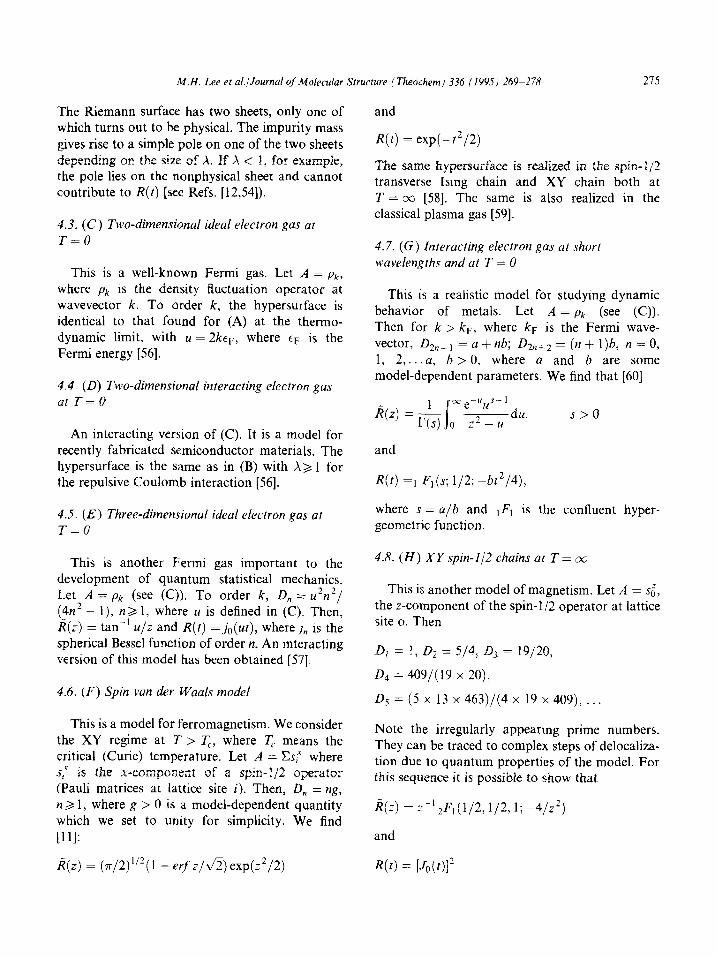
The Riemann surface has two sheets, only one of which turns out to be physical. The impurity mass gives rise to a simple pole on one of the two sheets depending on the size of A. If A < 1, for example, the pole lies on the nonphysical sheet and cannot contribute to R(t) [see Refs. [12,54]).

4.3. (C) Two-dimensional ideal electron gas at r=o

This is a well-known Fermi gas. Let A = pk,

where pk is the density fluctuation operator at wavevector k. To order k, the hypersurface is identical to that found for (A) at the thermo- dynamic limit, with u = 2kcF, where eF is the Fermi energy [56].

4.4. (D) Two-dimensional interacting electron gas atr-o

An interacting version of (C). It is a model for recently fabricated semiconductor materials. The hypersurface is the same as in (B) with X>, 1 for the repulsive Coulomb interaction [56].

4.5. (E) Three-dimensional ideal electron gas at T=U

This is another Fermi gas important to the development of quantum statistical mechanics. Let A = pk (see (C)). To order k, D, = u2n2/ (4n2 - l), nb 1, where u is defined in (C). Then, R(Z) = tan-’ u/z and R(t) =jo(ut), where/, is the spherical Bessel function of order n. An interacting version of this model has been obtained [57].

4.6. (F) Spin van der Waals model

This is a model for ferromagnetism. We consider the XY regime at T > T,, where T, means the critical (Curie) temperature. Let A = Es: where s,~ is the x-component of a spin-l/2 (Pauli matrices at lattice site i). Then, n > 1, where g > 0 is a model-dependent which we set to unity for simplicity. [ll]:

X(Z) = (rr/2)“‘(1 - erfZ/JZ)exp(z2/2)

operalor

4 = w, quantity We find

and

R(t) = exp(-t*/2)

The same hypersurface is realized in the spin-l /2 transverse Ising chain and XY chain both at T = oci [58]. The same is also realized in the classical plasma gas [59].

4.7. (G) Interacting electron gas at short wavelengths and at T = 0

This is a realistic model for studying dynamic behavior of metals. Let A = pk (see (C)). Then for k > kF, where kF is the Fermi wave- vector, D2,,+, = a + nb; D2,,+* = (n + l)b, n = 0, 1, 2,...a, b > 0, where a and b are some model-dependent parameters. We find that [60]

j(z) = -!i s --u s--l

r(s) x%&

0 z*+ u S>O

and

R(t) =I Fl(s; l/2; -bt*/4),

where s = a/b and ,F, is the confluent hyper- geometric function.

4.8. (H) XY spin-112 chains at T = 00

This is another model of magnetism. Let A = sb, the z-component of the spin-l/2 operator at lattice site o. Then

D1 = 1, Dz = 5/4, D> = 19/20,

D4 = 409/(19 x 20),

DS = (5 x 13 x 463)/(4 x 19 x 409), . . .

Note the irregularly appearmg prime numbers. They can be traced to complex steps of delocaliza- tion due to quantum properties of the model. For this sequence it is possible to show that

R(z) = 2-l 2F,(l/2,1/2,1; -4/z’)

and

R(t) = IW12

276 M.H. Lee et al./Journal of Molecular Structure (Theochem) 336 (1995) 269-278

5. Final remarks

We shall now briefly discuss physical situations where the resultant continued fractions are finite (see Appendix D for a list). Finite continued fractions are realized in finite one-dimensional lattice models of spins [61] and harmonic oscillators [62]. (They are also realized in infinite systems, e.g. a one-dimensional homogeneous electron gas [63], higher lattice-dimensional spin models [l 11.) Since these models yield &rite con- tinued fractions, they do not at first appear interesting from the point of view of the analytic theory of continued fractions. However, with increasing degrees of freedom in these models, the continued fractions can be made to grow indefinitely except where localization exists. We find that a limiting dynamic behavior is signaled long before the thermodynamic limit is reached. These finite systems provide a simple way of study- ing the thermodynamic limit process in a dynamic context.

of terminating continued fractions, currently being developed notably by Mtiller and Viswanath [65] and others.

Acknowledgements

Our work has been supported in part by NSF, AR0 and NATO (CRG 921268). We are grateful for their support.

Appendix A: Continued fractions in related areas of physics

If there is a physical localization (i.e. if an excita- tion does not propagate), the continued fractions will remain finite even as the number of particles are increased. For lattice models the localization is uniquely indicated by finite continued fractions.

Continued fractions first appeared in non- equilibrium statistical mechanics in the papers of Mori in the 1960s [5]. However, their underlying origin was left obscure. About two decades later it was clarified that for Hermitian systems these particular continued fractions are a consequence of a realization of Hilbert space [10(b)] i.e. an intrinsic property of that space.

In the previous examples (A)-(H), the hyper- surface was made regular by some special values of the parameters of the models such as T = 0 or co, or short or long wavelengths, referred to as “solvable” models. But for more general values, the hypersurface is not likely to be regular (“nonsolvable” models). For nonsolvable models one can sometimes obtain useful approximate solutions based on solvable models.

Continued fractions can also naturally occur without reference to a particular realized space. Usually they appear if the structure of, say, eigen- values is expressible in a tridiagonal form. A tri- diagonal matrix (Jacobi form) implies a continued fraction, as shown in e.g. Stone’s book [66]. Hence, the origins of continued fractions in other areas are more diverse and perhaps less intrinsic. But the underlying mathematics are similar. We will list below a few related areas where continued fractions have played a significant role. This list is selective. It is meant only to indicate the relevance of continued fractions in physics.

Recall that what determines the time evolution is In solid state physics, Haydock and co-workers the shape of a realized Hilbert space, defined by have used continued fractions as a means of calculat- 0 = (0, D2.. .). If nonsolvable, the space may be ing electronic densities of states [67]. There is an first very roughly described by 0’ = (DIDt.. .), extensive literature [68]. In perturbation theory for where Di, n >2, belong to a related solvable an anharmonic oscillator, for example, the eigen- model. Then somewhat more accurately by values of the Hamiltonian can be constructed in con- c ” = (0, DzDT . .), etc. In this manner one can tinued fractions [69]. Continued fractions have been attempt to obtain a convergent picture. This idea prominent in spectral moments [70], scattering theory was applied to obtain the dynamic structure of an [71], Regge poles [72], relaxation operators [73], Pade electron gas where an ideal electron gas was a sol- approximants [74], etc. When they involve large vable model [64]. We do not discuss other approx- matrices, the Lanczos method has been often used imate solutions, sometimes known under an “art” in diagonalizing these matrices [75].

N.H. Lee et al.lJournal of Molecular Structure (Theochem) 336 (1995) 269-278 211

Appendix B: Kubo scalar product

The Kubo scalar product of a pair of operators X and Y is the inner product of X and Y defined as follows:

(X, Y) =/T’ /:dA(e”HXe-“HYt) - (X)(Yt)

where p is the inverse temperature, t denotes Hermitian conjugation, and the brackets denote an ensemble average, e.g. (X) = Tr(XePaH)/ Tr(eeBH). The physical significance of this inner product is described in Ref. [10(b)]. For its origin, see Ref. [76].

Appendix C: Illustration by RR11

We shall illustrate our method through a simple example. Let p(t) = aO(t) = J,,(t), where Jo is the Bessel function of order 0. It is an admissible function, From Eq. (5b), setting n = 0, we get

D,a, = -al,

= -Jo = J1

where the prime means a differentiation with respect to the argument. Let D1 = u. Then, from Eq. (5b), with n = 1,

D2a2 = -ai + a0

= -J2j2u + (1 - 1/2u)J0

The boundary condition i (see Section 3) implies that u = l/2, i.e. D, = l/Z, hence al = 25,.

Now let D2 = v, i.e. a2 = J2/w. From Eq. (5b), with n = 3,

D3a3 = -u; + al

= -Js/2~ + (2 - 1/2v)J,

The boundary condition i implies that ‘u = l/4, i.e. D2 = l/4 and a2 = 4J2.

Now let D3 = w, i.e. a3 = 2Js/3W. From Eq. (5b), with n = 4,

D4a4 = -a$ + a2

= J&v + (4 - 1/w)J2

Again the boundary condition i implies that w = l/4, i.e. D3 = l/4 and u3 = SJ,. One can proceed in this manner to obtain

D, = 1/2,D2 = D3 =.a. = l/4,

a,(r) = 2”J,(t), n>,O

The continued fraction representation for G(z) is given by the right-hand side of Eq. (2) with the above determined sequence (T = (l/2,1 /4, l/4, . . .). This particular example is realized in a classical harmonic oscillator chain of infinite length and also in a two-dimensional electron gas at T = 0 (see Sections 4.1. and 4.3.).

Appendix D: Finite dimensional Hilbert spaces

Finite dimensional Hilbert spaces are realized in several important physical models with both finite and infinite numbers of particles. One finds that for the topology of these Hilbert spaces their dimensions d are more interesting than their hyper- surfaces u, a reversal from the infinite-dimensional case.

In the single spin model due to Lee [61], one finds both d = 2 and 3. In the one-dimensional homo- geneous electron gas at long wavelengths [63], d = 2. In the harmonic oscillator chain of N molecules [62], d = N + 1. In the spin van der Waals model of N spins [77], d = N, D, = n(N - n). Observe that when N + 00, D,/N = n. The hypersurfaces of N < cx and N = CC are thus substantially different, but become identical only asymptotically. There are other spin models which yield finite-dimensional Hilbert spaces, studied in great detail by Sen [78]. For example, d = 9 + 1, where 9 is the coordination number.

References

[l] H.S. Wall, Analytic Theory of Continued Fractions, Van

Nostrand, New York, 1948.

[2] W.B. Jones and W.J. Thron, Continued Fractions,

Addison Wesley, London, 1980.

[3] R. Askey and M. Ismail, Recurrence Relations, Continued

Fractions and Orthogonal Polynomials, Am. Math. Sot.,

Providence, 1984.

278 M.H. Lee et al./Journal o/Molecular Structure (Theochem) 336 (1995) 269-278

[4] G.A. Baker, Jr., Essential of Pade Approximants, Academic Press, New York, 1975.

[5] (a) H. Mori, Prog. Theor. Phys., 34 (1965) 309. (b) H. Mori, Prog. Theor. Phys., 33 (1965) 423.

[6] R. Zwanzig, Lect. Theor. Phys., Ed. W.E. Brittin, Inter- science, New York, 1961.

[7] A.S.T. Pires, Phys. Status Solidi B, 129 (1985) 163. [8] M.H. Lee, Phys. Rev. Lett. 51, (1985) 1227. [9] M.H. Lee, Phys. Rev. B, 47 (1993) 8293.

E.B. Brown, Phys. Rev. B, 49 (1994) 4305. [lo] (a) M.H. Lee, Phys. Rev. B, 26 (1982) 2547.

(b) M.H. Lee, Phys. Rev. Lett. 49, (1982) 1072. (c) M.H. Lee, J. Math. Phys. 24, (1983) 2512.

[ll] M.H.Lee, I.M. Kim and R. Dekeyser, Phys. Rev. Lett. 52, (1984) 1579.

[12] M.H.Lee,J.FlorencioandJ.Hong,J.Phys.A,22(1989)L331. [13] M.H. Lee, J. Hong and J. Florencio, Phys. Ser., T19 (1987)

498. [14] K.H. Li, Phys. Rep., 134 (1986) 1. [15] A.S.T. Pires, Helv. Phys. Acta, 61 (1988) 988. [16] P. Grigolini, J. Mol. Strut., 250 (1992) 119. [I 71 M. Giordano, P. Grigolini, D. Leporini and P. Marin, Adv.

Chem. Phys., 62 (1985) 321. [18] J. Killingbeck, Rep. Prog. Phys., 48 (1985) 53. [19] M. Cini and A. D’Andrea, J. Phys. C, 21 (1988) 193. [20] T. Uzer, Phys. Rep., 199 (1991) 73. [21] P. Giannozzi, G. Gross0 and G. Pastori Parravicini. Riv.

Nuova Cimento, 13 (1990) 1. [22] P. Braun, Rev. Mod. Phys., 65 (1993) 115. [23] G. Miiller, Phys. Rev. Lett., 60 (1988) 2785. [24] C. Lee and S.I. Koboyashi, Phys. Rev. Lett., 62 (1989)

1061.

[25] D. Vitali and P. Grigolini, Phys. Rev. A, 39 (1989) 1486.

S.N. Yi, J.Y. Ryu and SD. Choi, Prog. Theor. Phys., 82

[26] Z.X. Cai, S. Sen and S.D. Mahanti, Phys. Rev. Lett., 68

(1989) 299.

(1992) 1637. S. Sen, S.D. Mahanti and Z.X. Cai, Phys. Rev. B, 43 (1991) 10990.

[27] R.E. Nettleton, J. Phys. Sot. Jpn., 61 (1992) 3103. [28] R. Tsekov and B. Radoev, J. Phys. Condens. Matter, 4

(1993) L303, 3483. Also see a comment by M.H. Lee, J. Phys. Condens. Matter, 4 (1993) 10487.

[29] N.L. Sharma, Phys. Rev., 45 (1992) 3553. [30] F. Bavaud, J. Stat. Phys., 46 (1987) 753. [31] A.S.T. Pires, Phys. Status Solidi B, 155 (1989) K67. [32] I.M. Kim and B.Y. Ha, Can. J. Phys., 67 (1989) 31. [33] J. Stolze, VS. Viswanath and G. M&r, Z. Phys. B, 89

(1992) 45. [34] CF. Gauss, Comm. Sot. Reg. Goett. Rec., 3 (18 13) 134.

See also Ref. [l], Chapter XVIII. [35] T.J. Stieltjes, Ann. Fat. Sci. Toulouse, 3 (1889) 1; 8 (1894)

1; 9 (1895) 5; Q. J. Math., 24 (1890) 370. [36] L.J. Rogers, Proc. London Math. Sot. (2) 4 (1907) 72. [37] See, e.g., R. Courant, Differential and integral Calculus,

Interscience, New York, 1951, p. 223.

[38] S.W. Lovesey, Condensed Matter: Dynamic Correlations, Benjamin, New York, 1980, p. 15.

[39] H. Falk, Phys. Rev., 165 (1968) 602. [40] R.M. Wilcox, Phys. Rev., 174 (1968) 624. [41] G.A.T. Allan and D.D. Betts, Can. J. Phys., 46 (1968) 799. [42] T. Morita and S. Katsora, J. Phys. C, 2 (1969) 1030. [43] M.H. Lee and 0.1. Sindoni, Phys. Rev. A, 46 (1992)

3028. [44] N.G. van Kampen, Stochastic Processes in Physics and

Chemistry, North-Holland, Amsterdam, 1981, p. 283. [45] W.M. Visscher, Phys. Rev. A, 10 (1974) 2461. [46] D.J. Evans, Physica A, 118 (1983) 51. [47] G. Jacucci, Physica A, 118 (1983) 157. [48] C.M. van Vliet, J. Stat. Phys. 53 (1988) 49. [49] D. Goderis, A. Verbeure and P. Vets, Commun. Math.

Phys., 136 (1991) 265. [50] R. Dekeyser and M.H. Lee, Phys. Rev. B, 43 (1991) 8139. [51] P. Dutta and P.M. Horn, Rev. Mod. Phys. 53 (1981) 497. [52] M.J. Kirton and M.J. Uren, Adv. Phys., 38 (1989) 367. [53] G.Y. Hu and R.F. O’Connell, Phys. Rev. B, 41(1992) 5586. [54] J. Florencio and M.H. Lee, Phys. Rev. A, 31 (1985) 3231. [55] F.G. Goodman, J. Phys. Chem. Solids, 23 (1962) 1491. [56] (a) M.H. Lee and J. Hong, Phys. Rev. Lett., 48 (1982) 634.

(b) M.H. Lee and J. Hong, Phys. Rev. B, 32 (1985) 7734. [57] M.H. Lee and J. Hong, Phys. Rev. B, 30 (1984) 6756. [58] J. Florencio and M.H. Lee, Phys. Rev. B, 35 (1987) 1835. [59] S. Ichimaru, Basic Principles of Plasma Physics, Benjamin.

Reading, 1973. [60] J. Hong and M.H. Lee, Phys. Rev. Lett., 70 (1993) 1972. [61] M.H. Lee, Can. J. Phys., 61 (1983) 428. [62] M.B. Yu, J.H. Kim and M.H. Lee, J. Lumin., 43 (1990)

144 [63] M.H. Lee, J. Hong and N.L. Sharma, Phys. Rev. A, 29

(1984) 1561. [64] J. Hong and M.H. Lee, Phys. Rev. Lett., 55 (1985) 2375. [65] V.S. Viswanath and G. Miiller, The Recursion Method,

Springer, Berlin, 1994. [66] M.H. Stone, Am. Math. Sot., Providence, 1932, p. 530. [67] R. Haydock, Solid State Phys., Ed. H. Ehrenrich, Aca-

demic, New York, 1980. J.F. Annett, W.M.C. Foulkes and R. Haydock, J. Phys. Condens. Matter., 6 (1994) 6455.

1681 D.G. Pettifor and D.L. Wearere (Eds.), The Recursion Method and Its Applications, Springer, Berlin, 1985.

[69] M. Znojil, Phys. Lett. A, 120 (1987) 317. [70] C. Benoit, E. Royer and G. Poussigne, J. Phys. Condens.

Matter., 4 (1992) 3125. [71] J.A. Zuk, Can. J. Phys., 70 (1992) 257. [72] C. Lovelace and D. Masson, Nuova Chim., 26 (1962) 472. [73] P. Giannozzi, G. Grosso, S. Moroni and G. Pastori

Parravicini, Appl. Num. Math., 4 (1988) 273. [74] J. Cizek and E.R. Vrscay, Phys. Rev. A, 30 (1984) 1550. [75] D.M. Young, Comput. Phys. Commun., 53 (1989) 1. [76] R. Kubo, Rep. Prog. Phys., 29 (1966) 255. [77] W.P. Cummings and M.H. Lee, submitted for publication. 1781 S. Sen, Ph.D. Thesis, University of Georgia, 1990.