The thermodynamic design and rating of the heat exchangers ...
291
The thermodynamic design and rating of the heat exchangers for an Aqua-Ammonia absorption-desorption heating and refrigeration cycle JP Botha 22745432 Dissertation submitted in fulfilment of the requirements for the Degree Masters in Mechanical Engineering at the Potchefstroom Campus of the North-West University Supervisor: Prof CP Storm November 2016
Transcript of The thermodynamic design and rating of the heat exchangers ...

The thermodynamic design and rating of the heat exchangers for an Aqua-Ammonia
absorption-desorption heating and refrigeration cycle
JP Botha
22745432
Dissertation submitted in fulfilment of the requirements for the Degree Masters in Mechanical Engineering at the
Potchefstroom Campus of the North-West University
Supervisor: Prof CP Storm
November 2016

Dedicated to the love of my life

- i -
Acknowledgement
The design of the heat exchangers for an aqua-ammonia absorption-desorption cycle would not
have seen the light without the help and support of many people. I would like to make use of this
opportunity to thank all the people who made this oeuvre possible. I would like to express my
sincere gratitude to my mentor, Prof. Chris Storm for the opportunity to complete a study on aqua-
ammonia heat exchangers. Furthermore, I would like to thank Prof. Chris Storm for his guidance
through the course of this design. He not only provided the necessary guidance and allowed me to
develop my own ideas, but also helped improve my people skills. I feel fortunate in getting the
opportunity to work with him. Finally, I would like to thank my fiancée for her love and inspiration,
and my parents for motivating me and keeping my spirits up all the time.

- ii -
Abstract
Title: The thermodynamic design and rating of the heat exchangers for an Aqua-
Ammonia absorption-desorption heating and refrigeration cycle
Author: Jeanré P. Botha
Institution: North-West University: Potchefstroom
Student Number: 22745432
Supervisor: Prof. CP Storm
In today’s day and age the search for more reliable, sustainable, energy efficient systems is a
constant. Over the last three decades large emphasis has been placed on vapour compression
cycles and making them as energy efficient as possible. To increase or decrease the temperature of
a controlled volume requires large amounts of shaft work [kW], however by developing and
conducting research into old technologies it could be possible to obtain a sustainable alternative
heating/cooling system. Aqua-ammonia absorption-desorption cycles are able to operate on
renewable energy, as this process removes the energy hungry compressor from the refrigeration
cycle and replaces it with a generator, absorber, rectifier, and regenerative heat exchanger.
Absorption-desorption cycles are the earliest form of refrigeration cycle, with the earliest dating back
to 1824. Pure ammonia refrigerant is one of only few alternative refrigerants with zero ODP (Ozone
Depletion Potential) and zero GWP (Global Warming Potential) accepted by all governments,
ASHRAE, UNEP, International Institution of Refrigeration, and almost all Institutes of Refrigeration
worldwide (ASHRAE, 1994).
In view of that, an investigation is required into alternative heating/cooling cycles, which can
be adapted and optimised to suit the limitations and requirements of alternative energy sources.
Contained within this dissertation are the thermodynamic and mechanical designs required for the
heat exchangers of an aqua-ammonia absorption-desorption cycle. The study includes an extensive
theoretical background and literature review, which led to the further investigation of the
thermophysical properties of aqua-ammonia refrigerant. Furthermore, the oeuvre includes the
verification and validation of the thermodynamic design and rating model for seven heat
exchangers, which are required to fully optimise the coefficient of performance of the aqua-ammonia
absorption-desorption cycle. The software package MS Excel was used to code the preliminary
thermodynamic design model, after which the software package EES was utilised to verify that the
preliminary thermodynamic design model had no mathematical errors. Validation of the
thermodynamic design models came in the form of predicted overall heat transfer coefficient values
versus typically expected overall heat transfer coefficient ranges. Where the typical Uc ranges have

- iii -
similar or near identical heat exchanger configuration to that of the thermodynamic design models in
this dissertation.
The mechanical design isn’t directly related to the main focus of this study, but does form an
integral part of the overall design of aqua-ammonia heat exchangers and is included in the scope of
work. The mechanical design includes the necessary first principle considerations to ensure the safe
operation of the heating and refrigeration package unit.
Keywords: Aqua-ammonia; absorption-desorption; thermophysical properties; heat exchanger(s);
thermodynamic design; two-phase; turning point; heating and refrigeration.

- iv -
Table of Contents
Chapter 1
1 INTRODUCTION ................................................................................................................... 1
1.1 History of Absorption-Desorption Refrigeration Cycles .................................................... 1
1.2 Background of an Aqua-Ammonia Absorption-Desorption Cycle ..................................... 2
1.3 Rationale for Research .................................................................................................... 5
1.4 Problem Statement .......................................................................................................... 5
1.5 Objectives ....................................................................................................................... 6
1.6 Research Methodology .................................................................................................... 6
Chapter 2
2 LITERATURE REVIEW AND THEORETICAL BACKGROUND STUDY ................................ 8
2.1 Aqua-Ammonia Absorption-Desorption Cycle Components ............................................. 9
2.1.1 Generator (Bubble Pump) and Rectifier (Distiller) .................................................... 9
2.1.2 Condenser ............................................................................................................. 10
2.1.3 Pre-Cool Heat Exchanger ...................................................................................... 10
2.1.4 Venturi Nozzle ....................................................................................................... 10
2.1.5 Evaporator ............................................................................................................. 11
2.1.6 Absorber ................................................................................................................ 11
2.1.7 Regenerative Heat Exchanger ............................................................................... 12
2.2 Heat Exchanger Classification ....................................................................................... 12
2.2.1 Tubular Heat Exchangers ...................................................................................... 13
2.2.2 Influence of Working Fluids .................................................................................... 14
2.3 Thermophysical Properties of Aqua-Ammonia Solutions ............................................... 15
2.3.1 Introduction to the Thermophysical Properties of Aqua-Ammonia Solution ............ 15
2.4 Thermophysical Properties of Ethylene Glycol-Water Solutions .................................... 16
2.5 Thermodynamic Design and Rating ............................................................................... 16
2.5.1 Basics of Heat Exchanger Design Calculations ..................................................... 17

- v -
2.5.2 Log Mean Temperature Difference Method (LMTD Method) .................................. 17
2.5.3 The Effectiveness Method (NTU Method) .............................................................. 19
2.5.4 Overall Heat Transfer Coefficient ........................................................................... 20
2.5.5 Shell Side Heat Transfer Coefficient ...................................................................... 21
2.5.6 Tube Side Heat Transfer Coefficient ...................................................................... 26
2.5.7 Heat Transfer Surface Area ................................................................................... 28
2.6 Extended Theoretical Background and Literature Review ............................................. 28
2.7 Conclusion .................................................................................................................... 29
Chapter 3
3 THERMOPHYSICAL PROPERTIES AND THERMODYNAMIC DESIGN SELECTION ....... 30
3.1 Thermophysical Properties for Aqua-Ammonia Solutions .............................................. 31
3.1.1 Aqua-Ammonia Two-Phase Condensation Investigation........................................ 32
3.1.2 Thermophysical Properties of State 3 to 5 ............................................................. 36
3.1.3 Thermophysical Properties of State 7 to 8 ............................................................. 44
3.1.4 Thermophysical Properties of Weak and Strong Aqua-Ammonia Solutions ........... 47
3.1.5 Conclusion of Thermophysical Properties of Aqua-Ammonia Solutions ................. 48
3.2 Extended Chapter 3 – Thermophysical Properties and Thermodynamic Design
Selection ....................................................................................................................... 48
3.3 Conclusion .................................................................................................................... 49
Chapter 4
4 THERMODYNAMIC DESIGN AND RATING ....................................................................... 50
4.1 Overview of the Experimental Setup .............................................................................. 51
4.2 Introduction to the Heating Side Heat Exchangers (State 3 to 5) ................................... 52
4.3 Stage 1 Condenser (State TP to 5) ................................................................................ 55
4.3.1 Preliminary Thermodynamic Design ...................................................................... 55
4.3.2 Performance Rating of the Thermodynamic Design ............................................... 61
4.3.3 Thermodynamic Design Verification ...................................................................... 62
4.3.4 Design Sizing Selection ......................................................................................... 64
4.4 Stage 2 Condenser (State 4 to TP) ................................................................................ 65

- vi -
4.4.1 Preliminary Thermodynamic Design ...................................................................... 65
4.4.2 Performance Rating of the Thermodynamic Design ............................................... 68
4.4.3 Thermodynamic Design Verification ...................................................................... 70
4.4.4 Design Sizing Selection ......................................................................................... 71
4.5 De-superheating Condenser (State 3 to 4) .................................................................... 71
4.5.1 Preliminary Thermodynamic Design ...................................................................... 71
4.5.2 Performance Rating of the Thermodynamic Design ............................................... 73
4.5.3 Thermodynamic Design Verification ...................................................................... 74
4.5.4 Design Sizing Selection ......................................................................................... 75
4.6 Pre-Cool Heat Exchanger (State 5 to 6 & 9 to 10) ......................................................... 75
4.6.1 Preliminary Thermodynamic Design ...................................................................... 76
4.6.2 Performance Rating of the Thermodynamic Design ............................................... 77
4.6.3 Thermodynamic Design Verification ...................................................................... 77
4.6.4 Design Sizing Selection ......................................................................................... 78
4.7 Venturi Nozzle and Orifice (State 6 to 7) ........................................................................ 78
4.7.1 Venturi Nozzle – Thermodynamic Design .............................................................. 79
4.7.2 Orifice – Thermodynamic Design Sizing ................................................................ 81
4.8 Evaporator (State 8 to 9) ............................................................................................... 81
4.8.1 Preliminary Thermodynamic Design ...................................................................... 82
4.8.2 Performance Rating of the Thermodynamic Design ............................................... 86
4.8.3 Thermodynamic Design Verification ...................................................................... 86
4.8.4 Design Sizing Selection ......................................................................................... 87
4.9 Auxiliary-Regenerative Heat Exchanger (Weak and Strong Aqua-Ammonia
Solutions) ...................................................................................................................... 87
4.9.1 Regenerative Heat Exchanger – Preliminary Thermodynamic Design ................... 88
4.9.2 Regenerative Heat Exchanger – Performance Rating of the Thermodynamic
Design ................................................................................................................... 89
4.9.3 Regenerative Heat Exchanger – Thermodynamic Design Verification ................... 89
4.9.4 Regenerative Heat Exchanger – Design Selection................................................. 90
4.9.5 Auxiliary Heat Exchanger – Preliminary Thermodynamic Design ........................... 91
4.9.6 Auxiliary Heat Exchanger – Performance Rating of the Thermodynamic Design ... 92
4.9.7 Auxiliary Heat Exchanger – Thermodynamic Design Verification ........................... 92
4.9.8 Auxiliary heat exchanger – Design Sizing Selection ............................................... 93
4.10 Conclusion .................................................................................................................... 93
- vii -
Chapter 5
5 THERMODYNAMIC DESIGN VALIDATION ........................................................................ 95
5.1 Thermodynamic Design Validation Process .................................................................. 96
5.2 Stage 1 Condenser ....................................................................................................... 97
5.2.1 Tube Side Heat Transfer Coefficient Correlation Limitations .................................. 98
5.2.2 Shell Side Heat Transfer Coefficient Correlation Limitations .................................. 99
5.2.3 Overall Heat Transfer Coefficient Validation Results .............................................. 99
5.2.4 Shell Side Heat Transfer Coefficient Validation Results ....................................... 105
5.2.5 Thermodynamic Design Validation Conclusion .................................................... 106
5.3 Stage 2 Condenser ..................................................................................................... 107
5.3.1 Overall Heat Transfer Coefficient Validation Results ............................................ 108
5.3.2 Thermodynamic Design Validation Conclusion .................................................... 110
5.4 De-superheating Condenser ........................................................................................ 111
5.4.1 Overall Heat Transfer Coefficient Validation Results ............................................ 111
5.4.2 Thermodynamic Design Validation Conclusion .................................................... 113
5.5 Pre-Cool Heat Exchanger ............................................................................................ 113
5.5.1 Shell Side Heat Transfer Coefficient Validation Results ....................................... 113
5.5.2 Thermodynamic Design Validation Conclusion .................................................... 114
5.6 Evaporator ................................................................................................................... 115
5.6.1 Overall Heat Transfer Coefficient Validation Results ............................................ 115
5.6.2 Convective Boiling Heat Transfer Coefficient Validation Results .......................... 117
5.6.3 Thermodynamic Design Validation Conclusion .................................................... 118
5.7 Auxiliary-Regenerative Heat Exchanger ...................................................................... 119
5.7.1 Regenerative Heat Exchanger – Overall Heat Transfer Coefficient Validation
Results ................................................................................................................ 120
5.7.2 Auxiliary Heat Exchanger – Overall Heat Transfer Coefficient Validation
Results ................................................................................................................ 121
5.7.3 Aux-Regen Heat Exchanger – Thermodynamic Design Validation Conclusion .... 122
5.8 Conclusion .................................................................................................................. 123

- viii -
Chapter 6
6 CLOSURE ......................................................................................................................... 124
6.1 Conclusions ................................................................................................................. 125
6.2 Recommendations ...................................................................................................... 126
Annexure
LIST OF REFERENCES ............................................................................................................. 128
APPENDIX A – Extended Chapter 2 – Literature Review and Theoretical Background Study
APPENDIX B – Extended Chapter 3 – Thermophysical Properties
APPENDIX C – Concept Design Generation and Evaluation
APPENDIX D – Extended Chapter 4 – Thermodynamic Design and Rating
APPENDIX E – Mechanical Considerations and Design

- ix -
List of Figures
Chapter 1
Figure 1.1: Basic schematic of an absorption-desorption system (Stoecker & Jones, 1983). .......... 3
Figure 1.2: Basic component representation of an Aqua-ammonia absorption-desorption cycle
(Stoecker & Jones, 1983). ............................................................................................ 3
Figure 1.3: Schematic representation of the components within an aqua-ammonia absorption-
desorption heating & refrigeration cycle. ....................................................................... 5
Chapter 2
Figure 2.1: Control volume diagram of a venturi (Engineeringtoolbox, 2015). ............................... 11
Figure 2.2: Double-pipe heat exchanger (Britannica, 2006). ......................................................... 13
Figure 2.3: Shell and tube heat exchanger (HRS Heat Exchangers, 2016). .................................. 14
Figure 2.4: Film condensation flow profile on a horizontal tube (Kakac & Liu, 2002). .................... 23
Figure 2.5: Graphic representation of condensate flow through tube bundles (Kakaç & Liu, 2002).23
Chapter 3
Figure 3.1: Aqua-ammonia absorption-desorption heating and refrigeration heat exchangers
temperature vs. enthalpy diagram. .............................................................................. 31
Figure 3.2: Weak and strong solutions aqua-ammonia temperature vs. enthalpy diagram. ........... 32
Figure 3.3: Temperature vs. enthalpy of state 3 to 5 for three ambient design conditions. ............ 33
Figure 3.4: Enthalpy vs. quality of the two-phase region for three ambient design conditions of aqua-
ammonia. .................................................................................................................... 34
Figure 3.5: Temperature vs. quality of the two-phase region for three ambient design conditions of
aqua-ammonia. ........................................................................................................... 34
Figure 3.6: Linear enthalpy vs. quality estimation of aqua-ammonia in the two-phase region and the
graphical representation of the ‘turning point’. ............................................................ 35
Figure 3.7: Density vs. quality for aqua-ammonia in the two-phase region of three ambient design
conditions. .................................................................................................................. 42
Figure 3.8: Linear enthalpy estimation of aqua-ammonia at 236.39 [kPa]. .................................... 44

- x -
Figure 3.9: Temperature vs. enthalpy of the auxiliary and regenerative heat exchangers. ............ 47
Chapter 4
Figure 4.1: Schematic representation of the housing structure for the solar-driven aqua-ammonia
absorption-desorption heating & refrigeration package unit. ....................................... 51
Figure 4.2: Schematic representation of the refrigerant and coolant flow diagram with the heating
side components. ....................................................................................................... 53
Figure 4.3: Evaporator Inlet Schematic Component Diagram ........................................................ 79
Figure 4.4: Schematic representation of the refrigeration side components. ................................. 82
Chapter 5
Figure 5.1: Stage 1 Condenser - Overall heat transfer coefficient vs. tube side Reynolds number
simulation model output plot. .................................................................................... 100
Figure 5.2: Temperature vs. enthalpy of different mass concentrations of ammonia in water
mixtures. ................................................................................................................... 102
Figure 5.3: Enthalpy vs. quality investigation of ‘turning point’ for 0.9 and 0.99 mass concentrations
ammonia in water. .................................................................................................... 103
Figure 5.4: Stage 1 condenser – Shell side heat transfer coefficient vs. temperature difference
simulation model output plot. .................................................................................... 105
Figure 5.5: Stage 2 condenser – Overall heat transfer coefficient vs. shell side Reynolds number
simulation model output plot. .................................................................................... 108
Figure 5.6: De-superheating condenser – Overall heat transfer coefficient vs. shell side Reynolds
number simulation model output plot. ....................................................................... 112
Figure 5.7: Pre-Cool heat exchanger – Shell side heat transfer coefficient vs. shell side Reynolds
number simulation model output plot. ....................................................................... 114
Figure 5.8: Evaporator – Overall heat transfer coefficient vs. tube side Reynolds number simulation
model output plot. ..................................................................................................... 116
Figure 5.9: Evaporator – Convective boiling heat transfer coefficient vs. shell side liquid film
Reynolds numbers. ................................................................................................... 118
Figure 5.10: Regenerative heat exchanger – Overall heat transfer coefficient vs. shell side Reynolds
number simulation model output plot. ....................................................................... 120

- xi -
Figure 5.11: Auxiliary heat exchanger – Overall heat transfer coefficient vs. shell side Reynolds
number simulation model output plot. ....................................................................... 122

- xii -
List of Tables
Chapter 2
Table 2.1: Effectiveness relations of (Kays & Perkins, 1972). ....................................................... 20
Table 2.2: Nusselt number correlations for flow over tube bundles for NL > 16.............................. 22
Table 2.3: Correction factors cn. .................................................................................................... 22
Table 2.4: Tube pass constant (Kakaç & Liu, 2002). ..................................................................... 28
Table 2.5: Tube bundle layout constant (Kakaç & Liu, 2002). ....................................................... 28
Chapter 3
Table 3.1: Enthalpy output values for thermodynamic states 3, 4, TP, & 5. ................................... 37
Table 3.2: Thermophysical properties of pure ammonia and water for state 3. ............................. 39
Table 3.3: Thermophysical properties of aqua-ammonia for state 3. ............................................. 40
Chapter 4
Table 4.1: Stage 1 condenser – Thermodynamic design input parameters. .................................. 55
Table 4.2: Stage 2 condenser – Thermodynamic design input parameters. .................................. 65
Table 4.3: State 4 thermophysical properties for winter ambient conditions. ................................. 66
Table 4.4: State TP thermophysical properties for winter ambient conditions. ............................... 66
Table 4.5: Stage 2 condenser – Pressure drop. ............................................................................ 70
Table 4.6: Stage 2 condenser – EES verification output parameters. ............................................ 70
Table 4.7: De-superheating condenser – Thermodynamic design input parameters. .................... 71
Table 4.8: De-superheating condenser – Preliminary thermodynamic design output parameters. 72
Table 4.9: De-superheating condenser – Pressure drop. .............................................................. 74
Table 4.10: De-superheating condenser – EES verification output parameters. ............................ 74
Table 4.11: Pre-cool heat exchanger – Thermodynamic design input parameters. ....................... 76
Table 4.12: Pre-cool heat exchanger – Preliminary design output parameters. ............................. 76
Table 4.13: Pre-cool heat exchanger – Performance rating. ......................................................... 77

- xiii -
Table 4.14: Pre-cool heat exchanger – EES verification output parameters. ................................. 78
Table 4.15: Venturi nozzle design input parameters. .................................................................... 80
Table 4.16: Orifice design output parameters. .............................................................................. 81
Table 4.17: Evaporator – Thermodynamic design input parameters. ............................................ 82
Table 4.18: Evaporator – Tube side heat transfer coefficient. ....................................................... 85
Table 4.19: Evaporator – Thermodynamic design output parameters. .......................................... 86
Table 4.20: Evaporator – Performance rating. .............................................................................. 86
Table 4.21: Evaporator – EES verification output parameters. ...................................................... 87
Table 4.22: Regenerative heat exchanger – Thermodynamic design input parameters. ............... 88
Table 4.23: Regenerative heat exchanger – Preliminary design output parameters. ..................... 89
Table 4.24: Regenerative heat exchanger – Performance rating. ................................................. 89
Table 4.25: Regenerative heat exchanger – EES verification output parameters. ......................... 90
Table 4.26: Regenerative heat exchanger – Tube lengths. ........................................................... 90
Table 4.27: Auxiliary heat exchanger – Thermodynamic design input parameters. ....................... 91
Table 4.28: Auxiliary heat exchanger – Preliminary thermodynamic design output parameters. ... 91
Table 4.29: Auxiliary heat exchanger – Performance rating. ......................................................... 92
Table 4.30: Regenerative heat exchanger – EES verification output parameters. ......................... 93
Table 4.31: Summative thermodynamic design table of the heat exchangers for an aqua-ammonia
absorption-desorption heating and refrigeration cycle. ................................................ 94
Chapter 5
Table 5.1: Typical ranges of overall heat transfer coefficients for shell and tube heat exchangers. 96
Table 5.2: Typical ranges of heat transfer coefficients for shell and tube heat exchangers. .......... 97
Table 5.3: Stage 1 condenser - The initial boundary conditions for 3 permutations of working fluids.
................................................................................................................................. 101
Table 5.4: Stage 1 condenser - The limit boundary conditions for 3 permutations of working fluids.
................................................................................................................................. 102
Table 5.5: The comparison table of the stage 1 condenser simulation model with 90 & 99 wt% aqua-
ammonia and water as coolant. ................................................................................ 104
Table 5.6: Stage 1 condenser – Shell side heat transfer coefficient output values. ..................... 106
Table 5.7: Stage 2 condenser – Tube side heat transfer coefficient correlation limitations. ......... 107

- xiv -
Table 5.8: Stage 2 condenser – Shell side heat transfer coefficient correlation limitations. ......... 108
Table 5.9: Stage 2 Condenser – Overall heat transfer coefficient vs. shell side Reynolds numbers
simulation model output values. ................................................................................ 109
Table 5.10: The comparison table of the sized stage 2 condenser model with 90 & 99 wt% aqua-
ammonia and ethylene glycol water as coolant. ........................................................ 110
Table 5.11: De-superheating condenser – Tube side heat transfer coefficient correlation limitations.
................................................................................................................................. 111
Table 5.12: De-superheating condenser – Shell side heat transfer coefficient correlation limitations.
................................................................................................................................. 111
Table 5.13: De-superheating condenser – Overall heat transfer coefficient vs. shell side Reynolds
numbers simulation model output values. ................................................................. 112
Table 5.14: Pre-cool heat exchanger – Shell side heat transfer coefficient correlation limitations.113
Table 5.15: Evaporator – Tube side heat transfer coefficient correlation limitations. ................... 115
Table 5.16: Evaporator – Overall heat transfer coefficient vs. tube side Reynolds number simulation
model output values.................................................................................................. 117
Table 5.17: Tube side heat transfer coefficient correlation limitations. ........................................ 119
Table 5.18: Shell side heat transfer coefficient correlation limitations. ......................................... 120
Table 5.19: Regenerative heat exchanger – Overall heat transfer coefficient vs. shell side Reynolds
number simulation model output values. ................................................................... 121
Table 5.20: Auxiliary heat exchanger – Overall heat transfer coefficient vs. shell side Reynolds
number simulation model output values. ................................................................... 122
- xv -
Nomenclature
Acs Bundle cross flow area m2
As Heat transfer surface area m2
B Baffle spacing m
c Capacity ratio -
C Clearance m
Ccr Heater geometry constant -
Cp Specific thermal capacity J/kg.K
Cn Heat transfer coefficient correction factor -
Csf Surface-fluid combination constant -
COP Coefficient of performance -
d Diameter m
De Equivalent diameter m
Ds Inner shell diameter m
F Force N
Fc Log mean temperature difference correction factor -
g Gravitational acceleration m/s2
Gs Mass velocity kg/m2.s
Gz Graetz number -
h Heat transfer coefficient W/m2.K
k Thermal conductivity W/m.K
L Length m
Lt Heat transfer tube length m
M Molar kg/k.mol
Mass flow rate kg/s
NL Number of tube rows -
Np Number of tube passes -
Nt Number of tubes -
Nu Nusselt number -
NTU Number of transfer units -
P Pressure Pa
PD Design pressure Pa
PT Pitch size m
Pe Pèclet number -
Pr Prandtl number -

- xvi -
PR Pitch ratio -
Q Quality -
Heat transfer rate W
r Radius m
Re Reynolds number -
t Wall thickness m
T Temperature °C or K
u Velocity m/s
Uc Overall heat transfer coefficient W/m2.K
Uf Fouling overall heat transfer coefficient W/m2.K
Volume flow rate m3/s
x Mass concentration kg/kg
y Molar concentration k.mol/k.mol
Greek Symbols
α Enthalpy J/kg
δ Film thickness m
ε Effectiveness -
θ General thermophysical property variable -
μ Dynamic viscosity kg/m.s
ρ Density kg/m3
σ Stress Pa
φ Circumferential angle rad
Δ Delta or difference -
Σ Sum of -

- xvii -
Subscripts
fg Latent
b Bulk
c Cold
cb Convective boiling
CF Counter-flow
clnt Coolant
crit Critical
DSN Average ambient design conditions
est Estimation
h Hot
i or in In
l Saturated liquid
LMTD Log mean temperature difference
m Mean
max Maximum
min Minimum
mix Mixture
nb Nucleate boiling
o or out Out
PF Parallel-flow
s or S Shell side
sat Saturation
sh Shear
SMR Summer ambient design conditions
ss Strong aqua-ammonia solution
t or T Tube side
TP Turning Point
v Saturated vapour
WRT Winter ambient design conditions
ws Weak aqua-ammonia solution
XF Cross-flow

- xviii -
Abbreviations
ABS Absorber
Aux Auxiliary heat exchanger
BP Bubble pump generator
CAD Computer aided design
DHC De-superheating condenser
EES Engineering equation solver
Evap Evaporator
HTC Heat transfer coefficient
HTEX Heat exchanger
H&R Heating and refrigeration
IAWPS International Association for the Properties of Water and Steam
LMTD Log mean temperature difference
MTD Mean temperature difference
PC Pre-cool heat exchanger
Regen Regenerative heat exchanger
S1C Stage 1 Condenser
S2C Stage 2 Condenser

- 1 -
Chapter 1
1 INTRODUCTION
Summary
In today’s day and age the search for low-energy consuming and environmentally friendly systems
are a constant. This could not be more relevant to a struggling energy sector of South Africa and
the global need to shift energy requirements from fossil energy sources onto alternative energy
sources, which would lead to positive effects on the environment and stimulate economic growth. A
large consumer of electrical energy is temperature manipulation in a controlled volume, which
requires large amounts of shaft work [kW] to increase or decrease the temperature. The most
difficult temperature manipulation is the removal of heat, known as refrigeration. Thus, an
investigation is needed into alternative heating/cooling cycles, which can be adapted and optimised
to suit the limitations and requirements of alternative energy sources. South Africa is one of only a
few countries blessed with high levels of solar irradiation all year round, and would be a prime
candidate for investigating a solar-powered heating/cooling cycle. One such alternative
heating/cooling cycle that utilises heat energy is an absorption-desorption cycle.

Chapter 1: Introduction
- 1 -
1.1 History of Absorption-Desorption Refrigeration Cycles
Refrigeration is well known to just about every person on earth, as “the machine keeping my food
cold”. This is due to the globalisation during the early 20th century of the household refrigerator and
its commercial applicant in food stores. Refrigeration can be described as the transfer of heat from
the surroundings to a chamber with an absence of heat.
Thus, refrigeration’s most important application is the preservation of food. Most foods kept
at room temperature will spoil rapidly, which is due to the rapid growth of bacteria. Refrigerators
preserve food by maintaining the food at an optimum temperature of 4 [°C], which is low enough to
halter the growth of bacteria, but high enough that there aren’t any ice crystallisations within the
food (Althouse et al., 1992).
The history of refrigeration started with continuous consumption refrigeration, whereby a
cooling effect is obtained by utilising elementary refrigerants, such as melting ice or sublimation of
solid carbon dioxide (dry-ice) at atmospheric pressure. Today, the most common form of
refrigeration is the vapour compression cycle, which utilises a continuous cycle of its working fluid,
known as a refrigerant. Although vapour compression cycles are the most popular form of
refrigeration cycles today, these weren’t the earliest refrigeration cycles. Absorption-desorption
cycles are the earliest form of refrigeration cycle dating back to 1824 (Althouse et al., 1992). Solid
absorption systems operate on the principle discovered by Michael Faraday in the early 1820’s.
Through experiments Faraday succeeded in liquefying ammonia, which scientists had
believed to be a fixed gas, by exposing the ammonia vapour to silver chloride powder. After the
vapour has been absorbed by the silver chloride, heat was applied and a liquid solution was the
product. Edmond Carré developed the first absorption machine in 1850, by using sulphuric acid
and water solution (Althouse et al., 1992). It was only his brother Ferdinand Carré who
demonstrated an ammonia-water refrigeration machine in 1859; later in 1860 he received the first
U.S. patent for a commercial absorption unit. ‘Serve Electrically’ was founded in 1902 as the
Hercules Buggy Works and became a manufacturer of electric refrigerators, the company is known
as Servel. Servel purchased the US rights to a new AB Electrolux gas heat driven absorption
refrigerator invented by a couple of Swedish engineering students, Carl G. Munters and Baltzar
von Platen during the 1930’s. The production of the AB Electrolux absorption refrigerator stretched
from 1926 to the early 1950’s (Thevenot, 1979).
Absorption-desorption systems have experienced ups and downs over the years. The
absorption-desorption cycle was the predecessor to the vapour-compression cycle in the late
nineteenth century. Absorption-desorption systems were used in domestic refrigerators and as
refrigeration for large chemical and process industries. Prices of natural gas, fuel availability and
governmental policies caused the decline in sales of absorption-desorption refrigerators during the
mid-1970’s in the USA (Forley, 2000), although Asian countries with electricity shortages have

Chapter 1: Introduction
- 2 -
shown an increase in sales since the mid-1970’s. Absorption-desorption refrigeration hit its peak in
1981 with two absorption-desorption plants created by former USSR Borsig GmbH, which had a
cooling capacity of 22.1 [MW] at -5 [°C] in the evaporator (Srikhirin et al., 2001).
However, in the late 20th century focus shifted to vapour compression cycles, and absorption-
desorption cycle technology was shelved due to the assumption that the cycle has a high power
consumption and low overall efficiency. Now, at the turn of the century the assumption has been
re-evaluated, where it was found that both cycles waste similar amounts of energy. Where the
vapour compression cycle uses electricity generated at around 35% efficiency in power plants, and
absorption-desorption cycles uses heat energy. When the 35% efficiency of power stations are
factored into the overall efficiency of vapour compression cycles, then, the two cycles become
comparable (Srikhirin et al., 2001). Thus, it can be assumed that absorption-desorption cycle
technology could be economically viable in areas with energy concerns.
Coefficient of Performance
When dealing with the coefficient of performance of an absorption-desorption cycle, a different
approach is needed to that of the vapour compression cycle. Thus, for the absorption-desorption
cycle the coefficient of performance as proposed by (Stoecker & Jones, 1983) can be expressed
as:
(1.1)
with
≡ Refrigeration capacity [kW]
≡ Heat added to the generator [kW]
The values of COPabs for aqua-ammonia are commonly 0.7 compared to the commonly obtained
COP of 3 to 4 for vapour compression cycle, although the coefficient of performance of the heating
capacity should also be taken into account for the absorption-desorption cycle (Stoecker & Jones,
1983). The values of heating capacity COPabs are commonly between 1.5 to 1.7, thus, it can be
concluded that the absorption-desorption cycle fully utilises its heat source input, whether it be
solar- or industrial waste heat energy.
1.2 Background of an Aqua-Ammonia Absorption-Desorption Cycle
Absorption-desorption cycles have two great advantages, namely, the cycle requires no rotating
mechanical components and any heat source to power the generator component. Even low grade
industrial waste heat can be utilised to power the generator in an absorption-desorption cycle. This
is due to the natural circulation of the working fluid within the absorption-desorption cycle, also

Chapter 1: Introduction
- 3 -
known as Gibbs free energy (Stoecker & Jones, 1983). Figure 1.1 illustrates the fundamental
component cycle of an absorption-desorption cycle, but more specifically that of a LiBr-water cycle.
Thus for the purpose of this dissertation, focus will be kept on aqua-ammonia absorption-
desorption cycles.
Figure 1.1: Basic schematic of an absorption-desorption system (Stoecker & Jones, 1983).
An aqua-ammonia absorption-desorption cycle requires the addition of two extra
components, namely, the rectifier and the analyser. The purposes of these components are to
remove the unwanted water vapour content from the refrigerant vapour, which is released by the
generator. The positioning of the above mentioned components are illustrated in Fig. 1.2, along
with all other fundamental components of an aqua-ammonia absorption-desorption cycle.
Figure 1.2: Basic component representation of an Aqua-ammonia absorption-desorption cycle (Stoecker & Jones, 1983).

Chapter 1: Introduction
- 4 -
The generator/bubble pump component is where the desorption process of the cycle takes
place. Here the refrigerant absorbent pair is separated, though the addition of heat, which in effect
boils the refrigerant off of the strong concentrated aqua-ammonia solution. This process creates a
high concentrated vapour refrigerant, which next enters the rectifier.
The rectifier is a contact counter current water vapour remover. The refrigerant vapour that
is driven off by the generator flows through a series of staggered stacked plates. The plates simply
let weak solution aqua-ammonia dribble down collecting any water, be it liquid or vapour. The
analyser is a closed water cooled heat exchanger, with the function of condensing water vapour
out of the near pure ammonia solution, with the water flowing back into the rectifier.
High pressure pure ammonia vapour flows to the condenser, where the refrigerant is
condensed into a high pressure liquid. Condensation is achieved by the removal of heat by the
much ‘colder’ coolant fluid. The coolant temperature raises to an effective percentage of that of the
refrigerant, the coolant can now be used in the means of heating purposes. The high pressure
liquid refrigerant flows through an expansion valve, whereby the pressure drops slightly. The
pressure doesn’t drop as dramatically as that of the vapour compression cycle, due to the
absorption-desorption cycle circulating with Gibbs free energy. The dramatic drop in ‘pressure’ is
caused by the addition of an auxiliary gas, i.e. Hydrogen or Helium. The presence of an auxiliary
gas causes the refrigerant to have a very low partial pressure, which in turn is the same effect as
that of the vapour compression cycle. The refrigerant then enters the evaporator, where heat is
added to evaporate or more commonly known boil the refrigerant to a state of saturated vapour.
The exchange of heat within the evaporator is simply put, where refrigeration happens.
The low partial pressure saturated vapour ammonia is sucked from the evaporator to the
absorber, the suction is caused by the high affinity ammonia and water have for one another.
Weak solution aqua-ammonia and high concentration saturated ammonia react exothermically to
form a strong aqua-ammonia solution. The strong solution returns back to the generator, passing
through a heat exchanger, known as, the regenerator. A regenerator is fundamental to the aqua-
ammonia absorption desorption cycle, with the main purpose of lowering the temperature of the
weak solution entering the absorber is to increase the concentration of the strong solution exiting
the absorber.
The component diagram represented by Fig. 1.3 is a basic illustration of the aqua-ammonia
absorption-desorption cycle used for this study, with the addition of two pre-coolers, namely, the
de-superheating condenser and pre-cool heat exchanger. The component diagram also represents
the layout of the heat exchangers and the path of the primary refrigerant. These components are
placed at different height intervals to optimise the buoyancy forces to circulate the refrigerant.

Chapter 1: Introduction
- 5 -
Figure 1.3: Schematic representation of the components within an aqua-ammonia absorption-desorption heating & refrigeration cycle.
1.3 Rationale for Research
This study forms part of a larger research project that seeks to experimentally test an aqua-
ammonia absorption-desorption heating and refrigeration package unit that utilises solar irradiation
to power the heat source required in the bubble pump generator. Multiple sources are available for
the thermodynamic design and rating of heat exchangers, but very few or out-dated sources are
available for the thermodynamic design and rating of aqua-ammonia heat exchangers. The out-
dated sources of thermodynamic design for aqua-ammonia heat exchangers are based on the
assumption that the working fluid is a pure substance and not on an aqueous ammonia solution.
Research is specifically required into the thermodynamic design and rating of heat exchangers
utilizing aqua-ammonia in the ambiguous two-phase and superheated vapour regions. As this
study is interwoven into the larger project it’s largely dependent on the progress of other studies
being conducted coherently, which may halter the progress of this study.
1.4 Problem Statement
An investigation into the thermodynamic design and rating of all of the heat exchangers in an aqua-
ammonia absorption-desorption cycle is required to complete the experimental setup of the heating
and refrigeration package unit. This directly ties into the investigation of alternative heating/cooling
cycles as the heat exchangers of an absorption-desorption cycle play a fundamental role in making
the cycle function at its optimum. The heat exchangers must be designed to adapt to the limitations
and requirements of alternative energy sources.

Chapter 1: Introduction
- 6 -
1.5 Objectives
The purpose of this study is to investigate the thermodynamic design and rating for shell and tube
heat exchangers used in an experimental solar-powered aqua-ammonia absorption-desorption
heating and refrigeration (H&R) package unit. The study aims to develop a software based
thermodynamic design and rating model of the condenser, pre-cool heat exchanger, evaporator,
and regenerative heat exchanger for the specific use in an aqua-ammonia absorption-desorption
H&R package unit or refrigeration cycles with laminar flow regime mass flow rates. The
development of the thermodynamic design and rating model will require verification and validation
to ensure that the heat exchangers are sized accurately, and practically viable. The
thermodynamic design and rating model should comply with the requirements and limitations that a
solar-powered aqua-ammonia absorption-desorption heating and refrigeration package unit entails.
This includes the optimal type and number of heat exchangers required to produce a heating
capacity COP of 1.3 and a cooling capacity COP of 0.7, with 1.5 [kW] heating capacity and 0.8
[kW] cooling capacity.
This study aims to utilise the thermodynamic design and rating model to complete the
mechanical design of the heat exchangers for an aqua-ammonia absorption-desorption cycle. The
mechanical design will include first order principles to ensure the safe operation of the heat
exchangers. Furthermore, the mechanical design will include a full set of manufacturing and
assembly drawings of each heat exchanger and its non-standard components.
1.6 Research Methodology
In the beginning of any research project it’s fundamental to gain knowledge on the subject matter.
Therefore, the first step is to compile a comprehensive literature and theoretical background study
on aqua-ammonia, absorption-desorption refrigeration cycles, and the thermodynamic design and
rating of heat exchangers. Investigation into the behavioural characteristics of aqua-ammonia
refrigeration cycles and its thermophysical properties are required to complete an accurate and
satisfactory thermodynamic design model.
Convention dictates that a functional analysis is required before the design requirements
and specifications, but to keep the oeuvre concise the functional analysis can be construed from
the comprehensive literature review and theoretical background study, and thermophysical
property investigation of aqua-ammonia absorption-desorption refrigeration cycles to form the
design requirements. The design requirements will be ranked according to its level of importance
and utilised in a concept design evaluation matrix.
The software package Microsoft Excel (MS Excel) will be utilised for the preliminary
thermodynamic design model with the Engineering Equation Solver (EES) used to verify that there
are no mathematical errors in the MS Excel thermodynamic design model. The MS Excel

Chapter 1: Introduction
- 7 -
thermodynamic design model must accommodate multiple design-sizing options, in other words
the design model must have multiple shell and tube diameters that generate an array of heat
exchanger designs to choose from. Furthermore, the MS Excel thermodynamic design model must
incorporate the option of multiple design layouts, for instance single or double tube pass, 45° or
60° tube bundle layout. The preliminary design criteria will be based on the thermal heat
exchanger efficiency, the tube length over shell diameter ratio (2 < L/Ds < 7), and the number of
tubes (2 < Nt < 100). The thermal efficiency of each heat exchanger will be measured using the
NTU-effectiveness method and standardised counter- or cross-flow NTU vs. effectiveness curves.
The thermal efficiency should be as close to the theoretical maximum as possible. The NTU-
effectiveness method will fulfil another important duty, which is determining whether the assumed
outlet temperature of the secondary fluid is satisfactory in accordance to a real world heat
exchanger scenario.
After the thermodynamic design model of each heat exchanger is verified, the validation
process can commence. The validation process will prove that the correlations utilised in solving
the sizing and rating problem of each heat exchanger is accurate and satisfactory. It should be
noted that this study is limited to validating the predicted overall heat transfer coefficient to typically
expected overall heat transfer coefficient ranges, as this study/design project is coherently
completed with several other postgraduate studies to create an experimental solar-driven aqua-
ammonia absorption-desorption H&R cycle. Thus, the validation can’t be completed by comparing
predicted vs. experimental results until the entire experimental setup is completed. Furthermore,
computational fluid dynamic software was considered, but due to the complex and unpredictable
nature of two-phase and superheated aqua-ammonia solutions and the large number of heat
exchangers to be designed it’s decided not to use CFD software packages.
With the thermodynamic design and rating models verified and validated, the mechanical
design process will be completed. First order principles will be applied to the mechanical
considerations such as tube sheet thickness, shell wall thickness, tube wall thickness, and number
of bolts for end-cap headers. It should be noted that this oeuvre is limited to first order principles for
the mechanical design as it isn’t within direct focus of the title of this study, and therefore Finite
Element Analysis software will not be considered. The evaluated concepts, thermodynamic design
and rating models, and mechanical considerations will be utilised to complete the manufacturing
and assembly drawings of the heat exchangers.

- 8 -
Chapter 2
2 LITERATURE REVIEW AND THEORETICAL BACKGROUND STUDY
Introduction
The aim of this chapter is to expand the briefly discussed problem and its setting in Chapter 1.
Compiled within this chapter is the fundamental literature and theoretical background required to
complete the thermodynamic design of a heat exchanger that uses aqua-ammonia as its
refrigerant. The literature surveyed will be divided into the following categories:
Aqua-ammonia absorption-desorption cycle components.
Heat exchanger classification.
Thermophysical properties of aqua-ammonia solutions.
Thermophysical properties of ethylene glycol solutions.
Thermodynamic design and rating of shell and tube heat exchangers.

Chapter 2: Literature Review and Theoretical Background Study
- 9 -
2.1 Aqua-Ammonia Absorption-Desorption Cycle Components
In order to design components for an absorption-desorption refrigeration system it’s required to
know the functions of all the components of the absorption-desorption cycle. Although some of
these components are out of scope for this study, it remains fundamental to understand each
components function, thermodynamically and mechanically in the cycle.
Generator (Bubble Pump)
Rectifier (Distiller)
Condenser
Pre-Cool Heat Exchanger
Venturi Nozzle
Evaporator
Absorber
Regenerative Heat Exchanger
2.1.1 Generator (Bubble Pump) and Rectifier (Distiller)
The generator utilises the addition of heat to boil-off pure ammonia out of the strong aqueous
ammonia solution, in other words by adding heat to the generator it’s then able to boil near pure
ammonia out of a high concentration ammonia water mixture. The amount of heat added to the
generator is optimised for the system pressure as determined by ambient temperature conditions.
The heat source is a solar collector, which has direct influences from the ambient conditions. Thus,
if ambient temperatures are high the generator will have high heat input and high pressure output,
with the opposite being true for low ambient temperatures.
A well-designed generator should be able to control the quantity and mass concentration of
ammonia released into the working refrigerant to ensure the minimum water concentration is boiled
off. The generator (bubble pump) isn’t that simply put as adding heat to the aqueous ammonia
solution, it is required to: break up the refrigerant from the absorbent, and raise the temperature of
the strong solution to saturation temperature (Vicatos, n.d.). Generators have been powered by
many sources of heat, including, steam, gas burner, solar radiation, and electricity. In the case of
this project group the generator is powered by solar irradiation.
The purpose of the rectifier is to remove minute concentrations of water remaining in aqua-
ammonia vapour exiting the generator. The typical rectifier is comprised of a stacked plate column,
whereby rising high concentration ammonia vapour comes into contact with liquid strong solution
trickling down. Thus, converting water vapour into liquid and purifying the ammonia pure to a
theoretical maximum of 99 wt% ammonia.

Chapter 2: Literature Review and Theoretical Background Study
- 10 -
2.1.2 Condenser
The condenser component can be viewed as a heat exchanger, where heat is removed from the
refrigerant entering as superheated vapour and exiting as saturated liquid. The heat removed from
the refrigerant is added to a secondary refrigerant or brine, which can be used to heat other
industrial or commercial components. The secondary refrigerant could also be utilised in domestic
components such as: tumble-dryer, dish-washer, washing machine, and the heated swimming
pool. The heat removed from the condenser is added to the heat capacity of the cycle with which
the coefficient of performance can be calculated.
2.1.3 Pre-Cool Heat Exchanger
The pre-cool heat exchanger plays the role of increasing the efficiency of the absorption-desorption
cycle, where heat is removed from the saturated liquid exiting the condenser and added to the
saturated vapour exiting the evaporator. By reducing the temperature of the saturated aqua-
ammonia liquid it increases the refrigeration capacity and thus the coefficient of performance.
However, it’s slightly at the cost of the absorber’s ability to absorb, this problem is rectified by the
regenerative heat exchanger. The thermal efficiency of the pre-cool heat exchanger will be
predominately low due to the fluids having similar mass flow rates but large differences in specific
thermal capacity.
2.1.4 Venturi Nozzle
The venturi nozzle can act as an expansion valve, which reduces the pressure of liquid refrigerant,
and as a flow regulator for optimal thermal siphoning of the absorption-desorption cycle.
Commonly, expansion valves accelerate the refrigerant through an orifice whereby the pressure
drops dramatically and the refrigerant undergoes ‘flashing’. Flashing occurs when a liquid at high
pressure suddenly drops to low pressure, which decreases the temperature of the fluid drastically.
Expansion valves are considered have an isothermal process. A venturi has a smooth continuous
reduction of inner diameter to the required orifice, where pressure is at its lowest and fluid velocity
at its highest. Now, introducing a small tube to the small orifice, as shown in Fig. 2.1, a suction
force is created at the opening of the small tube.

Chapter 2: Literature Review and Theoretical Background Study
- 11 -
Figure 2.1: Control volume diagram of a venturi (Engineeringtoolbox, 2015).
A venturi is vital for the suction force it can generate, as it removes the auxiliary gas (helium) from
the absorber and re-distributes it to the evaporator. As the venturi has a fixed diameter it can
regulate the liquid column that ensures the evaporator receives its exact mass flow rate.
2.1.5 Evaporator
The evaporator is the refrigeration side of the absorption-desorption cycle, and it is where heat is
added to the refrigerant from a secondary refrigerant. The addition of heat to the refrigerant lets it
evaporate to a state of pure saturated ammonia vapour with the last of the water concentration not
evaporating and purged to the absorber. The temperature of the secondary refrigerant is near
evaporator operating temperature and can now be used to cool other industrial or commercial
components. The secondary refrigerant can also be used for domestic components such as:
refrigerators, deep freezes, and air-conditioning.
2.1.6 Absorber
The absorber is one of the primary components of the absorption-desorption cycle, where the
working fluid of pure ammonia is absorbed by the weak solution aqueous ammonia. The
absorption process has an exothermal reaction whereby heat needs to be removed to increase the
concentration of ammonia absorption into the weak solution aqua-ammonia. The mass transfer of
the absorption process requires a large contact area between pure ammonia superheated vapour
and sub-cooled weak solution liquid. Several absorber types are listed in (Perry & Chilton, 1973),
classified according to its geometry:
Spray absorber.
Bubble absorber.
Packed column absorber.
Wetted wall column absorber.
Plate column absorber.

Chapter 2: Literature Review and Theoretical Background Study
- 12 -
The performance of an absorber depends on the rate of absorption and removal of the heat
generated (Perez-Blanco, 1988). The rate of absorption is determined by the diffusion of ammonia
vapour through the liquid phase and the flow of coolant affects the rate of removal of heat
generated by the exothermic absorption reaction (Perez-Blanco, 1988). Low coolant flow would
result in decreased mass transfer due to the increased vapour pressure (Perez-Blanco, 1988). By
increasing the contact area between the ammonia vapour and the weak solution absorbent through
the liquid phase enhances the diffusion of the ammonia vapour. Vital to the thermal siphoning of
the absorption-desorption cycle is that the pressure of the superheated pure ammonia vapour is
slightly higher than the pressure of the sub-cooled weak solution liquid (Vicatos, n.d.).
2.1.7 Regenerative Heat Exchanger
The regenerative heat exchanger plays a vital role in the coefficient of performance of the
absorption-desorption cycle. The regenerative heat exchanger lies between the absorption and
desorption components, where heat is added to the strong solution heading to the generator and
heat is removed from the weak solution heading towards the absorber. For the generator to work
more effectively the strong solution’s temperature must be raised to near saturation temperature,
and for the absorber to work more effectively the weak solution must be cooled for better
absorption. Thus, the regenerative heat exchanger must be as thermally efficient as mechanically
and financially possible.
2.2 Heat Exchanger Classification
Heat exchangers are categorised into two primary categories, namely, recuperative and
regenerative heat exchangers (Walker, 1990). Heat exchangers consisting of two-fluid heat
transfer are called recuperative (Kakaç & Liu, 2002), where the recuperative heat exchangers are
classified according to the flow direction of the hot and cold fluid streams. Consequently, heat
exchangers can have the following fluid flow patterns:
Parallel-flow, where both fluids flow in the same direction.
Counter-flow, where the fluids flow in the opposite direction parallel of one another.
Cross-flow, where the fluids cross each other with an angle near 90°.
Mixed-flow, where the fluids may flow in the same and opposite directions at once.
Some examples of regenerative heat exchangers are rotary regenerators used to pre-heat
the air entering a large coal-fired steam power plant, and a gas turbine rotary regenerator.
Regenerative heat exchangers are classified as two types of heat exchangers, namely, disk-type
and drum-type. As the absorption-desorption cycle requires the design of fluid-to-fluid heat
exchangers, only recuperative heat exchangers are considered. Recuperative heat exchangers are

Chapter 2: Literature Review and Theoretical Background Study
- 13 -
split into two main groups, namely, plate- and tubular heat exchangers. However, for the purpose
of this study only tubular heat exchangers will be investigated.
2.2.1 Tubular Heat Exchangers
Tubular heat exchangers are constructed of circular pipes and tubes, where one of the fluids flows
inside of the inner tube and the other fluid over the outside of that same tube (Kakaç & Liu, 2002).
The diameters of the tubes, the number of tubes, the distance between tubes, and the tube
arrangements can be altered, thus, creating a significant amount of design permutations to suit its
design specifications. Tubular heat exchangers can be further classified as (Walker, 1990):
Double-pipe heat exchangers.
Shell and tube heat exchangers.
Spiral tube type heat exchangers.
Double-Pipe Heat Exchangers
A common double-pipe heat exchanger is constructed of two pipes, where the smaller pipe is
concentrically placed inside the larger pipe, as illustrated by Fig. 2.2.
Figure 2.2: Double-pipe heat exchanger (Britannica, 2006).
This type of heat exchanger is relatively easy to manufacture, though it does have a disadvantage
when it comes to heat transfer surface area, where it has the larger heat transfer area requirement
to the equivalent shell and tube arrangement. Double-pipe heat exchangers are commonly used
where one of its fluids is highly corrosive, has high pressure and temperature, and is channelled
through the inner pipe (Martin, 1992).
Shell and Tube Heat Exchangers
Shell and tube type heat exchangers are constructed with a number of round tubes placed inside
large cylindrical shells. The tubes placed in parallel to each other are known as a tube bundle.

Chapter 2: Literature Review and Theoretical Background Study
- 14 -
Shell and tube heat exchangers are commonly used as pre-heaters in electricity generating power
stations, condensers, oil coolers, in process applications, and in the chemical industry (Walker,
1990). In a shell and tube heat exchanger where the tube sheets are fixed, in other words the tube
sheets are welded to the shell, there is then no access to the outside of the tube bundle. A fixed
tube sheet, which is sealed completely, would be beneficial where a volatile refrigerant is used. A
typical single tube and shell pass heat exchanger is depicted in Figure 2.3.
Figure 2.3: Shell and tube heat exchanger (HRS Heat Exchangers, 2016).
A large number of shell and tube flow arrangements are used depending on the heat duty,
pressure drop specification, pressure level, fouling, cost, manufacturing techniques, and cleaning
requirements (Kakaç & Liu, 2002). Transverse baffles are used on the shell side of the shell and
tube heat exchanger; this is to improve the shell side heat transfer coefficient and to structurally
support the tubes. Shell and tube heat exchangers can be designed for any operating condition,
heat transfer capacity, and financial capital expenditure.
2.2.2 Influence of Working Fluids
According to (Walker, 1990) there are various aspects that need to be considered with regards to
the working fluid. These are:
Pressure - The pressure within the heat exchanger module has a remarkable impact on the
wall-thickness that is required, therefore the fluid with the higher pressure should preferably
be allocated to flow though the tubes.
Corrosive fluids – The more corrosive fluid must flow through the tubes, it is needless to
say, but otherwise both the shell and tubes will be corroded.
Fouling – The more seriously fouling fluid should be allocated to flow through the tubes, as
it is easier to maintain.
Pressure drop – Depending on the arrangement of the tube bundle and flow arrangement,
the pressure drop of tube side flow is predominately less than shell side pressure drops.
Thus, the fluid that can afford a slightly larger pressure drop is allocated to shell side flow.
Chapter 2: Literature Review and Theoretical Background Study
- 15 -
Mass flow - Commonly the fluid that has a lower mass flow rate should be allocated to shell
side flow, this is due to turbulent flow being achieved at a lower Reynolds number within the
tube bundle rather than within the tubes itself. This increases the heat transfer coefficient of
the fluid with the lower mass flow rate.
Design conflicts will arise when these requirements clash with one another and it is up to the
designer to do a proper trade-off and find the most thermally and ergonomically efficient solution.
2.3 Thermophysical Properties of Aqua-Ammonia Solutions
2.3.1 Introduction to the Thermophysical Properties of Aqua-Ammonia Solution
The thermodynamic design and rating calculations of heat exchangers and more specifically heat
exchangers for an absorption-desorption H&R cycles, require the access to simple and
conservative mathematical methods to calculate the thermophysical (thermodynamic + transport)
properties of aqua-ammonia mixtures. Despite the extended history of absorption-desorption
cycles, data and methods of calculating thermophysical properties for ammonia-water mixtures are
inadequate and don’t cover all regions which are vital to the design sizing.
Thermophysical properties are readily found in heat transfer text books, for example
(Cengel & Ghajar, 2011) & (Borgnakke & Sonntag, 2009), but these are mainly for pure
substances. Then there are software programs which do deliver some thermophysical properties of
mixtures, such as EES and (N.I.S.T, 2016), but do not supply a full set of thermophysical
properties for all regions of the fluid mixture. Most sources only supply thermodynamic properties
and one transport property, i.e. density, where properties namely, conductivity, viscosity, and
Prandtl number (known as the transport properties) are required to complete the thermodynamic
design. Thus, extensive research was required to find a mathematical calculation method of
determining the transport properties of aqua-ammonia solutions.
Increasing interest in recent years in the re-development of absorption-desorption
refrigeration has led to a significant research effort on the availability of new thermophysical
properties formulation. A Swiss company specialising in the development of thermodynamic and
transport properties published a research paper in 2004 entitled, “Thermophysical Properties of
{NH3 + H2O} Solutions for the Industrial Design of Absorption Refrigeration Equipment”. The
research paper of (Conde-Petit, 2004) covers regions of interest for the thermodynamic design of
the heat exchangers for an aqua-ammonia absorption-desorption cycle. Conde-Petit (2004) has
based its formulation of unified and conceptually simple equations for thermophysical properties on
Helmoltz free energies in (Tilner-Roth & Friend, 1998) or Gibbs free energies as documented in
(Ibrahim & Klein, 1993) and (El-Sayed & Tribus, 1985). The mathematical calculation methods
illustrated in (Conde-Petit, 2004), included the thermodynamic and transport properties of
saturated liquid and saturated vapour phase of an ammonia-water solution at a specified pressure

Chapter 2: Literature Review and Theoretical Background Study
- 16 -
and concentration. Therefore, the comprehensive research paper and mathematical models of
Conde-Petit (2004) are illustrated in detail in Appendix A 1. These mathematical models will be
used to determine the thermophysical properties of aqua-ammonia and aid the thermodynamic
design and rating model of the heat exchangers in the aqua-ammonia absorption-desorption H&R
cycle.
2.4 Thermophysical Properties of Ethylene Glycol-Water Solutions
Ethylene glycol and water solutions are considered to be secondary refrigerants or brines. These
types of refrigerants are used in air conditioning, refrigeration, and heating plants where on every
occasion indirect heat transfer processes takes place. The thermophysical properties of brines can
be calculated by means of a mathematical model proposed in (Conde-Petit, 2011), which include
specific thermal capacity, density, dynamic viscosity, thermal conductivity, and Prandtl number.
Full review of the mathematical model used to determine the thermophysical properties of an
ethylene glycol water solution are available in the extended literature review of Appendix A 1.2.
2.5 Thermodynamic Design and Rating
This section focuses on the most common problem of heat exchanger designs, the sizing and
rating thereof. The sizing problem involves the calculation of the heat exchanger’s dimensions,
including the selection of applicable heat exchanger type. The sizes are determined to meet the
requirements of the specified hot- and cold fluid inlet and outlet temperatures, mass flow rates, and
allowable pressure drop. On the other hand is the rating problem, which is based on the sized heat
exchanger’s overall heat transfer coefficient, the inlet and outlet temperatures, prescribed mass
flow rates, and heat transfer surface area. The procedure when solving the sizing problem of a
heat exchanger’s design can be found in (Kakaç & Liu, 2002) as:
Select the type of heat exchanger suitable for the application.
Calculate or assume any unknown in- or outlet temperatures.
Determine the heat transfer rate using an energy balance (first law of thermodynamics).
Calculate the Log Mean Temperature Difference and correction factor F, where applicable
to flow pattern within the heat exchanger.
Determine the overall heat transfer coefficient Uc.
Calculate the heat transfer surface area.
Use the above mentioned to determine the performance rating or thermal efficiency.

Chapter 2: Literature Review and Theoretical Background Study
- 17 -
2.5.1 Basics of Heat Exchanger Design Calculations
The basics of heat transfer equations will be discussed for the thermal analysis (sizing and rating
calculations) of shell and tube heat exchangers, as the aqua-ammonia absorption-desorption H&R
cycle requires fluid-to-fluid heat transfer. The temperature variations of parallel- and counter-flow
heat exchangers are represented in Figure A.1 (Cengel & Ghajar, 2011), where the heat transfer
surface area A is plotted along the x-axis and the temperature of the inlets and outlets plotted on
the y-axis. Represented in Figure A.2 is the temperature versus unit surface area lines of
condensing and evaporating fluids, respectively, which is extracted from (Cengel & Ghajar, 2011).
Note: The heat capacity, ( ), of both condensing and boiling heat exchangers trends towards infinity.
First Law of Thermodynamics
The first law of thermodynamics for a control volume, under steady state conditions between two
thermodynamic state changes gives
( ) [ ] (2.1)
where α1 and α2 represents the inlet and outlet enthalpy values of the fluid stream, with known inlet
and outlet conditions. When heat transfer between the heat exchanger and its surroundings are
neglected, the system is an adiabatic process. If one of the fluids undergo a phase change, the
heat transfer rate cannot be approached as
( ) [ ] (2.2)
Establishing a mean value of the temperature difference between the ‘hot’ and ‘cold’ fluids at their
inlets and outlets respectively, as ΔT = Thot - Tcold, would result in the equation for calculating the
heat transfer rate between the fluids in a heat exchanger as:
[ ] (2.3)
where As represents the total heat transfer area in [m2], Uc is the overall heat transfer coefficient of
both fluids in [W/m2.K], and ΔTm is the mean temperature difference in [°C]. Thus, it is clear that for
the sizing problem it comes down to determining the overall heat transfer coefficient and the mean
temperature difference.
2.5.2 Log Mean Temperature Difference Method (LMTD Method)
The temperature difference between the ‘hot’ and ‘cold’ fluids varies along the heat exchanger, and
the convenience of having a mean temperature difference for the determination of Eq. 2.3 as
previously mentioned in section 2.5.1. The log mean temperature difference, which is a further

Chapter 2: Literature Review and Theoretical Background Study
- 18 -
development of the average temperature difference between two fluids, can be determined by
applying an energy balance to a differential area dA in the ‘hot’ and ‘cold’ fluids. A short proof
illustrating the correlations of parallel- and counter-flow log mean temperature differences are
shown in the extended theoretical background review in Appendix A 2.2. The log mean
temperature difference for a counter-flow heat exchanger is given by solving Eq. 2.2 for ‘hot’ and
‘cold’ fluids, substituting into Eq. A.33 and with some rearrangement as:
( ) ( )
(
)
[ ] (2.4)
It can be shown that for parallel-flow HTEX, Eq. 2.4 becomes
( ) ( )
(
)
[ ] (2.5)
Now, the heat transfer rate for a counter-flow heat exchanger can be expressed as
[ ] (2.6)
It should be noted that for the same inlet and outlet temperatures, the LMTD f or counter-flow
exceeds that of parallel flow, ΔTLMTD, CF > ΔTLMTD, PF (Thulukakanam, 2000). Counter-flow LMTD
represents the maximum temperature potential for heat transfer, thus, the surface area required is
smaller for counter-flow arrangement at the same prescribed heat transfer rate.
Cross-Flow and Multi-Pass Heat Exchangers
The log mean temperature difference explained earlier is only limited to parallel- and counter-flow
heat exchanger arrangements. Though, similar arrangements have been developed for cross-flow
and multi-tube-pass heat exchangers, but the relations created are too convoluted because of the
complex flow conditions. According to (Thulukakanam, 2000), a correction factor F was introduced
to represent cross-flow and multi-pass heat exchangers. Correction factor F is dependent on the
geometry and the in- and outlet conditions. The log mean temperature difference of cross-flow or
multi-pass heat exchangers can be expressed as
(2.7)
The correction factor charts illustrated in Figure A.3 requires the calculation of two temperature
ratios, namely, P and R, which are defined by Eqs. A.37 and A.38 in Appendix A 2.2.
In conclusion, the log mean temperature difference method is highly suited to calculate the
heat transfer surface area required from a heat exchanger to realise the pre-assumed outlet
temperatures, when the inlet temperatures and mass flow rates are specified.

Chapter 2: Literature Review and Theoretical Background Study
- 19 -
2.5.3 The Effectiveness Method (NTU Method)
Earlier it was mentioned that a heat exchanger analysis consists of two problems, sizing and
rating, and now that the sizing problem has been dealt with, the solution of the rating problem can
be clarified. The NTU method mainly focuses on the outlet temperatures and the heat transfer
performance of a sized heat exchanger model. The effectiveness-NTU method was developed by
Kays and London in 1955 according to (Cengel & Ghajar, 2011). This greatly simplified heat
exchanger analysis from the tedious iterative method of using the LMTD method for heat
exchanger rating.
Effectiveness relations of heat exchangers involve the dimensionless relations, namely,
number of transfer units or NTU and capacity ratio, of which the former can be expressed using the
following equation, as found in (Cengel & Ghajar, 2011).
( )
(2.8)
NTU is thus proportional to the heat transfer surface area, therefore the larger the sized heat
exchanger model the larger the number of transfer units. The effectiveness of a heat exchanger is
a function of two dimensionless parameters, of which the later mentioned capacity ratio can be
expressed as
(2.9)
where Cc > Ch, so that Cc = Cmax and Ch = Cmin, and vice versa. Lastly, the effectiveness relations
are a function of the flow arrangement in the heat exchanger, which is illustrated by Table 2.1.
Standardised effectiveness charts have been created by (Kays & Perkins, 1972) found in
(Cengel & Ghajar, 2011), for specific heat exchanger arrangements are illustrated by Fig. A.4 of
Appendix A 2.3. The values of ε and NTU are used as an indicator to determine if the sized heat
exchanger model created with the LMTD method is practically viable. The optimum would be to
intersect the standardised effectiveness curve with the respective effectiveness, NTU, and capacity
ratio values, but any point below the effectiveness curve would indicate to a heat exchanger which
is practically viable. However, it is possible to raise the effectiveness and NTU of the sized heat
exchanger model to its theoretical maximum performance by determining the maximum outlet
temperatures and repeating the effectiveness vs. NTU method. Thus, the NTU method can be
utilised as a good indicator for practically realistic temperature boundary conditions especially in
determining the commonly unknown secondary refrigerant’s outlet temperature.

Chapter 2: Literature Review and Theoretical Background Study
- 20 -
Table 2.1: Effectiveness relations of (Kays & Perkins, 1972).
Note: Eq. 4 of Table 2.1 is used for determining the effectiveness relations of phase-change heat
exchangers (Cengel & Ghajar, 2011).
2.5.4 Overall Heat Transfer Coefficient
The final piece of the heat exchanger analysis puzzle is the calculation of the overall heat transfer
coefficient. It’s a single relation that expresses each fluids heat transfer capabilities with its
respective thermophysical properties. Within any typical heat exchanger of two fluids, the heat will
first be transferred from the ‘hot’ fluid to the wall separating the fluids, via convection. After which,
the heat travels through the wall, via conduction, to heat the ‘cold’ fluid via convection. Any
radiation that could occur is factored into the convective heat transfer coefficients.
The type of heat exchanger geometry greatly influences the overall heat transfer coefficient,
the flow Reynolds number, and fluids thermophysical properties. If fouling factors (discussed in
Appendix A 2.8) are assumed to have no effect or if the sizing of the heat exchanger is yet to be
determine, the overall heat transfer coefficient can be expressed as
(
)
(2.10)
where ho and hi represents the heat transfer coefficients of the outer- and inner wall of the heat
exchanger’s tubes respectively in [W/m2.K] (Thulukakanam, 2000).

Chapter 2: Literature Review and Theoretical Background Study
- 21 -
The factors of shell side and tube side heat transfer coefficients have far greater influence
on the outcome of Uc than the size of the tubes and its material thermal conductivity. Thus, it is of
great importance to obtain the correct relation for shell and tube side heat transfer coefficients to
match the heat exchanger’s geometry, flow conditions, and thermophysical conditions.
2.5.5 Shell Side Heat Transfer Coefficient
The following section deals with the shell side heat transfer coefficient in general and for the
specific types of heat exchangers to be designed in this dissertation. Flow through tube bundles
have been studied experimentally since it is too complex to be treated analytically. Several
correlations, all based on experimental data, have been proposed for the average Nusselt number
for flow over tube bundles.
The Nusselt number is named after Wilhelm Nusselt (1882-1957), who defined this dimensionless
number in 1915 in his pioneering paper: “The Basic Laws of Heat Transfer”. The original Nusselt
number correlation is defined as:
(2.11)
Note: The Nusselt number represents the enhancement of heat transfer through a fluid layer as a result of
convection relative to conduction across the same fluid layer. A larger Nusselt number ensures more
effective convection. If Nu = 1, pure conduction exists across the fluid layer (Cengel & Ghajar, 2011).
Zukauskas – Nusselt Correlation for Tube Bundles
More recently, (Zukauskas, 1987) has proposed a Nusselt number correlation for flow through tube
bundles, whose general form is
(
)
(2.12)
with the constants cn, m, and n are dependent on the Reynolds number of the fluid flowing through
the tube bundle and Prwall being the Prandtl number estimated at the wall temperature. The
average Nusselt number relations proposed by (Zukauskas, 1987) in Table 2.2 can also be used in
the calculations of tube bundles less than 16 rows, provided that the correction factor is applied
with
(2.13)

Chapter 2: Literature Review and Theoretical Background Study
- 22 -
Table 2.2: Nusselt number correlations for flow over tube bundles for NL > 16.
Arrangement Range of ReD Correlation Eq.
In-line
0 - 100
(
)
(2.14)
100 - 1000
(
)
(2.15)
1000 - 2 * 105 (
)
(2.16)
2 x 10⁵ - 2 x 10⁶ (
)
(2.17)
Staggered
0 - 500 (
)
(2.18)
500 - 1000 (
)
(2.19)
1000 - 2 * 105 (
)
(
)
(2.20)
2 x 10⁵ - 2 x 10⁶ (
)
(
)
(2.21)
Note: All properties except Prwall are evaluated at the bulk fluid temperature, which is the average
temperature of the fluid in- and outlet temperatures (Cengel & Ghajar, 2011).
Table 2.3 illustrates the correction factors cn to be used for tube bundles of less than 16 rows.
Table 2.3: Correction factors cn.
NL 1 2 3 4 5 7 10 13
In-line 0.7 0.8 0.86 0.9 0.93 0.96 0.98 0.99
Staggered 0.64 0.76 0.84 0.89 0.93 0.96 0.98 0.99
Nusselt – Nusselt Correlation for Laminar Film Condensation over a Single Horizontal Tube
Nusselt correlation for condensing fluids in a laminar flow state are treated as a case of laminar
film condensation of a sluggish vapour on an isothermal horizontal tube, as depicted in Figure 2.4.
The motion of the condensing fluid is a balance of viscous and gravitational forces. In the Nusselt
(1916) analysis adopted by (Kakaç & Liu, 2002), the convection terms in the energy equation are
neglected, so that the local heat transfer coefficient around the tube can be written as
( )
( )
(2.22)
where is the circumferential angle function of δ which is the thickness of the film.
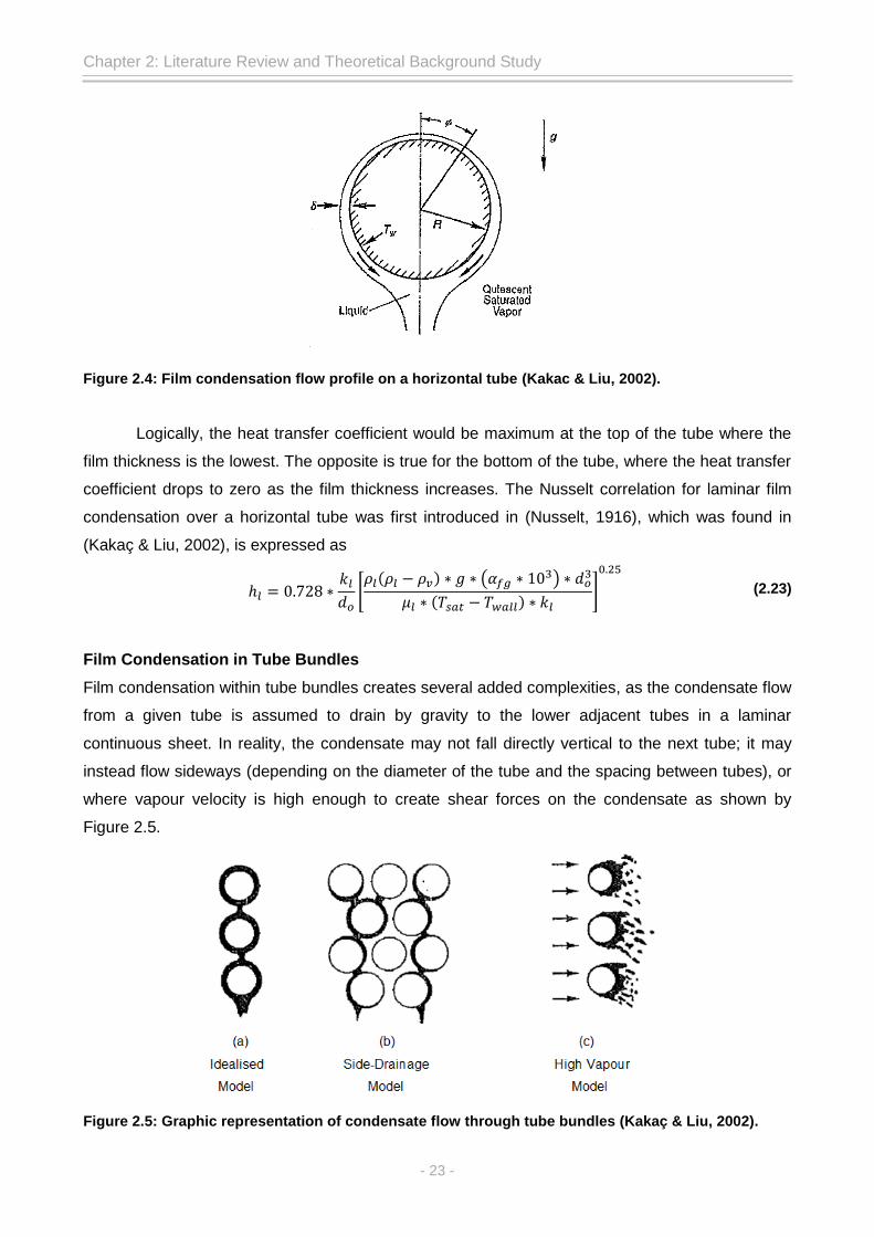
Chapter 2: Literature Review and Theoretical Background Study
- 23 -
Figure 2.4: Film condensation flow profile on a horizontal tube (Kakac & Liu, 2002).
Logically, the heat transfer coefficient would be maximum at the top of the tube where the
film thickness is the lowest. The opposite is true for the bottom of the tube, where the heat transfer
coefficient drops to zero as the film thickness increases. The Nusselt correlation for laminar film
condensation over a horizontal tube was first introduced in (Nusselt, 1916), which was found in
(Kakaç & Liu, 2002), is expressed as
[ ( ) ( )
( ) ]
(2.23)
Film Condensation in Tube Bundles
Film condensation within tube bundles creates several added complexities, as the condensate flow
from a given tube is assumed to drain by gravity to the lower adjacent tubes in a laminar
continuous sheet. In reality, the condensate may not fall directly vertical to the next tube; it may
instead flow sideways (depending on the diameter of the tube and the spacing between tubes), or
where vapour velocity is high enough to create shear forces on the condensate as shown by
Figure 2.5.
Figure 2.5: Graphic representation of condensate flow through tube bundles (Kakaç & Liu, 2002).

Chapter 2: Literature Review and Theoretical Background Study
- 24 -
Where there is an absence of vapour velocity the condensate flow by gravity to the lower
tubes in the tube bundle (known as condensate inundation), then the film thickness around the
lower tubes of the tube bundle should increase and the heat transfer coefficient should decrease
(Wolverine Tube Inc, 2014).
Nusselt (1916) added to his film condensation analysis over a single horizontal tube, by
introducing an idealised in-line tube column model. Nusselt assumed that the condensate from any
given tube in the idealised model would drain to the next tube in a continuous laminar sheet, and
that the (Tsat – Twall) remains constant across all tubes. With these assumptions Nusselt proposed
the average heat transfer coefficient for a vertical column of N tubes, which compares to the top
tube of the column as calculated with Eq. 2.23.
⁄ (2.24)
According to (Kakaç & Liu, 2002), Nusselt also proposed a correlation for the local coefficient at
the Nth tube as
⁄ ( ) ⁄ (2.25)
Kern (1958), as referenced by (Kakaç & Liu, 2002), proposed a less conservative correlation for
the mean and local film condensation heat transfer coefficients as
⁄ (2.26)
and
⁄ ( ) (2.27)
However, the data of numerous experimental measurements have been very scattered and
still today there is no successful theoretical model. Thus, for the purposes of design-sizing and
rating it’s recommended by (Butterworth, 1977) that Eq. 2.26 and Eq. 2.27 are conservative to use
for shell side heat transfer coefficient calculation, when there is an absence of vapour velocity. In
cases where high vapour velocity is present, the condensate is subjected to vapour shear, as
illustrated in Figure 2.5(c). Initially, the effects of vapour shear and condensate inundation where
treated separately. However, according to (Kakaç & Liu, 2002), Butterworth proposed an
inundation and vapour shear local heat transfer coefficient relationship for the Nth tube row in
(Butterworth, 1977) as
[
(
)
]
[
( )
] (2.28)
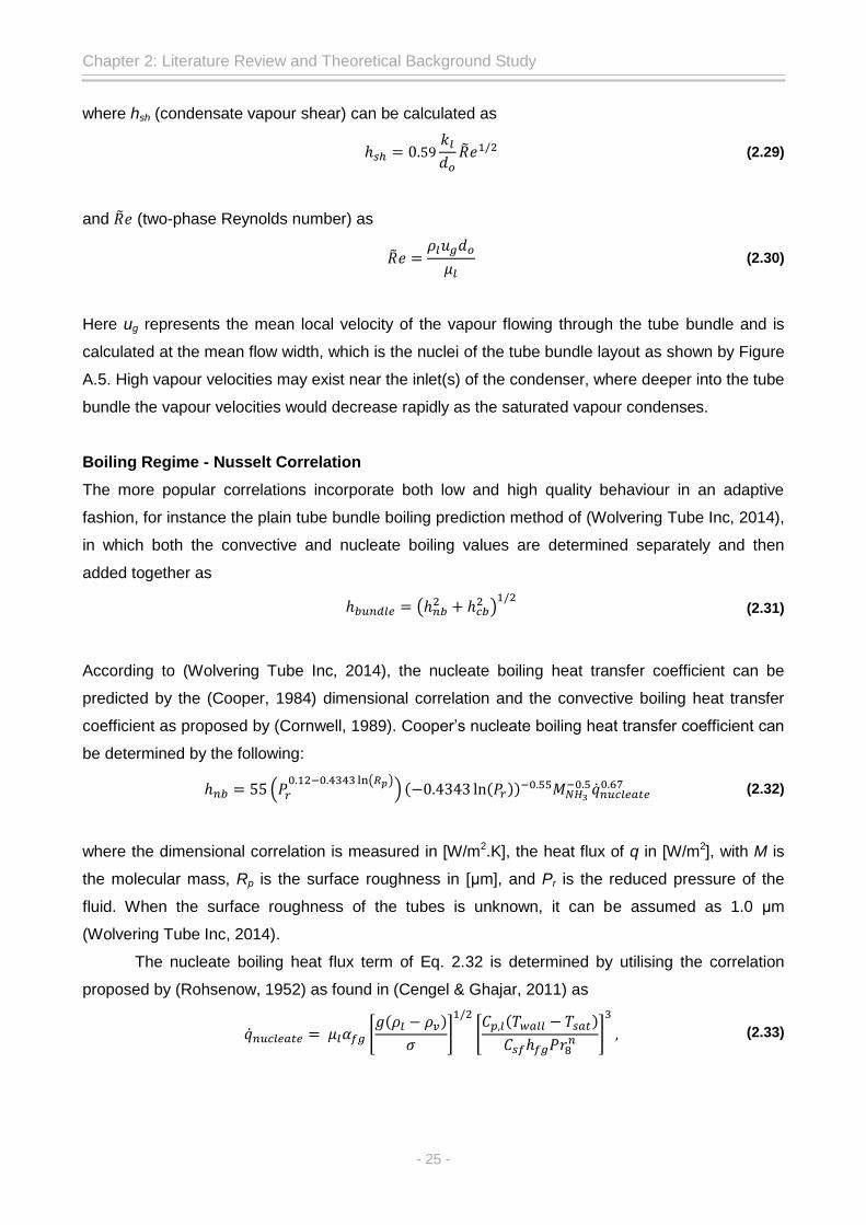
Chapter 2: Literature Review and Theoretical Background Study
- 25 -
where hsh (condensate vapour shear) can be calculated as
(2.29)
and (two-phase Reynolds number) as
(2.30)
Here ug represents the mean local velocity of the vapour flowing through the tube bundle and is
calculated at the mean flow width, which is the nuclei of the tube bundle layout as shown by Figure
A.5. High vapour velocities may exist near the inlet(s) of the condenser, where deeper into the tube
bundle the vapour velocities would decrease rapidly as the saturated vapour condenses.
Boiling Regime - Nusselt Correlation
The more popular correlations incorporate both low and high quality behaviour in an adaptive
fashion, for instance the plain tube bundle boiling prediction method of (Wolvering Tube Inc, 2014),
in which both the convective and nucleate boiling values are determined separately and then
added together as
(
)
(2.31)
According to (Wolvering Tube Inc, 2014), the nucleate boiling heat transfer coefficient can be
predicted by the (Cooper, 1984) dimensional correlation and the convective boiling heat transfer
coefficient as proposed by (Cornwell, 1989). Cooper’s nucleate boiling heat transfer coefficient can
be determined by the following:
( ( )) ( ( ))
(2.32)
where the dimensional correlation is measured in [W/m2.K], the heat flux of q in [W/m2], with M is
the molecular mass, Rp is the surface roughness in [μm], and Pr is the reduced pressure of the
fluid. When the surface roughness of the tubes is unknown, it can be assumed as 1.0 μm
(Wolvering Tube Inc, 2014).
The nucleate boiling heat flux term of Eq. 2.32 is determined by utilising the correlation
proposed by (Rohsenow, 1952) as found in (Cengel & Ghajar, 2011) as
[
( )
]
[ ( )
]
(2.33)
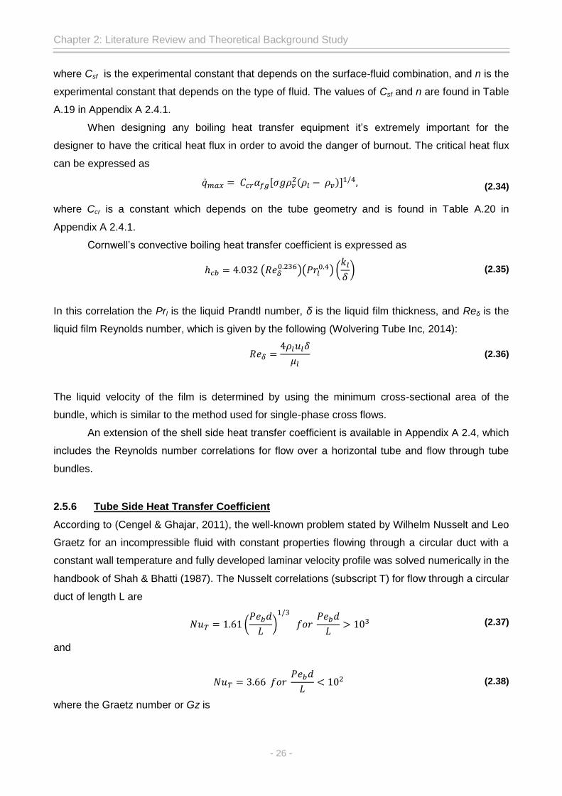
Chapter 2: Literature Review and Theoretical Background Study
- 26 -
where Csf is the experimental constant that depends on the surface-fluid combination, and n is the
experimental constant that depends on the type of fluid. The values of Csf and n are found in Table
A.19 in Appendix A 2.4.1.
When designing any boiling heat transfer equipment it’s extremely important for the
designer to have the critical heat flux in order to avoid the danger of burnout. The critical heat flux
can be expressed as
[ ( )]
(2.34)
where Ccr is a constant which depends on the tube geometry and is found in Table A.20 in
Appendix A 2.4.1.
Cornwell’s convective boiling heat transfer coefficient is expressed as
(
)( ) (
) (2.35)
In this correlation the Prl is the liquid Prandtl number, δ is the liquid film thickness, and Reδ is the
liquid film Reynolds number, which is given by the following (Wolvering Tube Inc, 2014):
(2.36)
The liquid velocity of the film is determined by using the minimum cross-sectional area of the
bundle, which is similar to the method used for single-phase cross flows.
An extension of the shell side heat transfer coefficient is available in Appendix A 2.4, which
includes the Reynolds number correlations for flow over a horizontal tube and flow through tube
bundles.
2.5.6 Tube Side Heat Transfer Coefficient
According to (Cengel & Ghajar, 2011), the well-known problem stated by Wilhelm Nusselt and Leo
Graetz for an incompressible fluid with constant properties flowing through a circular duct with a
constant wall temperature and fully developed laminar velocity profile was solved numerically in the
handbook of Shah & Bhatti (1987). The Nusselt correlations (subscript T) for flow through a circular
duct of length L are
(
)
(2.37)
and
(2.38)
where the Graetz number or Gz is

Chapter 2: Literature Review and Theoretical Background Study
- 27 -
(2.39)
The superposition mean Nusselt number correlation for laminar flow in circular ducts was found in
(Kakaç & Liu, 2002), but originally proposed by (Gnielinski, 1983) to give sufficiently good values
for most practical applications.
[ (
)]
(2.40)
Hausen – Nusselt Correlation for Laminar Flow through Circular Ducts
The empirical Nusselt correlation was originally proposed in (Hausen, 1959) as found in (Kakaç &
Liu, 2002) and (Thulukakanam, 2000), for laminar flow in the thermal entrance region of a circular
duct is comparable to the values of the correlation proposed in Eq. 2.40. The Hausen (1959)
Nusselt correlation is
(
)
(
) (2.41)
The results of Eq. 2.40 and Eq. 2.41 are comparable according to (Kakaç & Liu, 2002), where both
equations can be used for liquids and gases in the range of (0.1 < Pebd/L <104). The Pèclet
number (Peb) is the Reynolds number multiplied with the bulk fluid Prandtl number.
Gnielinski – Nusselt Correlation for Transitional Flow through Circular Ducts
(Gnielinski, 1976) found in (Thulukakanam, 2000) proposed a modified Petukhov-Kirillov Nusselt
correlation of turbulent flow through circular ducts to be applicable to the transitional region of
Reynolds numbers between 2300 and 104:
(
) ( )
(
) ⁄
( ⁄ )
(2.42)
where the friction factor is expressed as
( ) (2.43)
The thermophysical properties of the tube side heat transfer coefficient equations are evaluated at
the bulk fluid temperature of Tbulk, defined as
(2.44)

Chapter 2: Literature Review and Theoretical Background Study
- 28 -
An extension of the tube side heat transfer coefficient is available in Appendix A 2.5, which
includes the Reynolds number correlations for flow though circular ducts.
2.5.7 Heat Transfer Surface Area
The thermodynamic design cannot be completed without the rearranging of Eq. 2.6, which gives
the per tube length of heat transfer surface area as
( ) (2.45)
where all the terms of Eq. 2.45 are known, except for the number of tubes, Nt.
Other physical design dimensions such as the shell diameter Ds, and inner- and outer
diameter of the tubes can be approached as variable input parameters creating multiple design
permutations. These variable input parameters can be standardised sizes of shells and tubes. The
number of tubes in a shell and tube heat exchanger depend on the tube bundle layout, number of
tube passes, Np, the pitch ratio, PR, the shell inner diameter, Ds, and the tube’s outer diameter, do.
The number of tubes can be determined by using the following (Kakaç & Liu, 2002):
(
)(
) (2.46)
where CTP is the number tube pass calculation constant that accounts for the incomplete
coverage of the tubes in the shell, as recorded parameters in Table 2.4. CL is the tube bundle
layout constant, with its parameters recorded in Table 2.5.
Table 2.4: Tube pass constant (Kakaç & Liu, 2002).
One Tube Pass CTP = 0.93
Two Tube Passes CTP = 0.90
Three Tube Passes CTP = 0.85
Table 2.5: Tube bundle layout constant (Kakaç & Liu, 2002).
45° and 90° CL = 1.0
30° and 60° CL = 0.87
2.6 Extended Theoretical Background and Literature Review
The theoretical background of the shell and tube side pressure drop ratings have been excluded
from the main body of this oeuvre, but is available in Appendix A 2.6 & 2.7, respectively. The
equations to determine the fouling overall heat transfer coefficient and percentage over design are
added to Appendix A 2.8. Furthermore, the mechanical design considerations and rating is

Chapter 2: Literature Review and Theoretical Background Study
- 29 -
excluded from the main body of text, as it isn’t the main focus of the study but does play a
fundamental role in the process of heat exchanger designing. The literature review of the
mechanical design rating and considerations are available in Appendix A 3, which depict the stress
calculations of the pressurised shell, tube bundle sheet, and the number of bolts required for each
header. Available in Appendix A 4 is a short literature review of the occupational health and safety
of an aqua-ammonia absorption-desorption H&R cycle.
2.7 Conclusion
In conclusion, the literature review and theoretical background study illustrated the methods of
obtaining conservative thermophysical properties, which are essential in determining the
thermodynamic design and rating model for each of the heat exchangers. The Conde-Petit (2004)
& (2011) mathematical models for determining thermophysical properties have shown to be in
good accordance with similar properties obtained with EES, and are therefore considered
satisfactory for further thermodynamic design purposes. Furthermore, the chapter illustrated the
required shell and tube side heat transfer coefficients correlations required to complete the
thermodynamic design of the aqua-ammonia heat exchangers. An extension to the theoretical
background and literature review was created to keep the main focus of the chapter to the
fundamentals of this study. The following chapter deals with the explanation of how the
thermophysical properties are calculated combined with an investigation into the two-phase region
of aqua-ammonia.

- 30 -
Chapter 3
3 THERMOPHYSICAL PROPERTIES AND THERMODYNAMIC DESIGN SELECTION
Introduction
Chapter 3 focuses on the development of the thermodynamic design selection by investigating
each specific heat exchanger’s inlet and outlet conditions, be it for aqua-ammonia or ethylene
glycol water mixtures. Compiled within Chapter 3 is an in depth investigation into the
thermophysical properties of the two-phase and superheated vapour regions of the theoretical
maximum mass concentration aqua-ammonia solution, and the conclusions drawn from any
anomalies which may occur. The research into the thermophysical properties of 99 wt% aqua-
ammonia carries great effect on what the thermodynamic design output will be for each specific
heat exchanger. Furthermore, an extension of Chapter 3 is adopted in Appendix C, which deals
with the design requirements and the concept generation and evaluation.

Chapter 3: Thermophysical Properties and Thermodynamic Design Selection
- 31 -
3.1 Thermophysical Properties for Aqua-Ammonia Solutions
Figures 3.1 and 3.2 depict the temperature vs. enthalpy of the 99 wt% ammonia refrigerant line
and its thermodynamic states, and the weak and strong aqua-ammonia solutions, respectively.
Together with Fig. 1.3, these figures will serve as a reference for the subsequent sections of this
oeuvre, but remain open to modification and optimisation.
Figure 3.1: Aqua-ammonia absorption-desorption heating and refrigeration heat exchangers temperature vs. enthalpy diagram.
The pressure line of 99 wt% aqua-ammonia is set to a mean system pressure of 7 [bar] and
starts off at point 3. Points 1 and 2 form part of the bubble pump generator and rectifier that is out
of the scope for this study. The temperature of the superheated vapour state 3 was determined as
77.45 [°C] and is then cooled down to the saturated vapour temperature of state 4. The first
anomaly occurs between the latent region of points 4 & 5, as the saturated liquid and vapour
temperature isn’t a constant temperature. This anomaly was defined by Professor John Tomczyk
of Ferris State University as “The temperature difference between the saturated vapour
temperature and the saturated liquid at a constant pressure” (Tomczyk et al., 2016). The
temperature of state 4 is equal to 54.61 [°C] and condenses to saturated liquid at point 5 with
temperature of 15 [°C].
The ‘temperature glide’ of aqua-ammonia causes a slight problem in calculating the heat
transfer coefficient of Eq. 2.48, where Eq. 2.48 requires the use of the saturation temperature,
which in this case isn’t constant. Thus, further investigation is required. Following state 5, the
temperature is lowered by a pre-cool heat exchanger between states 5 to 6. This heat exchanger is
-100 0 100 200 300 400 500 600 700 800 900 1000 1100 1200 1300 1400 1500 1600 1700 1800-20
0
20
40
60
80
100
Enthalpy [kJ/kg]
Te
mp
era
ture
[C
]
3
4
5
6
8 9
10
AmmoniaAqua-Ammonia

Chapter 3: Thermophysical Properties and Thermodynamic Design Selection
- 32 -
added to the cycle to increase the efficiency of the evaporator and thus the COP of the entire
cycle. The sub-cooled liquid of state 6 passes through a venturi to create state 7, whereby the
venturi can be approximated as thermostatic (constant enthalpy). State 7 changes to state 8 as the
liquid is presented to a state of partial pressure, this is due to the tertiary gas (Helium) in the
evaporator module. As the aqueous ammonia feels a partial pressure of 236.2 [kPa] (design
requirement), pure ammonia is able to evaporate instantaneously, to which is known as state 9.
State 9 is heated to state 10 by the pre-cool heat exchanger.
Figure 3.2 illustrates the weak aqua-ammonia solution at 35.92 wt% ammonia and strong
aqua-ammonia solution at 45.3 wt% ammonia at constant pressure of 7 [bar]. Here heat is added
to the strong solution at the cost of heat from the weak solution, also known as regenerative heat
transfer. This is the most important component of the absorption-desorption H&R cycle in terms of
improving the efficiency of the cycle. The cooling of the weak solution liquid line improves the
absorption process, as briefly discussed in Chapter 2.1.7.
Figure 3.2: Weak and strong solutions aqua-ammonia temperature vs. enthalpy diagram.
3.1.1 Aqua-Ammonia Two-Phase Condensation Investigation
Figure 3.3 illustrates the temperature vs. enthalpy curves of three different constant pressures, with
the pressures selected from previous work done by Mr SC van Niekerk as illustrated by the MS
Excel ‘Clear Sky’ data sheet in Appendix D 2.1. The data set obtained from Mr SC van Niekerk
depicted an upper and lower boundary of winter and summer ambient conditions, which have a
direct influence on the bubble pump generator and its aqua-ammonia outlet conditions (system
pressure, temperature, mass flow rate). Therefore, the upper boundary of these conditions were
selected at 5 [°C] and 23 [°C], which herein after be known as winter and summer design
-200 0 200 400 600 800 1000 1200 1400 1600 1800 2000 2200 24000
10
20
30
40
50
60
70
80
90
100
110
120
130
140
150
160
170
180
190
200
Enthalpy [kJ/kg]
Te
mp
era
ture
[C
]
Weak SolutionStrong Solution
ws,in
ws,out
ss,outss,in

Chapter 3: Thermophysical Properties and Thermodynamic Design Selection
- 33 -
conditions, respectively. The third condition selected from the data set is at the average ambient
temperature (15 °C) of Potchefstroom, which herein after be known as the average design
condition.
The temperature versus enthalpy of Fig. 3.3 appears to remain fairly constant after 1200
[kJ/kg], continuing its way down to saturated liquid state. Therefore, marking the ‘turning point’ of
the temperature glide during the condensation process. The graph of Fig. 3.4 better depicts the
turning point of the temperature glide, as it illustrates enthalpy vs. quality of the three design
condition curves.
The conclusions drawn from Fig. 3.4 are simply that the enthalpy remains linear with
relation to quality until it reaches 1200 [kJ/kg], after which enthalpy becomes non-linear. This
change occurs approximately at a quality of 0.94 for each of the three design conditions. Lastly, the
graph of Fig. 3.5 depicts the temperature vs. quality of aqueous ammonia at the three design
conditions. Figure 3.5 clearly indicates the ‘turning point’ of the temperature glide created by an
aqueous ammonia solution, which is approximated at Q = 0.94 as well. The ‘turning point’
temperature is approximated to be in the region of 5 [°C] above the saturated liquid temperature for
all the ambient conditions. Therefore, it’s assumed that state 4 to 5 can be separated into two
sections, namely, state 4 to state TP (Turning Point), and state TP to state 5. The thermodynamic
design selection would be an engineering decision as to whether: a choice of 2 condensing heat
exchangers; or 1 condensing heat exchanger using superposition between states 4 to TP and TP
to 5 are designed for.
Figure 3.3: Temperature vs. enthalpy of state 3 to 5 for three ambient design conditions.
0 100 200 300 400 500 600 700 800 900 1000 1100 1200 1300 1400 1500 1600 1700
0
10
20
30
40
50
60
70
80
90
100
Enthalpy [kJ/kg]
Tem
pera
ture
[C
]
939.54 kPa
727.25 kPa
515.84 kPa5 [C]
15 [C]
23 [C]5
5
5
95.36 [C]3
77.5 [C]3
64.2 [C]4
58.2[C]455.4 [C]
50.4 [C]4
3

Chapter 3: Thermophysical Properties and Thermodynamic Design Selection
- 34 -
Figure 3.4: Enthalpy vs. quality of the two-phase region for three ambient design conditions of aqua-ammonia.
Figure 3.5: Temperature vs. quality of the two-phase region for three ambient design conditions of aqua-ammonia.
-0.05 0.05 0.15 0.25 0.35 0.45 0.55 0.65 0.75 0.85 0.95 1.05
0
200
400
600
800
1000
1200
1400
Quality [-]
En
thalp
y [
kJ/k
g] 939.54 kPa
727.25 kPa
515.84 kPa
Q = 0.94
1200 kJ/kg
-0.1 0 0.1 0.2 0.3 0.4 0.5 0.6 0.7 0.8 0.9 1 1.1
0
10
20
30
40
50
60
70
80
90
100
110
Quality [-]
Tem
pera
ture
[C
]
Q = 0.94
939.54 kPa
727.25 kPa
515.84 kPa
28 [C]
20 [C]
15 [C]

Chapter 3: Thermophysical Properties and Thermodynamic Design Selection
- 35 -
Enthalpy of State TP
The enthalpy of state TP at Qx,TP = 0.94 can be approximated as a linear function of quality, as
depicted by Fig. 3.6. The black line represents the actual curve of enthalpy as a function of quality,
where the red line represents the enthalpy as a linear function of quality. The linear enthalpy
approximation is derived by using the grey (dash-dot) construction lines.
Figure 3.6: Linear enthalpy vs. quality estimation of aqua-ammonia in the two-phase region and the graphical representation of the ‘turning point’.
-0.05 0.05 0.15 0.25 0.35 0.45 0.55 0.65 0.75 0.85 0.95 1.050
100
200
300
400
500
600
700
800
900
1000
1100
1200
1300
1400
1500
Quality [-]
En
thalp
y [
kJ/k
g]
Qest = 0.1
Q = 0.94
Enthalpyest
0.85 0.875 0.9 0.925 0.95 0.975 1 1.025 1.05900
950
1000
1050
1100
1150
1200
1250
1300
1350
1400
1450
1500
Quality [-]
En
thalp
y [
kJ/k
g]
Q = 0.94Qest = 0.1
Enthalpyest
Q = 1.00
TP
1
2
3
4
5

Chapter 3: Thermophysical Properties and Thermodynamic Design Selection
- 36 -
The first construction line to be drawn is from saturated liquid straight to saturated vapour
(line numbered; 1), secondly the dotted line under the actual curve is drawn towards the saturated
vapour vertical line (line numbered; 2). After which a horizontal line is placed at the intersection of
the dotted line and the vertical saturated vapour line (line numbered; 3), this forms the enthalpy
estimation if the enthalpy of aqua-ammonia had a linear temperature glide. The horizontal enthalpy
estimation line creates an intersection of line number 1 (line numbered; 4), thus creating the quality
estimation from the saturated vapour side. Lastly, the intersecting lines of Qx,TP = 0.94 and line
number 3 are connected to saturated vapour of the actual enthalpy curve (line numbered 5) to form
the new linear estimation of enthalpy.
This process was completed for the average design conditions (727.25 kPa), so that a
unified method could be applied to the remaining two conditions. The equations for enthalpy
estimation and enthalpy of state TP are derived from a linear weighted function of quality and are
expressed as:
(( ) ) (3.1)
and
( ) (3.2)
3.1.2 Thermophysical Properties of State 3 to 5
This section focuses on state 3, 4, TP, and 5 of Figure 3.1, with respect to each state’s
thermophysical properties and what impact it will have on the design selection of each heat
exchanger. The thermodynamic design was completed for all three ambient design conditions to
confirm which of these conditions yielded the ‘worst case’ scenario. The ‘worst case’ is viewed as
the condition that demands the largest heat transfer surface area. A trend appeared as to which
condition normally yields the ‘worst case’ scenario, which is a combination of the highest heat
transfer rate between states and the refrigerant mass flow rate. Thus, an energy balance is
required to determine the ‘worst case’ scenario between each of the states and their respective
mass flow rates as prescribed by Eq. 2.1.
Enthalpy of State 3 through 5
The enthalpy of the superheated vapour state 3 can be obtained as a conservative value by means
of EES’ built-in property function. As documented by Table A.7, the enthalpy values for saturated
liquid and vapour are within good accordance between the mathematical method and EES. Thus,
for purposes of consistency the mathematical method will be used for all thermophysical properties
within the two-phase region. Enthalpy of state 3 is determined with EES’ property function;

Chapter 3: Thermophysical Properties and Thermodynamic Design Selection
- 37 -
enthalpy of state 4 is calculated by using Eq. A.3; the enthalpy of state 5 is calculated using Eq.
A.2; and lastly the enthalpy of state TP is calculated using Eq. A.2. Recorded in Table 3.1 are the
enthalpy values of states 3, 4, TP, and 5.
Table 3.1: Enthalpy output values for thermodynamic states 3, 4, TP, & 5.
State Winter
Conditions Average
Conditions Summer
Conditions
3 1409 [kJ/kg] 1453 [kJ/kg] 1489 [kJ/kg]
4 1384.169 [kJ/kg] 1391.113 [kJ/kg] 1395.661 [kJ/kg]
TP 1182.205 [kJ/kg] 1235.08 [kJ/kg] 1277.245 [kJ/kg]
5 11.197 [kJ/kg] 58.198 [kJ/kg] 96.515 [kJ/kg]
Now that the enthalpy values of state 3 through 5 have been calculated, it’s possible to determine
the heat transfer rate of each control volume.
Control volume for state 3 to 4:
Winter design conditions:
Average design conditions:
Summer design conditions:
Thus, for state 3 to 4, it is clear that under summer conditions the heat transfer rate is the highest.
In this oeuvre, the summer condition thermophysical properties of state 3 will be illustrated within
the main document, where the thermophysical properties of the remaining design conditions are
added to Appendix B 2.
��𝑊𝑅𝑇 �� 𝑊𝑅𝑇(𝛼 𝑊𝑅𝑇 𝛼 𝑊𝑅𝑇) (𝐸𝑞 )
∴ ( )
∴ 𝑊 (𝐻𝑒𝑎𝑡 𝑅𝑒𝑚𝑜𝑣𝑒𝑑)
��𝐷𝑆𝑁 �� 𝐷𝑆𝑁(𝛼 𝐷𝑆𝑁 𝛼 𝐷𝑆𝑁) (𝐸𝑞 )
∴ ( )
∴ 𝑊 (𝐻𝑒𝑎𝑡 𝑅𝑒𝑚𝑜𝑣𝑒𝑑)
��𝑆𝑀𝑅 �� 𝑆𝑀𝑅(𝛼 𝑆𝑀𝑅 𝛼 𝑆𝑀𝑅) (𝐸𝑞 )
∴ ( )
∴ 𝑊 (𝐻𝑒𝑎𝑡 𝑅𝑒𝑚𝑜𝑣𝑒𝑑)

Chapter 3: Thermophysical Properties and Thermodynamic Design Selection
- 38 -
The control volume for State 4 to 5 is
Superposition will be used to determine the highest heat transfer rate of the condenser control
volume, as it better represents the enthalpy curve as illustrated in Fig. 3.3.
Winter design conditions 4 to TP:
Average design conditions 4 to TP:
Summer design conditions 4 to TP:
Winter design conditions TP to 5:
Average design conditions TP to 5:
Summer design conditions TP to 5:
With the total heat transfer rate of each condition adding up to:
Winter Conditions = 743.052 W (Heat Removed)
Average Conditions = 778.289 W (Heat Removed)
Summer Conditions = 799.365 W (Heat Removed)
The thermophysical properties of summer conditions for state 4, TP, and 5 will be illustrated with
sample calculations within the main body of the dissertation. The thermophysical properties of
remaining states of the absorption-desorption cycle will be tabulated, with sample calculations
added to Appendix B.
��𝑊𝑅𝑇 �� 𝑊𝑅𝑇(𝛼𝑇𝑃 𝑊𝑅𝑇 𝛼 𝑊𝑅𝑇) (𝐸𝑞 )
∴ ( )
∴ 𝑊 (𝐻𝑒𝑎𝑡 𝑅𝑒𝑚𝑜𝑣𝑒𝑑)
��𝐷𝑆𝑁 �� 𝐷𝑆𝑁(𝛼𝑇𝑃 𝐷𝑆𝑁 𝛼 𝐷𝑆𝑁) (𝐸𝑞 )
∴ ( )
∴ 𝑊 (𝐻𝑒𝑎𝑡 𝑅𝑒𝑚𝑜𝑣𝑒𝑑)
��𝑆𝑀𝑅 �� 𝑆𝑀𝑅(𝛼𝑇𝑃 𝑆𝑀𝑅 𝛼 𝑆𝑀𝑅) (𝐸𝑞 )
∴ ( )
∴ 𝑊 (𝐻𝑒𝑎𝑡 𝑅𝑒𝑚𝑜𝑣𝑒𝑑)
��𝑊𝑅𝑇 �� 𝑊𝑅𝑇(𝛼 𝑊𝑅𝑇 𝛼𝑇𝑃 𝑊𝑅𝑇) (𝐸𝑞 )
∴ ( )
∴ 𝑊 (𝐻𝑒𝑎𝑡 𝑅𝑒𝑚𝑜𝑣𝑒𝑑)
��𝐷𝑆𝑁 �� 𝐷𝑆𝑁(𝛼 𝐷𝑆𝑁 𝛼𝑇𝑃 𝐷𝑆𝑁) (𝐸𝑞 )
∴ ( )
∴ 𝑊 (𝐻𝑒𝑎𝑡 𝑅𝑒𝑚𝑜𝑣𝑒𝑑)
��𝑆𝑀𝑅 �� 𝑆𝑀𝑅(𝛼 𝑆𝑀𝑅 𝛼𝑇𝑃 𝑆𝑀𝑅) (𝐸𝑞 )
∴ ( )
∴ 𝑊 (𝐻𝑒𝑎𝑡 𝑅𝑒𝑚𝑜𝑣𝑒𝑑)

Chapter 3: Thermophysical Properties and Thermodynamic Design Selection
- 39 -
State 3 Thermophysical Properties
The superheated vapour phase of state 3 proved cumbersome, whereby neither EES’ built-in
property functions nor (Conde-Petit, 2004) formulae could provide accurate thermophysical
properties. It was decided as a conservative approach to determine the thermophysical properties
of state 3 as linearly weighted properties with pure ammonia and water at their respective
temperatures and ambient design condition pressures. However, it’s well known that properties do
not necessarily behave linearly in the superheated region, but the thermophysical properties of
enthalpy and density can be approximated as linear functions. The temperatures of the pure
substances are calculated by using Eqs. A.1 and A.7 for the aqua-ammonia vapour solution
temperature.
The Engineering Equation Solver does however provide a conservative value for density in
the superheated region of aqueous ammonia. Table 3.2 represents the thermophysical properties
of pure ammonia and water at summer design condition pressure, and recorded in Table 3.3 is the
linearly weighted thermophysical properties of state 3 at the pre-determined ‘worst case’ of
summer conditions. The transport properties of aqua-ammonia were obtained by using EES’ built-
in property functions and a linearly weighted property equation according to the mass
concentration of aqueous ammonia, which is simply expressed as
( ) (3.3)
The specific thermal capacity is determined with an energy balance using Eqs. 2.1 and 2.2.
The values of dynamic viscosity, thermal conductivity, and Prandtl number are determined as
stated above with Eq. 3.3.
Table 3.2: Thermophysical properties of pure ammonia and water for state 3.
Thermophysical Properties (Summer Conditions)
T3,NH3 92.2348 °C
T3,H2O 310.114 °C
P3,NH3 939.54 kPa P3,H2O 939.54 kPa
α3,NH3 1665 kJ/kg α3,H2O 2216 kJ/kg
Cp3,NH3 2.462 kJ/kg.K Cp3,H2O 2.701 kJ/kg.K
ρ3,NH3 5.522 kg/m3 ρ3,H2O 3.326 kg/m3
µ3,NH3 0.00001255 kg/m.s µ3,H2O 0.00002108 kg/m.s
k3,NH3 0.03325 W/m.K k3,H2O 0.06675 W/m.K
Pr3,NH3 0.9293 Pr3,H2O 0.8529

Chapter 3: Thermophysical Properties and Thermodynamic Design Selection
- 40 -
Table 3.3: Thermophysical properties of aqua-ammonia for state 3.
LINEAR WEIGHTED PROPERTIES
α3 1489 kJ/kg
Cp3 1.1443 kJ/kg.K
ρ3 5.48 kg/m3
µ3 1.264E-05 kg/m.s
k3 0.033585 W/m.K
Pr3 0.928536
State 4 Thermophysical Properties
The saturated vapour properties of state 4 will be calculated by using the mathematical model set
out in Appendix A 1.1 for saturated aqua-ammonia vapour. These properties are calculated for
summer design conditions, as illustrated by the ‘worst case’ scenario calculations of states 3 to 4,
and 4 to 5. The mathematical method requires several input parameters of which are:
Pressure
Mass concentration
Molar vapour concentration
The saturated vapour aqua-ammonia mixture temperature is calculated using Eq. A.1 by
substituting for summer condition pressure (939.54 kPa) and ammonia mass concentration (0.99).
The molar vapour concentration is determined by using Eq. A.4 and substituting for summer
condition pressure (939.54 kPa) and ammonia mass concentration (0.99).
Recorded in the box below are the thermophysical properties of saturated aqua-ammonia vapour,
of which the sample calculations are available in Appendix B 1.1.
𝑇 ( ) [𝐾]𝑜𝑟 [ 𝐶]
𝑦( ) [ ]
𝐶𝑝 [𝑘𝐽
𝑘𝑔]
𝜌 [𝑘𝑔
𝑚 ]
𝜇 𝐸( ) [𝑘𝑔
𝑚 𝑠]
𝑘 [𝑊
𝑚 𝐾]
𝑃𝑟 [ ]

Chapter 3: Thermophysical Properties and Thermodynamic Design Selection
- 41 -
State 5 Thermophysical Properties
The saturated liquid properties of state 4 will be calculated by using the mathematical method set
out in Appendix A 1.1 for saturated aqua-ammonia liquid. These properties are calculated for
summer design conditions, as illustrated by the ‘worst case’ scenario calculations of states 3 to 4,
and 4 to 5.
The mathematical method requires two input parameters of which are:
Pressure
Mass concentration
With these input parameters the temperature of the 99 wt% aqua-ammonia mixture can be
calculated by using Eq. A.1 and its supporting equation parameters in Table A.2.
The thermophysical properties of saturated aqua-ammonia liquid are presented by the following:
The sample calculations of the mathematical model proposed by Conde-Petit (2004) are available
in Appendix B 1.2.
State TP (Turning Point) Thermophysical Properties
The thermophysical properties of state TP has proved to be vague, as state TP falls within the two-
phase state of aqua-ammonia. Very few articles exist explaining the characteristics of the two-
phase region for aqua-ammonia. As previously iterated, EES does provide a conservative value for
the density of aqueous ammonia. Thus, by using EES’ built-in property call function for density a
graph can be plotted as a function of quality, as illustrated in Fig. 3.7.
𝑇( ) [𝐾]𝑜𝑟 [ 𝐶]
𝐶𝑝 [𝑘𝐽
𝑘𝑔]
𝜌 [𝑘𝑔
𝑚 ]
𝜇 [𝑘𝑔
𝑚 𝑠]
𝑘 [𝑊
𝑚 𝐾]
𝑃𝑟 [ ]

Chapter 3: Thermophysical Properties and Thermodynamic Design Selection
- 42 -
Figure 3.7: Density vs. quality for aqua-ammonia in the two-phase region of three ambient design conditions.
The black line represents the quality at which state TP occurs (Q = 0.94); the orange curve
represents the density of 99 wt% aqua-ammonia at 7 [bar] as a function of quality. The linear
approximation is made by using the grey construction lines. The first construction line to be drawn
is to connect saturated liquid to saturated vapour (line numbered; 1), secondly the line following the
density curve (line numbered; 2). The third construction line represent what the density would be if
-0.05 0.05 0.15 0.25 0.35 0.45 0.55 0.65 0.75 0.85 0.95 1.050
100
200
300
400
500
600
700
Quality [-]
Den
sit
y [
kg
/m3]
939.54 kPa
727.25 kPa
515.84 kPa
Q = 0.94
1
2
3
-0.05 0.05 0.15 0.25 0.35 0.45 0.55 0.65 0.75 0.85 0.95 1.050
20
40
60
80
100
Quality [-]
Den
sit
y [
kg
/m3]
Q = 0.94
Density Estimation at State TP
1
2
3

Chapter 3: Thermophysical Properties and Thermodynamic Design Selection
- 43 -
a point to point linear correlation is made. The density of state TP, would typically be approximated
by a simple linear weighted equation, as expressed by the following equation:
(( ) ( )) (3.4)
Although, as illustrated by the construction lines of Figure 3.7, the density of state TP can be
approximated by
(( ) ) (3.5)
With this method the density is approximated from the saturated vapour value, and because the
quality of the turning point is close to Q = 1.00 the approximated value of density is much closer to
its actual density at Q = 0.94. The density of state TP for summer conditions can be calculated as
The remaining properties of dynamic viscosity, thermal conductivity, and Prandtl number
have little known two-phase characteristics, or graph interpreting the two-phase region. Thus, as a
conservative approach the thermophysical properties are approximated with a point to point linear
approximation.
(( ) ( )) (3.6)
The dynamic viscosity can be calculated as
The thermal conductivity is approximated as
The Prandtl number can be approximated using Eq. A.25, but as the specific thermal
capacity is needed and the two-phase specific thermal capacity curve is not known, thus the
Prandtl number is calculated using Eq. 3.6.
𝜌𝑇𝑃 𝜌 (( 𝑄𝑥 𝑇𝑃) 𝜌 ) (𝐸𝑞 )
∴ (( ) )
∴ [𝑘𝑔
𝑚 ]
𝜇𝑇𝑃 𝜇 ((𝜇 𝜇 ) ( 𝑄𝑥 𝑇𝑃))
∴ 𝐸( ) (( 𝐸( ) ) ( ))
∴ 𝐸( ) [𝑘𝑔
𝑚 𝑠]
𝑘𝑇𝑃 𝑘 ((𝑘 𝑘 ) ( 𝑄𝑥 𝑇𝑃))
∴ (( ) ( ))
∴ [𝑊
𝑚 𝐾]

Chapter 3: Thermophysical Properties and Thermodynamic Design Selection
- 44 -
Note: The sample calculations of the thermophysical properties of states 5 to 6 and 9 to 10 are available in
Appendix B 1.3, as the method of determining the thermophysical properties can be considered trivial.
3.1.3 Thermophysical Properties of State 7 to 8
The sub-cooled liquid of state 6 flows through a venturi nozzle into the evaporator module,
whereby the venturi nozzle is isothermal and the sub-cooled liquid would enter the two-phase
region with the drop in pressure, now, known as state 7. Added to the drop in pressure, the two-
phase liquid feels partial pressure due to Helium in the evaporator module, thus creating state 8. It
is assumed that from state 7 to 8 remains isothermal and the quality of two-phase fluid can be
determined by a similar but modified method used for the turning point state.
Figure 3.8 depicts the enthalpy curve of 99 wt% aqua-ammonia and pressure of 236.39
[kPa]. The black line indicates the actual enthalpy curve and the red line depicts the linear enthalpy
estimation. The blue lines indicate the construction lines needed to form the linear enthalpy
estimation. Similar to the turning point, the Qest = 0.1 and the turning point of the curve remains at
Q = 0.94. As the enthalpy of state 8 is known, the linear estimation is used to determine the quality
of state 8.
Figure 3.8: Linear enthalpy estimation of aqua-ammonia at 236.39 [kPa].
0 0.05 0.1 0.15 0.2 0.25 0.3 0.35 0.4 0.45 0.5 0.55 0.6 0.65 0.7 0.75 0.8 0.85 0.9 0.95 1
0
200
400
600
800
1000
1200
1400
1600
Quality [-]
En
thalp
y [
kJ/k
g]
-25.816 [kJ/kg]
Q = 0.94
Qest = 0.1
Qactual
236.39 kPa
Actual Enthalpy Curve
Linear Enthalpy Estimation
TP
𝑃𝑟𝑇𝑃 𝑃𝑟 ((𝑃𝑟 𝑃𝑟 ) ( 𝑄𝑥 𝑇𝑃))
∴ (( ) ( ))
∴ [ ]

Chapter 3: Thermophysical Properties and Thermodynamic Design Selection
- 45 -
The enthalpy of the evaporator can be estimated with the method derived in Eq. 3.1. Now, the
values of saturated liquid and vapour enthalpy (αl = -80.43533 kJ/kg and αg = 1366.0361 kJ/kg as
obtained from the mathematical method) are substituted into Eq. 3.1 and the enthalpy estimation is
calculated as
As state 7 to 8 is a constant enthalpy and has different values for each of the ambient design
conditions, the quality of each condition is thus calculated as
Energy Balance of State 8 to 9
Now, it’s possible to determine the heat transfer rate of the evaporative two-phase line, now that
the enthalpy values of state 8 and 9 are known for all ambient design conditions.
Winter Design Conditions:
𝛼𝑒𝑠𝑡 [𝑘𝐽
𝑘𝑔]
𝑄𝑥 𝑊𝑅𝑇 (𝛼𝑔 𝛼
𝛼𝑔 𝛼𝑒𝑠𝑡)
∴ ( ( )
)
∴
𝑄𝑥 𝐷𝑆𝑁 (𝛼𝑔 𝛼
𝛼𝑔 𝛼𝑒𝑠𝑡)
∴ ( ( )
)
∴
𝑄𝑥 𝑆𝑀𝑅 (𝛼𝑔 𝛼
𝛼𝑔 𝛼𝑒𝑠𝑡)
∴ ( ( )
)
∴
��𝐸𝑉𝐴𝑃 𝑊𝑅𝑇 ��9 𝑊𝑅𝑇(𝛼9 𝑊𝑅𝑇 𝛼 𝑊𝑅𝑇) (𝐸𝑞 )
∴ ( ( ))
∴ 𝑊 (𝐻𝑒𝑎𝑡 𝐴𝑑𝑑𝑒𝑑)

Chapter 3: Thermophysical Properties and Thermodynamic Design Selection
- 46 -
Average Design Conditions:
Summer Design Conditions:
The highest heat transfer is obtained during summer ambient conditions, which is due to the higher
mass flow rate of the refrigerant during summer conditions. Under summer ambient conditions the
evaporator would need a larger heat transfer surface area, as the evaporator would need to
remove more heat from the secondary refrigerant with the warmer ambient conditions.
State 8 Thermophysical Properties
The thermophysical properties of state 8 will be demonstrated for summer design conditions. The
values of specific thermal capacity, dynamic viscosity, thermal conductivity, and Prandtl number
can be calculated by using a point to point linear relation, similar to the process used to determine
the thermophysical properties of state TP with Eq. 3.6.
��𝐸𝑉𝐴𝑃 𝐷𝑆𝑁 ��9 𝐷𝑆𝑁(𝛼9 𝐷𝑆𝑁 𝛼 𝐷𝑆𝑁) (𝐸𝑞 )
∴ ( )
∴ 𝑊 (𝐻𝑒𝑎𝑡 𝐴𝑑𝑑𝑒𝑑)
��𝐸𝑉𝐴𝑃 𝑆𝑀𝑅 ��9 𝑆𝑀𝑅(𝛼9 𝑆𝑀𝑅 𝛼 𝑆𝑀𝑅) (𝐸𝑞 )
∴ ( )
∴ 𝑊 (𝐻𝑒𝑎𝑡 𝐴𝑑𝑑𝑒𝑑)
𝜃 𝜃𝑙 ((𝜃𝑙 𝜃𝑔) ( 𝑄𝑥 𝑆𝑀𝑅)) (𝐸𝑞 )
𝐶𝑝 𝑆𝑀𝑅 (( ) ( ))
∴ [𝑘𝐽
𝑘𝑔 𝐾]
𝜇 𝑆𝑀𝑅 (( 𝐸( )) ( ))
∴ [𝑘𝑔
𝑚 𝑠]
𝑘 𝑆𝑀𝑅 (( ) ( ))
∴ [𝑊
𝑚 𝐾]
𝑃𝑟 𝑆𝑀𝑅 (( ) ( ))
∴ [ ]

Chapter 3: Thermophysical Properties and Thermodynamic Design Selection
- 47 -
3.1.4 Thermophysical Properties of Weak and Strong Aqua-Ammonia Solutions
Figure 3.1 illustrated the regenerative heat exchanger to be between the absorber (absorption) and
bubble pump (desorption) components, and it plays an integral role in the absorption – desorption
H&R cycle. Figure 3.2 illustrated the regenerative heat exchanger cooling the weak solution aqua-
ammonia exiting the bubble pump heading its way to the absorber module, thus, increasing the
efficiency of the absorber by increasing the absorbability of ammonia into the weak solution. In turn
heat is added to the strong solution exiting the absorber heading towards the bubble pump,
increasing the efficiency of the bubble pump by decreasing the heat input needed to boil ammonia
out of the strong solution. Thus for the regenerative heat exchanger, collaboration was required
with the research project responsible for the thermodynamic design of the absorber module. The
weak solution outlet and strong solution inlet parameters of the bubble pump are already known
and can be found on the data sheet labelled ‘Clear Sky’ in Appendix D 8.1.
The temperature of the weak solution entering the absorber was adjusted to the same
temperature of the saturated liquid of state 5, which is equivalent to the ambient temperature.
Although, another heat exchanger is required to lower the temperature of the weak solution to near
ambient temperatures, which hereinafter will be referred to as the auxiliary heat exchanger. Figure
3.9 illustrates temperature vs. enthalpy of the weak and strong solutions to better visualise the
revised processes that the weak and strong solutions will undergo. The numbering of the auxiliary
and regenerative HTEX’s thermodynamic states are changed from in and out to 1, 2, and 3.
The temperature and mass concentration of the strong aqua-ammonia solution could be
determined with the use of the absorber simulation model generated by E van Niekerk. The input
parameters required by the absorber simulation model are: temperatures for the weak aqua-
ammonia solution, state 10, and coolant; mass flow rates of weak solution, state 10, and coolant;
and lastly mass concentration of weak solution.
Figure 3.9: Temperature vs. enthalpy of the auxiliary and regenerative heat exchangers.
-200 0 200 400 600 800 1000 1200 1400 1600 1800 2000 2200 24000
20
40
60
80
100
120
140
160
180
200
Enthalpy [kJ/kg]
Te
mp
era
ture
[C
]
Weak SolutionStrong Solution
ws,1
ws,2ss,2
ss,1
ws,3

Chapter 3: Thermophysical Properties and Thermodynamic Design Selection
- 48 -
The temperatures of the strong aqua-ammonia solution into the regenerative heat exchanger are:
The inlet temperatures of the strong solution confirm the need for an ‘auxiliary’ heat exchanger to
further cool the weak solution liquid line. The quality parameter of the strong solution out of the
regenerative heat exchanger has been pre-determined and is found on the ‘Clear Sky’ data sheet
in Appendix D as
The remainder of the weak and strong aqua-ammonia solutions thermophysical properties
sample calculations are available in Appendix B 1.4. It’s however important to note that the ‘worst
case’ scenario for both heat exchangers is winter ambient conditions, and that for purposes of the
design continuity for the regenerative and auxiliary heat exchangers the thermophysical properties
will be calculated using EES’ thermophysical property call function.
3.1.5 Conclusion of Thermophysical Properties of Aqua-Ammonia Solutions
In conclusion to the thermophysical properties of the aqua-ammonia refrigerant illustrated in
Chapter 3 and Appendix B, is that the mathematical method proposed by (Conde-Petit, 2004) falls
within good accordance to thermophysical properties obtained from EES’ built-in property call
function. The mathematical method of calculating thermophysical properties was primarily
completed using MS Excel as the preliminary thermodynamic design will firstly be completed in MS
Excel. The thermophysical property model coding of MS Excel was verified with no mathematical
errors by coding the same Conde-Petit (2004) mathematical models into EES.
3.2 Extended Chapter 3 – Thermophysical Properties and Thermodynamic Design
Selection
Omitted from Chapter 3 are the thermophysical property calculations of ethylene glycol water
mixtures, which is available in Appendix B 1.5. The reason for the omission of the thermophysical
property calculations is that the subject isn’t fundamental to this study, but does play an important
role in the determination of heat exchanger sizing and rating. Furthermore, the concept design
generation and evaluation is omitted from Chapter 3, but is available in Appendix C. This section is
fairly large and has a very important role in determining a heat exchanger’s configuration, but it
𝑇𝑠𝑠 𝑖𝑛 𝑊𝑅𝑇( ) [ 𝐶]
𝑇𝑠𝑠 𝑖𝑛 𝐷𝑆𝑁( ) [ 𝐶]
𝑇𝑠𝑠 𝑖𝑛 𝑆𝑀𝑅( ) [ 𝐶]
𝑇𝑠𝑠 𝑜𝑢𝑡 𝑊𝑅𝑇( ) [ 𝐶] 𝑤𝑖𝑡 𝑄
𝑇𝑠𝑠 𝑜𝑢𝑡 𝐷𝑆𝑁( ) [ 𝐶] 𝑤𝑖𝑡 𝑄
𝑇𝑠𝑠 𝑜𝑢𝑡 𝑆𝑀𝑅( ) [ 𝐶] 𝑤𝑖𝑡 𝑄

Chapter 3: Thermophysical Properties and Thermodynamic Design Selection
- 49 -
shifts the focus away from the thermodynamic design of a heat exchanger to the physical design of
a heat exchanger. The concepts illustrated in Appendix C are the concepts which passed the early
elimination hurdle, as the oeuvre tries to be concise and to the point those concepts weren’t added
to the final report. The concepts of Appendix C are evaluated with a weighted level of importance
of the specific heat exchanger’s design requirements. Consequently, it’s recommended to read
through Appendix C before continuing onto Chapter 4 to be able to fully comprehend the
thermodynamic design and rating of Chapter 4.
3.3 Conclusion
In conclusion, Chapter 3 has demonstrated all the thermophysical properties and heat exchanger
design selections required to complete the thermodynamic design of Chapter 4. Research to
investigate the two-phase phenomena of aqueous ammonia was completed, and a linear approach
adopted to determine the thermodynamic and transport properties of the two-phase region. The
linear approach created in section 3.1.1 was applied to the evaporator’s two-phase region as well.
Here sub-cooled liquid undergoes a sudden phase change as it passes through the venturi nozzle.
Furthermore, an additional heat exchanger was added to the original control volume cycle layout of
Fig 1.3.

- 50 -
Chapter 4
4 THERMODYNAMIC DESIGN AND RATING
Introduction
Chapter 4 deals with the specific thermodynamic design and rating calculations required for each
of the heat exchangers for an aqua-ammonia absorption-desorption heating & refrigeration unit,
including any alternative components assisting the main heat exchangers. The heat exchanger
design calculations for all of the heat exchanger designs of this oeuvre are completed under the
following set of assumptions:
Steady state operating conditions exist;
The heat exchanger is well insulated so that heat loss to the surroundings is negligible.
The thickness of the tubes is considered negligible since it is thin-walled.
Changes in potential and kinetic energies of the working fluid streams are negligible.
The overall heat transfer coefficient is assumed to be uniform across the length of the heat
exchanger.
Compiled within each heat exchanger’s subsection is the necessary equations and example
calculations to determine the heat exchanger’s size and performance rating. For the completion of
the sizing problem, the log mean temperature difference method was used, with an array of
standardised dimensional parameters for the shell’s inner diameter and the tube’s inner- and outer
diameters. The preliminary design-sizing calculation will first be completed using MS Excel and the
verification thereof will be completed using EES. The performance rating problem will be
completed using the NTU-effectiveness method with MS Excel, after the heat exchanger’s
preliminary design-sizing model is calculated, but before the preliminary design is verified. The
performance rating acts as a benchmark that illustrates whether a heat exchanger is practically
viable and whether the assumed coolant outlet temperature is within a practically expected range.

Chapter 4: Thermodynamic Design and Rating
- 51 -
4.1 Overview of the Experimental Setup
The heat exchangers of the solar powered aqua-ammonia absorption-desorption heating and
refrigeration package unit is required to fit within a structural housing, with dimensions illustrated in
Fig. 4.1. The heat storage setup and the heat sink setup must be stored within the structural
housing and the solar collector setup on the outside of the structure. The solar collector has a
downstream effect on the absorption-desorption cycle, as it provides the cycle with its heat source.
The heat sink setup will directly influence the heat exchangers of the absorption-desorption cycle,
as it will house and distribute the ethylene glycol-water solution throughout the most of the cycle
(see Fig. 4.2 for coolant flow visualisation).
Figure 4.1: Schematic representation of the housing structure for the solar-driven aqua-ammonia absorption-desorption heating & refrigeration package unit.
Although the dimensional parameter that the housing structure creates is 1.5x3.6x1.8, it
cannot be used as the dimensional design parameter for each of the heat exchanger designs.
Therefore, the cubic size parameter of each heat exchanger is limited to length < 2.5 [m], width < 1
[m], and height < 1 [m]. The housing structure is specified to be able to withstand a load of 750 [kg]
suspended from its ceiling, therefore the suspended stage 1 & 2 and de-superheating condensers
are limited to a maximum of 500 [kg]. The abovementioned design parameters are focused on the
mechanical design of the heat exchangers, but do play an important role regarding the completion
of the experimental setup of the solar-powered aqua-ammonia absorption-desorption H&R
package unit. The design selection parameters to be considered for the thermodynamic design and
rating of the seven heat exchangers are:
Practically viable thermal heat exchanger efficiency.
Number of tubes (2 < Nt < 100).
Heat transfer surface tube length < 2 [m].
Pressure drop < 1 [kPa].

Chapter 4: Thermodynamic Design and Rating
- 52 -
4.2 Introduction to the Heating Side Heat Exchangers (State 3 to 5)
Previously in Chapter 3.1, it was concluded that the heat exchangers needed to cool the refrigerant
line from superheated vapour down to saturated liquid, which will require the service of two heat
exchanger modules. The heat exchanger between state 4 to 5 can be calculated using
superposition, where the heat exchanger surface area is calculated separately and merely added
together to form one heat exchanger module. Due to the characteristics of the heating components
it’s decided that the coolant line will flow in the opposite direction from the aqua-ammonia line.
Starting at state 5 and ending at state 3, thus, the design will follow the coolant line’s temperature
gain through the condenser units. State TP to 5 will hereinafter be known as stage 1 condenser,
and state 4 to TP as the stage 2 condenser. State 3 to 4, will hereinafter be known as the de-
superheating condenser or DHC as an abbreviation. An illustrative temperature vs. surface area
graph is depicted in Figures D 1.1, 1.2, and 1.3 of Appendix D 1, which services as a graphical
interpretation of the working fluid streams of the stage 1, 2, and de-superheating condensers.
The outlet temperature of the coolant line of each heat exchanger is an estimation with
respect to the ΔT of the coolant inlet- and refrigerant outlet temperatures, which is then iterated
using the NTU method to obtain a practically viable outlet temperature. The coolant outlet
temperature is required to complete the sizing problem, and serves as the commanding variable
for the performance rating of each heat exchanger.
Figure 4.2 illustrates the coolant liquid travelling through the heat exchangers that requires
heat energy to be removed, and is represented by the blue lines. The mass flow rates of the
coolant can be determined by means of two simple methods; an energy balance of the first law of
thermodynamics between the respective refrigerant and coolant in- and outlet conditions, or it can
be determined as a conservation of mass. As the 25 wt% ethylene glycol water solution from the
heat sink first travels through the absorber module it can be divided into the critical mass flow rate
required by the auxiliary heat exchanger and the remaining mass flow rate. The remaining mass
flow rate can then be used for the stage 1 condenser, as this module doesn’t have a large
temperature gain for the coolant. Due to the low temperature gain of the coolant in the stage 1
condenser it is more important for the refrigerant to reach saturated liquid, than the coolant having
a critical mass flow rate.
Represented by Fig. 4.2 are the locations where the coolant mass flow rate is divided with
the first division occurring after the coolant has travelled through the absorber module. Here the
critical mass flow rate required by the auxiliary heat exchanger is calculated. The second division
occurs after the stage 1 condenser, where the critical mass flow rate required by the stage 2
condenser is calculated. The coolant mass flow rate remains the same for the de-superheating
condenser, as too much heat capacity would be lost if the coolant were to be at critical flow rate for
the de-superheating condenser.
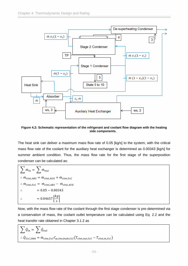
Chapter 4: Thermodynamic Design and Rating
- 53 -
Figure 4.2: Schematic representation of the refrigerant and coolant flow diagram with the heating side components.
The heat sink can deliver a maximum mass flow rate of 0.05 [kg/s] to the system, with the critical
mass flow rate of the coolant for the auxiliary heat exchanger is determined as 0.00343 [kg/s] for
summer ambient condition. Thus, the mass flow rate for the first stage of the superposition
condenser can be calculated as:
Now, with the mass flow rate of the coolant through the first stage condenser is pre-determined via
a conservation of mass, the coolant outlet temperature can be calculated using Eq. 2.2 and the
heat transfer rate obtained in Chapter 3.1.2 as
��𝑖𝑛 ��𝑜𝑢𝑡
∴ ��𝑐𝑙𝑛𝑡 𝐴𝐵𝑆 ��𝑐𝑙𝑛𝑡 𝐴𝑈𝑋 ��𝑐𝑙𝑛𝑡 𝑆 𝐶
∴ ��𝑐𝑙𝑛𝑡 𝑆 𝐶 ��𝑐𝑙𝑛𝑡 𝐴𝐵𝑆 ��𝑐𝑙𝑛𝑡 𝐴𝑈𝑋
∴
∴ [𝑘𝑔
𝑠]
��𝑖𝑛 ��𝑜𝑢𝑡
∴ ��𝑆 𝐶 𝑆𝑀𝑅 ��𝑐𝑙𝑛𝑡 𝑆 𝐶𝐶𝑝 𝑐𝑙𝑛𝑡 𝑏𝑢𝑙𝑘 𝑆 𝐶(𝑇𝑐𝑙𝑛𝑡 𝑜𝑢𝑡 𝑆 𝐶 𝑇𝑐𝑙𝑛𝑡 𝑖𝑛 𝑆 𝐶)

Chapter 4: Thermodynamic Design and Rating
- 54 -
Next, it’s possible to determine the critical mass flow rate of the coolant flowing through the
second stage of the superposition condenser by estimating the outlet temperature and using Eq.
2.2 with the heat transfer rate obtained in Chapter 3.1.2 for state 4 to TP as:
where the specific thermal capacity is an estimation of the coolant bulk temperature. The coolant
line returning to the heat sink will have a mass flow rate of 0.00460 [kg/s] at about 22.55 [°C]. This
would mean a large amount of the coolant mass flow circulating in the heating side components
has a small temperature range, that would aid the heat sink as it doesn’t have to expel large
amounts of heat energy into the atmosphere.
The process of designing the condenser unit as a superposition sizing problem ran into an
irregularity, where the total heat transfer rate from state 4 to 5 is the largest under summer ambient
conditions as mention in Chapter 3.1. Although, this cannot be said if the heat transfer rates are
looked at individually, where the heat transfer rate being higher for stage 2 under winter ambient
conditions rather than the recommended summer ambient conditions. The higher heat transfer rate
of winter conditions would yield a larger coolant critical coolant mass flow rate and subsequently a
larger heat transfer surface area for the stage 2 condenser. Therefore, as a conservative approach
to the design-sizing of the condenser unit, the sizing of stage 2 condenser will be completed under
winter ambient conditions and the thermodynamic design of the stage 1 and 2 condenser will now
be considered as separate entities forming two heat exchanger modules. The critical mass flow
rate of the coolant can be calculated as:
where the specific thermal capacity is an estimation at the coolant bulk temperature.
∴ ( )( x )(𝑇𝑐𝑙𝑛𝑡 𝑜𝑢𝑡 )
∴ 𝑇𝑐𝑙𝑛𝑡 𝑜𝑢𝑡 𝑆 𝐶
( x x )
∴ [ 𝐶]
��𝑖𝑛 ��𝑜𝑢𝑡
∴ ��𝑆 𝐶 𝑆𝑀𝑅 ��𝑐𝑙𝑛𝑡 𝑆 𝐶𝐶𝑝 𝑐𝑙𝑛𝑡 𝑏𝑢𝑙𝑘 𝑆 𝐶(𝑇𝑐𝑙𝑛𝑡 𝑜𝑢𝑡 𝑆 𝐶 𝑇𝑐𝑙𝑛𝑡 𝑖𝑛 𝑆 𝐶)
∴ (��𝑐𝑙𝑛𝑡 𝑆 𝐶)( x )( )
∴ ��𝑐𝑙𝑛𝑡 𝑆 𝐶 [𝑘𝑔 𝑠⁄ ]
��𝑖𝑛 ��𝑜𝑢𝑡
∴ ��𝑆 𝐶 𝑊𝑅𝑇 ��𝑐𝑙𝑛𝑡 𝑆 𝐶𝐶𝑝 𝑐𝑙𝑛𝑡 𝑏𝑢𝑙𝑘 𝑊𝑅𝑇(𝑇𝑐𝑙𝑛𝑡 𝑜𝑢𝑡 𝑊𝑅𝑇 𝑇𝑐𝑙𝑛𝑡 𝑖𝑛 𝑊𝑅𝑇)
∴ (��𝑐𝑙𝑛𝑡 𝑆 𝐶)( x )( )
∴ ��𝑐𝑙𝑛𝑡 𝑆 𝐶 [𝑘𝑔 𝑠⁄ ]

Chapter 4: Thermodynamic Design and Rating
- 55 -
4.3 Stage 1 Condenser (State TP to 5)
4.3.1 Preliminary Thermodynamic Design
The input parameters used to assist the preliminary thermodynamic design calculations of the
stage 1 condenser under ‘worst case’ are illustrated in Table 4.1, with the full perusal of the
preliminary design-sizing of all ambient conditions available in Appendix D 2.1.
Table 4.1: Stage 1 condenser – Thermodynamic design input parameters.
Thermodynamic Input Parameters Value/Comment
Summer ambient conditions
Thermophysical properties of state TP – 5 Section 3.1.2
Shell inner diameter: Ds 264.67 [mm]
Tube dimensions: do
di
31.8 [mm]
28.6 [mm]
Number of tubes: Nt 32 (Calculated Eq. 2.71); 24 (SW est.)
Refrigerant mass flow rate: 0.0006153 [kg/s]
Coolant mass flow rate: 0.04657 [kg/s]
Fluid Flow Input Parameters Comment
Fluid allocations: Aqua-ammonia refrigerant – shell side
Ethylene glycol water coolant – tube side
Fluid flow pattern Cross-flow (Appendix C-Figure C.15)
Coolant Thermophysical Properties Value [Units]
Tclnt,bulk 20.48 [°C]
Cp,clnt,bulk 3.7610 [kJ/kg.K]
ρclnt,bulk 1038.09 [kg/m3]
μclnt,bulk 0.0019977 [kg/m.s]
kclnt,bulk 0.499097 [W/m.K]
Prclnt,bulk 15.0930 [-]
The variable to be designed for is the tube’s heat transfer surface area, with the only unknown
dimension being the length of the tube(s).
Number of Tubes
As the number of tubes is determined using the same equation and input parameters for each of
the heat exchangers for the aqua-ammonia absorption-desorption H&R system, the calculation will
only be illustrated once with sample values for the stage 1 condenser and hereinafter the
calculated value will be given for the remaining heat exchangers. The number of tubes is
calculated by using Eq. 2.46, with the input parameters as:

Chapter 4: Thermodynamic Design and Rating
- 56 -
Single tube pass (CTP = 0.93)
Tube bundle layout set at 45° (CL = 1.00)
Ds = 264.67 [mm]
PR = 1.25 (smallest permitted pitch ratio (Thulukakanam, 2000))
do = 31.8 [mm]
where the number of tubes are rounded down to the nearest integer. The correlation of Eq. 2.46
doesn’t necessarily provide with the exact number of tubes that will fit into a fixed tube sheet, as
the formula doesn’t account for possible tube sheet stresses and equivalent diameter from shell
diameter to the closest tube. Thus, the number of tubes correlation is very conservative for a
preliminary thermodynamic design. The parameter of CL for the tube bundle layout is
approximated too low, and that the value of 1.34 rather than 1.00 gives a closer result for the
actual number of tubes that would fit into the tube sheet. This is determined by constructing the
tube sheet component using Computer Aided Design software SolidWorks, where practically only a
maximum of 24 tubes will fit into the tube sheet using the tube pitch ratio, tube bundle layout, and
tube radial dimensions.
Similar to the number of tubes calculation illustrated above, some thermodynamic design
correlations overlap between the seven heat exchanger designs. These overlapping correlations
will be illustrated with an example calculation for one heat exchanger and referenced to for the
subsequent heat exchanger designs.
Log Mean Temperature Difference
Normal convention for condensing heat exchangers would suggest the use of a mean temperature
between the in- and outlets as ΔTm = Tsat – Twall. The mean temperature difference of the stage 1
condenser can be approximated as a log mean temperature difference as the refrigerant
undergoes a phase change that doesn’t have a constant saturation temperature. The LMTD of the
stage 1 condenser is approximated as counter-flow, with the correction factor F = 1.00, due to
phase change. Therefore, with Eq. 2.4 the log mean temperature difference is calculated as
𝑁𝑡 (𝐶𝑇𝑃
𝐶𝐿)(
𝐷𝑠
𝑃𝑅 𝑑𝑜 )
∴ (
)(
x )
∴ ≅ 𝑡𝑢𝑏𝑒𝑠
𝑇𝐿𝑀𝑇𝐷𝑆 𝐶 (𝑇𝑇𝑃 𝑆𝑀𝑅 𝑇𝑐𝑙𝑛𝑡 𝑖𝑛 𝑆𝑀𝑅) (𝑇 𝑆𝑀𝑅 𝑇𝑐𝑙𝑛𝑡 𝑜𝑢𝑡 𝑆𝑀𝑅)
(𝑇𝑇𝑃 𝑆𝑀𝑅 𝑇𝑐𝑙𝑛𝑡 𝑖𝑛 𝑆𝑀𝑅
𝑇 𝑆𝑀𝑅 𝑇𝑐𝑙𝑛𝑡 𝑜𝑢𝑡 𝑆𝑀𝑅)

Chapter 4: Thermodynamic Design and Rating
- 57 -
where the temperature of the ‘Turning Point’ is approximated as 5 [°C] above the temperature of
state 5 as concluded by the investigation of Chapter 3.1.
Shell Side Heat Transfer Coefficient
State TP to 5 depicted in Fig. 3.3 represents the characteristics of a typical latent two-phase
substance. Thus the assumption is made that the shell side heat transfer coefficient for state TP to
5 can be determined by utilising the Nusselt correlation for film condensation in a tube bundle
proposed in (Kern, 1958) and the Nusselt correlation for the laminar film condensation originally
proposed in (Nusselt, 1916). The heat transfer coefficient for the stage 1 condenser is calculated
using Eq. 2.23 & 2.27, where Eq. 2.27 calculates the mean heat transfer coefficient over the tube
bundle rows. However, the number of rows of the tube bundle must be determined in order to solve
for the heat transfer coefficient. The number of rows can be calculated as the number of tubes
divided by the maximum number of tubes to fit in a horizontal line, as illustrated below:
As concluded in Chapter 3.1.1, aqua-ammonia doesn’t have a constant saturation
temperature. Therefore, it was decided to utilise a modified laminar film condensation Nusselt
correlation, which may be untested, but would yield a more conservative heat transfer coefficient.
The modification better describes the temperature boundary conditions of the latent two-phase
region of aqua-ammonia and the counter-flow ethylene glycol water.
[ ( ) (
)
( ) ]
(4.1)
This modification is made with the value of log mean temperature difference, as the log mean
temperature difference is a more descriptive representation of the mean temperatures between the
in- and outlets of the stage 1 condenser.
Alternatively, the arithmetic average temperature of (Tsat – Twall) would have resulted in an
under estimation of shell side heat transfer coefficient and the heat transfer surface area, which will
∴ ( ) ( )
(
)
∴ [ 𝐶]
𝑁𝑡 𝑚𝑎𝑥 𝐷𝑠
𝑃𝑅 x 𝑑𝑜
∴
x
∴
∴ ≅ 𝑡𝑢𝑏𝑒𝑠
𝑁𝑟𝑜𝑤𝑠 𝑁𝑡
𝑁𝑡 𝑚𝑎𝑥
∴
∴
∴ ≅ 𝑟𝑜𝑤𝑠

Chapter 4: Thermodynamic Design and Rating
- 58 -
be justified during Chapter 5 of this dissertation. Thus, the laminar film condensation heat transfer
coefficient over a single horizontal tube can be calculated as
The mean heat transfer coefficient for film condensation in a tube bundle of 5 rows can be
calculated as
Tube Side Heat Transfer Coefficient
The tube side heat transfer coefficient is determined by using the Hausen method for flow through
a circular duct, which is valid for (0.1 < Gz < 104). This is true for all of the remaining heat
exchangers to be designed, no matter the thermodynamic state or chemical composition of the
fluid (i.e. aqua-ammonia or ethylene glycol water). This is due to the low mass flow rates of both
fluids, which results in Reynolds numbers less than 2300 [-] for flow through a circular duct.
The Hausen tube side heat transfer coefficient will only be illustrated once with sample
calculations, and for the remaining heat exchangers the tube side heat transfer coefficients will be
tabulated as input parameters and output values of Re, Nu, and hi. Now, the tube side heat
transfer coefficient can be calculated as
𝑘 𝑑𝑜
[𝜌 (𝜌 𝜌𝑇𝑃) 𝑔 (𝛼𝑇𝑃
) 𝑑𝑜
𝜇 ( 𝑇𝐿𝑀𝑇𝐷 𝐶𝐹) 𝑘 ]
∴
[ ( ) ( )
( ) ]
∴ [𝑊
𝑚 𝐾]
𝑜 𝑙
𝑁 ⁄ (𝐸𝑞 )
𝑜 𝑁 ⁄
∴ ( )⁄
∴ [𝑊
𝑚 𝐾]
𝑅𝑒𝑇 ��𝑐𝑙𝑛𝑡 𝑆 𝐶
𝑁𝑡 𝜋 𝑑𝑖 𝜇𝑐𝑙𝑛𝑡 𝑏𝑢𝑙𝑘 (𝐸𝑞 𝐴 )
∴ ( )
𝜋 ( )( )
∴ [– ]
𝑃𝑒𝑏 𝑅𝑒𝑇 𝑃𝑟𝑐𝑙𝑛𝑡 𝑏𝑢𝑙𝑘
∴ [ ] (𝐶 𝑒𝑐𝑘)

Chapter 4: Thermodynamic Design and Rating
- 59 -
Overall Heat Transfer Coefficient
Assuming for the preliminary thermodynamic design of each subsequent heat exchanger including
the stage 1 condenser that fouling will be excluded from the overall heat transfer coefficient
calculation. As fouling factors require the heat transfer surface area to obtain an accurate
approximation of fouling. Therefore, by selecting Stainless Steel 304L (with k304L equal to 14.9
[W/m.K] for the specified temperature range of the stage 1 condenser) the overall heat transfer
coefficient is calculated by the following:
It’s clear that the tube side heat transfer coefficient has a far greater influence on the overall
heat transfer coefficient than that of the laminar film condensation shell side heat transfer
coefficient and the material’s thermal conductivity. Thus, the coolant creates the ‘bottleneck’ of
heat flow within the stage 1 condenser, which is a common occurrence for condensing heat
exchanger units.
𝑁𝑢𝑇 (
𝑃𝑒𝑏𝑑𝑖
𝐿)
(𝑃𝑒𝑏𝑑𝑖
𝐿) (𝐸𝑞 )
∴ ( )
( )
∴ [– ]
𝑖 𝑁𝑢𝑇 𝑘𝑐𝑙𝑛𝑡 𝑏𝑢𝑙𝑘
𝑑𝑖 (𝐸𝑞 )
∴ ( )
∴ [𝑊
𝑚 𝐾]
Assume di/L = 0.02 for preliminary thermodynamic design.
and
𝑈𝑐
𝑜
𝑖 𝑑𝑜𝑑𝑖
𝑟𝑜 (
𝑟𝑜
𝑟𝑖)
𝑘𝑚𝑎𝑡𝑒𝑟𝑖𝑎𝑙 (𝐸𝑞 )
∴
(
9
)
∴ ( 𝐸( )) ( 𝐸( )) ( 𝐸( ))
∴ 𝑈𝑆 𝐶 [𝑊
𝑚 𝐾]

Chapter 4: Thermodynamic Design and Rating
- 60 -
Heat Transfer Surface Area
Now, the thermodynamic sizing problem can be solved by determining the required length of each
tube for the stage 1 condenser, by means the following calculation:
Fouling Factors
The fouling factor for the stage 1 condenser is determined by assuming the shell side refrigerant is
a pure ammonia gas substance with Rf = 0.00017611 [m2.K/W], and the tube side coolant has a Rf
of 0.000035218 [m2.K/W]. The fouling factors and percentage over design required are calculated
with the same correlation for all the subsequent heat exchanger designs, thus, the fouling factor for
overall heat transfer coefficient will only be illustrated once for the stage 1 condenser and given
under the design-sizing selection section of the remaining six heat exchanger designs. The overall
fouling heat transfer coefficient is
where the cleanliness factor (CF) calculated as 0.9856 [-] with Eq. A.58. The total fouling
resistance (Rft) is calculated as 0.00018242 [m2.K/W] with Eq. A.57, thus the percentage over
design is calculated as
Although the oversize percentage is very small in this case, the principle will be applied to
all the remaining heat exchangers to ensure that the sizing of each heat exchanger is accurate and
practically acceptable.
𝐿 ��𝑆 𝐶
𝑈𝑆 𝐶 𝑇𝐿𝑀𝑇𝐷𝑆 𝐶(𝑁𝑡𝜋𝑑𝑜) (𝐸𝑞 )
∴
( )( 𝜋 )
∴ [𝑚]
𝑈𝑓𝐴𝑠
𝑜𝐴𝑜 𝑅𝑓 𝑜
𝐴𝑜
𝑖𝐴𝑖 𝑅𝑓 𝑖
𝐴𝑖 𝐴𝑜 (𝑑𝑜 𝑑𝑖)
𝜋𝐿𝑘𝑚𝑎𝑡𝑒𝑟𝑖𝑎𝑙 (𝐸𝑞 𝐴 )
𝑈𝑓𝐴𝑠
99 ( )
9 9 ( 99)
99
( )
𝜋( )( 9)
∴ 𝑈𝑓 [𝑊
𝑚 𝐾]
𝑂𝑆 𝑈𝑆 𝐶𝑅𝑓𝑡 (𝐸𝑞 𝐴 )
∴ ( )( )
∴ [%]

Chapter 4: Thermodynamic Design and Rating
- 61 -
4.3.2 Performance Rating of the Thermodynamic Design
Previously it was mentioned that a heat exchanger analysis consists of two problems, sizing and
rating, and now that the preliminary sizing has been completed, the rating problem or performance
rating can be solved.
NTU – Effectiveness Performance Rating
The number of heat transfer units and the effectiveness relation can be calculated using the
following:
The effectiveness is equal to 1, which is commonly expected of a condenser unit due to the phase-
change, thus satisfying the thermal heat exchanger efficiency requirement. The effectiveness is
equal to 100% for all of the ambient design conditions that is illustrated in Figure D 9.1 of Appendix
D 9.1.
Pressure Drop
The shell – and tube side pressure drop calculations are irrelevant for the stage 1 condenser, as
the layout of the heat exchanger is cross-flow orientated with TEMA shell type J. According to
(Walker, 1990) the TEMA shell type J has 1/8th the pressure drop of a regular counter flow heat
exchanger.
4.3.3 Thermodynamic Design Verification
The verification of the preliminary thermodynamic design-sizing model was completed using the
coding software EES. The verification of the heat exchanger’s heat transfer surface area can be
completed with two approaches to the formulation of sizing equations. The first method is to
duplicate the preliminary sizing as in section 4.2.2, and the second method is to use the heat
exchanger model of section 4.2.2 and determine the heat transfer rate. The first method compares
the heat exchanger’s length obtained by the two software programs, and the second method
𝑁𝑇𝑈 𝑈𝐴𝑠𝐶𝑚𝑖𝑛
𝑈𝑆 𝐶𝑁𝑡𝜋𝑑𝑜𝐿𝑡
(𝑚 𝐶𝑝 )𝑚𝑖𝑛
(𝐸𝑞 )
∴ 𝜋
∴ [– ]
휀 exp( 𝑁𝑇𝑈) (𝑇𝑎𝑏𝑙𝑒 ;𝐸𝑞 )
∴ exp( )
∴

Chapter 4: Thermodynamic Design and Rating
- 62 -
compares the heat transfer rate obtained via Eq. 2.1 to the EES heat exchanger heat transfer rate
of Eq. 2.6.
The procedure of determining if the thermodynamic design calculations are valid will only
be illustrated once for the stage 1 condenser, as the procedure is the same for all succeeding heat
exchangers in this oeuvre. As previously mentioned in Chapter 3.1.2, the thermophysical
properties of the stage 1 condenser aren’t under dispute, as the properties have already been
verified. Thus, to fully insure there are no calculation or mathematical errors in the MS Excel
coding the same thermophysical property values of the stage 1 condenser will be used for the
verification procedure for coding in EES. Full perusal of the EES coding is available in Appendix D
2.2. To keep the oeuvre concise and to the point the coded formatted equations will be illustrated
with the value obtained by EES for the said correlation.

Chapter 4: Thermodynamic Design and Rating
- 63 -
The two values of heat transfer rate are within good accordance to one another. Thus,
verifying that the MS Excel thermodynamic design model has no mathematical errors and can be
considered acceptable for the stage 1 condenser.
4.3.4 Design Sizing Selection
The shell diameter of Ds = 264.67 [mm] was selected for its length over shell diameter ratio being
within the 2 to 7 range at 2.89599 [-], as the heat exchanger will be pressurised in excess of 1
[MPa]. The tube diameter was selected based on the low number of tubes (24) the 31.8 [mm] tube
requires within the tube bundle, which saves costing in terms of less welding time spent on the
stage 1 condenser.
Commonly the tube length obtained with the design-sizing equations are rounded to an
easier to measure and manufacturable length. The heat transfer surface length of the tubes are
rounded up from 0.75586 [m] to 0.8 [m], which results in a 5.84% overdesign that accounts for
ambient conditions that exceed the summer design conditions. The coolant’s mass flow rate can
be manipulated to reduce the heat transfer rate to accommodate for the required heat of
condensation between states 5 to TP for all ambient conditions.

Chapter 4: Thermodynamic Design and Rating
- 64 -
4.4 Stage 2 Condenser (State 4 to TP)
4.4.1 Preliminary Thermodynamic Design
Stage 2 of the condenser unit has the following input parameters to assist the illustration of the
thermodynamic design calculations are set in Table 4.2, with full review of the thermodynamic
design for all ambient conditions available in Appendix D 3.1.
Table 4.2: Stage 2 condenser – Thermodynamic design input parameters.
Thermodynamic Input Parameters Value/Comment
Winter ambient conditions
Shell inner diameter: Ds 264.67 [mm]
Tube dimensions: do
di
19.1 [mm]
15.9 [mm]
Number of tubes: Nt 89 (Calculated Eq. 2.46); 68 (SW est.)
Refrigerant mass flow rate: 0.0005412 [kg/s]
Coolant mass flow rate: 0.00069 [kg/s]
Equivalent diameter: De 18.898 [mm] (Eq. A.42)
Clearance: C 4.774 [mm] (Eq. A.45)
Bundle cross-flow area: Acs 0.052936 [m2] (Eq. A.46)
Mass velocity: Gs 0.010224 [m2/s]
Number of baffles: Nb 0
Number of tube rows: Nrows 8
Tube bundle correction factor: Cn 0.98 (Table 2.3)
Fluid Flow Input Parameters Comment
Fluid allocations: Aqua-ammonia refrigerant – shell side
Ethylene glycol water coolant – tube side
Fluid flow pattern Cross-flow (Appendix C – Figure C.15)
Coolant Thermophysical Properties Value [Units]
Tclnt,bulk 25.07 [°C]
Cp,clnt,bulk 3.76985 [kJ/kg.K]
ρclnt,bulk 1036.268 [kg/m3]
μclnt,bulk 0.0017578 [kg/m.s]
kclnt,bulk 0.50166 [W/m.K]
Prclnt,bulk 13.2541 [-]
Assumption: It should be noted that the bundle cross-flow area is approximated by splitting the stage 2
condenser into two tube bundle sections with baffle spacing B = 1 [m]. The assumption is justified as the
stage 2 condenser has two inlets.

Chapter 4: Thermodynamic Design and Rating
- 65 -
The thermophysical properties of the stage 2 condenser were previously calculated in Chapter
3.1.2 for summer ambient conditions, but recent information suggested that winter ambient
conditions would yield the largest heat transfer surface area for the stage 2 condenser. Thus, the
thermophysical properties for winter ambient conditions of state 4 and TP, found in Appendix B 2 &
3, are shown in Tables 4.3 & 4.4 as:
Table 4.3: State 4 thermophysical properties for winter ambient conditions.
Thermophysical
Properties Value [Units]
T4 47.6809 [°C]
P4 515.84 [kPa]
α4 1384.1964 [kJ/kg.K]
ρ4 5.28899 [kg/m3]
μ4 1.1317E(-05) [kg/m.s]
k4 0.031027 [W/m.K]
Pr4 1.37445 [-]
Table 4.4: State TP thermophysical properties for winter ambient conditions.
Thermophysical
Properties Value [Units]
TTP 10 [°C]
PTP 515.84 [kPa]
αTP 1182.205 [kJ/kg.K]
ρTP 5.60633 [kg/m3]
μTP 2.1851E(-05) [kg/m.s]
kTP 0.060956 [W/m.K]
PrTP 1.38998 [-]
Log Mean Temperature Difference
The log mean temperature difference of the second stage condenser is calculated with the same
equation and correction factor as that of the stage 1 condenser. The correction factor of 1.00, is
caused by the specific thermal capacity of the refrigerant trending towards infinity, even though the
fluids are in a cross-flow pattern. This is evident when comparing the heat transfer rate of Eq. 2.1
to Eq. 2.2, where the heat transfer rate of Eq. 2.1 is equal to 109.3033 [W], and Eq. 2.2 is equal to
38.4222 [W]. Therefore, with this large difference in heat transfer rate it is a fair assumption that
the correction factor F = 1.00 and the log mean temperature difference calculated for counter-flow.
The log mean temperature difference is therefore calculated as:
Shell Side Heat Transfer Coefficient
Similar to stage 1 of the condenser unit, the aqueous ammonia refrigerant is allocated to flow
through the tube bundle. Although, the condenser unit has been split into two linear approximations
of the two-phase regions of aqua-ammonia, these two stages of the condenser unit aren’t best
suited to be sized with the same methodology of determining the shell side heat transfer
coefficient. As previously illustrated by Figures 3.3 & 3.5, the two-phase region of state 4 to TP has
similar behavioural characteristics to the superheated vapour region, where the temperature drops
𝑇𝐿𝑀𝑇𝐷 𝐶𝐹 [ 𝐶] (𝐸𝑞 )

Chapter 4: Thermodynamic Design and Rating
- 66 -
radically to the contrasting low decline in enthalpy. Thus, it’s assumed that the stage 2 condenser
can be treated as a ‘no-phase change’ cooling heat exchanger as the refrigerant remains highly
comprised of saturated vapour with little condensation.
The shell side heat transfer coefficient can be approximated using the Zukauskas – Nusselt
correlation of flow through a tube bundle. The Zukauskas method will result in a heat transfer
coefficient much lower than the Kern – Nusselt correlation of the stage 1 condenser. This can be
attributed to the fact that the Kern – Nusselt correlation is based on fluids condensing at a constant
temperature. Therefore, nullifying the use of the Kern – Nusselt correlation, as too little
condensation occurs within the stage 2 condenser to fully support the use of Eq. 2.23 or Eq. 4.1.
The shell side Reynolds number is calculated using Eq. A.47 as 11.6503 [-], which would suggest
the use of Eq. 2.18 for calculating the shell side heat transfer coefficient.
Tube Side Heat Transfer Coefficient
As previously illustrated, the tube side heat transfer coefficient is obtained with exactly the same
methodology as the stage 1 condenser, therefore the tube side heat transfer coefficient can be
expressed as:
Overall Heat Transfer Coefficient
The overall heat transfer coefficient of the stage 2 condenser is calculated with stainless steel 304L
as the material of the heat exchanger. The overall heat transfer coefficient is calculated as
∴ 𝑜 𝑘𝑏𝑢𝑙𝑘𝑑𝑜
( 𝑅𝑒𝐷 𝑃𝑟𝑏𝑢𝑙𝑘
(𝑃𝑟𝑏𝑢𝑙𝑘𝑃𝑟𝑤𝑎𝑙𝑙
)
)
∴
( ( ) ( ) (
)
)
∴ [𝑊
𝑚 𝐾]
𝑁𝑢𝐷 ( 𝐶𝑛 𝑅𝑒𝐷 𝑃𝑟𝑏𝑢𝑙𝑘
(𝑃𝑟𝑏𝑢𝑙𝑘
𝑃𝑟𝑤𝑎𝑙𝑙)
) (𝐸𝑞 )
𝑅𝑒𝑇 [ ] (𝐸𝑞 𝐴 )
𝑁𝑢𝑇 [ ] (𝐸𝑞 )
𝑖 [𝑊
𝑚 𝐾] (𝐸𝑞 )
𝑈𝑐
𝑜
𝑖 𝑑𝑜𝑑𝑖
𝑟𝑜 (
𝑟𝑜
𝑟𝑖)
𝑘𝑚𝑎𝑡𝑒𝑟𝑖𝑎𝑙 (𝐸𝑞 )
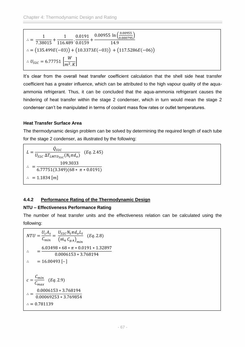
Chapter 4: Thermodynamic Design and Rating
- 67 -
It’s clear from the overall heat transfer coefficient calculation that the shell side heat transfer
coefficient has a greater influence, which can be attributed to the high vapour quality of the aqua-
ammonia refrigerant. Thus, it can be concluded that the aqua-ammonia refrigerant causes the
hindering of heat transfer within the stage 2 condenser, which in turn would mean the stage 2
condenser can’t be manipulated in terms of coolant mass flow rates or outlet temperatures.
Heat Transfer Surface Area
The thermodynamic design problem can be solved by determining the required length of each tube
for the stage 2 condenser, as illustrated by the following:
4.4.2 Performance Rating of the Thermodynamic Design
NTU – Effectiveness Performance Rating
The number of heat transfer units and the effectiveness relation can be calculated using the
following:
∴
(
9
9 )
∴ ( 𝐸( )) ( 𝐸( )) ( 𝐸( ))
∴ 𝑈𝑆 𝐶 [𝑊
𝑚 𝐾]
𝐿 ��𝑆 𝐶
𝑈𝑆 𝐶 𝑇𝐿𝑀𝑇𝐷𝑆 𝐶(𝑁𝑡𝜋𝑑𝑜) (𝐸𝑞 )
∴
( )( 𝜋 )
∴ [𝑚]
𝑁𝑇𝑈 𝑈𝑐𝐴𝑠𝐶𝑚𝑖𝑛
𝑈𝑆 𝐶𝑁𝑡𝜋𝑑𝑜𝐿𝑡
(𝑚 𝐶𝑝 )𝑚𝑖𝑛
(𝐸𝑞 )
∴ 𝜋
∴ [– ]
𝑐 𝐶𝑚𝑖𝑛
𝐶𝑚𝑎𝑥 (𝐸𝑞 )
∴
∴

Chapter 4: Thermodynamic Design and Rating
- 68 -
The effectiveness and NTU values are plotted to the standard cross-flow effectiveness vs. NTU
curve, which is illustrated in Figure D 9.2 for all ambient conditions to verify the feasibility of the
stage 2 condenser.
Though the number of transfer units stops at 5 on the standard effectiveness vs. NTU chart,
the curve can be extrapolated that the capacity ratio of 0.75 could possibly converge to an
effectiveness close to the 91% of the stage 2 condenser. If the stage 2 condenser’s coolant outlet
temperature is lower the critical mass flow rate of the coolant then the coolant mass flow rate
would inversely rise and would increase the heat transfer rate of the stage 2 condenser with very
little change to the effectiveness. The coolant outlet temperature remains at 46 [°C] and the stage 2
condenser has an estimated effectiveness of 90.497%. Therefore, meeting the thermal heat
exchanger efficiency requirements and can be classified as a feasible heat exchanger.
Note: Effectiveness is expected to be near 100% for condensers and boilers, but as the stage 2 condenser is
approximated as a cross-flow heat exchanger the effectiveness obtained might be viewed as a high
estimation. This should be kept in mind when testing the stage 2 condenser’s in- and outlet temperatures
within the entire aqua-ammonia heating & refrigeration package unit experimental setup.
Pressure Drop
The shell – and tube side pressure drop are calculated using Eq. A.50 & A.52, with the resulting
values shown in Table 4.5.
Table 4.5: Stage 2 condenser – Pressure drop.
Pressure Drop Output [Units]
Shell side pressure drop: ΔPs 0.00019 [Pa]
Tube side pressure drop: ΔPt 0.012 [Pa]
The pressure drop within the stage 2 condenser is too low to have any effect on the
thermodynamic design, therefore pressure drop is considered negligible and the stage 2
condenser won’t undergo a second iteration of design-sizing.
휀 exp 𝑁𝑇𝑈
𝑐[exp( 𝑐 𝑁𝑇𝑈 ) ] (𝑇𝑎𝑏𝑙𝑒 ;𝐸𝑞 )
∴ exp
[exp( ( ) ) ]
∴ 𝑜𝑟 [%]

Chapter 4: Thermodynamic Design and Rating
- 69 -
4.4.3 Thermodynamic Design Verification
As mentioned earlier the preliminary thermodynamic design model of MS Excel can be verified by
approximating the heat transfer rate of the sized heat exchanger model in EES. Full perusal of
EES coding for the stage 2 condenser is available in Appendix D 3.2. The output parameters of the
verification coding are illustrated in Table 4.6, with the conclusion that the comparison between the
heat transfer rate from the EES heat exchanger model and the heat transfer rate of Eq. 2.1 are
within good accordance to one another. This proves that the preliminary thermodynamic design
model is accurate. Slight differences are easily noted when comparing values such as the shell
and tube side heat transfer coefficients, where they differ with 0.2602% and 0.0355% respectively
between MS Excel and EES. These small differences are accounted to the rounding of output
values in succeeding equations in the EES verification model.
Table 4.6: Stage 2 condenser – EES verification output parameters.
Design Parameters Output [Units]
ΔTLMTD,CF 3.349 [°C]
Shell side heat transfer coefficient: ho 7.361 [W/m2.K]
Tube side heat transfer coefficient: hi 116.165 [W/m2.K]
Overall heat transfer coefficient: Uc 6.835 [W/m2.K]
Heat transfer rate: 110.516 [W]
Heat transfer rate: 109.303 [W]
Comparison percentage 1.11 [%]
Note: The stage 1 and 2 condensers have been designed for their individual ‘worst case’ scenarios, at
summer and winter ambient conditions respectively. Therefore, for the control of the aqua-ammonia heating
cycle the manipulation of coolant mass flow rate of the stage 1 condenser will be fundamental to the
effectiveness of the heating cycle at alternative ambient conditions.
4.4.4 Design Sizing Selection
If the tube diameters were to be the same for both the stage 1 and 2 condensers then the length of
the stage 2 condenser would’ve been near 3 [m], which exceeds the design selection parameter of
heat transfer surface length. Thus, for the purpose of fluid distribution in both stages of the
condenser and shorter shell length of the stage 2 condenser, a tube of do = 19.1 [mm] is selected
for the stage 2 condenser. The 19.1 [mm] tube gives a total of 68 tubes within the tube bundle,
which is within the design selection parameter. The shell housing of both the stages of the
condenser are selected with the same inner diameter nominal bore pipe, as it would be more cost
effective to purchase one pipe of diameter 264.67 [mm] than different pipe diameters for the shell
of the two condenser heat exchangers.

Chapter 4: Thermodynamic Design and Rating
- 70 -
As the design-sizing for the stage 2 condenser was completed for winter ambient
conditions, it is decided that the tube length can be rounded down from 1.230 [m] to 1.2 [m], which
is to the benefit of yearly ambient conditions being on average higher than winter ambient
conditions. Though the fouling factors would suggest an over design percentage of 4.1148%, the
stage 2 condenser has an over design percentage of 1.41%. This is a safe design assumption due
to the required length of summer ambient conditions is 47.47% lower than the modelled stage 2
condenser.
4.5 De-superheating Condenser (State 3 to 4)
4.5.1 Preliminary Thermodynamic Design
The input parameters for the preliminary design-sizing calculations of the de-superheating
condenser are set in Table 4.7.
Table 4.7: De-superheating condenser – Thermodynamic design input parameters.
Thermodynamic Input Parameters Value/Comment
Summer ambient conditions
Thermophysical properties of state 3 – 4 Section 3.1.2
Shell inner diameter: Ds 134.5 [mm]
Tube dimensions: do
di
19.1 [mm]
15.9 [mm]
Number of tubes: Nt 28 (Calculated Eq. 2.46); 15 (SW est.)
Refrigerant mass flow rate: 0.0006153 [kg/s]
Coolant mass flow rate: 0.000565 [kg/s]
Equivalent diameter: De 18.898 [mm] (Eq. A.42)
Clearance: C 4.774 [mm] (Eq. A.45)
Bundle cross-flow area: Acs 0.006725 [m2] (Eq. A.46)
Mass velocity: Gs 0.091494 [m2/s]
Baffle spacing: B 0.25 [m]
Number of tube rows: Nrows 5
Tube bundle correction factor: Cn 0.93 (Table 2.3)
Fluid Flow Input Parameters Comment
Fluid allocations: Aqua-ammonia refrigerant – shell side
Ethylene glycol water coolant – tube side
Fluid flow pattern Counter-flow (Appendix C – Figure C.13)

Chapter 4: Thermodynamic Design and Rating
- 71 -
Table 4.7 Continued:
Thermophysical Properties Value [Units]
Tclnt,bulk 69.65 [°C]
Cp,clnt,bulk 3.86643 [kJ/kg.K]
ρclnt,bulk 1015.979 [kg/m3]
μclnt,bulk 0.00072179 [kg/m.s]
kclnt,bulk 0.51983 [W/m.K]
Prclnt,bulk 5.40450 [-]
The mass flow rate of the coolant remains the same mass flow received from the stage 2
condenser, and not the de-superheating condenser’s critical mass flow rate. This is a design
decision to increase the efficiency of the cycle at the cost of possible temperature gains. In other
words the coolant’s mass flow rate isn’t reduced between the stage 2 – and de-superheating
condensers to create a single coolant line with a high temperature, rather than having two lines of
coolant with stage 2 condenser and de-superheating condenser outlet temperatures. Therefore,
the coolant outlet temperature of the de-superheating condenser can be calculated using Eq. 2.2
and the heat transfer rate obtained in Chapter 3.1.2 as
The thermodynamic design calculation output values and the corresponding correlation
used for the thermodynamic design of the de-superheating condenser are shown in Table 4.8.
Table 4.8: De-superheating condenser – Preliminary thermodynamic design output parameters.
Design Parameters Output [Units] Correlation
ΔTLMTD,CF 7.14 [°C] Eq. 2.4
Res 141.007 [-] Eq. A.47
Shell Side HTC: ho 13.1496 [W/m2.K] Eq. 2.18 & Table 2.2
ReT 4.17799 [-] Eq. A.49
NuT 3.75452 [-] Eq. 2.41
Tube Side HTC: hi 122.7502 [W/m2.K] Eq. 2.11
Overall HTC: Uc 11.6347 [W/m2.K] Eq. 2.10
Tube length: L 0.768535 [m] Eq. 2.45
��𝑖𝑛 ��𝑜𝑢𝑡
∴ ��𝐷𝐻𝐶 𝑆𝑀𝑅 ��𝑐𝑙𝑛𝑡 𝐷𝐻𝐶𝐶𝑝 𝑐𝑙𝑛𝑡 𝑏𝑢𝑙𝑘 𝐷𝐻𝐶(𝑇𝑐𝑙𝑛𝑡 𝑜𝑢𝑡 𝐷𝐻𝐶 𝑇𝑐𝑙𝑛𝑡 𝑖𝑛 𝐷𝐻𝐶)
∴ ( )( x )(𝑇𝑐𝑙𝑛𝑡 𝑜𝑢𝑡 )
∴ 𝑇𝑐𝑙𝑛𝑡 𝑜𝑢𝑡 𝑆 𝐶 [ 𝐶]

Chapter 4: Thermodynamic Design and Rating
- 72 -
From Table 4.8 it can be concluded that the aqua-ammonia refrigerant is responsible for the
hindering of heat transfer within the de-superheating condenser and that any coolant mass flow
manipulation would yield little effect on the heat capacity output of the de-superheating condenser.
4.5.2 Performance Rating of the Thermodynamic Design
The number of transfer units and the effectiveness relation is determined by using Eq. 2.8 & 2.9
and equation 1 from Table 2.1 for counter-flow heat exchangers, which is illustrated by the
following:
The effectiveness and NTU values are plotted to the standard effectiveness vs. NTU curve for
counter-flow heat exchangers, available in Appendix D 9.3.
According to Figure D 9.3 the de-superheating condenser is at the limit of performance for
a counter-flow heat exchanger, which means the assumed coolant outlet temperature of the de-
superheating condenser is at the highest allowable temperature with regards to efficiency.
Therefore, the calculated effectiveness of the de-superheating condenser in relation to the summer
ambient condition can be considered as a practically feasible heat exchanger.
𝑁𝑇𝑈 𝑈𝐴𝑠𝐶𝑚𝑖𝑛
𝑈𝐷𝐻𝐶𝑁𝑡𝜋𝑑𝑜𝐿𝑡
(𝑚 𝐶𝑝 𝑏𝑢𝑙𝑘)𝑚𝑖𝑛
∴ 𝜋
∴ [– ]
𝑐 𝐶𝑚𝑖𝑛
𝐶𝑚𝑎𝑥
𝑐 𝑚 𝐶𝑝 𝑏𝑢𝑙𝑘
��𝑐𝑙𝑛𝑡 𝑆 𝐶 𝐶𝑝 𝑐𝑙𝑛𝑡 𝑏𝑢𝑙𝑘
∴
∴
휀 exp( 𝑁𝑇𝑈( 𝑐))
𝑐 exp( 𝑁𝑇𝑈( 𝑐))
∴ exp( ( ))
exp( ( ))
∴ 𝑜𝑟 [%]

Chapter 4: Thermodynamic Design and Rating
- 73 -
Pressure Drop
The shell – and tube side pressure drop are calculated using Eqs. A.50 & A.52, with the results
recorded in Table 4.9. The pressure drops within the shell – and tube sides of the de-superheating
condenser are too small and would have little effect on the design-sizing to substantiate the
process of conducting a second design-sizing iteration.
Table 4.9: De-superheating condenser – Pressure drop.
Pressure Drop Output [Units]
Shell side pressure drop: ΔPs 0.022 [Pa]
Tube side pressure drop: ΔPt 0.011 [Pa]
4.5.3 Thermodynamic Design Verification
Full perusal of EES coding for the de-superheating condenser is available in Appendix D 4.2. The
output parameters of the verification coding are illustrated in Table 4.10. The comparison of the
heat transfer rate obtained from EES’ heat exchanger model and the heat transfer rate of Eq. 2.1
are identical. Thus, verifying the coding of MS Excel has no mathematical errors and that the
preliminary thermodynamic design is satisfactory.
Table 4.10: De-superheating condenser – EES verification output parameters.
Design Parameters Output [Units]
ΔTLMTD,CF 7.14 [°C]
Shell side heat transfer coefficient: ho 13.1497 [W/m2.K]
Tube side heat transfer coefficient: hi 122.7502 [W/m2.K]
Overall heat transfer coefficient: Uc 11.6345 [W/m2.K]
Heat transfer rate: 57.431 [W]
Heat transfer rate: 57.431 [W]
Comparison percentage -0.0015 [%]
4.5.4 Design Sizing Selection
The selection of a smaller shell diameter for the de-superheating condenser is for space saving
purposes in the z-direction, as the refrigerant flows by utilising Gibbs free energy. Thus, the
condenser units should not exceed 0.8 [m] in the z-direction within the nock of the housing
structure. The tubes are chosen to be the same tube size as the stage 2 condenser, as the smaller
19.1 [mm] tubing has a higher Reynolds number than the 31.8 [mm] tubing. The heat transfer tube
length of the de-superheating condenser is increased from 0.768535 [m] to 0.800 [m], which is a
4.094% over design that exceeds the 2.17% over design required for fouling factors.

Chapter 4: Thermodynamic Design and Rating
- 74 -
Now, to conclude the first segment of the heating components of the aqua-ammonia
heating cycle, the ethylene glycol water mixture will reach highs of 82.71 [°C] (Summer), 66.71 [°C]
(Average), and 51.08 [°C] (Winter) at the respective mass flow rates of 0.565 [g/s], 0.640 [g/s], and
0.693 [g/s].
Note: The outlet temperatures of the coolant at their respective ambient conditions are independent and
created with ideal conditions during the thermodynamic design phase. Thus, if a full flow analysis from the
heat sink to the outlet of the de-superheating condenser is to be done for all ambient conditions with the
modelled heat exchangers, the outlet temperatures achieved won’t correspond to the estimated values of the
thermodynamic design and rating without the manipulation of coolant mass flow rates. However, it must be
iterated that the concluded outlet temperatures are achievable with the modelled stage 1 & 2 and de-
superheating condensers proposed in this section, albeit it would be difficult for winter ambient conditions.
4.6 Pre-Cool Heat Exchanger (State 5 to 6 & 9 to 10)
The pre-cool heat exchanger operates between the states 5 to 6 and 9 to 10, where the pre-cool
heat exchanger adds heat from the ‘hot’ saturated liquid state 5 to the ‘cold’ saturated vapour state
9, as represented by Figure D 1.4 in Appendix D 1.4. Stated in Chapter 3.1, the pre-cool heat
exchanger is merely added to the absorption-desorption cycle to increase the refrigeration
coefficient of performance. The pre-cool heat exchanger would increase the refrigeration COP by
lowering the evaporator’s refrigerant inlet temperature, which means the evaporator would have a
larger latent area and a larger cooling capacity.
4.6.1 Preliminary Thermodynamic Design
The preliminary heat exchanger design-sizing incorporates the same shell and tube side heat
transfer coefficient correlations as used during the design-sizing of the stage 2 condenser.
Therefore, the preliminary design-sizing output values will be tabulated accordingly. The input
parameters for the preliminary design-sizing calculations of the pre-cool heat exchanger are set in
Table 4.11 as:
Mechanical material note: The subsequent heat exchangers to be designed will either have
19.1 [mm] or 31.8 [mm] stainless steel 304L tubing, and the choice of two shell diameters
264.67 [mm] or 134.5 [mm].

Chapter 4: Thermodynamic Design and Rating
- 75 -
Table 4.11: Pre-cool heat exchanger – Thermodynamic design input parameters.
Thermodynamic Input Parameters Value/Comment
Summer ambient conditions
Thermophysical properties of state 5 – 6 Appendix B 1.3
Thermophysical properties of state 9 – 10 Appendix B 1.3
Shell inner diameter: Ds 134.5 [mm]
Tube dimensions: do
di
19.1 [mm]
15.9 [mm]
Number of tubes: Nt 28 (Calculated Eq. 2.46); 15 (SW est.)
Refrigerant mass flow rate: 0.0006129 [kg/s]
Refrigerant mass flow rate: 9 0.0005986 [kg/s]
Equivalent diameter: De 18.898 [mm] (Eq. A.42)
Clearance: C 4.774 [mm] (Eq. A.45)
Bundle cross-flow area: Acs 0.006725 [m2] (Eq. A.46)
Mass velocity: Gs 0.089011 [m2/s]
Baffle spacing: B 0.25 [m]
Number of tube rows: Nrows 5
Tube bundle correction factor: Cn 0.93 (Table 2.3)
Fluid Flow Input Parameters Comment
Fluid allocations: Superheated Ammonia – shell side
Sub cooled Aqua-ammonia – tube side
Fluid flow pattern Counter-flow (Appendix C – Figure C.13)
Recorded in Table 4.12 are the thermodynamic design calculation output values and the
corresponding correlation used to determine the thermodynamic design of the pre-cool HTEX.
Table 4.12: Pre-cool heat exchanger – Preliminary design output parameters.
Design Parameters Output [Units] Correlation
ΔTLMTD,CF 14.25 [°C] Eq. 2.4
Res 183.953 [-] Eq. A.47
Shell Side HTC: ho 9.3079 [W/m2.K] Eq. 2.18 & Table 2.2
ReT 20.0219 [-] Eq. A.49
NuT 3.84190[-] Eq. 2.41
Tube Side HTC: hi 122.221 [W/m2.K] Eq. 2.11
Overall HTC: Uc 8.51922 [W/m2.K] Eq. 2.10
Tube length: L 0.39077 [m] Eq. 2.45

Chapter 4: Thermodynamic Design and Rating
- 76 -
Full review of the preliminary thermodynamic design is available in Appendix D 5.1.
4.6.2 Performance Rating of the Thermodynamic Design
The performance rating of the pre-cool heat exchanger is determined with the same methodology
as with the de-superheating condenser. Thus, to remain concise Table 4.13 depicts the NTU,
effectiveness, and pressure drops of the pre-cool heat exchanger with the resulting effectiveness
and NTU plotted to the standard counter-flow effectiveness curve in Figure D 9.4.
Table 4.13: Pre-cool heat exchanger – Performance rating.
Performance Rating Output [Units] Correlation
NTU 1.039911 [-] Eq. 2.8
Capacity Ratio: c 0.49601 [-] Eq. 2.9
Effectiveness: ε 0.5775 or 57.75 [%] Table 2.1; Eq. 1
Shell side pressure drop: ΔPs 0.020 [Pa] Eq. A.50
Tube side pressure drop: ΔPt 0.004 [Pa] Eq. A.52
The pressure drops within the shell – and tube sides are too low to substantiate the process of
conducting a second design-sizing iteration and can be considered as trivial.
The effectiveness of all the ambient design conditions fall within close proximity to one
another, and are at the expected effectiveness for a counter-flow heat exchanger. Therefore, it can
be concluded that the temperature boundary conditions are within reasonable ranges of a practical
heat exchanger application and satisfy the thermodynamic design requirements.
4.6.3 Thermodynamic Design Verification
Full review of EES coding for the pre-cool heat exchanger is available in Appendix D 5.2, where
Table 4.14 depicts the critical output parameters of the EES verification code for the pre-cool heat
exchanger.
Table 4.14: Pre-cool heat exchanger – EES verification output parameters.
Design Parameters Output [Units]
ΔTLMTD,CF 14.25 [°C]
Shell side heat transfer coefficient: ho 9.3077 [W/m2.K]
Tube side heat transfer coefficient: hi 124.563 [W/m2.K]
Overall heat transfer coefficient: Uc 8.5325 [W/m2.K]
Heat transfer rate: 42.764 [W]
Heat transfer rate: 42.698 [W]
Comparison percentage 0.1557 [%]

Chapter 4: Thermodynamic Design and Rating
- 77 -
The comparison of the heat transfer rate obtained from EES’ heat exchanger model and the heat
transfer rate of Eq. 2.1 are within 0.16% of one another. Thus, verifying the coding of MS Excel
thermodynamic design model is without any mathematical errors and the preliminary
thermodynamic design as acceptable.
4.6.4 Design Sizing Selection
The shell diameter of 134.5 [mm] and the 19.1 [mm] tubing was selected from same material
dimensions used by the de-superheating condenser. The tube length can be increased from
0.39077 [m] to 0.400 [m], which is a 2.363% over design that exceeds the 1.588% over design
required for fouling.
4.7 Venturi Nozzle and Orifice (State 6 to 7)
The concept design of the evaporator depicts three inlets, of which one is a venturi nozzle and two
orifice nozzles. The venturi nozzle needs to generate a suction force to remove excess helium
within the absorber module and re-enter the helium into the evaporator module. Commonly, the
thermodynamic design of an orifice or a venturi nozzle is considered as isothermal. The
thermodynamic design of an orifice or a venturi nozzle can be determined by using Bernoulli’s
equation for vertical fluid flow, the continuity equation for pressure drop, and a discharge equation
for the drainage mass flow rate (Engineeringtoolbox, 2015).
Bernoulli’s equation for vertical fluid flow:
(4.2)
Mass continuity equation:
[ ( )
( )]
(4.3)
where d = D2/D1.
Volumetric discharge flow rate equation:
√ (4.4)
The schematic component diagram of the venturi nozzle and orifice inlets relative to
positioning in the evaporator module and liquid column head obtained from the pyramid holding
tank is depicted by Figure 4.2.

Chapter 4: Thermodynamic Design and Rating
- 78 -
Figure 4.3: Evaporator Inlet Schematic Component Diagram
Full perusal of the venturi nozzle and orifice inlet’s control volume diagram and venturi designs are
available in Appendix D 6.1.
4.7.1 Venturi Nozzle – Thermodynamic Design
The venturi nozzle is to be designed for winter ambient conditions, as under these conditions the
refrigerant mass flow rate is at its lowest, thus, ensuring the venturi will function for the remaining
ambient design conditions. Table 4.15 shows the input parameters required to complete the
thermodynamic design of the venturi nozzle.
Common practice for smooth nozzles and venturies are that a standardised CD table found
in Table D 6.2 can approximate the discharge coefficient. The discharge coefficient for this
application is assumed to be slightly lower than convention, as the venturi’s orifice is relatively
small (selected as 2 [mm] after practical experimentation with different orifice diameters for the
venturi to work effectively) due to the very low mass flow rate and a step-down manufacturing
process instead of a smooth cross section reduction.

Chapter 4: Thermodynamic Design and Rating
- 79 -
Table 4.15: Venturi nozzle design input parameters.
Thermodynamic Input Parameters Value/Comment
Winter ambient conditions P = 515.84 [kPa]
Thermophysical properties of state 6 Appendix B 6, Table B.6
Tube dimensions: do
di = D1
19.1 [mm]
15.9 [mm]
Orifice diameter: D2 2 [mm]
Diameter ratio: d 0.125786 [-]
Refrigerant mass flow rate: 0.000539 [kg/s]
Discharge Coefficient: CD 0.9 (Assumption)
Head height difference: h1 0.6 [m]
The pressure drop at the venturi’s orifice can be calculated by rearranging Eq. 4.3, as illustrated by
the following:
To calculate the outlet velocity of the venturi nozzle,
To determine the discharge rate of the venturi nozzle,
𝑃 𝑚
𝐶𝐷𝜋
𝐷
𝜌
(𝜌 ( 𝑑 )
)
∴
𝜋
( ) ( )
( ( )
)
∴ [𝑃𝑎]
∴ 𝑃 𝑃 𝑃
∴ ( )
∴ [𝑘𝑃𝑎]
𝑃
𝜌𝑢
𝜌𝑔 𝑃
𝜌𝑢
𝜌𝑔 (𝐸𝑞 )
∴
( )
𝜋
( )
( )( )
( )𝑣
∴ 𝑢 [𝑚 𝑠⁄ ]
�� 𝐶𝐷𝐴 √ 𝑔 (𝐸𝑞 )
∴ 𝜋
( ) √ ( )( )
∴ [𝑚 𝑠⁄ ]

Chapter 4: Thermodynamic Design and Rating
- 80 -
The volumetric discharge can be converted to a more desired mass flow rate as
The venturi nozzle design can be reviewed in Appendix D 6.1, with experimental setup and results
in Appendix D 6.1 & 6.2 respectively.
4.7.2 Orifice – Thermodynamic Design Sizing
The orifice design-sizing uses the same equation set as the venturi nozzle, with the only variance
being the orifice diameter (D2 = 0.0005 m, which is the smallest drill bit that could be used for
manufacturing of the orifice nozzle) and the discharge coefficient (CD = 0.6). Therefore, the output
parameters of the orifice design are illustrated by Table 4.16 as
Table 4.16: Orifice design output parameters.
Orifice Design Output [Units]
Pressure drop: ΔP 4.03755 [kPa]
Velocity: 4.92267 [m/s]
Volume flow rate: 4.0421 x 10⁻³ [m3/s]
Mass flow rate: 0.00026195 [kg/s]
4.8 Evaporator (State 8 to 9)
The evaporator operates between the thermodynamic states 8 to 9 of Figure 3.1, which
coincidentally means it represents the refrigeration side of the aqua-ammonia absorption-
desorption cycle. Between states 8 and 9 the last mass concentration of water is removed from the
aqua-ammonia mixture to from pure ammonia, which occurs at the exact moment of evaporation.
The venturi nozzle and orifice inlets are integral to the workings of the evaporator, as the
evaporator incorporates a spray/splash evaporation method. To reiterate, the evaporator is filled
with auxiliary gas (Helium), which generates a partial pressure that works in on the aqua-ammonia
refrigerant. Thus, the refrigerant upon entering the evaporator would ‘flash’ to the thermodynamic
state 8 and in theory vaporise upon impacting the coolant filled tube bundle. Figure D 1.5 in
Appendix D 1.5 illustrates the fluid temperature variation in the evaporator. The refrigeration side of
the aqua-ammonia H&R cycle is illustrated in Figure 4.4, where the required temperatures are
shown at the respective components where heat removal is desired. The component diagram is a
theoretical representation of a heat source that adds heat to the ethylene glycol water coolant to
support boiling within the evaporator. The mean temperature difference of boiling shell and tube
heat exchangers are typically calculated as the mean temperature of the secondary fluid minus the
saturation temperature (ΔTm = Twall – Tsat), which is also known as the excess temperature. The
�� ��𝜌
∴ [𝑘𝑔 𝑠⁄ ]

Chapter 4: Thermodynamic Design and Rating
- 81 -
mean temperature difference can also be approximated as an arithmetic mean temperature
difference of ΔTam = ½(ΔT1 + ΔT2), but would result in the same value of mean temperature
difference.
Figure 4.4: Schematic representation of the refrigeration side components.
4.8.1 Preliminary Thermodynamic Design
The input parameters for the preliminary thermodynamic calculations of the evaporator are
depicted in Table 4.17. The evaporator’s thermodynamic design is approximated as three heat
exchanger models joined together, with a calculated length for the venturi inlet and two times the
calculated length for the orifice inlets. As the approach for all three sections are identical with only
variance illustrate the refrigerant inlet velocities (u2), as a result, the thermodynamic design will
only for the venturi nozzle inlet. Full review of remaining ambient conditions concerning the
respective inlets is available in Appendix D 7.1.
Table 4.17: Evaporator – Thermodynamic design input parameters.
Thermodynamic Input Parameters Value/Comment
Summer ambient conditions
Thermophysical properties of state 8 Section 3.1.3
Thermophysical properties of state 9 Appendix B 1.3
Mean temperature difference: Tm 12.75 [°C]
Shell inner diameter: Ds 264.67 [mm]
Tube dimensions: do
di
31.8 [mm]
28.6 [mm]
Number of tubes: Nt 32 (Calculated Eq. 2.46); 21 (SW est.)
Refrigerant mass flow rate: 0.0005986 [kg/s]
Coolant mass flow rate: 0.00981 [kg/s]
Inlet Quality: Qin (State 8) 0.078538
Outlet quality: Qout (State 9) 1.00

Chapter 4: Thermodynamic Design and Rating
- 82 -
Table 4.18 Continued:
Fluid Flow Input Parameters Comment
Fluid allocations: Aqua-ammonia refrigerant – shell side
Ethylene glycol water coolant – tube side
Fluid flow pattern Cross-flow (Appendix C – Figure C.22)
Inlet conditions: 3 Inlets Central venturi nozzle; 2 adjacent orifices
Coolant Thermophysical Properties Value [Units]
x 35 wt% Ethylene glycol
Tclnt,in 10 [°C]
Tclnt,out -14.5 [°C]
Tclnt,bulk / Twall -2.25 [°C]
Cp,clnt,bulk 3.52646[kJ/kg.K]
ρclnt,bulk 1063.683 [kg/m3]
μclnt,bulk 0.0060436 [kg/m.s]
kclnt,bulk 0.45463 [W/m.K]
Prclnt,bulk 46.678 [-]
Shell Side Heat Transfer Coefficient
The flow boiling heat transfer coefficient for tube bundle evaporators can be approached by
utilising (Wolvering Tube Inc, 2014) proposed tube bundle boiling prediction method as stated by
Eq. 2.31. The nucleate boiling heat transfer coefficient is predicted by using the (Cooper, 1984)
correlation given by Eq. 2.32. The convective boiling heat transfer coefficient will thus be
approximated by (Cornwell, 1989) correlation represented by Eq. 2.35 with the assumptions of:
uL = 0.01(u2)
δ = 0.05 do
Csf = 0.013 (Stainless Steel)
where uL is the refrigerant velocity flowing over the tube bundle, δ is the liquid film thickness, and
Csf is the experimental constant that is dependent on surface-fluid combination. The refrigerant
velocity flowing over the tube bundle is assumed to be 0.01 of the velocity from the venturi nozzle,
due to the stream ejected by the venturi will first hit a flat distribution disc before splashing onto the
tube bundle.
The nucleate boiling and peak heat flux values are calculated as
��𝑛𝑢𝑐𝑙𝑒𝑎𝑡𝑒 𝜇 𝑓𝑔 [𝑔(𝜌 𝜌9)
𝜎]
[𝐶𝑝 (𝑇𝑤𝑎𝑙𝑙 𝑇𝑠𝑎𝑡)
𝐶𝑠𝑓 𝑓𝑔𝑃𝑟 𝑛 ]
(𝐸𝑞 )

Chapter 4: Thermodynamic Design and Rating
- 83 -
The value of peak heat flux for pure ammonia was obtained from EES’ critical heat flux function as
822.635 [kW/m2], which is in great proximity of the value obtained by Eq. 2.34 for aqua-ammonia to
pure ammonia ebullition. Thus, validating the peak heat flux value and illustrating that the
evaporator lies beneath the critical point in the nucleate boiling regime on the boiling curve, which
ensures that ‘burnout’ doesn’t occur.
To calculate the nucleate boiling heat transfer coefficient correlation of Cooper (1984),
To calculate the liquid film Reynolds number,
To determine the convective boiling heat transfer coefficient,
∴ ( )( ) [ ( )
( )]
[ ( ( ))
( )( )]
∴ [𝑊
𝑚 ]
∴ ( )( )[ ( )( )( )]
∴ [𝑊
𝑚 ]
and
��𝑚𝑎𝑥 𝐶𝑐𝑟 𝑓𝑔[𝜎𝑔𝜌9 (𝜌 𝜌9)]
(𝐸𝑞 ), with Ccr = 0.12
𝑛𝑏 (𝑃𝑟 (𝑅𝑝)) ( (𝑃𝑟))
𝑀𝑁𝐻
��𝑛𝑢𝑐𝑙𝑒𝑎𝑡𝑒 (𝐸𝑞 )
∴ ( ( ))( ( )) ( )( )
∴ [𝑊
𝑚 𝐾]
𝑅𝑒𝛿 𝜌 𝑢𝑙𝛿
𝜇 (𝐸𝑞 )
∴ ( )( )( )
∴ [– ]
𝑐𝑏 (𝑅𝑒𝛿 )(𝑃𝑟𝑙
) (𝑘𝑙𝛿) (𝐸𝑞 )
∴ ( )( ) (
)
∴ [𝑊
𝑚 𝐾]

Chapter 4: Thermodynamic Design and Rating
- 84 -
The bundle boiling heat transfer coefficient becomes,
Tube Side Heat Transfer Coefficient
The tube side heat transfer coefficient utilises the (Hausen, 1959) Nusselt correlation given in Eq.
2.41, which is the same method used during the previous heat exchanger’s thermodynamic design.
Thus, the output values of the tube side are represented by Table 4.18 as
Table 4.18: Evaporator – Tube side heat transfer coefficient.
Design Parameters Output [Units] Correlation
ReT 3.444 [-] Eq. A.49
NuT 3.963 [-] Eq. 2.41
Tube Side HTC: hi 62.9892 [W/m2.K] Eq. 2.11
Now that the tube side heat transfer coefficient is known, it can be concluded that the lower heat
transfer coefficient of the coolant will be open to manipulation. The coolant mass flow rate and inlet
temperature can be altered when necessary, to keep the refrigeration cycle operating at optimum
conditions. In other words, to ensure that the evaporation process takes place within the two-phase
region with minimal over evaporation into the superheated region.
Overall Heat Transfer Coefficient and Heat Transfer Surface Area
The calculation of the overall heat transfer coefficient and the length of the tubes aren’t concise
and have been illustrated, thus the entire evaporator thermodynamic design output results are
summarised by Table 4.19. The tube side heat transfer coefficient is considerably lower than its
shell side opposite, thus suggesting that the coolant controls the outcome of Uc values.
Table 4.19: Evaporator – Thermodynamic design output parameters.
Design Parameters Output [Units]
Shell side heat transfer coefficient: ho 179.853 [kW/m2.K]
Tube side heat transfer coefficient: hi 62.9892 [W/m2.K]
Overall heat transfer coefficient: Uc 56.2769 [W/m2.K]
Tube length: LVenturi 0.5635 [m]
Tube length: LOrifice 0.5635 [m]
Tube length: LEvap 1.6905 [m]
𝑏𝑢𝑛𝑑𝑙𝑒 ( 𝑛𝑏 𝑐𝑏
)
(𝐸𝑞 )
∴ ( )
∴ [𝑊
𝑚 𝐾]

Chapter 4: Thermodynamic Design and Rating
- 85 -
4.8.2 Performance Rating of the Thermodynamic Design
Table 4.20, with the NTU, effectiveness, capacity ratio, records the performance rating of the
evaporator as:
Table 4.20: Evaporator – Performance rating.
Performance Rating Output [Units] Correlation
NTU 32.155 [-] Eq. 2.8
Capacity Ratio: c 0.05976 [-] Eq. 2.9
Effectiveness: ε 1.00 or 100 [%] Table 2.1; Eq. 4
The effectiveness vs. NTU curve of the evaporator’s design performance is available in Appendix
D 9.5 for all ambient conditions. The effectiveness vs. NTU curve of Figure D 9.5 illustrates that the
evaporator has a 100% effectiveness, which is common for boiling heat exchangers. The pressure
drops within the shell and tube sides are too small to have any significant effect on the design-
sizing and have been excluded from the thermodynamic design calculations of the evaporator
module.
4.8.3 Thermodynamic Design Verification
Perusal of EES coding for the evaporator’s thermodynamic design verification is available in
Appendix D 7.2, with Table 4.21 depicting the critical output parameters thereof. The conclusion
that can be drawn from the comparison is that there are no mathematical errors in the
determination of the evaporator’s thermodynamic design, as the heat transfer rate comparison is
within 0.2%. Therefore, the calculation of the thermodynamic design for the evaporator can be
considered as acceptable.
Table 4.21: Evaporator – EES verification output parameters.
Design Parameters Output [Units]
ΔTm 12.75 [°C]
Shell side heat transfer coefficient: ho 179.799 [kW/m2.K]
Tube side heat transfer coefficient: hi 63.1166 [W/m2.K]
Overall heat transfer coefficient: Uc 56.385 [W/m2.K]
Heat transfer rate: 849.95 [W]
Heat transfer rate: 848.31 [W]
Comparison percentage 0.1939 [%]

Chapter 4: Thermodynamic Design and Rating
- 86 -
4.8.4 Design Sizing Selection
The 264.67 [mm] shell diameter was selected for the evaporator as it has a length to diameter ratio
that falls within the specified range of 2 to 7. The 31.8 [mm] tubing was selected as it uses
approximately 50 less tubes than what the 19.1 [mm] tubing would’ve used. Although, the larger
tube has a slightly lower tube side Reynolds number the manufacturing costs are cut on the
assembling and welding times. A fouling factor over design percentage of 13.57% is added to the
tube length, thus, resulting in a heat transfer tube length of 1.920 [m].
4.9 Auxiliary-Regenerative Heat Exchanger (Weak and Strong Aqua-Ammonia Solutions)
The auxiliary and regenerative heat exchangers operate between the absorber (absorption) and
bubble pump (desorption) components as illustrated in Figure 3.3. The regenerative heat
exchanger plays an important role in support of the bubble pump module and the auxiliary heat
exchanger increases the absorbability of weak solution aqua-ammonia in the absorber module.
The temperature changes versus unit surface area of the regenerative and auxiliary heat
exchangers are represented in Figures D 1.6 & 1.7 of Appendix D, respectively.
The thermodynamic design of both the auxiliary and regenerative heat exchangers use the
(Zukauskas, 1987) shell side heat transfer coefficient correlation and (Hausen, 1959) tube side
heat transfer coefficient correlation. Which are the same correlations used for the stage 2
condenser, de-superheating condenser, and pre-cool heat exchanger.
4.9.1 Regenerative Heat Exchanger – Preliminary Thermodynamic Design
Represented by Table 4.22 are the input parameters required for ‘worst case’ preliminary design-
sizing calculations of the regenerative heat exchanger, with the full review of the remaining
ambient condition’s preliminary thermodynamic design available in Appendix D 8.1.
Table 4.22: Regenerative heat exchanger – Thermodynamic design input parameters.
Thermodynamic Input Parameters Value/Comment
Winter ambient conditions
Thermophysical properties of state (ws: 1 & 2) Section 3.1.4
Thermophysical properties of state (ss: 1 & 2) Section 3.1.4
Correction factor: F 0.89 (Figure A.3(b))
Log mean temperature difference: ΔTLMTD 10.6284 [°C]
Shell inner diameter: Ds 0.34768 [mm]
Tube dimensions: do
di
31.8 [mm]
28.6 [mm]
Number of tubes: Nt 49 (Calculated Eq. 2.46); 44 (SW est.)

Chapter 4: Thermodynamic Design and Rating
- 87 -
Table 4.22 continued:
Number of tube rows: Nrows 7 (SW est.)
Tube bundle correction factor: Cn 0.96 (Table 2.3)
Equivalent diameter: De 31.464 [mm] (Eq. A.42)
Clearance: C 7.95 [mm] (Eq. A.45)
Bundle cross-flow area: Acs 0.069536 [m2] (Eq. A.46)
Mass velocity: Gs 0.064677 [m2/s]
Heat transfer rate: 293.2575 [W] (Eq. 2.1)
Refrigerant mass flow rate: 0.003971 [kg/s]
Secondary refrigerant mass flow rate: 0.004497 [kg/s]
Inlet Quality: Qss,1 -0.001
Outlet quality: Qss,2 0.0084
Fluid Flow Input Parameters Comment
Fluid allocations: Strong solution aqua-ammonia – shell side
Weak solution aqua-ammonia – tube side
Fluid flow pattern Cross-flow (Appendix C – Figure C.26)
The preliminary thermodynamic design output values are tabulated in Table 4.23, with the
corresponding correlations used for each parameter. In comparison, the shell side heat transfer
coefficient is the lower value of the two sided of heat transfer coefficient, which indicates to the
shell side heat transfer coefficient being the impeding factor on the outcome of overall heat transfer
coefficient. The short tube length is due to a low heat capacity requirement and large shell
diameter.
Table 4.23: Regenerative heat exchanger – Preliminary design output parameters.
Design Parameters Output [Units] Correlation
ΔTLMTD,XF 10.63 [°C] Eq. 2.4
Res 2.937 [-] Eq. A.47
Shell Side HTC: ho 45.4930 [W/m2.K] Eq. 2.18 & Table 2.2
ReT 7.570 [-] Eq. A.49
NuT 4.18143 [-] Eq. 2.41
Tube Side HTC: hi 69.4907 [W/m2.K] Eq. 2.11
Overall HTC: Uc 26.1364 [W/m2.K] Eq. 2.10
Tube length: L 0.2402 [m] Eq. 2.45

Chapter 4: Thermodynamic Design and Rating
- 88 -
4.9.2 Regenerative Heat Exchanger – Performance Rating of the Thermodynamic Design
The number of transfer units and the effectiveness of the regenerative heat exchanger are
demonstrated by Table 4.24 as:
Table 4.24: Regenerative heat exchanger – Performance rating.
Performance Rating Output [Units] Correlation
NTU 1.61730 [-] Eq. 2.8
Capacity Ratio: c 0.88102 [-] Eq. 2.9
Effectiveness: ε 0.5981 or 59.81% Table 2.1; Eq. 3
The effectiveness, NTU, and capacity ratio values above are plotted to the standard effectiveness
vs. NTU curve in Appendix D 9.6 for all ambient conditions, which can be used to verify the
feasibility and temperature boundary conditions of the regenerative heat exchanger. As illustrated
by Figure D 9.6, the intersection of the effectiveness and NTU output values fall just beneath the
capacity ratio curve, which indicates that the regenerative heat exchanger’s in- and outlet
temperatures are satisfactory. The effectiveness vs. NTU output parameters strongly advise that
the regenerative heat exchanger is feasible and transfers heat to the strong solution with a thermal
efficiency of 59.81%.
4.9.3 Regenerative Heat Exchanger – Thermodynamic Design Verification
The EES coding for the regenerative heat exchanger is available in Appendix D 8.2. The critical
output parameters of the EES verification code are recorded in Table 4.25.
Table 4.25: Regenerative heat exchanger – EES verification output parameters.
Design Parameters Output [Units]
ΔTLMTD,XF 10.63 [°C]
Shell side heat transfer coefficient: ho 45.221 [W/m2.K]
Tube side heat transfer coefficient: hi 68.166 [W/m2.K]
Overall heat transfer coefficient: Uc 25.948 [W/m2.K]
Heat transfer rate: 291.18 [W]
Heat transfer rate: 293.26 [W]
Comparison percentage -0.7074 [%]
The comparison of the heat transfer rate obtained from EES’ heat exchanger model and the heat
transfer rate of Eq. 2.1 vary by less than 0.71%, which would indicate to minute differences in the
output values used to obtain the heat transfer rate of the EES heat exchanger model. Input
parameters such as dinner/L play a miniscule role in the outcome of the heat transfer rate, but it

Chapter 4: Thermodynamic Design and Rating
- 89 -
might be the reason for the slight difference in the comparison percentage. Therefore, it is
concluded that the EES verification model is within acceptable range to the preliminary
thermodynamic design model and a secondary thermodynamic design iteration isn’t required.
4.9.4 Regenerative Heat Exchanger – Design Selection
The preliminary thermodynamic design was completed for the ‘worst case’ scenario of winter
ambient conditions, but the regenerative heat exchanger has great influence on the functionality of
the aqua-ammonia H&R cycle. The remaining ambient conditions require a smaller heat transfer
surface area and with the modelled heat exchanger the heat transfer rate can’t be manipulated as
the previously mentioned heat exchangers would’ve been. This is due to the working fluids of the
regenerative heat exchanger being fixed by the bubble pump generator. Therefore, the
regenerative heat exchanger is classified into three heat exchangers that cater for the three
ambient conditions. The heat transfer tube lengths with factored over design percentages are
recorded in Table 4.26 as:
Table 4.26: Regenerative heat exchanger – Tube lengths.
Ambient Design Condition Length [m] Over Design [%]
Summer 0.055 19.794 (19.537% Foul)
Average 0.160 18.624 (16.62% Foul)
Winter 0.280 16.588 (13.696% Foul)
The shell diameter selection will be clarified during the design-sizing selection of the auxiliary heat
exchanger as the two heat exchanger entities will be merged to form one heat exchanger module.
4.9.5 Auxiliary Heat Exchanger – Preliminary Thermodynamic Design
The final heat exchanger has its input parameters shown in Table 4.27, which are required to
complete the preliminary design calculations of the auxiliary heat exchanger.
Table 4.27: Auxiliary heat exchanger – Thermodynamic design input parameters.
Thermodynamic Input Parameters Value/Comment
Winter ambient conditions
Thermophysical properties of state (ws: 2 & 3) Section 3.1.4
Shell inner diameter: Ds 0.34768 [mm]
Tube dimensions: do
di
31.8 [mm]
28.6 [mm]
Number of tubes: Nt 49 (Calculated Eq. 2.46); 44 (SW est.)
Heat transfer rate: 608.834 [W] (Eq. 2.1)

Chapter 4: Thermodynamic Design and Rating
- 90 -
Table 4.27 continued:
Refrigerant mass flow rate: 0.003971 [kg/s]
Secondary refrigerant mass flow rate: 0.003803 [kg/s]
Equivalent diameter: De 31.464 [mm] (Eq. A.42)
Clearance: C 7.95 [mm] (Eq. A.45)
Bundle cross-flow area: Acs 0.017384 [m2] (Eq. A.46)
Mass velocity: Gs 0.21877 [m2/s]
Baffle spacing: B 0.25 [m]
Number of tube rows: Nrows 7
Tube bundle correction factor: Cn 0.96 (Table 2.3)
Fluid Flow Input Parameters Comment
Fluid allocations: Ethylene glycol water coolant – shell side
Weak solution aqua-ammonia – tube side
Fluid flow pattern Counter-flow (Appendix C – Figure C.28)
The thermodynamic design of the auxiliary heat exchanger resulted in the output values tabulated
in Table 4.28 along with the corresponding correlations used for each parameter. The preliminary
thermodynamic design of summer ambient condition is considerably less than the winter ambient
design, as illustrated by the MS Excel design model in Appendix D 8.1.
Table 4.28: Auxiliary heat exchanger – Preliminary thermodynamic design output parameters.
Design Parameters Output [Units] Correlation
ΔTLMTD,CF 3.06 [°C] Eq. 2.4
Res 3.57039 [-] Eq. A.47
Shell Side HTC: ho 70.0399 [W/m2.K] Eq. 2.18 & Table 2.2
ReT 3.54601 [-] Eq. A.49
NuT 3.79207 [-] Eq. 2.41
Tube Side HTC: hi 61.6875 [W/m2.K] Eq. 2.11
Overall HTC: Uc 30.8511 [W/m2.K] Eq. 2.10
Tube length: L 1.4672 [m] Eq. 2.45
The shell and tube side heat transfer coefficients are fairly close to one another, with the
tube side heat transfer coefficient being slightly lower than shell side. Thus, the weak aqua-
ammonia solution is forming the ‘bottleneck’ on the path of heat transfer.

Chapter 4: Thermodynamic Design and Rating
- 91 -
4.9.6 Auxiliary Heat Exchanger – Performance Rating of the Thermodynamic Design
The number of transfer units and the effectiveness of the auxiliary heat exchanger are
demonstrated by Table 4.29, with the resulting output parameters plotted to the standard
effectiveness vs. NTU curve in Appendix D 9.7 to verify the practical feasibility of coolant outlet
temperature for the auxiliary heat exchanger.
Table 4.29: Auxiliary heat exchanger – Performance rating.
Performance Rating Output [Units] Correlation
NTU 11.8119 [-] Eq. 2.8
Capacity Ratio: c 0.84953 [-] Eq. 2.9
Effectiveness: ε 0.86717 or 86.717% Table 2.1; Eq. 1
Fig. D 9.7 demonstrated that the intersection of the effectiveness and NTU values on the standard
counter-flow curve is slightly below the expected efficiency of a typical counter-flow heat
exchanger. This indicates that the outlet temperature of the coolant could be increased, but would
mean an increase in the heat transfer surface area and in the cost of the auxiliary heat exchanger.
If the coolant outlet temperature is to be raised by 1 [°C] the length required of a single tube would
increase by 473.38 [mm] for 44 tubes, which accumulate to an extra 20.830 [m] of tubing. Thus,
the auxiliary heat exchanger’s thermodynamic design will remain as calculated.
4.9.7 Auxiliary Heat Exchanger – Thermodynamic Design Verification
The verification design-sizing coding, with formatted equations and solutions for the auxiliary heat
exchanger is available in Appendix D 8.3, however the critical output parameters of the EES
verification code are shown in Table 4.30.
Table 4.30: Regenerative heat exchanger – EES verification output parameters.
Design Parameters Output [Units]
ΔTLMTD,CF 3.06 [°C]
Shell side heat transfer coefficient: ho 70.172 [W/m2.K]
Tube side heat transfer coefficient: hi 61.966 [W/m2.K]
Overall heat transfer coefficient: Uc 30.953 [W/m2.K]
Heat transfer rate: 610.84 [W]
Heat transfer rate: 608.83 [W]
Comparison percentage 0.3299 [%]

Chapter 4: Thermodynamic Design and Rating
- 92 -
4.9.8 Auxiliary heat exchanger – Design Sizing Selection
The shell diameter selected for the auxiliary and regenerative heat exchanger is larger than the
shell diameters proposed for the stage 1 and 2 condensers, and the evaporator module. The
reason for the larger shell selection is the L/Ds ratio, which is approximated at 4.22 [-] instead of
8.094 [-] for the 264.67 [mm] shell. The heat transfer tube length of the auxiliary heat exchanger
can now be determined as L = 1.7 [m], which falls within the design selection parameter. The
auxiliary heat exchanger has a 15.865% over design that exceed the 15.731% required by fouling.
4.10 Conclusion
To conclude the thermodynamic design and rating, a summative sizing and rating table is compiled
for the seven heat exchangers for an aqua-ammonia heating and refrigeration package unit in
Table 4.31. The thermodynamic design of each heat exchanger resulted in satisfying the design
selection requirements for heat transfer tube length, number of tubes, and length over shell
diameter for pressurised vessels. The performance rating of the heat exchangers revealed that
each heat exchangers were within the expected efficiencies of standard counter/cross-flow heat
exchangers, which pointing towards the conclusion that the inlet and outlet temperature conditions
of the heat exchangers are satisfactory. Therefore, the heating side heat exchangers will
approximately produce a heating capacity of 1.62 [kW] for summer ambient conditions and 1.37
[kW] for winter ambient conditions. The heating side heat exchangers will hence produce a heating
capacity COP of 1.5 and 1.4, respectively, and consequently satisfy the requirement for a heating
capacity COP > 1.3. The evaporator or cooling side heat exchanger will approximately produce a
cooling capacity of 0.85 [kW] for summer ambient conditions and 0.77 [kW] for winter ambient
conditions, with cooling capacity COP of 0.76 and 0.77, respectively. Hence, the requirement of the
cooling capacity COP is also satisfied.
Table 4.31: Summative thermodynamic design table of the heat exchangers for an aqua-ammonia absorption-desorption heating and refrigeration cycle.
HTEX Flow Pattern Ds [mm] do/di [mm] Nt L [m] ε [%] Capacity [W]
S1C Cross-flow 264.67 31.8 / 28.6 24 0.800 100 726.5
S2C Cross-flow 264.67 19.1 / 15.9 68 1.200 90.497 72.9
DHC Counter-flow 134.5 19.1 / 15.9 15 0.800 90.091 57.4
PC Counter-flow 134.5 19.1 / 15.9 15 0.400 57.75 42.7
EVAP Cross-flow 264.67 31.8 / 28.6 21 1.920 100 848.3
REGEN Cross-flow 347.68 31.8 / 28.6 44 0.280 59.81 293.3
AUX Counter-flow 347.68 31.8 / 28.6 44 1.700 86.741 608.8

Chapter 4: Thermodynamic Design and Rating
- 93 -
Each of the abovementioned heat exchangers were verified to be within good accordance
of the heat transfer rate obtained by Eq. 2.1 and the EES heat exchanger model with Eq. 2.6, but
further validation is required to prove that accurate correlation selection was utilised in the
calculation of each heat exchanger’s thermodynamic design model. The following chapter will
focus on the validation of the thermodynamic design process, as the sized heat exchanger models
will be utilised during the mechanical design of Appendix E. Validation is essential for any design
process as it ensures the correct methods were utilised during the design calculation stages.

- 94 -
Chapter 5
5 THERMODYNAMIC DESIGN VALIDATION
Introduction
Chapter 5 of the oeuvre focuses on the validation of the previously sized heat exchangers of
Chapter 4. Typical engineering convention dictates that the thermodynamic design of heat
exchangers are validated experimentally or by comparing the calculated design models to
previously published design models. However, heat exchangers with aqua-ammonia as its
refrigerant don’t have an undisputed design model to which this study could compare its results.
Due to project limitation stressed in Chapter 1, the validation of the thermodynamic design process
will be completed mathematically and by utilising standard heat exchanger references. The
validation process will see the predicted overall heat transfer coefficient compared to typically
expected overall heat transfer coefficient ranges of heat exchangers with similar fluid
configurations.

Chapter 5: Thermodynamic Design Validation
- 95 -
5.1 Thermodynamic Design Validation Process
The correlations used to determine the surface area As and the mean temperature difference (ΔTm
or ΔTLMTD) are considered to be truthful, as these correlations are universally applied with their
respective governing parameters. The calculated overall heat transfer coefficient Uc of Eq. 2.6
requires a degree of validation to prove that accurate correlations were utilised in determining the
shell and tube side heat transfer coefficients. Ideally, the overall heat transfer coefficient is
validated by comparing the predicted Uc values to the experimentally obtained values of Uc.
Although, it’s possible to validate the predicted overall heat transfer coefficient values by
comparing the designed heat exchangers Uc with typically expected ranges of overall heat transfer
coefficients. Table 5.1 illustrates the typically expected Uc values of different heat exchanger
configurations that are applicable to the heat exchangers of this oeuvre. The overall heat transfer
coefficients of condensers and evaporators are commonly ‘controlled’ or ‘bottle necked’ by the
secondary refrigerant, thus emphasizing the fundamental role that the coolant has to contribute to
the Uc value.
Table 5.1: Typical ranges of overall heat transfer coefficients for shell and tube heat exchangers.
Typical Shell and Tube Heat Exchanger Overall Heat Transfer Coefficients
Application
Working Fluid Allocation Typical OHTC [W/m2.K]
Source(s) Tube Side Shell Side Minimum Maximum
S1C
Water Ammonia 300 1200 [2]
Water Aqueous Vapour 1000 1500 [1], [4], [5]
S2C & DHC
Water Gases 20 300 [4]
Water Gases 17 280 [2], [3], [5]
Brine Gases 15 250 [4]
Brine Gases 17 280 [2], [3], [5]
EVAP
Steam Pool: Aqueous
Solution
500 1000 [1]
Water Refrigerant 425 850 [2], [3]
AUX
Water Water 800 1500 [1], [2], [3], [4], [5]
Water Brine 600 1200 [1], [2], [3], [4]
Liquid Liquid 150 1200 [2]
REGEN
Water Water 800 1500 [1], [2], [3], [4], [5]
Aqueous Solution Aqueous Solution 1400 2800 [5]
Liquid Liquid 150 1200 [2]

Chapter 5: Thermodynamic Design Validation
- 96 -
The sources of Tables 5.1 & 5.2 are numbered as follows:
1. (Blackmonk Engineering, 2009)
2. (Engineers Edge, 2016)
3. (H&C Heat Transfer Solutions, 2014)
4. (Engineering Page, 2016)
5. (Edwards, 2008)
It is very important to note that these overall heat transfer coefficient ranges are estimated for heat
exchangers with higher heat capacities and mass flow rates than that of the heat exchangers of
Chapter 4. These ranges are commonly used as indicators to the order of magnitude of Uc values,
whereby actual calculation of the overall heat transfer coefficient might result in values lower or
higher than the listed values.
In some instances, further validation is possible by comparing the calculated heat transfer
coefficients with the typical heat transfer coefficients of Table 5.2. These ranges are guidelines for
both the shell and tube side heat transfer coefficients.
Table 5.2: Typical ranges of heat transfer coefficients for shell and tube heat exchangers.
Typical Film Heat Transfer Coefficients
Application Working Fluid
Typical HTC [W/m2.K]
Source(s) Minimum Maximum
S1C Condensing Ammonia 2840 5680 [2], [3]
S2C & DHC Gases 15 250 [2], [3]
PC Gases 15 250 [2], [3]
EVAP Evaporating Ammonia 1135 2270 [2], [3]
AUX Water 1700 11350 [2], [3]
REGEN Water 1700 11350 [2], [3]
5.2 Stage 1 Condenser
The overall heat transfer coefficient of the sized stage 1 condenser model of Chapter 4.3.1 is
clearly below the typically expected overall heat transfer coefficient ranges for ammonia outside –
water inside of Table 5.1. It was previously concluded in Chapter 4.3.1 that the overall heat transfer
coefficient of the stage 1 condenser is haltered by the tube side heat transfer coefficient. The tube
side heat transfer coefficient halters the Uc value with its laminar flow regime and low Reynolds
number, which is attributed to the low coolant mass flow rates.
Validation of the overall heat transfer coefficient can be achieved by isolating the Uc term of
Eq. 2.31, with the assumption that all thermophysical properties and ΔTLMTD remains constant. The
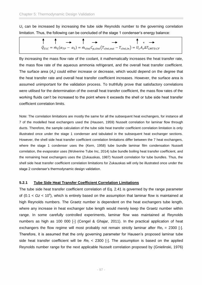
Chapter 5: Thermodynamic Design Validation
- 97 -
Uc can be increased by increasing the tube side Reynolds number to the governing correlation
limitation. Thus, the following can be concluded of the stage 1 condenser’s energy balance:
By increasing the mass flow rate of the coolant, it mathematically increases the heat transfer rate,
the mass flow rate of the aqueous ammonia refrigerant, and the overall heat transfer coefficient.
The surface area (As) could either increase or decrease, which would depend on the degree that
the heat transfer rate and overall heat transfer coefficient increases. However, the surface area is
assumed unimportant for the validation process. To truthfully prove that satisfactory correlations
were utilised for the determination of the overall heat transfer coefficient, the mass flow rates of the
working fluids can’t be increased to the point where it exceeds the shell or tube side heat transfer
coefficient correlation limits.
Note: The correlation limitations are mostly the same for all the subsequent heat exchangers, for instance all
7 of the modelled heat exchangers used the (Hausen, 1959) Nusselt correlation for laminar flow through
ducts. Therefore, the sample calculation of the tube side heat transfer coefficient correlation limitation is only
illustrated once under the stage 1 condenser and tabulated in the subsequent heat exchanger sections.
However, the shell side heat transfer coefficient correlation limitations differ between the 7 heat exchangers,
where the stage 1 condenser uses the (Kern, 1958) tube bundle laminar film condensation Nusselt
correlation, the evaporator uses (Wolverine Tube Inc, 2014) tube bundle boiling heat transfer coefficient, and
the remaining heat exchangers uses the (Zukauskas, 1987) Nusselt correlation for tube bundles. Thus, the
shell side heat transfer coefficient correlation limitations for Zukauskas will only be illustrated once under the
stage 2 condenser’s thermodynamic design validation.
5.2.1 Tube Side Heat Transfer Coefficient Correlation Limitations
The tube side heat transfer coefficient correlation of Eq. 2.41 is governed by the range parameter
of (0.1 < Gz < 104), which is entirely based on the assumption that laminar flow is maintained at
high Reynolds numbers. The Graetz number is dependent on the heat exchangers tube length,
where any increase in heat exchanger tube length would merely keep the Graetz number within
range. In some carefully controlled experiments, laminar flow was maintained at Reynolds
numbers as high as 100 000 [-] (Cengel & Ghajar, 2011). In the practical application of heat
exchangers the flow regime will most probably not remain strictly laminar after Ret = 2300 [-].
Therefore, it is assumed that the only governing parameter for Hausen’s proposed laminar tube
side heat transfer coefficient will be Ret < 2300 [-]. The assumption is based on the applied
Reynolds number range for the next applicable Nusselt correlation proposed by (Gnielinski, 1976)
��𝑆 𝐶 �� (𝛼𝑇𝑃 𝛼 ) ��𝑐𝑙𝑛𝑡𝐶𝑝 𝑐𝑙𝑛𝑡(𝑇𝑐𝑙𝑛𝑡 𝑜𝑢𝑡 𝑇𝑐𝑙𝑛𝑡 𝑖𝑛) 𝑈𝑐𝐴𝑠 𝑇𝐿𝑀𝑇𝐷 𝐶𝐹

Chapter 5: Thermodynamic Design Validation
- 98 -
for transitional flow through a circular duct. Thus, the maximum coolant mass flow rate is
calculated by re-arranging Eq. A.49 as:
5.2.2 Shell Side Heat Transfer Coefficient Correlation Limitations
The tube bundle laminar film condensation heat transfer coefficient output value isn’t directly
influenced by the increase in refrigerant mass flow rate. However, if the mass flow rate were to be
increased to the point where the vapour velocity is larger than 10 [m/s], then vapour shear will
occur and demand a definite correlation change from the tube bundle laminar film condensation
heat transfer coefficient in Eq. 2.27 proposed by Kern (1958) to the Butterworth (1977) inundation
and vapour shear heat transfer coefficient of Eq. 2.28. The vapour velocity is determined at the
minimum flow area between the tubes and can be approximated as 5 times the mean inlet velocity.
Therefore, by determining the inlet cross-sectional area and factoring it into a simple conservation
of mass equation with the mean vapour velocity limit of 2 [m/s], it would result in a maximum inlet
mass flow rate of:
5.2.3 Overall Heat Transfer Coefficient Validation Results
The progression of the overall heat transfer coefficient values versus steady incremental increases
in tube side Reynolds numbers are plotted and illustrated in Figure 5.1. The tube side Reynolds
number is chosen as it represents the controlling factor on Uc value increases. The tube side
Reynolds numbers are increased from 40 to 2300 in increments of 0.01 [kg/s], where the initial
mass flow rate starts at 0.04 [kg/s] and ends at the maximum of 2.47694 [kg/s]. As illustrated by
the legend at the bottom of Figure 5.1, the purple curve with circle symbols represent the Uc values
of aqua-ammonia to ethylene glycol water heat transfer. The light blue curve with square symbols
represents the overall heat transfer coefficient values of aqua-ammonia to water heat transfer, and
the dark blue curve represent ammonia to water heat transfer.
��𝑐𝑙𝑛𝑡 𝑚𝑎𝑥 𝑅𝑒𝑡 𝑁𝑡 𝜋 𝑑𝑖 𝜇𝐵
∴ ( 𝜋)( )( )
∴ [𝑘𝑔
𝑠]
�� 𝑚𝑎𝑥 𝜌𝑇𝑃𝐴𝑖𝑛𝑙𝑒𝑡𝑢𝑚
∴ ( )(𝜋
( ) ( 𝑥 )) ( )
∴ [𝑘𝑔
𝑠]

Chapter 5: Thermodynamic Design Validation
- 99 -
The working fluids of the stage 1 condenser are replaced with pure ammonia and water to
better represent Uc values that compare with the typical overall heat transfer coefficient ranges of
Table 5.1. The substituted aqua-ammonia with pure ammonia is of comparable thermophysical
properties in terms of pressure (939.54 kPa) and saturation temperature (23 °C). Ethylene glycol
water is replaced with water of equivalent thermophysical properties in relation to the bulk fluid
temperature. The bulk fluid temperature of water is determined with the original heat transfer rate
of the stage 1 condenser and an estimated specific heat capacity.
Points 1 and 3 mark the initial and limit of aqua-ammonia to ethylene glycol water’s overall
heat transfer coefficient values. Points 2 and 4 represent the initial and limit values of both the
aqua-ammonia-to-water and ammonia-to-water overall heat transfer coefficients. The two curves
are identical in shape as they lie on top of each other. This would suggest that the overall heat
transfer coefficient does not differentiate between pure ammonia and 99 wt% aqua-ammonia, as
water has control over the outcome of the Uc simulation.
Figure 5.1: Stage 1 Condenser - Overall heat transfer coefficient vs. tube side Reynolds number simulation model output plot.
0 100 300 500 700 900 1100 1300 1500 1700 1900 2100 230075
100
125
150
175
200
225
250
275
300
325
Tube Side Reynolds Number [-]
Uc
[W/m
2K
]
Uc (Lower Boundary) = 300 [W/m2K]
1
2
3
4

Chapter 5: Thermodynamic Design Validation
- 100 -
The results of the Uc simulation curves are illustrated in Tables 5.3 and 5.4, where Table
5.3 represents the initial conditions of the stage 1 condenser and Table 5.4 shows the limiting
boundary conditions. The initial input parameters of the aqua-ammonia-to-water and ammonia-to-
water condenser simulations are calculated at the original heat transfer rate of the stage 1
condenser, as calculated in Chapter 3.1.2. The limiting boundary condition occurs where the shell
or tube side heat transfer coefficients meet their respective correlation limits.
The results of Table 5.3, supports the claim that the overall heat transfer coefficient does
not discriminate between the 99 wt% aqua-ammonia and 100% pure ammonia to water heat
transfer. This is evident with the 0.2% difference in initial Uc values.
Table 5.3: Stage 1 condenser - The initial boundary conditions for 3 permutations of working fluids.
Initial boundary conditions: Aq - B Aq - W Am - W
Coolant mass flow rate: 0.046569 [kg/s] 0.041871 [kg/s] 0.041871 [kg/s]
Tube side: Ret 43.24 [-] 77.78 [-] 77.78 [-]
Tube side HTC: hi 91.17 [W/m2.K] 103.91 [W/m2.K] 103.91 [W/m2.K]
Refrigerant mass flow rate: 0.0006153 [kg/s] 0.0006153 [kg/s] 0.0006185 [kg/s]
Shell side HTC: ho 6694.43 [W/m2.K] 6694.43 [W/m2.K] 8156.89 [W/m2.K]
Heat transfer rate: 726.503 [W] 726.503 [W] 726.552 [W]
Overall heat transfer coefficient: Uc 80.27 [W/m2.K] 91.214 [W/m2.K] 91.438 [W/m2.K]
Further investigation was conducted with lower mass concentrations of ammonia in water mixtures,
of which the results are shown in Table 5.5.
It’s evident from Table 5.4 that at higher Reynolds numbers the ethylene glycol water
mixture creates a higher Uc value than the equivalent water coolant fluid. The Reynolds numbers of
both ethylene glycol water and water are at 2300 [-], but their respective Prandtl numbers differ
considerably with water having a much lower Prandtl number. This is the main contributing factor
that ethylene glycol water has a higher heat transfer coefficient.
The three working fluid permutations of Uc are lower than the typically expected overall heat
transfer coefficient for condensing ammonia-to-water. This can be attributed to the tube side heat
transfer coefficient reaching its correlation limit Ret = 2300 [-], before the shell side could reach its
mass flow rate and mean vapour velocity limits. Therefore, the optimal operating conditions of the
modelled stage 1 condenser, with aqua-ammonia and ethylene-glycol water, results in a maximum
Uc of 249.090 [W/m2K]. If the tube side heat transfer coefficient correlation were to be changed to
(Gnielinski, 1976) Nusselt correlation for transitional flow through circular ducts, the overall heat
transfer coefficients would easily enter the typical Uc ranges of Table 5.1.

Chapter 5: Thermodynamic Design Validation
- 101 -
Table 5.4: Stage 1 condenser - The limit boundary conditions for 3 permutations of working fluids.
Limit boundary conditions: Aq - B Aq - W Am - W
Coolant mass flow rate: 2.47694 [kg/s] 1.235 [kg/s] 1.235 [kg/s]
Tube side: Ret 2300 [-] 2300 [-] 2300 [-]
Tube side HTC: hi 296.30 [W/m2.K] 268.45 [W/m2.K] 268.45 [W/m2.K]
Refrigerant mass flow rate: 0.032720 [kg/s] 0.018149 [kg/s] 0.017091 [kg/s]
Shell side HTC: ho 6694.43 [W/m2.K] 6694.43 [W/m2.K] 8156.89 [W/m2.K]
Heat transfer rate: (Eq. 2.26) 38.6335 [kW] 21.4291 [kW] 20.0785 [kW]
Overall heat transfer coefficient: Uc 249.090 [W/m2.K] 227.044 [W/m2.K] 228.433 [W/m2.K]
The curves of Figure 5.2 illustrate the temperature versus enthalpy of aqueous ammonia at
different ammonia mass concentrations and their respective ‘turning points’. As previously claimed
in Chapter 3.1.1, to the right of the ‘turning point’ is where the temperature decreases more rapidly
than enthalpy, and to the left of the ‘turning point’ the temperature vs. enthalpy exhibits the
characteristics of a typical latent two-phase substance. Thus, the assumption of 2 stages of the
condenser was created.
Figure 5.2: Temperature vs. enthalpy of different mass concentrations of ammonia in water mixtures.

Chapter 5: Thermodynamic Design Validation
- 102 -
Closer investigation was conducted at 90 wt% ammonia in water, where the ‘turning point’ was
found to be at the quality of Q = 0.63. Figure 5.3 illustrates the linear enthalpy estimation of both
the 90 and 99 wt% ammonia in water. The red line represents the linear enthalpy estimation of the
90 wt% aqua-ammonia, and the blue line represents the 99 wt% ammonia in water. The dot-dash
lines illustrate construction lines similar to that of the ‘turning point’ investigation of Chapter 3.1.1.
Figure 5.3: Enthalpy vs. quality investigation of ‘turning point’ for 0.9 and 0.99 mass concentrations ammonia in water.
0 0.2 0.4 0.6 0.8 10
200
400
600
800
1000
1200
1400
1600
1800
Quality [-]
En
thalp
hy [
kJ/k
g]
TP
TP
Linear Enthalpy Est (x = 0.9)
Linear Enthalpy Est (x = 0.99)
0.7 0.8 0.9 1
800
1000
1200
1400
1600
Quality [-]
En
thalp
hy [
kJ/k
g]
TP
TP
Q = 0.63 Q = 0.94
Enthalpyest

Chapter 5: Thermodynamic Design Validation
- 103 -
The temperature boundary conditions of the coolant for the 90 wt% simulation are
calculated to equate the log mean temperature difference of the 99 wt% stage 1 condenser.
Entering the thermophysical properties of state TP0.9 and the same refrigerant mass flow rate as
the 99 wt% stage 1 condenser into the stage 1 condenser thermodynamic design model yielded
the results tabulated in Table 5.5.
Table 5.5: The comparison table of the stage 1 condenser simulation model with 90 & 99 wt% aqua-ammonia and water as coolant.
S1C: Mass concentration comparison x = 0.9 x = 0.99
ΔTLMTD,CF 5.098 [°C] 5.099 [°C]
Coolant mass flow rate: 0.01211 [kg/s] 0.041871 [kg/s]
Tube side: Ret 11.25 [-] 77.78 [-]
Tube side HTC: hi 74.905 [W/m2.K] 103.91 [W/m2.K]
Refrigerant mass flow rate: 0.0006153 [kg/s] 0.0006153 [kg/s]
Shell side HTC: ho 6152.92 [W/m2.K] 6694.43 [W/m2.K]
Heat transfer rate: (Eq. 2.27) 455.594 [W] 726.503 [W]
Heat transfer rate: (Eq. 2.27) 961.78 [W] 799.36 [W]
Overall heat transfer coefficient: Uc 66.139 [W/m2.K] 91.214 [W/m2.K]
It can be concluded from Table 5.5 that the 0.9 mass concentration has a lower overall heat
transfer coefficient, which is due to the lower tube side heat transfer coefficient. The low tube side
heat transfer coefficient can be attributed to the lower coolant mass flow rate, which is directly
connected to the refrigerant mass flow rate. The mass flow rate of the aqua-ammonia remains
constant for both mass concentrations due to the assumption that the bubble pump generator will
boil-off aqua-ammonia at the same rate for both mass concentrations.
The differing overall heat transfer coefficient results from Tables 5.4 and 5.5 clearly support
the claim that the stage 1 condenser can’t be sized by assuming pure ammonia thermophysical
properties, when there is a mass concentration lower than 98 wt% aqua-ammonia. The differences
in heat transfer rates of Table 5.4 also indicates to the reality that the stage 1 condenser can’t be
sized by assuming pure ammonia thermophysical properties, even if the mass concentration is
0.99. As the heat transfer surface area could result in an over estimation of the required heat
transfer surface area. The differences in heat transfer rates of Table 5.5 and the behavioural
characteristics of two-phase aqua-ammonia can support the assumption that an aqua-ammonia
condenser can be split into two stages of the condenser unit (latent condensing heat exchanger
and vapour cooling heat exchanger). In section 5.3 the assumption that the second stage of the
condenser unit may be approached as a gas-to-brine heat exchanger will be proved to be
acceptable.

Chapter 5: Thermodynamic Design Validation
- 104 -
5.2.4 Shell Side Heat Transfer Coefficient Validation Results
As previously mentioned, the tube bundle laminar film condensation HTC isn’t influenced by mass
flow rates and Reynolds numbers, but it is greatly influences by the wall temperature of the tubes.
The ethylene glycol water solution’s inlet and outlet temperatures effect the wall temperature.
Assuming the coolant outlet temperature remains the same as the initial stage 1 condenser model
and the inlet temperature is decreased in small increments, the shell side heat transfer coefficient
would theoretically decrease. Figure 5.4 and the results in Table 5.6 support the assumption that
the laminar film condensation heat transfer coefficient proposed by (Nusselt, 1916) can be
approached as a log mean temperature difference, as proposed by Eq. 4.1.
Figure 5.4: Stage 1 condenser – Shell side heat transfer coefficient vs. temperature difference simulation model output plot.
The dark blue curve with circle symbols represent the results of Eq. 4.1 (log mean temperature
difference method), the light blue square symbol curve represents the results obtained by Eq. 2.23
(mean temperature difference method). These two curves are identically shaped and occupy the
4 5 6 7 8 9 10 11 12 13 14 15 16 17 18 19 20 21 22 23 24 25 264200
4400
4600
4800
5000
5200
5400
5600
5800
6000
6200
6400
6600
6800
Temperature Difference[C]
ho
[W/m
2K
]
ho (Lower Boundary) = 5680 [W/m2K]
1
2
3
4

Chapter 5: Thermodynamic Design Validation
- 105 -
same coordinates, though the two methods yield different results for the same input parameters.
The third curve, with triangular symbols, represents the results obtained with pure ammonia
substance and the mean temperature difference method.
The three points of comparison of Fig. 5.4 are set at a coolant inlet temperature of 5 [°C].
The heat transfer coefficient output value of the (aqua-ammonia) log mean temperature difference
method (at point 2) is slightly less conservative by 2.788%, than the result of the (aqua-ammonia)
mean temperature difference method (at point 3). Although, the log mean temperature difference
method is slightly less conservative than the mean temperature difference method, the counter-
flow log mean temperature better represents the two-phase mean temperature difference between
aqua-ammonia solutions (with temperature glide) and the secondary refrigerant. Point 4 of Figure
5.4 illustrates the equivalent to points 2 & 3 with pure ammonia as refrigerant, which has a shell
side heat transfer coefficient approximately 6.02% higher than that of point 2 and 8.98% higher
than that of point 3.
Table 5.6: Stage 1 condenser – Shell side heat transfer coefficient output values.
Points Tclnt,in ΔTLMTD or MTD ho Uc
1 18.404 [°C] 5.01 [°C] (LMTD) 6699.73 [W/m2.K] 80.27 [W/m2.K]
2 5 [°C] 10.503 [°C] (LMTD) 5563.48 [W/m2.K] 65.442 [W/m2.K]
3 5 [°C] 11.72 [°C] (MTD) 5412.56 [W/m2.K] 65.420 [W/m2.K]
4 5 [°C] 9.224 [°C] (MTD) 5898.36 [W/m2.K] 65.442 [W/m2.K]
As shown in Table 5.6 the overall heat transfer coefficient of points 2 and 3 are near
identical, which would only leave the mean temperature difference to influence the heat transfer
surface area. If it were assumed that for points 2 and 3 the heat transfer rates are identical, then
the heat transfer surface area of point 2 would be 11.59% larger than that of point 3. Thus
supporting the decision to use Eq. 4.1 and the counter-flow log mean temperature difference as a
conservative and elegant approach to determine the thermodynamic design for first segment of the
latent two-phase region of aqua-ammonia solutions.
5.2.5 Thermodynamic Design Validation Conclusion
The conclusions that can be made from the results obtained in section 5.2 are:
The assumption that the condenser unit can’t be sized by assuming pure ammonia
thermophysical properties is valid.
The mean temperature difference of the laminar film condensation heat transfer coefficient
is better represented with a counter-flow log mean temperature difference when dealing
with temperature-glide in aqua-ammonia solutions, despite the fact it is 2.788% less
conservative.

Chapter 5: Thermodynamic Design Validation
- 106 -
The mean temperature difference of the heat transfer rate in Eq. 2.3 is better represented
with the counter-flow log mean temperature difference when dealing with temperature
gliding mixtures, as it is 11.59% more conservative. Therefore, the mean temperature
difference method would underestimate the total heat transfer surface area required for the
thermodynamic design of the latent like region of aqueous ammonia solutions.
The overall heat transfer coefficient of a condensing heat exchanger is greatly influenced
by the secondary refrigerant (coolant).
The overall heat transfer coefficient output values were below the typical Uc range values,
which are to be expected of a condensing heat exchanger with low refrigerant and coolant
mass flow rates with laminar flow regimes.
Therefore, it can be concluded that accurate correlations were utilised in calculating the stage 1
condenser’s thermodynamic design. The design-sizing parameters of the stage 1 condenser are
now utilised in the mechanical design consideration phase, with which the manufacturing and
assembly drawings are created. The mechanical design considerations of the stage 1 condenser
are available in Appendix E 1, and the manufacturing and assembly drawings are available in
Appendix E 2.
5.3 Stage 2 Condenser
The heat transfer coefficient results from the modelled stage 2 condenser in Chapter 4.4.1 indicate
that the shell side heat transfer coefficient impedes heat from being transferred. Thus, for the
validation of the stage 2 condenser the mass flow rate of the refrigerant will be increased, whilst
maintaining constant thermophysical properties for both aqua-ammonia and ethylene-glycol water.
The energy balance of the stage 2 condenser is
The Uc simulation will start at the Res of the original sized stage 2 condenser model of Chapter
4.4.1 and will continue increasing until one of the correlation limits are reached.
The heat transfer coefficient correlation limitations of the second stage of the condenser
unit are determined similarly to the limitations of the stage 1 condenser, therefore the tube side
heat transfer coefficient correlation limitations are tabulated into Table 5.7.
Table 5.7: Stage 2 condenser – Tube side heat transfer coefficient correlation limitations.
Correlation Limit Parameters Limit
Tube side: Ret 2300
Maximum coolant mass flow rate: 2.1048 [kg/s]
��𝑆 𝐶 �� (𝛼 𝛼𝑇𝑃) ��𝑐𝑙𝑛𝑡𝐶𝑝 𝑐𝑙𝑛𝑡(𝑇𝑐𝑙𝑛𝑡 𝑜𝑢𝑡 𝑇𝑐𝑙𝑛𝑡 𝑖𝑛) 𝑈𝑐𝐴𝑠 𝑇𝐿𝑀𝑇𝐷 𝐶𝐹

Chapter 5: Thermodynamic Design Validation
- 107 -
The shell side staggered tube bundle Nusselt correlation proposed in (Zukauskas, 1987) is largely
influenced by the Reynolds number for flow across the tube bundle. The incremental increase of
refrigerant mass flow rate will increase the Res and consequently the heat transfer coefficient. The
correlation of Eq. 2.18 has its limitation recorded in Table 5.8 as:
Table 5.8: Stage 2 condenser – Shell side heat transfer coefficient correlation limitations.
Correlation Limit Parameters Limit
Shell side: Res 500
Maximum coolant mass flow rate: 0.02323 [kg/s]
5.3.1 Overall Heat Transfer Coefficient Validation Results
Figure 5.5 represents the growth of the overall heat transfer coefficient values versus steady
incremental increases of shell side Reynolds numbers. The shell side Reynolds number was
chosen for the x-axis as it signifies the governing factor of the Uc correlation output value
increases. The shell side Reynolds numbers are increased from an initial 11.7 to the limit of 500 [-],
with 0.01 [kg/s] increments. The initial position, represented by point 1 on Figure 5.5, is the original
stage 2 condenser model as illustrated in Chapter 4.4.1.
Figure 5.5: Stage 2 condenser – Overall heat transfer coefficient vs. shell side Reynolds number simulation model output plot.
0 100 200 300 400 5005
10
15
20
25
30
Shell Side Reynolds Number [-]
Uc
[W/m
2K
]
Uc (Lower Boundary) = 15 [W/m2K]
Initial Uc = 6.78 [W/m2K]
Limit Uc = 25.16 [W/m2K]
1
2
3

Chapter 5: Thermodynamic Design Validation
- 108 -
The initial overall heat transfer coefficient is fairly lower than the lower boundary of typical
Uc ranges, which can be attributed to the very low mass flow rates achieved by an absorption-
desorption cycle. The overall heat transfer coefficient simulation reaches the shell side heat
transfer coefficient correlation limit at 25.16 [W/m2.K], which falls inside the expected Uc ranges of
gases-to-brine heat transfer. Presented in Table 5.9 are the output values of points 1, 2, and 3.
Table 5.9: Stage 2 Condenser – Overall heat transfer coefficient vs. shell side Reynolds numbers simulation model output values.
Stage 2: Uc Simulation 1 2 3
Coolant mass flow rate: 0.0006925 [kg/s] 0.006219 [kg/s] 0.029726 [kg/s]
Tube side: Ret 0.464 [-] 4.166 [-] 19.915 [-]
Tube side HTC: hi 116.165 [W/m2.K] 119.237 [W/m2.K] 127.508 [W/m2.K]
Refrigerant mass flow rate: 0.0005412 [kg/s] 0.004860 [kg/s] 0.02323 [kg/s]
Shell side: Res 11.7 [-] 104.6 [-] 500 [-]
Shell side HTC: ho 7.3610 [W/m2.K] 17.711 [W/m2.K] 33.114 [W/m2.K]
Heat transfer rate: 109.303 [W] 981.548 [W] 4691.64 [W]
Overall heat transfer coefficient: Uc 6.78 [W/m2.K] 15 [W/m2.K] 25.165 [W/m2.K]
The shell side heat transfer coefficient does have a sharp increase in response to the gains in
Reynolds numbers. This is due to two factors: Reynolds numbers increase more rapidly with a gas
state fluid than a liquid state fluid; and transitional flow occurs at lower Reynolds numbers for shell
side than that of tube side. The Uc simulation model limit of point 3 doesn’t exceed the tube side
heat transfer coefficient correlation limit of Ret = 2300. If the shell side heat transfer coefficient
were substituted with Eqs. 2.19 or 2.20 the overall heat transfer coefficient could in theory increase
even further. This however isn’t recommended, as a steady increase in refrigerant mass flow rate
would only result in larger heat transfer rate requirements and impractically large heat exchangers.
Therefore, if the heat capacity of the stage 2 condenser is to be increased, it should be increased
well into the turbulent flow regime.
Recorded in Table 5.10 is the heat exchanger comparison made between 0.9 and 0.99
mass concentration aqua-ammonia. The comparison is made at the initial conditions of the stage 2
condenser simulation model, that way the comparison is equivalent to the sized stage 2 condenser
model of Chapter 4.4. Included is the assumption that the mass flow rate of aqua-ammonia
remains constant for both stage 2 condenser’s mass concentrations simulations. The temperature
boundary conditions of the coolant for the 90 wt% simulation are calculated to equate the log mean
temperature difference of the 99 wt% stage 2 condenser.
The overall heat transfer coefficient of the 90 wt% aqua-ammonia is near four times greater
than the 99 wt% aqua-ammonia, which can be attributed to the slightly higher liquid quality of bulk

Chapter 5: Thermodynamic Design Validation
- 109 -
fluid thermophysical properties of the 90 wt% aqua-ammonia. The overall heat transfer coefficient
of the 90 wt% aqua-ammonia does however fall within the typical range of gas-to-brine heat
exchangers.
The required heat transfer rate to cool the 90 wt% stage 2 condenser is more than four
times greater than the 99 wt% stage 2 condenser. The heat transfer surface area of the 90 wt%
stage 2 condenser would be 31.12% larger than its counterpart.
Table 5.10: The comparison table of the sized stage 2 condenser model with 90 & 99 wt% aqua-ammonia and ethylene glycol water as coolant.
S2C: Mass concentration comparison x = 0.9 x = 0.99
ΔTLMTD,CF 3.434 [°C] 3.348 [°C]
Coolant mass flow rate: 0.0015227 [kg/s] 0.0006925 [kg/s]
Tube side: Ret 1.664 [-] 0.464 [-]
Tube side HTC: hi 119.050 [W/m2.K] 116.165 [W/m2.K]
Refrigerant mass flow rate: 0.0005412 [kg/s] 0.0005412 [kg/s]
Shell side: Res 2.098 [-] 11.7 [-]
Shell side HTC: ho 30.125 [W/m2.K] 7.3610 [W/m2.K]
Heat transfer rate: (Eq. 2.27) 487.017 [W] 109.30 [W]
Overall heat transfer coefficient: Uc 23.040 [W/m2.K] 6.780 [W/m2.K]
5.3.2 Thermodynamic Design Validation Conclusion
In conclusion, the overall heat transfer coefficient validation of section 5.3.1 yielded coherent
results that proved that adequate correlations were utilised in the thermodynamic design of the
second stage of the condenser unit. The knowledge obtained from the mass concentration
comparison results supported the assumption that the condenser unit using an aqua-ammonia
refrigerant can be split into two thermodynamic heat exchanger designs and that the second stage
of the condenser unit be treated as a gas-to-brine heat exchanger. Furthermore, it can be
concluded that the stage 1 condenser will decrease in surface area with decreasing wt% of
ammonia in water and the stage 2 condenser would increase in heat transfer surface area with
decreasing wt% of ammonia in water.
The performance rating proves that the sized stage 2 condenser model can be implemented
as a practical application with an expected thermal efficiency around 90%. Consequently, the
sizing model of Chapter 4.4 may be utilised to further the mechanical design considerations and
manufacturing drawings of Appendix E 3.

Chapter 5: Thermodynamic Design Validation
- 110 -
5.4 De-superheating Condenser
The modelled de-superheating condenser of Chapter 4.5 indicated that the shell side heat transfer
coefficient impedes the heat from being transferred, and thus is considered as the controlling factor
of the overall heat transfer coefficient. The Uc simulation will see the increase of shell side
Reynolds numbers from the originally modelled Res = 141.007 [-] (as presented in Table 4.9) to the
Res limit in 0.01 [kg/s] increments. Thus, the de-superheating condenser’s energy balance is:
As the de-superheating condenser uses the exact same correlations to determine its shell
and tube side heat transfer coefficients as the stage 2 condenser; the correlation limitations will be
the same. Therefore, recorded in Tables 5.11 and 5.12 are the tube side correlation limitations and
the shell side correlation limitations, respectively.
Table 5.11: De-superheating condenser – Tube side heat transfer coefficient correlation limitations.
Correlation Limit Parameters Limit
Tube side: Ret 2300 [-]
Maximum coolant mass flow rate: 0.31097 [kg/s]
Table 5.12: De-superheating condenser – Shell side heat transfer coefficient correlation limitations.
Correlation Limit Parameters Limit
Shell side: Res 500 [-]
Maximum refrigerant mass flow rate: 0.002182 [kg/s]
5.4.1 Overall Heat Transfer Coefficient Validation Results
Presented in Figure 5.6 is the overall heat transfer coefficient simulation of the de-superheating
condenser. The overall heat transfer coefficient reaches the shell side Reynolds number limit at
18.064 [W/m2.K], which falls within the typical Uc range of a gas-to-brine heat exchanger. Table
5.13 illustrates the input and output values of the points one, two, and three in Fig. 5.6. The tube
side Reynolds number remain noticeably low throughout the Uc simulation, which is to be expected
from the small increases in refrigerant mass flow rates. As the coolant and refrigerant mass flow
rates are co-dependent. The shell side Reynolds numbers increase rapidly with the small
increases in mass flow rate, due to its superheated vapour state. Therefore, the overall heat
transfer coefficient simulation model doesn’t exceed the tube side heat transfer coefficient
correlation limit of Ret = 2300 [-].
Thus, to further the Uc value of the de-superheating condenser the shell side heat transfer
coefficient correlation needs to be changed to Eq. 2.19 for Reynolds numbers between 500 and
��𝐷𝐻𝐶 �� (𝛼 𝛼 ) ��𝑐𝑙𝑛𝑡𝐶𝑝 𝑐𝑙𝑛𝑡(𝑇𝑐𝑙𝑛𝑡 𝑜𝑢𝑡 𝑇𝑐𝑙𝑛𝑡 𝑖𝑛) 𝑈𝑐𝐴𝑠 𝑇𝐿𝑀𝑇𝐷 𝐶𝐹

Chapter 5: Thermodynamic Design Validation
- 111 -
1000 [-]. Although, it should be noted that further increases in refrigerant mass flow rate in the
laminar regime will only cause the heat transfer surface area to increase to impractical sizes.
Therefore, if the mass flow rate and heat capacity of the refrigerant is to be increased, it should be
increased to Reynolds numbers in the turbulent regime. The output values of turbulent heat
transfer coefficients are typically much higher than that of laminar heat transfer coefficients.
Figure 5.6: De-superheating condenser – Overall heat transfer coefficient vs. shell side Reynolds number simulation model output plot.
Table 5.13: De-superheating condenser – Overall heat transfer coefficient vs. shell side Reynolds numbers simulation model output values.
De-superheating: Uc Simulation 1 2 3
Coolant mass flow rate: 0.0005649 [kg/s] 0.0011650 [kg/s] 0.0020032 [kg/s]
Tube side: Ret 4.178 [-] 8.617 [-] 14.82 [-]
Tube side HTC: hi 122.75 [W/m2.K] 125.012 [W/m2.K] 127.681 [W/m2.K]
Refrigerant mass flow rate: 0.0006153 [kg/s] 0.001269 [kg/s] 0.002182kg/s]
Shell side: Res 141.007 [-] 290.82 [-] 500 [-]
Shell side HTC: ho 13.150 [W/m2.K] 17.566 [W/m2.K] 21.818 [W/m2.K]
Heat transfer rate: 57.431 [W] 118.447 [W] 203.667 [W]
Overall heat transfer coefficient: Uc 11.635 [W/m2.K] 15 [W/m2.K] 18.064 [W/m2.K]
100 200 300 400 500 600 70010
12
14
16
18
20
22
24
Shell Side Reynolds Number [-]
Uc
[W/m
2K
] Limit Uc = 18.064 [W/m2K]
Initial Uc = 11.63 [W/m2K]1
2
3
Uc (Lower Boundary) = 15 [W/m2K]

Chapter 5: Thermodynamic Design Validation
- 112 -
5.4.2 Thermodynamic Design Validation Conclusion
In conclusion, the Uc simulation model proves that the thermodynamic design process of the de-
superheating condenser to be acceptable. The calculated performance rating supports the claim
that the thermodynamic design of the de-superheating condenser is practically feasible, with
realistically expected coolant outlet temperatures. Therefore, the sizing model concluded in
Chapter 4.5.4 may be utilised to further the mechanical design considerations of the de-
superheating condenser in Appendix E 1, and help create the manufacturing and assembly
drawings of Appendix E 4.
5.5 Pre-Cool Heat Exchanger
The fluid configuration of the pre-cool heat exchanger doesn’t have a corresponding typical overall
heat transfer coefficient range in Table 5.1, but its shell and tube side heat transfer coefficients can
be validated individually. As the pre-cool heat exchanger uses exactly the same equations for the
shell and tube heat transfer coefficient correlations as the de-superheating condenser, the
correlations limitations will be similar. The sized heat exchanger model of Chapter 4.6 suggests
that the shell side heat transfer coefficient impedes heat transfer from occurring and is therefore
considered as the controlling factor. Presented in Table 5.14 is the shell side heat transfer
coefficient correlation limitation to be used in the validation simulation model. The tube side heat
transfer coefficient correlation is assumed as proven to be acceptable, due to the previous work of
sections 5.2, 5.3 and 5.4.
Table 5.14: Pre-cool heat exchanger – Shell side heat transfer coefficient correlation limitations.
Correlation Limit Parameters Limit
Shell side: Res 500 [-]
Maximum refrigerant mass flow rate: 9 0.0016273 [kg/s]
The validation process of the pre-cool heat exchanger doesn’t require an energy balance or
constant tube side thermophysical properties, although it does require the incremental increase of
shell side Reynolds numbers and constant ammonia thermophysical properties. Shell side
Reynolds numbers increase from an initial value of 183.943 [-] to the correlation limit of 500 [-] in
0.01 [kg/s] increments. The lower boundary of the typical range of heat transfer coefficient for
gases is 15 [W/m2.K] (Engineers Edge, 2016).
5.5.1 Shell Side Heat Transfer Coefficient Validation Results
Demonstrated in Figure 5.7 is the shell side heat transfer coefficient simulation versus shell side
Reynolds numbers, where the simulated increase in heat transfer coefficient reaches its correlation
limit before entering the typical expected range of gas heat transfer.

Chapter 5: Thermodynamic Design Validation
- 113 -
Figure 5.7: Pre-Cool heat exchanger – Shell side heat transfer coefficient vs. shell side Reynolds number simulation model output plot.
A simulation limit lower than the typical range of heat transfer coefficient can be attributed
to the lower density and dynamic viscosity of pure ammonia, which would mathematically increase
the Reynolds numbers at a higher accelerated rate than that of the de-superheating condenser.
The shell side heat transfer coefficient can be increased further by increasing the shell side mass
flow rate, but this would require the use of correlation that can accommodate Res > 500 [-]. Again,
the same problem of the de-superheating condenser arises, where any further increases in shell
side mass flow rate would increase the heat transfer surface area to impractical sizes. Therefore,
increases in mass flow rate should be into the turbulent regime to obtain sensible heat transfer
surface areas for large heat capacities.
5.5.2 Thermodynamic Design Validation Conclusion
In conclusion, the shell side heat transfer coefficient simulation model proves that an accurate shell
side correlation was utilised in the thermodynamic design process of the pre-cool heat exchanger.
The tube side heat transfer coefficient is proved to be valid by the previous heat exchangers that
used the same correlation under similar conditions. Further thermodynamic design validation was
obtained with the performance rating of the pre-cool heat exchanger, proving that the pre-cool heat
200 300 400 500 600 700 8008
10
12
14
16
18
Shell Side Reynolds Number [-]
ho
[W/m
2K
]
ho (Lower Boundary) = 15 [W/m2K]
Initial ho = 9.308 [W/m2K]1
Limit ho= 13.89 [W/m2K]
2
3

Chapter 5: Thermodynamic Design Validation
- 114 -
exchanger is feasible in a real world application. Therefore, the thermodynamic design and rating
model calculated in Chapter 4.6 can be utilised to determine the mechanical considerations of the
pre-cool heat exchanger as illustrated in Appendix E 1, and the manufacturing and assembly
drawings recorded in Appendix E 5.
5.6 Evaporator
The working fluid configuration of the evaporator doesn’t have a direct overall heat transfer
coefficient range match in Table 5.1, but the Uc simulation model of the evaporator could be
validated for a refrigerant-to-water evaporative heat exchanger. Secondly, the shell side boiling
heat transfer coefficient will be validated against the typical heat transfer coefficient range of
convective pool boiling pure ammonia in Table 5.2. The nucleate boiling heat transfer coefficient
can be considered as validated, due to the comparison of heat flux versus peak heat flux in
Chapter 4.8.
The sized evaporator model obtained in Chapter 4.8 indicated that the tube side heat
transfer coefficient impeded heat from being transferred. Thus, the mass flow rate of the 35 wt%
ethylene glycol water mixture will be increased until it reaches the tube side heat transfer
coefficient correlation limit, as recorded in Table 5.15. The increase in coolant mass flow rate
would mathematically increase the mass flow rate of the refrigerant, but the increase in venturi inlet
velocity will have an insignificant effect on the outcome of Uc value. Thus, the evaporator’s energy
balance is:
The Uc validation process will see the increase of tube side Reynolds numbers from the original
modelled refrigerant Res = 3.444 [-] to the Ret limit of 2300 [-] in 0.01 [kg/s] increments.
Table 5.15: Evaporator – Tube side heat transfer coefficient correlation limitations.
Correlation Limit Parameters Limit
Tube side: Ret 2300
Maximum coolant mass flow rate: 6.556 [kg/s]
5.6.1 Overall Heat Transfer Coefficient Validation Results
Recorded in Figure 5.6 is the Uc simulation curve, which reaches the shell side Reynolds number
limit at 251.73 [W/m2.K], which falls just short of the typical Uc range of a refrigerant to water boiling
heat exchanger. The overall heat transfer coefficient limit of the evaporator looks comparable to
the Uc limit of the stage 1 condenser. This could be due to the characteristics of the proposed
��𝐸𝑉𝐴𝑃 ��9(𝛼9 𝛼 ) ��𝑐𝑙𝑛𝑡𝐶𝑝 𝑐𝑙𝑛𝑡(𝑇𝑐𝑙𝑛𝑡 𝑜𝑢𝑡 𝑇𝑐𝑙𝑛𝑡 𝑖𝑛) 𝑈𝑐𝐴𝑠 𝑇𝐿𝑀𝑇𝐷 𝐶𝐹

Chapter 5: Thermodynamic Design Validation
- 115 -
Nusselt correlation of (Hausen, 1959) for laminar flow through circular ducts, which seems to have
a limit ranging between 250 and 300 [W/m2.K] for Ret = 2300 [-].
Figure 5.8: Evaporator – Overall heat transfer coefficient vs. tube side Reynolds number simulation model output plot.
Recorded in Table 5.16 are the thermodynamic output values of the Uc simulation. It should
be noted that the orifice diameter of the venturi nozzle required adjustment, as the mass flow rate
of the refrigerant exceeded the mathematical limits of the Bernoulli equation. Therefore, the orifice
diameter of the venturi nozzle is re-sized to 16 [mm], which would result in equivalent entry velocity
and Reynolds number as that of the sized evaporator model in Chapter 4.8. The shell side heat
transfer coefficient remains unaffected throughout the overall heat transfer coefficient simulation,
which only leaves the tube side heat transfer coefficient to influence the outcome of overall heat
transfer coefficient.
It is possible for the overall heat transfer coefficient to fall within the typical Uc ranges, as it
can be accomplished by increasing the tube side Reynolds number to the transition regime and
substituting the tube side heat transfer coefficient correlation with the transitional flow in circular
ducts Nusselt correlation proposed in (Gnielinski, 1983). Nevertheless, it should be noted that the
significant increase in mass flow rate of both refrigerant and coolant has a far greater influence on
the heat transfer rate than the overall heat transfer coefficient, which would result in a ridiculously
large heat transfer surface area. If the evaporator were to have a cooling capacity in excess of
0 250 500 750 1000 1250 1500 1750 2000 225050
100
150
200
250
300
350
400
450
Tube Side Reynolds Number [-]
Uc
[W/m
2K
]
Initial Uc = 56.385 [W/m2K]1
Limit Uc = 251.73 [W/m2K]
2
Uc (Lower Boundary) = 425 [W/m2K]

Chapter 5: Thermodynamic Design Validation
- 116 -
566.427 [kW], it would be of great importance for sensible heat transfer surface areas to reconsider
the tube side heat transfer coefficient correlation to suit turbulent flow through circular ducts and to
re-evaluate the wall temperature of the shell side heat transfer coefficient correlation to suit film
boiling.
Table 5.16: Evaporator – Overall heat transfer coefficient vs. tube side Reynolds number simulation model output values.
Evaporator: Uc Simulation 1 2
Coolant mass flow rate: 0.009819 [kg/s] 6.556 [kg/s]
Tube side: Ret 3.444 [-] 2300 [-]
Tube side HTC: hi 63.116 [W/m2.K] 288.504 [W/m2.K]
Refrigerant mass flow rate: 9 0.0005986 [kg/s] 0.3997 [kg/s]
Venturi orifice: d2 2 [mm] 16 [mm]
Shell side: Res 62.429 [-] 62.429 [-]
Convective boiling: hcb 4512.88 [W/m2.K] 4512.88 [W/m2.K]
Nucleate boiling: hnb 179792.8 [W/m2.K] 179792.8 [W/m2.K]
Shell side HTC: ho 179849.4 [W/m2.K] 179849.4 [W/m2.K]
Heat transfer rate: 808.306 [W] 566.427 [kW]
Overall heat transfer coefficient: Uc 56.385 [W/m2.K] 251.72 [W/m2.K]
5.6.2 Convective Boiling Heat Transfer Coefficient Validation Results
Proper validation of the convective boiling heat transfer coefficient correlation requires that the
refrigerant mass flow rate is decreased and consequently the Res, as this would emulate the
conditions of convective pool boiling. Previously, the velocity of the tiny aqua-ammonia droplets
forming a thin falling film was assumed to be equal to gravitational flow, but to emulate the
conditions of convective pool boiling the evaporator is assumed to have a submerged tube bundle.
Illustrated in Fig. 5.9 is the convective boiling heat transfer coefficient versus liquid film Reynolds
numbers, which incorporates the typical heat transfer coefficient ranges of Table 5.2.
Fig. 5.9 clearly indicates to Reδ values below 5 [-] for typical convective boiling heat transfer
coefficients, where such low Reynolds numbers are to be expected from convective pool boiling.
The convective boiling curve suggests that it would plateau at higher Reynolds numbers, thus
illustrating the possibility of Reδ limitations.

Chapter 5: Thermodynamic Design Validation
- 117 -
Figure 5.9: Evaporator – Convective boiling heat transfer coefficient vs. shell side liquid film Reynolds numbers.
5.6.3 Thermodynamic Design Validation Conclusion
To conclude the evaporator’s validation processes, it should be noted that very little undisputed
information (or is under intellectual property protection) on falling film aqua-ammonia (under partial
pressure) boiling exists to make sensible conclusions of the evaporator’s thermodynamic design.
However, the heat flux vs. peak heat flux comparison indicated that the nucleate boiling heat
transfer coefficient was correctly utilised. Overall heat transfer coefficient simulation proved that the
convective boiling heat transfer coefficient has an infinitesimal role in the Uc outcome. And lastly,
the convective boiling heat transfer coefficient correlation proposed in (Cornwell, 1989) gave
sensible results when subjected to convective pool boiling conditions.
The performance rating of Chapter 4.8.2 did however yield conclusive results, which
suggests that the thermodynamic design model would produce a practically viable evaporation
heat exchanger. The evaporator’s mechanical design considerations of Appendix E 1 utilised the
sized evaporator model of Chapter 4.8 to create the manufacturing and assembly drawings that
are available in Appendix E 6.
0 10 20 30 40 50 600
1000
2000
3000
4000
5000
Shell Side Liquid Film Reynolds Number [-]
hc
b
[W/m
2K
]
hcb (Upper Boundary) = 2270 [W/m2K]
hcb (Lower Boundary) = 1135 [W/m2K]
1
2
3
Initial hcb = 4512.88 [W/m2K]

Chapter 5: Thermodynamic Design Validation
- 118 -
5.7 Auxiliary-Regenerative Heat Exchanger
The overall heat transfer coefficient validation of the auxiliary-regenerative heat exchanger will be
completed by investigating the overall heat transfer coefficients individually. Thus, for the
regenerative heat exchanger, the Reynolds number of the (strong aqua-ammonia solution) shell
side heat transfer coefficient will be incrementally increased to see whether the Uc limit falls within
typical Table 5.1 ranges. The closest typical Uc range that represents the fluid configuration of both
the auxiliary and regenerative heat exchangers is a liquid-to-liquid heat transfer heat exchanger.
The energy balance of the regenerative heat exchanger is illustrated by the following:
The Uc simulation will start off at Res of the original sized regenerative heat exchanger model
represented in Chapter 4.9.1 and will continue until one of the heat transfer coefficient correlation
limitations are reached.
The heat transfer coefficient sides of the auxiliary heat exchanger are extremely close to
one another, therefore it can’t be expressed with complete certainty that the tube side heat transfer
coefficient will remain the controlling factor on the outcome of Uc. Thus, it’s impossible to predict
which of the heat transfer coefficient will have control over heat from being transferred. Therefore,
it is decided that the (coolant) shell side Reynolds number will be incrementally increased from its
initial value of 3.5873 [-] to the probable limit of 500 [-]. The auxiliary heat exchanger’s energy
balance is
Both of the individual heat exchanger models utilises the Hausen (1959) laminar flow
through circular ducts Nusselt correlation and Zukauskas’ (1987) tube bundle Nusselt correlation
for calculating the overall heat transfer coefficient. Thus, both of the individual heat exchanger
models will have the same correlation limitation, but with varying maximum mass flow rates.
Recorded in Tables 5.18 and 5.19 are the tube side and shell side correlation limitations,
respectively.
Table 5.17: Tube side heat transfer coefficient correlation limitations.
Correlation Limit Parameters Limit
Tube side: Ret 2300 [-]
Regenerative maximum mass flow rate: 1.2060 [kg/s]
Auxiliary maximum mass flow rate: 2.5756 [kg/s]
��𝑅𝐸𝐺𝐸𝑁 ��𝑤𝑠(𝛼𝑤𝑠 𝛼𝑤𝑠 ) ��𝑠𝑠(𝛼𝑠𝑠 𝛼𝑠𝑠 ) 𝑈𝑐𝐴𝑠 𝑇𝐿𝑀𝑇𝐷 𝑋𝐹
��𝐴𝑈𝑋 ��𝑤𝑠(𝛼𝑤𝑠 𝛼𝑤𝑠 ) ��𝑐𝑙𝑛𝑡𝐶𝑝 𝑐𝑙𝑛𝑡(𝑇𝑐𝑙𝑛𝑡 𝑜𝑢𝑡 𝑇𝑐𝑙𝑛𝑡 𝑖𝑛) 𝑈𝑐𝐴𝑠 𝑇𝐿𝑀𝑇𝐷 𝐶𝐹

Chapter 5: Thermodynamic Design Validation
- 119 -
Table 5.18: Shell side heat transfer coefficient correlation limitations.
Correlation Limit Parameters Limit
Shell side: Res 500 [-]
Regenerative maximum mass flow rate: 0.76232 [kg/s]
Auxiliary maximum mass flow rate: 0.530 [kg/s]
5.7.1 Regenerative Heat Exchanger – Overall Heat Transfer Coefficient Validation Results
Recorded in Figure 5.9 is the Uc simulation curve of the regenerative heat exchanger, which has
an initial overall heat transfer coefficient of 25.949 [W/m2.K]. The initial value of Uc is very low in
comparison to the simulation limit of 125.66 [W/m2.K], which is due to the very low shell side
Reynolds number. It should be noted that these low Reynolds numbers are to be expected from
the absorption-desorption cycle, which flows entirely by thermo siphoning (buoyancy flow)
generated by the bubble-pump generator and differences in fluid densities.
Figure 5.10: Regenerative heat exchanger – Overall heat transfer coefficient vs. shell side Reynolds number simulation model output plot.
The Uc simulation model reached the shell side heat transfer coefficient correlation limit
first, with the tube side Reynolds number only reaching 1283 [-]. Results entered into Table 5.20
suggest that the controlling heat transfer coefficient has shifted towards the tube side HTC. The
0 100 200 300 400 50020
40
60
80
100
120
140
160
Shell Side Reynolds Number [-]
Uc [W
/m2K
]
Uc (Lower Boundary) = 150 [W/m2K]
Limit Uc = 125.66 [W/m2K]
Initial Uc = 25.949 [W/m2K]
2
1

Chapter 5: Thermodynamic Design Validation
- 120 -
222.075 [W/m2.K] of the tube side heat transfer coefficient further strengthens the hypothesis that
Hausen’s (1959) Nusselt correlation for laminar flow through circular ducts has a output limit in the
region of 250 to 300 [W/m2.K].
Table 5.19: Regenerative heat exchanger – Overall heat transfer coefficient vs. shell side Reynolds number simulation model output values.
Regenerative: Uc Simulation 1 2
Tube side mass flow rate: 0.003971 [kg/s] 0.673 [kg/s]
Tube side: Ret 7.573 [-] 1283 [-]
Tube side HTC: hi 68.1661 [W/m2.K] 222.075 [W/m2.K]
Shell side mass flow rate: 0.004497 [kg/s] 0.7623 [kg/s]
Shell side: Res 2.951 [-] 500 [-]
Shell side HTC: ho 45.224 [W/m2.K] 352.380 [W/m2.K]
Heat transfer rate: 293.3 [W] 49.7078 [kW]
Overall heat transfer coefficient: Uc 25.949 [W/m2.K] 125.66 [W/m2.K]
5.7.2 Auxiliary Heat Exchanger – Overall Heat Transfer Coefficient Validation Results
Figure 5.11 represents the overall heat transfer coefficient simulation for the auxiliary heat
exchanger with the lower boundary of the typical Uc range at 150 [W/m2.K] for liquid-to-liquid heat
exchangers. The initial overall heat transfer coefficient of 30.851 [W/m2.K] increases quite rapidly
to 50 [W/m2.K], after which it tends towards a more linear increase with increasing Res. The Uc
simulation model reached its limit at 91.97 [W/m2.K], which evidently occurred at the shell side heat
transfer coefficient correlation limit of Res = 500 [-].
Presented in Table 5.22 are the results of the Uc simulation model, which clearly shows the
Reynolds numbers of both sides remain in fair proximity to one another. Although, the same isn’t
true for the heat transfer coefficients, which started fairly close to one another. Initially the shell
side heat transfer coefficient impeded heat from being transferred, but at the simulation limit it’s the
tube side heat transfer coefficient with the control of the overall heat transfer coefficient. The output
of overall heat transfer coefficient could be further increased by substituting the shell side heat
transfer coefficient of Eq. 2.18 for Eq. 2.20, which will remain valid until the tube side heat transfer
coefficient correlation limit of Ret = 2300 is reached. It’s however recommended to increase both
the refrigerant and coolant’s mass flow rate into the transitional or turbulent regimes and opt for a
correlation change for the tube side heat transfer coefficient as well. In doing so the overall heat
transfer coefficient would be greatly increased well into the typical Uc ranges of liquid-to-liquid heat
exchangers and inherently obtain sensible heat transfer areas.

Chapter 5: Thermodynamic Design Validation
- 121 -
Figure 5.11: Auxiliary heat exchanger – Overall heat transfer coefficient vs. shell side Reynolds number simulation model output plot.
Table 5.20: Auxiliary heat exchanger – Overall heat transfer coefficient vs. shell side Reynolds number simulation model output values.
Auxiliary: Uc Simulation 1 2
Tube side mass flow rate: 0.003971 [kg/s] 0.5535 [kg/s]
Tube side: Ret 3.546 [-] 494.27 [-]
Tube side HTC: hi 61.966 [W/m2.K] 126.600 [W/m2.K]
Shell side mass flow rate: 0.003803 [kg/s] 0.53002 [kg/s]
Shell side: Res 3.587 [-] 500 [-]
Shell side HTC: ho 70.172 [W/m2.K] 505.665 [W/m2.K]
Heat transfer rate: 608.834 [W] 84.863 [kW]
Overall heat transfer coefficient: Uc 30.851 [W/m2.K] 91.966 [W/m2.K]
5.7.3 Aux-Regen Heat Exchanger – Thermodynamic Design Validation Conclusion
Although both the heat exchangers had initial and limit Uc values below the typically expected Uc
range, it doesn’t discredit the correlations used in determining the overall heat transfer coefficient
of the auxiliary heat exchanger. The low Uc output values are expected of liquid-to-liquid heat
0 100 200 300 400 50030
40
50
60
70
80
90
100
110
120
130
140
150
160
Tube Side Reynolds Number [-]
Uc
[W/m
2K
]Uc (Lower Boundary) = 150 [W/m2K]
1
Limit Uc = 91.966 [W/m2K]
2
Initial Uc = 30.851 [W/m2K]

Chapter 5: Thermodynamic Design Validation
- 122 -
exchangers with extremely low mass flow rates, especially the heat exchangers of an absorption-
desorption H&R cycle that isn’t driven by a pump.
Furthermore, the performance ratings of both heat exchanger compartments indicate to
practically viable heat exchanger temperature conditions. Therefore, it can be concluded that
thermodynamic design models of Chapter 4.9 can be considered accurate and acceptable. The
mechanical considerations, available in Appendix E 1, are calculated by utilising the design-sizing
models of Chapter 4 sections 4.9.4 and 4.9.8 to create the manufacturing and assembly drawings
of the auxiliary-regenerative heat exchanger. The manufacturing and assembly drawings of the
auxiliary-regenerative heat exchanger are available in Appendix E 7.
5.8 Conclusion
In conclusion, the validation process of this chapter aimed to prove that sufficient design
assumptions were made and that accurate correlations were utilised in the calculation of the
thermodynamic design of the heat exchangers in an aqua-ammonia absorption-desorption H&R
cycle. The overall heat transfer coefficient simulations of the stage 2 and de-superheating
condensers exhibited Uc limits within the typically expected ranges of gas-to-brine heat exchanger
configurations. This is attributed to the ease with which the Reynolds numbers of gaseous state
fluids can increase. The remaining five heat exchangers all exhibited overall heat transfer
coefficient simulation limits below the lower boundary of expected Uc ranges, which is expected
from liquid-to-liquid or two-phase-to-liquid heat transfer configurations with essentially laminar flow
regimes. The overall heat transfer coefficient simulation models are good indicators that accurate
correlations were utilised in calculating the thermodynamic design models and that the output
values of the thermodynamic designs are truthful and satisfactory.

- 123 -
Chapter 6
6 CLOSURE
Introduction
Chapter 6 focuses on the conclusions of this study and recommendations for future work. The
conclusions are based on the knowledge and results obtained throughout the course of the study.
The research project required the design of seven heat exchangers used in an aqua-ammonia
absorption-desorption cycle, with the main focus on the thermodynamic design and rating.
Furthermore, Chapter 6 identifies potential areas that warrant further investigation and attention.

Chapter 6: Closure
- 124 -
6.1 Conclusions
The research project required for the thermodynamic design of seven heat exchangers used in an
aqua-ammonia absorption-desorption heating and refrigeration cycle. The thermodynamic design
requirements were set with heat transfer capacity, thermal heat exchanger efficiency, and fluid
stream allocation amongst the most important requirements. The mechanical design requirements
were set with safety as the highest regarded requirements.
The literature review and theoretical background study created the opportunity to extend
engineering knowledge in terms of the inner workings of the aqua-ammonia absorption-desorption
H&R cycle and its components. Previous research papers such as (Conde-Petit, 2004) and
(Conde-Petit, 2011) provided the methods of obtaining conservative thermophysical properties,
which are essential in determining the thermodynamic design of a heat exchanger. Literature and
background of heat exchanger designs were found in textbooks such as (Cengel & Ghajar, 2011),
(Kakaç & Liu, 2002), (Thulukakanam, 2000), and (Walker, 1990), which greatly aided the
thermodynamic design and rating of the heat exchangers of this oeuvre.
The thermophysical properties of the aqua-ammonia refrigerant illustrated in Chapter 3 and
Appendix B 1 were calculated using the mathematical model proposed by (Conde-Petit, 2004),
where it was found that the thermophysical properties obtained fall within good accordance to the
thermophysical properties obtained from EES’ built-in property call function. The two-phase
phenomena of aqueous ammonia was investigated, where a linear approach was adopted to
determine the thermodynamic and transport properties of the two-phase region. The linear
approach was applied to the evaporator’s latent region as well, where sub-cooled liquid undergoes
a sudden phase change as it passes through the venturi nozzle.
The preliminary thermodynamic design of each heat exchanger resulted with the required
length of the tubes, whereby the sized heat exchanger could then undergo a performance rating to
determine whether the heat exchanger’s assumed outlet temperatures are satisfactory. The
performance rating of the heat exchangers revealed that each heat exchanger falls within the
expected efficiencies of standard counter/cross-flow heat exchangers. Therefore, the performance
rating indicated that the inlet and outlet temperature conditions of the heat exchangers are
sufficient. After the preliminary design’s boundary conditions were confirmed the thermodynamic
design could undergo a verification process of heat transfer rate comparison. The verification
process pitted the heat transfer rates of equations 2.1 & 2.4 against each other with good
accordance, but further validation was required to prove accurate correlations were utilised in the
calculation of each heat exchanger’s sizing model.
The validation process brought forth the conclusion that laminar flow regimes are
exceptional at transferring heat at high thermal efficiencies, but does occur at the cost of heat
transfer surface area. The overall heat transfer coefficient simulation models produced limit values

Chapter 6: Closure
- 125 -
that are in good accordance to the standard expected Uc ranges, where all the heat exchangers
exhibited Uc simulation limits near the lower boundary of the standard expected Uc ranges. These
standard expected ranges of overall heat transfer coefficients are available at (Blackmonk
Engineering, 2009), (Engineers Edge, 2016), (H&C Heat Transfer Solutions, 2014), (Engineering
Page, 2016). The Uc simulation model and its limits were used as an indicator to determine
whether the initial Uc value (which is the overall heat transfer coefficients of the sized heat
exchangers in Chapter 4) is calculated with shell and tube side heat transfer coefficient correlations
that provide accurate and satisfactory results.
Furthermore, the validation process of the stage 1 and 2 condenser produced results that
supported the initial assumptions of separating the two-phase region of state 4 to 5 into two
segments. The comparison of the 99 wt% aqua-ammonia to the 90 wt% aqua-ammonia supported
the initial hypothesis that the stage 1 condenser can be treated as a latent condensing heat
exchanger and the stage 2 condenser can be treated as a gaseous state cooling heat exchanger.
The comparison between condensing aqua-ammonia and pure ammonia supported the hypothesis
that the thermodynamic design of the two-phase region can’t be approached with pure ammonia
thermophysical properties. The mean temperature difference versus log mean temperature
difference comparison of the Nusselt correlation for laminar film condensation produced
encouraging results that the laminar film condensation Nusselt correlation is better represented by
the counter-flow log mean temperature difference. Now, with the validation process and the sizing
of the heat exchangers complete it was possible to complete the mechanical design of the heat
exchangers.
The mechanical considerations were based on first order principle calculations to ensure
the safe operation of the heat exchangers under 1.5 times its operating conditions. The mechanical
considerations produced the necessary material requirements for the CAD design of the seven
heat exchangers, which included manufacturing drawings of non-standard components and
assembly drawings of each heat exchanger. Thus, concluding the design of the heat exchangers
for a solar-powered aqua-ammonia absorption-desorption heating and refrigeration package unit.
6.2 Recommendations
Based on the results of this study the following thermodynamic design and rating aspects were
identified as potential areas that warrant further research to expand the limited knowledge of:
The two-phase region of aqua-ammonia solutions requires further investigation particularly
into the experimental analysis of the stage 1 and 2 condensers to improve the
thermodynamic design of condensing heat exchangers using aqua-ammonia as refrigerant.

Chapter 6: Closure
- 126 -
The laminar film evaporation of aqua-ammonia under partial pressure requires further
research to formulate an undisputed heat transfer coefficient correlation for the
thermodynamic design of boiling heat exchangers using aqua-ammonia as refrigerant.
Further investigation is required into the thermophysical properties of superheated aqua-
ammonia vapour as there are no mathematical models to predict the exact thermophysical
properties beyond saturated aqua-ammonia vapour. These thermophysical properties are
essential for the thermodynamic design of pre-condenser cooling heat exchangers.
The designed heat exchangers of this oeuvre should be applied to an experimental aqua-
ammonia absorption-desorption H&R package unit to truly evaluate the validity of the
thermodynamic design models.
Based on the conclusions made of this study the following was identified as potential areas that
require further attention to complete the experimental setup of the solar-powered aqua-ammonia
absorption-desorption heating and refrigeration package unit.
As the operating pressure of the aqua-ammonia absorption-desorption cycle exceeds the
SABS standard for non-pressure vessels at 400 [kPa], it’s recommended that the heat
exchangers are certified before pressure testing commences.
The pressure testing process for all of the manufactured heat exchangers can be
completed using two accepted methods, namely, hydrostatic and pneumatic pressure tests.
The first method involves filling the heat exchanger vessel with a liquid, usually water, and
applying pressure with compressed air or nitrogen. The second method involves filling the
heat exchanger vessel with compressed air or nitrogen to test the vessels capability to
withhold the pressure. The hydrostatic method of pressure testing a heat exchanger vessel
is the preferred method since it’s relatively safe in comparison to a pneumatic pressure test.
The heat exchanger vessel should be able to withstand 1.5 times the maximum operating
pressure.
An integrated control system is required to control the coolant mass flow rates that
manipulate the temperatures and mass flow rates of the aqua-ammonia absorption-
desorption cycle. The control system for the heat exchangers can be coded using the EES
mathematical models to determine the thermophysical properties in addition with the EES
design verification model of each heat exchanger.
Finally but most importantly, the thermodynamic design models in this oeuvre can be implemented
in designing heat exchangers that utilise aqua-ammonia refrigerant.

References
- 127 -
LIST OF REFERENCES
29CFR1910.119, O., 1992. Process Safety Management of Highly Hazardous Chemicals
29CFR1910.119. Washington, DC: Occupational Health and Safety Administration.
Agency for Toxic Substances & Disease Registry, 2014. [Online] Available at:
http://www.atsdr.cdc.goc/MHM/mhmi_v1_2_3.pdf [Accessed 29 April 2015].
Althouse, A.D., Turnquist, C.H. & Bracciano, A.F., 1992. Modern Refrigeration and Air
Conditioning. South Holland, Illinois: The Goodheart-Willcox Company. pp.611-631; 1005-1029.
ASHRAE, 1994. Safety Code for Mechanical Refrigeration. American Society of Heating,
Refrigeration and Air-conditioning Engineers, pp.std 15-94.
ASHRAE, 2001. Thermodynamics and refrigeration cycles. The American Society of Heating,
Refrigeration and Air-Conditioning Engineers, Inc, ASHRAE Handbook Fundamentals SI
Edition(U.S.A. ASHRAE), p.Chapter 1.
Blackmonk Engineering, 2009. Overall Heat Transfer Coefficients. [Online] Available at:
http://www.blackmonk.co.uk/2009/10/22/overall-heat-transfer-coefficients/ [Accessed 17 June
2016].
Borgnakke, C. & Sonntag, R., 2009. Fundamentals of Thermodynamics. 7th ed. Hoboken: John
Wiley & Sons.
Britannica, 2006. [Online] Available at: https://global.britannica.com/technology/heat-exchanger
[Accessed 27 March 2016].
Budynas, R.G. & Nisbett, J.K., 2011. Shigley's Mechanical Engineering Design. 9th ed. Singapore:
McGraw-Hill.
Butterworth, D., 1977. Developments in the design of shell and tube condensers. ASME Winter
Annual Meeting, ASME Preprint 77-WA/HT-24.

References
- 128 -
Cengel, Y. & Ghajar, A., 2011. Fundamentals and Application. In Heat and Mass Transfer. 4th ed.
New York: McGraw-Hill. pp.Chapter 6 (373-408); Chapter 7 (417-437); Chapter 8 (466-518);
Chapter 11 (630-681).
Conde-Petit, M.R., 2004. [Online] M. Conde Engineering Available at: http://www.mrc-
eng.com/news.htm [Accessed 10 May 2015].
Conde-Petit, M.R., 2011. [Online] M. Conde Engineering Available at: http://www.mrc-
eng.com/news.htm [Accessed 10 May 2015].
Cooper, M.G., 1984. Heat Flow Rates in Saturated Nucleate Pool Boiling - A Wide Ranging
Examination using Reduced Properties. In J.P. Hartnett & T.F. Irvine, eds. Advances in Heat
Transfer. 16th ed. Princeton: Academic Press. pp.157-239.
Cornwell, K., 1989. The Influence of Bubbly Flow on Boiling from Tube in a Bundle. In Advances in
Pool Boiling Heat Transfer. 1112th ed. Paderborn: Eurotherm No.8. pp.177-84.
Dossat, R., 1984. Principles of Refrigeration. In Absorption Refrigeration. 4th ed. New York: John
Wiley and Sons. pp.225-43.
Edwards, J.E., 2008. Teeside, UK.: P&I Design LTD.
El-Sayed, Y.M. & Tribus, M., 1985. Thermodynamic Properties of Water-Ammonia Mixtures. In
Theoretical Implementation for Use in Power Cycles Analysis, ASME-AES - Vol. 1 - Analysis of
Energy Systems. pp.17-22, 89-95.
Engineering Page, 2016. [Online] Available at:
http://www.engineeringpage.com/technology/thermal/transfer.html [Accessed 17 June 2016].
Engineeringtoolbox, 2015. [Online] Available at: http://www.engineeringtoolbox.com/orifice-nozzle-
venturi-d_590.html [Accessed 18 Augustus 2015].
Engineers Edge, 2016. Overall Heat Transfer Table. [Online] Available at:
http://www.engineersedge.com/thermodynamics/overall_heat_transfer-table/htm [Accessed 17
June 2016].

References
- 129 -
Fenghour, A. & al, e., 1995. The Viscosity of Ammonia. J. Phys. Chem. Ref. Data. pp.24(5), 1649-
1667.
Forley, G., 2000. [Online] Advanced Building Systems Available at:
www1.eere.energy.gov/manufacturing/distrubutedenergy/pdfs/absorption_future.pdf [Accessed 14
January 2014].
Gnielinski, V., 1976. New equations for heat and mass transfer in turbulent pipe and channel flow.
Int. Chem. Eng., 16, p.359.
Gnielinski, V., 1983. Forced convection ducts. In E.U. Schlünder, ed. Heat Exchanger Design
Handbook. Washington, D.C: Hemisphere. pp.2.5.1-.3.
H&C Heat Transfer Solutions, 2014. Coefficients. [Online] Available at:
http://www.hcheattransfer.com/coefficients.html [Accessed 17 June 2016].
Haar, L. & Gallagher, J.S., 1978. Thermodynamic properties of Ammonia. Journal of Physical and
Chemical Reference Data, pp.635-792.
Hausen, H., 1959. Neue Gleichungen für die Warmeübertragung bei freier oder erzwungener
Stromung. pp.9, 75.
Hibbeler, R.C., 2010. Engineering Mechanics - Statics. 12th ed. Singapore: Pearson.
HRS Heat Exchangers, 2016. [Online] Available at: http://www.hrs-
heatexchangers.com/en/products/components/corrugated-tube-heat-exchangers/hrs-g-
series/default.aspx [Accessed 27 March 2016].
IAPWS, 1997. Release on the IAPWS Industrial Formulation 1997 for Thermodynamic Properties
of Water and Steam. The International Association for Properties of Water and Steam, (IAPWS,
London).
Ibrahim, O.M. & Klein, S.A., 1993. Thermodynamic Properties of Ammonia-Water Mixtures. In
ASHRAE Transactions, 99. pp.1495-502.
Indiamart, 2016. [Online] Available at: http://www.indiamart.com/arhtechnologies/plate-heat-
exchanger.html [Accessed 27 March 2016].

References
- 130 -
Jiawei-Phe, 2016. [Online] Available at: www.jiawei-phe.com/Gasket-Plate-Heat-Exchanger.html
[Accessed 27 March 2016].
Kakaç, S. & Liu, H., 2002. Heat Exchangers Selection, Rating, and Thermal Design. In Chapter 8:
Shell and Tube Heat Exchanger. 2nd ed. Boca Raton: CRC Press LLC. pp.283-348.
Kays, W.M. & Perkins, H.C., 1972. Handbook of Heat Transfer. New York: McGraw-Hill. p.Chap 7.
Kern, D.Q., 1950. Process Heat Transfer. New York: McGraw-Hill.
Kern, D.Q., 1958. In Mathematical development of loading in horizontal condensers. AIChE J.
p.157.
Laesecke, A. & al, e., 1999. Viscosity measurements of Ammonia, R32, and R134a. In Vapor
Buoyancy and Radial Accelaration in Capillary Viscometers. Int. J. Thermophysics. pp.20(2), 401-
434.
Martin, H., 1992. Heat Exchangers. 1st ed. New York: Hemisphere Publishing Corporation.
Mason, E.A. & Saxena, C.S., 1958. Physics of Fluids. p.361.
Moody, L.F., 1994. Friction factor for pipe flow. ASME, pp.66, 671.
N.I.S.T, 2016. Standard Reference Data. [Online] Available at: http://www.nist.gov/srd/nist23.cfm
[Accessed 27 March 2015].
Nusselt, W., 1916. In The condensation of steam on cooled surfaces. Z.d. Ver. Deut. Ing. pp.60,
541.
Pátek, J. & Klomfar, J., 1995. Simple functions for fast calculations of selected thermodynamic
properties of the ammonia-water system. Int. J. Refrig. pp.18(4), 228-234.
Perez-Blanco, H., 1988. A Model of an Ammonia-Water Falling Film Absorber. ASHRAE
Tranactions, Vol 95(1), 467-483.
Perry, R.H. & Chilton, C.H., 1973. Chemical Engineers' Handbook. 5th ed. New York: McGraw-Hill.

References
- 131 -
Pinevic, G., 1948. Kholodilnaya Teknika. pp.Reproduced in Kaltetecnik, 1950(1), 29-30.
Rohsenow, W.M., 1952. A Method of Correlating Heat Transfer Data for Surface Boiling of Liquids.
ASME Transactions, 74, pp.969-75.
Sassen, C.L., van Kwartel, R.A.C., van der Kooi, H.J. & de Swan Arons, J., 1990. Liquid Equilibria
for the System Ammonia-Water up to Critical Region. J. Chem. Eng. Data. pp.140 - 144.
Shah, R.K. & Bhatti, M.S., 1987. Laminar convective heat transfer in ducts. In S. Kakac, R.K. Shah
& W. Aung, eds. Handbook of Single-Phase Convective Heat Transfer. New York: John Wiley &
Sons. p.Chap 3.
Srikhirin, P., Aphornratana, S. & Chungpaibulpatana, S., 2001. A review of absorption refrigeration
technologies.. In Chapter 5 Renewable & sustainable energy reviews. pp.343-72.
Stoecker, W. & Jones, J., 1983. Refrigeration and Air Conditioning. In Chapter 17 Absorption
Refrigeration. 2nd ed. New York: McGraw-Hill. pp.328-51.
Thevenot, R., 1979. A History of Refrigeration Throughout the World. Paris: International Institute
of Refrigeration (IIR).
Thulukakanam, K., 2000. Heat Exchanger Design Handbook. 1st ed. New York: Taylor & Franscis.
Tilner-Roth, R. & Friend, D.G., 1998. A Helmoltz Free Energy Formulation of the Thermodynamic
Properties of Mixture
Tilner-Roth, R. & Friend, D.G., 1998. Survey and Assesment of Available Measurrements on
Thermodynamic Properties of the Mixture
Tomczyk, J.A., Silberstein, E., Whitman, W.C. & Johnson, W.M., 2016. Refrigeration and Air
Conditioning Technology. 8th ed. Boston: Cengage Learning.
Vicatos, G., n.d. Design of absorption refrigeration machines. Mechanical Engineering Dpt,
University of Cape Town, South Africa, Tel: 021 650 2492.
Walker, G., 1990. Industrial Heat Exchangers: A Basic Guide. 2nd ed. New York: Hemisphere
Publishing Corporation.

References
- 132 -
Wassiljewa, A., 1904. Physik Zeitschrift. pp.Chapter 5, 737.
White, F.M., 2011. Fluid Mechanics. 7th ed. New York: McGraww-Hill.
Wolverine Tube Inc, 2014. Heat Transfer Databook. [Online] Available at: http://www.wlv.com/wp-
content/uploads/2014/06/data/db3ch7.pdf [Accessed 27 Augustus 2015].
Wolvering Tube Inc, 2014. Heat Transfer Databook. [Online] Available at: http://www.wlv.com/wp-
content/uploads/2014/06/data/db3ch9.pdf [Accessed 27 Augustus 2015].
Ziegler, B., 1982. Wärmetransforamtion durch einstifige Sorptionsprozisse mit dem Stoffpaar
Ammoniak - Wasser. (Dissertation ETH Zürich Nr. 7070).
Zukauskas, A., 1987. Heat Transfer from Tubes on Cross Flow. In R.K. Kakac, R.K. Shah & W.
Aung, eds. Handbook of Single Phase Convective Heat Transfer. New York: Wiley Interscience.

Appendices
- 133 -
The appendices are available in electronic format only on the compact disc (CD) below.

Appendix A
Extended Chapter 2 – Literature Review and Theoretical
Background Study
Summary
Compiled within Appendix A is the omitted literature and theoretical background from Chapter 2
that is required to complete the design of a heat exchanger. The literature surveyed will be divided
into the following categories:
Thermophysical properties of aqua-ammonia solutions.
Thermophysical properties of ethylene glycol solutions.
Thermodynamic design and rating.
Mechanical design rating and considerations
Occupational health and safety of an aqua-ammonia absorption-desorption cycle.

- i -
Table of Contents
1 EXTENDED LITERATURE REVIEW AND THEORETICAL BACKGROUND STUDY .......... A5
1.1 Thermophysical Properties of Aqua-Ammonia Solutions ............................................... A5
1.1.1 Specific Thermal Capacity of Saturated Aqua-Ammonia Liquid ............................. A9
1.1.2 Specific Thermal Capacity of Saturated Aqua-Ammonia Vapour.......................... A10
1.1.3 Density of Saturated Solutions in the Liquid Phase .............................................. A11
1.1.4 Density of Saturated Solutions in the Vapour Phase ............................................ A12
1.1.5 Dynamic Viscosity of Saturated Liquid Aqua-Ammonia Solutions ........................ A13
1.1.6 Dynamic Viscosity of Saturated Vapour Aqua-Ammonia Solutions ...................... A14
1.1.7 Thermal Conductivity of Saturated Aqua-Ammonia Liquid Solutions .................... A15
1.1.8 Thermal Conductivity of Saturated Aqua-Ammonia Vapour Solutions .................. A16
1.1.9 Prandtl Number Aqua-Ammonia Solutions ........................................................... A16
1.2 Thermophysical Properties of Ethylene Glycol Water Solutions ................................... A17
2 EXTENDED THEORECTICAL BACKGROUND - THERMODYNAMIC DESIGN AND
RATING ............................................................................................................................. A19
2.1 Basics of Heat Exchanger Design Calculations ........................................................... A19
2.2 Log Mean Temperature Difference Method ................................................................. A20
2.3 The Effectiveness Method (NTU Method) .................................................................... A23
2.4 Shell Side Heat Transfer Coefficient ............................................................................ A24
2.4.1 Boiling Regime – Nusselt Number Correlation ..................................................... A24
2.4.2 Reynolds Number Correlation for Flow over a Horizontal Tube ............................ A25
2.4.3 Reynolds Number Correlation through Tube Bundles .......................................... A25
2.5 Tube Side Heat Transfer Coefficient ............................................................................ A26
2.6 Shell Side Pressure Drop ............................................................................................ A27
2.7 Tube Side Pressure Drop ............................................................................................ A27
2.8 Fouling Factor ............................................................................................................. A28
3 MECHANICAL DESIGN RATING AND CONSIDERATIONS ............................................. A29
3.1 Tube Sheet Stress Calculations and TEMA Codes ...................................................... A29
3.2 Tube Stress Calculations and ASME Codes ................................................................ A30
3.2.1 Thick Walled Cylinder .......................................................................................... A30
3.2.2 Thin Walled Cylinder ............................................................................................ A32

- ii -
3.3 Header Bolt Calculations ............................................................................................. A32
4 OCCUPATIONAL HEALTH AND SAFETY OF AN AQUA-AMMONIA ABSORPTION-
DESORPTION CYCLE ...................................................................................................... A34
4.1 Social and Legal Impacts ............................................................................................. A34
4.2 Health Impacts............................................................................................................. A34
4.3 Safety Impacts ............................................................................................................. A35
4.4 Environmental Impacts ................................................................................................ A35

- iii -
List of Tables
Table A.1: Fundamental parameters of ammonia and water (Conde-Petit, 2004). ........................ A5
Table A.2: Saturated aqua-ammonia liquid temperature parameters (Conde-Petit, 2004). ............ A6
Table A.3: Saturated aqua-ammonia vapour temperature parameters (Conde-Petit, 2004). ......... A6
Table A.4: Saturated aqua-ammonia liquid enthalpy parameters (Conde-Petit, 2004). ................. A7
Table A.5: Saturated aqua-ammonia vapour enthalpy parameters (Conde-Petit, 2004). ............... A7
Table A.6: Molar concentration of saturated aqua-ammonia parameters (Conde-Petit, 2004). ...... A8
Table A.7: Enthalpy comparison of EES and the (Conde-Petit, 2004) mathematical method. ....... A8
Table A.8: Critical temperature parameters of aqua-ammonia mixtures (Conde-Petit, 2004). ....... A9
Table A.9: Critical pressure parameters of aqua-ammonia mixtures (Conde-Petit, 2004). ............. A9
Table A.10: Saturated liquid specific thermal capacity parameters of pure substances. .............. A10
Table A.11: Saturated vapour specific thermal capacity parameters of pure substances. ........... A11
Table A 12: Parameters A1 and A2 .............................................................................................. A11
Table A.13: Excess density parameters (Conde-Petit, 2004). ..................................................... A12
Table A.14: Density parameters Ai and bi of pure ammonia and water (Conde-Petit, 2004). ....... A13
Table A.15: Density comparison of EES and the (Conde-Petit, 2004) mathematical method. ..... A13
Table A.16: Dynamic viscosity comparison of EES and the (Conde-Petit, 2004) mathematical
method. .................................................................................................................... A14
Table A.17: Thermal conductivity comparison of EES vs. mathematical method. ........................ A15
Table A.18: Equation parameters ethylene glycol water solution (Conde-Petit, 2011). ................ A18
Table A.19: Experimental constants of surface-fluid combination (Cengel & Ghajar, 2011). ....... A24
Table A.20: Heater geometry constant (Cengel & Ghajar, 2011). ................................................ A24

- iv -
List of Figures
Figure A.1: Temperature vs. unit surface area of parallel- and counter-flow heat exchangers. .... A19
Figure A.2: Temperature vs. unit surface area of condensing and boiling heat exchangers. ....... A20
Figure A.3: Correction factor F charts (Cengel & Ghajar, 2011). ................................................. A22
Figure A.4: Effectiveness vs. NTU charts (Cengel & Ghajar, 2011). ............................................ A23
Figure A.5: Pitch tube layouts (Kakaç & Liu, 2002). .................................................................... A26
Figure A.6: Stress diagram of thick walled cylinders subjected to design pressure. .................... A30
Figure A.7: Simplified heat exchanger header force diagram. ..................................................... A32

Appendix A 1: Extended Literature Review and Theoretical Background Study
- 5 -
1 EXTENDED LITERATURE REVIEW AND THEORETICAL BACKGROUND STUDY
1.1 Thermophysical Properties of Aqua-Ammonia Solutions
Fundamental Parameters of Pure Substances
Table A.1 contains the parameters of the pure substances, namely, ammonia and water, which will
be used in the determination of thermophysical property equations.
Table A.1: Fundamental parameters of ammonia and water (Conde-Petit, 2004).
H2O NH3
Tcrit [K] 647.14 405.4
Pcrit [bar] 220.64 113.336
ρcrit [kg/m3] 322 225
M [kg/kmol] 18.015268 17.03026
According to Conde-Petit (2004), the simplified formulation proposed by Patek and Klomfar
in (Pátek & Klomfar, 1995) can be used to determine the thermodynamic properties of the
saturated liquid and saturated vapour phase of a mixture. These equations, though completely
empirical, they allow for the calculation of properties of the ammonia-to-water mixture with
accuracy conservative enough to be considered acceptable for thermodynamic design
calculations.
Temperature for saturated liquid and vapour aqua-ammonia solutions can be calculated as
( ) (∑ ( ) [ (
)]
)
(A.1)
with equation parameters (mi, ni, and Ai) are available in Tables A.2 and A.3.
Enthalpy for saturated aqua-ammonia liquid mixtures can be approximated as
( ) ∑ (
)
( )
[
] (A.2)
where its equation parameters are illustrated in Table A.4.
Now, the enthalpy for saturated vapour mixtures is
( ) ∑ (
)
( )
[
] (A.3)
with the equation parameters as shown in Table A.5.
Lastly, the molar concentration, used to determine the transport properties of a saturated vapour
mixture can be calculated as

Appendix A 1: Extended Literature Review and Theoretical Background Study
- 6 -
( ) ( ( )∑ (
)
) (A.4)
and the equation parameters as illustrated in Table A.6. The following tables demonstrate the
required parameters to determine the thermodynamic properties for the abovementioned saturated
aqua-ammonia mixtures.
Table A.2: Saturated aqua-ammonia liquid temperature parameters (Conde-Petit, 2004).
i mi ni Ai
1 0 0 3.22302
2 0 1 -0.384206
3 0 2 0.0460965
4 0 3 -0.00378945
5 0 4 0.00013561
6 1 0 0.487755
7 1 1 -0.120108
8 1 2 0.0106154
9 2 3 -0.000533589
10 4 0 7.85041
11 5 0 -11.5941
12 5 1 -0.052315
13 6 0 4.89596
14 13 1 0.0421059
T0 = 100 K P0 = 2000 kPa
Table A.3: Saturated aqua-ammonia vapour temperature parameters (Conde-Petit, 2004).
i mi ni Ai
1 0 0 3.24004
2 0 1 -0.395
3 0 2 0.043562
4 0 3 -0.00219
5 1 0 -1.43526
6 1 1 1.05256
7 1 2 -0.07193
8 2 0 12.2362
9 2 1 -2.24368
10 3 0 -20.178
11 3 1 1.10834
12 4 0 14.5399
13 4 2 0.644312
14 5 0 -2.21246
15 5 2 -0.75627
16 6 0 -1.35529
17 7 2 0.183541
T0 = 100 K P0 = 2000 kPa

Appendix A 1: Extended Literature Review and Theoretical Background Study
- 7 -
Table A.4: Saturated aqua-ammonia liquid enthalpy parameters (Conde-Petit, 2004).
i mi ni Ai
1 0 1 -7.6108
2 0 4 25.6905
3 0 8 -247.092
4 0 9 325.952
5 0 12 -158.854
6 0 14 61.9084
7 1 0 11.4314
8 1 1 1.18157
9 2 1 2.84179
10 3 3 7.41609
11 5 3 891.844
12 5 4 -1613.09
13 5 5 622.106
14 6 2 -207.588
15 6 4 -6.87393
16 8 0 3.50716
T0 = 273.15 K α0 = 100 kJ/kg
Table A.5: Saturated aqua-ammonia vapour enthalpy parameters (Conde-Petit, 2004).
i mi ni Ai
1 0 0 1.28827
2 1 0 0.125247
3 2 0 -2.08748
4 3 0 2.17696
5 0 2 2.35687
6 1 2 -8.86987
7 2 2 10.2635
8 3 2 -2.3744
9 0 3 -6.70155
10 1 3 16.4508
11 2 3 -9.36849
12 0 4 8.42254
13 1 4 -8.58807
14 0 5 -2.77049
15 4 6 -0.96125
16 2 7 0.988009
17 1 10 0.308482
T0 = 324 K α0 = 1000 kJ/kg

Appendix A 1: Extended Literature Review and Theoretical Background Study
- 8 -
Table A.6: Molar concentration of saturated aqua-ammonia parameters (Conde-Petit, 2004).
i mi ni Ai
1 0 0 19.8022017
2 0 1 -11.8092669
3 0 6 27.747998
4 0 7 -28.8634277
5 1 0 -59.1616608
6 2 1 578.091305
7 2 2 6.21736743
8 3 2 -3421.98402
9 4 3 11940.3127
10 5 4 -24541.3777
11 6 5 29159.1865
12 7 6 -18478.229
13 7 7 23.4819434
14 8 7 4803.10617
P0 = 2000 kPa
The numerical mathematical method proposed by (Conde-Petit, 2004) is considerably
simpler than the formulation adopted by the IAPWS of which is based upon the equations
developed by (Tilner-Roth & Friend, 1998) and (Ziegler, 1982). According to Conde-Petit (2004),
the fore mentioned equations can be effortlessly solved both implicitly and explicitly. Recorded in
Table A.7 are the comparisons of enthalpy at saturated liquid and vapour of the fore mentioned
equations and the results obtained from EES. The comparisons of the two methods are made with
a 99 wt% aqua-ammonia solution and are within acceptable range to one another, thus boasting
well for the mathematical method.
Table A.7: Enthalpy comparison of EES and the (Conde-Petit, 2004) mathematical method.
Saturated Liquid Enthalpy Comparison
Pressure [kPa] EES Mathematical Method Δ [%]
510.8 15.89 [kJ/kg.K] @ 5°C 11.1974 [kJ/kg.K] @ 5°C 29.53
721.3 62.66 [kJ/kg.K] @ 15°C 58.198 [kJ/kg.K] @ 15°C 7.121
933.4 100.7 [kJ/kg.K] @ 23°C 96.515 [kJ/kg.K] @ 23°C 4.156
Saturated Vapour Enthalpy Comparison
Pressure [kPa] EES Mathematical Method Δ [%]
515.84 1397 [kJ/kg.K] @ 50.26°C 1384.2 [kJ/kg.K] @ 47.68°C 0.9163
727.25 1405 [kJ/kg.K] @ 58.03°C 1391.1 [kJ/kg.K] @ 54.61°C 0.9893
939.54 1410 [kJ/kg.K] @ 64.11°C 1395.7 [kJ/kg.K] @ 60.05°C 1.014

Appendix A 1: Extended Literature Review and Theoretical Background Study
- 9 -
Critical Temperature and Pressure of Ammonia – Water Solution
The formulation of the equations to determine the critical temperature and pressure is derived from
(Sassen et al., 1990), furthermore the critical temperature and pressure of a mixture solution is
dependent on its concentration. The critical temperature of the aqua-ammonia is formulated as
∑
(A.5)
with the parameters of Ai demonstrated in Table A.8. The critical temperatures of 0.99 mass
concentration of aqua-ammonia was determined at 408.87 [K] and for the 0.99 molar concentration
of ammonia in water at 405.52 [K].
Table A.8: Critical temperature parameters of aqua-ammonia mixtures (Conde-Petit, 2004).
i Ai
0 647.14
1 -199.822371
2 109.035522
3 -239.626217
4 88.689691
The critical pressure of ammonia – water mixture can be formulated as
∑
(A.6)
and the parameters of Bi are shown in Table A.9.
Table A.9: Critical pressure parameters of aqua-ammonia mixtures (Conde-Petit, 2004).
i Bi
0 220.64
1 -37.923795
2 36.424739
3 -41.851597
4 -63.805617
The critical pressure is calculated as 113.584 [bar] for 99 wt% ammonia in water.
1.1.1 Specific Thermal Capacity of Saturated Aqua-Ammonia Liquid
Conde-Petit (2004) adopted a practical approach by considering the solution as quasi-ideal for the
calculation of specific thermal capacity, that showed to be in good agreement with values obtained
by (Tilner-Roth & Friend, 1998). The equation set used to calculate specific thermal capacity starts

Appendix A 1: Extended Literature Review and Theoretical Background Study
- 10 -
with the calculation of theta in Eq. A.7, which represents the temperature of the solution and its
critical temperature as a fraction.
=
=
(A.7)
Using the mixture temperature fraction, the saturated liquid dimensionless temperature fraction is
calculated as:
(A.8)
The specific thermal capacity of pure ammonia and water are calculated as:
(A.9)
The values for saturated liquid specific thermal capacity is calculated by using parameters for pure
substances obtained on the basis of (IAPWS, 1997) for water and data by (Haar & Gallagher,
1978), as demonstrated in Table A.10.
Table A.10: Saturated liquid specific thermal capacity parameters of pure substances.
Equation Parameters
ACp BCp
NH3 3.875648 0.242125
H2O 3.665785 0.236312
Finally, the saturated liquid specific thermal capacity of the mixture can be calculated using
( ) [
] (A.10)
1.1.2 Specific Thermal Capacity of Saturated Aqua-Ammonia Vapour
Specific thermal capacity of saturated vapour aqua-ammonia is determined with an ideal solution
of real gases, which would require the use of the molar concentration as calculated in Eq. A.4.
Derived from the examples in (Conde-Petit, 2004), a new solution temperature fraction (Θ) is
required to determine the saturated vapour temperature fraction of Eq. A.7. The saturated vapour
temperature fraction is determined with the solution vapour temperature calculated by Eq. A.1, and
then substituting into Eq. A.7. Conde-Petit (2004) suggested that the values of specific thermal
capacity of pure ammonia and water, at saturated vapour state, are calculated by using
(A.11)
The parameters for A to E were obtained from (Haar & Gallagher, 1978) for pure ammonia, and for
water from (IAPWS, 1997). The equation parameters are illustrated in Table A.11.

Appendix A 1: Extended Literature Review and Theoretical Background Study
- 11 -
Table A.11: Saturated vapour specific thermal capacity parameters of pure substances.
Equation Parameters
A B C D E
NH3 -1.1991971 1.240129495 0.924818752 0.0182 0.00024503
H2O 3.46182565 -4.987788063 2.99438177 0.006259 -8.263E-06
Lastly, the specific thermal capacity of the saturated vapour solution is determined by using
( ) [
] (A.12)
1.1.3 Density of Saturated Solutions in the Liquid Phase
Conde-Petit (2004) suggested that the density of the saturated aqueous ammonia liquid is
determined by assuming a quasi-ideal solution, where the equation is simply expressed as
(
) ( )( )
[
] (A.13)
where the third term of Eq. A.13 represents the ‘excess’ density in relation to the ideal solution, and
can be approximated with the function
( ) ( ) (
) (A.14)
Here, the parameter variable A is a function of the dimensionless solution temperature calculated
as
(
) (A.15)
Eq. A.15 defers from Eq. A.7, where it is made dimensionless with the critical temperature of water
and not the solution. Parameter variable A can be defined by
∑
∑
(A.16)
where the A1 and A2 components of Eq. A.16 are illustrated in Table A.12.
Table A 12: Parameters A1 and A2
i A1 A2
0 -2.41 2.118
1 8.31 -4.05
2 -6.924 4.443

Appendix A 1: Extended Literature Review and Theoretical Background Study
- 12 -
The density of the pure substances of the aqua-ammonia mixture can be obtained from
corresponding substance temperatures in Table A-11 for ammonia and Table A-9 for water in
(Cengel & Ghajar, 2011), by linear interpolation method.
1.1.4 Density of Saturated Solutions in the Vapour Phase
The saturated vapour density calculations proposed by Conde-Petit (2004) are modelled to a
quasi-ideal solution for real gases, with the density equation as
( )
[
] (A.17)
The excess density can be approximated with the following functions and equation parameters for
A, B, C, D, J, and K
( ) ( )
(A.18)
with Tm* determined by Eq. A.15 and the input values of parameters A, B, C, D, J, and K are
illustrated in Table A.13.
Table A.13: Excess density parameters (Conde-Petit, 2004).
Equation Parameters Excess Density
A 82 D 2.75
B 0.5 J 9.952
C -0.05 K 3.884
The density of pure ammonia and water can be calculated by
(∑
) (A.19)
with the parameters of Ai and bi shown in Table A.14.
Table A.15 depicts the comparison of densities at saturated liquid and saturated vapour
state for 99 wt% aqua-ammonia. The comparison is drawn with the fore mentioned equations and
the results obtained from EES’ built-in transport property function. Density is the only transport
property that EES’ property call function can provide output values for a fluid higher than saturated
liquid. The comparisons of the two methods are in good accordance to one another, more so with
saturated liquid than with saturated vapour densities. This is due to the excess density calculation
with the mathematical method.

Appendix A 1: Extended Literature Review and Theoretical Background Study
- 13 -
Table A.14: Density parameters Ai and bi of pure ammonia and water (Conde-Petit, 2004).
H2O NH3
i A b A b
1 -2.0254501 1/3 -1.4309743 1/3
2 -2.7013142 2/3 -3.3127364 2/3
3 -5.3591618 4/3 -4.4442577 4/3
4 -17.343965 3 -16.844664 3
5 -44.618327 37/6 -37.797135 37/6
6 -64.869053 71/6 -97.828538 71/6
Table A.15: Density comparison of EES and the (Conde-Petit, 2004) mathematical method.
Saturated Liquid Density Comparison
Pressure [kPa] EES Mathematical Method Δ [%]
510.8 637.7 [kg/m3] @ 5°C 636.998 [kg/m3] @ 5°C 0.110
721.3 622.4 [kg/m3] @ 15°C 622.765 [kg/m3] @ 15°C 0.059
933.4 609.7 [kg/m3] @ 23°C 611.081 [kg/m3] @ 23°C 0.227
Saturated Vapour Density Comparison
Pressure [kPa] EES Mathematical Method Δ [%]
515.84 3.38 [kg/m3] @ 50.26°C 5.289 [kg/m3] @ 47.68°C 56.48
727.25 4.721 [kg/m3] @ 58.03°C 6.839 [kg/m3] @ 54.61°C 44.86
939.54 6.07 [kg/m3] @ 64.11°C 8.089 [kg/m3] @ 60.05°C 33.26
1.1.5 Dynamic Viscosity of Saturated Liquid Aqua-Ammonia Solutions
According to Conde-Petit (2004), the experimental data for dynamic viscosity of aqua-ammonia
mixtures are scarce to say the least, with the largest set of experimental data published by
(Pinevic, 1948). Conde-Petit (2004) stated that due to the large number of uncertainties reported
for the measurement of dynamic viscosity the data wasn’t considered for the formulation of a new
calculation model. This new model is compared to (Fenghour & al, 1995) and (Laesecke & al,
1999).The dynamic viscosity model for saturated aqua-ammonia liquid can be described by the
following equation as
( (
)) ( ) ( ) ( ) [
] (A.20)

Appendix A 1: Extended Literature Review and Theoretical Background Study
- 14 -
Similar to the mathematical model for density the saturated liquid dynamic viscosity model
proposed in (Conde-Petit, 2004) has an excess term in the main equation, which is calculated by
using the following equations.
( ) ( (
)) ( )
(A.21)
with function F(x) as ( ) ( ) ( ( )
) (
)
The values of pure substances are obtained via a linear interpolation of data in Tables A-9
& A-11 of (Cengel & Ghajar, 2011) at the specific substance temperature as calculated by using
Eq. A.7. Thus, a comparison portrayed in Table A.16 can be made for dynamic viscosity between
EES’ property call function and the mathematical method given in (Conde-Petit, 2004), though it
should be noted that the comparison table is only valid for a 99 wt% aqua-ammonia solution at
saturated liquid.
Table A.16: Dynamic viscosity comparison of EES and the (Conde-Petit, 2004) mathematical method.
Saturated Liquid Dynamic Viscosity Comparison
Pressure [kPa] EES Mathematical Method Δ [%]
515.84 0.0001651 [kg/m.s] @ 5°C 0.0001869 [kg/m.s] @ 5°C 11.66
727.25 0.0001494 [kg/m.s] @ 15°C 0.0001674 [kg/m.s] @ 15°C 10.75
939.54 0.0001384 [kg/m.s] @ 23°C 0.0001500 [kg/m.s] @ 23°C 7.733
The values of the mathematical method are slightly higher than the property model of EES, which
could be due to linear interpolation of pure ammonia and water properties that are measured at
saturation temperature of the pure substance. Thus, the model can be improved upon, with more
accurate pure substance properties, but for purposes of this oeuvre the values obtained by the
mathematical model is conservative and sufficient for the thermodynamic design calculation of
Chapter 4.
1.1.6 Dynamic Viscosity of Saturated Vapour Aqua-Ammonia Solutions
Conde-Petit (2004) suggested that the dynamic viscosity of saturated vapour mixtures can be
calculated using (Wassiljewa, 1904) proposed equation, but modifications introduced by (Mason &
Saxena, 1958) should be taken into consideration.
( )
( )
( ) [
] (A.22)
with

Appendix A 1: Extended Literature Review and Theoretical Background Study
- 15 -
[ (
)
(
)
]
[ (
)]
Note: The values of the pure substances of ammonia and water are of similar origins as that of the saturated
liquid dynamic viscosity’s pure substances, with the only exception being the temperature at which the
values are measured. The temperatures of the substances are calculated using the molar concentration as
function of temperature, i.e. Eq. A.4.
1.1.7 Thermal Conductivity of Saturated Aqua-Ammonia Liquid Solutions
Conde-Petit (2004) proposed the formulation of a quasi-ideal solution that is used to determine the
thermal conductivity of saturated aqua-ammonia liquid, which corresponds to the values of thermal
conductivity for pure ammonia and water and can be described with the following:
( (
)) ( )( ( )) [
] (A.23)
with the density as a function of substance temperature
( )(
)
The values of pure ammonia and water are obtained with the same method as that of the
dynamic viscosity for saturated liquid solutions. Although the thermal conductivity of pure ammonia
is a function of density, it too is calculated with the linear interpolation method. Table A.17
demonstrates the comparison made between EES’ thermal conductivity property and the
mathematical method proposed in (Conde-Petit, 2004) by Eq. A.23 above. The comparison is
made with a 99 wt% aqua-ammonia solution.
Table A.17: Thermal conductivity comparison of EES vs. mathematical method.
Saturated Liquid Thermal Conductivity Comparison
Pressure [kPa] EES Mathematical Method Δ [%]
515.84 0.5442 [W/m.K] @ 5°C 0.5298 [W/m.K] @ 5°C 2.646
727.25 0.5133 [W/m.K] @ 15°C 0.5072 [W/m.K] @ 15°C 1.188
939.54 0.4895 [W/m.K] @ 23°C 0.4893 [W/m.K] @ 23°C 0.0409
The comparison values are within a small delta percentage to one another, even though a linear
interpolation method is used to determine the values of the pure substances for the mathematical
method.

Appendix A 1: Extended Literature Review and Theoretical Background Study
- 16 -
1.1.8 Thermal Conductivity of Saturated Aqua-Ammonia Vapour Solutions
According to Conde-Petit (2004), the thermal conductivity of a saturated vapour solution can be
calculated using Eq. A.22, with substituting for thermal conductivity as a function of temperature
and not dynamic viscosity.
( )
( )
( ) [
] (A.24)
with
[ (
)
(
)
]
[ (
)]
The thermal conductivity values of pure ammonia and water are calculated similarly as previously
discussed with the dynamic viscosity of saturated vapour solutions.
1.1.9 Prandtl Number Aqua-Ammonia Solutions
The Prandtl number was formulated by Ludwig Prandtl (1875-1953), where it is a dimensionless
parameter and accounts for “the relative thickness of the velocity and thermal boundary layers”
(Cengel & Ghajar, 2011). A very low Prandtl number is the result of a very high thermal
conductivity.
The Prandtl number is essentially the ratio between molecular diffusivity of momentum and
molecular diffusivity of heat or the ration between dissipation and conduction. The Prandtl number
for fluids has a range between 0.01 to greater than 100 000. The Prandtl number for an ammonia-
water mixture is a simple correlation with the specific thermal capacity, the dynamic viscosity, and
thermal conductivity, which can be expressed as
(A.25)
Note: Eq. A.25 is valid for both the saturated liquid and saturated vapour solutions.
Hereby, completing the thermophysical properties of aqua-ammonia needed to calculate the
thermodynamic design of the refrigerant working fluid. The following section will discuss the
thermophysical properties of the secondary working fluid (coolant) required for the thermodynamic
design of the heat exchanger for the absorption-desorption H&R cycle.

Appendix A 1: Extended Literature Review and Theoretical Background Study
- 17 -
1.2 Thermophysical Properties of Ethylene Glycol Water Solutions
The thermophysical properties of brines can be calculated by mathematical models proposed in
(Conde-Petit, 2011), which include specific thermal capacity, density, dynamic viscosity, thermal
conductivity, and Prandtl number.
Freezing Temperature
An ethylene glycol water solution will be used as the secondary fluid (coolant) for the
thermodynamic design of the absorption-desorption cycle, only variable to consider is the
concentration of ethylene glycol in water. The concentration of ethylene glycol in water is
dependent on the risk of freezing, thus the freezing temperature is calculated first using the
following equation:
(A.26)
Specific Thermal Capacity, Density, and Thermal Conductivity
The specific thermal capacity, density, and thermal conductivity are all calculated by the same
formula, where the property is represented by f as a function of temperature (T) and mass
concentration (x) (Conde-Petit, 2011).
( ) (
) (
) (
)
(A.27)
Dynamic Viscosity and Prandtl Number
Similar to the aforementioned properties the dynamic viscosity and Prandtl number can be
calculated with the same equation, only with varying equation parameters.
( ( )) (
) (
) (
)
(A.28)
Each property to be calculated has its own set of equation parameters, of which is depicted in
Table A.18. Thus, completing the thermophysical properties of the working fluids within an aqua-
ammonia absorption-desorption cycle. The following section discusses the equations required to
determine the sizing of the heat exchangers and their performances.

Appendix A 1: Extended Literature Review and Theoretical Background Study
- 18 -
Table A.18: Equation parameters ethylene glycol water solution (Conde-Petit, 2011).
Equation Parameters
Order Specific
Heat Cp
[kJ/kg.K]
Density
[kg/m3]
Dynamic
Viscosity
[kg/m.s]
Thermal
Conductivity
[W/m.K]
Prandtl
Number [-]
Freezing
Temp [K]
0 1.0
1 5.36449 658.49825 -4.63024 0.83818 3.96951 -0.06982
2 0.78863 -54.81501 -2.14817 -1.3762 0.70076 -0.35780
3 -2.59001 664.71643 -12.70106 -0.07629 -12.98045
4 -2.73187 232.72605 5.40536 1.0772 2.64789
5 1.43759 -322.6166 10.989 -0.20174 11.589

- 19 -
2 EXTENDED THEORECTICAL BACKGROUND - THERMODYNAMIC DESIGN AND
RATING
2.1 Basics of Heat Exchanger Design Calculations
The temperature variations of parallel- and counter-flow heat exchangers are represented in Figure
A.1 (Cengel & Ghajar, 2011), and represented in Figure A.2 is the temperature versus unit surface
area lines of condensing and evaporating fluids, respectively, which is extracted from (Cengel &
Ghajar, 2011). The heat transfer surface area A is plotted along the x-axis and the temperature of
the inlets and outlets plotted on the y-axis.
Figure A.1: Temperature vs. unit surface area of parallel- and counter-flow heat exchangers.
Th,out
Th,in
Tc,in
Tc,out
Th,in
Tc,out
Th,out
Tc,in
ΔT1
ΔT2
ΔT2
ΔT1
Parallel-flow
Heat Exchanger
Counter-flow
Heat Exchanger

Appendix A 2: Extended Literature Review - Thermodynamic Design and Rating
- 20 -
Figure A.2: Temperature vs. unit surface area of condensing and boiling heat exchangers.
2.2 Log Mean Temperature Difference Method
The log mean temperature difference can be calculated by applying a differential area to the first
law of thermodynamics. As seen with Figure A.1 the temperature of the ‘hot’ fluid will drop by dTh
and similar with the ‘cold’ fluid, which rises with dTc. Now, considering the counter-flow heat
exchanger illustrated in Figure A.1, and taking the differential forms of Eq. 2.2 for ‘hot’ and ‘cold’
fluids for adiabatic steady state, single phase heat transfer, the energy balance yields step 1
(Cengel & Ghajar, 2011):
δ ( ) ( )
(A.29)
The heat transfer rate of δQ may also be expressed as the rate of heat transfer from the ‘hot’ fluid
to the ‘cold’ fluid across the heat transfer area dA, with step 2 in the following equation:
( ) (A.30)
Solving Eq. 2.3 for dTh and dTc, results in
(
) (A.31)
Now, substitute Eq. A.6 into Eq. A.5 and rearranging it gives
( )
(
) (A.32)
which when integrated from inlet of the heat exchanger to the outlets with constant values for
overall heat transfer coefficient, mass flow rates, and specific thermal capacity, results in

Appendix A 2: Extended Literature Review - Thermodynamic Design and Rating
- 21 -
(
) (
) (A.33)
Finally, solving Eq. 2.2 for ‘hot’ and ‘cold’ fluids, substituting into Eq. A.33 and after some
rearrangement gives
( ) ( )
(
)
(A.34)
It can be shown that for parallel-flow HTEX, Eq. A.9 becomes
( ) ( )
(
)
(A.35)
Log mean temperature differences have thus far been limited to parallel- and counter-flow heat
exchanger arrangements. For the arrangements of cross-flow and multi-pass heat exchanger a
correction factor F is required. The log mean temperature difference of cross-flow or multi-pass
heat exchangers can be expressed as
(A.36)
The correction factor charts illustrated in Figure A.3 requires the calculation of two temperature
ratios, namely, P and R, which are defined as:
(A.37)
(A.38)

Appendix A 2: Extended Literature Review - Thermodynamic Design and Rating
- 22 -
Figure A.3: Correction factor F charts (Cengel & Ghajar, 2011).
(a) One-shell pass and any multiple of 2 tube passes
(b) Single-pass cross-flow with both fluids unmixed
(c) Single-pass cross-flow with one fluid mixed and the other unmixed
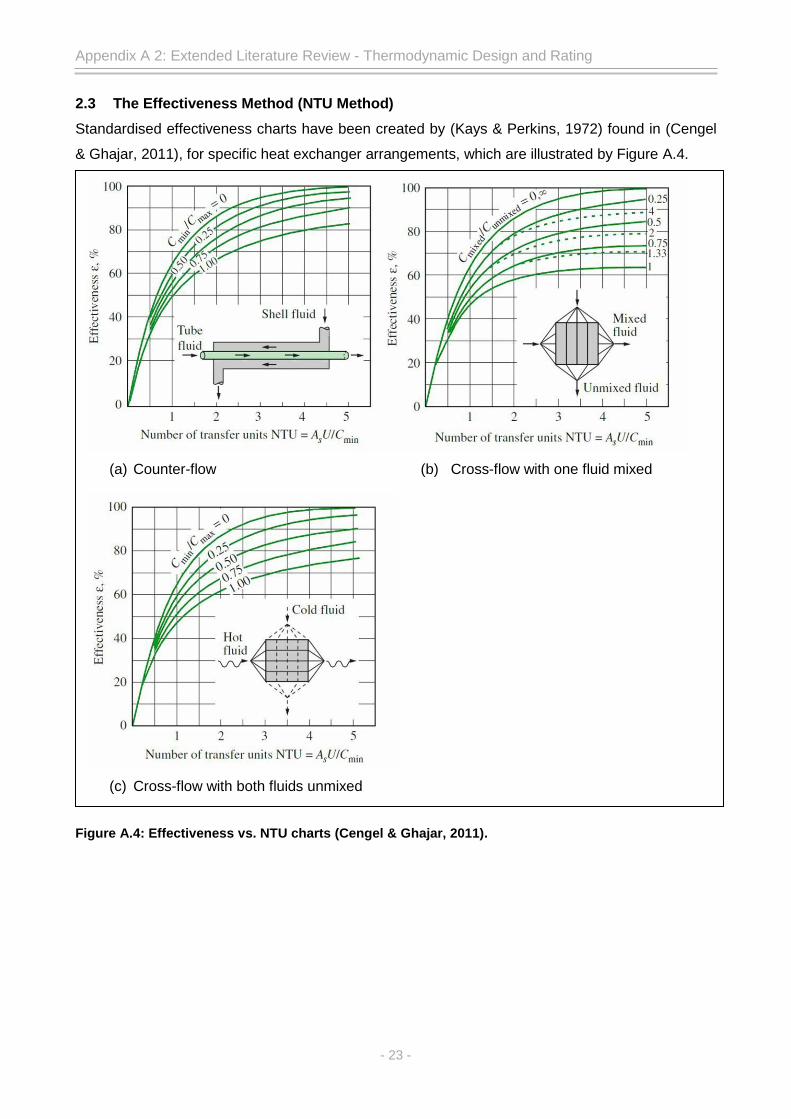
Appendix A 2: Extended Literature Review - Thermodynamic Design and Rating
- 23 -
2.3 The Effectiveness Method (NTU Method)
Standardised effectiveness charts have been created by (Kays & Perkins, 1972) found in (Cengel
& Ghajar, 2011), for specific heat exchanger arrangements, which are illustrated by Figure A.4.
Figure A.4: Effectiveness vs. NTU charts (Cengel & Ghajar, 2011).
(a) Counter-flow (b) Cross-flow with one fluid mixed
(c) Cross-flow with both fluids unmixed

Appendix A 2: Extended Literature Review - Thermodynamic Design and Rating
- 24 -
2.4 Shell Side Heat Transfer Coefficient
2.4.1 Boiling Regime – Nusselt Number Correlation
The experimental values of the surface fluid combination constant Csf and the fluid type constant n
is recorded in Table A.19, which is used in the calculation of nucleate boiling heat flux.
Table A.19: Experimental constants of surface-fluid combination (Cengel & Ghajar, 2011).
The geometry constant Ccr illustrated in Table A.20, is used in the calculation of the critical heat
flux and requires the calculation of the dimensionless parameter L*. The dimensionless parameter
is calculated with
Table A.20: Heater geometry constant (Cengel & Ghajar, 2011).
𝐿 𝐿 [𝑔(𝜌𝑙 𝜌𝑣)
𝜎]

Appendix A 2: Extended Literature Review - Thermodynamic Design and Rating
- 25 -
2.4.2 Reynolds Number Correlation for Flow over a Horizontal Tube
The dimensionless Reynolds number was derived by Osborne Reynolds (1842 – 1912). It is
essentially based on the ratio of inertia forces to viscous forces in a fluid (Cengel & Ghajar, 2011).
Reynolds number can be expressed for external flow as:
(A.39)
with u as the velocity of the fluid stream, and D the outer diameter of the tube.
Laminar flow occurs at low Reynolds numbers < 1000 and fully developed turbulent flow
occurs at Re = 2 x 10⁵, at namely, the critical Reynolds number (Recr). This, however, is dependent
on flow geometry, surface roughness and the level of fluctuations in the inlet stream (White, 2011).
2.4.3 Reynolds Number Correlation through Tube Bundles
The Reynolds number for flow through a tube bundle can be calculated for two scenarios of shell
and tube heat exchanger, namely, baffled or no baffle heat exchangers. If the heat exchanger has
no baffles, the heat transfer coefficient may be based on the equivalent diameter, De, where the
equivalent diameter is taken as four times the net flow area of the layout (tube pitch layout) divided
by the wetted perimeter:
(A.40)
(Kakaç & Liu, 2002) suggested a heat transfer correlation for shell side heat transfer of a baffle
less shell and tube heat exchanger as:
( )
(
)
(
)
(A.41)
with 2 x 10³ < (Res) < 1 x 10⁶
A new relation is introduced, Gs, the shell side mass velocity, which is the mass flow rate of
the shell side fluid divided by the bundle cross flow area (Acs). The equivalent diameter is
dependent on the pitch-tube layout, either square- or triangular-pitch layout. Thus, for the square
pitch the following equation is used to determine the equivalent diameter:
(
)
(A.42)
and for the triangular tube pitch:
( √
)
(A.43)

Appendix A 2: Extended Literature Review - Thermodynamic Design and Rating
- 26 -
Figure A.5 depicts a graphical representation of the pitch tube bundle layout, but more importantly
shows where the equivalent diameter lies (equivalent diameter lies within the hashed areas of
Figure A.5).
Figure A.5: Pitch tube layouts (Kakaç & Liu, 2002).
where the pitch size and clearance (C) are calculated with
( ) (A.44)
(A.45)
Heat exchangers that are baffled have the same set of equations, with a slight tweak to the bundle
cross flow area equation at the centre of the shell. Now, the baffle spacing (B) is added to the
equation, where conventionally the baffle spacing is set at 0.4 to 0.6 of the shell diameter.
(A.46)
Thus, the Reynolds number of baffled shell and tube heat exchangers can be calculated by using
the following equation extracted from (Kakaç & Liu, 2002):
(A.47)
2.5 Tube Side Heat Transfer Coefficient
Reynolds Number Correlation for Flow through Circular Ducts
The Reynolds number correlation for flow through a circular tube can be derived from the Reynolds
number correlation of external flow as
(A.48)
where Dh is the hydraulic diameter, which is equal to the inner diameter of the tube.

Appendix A 2: Extended Literature Review - Thermodynamic Design and Rating
- 27 -
(Kakaç & Liu, 2002) suggested the rearranging of Eq. A.48 and substituting velocity with a mass
flow rate relation yields a far simpler correlation for Reynolds number calculation as
(A.49)
The flow through a tube for most practical applications is laminar when Re < 2300,
turbulent when Re > 10 000, and in the transitional range for 2300 ≤ Re ≤ 10 000. It’s possible to
maintain laminar flow for Reynolds numbers above 2300 in very smooth tubes by avoiding tube
vibrations and flow disturbances (Cengel & Ghajar, 2011). In the transitional range of Reynolds
number the flow can switch between laminar and turbulent randomly.
2.6 Shell Side Pressure Drop
Pressure drops from the shell side depend on the geometrical layout of the shell and tube heat
exchanger, namely, the number of tubes in the tube bundle, and the baffle spacing and baffle cut.
Kern (1950) as found in (Kakaç & Liu, 2002) proposed that the pressure drop be a product of
friction factor f, the shell diameter Ds, the number of baffles Nb, and the mass velocity Gs, where
the equivalent diameter is calculated by Eq. A.32 & A.33. Thus, the pressure drop on the shell side
can be calculated using the following:
( )
(
⁄ )
(A.50)
The friction factor f is calculated with
( ( )) (A.51)
where (400 < Res < 106) The friction factor correlation for the shell has been tested based on data
obtained from actual heat exchangers, and takes entrance and exit losses into account (Kakaç &
Liu, 2002).
2.7 Tube Side Pressure Drop
The pressure drop of the tube side can be determined by knowing the number of tube passes, Np,
and the length of the tubes (L). The pressure drop for single tube pass heat exchanger can be
calculated using the following two equations, which were extracted from (Moody, 1994).
(A.52)

Appendix A 2: Extended Literature Review - Thermodynamic Design and Rating
- 28 -
(A.53)
The friction factor in the laminar region is calculated using
(A.54)
where the Reynolds number is limited to 2300.
2.8 Fouling Factor
The performance of a heat exchanger deteriorates with the course of its operation life as a result of
accumulating deposits or material corrosion. The extra layer of deposits represents additional
resistance from heat being transferred between the two fluids. The total effect of these
accumulations on the heat transfer is represented by a fouling factor Rf, which is a measure of
thermal resistance (Cengel & Ghajar, 2011).
In applications where fouling is likely to occur it should be considered in the thermodynamic
design and selection of the heat exchanger. In such applications where fouling is unavoidable, it
will be required that the total heat transfer surface area is increased by an over design percentage
to meet the heat transfer design requirements. Fouling factors are obviously zero for a new heat
exchanger, but with the course of operating time the performance slowly decreases. The fouling
factor depends on the operating temperature and fluid velocity, in other words fouling increases
with low fluid velocities and high fluid temperatures.
Thulukakanam (2000) proposed the overall heat transfer coefficient with fouling factors is
( )
(A.55)
Kakaç and Liu (2002) suggested that the over design percentage can be expressed by
(A.56)
with the total resistance factor and cleanliness factor as
(A.57)
(A.58)

- 29 -
3 MECHANICAL DESIGN RATING AND CONSIDERATIONS
Although, the main focus of this study is the thermodynamic design and rating of seven heat
exchangers for an aqua-ammonia absorption-desorption H&R cycle, the heat exchangers still need
to be manufactured and the mechanical rating still needs to be considered. Especially, since a
volatile refrigerant will be used under 10-to-14 times atmospheric pressure. Among the
considerations to be made are the thicknesses of the heat exchangers shells, the thicknesses of
the tubes in the tube bundle, the thicknesses of the tube sheets, and lastly the number of bolts for
the flanges of the connecting pipes.
First order stress calculations and standardised codes, such as ASME and TEMA, will be
used to determine whether the mechanical designs of the heat exchangers are deemed safe for
operation.
3.1 Tube Sheet Stress Calculations and TEMA Codes
The tube sheet of a fixed shell and tube heat exchanger plays an integral role of keeping the fluids
separate and containing the pressure to the inside of the heat exchanger. The minimum tube sheet
thickness can be determined by completing simple first order stress calculations from (Hibbeler,
2010) coupled with verification from the TEMA rule for tube sheet thicknesses (Thulukakanam,
2000). If the tube sheet is to be assumed as a circular disk with uniform loading, which is clamped
at its edges, the thickness can be calculated by a rearrangement of Eq. A.59 as
(A.59)
to
√
(A.60)
with PD as the effective design pressure, r as the radius of the tube sheet disk, and σallow as the
ASME allowable stress for the selected material. The TEMA rule for minimum tube sheet thickness
can be calculated using the following (Thulukakanam, 2000):
√
(A.61)
with

Appendix A 3: Literature Review - Mechanical Design Rating and Considerations
- 30 -
{
and
{
F is the parameter used to account for the restraint of the tube sheet; G is the diameter of the tube
sheet disk; and η is the TEMA ligament efficiency.
3.2 Tube Stress Calculations and ASME Codes
3.2.1 Thick Walled Cylinder
The thickness of the shell and of the tubes within each heat exchanger designs is highly important,
as the wall thickness is the only material separating the fluids from one another and the outside
environment. The outer shell of the heat exchanger can be viewed as a vessel, which experiences
internal pressure from the working fluids. When a vessel is under internal pressure then there are
stresses acting in on the wall of the vessel in the axial, radial, and circumferential direction, as
illustrated in Figure A.6 as available from (Engineeringtoolbox, 2015).
Figure A.6: Stress diagram of thick walled cylinders subjected to design pressure.
The following equations are derived from first order principles and can be used to
determine the stresses of a thick walled cylinder under pressure as
Axial stress:
(
)
(
) (A.62)
Hoop stress:
[(
)
(
)] [
( )
( (
))]
(A.63)

Appendix A 3: Literature Review - Mechanical Design Rating and Considerations
- 31 -
Radial stress:
[(
)
(
)] [
( )
( (
))]
(A.64)
Where:
Pi = the internal pressure;
Po = the external pressure;
ri = the inner radius of the shell;
ro = the outer radius of the shell;
r = mean radius of the shell;
A safety factor can be obtained from the stress calculations above by simply dividing by the
standardised allowable stress obtained from the ASME codes.
To verify the safety factor obtained from first principles, the ASME codes can be used to
determine the minimum thickness of the shell and tube walls. These codes are the industry
standard and used worldwide, where the equation for determining the minimum wall thickness
according to ASME B31.3 is
( ) (A.65)
where:
P = the internal gauge pressure;
Do = the outer diameter of the shell;
S = the allowable stress according to ASME pipe design tensile strength;
E = weld quality factor;
W = weld joint strength reduction factor;
Y = coefficient from Table 304.1.1 in ASME, 2014
The first order principles are used to determine a safety factor with standard sizes of pipes and
tubing, whereas the ASME wall thickness calculations act as confirmation that the standard pipe is
thick enough for the application.
(A.66)

Appendix A 3: Literature Review - Mechanical Design Rating and Considerations
- 32 -
3.2.2 Thin Walled Cylinder
Tubes are classified as thin walled cylinders when the wall thickness is approximately one tenth
the tubes radius. The stress calculations for thin walled cylinders are formulated to determine the
stresses of a pressure working on the inside of the cylinder.
Thin walled hoop stress:
(A.67)
Thin walled longitudinal stress:
(A.68)
To determine whether a tube wouldn’t collapse from pressure on the outside of the tube, a thick
walled analysis can be used as a conservative method of calculating the maximum stress and
comparing it to the allowable stress.
3.3 Header Bolt Calculations
The number of bolts needed to suitably fasten the headers and pipe flanges are calculated using
simple first principle equations obtained from (Budynas & Nisbett, 2011) with the internal pressure
acting on the end plate of the header, as illustrated by Figure A.7.
Figure A.7: Simplified heat exchanger header force diagram.
PD Tube
Bundle Ds
PD

Appendix A 3: Literature Review - Mechanical Design Rating and Considerations
- 33 -
The force exerted on the end plate of the header is calculated using the following:
(
) (A.69)
The force acting on the flange of the header due to the fasteners can be calculated using the
following:
(
) (A.70)
where Dflange is the outer diameter of the flange.
The operating force of the bolts are determined as
(A.71)
where Wflange is the width of the flange component.
The design force is a culmination of the operating force and the largest force between the
flange and end plate forces, where the design force is then used to determine the number of bolts
required as
(
) (A.72)
with:
σY = the yield strength of the bolt
Dbolt = the diameter of the bolt

- 34 -
4 OCCUPATIONAL HEALTH AND SAFETY OF AN AQUA-AMMONIA ABSORPTION-
DESORPTION CYCLE
The social, legal, health, safety, and environmental impact of products and designs have become
an important parameter to determine the success of a design in today’s day and age. Due to the
increasing demand for safer and cleaner designs, it is important to ensure that all legal aspects are
abided by, and that fatalities are not caused by the design product. This section will investigate the
social, legal, health, safety, and environmental impacts of the heat exchanger modules to be
designed.
4.1 Social and Legal Impacts
The physiological affects aqua-ammonia on humans are serious at high concentrations.
Refrigerant R717 becomes an explosive mixture in air between 20-30% mass concentration
(ANSI/ASHRAE, 1994). While South Africa seeks to finalise a SANS standard for ammonia as a
refrigerant under SANS 10400. A standard does not exist in South Africa, therefore, the design of
an aqua-ammonia absorption-desorption refrigeration plant will be designed according to the
United States of America’s Occupational Health and Safety Act for Process Safety Management
29CFR1910,119. This code provides comprehensive guidelines to designing and developing an
ammonia absorption refrigeration plant.
Codes and standards are also required when designing the mechanical components of the
aqua-ammonia absorption-desorption cycle. Since SANS 10400 is not yet in existence, the
structural design of the support mountings and welds for this project has been based on SANS
Code in (Parrot, 2005), and the module thickness based on design pressure accompanied by a
large safety factor. Sound levels are not a legal issue, as all the heat exchangers won’t be in close
proximity to people, but sound levels should be kept below 85 [dB].
4.2 Health Impacts
As it is now known that pure ammonia is a toxic substance, it can have different affects to the
human body at different levels of concentration when mixed with the air. At 100-200 ppm the eyes
start to feel agitated, when moving passed 500 ppm the human eye could have permanent. An
ammonia concentration of 5000 and above the human skin will attain second degree burns, at 400
ppm the human lunges will be agitated and start to blister, at 1700 ppm coughing will start and at
2400 ppm it becomes life threatening when inhaled (www.atsdr.cdc.gov, 2014).

Appendix A 4: Literature Review – Occupational Health and Safety
- 35 -
4.3 Safety Impacts
According to the Kyoto Protocol the safety requirements for designing an ammonia refrigeration
plant are that (29CFR1910.119, 1992):
All power to all circuits within of the absorption-desorption cycle should be automatically
shut-down should the ammonia reach 3% volume.
All circuits in which power should be maintained during high ammonia concentrations, for
instance the condenser, should have intrinsically safe fittings.
During maintenance of the several heat exchangers of the aqua-ammonia package unit would be
shut-down, during the inspection of the modules, as a safety precaution the licensed inspector
should wear the appropriate eye, mouth, and skin protection.
4.4 Environmental Impacts
Ammonia is an “environmentally friendly” refrigerant in other words ammonia is not contributing to
the depletion of the ozone layer (O3), greenhouse effect, or to global warming. Ammonia has a
very short atmospheric lifetime and therefore has no cumulative effect on the environment. It is
also known as a biodegradable substance. Ammonia is one of only few alternative refrigerants with
zero ODP (Ozone Depletion Potential) and zero GWP (Global Warming Potential) accepted by all
governments, ASHRAE, UNEP, International Institution of Refrigeration, and almost all Institutes of
Refrigeration worldwide (ANSI/ASHRAE, 1994).
Energy and efficiency of a system is highly important due to a lack of energy or high energy
demands. Energy in the form of mechanical work is normally much more expensive than in the
form of heat. Since the absorption-desorption H&R cycle uses less expensive thermal (heat)
energy, lower COP values are acceptable. Therefore, the aqua-ammonia absorption-desorption
H&R cycle is a viable alternative to the conventional energy thirsty vapour-compression cycle.

Appendix B
Extended Chapter 3 – Thermophysical Properties
Summary
Appendix B is mainly focused on the thermophysical properties of the thermodynamic states in the
aqua-ammonia absorption-desorption H&R cycle that have been excluded from the main body of
text. Some of the thermophysical property sample calculations of a thermodynamic state were
omitted due to the trivial nature of the sample calculation.

- i -
Table of Contents
1 EXTENDED THERMOPHYSICAL PROPERTIES ................................................................ B1
1.1 Thermophysical Properties of State 4 ............................................................................ B1
1.2 Thermophysical Properties of State 5 ............................................................................ B3
1.3 Thermophysical Properties of States 5 to 6 and 9 to 10 ................................................. B6
1.4 Thermophysical Properties of Weak and Strong Solution Aqua-Ammonia ..................... B9
1.5 Thermophysical Properties of Ethylene Glycol Water Mixtures .................................... B13
2 REMAINING THERMOPHYSICAL PROPERTIES OF STATE 3, 4, AND 5 ....................... B15
3 REMAINING THERMOPHYSICAL PROPERTIES STATE TP ........................................... B16
4 REMAINING THERMOPHYSICAL PROPERTIES STATE 6, 8, AND 10 ........................... B17
5 THERMOPHYSICAL PROPERTIES OF WEAK SOLUTION STATE 1, 2, AND 3 .............. B18
6 THERMOPHYSICAL PROPERTIES OF STRONG SOLUTION STATE 1 AND 2 .............. B19
List of Tables
Table B.1: Thermophysical properties of state 3, 4, and 5 for average ambient condition. .......... B15
Table B.2: Thermophysical properties of state 3, 4, and 5 for winter ambient condition............... B15
Table B.3: Thermophysical properties of state TP for average ambient condition. ...................... B16
Table B.4: Thermophysical properties of state TP for winter ambient condition. .......................... B16
Table B.5: Thermophysical properties of state 6, 8, & 10 for average ambient condition. ............ B17
Table B.6: Thermophysical properties of state 6, 8, & 10 for winter ambient condition. ............... B17
Table B.7: Thermophysical properties of weak solution state 1, 2, & 3 for summer ambient
condition. .................................................................................................................. B18
Table B.8: Thermophysical properties of weak solution state 1, 2, & 3 for average ambient
condition. .................................................................................................................. B18
Table B.9: Thermophysical properties of strong solution state 1 & 2 for summer ambient condition.
................................................................................................................................. B19
Table B.10: Thermophysical properties of strong solution state 1 & 2 for average ambient
condition. .................................................................................................................. B19
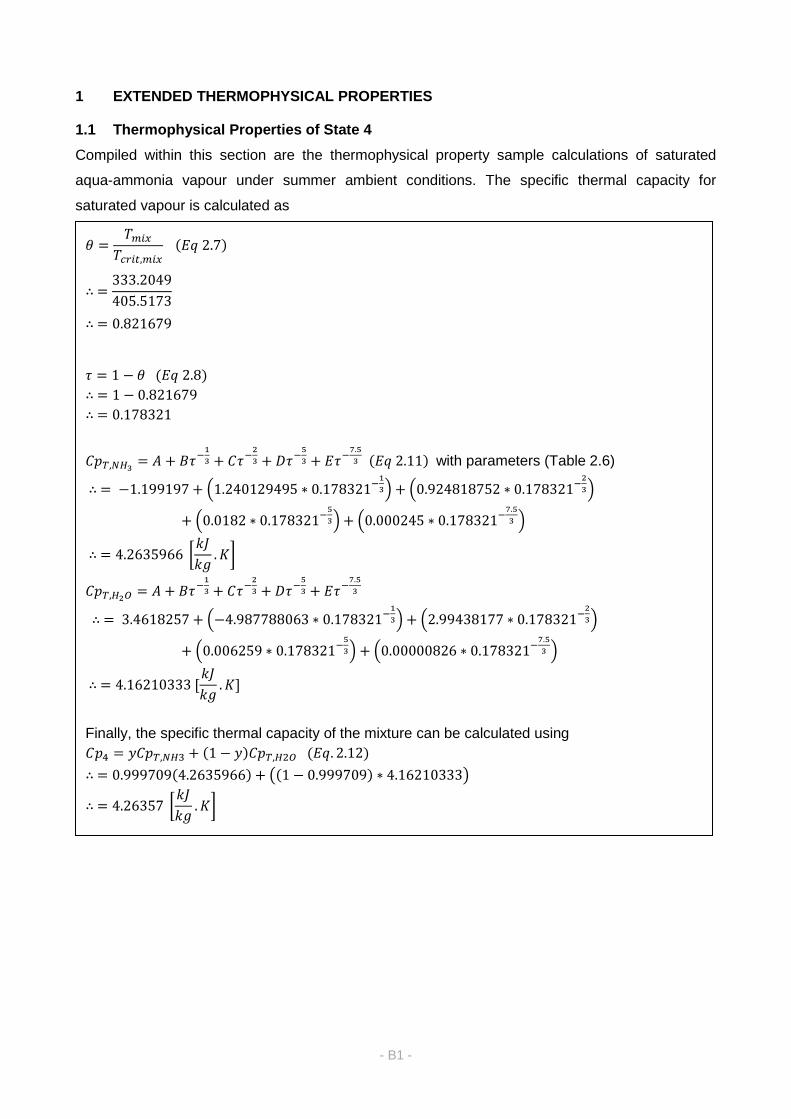
- B1 -
1 EXTENDED THERMOPHYSICAL PROPERTIES
1.1 Thermophysical Properties of State 4
Compiled within this section are the thermophysical property sample calculations of saturated
aqua-ammonia vapour under summer ambient conditions. The specific thermal capacity for
saturated vapour is calculated as
𝜃 =𝑇𝑚𝑖𝑥
𝑇𝑐𝑟𝑖𝑡,𝑚𝑖𝑥 𝐸𝑞 2.7
∴ =333.2049
405.5173
∴ = 0.821679
𝜏 = 1 − 𝜃 𝐸𝑞 2.8
∴ = 1 − 0.821679
∴ = 0.178321
∴ = −1.199197 + 1.240129495 ∗ 0.178321−1
3 + 0.924818752 ∗ 0.178321−2
3
+ 0.0182 ∗ 0.178321−5
3 + 0.000245 ∗ 0.178321−7.5
3
∴ = 4.2635966 𝑘𝐽
𝑘𝑔.𝐾
𝐶𝑝𝑇,𝐻2𝑂 = 𝐴 + 𝐵𝜏−1
3 + 𝐶𝜏−2
3 + 𝐷𝜏−5
3 + 𝐸𝜏−7.5
3
∴ = 3.4618257 + −4.987788063 ∗ 0.178321−1
3 + 2.99438177 ∗ 0.178321−2
3
+ 0.006259 ∗ 0.178321−5
3 + 0.00000826 ∗ 0.178321−7.5
3
∴ = 4.16210333 [𝑘𝐽
𝑘𝑔.𝐾]
𝐶𝑝4 = 𝑦𝐶𝑝𝑇,𝑁𝐻3 + 1 − 𝑦 𝐶𝑝𝑇,𝐻2𝑂 𝐸𝑞. 2.12
∴ = 0.999709 4.2635966 + 1 − 0.999709 ∗ 4.16210333
∴ = 4.26357 𝑘𝐽
𝑘𝑔.𝐾
𝐶𝑝𝑇,𝑁𝐻3 = 𝐴 + 𝐵𝜏−1
3 + 𝐶𝜏−2
3 + 𝐷𝜏−5
3 + 𝐸𝜏−7.5
3 𝐸𝑞 2.11 with parameters (Table 2.6)
Finally, the specific thermal capacity of the mixture can be calculated using

Appendix B 1: Extended Thermophysical Properties
- B2 -
The density of saturated vapour state 4 is determined as
The dynamic viscosity of saturated vapour of state 4 (summer design conditions) are:
∴ = 11.118577 𝑘𝑔
𝑚3
∴ = 0.7579289 𝑘𝑔
𝑚3
𝜌𝑁𝐻3,𝑇𝑁𝐻3 = 7.3313701 𝑘𝑔
𝑚3 𝑎𝑛𝑑 𝜌𝐻2𝑂,𝑇𝐻2𝑂 = 7.7712887 𝑘𝑔
𝑚3
𝜌4 = 𝑦𝜌𝑁𝐻3,𝑇𝑁𝐻3 + 1 − 𝑦 𝜌𝐻2𝑂,𝑇𝐻2𝑂 + ∆𝜌𝑇𝑚,𝑥
∗
∴ = 0.999709 ∗ 7.3313701 + 1 − 0.999709 ∗ 7.17712887 + 0.7579289
∴ = 8.08943 𝑘𝑔
𝑚3
∆𝜌𝑚𝑎𝑥,𝑇𝑚 = 𝑒𝐽−𝐾/𝑇𝑚∗ with parameters Table 2.8
∆𝜌𝑇𝑚,𝑥
∗ = 𝐴 1 − 𝑦 𝐵 1 − 𝑒𝐶𝑦𝐷 ∆𝜌𝑚𝑎𝑥,𝑇𝑚 𝐸𝑞 2.18 with parameters Table 2.8
Using Eq. 2.19 and parameters set in Table 2.9 the densities of pure ammonia and water are
calculated as
Substituting the above values into Eq. 2.17 yields the density of the aqueous ammonia mixture.
∴ = 0.8472279
𝜑21 = 𝜑21𝜇𝐻2𝑂
𝜇𝑁𝐻3
𝑀𝑁𝐻3
𝑀𝐻2𝑂
∴ = 1.2009746
𝜇4 =𝑦𝜇𝑁𝐻3
𝑦 + 1 − 𝑦 𝜑12+
1 − 𝑦 𝜇𝐻2𝑂 1 − 𝑦 + 𝑦𝜑21
∴ = 0.999709 ∗ 1.18881𝐸 −05
0.999709 + 1 − 0.999709 ∗ 0.8472279+ 1 − 0.999709 ∗ 1.78265𝐸 −05
1 − 0.999709 ∗ 1.2009746
∴ = 1.188948𝐸 − 05 𝑘𝑔
𝑚. 𝑠
𝜑12 = 1+
𝜇𝑁𝐻3𝜇𝐻2𝑂
0.5
𝑀𝐻2𝑂𝑀𝑁𝐻3
0.25
2
8 1+𝑀𝑁𝐻3𝑀𝐻2𝑂
0.5 𝐸𝑞 2.22 ,where μNH3 = 1.18881(-05) kg/m.s and
μH2O = 1.78265E(-05) kg/m.s

Appendix B 1: Extended Thermophysical Properties
- B3 -
The thermal conductivity of state 4 is determined using similar equation to dynamic viscosity, only
exception is the substituting of values of thermal conductivity for pure ammonia and water.
Lastly, the Prandtl number for state 4 is calculated using the values of Cp,4, μ4, and k4.
1.2 Thermophysical Properties of State 5
Compiled within this section are the thermophysical property sample calculations of saturated
aqua-ammonia liquid under summer ambient conditions. The specific thermal capacity of state 5
can be calculated as
𝜑21 = 𝜑21𝑘𝐻2𝑂
𝑘𝑁𝐻3
𝑀𝑁𝐻3
𝑀𝐻2𝑂
∴ = 1.232643
𝑘4 =𝑦𝑘𝑁𝐻3
𝑦 + 1 − 𝑦 𝜑12+
1 − 𝑦 𝑘𝐻2𝑂 1 − 𝑦 + 𝑦𝜑21
∴ = 0.999709 ∗ 0.0341093
0.999709 + 1 − 0.999709 ∗ 0.829371+ 1 − 0.999709 ∗ 0.0536266
1 − 0.999709 ∗ 1.232643
∴ = 0.034114 𝑊
𝑚.𝐾
𝜑12 = 1+
𝑘𝑁𝐻3𝑘𝐻2𝑂
0.5
𝑀𝐻2𝑂𝑀𝑁𝐻3
0.25
2
8 1+𝑀𝑁𝐻3𝑀𝐻2𝑂
0.5 𝐸𝑞 2.24 ,where kNH3 = 0.0341093 W/m.K and
kH2O = 0.0536266 W/m.K
∴ = 0.829371
𝑃𝑟4 =𝜇𝑚𝑖𝑥𝐶𝑝𝑚𝑖𝑥
𝑘𝑚𝑖𝑥 𝐸𝑞. 2.25
∴ =4.26258 ∗ 103 ∗ 1.188948𝐸 − 05
0.034114
∴ = 1.485959 [-]
𝜃 =𝑇𝑚𝑖𝑥
𝑇𝑐𝑟𝑖𝑡,𝑚𝑖𝑥 𝐸𝑞 2.7
∴ =296.15
408.86745
∴ = 0.724318
𝜏 = 1 − 𝜃 𝐸𝑞 2.8
∴ = 1 − 0.724318
∴ = 0.275682

Appendix B 1: Extended Thermophysical Properties
- B4 -
The density of saturated liquid state 5 can be calculated as
Substituting the above values into Eq. 2.13 yields the density of the aqueous ammonia mixture.
Dynamic viscosity for saturated liquid of state 5 can be approximated as
∴ = 3.875648 + 0.242125 ∗ 0.275682−1
∴ = 4.753924 𝑘𝐽
𝑘𝑔.𝐾
∴ = 3.665785 + 0.236312 ∗ 0.275682−1
∴ = 4.522975 [𝑘𝐽
𝑘𝑔.𝐾]
𝐶𝑝5 = 𝑥𝐶𝑝𝑇,𝑁𝐻3 + 1 − 𝑥 𝐶𝑝𝑇,𝐻2𝑂 𝐸𝑞. 2.10
∴ = 0.99 4.753924 + 1 − 0.99 ∗ 4.522975
∴ = 4.75161 𝑘𝐽
𝑘𝑔.𝐾
𝐶𝑝𝑇,𝑁𝐻3 = 𝐴𝑐𝑝 + 𝐵𝑐𝑝 ∗ 𝜏−1 𝐸𝑞 2.9 with parameters (Table 2.5)
𝐶𝑝𝑇,𝐻2𝑂 = 𝐴𝑐𝑝 + 𝐵𝑐𝑝 ∗ 𝜏−1 𝐸𝑞 2.9 with parameters (Table 2.5)
Now, the specific thermal capacity of the mixture can be calculated using
∆𝜌𝑇𝑚,𝑥
∗ = [𝑥 1 − 𝑥 − 𝐴𝑥2 1 − 𝑥 ] ∗ 𝜌𝑁𝐻3,𝑇𝑁𝐻30.5 ∗ 𝜌𝐻2𝑂,𝑇𝐻2𝑂
0.5 𝐸𝑞. 2.14
∴ = [0.99 1 − 0.99 − 1.1499893 0.992 1 − 0.99 ] 609.4770.5 ∗ 869.6420.5
∴ = −0.998161 𝑘𝑔
𝑚3 𝑒𝑥𝑐𝑒𝑠𝑠
Where variable A is determined using Eqs. 2.15 & 2.16, Table 2.7, and ρNH3 = 609.477 [kg/m3]
and ρH2O = 869.642 [kg/m3]
𝜌5 = 𝑥 𝜌𝑁𝐻3,𝑇𝑁𝐻3 + 1 − 𝑥 𝜌𝐻2𝑂,𝑇𝐻2𝑂 + ∆𝜌𝑇𝑚,𝑥
∗
∴ = 0.99 ∗ 609.477 + 1 − 0.99 ∗ 869.642 − 0.998161
∴ = 611.081 𝑘𝑔
𝑚3
𝐹 𝑥 = 6.38 1 − 𝑥 1.125𝑥 1 − 𝑒−0.585𝑥 1−𝑥 0.18
ln 𝜇𝑁𝐻30.5 ∗ 𝜇𝐻2𝑂
0.5
∴ = −0.074496 𝑘𝑔
𝑚. 𝑠
Where the values of μNH3 = 0.0001519 [kg/m.s] and μH2O = 0.000142 [kg/m.s] are determined
via linear interpolation as a function of substance temperature.

Appendix B 1: Extended Thermophysical Properties
- B5 -
Thermal conductivity of state 5 saturated liquid:
Lastly, the Prandtl number for state 5 is calculated using the values of Cp, μ, and k.
∆𝜇 𝑇𝑚𝑖𝑥 ,𝑥 = 0.534 − 0.815 𝑇𝑚
𝑇𝑐,𝐻2𝑂 ∗ 𝐹 𝑥 𝐸𝑞. 2.21
∴ = 0.534 − 0.815 296.15
647.14 ∗ −0.074496
∴ = −0.011996304 𝑘𝑔
𝑚. 𝑠
𝑙𝑛 𝜇5 = 𝑥 𝑙𝑛 𝜇𝑁𝐻3,𝑇𝑁𝐻3 + 1 − 𝑥 𝑙𝑛 𝜇𝐻2𝑂,𝑇𝐻2𝑂 + ∆𝜇 𝑇𝑚𝑖𝑥 ,𝑥
∴ = 0.99 ln 0.0001519 + 1 − 0.99 ln 0.000142 − 0.011996304
∴ ln 𝜇5 = −8.804958
∴ = 0.000149988 𝑘𝑔
𝑚. 𝑠
Using Eq. 2.20 and substituting for the value of excess dynamic viscosity, the saturated liquid
dynamic viscosity is obtained as
∴ = 610.3259 0.990.425
∴ = 607.725 𝑘𝑔
𝑚3
𝑘5 = 𝑥 𝑘𝑁𝐻3 𝜌𝑁𝐻3+ + 1 − 𝑥 𝑘𝐻2𝑂 𝑇𝐻2𝑂
∴ = 0.99 ∗ 0.48749 + 1 − 0.99 ∗ 0.669
∴ = 0.48931 𝑊
𝑚.𝐾
𝜌𝑁𝐻3+ = 𝜌𝑁𝐻3 𝑇𝑁𝐻3 𝑥
0.425 ,where ρNH3 = 610.3259 [kg/m3]
The thermal conductivity of pure ammonia is a function of density and has been determined via
linear interpolation as kNH3(ρNH3) = 0.48749 [W/m.K], and for water as a function of temperature
kH2O = 0.669 [W/m.K].
Substituting the above values into Eq. 2.23 yields the thermal conductivity of the aqueous
ammonia mixture.
𝑃𝑟5 =𝜇𝑚𝑖𝑥𝐶𝑝𝑚𝑖𝑥
𝑘𝑚𝑖𝑥 𝐸𝑞 2.25
∴ =4.75161 ∗ 103 ∗ 0.000149988
0.48931
∴ = 1.4561 [-]

Appendix B 1: Extended Thermophysical Properties
- B6 -
1.3 Thermophysical Properties of States 5 to 6 and 9 to 10
This section focuses on the thermophysical properties of the inlet and outlet conditions of the pre-
cool heat exchanger control volume for state 5 to 6 and 9 to 10, as depicted in Figures 3.1 and 3.3.
Enthalpy of State 5 to 6
The enthalpy values of state 5 are already known as previously calculated in Chapter 3.1.2, though
the enthalpy of state 6 is to be determined. EES can provide with the enthalpy values for sub-
cooled liquid aqua-ammonia, but for purposes of consistency the mathematical method is used to
determine the enthalpy of state 6. Using Eq. 2.3 and equation parameters in Table A.3, the
enthalpy of state 6 is calculated as
The temperatures of state 6 for the three ambient conditions were obtained from the MS Excel
‘Clear Sky’ data sheet in Appendix D 2.1.
Now, that the enthalpy values of state 6 have been calculated it is possible to determine the
heat transfer rate of the sub-cooled liquid line of aqueous ammonia.
Winter design conditions:
Average design conditions:
𝛼6,𝑊𝑅𝑇 270.141, 0.99 = − 25.8159 𝑘𝐽
𝑘𝑔
𝛼6,𝐷𝑆𝑁 276.386, 0.99 = 3.00148 𝑘𝐽
𝑘𝑔
𝛼6,𝑆𝑀𝑅 281.503, 0.99 = 26.8503 𝑘𝐽
𝑘𝑔
𝑄 𝑃𝐶,𝑊𝑅𝑇 = 𝑚 6,𝑊𝑅𝑇 𝛼6,𝑊𝑅𝑇 − 𝛼5,𝑊𝑅𝑇 𝐸𝑞. 2.27
∴ = 0.000539 −25.8159 − 11.1974
∴ = 19.9502 𝑊 𝐻𝑒𝑎𝑡 𝑅𝑒𝑚𝑜𝑣𝑒𝑑
𝑄 𝑃𝐶,𝐷𝑆𝑁 = 𝑚 6,𝐷𝑆𝑁 𝛼6,𝐷𝑆𝑁 − 𝛼5,𝐷𝑆𝑁 𝐸𝑞. 2.27
∴ = 0.0005816 3.00148 − 58.1984
∴ = 32.1026 𝑊 𝐻𝑒𝑎𝑡 𝑅𝑒𝑚𝑜𝑣𝑒𝑑

Appendix B 1: Extended Thermophysical Properties
- B7 -
Summer design conditions:
Therefore, for state 5 to 6, it is clear that summer conditions has the highest heat transfer rate and
should yield the largest heat transfer surface area when calculating the thermodynamic design
sizing. Thus, in this oeuvre, the summer condition thermophysical properties of state 6 will be
calculated and illustrated in below, and the remaining conditions thermophysical properties are
added to section 4 of Appendix B.
The temperature of state 10 is unknown and can be calculated by an energy balance
between state 5 to 6 and 9 to 10.
The temperature of state 10 can be determined via EES’ temperature function for pure ammonia
by substituting the variables of pressure and enthalpy (P10 = 236.2 kPa, α10 = 1515.3292 kJ/kg).
State 6 Thermophysical Properties
The sub-cooled liquid phase of state 6 is determined by means of the mathematical method set out
in Chapter 2.4.1 for saturated liquid. As a liquid is incompressible the values obtained by
mathematical method are within good accordance to EES’ thermophysical properties. Thus, the
thermophysical properties of state 6 under summer ambient conditions, with temperature and
pressure at 8.353 °C and 939.54 [kPa], respectively, are:
𝑄 𝑃𝐶,𝑆𝑀𝑅 = 𝑚 6,𝑆𝑀𝑅 𝛼6,𝑆𝑀𝑅 − 𝛼5,𝑆𝑀𝑅 𝐸𝑞. 2.27
∴ = 0.0006129 26.8503 − 96.5153
∴ = 42.6977 𝑊 𝐻𝑒𝑎𝑡 𝑅𝑒𝑚𝑜𝑣𝑒𝑑
𝑄 𝑖𝑛 = 𝑄 𝑜𝑢𝑡
𝑄 𝑃𝐶,𝑆𝑀𝑅 = 𝑚 9,𝑆𝑀𝑅 𝛼10,𝑆𝑀𝑅 − 𝛼9,𝑆𝑀𝑅 𝐸𝑞. 2.27
∴ 42.6977 = 0.0005986 𝛼10,𝑆𝑀𝑅 − 1444 ∗ 103
∴ 𝛼10,𝑆𝑀𝑅 = 1515.3292 𝑘𝐽
𝑘𝑔
𝑇10,𝑆𝑀𝑅 236.2, 1515.3292 = 15.11 [°𝐶]

Appendix B 1: Extended Thermophysical Properties
- B8 -
State 9 Thermophysical Properties
As depicted by Figure 3.1, state 9 is at the saturated vapour state of pure ammonia, this is due to a
tertiary gas in the evaporator module which creates a partial pressure of the aqua-ammonia
mixture. The partial pressure of aqua-ammonia assists the evaporation process whereby pure
ammonia can evaporate first out of the mixture, thus, creating the pure ammonia saturated vapour
state 9. As state 9 and 10 consists of pure ammonia vapour the thermophysical properties are
determined by use of EES’ property call function. Under state 9, the thermophysical properties are
determined as a function of pressure and quality for summer ambient conditions. The partial
pressure of 236.2 [kPa] is desired for all ambient design conditions, thus the thermophysical
properties of state 9 are valid for winter, average, and summer design conditions.
State 10 Thermophysical Properties
The transport properties of superheated state 10 are obtained by using EES’ property call function,
with input parameters of pressure and enthalpy. The remaining thermophysical properties of winter
and average design conditions are available in section 4.
𝐶𝑝6 = 4.6506 𝑘𝐽
𝑘𝑔
𝜌6 = 632.288 𝑘𝑔
𝑚3
𝜇6 = 0.000176853 𝑘𝑔
𝑚. 𝑠
𝑘6 = 0.52233 𝑊
𝑚.𝐾
𝑃𝑟6 = 1.5746[−]
𝐶𝑝9 236.2, 1.00 = 2.481 𝑘𝐽
𝑘𝑔
𝜌9 236.2, 1.00 = 1.966 𝑘𝑔
𝑚3
𝜇9 236.2, 1.00 = 0.0000086 𝑘𝑔
𝑚. 𝑠
𝑘9 236.2, 1.00 = 0.02212 𝑊
𝑚.𝐾
𝑃𝑟9 236.2, 1.00 = 0.9645 [−]

Appendix B 1: Extended Thermophysical Properties
- B9 -
1.4 Thermophysical Properties of Weak and Strong Aqua-Ammonia Solutions
The enthalpy values of the strong aqua-ammonia solution can be determined by means of the
mathematical method, but the thermophysical properties of the weak aqua-ammonia solution can’t
be calculated using the mathematical method proposed in (Conde-Petit, 2004). Thus, it was
decided that for purposes of the design continuity for the regenerative and auxiliary heat
exchangers the thermophysical properties will be calculated using EES’ property call function. This
does create a problem for the strong solution’s transport properties out of the regenerative heat
exchanger as the fluid is in a two-phase state at its outlet. The quality is low enough that a
conservative assumption can be made for the values of the thermophysical properties. It’s
therefore assumed that the thermophysical properties of the outlet of strong solution be calculated
at Q = 0.00. In other words the properties of dynamic viscosity and thermal conductivity are
calculated at saturated liquid for the strong aqua-ammonia solution.
But first the values of enthalpy for the strong solution’s in and outlet conditions are
determined with EES, where enthalpy requires three input parameters: pressure, mixture
temperature, and mass concentration.
𝐶𝑝10 236.2, 1515.3292 = 2.294 𝑘𝐽
𝑘𝑔
𝜌10 236.2, 1515.3292 = 1.728 𝑘𝑔
𝑚3
𝜇10 236.2, 1515.3292 = 9.689𝐸 −06 𝑘𝑔
𝑚. 𝑠
𝑘10 236.2, 1515.3292 = 0.02425 𝑊
𝑚.𝐾
𝑃𝑟10 236.2, 1515.3292 = 0.9167 [−]
𝛼𝑠𝑠,𝑖𝑛,𝑊𝑅𝑇 515.84, 33.223, 0.4523 = −69.03 𝑘𝐽
𝑘𝑔
𝛼𝑠𝑠,𝑖𝑛,𝐷𝑆𝑁 727.25, 54.024, 0.453 = 3.968 𝑘𝐽
𝑘𝑔
𝛼𝑠𝑠,𝑖𝑛,𝑆𝑀𝑅 939.54, 68.234, 0.4556 = 68.12 𝑘𝐽
𝑘𝑔

Appendix B 1: Extended Thermophysical Properties
- B10 -
Energy Balance of Regenerative Heat Exchanger
Using the mass flow rates obtained from the MS Excel ‘Clear Sky’ data sheet in Appendix D 8.1
and the enthalpy values obtained above, the heat transfer rate of the regenerative heat exchanger
can be calculated.
Winter design conditions:
Average design conditions:
Summer design conditions:
It’s clear that for winter design conditions the heat transfer rate has the highest output and would
require the largest surface area. Thus, the thermophysical properties of the regenerative heat
exchanger can be calculated for winter design conditions and implemented in the thermodynamic
design of Chapter 4.
The only unknown at the regenerative heat exchanger is the outlet conditions of the weak
solution, whereby the temperature of (ws, out) can be calculated by means of an energy balance
determining the enthalpy of state (ws, out).
𝛼𝑠𝑠,𝑜𝑢𝑡,𝑊𝑅𝑇 515.84, 49.55, 0.4523 = −3.824 𝑘𝐽
𝑘𝑔 𝑤𝑖𝑡ℎ 𝑄 = 0.008374
𝛼𝑠𝑠,𝑜𝑢𝑡,𝐷𝑆𝑁 727.25, 61.46, 0.453 = 56.07 𝑘𝐽
𝑘𝑔 𝑤𝑖𝑡ℎ 𝑄 = 0.01341
𝛼𝑠𝑠,𝑜𝑢𝑡,𝑆𝑀𝑅 939.54, 70.8, 0.4556 = 102 𝑘𝐽
𝑘𝑔 𝑤𝑖𝑡ℎ 𝑄 = 0.01593
𝑄 𝑅𝐸𝐺𝐸𝑁,𝑊𝑅𝑇 = 𝑚 𝑠𝑠,𝑊𝑅𝑇 𝛼𝑠𝑠,𝑜𝑢𝑡,𝑊𝑅𝑇 − 𝛼𝑠𝑠,𝑖𝑛,𝑊𝑅𝑇 𝐸𝑞. 2.26
∴ = 0.0044974 −3.824 − −69.03
∴ = 293.2575 𝑊 𝐻𝑒𝑎𝑡 𝐴𝑑𝑑𝑒𝑑
𝑄 𝑅𝐸𝐺𝐸𝑁,𝐷𝑆𝑁 = 𝑚 𝑠𝑠,𝐷𝑆𝑁 𝛼𝑠𝑠,𝑜𝑢𝑡,𝐷𝑆𝑁 − 𝛼𝑠𝑠,𝑖𝑛,𝐷𝑆𝑁 𝐸𝑞. 2.26
∴ = 0.0036046 102 − 68.12
∴ = 122.1238 𝑊 𝐻𝑒𝑎𝑡 𝐴𝑑𝑑𝑒𝑑
𝑄 𝑅𝐸𝐺𝐸𝑁,𝑆𝑀𝑅 = 𝑚 𝑠𝑠,𝑆𝑀𝑅 𝛼𝑠𝑠,𝑜𝑢𝑡,𝑆𝑀𝑅 − 𝛼𝑠𝑠,𝑖𝑛,𝑆𝑀𝑅 𝐸𝑞. 2.26
∴ = 0.003879 56.07 − 3.968
∴ = 202.1037 𝑊 𝐻𝑒𝑎𝑡 𝐴𝑑𝑑𝑒𝑑
∴ 𝛼𝑤𝑠,𝑜𝑢𝑡,𝑊𝑅𝑇 = −23.3697 𝑘𝐽
𝑘𝑔
𝑄 𝑅𝐸𝐺𝐸𝑁,𝑊𝑅𝑇 = 𝑚 𝑤𝑠,𝑊𝑅𝑇 𝛼𝑤𝑠,𝑜𝑢𝑡,𝑊𝑅𝑇 − 𝛼𝑤𝑠,𝑖𝑛,𝑊𝑅𝑇 𝐸𝑞. 2.26
∴ 293.2575 = 0.003971 𝛼𝑤𝑠,𝑜𝑢𝑡,𝑊𝑅𝑇 − 50.48

Appendix B 1: Extended Thermophysical Properties
- B11 -
Energy Balance of the Auxiliary Heat Exchanger
The heat transfer rates of the auxiliary heat exchanger can be calculated as
Winter design condition:
Average design condition:
Summer design conditions:
Though the values of heat transfer rate are larger for summer and average design conditions, the
winter design condition has a larger mass flow rate at a lower operating pressure, which will result
in a larger heat transfer surface area.
Weak Solution Thermophysical Properties
The transport properties of the weak solutions fluid states were determined by using EES’ property
call function for aqueous ammonia, where the input parameters are: pressure, temperature in [°C],
and mass concentration. The remaining design conditions’ properties are added to section 5 of
Appendix B.
Weak solution state 1:
∴ = 608.834 𝑊 𝐻𝑒𝑎𝑡 𝑅𝑒𝑚𝑜𝑣𝑒𝑑
𝑄 𝐴𝑈𝑋,𝑊𝑅𝑇 = 𝑚 𝑤𝑠,𝑊𝑅𝑇 𝛼𝑤𝑠,3,𝑊𝑅𝑇 − 𝛼𝑤𝑠,2,𝑊𝑅𝑇 𝐸𝑞. 2.26
∴ = 0.003971 −176.7 − −23.38
∴ = 710.044 𝑊 𝐻𝑒𝑎𝑡 𝑅𝑒𝑚𝑜𝑣𝑒𝑑
𝑄 𝐴𝑈𝑋,𝐷𝑆𝑁 = 𝑚 𝑤𝑠,𝐷𝑆𝑁 𝛼𝑤𝑠,3,𝐷𝑆𝑁 − 𝛼𝑤𝑠,2,𝐷𝑆𝑁 𝐸𝑞. 2.26
∴ = 0.003311 −148.5 − 65.95
∴ = 767.432 𝑊 𝐻𝑒𝑎𝑡 𝑅𝑒𝑚𝑜𝑣𝑒𝑑
𝑄 𝐴𝑈𝑋,𝑆𝑀𝑅 = 𝑚 𝑤𝑠,𝑆𝑀𝑅 𝛼𝑤𝑠,3,𝑆𝑀𝑅 − 𝛼𝑤𝑠,2,𝑆𝑀𝑅 𝐸𝑞. 2.26
∴ = 0.003006 −109.1 − 146.2
𝐶𝑝𝑤𝑠,1,𝑊𝑅𝑇 515.84, 61.72, 0.378 = 4.31478 𝑘𝐽
𝑘𝑔.𝐾 𝐸𝑞 2.10
𝜌𝑤𝑠,1,𝑊𝑅𝑇 515.84, 61.72, 0.378 = 840.9 𝑘𝑔
𝑚3
𝜇𝑤𝑠,1,𝑊𝑅𝑇 515.84, 61.72, 0.378 = 0.0004314 𝑘𝑔
𝑚. 𝑠
𝑘𝑤𝑠,1,𝑊𝑅𝑇 515.84, 61.72, 0.378 = 0.51 𝑊
𝑚.𝐾
𝑃𝑟𝑤𝑠,1,𝑊𝑅𝑇 515.84, 61.72, 0.378 = 3.6498[−] 𝐸𝑞 2.25

Appendix B 1: Extended Thermophysical Properties
- B12 -
Weak solution state 2:
Weak solution state 3:
Strong Solution Thermophysical Properties
The strong aqua-ammonia solution’s thermophysical properties are approximated using the input
parameters of: pressure, temperature, and mass concentration into EES’ property call function.
Strong solution state 1:
𝐶𝑝𝑤𝑠,2,𝑊𝑅𝑇 515.84, 44.94, 0.378 = 4.2777 𝑘𝐽
𝑘𝑔.𝐾 𝐸𝑞 2.10
𝜌𝑤𝑠,2,𝑊𝑅𝑇 515.84, 44.94, 0.378 = 855.7 𝑘𝑔
𝑚3
𝜇𝑤𝑠,2,𝑊𝑅𝑇 515.84, 44.94, 0.378 = 0.0006301 𝑘𝑔
𝑚. 𝑠
𝑘𝑤𝑠,2,𝑊𝑅𝑇 515.84, 44.94, 0.378 = 0.4406 𝑊
𝑚.𝐾
𝑃𝑟𝑤𝑠,2,𝑊𝑅𝑇 515.84, 44.94, 0.378 = 6.1176[−] 𝐸𝑞 2.25
𝐶𝑝𝑤𝑠,3,𝑊𝑅𝑇 515.84, 5, 0.378 = 4.20632 𝑘𝐽
𝑘𝑔.𝐾 𝐸𝑞 2.10
𝜌𝑤𝑠,3,𝑊𝑅𝑇 515.84, 5, 0.378 = 875.2 𝑘𝑔
𝑚3
𝜇𝑤𝑠,3,𝑊𝑅𝑇 515.84, 5, 0.378 = 0.001636 𝑘𝑔
𝑚. 𝑠
𝑘𝑤𝑠,3,𝑊𝑅𝑇 515.84, 5, 0.378 = 0.4899 𝑊
𝑚.𝐾
𝑃𝑟𝑤𝑠,3,𝑊𝑅𝑇 515.84, 5, 0.378 = 14.047[−] 𝐸𝑞 2.25
𝐶𝑝𝑠𝑠,1,𝑊𝑅𝑇 515.84, 33.223, 0.4523 = 4.2876 𝑘𝐽
𝑘𝑔.𝐾 𝐸𝑞 2.10
𝜌𝑠𝑠,1,𝑊𝑅𝑇 515.84, 33.223, 0.4523 = 870.3 𝑘𝑔
𝑚3
𝜇𝑠𝑠,1,𝑊𝑅𝑇 515.84, 33.223, 0.4523 = 0.0008615 𝑘𝑔
𝑚. 𝑠
𝑘𝑠𝑠,1,𝑊𝑅𝑇 515.84, 33.223, 0.4523 = 0.4321 𝑊
𝑚.𝐾
𝑃𝑟𝑠𝑠,1,𝑊𝑅𝑇 515.84, 33.223, 0.4523 = 8.5484[−] 𝐸𝑞 2.25

Appendix B 1: Extended Thermophysical Properties
- B13 -
Strong solution state 2:
1.5 Thermophysical Properties of Ethylene Glycol Water Mixtures
Ethylene glycol water solution acts as the secondary refrigerant or coolant of the absorption-
desorption cycle, and the calculation of the thermophysical properties of ethylene glycol water
mixture is constant throughout the design process. Therefore, the calculation of the thermophysical
properties will only be demonstrated once for the coolant inlet and outlet of the auxiliary heat
exchanger. The inlet temperature has been pre-determined as the coolant comes from the
absorber module. The outlet temperature is an iterative estimation, which influences the efficiency
of the heat exchanger. Thus, if the efficiency is to low the outlet temperature is adjusted
accordingly. The thermophysical properties of the coolant is determined at the fluid bulk
temperature and mass concentration of ethylene glycol in water, thus, for the conditions of:
Tclnt,bulk,WRT = 21.7275 [°C] or 294.8775 [K] and x = 0.25. Thus, the thermophysical properties are:
𝐶𝑝𝑠𝑠,2,𝑊𝑅𝑇 515.84, 49.55, 0.4523 = 4.3238 𝑘𝐽
𝑘𝑔.𝐾 𝐸𝑞 2.10
𝜌𝑠𝑠,2,𝑊𝑅𝑇 515.84, 49.55, 0.4523 = 274.7 𝑘𝑔
𝑚3
𝜇𝑠𝑠,2,𝑊𝑅𝑇 515.84, 49.55,𝑄 = 0 = 0.0005241 𝑘𝑔
𝑚. 𝑠
𝑘𝑠𝑠,2,𝑊𝑅𝑇 515.84, 49.55,𝑄 = 0 = 0.4302 𝑊
𝑚.𝐾
𝑃𝑟𝑠𝑠,2,𝑊𝑅𝑇 515.84, 49.55, 0.4523 = 5.2675[−] 𝐸𝑞 2.25
𝑓 𝑥,𝑇 = 𝐴1 + A2x + A3 273.15
T + A4x
273.15
T + A5
273.15
T 2
𝐸𝑞 𝐴. 2 ,
𝐶𝑝𝑐𝑙𝑛𝑡,𝑏𝑢𝑙𝑘,𝑊𝑅𝑇 0.25, 294.8775
= 5.36449 + 0.78863 0.25 − 2.59001 273.15
294.8775 − 2.73187 0.25
273.15
294.8775
+ 1.43759 273.15
294.8775 2
∴ = 3.7634 𝑘𝐽
𝑘𝑔.𝐾
with parameters from Table A.6.

Appendix B 1: Extended Thermophysical Properties
- B14 -
𝜌𝑐𝑙𝑛𝑡,𝑏𝑢𝑙𝑘,𝑊𝑅𝑇 0.25,294.8775
= 658.49825 − 54.81501 0.25 + 664.71643 273.15
294.8775
+ 232.72605 0.25 273.15
294.8775 − 322.61661
273.15
294.8775 2
∴ = 1037.6 𝑘𝑔
𝑚3
𝑘𝑐𝑙𝑛𝑡,𝑏𝑢𝑙𝑘,𝑊𝑅𝑇 0.25,294.8775
= −4.63024 − 2.14817 0.25 − 12.70106 273.15
294.8775
+ 5.40536 0.25 273.15
294.8775 + 10.989
273.15
294.8775 2
∴= 0.4998 𝑊
𝑚.𝐾
ln 𝑓 𝑥,𝑇 = 𝐴1 + A2q + A3 273.15
T + A4q
273.15
T + A5
273.15
T 2
𝐸𝑞 𝐴. 3 ,
ln 𝜇𝑐𝑙𝑛𝑡,𝑏𝑢𝑙𝑘,𝑊𝑅𝑇 0.25,294.8775
= 0.8318 − 1.3762 0.25 − 0.07629 273.15
294.8775 + 1.0772 0.25
273.15
294.8775
− 0.20174 273.15
294.8775 2
∴ = 0.000192763 𝑘𝑔
𝑚. 𝑠
ln 𝑃𝑟𝑐𝑙𝑛𝑡,𝑏𝑢𝑙𝑘,𝑊𝑅𝑇 0.25,294.8775
= 3.96951 + 0.70076 0.25 − 12.98045 273.15
294.8775 + 2.64789 0.25
273.15
294.8775
+ 11.589 273.15
294.8775 2
∴= 14.5556[−]
with parameters from Table A.6.

- B15 -
2 REMAINING THERMOPHYSICAL PROPERTIES OF STATE 3, 4, AND 5
This section focuses on the thermophysical properties of state 3, 4, and 5 which are omitted from
the main text, but did play an integral role in calculating the thermodynamic design and rating of
Appendices D 2.1, 3.1, and 4.1.
Table B.1: Thermophysical properties of state 3, 4, and 5 for average ambient condition.
Aqua-Ammonia Thermophysical Properties
T3 77.45 °C T4 54.6101 °C T5 15 °C
P3 727.25 kPa P4 727.25 kPa P5 727.25 kPa
α3 1453 kJ/kg α4 1391.113 kJ/kg α5 58.1984 kJ/kg
Cp3 1.490532 kJ/kg.K Cp4 4.02682 kJ/kg.K Cp5 4.69343 kJ/kg.K
ρ3 4.445 kg/m3 ρ4 6.83864 kg/m3 ρ5 622.765 kg/m3
μ3 1.1951E-05 kg/m.s μ4 1.1634E-05 kg/m.s μ5 0.00016736 kg/m.s
k3 0.0311455 W/m.K k4 0.0326865 W/m.K k5 0.507217 W/m.K
Pr3 0.932801 Pr4 1.433302 Pr5 1.548668
Table B.2: Thermophysical properties of state 3, 4, and 5 for winter ambient condition.
Aqua-Ammonia Thermophysical Properties
T3 55.43 °C T4 47.6809 °C T5 5 °C
P3 515.84 kPa P4 515.84 kPa P5 515.84 kPa
α3 1409 kJ/kg α4 1384.169 kJ/kg α5 11.1974 kJ/kg
Cp3 2.7191 kJ/kg.K Cp4 3.768195 kJ/kg.K Cp5 4.63071 kJ/kg.K
ρ3 3.351 kg/m3 ρ4 5.28899 kg/m3 ρ5 636.998 kg/m3
μ3 1.1116E-05 kg/m.s μ4 1.1317E-05 kg/m.s μ5 0.00018688 kg/m.s
k3 0.0284156 W/m.K k4 0.0310749 W/m.K k5 0.539840 W/m.K
Pr3 0.934832 Pr4 1.374453 Pr5 1.633274

- B16 -
3 REMAINING THERMOPHYSICAL PROPERTIES STATE TP
This section focuses on the remaining thermophysical properties of state TP, which are omitted
from the main text, but did play an integral role in the calculation of the stage 1 condenser’s
thermodynamic design of Appendices D 2.1 and 3.1.
Table B.3: Thermophysical properties of state TP for average ambient condition.
Aqua-Ammonia Thermophysical Properties
TTP 20 °C
PTP 727.25 kPa
αTP 1235.081 kJ/kg
CpTP
kJ/kg.K
ρTP 7.248959 kg/m3
μTP 2.0978E-05 kg/m.s
kTP 0.0611583 W/m.K
PrTP 1.440224
Table B.4: Thermophysical properties of state TP for winter ambient condition.
Aqua-Ammonia Thermophysical Properties
TTP 10 °C
PTP 515.84 kPa
αTP 1182.205 kJ/kg
CpTP
kJ/kg.K
ρTP 5.606328 kg/m3
μTP 2.1851E-05 kg/m.s
kTP 0.0609562 W/m.K
PrTP 1.389982

- B17 -
4 REMAINING THERMOPHYSICAL PROPERTIES STATE 6, 8, AND 10
This section focuses on the remaining thermophysical properties of state 6, 8, and 10, which are
omitted from the main text, but did play an integral role in the calculation of the pre-cool heat
exchanger’s thermodynamic design and rating of Appendix D 5.1.
Table B.5: Thermophysical properties of state 6, 8, & 10 for average ambient condition.
Aqua-Ammonia Thermophysical Properties
T6 3.236 °C T8 -15 °C T10 8.681 °C
P6 727.25 kPa P8 236.39 kPa P10 727.25 kPa
α6 3.00148 kJ/kg α8 3.001478 kJ/kg α10 1500.519 kJ/kg
Cp6 4.62062 kJ/kg.K Cp8 4.45409 kJ/kg.K Cp10 2.317 kJ/kg.K
ρ6 639.456 kg/m3 ρ8 632.439 kg/m3 ρ10 1.773 kg/m3
μ6 0.0001868 kg/m.s μ8 0..00021884 kg/m.s μ10 9.454E-06 kg/m.s
k6 0.533840 W/m.K k8 0.541433 W/m.K k10 0.02373 W/m.K
Pr6 1.617245 Pr8 1.79651 Pr10 0.9231
Table B.6: Thermophysical properties of state 6, 8, & 10 for winter ambient condition.
Aqua-Ammonia Thermophysical Properties
T6 -3.009 °C T8 -15 °C T10 0.7104 °C
P6 515.84 kPa P8 236.39 kPa P10 515.84 kPa
α6 -25.81591 kJ/kg α8 -25.8159 kJ/kg α10 1481.899 kJ/kg
Cp6 4.58699 kJ/kg.K Cp8 4.48039 kJ/kg.K Cp10 2.357 kJ/kg.K
ρ6 648.048 kg/m3 ρ8 637.446 kg/m3 ρ10 1.832 kg/m3
μ6 0.0002085 kg/m.s μ8 0.00022352 kg/m.s μ10 9.164E-06 kg/m.s
k6 0.547786 W/m.K k8 0.552975 W/m.K k10 0.02314 W/m.K
Pr6 1.745595 Pr8 1.80855 Pr10 0.9331

- B18 -
5 THERMOPHYSICAL PROPERTIES OF WEAK SOLUTION STATE 1, 2, AND 3
This section focuses on the remaining thermophysical properties of weak solution state 1, 2, and 3,
which are omitted from the main text, but did play an integral role in calculating the auxiliary and
regenerative heat exchanger’s thermodynamic design of Appendix D 8.1.
Table B.7: Thermophysical properties of weak solution state 1, 2, & 3 for summer ambient condition.
Aqua-Ammonia Thermophysical Properties
Tws,1 90.32 °C Tws,2 81.28 °C Tws,3 23 °C
Pws,1 939.51 kPa Pws,2 939.51 kPa Pws,3 939.51 kPa
αws,1 186.8 kJ/kg αws,2 146.2 kJ/kg αws,3 -109.1 kJ/kg
Cpws,1 4.12038 kJ/kg.K Cpws,2 4.13012 kJ/kg.K Cpws,3 4.20715 kJ/kg.K
ρws,1 821.3 kg/m3 ρws,2 831.9 kg/m3 ρws,3 879.8 kg/m3
μws,1 0.0002566 kg/m.s μws,2 0.0003018 kg/m.s μws,3 0.001151 kg/m.s
kws,1 0.7504 W/m.K kws,2 0.6632 W/m.K kws,3 0.4465 W/m.K
Prws,1 1.41116 Prws,2 1.88072 Prws,3 10.8453
Table B.8: Thermophysical properties of weak solution state 1, 2, & 3 for average ambient condition.
Aqua-Ammonia Thermophysical Properties
Tws,1 77.79 °C Tws,2 64.04 °C Tws,3 15 °C
Pws,1 727.25 kPa Pws,2 727.25 kPa Pws,3 727.25 kPa
αws,1 127 kJ/kg αws,2 65.95 kJ/kg αws,3 -148.5 kJ/kg
Cpws,1 4.13504 kJ/kg.K Cpws,2 4.15101 kJ/kg.K Cpws,3 4.22087 kJ/kg.K
ρws,1 831.2 kg/m3 ρws,2 845.6 kg/m3 ρws,3 879.4 kg/m3
μws,1 0.0003186 kg/m.s μws,2 0.0004183 kg/m.s μws,3 0.001436 kg/m.s
kws,1 0.6302 W/m.K kws,2 0.5296 W/m.K kws,3 0.4688 W/m.K
Prws,1 2.09048 Prws,2 3.27871 Prws,3 12.9291

- B19 -
6 THERMOPHYSICAL PROPERTIES OF STRONG SOLUTION STATE 1 AND 2
This section focuses on the remaining thermophysical properties of strong solution state 1 and 2,
which are omitted from the main text, but did play an integral role in calculating the regenerative
heat exchanger’s thermodynamic design of Appendix D 8.1.
Table B.9: Thermophysical properties of strong solution state 1 & 2 for summer ambient condition.
Aqua-Ammonia Thermophysical Properties
Tss,1 68.234 °C Tss,2 70.8 °C
Pss,1 939.51 kPa Pss,2 939.51 kPa
αss,1 68.12 kJ/kg αss,2 102 kJ/kg
Cpss,1 4.18637 kJ/kg.K Cpss,2 4.13788 kJ/kg.K
ρss,1 803.8 kg/m3 ρss,2 256.6 kg/m3
μss,1 0.0003424 kg/m.s μss,2 90.0003355 kg/m.s
kss,1 0.529 W/m.K kss,2 0.5362 W/m.K
Prss,1 6.30641 Prss,2 2.58907
Table B.10: Thermophysical properties of strong solution state 1 & 2 for average ambient condition.
Aqua-Ammonia Thermophysical Properties
Tss,1 54.024 °C Tss,2 61.46 °C
Pss,1 727.25 kPa Pss,2 727.25 kPa
αss,1 3.968 kJ/kg αss,2 56.07 kJ/kg
Cpss,1 4.17017 kJ/kg.K Cpss,2 4.14788 kJ/kg.K
ρss,1 820.1 kg/m3 ρss,2 250.1 kg/m3
μss,1 0.0004639 kg/m.s μss,2 0.0004055 kg/m.s
kss,1 0.449 W/m.K kss,2 0.4795 W/m.K
Prss,1 4.30949 Prss,2 3.51207

Appendix C
Extended Chapter 3 - Concept Design Generation and
Evaluation
Summary
Appendix C deals with the design requirements and technical specifications of the seven heat
exchanger designs omitted from Chapter 3 to keep the oeuvre concise. The requirements are
ranked according to the level of importance to which the concept designs can be evaluated
according to the ranked requirement system. Typically, a functional analysis is required before the
design requirements and specifications, but for the purpose of this oeuvre the functional analysis
can be construed from the literature in Chapter 2.1.

- i -
Table of Contents
1 DESIGN REQUIREMENTS AND TECHNICAL SPECIFICATIONS ..................................... C1
2 CONCEPT DESIGN, EVALUATION, AND SELECTION ..................................................... C5
2.1 Standardised Heat Exchanger Shell Types ................................................................... C5
2.2 Standardised Heat Exchanger Tube Bundle Layouts .................................................... C7
2.3 Standardised Heat Exchanger Transverse Baffle Types ............................................... C8
2.4 De-superheating Condenser and Pre-Cool Heat Exchanger Concept Designs ............. C9
2.5 Condenser Concept Designs .......................................................................................C12
2.6 Evaporator Concept Designs .......................................................................................C16
2.7 Regenerative Heat Exchanger Concept Designs .........................................................C19
2.8 Auxiliary Heat Exchanger Concept Designs .................................................................C23
2.9 Auxiliary-Regenerative Heat Exchanger Concept Design ............................................C25
List of Tables
Table C.1: No-phase change heat exchanger – Ranked design requirements. ............................ C2
Table C.2: Superposition condenser – Ranked design requirements. .......................................... C3
Table C 3: Evaporator – Ranked design requirements. ................................................................ C4
Table C.4: De-superheating condenser and Pre-cool HTEX concept evaluation. ........................C11
Table C.5: Condenser concept evaluation...................................................................................C15
Table C.6: Evaporator concept evaluation...................................................................................C18
Table C.7: Regenerative heat exchanger concept evaluation......................................................C22
Table C.8: Auxiliary heat exchanger concept evaluation. ............................................................C24

- ii -
List of Figures
Figure C.1: Shell type E. .............................................................................................................. C5
Figure C.2: Shell type G. .............................................................................................................. C6
Figure C.3: Shell type H. .............................................................................................................. C6
Figure C.4: Shell type J. ............................................................................................................... C6
Figure C.5: Shell type K. .............................................................................................................. C7
Figure C.6: Shell type X. .............................................................................................................. C7
Figure C.7: Standard tube bundle layout angles. ......................................................................... C7
Figure C.8: Single segment baffle. ............................................................................................... C8
Figure C.9: Double segment baffle. .............................................................................................. C8
Figure C.10: Triple segment baffle. .............................................................................................. C9
Figure C.11: DHC and PC – Concept 1 ........................................................................................ C9
Figure C.12: DHC and PC – Concept 2 .......................................................................................C10
Figure C.13: DHC and PC – Concept 3 .......................................................................................C10
Figure C.14: DHC and PC – Concept 4 .......................................................................................C11
Figure C.15: Condenser – Concept 1 ..........................................................................................C13
Figure C.16: Condenser – Concept 2 ..........................................................................................C13
Figure C.17: Condenser – Concept 3 ..........................................................................................C14
Figure C.18: Condenser – Concept 4 ..........................................................................................C14
Figure C.19: Evaporator – Concept 1 ..........................................................................................C16
Figure C.20: Evaporator – Concept 2 ..........................................................................................C17
Figure C.21: Evaporator – Concept 3 ..........................................................................................C17
Figure C.22: Evaporator – Concept 4 ..........................................................................................C18
Figure C.23: Regenerative heat exchanger – Concept 1 .............................................................C20
Figure C.24: Regenerative heat exchanger – Concept 2 .............................................................C20
Figure C.25: Regenerative heat exchanger – Concept 3 .............................................................C21
Figure C.26: Regenerative heat exchanger – Concept 4 .............................................................C21
Figure C.27: Auxiliary heat exchanger – Concept 1 ....................................................................C23
Figure C.28: Auxiliary heat exchanger – Concept 2 ....................................................................C23
Figure C.29: Auxiliary-Regenerative heat exchanger concept design. .........................................C25

- C1 -
1 DESIGN REQUIREMENTS AND TECHNICAL SPECIFICATIONS
The design must consist of a large number of standard components to minimise the cost of each
heat exchanger, such standard components include the outer shell, inner tubing, valves, fittings,
bolts and nuts, and seals. The elements to be designed for are the heat transfer surface area (i.e.
tube length), tube layout, tube bundle type, and shell inlet-to-outlet type. The entire system layout
must be designed, in other words the design of each heat exchanger connecting to the next to
complete the absorption-desorption heating and refrigeration cycle.
Other important requirements to consider are total size and mass, thermal efficiency, cost
effectiveness, and heat transfer capacity. Furthermore, the requirements to keep in consideration
are the maintainability, the ease of manufacturing, and how reliable the design will be. The designs
of the several heat exchangers must all adhere to legislation governing aqua-ammonia absorption-
desorption refrigeration systems, and most important requirement to assess is the impact on
human and environmental safety.
Each of the above mentioned requirements are ranked according to the level of importance,
with which the concepts generated will be evaluated. A rating system of 1 to 10 is used, where 1
indicates a low level of importance and 10 indicates the highest level of importance. The
thermodynamic requirements are the most important for the scope of work set out in this
dissertation, where this oeuvre does not focus on the mechanical design in infinitesimal detail, but
there is still need for the mechanical design to consider operational safety and feasible.
The design requirements of the de-superheating condenser, the pre-cool HTEX, the
regenerative HTEX, and the auxiliary HTEX have the same ranked design requirements due to all
consisting of single phase refrigerant designs, which are tabulated in Table C.1. The design ranked
requirements of the evaporator and condenser cannot be tabulated on the same table, as the
characteristic of both heat exchangers are vastly different. Thus, the condenser’s ranked
requirements are in Table C.2. Lastly, the ranked requirements of the evaporator module is
tabulated in Table C.3.

Appendix C 1: Design Requirements and Technical Specifications
- C2 -
Table C.1: No-phase change heat exchanger – Ranked design requirements.
Requirement Level Comments
Thermodynamic Requirements:
Heat transfer rating
Sensible overall heat transfer
coefficient
Stream allocation
Thermal HTEX efficiency
Outlet temperatures of secondary
fluids
Number of tubes
Number of tube passes
Heat transfer surface length
Minimisation of pressure drops
within each HTEX module
10
10
7
8
8
7
7
8
4
Maximum for all design conditions.
Overall heat transfer coefficient within
expected ranges.
Allocation of refrigerant in or over tubes.
As high possible to expected efficiencies.
Outlet temperatures of secondary fluid are
connected directly to thermal efficiency.
Within a sensible number for manufacturing
and heat transfer purposes 2 < Nt < 100.
Restricted to single tube pass.
< 2 m
< 1 kPa
Fluid Flow Requirements:
Distribution of fluid flowing
through each HTEX module
Blockage or back pressure
prevention
Thermo siphoning flow
7
7
8
Fluids must be able to reach all areas within
HTEX module.
HTEX components should not create a
blockage or back pressure preventing flow.
The cycle’s thermal syphoning must be optimal
for high levels of efficiency.
Mechanical Module Requirements:
Size
Mass
Safety requirement
L/Ds
Cost effectiveness
Maintainability
Seal
Keeping refrigerant and coolant
separate
Piping and fittings
Manufacturability
5
5
9
9
8
6
10
9
8
7
Height < 1m, Width < 1m, Length < 2.5m.
< 500kg per module.
Static and Dynamic stresses of all components
must have a SF > 2
(2 < L/Ds < 7)
Design must be as cheap as possible without
compromising safety and thermal efficiency.
Design must be easily maintained.
Modules must be sealed off to the
environment.
Refrigerant and coolant must be kept separate
at all times.
The piping and fittings must adhere to the
safety requirements.
Each design must be easily manufactured.

Appendix C 1: Design Requirements and Technical Specifications
- C3 -
Table C.2: Superposition condenser – Ranked design requirements.
Requirement Level Comments
Thermodynamic requirements:
Heat transfer rating
Sensible overall heat transfer
coefficient
Aqua-ammonia outlet quality
Q ≤ 0.00
Stream allocation
Thermal HTEX efficiency
Outlet temperatures of secondary
fluids
Number of tubes
Number of tube passes
Heat transfer surface length
Minimisation of pressure drops
within each HTEX module
10
9
10
10
9
8
7
7
8
4
Maximum for all design conditions.
Overall heat transfer coefficient within
expected ranges.
The outlet of the condenser must be lower or
equal to saturated liquid.
Allocation of refrigerant in or over tubes.
As high possible to expected efficiencies.
Outlet temperatures of secondary fluid are
connected directly to thermal efficiency.
Within a sensible number for manufacturing
and heat transfer purposes 2 < Nt < 100.
Restricted to single tube pass.
< 2 m
< 1 kPa
Fluid flow requirements:
Distribution of fluid flowing
through each HTEX module
Blockage or back pressure
prevention
Thermo siphoning flow
7
7
8
Fluids must be able to reach all areas within
HTEX module.
HTEX components should not create a
blockage or back pressure preventing flow.
The cycle’s thermal syphoning must be optimal
for high levels of efficiency.
Mechanical module requirements:
Size
Mass
Safety requirement
L/Ds
Cost effectiveness
Maintainability
Seal
Keeping refrigerant and coolant
separate
Piping and fittings
Manufacturability
5
5
9
9
8
6
10
9
8
7
Height < 1m, Width < 1m, Length < 2.5m.
< 500kg per module.
Static and Dynamic stresses of all components
must have a SF > 2
(2 < L/Ds < 7)
Design must be as cheap as possible without
compromising safety and thermal efficiency.
Design must be easily maintained.
Modules must be sealed off to the
environment.
Refrigerant and coolant must be kept separate
at all times.
The piping and fittings must adhere to the
safety requirements.
Each design must be easily manufactured.

Appendix C 1: Design Requirements and Technical Specifications
- C4 -
Table C 3: Evaporator – Ranked design requirements.
Requirement Level Comments
Thermodynamic requirements:
Heat transfer rating
Sensible overall heat transfer
coefficient
Ammonia outlet quality Q ≥ 1.00
Stream allocation
Thermal HTEX efficiency
Outlet temperatures of secondary
fluids
Number of tubes
Number of tube passes
Heat transfer surface length
Minimisation of pressure drops
within each HTEX module
8
9
10
10
9
8
7
10
8
4
Maximum for all design conditions.
Overall heat transfer coefficient within
expected ranges.
The outlet of the evaporator refrigerant must
be higher or equal to saturated vapour.
Allocation of refrigerant in or over tubes.
As high possible to expected efficiencies.
Outlet temperatures of secondary fluid are
connected directly to thermal efficiency.
Within a sensible number for manufacturing
and heat transfer purposes 2 < Nt < 100.
Restricted to single tube pass.
< 2 m
< 1 kPa
Fluid flow requirements:
Distribution of fluid flowing
through each HTEX module
Blockage or back pressure
prevention
Thermal syphoning flow
7
7
8
Fluids must be able to reach all areas within
HTEX module.
HTEX components should not create a
blockage or back pressure preventing flow.
The cycle’s thermal syphoning must be optimal
for high levels of efficiency.
Mechanical module requirements:
Size
Mass
L/Ds
Safety requirement
Cost effectiveness
Maintainability
Seal
Keeping refrigerant and coolant
separate
Piping and fittings
Manufacturability
5
5
9
9
8
6
10
9
8
7
Height < 1m, Width < 1m, Length < 2.5m.
< 500kg per module.
(2 < L/Ds < 7)
Static and Dynamic stresses of all components
must have a SF > 2
Design must be as cheap as possible without
compromising safety and thermal efficiency.
Design must be easily maintained.
Modules must be sealed off to the
environment.
Refrigerant and coolant must be kept separate
at all times.
The piping and fittings must adhere to the
safety requirements.
Each design must be easily manufactured.

- C5 -
2 CONCEPT DESIGN, EVALUATION, AND SELECTION
The following section focuses on the generation and evaluation of design concepts for all of the
heat exchangers within the scope of work. The concept design are generated with the background
obtained from (Kakac & Liu, 2002) and (Thulukakanam, 2000) (with the basics of heat exchangers
discussed during Chapter 2.2). A brief discussion will be given for each basic component and main
heat exchanger concepts. It was decided that to keep the design of each heat exchanger as simple
as possible, due to the little documented cases of thermodynamic designs of heat exchangers for
aqua-ammonia refrigeration. This boasted well for the cost of manufacturing as simple designs
would be cheaper to manufacture. Furthermore, it was decided that the heat exchangers will
consists of single tube and shell passes, with counter- or cross-flow. With these design selection
it’s possible to prove a complex subject matter without over complicating the thermodynamic
design calculations.
2.1 Standardised Heat Exchanger Shell Types
The shell types of shell and tube heat exchangers have been standardised by TEMA (Tubular
Exchanger Manufacturers Association) found on (Engineering Page, 2016). The standardised shell
types are identified by a letter system and will be illustrated in the following section.
Single Shell Pass – Type E
The type E shell is the most commonly used due to its simplicity and low cost to manufacture. Fluid
enters the shell at one end and exits at the opposite end, in other words a single pass of fluid in the
shell.
Figure C.1: Shell type E.
Split Cross-flow Shell – Type G
The split flow of type G has horizontal baffles which are approximately 75% of the tube length, the
pressure drop of type G is similar to the pressure drop of type E. Because type G has cross-flow of
fluids it does have a higher LMTD temperature and thus a higher effectiveness for the same
surface area.

Appendix C 2: Concept Design, Evaluation, and Selection
- C6 -
Figure C.2: Shell type G.
Double Split Flow Shell – Type H
Type H has similar characteristics to that of type G, but has two inlets, two outlets, and two
separating horizontal baffles.
Figure C.3: Shell type H.
Divided Flow Shell – Type J
The divided flow shell has two inlets and one central outlet, this type of shell is used for low
pressure drop design applications such as condensers. Type J has approximately 1/8 the pressure
drop of type E.
Figure C.4: Shell type J.
Kettle Type Boiler – Type K
Type K is mainly used for the application of vaporisation of the fluid line, the tube bundle covers the
lower half of the shell. The saturated vapour to superheated vapour would then exit the top half of
the shell.

Appendix C 2: Concept Design, Evaluation, and Selection
- C7 -
Figure C.5: Shell type K.
Cross-flow Shell – Type X
The shell characteristics of type X is similar to type J, only now type X has one inlet and one outlet
concentric to one another. The inlet and outlet is divided with a single distribution impingement
plate near the inlet.
Figure C.6: Shell type X.
2.2 Standardised Heat Exchanger Tube Bundle Layouts
Figure C.7 depicts the standard tube bundle layout, which illustrates the angle between tubes.
Figure C.7: Standard tube bundle layout angles.

Appendix C 2: Concept Design, Evaluation, and Selection
- C8 -
The 30° layout gives the highest tube density, but if the pitch ratio is lower than 1.25 the tube plate
will become structurally weak. The pitch ratio is standardised to be between 1.25 and 1.5 (Kakac &
Liu, 2002). The 45° and 90° tube layouts are used when external cleaning is required. The 45° tube
layout would perform similarly to the 30° tube layout in terms of flow pattern. A higher tube density
would mean a higher number of tubes at a shorter heat transfer length, but would result in more
welding time which increases the cost. Thus, for the thermodynamic design sizing and mechanical
design of the heat exchangers a 45° tube bundle will be used.
2.3 Standardised Heat Exchanger Transverse Baffle Types
Transverse baffle types adapted from (Thulukakanam, 2000). Optimum baffle is between 0.4 and
0.6 of the shell diameter and the baffle cut of 25% to 35% is recommended by (Thulukakanam,
2000). The single and double segment baffles are the most commonly used, with the triple
segment used in for low pressure drop applications (Kakac & Liu, 2002).
Single-Segmental Transverse Baffle
Figure C.8: Single segment baffle.
Double-Segmental Transverse Baffle
Figure C.9: Double segment baffle.
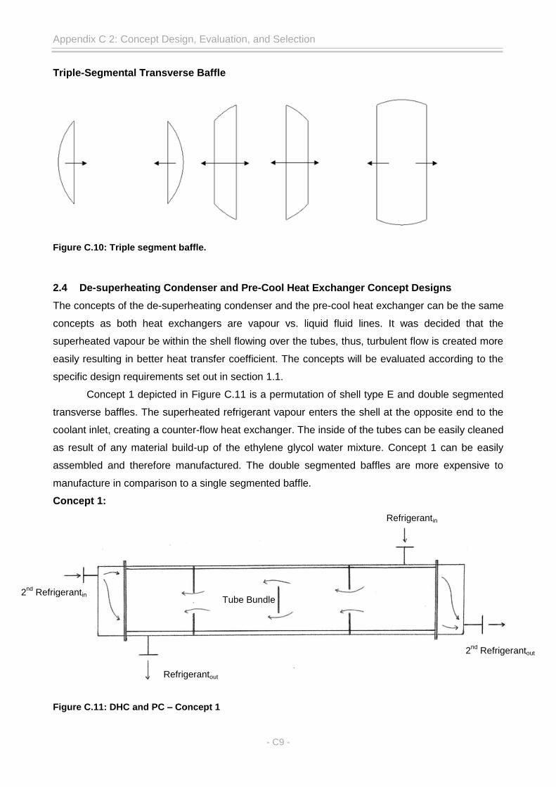
Appendix C 2: Concept Design, Evaluation, and Selection
- C9 -
Triple-Segmental Transverse Baffle
Figure C.10: Triple segment baffle.
2.4 De-superheating Condenser and Pre-Cool Heat Exchanger Concept Designs
The concepts of the de-superheating condenser and the pre-cool heat exchanger can be the same
concepts as both heat exchangers are vapour vs. liquid fluid lines. It was decided that the
superheated vapour be within the shell flowing over the tubes, thus, turbulent flow is created more
easily resulting in better heat transfer coefficient. The concepts will be evaluated according to the
specific design requirements set out in section 1.1.
Concept 1 depicted in Figure C.11 is a permutation of shell type E and double segmented
transverse baffles. The superheated refrigerant vapour enters the shell at the opposite end to the
coolant inlet, creating a counter-flow heat exchanger. The inside of the tubes can be easily cleaned
as result of any material build-up of the ethylene glycol water mixture. Concept 1 can be easily
assembled and therefore manufactured. The double segmented baffles are more expensive to
manufacture in comparison to a single segmented baffle.
Concept 1:
Figure C.11: DHC and PC – Concept 1
2nd
Refrigerantin
Refrigerantout
Tube Bundle
2nd
Refrigerantout
Refrigerantin

Appendix C 2: Concept Design, Evaluation, and Selection
- C10 -
Concept 2:
Figure C.12: DHC and PC – Concept 2
Concept 2 is depicted by Figure C.12 is a permutation of shell type E and triple segmented baffles,
creating a counter-flow heat exchanger. The refrigerant and coolant streams have the same
characteristics as concept 1, with the only difference being the lower pressure drop of concept 2.
The cost of manufacturing of concept 2 would be the highest of the 4 concept designs.
Concept 3:
Figure C.13: DHC and PC – Concept 3
Concept 3 is illustrated by Figure C.13, which is a permutation of the shell type E and single
segmented transverse baffles, creating a counter-flow heat exchanger. Concept 3 would be the
simplest to manufacture and the also the cheapest, though the pressure drop would be the highest
of the design concepts. Similar to concept 1, concept 3 would be easily cleaned at the tube side.
2nd
Refrigerantin
2nd
Refrigerantout
Refrigerantout
Tube Bundle
Refrigerantin
2nd
Refrigerantin
2nd
Refrigerantout
Refrigerantout
Tube Bundle
Refrigerantin

Appendix C 2: Concept Design, Evaluation, and Selection
- C11 -
Concept 4:
Figure C.14: DHC and PC – Concept 4
The final concept is depicted in Figure C.14, and is a permutation of shell type J and single
segmented baffles. The aqueous ammonia refrigerant flows into the shell side via two inlets and
exits via a central outlet. The flow of the shell side has both parallel and counter-flow, which might
not be optimal for the heat transfer rating and heat transfer coefficient.
Each of the subsequent concept design evaluation tables will be ranked with a weighted
importance scale and a 1 to 4 ranking of each criterion, which works as follows:
1 = Requirement not met.
2 = Requirement partially met.
3 = Requirement sufficiently met.
4 = Requirement excellently met.
Table C.4: De-superheating condenser and Pre-cool HTEX concept evaluation.
Criteria Weighted
Importance
Concepts
1 2 3 4 Thermodynamic Requirements
Heat transfer rating 1 3 3 3 3
Heat transfer coefficient 1 3 4 3 3
Stream allocation 0.7 4 4 4 4
Coolant outlet temperatures 0.8 3 3 3 3
Number of tubes 0.7 3 3 3 3
Number of tube passes 0.7 4 4 4 4
Heat transfer surface length 0.8 3 3 3 3
Pressure drop 0.4 3 4 3 2
Total 6.1 4.925 5.275 4.925 4.825
2nd
Refrigerantin
2nd
Refrigerantout
Refrigerantout
Tube Bundle
Refrigerantin Refrigerantin

Appendix C 2: Concept Design, Evaluation, and Selection
- C12 -
Table C.4 continued:
Fluid Flow Requirements
Fluid distribution 0.7 3 3 3 3
Blockage of fluids 0.7 3 3 3 2
Thermo siphoning flow 0.8 3 4 3 3
Total 2.2 1.65 1.85 1.65 1.475
Mechanical Module Requirements
Size 0.5 3 3 3 3
Mass 0.5 4 4 4 4
Safety requirements 0.9 4 4 4 4
Cost effectiveness 0.8 2 1 4 3
Maintainability 0.6 3 3 4 3
Seal 1 4 4 4 4
Separate fluids 0.9 3 3 3 3
Piping and fittings 0.8 3 3 3 3
Manufacturability 0.7 2 1 4 4
Total 6.7 5.25 4.875 6.15 5.8
Grand Total 15 11.825 12 12.725 12.1
Percentage 100 78.833 80 84.833 80.667
In conclusion, Table C.4 suggests that concept 3 would be the best alternative to which the
thermodynamic design sizing and mechanical design should represent. Though concept 3 might
have a slightly larger pressure drop to that of concept 1 and 2, it does make economically more
sense as it is cheaper to manufacture and to maintain.
2.5 Condenser Concept Designs
Concepts for the condenser module have been created using the knowledge obtained from the
standardised shell types of which are specialised to condenser units. The concepts generated are
permutations of shell type J and X, with variances of inlets, outlets and baffles. Though it is
convention for the high pressure refrigerant to be allocated to tube side, for the condenser it is
decided that the condensing aqueous-ammonia refrigerant be allocated to the shell side.
Figure C.15 illustrates the first concept of the condenser module, and it is simply a
representation of shell type J. Saturated aqua-ammonia vapour enters the shell side via two inlets
and exits the shell as saturated liquid at a central outlet, which creates a cross-flow heat
exchanger. A distribution volume added to the top of the design facilitates the distributing of aqua-
ammonia vapour over the entire length of the heat exchanger. Concept 1 has very low pressure
drops, as it is specifically used for condenser applications.

Appendix C 2: Concept Design, Evaluation, and Selection
- C13 -
Concept 1:
Figure C.15: Condenser – Concept 1
Concept 2:
Figure C.16: Condenser – Concept 2
Concept 2 as illustrated in Figure C.16 is a permutation of shell types H and J, where the shell has
two inlets, two horizontal baffles, and one central baffle. The horizontal baffles will split the flow,
distributing the fluid over the entire length of the condenser, thus creating a cross-flow heat
exchanger. The pressure drop of concept 2 might be higher than concept 1, and the horizontal
baffles might accumulate saturated liquid droplets.
Coolantin
Coolantout
Aqua-ammoniaout
Tube Bundle
Aqua-ammoniain
Coolantin
Aqua-ammoniaout
Coolantout
Aqua-ammoniain
Tube Bundle

Appendix C 2: Concept Design, Evaluation, and Selection
- C14 -
Concept 3:
Figure C.17: Condenser – Concept 3
Figure C.17 illustrates concept 3, which is a permutation similar to concept 2, with the only
difference being the placement and size of the horizontal baffle. Concept 3’s horizontal baffles are
closer to the inlets above the tube bundle, thus, changing the horizontal baffles to impingement
plates. The impingement plates facilitate the distribution of the vapour entering the condenser
concept. Concept 3 will have the largest pressure drop of the 4 concepts, but a similar heat
transfer coefficient to concept 2.
Concept 4:
Figure C.18: Condenser – Concept 4
Concept 4 depicted by Figure C.18 is simply a representation of shell type X, where it is specifically
used for most practical condensing applications. The saturated aqua-ammonia vapour enters the
shell via a single central inlet and exits as saturated liquid via a concentric outlet. Concept 4 has
similar pressure drop values and distribution volume to that of concept 1. Concept 4 would be the
Coolantin Tube Bundle
Aqua-ammoniain
Coolantout
Aqua-ammoniaout
Coolantin
Aqua-ammoniain
Coolantout
Aqua-ammoniaout
Tube Bundle

Appendix C 2: Concept Design, Evaluation, and Selection
- C15 -
cheapest to manufacture of the four concepts, but might be ranked lower on its shell side heat
transfer coefficient. The concept designs generated for the condenser unit are evaluated in the
following table as:
Table C.5: Condenser concept evaluation.
Criteria Weighted
Importance
Concepts
1 2 3 4 Thermodynamic Requirements
Heat transfer rating 1 3 3 3 3
Heat transfer coefficient 0.9 3 3 4 3
Q ≤ 0.00 1 3 3 3 3
Stream allocation 1 3 3 3 3
Coolant outlet temperatures 0.8 3 3 4 3
Number of tubes 0.7 3 3 3 3
Number of tube passes 0.7 4 4 4 4
Heat transfer surface length 0.8 3 3 4 3
Pressure drop 0.4 4 3 1 4
Total 7.3 5.75 5.65 6.075 5.75
Fluid Flow Requirements
Fluid distribution 0.7 4 3 4 2
Blockage of fluids 0.7 4 2 2 4
Thermo siphoning flow 0.8 4 3 3 4
Total 2.2 2.2 1.475 1.65 1.85
Mechanical Module Requirements
Size 0.5 3 4 4 3
Mass 0.5 3 3 3 3
Safety requirements 0.9 4 4 4 4
Cost effectiveness 0.8 4 2 2 4
Maintainability 0.6 4 3 3 4
Seal 1 4 4 4 4
Separate fluids 0.9 4 4 4 4
Piping and fittings 0.8 3 3 3 4
Manufacturability 0.7 4 3 3 4
Total 6.7 6.25 5.65 5.65 6.45
Grand Total 16.2 14.2 12.775 13.375 14.05
Percentage 100 87.654 78.858 82.562 86.728
To conclude, Table C.5 indicated concept 1 has the reigning concept, though concept 4 is a narrow
second. Concept 2 is cost effective, has good refrigerant distribution, and low pressure drop, which
are telling factors when designing a condenser unit.

Appendix C 2: Concept Design, Evaluation, and Selection
- C16 -
2.6 Evaporator Concept Designs
The concepts of the evaporator are permutations of type K shell, with variances in inlet and outlet
placement. The concepts also take into consideration the tertiary gas of helium within the heat
exchanger module, which creates partial pressure. Though it is convention for the high pressure
refrigerant to be allocated to tube side, for the evaporator it is decided that the evaporating
aqueous-ammonia refrigerant be allocated to the shell side and the ethylene glycol water mixture
to tube side.
Concept 1:
Figure C.19: Evaporator – Concept 1
Figure C.19 illustrates the first evaporator design concept, with is an adaptation of the shell type K,
but as a single tube pass heat exchanger. The top vapour compartment will fill the much lower
density helium that creates the partial pressure of the aqua-ammonia. The sub-cooled aqua-
ammonia liquid enters the shell at the bottom right of the shell through the venturi nozzle and exits
as saturated vapour ammonia at the top left of the shell, thus creating a counter-flow heat
exchanger with no transverse baffles. The outlet of ammonia is below the helium line to prevent
helium from exiting the evaporator. The shell would be difficult to manufacture and would require a
lot of laser cut components.
Coolantin
Aqua-ammoniain
Coolantout
Ammoniaout
Tube Bundle
Helium

Appendix C 2: Concept Design, Evaluation, and Selection
- C17 -
Concept 2:
Figure C.20: Evaporator – Concept 2
Evaporator concept 2 is illustrated by Figure C.20 and is a permutation of the shell type K, but with
a bit more manufacturability of the shell housing. The sub-cooled aqua-ammonia liquid enter the
shell via two nozzles where only one is a venturi nozzle, with the saturated vapour ammonia exiting
the shell at the top left. Concept 2 is a counter-flow heat exchanger with no transverse baffles, with
single tube pass arrangement, and top kettle compartment for helium gas.
Concept 3:
Figure C.21: Evaporator – Concept 3
Concept 3 is depicted in Figure C.21 and is a permutation of concept 2 and shell type J, where
only now sub-cooled aqua-ammonia liquid enters through a single venturi nozzle at the bottom of
the shell. The saturated ammonia vapour exits the shell opposite ends of the shell, but the outlets
must remain lower than the helium gas line to prevent helium from exiting the evaporator. Concept
3 is simpler to manufacture than the previous two concepts and has a more symmetrical cross-flow
pattern of refrigerant than the previously the mentioned concepts. Though, concept 3 might have
short comings in terms of distribution of sub-cooled liquid over the entire tube length.
Coolantin
Ammoniaout Ammoniaout
Aqua-ammoniain Aqua-ammoniain
Coolantout
Ammoniaout
Helium
Ammoniaout
Aqua-ammoniain
Coolantin
Tube Bundle
Coolantout
Helium
Tube Bundle

Appendix C 2: Concept Design, Evaluation, and Selection
- C18 -
Concept 4:
Figure C.22: Evaporator – Concept 4
Concept 3 is depicted in Figure C.22 and is an improved distribution concept of concept 3 and shell
type J, where now the sub-cooled aqua-ammonia liquid enters the evaporator from the top of the
shell via three inlets. The central inlet is the venturi nozzle, with adjacent normal nozzles to the left
and right. The saturated ammonia vapour still exits at opposite ends of the shell, but the outlets
must remain lower than the helium gas line to prevent helium from exiting the evaporator. Concept
4 has a symmetrical cross-flow to co-counter-flow pattern of refrigerant. Though, concept 4 has the
best distribution of sub-cooled liquid over the entire tube length.
The evaporator’s concept evaluation is illustrated in the following table as:
Table C.6: Evaporator concept evaluation.
Criteria Weighted
Importance
Concepts
1 2 3 4 Thermodynamic Requirements
Heat transfer rating 1 3 3 3 3
Heat transfer coefficient 0.9 3 3 3 4
Q ≤ 1.00 1 3 3 3 3
Stream allocation 1 3 3 3 3
Coolant outlet temperatures 0.8 3 3 4 4
Number of tubes 0.7 2 2 3 3
Number of tube passes 0.7 4 4 4 4
Heat transfer surface length 0.8 2 3 2 4
Partial pressure across evaporator 0.7 1 2 1 3
Total 7.6 5.15 5.525 5.525 6.5
Aqua-ammoniain
Ammoniaout Ammoniaout
Venturi
Coolantin Coolantout
Helium
Tube Bundle
Orifice

Appendix C 2: Concept Design, Evaluation, and Selection
- C19 -
Table C.6 continued:
Fluid Flow Requirements
Fluid distribution 0.7 1 3 2 3
Blockage of fluids 0.7 4 3 3 3
Thermo siphoning flow 0.8 4 2 3 3
Total 2.2 1.675 1.45 1.475 1.65
Mechanical Module Requirements
Size 0.5 2 2 2 3
Mass 0.5 2 2 2 3
Safety requirements 0.9 4 4 4 4
Cost effectiveness 0.8 4 3 3 3
Maintainability 0.6 3 3 3 3
Seal 1 4 4 4 4
Separate refrigerant and coolant 0.9 4 4 4 4
Piping and fittings 0.8 4 3 4 3
Manufacturability 0.7 2 2 2 2
Total 6.7 5.7 5.3 5.5 5.55
Grand Total 16.5 12.525 12.275 12.5 13.7
Percentage 100 75.909 74.394 75.758 83.03
To conclude the evaporator concept designs, Table C.6 shows that concept 4 has the best concept
out of the four concepts made. Concept 4 has the best distribution of sub-cooled aqua-ammonia
liquid, which will benefit the creation of partial pressure. Concept 4 has symmetric outlets to benefit
cross-flow fluid patterns and it situated at the top half of the shell assisting the low density
expanding saturated vapour ammonia.
2.7 Regenerative Heat Exchanger Concept Designs
The regenerative heat exchanger design concepts are permutations of type E, G, J, and X shell
types. The allocations of fluid streams remain open for the concept designs. Concept 1 is
illustrated in Figure C.23 and is a simple shell type E with single segmented transverse baffles.
The heat exchanger concept has counter-flow and the strong solution aqueous ammonia is
allocated to tube side heat transfer. The outlet of the strong solution is placed at the top of the
header as there is a possibility of vapour bubbles forming, which flows upwards due to its low
density. Concept 1 has simplicity and is easy to manufacture, which is therefore cheap, but does
compromise on shell side pressure drop and possible vapour entrapment.

Appendix C 2: Concept Design, Evaluation, and Selection
- C20 -
Concept 1:
Figure C.23: Regenerative heat exchanger – Concept 1
Concept 2:
Figure C.24: Regenerative heat exchanger – Concept 2
The second concept is depicted by Figure C.24 and is a permutation of shell types J and H, where
the shell has divided inlets, two horizontal baffles, but only one central outlet. The allocation of fluid
streams for concept 2 is switch around from concept 1, where the strong solution aqua-ammonia
now flows over the tubes at the shell side. Concept 2 has a cross-flow pattern upwards with
horizontal baffle splitting the flow into four fluid streams. This would benefit the heat transfer
coefficient of the shell side at the compromise of pressure loss.
ssin
wsin
Tube Bundle
ssout
wsout
ssin
ssout
wsin
wsout Tube Bundle

Appendix C 2: Concept Design, Evaluation, and Selection
- C21 -
Concept 3:
Figure C.25: Regenerative heat exchanger – Concept 3
Concept 3 is depicted by Figure C.25 and is a simple representation of shell type G, where the
shell has a single inlet and outlet, concentrically placed in the middle of the shell creating a cross-
flow pattern. The shell side has a horizontal baffle at approximately 75% of the tube length, which
splits the flow of the strong solution aqua-ammonia. Similar to concept 2 the horizontal baffle would
benefit the heat transfer coefficient of shell side, but this is at the cost of pressure loss. Concept 3
would be cheaper to manufacture than concept 1 and 2 as it has less parts to laser cut and weld.
Concept 4:
Figure C.26: Regenerative heat exchanger – Concept 4
Lastly, concept 4 is represented by Figure C.26 which is an adaptation of shell type X, with the
strong solution aqua-ammonia allocated to shell side heat transfer. Concept 4 will produce the
lowest pressure loss of the 4 concept designs, and would be the cheapest to manufacture as there
are no baffles to be laser cut. Concept 4 will have a lower heat transfer coefficient to that of
concept 2 and 3, which would result in a slightly longer heat transfer surface area.
ssin
ssout
wsin
wsout
Tube Bundle
Tube Bundle
ssin
ssout
wsin
wsout

Appendix C 2: Concept Design, Evaluation, and Selection
- C22 -
The concept designs of the regenerative heat exchanger are evaluated in the following table as:
Table C.7: Regenerative heat exchanger concept evaluation.
Criteria Weighted
Importance
Concepts
1 2 3 4 Thermodynamic Requirements
Heat transfer rating 1 3 3 3 3
Heat transfer coefficient 0.9 3 4 4 3
Stream allocation 1 4 3 3 3
Outlet temperatures 0.8 4 4 4 3
Number of tubes 0.7 3 3 3 3
Number of tube passes 0.7 4 4 4 4
Heat transfer surface length 0.8 4 3 3 3
Pressure drop 0.7 1 2 2 4
Total 6.6 5.425 5.375 5.375 5.525
Fluid Flow Requirements
Fluid distribution 0.7 3 4 4 3
Blockage of fluids 0.7 2 3 3 4
Thermo siphoning flow 0.8 2 3 3 4
Total 2.2 1.275 1.825 1.825 2.025
Mechanical Module Requirements
Size 0.5 3 3 3 2
Mass 0.5 3 3 3 3
Safety requirements 0.9 4 4 4 4
Cost effectiveness 0.8 2 3 3 4
Maintainability 0.6 3 3 3 3
Seal 1 4 4 4 4
Separate refrigerant and coolant 0.9 4 4 4 4
Piping and fittings 0.8 3 3 3 3
Manufacturability 0.7 4 4 4 4
Total 6.7 5.7 5.9 5.9 5.975
Grand Total 15.5 12.4 13.1 13.1 13.525
Percentage 100 80 84.516 84.516 85.806
In conclusion, Table C.7 indicates concept 4 as the reigning concept between the four
concepts. Concept 4 is the cheapest to manufacture, but does compromise on heat transfer
coefficient slightly. The lower heat transfer coefficient of concept 4 would translate in slightly longer
tubes lengths, but won’t cost as much as the horizontal baffles of concepts 1 and 2. Concept 4 has
the lowest pressure drop, which benefits the slight boiling of strong solution allocated to shell side
heat transfer.

Appendix C 2: Concept Design, Evaluation, and Selection
- C23 -
2.8 Auxiliary Heat Exchanger Concept Designs
The auxiliary heat exchanger design concepts are representations of shell type E, with the only
variance in the allocation of fluid lines. The concept designs are simple and effective, as the heat
exchanger consists of liquid vs. liquid heat transfer.
Concept 1:
Figure C.27: Auxiliary heat exchanger – Concept 1
Concept 1 is represented by Figure C.27, with the weak aqua-ammonia solution allocated to tube
side heat transfer. It is conventional to allocate the high pressure fluid to flow through the tubes.
Concept 2:
Figure C.28: Auxiliary heat exchanger – Concept 2
Concept 2 is depicted by Figure C.28, with the weak solution aqua-ammonia allocated to shell side
heat transfer. This allocation is chosen as it would be easier to clean the tube side ethylene glycol
water material build-up and the weak solution aqua-ammonia would have the lower heat transfer
coefficient, therefore allocating it to flow over the tubes.
Tube Bundle
Coolantout
wsin
wsout
Coolantin
wsout wsin
Coolantout
Coolantin
Tube Bundle

Appendix C 2: Concept Design, Evaluation, and Selection
- C24 -
The concept designs generated for the auxiliary heat exchanger are evaluated in the following
table as:
Table C.8: Auxiliary heat exchanger concept evaluation.
Criteria Weighted
Importance
Concepts
1 2 Thermodynamic Requirements
Heat transfer rating 1 3 3
Heat transfer coefficient 0.9 4 3
Stream allocation 1 3 4
Outlet temperatures 0.8 4 4
Number of tubes 0.7 3 3
Number of tube passes 0.7 4 4
Heat transfer surface length 0.8 4 2
Pressure drop 0.7 1 4
Total 6.6 5.4 5.55
Fluid Flow Requirements
Fluid distribution 0.7 3 3
Blockage of fluids 0.7 3 3
Thermo siphoning flow 0.8 1 4
Total 2.2 1.25 1.85
Mechanical Module Requirements
Size 0.5 3 3
Mass 0.5 3 3
Safety requirements 0.9 4 4
Cost effectiveness 0.8 3 3
Maintainability 0.6 4 2
Seal 1 4 4
Separate refrigerant and coolant 0.9 4 4
Piping and fittings 0.8 3 3
Manufacturability 0.7 4 4
Total 6.7 6.05 5.75
Grand Total 15.5 12.7 13.15
Percentage 100 81.935 84.839
In conclusion of the auxiliary heat exchanger concept designs, Table C.8 illustrates the allocation
of weak solution to tube side heat transfer be more beneficial than shell side heat transfer. Though,
concept 2 might be more difficult to maintain, the benefit of low pressure drops within the tubes far
out weight maintenance.

Appendix C 2: Concept Design, Evaluation, and Selection
- C25 -
2.9 Auxiliary-Regenerative Heat Exchanger Concept Design
The decision to use concept 4 of the regenerative heat exchanger and concept 2 of the auxiliary
heat exchangers gave the opportunity to be innovative by synthesizing the two concepts to form a
single heat exchanger module. This is made possible by the weak solution aqua-ammonia flowing
through the tubes for both concepts. The newly formed synthesized Aux-Regen HTEX is illustrated
by Figure C.29 below.
Figure C.29: Auxiliary-Regenerative heat exchanger concept design.
ssout
wsout
wsin
Coolantout Coolantin
Tube Bundle Auxiliary
Regen
ssin

Appendix D 1
Extended Chapter 4 - Thermodynamic Design
Summary
Recorded in Appendix D 1 is an extension of the omitted temperature vs. unit surface area figures and an
explanatory guide of further Appendix D documentation. The explanatory guide focuses on the layout of the
rest of the appendix, in terms of folder to file references to guide the reader to each heat exchanger’s MS
Excel thermodynamic design model and the EES verification thereof.

- i -
Table of Contents
1 TEMPERATURE VS. UNIT SURFACE AREA ................................................................ D 1.1
1.1 Stage 1 Condenser .................................................................................................... D 1.3
1.2 Stage 2 Condenser .................................................................................................... D 1.4
1.3 De-superheating Condenser ...................................................................................... D 1.5
1.4 Pre-Cool Heat Exchanger .......................................................................................... D 1.6
1.5 Evaporator ................................................................................................................. D 1.7
1.6 Regenerative Heat Exchanger ................................................................................... D 1.8
1.7 Auxiliary Heat Exchanger .......................................................................................... D 1.9
1.8 Appendix D Explanatory Guide ................................................................................ D 1.10
1.8.1 Stage 1 Condenser – Thermodynamic Design Model ...................................... D 1.10
1.8.2 Stage 2 Condenser – Thermodynamic Design Model ...................................... D 1.11
1.8.3 De-superheating Condenser – Thermodynamic Design Model ........................ D 1.11
1.8.4 Pre-Cool Heat Exchanger – Thermodynamic Design Model ............................ D 1.12
1.8.5 Venturi Nozzle and Orifice ............................................................................... D 1.12
1.8.6 Evaporator – Thermodynamic Design Model ................................................... D 1.13
1.8.7 Auxiliary-Regenerative Heat Exchanger – Thermodynamic Design Model ....... D 1.13
List of Tables
Table D 1.1: Stage 1 condenser - Inlet and outlet temp for summer ambient conditions. .......... D 1.1
Table D 1.2: Stage 2 condenser - Inlet and outlet temp for winter ambient conditions. .............. D 1.1
Table D 1.3: De-superheating cond - Inlet and outlet temp for summer ambient conditions. ..... D 1.1
Table D 1.4: Pre-Cool HTEX - Inlet and outlet temp for summer ambient conditions. ................ D 1.1
Table D 1.5: Evaporator - Inlet and outlet temp for summer ambient conditions. ....................... D 1.1
Table D 1.6: Regenerative HTEX - Inlet and outlet temp for winter ambient conditions. ............ D 1.2
Table D 1.7: Auxiliary HTEX - Inlet and outlet temp for winter ambient conditions. .................... D 1.2

- ii -
List of Figures
Figure D 1.1: Stage 1 Condenser – Temperature vs. unit surface area. .................................... D 1.3
Figure D 1.2: Stage 2 Condenser – Temperature vs. unit surface area. .................................... D 1.4
Figure D 1.3: De-superheating Condenser – Temperature vs. unit surface area. ...................... D 1.5
Figure D 1.4: Pre-Cool Heat Exchanger – Temperature vs. unit surface area. .......................... D 1.6
Figure D 1.5: Evaporator – Temperature vs. unit surface area. ................................................. D 1.7
Figure D 1.6: Regenerative Heat Exchanger – Temperature vs. unit surface area. ................... D 1.8
Figure D 1.7: Auxiliary Heat Exchanger – Temperature vs. unit surface area. ........................... D 1.9
Figure D 1.8: Stage 1 Condenser – Thermodynamic design model directory. ......................... D 1.10
Figure D 1.9: Stage 2 Condenser – Thermodynamic design model directory. ......................... D 1.11
Figure D 1.10: De-superheating Condenser – Thermodynamic design model directory. ......... D 1.11
Figure D 1.11: Pre-Cool Heat Exchanger – Thermodynamic design model directory. ............. D 1.12
Figure D 1.12: Venturi Nozzle and Orifice – Design, experimental setup, and results. ............ D 1.12
Figure D 1.13: Evaporator – Thermodynamic design sizing directory. ..................................... D 1.13
Figure D 1.14: Aux-Regen Heat Exchanger – Thermodynamic design model directory. ......... D 1.13

- D 1.1 -
1 TEMPERATURE VS. UNIT SURFACE AREA
Presented in the tables below are the inlet and outlet temperatures of each heat exchanger for
their respective design conditions.
Table D 1.1: Stage 1 condenser - Inlet and outlet temp for summer ambient conditions.
Parameter Inlet Temp [°C] Outlet Temp [°C]
Refrigerant 28 (State TP) 23 (State 5)
Coolant 18.404 22.653
Table D 1.2: Stage 2 condenser - Inlet and outlet temp for winter ambient conditions.
Parameter Inlet Temp [°C] Outlet Temp [°C]
Refrigerant 47.681 (State 4) 28 (State TP)
Coolant 4.133 46
Table D 1.3: De-superheating cond - Inlet and outlet temp for summer ambient conditions.
Parameter Inlet Temp [°C] Outlet Temp [°C]
Refrigerant 95.36 (State 3) 60.055 (State 4)
Coolant 56.5 82.712
Table D 1.4: Pre-Cool HTEX - Inlet and outlet temp for summer ambient conditions.
Parameter Inlet Temp [°C] Outlet Temp [°C]
‘Hot’ Refrigerant 23 (State 5) 8.353 (State 6)
‘Cold’ Refrigerant -15 (State 9) 15.11 (State 10)
Table D 1.5: Evaporator - Inlet and outlet temp for summer ambient conditions.
Parameter Inlet Temp [°C] Outlet Temp [°C]
Refrigerant -15 (State 8) -15 (State 9)
Coolant 10 -14.5

Appendix D 1: Extended Thermodynamic Design – Temperature vs. Unit Surface Area
- D 1.2 -
Table D 1.6: Regenerative HTEX - Inlet and outlet temp for winter ambient conditions.
Parameter Inlet Temp [°C] Outlet Temp [°C]
Strong solution 33.223 49.55
Weak solution 61.72 44.94
Table D 1.7: Auxiliary HTEX - Inlet and outlet temp for winter ambient conditions.
Parameter Inlet Temp [°C] Outlet Temp [°C]
Weak Solution 44.94 5
Coolant 0.455 43
The following figures represent the temperature vs. unit surface area of each heat exchanger, where these
graphical representations are approximated as linear but are logarithmic in nature. The linear
approximation is made possible by the design assumption that the overall heat transfer coefficient is
constant and uniform across the length of the heat exchanger surface area.

Appendix D 1: Extended Thermodynamic Design – Temperature vs. Unit Surface Area
- D 1.3 -
1.1 Stage 1 Condenser
Figure D 1.1: Stage 1 Condenser – Temperature vs. unit surface area.
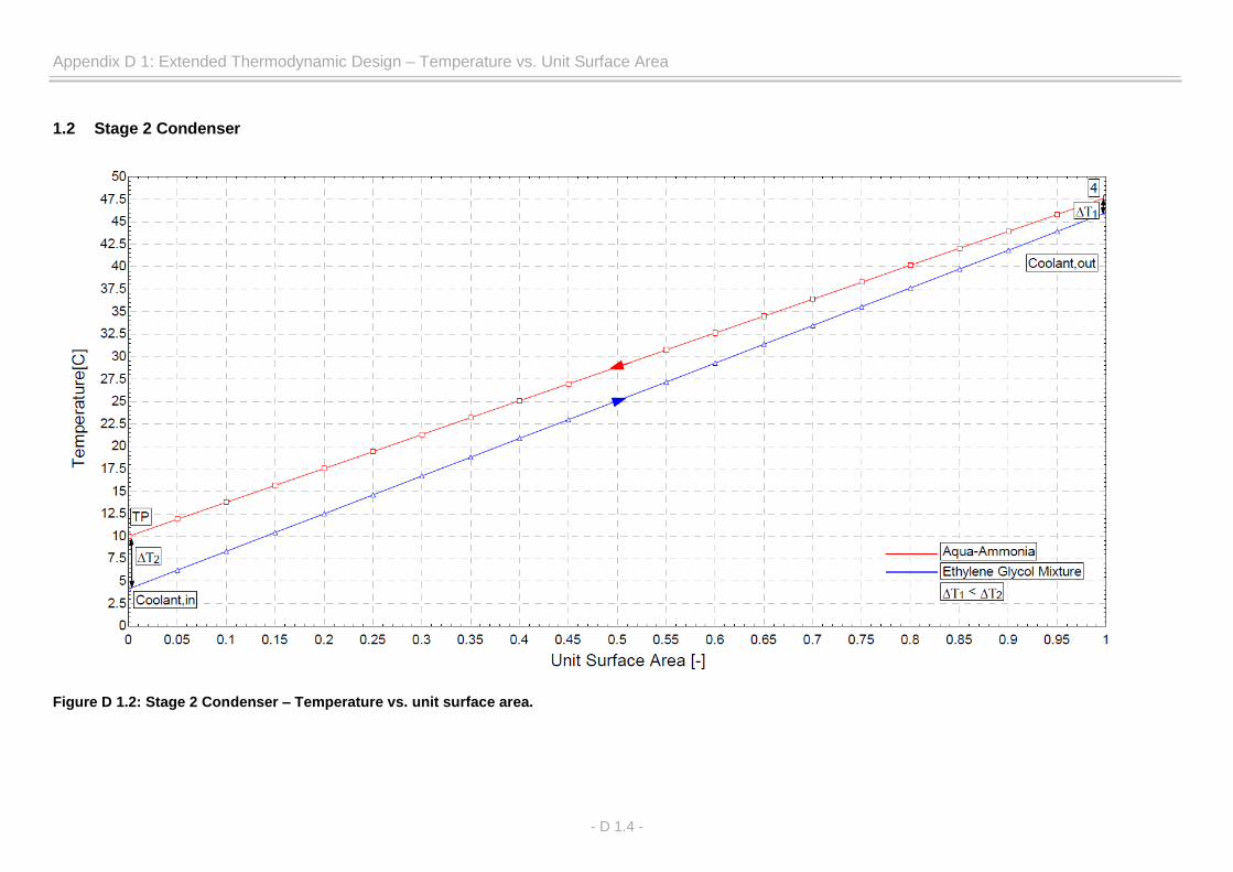
Appendix D 1: Extended Thermodynamic Design – Temperature vs. Unit Surface Area
- D 1.4 -
1.2 Stage 2 Condenser
Figure D 1.2: Stage 2 Condenser – Temperature vs. unit surface area.

Appendix D 1: Extended Thermodynamic Design – Temperature vs. Unit Surface Area
- D 1.5 -
1.3 De-superheating Condenser
Figure D 1.3: De-superheating Condenser – Temperature vs. unit surface area.

Appendix D 1: Extended Thermodynamic Design – Temperature vs. Unit Surface Area
- D 1.6 -
1.4 Pre-Cool Heat Exchanger
Figure D 1.4: Pre-Cool Heat Exchanger – Temperature vs. unit surface area.

Appendix D 1: Extended Thermodynamic Design – Temperature vs. Unit Surface Area
- D 1.7 -
1.5 Evaporator
Figure D 1.5: Evaporator – Temperature vs. unit surface area.

Appendix D 1: Extended Thermodynamic Design – Temperature vs. Unit Surface Area
- D 1.8 -
1.6 Regenerative Heat Exchanger
Figure D 1.6: Regenerative Heat Exchanger – Temperature vs. unit surface area.

Appendix D 1: Extended Thermodynamic Design – Temperature vs. Unit Surface Area
- D 1.9 -
1.7 Auxiliary Heat Exchanger
Figure D 1.7: Auxiliary Heat Exchanger – Temperature vs. unit surface area.

Appendix D 1.8: Explanatory Guide to Appendix D
- D 1.10 -
1.8 Appendix D Explanatory Guide
The following section focuses on the layout of the rest of the appendix, in terms of folder to file
references to guide the reader to each heat exchanger’s thermodynamic design sizing model and
the verification thereof. For example Appendix D 2 contains two files of the stage 1 condenser,
namely, the Excel Sizing model and the EES verification in pdf format.
1.8.1 Stage 1 Condenser – Thermodynamic Design Model
Stage 1 condenser has its folder to files directory illustrated by Figure D 1.8, where locked Excel
Workbook illustrates the model used to determine the stage 1 condenser heat transfer surface
area, and an EES model to depict the verification of the design sizing model in pdf format.
Figure D 1.8: Stage 1 Condenser – Thermodynamic design model directory.

Appendix D 1.8: Explanatory Guide to Appendix D
- D 1.11 -
1.8.2 Stage 2 Condenser – Thermodynamic Design Model
Stage 2 condenser has its folder to files directory illustrated by Figure D 1.9, where locked Excel
Workbook illustrates the model used to determine the stage 2 condenser heat transfer surface
area, and an EES model to depict the verification of the design sizing model in pdf format.
Figure D 1.9: Stage 2 Condenser – Thermodynamic design model directory.
1.8.3 De-superheating Condenser – Thermodynamic Design Model
The de-superheating condenser has its folder to files directory illustrated by Figure D 1.10, where
locked Excel Workbook illustrates the model used to determine the de-superheating condenser
heat transfer surface area, and an EES model to depict the verification of the design sizing model
in pdf format.
Figure D 1.10: De-superheating Condenser – Thermodynamic design model directory.
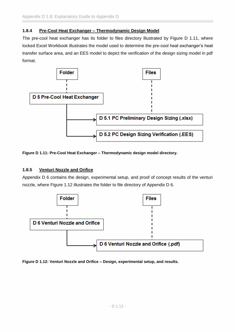
Appendix D 1.8: Explanatory Guide to Appendix D
- D 1.12 -
1.8.4 Pre-Cool Heat Exchanger – Thermodynamic Design Model
The pre-cool heat exchanger has its folder to files directory illustrated by Figure D 1.11, where
locked Excel Workbook illustrates the model used to determine the pre-cool heat exchanger’s heat
transfer surface area, and an EES model to depict the verification of the design sizing model in pdf
format.
Figure D 1.11: Pre-Cool Heat Exchanger – Thermodynamic design model directory.
1.8.5 Venturi Nozzle and Orifice
Appendix D 6 contains the design, experimental setup, and proof of concept results of the venturi
nozzle, where Figure 1.12 illustrates the folder to file directory of Appendix D 6.
Figure D 1.12: Venturi Nozzle and Orifice – Design, experimental setup, and results.

Appendix D 1.8: Explanatory Guide to Appendix D
- D 1.13 -
1.8.6 Evaporator – Thermodynamic Design Model
The evaporator has its folder to files directory illustrated by Figure D 1.13, where locked Excel
Workbook illustrates the model used to determine the evaporator’s heat transfer surface area, and
an EES model to depict the verification of the design sizing model in pdf format.
Figure D 1.13: Evaporator – Thermodynamic design sizing directory.
1.8.7 Auxiliary-Regenerative Heat Exchanger – Thermodynamic Design Model
The auxiliary-regenerative heat exchanger has its folder to files directory illustrated by Figure D
1.14, where locked Excel Workbook illustrates the model used to determine the aux-regen’s heat
transfer surface area, and an EES model to depict the verification of the design sizing model in pdf
format.
Figure D 1.14: Aux-Regen Heat Exchanger – Thermodynamic design model directory.

Appendix D 6
Extended Chapter 4 – Venturi Nozzle Design, Experimental Setup
and Results
Summary
Appendix D 6 aims to explain the design and experimental setup behind the venturi nozzle, which
is required for the thermodynamic design of the evaporator module. The venturi nozzle is designed
using Bernoulli’s equations set in Chapter 4. Compiled within this appendix are the manufacturing
drawings of the venturi nozzle, the experimental setup and results. The experimental setup tries to
emulate the conditions under which the venturi nozzle will operate within the aqua-ammonia
absorption-desorption cycle, where the operating conditions are converted into a gravitational
water flow system with the equivalent head pressure. The experiments are used as a proof of
concept, not as a full venturi flow analysis.

- i -
Table of Contents
6 VENTURI NOZZLE EXPERIMENTAL SETUP AND RESULTS .................................... D 6.1
6.1 Experimental Setup Calculations ............................................................................... D 6.1
6.2 Experimental Results ................................................................................................. D 6.3
List of Tables
Table D 6.1: Density properties for experimental representation of the liquid column in the aqua-
ammonia absorption-desorption cycle. .................................................................... D 6.1
Table D 6.2: Standard discharge coefficients (Engineeringtoolbox, 2015). ................................ D 6.5
List of Figures
Figure D 6.1: Component schematic of the liquid column flowing towards the venturi nozzle. ... D 6.1
Figure D 6.2: Venturi proof of concept experimental setup. ....................................................... D 6.2
Figure D 6.3: Venturi nozzle – Manufacturing and assembly design. ........................................ D 6.3
Figure D 6.4: Venturi nozzle suction height results. ................................................................... D 6.4

- D 6.1 -
6 VENTURI NOZZLE EXPERIMENTAL SETUP AND RESULTS
6.1 Experimental Setup Calculations
The venturi nozzle is designed for winter ambient conditions, due to winter conditions having the
lowest mass flow rate of the aqua-ammonia refrigerant. Therefore, the density properties of the
fluid line entering the venturi nozzle are illustrated in Table D 6.1.
Table D 6.1: Density properties for experimental representation of the liquid column in the aqua-ammonia absorption-desorption cycle.
Density Properties
ρ3 3.351 kg/m3
ρ4 5.28899 kg/m3
ρ5 636.998 kg/m3
ρ6 648.048 kg/m3
ρw 1000 kg/m3
The schematic component diagram of the aqua-ammonia absorption-desorption H&R cycle is
illustrated in Figure D 6.1, where the height of each segment of the fluid column leading towards
the venturi is shown. The total height from the base of the evaporator to the top of the de-
superheating condenser is 1.8 m, and the venturi nozzle is 0.4 m from the base of the evaporator.
Thus, leaving a total of 1.4 m for the fluid line from the de-superheating condenser to the outlet of
the venturi nozzle in the evaporator.
Figure D 6.1: Component schematic of the liquid column flowing towards the venturi nozzle.

Appendix D 6: Venturi Nozzle Design, and Experimental Setup and Results
- D 6.2 -
Experimental Setup Height
As water will be used during the experiment, the experimental head needs to be determined to
equal the head of the H&R cycle. Thus, it can be assumed that the head height of the H&R cycle is
equal to the head height of the experimental setup. The experimental head height is calculated as:
Experimental Setup
The experimental setup that was used to complete the proof of venturi concept is illustrated in
Figure D 6.2, with the design of the venturi nozzle illustrated in Figure D 6.3.
Figure D 6.2: Venturi proof of concept experimental setup.
𝐻𝑐𝑦𝑐𝑙𝑒 = 𝐻𝑒𝑥𝑝𝑒𝑟𝑖𝑚𝑒𝑛𝑡
𝜌𝑔ℎ1 + 𝜌𝑔ℎ2 + 𝜌𝑔ℎ3 = 𝜌𝑔ℎ𝑒𝑥𝑝𝑒𝑟𝑖𝑚𝑒𝑛𝑡
𝜌3 + 𝜌4
2 ℎ1 +
𝜌4 + 𝜌52
ℎ2 + 𝜌6 ℎ3 = 𝜌𝑤ℎ𝑒𝑥𝑝𝑒𝑟𝑖𝑚𝑒𝑛𝑡
∴ ℎ𝑒𝑥𝑝𝑒𝑟𝑖𝑚𝑒𝑛𝑡 = 3.351+5.28899
2 0.5 +
5.2889+636.998
2 0.3 + 648.048 0.6
1000
∴ ℎ𝑒𝑥𝑝𝑒𝑟𝑖𝑚𝑒𝑛𝑡 = 0.487332 [𝑚]
∴ ≅ 0.490 [𝑚]

Appendix D 6: Venturi Nozzle Design, and Experimental Setup and Results
- D 6.3 -
Figure D 6.3: Venturi nozzle – Manufacturing and assembly design.
6.2 Experimental Results
The experimental results of the venturi nozzle are available in Figure D 6.4, with supporting video
documentation in Appendix D 6, namely, Appendix D 6.2 Experimental Results.mp4.
Helium Aqua-Ammonia

Appendix D 6: Venturi Nozzle Design, and Experimental Setup and Results
- D 6.4 -
Figure D 6.4: Venturi nozzle suction height results.
As illustrated in Figure D 6.4, the venturi nozzle created a negative pressure strong enough to lift
water to a total height of 101 mm. The starting point of the water meniscus is at 12 mm, with the
water being sucked to a height of 113 mm, indicated. Taking the height of the water suction line
and substituting it into a head calculation equation yields a suction pressure of:
∴ 𝑃 = 𝜌𝑤𝑔ℎ𝑟𝑒𝑠𝑢𝑙𝑡
∴ = 1000 9.81 0.101
∴ = 990.81 [𝑃𝑎]
∴ ≅ 1 [𝑘𝑃𝑎] 𝑆𝑢𝑐𝑡𝑖𝑜𝑛

Appendix D 6: Venturi Nozzle Design, and Experimental Setup and Results
- D 6.5 -
The fact that the venturi was able to produce a negative pressure great enough to lift water up a
tube 101 mm validates that the venturi nozzle has a feasible and functioning design to be
implemented into the evaporator module.
Venturi Nozzle Drainage and Discharge Coefficient
The venturi nozzle was designed with an assumed discharge coefficient (in Chapter 4.4) of 0.9 [-],
which is a typical value for smooth reducing nozzles, but the design of the venturi nozzle required a
step reduction in diameter due to the small orifice diameter. Thus, after the experiment it is now
possible to determine the practical value of the venturi nozzle. The venturi nozzle needed 138.4
seconds to drain 1 litre of water, with a discharge velocity of 2.30 [m/s]. The discharge velocity is
slightly lower than what was calculated in Chapter 4.4, but was expected as the discharge
coefficient was assumed to be 0.9 [-]. Now, by using the volumetric flow rate of 7.225 x 10⁻⁶ [m3/s],
and Eq. 4.4, the discharge coefficient is calculated as:
Standard discharge coefficients for various orifices are illustrated in Table D 6.2.
Table D 6.2: Standard discharge coefficients (Engineeringtoolbox, 2015).
Discharge Coefficient - CD
Diameter Ratio
d = D2/D1
Reynolds Number - Re
104 105 106 107
0.2 0.968 0.988 0.994 0.995
0.4 0.957 0.984 0.993 0.995
0.6 0.95 0.981 0.992 0.995
0.8 0.94 0.978 0.991 0.995
𝑉 = 𝐶𝐷𝐴 2𝑔ℎ
𝐶𝐷 =𝑉
𝐴 2𝑔ℎ
∴ =7.225 x 10⁻⁶
𝜋
4 0.0022 2 9.81 0.49
∴ = 0.7417

Appendix D 9
Extended Chapter 4 – Effectiveness vs. NTU
Summary
Appendix D 9 deals with the effectiveness vs. number of transfer units of each of the rated heat
exchangers. The effectiveness, NTU, and capacity ratios are used in the figures of Appendix D 9 to
determine whether a heat exchanger lies within the practically excepted heat transfer efficiency.
The effectiveness vs. NTU plots are good indicators to whether the correct coolant boundary
conditions are implemented for each heat exchanger.

- i -
Table of Contents
9 EFFECTIVENESS VS. NTU CURVES ............................................................................. D 9.1
9.1 Stage 1 Condenser .................................................................................................... D 9.3
9.2 Stage 2 Condenser .................................................................................................... D 9.4
9.3 De-superheating condenser....................................................................................... D 9.5
9.4 Pre-Cool Heat exchanger .......................................................................................... D 9.6
9.5 Evaporator ................................................................................................................. D 9.7
9.6 Regenerative Heat exchanger ................................................................................... D 9.8
9.7 Auxiliary Heat Exchanger .......................................................................................... D 9.9
List of Tables
Table D 9.1: S1C – NTU, Effectiveness, and Capacity Ratio output values. .............................. D 9.1
Table D 9.2: S2C – NTU, Effectiveness, and Capacity Ratio output values. .............................. D 9.1
Table D 9.3: DHC – NTU, Effectiveness, and Capacity Ratio output values. ............................. D 9.1
Table D 9.4: PC – NTU, Effectiveness, and Capacity Ratio output values................................. D 9.1
Table D 9.5: Evap – NTU, Effectiveness, and Capacity Ratio output values. ............................ D 9.2
Table D 9.6: Regen – NTU, Effectiveness, and Capacity Ratio output values. .......................... D 9.2
Table D 9.7: Aux – NTU, Effectiveness, and Capacity Ratio output values. .............................. D 9.2
List of Figures
Figure D 9.1: Stage 1 condenser – Effectiveness vs. NTU rating. ............................................. D 9.3
Figure D 9.2: Stage 2 condenser – Effectiveness vs. NTU rating. ............................................. D 9.4
Figure D 9.3: De-superheating condenser – Effectiveness vs. NTU rating. ............................... D 9.5
Figure D 9.4: Pre-cool heat exchanger – Effectiveness vs. NTU rating. .................................... D 9.6
Figure D 9.5: Evaporator – Effectiveness vs. NTU rating. ......................................................... D 9.7
Figure D 9.6: Regenerative heat exchanger – Effectiveness vs. NTU rating. ............................ D 9.8
Figure D 9.7: Auxiliary heat exchanger – Effectiveness vs. NTU rating. .................................... D 9.9

- D 9.1 -
9 EFFECTIVENESS VS. NTU CURVES
Illustrated in the tables below are the NTU, effectiveness, and capacity ratio of all ambient design
conditions for all the sized heat exchangers.
Table D 9.1: S1C – NTU, Effectiveness, and Capacity Ratio output values.
Parameter NTU ε c
Summer Ambient 50.0753 1 0.02252
Average Ambient 49.2701 1 0.02227
Winter Ambient 48.8386 1 0.02193
Table D 9.2: S2C – NTU, Effectiveness, and Capacity Ratio output values.
Parameter NTU ε c
Summer Ambient 6.3260 0.82987 0.82056
Average Ambient 9.8643 0.81706 0.97111
Winter Ambient 16.005 0.90497 0.78114
Table D 9.3: DHC – NTU, Effectiveness, and Capacity Ratio output values.
Parameter NTU ε c
Summer Ambient 4.8181 0.90093 0.75932
Average Ambient 3.9027 0.89167 0.65559
Winter Ambient 2.7280 0.81709 0.66395
Table D 9.4: PC – NTU, Effectiveness, and Capacity Ratio output values.
Parameter NTU ε c
Summer Ambient 1.0399 0.57752 0.49601
Average Ambient 1.1109 0.59325 0.53021
Winter Ambient 1.1207 0.59514 0.53592

Appendix D 9: Extended Thermodynamic Design and Rating – Effectiveness vs. NTU
- D 9.2 -
Table D 9.5: Evap – NTU, Effectiveness, and Capacity Ratio output values.
Parameter NTU ε c
Summer Ambient 32.1550 1 0.05976
Average Ambient 32.5935 1 0.05896
Winter Ambient 33.1197 1 0.05802
Table D 9.6: Regen – NTU, Effectiveness, and Capacity Ratio output values.
Parameter NTU ε c
Summer Ambient 0.62549 0.37879 0.82655
Average Ambient 1.20066 0.53473 0.85029
Winter Ambient 1.16130 0.59809 0.88102
Table D 9.7: Aux – NTU, Effectiveness, and Capacity Ratio output values.
Parameter NTU ε c
Summer Ambient 13.8055 0.84448 0.95678
Average Ambient 16.0829 0.84236 0.99715
Winter Ambient 11.8119 0.86741 0.84953
Effectiveness vs. NTU Curve Legend
The standard effectiveness vs. NTU curve figures are obtained from (www.gcns.ac.uk, 2005)

- D 9.3 -
9.1 Stage 1 Condenser
Figure D 9.1: Stage 1 condenser – Effectiveness vs. NTU rating.

- D 9.4 -
9.2 Stage 2 Condenser
Figure D 9.2: Stage 2 condenser – Effectiveness vs. NTU rating.

- D 9.5 -
9.3 De-superheating condenser
Figure D 9.3: De-superheating condenser – Effectiveness vs. NTU rating.

- D 9.6 -
9.4 Pre-Cool Heat exchanger
Figure D 9.4: Pre-cool heat exchanger – Effectiveness vs. NTU rating.

- D 9.7 -
9.5 Evaporator
Figure D 9.5: Evaporator – Effectiveness vs. NTU rating.

- D 9.8 -
9.6 Regenerative Heat exchanger
Figure D 9.6: Regenerative heat exchanger – Effectiveness vs. NTU rating.

- D 9.9 -
9.7 Auxiliary Heat Exchanger
Figure D 9.7: Auxiliary heat exchanger – Effectiveness vs. NTU rating.

Appendix E
Mechanical Considerations and Design
Summary
This appendix focuses on the mechanical design of the sized heat exchanger models by using the
necessary considerations that are required to complete the design of the heat exchangers for the
solar-powered aqua-ammonia absorption-desorption H&R cycle. Appendix E also consists of the
manufacturing and assembly drawings of each individual heat exchanger, together with component
‘nesting’ drawings of connecting pipes.

- i -
Table of Contents
1 MECHANICAL CONSIDERATIONS AND DESIGNS ......................................................... E1
1.1 Tube Sheet Thickness Calculations ............................................................................... E1
1.2 Shell Stress Calculations ............................................................................................... E1
1.3 Tube Stress Calculations – Design Pressure Inside ...................................................... E3
1.4 Tube Stress Calculations – Design Pressure Outside .................................................... E3
1.5 Header Bolt Calculations ............................................................................................... E4
1.6 Appendix E explanatory guide ....................................................................................... E5
1.6.1 Stage 1 Condenser Manufacturing & Assembly Drawings ..................................... E6
1.6.2 Stage 2 Condenser Manufacturing & Assembly Drawings ..................................... E7
1.6.3 De-superheating Condenser Manufacturing & Assembly Drawings ....................... E8
1.6.4 Pre-Cool Heat Exchanger Manufacturing & Assembly Drawings............................ E9
1.6.5 Evaporator Manufacturing & Assembly Drawings ................................................ E10
1.6.6 Auxiliary-Regenerative Heat Exchanger Manufacturing & Assembly Drawings .... E11
1.6.7 Aqua-Ammonia H&R Unit Manufacturing & Assembly Drawings .......................... E12
1.7 Manufacturing and assembly process .......................................................................... E13
List of Tables
Table E.1: Tube sheet thickness of Ds = 0.1345 [m]. ..................................................................... E1
Table E.2: Tube sheet thickness of Ds = 0.26467 [m]. ................................................................... E1
Table E.3: Tube sheet thickness of Ds = 0.34768 [m]. ................................................................... E1
Table E.4: Output values of shell stress calculations of Ds = 0.1345 [m]. ...................................... E2
Table E.5: Output values of shell stress calculations of Ds = 0.26467 [m]. .................................... E2
Table E.6: Output values of shell stress calculations of Ds = 0.34768 [m]. .................................... E2
Table E.7: Output values of tube stress calculations (19.1 mm) – Pressure inside. ....................... E3
Table E.8: Output values of tube stress calculations (31.8 mm) – Pressure inside. ....................... E3
Table E.9: Output values of tube stress calculations (19.1 mm) – Pressure outside. ..................... E4
Table E.10: Output values of tube stress calculations (31.8 mm) – Pressure outside. ................... E4
Table E.11: Total design force working in on the bolts. ................................................................. E4
Table E.12: Number of bolts required per heat exchanger. ........................................................... E5

- ii -
List of Figures
Figure E.1: Stage 1 Condenser – Drawings directory. ................................................................... E6
Figure E.2: Stage 2 condenser – Drawings directory. ................................................................... E7
Figure E.3: De-superheating condenser – Drawings directory....................................................... E8
Figure E.4: Pre-Cool heat exchanger – Drawings directory. .......................................................... E9
Figure E.5: Evaporator – Drawings directory. .............................................................................. E10
Figure E.6: Auxiliary-Regenerative heat exchanger – Drawings directory. .................................. E11
Figure E.7: Aqua-Ammonia H&R Unit Drawings Directory .......................................................... E12
Figure E.8: Laser Cut Components ............................................................................................. E13
Figure E.9: Tube Bundle Assembly Process ............................................................................... E14
Figure E.10: Tube Bundle Cleaning Process ............................................................................... E15
Figure E.11: Completed Aqua-Ammonia Heat Exchangers ......................................................... E15

- E1 -
1 MECHANICAL CONSIDERATIONS AND DESIGNS
1.1 Tube Sheet Thickness Calculations
The thickness of the tube sheet will be the same for the heat exchangers with the same design
pressure and tube sheet diameters. According to the ASME Code the allowable stress for stainless
steel 304L tube sheet is 205 [MPa]. Illustrated in Tables E.1, 2, and 3 are the thickness
calculations for the 0.1345 [m], 0.26467 [m], and 0.34768 [m] tube sheet, respectively. The
thicknesses are calculated using both first order and TEMA standards calculations.
Table E.1: Tube sheet thickness of Ds = 0.1345 [m].
Ds [m] PD [kPa] σallow [MPa] η t [mm] Correlation
First Order 0.1345 1400 205 - 4.8129 Eq. A.28
TEMA 0.1345 1400 205 0.5 5.2397 Eq. A.29
Table E.2: Tube sheet thickness of Ds = 0.26467 [m].
Ds [m] PD [kPa] σallow [MPa] η t [mm] Correlation
First Order 0.26467 1400 205 - 9.4709 Eq. A.28
TEMA 0.26467 1400 205 0.5 10.311 Eq. A.29
Table E.3: Tube sheet thickness of Ds = 0.34768 [m].
Ds [m] PD [kPa] σallow [MPa] η t [mm] Correlation
First Order 0.34768 1400 205 - 12.441 Eq. A.28
TEMA 0.34768 1400 205 0.5 13.544 Eq. A.29
1.2 Shell Stress Calculations
The shell stress calculations consists of axial, hoop, and radial stress calculations, which are used
to determine the safety factor of the shell housing. Recorded in the Tables E.4, 5, and 6 are the
results of the abovementioned stresses acting on the three shell sizes, with their respective
minimum shell thicknesses. Secondly, an ASME standards calculation of Appendix A 3.2, is used
to prove that the wall thickness of the shell is sufficient.
Standard stainless steel 304L nominal bore welded pipe is used for the shells of the heat
exchangers, with:
Ds = 0.1345 [m]; t = 3.4 [mm];
Ds = 0.26467 [m]; t = 4.19 [mm];
Ds = 0.34768 [m]; t = 3.96 [mm].

Appendix E 1: Mechanical Considerations and Designs
- E2 -
The internal design pressure is equal to 1.4 [MPa] and the external pressure is equal to
atmospheric pressure.
Where:
PD = 1.4 [MPa];
Do = the outer diameter of the shell;
S = 115 [MPa];
E = 0.85;
W = 1.0;
Y = 0.4,
for the calculation of the AMSE minimum thickness.
Table E.4: Output values of shell stress calculations of Ds = 0.1345 [m].
Parameter Output [Units] Correlation
Axial stress: σa 12.5153 [MPa] Eq. A.29
Hoop stress: σc 25.7618 [MPa] Eq. A.30
Radial stress: σr -0.73114 [MPa] Eq. A.31
Safety factor: SF 4.67 [-] Eq. A.33
Minimum diameter: tm 0.9577 [mm] Eq. A.32
Table E.5: Output values of shell stress calculations of Ds = 0.26467 [m].
Parameter Output [Units] Correlation
Axial stress: σa 20.2322 [MPa] Eq. A.29
Hoop stress: σc 41.2044 [MPa] Eq. A.30
Radial stress: σr -0.7400 [MPa] Eq. A.31
Safety factor: SF 2.8 [-] Eq. A.33
Minimum diameter: tm 1.81 [mm] Eq. A.32
Table E.6: Output values of shell stress calculations of Ds = 0.34768 [m].
Parameter Output [Units] Correlation
Axial stress: σa 28.2850 [MPa] Eq. A.29
Hoop stress: σc 57.3142 [MPa] Eq. A.30
Radial stress: σr -0.74427 [MPa] Eq. A.31
Safety factor: SF 2.01 [-] Eq. A.33
Minimum diameter: tm 2.48 [mm] Eq. A.32

Appendix E 1: Mechanical Considerations and Designs
- E3 -
Therefore, it can be concluded that the design decision to use welded nominal bore pipe as
the shell housing all of the heat exchanger designs is feasible and will have a safety factor in
excess of 2 [-].
1.3 Tube Stress Calculations – Design Pressure Inside
With the design pressure being on the inside of the tubes, there is a risk of the tubes
bursting. Therefore, it’s vital to calculate whether the tubes wall thickness is sufficient to
contain the high pressure aqua-ammonia refrigerant. To determine the maximum stress
within the tube walls a thin walled analysis is required. The results of the analysis are
tabulated in Table E.7 for the 19.1 [mm] tube and Table E.8 for the 31.8 [mm] tube as:
Table E.7: Output values of tube stress calculations (19.1 mm) – Pressure inside.
Parameter Output [Units] Correlation
Hoop stress: σh 6.95625 [MPa] Eq. A.34
Longitudinal stress: σl 3.47813 [MPa] Eq. A.35
Safety factor: SF 16.532 Eq. A.33
Table E.8: Output values of tube stress calculations (31.8 mm) – Pressure inside.
Parameter Output [Units] Correlation
Hoop stress: σh 12.5125 [MPa] Eq. A.34
Longitudinal stress: σl 6.25625 [MPa] Eq. A.35
Safety factor: SF 9.191 Eq. A.33
1.4 Tube Stress Calculations – Design Pressure Outside
The design pressure is now applied to the outside of the tube wall, Similar to the shell
calculation the tube’s axial, hoop, and radial stresses will be calculated to determine the
maximum stress direction under design pressure on the outside of the tube. The results of
the tube stress calculations with the pressure from the aqua-ammonia refrigerant on the
outside of the tube are illustrated by Table E.9 for the 19.1 [mm] tube and Table E.10 for the
31.8 [mm] tube. With the pressure working in on the outside of the tube, the direction of the
stresses will be inward and thus be negative.

Appendix E 1: Mechanical Considerations and Designs
- E4 -
Table E.9: Output values of tube stress calculations (19.1 mm) – Pressure outside.
Parameter Output [Units] Correlation
Axial stress: σa -6.9447 [MPa] Eq. A.29
Hoop stress: σc -13.788 [MPa] Eq. A.30
Radial stress: σr -1.4093 [MPa] Eq. A.31
Safety factor: SF 8.351 [-] Eq. A.33
Table E.10: Output values of tube stress calculations (31.8 mm) – Pressure outside.
Parameter Output [Units] Correlation
Axial stress: σa -4.3617 [MPa] Eq. A.29
Hoop stress: σc -8.6221 [MPa] Eq. A.30
Radial stress: σr -1.4093 [MPa] Eq. A.31
Safety factor: SF 13.35 [-] Eq. A.33
1.5 Header Bolt Calculations
The end cap headers are fastened to the heat exchangers via bolt and nut fasteners, which
aid to the cleaning procedures required to maintain optimal heat transfer. Table E.11
illustrates the total force working in on the bolt and nut, which has been illustrated by Figure
A.7.
Table E.11: Total design force working in on the bolts.
Ds [m] DF [m] Pi [kPa] FD [kN] Correlation Used
S1C 0.26467 0.35 150 25.704 Eq. A.36 & A.38
S2C 0.26467 0.35 150 25.704 Eq. A.36 & A.38
DHC 0.1345 0.22 150 14.789 Eq. A.37 & A.38
PC 0.1345 0.22 1400 138.95 Eq. A.37 & A.38
EVAP 0.26467 0.35 150 25.704 Eq. A.36 & A.38
AUX-REGEN 0.34768 1400 1400 13.544 Eq. A.36 & A.38

Appendix E 1: Mechanical Considerations and Designs
- E5 -
The number of bolts can be calculated with Eq. A.39 and 4.8 grade fasteners, which are
illustrated in Table E.12 as:
Table E.12: Number of bolts required per heat exchanger.
Property Class Nbolts (Calc) Nbolts (Selected) Correlation Used
S1C 4.8 – M10 0.963 4 Eq. A.39
S2C 4.8 – M10 0.963 4 Eq. A.39
DHC 4.8 – M10 0.554 4 Eq. A.39
PC 4.8 – M10 5.21 8 Eq. A.39
EVAP 4.8 – M10 3.273 8 Eq. A.39
AUX-REGEN 4.8 – M12 8.25 24 Eq. A.39
These calculations are simplified first order calculations, thus for the practical application of
the heat exchangers, 8.8 grade bolts will be used to increase the safety factors of each heat
exchanger’s header. The bolted on headers have machined/milled O-ring grooves that
house special order silicone O-rings, although these calculations are omitted for its trivial
nature they form a vital role in the seal of each heat exchanger as per design requirements
of Appendix C.
1.6 Appendix E explanatory guide
The following section deals with the layout of the rest of the appendix, in terms of folder to
file references to guide the reader to each heat exchanger’s manufacturing and assembly
drawings. For example Appendix E 2 is a folder containing the stage 1 condenser’s parts in
E 2.1 (non-standard parts) and assembly drawings in E 2.2. The subsequent files within
these folders contain the manufacturing and assembly drawings in pdf format.

Appendix E 1: Mechanical Considerations and Designs
- E6 -
1.6.1 Stage 1 Condenser Manufacturing & Assembly Drawings
Stage 1 condenser has a folder to folders to files directory as illustrated by Figure E.1, where
detailed manufacturing drawings are found for the non-standard components and assembly
drawings of the heat exchanger in the order of practical assembling.
Figure E.1: Stage 1 Condenser – Drawings directory.

Appendix E 1: Mechanical Considerations and Designs
- E7 -
1.6.2 Stage 2 Condenser Manufacturing & Assembly Drawings
Figure E.2 shows the folder to folders to files directory of the stage 2 condenser as:
Figure E.2: Stage 2 condenser – Drawings directory.

Appendix E 1: Mechanical Considerations and Designs
- E8 -
1.6.3 De-superheating Condenser Manufacturing & Assembly Drawings
Figure E.3 shows the folder to folders to files directory of the de-superheating condenser as:
Figure E.3: De-superheating condenser – Drawings directory.

Appendix E 1: Mechanical Considerations and Designs
- E9 -
1.6.4 Pre-Cool Heat Exchanger Manufacturing & Assembly Drawings
Figure E.4 shows the folder to folders to files directory of the pre-cool heat exchanger as:
Figure E.4: Pre-Cool heat exchanger – Drawings directory.

Appendix E 1: Mechanical Considerations and Designs
- E10 -
1.6.5 Evaporator Manufacturing & Assembly Drawings
Figure E.5 shows the folder to folders to files directory of the evaporator as:
Figure E.5: Evaporator – Drawings directory.

Appendix E 1: Mechanical Considerations and Designs
- E11 -
1.6.6 Auxiliary-Regenerative Heat Exchanger Manufacturing & Assembly Drawings
Figure E.6 illustrates the folder to folders to files directory of the auxiliary-regenerative heat
exchanger as:
Figure E.6: Auxiliary-Regenerative heat exchanger – Drawings directory.

Appendix E 1: Mechanical Considerations and Designs
- E12 -
1.6.7 Aqua-Ammonia H&R Unit Manufacturing & Assembly Drawings
Figure E.7 illustrates the folder to files directory of the aqua-ammonia absorption-desorption
heating & refrigeration unit as 4 main components, namely, condenser unit, pre-cool heat
exchanger unit, evaporator unit, and auxiliary-regenerative heat exchanger unit.
Figure E.7: Aqua-Ammonia H&R Unit Drawings Directory
The manufacturing drawings compiled in Appendix E 8 illustrates the necessary piping
needed to connect the heat exchangers to one another, though the cycle can’t be fully
completed due to two absent components, namely, bubble pump generator and absorber
module.

Appendix E 1: Mechanical Considerations and Designs
- E13 -
1.7 Manufacturing and assembly process
The following section focuses on the manufacturing and assembly process that was followed
to construct each heat exchanger. This section will mostly consist of the visual
documentation recorded during the manufacturing and assembly process. Figure E.8
illustrates the components that have been laser cut and ready for assembly.
Figure E.8: Laser Cut Components

Appendix E 1: Mechanical Considerations and Designs
- E14 -
Illustrated in Figure E.9 is the assembly and welding processes of the heat exchanger’s tube
bundles.
Figure E.9: Tube Bundle Assembly Process

Appendix E 1: Mechanical Considerations and Designs
- E15 -
Illustrated in Figure E.10 are the tube bundles and respective heat exchanger shells, which
underwent a cleaning process before the two assemblies were fitted into one another and
welded shut. The tube bundles were treated with industrial strength general chemical soap
to clean the tubes from any dust or metal debris.
Figure E.10: Tube Bundle Cleaning Process
Illustrated in Figure E.11 are the finished heat exchangers, ready for installation into the
aqua-ammonia absorption-desorption H&R package unit.
Figure E.11: Completed Aqua-Ammonia Heat Exchangers