
THE TEXAS MODIFIED TRIAXIAL (MTRX) DESIGN … · THE TEXAS MODIFIED TRIAXIAL (MTRX) DESIGN PROGRAM...
65
Technical Report Documentation Page 1. Report No. FHWA/TX-05/0-1869-3 2. Government Accession No. 3. Recipient's Catalog No. 4. Title and Subtitle THE TEXAS MODIFIED TRIAXIAL (MTRX) DESIGN PROGRAM 5. Report Date October 2001 6. Performing Organization Code 7. Author(s) Emmanuel G. Fernando, Wenting Liu, Taehee Lee, and Tom Scullion 8. Performing Organization Report No. Report 1869-3 9. Performing Organization Name and Address Texas Transportation Institute The Texas A&M University System College Station, Texas 77843-3135 10. Work Unit No. (TRAIS) 11. Contract or Grant No. Project No. 0-1869 12. Sponsoring Agency Name and Address Texas Department of Transportation Research and Technology Implementation Office P. O. Box 5080 Austin, Texas 78763-5080 13. Type of Report and Period Covered Research: September 1999 - August 2001 14. Sponsoring Agency Code 15. Supplementary Notes Research performed in cooperation with the Texas Department of Transportation and the U.S. Department of Transportation, Federal Highway Administration. Research Project Title: Improving Flexible Pavement Design Procedures 16. Abstract The Texas Department of Transportation (TxDOT) uses the Texas modified triaxial design procedure as a design check to the Flexible Pavement System (FPS) design method. This report describes a computer program researchers developed to check the adequacy of the thickness design from FPS based on the Mohr- Coulomb yield criterion. The modified triaxial (MTRX) program incorporates the following features: 1) characterization of pavement materials using layer moduli backcalculated from FWD deflections and strength properties determined from Texas triaxial tests or approximate procedures; 2) modeling of single and tandem axles to evaluate pavement damage potential under different axle configurations; 3) application of layered elastic theory to predict stresses under applied wheel loads (with the option of characterizing pavement materials as linear or nonlinear); and 4) application of Mohr-Coulomb failure criterion to check pavement damage potential. Instructions on the operation of the computer program are given in this report. 17. Key Words Triaxial Test, Mohr-Coulomb Failure Envelope, Pavement Design 18. Distribution Statement No restrictions. This document is available to the public through NTIS: National Technical Information Service 5285 Port Royal Road Springfield, Virginia 22161 19. Security Classif.(of this report) Unclassified 20. Security Classif.(of this page) Unclassified 21. No. of Pages 64 22. Price Form DOT F 1700.7 (8-72) Reproduction of completed page authorized
Transcript of THE TEXAS MODIFIED TRIAXIAL (MTRX) DESIGN … · THE TEXAS MODIFIED TRIAXIAL (MTRX) DESIGN PROGRAM...

Technical Report Documentation Page 1. Report No.
FHWA/TX-05/0-1869-3 2. Government Accession No. 3. Recipient's Catalog No.
4. Title and Subtitle
THE TEXAS MODIFIED TRIAXIAL (MTRX) DESIGN PROGRAM 5. Report Date
October 2001 6. Performing Organization Code
7. Author(s)
Emmanuel G. Fernando, Wenting Liu, Taehee Lee, and Tom Scullion
8. Performing Organization Report No.
Report 1869-3
9. Performing Organization Name and Address
Texas Transportation Institute The Texas A&M University System College Station, Texas 77843-3135
10. Work Unit No. (TRAIS)
11. Contract or Grant No.
Project No. 0-186912. Sponsoring Agency Name and Address
Texas Department of TransportationResearch and Technology Implementation OfficeP. O. Box 5080Austin, Texas 78763-5080
13. Type of Report and Period Covered
Research:September 1999 - August 200114. Sponsoring Agency Code
15. Supplementary Notes
Research performed in cooperation with the Texas Department of Transportation and the U.S. Department ofTransportation, Federal Highway Administration.Research Project Title: Improving Flexible Pavement Design Procedures16. Abstract
The Texas Department of Transportation (TxDOT) uses the Texas modified triaxial design procedureas a design check to the Flexible Pavement System (FPS) design method. This report describes a computerprogram researchers developed to check the adequacy of the thickness design from FPS based on the Mohr-Coulomb yield criterion. The modified triaxial (MTRX) program incorporates the following features:1) characterization of pavement materials using layer moduli backcalculated from FWD deflections andstrength properties determined from Texas triaxial tests or approximate procedures; 2) modeling of singleand tandem axles to evaluate pavement damage potential under different axle configurations; 3) applicationof layered elastic theory to predict stresses under applied wheel loads (with the option of characterizingpavement materials as linear or nonlinear); and 4) application of Mohr-Coulomb failure criterion to checkpavement damage potential. Instructions on the operation of the computer program are given in this report.
17. Key Words
Triaxial Test, Mohr-Coulomb Failure Envelope, Pavement Design
18. Distribution Statement
No restrictions. This document is available to thepublic through NTIS:National Technical Information Service5285 Port Royal RoadSpringfield, Virginia 22161
19. Security Classif.(of this report)
Unclassified20. Security Classif.(of this page)
Unclassified21. No. of Pages
6422. Price
Form DOT F 1700.7 (8-72) Reproduction of completed page authorized


THE TEXAS MODIFIED TRIAXIAL (MTRX) DESIGN PROGRAM
by
Emmanuel G. FernandoAssociate Research EngineerTexas Transportation Institute
Wenting LiuAssistant Research Scientist
Texas Transportation Institute
Taehee LeeGraduate Research Assistant
Department of Civil EngineeringTexas A&M University
and
Tom ScullionResearch Engineer
Texas Transportation Institute
Report 1869-3Project Number 0-1869
Research Project Title: Improving Flexible Pavement Design Procedures
Sponsored by theTexas Department of Transportation
In Cooperation with theU.S. Department of TransportationFederal Highway Administration
October 2001
TEXAS TRANSPORTATION INSTITUTEThe Texas A&M University SystemCollege Station, Texas 77843-3135


v
DISCLAIMER
The contents of this report reflect the views of the authors, who are responsible for the
facts and the accuracy of the data presented. The contents do not necessarily reflect the
official views or policies of the Texas Department of Transportation (TxDOT) or the Federal
Highway Administration (FHWA). This report does not constitute a standard, specification,
or regulation, nor is it intended for construction, bidding, or permit purposes. The engineer
in charge of the project was Tom Scullion, P.E. # 62683.

vi
ACKNOWLEDGMENTS
The work reported herein was conducted as part of a research project sponsored by
TxDOT and FHWA. The analysis program, MTRX, resulted from efforts made by
researchers to improve the existing Texas modified triaxial design method. The authors
gratefully acknowledge the support and guidance of the project director, Mr. Mark
McDaniel, of the Materials and Pavements Section of TxDOT.

vii
TABLE OF CONTENTS
Page
LIST OF FIGURES . . . . . . . . . . . . . . . . . . . . . . . . . . . . . . . . . . . . . . . . . . . . . . . . . . . . . . . viii
LIST OF TABLES . . . . . . . . . . . . . . . . . . . . . . . . . . . . . . . . . . . . . . . . . . . . . . . . . . . . . . . . . . x
CHAPTER
I INTRODUCTION . . . . . . . . . . . . . . . . . . . . . . . . . . . . . . . . . . . . . . . . . . . . . . . . . . . 1
II OPERATION OF THE MTRX DESIGN CHECK PROGRAM . . . . . . . . . . . . . . . . 5Main Menu . . . . . . . . . . . . . . . . . . . . . . . . . . . . . . . . . . . . . . . . . . . . . . . . . . . . . . . 5Running an Evaluation and Viewing Output . . . . . . . . . . . . . . . . . . . . . . . . . . . . 11Options for Specifying Strength Properties . . . . . . . . . . . . . . . . . . . . . . . . . . . . . 18
Determining Strength Properties from AvailableTriaxial Test Data . . . . . . . . . . . . . . . . . . . . . . . . . . . . . . . . . . . . . . . . . . 21
Estimating Strength Properties from UnconfinedCompressive Strength (UCS) . . . . . . . . . . . . . . . . . . . . . . . . . . . . . . . . . 22
Estimating Strength Properties Based on Texas Triaxial Class . . . . . . . . . . . . . . . . . . . . . . . . . . . . . . . . . . . . . . . . 28
Nonlinear Analysis Option . . . . . . . . . . . . . . . . . . . . . . . . . . . . . . . . . . . . . . . . . . 28The Least You Need to Know . . . . . . . . . . . . . . . . . . . . . . . . . . . . . . . . . . . . . . . 31
III SUMMARY AND RECOMMENDATIONS . . . . . . . . . . . . . . . . . . . . . . . . . . . . . . 33
REFERENCES . . . . . . . . . . . . . . . . . . . . . . . . . . . . . . . . . . . . . . . . . . . . . . . . . . . . . . . . . . . 37
APPENDIX
PROCEDURES FOR SPECIFYING STRENGTH PROPERTIES . . . . . . . . . . . . . . . . . 39Relationship between Texas Triaxial Class and
Compressive Strength . . . . . . . . . . . . . . . . . . . . . . . . . . . . . . . . . . . . . . . . . . . . . . 39Stabilized Materials . . . . . . . . . . . . . . . . . . . . . . . . . . . . . . . . . . . . . . . . . . . . . . . . . 45Graphical Methods . . . . . . . . . . . . . . . . . . . . . . . . . . . . . . . . . . . . . . . . . . . . . . . . . . 48Triaxial Testing of Pavement Materials . . . . . . . . . . . . . . . . . . . . . . . . . . . . . . . . . . 49Summary . . . . . . . . . . . . . . . . . . . . . . . . . . . . . . . . . . . . . . . . . . . . . . . . . . . . . . . . . . 51
viii
LIST OF FIGURES
Figure Page
1 MTRX Opening Screen . . . . . . . . . . . . . . . . . . . . . . . . . . . . . . . . . . . . . . . . . . . . . . . 6
2 Main Menu of MTRX Program . . . . . . . . . . . . . . . . . . . . . . . . . . . . . . . . . . . . . . . . . 7
3 Dialog Box to Load an Input Data File into MTRX . . . . . . . . . . . . . . . . . . . . . . . . . . 9
4 Main Menu Displaying Data Read from an Existing Input File . . . . . . . . . . . . . . . . . 9
5 Display of the Load Characteristics for a Single Axle Configuration . . . . . . . . . . . 10
6 Display of the Load Characteristics for a Tandem Axle Configuration . . . . . . . . . . 11
7 Saving the Input Data in MTRX . . . . . . . . . . . . . . . . . . . . . . . . . . . . . . . . . . . . . . . . 12
8 Run Time Screen Displayed During an Analysis . . . . . . . . . . . . . . . . . . . . . . . . . . . 12
9 Message Displayed when Pavement Design PassesTriaxial Design Check . . . . . . . . . . . . . . . . . . . . . . . . . . . . . . . . . . . . . . . . . . . . . . . 13
10 Run Time Screen During Search for Minimum RequiredBase Thickness . . . . . . . . . . . . . . . . . . . . . . . . . . . . . . . . . . . . . . . . . . . . . . . . . . . . . 14
11 Message Displayed when Pavement Design FailsTriaxial Design Check . . . . . . . . . . . . . . . . . . . . . . . . . . . . . . . . . . . . . . . . . . . . . . . 14
12 Output Screen of Computed Mohr-Coulomb Yield Function Values . . . . . . . . . . . 15
13 Graphical Illustration of Mohr-Coulomb Yield Criterion . . . . . . . . . . . . . . . . . . . . 17
14 Example Printout of Analysis Results from MTRX . . . . . . . . . . . . . . . . . . . . . . . . . 19
15 Dialog Box to Save Results from MTRX . . . . . . . . . . . . . . . . . . . . . . . . . . . . . . . . . 20
16 Options for Specifying Strength Properties in MTRX . . . . . . . . . . . . . . . . . . . . . . . 20
17 Form to Enter Compressive Strengths at DifferentConfining Pressures . . . . . . . . . . . . . . . . . . . . . . . . . . . . . . . . . . . . . . . . . . . . . . . . . 22
18 Determining Failure Envelope from Triaxial Test Data . . . . . . . . . . . . . . . . . . . . . . 23
19 Illustration of Asphalt-Stabilized Option for EstimatingStrength Properties . . . . . . . . . . . . . . . . . . . . . . . . . . . . . . . . . . . . . . . . . . . . . . . . . . 24

ix
Figure Page
20 Illustration of Lime-Stabilized Option for EstimatingStrength Properties . . . . . . . . . . . . . . . . . . . . . . . . . . . . . . . . . . . . . . . . . . . . . . . . . . 25
21 Illustration of Cement-Treated Option for EstimatingStrength Properties . . . . . . . . . . . . . . . . . . . . . . . . . . . . . . . . . . . . . . . . . . . . . . . . . . 25
22 Estimating Strength Properties of Unstabilized Materials from UCS . . . . . . . . . . . 27
23 Specifying the Compressive Strength at Another Confining Pressure . . . . . . . . . . . 27
24 Estimating Strength Properties Using TTC and Tex-143-EClassification Chart . . . . . . . . . . . . . . . . . . . . . . . . . . . . . . . . . . . . . . . . . . . . . . . . . . 29
25 Specifying K1, K2, and K3 Coefficients for NonlinearAnalysis in MTRX . . . . . . . . . . . . . . . . . . . . . . . . . . . . . . . . . . . . . . . . . . . . . . . . . . 31
26 Locations where Stresses are Predicted for EvaluatingStructural Adequacy . . . . . . . . . . . . . . . . . . . . . . . . . . . . . . . . . . . . . . . . . . . . . . . . . 34
27 Relationship between TTC and Compressive Strength at 5 psiConfining Pressure from Tests Conducted by Bryan District(Scrivner and Moore, 1967) . . . . . . . . . . . . . . . . . . . . . . . . . . . . . . . . . . . . . . . . . . . 40
28 Verification of Relationship for Predicting CompressiveStrength at 5 psi Confining Pressure Using Data from OtherDistricts (Scrivner and Moore, 1967) . . . . . . . . . . . . . . . . . . . . . . . . . . . . . . . . . . . . 42
29 Texas Triaxial Classification Chart with Class 1 Line(Scrivner and Moore, 1967) . . . . . . . . . . . . . . . . . . . . . . . . . . . . . . . . . . . . . . . . . . . 43
30 Normalized Failure Envelopes for Cement-TreatedSoils (Raad, Monismith, and Mitchell, 1977) . . . . . . . . . . . . . . . . . . . . . . . . . . . . . . 46
31 Linear Regression Lines Fitted to Tex-117-E TTC Curves . . . . . . . . . . . . . . . . . . . 50
32 Flowchart of Options for Specifying Mohr-CoulombStrength Properties in MTRX . . . . . . . . . . . . . . . . . . . . . . . . . . . . . . . . . . . . . . . . . . 53

x
LIST OF TABLES
Table Page
1 Options for Specifying Mohr-Coulomb Strength Properties . . . . . . . . . . . . . . . . . . 52

1
CHAPTER I
INTRODUCTION
The Texas Department of Transportation (TxDOT) uses the Texas modified triaxial design
procedure as a design check to the Flexible Pavement System (FPS) program. The current
version of this design program, FPS-19, uses the backcalculated layer moduli from falling
weight deflectometer (FWD) measurements, and the expected number of 18-kip equivalent
single axle loads (ESALs) to determine design thicknesses for the specified pavement
materials. On many Farm-to-Market (FM) roads where the expected number of cumulative
18-kip ESALs is low, it is not uncommon to find trucks with wheel loads that exceed the
standard 18-kip single axle load. These occasional overloads could give rise to subgrade
shear failure, particularly under conditions where the base or subgrade is wet. Thus,
pavement engineers check the results from FPS against the Texas modified triaxial design
procedure to ensure that the design thickness provides adequate cover to protect the subgrade
against occasional overstressing. In cases where the thickness requirement from the triaxial
method is greater than the pavement thickness determined from FPS, current practice
recommends using the pavement thickness based on the modified triaxial method unless the
engineer can justify using the FPS results.
Since its original development more than 50 years ago, little modification has been
made to the original triaxial design method. From experience, this method results in more
conservative designs (relative to FPS) on low-volume roads, which make up the majority of
the Texas highway mileage. While they recognize that the triaxial design method and FPS
are based on different criteria, TxDOT engineers have raised the following issues concerning
the present method:
1. applicability of using the Texas triaxial class (TTC) determined from tests on
capillary saturated samples to the dry regions of the state (primarily west
Texas);
2. characterization of stabilized layers using the cohesiometer;
3. rationality of using a safety factor of 1.3 to account for differences in pavement
damage potential between single and tandem axle configurations; and

2
4. consideration of the lateral support provided by shoulders and the benefit this
brings in minimizing edge failures.
To address the above issues, TxDOT originally developed a research project
statement for Project 0-1775 that aimed to evaluate and identify improvements to the Texas
triaxial design procedure. However, this project was not funded. Instead, a modification to
an existing study, Project 0-1869, was made that added a task to evaluate the existing method
under a supplemental funding of $50,000. In view of the limited budget, the project
monitoring committee along with researchers decided to concentrate on two of the four
issues raised by TxDOT engineers, namely:
1. analysis of stabilized layers, and
2. use of a safety factor of 1.3.
The research effort led to the development of an alternative method for the triaxial
design check that incorporates the following features:
1. characterization of pavement materials using layer moduli backcalculated from
FWD deflections and strength properties determined from Texas triaxial tests or
approximate procedures;
2. modeling of single and tandem axles (in lieu of using a safety factor of 1.3) to
evaluate pavement damage potential under different axle configurations;
3. application of layered elastic theory to predict stresses under the applied wheel
loads, with the option of characterizing pavement materials as linear or
nonlinear (stress-dependent); and
4. application of Mohr-Coulomb failure criterion to check potential for pavement
damage for the specified materials and wheel loads.
This report describes the computer program developed by the researchers to check the
adequacy of the thickness design from FPS based on the Mohr-Coulomb yield criterion. The
researchers note that this criterion also forms the basis for the existing Texas modified
triaxial design procedure. The main differences between the existing method and the
computer program developed in this project are in the characterization of the pavement
materials and modeling of the wheel loads. For example, in lieu of specifying a
cohesiometer value for a stabilized base, the alternative procedure uses the modulus and
strength properties for the base material under consideration. This feature provides engineers

3
greater flexibility in analyzing different materials and permits them to use the same moduli
specified in FPS-19 for the design check. Viewed from this perspective, there is a direct link
between the alternative triaxial design method and FPS-19 that does not exist under the
present method, where the required depth of cover is determined based on the Texas triaxial
class of the subgrade. In addition, since pavement layers are characterized using
fundamental material properties, TxDOT engineers can directly consider the effect of
varying moisture conditions on the design check. Thus, a pavement design engineer in west
Texas can test his or her materials under representative field moisture conditions and use the
properties determined in the alternative procedure to perform the FPS design check.
While an alternative method has been developed, researchers recognize that more
work is required before this procedure can be implemented statewide. In the opinion of the
researchers, the work accomplished on Project 0-1869 has laid the groundwork by which
future research and implementation efforts in this area can be directed. The computerized
triaxial design method is presented in this report. It is organized into the following chapters:
1. Chapter I provides the motivation for the development work accomplished in
this project, identifies its scope, and presents the features of the triaxial design
program developed from this research.
2. Chapter II provides instructions on the operation of the Texas Modified
TRiaXial program (MTRX).
3. Chapter III provides recommendations for implementing the computer program.
4. The appendix documents the methods available in MTRX to establish the
strength properties for evaluating the FPS thickness design.
Conducting a triaxial design check using MTRX will require the following information from
the user:
1. modulus, Poisson’s ratio, and thickness of each pavement layer;
2. average of the ten heaviest wheel loads; and
3. Texas triaxial class of the subgrade.
The above data may be obtained from the flexible pavement design, and represent the
minimum that are required to run MTRX. Note that running the program and getting good
results are two different things. To do an adequate analysis, the engineer should know the
properties of the materials to be placed and model the pavement realistically. Good

4
engineering practice will require an effort to search published information, review past
experience, and/or run tests to characterize the materials for a given problem.

5
CHAPTER II
OPERATION OF THE MTRX DESIGN CHECK PROGRAM
This chapter provides a user’s guide to MTRX version 1.0 that the researchers
developed for evaluating the structural adequacy of pavement designs based on the Mohr-
Coulomb yield criterion. MTRX is used to check the potential for pavement damage
resulting from one application of a very heavy wheel load with magnitude given by the
average of the ten heaviest wheel loads (ATHWLD) used in pavement design. The program
requires a microcomputer operating under the Windows 9x, 2000 or NT environment. To
install MTRX, run the setup file MTRXSETUP.EXE provided with the program disk and
follow the on-screen instructions. After installation, double click on the MTRX program
icon on your desktop to run MTRX. The program brings up the opening screen shown in
Figure 1. Click anywhere on this screen to proceed to the main menu shown in Figure 2.
From this menu, you may specify the parameters characterizing the pavement and load for a
given run. Before going further, here are two simple guidelines for navigating through the
different menus of MTRX:
1. To select a particular option on the screen, move the pointer to it and then click
with the left mouse button.
2. To enter data for a particular variable, move the cursor to the field or cell. Then
type in the required data. To position the cursor to an input field, move the
pointer to the field and click on it.
By clicking on the options in the main menu, the user can access any of the available
functions for opening an existing input file, specifying material parameters (i.e., resilient and
strength properties), saving input data, running a triaxial design check, and viewing, printing
and saving program output. The succeeding sections describe these functions.
MAIN MENU
Figure 2 illustrates the main menu that is displayed after loading the MTRX program.
First, you should specify the number of layers above the rigid bottom, which is restricted to

6
Figure 1. MTRX Opening Screen.
three or four. By default, the program initially assumes three pavement layers, as indicated
in Figure 2. To specify four layers, simply click on 4 Layers to select it. When you do,
another row will be added in the menu for specifying the properties of the fourth pavement
layer. While the minimum number of pavement layers is three, you may evaluate a full-
depth asphalt pavement, consisting of two layers (asphalt concrete over subgrade), by
specifying three layers and entering the same properties for the first and second layers.
For each layer, you will have to enter its modulus, Poisson’s ratio, and thickness.
MTRX uses English units so you need to enter the modulus in lbs/in2 (psi) and the thickness
in inches. The values that you enter should correspond to the properties that were used to
determine the pavement design for a given project using FPS. In addition, MTRX requires
the cohesion (in psi) and friction angle (in degrees) that define the Mohr-Coulomb failure
envelope for the subgrade. The program uses these properties to determine whether the
existing depth of subgrade cover is adequate or not. You may determine these properties

7
Figure 2. Main Menu of MTRX Program.
by running triaxial tests on molded samples of the subgrade material found in a given project.
If triaxial test data are available, you may use MTRX to determine the cohesion and friction
angle given the compressive strengths determined at two or more confining pressures.
Researchers recommend that you run triaxial tests whenever possible. However, in the
absence of such data, MTRX has other options for estimating the failure envelope that are
described in “Options for Specifying Strength Properties” later in this chapter.
The program uses layered elastic theory to predict the stresses induced under load for
the given pavement. These stresses are then checked against the Mohr-Coulomb failure
envelope to evaluate the potential for pavement damage resulting from one application of a
very heavy wheel load characterized by the ATHWLD used in pavement design. By default,
the program runs a linear analysis to predict the stresses. However, for the advanced user, a
nonlinear option is included to permit modeling of the stress-dependency. The nonlinear

8
analysis option is described in “Nonlinear Analysis Option” later in this chapter. To select
an analysis option, simply click on Linear or Nonlinear in the main menu (Figure 2).
MTRX also permits modeling of single and tandem axle loads. Researchers
incorporated this capability to provide an alternative to the present practice of applying a
safety factor of 1.3 to the ATHWLD when the percent tandem axles is greater than 50. With
MTRX, you may model a tandem axle load directly by clicking on Tandem in the main
menu. In this case, it is not necessary to apply the safety factor although you may still do so
by clicking Apply Safety Factor in the main menu. When you do, a check appears inside the
option box indicating that the program will apply the safety factor to the calculations. To
deselect this option, simply click on its box again.
You may load an existing data file by clicking on Load data in the main menu. This
brings up the dialog box shown in Figure 3 where you can select the particular file to load
into the program. Simply highlight the file name in the dialog box. Then click on Open to
read the data into MTRX. The main menu displays the data as shown in Figure 4. To help
users learn the program, two sample input files named Example Data1.DAT and Example
Data2.DAT are copied into the MTRX program directory during installation. You may try
loading Example Data1.DAT as an exercise on using the Load data function. The data in
this file are displayed in Figure 4 where a three-layer pavement is characterized with the
moduli, Poisson’s ratios, and thicknesses shown. The subgrade has a cohesion of 4 psi and a
friction angle of 40.1°. Also note that a single axle load is specified. The load per wheel of
the single axle is determined from the ATHWLD that is given as 12,000 lbs in Figure 4. To
show the load characteristics, click on Show Load in the main menu. The program then
displays the wheel load, tire pressure and tire spacing on the right side of the main menu as
illustrated in Figure 5. Since the ATHWLD is transmitted to the pavement on dual tires, the
wheel load is taken as half of the ATHWLD. However, the wheel load is multiplied by the
safety factor of 1.3 if the user checks this option in the main menu. Thus in Figure 5, the
wheel load is displayed as 7800 lbs (1⁄2 × 12,000 × 1.3). This wheel load is assumed for all
tires of the axle.
To close the window displaying the load characteristics, click on Hide Load in the
main menu shown in Figure 5. Note that if you do not specify the tire inflation pressure and
tire spacing, MTRX will use the default values of 100 psi and 14 inches for these variables,

9
Figure 3. Dialog Box to Load an Input Data File into MTRX.
Figure 4. Main Menu Displaying Data Read from an Existing Input File.

10
Figure 5. Display of the Load Characteristics for a Single Axle Configuration.
respectively. Thus, you only need to specify the ATHWLD, axle configuration, and whether
the safety factor is to be applied or not. For tandems, the spacing between axles defaults to
54 inches. If you want to use another spacing, click on Show Load to view the load
characteristics (Figure 6) and change the axle spacing accordingly. Additionally, you may
change the tire inflation pressure and tire spacing.
The Check Base option is provided to evaluate whether overstressing is predicted in
the base for the given load and pavement design. Since the existing modified triaxial design
procedure does not check the base, MTRX conducts this evaluation only if you specifically
selected the option in the main menu. If you wish to evaluate the base, you will have to
specify the cohesion and friction angle for the material. For these properties, default values
of 10 psi and 30° are used, respectively, in the absence of any user input. The authors
recommend running triaxial tests to determine the strength properties of the base. However,

11
Figure 6. Display of the Load Characteristics for a Tandem Axle Configuration.
should it not be possible to run these tests, there are a number of methods built into MTRX to
estimate the cohesion and friction angle that are described in “Options for Specifying
Strength Properties” in this chapter. By default, MTRX does not perform a check of the
base.
After specifying the data for a given evaluation, you may save your input by clicking
on Save data in the main menu. The dialog box shown in Figure 7 is then displayed where
you can specify the name of the file to write the data to. You may then run the program
using the specified data by clicking on Run MTRX in the main menu. This function is
described in the next section.
RUNNING AN EVALUATION AND VIEWING OUTPUT
The run time screen shown in Figure 8 is displayed during the evaluation of a given
pavement design. If this evaluation shows that no overstressing is predicted in the subgrade,
MTRX displays the message box shown in Figure 9 to let you know that the given pavement

12
Figure 7. Saving the Input Data in MTRX.
Figure 8. Run Time Screen Displayed During an Analysis.

13
Figure 9. Message Displayed when Pavement Design Passes Triaxial DesignCheck.
passes the Texas triaxial design check. If the pavement design is inadequate, the program
will automatically search for the minimum base thickness required to prevent overstressing at
the top of the subgrade for the given load. During this time, the run time screen will display
each trial base thickness and the corresponding value of the Mohr-Coulomb yield function
(Figure 10). An adequate base thickness is indicated when the value of the yield function
becomes negative. At the end of the analysis, MTRX will display a message box that shows
the current design base thickness and the minimum value required to prevent overstressing
the subgrade (corresponding to a predicted yield function just below zero). Figure 11
illustrates the message box that is displayed when the design base thickness is insufficient to
prevent overstressing the subgrade.
The information that is displayed in the message box at the end of an analysis is
typically the only output necessary for most design applications. However, the program has
an output function that provides additional details of the analysis. The following description
of the output function is not necessary to learn how to use the program so you may skip this
part of the user’s guide and move on to “Options for Specifying Strength Properties,” which
covers the methods available in MTRX to specify the strength properties of a given material.
The remainder of this section describes other information that is output by MTRX.
Clicking on Output in the main menu brings up the screen given in Figure 12. As
shown, the Mohr-Coulomb yield criterion is checked at a number of positions along the top
of the subgrade corresponding to locations below the outside tire edge, middle of the tire,
inside tire edge and midway between tires. At these locations, the induced stresses under
load are predicted and used with the following equation to calculate the values of the yield
function (Chen and Baladi, 1985):

14
Figure 10. Run Time Screen During Search for Minimum Required Base Thickness.
Figure 11. Message Displayed when Pavement Design Fails Triaxial Design Check.

15
Figure 12. Output Screen of Computed Mohr-Coulomb Yield Function Values.
(1)( ) ( )fI
JJ
c= + +⎛⎝⎜
⎞⎠⎟ + +
⎛⎝⎜
⎞⎠⎟ −1
22
3 3 3 3sin( ) sin cos sin cosφ θ
πθ
πφ φ
where,
I1 = first stress invariant,
J2 = second deviatoric stress invariant,
c = cohesion,
N = friction angle, and
2 = Lode angle.
Physically, the first stress invariant is associated with volume change in a material under
loading, while the second deviatoric stress invariant is associated with distortion of the
material. The Lode angle is calculated from the equation:

16
(2)θ =⎛
⎝⎜
⎞
⎠⎟−1
33 3
21 3
23 2cos /
JJ
where J3 is the third deviatoric stress invariant. From mechanics, I1, J2 and J3, are computed
from the principal stresses, F1, F2, and F3 that are predicted at a given point within the
pavement from layered elastic theory. The equations for determining the stress invariants
are:
I1 = F1 + F2 + F3 (3)
(4)( ) ( ) ( )[ ]J2 1 2
2
2 3
2
3 1
216
= − + − + −σ σ σ σ σ σ
(5)JI I I
3 11
21
31
3 3 3= −
⎛⎝⎜
⎞⎠⎟ −⎛⎝⎜
⎞⎠⎟ −⎛⎝⎜
⎞⎠⎟σ σ σ
The onset of yield or inelastic deformation is predicted when the value of the yield
function is zero, i.e., f = 0 in Eq. (1). When this condition is plotted for the Mohr-Coulomb
yield function, the surface illustrated in Figure 13 is obtained. Stress states falling inside the
yield surface correspond to elastic behavior, i.e., below yield. Mathematically, this is
equivalent to a computed yield function value less than zero, i.e., f < 0, for the given
pavement and load. It is observed from Figure 13 that the cross-sectional area of the Mohr-
Coulomb yield surface increases as the hydrostatic stress component, represented by the
mean stress, I1/3, in Eq. (1) increases. Physically, this means that a material subjected to
higher confinement will sustain a higher level of stress before reaching the yield condition.
The computed yield function values are used in MTRX to determine whether the given
pavement passes the triaxial design check or not. When the computed yield functions values
from the analysis are all negative, such as illustrated in Figure 12, pavement damage from
one application of the ATHWLD is deemed unlikely. However, when one or more points are
predicted to be at yield, pavement damage may occur so a thicker base is indicated.

17
Figure 13. Graphical Illustration of Mohr-Coulomb Yield Criterion.
In the case where overstressing in the base is evaluated, the base is subdivided into
three layers and the Mohr-Coulomb yield functions are then evaluated at three different
depths corresponding to the middle of the top sublayer, middle of the base, and near the
bottom of the base. As with the evaluation of the subgrade, the yield functions are also
computed at different lateral positions within the base corresponding to the outside tire edge,
middle of the tire, inside tire edge, and midway between dual tires. In the case of tandem
axles, the stresses at the same positions are evaluated midway between the axles. Values of
the Mohr-Coulomb yield function at this location are displayed in another screen similar to
Figure 12.
The location of the critical point with the greatest value of the yield function is shown
at the bottom of the output screen along with the principal stresses and yield function value
computed at that point. You may print the chart illustrated in Figure 12 by clicking on Print
in the output screen. There is a field available to type in comments related to the analysis
you just made. You may, for example, type in identifiers for the project just analyzed.
18
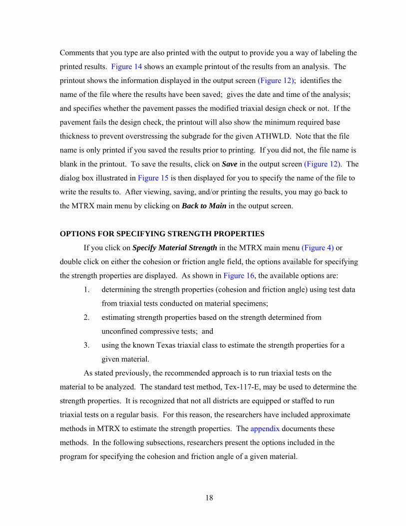
Comments that you type are also printed with the output to provide you a way of labeling the
printed results. Figure 14 shows an example printout of the results from an analysis. The
printout shows the information displayed in the output screen (Figure 12); identifies the
name of the file where the results have been saved; gives the date and time of the analysis;
and specifies whether the pavement passes the modified triaxial design check or not. If the
pavement fails the design check, the printout will also show the minimum required base
thickness to prevent overstressing the subgrade for the given ATHWLD. Note that the file
name is only printed if you saved the results prior to printing. If you did not, the file name is
blank in the printout. To save the results, click on Save in the output screen (Figure 12). The
dialog box illustrated in Figure 15 is then displayed for you to specify the name of the file to
write the results to. After viewing, saving, and/or printing the results, you may go back to
the MTRX main menu by clicking on Back to Main in the output screen.
OPTIONS FOR SPECIFYING STRENGTH PROPERTIES
If you click on Specify Material Strength in the MTRX main menu (Figure 4) or
double click on either the cohesion or friction angle field, the options available for specifying
the strength properties are displayed. As shown in Figure 16, the available options are:
1. determining the strength properties (cohesion and friction angle) using test data
from triaxial tests conducted on material specimens;
2. estimating strength properties based on the strength determined from
unconfined compressive tests; and
3. using the known Texas triaxial class to estimate the strength properties for a
given material.
As stated previously, the recommended approach is to run triaxial tests on the
material to be analyzed. The standard test method, Tex-117-E, may be used to determine the
strength properties. It is recognized that not all districts are equipped or staffed to run
triaxial tests on a regular basis. For this reason, the researchers have included approximate
methods in MTRX to estimate the strength properties. The appendix documents these
methods. In the following subsections, researchers present the options included in the
program for specifying the cohesion and friction angle of a given material.

19
Figure 14. Example Printout of Analysis Results from MTRX.

20
Figure 15. Dialog Box to Save Results from MTRX.
Figure 16. Options for Specifying Strength Properties in MTRX.

21
Determining Strength Properties from Available Triaxial Test Data
If you conducted triaxial tests, click on Triaxial Test Data in the menu given in
Figure 16 to use the program in determining the cohesion and friction angle. To use this
option, you will need to have the compressive strengths determined at two or more confining
pressures. After you click on Triaxial Test Data, MTRX displays the form shown in
Figure 17. Specify the layer number of the material on which you conducted triaxial tests.
For the subgrade, this would be “3” or “4” depending on whether you are analyzing a three-
or four-layer pavement. Note that the layer number should correspond to the subgrade or to
the base (if you use the Check Base option). If you specify an invalid layer number, the
program will notify you. The program automatically sets the layer to the number for the
subgrade when the Check Base option is not selected in the main menu.
There are seven buttons at the bottom of the form shown in Figure 17. The Input
data button allows you to enter corresponding values of confining pressure and failure stress.
To do this, type a value of lateral pressure in the Confining pressure field and the
corresponding value of the failure stress in the Load at failure field. Then, click on Input
data to accept your entries. The corresponding data pair is then displayed under the
Confining pressure and Failure stress columns of the form. Repeat this sequence for other
pairs of triaxial test data until you have entered all data.
You may save your input by clicking on Save data in the form shown in Figure 17.
Likewise, you may load an existing triaxial data file by clicking on Load data. The file
Example Subgrade Triaxial Data.TXT that is copied to the MTRX program subdirectory
during installation is a sample triaxial data file that you may use in learning the operation of
this function for determining strength properties. This file contains data from Texas triaxial
tests conducted on sandy clay subgrade specimens molded from material taken along FM 782
in Rusk County to evaluate a superheavy load move. The sample data shown in Figure 17
were read from this file.
The Clear a row or Clear all buttons allow you to edit the data displayed in the menu.
To clear a pair of confining pressure and failure stress previously entered, highlight the
record by clicking on either one of these items. Then click on Clear a row to delete the
highlighted data pair. To delete all data, click on the Clear all button.

22
Figure 17. Form to Enter Compressive Strengths at Different Confining Pressures.
Once you have entered all triaxial test data, you may click on C & Angle to determine
the cohesion and friction angle of the material. The results of the calculations are presented
in the output screen illustrated in Figure 18 where the Mohr’s circles and the failure envelope
are plotted. Click on Print to get a hardcopy of the chart shown. When you are finished
viewing the results, click on Back to return to the form shown in Figure 17. From here, you
may evaluate the strength properties of another material or return to the main menu by
clicking on the Back button of the form. The main menu displays the cohesion and friction
angle determined from the analysis of triaxial test data.
Estimating Strength Properties from Unconfined Compressive Strength (UCS)
As indicated in Figure 16, options for estimating the strength properties based on
UCS are grouped according to whether the material is stabilized or unstabilized. It is

23
Figure 18. Determining Failure Envelope from Triaxial Test Data.
emphasized that these methods are approximate and were developed based on information
obtained from the literature. You may use the methods for stabilized materials to evaluate
pavement designs that incorporate asphalt-, lime-, or cement-treated base materials when the
Check Base option is selected in the main menu. Note that these methods are only used to
estimate the strength properties of stabilized materials for the case where you want to
evaluate the potential of overstressing the base for the given pavement and load. Otherwise,
the strength properties of the base layer are not necessary to run the program.
Click on Unconfined Compressive Strength (UCS) in the screen shown in Figure 16
to use the options for stabilized materials (note that you must first select the Stabilized option
in the screen shown in Figure 16). The dialog box shown in Figure 19 is then displayed for
you to specify the type of stabilized material to be evaluated. If the material is asphalt-
stabilized, click on Asphalt Stabilized in the dialog box and specify the layer number and the
UCS for the material. Note that you only need to specify the layer number if you selected the
Check Base option in the main menu. If you did not select Check Base, the program
automatically sets the number to that of the subgrade layer.
When you have entered the UCS, click on Accept to confirm your entries and
estimate the cohesion. For asphalt-stabilized base layers, the friction angle is assumed to be
zero in determining the cohesion from the UCS. This approximation is used since the lower

24
Figure 19. Illustration of Asphalt-Stabilized Option for Estimating StrengthProperties.
part of the asphalt-stabilized base will most likely be in tension. This means that very little
of the interparticle friction is mobilized. For N = 0°, the cohesion is simply 1⁄2 × UCS.
If the material is lime-stabilized and the UCS is known, click on Lime-stabilized.
The dialog box shown in Figure 20 is displayed where you need to specify the layer number
and the UCS for the lime-treated material. For these materials, the friction angle typically
varies between 25 to 35 degrees (Little, 1995). A default value of 30°, is used but you may
specify another angle by sliding the pointer in the dialog box to the value you wish to use, or
by typing in the friction angle in the cell provided. Note that the friction angle for lime-
stabilized materials is limited to be within the range of 25° to 35° in the method used to
estimate strength properties for this material. Click on Accept to confirm your entries. The
cohesion of soil-lime mixtures is estimated as 30 percent of the UCS (Little, 1995).
If the material is cement-treated and the UCS is known, you may characterize the
layer as following either the Griffith or modified Griffith criterion (Raad, Monismith, and
Mitchell, 1977). The application of these criteria to estimate the strength properties of
cement-treated materials is explained in the appendix (in the section on stabilized materials
on pages 45 to 48). Click on Cement-treated, and specify the criterion to use in the dialog
box shown in Figure 21. Enter the layer number and UCS of the cement-treated material,
then click on Accept. Note that the strength properties depend on the confining pressure for

25
Figure 20. Illustration of Lime-Stabilized Option for Estimating Strength Properties.
Figure 21. Illustration of Cement-Treated Option for Estimating Strength Properties.

26
a material that behaves according to the Griffith criterion. For this reason, the cohesion and
friction angle will vary within a layer so that these properties are predicted at each point
where the Mohr-Coulomb yield function is evaluated. Note that the main menu will display
–9.000 in the fields for cohesion and friction angle. This only identifies the material as
following the Griffith criterion. The strength properties are actually predicted during run
time of the analysis module of MTRX (when the triaxial design check is performed). If you
want to see the predicted values of cohesion and friction angle, you need to save the results
from the analysis as discussed previously. You may then open this output file in a word
processor or editor (such as Notepad©) to view the strength properties as well as the
predicted values of the Mohr-Coulomb yield function at the different evaluation positions.
If the material is unstabilized, click Unstabilized in the menu shown in Figure 16.
Then, click on Unconfined Compressive Strength (UCS) to view the dialog box (Figure 22)
for estimating the strength properties of unstabilized materials. To estimate the cohesion and
friction angle for these materials, you may either specify the unconfined compressive
strength or the strength at another confining pressure. The latter option is provided for
evaluating weak materials that may prove difficult to test at zero confining pressure.
In the dialog box, specify the layer number of the material to be characterized, its
TTC and the UCS (if known). The TTC should be between 0.5 and 6.5. This material
classification is used to estimate the compressive strength at 5 psi (S5) from the following
relationship developed by Scrivner and Moore (1967):
S5 = 9.3 + 0.4539 × (8 – TTC)3 (6)
The predicted compressive strength at 5 psi is displayed in the dialog box when you
enter the TTC of the material. This is illustrated in Figure 22. Given S5 and the compressive
strength at another confining pressure, the strength properties of unstabilized materials are
estimated in MTRX. If you know the UCS, click Only UCS in the dialog box and enter the
UCS in the space provided. You also may specify the compressive strength at another
confining pressure by clicking Strength at another confining pressure in the dialog box and
entering the required data in the fields for F1 and F3 shown in Figure 23. Note that the

27
Figure 22. Estimating Strength Properties of Unstabilized Materials from UCS.
Figure 23. Specifying the Compressive Strength at Another Confining Pressure.

28
compressive strength F1 must be for a confining pressure F3 other than 5 psi. This option is
provided for the case where the material is too weak to test at zero confining pressure to get
the UCS.
When you have entered the required information, click on Accept in the dialog box to
confirm your entries and to estimate the cohesion and friction angle for the unstabilized
material. You may then characterize the strength properties of another layer or return to the
main menu by clicking on Back in the dialog box. The strength properties determined for the
layer you characterized are displayed in the main menu.
Estimating Strength Properties Based on Texas Triaxial Class
If triaxial test data and the UCS are not available, MTRX provides an option to
estimate the strength properties from the known Texas triaxial class of the material. To
access this function, click on Use Texas Triaxial Class (TTC) in the screen shown in
Figure 16. This brings up the chart in Figure 24 that shows the linearized forms of the TTC
failure envelopes from the provisional Test Method Tex-143-E. TxDOT developed this test
method in-house but has not formally adopted it at the time of this report. The linearized
boundaries between classes were determined by fitting a line to each of the class boundaries
in the standard Test Method Tex-117-E classification chart.
In the approximate method described herein, the linearized class boundaries in
Figure 24 are used to interpolate the failure envelope corresponding to the prescribed TTC.
This interpolation is done such that the TTC is maintained at each point on the failure
envelope. Figure 24 illustrates this approach where the dashed line corresponds to the
interpolated failure envelope for a TTC of 4.8.
To interpolate the failure envelope after specifying the TTC for the layer to analyze,
click on C & Angle at the bottom of the chart to estimate the cohesion and friction angle for
the material. Click on Back to return to the main menu where the strength properties are
displayed.
NONLINEAR ANALYSIS OPTION
As mentioned earlier, MTRX provides the option of modeling the nonlinear behavior
observed in most pavement materials. This capability becomes particularly important for
thin pavements, which comprise a big portion of the highway network in Texas. For these

29
Figure 24. Estimating Strength Properties Using TTC and Tex-143-E ClassificationChart.
pavements, a nonlinear analysis will provide a more realistic prediction of the stresses
induced under loading (Jooste and Fernando, 1995). This analysis in MTRX uses the
following equation by Uzan (1985) to model stress-dependency:
(7)E K paIpa pa
Koct
K
=⎛⎝⎜
⎞⎠⎟
⎛⎝⎜
⎞⎠⎟1
12 3τ
where,
E = layer modulus,
I1 = first stress invariant determined from Eq. (3),
Joct = octahedral shear stress,

30
pa = atmospheric pressure (14.5 psi), and
K1, K2, K3 = material constants determined from resilient modulus testing.
The octahedral shear stress may be determined from the second deviatoric stress
invariant J2 computed from Eq. (4). The relationship between Joct and J2 is given by:
(8)τ oct J=23 2
The material constants of Eq. (7) may be characterized following AASHTO T-292 for
unstabilized materials and ASTM D 3497 for asphalt-stabilized materials. K2 is typically
positive, indicating increased stiffness at higher confinement, while K3 is typically negative,
indicating a stiffness reduction with increased deviatoric stress. To use the nonlinear
analysis option in MTRX, these constants must be characterized. No approximate methods
have been incorporated in this version of the analysis program, although Glover and
Fernando (1995) present relationships for estimating these resilient properties based on
Atterberg limits, gradation, and soil suction measurements made on unstabilized materials.
If you want to use the nonlinear option for a particular project and you have the K1,
K2, and K3 coefficients for the stress-dependent pavement material(s), click Nonlinear in the
main menu given in Figure 4. Cells for entering the coefficients are then displayed in the
menu as illustrated in Figure 25. By default, the K2 and K3 values are initially set to zero
corresponding to linear behavior, i.e., the modulus is independent of stress as inferred from
Eq. (7). In this case, K1 is simply calculated by dividing the specified modulus of the
material by the atmospheric pressure of 14.5 psi. The resulting value is displayed in the main
menu as shown in Figure 25.
Enter the coefficients for the nonlinear pavement layer(s) in the main menu. If you
want to model a layer as linear, simply leave the initial values as they are, i.e., K2 = K3 = 0,
and K1 equal to the layer modulus divided by14.5 psi. You then may continue entering other
input data as described in this manual or run an analysis as appropriate.

31
Figure 25. Specifying K1, K2, and K3 Coefficients for Nonlinear Analysis in MTRX.
THE LEAST YOU NEED TO KNOW
To summarize, conducting a triaxial design check using MTRX will require that you
at least know the following:
1. modulus, Poisson’s ratio, and thickness of each pavement layer;
2. average of the ten heaviest wheel loads; and
3. Texas triaxial class of the subgrade.
The above data represent the minimum that are required to run MTRX. You may obtain
these data from the flexible pavement design. Note that running the program and getting
good results are two different things. To do an adequate analysis, you should know the
properties of your materials and model the pavement realistically. Good engineering practice
will require that you make the effort to search published information, review past experience,
and/or run tests to characterize the materials for a given problem.


33
CHAPTER III
SUMMARY AND RECOMMENDATIONS
The preceding chapter explained the operation of the MTRX program to evaluate the
structural adequacy of pavement designs based on the Mohr-Coulomb yield criterion. In the
opinion of the researchers, the development of this program is a significant step toward
improving the existing Texas modified triaxial design check. Among the capabilities that the
program provides are:
1. input of design layer moduli and thicknesses from FPS to perform the design
check;
2. characterization of pavement layers as linear materials with constant moduli or
as nonlinear materials with stress-dependent moduli that obey the constitutive
relationship given by Eq. (7); and
3. modeling of steering, single, and tandem axle configurations.
Since MTRX permits the user to directly input the material properties of each layer,
TxDOT engineers will have the capability to model their particular environmental conditions
and local materials. Thus, districts in west Texas will have the option of conducting an
analysis using strength properties that correspond to in-situ moisture conditions in lieu of
properties obtained under capillary saturation. Similarly, stabilized materials are
characterized using modulus and strength properties instead of cohesiometer values that give
only an indication of the strength of the material and are rarely characterized by the districts.
Finally, MTRX permits pavement engineers to directly model the effects of different axle
configurations on pavement response in lieu of applying a safety factor of 1.3 to the
ATHWLD when there are more than 50 percent tandem axles in the traffic stream.
In the evaluation of structural adequacy, the Mohr-Coulomb yield criterion is checked
at a number of positions within the pavement corresponding to the top, middle, and bottom of
the base layer, and the top of the subgrade. At each of these depths, the stresses under load
are predicted at different lateral offsets corresponding to the outside tire edge, middle of the
tire, inside tire edge, and midway between dual tires as illustrated in Figure 26. Additionally,

34
Figure 26. Locations where Stresses are Predicted for Evaluating StructuralAdequacy.
for tandem axles, the stresses at the same positions are evaluated midway between the axles.
At each evaluation position, the stresses are used with the Mohr-Coulomb strength properties
to predict if overstressing will occur for the given pavement and design load.
While the development of MTRX represents a significant step toward updating the
existing methodology to be more consistent with the mechanistic-empirical design
philosophy that underpins FPS, much more work needs to be done to realize the potential
benefits that implementation of this program may bring. Toward this end, the authors offer
the following recommendations for further research:
1. The Mohr-Coulomb failure envelopes in the existing flexible base design chart
used in Tex-117-E show a nonlinear relationship between failure stress and
confining pressure. This nonlinear relationship has been observed in laboratory
tests conducted by Lu, Shih, and Scrivner (1973) for stabilized and unstabilized
base materials. The form of this relationship is expressed in Eq. (18) of the

35
appendix, which gives the model used in MTRX to characterize the Griffith
criterion for cement-treated materials. The authors recommend an evaluation to
verify the applicability of this model to other pavement materials. This
evaluation should include a review of triaxial test data collected in previous
TxDOT projects, as well as an extensive laboratory program to characterize
strength properties for stabilized and unstabilized materials used by the
department.
2. Before laboratory tests are carried out, researchers should initially develop a test
plan that will identify the types of materials to be tested, the factors that will be
included in the experiments, and the measurements to be made. The effect of
moisture content on the Mohr-Coulomb strength properties should be
investigated to develop guidelines for characterizing these properties that
consider the different environmental regions of the state. The authors also
recommend that the laboratory program include characterizations of the stress-
dependent behavior of the materials to be tested. The results from these tests
will be useful in developing procedures to establish the K1, K2, and K3
coefficients of Eq. (7) for implementing the nonlinear analysis option in MTRX.
In view of the upcoming release of the 2002 American Association of State
Highway and Transportation Officials (AASHTO) pavement design guide, the
resilient modulus tests proposed herein may also be conducted as part of a
larger effort of evaluating and implementing the AASHTO 2002 pavement
design procedure within TxDOT.
3. The options available in MTRX for estimating strength properties should be
updated accordingly based on analysis of the triaxial data collected from the
laboratory test program. In addition, the program should be updated to include
options for estimating the stress-dependent material parameters for the
nonlinear analysis.
4. A pilot implementation program should be conducted in selected districts to
introduce MTRX to TxDOT pavement design engineers who are expected to be
the primary users of this analysis procedure. The authors recommend that this
implementation be conducted on actual projects where demonstrations are

36
provided that show how test data needed for the design check are established.
In addition, training on the application of the MTRX program should be
provided.

37
REFERENCES
Chen, W. F. and G. Y. Baladi. Soil Plasticity, Theory and Implementation. Developments in
Geotechnical Engineering, Vol. 38, Elsevier, New York, 1985.
Glover, L. T. and E. G. Fernando. Evaluation of Pavement Base and Subgrade Material
Properties and Test Procedures. Research Report 1335-2, Texas Transportation Institute,
Texas A&M University, College Station, Texas, 1995.
Jooste, F. J. and E. G. Fernando. Development of a Procedure for the Structural Evaluation
of Superheavy Load Routes. Research Report 1335-3F, Texas Transportation Institute, Texas
A&M University, College Station, Texas, 1995.
Little, D. N. Handbook For Stabilization of Pavement Subgrades and Base Courses With
Lime. Kendall/Hunt Publishing Company, Iowa, 1995.
Lu, D. Y., C. S. Shih, F. H. Scrivner. The Optimization of a Flexible Pavement System Using
Linear Elasticity. Research Report 123-17, Texas Transportation Institute, Texas A&M
University, College Station, Texas, 1973.
Raad, L., C. L. Monismith, and J. K. Mitchell. Fatigue Behavior of Cement-Treated
Materials. In Transportation Research Record 641, TRB, National Research Council,
Washington, D. C., 1977, pp. 7S11.
Scrivner, F. H. and W. M. Moore. Some Recent Findings in Flexible Pavement Research.
Research Report 32-9, Texas Transportation Institute, Texas A&M University, College
Station, Texas, 1967.
Scrivner, F. H. and W. M. Moore. A Tentative Flexible Pavement Design Formula and Its
Research Background. Research Report 32-7, Texas Transportation Institute, Texas A&M
University, College Station, Texas, 1966.

38
Uzan, J. Granular Material Characterization. In Transportation Research Record 1022,
TRB, National Research Council, Washington, D. C., 1985, pp. 52–59.

39
APPENDIX
PROCEDURES FOR SPECIFYING STRENGTH PROPERTIES
To perform a design check using the MTRX program, the user must specify the
cohesion and friction angle that define the Mohr-Coulomb failure envelope and the Texas
triaxial class of a given material. The authors recommend that these properties be
determined from triaxial tests on the materials selected for designing and constructing a
given pavement. For this determination, you may use MTRX to get the strength properties
from triaxial test data as presented in Chapter II of this report. However, the authors
recognize that data from laboratory tests will not always be available for determining the
strength properties that are input to the analysis program. To facilitate implementation, the
authors included a number of options in MTRX that the engineer may use to specify these
properties. These options, which were developed using results from previous investigations,
are described in the following.
RELATIONSHIP BETWEEN TEXAS TRIAXIAL CLASS AND COMPRESSIVE
STRENGTH
Using data from triaxial tests conducted by the Bryan District on 106 pavement
materials, Scrivner and Moore (1967) developed the following relationship between the
Texas triaxial class and the compressive strength at a confining pressure of 5 psi:
S5 = 9.3 + 0.4539 (8 !TTC)3 (9)
where,
S5 = predicted compressive strength in psi, and
TTC = Texas triaxial class restricted to the interval, 0.5 # TTC # 6.5.
Figure 27 shows how the above relationship fits the triaxial test data. Scrivner and Moore
(1967) did not report goodness-of-fit statistics for Eq. (9). However, it is observed from
Figure 27 that the equation fits the data points quite well. Moreover, Scrivner and Moore
conducted an independent verification of Eq. (9) using additional data from triaxial tests

40
Figure 27. Relationship between TTC and Compressive Strength at 5 psi ConfiningPressure from Tests Conducted by Bryan District (Scrivner and Moore,1967).

41
done on 113 different materials obtained from 13 districts. Figure 28 shows how the
equation fits the additional data obtained. Note that the data points shown in the figure were
not used in developing Eq. (9). Considering the reasonable fit, Figure 28 indicates that
Eq. (9) is fairly robust.
While an estimate of TTC may be obtained from Eq. (9) given S5, using the equation
in an inverse manner is not recommended. Equation (9) is derived by curve fitting laboratory
data so that the coefficients of the equation depend on the choice of independent and
dependent variables. Also, note that the equation is valid for TTCs within the range of 0.5 to
6.5. Compressive strengths determined for TTCs outside this range represent extrapolated
values.
It is also noted that Figures 27 and 28 include data points where the TTCs are below
2.0. These values were obtained using the special classification chart shown (Figure 29) that
includes a line for Class 1 materials derived by Scrivner and Moore (1966) from
extrapolation of the lines for Class 2, 3, 4, and 5 materials. Researchers used the Class 1
curve shown in Figure 29 to add a Class 1 line to the linearized classification chart used in
MTRX to estimate the Mohr-Coulomb strength properties given the TTC.
Equation 9 is applicable for unstabilized materials. Knowing the compressive
strength, the Mohr’s circle for a confining pressure of 5 psi may be constructed. However, to
determine the cohesion and friction angle, the Mohr’s circle at an additional confining
pressure is needed. If the unconfined compressive strength of the material is known, these
properties may be estimated from the following relations, which the researchers derived
using Mohr-Coulomb failure theory:
(10)φ =− +− −
⎛⎝⎜
⎞⎠⎟−Sin
UCS SUCS S
1 5
5
55
and
(11)cUCS
=−sin ( sin )
sinφ φ
φ1
2
where,

42
Figure 28. Verification of Relationship for Predicting Compressive Strength at 5 psiConfining Pressure Using Data from Other Districts (Scrivner andMoore, 1967).

43
Figure 29. Texas Triaxial Classification Chart with Class 1 Line (Scrivner and Moore,1967).

44
N = friction angle,
c = cohesion, psi,
UCS = unconfined compressive strength (psi), 0 # UCS # (S5 - 5), and
S5 = predicted compressive strength at 5 psi confining pressure from
Eq. (9).
The unconfined compressive strength may be obtained from previous data or from
actual laboratory tests. For weak materials (Class 5 and lower) it may be difficult to run a
test at zero confining pressure to determine the UCS. For these unstabilized materials, it may
be necessary to apply a confining pressure to determine the Mohr’s circle of stress. In this
instance, if the applied confining pressure is denoted as F3, and the compressive strength
determined from the test is denoted as F1, the strength properties are determined from the
following relations:
(12)φσ σσ σ
=− − −+ − +
⎡
⎣⎢
⎤
⎦⎥
−SinSS
1 1 3 5
1 3 5
55
( ) ( )( ) ( )
and
(13)c =− − +σ φ φ σ φ φ
φ1 31 1
2sin ( sin ) sin ( sin )
sin
where the terms are as defined previously. Note that Eqs. (12) and (13) reduce to Eqs. (10)
and (11) respectively at zero confining pressure (F3 = 0) for which F1 = UCS. Equations (9),
(10), and (11) may be used to estimate the Mohr-Coulomb strength properties of unstabilized
materials given the TTC and UCS, while Eqs. (9), (12), and (13) are used if the TTC and the
failure stress from a triaxial test conducted at another confining pressure (F3 … 0 and F3 … 5
psi) are available.
Note that the cohesion and friction angle of unstabilized soils are influenced by
moisture content. Since the TTC in Eq. (9) is determined from tests on soil specimens that
have undergone capillary saturation, the compressive strength at the other confining pressure
must also be determined under the same moisture condition for the strengths to be
comparable. Thus, the cohesion and friction angle determined using Eqs. (9), (10), and (11),
or Eqs. (9), (12), and (13) are based on capillary saturated specimens consistent with Test
Method Tex-117-E.

45
STABILIZED MATERIALS
The unconfined compressive strength may be used in evaluating the load carrying
capacity of stabilized materials. In the absence of laboratory triaxial test data, one approach
that may be used for asphalt-stabilized layers is to assume the friction angle to be zero (N = 0
condition) and compute the cohesion as:
c = 1⁄2 UCS (14)
For stabilized base materials, the critical region will likely be at the bottom of the base
underneath the load where tensile stresses are likely to be induced. Under this condition, the
strength attributed to interparticle friction will likely be minimal since the material is being
pulled apart. Thus, the load carrying capacity will depend, to a large extent, on the cohesion
of the material. From this perspective, there is a rationale for using the above approach to
evaluate the load carrying capacity of asphalt-stabilized materials in the absence of triaxial
test data. The laboratory test program recommended in Chapter III should provide data that
can be used to verify this approach.
For soil-lime mixtures, the major effect of lime stabilization is to increase the
cohesion of the material (Little, 1995). The cohesion is observed to increase with mixture
compressive strength and may be roughly approximated at 30 percent of UCS. Some minor
increase in the friction angle is observed with lime stabilization. For these materials, the
friction angle typically varies from 25° to 35°.
For cement-stabilized materials, the Griffith criterion has been proposed to
characterize the relationship between failure stress and confining pressure. Figure 30 shows
triaxial test data for a number of cement-treated materials. The data were obtained from
triaxial tests on soil cements used in pavement base layers, embankments, and dams and
from tests conducted on concrete materials under biaxial loading conditions. It is observed
that the data points appear to follow a fairly well-defined trend when the failure stress and
confining pressure are normalized by the unconfined compressive strength denoted by the
symbol, Func, in Figure 30. Also shown are two criteria that have been proposed to model the
relationship between failure stress and confining pressure for cement-treated materials.
These criteria are the Griffith and the modified Griffith criteria. Most of the data points in
Figure 30 are observed to follow the modified Griffith criterion, which is defined by the
following linear equation:

46
Figure 30. Normalized Failure Envelopes for Cement-Treated Soils (Raad,Monismith, and Mitchell, 1977).

47
F1' = $0 + $1 F3' (15)
where,
F1' = F1/Func,
F3' = F3/Func,
Func = unconfined compressive strength (UCS),
F3 = applied confining pressure in the triaxial test,
F1 = measured failure stress corresponding to F3, and
$0, $1 = model coefficients.
Using Eq. (15), researchers derived the following relationships for estimating N and c for
cement-stabilized materials following Mohr-Coulomb failure theory:
(16)φββ
=−+
⎛⎝⎜
⎞⎠⎟−Sin 1 1
1
11
and
(17)cUCS
=β
β0
12
From Figure 30, the coefficients of the modified Griffith criterion are determined to
be $0 . 0.9 and $1 . 6. Thus, based on the modified Griffith criterion, the failure envelopes
for cement-treated materials are a family of lines of constant slope, N . 45.6°, with
y-intercepts or cohesion values that are approximated by c . 0.18 UCS. Physically, this
means that the Mohr’s circles of stress expand in proportion to the unconfined compressive
strength of the material consistent with the linear relationship assumed in Eq. (15).
The Griffith criterion in Figure 30 defines a lower boundary of the data plotted in the chart.
For a given confining pressure, the Griffith criterion will predict a lower failure stress than
the modified criterion given in Eq. (15) and is, thus, more conservative. The following
model may be used to define the nonlinear relationship between failure stress and confining
pressure that is assumed in the Griffith criterion:
(18)σ ασα
α
1 03
11
2
''
= +⎛
⎝
⎜⎜
⎞
⎠
⎟⎟

48
where, "0, "1, and "2 are model coefficients and the other terms are as defined previously.
The coefficients "0, "1, and "2 are 1.0, 0.125, and 0.462, respectively. Researchers
determined these coefficients by digitizing the Griffith curve in Figure 30 and fitting Eq. (18)
to the digitized points by nonlinear regression. The root-mean-square error of the fitted
curve from the regression is 0.009 with 123 digitized points.
Equation (18) reduces to F1 = Func = UCS when the confining pressure, F3 = 0. Also,
it may be discerned from Eq. (18) and Figure 30 that "1 × UCS is an estimate of the tensile
strength of the material. If Eq. (18) is used to model Griffith’s criterion, the following
equations for estimating friction angle and cohesion are determined:
(19)φ =−+
⎛⎝⎜
⎞⎠⎟−Sin
AA
1 11
where,
(20)A = +⎛⎝⎜
⎞⎠⎟
−α αα
σα
α0 2
1
3
1
1
12'
and,
(21)cUCS
=⎛⎝⎜
⎞⎠⎟ +
⎛⎝⎜
⎞⎠⎟ −
⎛⎝⎜
⎞⎠⎟ +
⎛⎝⎜
⎞⎠⎟
⎡
⎣
⎢⎢⎢
⎤
⎦
⎥⎥⎥
+ −
21 10 1
2
1 23
1
12
30 2
1
1 23
1
12
2 2
α αα
σα
σα αα
σα
α α/ /
''
'
The nonlinear relationship between failure stress and confining pressure has been observed in
laboratory tests conducted by Lu, Shih, and Scrivner (1973) for stabilized and unstabilized
materials. Because of this, the resulting failure envelope is also nonlinear so that Eqs. (19) to
(21) define the tangent to the failure envelope at a given confining pressure.
GRAPHICAL METHODS
If the TTC and the cohesion or friction angle of a material are known, the failure
envelope may be uniquely determined using the classification chart shown in Figure 29.

49
In certain cases, however, the only information that may be known about a material is its
Texas triaxial class. The TTC is determined by overlaying the failure envelope on the chart
shown in Figure 29 and locating the point on the envelope farthest from the upper class line.
However, given only the TTC, it is not possible to uniquely determine the failure envelope
since any number of lines may be made to pass the point. To provide an approximate method
to evaluate structural adequacy, assumptions must be made to interpolate a failure envelope
from the classification chart, given only the Texas triaxial class. In the approximate
procedure used in MTRX, the class lines in Figure 29 are linearized as illustrated in
Figure 31. In this figure, the solid lines represent the classes included in the classification
chart given in Test Method Tex-117-E. The dashed lines are the linearized class boundaries
that are proposed in the new triaxial test method designated as Tex-143-E. MTRX uses these
linearized class boundaries to interpolate the failure envelope corresponding to a prescribed
Texas triaxial class. This interpolation is done such that the specified TTC is maintained at
each point on the failure envelope as illustrated in Figure 24. MTRX then uses the
interpolated envelope to predict if overstressing of the material will occur for the prescribed
loading and pavement structure.
TRIAXIAL TESTING OF PAVEMENT MATERIALS
While the previous sections have presented methods for estimating the strength
properties of pavement materials, the authors recommend direct characterization of the
failure envelope from laboratory tests. This characterization may be done following
Tex-117-E or the provisional procedure designated as Tex-143-E once TxDOT formally
adopts it. In this latter method, the specimen is encased in an elastic membrane and placed
inside an acrylic cell that can be filled with water or air for application of the confining
pressure. Typically, specimens are tested at confining pressures of 3, 7, and 10 psi. Given
the failure stresses at different confining pressures, the failure envelope may be determined
through a numerical procedure that finds the cohesion and friction angle values, c and N,
resulting in the best fit to the following equation:
(22)σσ
φ φ σσ φ
1
3
3
3
2 11
=+ +−
ccos ( sin )( sin )

50
Figure 31. Linear Regression Lines Fitted to Tex-117E TTC Curves.
where the corresponding pairs of failure stresses (F1) and confining pressures (F3) are
determined from the tests. At the very least, triaxial tests must be done at two confining
pressures. For this case, if the failure stresses, corresponding to confining pressures of F3
and F3', are denoted as F1 and F1', respectively, the Mohr-Coulomb strength properties are
determined directly from the following equations:
(23)φσ σ σ σσ σ σ σ
=− − −+ − +
⎡
⎣⎢
⎤
⎦⎥
−Sin 1 1 3 1 3
1 3 1 3
( ) ( ' ' )( ) ( ' ' )
and
(24)c =− − +σ φ φ σ φ φ
φ1 31 1
2sin ( sin ) sin ( sin )
sin

51
SUMMARY
This appendix presented different options for characterizing the failure envelopes of
pavement materials that MTRX requires to evaluate structural adequacy. In this new
program, the stresses induced under load are predicted using a layered elastic pavement
model, which permits a linear or nonlinear characterization of pavement materials. Steering,
single, and tandem axle configurations may be modeled directly in the computer program.
The predicted stresses at critical locations within the base and subgrade layers are
checked against the Mohr-Coulomb yield criterion to evaluate whether the given pavement
will sustain a single application of the prescribed load without undergoing a rapid shear
failure. This approach is consistent with the theoretical basis for the existing modified
triaxial design procedure. Note that the development of permanent deformation due to
repeated traffic loading is not considered in this design check nor in the current FPS-19
design program. The researchers recommend that future work incorporate this distress mode
as a design criterion in FPS.
To evaluate the potential for rapid shear failure under a single load application, the
failure envelopes of the base and subgrade materials are specified through input of the
cohesion and friction angle values. It is emphasized that these properties are influenced by
moisture content. Consequently, it is important to characterize these properties for the
expected in-service conditions, which range from dry to wet as one goes from west to east
Texas.
MTRX incorporates the options presented in this appendix for determining or
estimating the Mohr-Coulomb strength parameters. Table 1 summarizes the available
options, while Figure 32 shows a flowchart of the computer program. Future work should
include laboratory tests to verify the options presented for estimating the strength properties,
particularly for the stabilized materials used in the state for which very limited triaxial test
data are available.

52
Table 1. Options for Specifying Mohr-Coulomb Strength Properties.
Condition Option
A. Triaxial test data at two or moreconfining pressures are available:
Use Eq. (22) to find N and c given thefailure stresses at three or more confiningpressures, or Eqs. (23) and (24) if triaxialtest data are available at only two confiningpressures.
B. If there are no triaxial test data attwo or more confining pressures,then:
If material is unstabilized and theUCS is known or triaxial test data atanother confining pressure areavailable:
Use Eqs. (10) and (11) to estimate N and c,respectively, given the UCS, or Eqs. (12)and (13) if triaxial test data at anotherconfining pressure are available.
If material is asphalt stabilized: Assume N = 0 and estimate cohesion fromEq. (14); or
If lime stabilized and UCS isknown:
Assume N between 25° and 35° andestimate c . 0.30 UCS
If cement-treated and UCS isknown:
Assume the modified Griffith criterion anduse Eqs. (16) and (17) to estimate strengthproperties, or assume the Griffith criterionand use Eqs. (19), (20), and (21).
C. If triaxial test data and UCS are notavailable, then:
If only TTC is known Interpolate failure envelope using linearizedclass boundaries from Tex-143-E

53
Figure 32. Flowchart of Options for Specifying Mohr-Coulomb Strength Propertiesin MTRX.

54
Figure 32. Flowchart of Options for Specifying Mohr-Coulomb Strength Properties inMTRX (continued).


