The surprising robustness of dynamic Mean-Variance ...
31
The surprising robustness of dynamic Mean-Variance portfolio 1 optimization to model misspecification errors 2 Pieter M. van Staden Duy-Minh Dang Peter A. Forsyth 3 November 12, 2021 4 Abstract 5 In single-period portfolio optimization settings, Mean-Variance (MV) optimization can result 6 in notoriously unstable asset allocations due to small changes in the underlying asset parameters. 7 This has resulted in the widespread questioning of whether and how MV optimization should be 8 implemented in practice, and has also resulted in a number of alternatives being proposed to the 9 MV objective for asset allocation purposes. In contrast, in dynamic or multi-period MV portfo- 10 lio optimization settings, preliminary numerical results show that MV investment outcomes can 11 be remarkably robust to model misspecification errors, which arise when the investor derives an 12 optimal investment strategy based on some chosen model for the underlying asset dynamics (the 13 investor model), but implements this strategy in a market driven by potentially completely dif- 14 ferent dynamics (the true model). In this paper, we systematically investigate the causes of this 15 surprising robustness of dynamic MV portfolio optimization to model misspecification errors under 16 both the pre-commitment MV (PCMV) and time-consistent MV (TCMV) approaches. We identify 17 particular combinations of parameters that play a key role in explaining the observed model mis- 18 specification errors. We investigate the impact of the chosen dynamic MV approach, underlying 19 model formulation, portfolio rebalancing frequency and the application of multiple realistic invest- 20 ment constraints on the robustness of investment outcomes, as well as the implications for model 21 calibration. 22 Keywords: Asset allocation, constrained optimal control, time-consistent, mean-variance 23 AMS Subject Classification: 91G, 65N06, 65N12, 35Q93 24 1 Introduction 25 Mean-variance (MV) portfolio optimization, originating with Markowitz (1952), has become the foun- 26 dation of modern portfolio theory (Elton et al. (2014)). MV investment strategies are appealing due 27 to their intuitive nature, since they clearly illustrate the trade-off between reward (expected return) 28 and risk (variance of returns). 29 In single-period settings, MV optimization can provide notoriously unstable asset allocations aris- 30 ing from small changes in the underlying asset parameters (Michaud and Michaud (2008)). This issue 31 has become especially pressing in recent machine learning applications (see for example Sato (2019)), 32 where the use of “robo-advisors” for automatic portfolio allocation may in fact require significant 33 human intervention to compensate for this sensitivity of MV portfolio allocations (Bourgeron et al. 34 (2018); Perrin and Roncalli (2019)). 35 In order to increase the robustness of single-period MV asset allocations to changes in the under- 36 lying parameters, two fundamental approaches can be distinguished in the literature: (i) adjusting 37 School of Mathematics and Physics, The University of Queensland, St Lucia, Brisbane 4072, Australia, email: [email protected] School of Mathematics and Physics, The University of Queensland, St Lucia, Brisbane 4072, Australia, email: [email protected] Cheriton School of Computer Science, University of Waterloo, Waterloo ON, Canada, N2L 3G1, [email protected] 1
Transcript of The surprising robustness of dynamic Mean-Variance ...
The surprising robustness of dynamic Mean-Variance portfolio1
optimization to model misspecification errors2
Pieter M. van Staden* Duy-Minh Dang Peter A. Forsyth3
November 12, 20214
Abstract5
In single-period portfolio optimization settings, Mean-Variance (MV) optimization can result6
in notoriously unstable asset allocations due to small changes in the underlying asset parameters.7
This has resulted in the widespread questioning of whether and how MV optimization should be8
implemented in practice, and has also resulted in a number of alternatives being proposed to the9
MV objective for asset allocation purposes. In contrast, in dynamic or multi-period MV portfo-10
lio optimization settings, preliminary numerical results show that MV investment outcomes can11
be remarkably robust to model misspecification errors, which arise when the investor derives an12
optimal investment strategy based on some chosen model for the underlying asset dynamics (the13
investor model), but implements this strategy in a market driven by potentially completely dif-14
ferent dynamics (the true model). In this paper, we systematically investigate the causes of this15
surprising robustness of dynamic MV portfolio optimization to model misspecification errors under16
both the pre-commitment MV (PCMV) and time-consistent MV (TCMV) approaches. We identify17
particular combinations of parameters that play a key role in explaining the observed model mis-18
specification errors. We investigate the impact of the chosen dynamic MV approach, underlying19
model formulation, portfolio rebalancing frequency and the application of multiple realistic invest-20
ment constraints on the robustness of investment outcomes, as well as the implications for model21
calibration.22
Keywords: Asset allocation, constrained optimal control, time-consistent, mean-variance23
AMS Subject Classification: 91G, 65N06, 65N12, 35Q9324
1 Introduction25
Mean-variance (MV) portfolio optimization, originating with Markowitz (1952), has become the foun-26
dation of modern portfolio theory (Elton et al. (2014)). MV investment strategies are appealing due27
to their intuitive nature, since they clearly illustrate the trade-off between reward (expected return)28
and risk (variance of returns).29
In single-period settings, MV optimization can provide notoriously unstable asset allocations aris-30
ing from small changes in the underlying asset parameters (Michaud and Michaud (2008)). This issue31
has become especially pressing in recent machine learning applications (see for example Sato (2019)),32
where the use of “robo-advisors” for automatic portfolio allocation may in fact require significant33
human intervention to compensate for this sensitivity of MV portfolio allocations (Bourgeron et al.34
(2018); Perrin and Roncalli (2019)).35
In order to increase the robustness of single-period MV asset allocations to changes in the under-36
lying parameters, two fundamental approaches can be distinguished in the literature: (i) adjusting37
*School of Mathematics and Physics, The University of Queensland, St Lucia, Brisbane 4072, Australia, email:[email protected]
School of Mathematics and Physics, The University of Queensland, St Lucia, Brisbane 4072, Australia, email:[email protected]
Cheriton School of Computer Science, University of Waterloo, Waterloo ON, Canada, N2L 3G1,[email protected]
1
the MV objective by incorporating for example a penalty function that regularizes the asset alloca-38
tion weights (see Bailey and Lopez de Prado (2012); Bourgeron et al. (2018); Brodie et al. (2009);39
Bruder et al. (2013); Carrasco and Noumon (2010); De Jong (2018); DeMiguel et al. (2009); Lopez40
de Prado (2016); Perrin and Roncalli (2019), among many others), or (ii) abandoning the MV ob-41
jective altogether in favor of other objective functions. This includes the adoption of variants of the42
so-called “smart beta” portfolios, such as equal risk contribution or “risk parity” portfolios (Bruder43
et al. (2016); Lee (2011); Maillard et al. (2010); Qian (2005)), risk budgeting portfolios (Richard and44
Roncalli (2015); Roncalli (2013, 2015); Scherer (2007)) or “most diversified” portfolios (Choueifaty45
and Coignard (2008)), among other approaches.46
In contrast, in the case of multi-period or dynamic MV optimization (Zhou and Li (2000)), the47
issue of robustness (or lack thereof) of MV investment outcomes to the underlying stochastic process48
parameters has to our knowledge not been systematically studied (an overview of the available liter-49
ature is provided below). However, preliminary numerical results appear to suggest that in the case50
of dynamic MV optimization, the investment outcomes appear to be surprisingly stable in spite of51
changes in the underlying process specification and parameters (Dang and Forsyth (2016); Forsyth and52
Vetzal (2017a)). If true, this has potentially far-reaching consequences for practical asset allocation53
problems. For example, machine learning applications based on dynamic MV optimization (Li and54
Forsyth (2019); Wang and Zhou (2019)) might be able to achieve stable asset allocations in practical55
applications without requiring the adjustments described above that are often necessary in the context56
of single-period MV optimization problems.57
Before discussing the robustness of dynamic MV results in more precise terms, we give a brief58
overview of the necessary background information regarding dynamic MV portfolio optimization. We59
start by observing that in dynamic settings, since the variance component of the MV objective is60
not separable in the sense of dynamic programming, two main approaches to perform dynamic MV61
optimization can be identified. The first approach, referred to as pre-commitment MV (PCMV)62
optimization, usually results in time-inconsistent optimal strategies (Basak and Chabakauri (2010)).63
However, since the PCMV problem is solved using the embedding approach of Li and Ng (2000); Zhou64
and Li (2000), the resulting optimal controls are time-consistent from the perspective of the quadratic65
objective function with a fixed target used in the corresponding embedding problem (see Vigna (2014,66
2016)). This induced time-consistent objective function (see Strub et al. (2019)) is therefore feasible67
to implement as a trading strategy.68
The second approach, referred to as time-consistent MV (TCMV) optimization, is based on a game-69
theoretic approach (Bjork and Murgoci (2014)). By optimizing only over a subset of controls which are70
time-consistent from the perspective of the original MV problem, or equivalently, by imposing a time-71
consistency constraint, the resulting TCMV-optimal strategies are guaranteed to be time-consistent72
(Basak and Chabakauri (2010); Bjork and Murgoci (2014); Wang and Forsyth (2011)).73
Regardless of approach, dynamic MV optimization in a parametric setting requires the dynamics74
of the underlying assets in the market to be specified by the investor. The MV problem is then solved75
under the implicit assumption that the specified dynamics provide an accurate description of reality.76
However, given the sensitivity of single-period MV optimization results to the underlying parameters77
described above, together with the fact that inaccurate parameters can lead to substantial investment78
losses (Best and Grauer (1991); Britten-Jones (1999)), the sensitivity of dynamic MV optimization79
results to the underlying process assumptions poses a potential problem.80
To address this potential problem, a number of approaches has been proposed in the literature.81
Perhaps the most common approach consists of implicitly acknowledging the possibility of using in-82
correct model parameters, and then performing a parameter sensitivity analysis of the optimization83
results (Li et al. (2015a, 2012); Lin and Qian (2016); Sun et al. (2016); Zhang and Chen (2016)).84
Another approach is to consider the MV optimization problem under partial information, where the85
specified dynamics for the risky asset might incorporate, for example, a random drift component86
which is not observable in the market, with only the asset prices being observable (Li et al. (2015b);87
Liang and Song (2015); Zhang et al. (2016)). A third approach consists of explicitly incorporating88
concerns regarding model parameters in some way in the objective of the portfolio optimization prob-89
2
lem, thereby constructing a “robust” variation of the original problem - see, for example, Cong and90
Oosterlee (2017); Garlappi et al. (2007); Gulpinar and Rustem (2007); Kim et al. (2014); Kuhn et al.91
(2009); Tutuncu and Koenig (2004). However, it appears that all of the above-mentioned approaches92
consider a scenario which could perhaps best be described as parameter misspecification, where the93
concerns are associated with the model parameters of a fixed assumed underlying model type.94
A more general, and perhaps more realistic, situation than parameter misspecification is model95
misspecification. Specifically, model misspecification describes the scenario where an optimal invest-96
ment strategy (i) is obtained by solving the MV optimization problem based on some chosen model97
for the underlying asset dynamics, hereinafter referred to as the “investor model”, but (ii) is then im-98
plemented in a market driven by potentially completely different dynamics, unknown to the investor,99
hereinafter referred to as the “true model”. The MV outcome in the model misspecification scenario is100
potentially different from the MV outcome associated with the investor model-implied optimal strat-101
egy obtained in (i). We define the difference between these two quantities as a model misspecification102
error.103
In the context of PCMV optimization, Dang and Forsyth (2016); Forsyth and Vetzal (2017a)104
numerically assess the impact of model misspecification. As observed above, preliminary findings105
show that, in the particular case of PCMV optimization with discrete rebalancing, the MV outcomes106
of terminal wealth can be surprisingly robust to such model misspecification errors. By robustness to107
model misspecification errors, we mean that these errors are surprisingly small even in cases where108
there are fundamental differences between the investor and true models.109
Motivated by the above interesting preliminary findings, the main objective of this paper is a110
systematic investigation of the robustness of dynamic MV portfolio optimization to model misspecifi-111
cation. Our main contributions are as follows.112
We rigorously define and analyze the model misspecification problem in the context of PCMV113
and TCMV optimization, where the risky asset dynamics are allowed to follow pure-diffusion114
dynamics (e.g. GBM) or any of the standard finite-activity jump-diffusion models commonly115
encountered in financial settings.116
Under certain assumptions, we derive analytical solutions which enable us to quantify the impact117
of the MV approach (PCMV or TCMV) and rebalancing frequency (continuous or discrete118
rebalancing) on the resulting model misspecification error in MV outcomes. This allows us119
to provide a rigorous and intuitive explanation of the robustness of dynamic MV optimization120
results.121
Numerical tests are performed to (i) assess the practical implications of the analytical solutions122
using realistic investment data, and (ii) to compare the conclusions with numerical results for123
the case where multiple investment constraints (liquidation in the event of bankruptcy, leverage124
constraint) are applied simultaneously. To draw realistic conclusions from the numerical experi-125
ments, we consider multiple models and different calibration choices, with calibration data being126
inflation-adjusted, long-term US market data (89 years). We also discuss the implications of our127
results for model calibration choices.128
As an additional check on robustness, we also carry out tests using bootstrap resampling of129
historical data.130
The remainder of the paper is organized as follows. Section 2 describes the underlying dynamics,131
the rebalancing of the portfolio, as well as the PCMV and TCMV optimization approaches. The132
robustness of MV optimization to model misspecification is rigorously defined in Section 3, where133
new analytical results are derived and discussed. Numerical results are presented in Section 4, while134
Section 5concludes the paper and outlines possible future work.135
3

2 Formulation136
Let T > 0 denote the fixed investment time horizon or maturity. We consider portfolios consisting of137
a well-diversified stock index (the risky asset) and a risk-free asset, which allows us to focus on the138
primary investment question of the risky vs. risk-free mix of the portfolio under the different model139
specifications, instead of secondary questions such as risky asset basket compositions1. Furthermore,140
since in practical applications investors are mostly concerned with inflation-adjusted outcomes (see,141
for example, Forsyth and Vetzal (2017b)), we introduce the following assumption.142
Assumption 2.1. (Inflation-adjusted parameters) Both the risky and risk-free asset dynamics are143
assumed to model inflation-adjusted (i.e. real) asset returns, so that all parameter values (including144
the risk-free interest rate) are assumed to reflect the appropriate real values.145
As a result, we make the following assumption throughout this paper.146
Assumption 2.2. (Correct real risk-free rate) We assume that the investor correctly specifies the147
underlying real dynamics of the risk-free asset. In particular, we assume that the constant, continuously148
compounded real risk-free rate, denoted by r, used by the investor is equal to the true real risk-free rate,149
which is also assumed to be constant and continuously compounded.150
We argue that Assumption 2.2 is reasonable given (i) the long time horizon under consideration151
(for example T = 20 years), together with (ii) the mean-reverting nature of interest rates, and (iii) As-152
sumption 2.1, which typically results in an inflation-adjusted (real) risk-free rate of approximately153
zero2, as expected. Nonetheless, in Appendix A, we include numerical tests of our conclusions using154
resampled historical interest rates to validate our results.155
In contrast, we consider the realistic scenario where the investor might make an incorrect assump-156
tion regarding the underlying dynamics of the risky asset, which is formalized in Definition 2.1.157
Definition 2.1. (“investor model” and “true model”) An investor model is a model specified by the158
investor for the (inflation-adjusted) risky asset dynamics of the MV portfolio optimization problem159
which is to be solved to obtain the optimal control. The true model is the model that the (inflation-160
adjusted) risky asset dynamics follow in reality, which may or may not correspond to the investor161
model.162
Our distinction between the investor model and true model in Definition 2.1 leads to the following163
definition.164
Definition 2.2. (Model misspecification) Model misspecification is defined as the scenario where the165
investor model does not correspond to the true model, either in terms of the model parameters or in166
terms of the fundamental model types (e.g. pure diffusion vs. jump-diffusion).167
The following definition distinguishes between two different categories of model misspecification.168
Definition 2.3. (Category I and Category II model misspecification) A Category I model misspec-169
ification is defined as the scenario where the investor makes an incorrect assumption regarding the170
fundamental type of model (e.g. GBM vs the Merton jump-diffusion). A Category II model misspec-171
ification, or parameter misspecification, is defined as the scenario where the investor model and the172
true model refer to the same fundamental type of model, but the investor model’s parameters differ173
from the true model’s parameters.174
1The available analytical solutions for multi-asset PCMV and TCMV problems (see, for example, Li and Ng (2000)and Zeng and Li (2011)) show that the overall composition of the risky asset basket remains relatively stable overtime, indicating that the overall risky asset basket vs. risk-free asset composition of the portfolio is indeed the primaryinvestment question.
2See Section 4 for a concrete example using US T-bill rates, where the risk-free rate of r = 0.00623 is obtained.
4
It is implicitly assumed in Definition 2.2 and Definition 2.3 that the investor does not update175
the investor model (either the model type or the calibrated parameters) over [0, T ]. Not only is this176
assumption justified given our aim of quantifying the impact of model misspecification, but it can also177
be argued that it is a reasonable assumption if the model and parameter choice is based on a very long178
historical time series of data together with a significantly shorter (though still comparatively large)179
maturity T - see, for example, Section 4.180
We also distinguish between discrete and continuous (portfolio) rebalancing. Discrete rebalancing181
refers to the case where the investor adjusts the wealth allocation between the risky and risk-free assets182
(portfolio rebalancing) only at fixed, pre-specified, discrete time intervals separated by a time interval183
of length ∆t > 0. In contrast, in the case of continuous rebalancing the relative portfolio wealth184
allocations are adjusted continuously. In the limit as ∆t ↓ 0, discrete rebalancing and continuous185
rebalancing results should agree, as we will show subsequently.186
For simplicity and clarity, we introduce the following notational conventions. Quantities applicable187
to discrete rebalancing are identified by the subscript ∆t to distinguish them from their continuous188
rebalancing counterparts. Additionally, a subscript j ∈ iv, tr is used to distinguish the investor189
model, denoted by the case of j = iv, from the true model where j = tr.190
We will occasionally use the term “investor model-implied” to identify quantities associated with191
the investor model. For example, an “investor model implied optimal control” is an optimal control192
obtained by solving an MV optimization problem under the investor model j = iv.193
In analyzing the model misspecification error, the subscript (iv→ tr) is reserved for quantities194
related to the case where the investor model-implied optimal control (i.e. using j = iv) is implemented195
in a market evolving according to the true model (i.e. j = tr).196
Finally, a superscript “p” is used to identify quantities related to PCMV optimization, while197
quantities related to TCMV optimization will be denoted using a superscript “c”.198
We now describe the model and portfolio rebalancing assumptions in more detail, starting with199
the case of discrete rebalancing.200
2.1 Discrete rebalancing201
Let Sj (t) and B (t) denote the amounts invested in the risky and risk-free asset3, respectively, at202
time t ∈ [0, T ], where j ∈ iv, tr. Let Xj (t) = (Sj (t) , B (t)) , t ∈ [0, T ] denote the multi-dimensional203
controlled underlying process, and x = (s, b) the state of the system. The controlled portfolio wealth204
Wj,∆t (t) in the case of discrete rebalancing is simply given by205
Wj,∆t (t) = W (Sj (t) , B (t)) = Sj (t) +B (t) , t ∈ [0, T ] , j ∈ iv, tr . (2.1)206
We define Tm as the set of m discrete, predetermined, equally spaced rebalancing times in [0, T ],207
Tm = tn| tn = (n− 1) ∆t, n = 1, . . . ,m , ∆t = T/m. (2.2)208
For any functional f , let f (t−) := limε→0+ f (t− ε) and f (t+) := limε→0+ f (t+ ε). Informally, t−209
(resp. t+) denotes the instant of time immediately before (resp. after) the forward time t ∈ [0, T ].210
Fix two consecutive rebalancing times tn, tn+1 ∈ Tm. Since there is no rebalancing by the investor211
according to some control strategy over[t+n , t
−n+1
], the dynamics of the amount B (t) in the absence212
of control is assumed to be given by213
dB (t) = rB (t) dt, t ∈[t+n , t
−n+1
], (2.3)214
with r > 0 denoting the real risk-free rate. Observe that we do not make use of a stochastic interest rate215
model, partly due to the inflation-adjusted risk-free rates being approximately zero (see Assumptions216
2.1 and 2.2). However, we include a bootstrap resampling test using historical real interest rates to217
3As observed in Dang et al. (2017), in the case of the discrete rebalancing of the portfolio, it is simpler to model thedollar amounts invested in the risky and risk-free asset directly.
5
validate our results (see Appendix A), confirming that explicitly modelling stochastic interest rates218
are not particularly important in this setting.219
For the purposes of modelling the amount invested in the risky asset, it is reasonable to consider220
incorporating (i) jumps and (ii) stochastic volatility in the process dynamics. However, the results221
from Ma and Forsyth (2016) show that the effects of stochastic volatility, with realistic mean-reverting222
dynamics, are not important for long-term MV investors with time horizons greater than 10 years. As223
a result, we incorporate jump-diffusion and pure diffusion models for the risky asset in our analysis, as224
highlighted in the following assumption, leaving alternative model specifications for our future work.225
Assumption 2.3. (Types of models for the risky asset) We assume that any risky asset model under226
consideration, whether the investor model or the true model, can be classified into one of the following227
two fundamental model types: (i) pure diffusion (geometric Brownian motion / GBM), or (ii) any228
of the finite-activity jump-diffusion models commonly encountered in financial settings (such as the229
Merton (1976) and Kou (2002) models).230
For defining the jump-diffusion model dynamics, let ξj be a random variable denoting the jump231
multiplier with probability density function (pdf) pj (ξ), where j ∈ iv, tr. For subsequent reference,232
we define κj,1 = E [ξj − 1] and κj,2 = E[(ξj − 1)2
]. Between any two consecutive rebalancing times233
tn, tn+1 ∈ Tm, we assume the following dynamics for the amount Sj in the absence of control,234
dSj (t)
Sj (t−)= (µj − λjκj,1) dt+ σjdZj + d
πj(t)∑i=1
(ξij − 1
) , t ∈[t+n , t
−n+1
], j ∈ iv, tr , (2.4)235
where µj and σj are drift and volatility respectively, Zj denotes a standard Brownian motion, πj (t) is a
Poisson process with intensity λj ≥ 0, and ξij are i.i.d. random variables with the same distribution as
ξj . It is futhermore assumed that ξij , πj (t) and Zj for j ∈ iv, tr are all mutually independent. Note
that pure diffusion (GBM) dynamics for Sj (t) can be recovered from (2.4) by setting the intensity
parameter λj to zero. For subsequent reference, we use ∆t > 0 as in (2.2) to define
αj = eµj∆t − er∆t, ψj =[e(2µj+σ2
j +λjκj,2)∆t − e2µj∆t]1/2
, Aj,∆t =
(α2j
ψ2j
· 1
∆t
), j ∈ iv, tr . (2.5)
Discrete portfolio rebalancing is modelled using the impulse control formulation as discussed in for236
example Dang and Forsyth (2014); Van Staden et al. (2018, 2019), which we now briefly summarize.237
Suppose that the system is in state x = (s, b) = (S (t−n ) , B (t−n )) for some tn ∈ Tm. Let u∆t (tn) denote238
the impulse value or amount invested in the risky asset after rebalancing the portfolio at time tn, and239
let Z denote the set of admissible impulse values. If (Sj (tn) , B (tn)) denotes the state of the system240
immediately after the application of the impulse u∆t (tn), we define241
Sj (tn) = u∆t (tn) , B (tn) = (s+ b)− u∆t (tn) , j ∈ iv, tr . (2.6)242
Let A∆t denote the set of admissible discretized impulse controls in the case of discrete rebalancing,
defined as
A∆t =u∆t = u∆t (tn)n=1,...,m : tn ∈ Tm and u∆t (tn) ∈ Z, for n = 1, . . . ,m
. (2.7)
Let Ex,tnu∆t [Wj,∆t (T )] and V arx,tnu∆t [Wj,∆t (T )] denote the mean and variance of the terminal wealth
as per model j ∈ iv, tr, respectively, given that we are in state x = (s, b) = (S (t−n ) , B (t−n )) for some
tn ∈ Tm, and using impulse control u∆t ∈ A∆t over [tn, T ]. Using the standard scalarization method
for multi-criteria optimization problems (Yu (1971)), the MV objective using investor model dynamics
(j = iv) is given by
supu∆t∈A∆t
(Ex,tnu∆t
[Wiv,∆t (T )]− ρ · V arx,tnu∆t[Wiv,∆t (T )]
), (2.8)
6
where the scalarization (or risk-aversion) parameter ρ > 0 reflects the investor’s level of risk aver-243
sion. Dynamic programming cannot be applied directly to (2.8), since variance does not satisfy the244
smoothing property of conditional expectation. Instead, the technique of Li and Ng (2000); Zhou and245
Li (2000) embeds (2.8) in a new optimization problem, often referred to as the embedding problem,246
which is amenable to dynamic programming techniques.247
We follow the convention in literature (see, for example, Cong and Oosterlee (2017); Dang and248
Forsyth (2014)) of defining the PCMV optimization problem as the associated embedding MV prob-249
lem4. Specifically, in the case of discrete rebalancing, PCMV∆t (tn; γ) denotes the PCMV problem at250
time tn using embedding parameter γ ∈ R under the assumption that the investor model is used,251
(PCMV∆t (tn; γ)) : V p∆t (s, b, tn) = inf
u∆t∈A∆t
Ex,tnu∆t
[(Wiv,∆t (T )− γ
2
)2], γ ∈ R, (2.9)252
where the risk-free and risky asset dynamics between rebalancing events are respectively given by253
(2.3) and (2.4) with j = iv. The optimal control which solves (PCMV∆t (tn; γ)) will be denoted by254
up∗iv,∆t =up∗iv,∆t (tk) : k = n, . . . ,m
.255
For any fixed value of γ ∈ R, we note that the optimal control up∗iv,∆t is a time-consistent control for256
the corresponding quadratic shortfall objective function in (2.9), and is therefore feasible to implement257
as a trading strategy (see Strub et al. (2019)).258
The TCMV formulation involves maximizing the objective (2.8) subject to a time-consistency259
constraint (see, for example, Wang and Forsyth (2011)), so that the resulting optimal control is time-260
consistent from the perspective of the original MV objective. In the case of discrete rebalancing, given261
that the portfolio is in state x = (s, b) = (S (t−n ) , B (t−n )) for some tn ∈ Tm, the TCMV problem is262
defined for ρ > 0 by263
(TCMV∆t (tn; ρ)) : V c∆t (s, b, tn) := sup
u∆t∈A∆t
(Ex,tnu∆t
[Wiv,∆t (T )]− ρ · V arx,tnu∆t[Wiv,∆t (T )]
), (2.10)264
s.t. u∆t =u∆t (tn) , uc∗iv,∆t (tn+1) , . . . , uc∗iv,∆t (tm)
, (2.11)265
where uc∗iv,∆t =uc∗iv,∆t (tk) : k = n, . . . ,m
is the optimal control5 for problem TCMV∆t (tn; ρ).266
Remark 2.4. (Portfolio optimization and model misspecification) The PCMV and TCMV problems,267
and associated optimal controls, have been defined using only the investor model (j = iv). While268
the formulation and analytical results presented in this section also hold for j = tr, this seemingly269
additional generality obscures the fact that by practical necessity, these problems are defined and solved270
by the investor only under the investor model dynamics (which the investor believes to be correct),271
which may of course agree with the true model dynamics in the special case where j = iv = tr.272
The following lemma gives the analytical solutions for the PCMV and TCMV problems in the case273
of discrete rebalancing with no investment constraints.274
Lemma 2.5. (Discrete rebalancing: investor model, no investment constraints) Assume the discrete275
rebalancing of the portfolio, with given state x = (s, b) = (S (t−n ) , B (t−n )) and wealth w = s+b for some276
tn ∈ Tm, n ∈ 1, . . . ,m, investor model wealth dynamics (2.1) with j = iv, and that no investment277
4For a discussion of the elimination of spurious optimization results when using the embedding formulation, see Danget al. (2016). Note that it might be optimal under some conditions to withdraw cash from the portfolio (see Cui et al.(2012); Dang and Forsyth (2016)), but in order to ensure a like-for-like comparison with the TCMV results, we do notconsider the withdrawal of cash. While this treatment potentially penalizes large gains, the robustness of the PCMVproblem incorporating free cash flow is numerically investigated in great detail in Forsyth and Vetzal (2017a), and it isclear from their results that the fundamental conclusions of this paper are not affected by excluding the withdrawal ofcash.
5uc∗iv,∆t satisfies the conditions of a subgame perfect Nash equilibrium control, so that the terminology “equilibrium”
control is sometimes used (see e.g. Bjork et al. (2014)). We follow for example of Basak and Chabakauri (2010); Congand Oosterlee (2016); Wang and Forsyth (2011) and retain the terminology “optimal” control for simplicity.
7
constraints are applicable (Z = R). Solutions to problem PCMV∆t (tn; γ) in (2.9) are given by278
up∗iv,∆t (tn) =Aiv,∆t ·∆t
(1 +Aiv,∆t ·∆t)· e
r∆t
αiv· e−r(T−tn)
[γ2− wer(T−tn)
], n = 1, . . . ,m, (2.12)279
Ex,tnup∗iv,∆t
[Wiv,∆t (T )] = wer(T−tn) +
[1−
(1−
Aiv,∆t ·∆t(1 +Aiv,∆t ·∆t)
)m−n+1] [γ
2− wer(T−tn)
], (2.13)280
Stdevx,tnup∗iv,∆t
[Wiv,∆t (T )] =
(1−
Aiv,∆t ·∆t(1 +Aiv,∆t ·∆t)
)m−n+1[(
1−Aiv,∆t ·∆t
(1 +Aiv,∆t ·∆t)
)−(m−n+1)
−1
] 12
281
×[γ
2− wer(T−tn)
]. (2.14)282
Solutions to problem TCMV∆t (tn; ρ) in (2.10)-(2.11) are given by283
uc∗iv,∆t (tn) =1
2ρ· (Aiv,∆t ·∆t) ·
er∆t
αiv· e−r(T−tn), n = 1, . . . ,m, (2.15)284
Ex,tnuc∗iv,∆t[Wiv,∆t (T )] = wer(T−tn) +
1
2ρAiv,∆t (T − tn) , (2.16)285
Stdevx,tnuc∗iv,∆t[Wiv,∆t (T )] =
1
2ρ
√Aiv,∆t · (T − tn). (2.17)286
Proof. The PCMV results (2.12)-(2.14) can be obtained by applying the results of Li and Ng (2000)287
to our formulation, while TCMV results (2.15)-(2.17) using the impulse control formulation can be288
found in Van Staden et al. (2019).289
2.2 Continuous rebalancing290
In the case of continuous rebalancing, we specify the controlled wealth dynamics of the self-financing291
portfolio in terms of a single stochastic differential equation by (implicitly) modelling the value of a292
unit investment in each asset (see, for example, Bjork et al. (2014); Zeng et al. (2013)).293
Let Wj (t) also denote the controlled wealth process in the case of continuous rebalancing, where294
we again distinguish the dynamics of the investor model and true model using j ∈ iv, tr. Let u :295
(Wj (t) , t) 7→ u (t) = u (Wj (t) , t) , t ∈ [0, T ] be the adapted feedback control representing the amount296
invested in the risky asset at time t given wealthWj (t), and letA = u (t) = u (w, t)|u : R× [0, T ]→ U297
denote the set of admissible controls in the case of continuous rebalancing, where U ⊆ R is the admis-298
sible control space.299
If the unit value of the risky asset has the same dynamics as (2.4), then the dynamics of Wj (t),300
for j ∈ iv, tr, is given by301
dWj (t) = [rWj (t) + (µj − λjκj,1 − r)u (t)] dt+ σju (t) dZj + u (t) d
πj(t)∑i=1
(ξij − 1
) . (2.18)302
For subsequent reference, we define the following combination of parameters associated with (2.18),303
Aj =(µj − r)2
σ2j + λjκj,2
, j ∈ iv, tr . (2.19)304
Given state x = (s, b) at time t ∈ [0, T ] and w = s + b, we denote the mean and variance of305
terminal wealth Wj (T ) under control u, respectively, by Ew,tu [Wj (T )] and V arw,tu [Wj (T )]. In the306
case of continuous rebalancing, the PCMV optimization problem PCMV (t; γ) is given by307
(PCMV (t; γ)) : V p (w, t) = infu∈A
Ew,tu
[(Wiv (T )− γ
2
)2], γ ∈ R, (2.20)308
8
where the controlled wealth Wiv has dynamics given by (2.18) with j = iv. We denote by up∗iv the309
optimal control which solves (PCMV (t; γ)) using the investor model dynamics.310
We follow Wang and Forsyth (2011) in defining the TCMV problem in the case of continuous311
rebalancing, TCMV (t; ρ), as312
(TCMV (t; ρ)) : V c (w, t) := supu∈A
(Ew,tu [Wiv (T )]− ρ · V arw,tu [Wiv (T )]
), ρ > 0, (2.21)313
s.t. uc∗iv (t; y, v) = uc∗iv(t′; y, v
), for v ≥ t′, t′ ∈ [t, T ] , (2.22)314
where uc∗iv (t; y, v) denotes the optimal control for problem TCMV (t; ρ) calculated at time t and to be315
applied at some future time v ≥ t′ ≥ t given future state Wiv (v) = y, while uc∗iv (t′; v, y) denotes the316
optimal control calculated at some future time t′ ∈ [t, T ] for problem TCMV (t′; ρ), also to be applied317
at the same later time v ≥ t′ given the same future state Wiv (v) = y. To lighten notation, we will318
simply use the notation uc∗iv (t) to denote the optimal control for problem (2.21)-(2.22).319
We have the following analytical solutions for the PCMV and TCMV problems in the case of320
continuous rebalancing with no investment constraints.321
Lemma 2.6. (Continuous rebalancing: investor model, no investment constraints) Assume the con-322
tinuous rebalancing of the portfolio, with wealth w at time t ∈ [0, T ], investor model wealth dynamics323
(2.18) with j = iv, and that no investment constraints are applicable (U = R). Solutions to problem324
PCMV (t; γ) in (2.20) are given by325
up∗iv (t) =Aiv
(µiv − r)e−r(T−t)
[γ2− wer(T−t)
], (2.23)326
Ew,tup∗iv
[Wiv (T )] = wer(T−t) +(
1− e−Aiv(T−t)) [γ
2− wer(T−t)
], (2.24)327
Stdevw,tup∗iv
[Wiv (T )] = e−Aiv(T−t)[eAiv(T−t) − 1
] 12[γ
2− wer(T−t)
]. (2.25)328
Solutions to problem TCMV (t; ρ) in (2.21)-(2.22) are given by329
uc∗iv (t) =1
2ρ· Aiv
(µiv − r)e−r(T−t), (2.26)330
Ew,tuc∗iv[Wiv (T )] = wer(T−t) +
1
2ρAiv (T − t) , (2.27)331
Stdevw,tuc∗iv[Wiv (T )] =
1
2ρ
√Aiv (T − t). (2.28)332
Furthermore, taking the limit as ∆t ↓ 0 in the discrete rebalancing results (2.12)-(2.14) and (2.15)-333
(2.17) recovers the continuous rebalancing results (2.23)-(2.25) and (2.26)-(2.28), respectively.334
Proof. The PCMV results (2.23)-(2.25) can be found in Zhou and Li (2000); Zweng and Li (2011),
while the TCMV results (2.26)-(2.28) are given in Basak and Chabakauri (2010); Zeng et al. (2013).
The convergence results as ∆t ↓ 0 using our impulse control formulation can be found in Van Staden
et al. (2019). Here we simply observe that (2.2) implies (m− n+ 1) ∆t = T − tn, and we note the
following limits which are useful for proving subsequent results: lim∆t↓0Aiv,∆t = Aiv and
lim∆t↓0
Aiv,∆t ·∆tαiv (1 +Aiv,∆t ·∆t)
= lim∆t↓0
Aiv,∆t ·∆tαiv
=Aiv
(µiv − r), lim
∆t↓0
(1−
Aiv,∆t ·∆t(1 +Aiv,∆t ·∆t)
)1/∆t
= e−Aiv .
(2.29)
335
9
2.3 MV efficient points under the investor model336
The following definition of MV efficient point and MV efficient frontier is standard in the literature337
(see, for example, Dang et al. (2016)).338
Definition 2.7. (MV efficient point, MV efficient frontier) Assume a given initial state x0 = (s0, b0)339
with initial wealth w0 = s0 + b0 > 0, at time t0 ≡ t1 = 0, and investor model wealth dynamics (2.1)340
with j = iv. For a fixed value of the scalarization parameter ρ > 0 and the embedding parameter341
γ ∈ R, an MV efficient point in R2 is defined as follows:342
(S, E) =
(S, E)pγ :=(Stdevw0,t0
up∗iv[Wiv (T )] , Ew0,t0
up∗iv[Wiv (T )]
), for PCMV (t0; γ) ,
(S, E)cρ :=(Stdevw0,t0
uc∗iv[Wiv (T )] , Ew0,t0
uc∗iv[Wiv (T )]
), for TCMV (t0; ρ) ,
(S, E)pγ,∆t :=
(Stdevx0,t0
up∗iv,∆t[Wiv,∆t (T )] , Ex0,t0
up∗iv,∆t[Wiv,∆t (T )]
), for PCMV∆t (t0; γ) ,
(S, E)cρ,∆t :=(Stdevx0,t0
uc∗iv,∆t[Wiv,∆t (T )] , Ex0,t0
uc∗iv,∆t[Wiv,∆t (T )]
), for TCMV∆t (t0; ρ) .
(2.30)343
The MV efficient frontiers traced out in R2 using (2.30) are respectively given by Yp =⋃γ∈R
(S, E)pγ ,344
Yc =⋃ρ>0
(S, E)cρ, Yp∆t =
⋃γ∈R
(S, E)pγ,∆t, and Yc∆t =⋃ρ>0
(S, E)cρ,∆t.345
It is well-known that the coordinates of the MV efficient point in Definition 2.7 exhibit a linear346
relationship if no investment constraints are applicable. This is given by the following lemma.347
Lemma 2.8. (MV efficient point linear relationship, no investment constraints) If no investment348
constraints are applicable, the relationship between the coordinates (S, E) of an MV efficient point in349
Definition 2.7 is given by350
E = w0erT + Γiv · S, (2.31)351
where Γiv, the slope of the associated efficient frontier, is given by352
Γiv =
Γpiv =
(eAivT − 1
) 12 , for PCMV (t0; γ) ,
Γciv =√AivT , for TCMV (t0; ρ) ,
Γpiv,∆t = [(1 +Aiv,∆t ·∆t)m − 1]12 , for PCMV∆t (t0; γ) ,
Γciv,∆t =√Aiv,∆tT , for TCMV∆t (t0; ρ) .
(2.32)353
Here, Aiv,∆t and Aiv are respectively defined in (2.5) and (2.19).354
Proof. Follows from rearranging the results of Lemmas 2.5 and 2.6.355
2.4 Investor efficient point356
After considering the MV efficient frontier (Definition 2.30), by necessity, the investor has to choose a357
particular reference MV efficient point according to their risk appetite/preferences. We make the prac-358
tical assumption that the investor chooses some target value of the investor model-implied standard359
deviation of terminal wealth, Siv, with the intention of implementing the corresponding optimal strat-360
egy over [0, T ]. Associated with the fixed target Siv is a particular expected value of terminal wealth361
Wiv (T ), denoted by Eiv, for which the pair (Siv, Eiv) is an MV efficient point as per Definition 2.7. In362
subsequent discussion, we refer to the point (Siv, Eiv) as an investor efficient point.363
Naturally, in this case, fixing the target Siv > 0 is equivalent to fixing particular values of the364
parameter ρ ∈ ρiv, ρiv,∆t and γ ∈ γiv, γiv,∆t. That is, with these fixed values, the optimal controls365
of PCMV (t0; γiv), TCMV (t0; ρiv), PCMV∆t (t0; γiv,∆t) and TCMV∆t (t0; ρiv,∆t) all achieve a standard366
deviation of terminal wealth Wiv (T ) equal to Siv. These values can be obtained by (numerically)367
10

solving for ρ ∈ ρiv, ρiv,∆t and γ ∈ γiv, γiv,∆t in the (non-linear) equations368
Siv =
(S)cρ, (S)cρ,∆t
and Siv =
(S)pγ , (S)pγ,∆t
, (2.33)369
where (S)cρ, (S)cρ,∆t, (S)pγ , and (S)pγ,∆t are defined in Definition 2.7. When investment constraints are370
not applicable, the values of γiv, ρiv, γiv,∆t, and ρiv,∆t can be obtained in closed-form as follows:371
γiv = 2w0erT + 2Siv · eAivT
[eAivT − 1
]− 12 , (2.34)372
ρiv =√AivT/ (2 · Siv) , (2.35)373
γiv,∆t = 2w0erT +2Siv ·
(1−
Aiv,∆t ·∆t(1 +Aiv,∆t ·∆t)
)−m[(1−
Aiv,∆t ·∆t(1 +Aiv,∆t ·∆t)
)−m− 1
]− 12
,(2.36)374
ρiv,∆t =√Aiv,∆tT/ (2 · Siv) , (2.37)375
with Aiv,∆t and Aiv respectively given in (2.5) and (2.19). We now formally define an investor efficient376
point.377
Definition 2.9. (Investor efficient point) For a fixed target Siv > 0 for the investor model-implied378
standard deviation of terminal wealth, an investor efficient point, denoted by (Siv, Eiv), is defined as379
(Siv, Eiv) :=
(Stdevw0,t0
up∗iv[Wiv (T )] , Ew0,t0
up∗iv[Wiv (T )]
)for PCMV (t0; γiv) ,(
Stdevw0,t0uc∗iv
[Wiv (T )] , Ew0,t0uc∗iv
[Wiv (T )])
for TCMV (t0; ρiv) ,(Stdevx0,t0
up∗iv,∆t[Wiv,∆t (T )] , Ex0,t0
up∗iv,∆t[Wiv,∆t (T )]
)for PCMV∆t (t0; γiv,∆t) ,(
Stdevx0,t0uc∗iv,∆t
[Wiv,∆t (T )] , Ex0,t0uc∗iv,∆t
[Wiv,∆t (T )])
for TCMV∆t (t0; ρiv,∆t) .
(2.38)380
Here, γiv, ρiv, γiv,∆t and ρiv,∆t are obtained by solving (2.33). When investment constraints are not381
applicable, these values are given in (2.34)-(2.37), respectively.382
We conclude by noting that, without investment constraints, (Siv, Eiv) also satisfies Lemma 2.8.383
3 Analysis of robustness384
3.1 True efficient points and efficient point errors385
We take the perspective of an investor who believes that the investor model provides a sufficiently386
accurate representation of reality. The investor has fixed an investor efficient point (Siv, Eiv) (Defi-387
nition 2.9). Associated with this efficient point is an investor model-implied optimal control u∗iv ∈388 up∗iv,∆t, u
c∗iv,∆t, u
p∗iv , u
c∗iv
. This control is obtained by solving the respective MV optimization problem389
under the investor model with γ ∈ γiv, γiv,∆t or ρ ∈ ρiv, ρiv,∆t being solution to (2.33). When390
no investment constraints are applicable, these γ and ρ values are given by (2.34)-(2.37), and the391
closed-form of u∗iv are given in Lemma 2.5 or Lemma 2.6.392
The optimal control u∗iv is then implemented under the true model (Definition 2.1) over the in-393
vestment time horizon [0, T ] in a market where the risky asset evolves according to the dynamics394
(2.4) given by the true model j = tr. The resulting mean and standard deviation of the true terminal395
wealth under the control u∗iv are respectively denoted by Ex,tnuq∗iv,∆t
[Wtr,∆t (T )] and Stdevx,tnuq∗iv,∆t
[Wtr,∆t (T )]396
in the case of discrete rebalancing, where q ∈ p, c (pre-commitment or time-consistency). Similarly,397
for the case of continuous rebalancing, we have the notation Ew,tuq∗iv
[Wtr (T )] and Stdevw,tuq∗iv
[Wtr (T )].398
These MV outcomes are collectively referred to as the “true efficient point”, and are denoted by399 (S(iv→tr), E(iv→tr)
). We formally define the true efficient point
(S(iv→tr), E(iv→tr)
)in Definition 3.1.400
11

Definition 3.1. (True efficient point) Associated with each investor efficient point (Siv, Eiv) defined401
in Definition 2.9 is the true efficient point(S(iv→tr), E(iv→tr)
), defined by402
(S(iv→tr), E(iv→tr)
)=
(Stdevw0,t0
up∗iv[Wtr (T )] , Ew0,t0
up∗iv[Wtr (T )]
)a.w. PCMV (t0; γiv) ,(
Stdevw0,t0uc∗iv
[Wtr (T )] , Ew0,t0uc∗iv
[Wtr (T )])
a.w. TCMV (t0; ρiv) ,(Stdevx0,t0
up∗iv,∆t[Wtr,∆t (T )] , Ex0,t0
up∗iv,∆t[Wtr,∆t (T )]
)a.w. PCMV∆t (t0; γiv,∆t) ,(
Stdevx0,t0uc∗iv,∆t
[Wtr,∆t (T )] , Ex0,t0uc∗iv,∆t
[Wtr,∆t (T )])
a.w. TCMV∆t (t0; ρiv,∆t) .
(3.1)403
Here, γiv, ρiv, γiv,∆t and ρiv,∆t are obtained by solving (2.33). When investment constraints are404
not applicable, these values are given in (2.34)-(2.37), respectively. Note that “a.w.” abbreviates405
“associated with” for purposes of clarity.406
In a model misspecification scenario, the true efficient point(S(iv→tr), E(iv→tr)
)does not necessarily407
coincide with the investor efficient point (Siv, Eiv). In Definition 3.2, we formally define three different408
measures of the resulting error or difference between the above-mentioned points, each measure being409
associated with certain advantages and disadvantages.410
Definition 3.2. (Efficient point error, relative efficient point error, error norm) The efficient point411
error is defined as (∆S,∆E) =(S(iv→tr) − Siv, E(iv→tr) − Eiv
). The relative efficient point error is412
defined as413
(%∆S,%∆E) =
(S(iv→tr) − Siv
Siv,E(iv→tr) − Eiv
Eiv
)× 100. (3.2)414
The (relative) error norm is defined as the Euclidean norm of (%∆S,%∆E), namely415
R(iv→tr) =
√(%∆S)2 + (%∆E)2. (3.3)416
We observe that (3.2) enables the investor to distinguish the sign and contribution of the standard417
deviation and expected value components to the error. For example, all else being equal, the investor418
is likely to prefer an outcome of (−%∆S,+%∆E) to an outcome of (+%∆S,−%∆E). In contrast,419
(3.3) reduces the relative efficient point error to a single number, so that all else being equal, a smaller420
value of R(iv→tr) would imply that the MV results for that particular choice of (iv→ tr) are more421
robust to model misspecification errors. In this sense, the relative efficient point error (3.2) and error422
norm (3.3) are complementary measures of the extent to which the MV outcomes are robust to a423
model misspecification error.424
While the investor does not have access to the true wealth dynamics, for analysis purposes, we425
assume the true model belongs to a certain class of dynamics (see Assumption 2.3). This assumption426
allows the computation of the mean and variance outcomes of the above-mentioned implementation427
of u∗iv. When investment constraints are not applied, these outcomes can be computed in closed428
form (Subsection 3.2 below), enabling the derivation of some interesting results. When investment429
constraints are applicable, the computation of u∗iv and its implementation under the true model must430
be achieved by a numerical method. More details for this case are given in Subsection 3.3.431
3.2 No investment constraints432
We introduce below ratios involving combinations of model parameters which play a key role in the
subsequent analysis.
M =µtr − rµiv − r
, M∆t =αtr
αiv, L =
σ2tr + λtrκtr,2
σ2iv + λivκiv,2
, L∆t =ψ2
tr
ψ2iv
. (3.4)
12

Note that lim∆t↓0M∆t = M and lim∆t↓0 L∆t = L. The ratios (3.4) capture the degree to which the433
investor model (j = iv) and true model (j = tr) agree in terms of the expected excess returns and434
variance of returns of the risky asset6. Perfect correspondence between the investor model and true435
model obviously implies that the ratios (3.4) are equal to one, but the converse does not necessarily436
hold.437
Starting with the case of discrete rebalancing, we have the following analytical result.438
Theorem 3.3. (Discrete rebalancing - MV of true terminal wealth, no investment constraints) Assume439
the discrete rebalancing of the portfolio, a given state x = (s, b) = (S (t−n ) , B (t−n )) and wealth w =440
s + b for some tn ∈ Tm, n ∈ 1, . . . ,m, and that no investment constraints are applicable (Z = R).441
Implementing the investor model PCMV-optimal control up∗iv,∆t given by (2.12) in the true model wealth442
dynamics (2.1) with j = tr, results in the mean and standard deviation of the true terminal wealth443
respectively given by444
Ex,tnup∗iv,∆t
[Wtr,∆t (T )] = wer(T−tn) +
[1−
(1−
M∆tAiv,∆t ·∆t1 +Aiv,∆t ·∆t
)m−n+1] [γ
2− wer(T−tn)
], (3.5)445
Stdevx,tnup∗iv,∆t
[Wtr,∆t (T )] =
(1−
M∆tAiv,∆t ·∆t1 +Aiv,∆t ·∆t
)m−n+1(1 +
L∆tAiv,∆t ·∆t[1 + (1−M∆t)Aiv,∆t ·∆t]2
)m−n+1
− 1
1/2
446
×[γ
2− wer(T−tn)
]. (3.6)447
Similarly, implementing the investor model TCMV-optimal control uc∗iv,∆t given by (2.12) in the true448
model wealth dynamics (2.1) with j = tr, gives449
Ex,tnuc∗iv,∆t[Wtr,∆t (T )] = wer(T−tn) +
1
2ρ·M∆tAiv,∆t (T − tn) , (3.7)450
Stdevx,tnuc∗iv,∆t[Wtr,∆t (T )] =
1
2ρ
√L∆tAiv,∆t (T − tn). (3.8)451
Proof. We summarize the proof of (3.5)-(3.6), since the results (3.7)-(3.8) are obtained in a simi-452
lar way. Using the auxiliary functions and recursive relations gp∆t (x, tn) := Ex,tnup∗iv,∆t
[Wtr,∆t (T )] =453
Ex,tnup∗iv,∆t
[gp∆t
(X(t−n+1
), tn+1
)]and hp∆t (x, tn) := Ex,tn
up∗iv,∆t
[W 2
tr,∆t (T )]
= Ex,tnup∗iv,∆t
[hp∆t
(X(t−n+1
), tn+1
)],454
where X(t−n+1
)=(Str
(t−n+1
), B(t−n+1
))and Str has dynamics (2.4) with j = tr, we solve problem455
PCMV∆t (tn; γ) recursively backwards from n = m using terminal conditions gp∆t (x, tm+1) = (s+ b) =456
w and hp∆t (x, tm+1) = w2. Using backward induction on n, it follows that the function gp∆t satisfies457
(3.5), while the function hp∆t is given by458
hp∆t (x, tn) =
[(1−
M∆tAiv,∆t ·∆t1 +Aiv,∆t ·∆t
)2
+L∆tAiv,∆t ·∆t
(1 +Aiv,∆t ·∆t)2
](m−n+1) [γ2− wer(T−tn)
]2459
−2(γ
2
)(1−
M∆tAiv,∆t ·∆t1 +Aiv,∆t ·∆t
)(m−n+1) [γ2− wer(T−tn)
]+(γ
2
)2. (3.9)460
Taking the square root of hp∆t (x, tn)−[gp∆t (x, tn)
]2gives (3.6).461
In the case of continuous rebalancing, the corresponding analytical results are given below.462
Theorem 3.4. (Continuous rebalancing - MV of true terminal wealth, no investment constraints)463
Assume the continuous rebalancing of the portfolio, with given wealth w at time t ∈ [0, T ], and that464
no investment constraints are applicable (U = R). Implementing the investor model PCMV-optimal465
control up∗iv given by (2.23) in the true model wealth dynamics (2.18) with j = tr, results in the mean466
6This follows since we can write, informally, E[dSj (t) /Sj
(t−
)]= µjdt and V ar
[dSj (t) /Sj
(t−
)]=
(σ2j + λjκj,2
)dt.
13

and standard deviation of the true terminal wealth respectively given by467
Ew,tup∗iv
[Wtr (T )] = wer(T−t) +[1− e−MAiv(T−t)
] [γ2− wer(T−t)
], (3.10)468
Stdevw,tup∗iv
[Wtr (T )] = e−MAiv(T−t)[eLAiv(T−t) − 1
] 12 ·[γ
2− wer(T−t)
]. (3.11)469
Implementing the investor model TCMV-optimal control uc∗iv given by (2.26) in the true model wealth470
dynamics (2.18) with j = tr, gives471
Ew,tuc∗iv[Wtr (T )] = wer(T−t) +
1
2ρ·MAiv (T − t) , (3.12)472
Stdevw,tuc∗iv[Wtr (T )] =
1
2ρ
√LAiv (T − t). (3.13)473
Proof. We summarize the proof of (3.10)-(3.11), since the proof of (3.12)-(3.13) proceeds similarly. Im-474
plementing control up∗iv (t) as per (2.23) in the true wealth dynamics ((2.18)) for the case of continuous475
rebalancing, we establish that the auxiliary function gp (τ) = gp (τ ;w, t) := Ew,tup∗iv
[Wtr (τ)] , τ ∈ [t, T ]476
satisfies the following ODE,477
dgp (τ)
dτ= (r −MAiv) gp (τ) +MAiv
γ
2e−r(T−τ), τ ∈ (t, T ] ,478
gp (t) = w, (3.14)479
which is solved to obtain gp (T ) = Ew,tup∗iv
[Wtr (T )] given by (3.10). Using Ito’s lemma to obtain480
the dynamics of the squared true wealth W 2tr using control up∗iv (t), the auxiliary function hp (τ) =481
hp (τ ;w, t) = Ew,tup∗iv
[W 2
tr (τ)], τ ∈ [t, T ] satisfies the ODE482
dhp (τ)
dτ= 2 (M − L)Aiv
(γ2
) [we(r−MAiv)(τ−t)−r(T−τ) +
γ
2e−2r(T−τ)
(1− e−MAiv(τ−t)
)]483
+ [2r + (L− 2M)Aiv]hp (τ) + LAiv
(γ2
)2e−2r(T−τ), τ ∈ (t, T ] ,484
hp (t) = w2, (3.15)485
which is solved to obtain hp (T ) = Ew,tup∗iv
[W 2
tr (T )]. Together with (3.10), this gives (3.11).486
Although the discrete and continuous rebalancing formulation is structurally different, Lemma 3.5487
establishes the expected convergence result in the limit as ∆t ↓ 0 in (2.2).488
Lemma 3.5. (Convergence, no investment constraints) Fix a rebalancing time tn ∈ Tm and state489
x = (s, b) = (S (t−n ) , B (t−n )). Set time t = tn and wealth w = s+ b. Taking the limit as ∆t ↓ 0 in the490
discrete rebalancing results (3.5)-(3.8), we have491
lim∆t↓0
Ex,tnup∗iv,∆t
[Wtr,∆t (T )] = Ew,tup∗iv
[Wtr (T )] , lim∆t↓0
Stdevx,tnup∗iv,∆t
[Wtr,∆t (T )] = Stdevw,tup∗iv
[Wtr (T )] ,(3.16)492
lim∆t↓0
Ex,tnuc∗iv,∆t[Wtr,∆t (T )] = Ew,tuc∗iv
[Wtr (T )] , lim∆t↓0
Stdevx,tnuc∗iv,∆t[Wtr,∆t (T )] = Stdevw,tuc∗iv
[Wtr (T )] . (3.17)493
Proof. This follows from the limits (2.29), as well as
lim∆t↓0
(1−
M∆tAiv,∆t ·∆t1 +Aiv,∆t ·∆t
)1/∆t
= e−MAiv , lim∆t↓0
(1 +
L∆tAiv,∆t ·∆t[1 + (1−M∆t)Aiv,∆t ·∆t]2
)1/∆t
= eLAiv .
(3.18)
494
14

3.2.1 Quantifying robustness495
As a first step toward quantifying the MV robustness with respect to an efficient point error, we496
show that, when no investment constraints are applicable, the efficient point error can be expressed497
elegantly in terms of Siv using the notion of error multipliers.498
Lemma 3.6. (Efficient point error in terms of error multipliers, no investment constraints) Assume499
that no investment constraints are applicable. We have500
E(iv→tr) − Eiv = Θ(iv→tr) · Γiv · Siv, (3.19)501
S(iv→tr) − Siv = Ψ(iv→tr) · Siv. (3.20)502
Here, the appropriate slope Γiv of the investor MV frontier defined in (2.32). The error multiplier503
Θ(iv→tr) associated with the expected value error (3.19) is given by504
Θ(iv→tr) =
Θp(iv→tr) =
[(1− e−MAivT
)/(1− e−AivT
)]− 1 a.w. PCMV (t0; γiv) ,
Θc(iv→tr) = M − 1, a.w. TCMV (t0; ρiv) ,
Θp(iv→tr),∆t =
[1−(1+(1−M∆t)Aiv,∆t·∆t)
m(1+Aiv,∆t·∆t)
−m
1−(1+Aiv,∆t·∆t)−m
]− 1, a.w. PCMV∆t (t0; γiv,∆t) ,
Θc(iv→tr),∆t = M∆t − 1. a.w. TCMV∆t (t0; ρiv,∆t) ,
(3.21)505
The error multiplier Ψ(iv→tr) associated with the standard deviation error (3.20) is given by506
Ψ(iv→tr) =
Ψp
(iv→tr) = e(1−M)AivT ·[(eLAivT − 1
)/(eAivT − 1
)] 12 − 1, a.w. PCMV (t0; γiv) ,
Ψc(iv→tr) =
√L− 1, a.w. TCMV (t0; ρiv) ,
Ψp(iv→tr),∆t, a.w. PCMV∆t (t0; γiv,∆t) ,
Ψc(iv→tr),∆t =
√L∆t − 1, a.w. TCMV∆t (t0; ρiv,∆t) ,
(3.22)507
where Ψp(iv→tr),∆t =
[1 + (1−M∆t)Aiv,∆t ·∆t]m
[(1 +Aiv,∆t ·∆t)m − 1]1/2·
[(1 +
L∆tAiv,∆t ·∆t[1 + (1−M∆t)Aiv,∆t ·∆t]2
)m− 1
] 12
− 1.
In the above, Aiv,∆t and Aiv are respectively defined in (2.5) and (2.19).508
Proof. The results (3.19)-(3.22) follow from combining and rearranging the results from Theorem 3.4,509
Theorem 3.3, and Lemma 2.8.510
The analytical results of Lemma 3.6 allow us to draw several interesting conclusions about MV511
robustness to model misspecification errors. Specifically, consider a fixed T , and, for discrete rebal-512
ancing, a fixed ∆t. Examination of (3.19)-(3.20) indicates that the efficient point errors depend on (i)513
the investor target Siv, (ii) the ratios M , M∆t, L, and L∆t, defined in (3.4), as well as (iii) Aiv,∆t and514
Aiv. Note that, once selected, the target Siv remains fixed. For a chosen investor model, Aiv,∆t and515
Aiv are also fixed, since they depend only on the parameters of the investor model. The ratios M ,516
M∆t, L, and L∆t, defined in (3.4), depend on certain combinations of parameters of both the investor517
and true models, not individual parameter values. These ratios play a key role in quantifying efficient518
point errors, implying that individual parameter values only play a secondary role. Specifically, the519
closer the ratios M , M∆t, L, and L∆t are to one, the smaller the model misspecification errors, hence520
the more robust MV outcomes, regardless of differences in fundamental types or individual parameter521
values between the investor and true models.522
Finally, the impact of a model misspecification error on the tradeoff between mean and variance523
of terminal wealth is worth highlighting. In particular, the slope Γiv =(Eiv − w0e
rT)/Siv (see Lemma524
2.8) can be interpreted as the price of risk (Zhou and Li (2000)) as per the investor model. All else525
being equal, the investor would prefer a larger slope, since for a fixed level of risk as measured by Siv,526
15
a larger slope would imply a larger value of Eiv. However, the true efficient point(S(iv→tr), E(iv→tr)
)is527
associated with a different (true) price of risk, Γ(iv→tr), which is quantified by the following lemma.528
Lemma 3.7. (True price of risk, no investment constraints). If no investment constraints are appli-529
cable, the true price of risk Γ(iv→tr) is related to the price of risk according to the investor model, Γiv,530
as follows:531
Γ(iv→tr) :=E(iv→tr) − w0e
rT
S(iv→tr)=
[1 + Θ(iv→tr)
1 + Ψ(iv→tr)
]· Γiv, (3.23)532
with the values of Θ(iv→tr), Ψ(iv→tr) and Γ(iv→tr) given by (3.21), (3.22) and (2.32) respectively, all533
consistent with the chosen investment objective and rebalancing frequency. In particular, Γ(iv→tr) is534
given by535
Γ(iv→tr) =
Γp(iv→tr) =
[eMAivT − 1
] [eLAivT − 1
]−1/2, a.w. PCMV (t0; γiv) ,
Γc(iv→tr) = [MAivT ] [LAivT ]−1/2 =√AtrT , a.w. TCMV (t0; ρiv) ,
Γp(iv→tr),∆t, a.w. PCMV∆t (t0; γiv,∆t) ,
Γc(iv→tr),∆t = [M∆tAiv,∆tT ] [L∆tAiv,∆tT ]−1/2 =√Atr,∆tT , a.w. TCMV∆t (t0; ρiv,∆t) ,
(3.24)536
where Γp(iv→tr),∆t =
[(1−
M∆tAiv,∆t ·∆t1 +Aiv,∆t ·∆t
)−m− 1
][(1 +
L∆tAiv,∆t ·∆t[1 + (1−M∆t)Aiv,∆t ·∆t]2
)m− 1
]−1/2
.
Proof. The results follow from Lemma 2.8, Definition 3.1 and Lemma 3.6.537
Considering the definition (3.23) of the true price of risk Γ(iv→tr), the practical relevance of Lemma538
3.7 follows from the observation that Γ(iv→tr) can be viewed as an indicator of the MV-efficiency of539
the investment strategy in the presence of model misspecification. In other words, the true price of540
risk can be used as a measure of robustness that is complementary to the quantities introduced in541
Definition 3.2, since Γ(iv→tr) gives the robustness to model misspecification of the MV-tradeoff of the542
investor’s terminal wealth.543
In addition, Lemma 3.7 has some interesting theoretical consequences, which we illustrate using the
case of continuous rebalancing. According to the investor model, Lemma 2.8 implies that Γpiv/Γciv > 1;
in other words, all else being equal, the PCMV strategy should result in a better trade-off between
mean and variance of terminal wealth than the TCMV strategy as measured by the corresponding
price of risk. However, when a model misspecification error occurs, Lemma 3.7 shows that the ratio
Γp(iv→tr)/Γc(iv→tr) is given by
Γp(iv→tr)
Γc(iv→tr)
=
[LAivT
eLAivT − 1
] 12
︸ ︷︷ ︸<1
·[eMAivT − 1
MAivT
]︸ ︷︷ ︸
>1
. (3.25)
Given fixed values of Aiv and T , the first component of (3.25) depends on L while the second component544
depends on M . As such, it is possible that a situation might arise where Γp(iv→tr)/Γc(iv→tr) < 1; in other545
words, it is possible that the TCMV strategy might outperform the PCMV strategy on the basis of the546
corresponding true price of risk7. However, as illustrated in Subsection 4.2, this particular scenario547
does not arise in the numerical results presented in Section 4.548
3.2.2 A robustness comparison between PCMV and TCMV549
We further explore and compare the robustness of PCMV and TCMV with respect to model mis-550
specification when no investment constraints are applicable. From Lemma 3.6, assuming fixed values551
7Interestingly, a similar observation is made in Cong and Oosterlee (2017), where an entirely different formulation ofthe robustness problem is used.
16
of Aiv and T , we observe that the expected value error (E(iv→tr) − Eiv) depends only on M (PCMV552
and TCMV, continuous rebalancing) or M∆t (PCMV and TCMV, discrete rebalancing). We have the553
following theorem.554
Theorem 3.8. (Comparison of expected value error multipliers, no investment constraints) Assume
that no investment constraints are applicable, and that µj > r and σj > 0 for j ∈ iv,tr. In the case
of continuous rebalancing, we have∣∣∣Θp(iv→tr)
∣∣∣ ≤ ∣∣∣Θc(iv→tr)
∣∣∣ , ∀M > 0, (3.26)
with strict inequality except when M = 1. In the case of discrete rebalancing, for any ∆t > 0 there
exists a unique value MΘ∆t > 1 + 2Aiv,∆t·∆t such that∣∣∣Θp
(iv→tr),∆t
∣∣∣ ≤ ∣∣∣Θc(iv→tr),∆t
∣∣∣ , ∀M∆t ∈ (0,MΘ∆t] ,∆t > 0, (3.27)∣∣∣Θp(iv→tr),∆t
∣∣∣ > ∣∣∣Θc(iv→tr),∆t
∣∣∣ , ∀M∆t > MΘ∆t,∆t > 0, (3.28)
with the inequality (3.27) strict except when M∆t = 1 or M∆t = MΘ∆t. Furthermore, comparing555
continuous and discrete rebalancing, we also have556 ∣∣∣Θc(iv→tr)
∣∣∣ ≤ ∣∣∣Θc(iv→tr),∆t
∣∣∣ , ∀M > 0,∆t > 0, (3.29)557
with strict inequality except when M = 1.558
Proof. The results follow from the error multiplier definitions in Lemma 3.6. The exact value of559
MΘ∆t in (3.27)-(3.28) can be determined numerically as the unique root of the function M∆t →560
fΘ,∆t (M∆t) :=∣∣∣Θp
(iv→tr),∆t
∣∣∣ − ∣∣∣Θc(iv→tr),∆t
∣∣∣ in the domain M∆t ∈(
1 + 2Aiv,∆t·∆t ,∞
). Note that the561
existence and uniqueness of the root MΘ∆t can be established through a detailed analysis of the562
properties of the function fΘ,∆t (M∆t) for various cases and ranges of M∆t. This proof is long and563
tedious, we will not try the reader’s patience by including the details.564
Theorem 3.8 shows that, when no constraints are applicable, the expected value error multipliers565
for PCMV is expected to be smaller than for TCMV. This is always the case for continuous rebalancing,566
but since MΘ∆t 1 in typical applications (for example, the results of Section 4), this is also expected567
to be true for discrete rebalancing as a result of (3.27). Furthermore, (3.29) shows that the magnitude568
of Θc(iv→tr),∆t for discrete rebalancing is always bounded below by the magnitude of Θc
(iv→tr) for569
continuous rebalancing. However, without any further reference to the particular underlying process570
parameters, such a general statement is not possible in the case of the corresponding PCMV error571
multipliers.572
Lemma 3.6 also indicates that with fixed investor model and investment parameters (i.e. fixed573
values of Aiv and T ), the standard deviation error (S(iv→tr) − Siv) depends on (i) both M and L574
(PCMV, continuous rebalancing); (ii) only L (TCMV, continuous rebalancing); (iii) both M∆t and575
L∆t (PCMV, discrete rebalancing); and (iv) only L∆t (TCMV, discrete rebalancing). As a result, the576
following theorem illustrates that comparing the standard deviation error multipliers is not as simple577
as comparing expected value error multipliers.578
Theorem 3.9. (Comparison of standard deviation error multipliers Ψp(iv→tr) and Ψc
(iv→tr) no invest-
ment constraints) Assume that no investment constraints are applicable, and that µj > r and σj > 0
for j ∈ iv,tr. Define MΨ as the following quantity,
MΨ =1− 1
2AivTlog
[(eAivT − 1
)AivT
]. (3.30)
17
For any fixed value of M > MΨ, define LΨ (M) > 0 as the unique root in (0,∞) of the function579
L→ gΨ (L;M), where580
gΨ (L;M) = e2(1−M)AivT(eLAivT − 1
)− L
(eAivT − 1
), L > 0,M > MΨ. (3.31)581
Then depending on the values of the ratios M and L, we have the following relationship between582
multipliers Ψp(iv→tr) and Ψc
(iv→tr):583
Ψp(iv→tr) > Ψc
(iv→tr), ∀M ≤MΨ and L > 0,584
Ψp(iv→tr) < Ψc
(iv→tr), ∀M > MΨ and 0 < L < LΨ (M) ,585
Ψp(iv→tr) = Ψc
(iv→tr), ∀M > MΨ and L = LΨ (M) ,586
Ψp(iv→tr) > Ψc
(iv→tr), ∀M > MΨ and L > LΨ (M) . (3.32)587
Proof. It is straightforward to show that MΨ ∈(
12 ,
34
), since AivT > 0. Fix M > 0, and consider the588
auxiliary function L→ fΨ (L;M) defined by589
fΨ (L;M) = e2(1−M)AivT ·(eLAivT − 1
)(eAivT − 1)
− L, L > 0,M > 0. (3.33)590
Observe that L→ fΨ (L;M) is strictly convex, with limL↓0 fΨ (L;M) = 0. As a result, L→ fΨ (L;M)591
attains a global minimum in [0,∞) at L∗Ψ, where592
L∗Ψ =
0 if M ≤MΨ,
1AivT
log
[(eAivT−1)
AivT
]− 2 (1−M) if M > MΨ.
(3.34)593
Comparing fΨ with the function gΨ defined in (3.31), we see that gΨ has a unique root LΨ (M) > 0 in594
the case where M > MΨ. Furthermore, M ∈ (MΨ, 1) implies 0 < LΨ (M) < 1, while M ≥ 1 implies595
that LΨ (M) ≥ 1. The result (3.32) then follows from the properties of the function fΨ (L;M).596
Note that the results of Theorem 3.9 can be extended to compare the magnitude of the correspond-597
ing multipliers, namely∣∣∣Ψp
(iv→tr)
∣∣∣ and∣∣∣Ψc
(iv→tr)
∣∣∣. In addition, similar results as in Theorem 3.9 can598
also be derived for the other standard deviation error multiplier pairs. Unfortunately, the resulting599
set of comparison results relies heavily on particular choices of the underlying investor model and600
investment parameters, which makes general statements of comparable simplicity to those of Theorem601
3.8 impossible. However, in the numerical results presented in Section 4 below, we see that when a602
fairly large set of reasonably calibrated inflation-adjusted model parameters are compared, it is typical603
to observe values of M ' 1 but a much larger range is observed for the values of L.604
As a result, the following theorem presents a comparison of the standard deviation error multipliers605
for the important special case where M ≡ 1, since this turns out to be very useful for explaining and606
interpreting the numerical results in Section 4.607
Theorem 3.10. (Comparison of standard deviation error multipliers when M ≡ 1, no investment608
constraints) Assume that no investment constraints are applicable, and that µj > r and σj > 0 for609
j ∈ iv,tr. In the special case where M = M∆t = 1, we have the following relationships between610
standard deviation error multipliers:611 ∣∣∣Ψc(iv→tr)
∣∣∣ ≤ ∣∣∣Ψp(iv→tr)
∣∣∣ , ∀L > 0, ∆t > 0,M = 1, (3.35)612 ∣∣∣Ψc(iv→tr),∆t
∣∣∣ ≤ ∣∣∣Ψp(iv→tr),∆t
∣∣∣ , ∀L∆t > 0,∆t > 0,M∆t = 1, (3.36)613
with strict inequality in both cases except when L = 1 or L∆t = 1, respectively. Furthermore, comparing614
18
discrete and continuous rebalancing, we also have615 ∣∣∣Ψc(iv→tr)
∣∣∣ ≤ ∣∣∣Ψc(iv→tr),∆t
∣∣∣ , ∀L > 0,∆t > 0,M = 1. (3.37)616
Proof. The proof proceeds along similar lines as the proof of Theorem 3.9, except that the analysis is617
limited to the case where M = M∆t = 1.618
Theorem 3.10 is key to providing an explanation of the numerical results presented in Section 4,619
since in this special case, the relative error norm is given by (see (3.3))620
R(iv→tr) =√
(%∆S)2 =∣∣Ψ(iv→tr)
∣∣ , if M = M∆t = 1. (3.38)621
Recall from the definition (3.4) that M = M∆t = 1 when µiv = µtr, in other words the drift coefficients622
of the investor and true models agree. Theorem 3.10 shows that in the special case whereM = M∆t = 1623
and no investment constraints are applicable, PCMV is expected to be less robust than TCMV to a624
model misspecification error, in the sense that the corresponding error norm R(iv→tr) for PCMV is625
larger than that of TCMV, regardless of rebalancing frequency (see (3.35)-(3.36)).626
However, despite a larger error norm R(iv→tr), the PCMV error is not necessarily worse from the627
perspective of the investor. For example, the results of Lemma 3.6, Theorem 3.9 and Theorem 3.10 can628
be combined to show that Ψp(iv→tr) < Ψc
(iv→tr) < 0 in the particular case where M = 1 and 0 < L < 1.629
This implies that in this case, %∆S for PCMV is a larger negative value than the corresponding value630
for TCMV (i.e. the investor’s risk is much lower than anticipated for PCMV compared to TCMV).631
This illustrates the importance of considering the efficient point error (%∆S,%∆E), which gives the632
signs of the error components, in conjunction with the error norm R(iv→tr), as noted in the discussion633
following Definition 3.2.634
Furthermore, (3.37) indicates that for TCMV in this special case, discrete rebalancing results635
in a larger error compared to the case of continuous rebalancing. However, a general statement of636
comparable simplicity to (3.37) is not available in the case of the corresponding PCMV error, since in637
the case of PCMV discrete rebalancing may in fact reduce the error depending on the particular set638
of parameters under consideration - see for example the results in Section 4. Therefore, in the case of639
PCMV, Lemma 3.6 is used to calculate the error norm (3.3) directly for a chosen set of model and640
investment parameters.641
3.3 Investment constraints642
The analytical results presented up to this point assumed that no investment constraints are appli-643
cable. In order to assess the effect of realistic investment constraints on the robustness to model644
misspecification errors, we consider both a solvency constraint and a maximum leverage constraint in645
the numerical results presented in Section 4. These constraints will only be applied in the context of646
discrete rebalancing.647
Fix an arbitrary rebalancing time tn ∈ Tm, and assume that the system is in state x = (s, b) =648
(S (t−n ) , B (t−n )) ∈ Ω∞, where Ω∞ = [0,∞) × (−∞,∞) denotes the spatial domain. We define in-649
solvency or bankruptcy as the event that Wj,∆t (s, b) ≤ 0, j ∈ iv, tr, and define the associated650
bankruptcy region as B = (s, b) ∈ Ω∞ : Wj,∆t (s, b) ≤ 0. The solvency constraint is defined as the651
requirement that if (s, b) ∈ B, the investment in the risky asset has to be liquidated, the total wealth652
is to be placed in the risk-free asset, and all subsequent trading activities much cease. The maximum653
leverage constraint specifies that after rebalancing at time tn according to (2.6), the leverage ratio654
defined as Sj (tn) / [Sj (tn) +B (tn)] , j ∈ iv, tr should not exceed some given maximum leverage655
value qmax typically in the range [1.0, 2.0], for n = 1, . . . ,m.656
Since no analytical solutions are known for cases where these investment constraints are applied657
simultaneously, we solve the problems numerically. For details regarding the numerical algorithms for658
solving the problems to obtain a target standard deviation Siv and the associated investor efficient659
19

point (2.38), as well as more detail on the application of the solvency and leverage constraints, we660
refer the reader to Dang and Forsyth (2014); Van Staden et al. (2018).661
To calculate the efficient point error as per Definition 3.2, we first solve the relevant problem662
numerically to obtain (Siv, Eiv), and store the associated investor model-implied optimal strategy for663
each discrete state value. We then carry out 10 million Monte Carlo simulations of the portfolio value664
over [0, T ] using true model parameters, starting from an initial wealth w0, while rebalancing the665
portfolio at each rebalancing time in accordance with the stored investor model-optimal strategy. For666
each simulation, the resulting true terminal wealth value is stored, which allows us to calculate the667
corresponding true efficient point, and calculate the relative efficient point error using (3.2).668
4 Numerical results669
In this section, we numerically investigate the MV efficient point errors using different model and670
calibration assumptions. We illustrate the implications of the analytical results presented in Section671
3, and make use of the distinction of Definition 2.3 in terms of Category I and Category II error. In672
addition, we investigate the impact of the investment constraints discussed in Subsection 3.3 on the673
results.674
All numerical results in this section is based on an initial wealth of w0 = 100 and maturity T = 20675
years, and the problems are viewed from the perspective of t0 ≡ t1 = 0. In the case of discrete676
rebalancing, we assume ∆t = 1 (annual rebalancing), which is not only realistic for a long-term677
investor, but also provides a clear contrast with the case of continuous rebalancing. For illustrative678
purposes, wherever a target standard deviation of terminal wealth is required, a value of Siv = 400679
is assumed, which ensures that a material investment in the risky asset is required8 at least at some680
point during [0, T ].681
4.1 Empirical data and calibration682
For concreteness, in the case of the risky asset we consider two jump-diffusion models, namely the
Kou (2002) and the Merton (1976) models, and one pure diffusion model (GBM). In the case of the
Merton model, the pdf pj (ξ) , j ∈ iv, tr defined in Section 2 is the lognormal density with parameters(mj , γ
2j
), while in the case of the Kou model pj (ξ) is given by the asymmetric double-exponential
density
pj (ξ) = νjζj,1ξ−ζj,1−1I[1,∞) (ξ) + (1− νj) ζj,2ξζj,2−1I[0,1) (ξ) , νj ∈ [0, 1] and ζj,1 > 1, ζj,2 > 0, (4.1)
where I[A] denotes the indicator function of the event A.683
In order to parameterize the underlying asset dynamics, the same calibration data and techniques684
are used as in Dang and Forsyth (2016); Forsyth and Vetzal (2017a). The empirical risky asset data685
is based on daily total return data (including dividends and other distributions) for the period 1926-686
2014 from the CRSP’s VWD index9, which is a capitalization-weighted index of all domestic stocks687
on major US exchanges. The risk-free rate is based on 3-month US T-bill rates10 over the period688
1934-2014, and has been augmented with the NBER’s short-term government bond yield data11 for689
1926-1933 to incorporate the impact of the 1929 stock market crash. Prior to calculations, all time690
series (for both the risky and risk-free asset) were inflation-adjusted using data from the US Bureau691
8In Lemma 3.6, as Siv ↓ 0, the efficient point errors also vanish, since an extremely risk averse investor would simplyavoid investing in the risky asset altogther.
9Calculations were based on data from the Historical Indexes 2015©, Center for Research in Security Prices (CRSP),The University of Chicago Booth School of Business. Wharton Research Data Services was used in preparing this article.This service and the data available thereon constitute valuable intellectual property and trade secrets of WRDS and/orits third party suppliers.
10Data has been obtained from See http://research.stlouisfed.org/fred2/series/TB3MS.11Obtained from the National Bureau of Economic Research (NBER) website,
http://www.nber.org/databases/macrohistory/contents/chapter13.html.
20
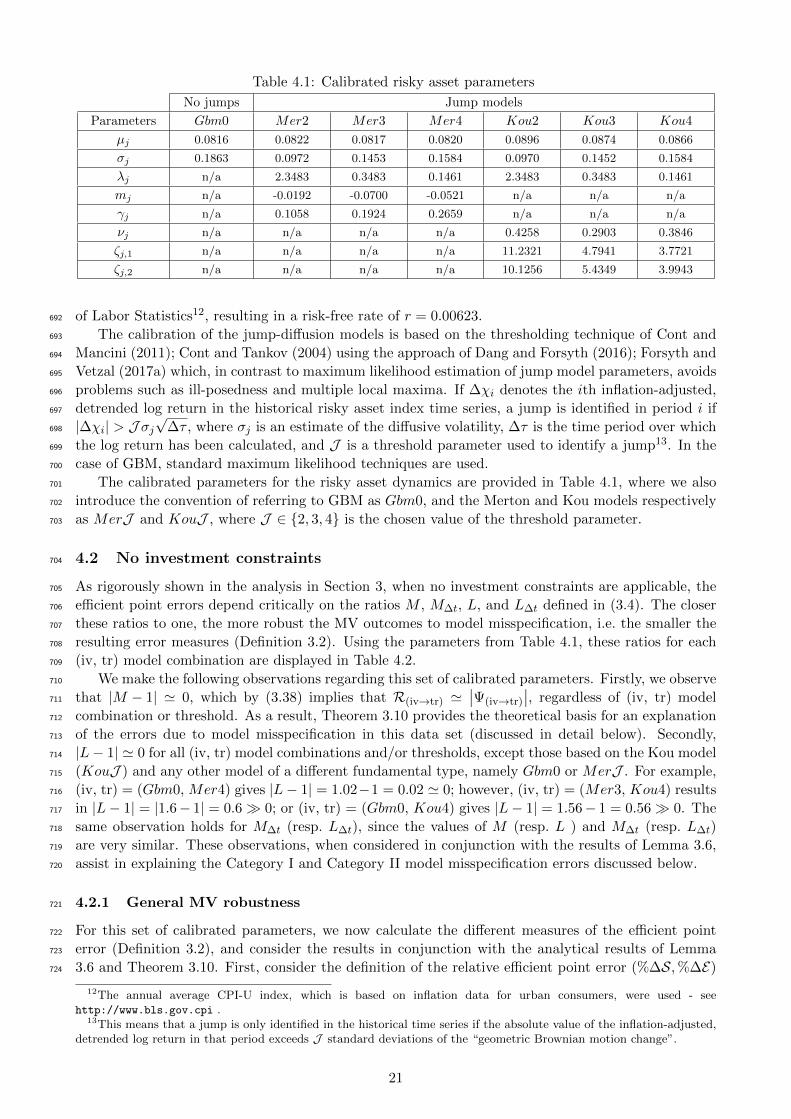
Table 4.1: Calibrated risky asset parameters
No jumps Jump models
Parameters Gbm0 Mer2 Mer3 Mer4 Kou2 Kou3 Kou4
µj 0.0816 0.0822 0.0817 0.0820 0.0896 0.0874 0.0866
σj 0.1863 0.0972 0.1453 0.1584 0.0970 0.1452 0.1584
λj n/a 2.3483 0.3483 0.1461 2.3483 0.3483 0.1461
mj n/a -0.0192 -0.0700 -0.0521 n/a n/a n/a
γj n/a 0.1058 0.1924 0.2659 n/a n/a n/a
νj n/a n/a n/a n/a 0.4258 0.2903 0.3846
ζj,1 n/a n/a n/a n/a 11.2321 4.7941 3.7721
ζj,2 n/a n/a n/a n/a 10.1256 5.4349 3.9943
of Labor Statistics12, resulting in a risk-free rate of r = 0.00623.692
The calibration of the jump-diffusion models is based on the thresholding technique of Cont and693
Mancini (2011); Cont and Tankov (2004) using the approach of Dang and Forsyth (2016); Forsyth and694
Vetzal (2017a) which, in contrast to maximum likelihood estimation of jump model parameters, avoids695
problems such as ill-posedness and multiple local maxima. If ∆χi denotes the ith inflation-adjusted,696
detrended log return in the historical risky asset index time series, a jump is identified in period i if697
|∆χi| > J σj√
∆τ , where σj is an estimate of the diffusive volatility, ∆τ is the time period over which698
the log return has been calculated, and J is a threshold parameter used to identify a jump13. In the699
case of GBM, standard maximum likelihood techniques are used.700
The calibrated parameters for the risky asset dynamics are provided in Table 4.1, where we also701
introduce the convention of referring to GBM as Gbm0, and the Merton and Kou models respectively702
as MerJ and KouJ , where J ∈ 2, 3, 4 is the chosen value of the threshold parameter.703
4.2 No investment constraints704
As rigorously shown in the analysis in Section 3, when no investment constraints are applicable, the705
efficient point errors depend critically on the ratios M , M∆t, L, and L∆t defined in (3.4). The closer706
these ratios to one, the more robust the MV outcomes to model misspecification, i.e. the smaller the707
resulting error measures (Definition 3.2). Using the parameters from Table 4.1, these ratios for each708
(iv, tr) model combination are displayed in Table 4.2.709
We make the following observations regarding this set of calibrated parameters. Firstly, we observe710
that |M − 1| ' 0, which by (3.38) implies that R(iv→tr) '∣∣Ψ(iv→tr)
∣∣, regardless of (iv, tr) model711
combination or threshold. As a result, Theorem 3.10 provides the theoretical basis for an explanation712
of the errors due to model misspecification in this data set (discussed in detail below). Secondly,713
|L− 1| ' 0 for all (iv, tr) model combinations and/or thresholds, except those based on the Kou model714
(KouJ ) and any other model of a different fundamental type, namely Gbm0 or MerJ . For example,715
(iv, tr) = (Gbm0, Mer4) gives |L− 1| = 1.02−1 = 0.02 ' 0; however, (iv, tr) = (Mer3, Kou4) results716
in |L− 1| = |1.6− 1| = 0.6 0; or (iv, tr) = (Gbm0, Kou4) gives |L− 1| = 1.56− 1 = 0.56 0. The717
same observation holds for M∆t (resp. L∆t), since the values of M (resp. L ) and M∆t (resp. L∆t)718
are very similar. These observations, when considered in conjunction with the results of Lemma 3.6,719
assist in explaining the Category I and Category II model misspecification errors discussed below.720
4.2.1 General MV robustness721
For this set of calibrated parameters, we now calculate the different measures of the efficient point722
error (Definition 3.2), and consider the results in conjunction with the analytical results of Lemma723
3.6 and Theorem 3.10. First, consider the definition of the relative efficient point error (%∆S,%∆E)724
12The annual average CPI-U index, which is based on inflation data for urban consumers, were used - seehttp://www.bls.gov.cpi .
13This means that a jump is only identified in the historical time series if the absolute value of the inflation-adjusted,detrended log return in that period exceeds J standard deviations of the “geometric Brownian motion change”.
21

Table 4.2: Key ratios M,M∆t, L and L∆t as per (3.4) for each combination of (iv, tr) model, ∆t = 1.
True
modelRatios
Investor model
Gbm0 Mer2 Mer3 Mer4 Kou2 Kou3 Kou4
Gbm0M , M∆t 1.00 , 1.00 0.99 , 0.99 1.00 , 1.00 0.99 , 0.99 0.90 , 0.90 0.93 , 0.93 0.94 , 0.94
L , L∆t 1.00 , 1.00 0.97 , 0.97 1.03 , 1.03 0.98 , 0.98 0.69 , 0.67 0.69 , 0.67 0.64 , 0.63
Mer2M , M∆t 1.01 , 1.01 1.00 , 1.00 1.01 , 1.01 1.00 , 1.00 0.91 , 0.91 0.94 , 0.93 0.95 , 0.94
L , L∆t 1.03 , 1.03 1.00 , 1.00 1.05 , 1.05 1.00 , 1.00 0.70 , 0.69 0.71 , 0.69 0.66 , 0.65
Mer3M , M∆t 1.00 , 1.00 0.99 , 0.99 1.00 , 1.00 1.00 , 1.00 0.91 , 0.90 0.93 , 0.93 0.94 , 0.94
L , L∆t 0.97 , 0.97 0.95 , 0.95 1.00 , 1.00 0.95 , 0.95 0.67 , 0.65 0.67 , 0.66 0.63 , 0.61
Mer4M , M∆t 1.01 , 1.01 1.00 , 1.00 1.00 , 1.00 1.00 , 1.00 0.91 , 0.91 0.93 , 0.93 0.94 , 0.94
L , L∆t 1.02 , 1.02 1.00 , 1.00 1.05 , 1.05 1.00 , 1.00 0.70 , 0.69 0.70 , 0.69 0.66 , 0.65
Kou2M , M∆t 1.11 , 1.11 1.10 , 1.10 1.10 , 1.11 1.10 , 1.10 1.00 , 1.00 1.03 , 1.03 1.04 , 1.04
L , L∆t 1.46 , 1.49 1.42 , 1.45 1.49 , 1.53 1.43 , 1.46 1.00 , 1.00 1.00 , 1.01 0.94 , 0.94
Kou3M , M∆t 1.08 , 1.08 1.07 , 1.07 1.08 , 1.08 1.07 , 1.07 0.97 , 0.97 1.00 , 1.00 1.01 , 1.01
L , L∆t 1.45 , 1.48 1.42 , 1.44 1.49 , 1.52 1.42 , 1.45 1.00 , 0.99 1.00 , 1.00 0.94 , 0.94
Kou4M , M∆t 1.07 , 1.07 1.06 , 1.06 1.06 , 1.07 1.06 , 1.06 0.96 , 0.96 0.99 , 0.99 1.00 , 1.00
L , L∆t 1.56 , 1.59 1.52 , 1.54 1.60 , 1.63 1.52 , 1.55 1.07 , 1.06 1.07 , 1.07 1.00 , 1.00
defined in (3.2). As shown in Lemma 3.6, given fixed investor model and investment parameters, %∆E725
depends on M or M∆t. Since |M − 1| ' 0 and |M∆t − 1| ' 0, %∆E is fairly negligible for all (iv, tr)726
model combinations. On the other hand, %∆S depends on both (M,L) or both (M∆t, L∆t). Table727
4.2 shows that for (iv, tr) model combinations based on either Gbm0 or MerJ and KouJ , we have728
|L− 1| 0 and |L∆t − 1| 0. It is therefore expected that for these (iv, tr) model combinations,729
%∆S will be large (MV results less robust to model misspecification), while it is negligible for the730
rest of the (iv, tr) model combinations (more robust MV results). That is, %∆S, not %∆E , is the731
key factor in determining the robustness of the MV optimization results for this data set as measured732
by (%∆S,%∆E). Second, considering the error norm (3.3), these observations imply that we would733
indeed expect R(iv→tr) '√
(%∆S)2 =∣∣Ψ(iv→tr)
∣∣ for this data set, which highlights the relevance of734
Theorem 3.10 in explaining the results.735
To further illustrate this point, Table 4.3 shows (%∆S,%∆E) for the (iv, tr) model combinations736
when the true (tr) model is Mer3 and Kou3, for both discrete and continuous rebalancing. Table 4.4737
shows the corresponding results for R(iv→tr) for the same data set.738
Table 4.3: (%∆S,%∆E), defined in (3.2). T = 20, ∆t = 1, Siv = 400, w0 = 100.
True
model
Objec-
tive
Investor model
Gbm0 Mer2 Mer3 Mer4 Kou2 Kou3 Kou4
Mer3
PCMV (-5% , 0%) (-6% , 0%) (0% , 0%) (-6% , 0%) (-22%,-2%) (-26%,-1%) (-32%,-1%)
TCMV (-1% , 0%) (-3% , -1%) (0% , 0%) (-2% , 0%) (-18%,-8%) (-18%,-6%) (-21%,-5%)
PCMV∆t (-4% , 0%) (-5% , 0%) (0% , 0%) (-5% , 0%) (-21%,-3%) (-25%,-2%) (-30%,-2%)
TCMV∆t (-1% , 0%) (-3% , -1%) (0% , 0%) (-2% , 0%) (-19%,-8%) (-19%,-6%) (-22%,-5%)
Kou3
PCMV (66% , 1%) (60% , 1%) (80% , 1%) (60% , 1%) (7% , 0%) (0% , 0%) (-10%, 0%)
TCMV (21% , 7%) (19% , 6%) (22% , 7%) (19% , 6%) (0% , -2%) (0% , 0%) (-3% , 1%)
PCMV∆t (55% , 1%) (50% , 1%) (65% , 1%) (50% , 1%) (5% , -1%) (0% , 0%) (-9% , 0%)
TCMV∆t (22% , 7%) (20% , 6%) (23% , 7%) (20% , 6%) (0% , -2%) (0% , 0%) (-3% , 1%)
739
740
Based on the preceding analysis, in particular Tables 4.2, 4.3 and 4.4, we reach the following conclusions741
on the robustness of MV results for this data set.742
MV optimization can be surprisingly robust to Category I errors, where the investor makes an743
incorrect assumption regarding the fundamental model type, since the resulting efficient point744
22
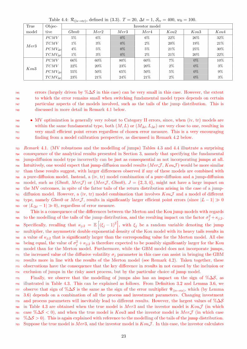
Table 4.4: R(iv→tr), defined in (3.3). T = 20, ∆t = 1, Siv = 400, w0 = 100.
True
model
Objec-
tive
Investor model
Gbm0 Mer2 Mer3 Mer4 Kou2 Kou3 Kou4
Mer3
PCMV 5% 6% 0% 6% 22% 26% 32%
TCMV 1% 3% 0% 2% 20% 19% 21%
PCMV∆t 4% 5% 0% 5% 21% 25% 30%
TCMV∆t 1% 3% 0% 2% 21% 20% 22%
Kou3
PCMV 66% 60% 80% 60% 7% 0% 10%
TCMV 22% 20% 23% 20% 2% 0% 3%
PCMV∆t 55% 50% 65% 50% 5% 0% 9%
TCMV∆t 23% 21% 24% 21% 2% 0% 3%
errors (largely driven by %∆S in this case) can be very small in this case. However, the extent745
to which the error remains small when switching fundamental model types depends on certain746
particular aspects of the models involved, such as the tails of the jump distribution. This is747
discussed in more detail in Remark 4.1 below.748
MV optimization is generally very robust to Category II errors, since, when (iv, tr) models are749
within the same fundamental type, both (M,L) or (M∆t, L∆t) are very close to one, resulting in750
very small efficient point errors regardless of chosen error measure. This is a very encouraging751
finding from a model calibration perspective, as discussed in Remark 4.2 below.752
Remark 4.1. (MV robustness and the modelling of jumps) Tables 4.3 and 4.4 illustrate a surprising753
consequence of the analytical results presented in Section 3, namely that specifying the fundamental754
jump-diffusion model type incorrectly can be just as consequential as not incorporating jumps at all.755
Intuitively, one would expect that jump-diffusion model results (MerJ , KouJ ) would be more similar756
than these results suggest, with larger differences observed if any of these models are combined with757
a pure-diffusion model. Instead, a (iv, tr) model combination of a pure-diffusion and a jump-diffusion758
model, such as (Gbm0, MerJ ) or (MerJ , Gbm0), J = 2, 3, 4, might not have a large impact on759
the MV outcomes, in spite of the fatter tails of the return distribution arising in the case of a jump-760
diffusion model. However, a (iv, tr) model combination that involves KouJ and a model of different761
type, namely Gbm0 or MerJ , results in significantly larger efficient point errors (since |L− 1| 0762
or |L∆t − 1| 0), regardless of error measure.763
This is a consequence of the differences between the Merton and the Kou jump models with regards764
to the modelling of the tails of the jump distribution, and the resulting impact on the factor σ2j +κj,2.765
Specifically, recalling that κj,2 = E[(ξj − 1)2
], with ξj be a random variable denoting the jump766
multiplier, the asymmetric double exponential density of the Kou model with its heavy tails results in767
a value of κj,2 that is significantly larger than the corresponding value for the Merton model. All else768
being equal, the value of σ2j + κj,2 is therefore expected to be possibly significantly larger for the Kou769
model than for the Merton model. Furthermore, while the GBM model does not incorporate jumps,770
the increased value of the diffusive volatility σj parameter in this case can assist in bringing the GBM771
results more in line with the results of the Merton model (see Remark 4.2). Taken together, these772
observations have the consequence that the key difference in results in not caused by the inclusion or773
exclusion of jumps in the risky asset process, but by the particular choice of jump model.774
Finally, we observe that the modelling of jumps also has an impact on the sign of %∆S, as775
illustrated in Table 4.3. This can be explained as follows. From Definition 3.2 and Lemma 3.6, we776
observe that sign of %∆S is the same as the sign of the error multiplier Ψ(iv→tr), which (by Lemma777
3.6) depends on a combination of all the process and investment parameters. Changing investment778
and process parameters will inevitably lead to different results. However, the largest values of %∆S779
in Table 4.3 are obtained when the true model is Mer3 and the investor model is KouJ (in which780
case %∆S < 0), and when the true model is Kou3 and the investor model is MerJ (in which case781
%∆S > 0). This is again explained with reference to the modelling of the tails of the jump distribution.782
Suppose the true model is Mer3, and the investor model is KouJ . In this case, the investor calculates783
23

a standard deviation of terminal wealth Siv consistent with the implications of the heavy tails of the784
asymmetric double exponential distribution, while the true standard deviation S(iv→tr) obtained under785
the (true) Merton model is much lower. This results in S(iv→tr) < Siv, so that %∆S < 0. The case of786
%∆S > 0 can be explained using similar observations.787
Closely related to this discussion, Remark 4.2 below provides a discussion of the implications of788
the MV robustness results for model calibration.789
Remark 4.2. (Implications for model calibration) The MV robustness results have some interesting790
implications for the thresholding calibration methodology used to calibrate the risky asset parameters.791
Assume that the chosen investor model type matches the true model fundamental type but with poten-792
tially different sets of parameters, for example (iv, tr) = (Mer3, Mer2), or (iv, tr) = (Mer3, Mer4).793
The results of Table 4.2 show that the thresholding calibration methodology outlined in Subsection794
4.1 is expected to give very robust MV results regardless of the jump threshold J . Specifically, using795
the analytical results derived in Section 3, the impact of the jump threshold J on the key ratios (3.4)796
is relatively straightforward. In particular, since only the combination of parameters σ2j + λjκj,2 play797
a role in the ratio L, increasing the jump threshold J increases the diffusive volatility σj (more asset798
price moves are due to the diffusion component) and also increases the variance of the jump distri-799
bution and therefore κj,2 (the jumps that occur are larger, regardless of direction), but at the same800
time fewer jumps occur implying a smaller value of λj occur. This robustness of MV results to the801
choice of jump threshold is encouraging since the threshold can also have somewhat counterintuitive802
consequences. For example, Tables 4.3 and 4.4 show that if the true model is Mer2, then an investor803
model of Mer3 would result in M and L values indicative of larger (though still comparatively im-804
material) efficient point errors than if the investor model Mer4 was chosen, which is due precisely to805
the above-mentioned interplay between σj , λj and κj,2 in the thresholding calibration methodology.806
4.2.2 PCMV and TCMV807
Comparing the efficient point errors in this data set for PCMV and TCMV when no investment808
constraints are applicable, the analytical results in Section 3 can be used in conjunction with Tables809
4.2, 4.3 and 4.4 to reach the following conclusions.810
PCMV is less robust to model misspecification than TCMV, regardless of rebalancing frequency811
or underlying models. This is clear from the results for R(iv→tr) reported in Table 4.4, and is812
indeed expected based on the result of Theorem 3.10, since in this data set we observe |M − 1| ' 0813
and |M∆t − 1| ' 0 (see Table 4.2).814
The differences between PCMV and TCMV efficient point errors increases further when the815
(iv,tr) models are of different fundamental types, especially when one model is based on the Kou816
jump-diffusion model formulation. In this particular case, the observation that |L− 1| 0 or817
|L∆t − 1| 0, together with the results of Lemma 3.6 and Theorem 3.10 show that these results818
are expected for this data set.819
Considering the impact of rebalancing frequency on the efficient point error, we observe that820
for TCMV, discrete rebalancing increases the value of R(iv→tr) compared to the corresponding821
values for continuous rebalancing, which is to be expected given the results of Theorem 3.10 (see822
(3.37)). However, the overall impact of rebalancing frequency on the error norm in the case of823
TCMV is actually fairly negligible. In contrast, for PCMV, discrete rebalancing decreases the824
value of R(iv→tr) compared to the corresponding values for continuous rebalancing.825
As noted in the discussion following Theorem 3.10, a simple result comparable to (3.37) cannot be826
given in the case of PCMV, so for analytical purposes these results can be explained rigorously by827
Lemma 3.6 for this particular set of investment and model parameters. However, a more intuitive828
explanation as to why the PCMV and TCMV efficient point errors react so differently to changes829
in rebalancing frequency is particularly useful when no analytical solutions are available, such830
as in the case of the results in Subsection 4.3 below.831
24
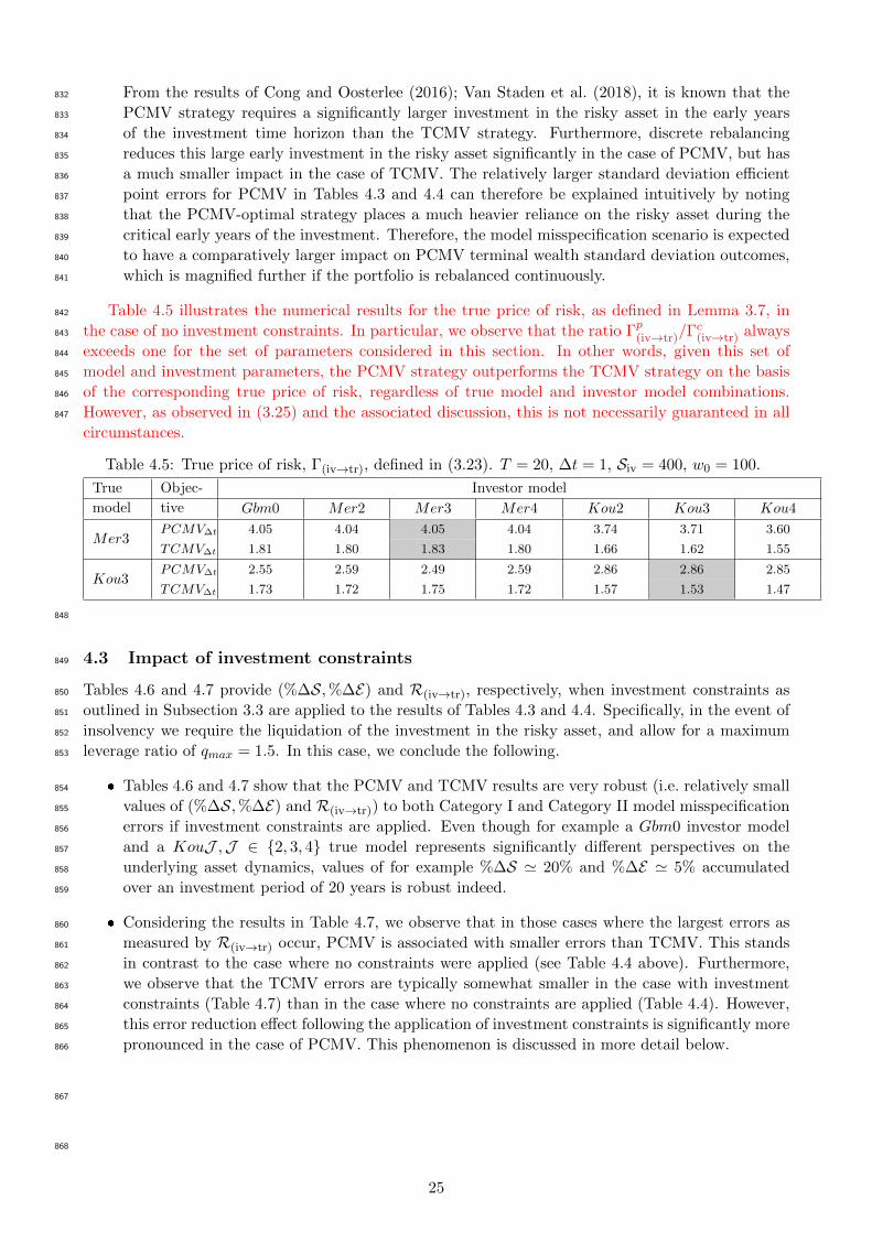
From the results of Cong and Oosterlee (2016); Van Staden et al. (2018), it is known that the832
PCMV strategy requires a significantly larger investment in the risky asset in the early years833
of the investment time horizon than the TCMV strategy. Furthermore, discrete rebalancing834
reduces this large early investment in the risky asset significantly in the case of PCMV, but has835
a much smaller impact in the case of TCMV. The relatively larger standard deviation efficient836
point errors for PCMV in Tables 4.3 and 4.4 can therefore be explained intuitively by noting837
that the PCMV-optimal strategy places a much heavier reliance on the risky asset during the838
critical early years of the investment. Therefore, the model misspecification scenario is expected839
to have a comparatively larger impact on PCMV terminal wealth standard deviation outcomes,840
which is magnified further if the portfolio is rebalanced continuously.841
Table 4.5 illustrates the numerical results for the true price of risk, as defined in Lemma 3.7, in842
the case of no investment constraints. In particular, we observe that the ratio Γp(iv→tr)/Γc(iv→tr) always843
exceeds one for the set of parameters considered in this section. In other words, given this set of844
model and investment parameters, the PCMV strategy outperforms the TCMV strategy on the basis845
of the corresponding true price of risk, regardless of true model and investor model combinations.846
However, as observed in (3.25) and the associated discussion, this is not necessarily guaranteed in all847
circumstances.
Table 4.5: True price of risk, Γ(iv→tr), defined in (3.23). T = 20, ∆t = 1, Siv = 400, w0 = 100.
True
model
Objec-
tive
Investor model
Gbm0 Mer2 Mer3 Mer4 Kou2 Kou3 Kou4
Mer3PCMV∆t 4.05 4.04 4.05 4.04 3.74 3.71 3.60
TCMV∆t 1.81 1.80 1.83 1.80 1.66 1.62 1.55
Kou3PCMV∆t 2.55 2.59 2.49 2.59 2.86 2.86 2.85
TCMV∆t 1.73 1.72 1.75 1.72 1.57 1.53 1.47
848
4.3 Impact of investment constraints849
Tables 4.6 and 4.7 provide (%∆S,%∆E) and R(iv→tr), respectively, when investment constraints as850
outlined in Subsection 3.3 are applied to the results of Tables 4.3 and 4.4. Specifically, in the event of851
insolvency we require the liquidation of the investment in the risky asset, and allow for a maximum852
leverage ratio of qmax = 1.5. In this case, we conclude the following.853
Tables 4.6 and 4.7 show that the PCMV and TCMV results are very robust (i.e. relatively small854
values of (%∆S,%∆E) and R(iv→tr)) to both Category I and Category II model misspecification855
errors if investment constraints are applied. Even though for example a Gbm0 investor model856
and a KouJ ,J ∈ 2, 3, 4 true model represents significantly different perspectives on the857
underlying asset dynamics, values of for example %∆S ' 20% and %∆E ' 5% accumulated858
over an investment period of 20 years is robust indeed.859
Considering the results in Table 4.7, we observe that in those cases where the largest errors as860
measured by R(iv→tr) occur, PCMV is associated with smaller errors than TCMV. This stands861
in contrast to the case where no constraints were applied (see Table 4.4 above). Furthermore,862
we observe that the TCMV errors are typically somewhat smaller in the case with investment863
constraints (Table 4.7) than in the case where no constraints are applied (Table 4.4). However,864
this error reduction effect following the application of investment constraints is significantly more865
pronounced in the case of PCMV. This phenomenon is discussed in more detail below.866
867
868
25
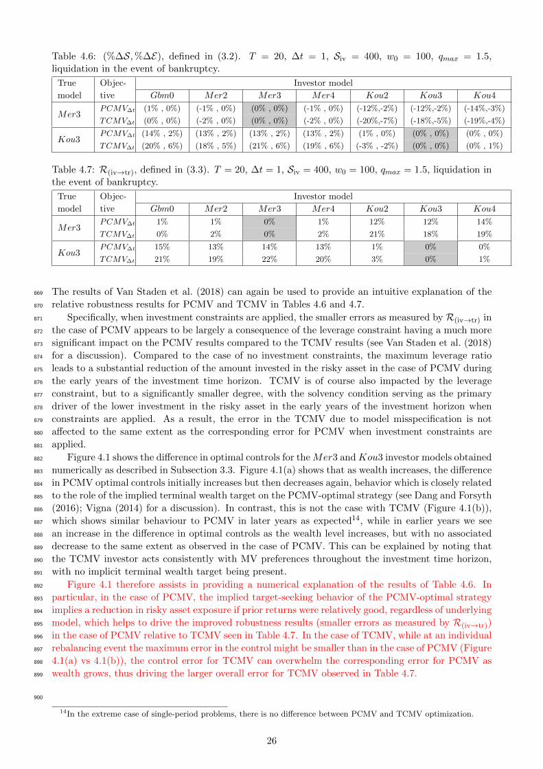
Table 4.6: (%∆S,%∆E), defined in (3.2). T = 20, ∆t = 1, Siv = 400, w0 = 100, qmax = 1.5,liquidation in the event of bankruptcy.
True
model
Objec-
tive
Investor model
Gbm0 Mer2 Mer3 Mer4 Kou2 Kou3 Kou4
Mer3PCMV∆t (1% , 0%) (-1% , 0%) (0% , 0%) (-1% , 0%) (-12%,-2%) (-12%,-2%) (-14%,-3%)
TCMV∆t (0% , 0%) (-2% , 0%) (0% , 0%) (-2% , 0%) (-20%,-7%) (-18%,-5%) (-19%,-4%)
Kou3PCMV∆t (14% , 2%) (13% , 2%) (13% , 2%) (13% , 2%) (1% , 0%) (0% , 0%) (0% , 0%)
TCMV∆t (20% , 6%) (18% , 5%) (21% , 6%) (19% , 6%) (-3% , -2%) (0% , 0%) (0% , 1%)
Table 4.7: R(iv→tr), defined in (3.3). T = 20, ∆t = 1, Siv = 400, w0 = 100, qmax = 1.5, liquidation inthe event of bankruptcy.
True
model
Objec-
tive
Investor model
Gbm0 Mer2 Mer3 Mer4 Kou2 Kou3 Kou4
Mer3PCMV∆t 1% 1% 0% 1% 12% 12% 14%
TCMV∆t 0% 2% 0% 2% 21% 18% 19%
Kou3PCMV∆t 15% 13% 14% 13% 1% 0% 0%
TCMV∆t 21% 19% 22% 20% 3% 0% 1%
The results of Van Staden et al. (2018) can again be used to provide an intuitive explanation of the869
relative robustness results for PCMV and TCMV in Tables 4.6 and 4.7.870
Specifically, when investment constraints are applied, the smaller errors as measured by R(iv→tr) in871
the case of PCMV appears to be largely a consequence of the leverage constraint having a much more872
significant impact on the PCMV results compared to the TCMV results (see Van Staden et al. (2018)873
for a discussion). Compared to the case of no investment constraints, the maximum leverage ratio874
leads to a substantial reduction of the amount invested in the risky asset in the case of PCMV during875
the early years of the investment time horizon. TCMV is of course also impacted by the leverage876
constraint, but to a significantly smaller degree, with the solvency condition serving as the primary877
driver of the lower investment in the risky asset in the early years of the investment horizon when878
constraints are applied. As a result, the error in the TCMV due to model misspecification is not879
affected to the same extent as the corresponding error for PCMV when investment constraints are880
applied.881
Figure 4.1 shows the difference in optimal controls for theMer3 andKou3 investor models obtained882
numerically as described in Subsection 3.3. Figure 4.1(a) shows that as wealth increases, the difference883
in PCMV optimal controls initially increases but then decreases again, behavior which is closely related884
to the role of the implied terminal wealth target on the PCMV-optimal strategy (see Dang and Forsyth885
(2016); Vigna (2014) for a discussion). In contrast, this is not the case with TCMV (Figure 4.1(b)),886
which shows similar behaviour to PCMV in later years as expected14, while in earlier years we see887
an increase in the difference in optimal controls as the wealth level increases, but with no associated888
decrease to the same extent as observed in the case of PCMV. This can be explained by noting that889
the TCMV investor acts consistently with MV preferences throughout the investment time horizon,890
with no implicit terminal wealth target being present.891
Figure 4.1 therefore assists in providing a numerical explanation of the results of Table 4.6. In892
particular, in the case of PCMV, the implied target-seeking behavior of the PCMV-optimal strategy893
implies a reduction in risky asset exposure if prior returns were relatively good, regardless of underlying894
model, which helps to drive the improved robustness results (smaller errors as measured by R(iv→tr))895
in the case of PCMV relative to TCMV seen in Table 4.7. In the case of TCMV, while at an individual896
rebalancing event the maximum error in the control might be smaller than in the case of PCMV (Figure897
4.1(a) vs 4.1(b)), the control error for TCMV can overwhelm the corresponding error for PCMV as898
wealth grows, thus driving the larger overall error for TCMV observed in Table 4.7.899
900
14In the extreme case of single-period problems, there is no difference between PCMV and TCMV optimization.
26
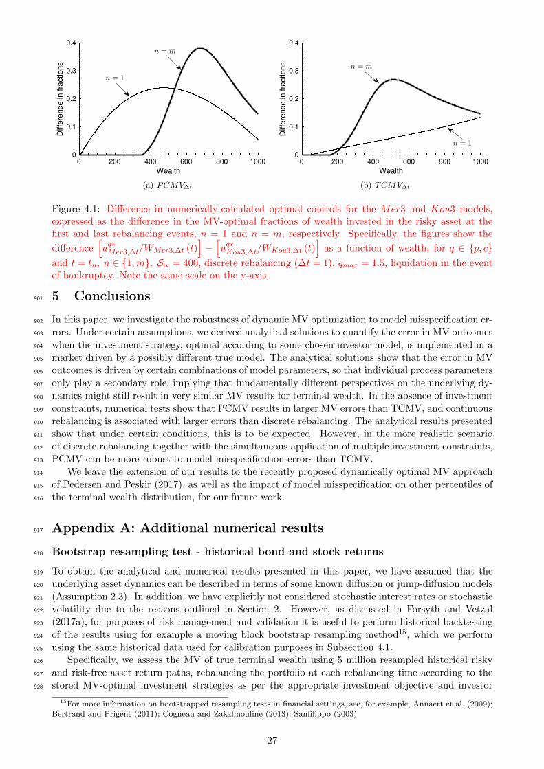
0 200 400 600 800 1000
Wealth
0
0.1
0.2
0.3
0.4
Diffe
ren
ce
in
fra
ctio
ns
n = m
n = 1
(a) PCMV∆t
0 200 400 600 800 1000
Wealth
0
0.1
0.2
0.3
0.4
Diffe
ren
ce
in
fra
ctio
ns
n = m
n = 1
(b) TCMV∆t
Figure 4.1: Difference in numerically-calculated optimal controls for the Mer3 and Kou3 models,expressed as the difference in the MV-optimal fractions of wealth invested in the risky asset at thefirst and last rebalancing events, n = 1 and n = m, respectively. Specifically, the figures show the
difference[uq∗Mer3,∆t/WMer3,∆t (t)
]−[uq∗Kou3,∆t/WKou3,∆t (t)
]as a function of wealth, for q ∈ p, c
and t = tn, n ∈ 1,m. Siv = 400, discrete rebalancing (∆t = 1), qmax = 1.5, liquidation in the eventof bankruptcy. Note the same scale on the y-axis.
5 Conclusions901
In this paper, we investigate the robustness of dynamic MV optimization to model misspecification er-902
rors. Under certain assumptions, we derived analytical solutions to quantify the error in MV outcomes903
when the investment strategy, optimal according to some chosen investor model, is implemented in a904
market driven by a possibly different true model. The analytical solutions show that the error in MV905
outcomes is driven by certain combinations of model parameters, so that individual process parameters906
only play a secondary role, implying that fundamentally different perspectives on the underlying dy-907
namics might still result in very similar MV results for terminal wealth. In the absence of investment908
constraints, numerical tests show that PCMV results in larger MV errors than TCMV, and continuous909
rebalancing is associated with larger errors than discrete rebalancing. The analytical results presented910
show that under certain conditions, this is to be expected. However, in the more realistic scenario911
of discrete rebalancing together with the simultaneous application of multiple investment constraints,912
PCMV can be more robust to model misspecification errors than TCMV.913
We leave the extension of our results to the recently proposed dynamically optimal MV approach914
of Pedersen and Peskir (2017), as well as the impact of model misspecification on other percentiles of915
the terminal wealth distribution, for our future work.916
Appendix A: Additional numerical results917
Bootstrap resampling test - historical bond and stock returns918
To obtain the analytical and numerical results presented in this paper, we have assumed that the919
underlying asset dynamics can be described in terms of some known diffusion or jump-diffusion models920
(Assumption 2.3). In addition, we have explicitly not considered stochastic interest rates or stochastic921
volatility due to the reasons outlined in Section 2. However, as discussed in Forsyth and Vetzal922
(2017a), for purposes of risk management and validation it is useful to perform historical backtesting923
of the results using for example a moving block bootstrap resampling method15, which we perform924
using the same historical data used for calibration purposes in Subsection 4.1.925
Specifically, we assess the MV of true terminal wealth using 5 million resampled historical risky926
and risk-free asset return paths, rebalancing the portfolio at each rebalancing time according to the927
stored MV-optimal investment strategies as per the appropriate investment objective and investor928
15For more information on bootstrapped resampling tests in financial settings, see, for example, Annaert et al. (2009);Bertrand and Prigent (2011); Cogneau and Zakalmouline (2013); Sanfilippo (2003)
27
model. The resampled paths are constructed by dividing the horizon T into k blocks of size b years929
(i.e. T = kb), where block sizes of b = 5 years and b = 10 years are considered16. Each individual930
resampled path is constructed by selecting k blocks at random (with replacement) from the historical931
data, with each block starting at a random quarter and with blocks being wrapped around to avoid end932
effects in the data, with selected blocks being concatenated to produce the path. In Table A.1, we use933
the resampled historical paths as the “true” model to report the relative efficient point error exactly934
as before. We observe that (i) the relative efficient point error is of similar order of magnitude using935
resampled historical data as in the case of using a model (Table 4.6), and (ii) the qualitative conclusions936
regarding the relative robustness of PCMV vs. TCMV optimization for the models considered in Table937
4.6 appear to hold.938
More generally, the results of Table A.1 validate our overall conclusions regarding the robustness of939
MV optimization to model misspecification errors, as well as Assumption 2.2 regarding interest rates.940
We leave a detailed discussion of the different performance of PCMV and TCMV-optimal controls in941
the case of resampled historical data for our future work.
Table A.1: (%∆S,%∆E) calculated using numerical results based on resampled historical data. T =20, ∆t = 1, Siv = 400, w0 = 100, qmax = 1.5, liquidation in the event of bankruptcy.
Block
size
Objec-
tive
Investor model
Gbm0 Mer2 Mer3 Mer4 Kou2 Kou3 Kou4
5 yearsPCMV∆t (6% , 1%) (5% , 1%) (5% , 1%) (5% , 1%) (-7% , -1%) (-7% , -1%) (-7% , 0%)
TCMV∆t (-2% , 0%) (-4% , -1%) (-2% , 0%) (-3% , -1%) (-11%,-1%) (-10%,-1%) (-10%,-1%)
10
years
PCMV∆t (7% , 3%) (5% , 3%) (6% , 3%) (5% , 2%) (-7% , 1%) (-7% , 1%) (-7% , -1%)
TCMV∆t (-8% , 0%) (-10%,-1%) (-9% , 0%) (-10%,-1%) (-14%, 0%) (-13%,-1%) (-12%, 0%)
942
Other attributes of the terminal wealth distribution943
The preceding results only focused on the mean and variance of terminal wealth. However, depending944
on the application, the investor may also be concerned with other aspects of the terminal wealth945
distribution, especially given the possibility of jumps in the risky asset process. For example, in946
pension fund applications (see, for example, Forsyth and Vetzal (2017a)) the probability that the947
terminal wealth Wtr,∆t (T ) falls below some minimum level (for illustrative purposes assumed here to948
be w0erT ) may be of interest. Other risk metrics such as the Value-at-Risk (VaR) or Conditional Value-949
at-Risk (CVaR) might also be considered important - see Rockafellar and Uryasev (2002). Table A.2950
uses the Monte Carlo simulations described above to estimate the probability P[Wtr,∆t (T ) ≤ w0e
rT],951
as well as the 95%-VaR and 95%-CVaR17.952
In this case, concluding that MV optimization is robust to model misspecification errors depends953
not only on some (percentile-based) definition of robustness, but also on the associated implications954
of estimating some critical value incorrectly. As a result, we leave the broader implications of model955
misspecification for the terminal wealth distribution for our future work.956
References957
Annaert, J., S. Osslaer, and B. Verstraete (2009). Performance evaluation of portfolio insurance strategies using958
stochastic dominance criteria. Journal of Banking and Finance (33), 272–280.959
Bailey, D. and M. Lopez de Prado (2012). Balanced baskets: A new approach to trading and hedging risks.960
Journal of Investment Strategies 1(4), 21–62.961
16Blocks of historical data of sufficiently large size is required to capture the serial dependence possibly present in thedata (see Cogneau and Zakalmouline (2013)), but block sizes that are too large result in unreliable variance estimates.We therefore follow Forsyth and Vetzal (2017a) in considering multiple block sizes.
17The α-VaR (resp. α-CVaR) is the VaR (resp. CVaR) corresponding to a confidence level α. In our application,this means that 5% of the simulated values of Wtr,∆t (T ) are equal to or below the reported 95%-VaR value, while thereported 95%-CVaR value is the mean of the simulated values of Wtr,∆t (T ) equal to or less than the 95%-VaR - seeMiller and Yang (2017); Rockafellar and Uryasev (2002) for a discussion.
28

Table A.2: Three quantities associated with the simulated true terminal wealth Wtr,∆t (T ) distribution,discrete rebalancing: P
[Wtr,∆t (T ) ≤ w0e
rT]
(“Probability”), 95%-VaR and 95%-CVaR. T = 20, ∆t =1, Siv = 400, w0 = 100, qmax = 1.5, liquidation in the event of bankruptcy.
(a) PCMV
True model QuantityInvestor model
Mer3 Kou3
Mer3
Probability 12.9% 12.6%
95% -VaR 52.4 49.0
95%-CVaR 30.3 25.0
Kou3
Probability 17.1% 16.8%
95%-VaR 24.5 16.3
95%-CVaR 5.0 6.2
(b) TCMV
True model QuantityInvestor model
Mer3 Kou3
Mer3
Probability 11.0% 10.5%
95%-VaR 63.4 64.8
95%-CVaR 38.3 36.5
Kou3
Probability 14.1% 13.5%
95%-VaR 40.4 36.2
95%-CVaR 18.1 16.6
Basak, S. and G. Chabakauri (2010). Dynamic mean-variance asset allocation. Review of Financial Studies 23,962
2970–3016.963
Bertrand, P. and J. Prigent (2011). Omega performance measure and portfolio insurance. Journal of Banking964
and Finance (35), 1811–1823.965
Best, M. and R. Grauer (1991). Sensitivity analysis for mean-variance portfolio problems. Management Science966
37(8), 980–989.967
Bjork, T. and A. Murgoci (2014). A theory of Markovian time-inconsistent stochastic control in discrete time.968
Finance and Stochastics (18), 545–592.969
Bjork, T., A. Murgoci, and X. Zhou (2014). Mean-variance portfolio optimization with state-dependent risk970
aversion. Mathematical Finance (1), 1–24.971
Bourgeron, T., E. Lezmi, and T. Roncalli (2018). Robust asset allocation for robo-advisors. Working paper .972
Britten-Jones, M. (1999). The sampling error in estimates of mean-variance efficient portfolio weights. The973
Journal of Finance (2).974
Brodie, J., I. Daubechies, C. De Mol, D. Giannone, and I. Loris (2009). Sparse and stable Markowitz portfolios.975
Proceedings of the National Academy of Sciences 106(30), 12267–12272.976
Bruder, B., N. Gaussel, J.-C. Richard, and T. Roncalli (2013). Regularization of portfolio allocation. Working977
paper .978
Bruder, B., N. Kostyuchyk, and T. Roncalli (2016). Risk parity portfolios with skewness risk: an application979
to factor investing and alternative risk premia. Working paper .980
Carrasco, M. and N. Noumon (2010). Optimal portfolio selection using regularization. Discussion paper,981
University of Montreal .982
Choueifaty, Y. and Y. Coignard (2008). Toward maximum diversification. Journal of Portfolio Management983
35(1), 40–51.984
Cogneau, P. and V. Zakalmouline (2013). Block bootstrap methods and the choice of stocks for the long run.985
Quantitative Finance (13), 1443–1457.986
Cong, F. and C. Oosterlee (2016). On pre-commitment aspects of a time-consistent strategy for a mean-variance987
investor. Journal of Economic Dynamics and Control 70, 178–193.988
Cong, F. and C. Oosterlee (2017). On robust multi-period pre-commitment and time-consistent mean-variance989
portfolio optimization. International Journal of Theoretical and Applied Finance 20(7).990
Cont, R. and C. Mancini (2011). Nonparametric tests for pathwise properties of semi-martingales. Bernoulli991
(17), 781–813.992
Cont, R. and P. Tankov (2004). Financial modelling with jump processes. Chapman and Hall / CRC Press.993
Cui, X., D. Li, S. Wang, and S. Zhu (2012). Better than dynamic mean-variance: Time inconsistency and free994
cash flow stream. Mathematical Finance 22(2), 346–378.995
Dang, D. and P. Forsyth (2014). Continuous time mean-variance optimal portfolio allocation under jump996
diffusion: A numerical impulse control approach. Numerical Methods for Partial Differential Equations 30,997
664–698.998
Dang, D. and P. Forsyth (2016). Better than pre-commitment mean-variance portfolio allocation strategies: A999
semi-self-financing Hamilton–Jacobi–Bellman equation approach. European Journal of Operational Research1000
(250), 827–841.1001
Dang, D., P. Forsyth, and K. Vetzal (2017). The 4 percent strategy revisited: a pre-commitment mean-variance1002
optimal approach to wealth management. Quantitative Finance 17(3), 335–351.1003
29
Dang, D., P. Forsyth, and Y.Li (2016). Convergence of the embedded mean-variance optimal points with discrete1004
sampling. Numerische Mathematik (132), 271–302.1005
De Jong, M. (2018). Portfolio optimization in an uncertain world. Journal of Asset Management 19(4), 216–221.1006
DeMiguel, V., L. Garlappi, F. Nogales, and R. Uppal (2009). A generalized approach to portfolio optimization:1007
Improving performance by constraining portfolio norms. Management Science 55(5), 798–812.1008
Elton, E., M. Gruber, S. Brown, and W. Goetzmann (2014). Modern portfolio theory and investment analysis.1009
Wiley, 9th edition.1010
Forsyth, P. and K. Vetzal (2017a). Dynamic mean variance asset allocation: Tests for robustness. International1011
Journal of Financial Engineering 4:2. 1750021 (electronic).1012
Forsyth, P. and K. Vetzal (2017b). Robust asset allocation for long-term target-based investing. International1013
Journal of Theoretical and Applied Finance 20(3).1014
Garlappi, L., R. Uppal, and T. Wang (2007). Portfolio selection with parameter and model uncertainty: A1015
multi-prior approach. The Review of Financial Studies 20(1).1016
Gulpinar, N. and B. Rustem (2007). Worst-case robust decisions for multi-period mean-variance portfolio1017
optimization. European Journal of Operational Research (183), 981–1000.1018
Kim, J., W. Kim, and F. Fabozzi (2014). Recent developments in robust portfolios with a worst-case approach.1019
Journal of Optimization Theory and Applications (161), 103–121.1020
Kou, S. (2002). A jump-diffusion model for option pricing. Management Science 48(8), 1086–1101.1021
Kuhn, D., P. Parpas, B. Rustem, and R. Fonseca (2009). Dynamic mean-variance portfolio analysis under model1022
risk. Journal of Computational Finance 12(4), 91–115.1023
Lee, W. (2011). Risk-based asset allocation: A new answer to an old question? Journal of Portfolio Management1024
(37), 11–28.1025
Li, D. and W.-L. Ng (2000). Optimal dynamic portfolio selection: multi period mean variance formulation.1026
Mathematical Finance 10, 387–406.1027
Li, D., X. Rong, and H. Zhao (2015a). Time-consistent reinsurance–investment strategy for a mean–variance1028
insurer under stochastic interest rate model and inflation risk. Insurance: Mathematics and Economics 64,1029
28–44.1030
Li, Y. and P. Forsyth (2019). A data-driven neural network approach to optimal asset allocation for target1031
based defined contribution pension plans. Insurance: Mathematics and Economics (86), 189–204.1032
Li, Y., H. Qiao, S. Wang, and L. Zhang (2015b). Time-consistent investment strategy under partial information.1033
Insurance: Mathematics and Economics 65, 187–197.1034
Li, Z., Y. Zeng, and Y. Lai (2012). Optimal time-consistent investment and reinsurance strategies for insurers1035
under Heston’s SV model. Insurance: Mathematics and Economics 51, 191–203.1036
Liang, Z. and M. Song (2015). Time-consistent reinsurance and investment strategies for mean–variance insurer1037
under partial information. Insurance: Mathematics and Economics 65, 66–76.1038
Lin, X. and Y. Qian (2016). Time-consistent mean-variance reinsurance-investment strategy for insurers under1039
cev model. Scandinavian Actuarial Journal (7), 646–671.1040
Lopez de Prado, M. (2016). Building diversified portfolios that outperform out-of-sample. Journal of Portfolio1041
Management 42(4), 59–69.1042
Ma, K. and P. Forsyth (2016). Numerical solution of the Hamilton-Jacobi-Bellman formulation for continuous1043
time mean variance asset allocation under stochastic volatility. Journal of Computational Finance 20:1, 1–37.1044
Maillard, S., T. Roncalli, and J. Teiletche (2010). The properties of equally weighted risk contribution portfolios.1045
Journal of Portfolio Management 36(4), 60–70.1046
Markowitz, H. (1952). Portfolio selection. The Journal of Finance 7(1), 77–91.1047
Merton, R. (1976). Option pricing when underlying stock returns are discontinuous. Journal of Financial1048
Economics 3, 125–144.1049
Michaud, R. and R. Michaud (2008). Efficient asset management: A practical guide to stock portfolio optimiza-1050
tion and asset allocation. Oxford University Press, 2 edition.1051
Miller, C. and I. Yang (2017). Optimal control of conditional value-at-risk in continuous time. SIAM Journal1052
on Control and Optimization 55(2), 856–884.1053
Pedersen, J. and G. Peskir (2017). Optimal mean-variance portfolio selection. Mathematics and Financial1054
Economics (11), 137–160.1055
Perrin, S. and T. Roncalli (2019). Machine learning optimization algorithms and portfolio allocation. Working1056
paper .1057
Qian, E. (2005). Risk parity portfolios: Efficient portfolios through true diversification. Technical report,1058
Panagora Asset Management.1059
Richard, J.-C. and T. Roncalli (2015). Smart beta: managing diversification of minimum variance portfolios.1060
ISTE Press Elsevier.1061
30
Rockafellar, R. and S. Uryasev (2002). Conditional value-at-risk for general loss distributions. Journal of1062
Banking and Finance (26), 1443–1471.1063
Roncalli, T. (2013). Introduction to risk parity and budgeting. Financial Mathematics Series. Chapman and1064
Hall / CRC Press.1065
Roncalli, T. (2015). Introducing expected returns into risk parity portfolios: A new framework for asset1066
allocation. Bankers, Markets and Investors (138), 18–28.1067
Sanfilippo, G. (2003). Stocks, bonds and the investment horizon: a test of time diversification on the french1068
market. Quantitative Finance (3), 345–531.1069
Sato, Y. (2019). Model-free reinforcement learning for financial portfolios: A brief survey. Working paper .1070
Scherer, B. (2007). Portfolio construction and risk budgeting. Risk Books, 3rd edition.1071
Strub, M., D. Li, and X. Cui (2019). An enhanced mean-variance framework for robo-advising applications.1072
SSRN 3302111.1073
Sun, J., Z. Li, and Y. Zeng (2016). Precommitment and equilibrium investment strategies for defined contribu-1074
tion pension plans under a jump–diffusion model. Insurance: Mathematics and Economics (67), 158–172.1075
Tutuncu, R. and M. Koenig (2004). Robust asset allocation. Annals of Operations Research (132), 157–187.1076
Van Staden, P. M., D. Dang, and P. Forsyth (2018). Time-consistent mean-variance portfolio optimization: a1077
numerical impulse control approach. Insurance: Mathematics and Economics (83C), 9–28.1078
Van Staden, P. M., D. Dang, and P. Forsyth (2019). Mean-quadratic variation portfolio optimization: A desirable1079
alternative to time-consistent mean-variance optimization? SIAM Journal on Financial Mathematics 10(3),1080
815–856.1081
Vigna, E. (2014). On efficiency of mean-variance based portfolio selection in defined contribution pension1082
schemes. Quantitative Finance 14(2), 237–258.1083
Vigna, E. (2016). On time consistency for mean-variance portfolio selection. Working paper, Collegio Carlo1084
Alberto (476).1085
Wang, H. and X. Zhou (2019). Continuous-time mean-variance portfolio selection: A reinforcement learning1086
framework. Working paper .1087
Wang, J. and P. Forsyth (2011). Continuous time mean variance asset allocation: A time-consistent strategy.1088
European Journal of Operational Research (209), 184–201.1089
Yu, P. (1971). Cone convexity, cone extreme points, and nondominated solutions in decision problem with1090
multiobjectives. Journal of Optimization Theory and Applications (7), 11–28.1091
Zeng, Y. and Z. Li (2011). Optimal time-consistent investment and reinsurance policies for mean-variance1092
insurers. Insurance: Mathematics and Economics 49(1), 145–154.1093
Zeng, Y., Z. Li, and Y. Lai (2013). Time-consistent investment and reinsurance strategies for mean–variance1094
insurers with jumps. Insurance: Mathematics and Economics 52, 498–507.1095
Zhang, L., Z. Li, Y. Xu, and Y. Li (2016). Multi-period mean variance portfolio selection under incomplete1096
information. Applied Stochastic Models in Business and Industry (32), 753–774.1097
Zhang, M. and P. Chen (2016). Mean-variance asset-liability management under constant elasticity of variance1098
process. Insurance: Mathematics and Economics (70), 11–18.1099
Zhou, X. and D. Li (2000). Continuous time mean variance portfolio selection: a stochastic LQ framework.1100
Applied Mathematics and Optimization 42, 19–33.1101
Zweng, Y. and Z. Li (2011). Asset liability management under benchmark and mean-variance criteria in a jump1102
diffusion market. Journal of Systems Science and Complexity (24), 317–327.1103
31