
The Structural Use of Synthetic Fibres: Thickness Design of ...
156
The Structural Use of Synthetic Fibres: Thickness Design of Concrete Slabs on Grade by Jacques Bothma December 2013 Thesis presented in fulfilment of the requirements for the degree of Masters in the Faculty of Civil Engineering at Stellenbosch University Supervisor: Prof. William Peter Boshoff
Transcript of The Structural Use of Synthetic Fibres: Thickness Design of ...

The Structural Use of Synthetic Fibres:
Thickness Design of Concrete Slabs on Grade
by
Jacques Bothma
December 2013
Thesis presented in fulfilment of the requirements for the degree of
Masters in the Faculty of Civil Engineering at Stellenbosch University
Supervisor: Prof. William Peter Boshoff

i
Declaration
By submitting this thesis/dissertation electronically, I declare that the entirety of the work
contained therein is my own, original work, that I am the sole author thereof (save to the
extent explicitly otherwise stated), that reproduction and publication thereof by Stellenbosch
University will not infringe any third party rights and that I have not previously in its entirety
or in part submitted it for obtaining any qualification.
…………………………………………… Signature
Date: December 2013
Copyright © 2013 University of Stellenbosch
All rights reserved
Stellenbosch University http://scholar.sun.ac.za

ii
Abstract
Concrete is used in most of the modern day infrastructure. It is a building material for which there
exist various design codes and guidelines for its use and construction. It is strong in compression, but
lacks tensile strength in its fresh and hardened states and, when unreinforced, fails in a brittle manner.
The structural use of synthetic fibres in concrete is investigated in this study to determine its effect on
enhancing the mechanical properties of concrete. Slabs on grade are used as the application for which
the concrete is tested. The material behaviour is investigated in parallel with two floor design theories.
These are the Westegaard theory and the Yield-Line theory. The Westegaard theory uses elastic
theory to calculate floor thicknesses while the Yield-Line theory includes plastic behaviour.
Conceptual designs are performed with the two theories and material parameters are determined from
flexural tests conducted on synthetic fibre reinforced concrete (SynFRC) specimens. Large scale slab
tests are performed to verify design values from the two theories.
Higher loads till first-crack were measured during tests with concrete slabs reinforced with
polypropylene fibres than for unreinforced concrete. It is found that the use of synthetic fibres in
concrete increases the post-crack ductility of the material. The Westegaard theory is conservative in
its design approach by over-estimating design thicknesses. This was concluded as unreinforced slabs
reached higher failure loads than predicted by this theory. The Yield-Line theory predicts design
thicknesses more accurately while still accounting for the requirements set by the ultimate- and
serviceability limit states. By using SynFRC in combination with the Yield-Line theory as design
method, thinner floor slabs can be obtained than with the Westegaard theory.
Stellenbosch University http://scholar.sun.ac.za

iii
Opsomming
Beton word gebruik as boumateriaal in meeste hedendaagse infrastruktuur. Daar bestaan verskeie
ontwerp kodes en riglyne vir die gebruik en oprig van beton strukture. Alhoewel beton sterk in
kompressie is, het beton ‘n swak treksterkte in beide die vars- en harde fases en faal dit in ‘n bros
manier indien onbewapen.
Die gebruik van sintetiese vesels in beton word in hierdie projek ondersoek om die invloed daarvan
op die eienskappe van die meganiesegedrag van beton te bepaal. Grond geondersteunde vloere word
as toepassing gebruik. Parallel met die materiaalgedrag wat ondersoek word, word twee ontwerps-
teorieë ook ondersoek. Dit is die teorie van Westegaard en die Swig-Lyn teorie. Die teorie van
Westegaard gebruik elastiese teorie in ontwerpsberekeninge terwyl die Swig-Lyn teorie ‘n plastiese
analise gebruik.
‘n Konseptuele vloerontwerp is gedoen deur beide die ontwerpsmetodes te gebruik.
Materiaalparameters is bepaal deur buig-toetse uit te voer op sintetiesevesel-bewapende beton.
Grootskaalse betonblaaie is gegiet en getoets om die akkuraatheid van die twee metodes te verifieer.
Die betonblaaie wat bewapen was met polipropileen vesels het groter laste gedra tot by faling as die
blaaie wat nie bewapen was nie. Die vesels verbeter die gedrag van beton in die plastiese gebied van
materiaalgedrag deurdat laste ondersteun word nadat die beton alreeds gekraak het. Die Westegaard
teorie kan as konserwatief beskou word deurdat dit vloerdiktes oorskat. Hierdie stelling is gegrond op
eksperimentele data wat bewys dat onbewapende betonblaaie groter laste kan dra as wat voorspel
word deur die Westegaard teorie. Die Swig-Lyn teorie voorspel ontwerpsdiktes meer akkuraat terwyl
daar steeds aan die vereistes van swigting en diensbaarheid voldoen word. Deur gebruik te maak van
sintetiese vesels en die Swig-Lyn teorie kan dunner betonblaaie ontwerp word as met die Westegaard
teorie.
Stellenbosch University http://scholar.sun.ac.za

iv
Acknowledgements
I would like to thank my study leader, Prof. W.P. Boshoff, for all his help and support during the
course of this project. Further would I like to thank my parents, Japie and Carine Bothma, for their
support during my studies. Lastly I would like to thank the laboratory staff and industry partners for
their support with the experimental work.
Stellenbosch University http://scholar.sun.ac.za
v
Table of Contents
Declaration.............................................................................................................i
Abstract.................................................................................................................ii
Opsomming.........................................................................................................iii
Acknowledgements..............................................................................................iv
Table of Contents..................................................................................................v
List of Figures....................................................................................................viii
List of Tables.......................................................................................................xi
Symbols and Abbreviations...............................................................................xiii
Chapter 1. Introduction .................................................................................. 1
Chapter 2. Fibre Reinforced Concrete ............................................................ 3
2.1 Fibre Materials and Types ........................................................................................................ 3
2.2 Mechanical Behaviour of FRC ................................................................................................. 6
2.2.1 Flexural and Shear Strength of FRC ................................................................................ 10
2.2.2 Tensile Strength of FRC .................................................................................................. 12
2.2.3 Compressive Strength of FRC ......................................................................................... 13
2.2.4 Fire Resistance and Durability ......................................................................................... 14
2.2.5 Impact Resistance of FRC ............................................................................................... 15
2.3 Concluding Summary ............................................................................................................ 17
Chapter 3. Design of Slabs on Grade ........................................................... 18
3.1 Subgrades and Subbases ........................................................................................................ 19
3.2 Concrete for Industrial Floors ................................................................................................ 21
3.3 Joints in Floors ...................................................................................................................... 23
Stellenbosch University http://scholar.sun.ac.za

vi
3.4 Typical Loads ........................................................................................................................ 25
3.5 The Westegaard Theory ......................................................................................................... 26
3.5.1 Point Loads ..................................................................................................................... 27
3.5.2 Dynamic Loads ............................................................................................................... 30
3.5.3 Distributed Loads ............................................................................................................ 31
3.6 The Yield-Line Theory .......................................................................................................... 33
3.7 Concluding Summary ............................................................................................................ 38
Chapter 4. Conceptual Slab Design ............................................................. 39
4.1 Thickness Design with Westegaard’s theory........................................................................... 40
4.1.1 Design for Post Loads ..................................................................................................... 41
4.1.2 Design for Wheel Loads (Single-wheel axle load) ........................................................... 44
4.1.3 Distributed Loads ............................................................................................................ 46
4.2 Design with the Yield–Line Theory........................................................................................ 47
4.2.1 Point Loads ..................................................................................................................... 48
4.2.2 Wheel Loads ................................................................................................................... 53
4.2.3 Distributed Loads ............................................................................................................ 53
4.3 Comparing the Results ........................................................................................................... 55
4.4 Concluding Summary ............................................................................................................ 57
Chapter 5. Experimental Tests on Material Parameters ................................ 58
5.1 Mix Design ............................................................................................................................ 58
5.2 Test Setup .............................................................................................................................. 60
5.3 Results ................................................................................................................................... 61
5.3.1 Compressive Strength ..................................................................................................... 61
5.3.2 Flexural Strength ............................................................................................................. 61
5.4 Discussion ............................................................................................................................. 63
5.5 Concluding Summary ............................................................................................................ 64
Chapter 6. Large Scale Slab Tests................................................................ 65
6.1 Mix Design and Shuttering..................................................................................................... 65
Stellenbosch University http://scholar.sun.ac.za

vii
6.2 Mixing- and Pouring Processes .............................................................................................. 66
6.3 Test Setup .............................................................................................................................. 68
6.4 Results of Slab Tests .............................................................................................................. 70
6.4.1 Test Nr.1 (no fibres and large loading area) ..................................................................... 72
6.4.2 Test Nr. 2 (fibres and large loading area) ......................................................................... 74
6.4.3 Test Nr.3 (fibres and small loading area) ......................................................................... 76
6.4.4 Test Nr.4 (no fibres and small loading area) .................................................................... 78
6.5 Discussion on Results of Slab Tests ....................................................................................... 79
6.6 Concluding Summary ............................................................................................................ 81
Chapter 7. Analysis and Discussion of Results ............................................ 82
7.1 Design Using the Westegaard Theory..................................................................................... 83
7.1.1 Design Load for Large Load Plate ................................................................................... 83
7.1.2 Design Load for Small Load Plate ................................................................................... 84
7.2 Design Using the Yield-Line Theory ...................................................................................... 85
7.2.1 Design for the Large Loading Area.................................................................................. 86
7.2.2 Design for the Small Loading Area.................................................................................. 87
7.3 Finite Element Analysis ......................................................................................................... 88
7.4 Comparison with Experimental Tests ..................................................................................... 94
7.5 Concluding Summary ............................................................................................................ 97
Chapter 8. Conclusions and Recommendations ........................................... 98
Chapter 9. References ................................................................................ 100
Addendum A: Design tables and charts for using Westegaard’s theory
Addendum B: Floor thickness design with Westegaard’s theory and the Yield-Line theory.
Addendum C: Checks to confirm the capacity of the slabs designed for Chapter 7 by using the
Westegaard theory.
Stellenbosch University http://scholar.sun.ac.za

viii
List of Figures
Figure 2.1: Steel fibre geometries (Concrete Society UK TR 63, 2007). ............................................. 5
Figure 2.2: Examples of polypropylene micro- and macro fibres. ....................................................... 6
Figure 2.3: Strain hardening and strain softening behaviour of different FRC’s (Brandt, 2008) ........... 8
Figure 2.4: Elastic stress block (left) and a proposed stress block for FRC (Concrete Society UK TR
65, 2007). ........................................................................................................................................ 10
Figure 2.5: Test set setup for panel tests according to EFNARC (Ding & Kurnele, 1999). ................ 11
Figure 2.6: Comparison of SRC to SFRC for different fibre dosages at an age of 48h (Ding &
Kurstele, 1999). ............................................................................................................................... 11
Figure 2.7: Comparison of hybrid fibre reinforcement to HPPFR (Cengiz & Turanli, 2005). ............ 12
Figure 2.8: Comparison between splitting tensile strength of GFRC and PFRC with unreinforced
concrete after Choi and Yuan (2005). .............................................................................................. 13
Figure 2.9: Compressive strength of different concrete mixes comprising of plain and fibre reinforced
concrete (Alhozaimy et al., 1995) .................................................................................................... 14
Figure 2.10: Impact load test setup (Wang et al., 1996). ................................................................... 16
Figure 2.11: Projectile for impact testing (Zhang et al., 2007). ......................................................... 17
Figure 3.1: Hard- and soft spots and its consequences on concrete floors (Marais & Perrie, 1993). ... 21
Figure 3.2: Transfer mechanisms across formed free-movement joint (Concrete Society, UK, 2003).24
Figure 3.3: Sawn restrained-movement joint with the use of steel fabric (Concrete Society UK, 2003).
........................................................................................................................................................ 24
Figure 3.4: Tied or restrained-movement joint (Concrete Society UK, 2003). ................................... 25
Figure 3.5: Critical section under shear loading, where h is the slab depth. ....................................... 28
Figure 3.6: Design chart for post loads and a k-value of 30kPa/mm (Marais & Perrie, 1993). ........... 29
Figure 3.7: Thickness design chart for single-wheel axle trucks (Marais & Perrie, 1993). ................. 32
Figure 3.8: Examples of yield-line patterns for point loads on a concrete floor (Concrete Society,
2003). .............................................................................................................................................. 33
Figure 3.9: The significance of the radius of relative stiffness, l (Concrete Society UK, 2003). ......... 35
Figure 3.10: Yield lines from a true point load (Concrete Society UK, 2003). .................................. 36
Figure 3.11: Determining equivalent flexural strength from a load-deflection curve (Concrete Society
UK, 2003). ...................................................................................................................................... 36
Figure 3.12: Definition of the location of different load regions (Concrete society UK, 2003). ......... 37
Figure 4.1: Typical industrial storage facility layout......................................................................... 39
Figure 4.2: Effective contact areas for small loading areas (Marais & Perrie, 1993). ......................... 42
Figure 4.3: Effective load contact area of two closely spaced loads (Concrete Society UK, 2003). ... 51
Figure 4.4: The reduction in slab thickness with the increase in Re,3 values for three post loads. ....... 56
Stellenbosch University http://scholar.sun.ac.za

ix
Figure 5.1: Schematical setup for four-point bending test. ................................................................ 60
Figure 5.2: Four-point bending test setup with LVDTs as measuring devices. .................................. 61
Figure 5.3: Flexural strength results for beam specimens for 5kg/m3 fibre content ............................ 62
Figure 5.4: Flexural strength results for beam specimens for 5.5kg/m3 fibre content. ........................ 62
Figure 5.5: Flexural strength results for beam specimens for 6kg/m3 fibre content. ........................... 63
Figure 6.1: A SynFRC slab on the day of casting. ............................................................................ 67
Figure 6.2: The four slabs after curing each for 14 days. .................................................................. 67
Figure 6.3: The spring support structure. .......................................................................................... 68
Figure 6.4: The positioning of the load, LVDT’s and end restraint. .................................................. 69
Figure 6.5: Test setup with the large loading plate............................................................................ 70
Figure 6.6: Test setup with the smaller loading plate. ....................................................................... 70
Figure 6.7: Schematic representation of the yield-lines of Test Nr. 1. ............................................... 72
Figure 6.8: Load to deflection curve of Test Nr. 1. ........................................................................... 73
Figure 6.9: Deformation of the slab from Test Nr. 1 across its centreline with an increase in load. ... 73
Figure 6.10: Schematic representation of the yield-lines on Test Nr. 2.............................................. 74
Figure 6.11: Load to deflection behaviour of Test Nr. 2. .................................................................. 75
Figure 6.12: Deformation of the slab from Test Nr. 2 across its centreline with an increase in load. . 75
Figure 6.13: Schematic representation of the yield lines on Test Nr. 3. ............................................. 76
Figure 6.14: Load to deflection behaviour of Test Nr. 3. .................................................................. 77
Figure 6.15: Deformation of the slab from Test Nr. 3 across its centreline with an increase in load... 77
Figure 6.16: Schematic representation of the yield-lines on Test Nr. 4.............................................. 78
Figure 6.17: Load to deflection behaviour of Test Nr. 4. .................................................................. 79
Figure 6.18: Deformation of the slab from Test Nr. 4 across its centreline with an increase in load... 79
Figure 6.19: Slab span direction for large- and small load plates. ..................................................... 80
Figure 7.1: Load capacity extrapolation curve for large load plate. ................................................... 84
Figure 7.2: Load capacity extrapolation curve for large load plate. ................................................... 84
Figure 7.3: Position and periphery of large load plate. ...................................................................... 86
Figure 7.4: Position and periphery of small load plate (Yield-Line theory). ...................................... 87
Figure 7.5: Modelling of shell elements, springs and the restraint representing the H-beam. ............. 88
Figure 7.6: Modelling of the large (top)- and small (bottom) load plates........................................... 89
Figure 7.7: Distribution of the induced moments for plain concrete (top) and SynFRC (bottom) slabs
(large load plate, principle span direction)........................................................................................ 90
Figure 7.8: Distribution of the induced moments for plain concrete (top) and SynFRC (bottom) slab
(large load plate, perpendicular to principle span direction). ............................................................. 91
Figure 7.9: Distribution of the induced moments for plain concrete (top) and SynFRC (bottom) slabs
(small load plate, principle span direction). ...................................................................................... 92
Stellenbosch University http://scholar.sun.ac.za

x
Figure 7.10: Distribution of the induced moments for plain concrete (top) and SynFRC (bottom) slabs
(small load plate, perpendicular to principle span direction). ............................................................ 93
Figure 7.11: Comparison between measured loads (bars) and predicted loads (lines) for small loading
plate. ............................................................................................................................................... 94
Figure 7.12: Comparison between measured loads (bars) and predicted loads (lines) for small loading
plate. ............................................................................................................................................... 95
Stellenbosch University http://scholar.sun.ac.za

xi
List of Tables
Table 2.1: Properties of various fibre types (Zollo, 1995) (Shah, 1971). ............................................. 4
Table 2.2: The performance of SFRC compared to unreinforced concrete (Concrete Society UK,
2007). ................................................................................................................................................ 8
Table 3.1: Typical k – values for different soil types (Concrete Society, 2003). ................................ 20
Table 3.2: Number of repetitions of a load during its design life (Marais & Perrie, 1993). ................ 30
Table 3.3: Maximum stress ratios for various load repetitions (Marais & Perrie, 1993)..................... 31
Table 4.1: General soil and concrete parameters............................................................................... 40
Table 4.2: Input data for 60kN post load. ......................................................................................... 41
Table 4.3: Input data of design parameters dynamic loads (118kN axle load). .................................. 44
Table 4.4: Calculation sheet of design thickness for a 118-kN axle wheel load. ................................ 54
Table 4.5: Load capacities at the interior-, edge- and corner regions of the slab interpolated for a/l =
0.21. ................................................................................................................................................ 54
Table 4.6: Calculations for the shear strength of the shear resistance of the slab of 155mm. ............. 55
Table 4.7: Distributed load capacity of the slab ................................................................................ 55
Table 4.8: Westegaard- and Yield-Line theory’s estimation of slab thicknesses for three different
point loads. ...................................................................................................................................... 56
Table 5.1: Properties of the Polypropylene fibres used. .................................................................... 59
Table 5.2: Mix designs for different dosages of fibres. ..................................................................... 59
Table 5.3: Slumps of the mixes for specimen tests. .......................................................................... 59
Table 5.4: Compressive strength test results ..................................................................................... 61
Table 5.5: Re,3 values as calculated from the data of Figure 5.3 to 5.5. .............................................. 63
Table 6.1: Mix designs used in slab tests. ......................................................................................... 66
Table 6.2: Average measured slumps of the concrete used in slabs. .................................................. 66
Table 6.3: Summary of tests indicating the type of slab and loading area. ......................................... 71
Table 6.4: Compressive strength of the concrete used in slab tests.................................................... 71
Table 6.5: Results from large scale slab tests.................................................................................... 71
Table 7.1: Input data of slab tests. .................................................................................................... 82
Table 7.2: Parameters used in the Yield-Line theory for the large load plate. .................................... 85
Table 7.3: Load capacity of the SynFRC slab for a large loading plate (Yield-Line theory). ............. 86
Table 7.4: Shear strength of concrete loaded with the large load plate (Yield-Line theory). .............. 86
Table 7.5: Load capacity of the SynFRC slab for a small loading plate (Yield-Line theory). ............. 87
Table 7.6: Shear strength of concrete loaded with the small load plate.............................................. 87
Stellenbosch University http://scholar.sun.ac.za

xii
Table 7.7: Maximum induced moments around the x-axis from the FEM-models for the large load
plate. ............................................................................................................................................... 89
Table 7.8: Maximum induced moments around the y-axis from the FEM-models for the large load
plate. ............................................................................................................................................... 91
Table 7.9: Maximum induced moments around the x-axis from the FEM-models for the small load
plate. ............................................................................................................................................... 92
Table 7.10: Maximum induced moments around the y-axis from the FEM-models for the small load
plate. ............................................................................................................................................... 93
Table 7.11: Summary of results from this section compared to experimental results. ........................ 94
Stellenbosch University http://scholar.sun.ac.za
xiii
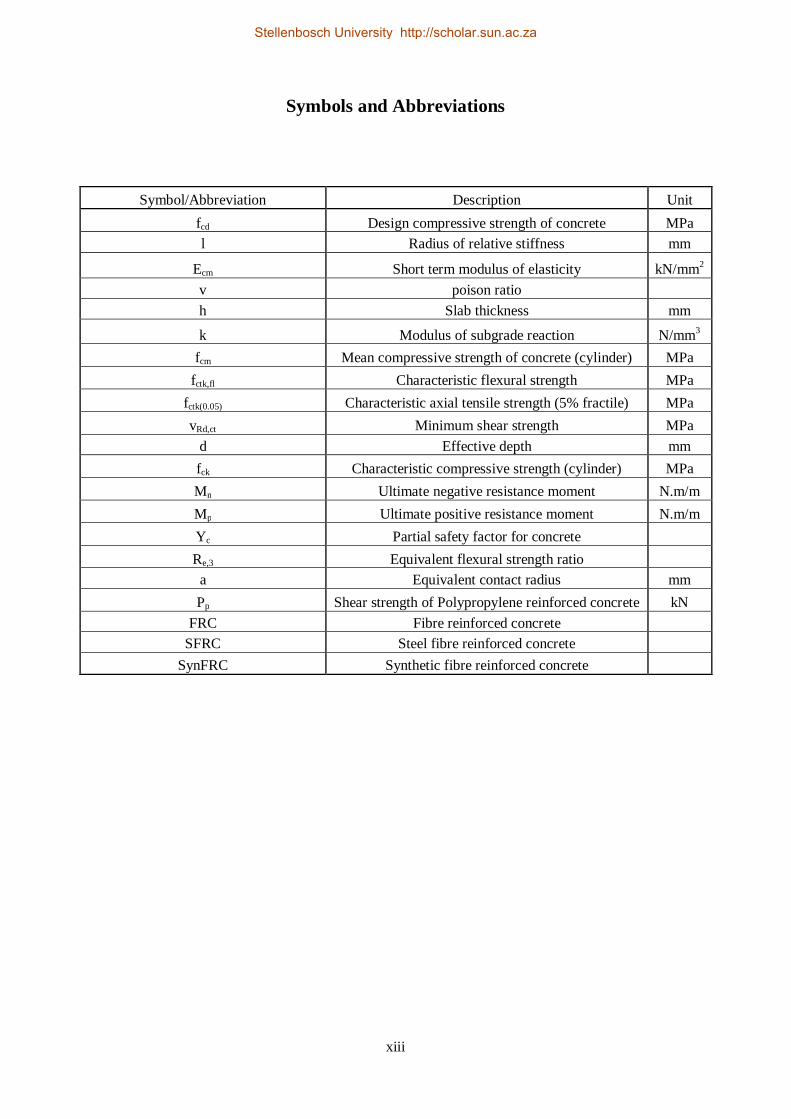
Symbols and Abbreviations
Symbol/Abbreviation Description Unit fcd Design compressive strength of concrete MPa l Radius of relative stiffness mm
Ecm Short term modulus of elasticity kN/mm2 v poison ratio
h Slab thickness mm
k Modulus of subgrade reaction N/mm3 fcm Mean compressive strength of concrete (cylinder) MPa
fctk,fl Characteristic flexural strength MPa fctk(0.05) Characteristic axial tensile strength (5% fractile) MPa vRd,ct Minimum shear strength MPa
d Effective depth mm fck Characteristic compressive strength (cylinder) MPa Mn Ultimate negative resistance moment N.m/m Mp Ultimate positive resistance moment N.m/m Yc Partial safety factor for concrete
Re,3 Equivalent flexural strength ratio
a Equivalent contact radius mm Pp Shear strength of Polypropylene reinforced concrete kN
FRC Fibre reinforced concrete
SFRC Steel fibre reinforced concrete
SynFRC Synthetic fibre reinforced concrete
Stellenbosch University http://scholar.sun.ac.za

1
Concrete is a well known and widely used construction material with particular characteristics which
influence the way in which it is used. Most of the modern day infrastructure is built from concrete.
This could be attributed to the relative ease of using concrete in construction since there are numerous
design codes and guidelines for its use. Concrete is known for its compressive resistance, but lacks
tensile strength. Plain unreinforced concrete also fails in a brittle manner once its compressive-,
tensile- or flexural resistance has been exceeded. Although much care can be given to the design and
construction of concrete structures, concrete remains a brittle material and as a consequence cracks
will occur at some stage. These cracks appear on the surface and throughout the depth of members
typically as a result of shrinkage, creep or overloading of a specific member.
Currently steel reinforcement is used as the conventional method in practice to enhance the
characteristics of concrete. Although it is both an effective and widely used method, the use of steel
reinforcement could be costly because of the price as well as time consuming from a construction
point of view (Manolis et al. 1997).
Alternatively fibres can be used to enhance the properties of concrete. Various different have been
used fibres and tested for its efficiency to improve the brittle nature of concrete (Banthia et al., 1995)
(Zollo, 1997).
The use of macro synthetic fibres to improve the structural behaviour of concrete is investigated in
this study. The main advantage of adding macro-synthetic fibres to concrete is the increase in post-
crack ductility. Many applications exist for the use of synthetic fibre reinforced concrete (SynFRC)
(Concrete Society UK TR 65, 2007). Typical applications include concrete for tunnel linings,
industrial- and domestic floors, swimming-pool construction and road pavements. The focus of this
investigation is on the use of SynFRC for industrial slabs on grade.
Large amounts of funds are allocated each year to the design and construction of concrete on grade
structures for example industrial floors, airport runways and roads. Typically designers use
empirically determined charts to derive a design thickness of such structures. This often leads to
overdesign which have negative consequences on the economical feasibility of such structures
Chapter 1. Introduction
Stellenbosch University http://scholar.sun.ac.za

2
(Baumann & Weisgerber, 1983) (Sorelli et al., 2006). Analytical design methods can also be used to
determine slab thicknesses.
The two methods currently used for the design of floors on grade are the Westegaard theory and the
Yield-Line theory (Barros & Figueiras, 2001) (Belletti et al., 2008). These methods are distinctly
different from a structural design point of view. The Westegaard theory was derived from elastic
theory while the Yield-Line theory includes the plastic behaviour of a concrete slab (Elsaigh et al.,
2005) (Soutsos & Lampropoulos, 2012). These two methods are discussed and used to determine the
effect of polypropylene fibres on the thickness design of slabs on grade.
The research methodology used included experimental and analytical investigations. The analytical
section uses both design theories for determining thicknesses of slabs on grade and comparisons are
drawn between the two theories. The experimental section consists of two parts. The first part
determines material properties of SynFRC by conducting tests on beam- and cube specimens. In the
second part large scale slab tests are performed to verify the accuracy of the design theories.
This study has two main objectives. The first is to investigate the mechanical properties of SynFRC
and its use in design theories for slabs on grade. The second objective is to compare the Westegaard
theory and the Yield-Line theory to each other in terms of design accuracy and efficiency for
determining slab thicknesses.
A possible outcome of this study would be to be able to advise industry on which materials to use in a
concrete mix design in combination with a specific design theory to obtain the most structurally sound
and economically feasible design thickness for a ground supported slab.
The report has the following layout: Chapter 2 gives the literature review conducted to gain
knowledge on the use of fibres in concrete. Chapter 3 shows a literature review of the two design
theories investigated in this report. In Chapter 4 a conceptual design is done by using both design
theories to obtain a thickness for a typical storage facility with a ground supported concrete slab. This
chapter includes the use of SynFRC in its design with the Yield-Line theory. Chapter 5 discusses the
tests performed to obtain values for design parameters of SynFRC. Chapter 6 explains the large scale
tests that were performed and shows the results from those tests. In Chapter 7 the results obtained
from the previous chapters are compared to the predicted values from the two design theories and the
accuracy of these methods are analysed. Chapter 8 concludes the findings of this research and gives
recommendations for future studies.
Stellenbosch University http://scholar.sun.ac.za
3
Fibre reinforced concrete (FRC) is not a new concept. Since biblical times fibres have been used in
cementing construction materials in the form of straw and horse hair (Brandt, 2008). In more recent
times the asbestos fibre was used extensively in structural components for example wall panels, roofs
and gates to name a view. In the early 1960’s the health risk of manufacturing and using asbestos
fibres became apparent and alternative fibres were introduced as a replacement (Labib & Eden, 2006).
After asbestos fibres, steel fibres was one of the first possible alternatives to steel bar reinforcing, with
the first patent being applied for in 1874. It was however only in the early 1970’s that the use of these
fibres on a large scale was noticed in the USA, Japan and in Europe. Characteristics that make FRC
more suitable than conventional reinforced concrete include post-crack ductility, time efficiency and
its ability to fill an irregular surface shape as found in tunnel construction (Tiberti et al., 2008)
(Bernard, 2000). Examples of existing structures build from steel and other fibre reinforced concretes
include ground supported slabs, suspended slabs, pile supported slabs, tunnel panel segments (The
Channel Tunnel Rail Link project) and various insitu concrete structures such as a 210m long, 6m
high is 310mm thick wall in Belgium (Concrete Society UK TR 63, 2007).
Synthetic fibres have been used successfully in railway- and road tunnels in Japan in sprayed concrete
linings. The 22km liyama Rail Tunnel was constructed with 52 000m3 of fibre reinforced concrete.
The Strood and Higham railways were relined with 900m3 of sprayed concrete. Typical fibre dosages
used was in the region of 9kg of synthetic fibres per cubic meter of concrete (Concrete Society UK
TR 65, 2007). Currently typical dosages of synthetic fibres for use in slabs on grade range from 2
to7kg/m3. Micro synthetic fibres are often used in combination with macro fibres to provide means for
reducing plastic shrinkage cracking (Aly et al., 2008) (Won et al., 2008).
2.1 Fibre Materials and Types
The desired result of adding fibres to any concrete mix is to enhance its mechanical and volumetric
stability. The improvements gained by using fibres depend on the properties of the fibre which
include the fibre material as well as fibre length and geometry.
Chapter 2. Fibre Reinforced Concrete
Stellenbosch University http://scholar.sun.ac.za

4
Various materials are used to produce fibres for use in concrete. Currently the main distinctly
different categories are steel fibres, synthetic fibres, glass fibres and organic- or natural fibres.
Table 2.1 shows some of the fibres from every category along with the basic material properties.
Manufacturers produce fibres in different geometrical forms to improve the bond characteristics
between fibre and the concrete matrix while trying to prevent fibre bundling from occurring during
the mixing process. Figure 2.1 shows some of the common fibre geometries for steel fibres.
Table 2.1: Properties of various fibre types (Zollo, 1995) (Shah, 1971).
Specific gravity Tensile strength (Mpa) Elastic Modulus (GPa)
Acrylic 1.16-1.18 296-1000 14-19 Aramid I 1.44 2930 62 Aramid II 1.44 2344 117 Carbon I 1.9 1724 380 Carbon II 1.9 2620 230
Nylon 1.14 965 5 Polyester 1.34-1.39 228-1103 17
Polyethylene 0.92-0.96 76-586 5- 117 Polypropylene 0.9-0.91 138-690 3.0-5.0 Alkali-resistant 2.7-2.74 2448-2482 79-80
Non Alkali-resistant 2.46-2.54 3103-3447 655-72 Coconut 1.12-1.15 120-200 19-26
Sisal - 276-568 13-26 Bagasse 1.2-1.3 184-290 15-19
Steel 7.8 1000-3000 200 Glass 2.6 2000-4000 80
All fibres are either categorised as macro- or micro fibres. The term structural fibres are often used for
macro fibres which have lengths between 19 and 60mm (Concrete Society UK TR 63, 2007). These
fibres are expected to bridge cracks and provide structural support to the hardened state of concrete
(Won et al., 2009). Micro fibres on the other hand are included in a mix to help improve the fresh and
early-age tensile- and flexural strength of concrete (Pelisser et al., 2010). These fibres provide the
necessary resistance to tensile forces developed by drying shrinkage as well as plastic shrinkage.
Micro fibres range between 2- and10mm in length and nominal diameters of between 0.1and1mm
(Concrete Society UK TR 63, 2007).
The shapes of synthetic fibres are similar to that of steel fibres with the straight and crimped forms
being the most common for macro fibres. Micro fibres for both steel and synthetic fibres are usually
only available in short straight forms. Figure 2.2 shows example of polypropylene fibres, with micro
Stellenbosch University http://scholar.sun.ac.za

5
fibres at the top and the packs in which macro fibres are produced at the bottom. In this project
polypropylene fibres are used. These fibres could be produced as monofilaments, collated fibrillated
filaments or continues films (Zheng & Feldman, 1995). Polypropylene is the most commonly used
synthetic fibre for concrete. This is due to their light weight and relative low cost (Manolis et al.,
1997).
Polypropylene (PP) is made under low-pressure by using Ziegler-Netta catalysts. PP bares
resemblance to polyethylene and is also a linear hydrocarbon. Polypropylene’s micro-structure is
arranged in such a way that it promotes the formation of crystals. This leads to a better balance of
chemical resistance and heat stability which is influenced by molecular weight and polydispersity as
with all thermoplastics. Fibres are produced by drawing the PP into thin film sheets and then slitting it
in longitude to produce tapes which is then further worked into fine fibres that can either be collated
or held together in their length. These tapes are twisted along its lengths to produce fibre bundles and
these have a lower aspect ratio (Zheng & Feldman, 1995).
Figure 2.1: Steel fibre geometries (Concrete Society UK TR 63, 2007).
The British Standards (BS EN 14889- “Fibres for Concrete, Part 2: Polymer fibres – Definition,
specifications and conformity.”) classifies fibres made from polymeric materials into two classes
(Concrete Society UK TR 65, 2007). The classes are:
Stellenbosch University http://scholar.sun.ac.za

6
- Class I: Micro fibres
Class Ia: Micro fibres < 0.3mm in diameter, monofilament.
Class Ib: Micro fibres < 0.3mm in diameter, fibrillated.
- Class II: Macro fibres > 0.3mm in diameter.
It is also stated that Class II fibres are typically used when an increase in post-crack flexural strength
is needed i.e. increase in ductility (Concrete Society UK TR 65, 2007).
Figure 2.2: Examples of polypropylene micro- and macro fibres.
2.2 Mechanical Behaviour of FRC
In literature structural performance of FRC is often compared to that of concrete reinforced with steel
bar or steel mesh as a means to quantify relative structural performance. This is because of the level
of confidence that designers and contractors use the conventional method to improve the concrete’s
tensile and flexural resistance. In literature there have been many experimental investigations into
Stellenbosch University http://scholar.sun.ac.za

7
finding an alternative to this type of reinforcement (Li, 2002) (Ding & Kurstele, 1999). In the
following paragraphs some of the most relevant findings from literature are documented to compare
the performance of various types of FRC for their structural use. Although different fibre types will be
discussed, steel- and polypropylene fibre reinforced concrete are the main focus of this research.
Fibres begin to function in a structural supportive manner when the concrete matrix starts to crack.
The fibres then provide ductility and support by bridging cracks and thus providing post-crack
strength to the concrete. When performing a load to deflection test of any kind, it can typically be
noticed that by adding fibres to a mix there exists a strain softening material behaviour. This is the
term used when some loads can be supported after the concrete first begins to crack (typically the case
of synthetic fibres). Strain hardening is encountered when a higher load is reached after the concrete
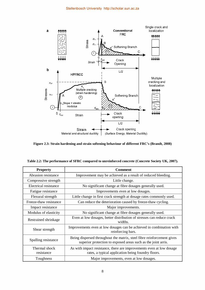
cracks for the first time, by the fibres bridging the cracks. Figure 2.3 demonstrates this strain softening
and hardening behaviour. Typically only high performance fibre reinforced concretes (HPFRCC)
show strain hardening (Brandt, 2008).
The toughness and thus the energy which could be absorbed by the addition of fibres could be
computed by determining the area under a stress-strain curve (obtained from flexural strength tests). It
is essential to understand that the first crack strength of a fibre reinforced specimen will not
necessarily give higher values than plain concrete. The effect of pull-out forces which is generated as
the fibres gradually slip out of the matrix causes the improved toughness. It is thus preferred that
pull-out of the fibres occur instead of the fibres breaking (fibre rupture). Fibre rupture is the result of
too large bond strength between fibres and the surrounding matrix. In order to achieve optimum
efficiency of the fibres, the bond strength between fibres and the matrix needs to be as close as
possible to the same value as the tensile strength of the fibres, but still less (Banthia, 1994).
Steel fibres are currently one of the most used fibres in concrete for the purpose of improving
structural performance. The Concrete Society of the United Kingdom documented guidelines for the
use of steel fibre reinforced concrete (SFRC) in their technical report No. 63 in 2007 (Concrete
Society UK TR 63, 2007). In this report they provide a framework for the design of structures like
slabs on various support structures, linings for tunnel construction and the design of insitu concrete
members. Table 2.2 shows the performance enhancing capabilities that steel fibres can provide
compared to unreinforced concrete according to the mentioned reference.
Stellenbosch University http://scholar.sun.ac.za
8
Figure 2.3: Strain hardening and strain softening behaviour of different FRC’s (Brandt, 2008)
Table 2.2: The performance of SFRC compared to unreinforced concrete (Concrete Society UK, 2007).
Property Comment Abrasion resistance Improvement may be achieved as a result of reduced bleeding.
Compressive strength Little change. Electrical resistance No significant change at fibre dosages generally used. Fatigue resistance Improvements even at low dosages. Flexural strength Little change in first crack strength at dosage rates commonly used.
Freeze-thaw resistance Can reduce the deterioration caused by freeze-thaw cycling. Impact resistance Major improvements.
Modulus of elasticity No significant change at fibre dosages generally used.
Restrained shrinkage Even at low dosages, better distribution of stresses can reduce crack widths.
Shear strength Improvements even at low dosages can be achieved in combination with reinforcing bars.
Spalling resistance Being dispersed throughout the matrix, steel fibre reinforcement gives superior protection to exposed areas such as the joint arris.
Thermal shock resistance
As with impact resistance, there are improvements even at low dosage rates, a typical application being foundry floors.
Toughness Major improvements, even at low dosages.
Stellenbosch University http://scholar.sun.ac.za

9
In the TR 65, Guidance on the use of Macro-synthetic-fibre-reinforced Concrete, Concrete Society
UK (2007) (hereafter referred to as TR 65), it is explained that even though synthetic fibres were
tested in concrete since the 1960’s, only recently fibres made from these materials began to show
desired structural support. This is due to new technologies in the production of synthetic fibres where
higher modulus fibres are being made (2-10GPa) with improved anchorage between the fibres and the
matrix. The problems encountered from lower modulus fibres (1-2GPa) were a result of poor bond
strength between the fibres and the concrete matrix which was further weakened by the high Poisson
ratio of the fibres. Typically synthetic fibres are used up to a maximum volume fraction of 1.35%
(12kg/m3) (TR 65, Concrete Society UK, 2007).
The specific mechanics involved with the flexural- and tensile behavior of fibre reinforced concrete is
more complex than that of conventional elastic beam theory and thus it cannot be used to determine
the structural response of FRC accurately after cracks forms. Even for plain concrete there exists a
difference in stress to strain behavior between bending tests and uni-axial tensile tests. In the case of
fibre reinforced concrete this difference is amplified due to the quasi-plastic tensile behavior of the
composite. When the fibres start to bridge a crack, they apply point loads across the surface of the
cracked face. Each of these point loads varies in magnitude and orientation and as a result it is a
complex task to model the effect of each fibre individually (TR 65, Concrete Society UK, 2007).
Typically equivalent stress block is used to represent the response from the flexural behavior of the
fibres (Concrete Society UK TR 65, 2007). Figure 2.4 shows the stress blocks from both elastic
response and a one proposed to model FRC. In these models the concrete’s compressive response is
modelled as linear elastic and the tensile stress block for FRC is rectangular with the neutral axis at a
quarter of the depth. The neutral axis moves toward the compression section as soon as micro cracks
forms and the fibres are activated. It is assumed that fibre pull-out is the mechanism controlling the
tensile response along with the assumption of constant loads across cracks of small widths (Concrete
Society UK TR 65, 2007).
Researchers found varying results surrounding the performance of various FRC’s and polypropylene
fibre reinforced concrete in particular (Alhozaimy et al., 1995). Typically the standard properties
tested are compressive strength, flexural strength and indirect tensile strength.
Stellenbosch University http://scholar.sun.ac.za

10
Figure 2.4: Elastic stress block (left) and a proposed stress block for FRC (Concrete Society UK TR 65, 2007).
2.2.1 Flexural and Shear Strength of FRC
A study by Ding & Kurstele (1999) found that the early age flexural- and shear strength of SFRC
greatly out-performs that of unreinforced concrete of the same age and that it can replace steel mesh
reinforcement for underground construction. Flexural panel tests were conducted in accordance to the
European standard for panel tests for sprayed concrete as shown in Figure 2.5 (EFNARC) (Ding &
Kurstele, 1999).
The tests were conducted from an age of 10h up to 48h and it was found that the optimal dosage of
fibres that improves the flexural and shear capacity is 40kg/m³. It was also found that from a dosage
of 20kg/m³ of fibres and higher, the failure mode for a panel test changed from a punching shear
failure as for steel mesh reinforcement (SRC) to a flexural failure.
Stellenbosch University http://scholar.sun.ac.za

11
10 cm
50 c
m
60 c
m70
cm
10 c
m
Figure 2.5: Test set setup for panel tests according to EFNARC (Ding & Kurnele, 1999).
The research concluded from test results that the influence of SFRC is more contributing in the early
ages, green state, than it is for hardened concrete. This was found by comparing the load to deflection
curves for 20-, 40- and 60kg/m³ of steel fibres in a mix to that of the minimum amount of steel
reinforcement advised in building codes. The testing ages were 10h, 18h, 30h and 48 hours. It was
found that the 20kg/m³ dosage outperformed SRC at the age of 10 hours for its energy absorption
capacity. But from an age of 18 hours the SRC exceed the capacity provided by the fibres (Ding &
Kurstele, 1999). Figure 2.6 shows the load to deflection curves obtained in this particular study for an
age of 48 hours of the concrete panels.
Figure 2.6: Comparison of SRC to SFRC for different fibre dosages at an age of 48h (Ding & Kurstele, 1999).
Stellenbosch University http://scholar.sun.ac.za

12
Cengiz and Turanli (2005) performed similar panel tests to compare the performance of steel mesh
reinforcement to that of steel fibre reinforcement, high performance polypropylene fibre
reinforcement and a hybrid mix of both steel- and polypropylene fibres. Their most important
conclusions obtained were that polypropylene fibres greatly enhanced the flexural ductility, toughness
and load carrying capacity of the concrete. They further found that a hybrid polypropylene- and steel
fibre mix can be used alternatively to steel mesh in shotcrete applications to gain improvements in
mechanical properties. Figure 2.7 shows the comparison of a hybrid fibre reinforced mix to that of
high performance polypropylene fibres (HPPFR) of different dosages for a panel load-deflection
shotcrete test. 30kg/m³ of steel fibres and 5kg/m³ of polypropylene fibres were used in the hybrid fibre
mix and 10 kg/m³ and 7 kg/m³ were used for the two polypropylene mixes respectively (Cengiz &
Turanli, 2005).
Figure 2.7: Comparison of hybrid fibre reinforcement to HPPFR (Cengiz & Turanli, 2005).
An increase in flexural toughness was witnessed by Alhozaimy et al. (1995) in their research by
performing flexural strength tests on concrete specimens reinforced with polypropylene fibres. They
found that for volume fractions of 0.1%, 0.2% and 0.3% of fibres the flexural toughness increased by
44%, 271% and 386% respectively over that of plain unreinforced concrete for the same mix
compositions.
2.2.2 Tensile Strength of FRC
The splitting tensile strength of concrete can be increased by adding fibres to a concrete mix. During
their research Choi and Yuan (2005) found that glass fibre reinforced concrete (GFRC) and
polypropylene fibre reinforced concrete (PFRC) have a splitting tensile strength of 20 to 50% more
Stellenbosch University http://scholar.sun.ac.za

13
than that of unreinforced concrete (Figure 2.8). They also concluded that the splitting tensile strength
of these composites ranged between 9 and 13% of their compressive strengths (Choi & Yuan, 2005).
Figure 2.8: Comparison between splitting tensile strength of GFRC and PFRC with unreinforced concrete after Choi and Yuan (2005).
2.2.3 Compressive Strength of FRC
Since the compressive strength of concrete is one of its main attributes and the reason for adding any
reinforcing material is in most cases to improve the tensile properties, little focus has been put on the
compressive strength of FRC. Because compressive strength tests typically measure the load until
failure (first cracks) and since fibres only contributes to the structural integrity of concrete by bridging
cracks after cracks begins to form, the effect of fibres on compression strength is not its main
attribute.
Different and often contradicting results on compression strength tests are found in literature.
Alhozaimy et al. (1995) found in their research that the addition of low volumes (0.1%) of
polypropylene fibres to a concrete mix has no significant effect on the compressive strength of
conventional concrete. Previous research suggests that the compressive strength of concrete
1
1.5
2
2.5
3
3.5
4
0 10 20 30 40 50 60 70 80 90 100
Split
ting
tens
ile s
tren
gth
(MPa
)
Age at testing (days)
GFRC 1% fibres GFRC 1.5% fibres PFRC 1% fibres PFRC 1.5% fibres PC
Stellenbosch University http://scholar.sun.ac.za

14
containing synthetic fibres (0-0.3%) is less than that of plain concrete (Zollo, 1984). Other studies
found that by using 0.5% fibres by volume, the compressive strength could be increased by as much
as 25% (Mindess & Vondran, 1988). The addition of supplementary materials such as silica fume or
slag in combination with the use of fibres could yield some improvement in compressive resistance of
the composite (Alhozaimy et al., 1995). Figure 2.9 shows compression strength of specimens of
conventional concrete and that of mixed binder type with and without 0.1% fibres by volume.
Figure 2.9: Compressive strength of different concrete mixes comprising of plain and fibre reinforced concrete (Alhozaimy et al., 1995)
2.2.4 Fire Resistance and Durability
By bridging cracks, fibres stops or limits the propagation of cracks and also limits crack widths. These
attributes not only contributes to structural integrity, but also improves the durability of structures
made from such materials. Polypropylene fibres perform well as a measure to improve the fire
resistance of concrete since it has a low melting point (107-141°C), which is a desirable attribute.
During fire exposure, high temperatures cause the trapped water particles, still present in the concrete,
to turn into vapour and this result to pressures developing within the concrete. When these pressures
exceed the resistance of the concrete brittle failure can occur. When polypropylene fibres are present,
they melt and provide channels through which the vapour could escape (Ali et al., 2004) (Kodur et al.,
2003). Synthetic fibres and more specifically polyolefins (polypropylene and polyethylene) have
35.233.1
43.4
32.4
36.5
32.4
44.8
34.5
0.0
5.0
10.0
15.0
20.0
25.0
30.0
35.0
40.0
45.0
50.0
Com
pres
sive
Str
engt
h (M
Pa)
Binder Type
Vf = 0 %
Vf = 0.1 %
Stellenbosch University http://scholar.sun.ac.za

15
shown to be durable when used as fibres in concrete, since it is less susceptible to the aggressive
agents that attack concrete (Concrete Society UK, TR 65, 2007).
2.2.5 Impact Resistance of FRC
Impact resistance refers to the strength provided by the concrete when exposed to a high strain rate.
Fibre reinforced concrete is known to have an increased resistance to impact loading over that of
unreinforced concrete. In literature there is no unique standard or specific test that can be performed
to determine impact resistance (Banthia et al., 1989). One method used for testing impact resistance is
to subject a concrete sample to a dynamic load from a drop weight system (Mindess & Vondran,
1988) (Wang et al., 1996). Other methods include the use of a pendulum to subject an impact load and
the use of high velocity projectiles (Zhang et al., 2007). The testing method that is chosen depends on
the conditions to which the concrete will be exposed to. For concrete structures like warehouse floors,
the drop weight system should be sufficiently accurate to simulate loading conditions. For more
extreme loadings, for example impacts from high velocity projectiles such as bullets or explosive
fragments, other methods should be used to simulate the actual conditions.
Mindess & Vondran (1988) found in their research that polypropylene fibres with a length of 19.1mm
which were added in volume fractions from 0.1% to 0.5% increased impact resistance and fracture
energy of the concrete. The experimental method used was a 345kg drop hammer released from 0.5m
above the concrete specimen. Beam specimens of 1200mm in length, 100mm wide and 125mm deep
were used. From the tests they found that an increase in fracture energy and impact resistance
occurred as the volume fraction of fibres in the mix increased. At a dosage of 0.5% fibres a maximum
bending load, as a measure of impact strength, was obtained which was 40% higher than that of plain
concrete. They also noticed that the fracture energy doubled at this volume of fibres. The primary
mode of failure was fibre rupture rather than fibre pull-out (Mindess & Vondran, 1988).
In another similar study the effect of adding polypropylene fibres as well as steel fibres were tested to
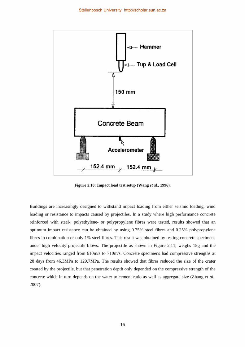
determine whether an increase in impact resistance can be achieved (Wang et al., 1996). For this
study beam specimens were tested under a dynamic load from a drop hammer (60.3kg). Figure 2.10
shows the schematic test setup. This study found that polypropylene fibres improved impact loading
resistance marginally (21% increase at 0.5% volume of fibres). When steel fibres were used at the
same volume fraction an increase of 41% in impact resistance was noticed. This study also concluded
that the mechanism of failure changed from fibre rupture to fibre pull-out as the volume fraction
approached the region of 0.5% to 0.75%. Below this region rupture of the fibres is the dominating
mode of failure and for greater volumes of fibres a pull-out mechanism occurs (Wang et al., 1996).
Stellenbosch University http://scholar.sun.ac.za
16
Figure 2.10: Impact load test setup (Wang et al., 1996).
Buildings are increasingly designed to withstand impact loading from either seismic loading, wind
loading or resistance to impacts caused by projectiles. In a study where high performance concrete
reinforced with steel-, polyethylene- or polypropylene fibres were tested, results showed that an
optimum impact resistance can be obtained by using 0.75% steel fibres and 0.25% polypropylene
fibres in combination or only 1% steel fibres. This result was obtained by testing concrete specimens
under high velocity projectile blows. The projectile as shown in Figure 2.11, weighs 15g and the
impact velocities ranged from 610m/s to 710m/s. Concrete specimens had compressive strengths at
28 days from 46.3MPa to 129.7MPa. The results showed that fibres reduced the size of the crater
created by the projectile, but that penetration depth only depended on the compressive strength of the
concrete which in turn depends on the water to cement ratio as well as aggregate size (Zhang et al.,
2007).
Stellenbosch University http://scholar.sun.ac.za

17
Figure 2.11: Projectile for impact testing (Zhang et al., 2007).
2.3 Concluding Summary
According to the information provided in the paragraphs above, it is clear that the addition of fibres to
concrete improves its mechanical behaviour. The way in which synthetic fibres can be used to
improve the mechanical behaviour of slabs on grade is further investigated in the following chapters.
Stellenbosch University http://scholar.sun.ac.za

18
Slabs on grade refer to concrete slabs supported by a substructure of soil and/or other natural
materials. The term ‘slab’ refers to one concrete section, typically seen as the sections created
by casting or saw-cutting. The term ‘floor’ refers to the entire space covered by the concrete
slabs. The main difference between most design methods for slabs on grade is the way in which the
soil support is incorporated. Two distinctly different models of soil support are found in literature.
These are the Winkler support system and the elastic-isotropic solid model (ACI Committee, 2006)
(Concrete Society UK, 2003). The term Winkler soil is used to describe a soil’s behaviour as
providing constant vertical support, deflecting only vertically and proportional to the load applied
(ACI Committee, 2006). This type of soil support can be viewed as linear springs providing
independent support to a structure in the vertical direction. An elastic support model on the other hand
assumes that an area of soil which undergoes deflection will affect the surrounding soil by displacing
it accordingly (Marais & Perrie, 1993).
The classical design theories used in practice can be categorised by being either elastic or elastic-
plastic. In the early 1920’s Westegaard developed an elastic theory for the thickness design of slabs
on grade and modelled the supporting soil by using the Winkler model. He viewed the concrete slab
as homogeneous, isotropic and elastic. Good correlations between experimental values and values
computed from Westegaard’s theory were found at Arlington, Virginia Experimental Farm and the
Iowa State Engineering Experiment Station (ACI Committee, 2006). In 1943 Burmister proposed a
theory based on an elastic-solid support structure. It was called a layered-solid theory for rigid
pavements. He proposed that a concrete slab should be treated as having infinite dimensions in the
horizontal plane, but a finite thickness. The theory considered limited deformation under loading
conditions. This theory was never developed further because of the lack of considering corner- and
edge loading conditions (ACI Committee, 2006).
The Yield-Line theory is based on plastic theory which considers the structural behaviour of a
concrete slab not only in the elastic region, but also includes resistance to moments and forces in the
plastic region. Losberg first proposed this theory in 1961 by considering displacements that are not
proportional to applied loads. This method consists of finding the critical formation of lines on a slab
where yielding is expected and then determining the support provided after cracks occurred. If fibres
Chapter 3. Design of Slabs on Grade
Stellenbosch University http://scholar.sun.ac.za

19
were included in a concrete mix, the post-crack ductility provided by it could be calculated by this
theory. In 1986 Rao and Singh used rigid plastic behaviour with square criteria of failure for concrete
to predict the collapse load. In 1962 Meyerhof used plastic theory to derive equations for ultimate
loads for the interior, edge and corner regions of slabs on grade. The Meyerhof and Rao & Singh
design principles are similar, with the exception that the Meyerhof equations do not account for shear
forces in the concrete (Concrete Society UK, 2003).
All the above mentioned theories can be classified according to the type of model on which they are
based to describe the behaviour of both the slab and the subgrade. These models are: elastic-isotropic
solids, thin elastic slabs and the thin elastic-plastic slab model (ACI Committee, 2006).
Numerical models are often used as an alternative to the above mentioned theories by performing a
finite element analysis on a concrete slab supported by an elastic foundation. Non-linear fracture
mechanics can also be used to model the concrete’s behaviour and resistance to moments and forces
as cracks forms and propagates.
In this project the Westegaard theory and the Yield-Line theory are investigated further as these
methods are most common in practice (Barros & Figueiras, 2001). More specifically, the two theories
will be investigated as they are documented in design guides namely Concrete Industrial Floors on
the Ground by Marais & Perrie (1993) and Concrete Industrial Ground Floors, Technical Report No.
34 by the Concrete Society UK (2003) respectively. It is necessary to understand the aspects
surrounding the construction of industrial floors by considering all the components of their design.
The first part of this chapter discusses these aspects while the second part deals with the design
theories.
3.1 Subgrades and Subbases
Both the Yield-Line theory and the theory of Westegaard use the Winkler soil model. The so-called k-
value is often used to represent the support provided by a Winkler soil and have units of pressure per
unit displacement (also called the modulus of subgrade reaction). Typical k-values for some of the
most common soils are listed in Table 3.1. The k-value of a soil can be determined on-site by
performing a simple test (with Eq. 3.1). Marais and Perrie (1993) states that the pressure (kPa) at
which a 760 mm diameter bearing plate deflects 1.27mm is divided by 1.27 to give the k-value
(kPa/mm or N/mm3) using the following:
Stellenbosch University http://scholar.sun.ac.za

20
푘 = ( ) ..
(3.1)
Table 3.1: Typical k – values for different soil types (Concrete Society, 2003).
Soil type k value (N/mm3)
Lower value
Upper value
Fine or slightly compacted sand 0.015 0.03
Well compacted sand 0.05 0.1 Very well compacted sand 0.1 0.15
Loam or clay (moist) 0.03 0.06 Loam or clay (dry) 0.08 0.1
Clay with sand 0.08 0.1 Crushed stone with sand 0.1 0.15
Coarse crushed stone 0.2 0.25 Well compacted crushed stone 0.2 0.3
In Concrete Industrial Ground Floors, Technical Report No. 34 by the Concrete Society UK (2003),
it is stated that an approximation of the k-value is sufficient for design purposes, since it has a minor
effect on the error occurring in thickness design. It is stated that up to an error of 50% in the k-value
determination, the error occurring in the thickness design is only 5%. The support provided by a
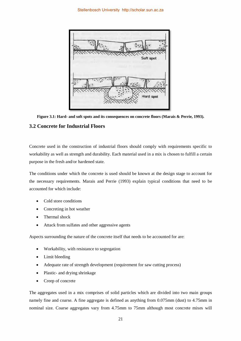
subgrade should however be of uniform nature, without hard and soft spots as shown in Figure 3.1.
The main purpose of a subbase is to provide uniform soil support for a slab when the subgrade has
some sort of irregularity. The two main types of subbases are those that are treated and those that are
not. A treated subbase means that cement was added to provide stability to the soil material. Thus is
the use of a subbase not always required since it is assumed to provide no extra support to the slab
(Marais & Perrie, 1993).
Stellenbosch University http://scholar.sun.ac.za
21
Figure 3.1: Hard- and soft spots and its consequences on concrete floors (Marais & Perrie, 1993).
3.2 Concrete for Industrial Floors
Concrete used in the construction of industrial floors should comply with requirements specific to
workability as well as strength and durability. Each material used in a mix is chosen to fulfill a certain
purpose in the fresh and/or hardened state.
The conditions under which the concrete is used should be known at the design stage to account for
the necessary requirements. Marais and Perrie (1993) explain typical conditions that need to be
accounted for which include:
Cold store conditions
Concreting in hot weather
Thermal shock
Attack from sulfates and other aggressive agents
Aspects surrounding the nature of the concrete itself that needs to be accounted for are:
Workability, with resistance to segregation
Limit bleeding
Adequate rate of strength development (requirement for saw cutting process)
Plastic- and drying shrinkage
Creep of concrete
The aggregates used in a mix comprises of solid particles which are divided into two main groups
namely fine and coarse. A fine aggregate is defined as anything from 0.075mm (dust) to 4.75mm in
nominal size. Coarse aggregates vary from 4.75mm to 75mm although most concrete mixes will
Stellenbosch University http://scholar.sun.ac.za

22
contain 19mm as largest nominal particle size (Owens, 2009). The characteristics of the aggregates
used in a concrete mix will determine the properties of the concrete in its fresh and hardened state. In
the fresh state, the grading along with the particle shapes and sizes will affect the workability of the
concrete. In the hardened state the strength and grading of the aggregates will contribute to the
strength and durability of the concrete. Deleterious substances found in some aggregates can cause
negative reactions within the concrete with consequences such as alkali-silica reaction and sulphate
attack. It is therefore important to use a trusted supplier of aggregates for use in concrete.
The binder type and composition is the main factor contributing to the development of strength in
concrete. Binder materials usually used in concrete is Original Portland cement as well as cement
replacing materials such as Fly Ash, Ground Granulated blast furnace and Silica Fume.
The cement particles, when hydrated by water, forms cementing compounds which acts as “glue”
between aggregates and cement paste. The reactions that take place during hydration are exothermic.
The main compound that provides strength to the hardened cement paste is calcium silicate hydrate
(C3S2H3), which is needle- and plate-like crystals. Cement replacing materials could be used to
partially replace ordinary Portland cement. These materials form cementing compounds by reacting
with calcium hydroxide (Ca(OH)2) and not by the process of hydration (Owens, 2009).
Ground granulated blast furnace slag (GGBS) also reacts with and in water to form cementing
compounds where the reaction is alkali activated. Pozzolanic materials used as cement extenders in
South Africa are mainly fly ash (FA) and condensed silica fume (CSF). These binder materials do not
react with water to form cementing compounds, but react with calcium hydroxide in water to produce
these compounds. For both pozzolanic materials and GGBS the principal compound providing
strength is calcium silicate hydrate (Owens, 2009).
Each of these cement replacing materials provide specific attributes for their use in concrete. The
most common advantages of using these materials are to lower the heat of hydration (except silica
fume) and to increase early age strength as well as long term strength. They also provide for better
durability against aggressive environments (attacks from various agents) and improve the properties
of fresh concrete. The type of binder material used in a mix, its fineness and the ratio to which it is
used compared to the water content will determine its effect on the strength of the concrete. As the
water to binder ratio decreases, the strength of the concrete increases (Owens, 2009).
Admixtures are used to improve properties like workability and strength development. Admixtures,
which alter the structure of the concrete, could also be used. Typical admixtures such as plasticisers,
super plasticisers (both for workability) and air entrainment admixtures are commonly used in the
flooring industry.
Stellenbosch University http://scholar.sun.ac.za

23
3.3 Joints in Floors
To minimise the possibility of cracks occurring on surfaces due to shrinkage and other induced forces,
joints are placed at specific intervals to divide a large area of concrete into smaller sections to control
the stresses on a smaller scale. Joints can be made by saw-cutting or by casting techniques. The first
type is referred to as sawn joints and the latter is called formed-joints. Each of these types of joints
can either be free-movement joints or restrained-movement joints. Other joints that are found in
practice are isolation detail and tied joints (Concrete Society UK, 2003).
The purpose of a free-movement joint is to provide load transfer between slabs without restraining the
slabs against horizontal movement from induced stresses. Typical mechanisms used for this type of
joints are round or square dowels with a sleeve attached to it to allow horizontal movement. Plates of
various sizes and shapes across joints are also used with success. Figure 3.2 shows these transfer
mechanisms, where the top two illustrations shows dowels and the bottom one shows the use of a
plate system. No reinforcement is provided across a free-movement joint (Concrete Society UK,
2003).
Restrained-movement joints allow a limited amount of movement across the joint. This type of joint is
characterized by reinforcement that is continuous across joints. Reinforcement is designed to allow
limited horizontal and lateral movement while providing load transfer for vertical forces. Typically
steel fabric and smooth or deformed bars are used to achieve this characteristics as shown in
Figure 3.3 and Figure 3.4.
Stellenbosch University http://scholar.sun.ac.za

24
Figure 3.2: Transfer mechanisms across formed free-movement joint (Concrete Society, UK, 2003).
Figure 3.3: Sawn restrained-movement joint with the use of steel fabric (Concrete Society UK, 2003).
Tied joints are also designed like restrained-movement joints with the exception of the allowance for
any kind of movement. These joints are often used as a construction method rather as a structurally
planned design (Concrete Society UK, 2003).
Stellenbosch University http://scholar.sun.ac.za

25
Figure 3.4: Tied or restrained-movement joint (Concrete Society UK, 2003).
“Isolation details” is the term used to describe the method used to isolate a floor area from any
elements which could provide a restraint and so causing stresses to occur when loads are applied to
the floor. These elements could be columns, bases for machinery, walls or any element which could
provide restraint. This type of joint usually includes the use of an elastic material to separate the floor
from a restraining member.
Aggregate interlock also provides load transfer between joints by the mechanism of friction. Typical
load transfer mechanisms as described in the paragraphs above provides for 25 to 50% of force that
can be transferred between adjoining slabs (Marais & Perrie, 1993) (Concrete Society, UK, 2003).
3.4 Typical Loads
Typical loads that are considered in the design process can be categorized as being either static or
dynamic of nature. The static loads that need to be accounted for is pallet racking loads (point loads),
line-loads from internal walls, and distributed loads commonly found in general storage spaces. The
loads that are often the detrimental factors surrounding the design thickness of a floor are the dynamic
loads. These are inflicted by material handling equipment normally found in industrial buildings. The
small wheels from forklift trucks often inflicts the most damage to a concrete floor since it carries
heavy loads and the small wheels does not distribute these loads in a sufficiently uniform manner,
especially at the edge and corner regions of a slab.
Stellenbosch University http://scholar.sun.ac.za

26
Typically the design layout of an industrial floor will attempt to minimize loads at corners and edges
of slabs to avoid stress concentrations from forming in those regions.
3.5 The Westegaard Theory
By using the theory of Westegaard, the assumption is made that the concrete will be subjected to
loading in the elastic region of material behavior only. Any crack that occurs is seen as failure of the
slab. The equations developed by Westegaard has been modified over the years and most design
guides only provide design charts derived from the original equations. The main source of literature
available and used in South Africa is Concrete Industrial Floors on the Ground by Marais and Perrie
(1993). In this document design charts are provided for the thickness design of slabs subjected to
point loads, dynamic loads and distributed loads.
The objectives of this design guide are to account for the following aspects:
Preventing excessive flexural stresses from occurring to avoid cracking
Preventing localizes failure such as punching shear from occurring due to concentrated loads
Minimize and prevent excessive deflections from subgrade settlement
Preventing failure due to overload by designing for sufficient bearing capacity (Marais &
Perrie, 1993)
Examples of the equations used to draw up the charts found in most design guides are given below.
They are known as modified Westegaard equations as well as elastic Westegaard and Timoshenko
equations. These equations can be used to determine the maximum stress occurring at a corner, edge
or internal region of a slab due to a patch load. A patch load is typically a circular area on the surface
of a slab subjected to a load from a vehicle’s wheel (Knapton, 2005).
For a load on an interior region:
휎 = 0.275(1− 휇)푃..
(3.2)
For a load on an edge region:
휎 = 0.529(1− 0.54휇)푃..
(3.3)
And for a load at a corner the maximum stress is given by:
Stellenbosch University http://scholar.sun.ac.za

27
휎 = ⎝
⎜⎜⎛
⎝
⎜⎛ .
.
⎠
⎟⎞
.
⎠
⎟⎟⎞
(3.4)
where
σ = Maximum flexural stress (MPa)
P = Point load (kN)
h = Slab thickness (mm)
E = Elastic modulus (MPa)
k = Modulus of subgrade reaction (N/mm3)
b = Radius of contact zone (mm)
μ = Poisson’s ratio
In Marais and Perrie’s (1993) design guide point loads, dynamic loads and distributed loads are dealt
with by designing for the most critical loading situation for each of these load types. For dynamic
loads, the load exerted by industrial trucks is seen as the most critical loading condition. Point loads
are dealt with by designing for the post loads from racks. Dynamic loads and point loads are generally
the determining factors in thickness design due to the relative small areas on which loads are applied.
Typically a designer checks the all ready determined thickness for its capacity to resist forces caused
by distributed loads. The spacing of aisles and their widths are a detrimental parameter contributing to
the distributed load capacity of a slab.
3.5.1 Point Loads
Loads from racks, which support great amounts of products and goods, can often cause failure of a
slab due to the concentration of the load on a small base-plate. This failure is often caused by
excessive bearing- or shear forces and not by flexural stresses. The three main aspects determining the
thickness of a slab for a given point load are: The magnitude of the load, the size of the area of
loading and spacing of the point loads. In Concrete Industrial Floors on the Ground by Marais and
Perrie (1993), design charts are given for three different values of modulus of subgrade reaction. Each
of the three charts uses both the longitudinal and lateral spacing of rack legs as design inputs. The
other parameters used in the charts are the maximum post load design for, the maximum flexural
strength of the concrete and the contact area of the post load. For the flexural strength parameter, a
Stellenbosch University http://scholar.sun.ac.za
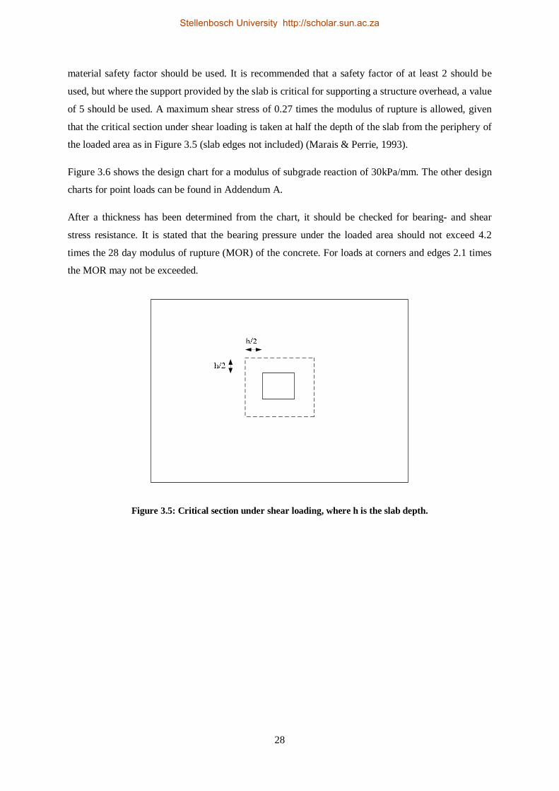
28
material safety factor should be used. It is recommended that a safety factor of at least 2 should be
used, but where the support provided by the slab is critical for supporting a structure overhead, a value
of 5 should be used. A maximum shear stress of 0.27 times the modulus of rupture is allowed, given
that the critical section under shear loading is taken at half the depth of the slab from the periphery of
the loaded area as in Figure 3.5 (slab edges not included) (Marais & Perrie, 1993).
Figure 3.6 shows the design chart for a modulus of subgrade reaction of 30kPa/mm. The other design
charts for point loads can be found in Addendum A.
After a thickness has been determined from the chart, it should be checked for bearing- and shear
stress resistance. It is stated that the bearing pressure under the loaded area should not exceed 4.2
times the 28 day modulus of rupture (MOR) of the concrete. For loads at corners and edges 2.1 times
the MOR may not be exceeded.
Figure 3.5: Critical section under shear loading, where h is the slab depth.
Stellenbosch University http://scholar.sun.ac.za

29
Figure 3.6: Design chart for post loads and a k-value of 30kPa/mm (Marais & Perrie, 1993).
Stellenbosch University http://scholar.sun.ac.za
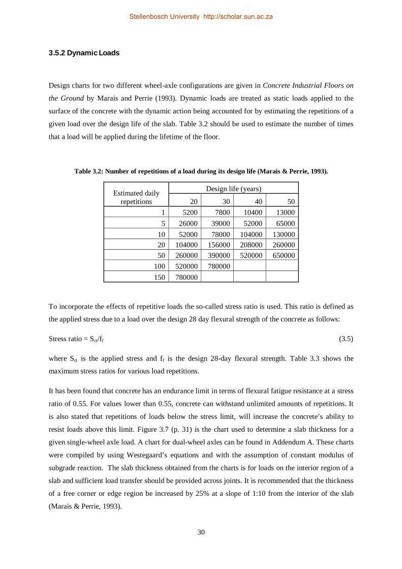
30
3.5.2 Dynamic Loads
Design charts for two different wheel-axle configurations are given in Concrete Industrial Floors on
the Ground by Marais and Perrie (1993). Dynamic loads are treated as static loads applied to the
surface of the concrete with the dynamic action being accounted for by estimating the repetitions of a
given load over the design life of the slab. Table 3.2 should be used to estimate the number of times
that a load will be applied during the lifetime of the floor.
Table 3.2: Number of repetitions of a load during its design life (Marais & Perrie, 1993).
Estimated daily repetitions
Design life (years)
20 30 40 50 1 5200 7800 10400 13000 5 26000 39000 52000 65000
10 52000 78000 104000 130000 20 104000 156000 208000 260000 50 260000 390000 520000 650000
100 520000 780000 150 780000
To incorporate the effects of repetitive loads the so-called stress ratio is used. This ratio is defined as
the applied stress due to a load over the design 28 day flexural strength of the concrete as follows:
Stress ratio = Sct/ff (3.5)
where Sct is the applied stress and ff is the design 28-day flexural strength. Table 3.3 shows the
maximum stress ratios for various load repetitions.
It has been found that concrete has an endurance limit in terms of flexural fatigue resistance at a stress
ratio of 0.55. For values lower than 0.55, concrete can withstand unlimited amounts of repetitions. It
is also stated that repetitions of loads below the stress limit, will increase the concrete’s ability to
resist loads above this limit. Figure 3.7 (p. 31) is the chart used to determine a slab thickness for a
given single-wheel axle load. A chart for dual-wheel axles can be found in Addendum A. These charts
were compiled by using Westegaard’s equations and with the assumption of constant modulus of
subgrade reaction. The slab thickness obtained from the charts is for loads on the interior region of a
slab and sufficient load transfer should be provided across joints. It is recommended that the thickness
of a free corner or edge region be increased by 25% at a slope of 1:10 from the interior of the slab
(Marais & Perrie, 1993).
Stellenbosch University http://scholar.sun.ac.za

31
Table 3.3: Maximum stress ratios for various load repetitions (Marais & Perrie, 1993).
Total load repetitions Stress ratio
unlimited 0.5
400 000 0.51
300 000 0.52 200 000 0.54 100 000 0.56 50 000 0.59 30 000 0.6 10 000 0.64 2 000 0.7 1 000 0.73
3.5.3 Distributed Loads
In Concrete Industrial Floors on the Ground by Marais and Perrie (1993), it is stated that the two
aspects that need to be checked when designing for a distributed load is cracking in unloaded areas
due to negative bending moments and excessive settlement of the subgrade (Marais & Perrie, 1993).
Tables, which gives maximum allowable loads for a given floor thickness and subgrade k-value, can
be found in this reference. The so-called Hetenyi equations were used to compile the design tables.
These tables (Addendum A) deal with two design conditions, namely a situation where the loading
conditions and layout is known and one where it is not.
The tables can be used to check a certain design thickness for its distributed load capacity rather than
to arrive at a design thickness for a load. For a variable layout configuration, the following equation is
given to determine the distributed load capacity of an industrial floor slab:
푊 = 0.33푆 √ℎ푘 (3.6)
where
W = Load capacity (kPa)
Sct = Maximum flexural stress of the concrete (MPa)
h = Thickness of the slab (mm)
and k is the modulus of subgrade reaction (kPa/mm) (Marais & Perrie, 1993)
Stellenbosch University http://scholar.sun.ac.za
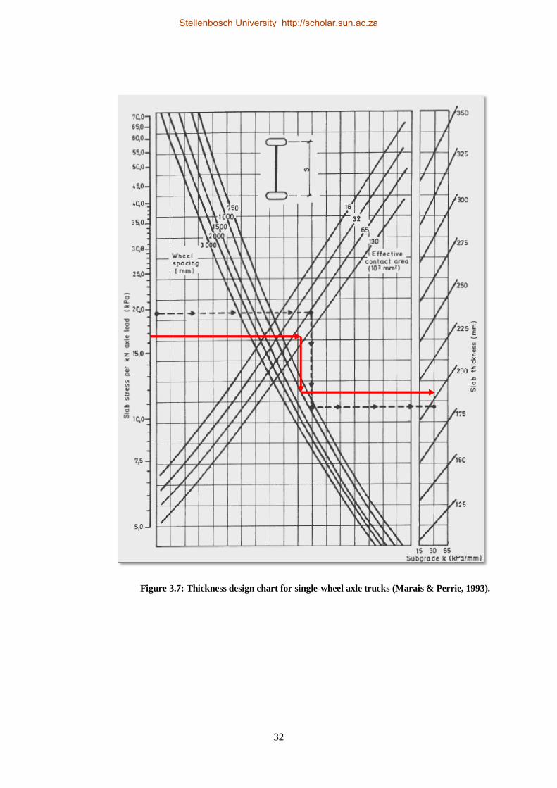
32
Figure 3.7: Thickness design chart for single-wheel axle trucks (Marais & Perrie, 1993).
Stellenbosch University http://scholar.sun.ac.za

33
3.6 The Yield-Line Theory
The Yield-Line theory assumes that cracking does occur and provides means for determining
moments caused by loading by assessing the patterns of the yield-lines. These moments are then used
in calculations to compute the design thickness of a floor. The choice of yield-line patterns affects the
efficiency of this method and it depends on the user to determine the most critical pattern. The most
common use of this method is for suspended floors. Figure 3.8 demonstrates some typical yield-line
patterns for the given point loads. Concrete Industrial Ground Floors, Technical Report No. 34 by the
Concrete Society UK (2003) (hereafter referred to as TR 34), is used as basis for the demonstration of
the Yield-Line theory in this report. All equations and design aspects discussed below are from this
reference. The structural advantages of using fibres are captured in this method where the equivalent
flexural strength ratio is used to incorporate the ductility provided by them.
Figure 3.8: Examples of yield-line patterns for point loads on a concrete floor (Concrete Society, 2003).
The Yield-Line theory is a plastic theory as previously mentioned. This implies that the post-crack
strength of the concrete is taken into consideration in determining the thickness of a slab. This is done
by incorporating the ductility provided by fibres or other types of reinforcement. When a load is
applied to a concrete floor, positive- and negative bending moments develop. The positive bending
moments causes sagging yield-lines on the bottom surface of a slab and the ductility of the
reinforcement provides additional strength to the concrete. For fibre reinforced concrete, when these
sagging moments cause cracks on the bottom of a slab, the fibres bridge these cracks and provides
ductility to the slab. This is the ductility which is incorporated in the design equations. Negative
moments (hogging moments) cause stresses to develop on the upper surface of the concrete and if
these stresses exceed the resisting capacity of the concrete, cracks will form. The occurrence of cracks
on the top surface is seen as failure of the slab, and for determining the hogging resistance of a slab
(a) Dual point loads (b) Quadruple point loads
Stellenbosch University http://scholar.sun.ac.za
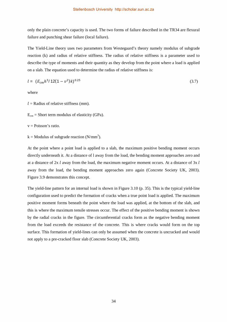
34
only the plain concrete’s capacity is used. The two forms of failure described in the TR34 are flexural
failure and punching shear failure (local failure).
The Yield-Line theory uses two parameters from Westegaard’s theory namely modulus of subgrade
reaction (k) and radius of relative stiffness. The radius of relative stiffness is a parameter used to
describe the type of moments and their quantity as they develop from the point where a load is applied
on a slab. The equation used to determine the radius of relative stiffness is:
푙 = (퐸 ℎ /12(1 − 푣 )푘) . (3.7)
where
푙 = Radius of relative stiffness (mm).
Ecm = Short term modulus of elasticity (GPa).
v = Poisson’s ratio.
k = Modulus of subgrade reaction (N/mm3).
At the point where a point load is applied to a slab, the maximum positive bending moment occurs
directly underneath it. At a distance of l away from the load, the bending moment approaches zero and
at a distance of 2x 푙 away from the load, the maximum negative moment occurs. At a distance of 3x 푙
away from the load, the bending moment approaches zero again (Concrete Society UK, 2003).
Figure 3.9 demonstrates this concept.
The yield-line pattern for an internal load is shown in Figure 3.10 (p. 35). This is the typical yield-line
configuration used to predict the formation of cracks when a true point load is applied. The maximum
positive moment forms beneath the point where the load was applied, at the bottom of the slab, and
this is where the maximum tensile stresses occur. The effect of the positive bending moment is shown
by the radial cracks in the figure. The circumferential cracks form as the negative bending moment
from the load exceeds the resistance of the concrete. This is where cracks would form on the top
surface. This formation of yield-lines can only be assumed when the concrete is uncracked and would
not apply to a pre-cracked floor slab (Concrete Society UK, 2003).
Stellenbosch University http://scholar.sun.ac.za

35
Figure 3.9: The significance of the radius of relative stiffness, 푙 (Concrete Society UK, 2003).
The following equation gives the capacity of moment resistance of a concrete slab to withstand tensile
flexural forces:
푀 = 푓 , (ℎ /6) (3.8)
where M is the moment per unit length (kNm/m), 푓 , is the characteristic flexural strength of plain
concrete (N/mm2) and h is the thickness of the slab (mm).
The Yield-Line theory incorporates the ductility provided by fibres or other types of reinforcement by
using the effective flexural strength ratio, Re,3. The TR 34 uses the Japanese Standard to determine the
amount of energy or equivalent post first-crack strength that is achieved by a beam specimen
(Concrete Society UK, 2003). Figure 3.11 shows a typical result from a flexural test. The equivalent
flexural strength (fe,3) of the concrete, according to the Japanese Standard, is determined by
performing a four-point bending test and using the average value of load applied to deflect a beam
3mm over a span of 450mm.
Stellenbosch University http://scholar.sun.ac.za

36
Negative
Positive
Positive moment producing first bottom crack at the limit of the elastic rangeElastic
Plastic
Circumferential cracks produced by negative
moments Mn Radial cracks produced by
positive moments Mp
P
P
Figure 3.10: Yield lines from a true point load (Concrete Society UK, 2003).
Figure 3.11: Determining equivalent flexural strength from a load-deflection curve (Concrete Society UK, 2003).
Stellenbosch University http://scholar.sun.ac.za

37
The ratio between the equivalent flexural strength and the first-crack strength is called the equivalent
flexural strength ratio, Re,3:
(3.9)
where, Re,3 is the equivalent flexural strength ratio
fe,3 = Equivalent flexural strength, MPa
ffc = Stress at first crack, MPa
By using fibres, additional moment capacity is gained from the fibres and this is incorporated in the
design by calculating the residual positive bending moment Mp. The Re,3 value needs to be at least 0.3
in order to be used in the equation below, otherwise the equivalent flexural strength provided is not
sufficient (Concrete Society UK, 2003).
(3.10)
The ultimate negative bending moment in the concrete is given by Mn:
(3.11)
For loads at the interior, edge or corners of a slab, different equations are used to determine the load
capacity. The different zones i.e. interior, edge and corners are defined in Figure 3.12.
Figure 3.12: Definition of the location of different load regions (Concrete society UK, 2003).
Stellenbosch University http://scholar.sun.ac.za

38
In Figure 3.12, a = equivalent contact radius (mm) and 푙 = radius of relative stiffness.
It has been stated in the TR 34 that when sufficient transfer of forces is provided between slabs the
corner loading should be treated as an edge loading (Concrete Society UK, 2003). The advantage of
increased ductility from fibres is obtained in the calculations of load capacity in the interior and the
edges of slabs when the values of Eq. 3.10 and 3.11 are added together:
푃 = 2휋(푀 + 푀 ) (3.12)
where Pu is the ultimate true point load (a = 0) capacity (kN).
The load capacities obtained from the TR 34’s Yield-Line equations are based on the assumption that
the ductility provided is sufficient so that shear failure does not occur first.
The way in which the Yield-Line theory’s equations are applied to a design problem is discussed in
Chapter 4 where a conceptual design is discussed. Unlike the Westegaard’s design charts, the Yield-
Line theory does not give a value for the thickness required for a given load directly. The process of
obtaining the correct value is done by trial and error, where the thickness of a slab is assumed at the
beginning of the process.
3.7 Concluding Summary
The Westegaard theory uses elastic theory while the Yield-Line theory uses plastic theory to derive
design thicknesses of floors on grade. The two theories are investigated further in the following
chapters to determine their design accuracy for the use of synthetic fibre reinforced concrete floors on
grade.
Stellenbosch University http://scholar.sun.ac.za

39
The design steps taken for both the Westegaard theory and the Yield-Line theory are explained in this
chapter by using a fictional design problem. The specific design parameters and requirements are
different for the two theories and since the design guidelines of these two methods largely rely upon
empirical data, a practical demonstration will best illustrate the use of them. This study is performed
to compare the thickness designs from the two theories to each other and for this reason only the
thicknesses are designed and no additional details such as transfer-joints. The structure under
consideration is shown in the Figure 4.1. This could be seen as a typical storage facility where various
loading conditions are applied.
Figure 4.1: Typical industrial storage facility layout.
This facility will be housing general goods in racks and maize in the distributed loading area shown in
plan. There are two entrances through which motorized vehicles could enter the building, one on the
east side and one on the south side. There are also two doors through which the building could be
entered with one on the south- and one on the west side.
Chapter 4. Conceptual Slab Design
Distributed Load
R
a
c
k
i
n
g
Racking
2.5m post
spacing
1.5m post spacing 40m
120m
Stellenbosch University http://scholar.sun.ac.za

40
The 40x120m floor will be constructed using three 40x40m pours. This floor is jointless as drying
shrinkage is not considered as it would not influence the design thickness. The footings of the racks
are 224x224mm base plates and are spaced at 1.5m and 2.5m in the lateral and longitudinal directions
respectively. Table 4.1 shows the properties of the soil- and concrete that are used in the floor design.
Table 4.1: General soil and concrete parameters.
Description Symbol Value Unit
Soil Modulus of subgrade reaction k 30 kPa/mm
California Bearing Ratio CBR 4 %
Concrete Design compressive strength of concrete fcd 30 MPa
Poison’s ratio v 0.2
Loads that are considered for this design is a 30kN/m2 distributed load, rack loads for the storage of
pallets (60kN/footing) and wheel loads from material handling equipment such as delivery trucks
(118kN/axle).
Polypropylene fibres will be added to the concrete mix when the Yield-Line theory is used as design
method. This fictional design is done to determine the effect of the addition of these fibres for various
values of the equivalent flexural strength ratio (Re,3). Note that fibres will have no effect on the design
using Westegaard’s theory as this method assumes no cracking and fibres only have an influence after
the concrete has cracked.
The design process for each method is explained at the hand of one worked example for each applied
load condition.
4.1 Thickness Design with Westegaard’s theory.
The load conditions that need to be designed for are point loads, dynamic loads and distributed loads.
The literature used to represent the Westegaard theory is Concrete Industrial Floors on the Ground
by Marais and Perrie (1993). All the equations used in this chapter are from this source.
Stellenbosch University http://scholar.sun.ac.za

41
4.1.1 Design for Post Loads
Table 4.2 gives the information required in the design for a post load of 60kN.
Table 4.2: Input data for 60kN post load.
Post load input longitudinal "Y" spacing 2500 mm transverse "X" spacing 1500 mm
Post load 60 kN Plate width 224 mm Plate length 224 mm
Load contact area 50 x103mm2 Load periphery 896 mm
The flexural strength of the concrete can be determined by using the following equation. Marais and
Perrie (1993) recommend that this equation be used to determine the flexural strength when the
flexural strength of the concrete is not tested under laboratory conditions.
ff = 0.62 x √fc (4.1)
with,
ff - Average flexural strength (MPa)
fc - 28 day average compressive strength (MPa)
The flexural strength for concrete used in this design was determined from Eq. 4.1 as 3.8MPa by
using an average strength of 38MPa (fc) for the 30MPa (design strength) concrete mix (Marais &
Perrie, 1993). The concrete stress is determined by using a safety factor of 2 when including the
flexural strength in the design charts such as Figure 3.6 this becomes:
Concrete stress = 3.8/2 = 1.9MPa
Figure 3.6 shows the design chart used to determine the slab thickness for a soil with a modulus of
subgrade reaction of 30kPa/mm. Similar figures can be found in Concrete Industrial Floors on the
Ground for k-values of 15kPa/mm and 55kPa/mm and are shown in Addendum A.
Figure 3.6 is entered with the post load of 60kN. At the intersection with the load contact area of
50x103mm2 move left right to concrete stress of 1.9MPa. From this point move upwards to the
intersection with the “Y”-spacing of 2500mm and then left to the intersection with the “X”-spacing of
Stellenbosch University http://scholar.sun.ac.za

42
1500mm. From this point move upward to a slab thickness of approximately 195mm. These steps are
shown in Figure 3.6 (red lines).
To check whether the load contact area was large enough, Figure 4.2 is used to determine the effective
contact area. It was found that the area is large enough. If this was not the case, the effective area from
Figure 4.2 would be used in Figure 3.6 to arrive at better estimation of slab thickness.
Figure 4.2: Effective contact areas for small loading areas (Marais & Perrie, 1993).
Now that a thickness is known it is necessary to perform a structural check on the design thickness of
the floor by computing the bearing capacity and shear stresses expected in the slab.
Stellenbosch University http://scholar.sun.ac.za
43
Bearing capacity
Allowable stress:
The allowable bearing stress for an interior-load is 4.2 times the concrete’s flexural strength and half
of it for an edge loading. This is:
Interior: 4.2 x ff = 4.2 x 4 = 16.8MPa (4.2)
Edge or corner = 2.1 x ff = 2.1 x 4 = 8.4MPa (4.3)
Computed stress:
Post load/contact area = 60 x103/50x10-3 = 1.20MPa (4.4)
This means that the bearing resistance of the slab is sufficient since 1.20MPa is smaller than 8.4MPa
and 16.8MPa.
Shear stresses
Allowable shear stress:
Marais & Perrie (1993) recommends that a shear capacity of 0.27 times the flexural strength at
28 days should be used. This becomes:
0.27 x ff = 0.27 x 4 = 1.08MPa (4.5)
This maximum stress should now be checked for interior-, edge- and corner loading conditions.
Interior:
= [( ) ( )] (4.6)
=∗( ∗ )
= 0.184 푀푃푎
Edge:
= [ . ∗( ) ∗( )] (4.7)
=∗( . ∗( ) ∗ )
= 0.29 푀푃푎
Stellenbosch University http://scholar.sun.ac.za

44
Corner:
= ∗[ . ∗( ) ( )] (4.8)
=∗( . ∗ )
= 0.48 푀푃푎
Since all the computed shear stresses are less than the allowable stress of 1.08MPa, the slab thickness
is sufficient to resist shear forces.
Thus a thickness of 195mm can be used.
4.1.2 Design for Wheel Loads (Single-wheel axle load)
Table 4.3 gives information needed to use the tables and figures provided in Concrete Industrial
Floors on the Ground by Marais and Perrie (1993) for thickness design of dynamic loads.
Table 4.3: Input data of design parameters dynamic loads (118kN axle load).
Dynamic loads (i.e. forklift trucks and other machinery) Axle load 118 kN
Wheel spacing (between two inner wheels) 1000 mm Nr. of wheel on axle 2
Tyre inflation pressure 700 kPa Nr. of daily repetitions 100
Design life 30 years
The general principle is to obtain a design thickness for a specific load by estimating the amount of
times which this load will be applied to the floor over its design life. Table 3.2 should be used to
estimate the number of repetitions of a load during the lifetime of the floor.
To incorporate the effects of repetitive loads the so-called stress ratio is used. This ratio is defined as
the applied stress due to a load over the design 28 day flexural strength of the concrete.
Stress ratio = Sct/ff (4.9)
Stellenbosch University http://scholar.sun.ac.za

45
where
Sct = Applied stress (MPa)
ff = Design 28-day flexural strength (MPa)
Table 3.3 gives the maximum stress ratios for various load repetitions.
From Table 3.2 the number of load repetitions can be determined as 780 000. This is used in Table 3.3
to obtain a stress ratio of 0.5.
The maximum flexural stress is thus 0.5x4 = 2MPa.
The contact area of a tyre is determined by dividing the load on a wheel by the tyre inflation pressure.
This is:
Contact area= ((118)(1000)(1000))/(2(700)) (4.10)
= 84.28571 x103mm2
The slab stress is determined by dividing the maximum stress allowed in the slab by the load of the
axle and its units is in kPa/(kN axle load) (Marais & Perrie, 1993). This is:
Slab stress = (2/118)*1000 = 16.9kPa/(kN axle load) (4.11)
Figure 3.7 shows the design chart for determining the thickness of a floor for single-wheel axle loads.
A similar chart that can be used to design for double-wheel axle loads can be found in Addendum A.
The chart is entered with the value of the slab stress. Move right to the effective contact area and then
down to the spacing of the wheels as given in Table 4.3.
From this chart the value of 210mm is read of as design thickness. Figure 3.7 shows graphically how
this chart was used by the indicated red lines.
The effective contact area of the tyre load needs to be checked by using Figure 4.2. By inspection it is
clear that the contact area is large enough and does not need to be adjusted.
The design thickness for the specified load is thus 210mm.
Stellenbosch University http://scholar.sun.ac.za

46
4.1.3 Distributed Loads
In Concrete Industrial Floors on the Ground by Marais and Perrie (1993) it is stated that the two
aspects that need to be checked when designing for a distributed load is cracking in unloaded areas
due to negative bending moments and excessive settlement of the subgrade.
Tables, which gives maximum allowable loads for a given floor thickness and subgrade k-value, can
be found in this reference. These tables deal with two design conditions, namely a situation where the
loading conditions and layout is known and one where it is not. It can thus be used to check a certain
design thickness for its distributed load capacity rather than to arrive at a design thickness for a load.
Since the governing factor from the calculations of the previous section is that of the wheel load, the
thickness of 210mm should be checked for its distributed load capacity.
From Tables A2 and A3 in Addendum A and by interpolating between the values from the two tables,
the maximum distributed load can be determined.
From Table A2 (k =20kPa/mm):
For a 200mm thick slab, the critical aisle width is 2.19m and the working load is 42.5kPa. For a
220mm thick slab, the critical aisle width is 2.36m and the working load is 44.5kpa. The critical aisle
width is 2.26m and the working load is 43.5kPa by interpolation for a 210mm thick slab.
From Table A3 (k = 40kPa/mm):
For a 200mm thick slab, the critical aisle width is 1.84m and the working load is 60kPa. For a 220mm
thick slab, the critical aisle width is 1.98m and the working load is 63kpa. The critical aisle width is
1.91m and the working load is 61.5kPa by interpolation for a 210mm thick slab.
For k = 30kPa/mm and h = 210mm the distributed load capacity is 52.5kPa by interpolation which is
more that the required 30kPa. The critical aisle width is 2.09m.
Final design thickness by using Westegaard’s theory
By using the principles and design equations of Westegaard, the design thickness for the given design
problem is 210mm.
Stellenbosch University http://scholar.sun.ac.za
47
4.2 Design with the Yield–Line Theory.
As for the design method of the Westegaard theory, the modulus of subgrade reaction is a governing
factor in the design equations for the Yield-Line theory method. All equations are from Concrete
Industrial Ground Floors, Technical Report No. 34 by the Concrete Society UK (2003) hereafter
TR 34.
As previously mentioned, synthetic fibres are used in the concrete for the design with the Yield-Line
theory. In order to include the ductility provided by the fibres, the equivalent flexural strength ratio
(Re,3) needs to be known and greater or equal to 0.3. This value is obtained by performing a four-point
bending test on the material. The equivalent flexural strength (fe,3) of a fibre reinforced mix is a
measure to quantify the post crack ductility provided by the fibres.
The Re,3 value chosen in this design was 0.33. This method starts by using an initial thickness as a first
attempt and then checking whether it is sufficient to carry the loads applied to the floor. If it is not
sufficient, a thicker value is tested until the slab thickness is sufficient to carry the applied loads. The
initial thickness used in this design is 145mm. The effect of transfer mechanisms between slabs is not
included in this design since its effect will be the same for both design theories.
The method starts by determining the parameters specific to the design approach. The first parameter
is the short term modulus of elasticity:
Ecm = 22 x (fcm/10)0.3 (4.12)
where
Ecm = Short term modulus of elasticity (GPa).
fcm = Mean compressive strength (cylinder) (MPa).
The mean compressive strength of a cylinder is given as 33MPa for a concrete grading of 30MPa by
the TR 34, therefore the short term modulus of elasticity is 31.475GPa. The radius of relative stiffness
is determined next with Eq. 3.7 and is 725.9mm. The characteristic flexural strength is determined
with:
fctk,fl = [1+(200/h)0.5]fctk(0.05) ≤ 2fctk(0.05) (4.13)
where
fctk,fl = Characteristic flexural strength (MPa).
fctk(0.05) = Characteristic axial tensile strength (5% fractile).
Stellenbosch University http://scholar.sun.ac.za

48
The TR 34 gives a value of 1.8MPa for fctk(0.05) when a concrete grade of 30MPa is used. The
characteristic flexural strength becomes:
fctk,fl = [1 + (200/145)0.5] x 1.8 ≤ 2 x 1.8
= 3.91 ≤ 3.6
= 3.6MPa
The most used and important parameter in the calculations of limit state design for various forms of
loads is the moment per unit length at which flexural tensile strength is reached. This moment is given
by Eq. 3.8. Partial safety factors should be used for the materials and for concrete (λc) a value of 1.5
was used for the ultimate limit state design, as recommended by the TR 34. The moment capacity of
the 145mm concrete slab is then:
M = (3.6/1.5) (1452/6) = 8410Nm/m or 8.41kNm/m
As stated earlier, by using fibres, additional moment capacity is gained from the fibres and this is
incorporated in the design by calculating the additional positive bending moment Mp by using
Eq. 3.10. This value is normally added to the negative moment capacity to achieve this purpose.
Mp = (3.6/1.5)(0.33)(1452/6)
= 2775.6Nm/m
The ultimate negative bending moment in the concrete is given by Eq. 3.11:
Mn = (3.6/1.5)(1452/6)
= 8410Nm/m
4.2.1 Point Loads
For a true point load the capacity is given by Pu (Eq. 3.12). For loads at the interior, edge or corners of
a slab, different load capacities exist. The different zones i.e. interior, edge and corners are defined in
Figure 3.12. The value for the ratio a/푙 is 0.174 with “a” the effective load contact radius (126.15mm)
and the radius of relative stiffness, 푙, is 725.9mm. The design capacities can now be calculated as
follow:
Stellenbosch University http://scholar.sun.ac.za

49
For interior loads:
When a/l = 0
Pu = 2π(Mp + Mn) (4.14)
= 2π(2.7756 + 8.410) = 70.28kN
When a/l > 0.2
Pu = 4π(Mp + Mn)/[1-a/3l] (4.15)
= 4π(2.7756 + 8.41)/[1-126.15/3(725.9)]
= 149.2kN
Interpolate for a/l = 0.174;
Pu = 138.86kN
For an free-edge load:
When a/l = 0
Pu = [π(Mp + Mn)/2] + 2Mn (4.16)
= [π(2.7756 + 8.41)/2] + 2(8.41)
= 34.39kN
When a/l > 0.2
Pu = [π(Mp + Mn) + 4Mn]/[1 – 2a/3l] (4.17)
= [π(2.7756 + 8.41) + 4(8.41)]/[1 – 2(126.15)/3(725.9)]
= 77.79kN
Interpolate for a/l = 0.174;
Pu = 72.1kN
For free corner loads:
When a/l = 0
Pu = 2Mn (4.18)
Stellenbosch University http://scholar.sun.ac.za

50
= 2(8.41)
= 16.82kN
When a/l > 0.2
Pu = 4Mn/[1-a/l] (4.19)
= 4(8.41)/[1-(126.15/725.9)]
= 40.716kN
Interpolate for a/l = 0.174;
Pu = 37.61kN
It is stated in the TR 34, that when sufficient transfer of forces is provided between slabs the corner
loading should be treated as an edge loading (Concrete Society UK, 2003). This means that the corner
load obtained is not the governing load case, but rather the edge load of 72.1kN
The concrete was reinforced with polypropylene fibres which provided an equivalent flexural strength
ratio of 0.33. The various loading conditions needed to satisfy a capacity of 72kN which is the rack
load (60kN) adjusted by a partial safety factor of 1.2 as is recommended by the TR 34. For a point
load of 60kN (rack load) a design thickness of 145mm is sufficient since all load capacities
determined exceed 72kN.
Figure 3.8 shows the yield-lines for a multiple point load configuration where “x” and “y” is the
spacing between loads. Equations 4.20 to 4.23 give the design load capacities for dual point loads and
quadruple point loads. If the centres of two point loads are less than a distance of twice the depth of
the slab away from each other, they can be seen as acting together. The magnitude of the load then
becomes the sum of the individual loads. The effective contact area becomes the sum of the two
contact areas expressed as circles plus the area between them (Concrete Society UK, 2003).
Figure 4.3 illustrates this effective load area.
Stellenbosch University http://scholar.sun.ac.za

51
Figure 4.3: Effective load contact area of two closely spaced loads (Concrete Society UK, 2003).
For dual-point loads:
When a/l = 0
Pu = [2π+ 1.8x/l][ Mp + Mn] (4.20)
When a/l > 0.2
Pu = [4π/(1-(a/3l))+ 1.8x/(l-(a/2))][ Mp + Mn] (4.21)
For quadruple-point loads:
When a/l = 0
Pu = [2π+ 1.8(x+y)/l][ Mp + Mn] (4.22)
When a/l > 0.2
Pu = [4π/(1-(a/3l))+ 1.8(x+y)/(l-(a/2))][ Mp + Mn] (4.23)
The lesser of the sum of the individual point loads, the sum of two dual-point loads or the value from
Equations 4.22 and 4.23 should be used as the ultimate load for quadruple-point loads.
Equations 4.20 to 4.23 estimates values for loads at the interior of a slab and to obtain the value for a
load at an edge, these values must be multiplied by 0.5. When the distance between the centres of
loads is greater than radius of relative stiffness, it can be assumed that they have little effect on the
load capacity at each other’s positions. For that reason multiple point loads were not used in this
design (Concrete Society UK, 2003).
Stellenbosch University http://scholar.sun.ac.za

52
Shear resistance
After it is confirmed that the edge and interior conditions has been satisfied, punching shear strength
needs to be checked. For synthetic fibre reinforced concrete the shear strength of the concrete is given
by the following equation and is the same as for plain concrete:
Pp = (0.035k13/2fck
1/2)u1d (4.24)
where
fck = Characteristic concrete compressive strength for a cylinder (25MPa for 30MPa concrete cube
strength (Concrete Society UK, 2003)).
d = Effective depth
k1 = 1 + (200/d)0.5 ≤ 2
u1 = Critical perimeter at distance twice the effective depth away from the loaded area.
Since the edge loading condition is critical the following parameters will be used:
uo = 3 x base plate dimension (length = width)
= 3 x 224 = 672mm
d = 0.75 x 145 = 108.75mm
fck = 25MPa
u1 = uo + π(2d)
=672 + π(2 x 108.75)
= 1355.3mm
k1 = 1+(200/108.75)0.5 ≤ 2
= 2.36 > 2
= 2
Pp = (0.035 x 23/2 x 251/2)1355.3 x 108.75
= 72.95kN
This concludes that the concrete has adequate shear resistance to resist the applied 60kN load.
Stellenbosch University http://scholar.sun.ac.za

53
4.2.2 Wheel Loads
Wheel loads are approached in the same way as point loads. The same equations will be used as for
point loads with the exception of the design for shear strength. For determining shear strength a
conservative assumption that half the contact area carries the full load at the edge of the slab is used.
This means that the load contact perimeter will effectively be a half circle, uo = π x a, where ‘a’ is the
equivalent contact radius.
The point load designed for is determined by factorising the wheel-axle load as follow:
P = 1.2 x 118/2 = 70.8kN
Table 4.4 (next page) shows the parameters used and Tables 4.5 and 4.6 gives the design ultimate
loads for a wheel load with a single-wheel axle load of 118kN. The determined thickness by trial and
error was found as 155mm. This thickness provides sufficient resistance to flexural and shear forces
applied anywhere on the slab to resist a force of 70.8kN. The critical factor was the shear strength
governing the design thickness for the wheel load.
4.2.3 Distributed Loads
In the TR 34 elastic theory is used to calculate the maximum allowed distributed load (kN/m2) and the
critical aisle width. The critical aisle width is the term used for that value of aisle width where the
maximum negative bending moments occur in the unloaded areas (Concrete Society UK, 2003).
The parameter λ is used to determine the critical aisle width and maximum allowed load. The inverse
of this parameter is known as the characteristic length of the system.
휆 =.
(4.25)
The critical aisle width is defined as π/2휆 and is found between two zones of distributed loads with a
width of π/휆 each.
The maximum allowable distributed load is determined by the following equation:
푤 = .
휆 푀푛 (4.26)
Subsequently the calculations for determining the capacity of the floor for a thickness of 155 mm are
shown in Table 4.7. It should be noted that the TR 34 recommends a reduction of 1.5N/mm2 in the
Stellenbosch University http://scholar.sun.ac.za

54
flexural strength used to determine the maximum load. This is done to account for forces experienced
from shrinkage and temperature fluctuations. Table 4.7 indicates that the slab should be sufficiently
thick to resist the applied 30kN/m2 load. The critical aisle width is 1.68m and thus aisles should be
either wider or narrower than this value to reduce bending moments in the unloaded areas.
Table 4.4: Calculation sheet of design thickness for a 118-kN axle wheel load.
Description Symbol and equation Value Unit Design compressive strength of
concrete fcd 16.67 MPa
Radius of relative stiffness l = (Ecm h3/12(1-v2 )k)0.25 763.13 mm
Short term modulus of elasticity Ecm = 22*(fcm/10)0.3 31.48 kN/mm2
poison ratio v 0.20
Slab thickness h 155.00 mm
Modulus of subgrade reaction k 0.03 N/mm3 Mean compressive strength of
concrete( cylinder) fcm (from TR 34 for 30MPa fcd) 33.00 MPa
Characteristic flexural strength fctk,fl =(1+(200/h)0.5)*fctk(0.05) ≤ 2*fctk(0.05) 3.60 MPa Characteristic axial tensile
strength (5% fractile) fctk(0.05) (from TR 34 for 30MPa fcd) 1.80 MPa
Minimum shear strength vRd,ct =0.035*k13/2fck1/2 0.49 MPa
k1 1+(200/d)0.5 ≤ 2 2.00 Effective depth d = 0.75*h 116.25 mm
Characteristic compressive strength (cylinder) fck (from TR 34 for 30MPa fcd) 25.00 MPa
Ultimate colapse load Pu 70.80 kN Ultimate negative resistance
moment Mn = (fctk,fl/ λc )(h2/6) 9610.00 Nm
Ultimate positive resistance moment Mp = (fctk,fl/ λc )(Re,3)(h2/6) 3171.30 Nm
Partial safety factor for concrete Yc 1.50
Equivalent flexural strength ratio Re,3 0.33
Equivalent contact radius a 163.80 mm a/l = 0.21
Table 4.5: Load capacities at the interior-, edge- and corner regions of the slab interpolated for a/l = 0.21.
a/l a/l a/l 0 >0.2 0.21 0 >0.2 0.21 0 >0.2 0.21
Internal Load (kN) Edge Load (kN) Corner Load (kN) 80.3 160.6 166.5 39.3 78.6 81.5 19.2 38.4 39.8
Stellenbosch University http://scholar.sun.ac.za
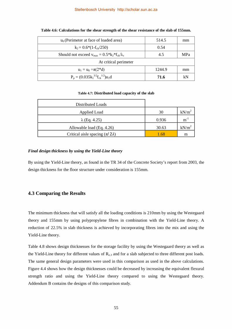
55
Table 4.6: Calculations for the shear strength of the shear resistance of the slab of 155mm.
u0 (Perimeter at face of loaded area) 514.5 mm
k2 = 0.6*(1-fck/250) 0.54
Should not exceed vmax = 0.5*k2*fck/λc 4.5 MPa
At critical perimeter
u1 = u0 +π(2*d) 1244.9 mm
Pp = (0.035k13/2fck
1/2)u1d 71.6 kN
Table 4.7: Distributed load capacity of the slab
Distributed Loads Applied Load 30 kN/m2
λ (Eq. 4.25) 0.936 m-1
Allowable load (Eq. 4.26) 30.63 kN/m2 Critical aisle spacing (π/2휆) 1.68 m
Final design thickness by using the Yield-Line theory
By using the Yield-Line theory, as found in the TR 34 of the Concrete Society’s report from 2003, the
design thickness for the floor structure under consideration is 155mm.
4.3 Comparing the Results
The minimum thickness that will satisfy all the loading conditions is 210mm by using the Westegaard
theory and 155mm by using polypropylene fibres in combination with the Yield-Line theory. A
reduction of 22.5% in slab thickness is achieved by incorporating fibres into the mix and using the
Yield-Line theory.
Table 4.8 shows design thicknesses for the storage facility by using the Westegaard theory as well as
the Yield-Line theory for different values of Re,3 and for a slab subjected to three different post loads.
The same general design parameters were used in this comparison as used in the above calculations.
Figure 4.4 shows how the design thicknesses could be decreased by increasing the equivalent flexural
strength ratio and using the Yield-Line theory compared to using the Westegaard theory.
Addendum B contains the designs of this comparison study.
Stellenbosch University http://scholar.sun.ac.za

56
Table 4.8: Westegaard- and Yield-Line theory’s estimation of slab thicknesses for three different point loads.
Thickness (mm)
Post Load (kN) Re,3 0 0.2 0.33 0.45
40 Westegaard theory 175 175 175 175 Yield-Line theory 125 120 115 110
50 Westegaard theory 185 185 185 185 Yield-Line theory 145 135 130 130
60 Westegaard theory 195 195 195 195 Yield-Line theory 160 150 145 145
Figure 4.4: The reduction in slab thickness with the increase in Re,3 values for three post loads.
In all cases, even without the incorporation of fibres, the Yield–Line theory predicts thinner slabs than
the Westegaard theory. When the Yield-Line theory is used the determining factor becomes the shear
resistance of the concrete even though the bending strength increases as the Re,3 values increases. This
is due to the fact that the Yield-Line theory does not incorporate the effect of synthetic fibres in the
calculations for shear resistance.
50
70
90
110
130
150
170
190
210
30 40 50 60 70
Slab
thic
knes
s (m
m)
Post Load (kN)
Yield-Line theory with Re,3 = 0Yield-Line theory with Re,3 = 0.2Yield-Line theory with Re,3 = 0.33Yield-Line theory with Re,3 = 0.45Westegaard theory for Re,3 = 0; 0.2; 0.33; 0.45
Stellenbosch University http://scholar.sun.ac.za
57
4.4 Concluding Summary
The effect of adding synthetic fibres to concrete is effectively incorporated in the thickness
determination of slabs on grade by using the Yield-Line theory. This theory predicts thinner slabs by
incorporating the ductility provided by fibres compared to the Westegaard theory which does not
incorporate any post-crack ductility. The ductility from the fibres is incorporated by using a flexural
strength ratio in the design with the Yield-Line theory. The question becomes then: what flexural
strength ratios can be achieved by synthetic fibre reinforced concrete and how accurate are the two
design theories? The following chapters deal with this by performing experimental- and analytical
investigations.
Stellenbosch University http://scholar.sun.ac.za

58
The experimental section of the project is divided into two parts. In the first section material
parameters were established by performing bending- and compressive strength tests on beam- and
cube specimens. The purpose of these tests is to determine the volume of polypropylene fibres that
needs to be added to the mix in order to achieve suitable Re,3 values. Four-point bending tests were
performed as stipulated in the Japanese Standard JSFC-SF4 (Concrete Society UK, 2003). The second
part of the experimental section (Chapter 6) discusses tests that were performed on slabs to determine
flexural bending strength.
5.1 Mix Design
Three different dosages of fibres were tested to determine an appropriate dosage which can be used in
slabs for industrial floors. Requirements such as workability, resistance to segregation, compressive
strength and tensile bending strength were taken into consideration. The three different dosages were
5kg/m3, 5.5kg/m3 and 6kg/m3 of macro polypropylene fibres. These fibre dosages correspond to
0.55%, 0.6% and 0.66% fibres per volume respectively. Table 5.1 shows the properties of the fibres
that were used in this project.
The mix was designed for a 28-day strength of 30MPa and a workability of more than 75mm was
desired. Table 5.2 shows the constituents of the three mixes. The superplasticiser dosage was adjusted
to satisfy the workability requirement. The water to cement ratio was 0.65. A plain concrete mix was
not designed or used in the tests of this chapter. The objective is not to compare the performance of
synthetic fibre reinforced concrete (SynFRC) to that of plain concrete in this chapter, but rather to
compare the performance of different dosages of fibres to each other.
Chapter 5. Experimental Tests on Material Parameters
Stellenbosch University http://scholar.sun.ac.za
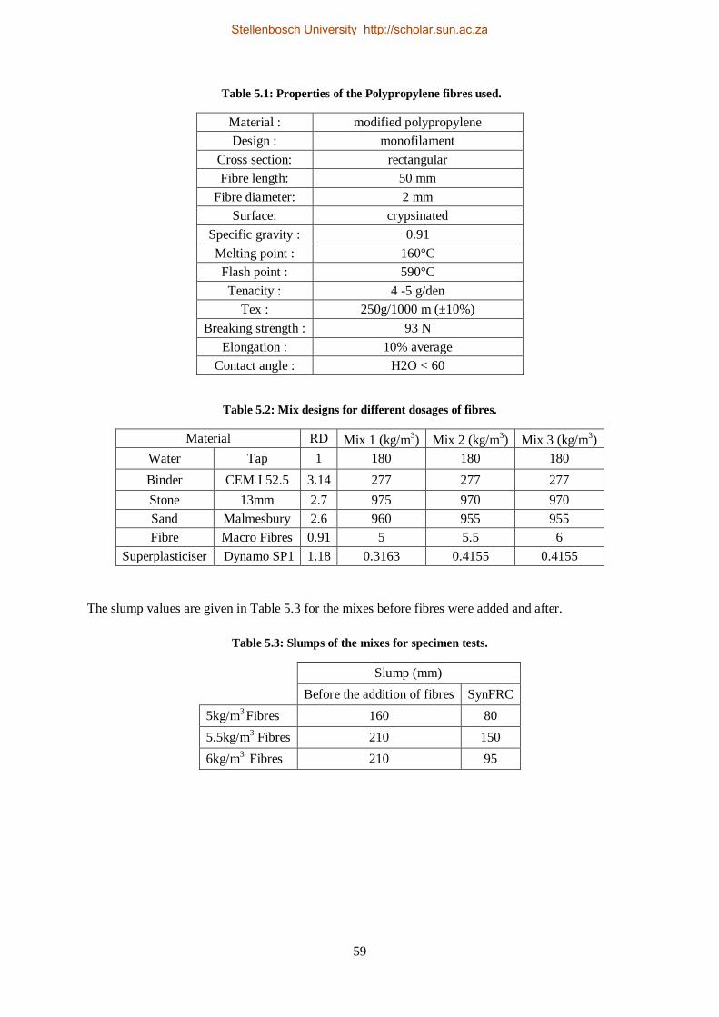
59
Table 5.1: Properties of the Polypropylene fibres used.
Material : modified polypropylene Design : monofilament
Cross section: rectangular Fibre length: 50 mm
Fibre diameter: 2 mm Surface: crypsinated
Specific gravity : 0.91 Melting point : 160°C
Flash point : 590°C Tenacity : 4 -5 g/den
Tex : 250g/1000 m (±10%) Breaking strength : 93 N
Elongation : 10% average Contact angle : H2O < 60
Table 5.2: Mix designs for different dosages of fibres.
Material RD Mix 1 (kg/m3) Mix 2 (kg/m3) Mix 3 (kg/m3) Water Tap 1 180 180 180 Binder CEM I 52.5 3.14 277 277 277 Stone 13mm 2.7 975 970 970 Sand Malmesbury 2.6 960 955 955 Fibre Macro Fibres 0.91 5 5.5 6
Superplasticiser Dynamo SP1 1.18 0.3163 0.4155 0.4155
The slump values are given in Table 5.3 for the mixes before fibres were added and after.
Table 5.3: Slumps of the mixes for specimen tests.
Slump (mm)
Before the addition of fibres SynFRC 5kg/m3 Fibres 160 80 5.5kg/m3 Fibres 210 150 6kg/m3 Fibres 210 95
Stellenbosch University http://scholar.sun.ac.za

60
5.2 Test Setup
The compressive strength was tested by testing four 100x100x100mm cubes according to SANS
5863:2006. Four-point bending tests, also known as loading at third points, were conducted on nine
beam specimens with three specimens per mix. The specimens measured 500x150x150mm. The four-
point bending test setup is shown schematically in Figure 5.1 and a photo is shown in Figure 5.2.
Figure 5.1: Schematical setup for four-point bending test.
The beam specimens were notched 25mm deep and 3mm wide at mid-span and were tested on a span
of 450mm as stated in the JSCE-SF4 (Concrete Society UK, 2003). Figure 5.2 shows the positioning
of an LVDT (linear variable displacement transducer) in a frame that was used to determine the
vertical deflection of the beams at mid-span. Two LVDT’s were used on each specimen, with one on
each side of the beam. The averages of the readings from the two LVDT’s were used as the
displacements at mid-span.
Stellenbosch University http://scholar.sun.ac.za

61
Figure 5.2: Four-point bending test setup with LVDTs as measuring devices.
5.3 Results
5.3.1 Compressive Strength
Table 5.4 shows the results from the cube tests.
Table 5.4: Compressive strength test results
Fibre dosages: 5 kg/m3 5.5 kg/m3 6 kg/m3 14 day Strength (MPa) 26.5 23.7 23.9 Coefficient of variance 0.027 0.05 0.039
5.3.2 Flexural Strength
Figure 5.3 to Figure 5.5 show the plots of flexural strength over deflection for the three mixes. The
flexural strength is calculated using:
σ = PL/bd2 (5.1)
With P the applied force, L the span, b the width and d, the notched depth, of the beam at mid-span.
Stellenbosch University http://scholar.sun.ac.za

62
Table 5.5 gives the average Re,3 values of the three mixes. The Re,3 values were taken from the graphs
of Figures 5.3 to 5.5 as shown in Figure 3.11. The average of all the flexural strength values up and
till a vertical displacement of 3mm at mid-span is determined. This value is then divided by the
modulus of rupture, i.e. the maximum flexural strength on the bending graphs, to obtain a Re,3 value.
Figure 5.3: Flexural strength results for beam specimens for 5kg/m3 fibre content
Figure 5.4: Flexural strength results for beam specimens for 5.5kg/m3 fibre content.
0.00
0.50
1.00
1.50
2.00
2.50
3.00
0 0.5 1 1.5 2 2.5 3
Flex
ural
str
engt
h(M
Pa)
Vertical deflection (mm)
0
0.5
1
1.5
2
2.5
3
3.5
0 0.5 1 1.5 2 2.5 3 3.5
Flex
ural
stre
ngth
(MPa
)
Vertical deflection (mm)
Stellenbosch University http://scholar.sun.ac.za
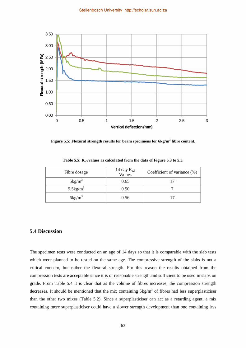
63
Figure 5.5: Flexural strength results for beam specimens for 6kg/m3 fibre content.
Table 5.5: Re,3 values as calculated from the data of Figure 5.3 to 5.5.
Fibre dosage 14 day Re,3 Values Coefficient of variance (%)
5kg/m3 0.65 17
5.5kg/m3 0.50 7
6kg/m3 0.56 17
5.4 Discussion
The specimen tests were conducted on an age of 14 days so that it is comparable with the slab tests
which were planned to be tested on the same age. The compressive strength of the slabs is not a
critical concern, but rather the flexural strength. For this reason the results obtained from the
compression tests are acceptable since it is of reasonable strength and sufficient to be used in slabs on
grade. From Table 5.4 it is clear that as the volume of fibres increases, the compression strength
decreases. It should be mentioned that the mix containing 5kg/m3 of fibres had less superplasticiser
than the other two mixes (Table 5.2). Since a superplasticiser can act as a retarding agent, a mix
containing more superplasticiser could have a slower strength development than one containing less
0.00
0.50
1.00
1.50
2.00
2.50
3.00
3.50
0 0.5 1 1.5 2 2.5 3
Flex
ural
str
engt
h (M
Pa)
Vertical deflection (mm)
Stellenbosch University http://scholar.sun.ac.za

64
(Owens, 2009). Another explanation could be that the fibres reduced the effective compaction thus
resulting in a lower strength.
The results from the bending tests show typical behavior of synthetic fibre reinforced concrete, as
explained in the TR 65, where the load-deflection curves show a strain softening behavior. The peak
load is reached as the modulus of rupture is reached (load at first crack). After this point the drop in
load capacity occurs over a longer deflection interval than for concrete containing the stiffer steel
fibres. As the fibres begin to bridge the cracks, an increase in load capacity occurs. It is typically the
case for macro-synthetic fibres to have a slow local increase in load capacity (after first-crack) as the
deflection increases up to the maximum post-peak strength (Concrete Society UK, TR 65, 2007).
Some irregularities that can be seen in some of the specimen tests can be due to a single fibre or fibre-
bundle rupturing. The Re,3 values from Table 5.5 suggests that the mix containing 5kg/m3 fibres
performed better in terms of post-crack ductility than the mixes containing higher volumes of fibres.
As mentioned, the lower superplasticiser content of this mix may have had an influence on it
developing strength more rapidly than the other two mixes, especially at such a relatively early age of
testing. It is also possible that the 5kg/m3 volume leads to better distribution of fibres, with minimal or
no fibre bundling although no bundling was observed for any of the mixes. One of the specimens
containing 5.5kg/m3 of fibres is suspected to have been cracked prior to testing (green line on
Figure 5.4). For this reason was that specific result ignored for further analysis. The coefficients of
variance of the different fibre dosages are sufficient to suggest that the results can be repeated with
relative confidence.
5.5 Concluding Summary
All the mixes yielded sufficient Re,3 values (>0.3) which can be used in the Yield-Line theory to
incorporate post-crack flexural strength in the design of concrete floors on grade. The mix containing
6kg/m3 of fibres was chosen to be used as the mix for the large scale tests. This decision was based on
the better workability of that mix, its high Re,3 value and also to test a higher volume fraction of fibres
to determine its practicality.
Stellenbosch University http://scholar.sun.ac.za

65
This section of the experimental program was undertaken to verify the design accuracy of the two
methods investigated in this project. The information from the previous chapters was used to
determine the thicknesses of the slabs, as well as the mix design that was used. The slabs had
dimensions of 2x2x0.12m. A thickness of 120mm was used since this is the lowest value that can be
found in the design charts of the literature used to represent the Westegaard theory. Two of the slabs
contained fibres and two were casted using plain concrete. The tests can be seen as having a dual
purpose, not only are two design theories tested for their accuracy, but also the effect that fibres have
on the flexural ductility of the concrete was determined.
6.1 Mix Design and Shuttering
The mix design was chosen based on the results of Chapter 5. As stated in the previous chapter, the
mix containing 6kg/m3 of fibres was chosen. A 120 liter pan mixer was used to mix five batches (100
liter each) of concrete to cast one slab. The available Malmesbury sand had a different grading as the
one used in the previous chapter. More superplasticiser was added to the mixes containing fibres due
to the change in the grading of the sand. Table 6.1 shows the mix design used for the slabs. The water
to cement ratio is 0.65.
The shuttering for the slabs was built from 21mm thick Pine plywood. The sides of the moulds were
reinforced with ribs to prevent the shuttering from deforming during the process of casting and to
support the weight of the concrete. One of the moulds is shown in Figure 6.1
Chapter 6. Large Scale Slab Tests
Stellenbosch University http://scholar.sun.ac.za

66
Table 6.1: Mix designs used in slab tests.
Material RD Plain concrete (kg/m3) Fibre reinforced concrete (kg/m3) Water Tap 1 180 180 Binder CEM I 52.5 3.14 277 277 Stone 13mm 2.7 970 970 Sand Malmesbury 2.6 955 955 Fibre Macro Fibres 0.91 0 6
superplasticiser Dynamo SP1 1.18 0.4155 1.247
6.2 Mixing- and Pouring Processes
The process of casting the slabs were done over four days, with one slab being cast per day. A poker-
vibrator was used to compact the concrete. After the mould was filled, the surface of the concrete was
floated to obtain a level surface finish. Four hooks, bended 12mm diameter reinforcing bars, were
placed in a slab, one close to each corner, to be able to lift the slabs into the testing position with a
crane. The slabs were cured for 14 days by using wet blankets to cover them. The blankets were kept
wet by saturating them with water each day.
Table 6.2 shows the average slumps of the concrete batches from the four slabs. Figure 6.1 shows one
of the synthetic fibre reinforced concrete (SynFRC) slabs on the day of casting and Figure 6.2 shows
the four slabs after they were cured for 14 days.
Table 6.2: Average measured slumps of the concrete used in slabs.
Slump (mm) Slab 1 (plain concrete) 170
Slab 2 (SynFRC) 140 Slab 3 (SynFRC) 155
Slab 4 (plain concrete) 190
During the casting of the slabs, bleed water appeared on the surfaces of the plain concrete slabs. The
SynFRC slabs did not show any sign of bleed water on the surfaces and the conclusion drawn from
this observation is that the fibres reduced the bleeding of the concrete. The addition of fibres caused
less workability of the concrete and longer periods of vibration was needed to allow the concrete to
fill the moulds. No fibre bundling occurred. All four of the slabs showed equal amounts of shrinkage
as was visible from where the edges contracted from the moulds faces.
Stellenbosch University http://scholar.sun.ac.za

67
The concrete used in the construction of the slabs performed similar to the concrete tested during the
specimen tests in terms of compressive strength. The addition of the extra superplasticiser did not
have any significant effect on the compression strength of the SynFRC-mix compared to the one in
the previous chapter. The similarity in the compression strengths provides reason to accept that the
mix design used in the slabs can be compared to the one described in Chapter 5.
Figure 6.1: A SynFRC slab on the day of casting.
Figure 6.2: The four slabs after curing each for 14 days.
Stellenbosch University http://scholar.sun.ac.za

68
6.3 Test Setup
The aim of this test was to simulate the conditions which slabs supported by soil are subjected to. For
this reason industrial springs were chosen as the support structure for the slabs. By using linear coil
springs, the Winkler model of soil support is also modelled, which is the model of soil support used
by both design methods. A total of 169 springs were placed at 150mm center to center in both
directions. Figure 6.3 shows the setup of the springs. Steel plates of 10mm thickness were put
underneath the springs to prevent damage to the laboratory’s concrete floor. Five springs were tested
for their stiffness by means of a displacement controlled test. The average stiffness of the springs were
220N/mm and by taking the distribution of the springs into account (220/(0.15x0.15)) the equivalent
soil support (k-value) of the springs is 9.7kPa/mm or 0.01N/mm3. This value corresponds to the
support given by a weak soil since the lowest design k-value recommended in Concrete Industrial
Floors on the Ground by Marais & Perrie (1993) is 15kPa/mm. Concrete Industrial Ground Floors,
Technical Report No. 34 by the Concrete Society UK (2003) classifies this as the same k-value as one
for a fine- or slightly compacted sand.
Each slab was lifted onto the bed of springs with one edge underneath the actuator and the opposite
end was then restrained to upward translation. The restraint was obtained by positioning a steel H-
beam over the end of the slab at the same height as the height of the slab on the spring bed. By
restraining the unloaded edge from lifting up, a negative moment is induced in the slab specimen
which will cause the slab to fail under a hogging moment, which is the parameter being investigated.
Figure 6.3: The spring support structure.
Stellenbosch University http://scholar.sun.ac.za

69
Five LVDT’s were used to measure the vertical displacement of the slabs. The displacement measured
by the actuator was used to measure the vertical movement of the slab at the point where load was
applied. This measurement took place 150mm from the edge of the slab. Four LVDT’s were placed at
equal distances (400mm apart) from the actuator to the middle of the H-beam restraining the slab.
Figure 6.4 shows the setup including both the LVDTs and the restraint on the slab, where the LVDT’s
are indicated in red.
Figure 6.4: The positioning of the load, LVDT’s and end restraint.
The test was displacement-controlled with the actuator displacing 1.5mm per minute. The maximum
displacement of the actuator was set at 25mm, since this is the ultimate displacement a spring could
control before deforming permanently.
Two different types of loading areas were used in the tests. The first two slabs, one with fibres and
one without, were tested by using three steel bars, measuring a combined length of 450mm, width of
150mm and thickness of 50mm which spread the load to the slab, as shown in Figure 6.5. A bearing
plate was used between the steel bars and the actuator, as can be seen from Figure 6.5. The other two
slabs were tested by using a loading plate of 100x50mm which was 20mm thick, as illustrated in
Figure 6.6. This was done to test the influence of a smaller area of loading on both the plain concrete
and the SynFRC slab.
Stellenbosch University http://scholar.sun.ac.za
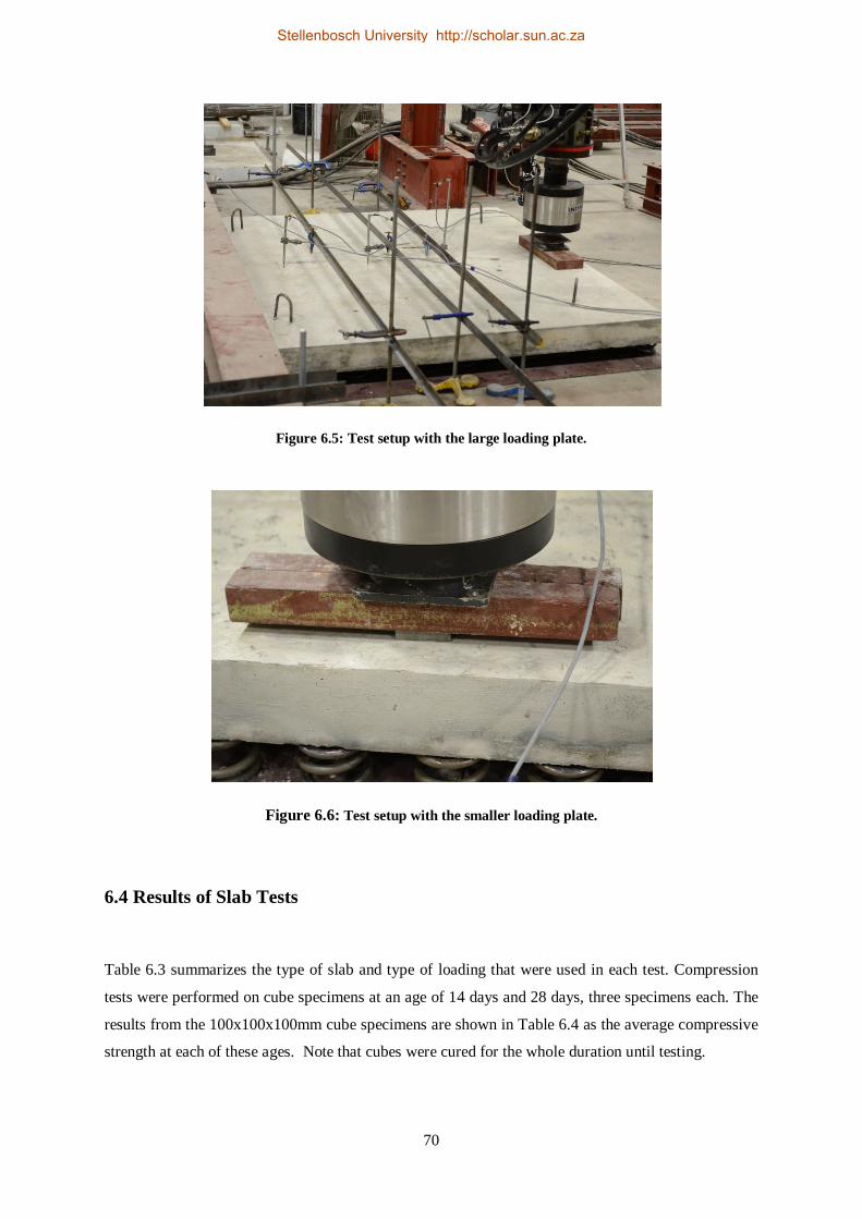
70
Figure 6.5: Test setup with the large loading plate.
Figure 6.6: Test setup with the smaller loading plate.
6.4 Results of Slab Tests
Table 6.3 summarizes the type of slab and type of loading that were used in each test. Compression
tests were performed on cube specimens at an age of 14 days and 28 days, three specimens each. The
results from the 100x100x100mm cube specimens are shown in Table 6.4 as the average compressive
strength at each of these ages. Note that cubes were cured for the whole duration until testing.
Stellenbosch University http://scholar.sun.ac.za

71
Table 6.3: Summary of tests indicating the type of slab and loading area.
Fibres Loading Area
Test 1 No Large Test 2 Yes Large Test 3 Yes Small Test 4 No Small
Table 6.4: Compressive strength of the concrete used in slab tests.
Test 1 Test 2 Test 3 Test 4
Plain
Concrete SynFRC SynFRC Plain Concrete
14 day Strength (MPa) 27 23 25 25
28 day Strength (MPa) 35 31 29 29
The slabs were tested on an age of 28 days after being cured for 14 days. This is typically the
duration of curing in practice. The aim was however to test the slabs at an age of 14 days, but due to
unforeseen circumstances this was not possible. As the curing was done for 14 days it is believed that
the 28 day behaviour is similar to the 14 day behaviour. The results given in this chapter gives the
data obtained from the tests by showing the maximum load, deflection of the slabs, and the yield-line
patterns observed. In Chapter 7 this data is analysed to give the corresponding moments that were
reached during the tests. Table 6.5 gives the values of maximum displacement and loads reached
during the tests. Each test is discussed separately in the following sections.
Table 6.5: Results from large scale slab tests.
Test Nr. Type Load area
(mm²) Ultimate Load
(kN) Load at first visible
crack (kN) Deflection at loading (mm)
Test 1 Plain Concrete 60750 71.52 71.52 12.49
Test 2 SynFRC 60750 105.78 77.28 24.57 Test 3 SynFRC 4675 61.7 55.94 25
Test 4 Plain Concrete 4675 44.78 36.94 10.47
Stellenbosch University http://scholar.sun.ac.za
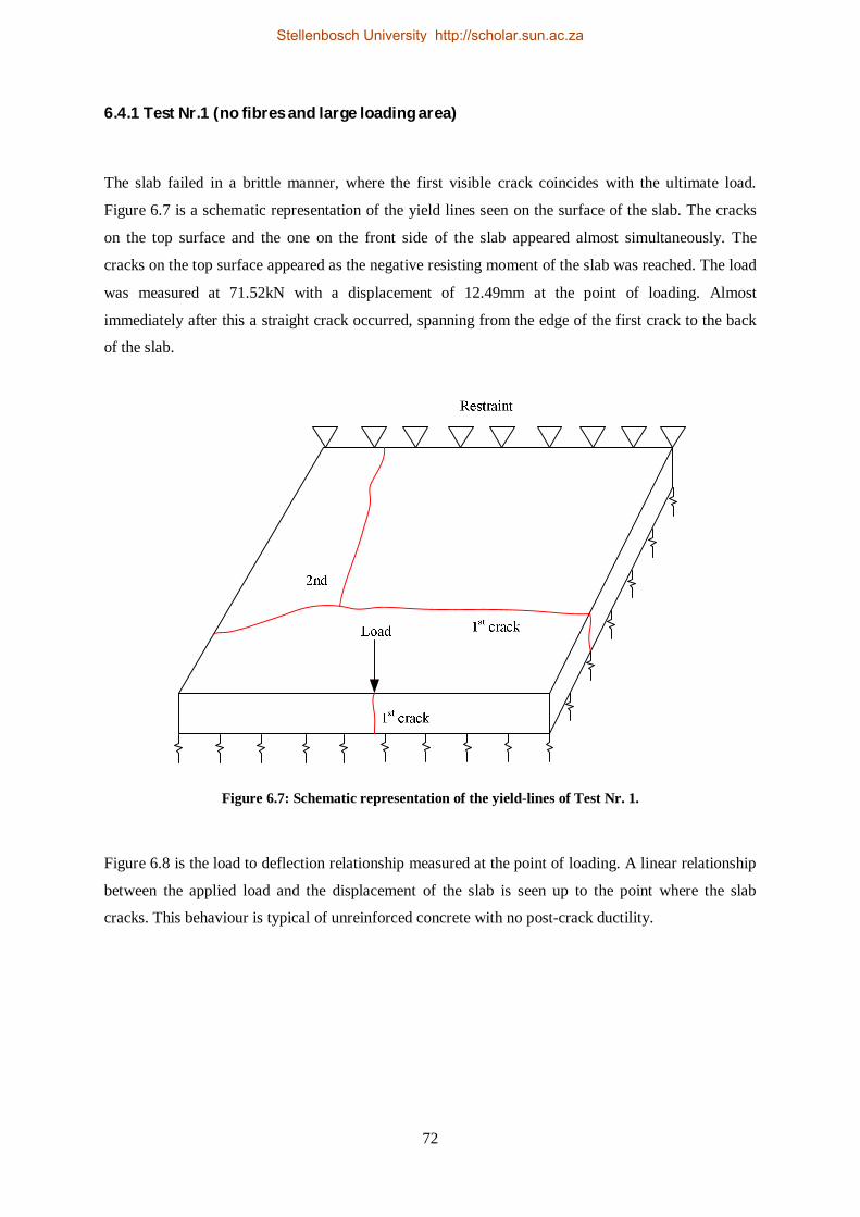
72
6.4.1 Test Nr.1 (no fibres and large loading area)
The slab failed in a brittle manner, where the first visible crack coincides with the ultimate load.
Figure 6.7 is a schematic representation of the yield lines seen on the surface of the slab. The cracks
on the top surface and the one on the front side of the slab appeared almost simultaneously. The
cracks on the top surface appeared as the negative resisting moment of the slab was reached. The load
was measured at 71.52kN with a displacement of 12.49mm at the point of loading. Almost
immediately after this a straight crack occurred, spanning from the edge of the first crack to the back
of the slab.
Figure 6.7: Schematic representation of the yield-lines of Test Nr. 1.
Figure 6.8 is the load to deflection relationship measured at the point of loading. A linear relationship
between the applied load and the displacement of the slab is seen up to the point where the slab
cracks. This behaviour is typical of unreinforced concrete with no post-crack ductility.
Stellenbosch University http://scholar.sun.ac.za

73
Figure 6.8: Load to deflection curve of Test Nr. 1.
The displacements that were measured on the centreline of the slab as the load was increased are
shown in Figure 6.9. This figure shows the deformation of the slab at the points where measurements
was taken.
Figure 6.9: Deformation of the slab from Test Nr. 1 across its centreline with an increase in load.
At a distance of approximately 1100mm from the front edge of the slab, a hinge formed. This
assumption can be made as this is a local point where no displacement was measured. This is the
position on the slab which corresponds to the first crack seen on the surface which propagated across
the slab.
0
10
20
30
40
50
60
70
80
0 2 4 6 8 10 12 14
Load
(kN
)
Deflection at point of loading (mm)
-14-12-10
-8-6-4-202
0 200 400 600 800 1000 1200 1400 1600 1800 2000
Ver
tica
l dis
plac
emen
t (m
m)
Distance along centreline of specimen (mm)
0 kN 14.3 kN 28.62 kN 42.9 kN 57.2 kN 71.52 kN
Hinge Restraint
Stellenbosch University http://scholar.sun.ac.za

74
6.4.2 Test Nr. 2 (fibres and large loading area)
The behaviour of this slab was similar to the first slab by also following an initial linear response in
terms of load to displacement. However, after the first visible cracks started forming on the top
surface of the slab, plastic behaviour was observed. The initial cracks formed at a load of 77.28kN
with a corresponding displacement of 12.62mm and a sudden decrease in load followed. The crack
had a circular form across the top surface of the slab and propagated from the top surface downwards
through the edges of the slab as shown in Figure 6.10. A crack also appeared on the front side of the
slab where load was applied which started to propagate from the bottom surface across the depth of
the slab. This is due to a positive bending moment exceeding the resistance of the concrete. This value
for load is similar to the first-crack load of the plain concrete slab of Test Nr. 1. The load was
increased as the displacement increased and a deflection hardening behaviour was witnessed as the
fibres bridged the initial cracks. Another major circular crack formed inside the perimeter of the first
one at a load of 101.76kN at a corresponding displacement of 19.95mm. This crack propagated
through the depth of the slab at the edge where load was applied. This is an example of a term called
multiple cracking which coincides with hardening behaviour. Three vertical cracks formed on the
front edge and were caused by a positive bending moment as seen on Figure 6.10 (3rd crack). The
ultimate load that was reached during the test was 105.78kN at a deflection of 24.57mm. The
behaviour of the slab as described can be seen in Figure 6.11 which shows the load to deflection
diagram recorded at the point where the load was applied.
Figure 6.10: Schematic representation of the yield-lines on Test Nr. 2.
Stellenbosch University http://scholar.sun.ac.za

75
Figure 6.11: Load to deflection behaviour of Test Nr. 2.
Figure 6.12 shows the deformation measured at the centreline of the slab to represent the profile of the
deformed slab. The deformation of the slab is different from the one of Test Nr. 1 with a hinge
forming between 1.5m and 1.6m from the loaded edge. This corresponds to the location of the first
crack on the top surface caused by the hogging moment. The curve representing the displacements at
the ultimate load (105.78kN) shows the point at which the second circular crack appeared on the
surface at a distance of 800mm from the loaded edge.
Figure 6.12: Deformation of the slab from Test Nr. 2 across its centreline with an increase in load.
0
20
40
60
80
100
120
0 5 10 15 20 25 30
Load
(kN
)
Deflection at point of loading (mm)
-30
-25
-20
-15
-10
-5
0
5
0 200 400 600 800 1000 1200 1400 1600 1800 2000
Ver
tica
l dis
plac
emen
t (m
m)
Distance along centreline of specimen (mm)
0 kN 21.16 kN 42.3 kN 63.46 kN 84.62 kN 105.78 kN
2nd hinge
1st hinge Restraint
1st crack
2nd crack 3rd crack
Stellenbosch University http://scholar.sun.ac.za

76
6.4.3 Test Nr.3 (fibres and small loading area)
This was the first slab tested with the smaller loading plate (100x50x20mm). The purpose was
initially to test for punching shear, but due to the continuous support provided by the bed of springs,
the mode of failure was of a flexural nature. The slab’s response differed from the previous two tests
by failing under the positive bending moment first. This can be said since the first visible crack
formed on the bottom of the slab and propagated through the depth of the slab on the front edge. The
crack occurred at a load of 55.94kN and a displacement of 10.41mm. The second crack formed on the
top surface, circular in shape and spanned across the width of the slab cutting through the edges. This
crack formed at a load of 56.44kN and a displacement of 14.71mm. The second and third circular
crack on the top surface occurred without any significant decrease in force. Near the end of the test, a
straight line crack formed on the top surface which propagated from the centre of the first circular
crack and stopped before reaching the back edge. The maximum load measured during the test was
61.7kN at a displacement of 25mm. Figure 6.13 shows the yield-lines and the order in which they
occurred.
1st
2nd
3rd
4th
5th
Load
Restraint
Figure 6.13: Schematic representation of the yield lines on Test Nr. 3.
The load to deflection curve of Figure 6.14 shows the initial linear elastic response of the slab
followed by a smooth curve representing the plastic behaviour of the slab after the first crack
occurred.
Stellenbosch University http://scholar.sun.ac.za
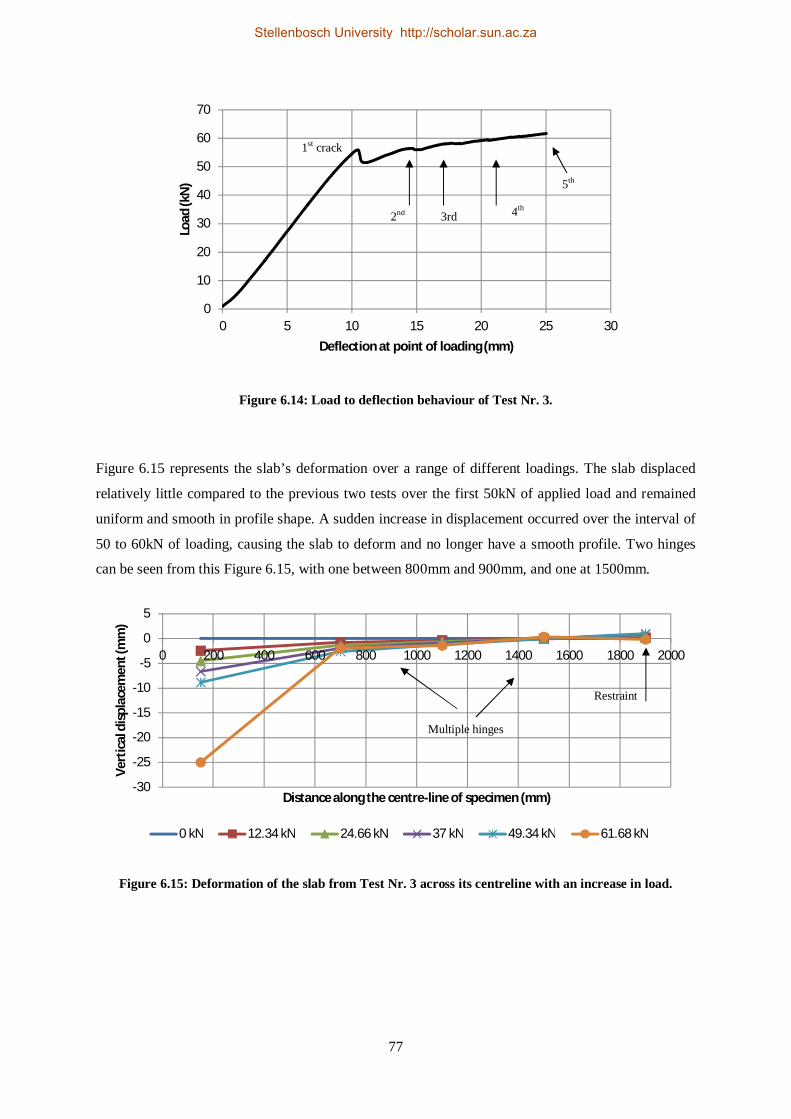
77
Figure 6.14: Load to deflection behaviour of Test Nr. 3.
Figure 6.15 represents the slab’s deformation over a range of different loadings. The slab displaced
relatively little compared to the previous two tests over the first 50kN of applied load and remained
uniform and smooth in profile shape. A sudden increase in displacement occurred over the interval of
50 to 60kN of loading, causing the slab to deform and no longer have a smooth profile. Two hinges
can be seen from this Figure 6.15, with one between 800mm and 900mm, and one at 1500mm.
Figure 6.15: Deformation of the slab from Test Nr. 3 across its centreline with an increase in load.
0
10
20
30
40
50
60
70
0 5 10 15 20 25 30
Load
(kN
)
Deflection at point of loading (mm)
-30
-25
-20
-15
-10
-5
0
5
0 200 400 600 800 1000 1200 1400 1600 1800 2000
Ver
tica
l dis
plac
emen
t (m
m)
Distance along the centre-line of specimen (mm)
0 kN 12.34 kN 24.66 kN 37 kN 49.34 kN 61.68 kN
1st crack
2nd 3rd 4th
5th
Multiple hinges
Restraint
Stellenbosch University http://scholar.sun.ac.za
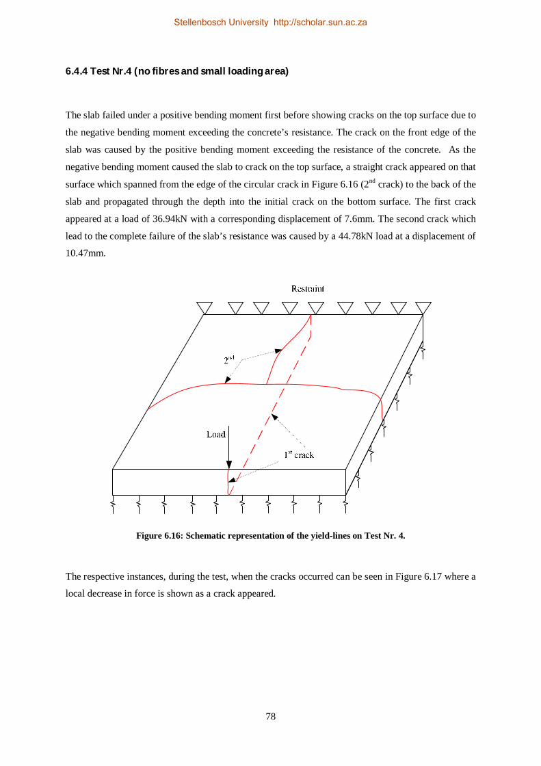
78
6.4.4 Test Nr.4 (no fibres and small loading area)
The slab failed under a positive bending moment first before showing cracks on the top surface due to
the negative bending moment exceeding the concrete’s resistance. The crack on the front edge of the
slab was caused by the positive bending moment exceeding the resistance of the concrete. As the
negative bending moment caused the slab to crack on the top surface, a straight crack appeared on that
surface which spanned from the edge of the circular crack in Figure 6.16 (2nd crack) to the back of the
slab and propagated through the depth into the initial crack on the bottom surface. The first crack
appeared at a load of 36.94kN with a corresponding displacement of 7.6mm. The second crack which
lead to the complete failure of the slab’s resistance was caused by a 44.78kN load at a displacement of
10.47mm.
Figure 6.16: Schematic representation of the yield-lines on Test Nr. 4.
The respective instances, during the test, when the cracks occurred can be seen in Figure 6.17 where a
local decrease in force is shown as a crack appeared.
Stellenbosch University http://scholar.sun.ac.za

79
Figure 6.17: Load to deflection behaviour of Test Nr. 4.
The deformation of the slab, as measured on its centreline, was similar to that of the Test Nr. 1.
Complete failure can be seen from the graph representing the slab’s response to the load of 44.78kN
in Figure 6.18.
Figure 6.18: Deformation of the slab from Test Nr. 4 across its centreline with an increase in load.
6.5 Discussion on Results of Slab Tests
The overall performance of the fibre reinforced slabs showed a substantial increase in ductility
compared to the plain concrete. In the first two tests, with the large loading plate (Test Nr. 1 and
Nr. 2), the first cracks appeared at 71.52kN and 77.28kN for the plain concrete and SynFRC
respectively. The higher value measured for the SynFRC is due effect of the fibres, which explain the
increased modulus of rupture of the SynFRC slab. The second crack that formed on the top surface
(small circular crack in Figure 6.10) was caused as the induced negative moment exceeded the
0
10
20
30
40
50
0 2 4 6 8 10 12
Load
(kN
)
Deflection at the point of loading (mm)
-12
-10
-8
-6
-4
-2
0
2
4
0 500 1000 1500 2000
Ver
tica
l dis
plac
emen
t (m
m)
Distance along the centre-line of specimen (mm)
0 kN 8.96 kN 17.9 kN 26.88 kN 35.82 kN 44.78 kN
1st crack 2nd
Hinge from hogging moment
Restraint
Stellenbosch University http://scholar.sun.ac.za

80
resistance capacity of the concrete at that point. It could be explained that the slab formed another
hinge as the fibres bridging the first crack on the surface of the slab caused the negative bending
moment to increase, thus inducing larger negative moments across the length of the slab. Although
cracks occurred on the slab’s surfaces, it was still structurally sound after initial cracking, showing a
deflection hardening behaviour on the spring support. The test was concluded at a displacement of
25mm for the SynFRC slab because of the springs being fully compressed at that point.
The tests performed with the smaller loading plate (Test Nr. 3 and Nr. 4) showed somewhat different
behaviour under loading. Although the exact same test setup was used for all the tests, the specific
mode of failure for the initial cracks was different in Test Nr. 3 and Test Nr. 4. Where the slabs from
Test Nr. 1 and Nr. 2 failed under an induced hogging moment first, these slabs failed under a sagging
moment first. The larger loading plate, with a width of 450mm, effectively caused the slab to span in
the direction of the restraint. The applied load then caused a negative bending moment over the span
length which leads to failure as the concrete’s capacity was exceeded. By using the smaller loading
plate (100x50mm) with the shorter side parallel to the restraint, the slab’s principle direction of span
could become perpendicular to the restraint as shown in Figure 6.19.
Figure 6.19: Slab span direction for large- and small load plates.
In the tests with the small load plate a positive bending moment was induced at the centre of the slab
which leads to a crack forming and propagating from the bottom towards the top surface on the
centreline of the slab. After this first mode of bending failure, the other direction of span became the
principle one, leading to failure under a negative moment.
Stellenbosch University http://scholar.sun.ac.za

81
The elastic sections of the curves showing the load to deflection behaviour of the slabs for Test Nr. 3
and Test Nr. 4 are similar in shape and in gradient. The load at which the SynFRC slab first cracked
under the induced sagging moment is higher than the one causing the plain concrete to fail (55.94kN
compared to 36.94kN). This can be explained as the fibres having an effect on the behaviour of the
concrete. The first “jump” in the load-deflection curve of Test Nr. 4 (Figure 6.17) shows the point at
which the concrete’s sagging moment resistance was reached. The second “jump” indicates the point
where the concrete’s hogging moment resistance was reached as the direction of span changed.
The deflection hardening behaviour from the SynFRC slabs proves that the addition of synthetic
fibres increases the ductility of the concrete. The ultimate load reached during Test Nr.2 was
105.78kN compared to 71.52kN from Test Nr. 1. Although the slab from Test Nr.4 reached a higher
load after the first crack occurred, this load is not seen as the ultimate load since this slab was
unreinforced and lost all structural integrity after the first crack occurred. The ultimate load from Test
Nr. 3 was 61.7kN compared to the plain concrete slab of Test Nr. 4 with an ultimate load of 44.78kN.
Large deflections were measured at higher loads, which is undesirable from a serviceability point of
view. The advantage from a structural point of view is that when the elastic design load of a slab was
reached due to an unforeseen event, sudden brittle failure can be prevented by using fibres. The slab
will remain structurally sound if the applied load did not cause ultimate failure such as fibre rupture
and the cracks can be repaired.
6.6 Concluding Summary
The addition of 6kg/m3 of fibres increased the concrete slabs’ first cracking strength as well as post-
crack ductility compared to the plain concrete slabs. The slabs reinforced with fibres achieved higher
loads after first cracks occurred, while the maximum load that the plain concrete slabs could resist is
the first cracking load. The fibres provided ductility when it bridged larger crack widths and this lead
to higher post first-crack loads.
Stellenbosch University http://scholar.sun.ac.za
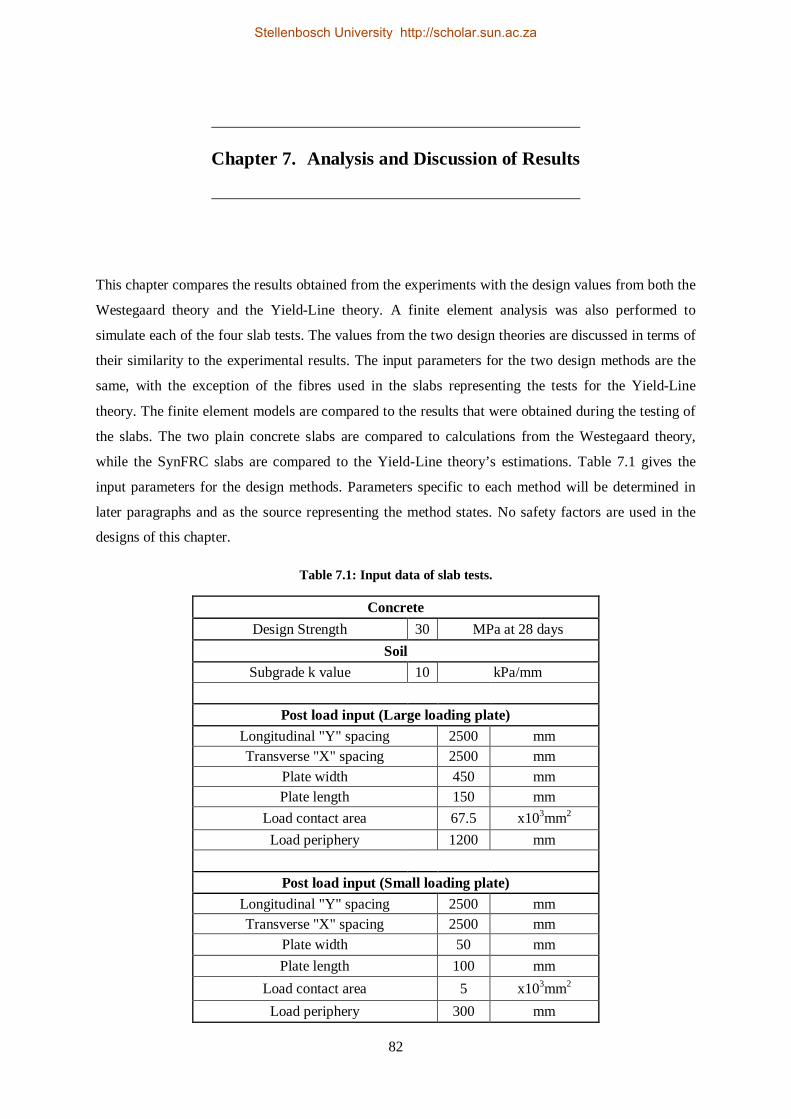
82
This chapter compares the results obtained from the experiments with the design values from both the
Westegaard theory and the Yield-Line theory. A finite element analysis was also performed to
simulate each of the four slab tests. The values from the two design theories are discussed in terms of
their similarity to the experimental results. The input parameters for the two design methods are the
same, with the exception of the fibres used in the slabs representing the tests for the Yield-Line
theory. The finite element models are compared to the results that were obtained during the testing of
the slabs. The two plain concrete slabs are compared to calculations from the Westegaard theory,
while the SynFRC slabs are compared to the Yield-Line theory’s estimations. Table 7.1 gives the
input parameters for the design methods. Parameters specific to each method will be determined in
later paragraphs and as the source representing the method states. No safety factors are used in the
designs of this chapter.
Table 7.1: Input data of slab tests.
Concrete Design Strength 30 MPa at 28 days
Soil Subgrade k value 10 kPa/mm
Post load input (Large loading plate)
Longitudinal "Y" spacing 2500 mm Transverse "X" spacing 2500 mm
Plate width 450 mm Plate length 150 mm
Load contact area 67.5 x103mm2 Load periphery 1200 mm
Post load input (Small loading plate)
Longitudinal "Y" spacing 2500 mm Transverse "X" spacing 2500 mm
Plate width 50 mm Plate length 100 mm
Load contact area 5 x103mm2 Load periphery 300 mm
Chapter 7. Analysis and Discussion of Results
Stellenbosch University http://scholar.sun.ac.za

83
7.1 Design Using the Westegaard Theory
All equations used are from Concrete Industrial Floors on the Ground by Marais and Perrie
(1993).The flexural strength of the concrete can be determined by using Equation 4.1.
The flexural strength for concrete used in the two plain slabs was determined from Eq. 4.1 as 3.8MPa
by using an average strength of 38MPa for the 30MPa (design strength) concrete mix (Marais &
Perrie, 1993).
The three graphs given for the design of point loads are for subgrade k-values of 15-, 30- and
55kPa/mm respectively. The stiffness provided by the spring support was determined as 10kPa/mm.
To obtain the predicted point load capacity, the values obtained from the three curves were
extrapolated to a value of 10kPa/mm of soil support (Figures A1, A2 and A3 in Addendum A).
The longitudinal and lateral spacing of the posts were chosen as 2500mm and 2500mm respectively
since these are the largest spacing for which the design curves from Concrete Industrial Floors on the
Ground by Marais and Perrie (1993) can be used. These spacings were chosen to isolate the effect of
other posts loads.
7.1.1 Design Load for Large Load Plate
The load area is large enough not to need Figure 4.3 to obtain an effective load contact area.
Figure A1 is entered from the top left corner with a slab depth of 120mm. The intersection with the
“X”- spacing is marked and then move to the right towards the intersection with the “Y”-spacing. The
next move is down to a load contact area just past the 50x103 mm2 line (largest contact area on the
graphs). From this point the intersection with a concrete stress of 3.8MPa (no safety factor as
experimental conditions were maintained, point just right of the 3.0MPa line) was made and by
moving down, a post load of 44kN was obtained. This load was determined for a slab supported by a
subgrade k-value of 15kPa/mm. Similar procedures were followed to determine the predicted ultimate
post load for subgrade k-values of 30- and 55kPa/mm respectively. For a subgrade value of
30kPa/mm a load of 46kN was obtained and for a k-value of 55kPa/mm the load was 53kN. The
design curves used for these two subgrade values are found in Addendum A (Figures A2 and A3).
Figure 7.1 shows the curve used for extrapolation to get a value for the load at a k-value of
10kPa/mm. The equation of the regression line used for extrapolation is shown on the figure along
with the R2-value of 0.98. By using the equation on the graph, a load of 42.5kN was obtained.
Stellenbosch University http://scholar.sun.ac.za
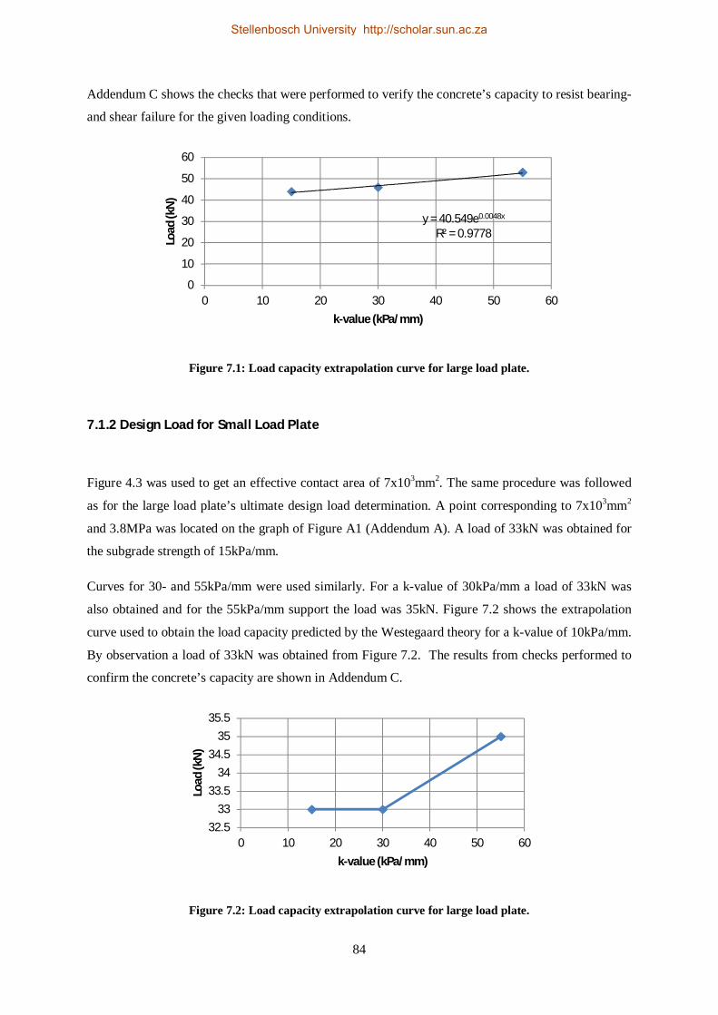
84
Addendum C shows the checks that were performed to verify the concrete’s capacity to resist bearing-
and shear failure for the given loading conditions.
Figure 7.1: Load capacity extrapolation curve for large load plate.
7.1.2 Design Load for Small Load Plate
Figure 4.3 was used to get an effective contact area of 7x103mm2. The same procedure was followed
as for the large load plate’s ultimate design load determination. A point corresponding to 7x103mm2
and 3.8MPa was located on the graph of Figure A1 (Addendum A). A load of 33kN was obtained for
the subgrade strength of 15kPa/mm.
Curves for 30- and 55kPa/mm were used similarly. For a k-value of 30kPa/mm a load of 33kN was
also obtained and for the 55kPa/mm support the load was 35kN. Figure 7.2 shows the extrapolation
curve used to obtain the load capacity predicted by the Westegaard theory for a k-value of 10kPa/mm.
By observation a load of 33kN was obtained from Figure 7.2. The results from checks performed to
confirm the concrete’s capacity are shown in Addendum C.
Figure 7.2: Load capacity extrapolation curve for large load plate.
y = 40.549e0.0048x
R² = 0.9778
0
10
20
30
40
50
60
0 10 20 30 40 50 60
Load
(kN
)
k-value (kPa/mm)
32.5
33
33.5
34
34.5
35
35.5
0 10 20 30 40 50 60
Load
(kN
)
k-value (kPa/mm)
Stellenbosch University http://scholar.sun.ac.za

85
7.2 Design Using the Yield-Line Theory
The same equations apply for determining the parameters specific to this method as in Chapter 4.
Table 7.2 shows the parameters used in determining the ultimate load capacity of the slab.
Table 7.2: Parameters used in the Yield-Line theory for the large load plate.
Description Symbol and equation Value Unit Design compressive strength of
concrete fcd 30 MPa
Radius of relative stiffness l = (Ecm h3/12(1-v2 )k)0.25 828.928 mm
Short term modulus of elasticity Ecm = 22*(fcm/10)0.3 31.475 kN/mm2
poison ratio v 0.2 Slab thickness h 120 mm
Modulus of subgrade reaction k 0.01 N/mm3 Mean compressive strength of
concrete (cylinder) fcm (from TR 34 for 30MPa fcd) 33 MPa
Characteristic flexural strength fctk,fl =(1+(200/h)0.5)*fctk(0.05) ≤ 2*fctk(0.05) 3.6 MPa Characteristic axial tensile
strength (5% fractile) fctk(0.05) (from TR 34 for 30MPa fcd) 1.8 MPa
Minimum shear strength vRd,ct =0.035*k13/2fck1/2 0.495 MPa
k1 1+(200/d)0.5 ≤ 2 2 Effective depth d = 0.75*h 90 mm
Characteristic compressive strength (cylinder) fck (from TR 34 for 30MPa fcd) 25 MPa
General Yield-Line moment capacity M = fctk,fl(h2/6) 8640 Nm/m
Ultimate negative resistance moment Mn = (fctk,fl/ λc )(h2/6) 8640 N.m/m
Ultimate positive resistance moment Mp = (fctk,fl/ λc )(Re,3)(h2/6) 4838.4 N.m/m
Partial safety factor for concrete Yc 1 Equivalent flexural strength
ratio Re,3 0.56
Equivalent contact radius a 146.581 mm
a/l = 0.177
The only parameter used from experimental data is the Re,3 value in Table 7.2 which were obtained in
Chapter 5. The other parameters were used as stipulated in Concrete Industrial Ground Floors,
Technical Report No. 34 by the Concrete Society UK (2003).
Stellenbosch University http://scholar.sun.ac.za

86
7.2.1 Design for the Large Loading Area
By using Equations 4.18 to 4.24 and the values of Table 7.2, Table 7.3 was compiled which shows the
ultimate loads that can be applied at the three areas of the slab (interpolated for a/l = 0.177).
Table 7.3: Load capacity of the SynFRC slab for a large loading plate (Yield-Line theory).
a/l a/l a/l 0 >0.2 0.177 0 >0.2 0.177 0 >0.2 0.177
Internal Load (kN) Edge Load (kN) Corner Load (kN) 84.7 180.0 168.9 38.5 87.2 81.5 17.3 42.0 39.1
The slabs were loaded on the edge region. A check could be made to confirm that the concrete’s shear
resistance will not be exceeded at this region. Table 7.4 shows such a test and gives the equations
used to determine the predicted shear capacity for loading with the large load plate. The specific
placing of the load plate on the edge of the slab is shown in Figure 7.3 as well as the perimeter of the
load.
Figure 7.3: Position and periphery of large load plate.
Table 7.4: Shear strength of concrete loaded with the large load plate (Yield-Line theory).
u0 (Perimeter at face of loaded area) 850 mm
k2 = 0.6*(1-fck/250) 0.54
Should not exceed vmax = 0.5*k2*fck/λc 6.75 MPa
At critical perimeter
u1 = u0 +π(2*d) 1415.49 mm
Pp = (0.035k13/2fck
1/2)u1d 63.06 kN
Stellenbosch University http://scholar.sun.ac.za

87
7.2.2 Design for the Small Loading Area
The calculations are similar for the slab loaded with the small loading plate. The only value that
changes in Table 7.2 is the equivalent contact radius which becomes 39.9mm with a/l = 0.0481.
The load capacities for the different regions on the slab are given in Table 7.5.
Table 7.5: Load capacity of the SynFRC slab for a small loading plate (Yield-Line theory).
a/l a/l a/l 0 >0.2 0.0481 0 >0.2 0.0481 0 >0.2 0.0481
Internal Load (kN) Edge Load (kN) Corner Load (kN) 84.7 172.1 105.7 38.5 79.5 48.3 17.3 36.3 21.9
The shear resistance of the 120mm thick slab loaded with the small loading plate is given in Table 7.6
as 49.69kN. Figure 7.4 shows the perimeter of the loaded area and the specific load plate placement.
Figure 7.4: Position and periphery of small load plate (Yield-Line theory).
Table 7.6: Shear strength of concrete loaded with the small load plate.
u0 (Perimeter at face of loaded area) 550 mm
k2 = 0.6*(1-fck/250) 0.54
Should not exceed vmax = 0.5*k2*fck/λc 6.75 MPa
At critical perimeter
u1 = u0 +π(2*d) 1115.49 mm
Pp = (0.035k13/2fck
1/2)u1d 49.69 kN
Stellenbosch University http://scholar.sun.ac.za

88
7.3 Finite Element Analysis
PROKON™, a locally available finite element software, was used to model the experimental tests on
the slabs with a numerical approach. Each of the four tests were simulated by applying the load that
lead to first crack to a mesh of shell elements representing the slab. The essential output that is of
interest is the value of the maximum induced moment as well as the predicted displacement. Only the
load at first crack can be modelled accurately with elastic theory finite element modelling (FEM). The
post first-crack behaviour enters the plastic region of material behaviour and falls outside the scope of
this chapter.
In order to simulate test conditions as accurately as possible the exact positioning of the slab relative
to the spring bed was modelled. The area of the slab that falls within the perimeter of the bed of
springs is 1950x1950mm. This part of the slab was modelled by shell elements of 50x50mm. The
slabs were placed with the loaded edge in-line with the first row of springs. This means that the slab
extended 50mm over the springs at the back, where it was restrained, and 25mm on each of the other
two sides. Part of the slab that extended at the back was also modelled with 50x50mm shell elements.
The sides where 25mm extended over the spring support were modelled as 25x50mm shells. All
shells were 120mm thick with a 30MPa concrete as material. Spring elements were used as support
over the 1950x1950mm area at 150mm centres in both directions. The H-beam that provided the
restraint, preventing the slabs from lifting up at the back, was modelled by specifying no movement in
the “Y”-direction at the nodes corresponding to that position. Figure 7.5 shows an example from one
of the models where the modelling of the springs, the shells and the restraint can be seen.
Figure 7.5: Modelling of shell elements, springs and the restraint representing the H-beam.
Stellenbosch University http://scholar.sun.ac.za

89
The load that was used in each case was applied as shell loads at the respective positions
corresponding to that of the actual tests. The load at first crack was divided by the area in contact with
the slab to get a distributed load over the shell elements at those points. Figure 7.6 shows an example
of how the loads were modelled for both the large- and small load plates.
Figure 7.6: Modelling of the large (top)- and small (bottom) load plates.
The models for the plain concrete and SynFRC slabs for the tests with the large load plate was
modelled first with the only difference between the two simulations being the load at first crack as
input. Table 7.7 gives the results from the simulations. The maximum displacement was obtained at
the centre of the slab’s edge where load was applied in both cases.
Table 7.7: Maximum induced moments around the x-axis from the FEM-models for the large load plate.
Slab type Load (kN)
Induced negative moment (kNm/m)
Induced Positive moment (kNm/m)
Max. Displacement (mm)
Plain concrete 71.52 -7.918 3.768 6.1
SynFRC 77.28 -8.584 4.067 6.56
The moments shown in Table 7.7 are the moments around the x-axis which are induced as the slabs
effectively span from the load towards the restraint. Figure 7.7 shows the distribution of moment
Stellenbosch University http://scholar.sun.ac.za

90
forces over the plain concrete (top) and the SynFRC (bottom) slabs. In each of the following figures
the largest negative moments are indicated by dark blue and the largest positive moments by red.
Figure 7.7: Distribution of the induced moments for plain concrete (top) and SynFRC (bottom) slabs (large load plate, principle span direction).
Table 7.8 shows values from the moments induced over the span in the direction perpendicular to the
principle span direction.
Stellenbosch University http://scholar.sun.ac.za

91
Table 7.8: Maximum induced moments around the y-axis from the FEM-models for the large load plate.
Slab type Load (kN)
Induced negative moment (kNm/m)
Induced Positive moment (kNm/m)
Plain concrete 71.52 -1.518 20.54
SynFRC 77.28 -1.639 22.19
Figure 7.8 shows the distribution of the moments, seen in Table 7.8, over the slabs.
Figure 7.8: Distribution of the induced moments for plain concrete (top) and SynFRC (bottom) slab (large load plate, perpendicular to principle span direction).
Table 7.9 shows the results from the models simulating the tests with the smaller load plate. Note that
the positive moments exceed the values of the negative moments at a lower applied load than in the
previous models for moments around the x-axis. Figure 7.9 shows the distribution of these moments
across the slab.
Stellenbosch University http://scholar.sun.ac.za
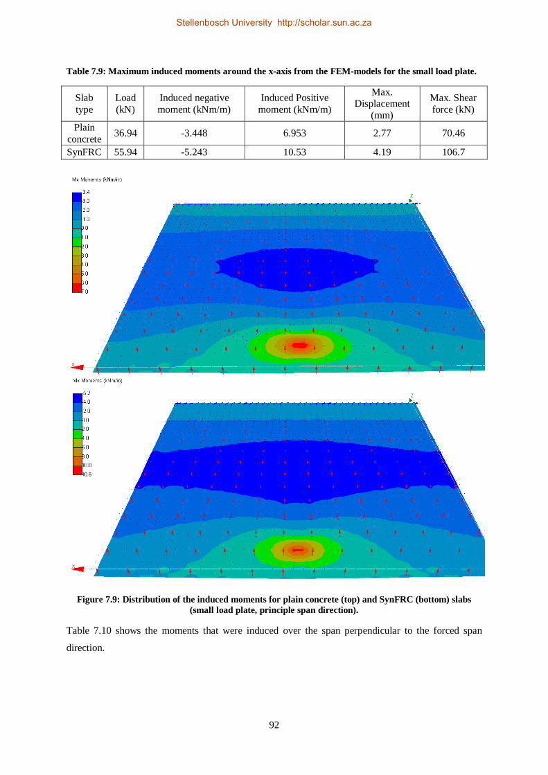
92
Table 7.9: Maximum induced moments around the x-axis from the FEM-models for the small load plate.
Slab type
Load (kN)
Induced negative moment (kNm/m)
Induced Positive moment (kNm/m)
Max. Displacement
(mm)
Max. Shear force (kN)
Plain concrete 36.94 -3.448 6.953 2.77 70.46
SynFRC 55.94 -5.243 10.53 4.19 106.7
Figure 7.9: Distribution of the induced moments for plain concrete (top) and SynFRC (bottom) slabs (small load plate, principle span direction).
Table 7.10 shows the moments that were induced over the span perpendicular to the forced span
direction.
Stellenbosch University http://scholar.sun.ac.za

93
Table 7.10: Maximum induced moments around the y-axis from the FEM-models for the small load plate.
Slab type Load (kN)
Induced negative moment (kNm/m)
Induced Positive moment (kNm/m)
Plain concrete 36.94 -0.6439 14.19
SynFRC 55.92 -0.9748 21.48
Figure 7.10 shows the distribution of the moments, seen in Table 7.10, over the slabs.
Figure 7.10: Distribution of the induced moments for plain concrete (top) and SynFRC (bottom) slabs (small load plate, perpendicular to principle span direction).
Stellenbosch University http://scholar.sun.ac.za

94
7.4 Comparison with Experimental Tests
Table 7.11 gives a summary of the results obtained in this chapter and also shows the corresponding
measured values from Chapter 6 for the loads that lead to the failure of the slabs. This table also gives
values for slabs designed with the Yield-Line theory which does not contain fibres. The failure load is
defined as the load at which first cracks occurred. This is when cracks occur in any part of the slab.
Table 7.11: Summary of results from this section compared to experimental results.
Predicted load
Westegaard Theory (kN)
Predicted load Yield-
Line Theory (kN)
Measured Load (kN)
Failure Moment
from FEM-Analysis (kNm/m)
Measured Displacement
(mm)
Displacement from FEM-
Analysis (mm)
Test Nr. 1 42.5 65.42 71.52 -7.918 12.49 6.1
Test Nr. 2 42.5 81.5 77.28 -8.584 12.612 6.56
Test Nr. 3 33 48.3 55.94 10.53 10.45 4.19
Test Nr. 4 33 38.77 36.94 6.953 7.57 2.77
Figure 7.11 shows the comparison between measured and predicted loads for the test with the large
load plate. From this figure it can be seen that the values predicted by the Yield-Line theory is in
closer correlation with measured values from the tests for the slabs containing fibres as well as those
of plain concrete.
Figure 7.11: Comparison between measured loads (bars) and predicted loads (lines) for small loading plate.
The Westegaard theory recommends an ultimate load capacity for the 120mm plain concrete slab as
42.5kN for the large load plate (67.5x103mm2) and 33kN for the smaller one (5x103mm2). The load
capacities measured during the experiments were 71.52kN (Test Nr. 1) and 36.94kN (Test Nr. 4)
respectively. The experimental results were 68% higher than the analytic value for the test with the
71.5277.28
0
20
40
60
80
100
Without fibres With fibres
Load
(kN
) 65.42
81.50 Yield-Linetheory
42.50 Westegaard
theory
Stellenbosch University http://scholar.sun.ac.za

95
large load plate and 14% higher for the one with the small load plate. This finding could mean that the
Westegaard theory, as used by Marais and Perrie (1993), gives conservative values for floor
thicknesses as the loads that are applied increases. The predicted ultimate load for the small load plate
was closer to the measured value of Test Nr. 4 of Chapter 6. The ultimate load that could be carried at
a corner region is also the most critical one according to the checks performed for shear capacity. The
slab of Test Nr. 4 did not fail under a shear load, but under a sagging moment. The shear resistance of
the slab was thus higher as predicted by the Westegaard theory. If one takes the above findings into
account, it could be said that the Westegaard theory is a conservative theory in terms of deriving a
floor thickness for a given point load. Figure 7.12 shows the comparison between measured and
predicted loads for the test with the small load plate. The Yield-Line theory predicts the failure loads
more accurately than the Westegaard theory. It should be noted that the Yield-Line theory
overestimated the failure load for the plain concrete slab. Since this theory efficiently includes
ductility, and since the load plate used could have caused some more severe shear forces than the
large load plate, the ductility of this slab was overestimated.
Figure 7.12: Comparison between measured loads (bars) and predicted loads (lines) for small loading plate.
The Yield-Line theory showed closer correlation between the measured values of the tests performed
on the two SynFRC slabs and the predicted loads from the theory. For the test with the large load
plate, a value of 81.5kN was predicted and 48.3kN for the small load plate for the slabs containing
fibres. The loads predicted for the slabs not containing fibres is also in a closer correlation with the
measured values as can be seen in Table 7.11. These loads are the ultimate predicted loads that can be
applied to an edge region of the slabs under the respective load conditions. The measured values at
first crack were 77.28kN (Test Nr. 2) and 55.94kN (Test Nr. 3) for the large and small area of loading
respectively. This means that the theory predicted a load 5.2% higher than the measured load for the
test with the large load plate and 16.5% lower for the one with the small plate. The Yield-Line theory
defines failure of the slab when cracks occur on the top surface. The load of 55.94kN lead to first
crack (bottom surface) for the small loading area, but that load was sustained by the fibres bridging
the crack for almost 4mm of vertical deflection before the crack on the top surface occurred (Figure
36.94
55.94
0
10
20
30
40
50
60
Without fibres With fibres
Load
(kN
) 38.77
48.30
33.00
Yield-Line theory
Westegaard theory
Stellenbosch University http://scholar.sun.ac.za

96
6.14). The estimation of shear resistance capacity was given as 63.06kN for the large load area and
49.69kN for the smaller one (Yield-Line theory). Since the slabs failed under bending forces, one
could argue that the lack of including the fibres effect on the shear capacity leads to a conservative
estimated shear resistance. Concrete Industrial Ground Floors, Technical Report No. 34 by the
Concrete Society UK (2003) do not recognise the effect of synthetic fibres in the calculations of shear
resistance and consequently calculates it as for plain concrete.
The correlations between measured- and derived values are closer for the loads predicted by the
Yield-Line theory than for those of the Westegaard theory. One explanation can be that the source of
literature used for the Westegaard theory incorporated safety factors in deriving charts from empirical
data since no safety factors were included in the calculations of this chapter. The Yield-Line theory
effectively includes the effect of the synthetic fibres since the loads at which failure occurred
correlates in close comparison to the ones predicted.
The FEM-analysis was performed to obtain values for the induced moments which occurred over the
slabs as the first cracks appeared. The two models simulating the large loading plate conditions
showed a maximum hogging moment of 7.9kNm/m and 8.6kNm/m for the plain concrete- and
SynFRC slabs respectively. Since the first cracks in both of these slabs occurred at the positions
where these hogging moments is found in Figure 7.7, it is believed that these moments (Mx) caused
the failure to occur. As explained in Chapter 6, the slabs tested with the large loading plate were
effectively forced to span over its length between the load and the restraint. This and the fact that the
patterns of the maximum moments fit those of the yield-lines found on the slabs provides enough
reason to accept the concrete’s hogging resistance was reached. The Yield-Line theory estimates the
hogging moment resistance of a 120mm thick slab as 8.64kNm/m which correlates well with the
values from the analysis.
For the models performed with the smaller load plate, the first interesting aspect that was found is that
the sagging moments exceeded the values of the hogging moments over the forced span direction. The
sagging moment values obtained from the analysis are 6.95kNm/m and 10.5kNm/m for the plain
concrete and SynFRC slabs respectively. The values are similar in magnitude as those of the
maximum hogging moments just discussed for the large load area. The slabs tested with the large
plate, failed under hogging moments first and the other two failed under a sagging moment first as
was witnessed during the experiments. It is believed that the values of the moments, as just shown
above, give the absolute moment resistance of the slab. The two tests performed with the small load
plate formed cracks that propagated from the edge of the loaded side towards the centre of the slab
(Figures 6.13 and 6.16). This could be due to the concrete reaching its ultimate moment resistance
under the applied load combined with the additional forces from the slab spanning in the other
direction as well. The Yield-Line theory describes failure from a point load as first cracks forming in
Stellenbosch University http://scholar.sun.ac.za

97
a radial direction on the bottom of a slab from a sagging moment and then circumferential cracks
appear (from hogging moments) on the surface which encloses the radial cracks (Figure 3.10). This
statement corresponds to the order and shapes in which the cracks formed in the tests with the small
load area.
The Mx and My-moments obtained by the analysis for the large load area are similar to those found in
the results from the analysis with the smaller load area. The results (moments and displacements)
from the models simulating the slabs correspond in their respective magnitudes although load area-
and magnitude were different. These moments and the respective combinations of the Mx- and My-
moments, give the resistance of the concrete against moment forces up to the first crack. The exact
moment experienced in the SynFRC slab as the circular crack formed on the surface in Test Nr. 3
cannot be calculated by elastic FEM-modelling. Despite this limitation it can be said that the Yield-
Line theory accurately predicted the loads that caused failure and that it includes the ductility
provided by the fibres effectively.
Displacements obtained from the FEM-models greatly differed from the ones measured during the
tests. From Table 7.11 the difference in displacements between the FEM-models and the measured
values is approximately 100% for each of the comparing values. A possible explanation is that the
measured displacements also include the compliance of the actuator’s support structure as the
deflections used were based on the internal LVDT of the actuator.
7.5 Concluding Summary
In this chapter the experimental results from Chapter 6 were compared to the values predicted by the
Westegaard theory and the Yield-Line theory for and edge load condition and a slab thickness of
120mm. The Yield-Line theory effectively includes the effect of the fibres as the values predicted by
this theory for the two SynFRC slabs compared well with the results from Test Nr. 2 and Test Nr. 3.
The Westegaard theory gives conservative values for load capacities as significantly higher loads
were reached during Test Nr. 1 and Test Nr. 4 than predicted by this theory.
Stellenbosch University http://scholar.sun.ac.za

98
This study investigated the use of synthetic fibres in the design of concrete floors on grade. The aim
of the research was to investigate two different design methods for slabs on grade for their design
accuracy in combination with the effect of fibres. The Westegaard theory, which is an elastic theory,
and the Yield-Line theory, which is a plastic theory, were used as design methods. Tests were
performed on concrete specimens to determine the flexural strength as well as ductility provided by
the addition of synthetic fibres. Large scale tests were performed on 2x2m slabs with a thickness of
120mm to verify the accuracy of the two design theories.
For the same applied loads, the Westegaard theory gives thicker design depths (22.5% more) for slabs
than the Yield-Line theory for a conceptual design of a typical industrial facility. The Westegaard
theory does not include the effect of fibres added to concrete since it defines failure when any form of
cracking occurs in a floor slab. This approach to solve a design problem with elastic theory makes the
Westegaard theory a conservative design method.
The Yield-Line theory on the other hand incorporates the ductility provided by the fibres and by using
plastic theory reduces the design depth of slabs on grade. Failure is still defined as once the first crack
on the top surface of a slab occurs, but includes the ductility gained from the fibres in reaching higher
positive moments after first cracks occurred on the bottom of a slab. The checks performed in this
theory, just as for the Westegaard theory, ensure that the slab is sufficiently thick to resist shear forces
induced by the applied loads. This makes the Yield-Line theory more effective from a design
perspective since it provides for thinner slabs while still complying with the requirements of both the
ultimate and serviceability limit states.
The literature used to represent the Yield-Line theory, Concrete Industrial Ground Floors, Technical
Report No. 34 by the Concrete Society UK (2003), states that synthetic fibres may be used in concrete
and the effect of its ductility included in design equations if such concrete has a Re,3 value of 0.3 or
higher. In this study Re,3 values of 0.5 to 0.65 was obtained by testing synthetic fibre reinforced
concrete specimens containing fibres in dosages from 5kg/m3 to 6kg/m3. This makes it possible to use
the Yield-Line theory to incorporate the post crack ductility provided by the fibres added in the above
mentioned dosages.
Chapter 8. Conclusions and Recommendations
Stellenbosch University http://scholar.sun.ac.za

99
By using 6kg/m3 of macro polypropylene fibres larger ultimate edge loads were measured on slab
specimens than for the plain concrete slabs. Yield-lines formed where the concrete reached its
ultimate hogging moment resistance on the top surface of the slabs. Two different load areas were
used during the tests. The larger load area lead to the slabs failing under a negative moment first,
while the smaller load area caused the concrete to crack as a positive moment was induced which
exceeded the concrete’s resistance.
The SynFRC slabs measured higher values compared to the conventional concrete slabs for first-crack
strength (77.28kN compared to 71.52kN for large load area and 55.94kN compared to 36.94kN for the
smaller one). The SynFRC slabs also had significant post-crack ductility (105.78kN maximum load
for large load plate and 61.7kN for smaller one) compared to the brittle failure of the plain concrete
slabs at the first crack. The addition of synthetic fibres thus leads to the increased flexural strength of
the concrete in both the elastic and plastic regions of material behavior.
When the results of the large scale slab tests were compared to predicted loads from the Westegaard
theory (for plain concrete) and the Yield-Line theory for SynFRC it was found that the Yield-Line
theory showed the best correlation between the measured and calculated results. The Westegaard
theory is more conservative in the prediction of loads for a given slab depth than the Yield-Line
theory. A reason for this may be that the method used to represent the use of the Westegaard theory
inherently includes safety factors in its thickness design and the approach does not include any
ductility of the concrete.
It was found that by using synthetic fibres in a concrete mix and applying the Yield-Line theory to
determine design thicknesses and loads, thinner slabs can be used in industrial floors than would be
the case if Westegaard’s theory was used.
In both approaches the shear resistance of the slab against the imposed load is one of the main
governing factors affecting the calculated slab depth. One shortcoming of the presented Yield-Line
theory is that it does not include the effect of the synthetic fibres in the calculations of shear
resistance. There are equations which include the effect of fibres on shear strength, but are only
applicable to steel fibres.
Recommendation: It is therefore recommended that future studies investigate the effect of synthetic
fibres on the shear strength of concrete and develop design equations to include this effect.
Stellenbosch University http://scholar.sun.ac.za

100
ACI Committee, & American Concrete Institute. (2006). Design of slabs-on-ground. American
Concrete Institute.
Alhozaimy, A. M., Soroushian, P., & Mirza, F. (1996). Mechanical properties of polypropylene fiber
reinforced concrete and the effects of pozzolanic materials. Cement and Concrete Composites, 18(2),
85-92.
Ali, F., Nadjai, A., Silcock, G., & Abu-Tair, A. (2004). Outcomes of a major research on fire
resistance of concrete columns. Fire safety journal, 39(6), 433-445.
Aly, T., Sanjayan, J. G., & Collins, F. (2008). Effect of polypropylene fibers on shrinkage and
cracking of concretes. Materials and structures, 41(10), 1741-1753.
Banthia, N. (1994). Fiber Reinforced Concrete. ACI SP-142ACI, Detroit, MI, 91-119.
Banthia, N., Al-Asaly, M., & Ma, S. (1995). Behavior of concrete slabs reinforced with fiber-
reinforced plastic grid. Journal of Materials in Civil Engineering, 7(4), 252-257.
Banthia, N., Mindess, S., Bentur, A., & Pigeon, M. (1989). Impact testing of concrete using a drop-
weight impact machine. Experimental Mechanics, 29(1), 63-69.
Barros, J. A., & Figueiras, J. A. (2001). Model for the analysis of steel fibre reinforced concrete slabs
on grade. Computers & Structures, 79(1), 97-106.
Baumann, R. A., & Weisgerber, F. E. (1983). Yield-line analysis of slabs-on-grade. Journal of
Structural Engineering, 109(7), 1553-1568.
Belletti, B., Cerioni, R., Meda, A., & Plizzari, G. (2008). Design aspects on steel fiber-reinforced
concrete pavements. Journal of materials in civil engineering, 20(9), 599-607.
Bernard, E. S. (2000). Behaviour of round steel fibre reinforced concrete panels under point loads.
Materials and Structures, 33(3), 181-188.
Brandt, A. M. (2008). Fibre reinforced cement-based (FRC) composites after over 40 years of
development in building and civil engineering. Composite Structures, 86(1), 3-9.
Chapter 9. References
Stellenbosch University http://scholar.sun.ac.za

101
Cengiz, O., & Turanli, L. (2004). Comparative evaluation of steel mesh, steel fibre and high-
performance polypropylene fibre reinforced shotcrete in panel test. Cement and concrete research,
34(8), 1357-1364.
Choi, Y., & Yuan, R. L. (2005). Experimental relationship between splitting tensile strength and
compressive strength of GFRC and PFRC. Cement and concrete research, 35(8), 1587-1591.
Concrete Society Technical Report No. 34. (2003). Concrete Industrial Ground Floors – A guide to
design and construction 3rd edition. The Concrete Society UK.
Concrete Society Technical Report No. 63. (2007). Guidance for the Use of Steel-Fibre-Reinforced
Concrete. The Concrete Society UK.
Concrete Society Technical Report No. 65. (2007). Guidance on the use of Macro-synthetic-fibre-
reinforced Concrete. The Concrete Society UK.
Ding, Y., & Kusterle, W. (1999). Comparative study of steel fibre-reinforced concrete and steel mesh-
reinforced concrete at early ages in panel tests. Cement and concrete research, 29(11), 1827-1834.
Elsaigh, W. A., Kearsley, E. P., & Robberts, J. M. (2005). Steel fiber reinforced concrete for road
pavement applications. In Proceedings of the 24th Southern African Transport Conference (191-201).
Hannant, D. J. (1998). Durability of polypropylene fibers in portland cement-based composites:
eighteen years of data. Cement and concrete research, 28(12), 1809-1817.
Kayali, O., Haque, M. N., & Zhu, B. (2003). Some characteristics of high strength fiber reinforced
lightweight aggregate concrete. Cement and Concrete Composites, 25(2), 207-213.
Knapton, J. (2005). Design of Ground Bearing Concrete Slabs. African Concrete Code Symposium-
2005. John Knapton Consulting Engineers, UK. Kodur, V. K. R., Cheng, F. P., Wang, T. C., & Sultan, M. A. (2003). Effect of strength and fiber
reinforcement on fire resistance of high-strength concrete columns. Journal of Structural Engineering,
129(2), 253-259.
Labib, W., & Eden, N. (2006). An Investigation Into the Use of fibres in concrete industrial ground-
floor slabs. Liverpool John Moores University, Liverpool.
Li, V. C. (2002). Large volume, high‐performance applications of fibers in civil engineering. Journal
of Applied Polymer Science, 83(3), 660-686.
Marais, R. Pierre, D. (1993). Concrete Industrial Floors on the Ground. Portland Cement Institute.
Midrand, South Africa.
Stellenbosch University http://scholar.sun.ac.za

102
Mindess, S., & Vondran, G. (1988). Properties of concrete reinforced with fibrillated polypropylene
fibres under impact loading. Cement and Concrete Research, 18(1), 109-115.
Manolis, G. D., Gareis, P. J., Tsonos, A. D., & Neal, J. A. (1997). Dynamic properties of
polypropylene fiber-reinforced concrete slabs. Cement and Concrete Composites, 19(4), 341-349.
Owens, G. (2009). Fulton’s concrete technology. Cement and concrete institute. South Africa.
Pelisser, F., Neto, A. B. D. S. S., Rovere, H. L. L., & Pinto, R. C. D. A. (2010). Effect of the addition
of synthetic fibers to concrete thin slabs on plastic shrinkage cracking. Construction and Building
Materials, 24(11), 2171-2176.
SANS 5863:2006. (2006) Concrete tests – Compressive strength of hardened concrete. Edition 2.1
Pretoria, Standards South African.
Shah, S. P., & DIRECTOR, G. (1971). Fiber reinforced concretes. A review of capabilities.
Publication C, 810261.
Sorelli, L. G., Meda, A., & Plizzari, G. A. (2006). Steel fiber concrete slabs on ground: a structural
matter. ACI structural journal, 103(4), 551.
Soutsos, M. N., Le, T. T., & Lampropoulos, A. P. (2012). Flexural performance of fibre reinforced
concrete made with steel and synthetic fibres. Construction and Building Materials, 36, 704-710.
Tiberti, G., Plizzari, G. A., Walraven, J. C., & Blom, C. B. M. (2008). Concrete tunnel segments with
combined traditional and fiber reinforcement. In Proceedings of the fib 2008 symposium, Tailor Made
Concrete Structures, Amsterdam (199-205).
Wang, N., Mindess, S., & Ko, K. (1996). Fibre reinforced concrete beams under impact loading.
Cement and concrete research, 26(3), 363-376.
Won, J. P., Park, C. G., Lee, S. W., Jang, C. I., & Won, C. (2008). Effect of crimped synthetic fibre
surface treatments on plastic shrinkage cracking of cement-based composites. Magazine of Concrete
Research, 60(6), 421-427.
Won, J. P., Park, C. G., Lee, S. W., Jang, C. I., & Kim, H. Y. (2009). Performance of synthetic
macrofibres in reinforced concrete for tunnel linings. Magazine of Concrete Research, 61(3), 165-
172.
Zhang, M. H., Sharif, M. S. H., & Lu, G. (2007). Impact resistance of high-strength fibre-reinforced
concrete. Magazine of Concrete research, 59(3), 199-210.
Stellenbosch University http://scholar.sun.ac.za

103
Zheng, Z., & Feldman, D. (1995). Synthetic fibre-reinforced concrete. Progress in Polymer Science,
20(2), 185-210.
Zollo, R. F. (1984). Collated fibrillated polypropylene fibers in FRC. ACI Special Publication, 81.
Zollo, R. F. (1997). Fiber-reinforced concrete: an overview after 30 years of development. Cement
and Concrete Composites, 19(2), 107-122.
Stellenbosch University http://scholar.sun.ac.za

Addendum A
Stellenbosch University http://scholar.sun.ac.za

Figure A1: Post load k-15kPa/mm Design Chart (Marais & Perrie, 1993).
Stellenbosch University http://scholar.sun.ac.za

Figure A2: Post load k-30kPa/mm Design Chart (Marais & Perrie, 1993).
Stellenbosch University http://scholar.sun.ac.za
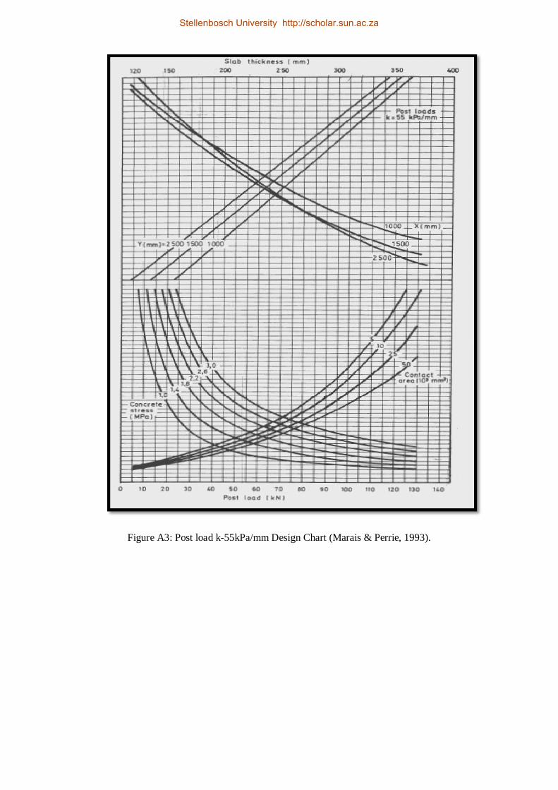
Figure A3: Post load k-55kPa/mm Design Chart (Marais & Perrie, 1993).
Stellenbosch University http://scholar.sun.ac.za

Figure A4: Wheel loads design chart: Single-Wheel -Axle Loads (Marais & Perrie, 1993).
Stellenbosch University http://scholar.sun.ac.za

Figure A5: Wheel loads design chart: Dual-Wheel -Axle Loads (Marais & Perrie, 1993).
Stellenbosch University http://scholar.sun.ac.za

Table A1: Allowable loads (kPa) for storage layout which could vary over design life (Marais &Perrie,
1993).
Stellenbosch University http://scholar.sun.ac.za

Table A2: Allowable loads (kPa) for storage layout which are fixed the over design life (Marais
&Perrie, 1993) (k =20kPa/mm).
Stellenbosch University http://scholar.sun.ac.za
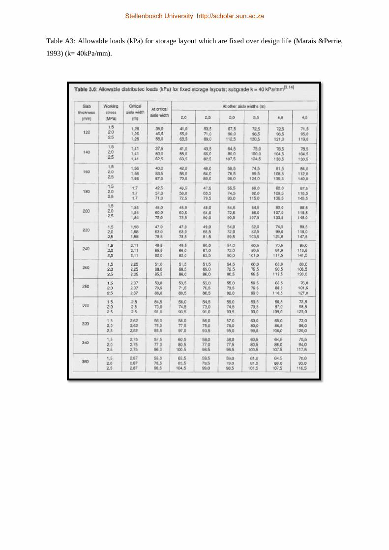
Table A3: Allowable loads (kPa) for storage layout which are fixed over design life (Marais &Perrie,
1993) (k= 40kPa/mm).
Stellenbosch University http://scholar.sun.ac.za

Table A4: Allowable loads (kPa) for storage layout which are fixed over design life (Marais &Perrie,
1993) (k= 60kPa/mm).
Stellenbosch University http://scholar.sun.ac.za

Addendum B
Stellenbosch University http://scholar.sun.ac.za

Design with the Westegaard theory.
Table B1: 40kN post load
Design steps
1. Assume safety factor (SF)
(SF = 2.0 is recommended)
2
2. Enter figure 3.6-3.8 with post load value
3. Move up to maximum concrete stress of ==> 2 MPa
4. Move right to computed contact area
5. Move up to Y spacing
6. Move left to X spacing
7. move up to slab thickness 175 mm
8.Check bearing resistance
Allowable stress Interior 4.2*ff 16.8 MPa
Edge or corner 2.1*ff 8.4 MPa
Computed stress (post load)/(load contact
area)
0.797194 MPa
OK
9.Check shear stress
Allowable shear stress 0.27*ff 1.08 MPa
computed stress
Interior
(post load)/(slab depth[(load periphery) +
4(slab depth)]
0.143215 MPa
OK
Edge
(post load)/(slab depth[0.75*(load
poeriphery) + 2*(slab depth)]
0.223651 MPa
OK
Corner
(Post load)/(slab depth*[0.5*(load
periphery) + (slab depth)]
0.366888 MPa
OK
Slab depth = 175 mm
Stellenbosch University http://scholar.sun.ac.za

Figure B1: 40kN-load Design Chart (Marais & Perrie, 1993).
Stellenbosch University http://scholar.sun.ac.za

Table B2: 50kN post load
Design steps
1. Assume safety factor (SF)
(SF = 2.0 is recommended)
2
2. Enter figure 3.6-3.8 with post load value
3. Move up to maximum concrete stress of ==> 2 MPa
4. Move right to computed contact area
5. Move up to Y spacing
6. Move left to X spacing
7. move up to slab thickness 185 mm
8.Check bearing resistance
Allowable stress Interior 4.2*ff 16.8 MPa
Edge or corner 2.1*ff 8.4 MPa
Computed stress (post load)/(load contact
area)
0.996492 MPa
OK
9.Check shear stress
Allowable shear stress 0.27*ff 1.08 MPa
computed stress
Interior
(post load)/(slab depth[(load periphery) +
4(slab depth)]
0.165202 MPa
OK
Edge
(post load)/(slab depth[0.75*(load
poeriphery) + 2*(slab depth)]
0.259376 MPa
OK
Corner
(Post load)/(slab depth*[0.5*(load
periphery) + (slab depth)]
0.426967 MPa
OK
Slab depth = 185 mm
Stellenbosch University http://scholar.sun.ac.za

Figure B2: 50kN Design Chart (Marais & Perrie, 1993).
Stellenbosch University http://scholar.sun.ac.za

Table B3: 60kN post load
Design steps
1. Assume safety factor (SF)
(SF = 2.0 is recommended)
2
2. Enter figure 3.6-3.8 with post load value
3. Move up to maximum concrete stress of ==> 2 MPa
4. Move right to computed contact area
5. Move up to Y spacing
6. Move left to X spacing
7. move up to slab thickness 195 mm
8.Check bearing resistance
Allowable stress Interior 4.2*ff 16.8 MPa
Edge or corner 2.1*ff 8.4 MPa
Computed stress (post load)/(load contact
area)
1.195791 MPa
OK
9.Check shear stress
Allowable shear stress 0.27*ff 1.08 MPa
computed stress
Interior
(post load)/(slab depth[(load periphery) +
4(slab depth)]
0.183587 MPa
OK
Edge
(post load)/(slab depth[0.75*(load
poeriphery) + 2*(slab depth)]
0.289729 MPa
OK
Corner
(Post load)/(slab depth*[0.5*(load
periphery) + (slab depth)]
0.478526 MPa
OK
Slab depth = 195 mm
Stellenbosch University http://scholar.sun.ac.za

Figure B3: 60kN Design Chart (Marais & Perrie, 1993).
Stellenbosch University http://scholar.sun.ac.za

Design with the Yield-Line theory.
40kN Post load
Table B4: Parameters for Re,3 = 0; h =125mm
Description Symbol and equation Value Unit Design compressive strength of
concrete fcd 16.67 MPa
Radius of relative stiffness l = (Ecm h3/12(1-v2 )k)0.25 649.43 mm
Short term modulus of elasticity Ecm = 22*(fcm/10)0.3 31.48 kN/mm2
poison ratio v 0.20
Slab thickness h 125.00 mm
Modulus of subgrade reaction k 0.03 N/mm3
Mean compressive strength of concrete (cylinder)
fcm (from TR 34 for 30MPa fcd) 33.00 MPa
Characteristic flexural strength fctk,fl =(1+(200/h)0.5)*fctk(0.05) ≤
2*fctk(0.05) 3.60 MPa
Characteristic axial tensile strength (5% fractile)
fctk(0.05) (from TR 34 for 30MPa fcd) 1.80 MPa
Minimum shear strength vRd,ct =0.035*k13/2fck1/2 0.49 MPa
k1 1+(200/d)0.5 ≤ 2 2.00
Effective depth d = 0.75*h 93.75 mm Characteristic compressive strength
(cylinder) fck (from TR 34 for 30MPa fcd) 25.00 MPa
General Yield-Line moment capacity M = fctk,fl(h2/6) 9375.00 kN.m
Ultimate collapse load Pu 48.00 kN
Ultimate negative resistance moment Mn = (fctk,fl/ λc )(h2/6) 6250.00 N.m
Ultimate positive resistance moment Mp = (fctk,fl/ λc )(Re,3)(h2/6) 0.00 N.m
Partial safety factor for concrete Yc 1.50
Equivalent flexural strength ratio Re,3 0.00
Equivalent contact radius a 126.38 mm
a/l = 0.196
Table B5: Ultimate load capacities for Re,3 = 0.
a/l a/l a/l 0 >0.2 0.196 0 >0.2 0.196 0 >0.2 0.196
Internal Load (kN) Edge Load (kN) Corner Load (kN)
39.3 78.5 77.5 22.3 44.6 44.0 12.5 25.0 24.7
Stellenbosch University http://scholar.sun.ac.za

Table B6: Shear capacities for Re,3 = 0.
u0 (Perimeter at face of loaded area) 672 mm
k2 = 0.6*(1-fck/250) 0.54
Should not exceed vmax = 0.5*k2*fck/λc 4.5 MPa
At critical perimeter
u1 = u0 +π(2*d) 1261.048623 mm
Pp = (0.035k13/2fck
1/2)u1d 58.51755213 kN
Table B7: Parameters for Re,3 = 0.2; h=120mm.
Description Symbol and equation Value Unit Design compressive strength of
concrete fcd 16.67 MPa
Radius of relative stiffness l = (Ecm h3/12(1-v2 )k)0.25 629.85 mm
Short term modulus of elasticity Ecm = 22*(fcm/10)0.3 31.48 kN/mm2
poison ratio v 0.20
Slab thickness h 120.00 mm
Modulus of subgrade reaction k 0.03 N/mm3
Mean compressive strength of concrete( cylinder)
fcm (from TR 34 for 30MPa fcd) 33.00 MPa
Characteristic flexural strength fctk,fl =(1+(200/h)0.5)*fctk(0.05) ≤
2*fctk(0.05) 3.60 MPa
Characteristic axial tensile strength (5% fractile)
fctk(0.05) (from TR 34 for 30MPa fcd) 1.80 MPa
Minimum shear strength vRd,ct =0.035*k13/2fck1/2 0.49 MPa
k1 1+(200/d)0.5 ≤ 2 2.00
Effective depth d = 0.75*h 90.00 mm Characteristic compressive strength
(cylinder) fck (from TR 34 for 30MPa fcd) 25.00 MPa
General Yield-Line moment capacity M = fctk,fl(h2/6) 8640.00 kNm
Ultimate collapse load Pu 48.00 kN
Ultimate negative resistance moment Mn = (fctk,fl/ λc )(h2/6) 5760.00 N.m
Ultimate positive resistance moment Mp = (fctk,fl/ λc )(Re,3)(h2/6) 1152.00 N.m
Partial safety factor for concrete Yc 1.50
Equivalent flexural strength ratio Re,3 0.20
Equivalent contact radius a 126.37 mm
a/l = 0.200
Stellenbosch University http://scholar.sun.ac.za

Table B8: Ultimate load capacities for Re,3 = 0.2.
a/l a/l a/l 0 >0.2 126.38 0.00 >0.2 126.38 0.00 >0.2 126.38
Internal Load (kN) Edge Load (kN) Corner Load (kN)
43.4 93.1 93.1 22.4 51.7 51.7 11.5 28.8 28.9
Table B9: Shear capacities for Re,3 = 0.2.
u0 (Perimeter at face of loaded area) 672 mm
k2 = 0.6*(1-fck/250) 0.54
Should not exceed vmax = 0.5*k2*fck/λc 4.5 MPa
At critical perimeter
u1 = u0 +π(2*d) 1237.486678 mm
Pp = (0.035k13/2fck
1/2)u1d 55.12721895 kN
Stellenbosch University http://scholar.sun.ac.za

Table B10: Parameters for Re,3 = 0.3; h=115mm.
Description Symbol and equation Value Unit
Design compressive strength of concrete fcd 16.67 MPa
Radius of relative stiffness l = (Ecm h3/12(1-v2 )k)0.25 610.06 mm
Short term modulus of elasticity Ecm = 22*(fcm/10)0.3 31.48 kN/mm
2
poison ratio v 0.20
Slab thickness h 115.00 mm
Modulus of subgrade reaction k 0.03 N/mm3
Mean compressive strength of concrete( cylinder)
fcm (from TR 34 for 30MPa fcd) 33.00 MPa
Characteristic flexural strength fctk,fl =(1+(200/h)0.5)*fctk(0.05) ≤
2*fctk(0.05) 3.60 MPa
Characteristic axial tensile strength (5% fractile)
fctk(0.05) (from TR 34 for 30MPa fcd) 1.80 MPa
Minimum shear strength vRd,ct =0.035*k13/2fck1/2 0.49 MPa
k1 1+(200/d)0.5 ≤ 2 2.00
Effective depth d = 0.75*h 86.25 mm Characteristic compressive strength
(cylinder) fck (from TR 34 for 30MPa fcd) 25.00 MPa
General Yield-Line moment capacity M = fctk,fl(h2/6) 7935.00 kNm
Ultimate colapse load Pu 48.00 kN
Ultimate negative resistance moment Mn = (fctk,fl/ λc )(h2/6) 5290.00 N.m
Ultimate positive resistance moment Mp = (fctk,fl/ λc )(Re,3)(h2/6) 1587.00 N.m
Partial safety factor for concrete Yc 1.50
Equivalent flexural strength ratio Re,3 0.33
Equivalent contact radius a 126.37 mm
a/l = 0.207
Table B11: Ultimate load capacities for Re,3 = 0.3.
a/l a/l a/l 0 >0.2 126.38 0.00 >0.2 126.38 0.00 >0.2 126.38
Internal Load (kN) Edge Load (kN) Corner Load (kN)
43.2 92.8 92.8 21.4 49.6 49.6 10.6 26.7 27.3
Stellenbosch University http://scholar.sun.ac.za

Table B12: Shear capacities for Re,3 = 0.3.
u0 (Perimeter at face of loaded area) 672 mm
k2 = 0.6*(1-fck/250) 0.54
Should not exceed vmax = 0.5*k2*fck/λc 4.5 MPa
At critical perimeter
u1 = u0 +π(2*d) 1213.924733 mm
Pp = (0.035k13/2fck
1/2)u1d 51.82435503 kN
Table B13: Parameters for Re,3 = 0.45; h=110mm.
Description Symbol and equation Value Unit Design compressive strength of
concrete fcd 16.67 MPa
Radius of relative stiffness l = (Ecm h3/12(1-v2 )k)0.25 590.06 mm
Short term modulus of elasticity Ecm = 22*(fcm/10)0.3 31.48 kN/mm2
poison ratio v 0.20
Slab thickness h 110.00 mm
Modulus of subgrade reaction k 0.03 N/mm3
Mean compressive strength of concrete( cylinder)
fcm (from TR 34 for 30MPa fcd) 33.00 MPa
Characteristic flexural strength fctk,fl =(1+(200/h)0.5)*fctk(0.05) ≤ 2*fctk(0.05) 3.60 MPa
Characteristic axial tensile strength (5% fractile)
fctk(0.05) (from TR 34 for 30MPa fcd) 1.80 MPa
Minimum shear strength vRd,ct =0.035*k13/2fck1/2 0.49 MPa
k1 1+(200/d)0.5 ≤ 2 2.00
Effective depth d = 0.75*h 82.50 mm Characteristic compressive strength
(cylinder) fck (from TR 34 for 30MPa fcd) 25.00 MPa
General Yield-Line moment capacity M = fctk,fl(h2/6)
7260.00
kNm
Ultimate collapse load Pu 48.00 kN
Ultimate negative resistance moment Mn = (fctk,fl/ λc )(h2/6)
4840.00
N.m
Ultimate positive resistance moment Mp = (fctk,fl/ λc )(Re,3)(h2/6) 2178.0
0 N.m
Partial safety factor for concrete Yc 1.50
Equivalent flexural strength ratio Re,3 0.45
Equivalent contact radius a 126.38 mm
a/l = 0.214
Stellenbosch University http://scholar.sun.ac.za

Table B14: Ultimate load capacities for Re,3 = 0.45.
a/l a/l a/l 0 >0.2 126.38 0.00 >0.2 126.38 0.00 >0.2 126.38
Internal Load (kN) Edge Load (kN) Corner Load (kN)
44.1 95.0 95.0 20.7 48.3 48.3 9.7 24.6 25.7
Table B15: Shear capacities for Re,3 = 0.45.
u0 (Perimeter at face of loaded area) 672 mm
k2 = 0.6*(1-fck/250) 0.54
Should not exceed vmax = 0.5*k2*fck/λc 4.5 MPa
At critical perimeter
u1 = u0 +π(2*d) 1190.362788 mm
Pp = (0.035k13/2fck
1/2)u1d 48.60896036 kN
Stellenbosch University http://scholar.sun.ac.za

50kN Post Load
Table B16: Parameters for Re,3 = 0; h=145mm.
Description Symbol and equation Value Unit Design compressive strength of
concrete fcd 16.67 MPa
Radius of relative stiffness l = (Ecm h3/12(1-v2 )k)0.25 725.90 mm
Short term modulus of elasticity Ecm = 22*(fcm/10)0.3 31.48 kN/mm2
poison ratio v 0.20
Slab thickness h 145.00 mm
Modulus of subgrade reaction k 0.03 N/mm3
Mean compressive strength of concrete( cylinder)
fcm (from TR 34 for 30MPa fcd) 33.00 MPa
Characteristic flexural strength fctk,fl =(1+(200/h)0.5)*fctk(0.05) ≤
2*fctk(0.05) 3.60 MPa
Characteristic axial tensile strength (5% fractile)
fctk(0.05) (from TR 34 for 30MPa fcd) 1.80 MPa
Minimum shear strength vRd,ct =0.035*k13/2fck1/2 0.49 MPa
k1 1+(200/d)0.5 ≤ 2 2.00
Effective depth d = 0.75*h 108.75 mm Characteristic compressive strength
(cylinder) fck (from TR 34 for 30MPa fcd) 25.00 MPa
General Yield-Line moment capacity M = fctk,fl(h2/6) 12615.00 kNm
Ultimate collapse load Pu 60.00 kN Ultimate negative resistance
moment Mn = (fctk,fl/ λc )(h
2/6) 8410.00 N.m
Ultimate positive resistance moment
Mp = (fctk,fl/ λc )(Re,3)(h2/6) 0.00 N.m
Partial safety factor for concrete Yc 1.50
Equivalent flexural strength ratio Re,3 0.00
Equivalent contact radius a 126.38 mm
a/l = 0.174
Table B17: Ultimate load capacities for Re,3 = 0.
a/l a/l a/l 0 >0.2 126.38 0.00 >0.2 126.38 0.00 >0.2 126.38
Internal Load (kN) Edge Load (kN) Corner Load (kN)
52.8 112.2 104.5 30.0 67.9 63.0 16.8 40.7 37.6
Stellenbosch University http://scholar.sun.ac.za

Table B18: Shear capacities for Re,3 = 0.
u0 (Perimeter at face of loaded area) 672 mm
k2 = 0.6*(1-fck/250) 0.54
Should not exceed vmax = 0.5*k2*fck/λc 4.5 MPa
At critical perimeter
u1 = u0 +π(2*d) 1355.296402 mm
Pp = (0.035k13/2fck
1/2)u1d 72.95357742 kN
Table B19: Parameters for Re,3 = 0.2;h=135mm.
Description Symbol and equation Value Unit Design compressive strength of
concrete fcd 16.67 MPa
Radius of relative stiffness l = (Ecm h3/12(1-v2 )k)0.25 688.02 mm
Short term modulus of elasticity Ecm = 22*(fcm/10)0.3 31.48 kN/mm2
poison ratio v 0.20
Slab thickness h 135.00 mm
Modulus of subgrade reaction k 0.03 N/mm3
Mean compressive strength of concrete( cylinder)
fcm (from TR 34 for 30MPa fcd) 33.00 MPa
Characteristic flexural strength fctk,fl =(1+(200/h)0.5)*fctk(0.05) ≤
2*fctk(0.05) 3.60 MPa
Characteristic axial tensile strength (5% fractile)
fctk(0.05) (from TR 34 for 30MPa fcd)
1.80 MPa
Minimum shear strength vRd,ct =0.035*k13/2fck1/2 0.49 MPa
k1 1+(200/d)0.5 ≤ 2 2.00
Effective depth d = 0.75*h 101.25 mm Characteristic compressive strength
(cylinder) fck (from TR 34 for 30MPa fcd) 25.00 MPa
General Yield-Line moment capacity M = fctk,fl(h2/6) 10935.00 kNm
Ultimate colapse load Pu 60.00 kN Ultimate negative resistance
moment Mn = (fctk,fl/ λc )(h
2/6) 7290.00 N.m
Ultimate positive resistance moment
Mp = (fctk,fl/ λc )(Re,3)(h2/6) 1458.00 N.m
Partial safety factor for concrete Yc 1.50
Equivalent flexural strength ratio Re,3 0.20
Equivalent contact radius a 126.3784667 mm
a/l = 0.183684273
Stellenbosch University http://scholar.sun.ac.za

Table B 20: Ultimate load capacities for Re,3 = 0.2.
a/l a/l a/l 0 >0.2 126.38 0.00 >0.2 126.38 0.00 >0.2 126.38
Internal Load (kN) Edge Load (kN) Corner Load (kN)
55.0 117.1 112.0 28.3 64.5 61.6 14.6 35.7 34.0
Table B21: Shear capacities for Re,3 = 0.2.
u0 (Perimeter at face of loaded area) 672 mm
k2 = 0.6*(1-fck/250) 0.54
Should not exceed vmax = 0.5*k2*fck/λc 4.5 MPa
At critical perimeter
u1 = u0 +π(2*d) 1308.172512 mm
Pp = (0.035k13/2fck
1/2)u1d 65.56062626 kN
Stellenbosch University http://scholar.sun.ac.za

Table B 22: Parameters for Re,3 = 0.33; h=130mm.
Description Symbol and equation Value Unit Design compressive strength of
concrete fcd 16.67 MPa
Radius of relative stiffness l = (Ecm h3/12(1-v2 )k)0.25 668.82 mm
Short term modulus of elasticity Ecm = 22*(fcm/10)0.3 31.48 kN/m
m2
poison ratio v 0.20
Slab thickness h 130.00 mm
Modulus of subgrade reaction k 0.03 N/mm
3 Mean compressive strength of
concrete( cylinder) fcm (from TR 34 for 30MPa fcd) 33.00 MPa
Characteristic flexural strength fctk,fl =(1+(200/h)0.5)*fctk(0.05) ≤
2*fctk(0.05) 3.60 MPa
Characteristic axial tensile strength (5% fractile)
fctk(0.05) (from TR 34 for 30MPa fcd) 1.80 MPa
Minimum shear strength vRd,ct =0.035*k13/2fck1/2 0.49 MPa
k1 1+(200/d)0.5 ≤ 2 2.00
Effective depth d = 0.75*h 97.50 mm Characteristic compressive
strength (cylinder) fck (from TR 34 for 30MPa fcd) 25.00 MPa
General Yield-Line moment capacity
M = fctk,fl(h2/6) 10140.00 kNm
Ultimate collapse load Pu 60.00 kN Ultimate negative resistance
moment Mn = (fctk,fl/ λc )(h
2/6) 6760.00 N.m
Ultimate positive resistance moment
Mp = (fctk,fl/ λc )(Re,3)(h2/6) 2230.80 N.m
Partial safety factor for concrete Yc 1.50
Equivalent flexural strength ratio Re,3 0.33
Equivalent contact radius a 126.3784667 mm
a/l = 0.188957783
Table B 23: Ultimate load capacities for Re,3 = 0.33.
a/l a/l a/l 0 >0.2 126.38 0.00 >0.2 126.38 0.00 >0.2 126.38
Internal Load (kN) Edge Load (kN) Corner Load (kN)
56.5 120.6 117.0 27.6 63.3 61.3 13.5 33.3 32.2
Stellenbosch University http://scholar.sun.ac.za
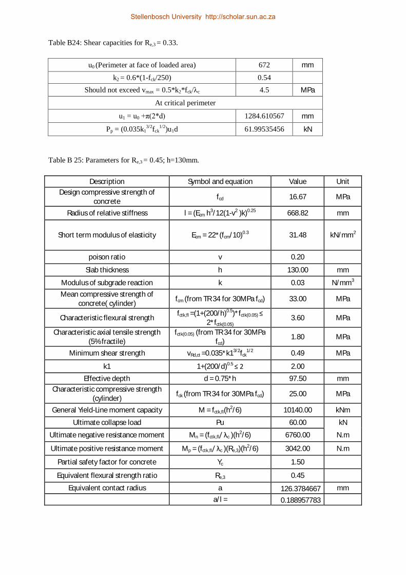
Table B24: Shear capacities for Re,3 = 0.33.
u0 (Perimeter at face of loaded area) 672 mm
k2 = 0.6*(1-fck/250) 0.54
Should not exceed vmax = 0.5*k2*fck/λc 4.5 MPa
At critical perimeter
u1 = u0 +π(2*d) 1284.610567 mm
Pp = (0.035k13/2fck
1/2)u1d 61.99535456 kN
Table B 25: Parameters for Re,3 = 0.45; h=130mm.
Description Symbol and equation Value Unit Design compressive strength of
concrete fcd 16.67 MPa
Radius of relative stiffness l = (Ecm h3/12(1-v2 )k)0.25 668.82 mm
Short term modulus of elasticity Ecm = 22*(fcm/10)0.3 31.48 kN/mm2
poison ratio v 0.20
Slab thickness h 130.00 mm
Modulus of subgrade reaction k 0.03 N/mm3
Mean compressive strength of concrete( cylinder)
fcm (from TR 34 for 30MPa fcd) 33.00 MPa
Characteristic flexural strength fctk,fl =(1+(200/h)0.5)*fctk(0.05) ≤
2*fctk(0.05) 3.60 MPa
Characteristic axial tensile strength (5% fractile)
fctk(0.05) (from TR 34 for 30MPa fcd)
1.80 MPa
Minimum shear strength vRd,ct =0.035*k13/2fck1/2 0.49 MPa
k1 1+(200/d)0.5 ≤ 2 2.00
Effective depth d = 0.75*h 97.50 mm Characteristic compressive strength
(cylinder) fck (from TR 34 for 30MPa fcd) 25.00 MPa
General Yield-Line moment capacity M = fctk,fl(h2/6) 10140.00 kNm
Ultimate collapse load Pu 60.00 kN
Ultimate negative resistance moment Mn = (fctk,fl/ λc )(h2/6) 6760.00 N.m
Ultimate positive resistance moment Mp = (fctk,fl/ λc )(Re,3)(h2/6) 3042.00 N.m
Partial safety factor for concrete Yc 1.50
Equivalent flexural strength ratio Re,3 0.45
Equivalent contact radius a 126.3784667 mm
a/l = 0.188957783
Stellenbosch University http://scholar.sun.ac.za

Table B 26: Ultimate load capacities for Re,3 = 0.45.
a/l a/l a/l 0 >0.2 126.38 0.00 >0.2 126.38 0.00 >0.2 126.38
Internal Load (kN) Edge Load (kN) Corner Load (kN)
61.6 131.5 127.6 28.9 66.2 64.1 13.5 33.3 32.2
Table B27: Shear capacities for Re,3 = 0.45.
u0 (Perimeter at face of loaded area) 672 mm
k2 = 0.6*(1-fck/250) 0.54
Should not exceed vmax = 0.5*k2*fck/λc 4.5 MPa
At critical perimeter
u1 = u0 +π(2*d) 1284.610567 mm
Pp = (0.035k13/2fck
1/2)u1d 61.99535456 kN
Stellenbosch University http://scholar.sun.ac.za

60kN Post Load
Table B 28: Parameters for Re,3 = 0; h=160mm.
Description Symbol and equation Value Unit Design compressive strength of
concrete fcd 16.67 MPa
Radius of relative stiffness l = (Ecm h3/12(1-v2 )k)0.25 781.52 mm
Short term modulus of elasticity Ecm = 22*(fcm/10)0.3 31.48 kN/m
m2
poison ratio v 0.20
Slab thickness h 160.00 mm
Modulus of subgrade reaction k 0.03 N/mm
3 Mean compressive strength of
concrete( cylinder) fcm (from TR 34 for 30MPa fcd) 33.00 MPa
Characteristic flexural strength fctk,fl =(1+(200/h)0.5)*fctk(0.05) ≤
2*fctk(0.05) 3.60 MPa
Characteristic axial tensile strength (5% fractile)
fctk(0.05) (from TR 34 for 30MPa fcd) 1.80 MPa
Minimum shear strength vRd,ct =0.035*k13/2fck1/2 0.49 MPa
k1 1+(200/d)0.5 ≤ 2 2.00
Effective depth d = 0.75*h 120.00 mm Characteristic compressive
strength (cylinder) fck (from TR 34 for 30MPa fcd) 25.00 MPa
General Yield-Line moment capacity
M = fctk,fl(h2/6) 15360.00 kNm
Ultimate collapse load Pu 72.00 kN Ultimate negative resistance
moment Mn = (fctk,fl/ λc )(h
2/6) 10240.00 N.m
Ultimate positive resistance moment
Mp = (fctk,fl/ λc )(Re,3)(h2/6) 0.00 N.m
Partial safety factor for concrete Yc 1.50
Equivalent flexural strength ratio Re,3 0.00
Equivalent contact radius a 126.3784667 mm
a/l = 0.1617083
Table B 29: Ultimate load capacities for Re,3 = 0.
a/l a/l a/l 0 >0.2 126.38 0.00 >0.2 126.38 0.00 >0.2 126.38
Internal Load (kN) Edge Load (kN) Corner Load (kN)
64.3 136.0 122.3 36.6 82.0 73.3 20.5 48.9 43.4
Stellenbosch University http://scholar.sun.ac.za

Table B30: Shear capacities for Re,3 = 0.
u0 (Perimeter at face of loaded area) 672 mm
k2 = 0.6*(1-fck/250) 0.54
Should not exceed vmax = 0.5*k2*fck/λc 4.5 MPa
At critical perimeter
u1 = u0 +π(2*d) 1425.982237 mm
Pp = (0.035k13/2fck
1/2)u1d 84.6990236 kN
Table B 31: Parameters for Re,3 = 0.2; h=150mm.
Description Symbol and equation Value Unit Design compressive strength of concrete
fcd 16.67 MPa
Radius of relative stiffness l = (Ecm h3/12(1-v2 )k)0.25 744.59 mm
Short term modulus of elasticity
Ecm = 22*(fcm/10)0.3 31.48 kN/mm2
poison ratio v 0.20
Slab thickness h 150.00 mm Modulus of subgrade
reaction k 0.03 N/mm3
Mean compressive strength of concrete( cylinder)
fcm (from TR 34 for 30MPa fcd) 33.00 MPa
Characteristic flexural strength
fctk,fl =(1+(200/h)0.5)*fctk(0.05) ≤ 2*fctk(0.05)
3.60 MPa
Characteristic axial tensile strength (5% fractile)
fctk(0.05) (from TR 34 for 30MPa fcd) 1.80 MPa
Minimum shear strength vRd,ct =0.035*k13/2fck1/2 0.49 MPa
k1 1+(200/d)0.5 ≤ 2 2.00
Effective depth d = 0.75*h 112.50 mm Characteristic compressive
strength (cylinder) fck (from TR 34 for 30MPa fcd) 25.00 MPa
General Yield-Line moment capacity
M = fctk,fl(h2/6) 13500.00 kNm
Ultimate collapse load Pu 72.00 kN Ultimate negative
resistance moment Mn = (fctk,fl/ λc )(h
2/6) 9000.00 N.m
Ultimate positive resistance moment
Mp = (fctk,fl/ λc )(Re,3)(h2/6) 1800.00 N.m
Partial safety factor for concrete
Yc 1.50
Equivalent flexural strength ratio
Re,3 0.20
Equivalent contact radius a 126.3784667 mm a/l = 0.169728141
Stellenbosch University http://scholar.sun.ac.za

Table B 32: Ultimate load capacities for Re,3 = 0.2.
a/l a/l a/l 0 >0.2 126.38 0.00 >0.2 126.38 0.00 >0.2 126.38
Internal Load (kN) Edge Load (kN) Corner Load (kN)
67.9 143.9 132.4 35.0 78.9 72.2 18.0 43.4 39.5
Table B33: Shear capacities for Re,3 = 0.2.
u0 (Perimeter at face of loaded area) 672 mm
k2 = 0.6*(1-fck/250) 0.54
Should not exceed vmax = 0.5*k2*fck/λc 4.5 MPa
At critical perimeter
u1 = u0 +π(2*d) 1378.858347 mm
Pp = (0.035k13/2fck
1/2)u1d 76.78125689 kN
Stellenbosch University http://scholar.sun.ac.za

Table B 34: Parameters for Re,3 = 0.33; h=145mm.
Description Symbol and equation Value Unit Design compressive strength of
concrete fcd 16.67 MPa
Radius of relative stiffness l = (Ecm h3/12(1-v2 )k)0.25 725.90 mm
Short term modulus of elasticity Ecm = 22*(fcm/10)0.3 31.48 kN/mm2
poison ratio v 0.20
Slab thickness h 145.00 mm
Modulus of subgrade reaction k 0.03 N/mm3
Mean compressive strength of concrete( cylinder)
fcm (from TR 34 for 30MPa fcd) 33.00 MPa
Characteristic flexural strength fctk,fl =(1+(200/h)0.5)*fctk(0.05) ≤
2*fctk(0.05) 3.60 MPa
Characteristic axial tensile strength (5% fractile)
fctk(0.05) (from TR 34 for 30MPa fcd) 1.80 MPa
Minimum shear strength vRd,ct =0.035*k13/2fck1/2 0.49 MPa
k1 1+(200/d)0.5 ≤ 2 2.00
Effective depth d = 0.75*h 108.75 mm Characteristic compressive
strength (cylinder) fck (from TR 34 for 30MPa fcd) 25.00 MPa
General Yield-Line moment capacity
M = fctk,fl(h2/6) 12615.00 kNm
Ultimate collapse load Pu 72.00 kN Ultimate negative resistance
moment Mn = (fctk,fl/ λc )(h
2/6) 8410.00 N.m
Ultimate positive resistance moment
Mp = (fctk,fl/ λc )(Re,3)(h2/6) 2775.30 N.m
Partial safety factor for concrete Yc 1.50
Equivalent flexural strength ratio Re,3 0.33
Equivalent contact radius a 126.3784667 mm
a/l = 0.174099009
Table B 35: Ultimate load capacities for Re,3 = 0.33.
a/l a/l a/l 0 >0.2 126.38 0.00 >0.2 126.38 0.00 >0.2 126.38
Internal Load (kN) Edge Load (kN) Corner Load (kN)
70.3 149.2 139.0 34.4 77.8 72.2 16.8 40.7 37.6
Stellenbosch University http://scholar.sun.ac.za

Table B36: Shear capacities for Re,3 = 0.33.
u0 (Perimeter at face of loaded area) 672 mm
k2 = 0.6*(1-fck/250) 0.54
Should not exceed vmax = 0.5*k2*fck/λc 4.5 MPa
At critical perimeter
u1 = u0 +π(2*d) 1355.296402 mm
Pp = (0.035k13/2fck
1/2)u1d 72.95357742 kN
Table B 37: Parameters for Re,3 = 0.45; h=145mm.
Description Symbol and equation Value Unit Design compressive strength of
concrete fcd 16.67 MPa
Radius of relative stiffness l = (Ecm h3/12(1-v2 )k)0.25 725.90 mm
Short term modulus of elasticity Ecm = 22*(fcm/10)0.3 31.48 kN/mm2
poison ratio v 0.20
Slab thickness h 145.00 mm
Modulus of subgrade reaction k 0.03 N/mm3
Mean compressive strength of concrete( cylinder)
fcm (from TR 34 for 30MPa fcd) 33.00 MPa
Characteristic flexural strength fctk,fl =(1+(200/h)0.5)*fctk(0.05) ≤
2*fctk(0.05) 3.60 MPa
Characteristic axial tensile strength (5% fractile)
fctk(0.05) (from TR 34 for 30MPa fcd)
1.80 MPa
Minimum shear strength vRd,ct =0.035*k13/2fck1/2 0.49 MPa
k1 1+(200/d)0.5 ≤ 2 2.00
Effective depth d = 0.75*h 108.75 mm Characteristic compressive
strength (cylinder) fck (from TR 34 for 30MPa fcd) 25.00 MPa
General Yield-Line moment capacity
M = fctk,fl(h2/6) 12615.00 kNm
Ultimate collapse load Pu 72.00 kN Ultimate negative resistance
moment Mn = (fctk,fl/ λc )(h
2/6) 8410.00 N.m
Ultimate positive resistance moment
Mp = (fctk,fl/ λc )(Re,3)(h2/6) 3784.50 N.m
Partial safety factor for concrete Yc 1.50
Equivalent flexural strength ratio Re,3 0.45
Equivalent contact radius a 126.3784667 mm
a/l = 0.174099009
Stellenbosch University http://scholar.sun.ac.za

Table B 38: Ultimate load capacities for Re,3 = 0.45.
a/l a/l a/l 0 >0.2 126.38 0.00 >0.2 126.38 0.00 >0.2 126.38
Internal Load (kN) Edge Load (kN) Corner Load (kN)
76.6 162.7 151.5 36.0 81.4 75.5 16.8 40.7 37.6
Table B39: Shear capacities for Re,3 = 0.45.
u0 (Perimeter at face of loaded area) 672 mm
k2 = 0.6*(1-fck/250) 0.54
Should not exceed vmax = 0.5*k2*fck/λc 4.5 MPa
At critical perimeter
u1 = u0 +π(2*d) 1355.296402 mm
Pp = (0.035k13/2fck
1/2)u1d 72.95357742 kN
Stellenbosch University http://scholar.sun.ac.za

Addendum C
Stellenbosch University http://scholar.sun.ac.za

Checks to confirm the capacity of the slabs designed for Chapter 7 by using the
Westegaard theory.
Design for the large loading plate:
Bearing capacity
Allowable stress :
Interior: 4.2 x ff = 4.2 x 3.8 = 15.96 MPa
Edge or corner = 2.1 x ff = 2.1 x 3.8 = 7.98 MPa
Computed stress:
Ultimate load/contact area = 42.5 x 10³/67.5 x 10-3 = 0.63 MPa
This means that the bearing resistance of the slab is sufficient since 0.63 < 7.98- and 15.96MPa.
Shear stresses
Allowable shear stress:
Marais & Perrie (1993) recommends that a shear capacity of 0.27 times the flexural strength at 28 days
should be used.
0.27 x ff = 0.27 x 3.8 = 1.026MPa
This maximum stress should now be checked for interior-, edge- and corner loading conditions.
Interior:
= load
slab depth[(load periphery) + 4(slab depth)]
=42500
120 ∗ (1200 + 4 ∗ 120)
= 0.2108 푀푃푎
Edge:
=post load
slab depth[0.75 ∗ (load periphery) + 2 ∗ (slab depth)]
Stellenbosch University http://scholar.sun.ac.za

=42500
120 ∗ (0.75 ∗ (1200) + 2 ∗ 120)
= 0.3107 푀푃푎
Corner:
=Post load
slab depth ∗ [0.5 ∗ (load periphery) + (slab depth)]
=42500
120 ∗ (0.5 ∗ 1200 + 120)
= 0.4919 푀푃푎
The shear capacity of the slab is sufficient for a load of 42.5kN.
Design for the small loading plate:
Bearing capacity
Computed stress:
Ultimate load/contact area = 32.5 x 10³/5 x 10-3 = 6.5MPa
This means that the bearing resistance of the slab is sufficient since 6.5 < 7.98 and 15.96MPa.
Shear stresses:
Allowable shear stress:
0.27 x ff = 0.27 x 3.8 = 1.026MPa
This maximum stress should now be checked for interior-, edge- and corner loading conditions.
Interior:
= load
slab depth[(load periphery) + 4(slab depth)]
=32500
120 ∗ (300 + 4 ∗ 120)
= 0.3472 푀푃푎
Edge:
Stellenbosch University http://scholar.sun.ac.za

=post load
slab depth[0.75 ∗ (load periphery) + 2 ∗ (slab depth)]
=32500
120 ∗ (0.75 ∗ (300) + 2 ∗ 120)
= 0.5824 푀푃푎
Corner:
=Post load
slab depth ∗ [0.5 ∗ (load periphery) + (slab depth)]
=32500
120 ∗ (0.5 ∗ 300 + 120)
= 1.003 푀푃푎
The shear capacity of the slab is sufficient for the load of 32.5kN.
Stellenbosch University http://scholar.sun.ac.za