The Stratospheric Response to 11-Year Solar Variability ...

Global Change and the Solar-Terrestrial Environment Aspen, Colorado June 13, 2010

The Stratospheric Response to 11-Year Solar Variability: Direct UV Forcing and the Possible Role of Ocean-Troposphere Feedbacks*

Lon Hood Lunar & Planetary Laboratory University of Arizona USA

*With assistance from Boris Soukharev and John McCormack

Solar Production of Ozone and Ozone Heating of the Stratosphere:

Alti

tude

, km

David Fahey, WMO/UNEP Ozone Assessment Report (2002)

Nolan Adkins, Lyndon State College

λ < 242 nm:

λ > 200 nm:

Variability of Solar UV Flux Occurring on Both the 27-Day and 11-Year Time Scales

205 nm Solar Flux

(Nimbus 7 SBUV)

Direct Solar UV Forcing of Stratospheric Ozone (27-day Time Scale):

Hood, JGR, 1986

Time series are filtered to minimize variations at periods > 35 days.

The maximum ozone response to short-term solar UV variations occurs near the 2 hPa level (42 km altitude) and amounts to about 0.5 per cent for a 1 per cent change in the 205 nm flux. These responses were measured at low latitudes (25oS – 25oN).

Hood and Cantrell, Annal. Geophysicae, 1988

McCormack and Hood, JGR, 1996

65oS to 65oN

65oS to 65oN

Direct Solar UV Forcing of Stratospheric Ozone and Temperature (11-Year Time Scale):

Question: Why is it important to determine and understand the stratospheric response (e.g., ozone) to 11-year solar forcing?

Answer: Because, as shown originally by Joanna Haigh (1996; 1999), the solar-induced change in stratospheric ozone produces perturbations of tropospheric circulation and climate. Moreover, the amplitude of these perturbations is sensitive to the actual change in ozone in the stratosphere and its distribution.

Question: Why is it important to determine and understand the stratospheric response (e.g., ozone) to 11-year solar forcing?

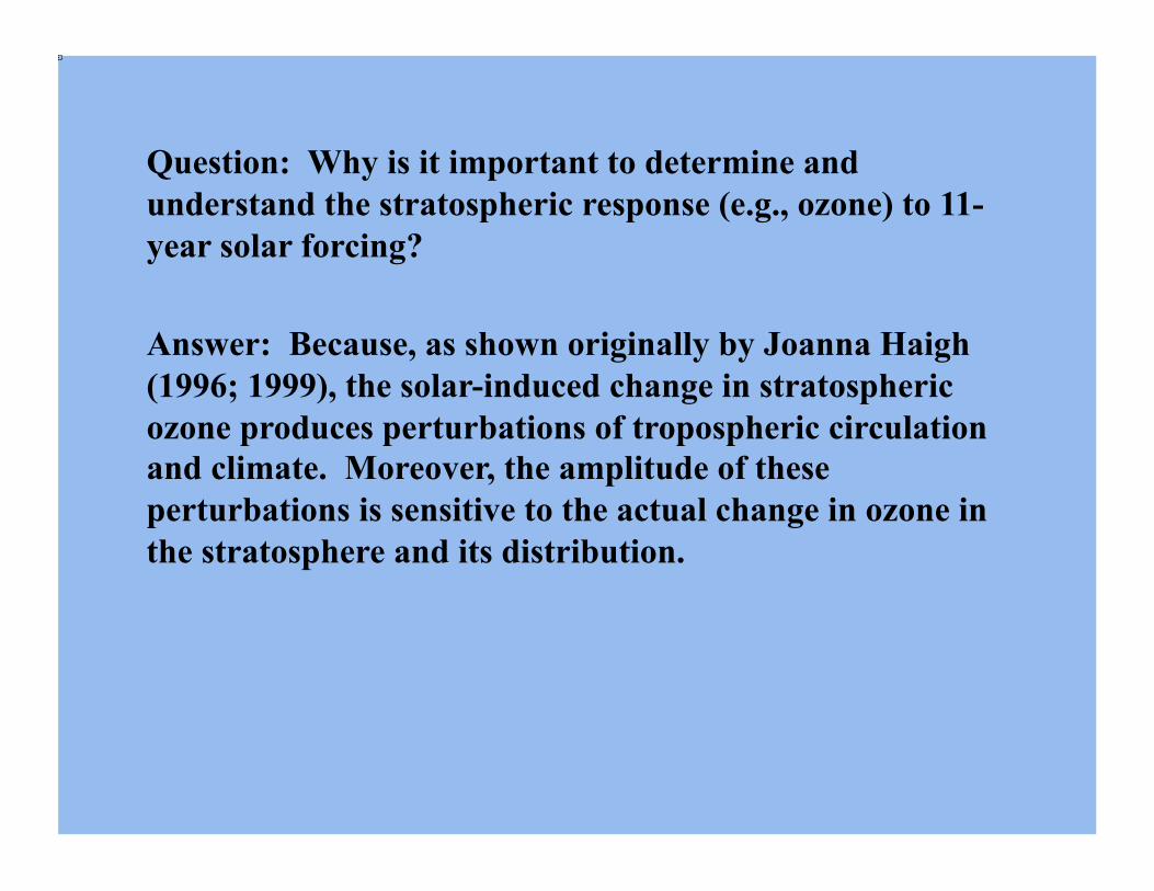
Three sources of decadal-scale variability of total ozone in the Version 8 TOMS/SBUV data record calibrated by Frith et al. (2004): A non-linear long-term trend, volcanic aerosol forcing, and the 11-year solar cycle.

C

P

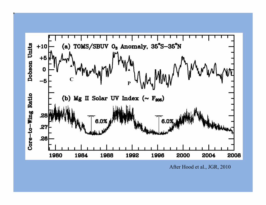
After Hood et al., JGR, 2010

C P

Model Simulation of the Solar Cycle Variation of Stratospheric Ozone Considering Only the Direct Photochemical Effects of Solar Cycle UV Variations:

Model Data Courtesy of Drew Shindell, 2004

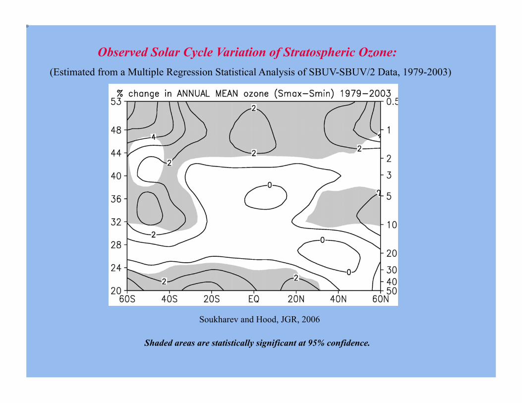
Observed Solar Cycle Variation of Stratospheric Ozone:

Soukharev and Hood, JGR, 2006

(Estimated from a Multiple Regression Statistical Analysis of SBUV-SBUV/2 Data, 1979-2003)

Shaded areas are statistically significant at 95% confidence.

Contrast between observed ozone solar cycle response and that simulated by a photochemical transport model:

Model Data courtesy of Drew Shindell, 2004

Observations: Models:

From Soukharev & Hood, 2006

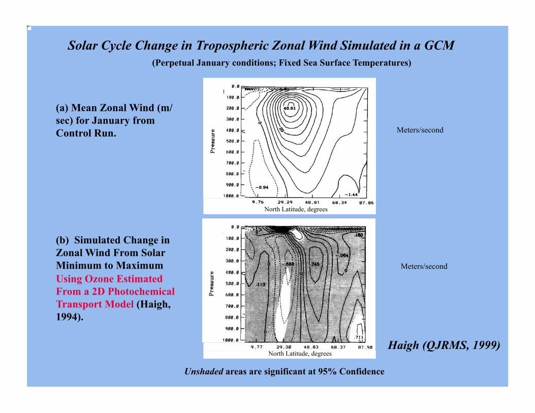
(a) Mean Zonal Wind (m/sec) for January from Control Run.

Solar Cycle Change in Tropospheric Zonal Wind Simulated in a GCM (Perpetual January conditions; Fixed Sea Surface Temperatures)

Unshaded areas are significant at 95% Confidence

Meters/second

Meters/second

Haigh (QJRMS, 1999)

North Latitude, degrees

(b) Simulated Change in Zonal Wind From Solar Minimum to Maximum Using Ozone Estimated From a 2D Photochemical Transport Model (Haigh, 1994).


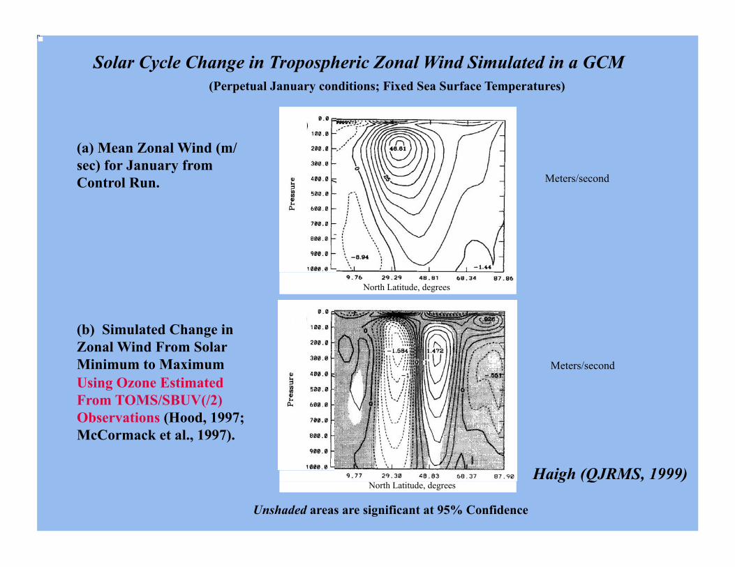
(a) Mean Zonal Wind (m/sec) for January from Control Run.

Solar Cycle Change in Tropospheric Zonal Wind Simulated in a GCM (Perpetual January conditions; Fixed Sea Surface Temperatures)


Meters/second

Meters/second

Haigh (QJRMS, 1999)


(b) Simulated Change in Zonal Wind From Solar Minimum to Maximum Using Ozone Estimated From TOMS/SBUV(/2) Observations (Hood, 1997; McCormack et al., 1997).


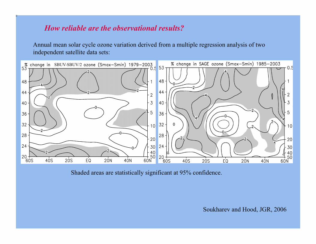
Annual mean solar cycle ozone variation derived from a multiple regression analysis of two independent satellite data sets:

Shaded areas are statistically significant at 95% confidence.

SBUV-SBUV/2

Soukharev and Hood, JGR, 2006

How reliable are the observational results?

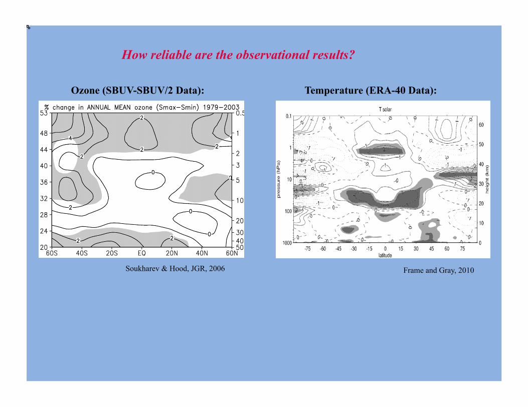
Frame and Gray, 2010

Ozone (SBUV-SBUV/2 Data): Temperature (ERA-40 Data):

Soukharev & Hood, JGR, 2006


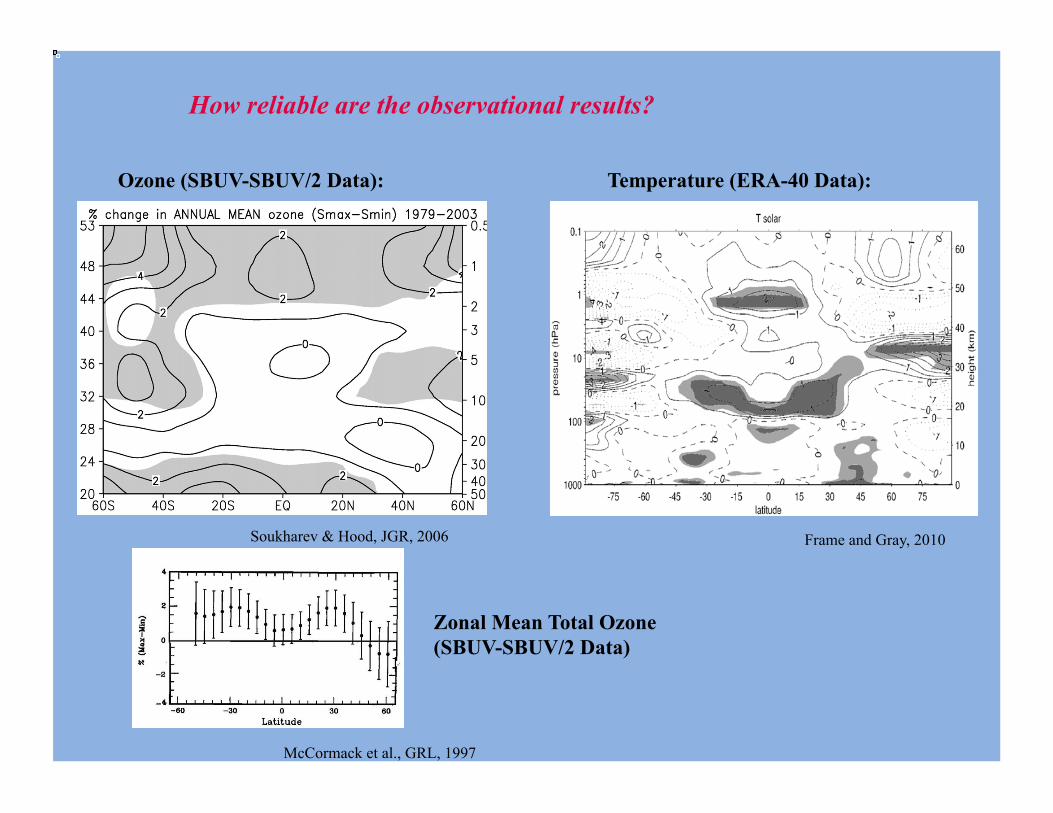
Frame and Gray, 2010

Ozone (SBUV-SBUV/2 Data): Temperature (ERA-40 Data):

Soukharev & Hood, JGR, 2006

McCormack et al., GRL, 1997

Zonal Mean Total Ozone (SBUV-SBUV/2 Data)


Question: What is causing this unexpected vertical structure in the stratospheric response to 11-year solar forcing? In particular, why is there a strong response in the tropical lower stratosphere?

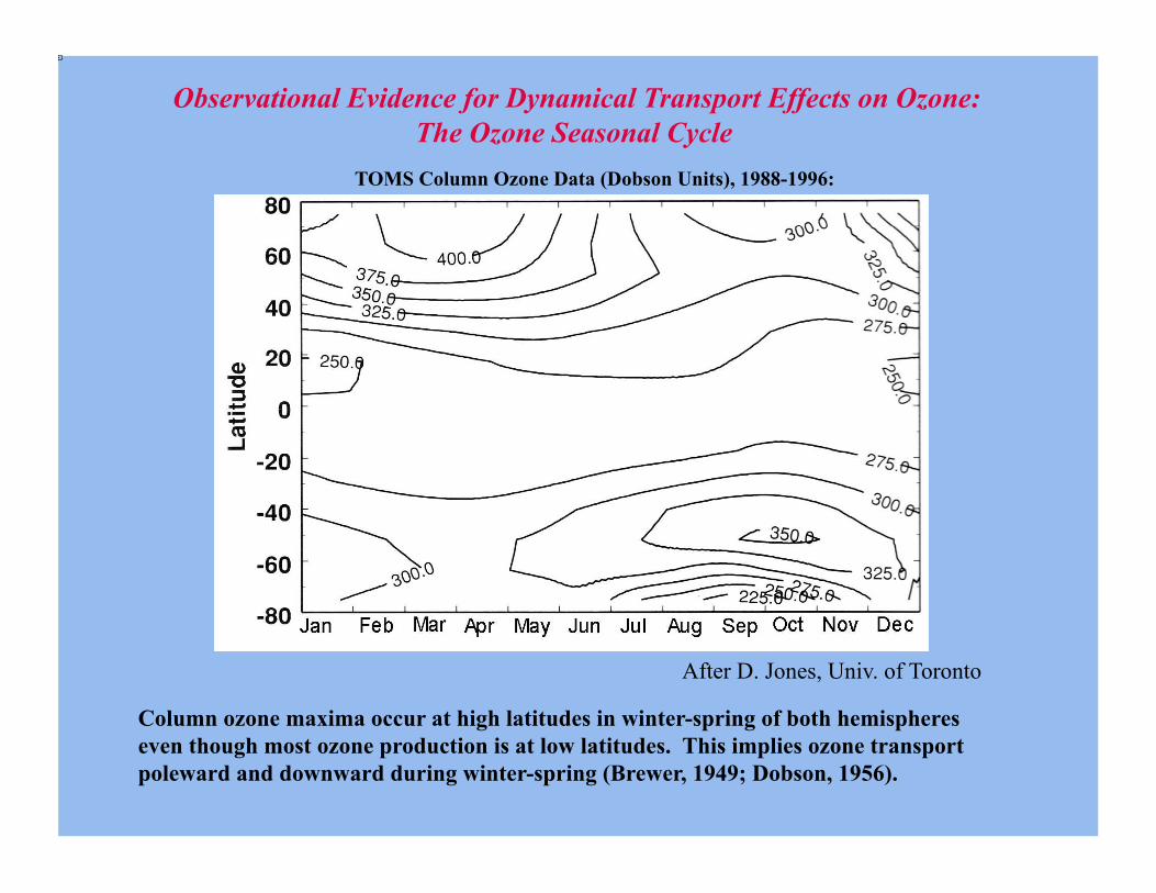
Observational Evidence for Dynamical Transport Effects on Ozone: The Ozone Seasonal Cycle

TOMS Column Ozone Data (Dobson Units), 1988-1996:

After D. Jones, Univ. of Toronto

Column ozone maxima occur at high latitudes in winter-spring of both hemispheres even though most ozone production is at low latitudes. This implies ozone transport poleward and downward during winter-spring (Brewer, 1949; Dobson, 1956).

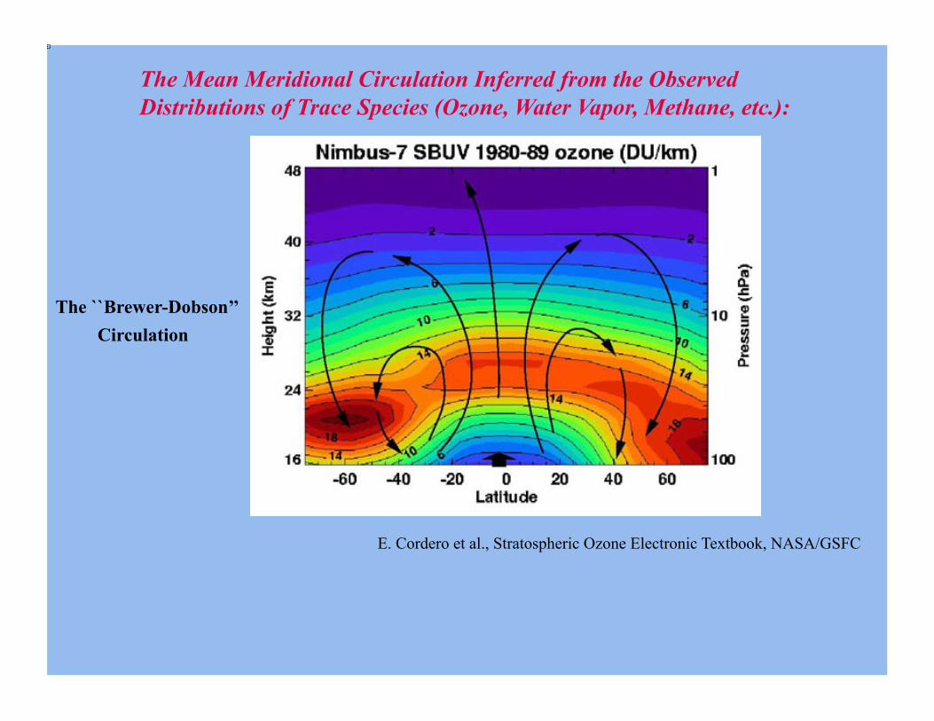
The Mean Meridional Circulation Inferred from the Observed Distributions of Trace Species (Ozone, Water Vapor, Methane, etc.):

E. Cordero et al., Stratospheric Ozone Electronic Textbook, NASA/GSFC

The ``Brewer-Dobson’’ Circulation

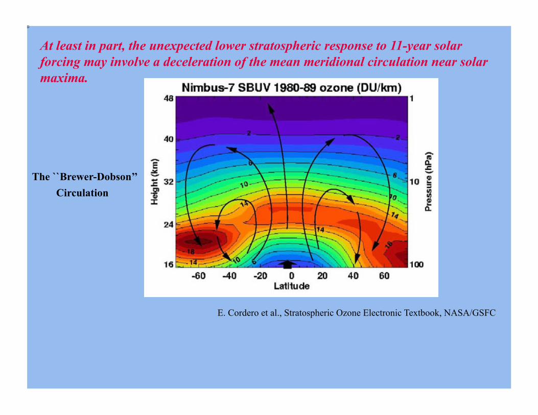
At least in part, the unexpected lower stratospheric response to 11-year solar forcing may involve a deceleration of the mean meridional circulation near solar maxima.

E. Cordero et al., Stratospheric Ozone Electronic Textbook, NASA/GSFC

The ``Brewer-Dobson’’ Circulation

(1) Top-Down: Direct UV forcing in the upper stratosphere perturbs stratospheric circulation in such a way as to modulate the Brewer-Dobson circulation.

Two Candidate Mechanisms:

(2) Bottom-Up: Feedbacks from an ocean-troposphere response to solar variability (driven by both total irradiance changes and indirect effects of the stratospheric response) may also modulate the Brewer-Dobson circulation.

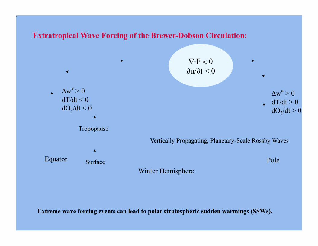
∇⋅F < 0 ∂u/∂t < 0

Vertically Propagating, Planetary-Scale Rossby Waves

Pole Equator

Tropopause

Δw* > 0 dT/dt < 0 dO3/dt < 0

Δw* > 0 dT/dt > 0 dO3/dt > 0

Winter Hemisphere

Extratropical Wave Forcing of the Brewer-Dobson Circulation:

Surface

Extreme wave forcing events can lead to polar stratospheric sudden warmings (SSWs).

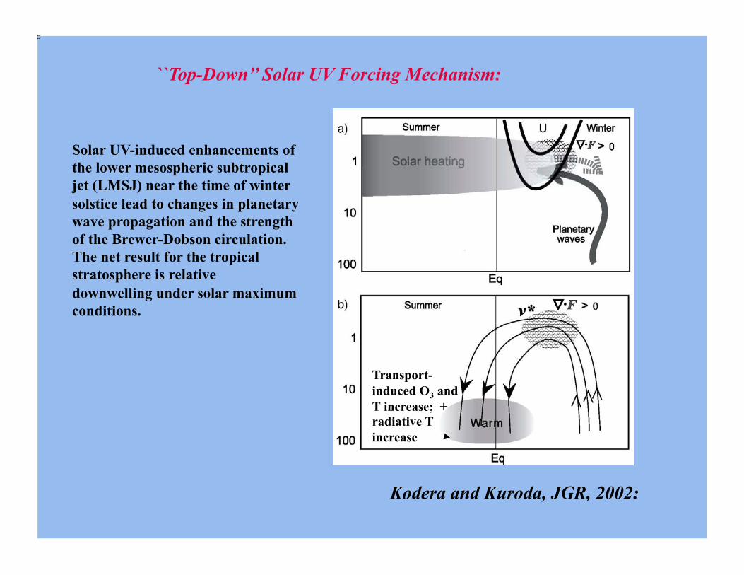
Solar UV-induced enhancements of the lower mesospheric subtropical jet (LMSJ) near the time of winter solstice lead to changes in planetary wave propagation and the strength of the Brewer-Dobson circulation. The net result for the tropical stratosphere is relative downwelling under solar maximum conditions.

Kodera and Kuroda, JGR, 2002:

Transport-induced O3 and T increase; + radiative T increase

``Top-Down’’ Solar UV Forcing Mechanism:

A number of observational and model studies have supported this mechanism: Gray et al., 2001a,b; 2003; 2004; 2007; Matthes et al., 2004; 2006.

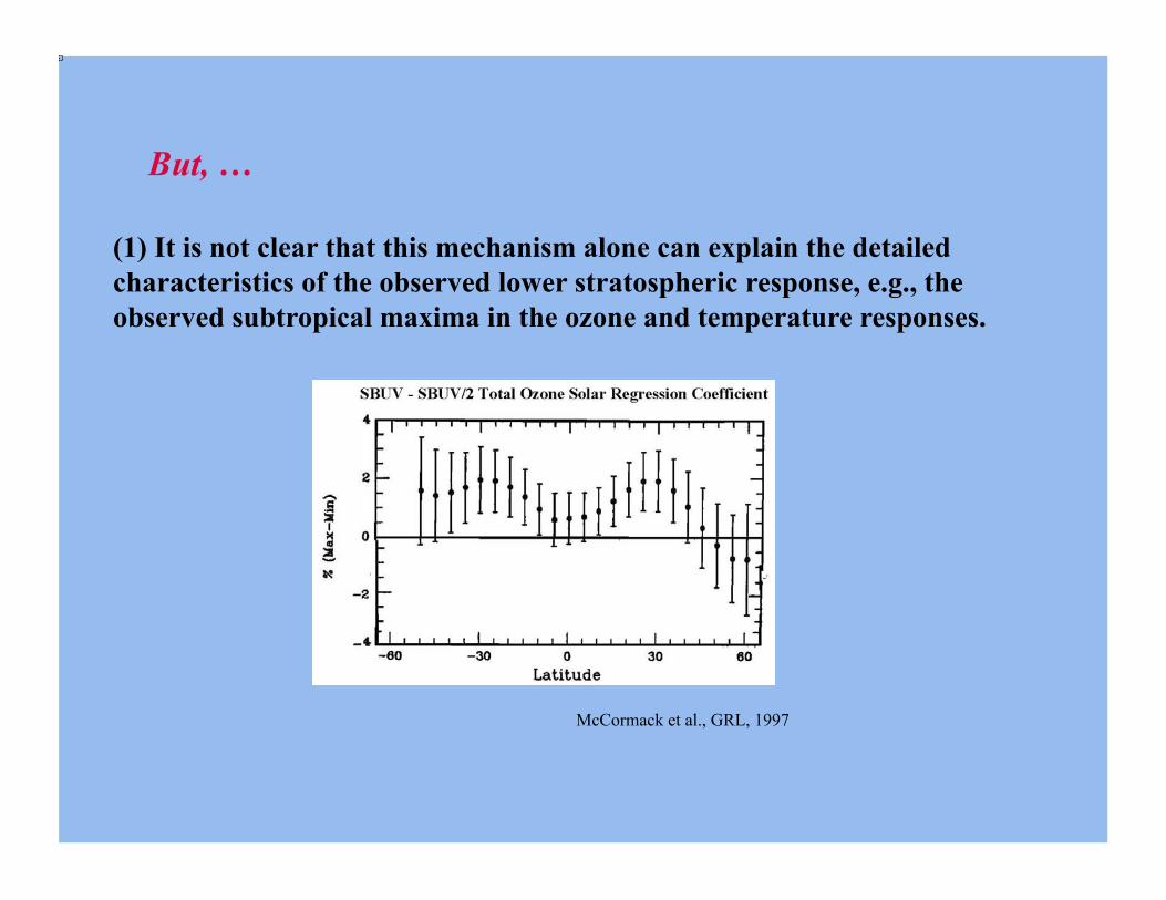
But, …

(1) It is not clear that this mechanism alone can explain the detailed characteristics of the observed lower stratospheric response, e.g., the observed subtropical maxima in the ozone and temperature responses.

McCormack et al., GRL, 1997

But, …

(1) It is not clear that this mechanism alone can explain the detailed characteristics of the observed lower stratospheric response, e.g., the observed subtropical maxima in the ozone and temperature responses.

(2) Most or all GCM simulations assuming only top-down forcing are not able to simulate the observed vertical structure of the tropical ozone response.

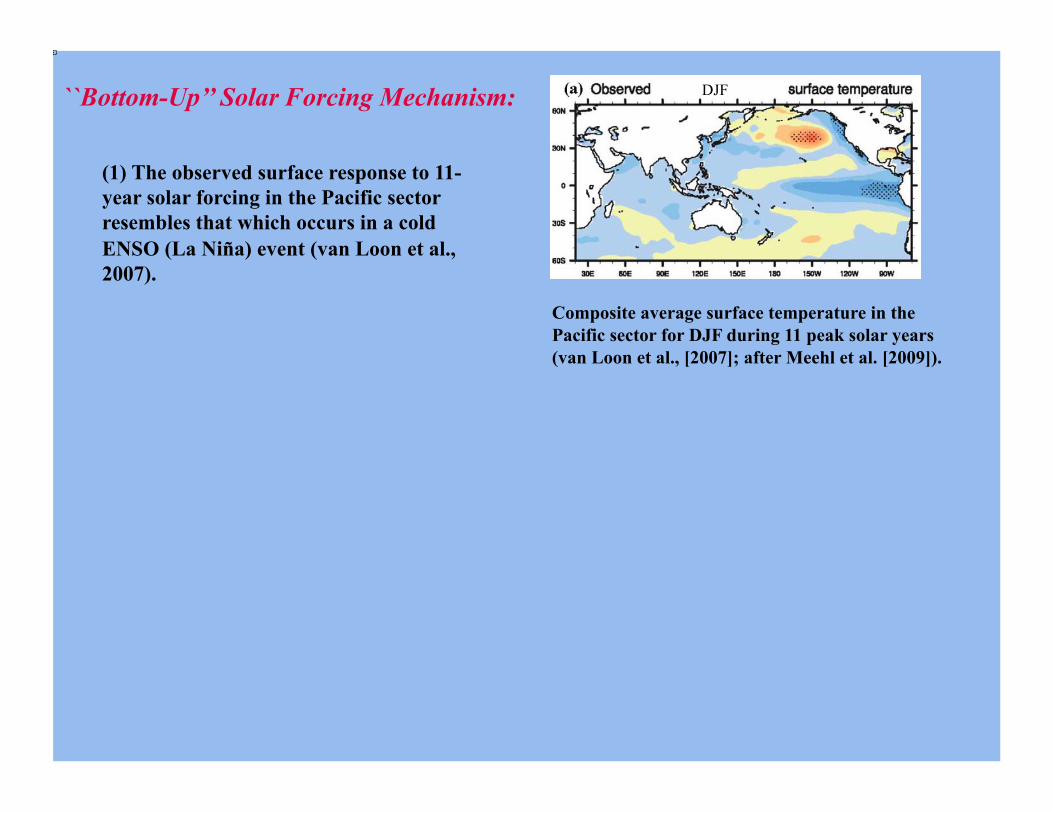
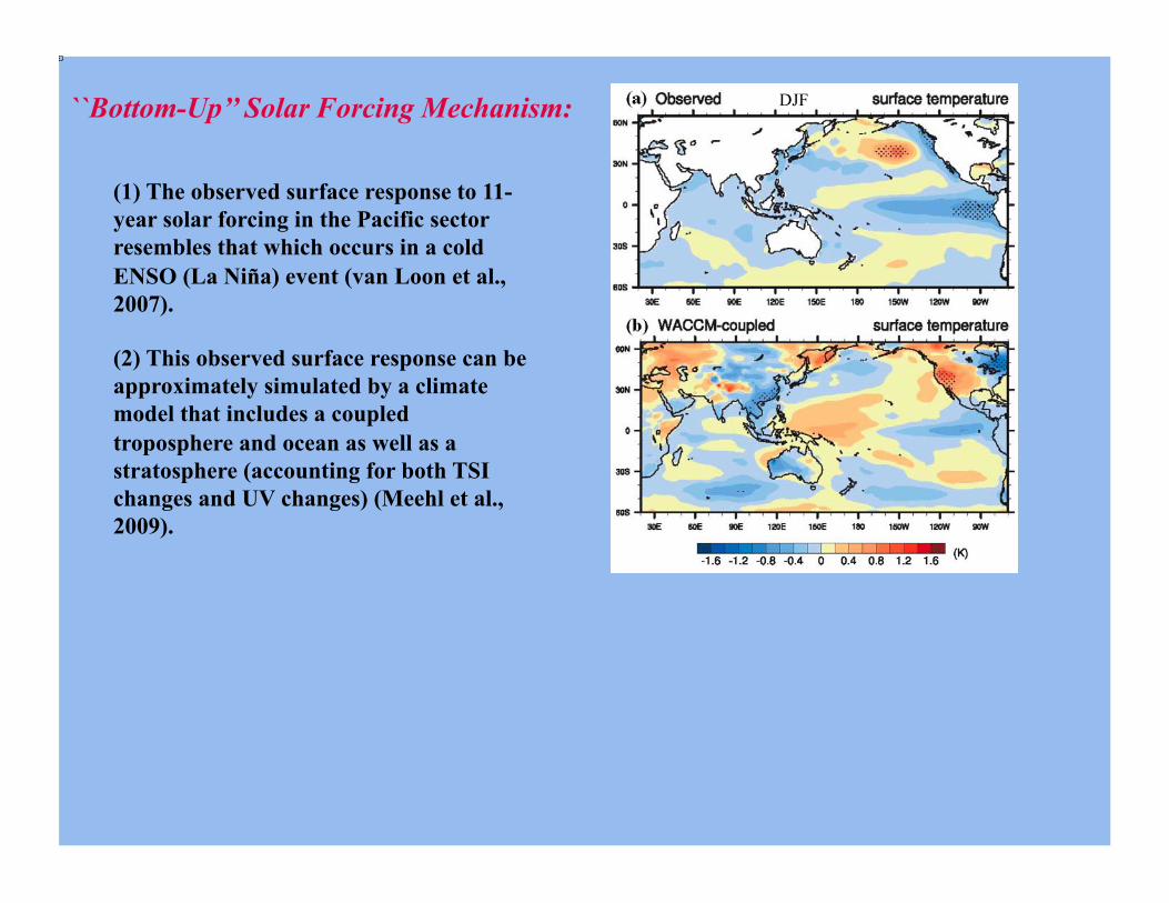
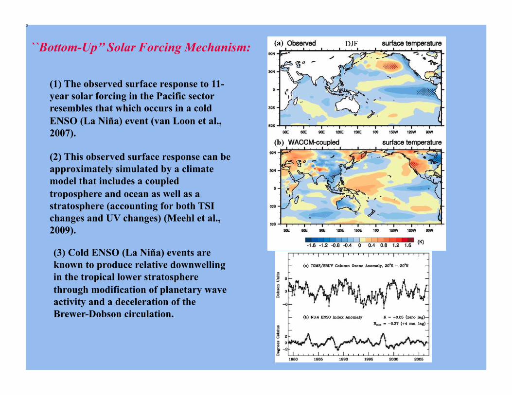
(1) The observed surface response to 11-year solar forcing in the Pacific sector resembles that which occurs in a cold ENSO (La Niña) event (van Loon et al., 2007).

``Bottom-Up’’ Solar Forcing Mechanism:

Composite average surface temperature in the Pacific sector for DJF during 11 peak solar years (van Loon et al., [2007]; after Meehl et al. [2009]).

DJF



(2) This observed surface response can be approximately simulated by a climate model that includes a coupled troposphere and ocean as well as a stratosphere (accounting for both TSI changes and UV changes) (Meehl et al., 2009).

DJF



(2) This observed surface response can be approximately simulated by a climate model that includes a coupled troposphere and ocean as well as a stratosphere (accounting for both TSI changes and UV changes) (Meehl et al., 2009).

(3) Cold ENSO (La Niña) events are known to produce relative downwelling in the tropical lower stratosphere through modification of planetary wave activity and a deceleration of the Brewer-Dobson circulation.

DJF

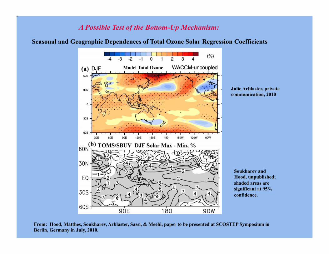
A Possible Test of the Bottom-Up Mechanism:

Soukharev and Hood, unpublished

Seasonal and Geographic Dependences of Total Ozone Solar Regression Coefficients

Shaded areas are significant at 95% confidence.


Soukharev and Hood, unpublished; shaded areas are significant at 95% confidence.


Julie Arblaster, private communication, 2010

From: Hood, Matthes, Soukharev, Arblaster, Sassi, & Meehl, paper to be presented at SCOSTEP Symposium in Berlin, Germany in July, 2010.

Model Total Ozone


Soukharev and Hood, unpublished; shaded areas are significant at 95% confidence.


Julie Arblaster, private communication, 2010

From: Hood, Matthes, Soukharev, Arblaster, Sassi, & Meehl, paper to be presented at SCOSTEP Symposium in Berlin, Germany in July, 2010.

Model Total Ozone (a)

Vertically Propagating, Planetary-Scale Rossby Waves

Pole Equator

Tropopause

Δw* < 0 dT/dt > 0 dO3/dt > 0

Winter Hemisphere

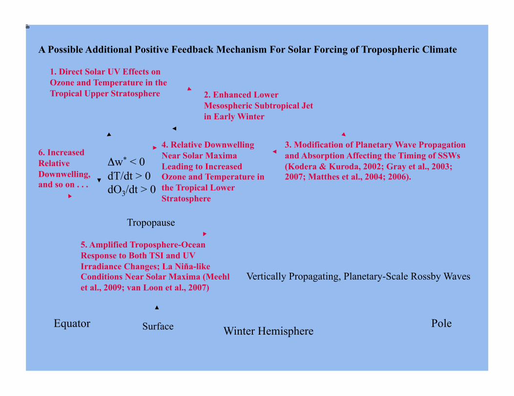
1. Direct Solar UV Effects on Ozone and Temperature in the Tropical Upper Stratosphere

Surface

2. Enhanced Lower Mesospheric Subtropical Jet in Early Winter

3. Modification of Planetary Wave Propagation and Absorption Affecting the Timing of SSWs (Kodera & Kuroda, 2002; Gray et al., 2003; 2007; Matthes et al., 2004; 2006).

4. Relative Downwelling Near Solar Maxima Leading to Increased Ozone and Temperature in the Tropical Lower Stratosphere

5. Amplified Troposphere-Ocean Response to Both TSI and UV Irradiance Changes; La Niña-like Conditions Near Solar Maxima (Meehl et al., 2009; van Loon et al., 2007)

6. Increased Relative Downwelling, and so on . . .

A Possible Additional Positive Feedback Mechanism For Solar Forcing of Tropospheric Climate

Contrast between observed ozone solar cycle response and that simulated by a photochemical transport model:

Model Data courtesy of Drew Shindell, 2004

Observations: Models:

From Soukharev & Hood, 2006

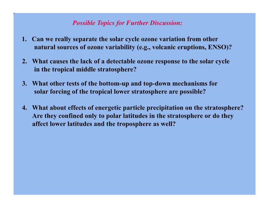
1. Can we really separate the solar cycle ozone variation from other

Possible Topics for Further Discussion:

2. What causes the lack of a detectable ozone response to the solar cycle in the tropical middle stratosphere?

natural sources of ozone variability (e.g., volcanic eruptions, ENSO)?

4. What about effects of energetic particle precipitation on the stratosphere? Are they confined only to polar latitudes in the stratosphere or do they affect lower latitudes and the troposphere as well?

3. What other tests of the bottom-up and top-down mechanisms for solar forcing of the tropical lower stratosphere are possible?

Solar UV-induced enhancements of the lower mesospheric subtropical jet (LMSJ) near the time of winter solstice lead to changes in planetary wave propagation and the strength of the Brewer-Dobson circulation. The net result for the tropical stratosphere is relative downwelling under solar maximum conditions.

Kodera and Kuroda, JGR, 2002:

Transport-induced O3 and T increase; + radiative T increase

``Top-Down’’ Solar UV Forcing Mechanism:

205 nm Solar Flux

(Nimbus 7 SAMS)

Direct Solar UV Forcing of Stratospheric Temperature (27-day Time Scale):

Hood, JGR, 1986

The maximum temperature response occurs near the stratopause (about 50 km altitude) and amounts to about 0.06 per cent (or 0.2 K) for a 1 per cent change in the 205 nm flux. These responses were measured at low latitudes (25oS – 25oN).

Hood and Cantrell, Annal. Geophysicae, 1988

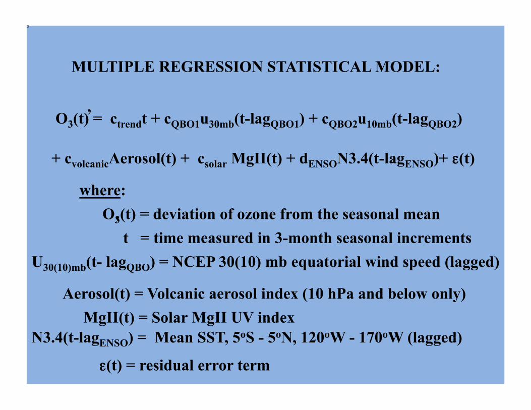
MULTIPLE REGRESSION STATISTICAL MODEL:

O3(t) = ctrendt + cQBO1u30mb(t-lagQBO1) + cQBO2u10mb(t-lagQBO2)

+ cvolcanicAerosol(t) + csolar MgII(t) + dENSON3.4(t-lagENSO)+ ε(t)

,

where:

t = time measured in 3-month seasonal increments O3(t) = deviation of ozone from the seasonal mean ,

U30(10)mb(t- lagQBO) = NCEP 30(10) mb equatorial wind speed (lagged)

Aerosol(t) = Volcanic aerosol index (10 hPa and below only) MgII(t) = Solar MgII UV index

ε(t) = residual error term

N3.4(t-lagENSO) = Mean SST, 5oS - 5oN, 120oW - 170oW (lagged)

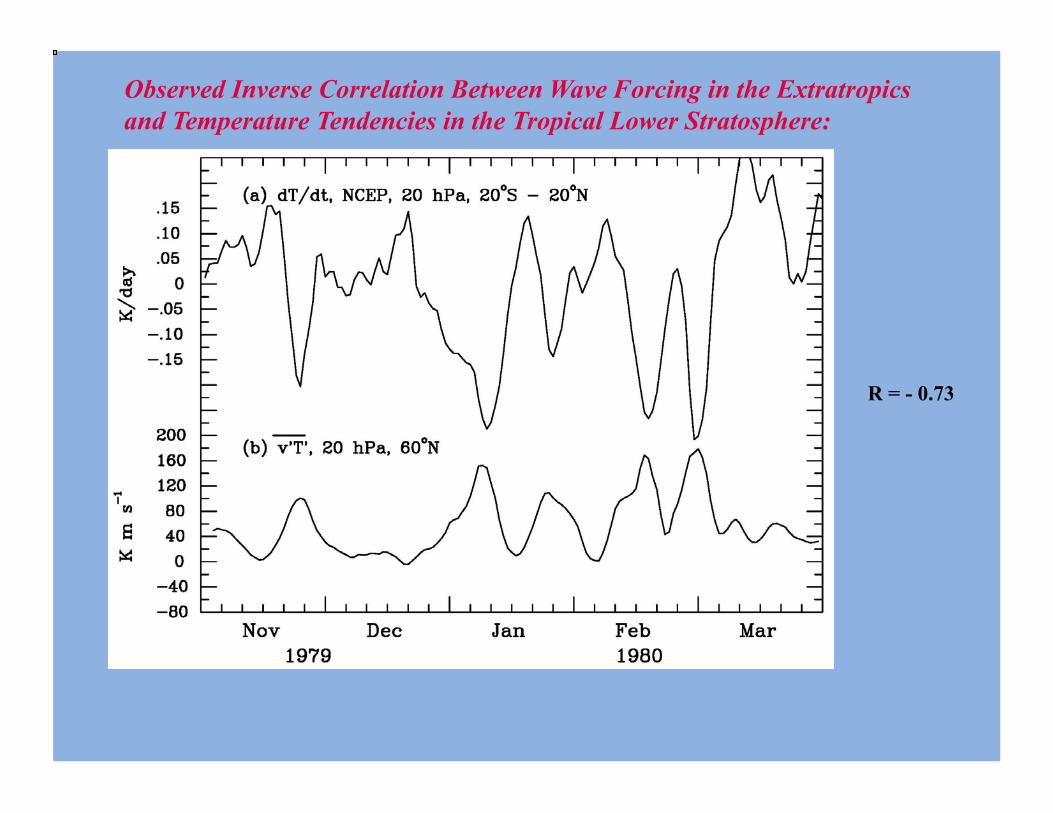
Observed Inverse Correlation Between Wave Forcing in the Extratropics and Temperature Tendencies in the Tropical Lower Stratosphere:

R = - 0.73

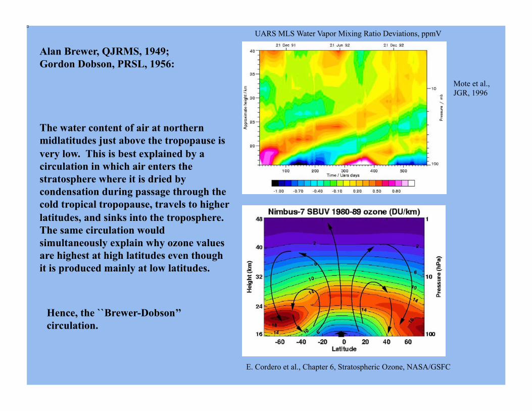
Alan Brewer, QJRMS, 1949; Gordon Dobson, PRSL, 1956:

The water content of air at northern midlatitudes just above the tropopause is very low. This is best explained by a circulation in which air enters the stratosphere where it is dried by condensation during passage through the cold tropical tropopause, travels to higher latitudes, and sinks into the troposphere. The same circulation would simultaneously explain why ozone values are highest at high latitudes even though it is produced mainly at low latitudes.

UARS MLS Water Vapor Mixing Ratio Deviations, ppmV

Mote et al., JGR, 1996

E. Cordero et al., Chapter 6, Stratospheric Ozone, NASA/GSFC

Hence, the ``Brewer-Dobson’’ circulation.

(a) Stratospheric Ozone Changes Determined Using a 2D Photochemical Transport Model (Haigh, 1994).

Solar Cycle Change in Tropospheric Temperature Simulated in a GCM by Haigh (QJRMS, 1999) (Perpetual January conditions; Fixed Sea Surface Temperatures)

(b) Stratospheric Ozone Changes Determined Based on TOMS/SBUV(/2) Observations (Hood, 1997; McCormack et al., 1997).


The Stratospheric Response to 11-Year Solar Variability ...

Documents

Transcript of The Stratospheric Response to 11-Year Solar Variability ...