The Strategic Capability Investment Plan Decision …cradpdf.drdc.gc.ca/PDFS/unc89/p524709.pdf ·...
62
Défense nationale National Defence Defence R&D Canada Centre for Operational Research and Analysis Materiel Group Operational Research Assistant Deputy Minister (Materiel) DRDC CORA TR 2005–31 November 2005 The Strategic Capability Investment Plan Decision Support Analysis Model P.E. Desmier Director, Materiel Group Operational Research
Transcript of The Strategic Capability Investment Plan Decision …cradpdf.drdc.gc.ca/PDFS/unc89/p524709.pdf ·...

Défense
nationale
National
Defence
Defence R&D CanadaCentre for Operational Research and Analysis
Materiel Group Operational ResearchAssistant Deputy Minister (Materiel)
DRDC CORA TR 2005–31November 2005
The Strategic Capability Investment PlanDecision Support Analysis Model
P.E. DesmierDirector, Materiel Group Operational Research


The Strategic Capability Investment PlanDecision Support Analysis Model
P.E. DesmierDirector, Materiel Group Operational Research
This publication contains sensitive information that shall be protected in accordance with prescribedregulations. Release of or access to this information is subject to the provisions of the Access to InformationAct, the Privacy Act, and other statutes as appropriate.
Distribution is limited to defence departments and Canadian defence contractors; further distribution only asapproved.
DRDC – Centre for Operational Research and AnalysisTechnical Report
DRDC CORA TR 2005–31
November 2005

Author
P.E. Desmier
Approved by
R.G. DickinsonDirector, Operational Research (Joint)
Approved for release by
M.T. ReyDirector General, DRDC Centre for Operational Research and Analysis
The information contained herein has been derived and determined through best practiceand adherence to the highest levels of ethical, scientific and engineering investigativeprinciples. The reported results, their interpretation, and any opinions expressed therein,remain those of the authors and do not represent, or otherwise reflect, any official opinionor position of DND or the Government of Canada.
Her Majesty the Queen as represented by the Minister of National Defence, 2005
Sa majesté la reine, représentée par le ministre de la Défense nationale, 2005

Abstract
Updating the SCIP equipment annex for C Status and below projects is an annual processthat consumes a great deal of staff time and resources. This report documents a modelthat strives to bring the rigor of computer simulation, risk analysis and optimization intothe SCIP process. It easily lends itself to ‘What if’ type analyses through varying theinput funding, the likelihood of a decrease in funding, the range of a possible decrease andadjustments to project start dates.
The model, once implemented, will support a more sophisticated and rigorous approach toplanning and prioritizing future strategic capital (equipment) projects and, it is foreseen,form the nucleus of three distinct but related decision support analysis models where theoutput from an A and B capital equipment future spending model is used as input to theSCIP decision support model described herein. Its output in turn would be used as an inputto a third, future O&M decision support model to determine the impact on future O&Mbudgets from approving and implementing the SCIP projects.
Résumé
La mise à jour de l’Annexe du matériel de PICS pour les projets C et moins est un processusannuel qui requiert beaucoup de personnel et de ressources. Ce rapport présente un modèlequi cherche à appliquer la rigueur de la simulation par ordinateur, de l’analyse du risque etde l’optimisation au processus de PICS. Le modèle mène invariablement à une analyse parsimulation en variant le financement de départ, en retenant la possibilité que le financementdiminue, et en considérant la marge de cette diminution et les changements dans les datesde début des projets.
Une fois mis en place, le modèle appuiera une approche plus sophistiquée et plus rigou-reuse de la planification et de l’établissement de priorités des projets stratégiques ultérieursd’immobilisation (matériel) et si tout va comme prévu, il formera le noyau de trois modèlesd’analyse d’aide à la décision, distincts mais reliés, dans lesquels les résultats provenantdu modèle d’achats ultérieurs d’immobilisation et de matériel A et B serviront de pointsde départ au modèle d’aide à la décision de PICS décrit ci après. En retour, ces résultatsserviront de points de départ à un troisième modèle d’aide à la décision en O&M servant àdéterminer l’incidence des budgets ultérieurs en O&M sur l’approbation et la mise en placede projets de PICS.
DRDC CORA TR 2005–31 i

This page intentionally left blank.
ii DRDC CORA TR 2005–31

Executive summary
The Strategic Capability Investment Plan (SCIP) is a high-level plan for investing in defencecapabilities over a fifteen year period [1]. Previously, capability planning and long-termcapital spending were not explicitly linked. With the SCIP, the department now has theability to identify shortfalls in capability through the defence capability matrix [2] and linkthem explicitly with acquisitions categorized under capability thrusts.
Updating the SCIP equipment annex for C Status and below projects (planned and pro-posed) is an annual process. This report documents a model that strives to bring the rigor ofcomputer simulation, risk analysis and optimization into the SCIP process. It easily lendsitself to ‘What if’ type analyses through varying the input funding, the likelihood of a de-crease in funding, the range of a possible decrease and adjustments to project start dates.The model, once implemented, will support a more sophisticated and rigorous approach toplanning and prioritizing future strategic capital (equipment) projects.
The working group results for SCIP 05 were analyzed by the model with the followinglessons learned:
• A clear and defendable ranking methodology must be established from the outset.“Clear” implies that the members know the procedure to follow and understand whatthey are ranking. “Defendable” means that the methodology is rigorous enough towithstand careful scrutiny. Such is the case with the heuristic used in Section 2.2, withnumerous documented cases of utility to the department;
• There were multiple versions of the 05 plan put forward at various times. The initial setof 94 projects was scored, and yet later versions were not. It must be clear that rankingthe projects has to be the last step before running the ranking heuristic. If it isn’t andadditional projects are added, the ranking must be redone;
• As a result of the poor initial Planning Space funding, the SCIP Decision SupportAnalysis (DSA) model determined that 62% of the 79 projects that were funded, startwithin the first three years with a maximum of 43 starts in FY 07/08 alone;
• After the 43 starts in FY 07/08, there were no starts for the next 12 years (end of currentSCIP timeline) as a result of the model trying to overcome the large negative fundingdelta in the later years. Starting a project means that its timeline is fixed to some extent,i.e., the timeline doesn’t move but can “stretch out” to the right as funding shifts to tryto make the plan affordable in any FY;
• Analysis has shown that shifting projects to the right can create problems in later yearsas a large funding demand can shift to where there was a much smaller demand andthereby affecting the delta considerably.
It has been proposed that a similar decision support model be developed for projectingA and B capital (equipment) project spending based on historical expenditure patterns,(e.g., level of program slippage from forecast on a project by project basis) and other risk
DRDC CORA TR 2005–31 iii

parameters as determined appropriate [3]. The output from this model would be a projectedA and B spending plan that would then be input into the SCIP DSA Model to help determinethe amount of free planning space available to start new projects.
A further O&M Sustainability (or affordability) decision support model was suggested totake the results of the SCIP DSA model, which would identify the number of new projectsthat could be accommodated over the planning horizon, given funding and other constraints,as an input in order to determine the impact on future O&M budgets that approving andimplementing the SCIP projects would have. By applying known and projected O&Mfunding constraints, only those projects that respected the constraints would be candidatesfor approval, or the model could simply help identify future O&M funding gaps that thedepartment would have to take action to address during the subsequent project approvalprocess.
In effect, the SCIP planning process would involve three distinct but related decision sup-port models with the output from the first (A and B capital project future spending model)used as an input for the second (SCIP decision support model) and the output from thesecond used as an input for the third (future O&M impact decision support tool) as shownin Figure ES.1 below [4].
Figure ES.1: The Decision Support Analysis Series of Models
A & B CapitalEquipmentDSA Model
-
OptimizedSpending
PlanSCIP DSA
Model-
OptimizedPlanning
Space
ApprovedProjects
O&M BudgetsDSA Model
P.E. Desmier; 2005; The Strategic Capability Investment Plan Decision SupportAnalysis Model; DRDC CORA TR 2005–31; DRDC – Centre for OperationalResearch and Analysis.
iv DRDC CORA TR 2005–31

Sommaire
Le plan d’investissement en capacités stratégiques (PICS) est un plan de niveau supérieurd’investissement des capacités de défense pour une période de 15 ans [1]. Auparavant, laplanification des capacités et les dépenses en immobilisations à long terme n’étaient pasexplicitement reliées. Avec le PICS, le Ministère a maintenant la possibilité de déterminermanques de capacités à l’aide d’un tableau des capacités de défense [2] et de les relier demanière explicite aux acquisitions classifiées selon les secteurs des capacités.
La mise à jour de l’Annexe du matériel de PICS des projets C et moins (planifié et proposé)est un processus annuel. Ce rapport présente un modèle qui cherche à appliquer la rigueurde la simulation par ordinateur, de l’analyse du risque et de l’optimisation au processus dePICS. Ce modèle mène invariablement à une analyse par simulation en variant le finance-ment de départ, en retenant la possibilité que le financement diminue, et en considérant lamarge de cette diminution et les modifications dans les dates de début des projets. Une foismis en place, le modèle appuiera une approche plus sophistiquée et plus rigoureuse de laplanification et de l’établissement de priorités des projets stratégiques ultérieurs d’immo-bilisation (matériel). Les résultats du groupe de travail du PICS 05 ont été évalués selon lemodèle et ont mené aux leçons apprises suivantes :
–Une méthodologie de classement défendable et claire doit être établie dès le départ. La“clarté” signifie que les membres doivent connaître la procédure à suivre et comprendrece qu’ils classent. “Défendable” signifie que la méthodologie est suffisamment rigoureusepour soutenir un examen minutieux. Tel est le cas de l’approche heuristique utilisée dansla section 2.2 et dans de nombreux cas prouvés utiles au Ministère ;
–Diverses versions du plan 05 ont été avancées à divers moments. Seuls les 94 premiersprojets ont été marqués. Il doit être clair que le classement des projets est la dernière étapeavant d’avoir recours au classement heuristique. Si tel n’est pas le cas ou si des projetssupplémentaires sont ajoutés, le classement doit être refait ;
–À la suite d’une mauvais financement initiale de planification d’espace, le modèle de PICSde la DSA a déterminé que 62% des 79 projets qui reçoivent un financement débutent dansles trois premières années et qu’un maximum de 43 projets débuteront dans l’AF 07/08seulement ;
–Après les 43 départs prévus dans l’AF 07/08, aucun autre départ n’est prévu pour les 12prochaines années (fin de l’échéancier actuel de PICS) parce que le modèle a tenté decombler le large écart négatif des dernières années. Débuter un projet signifie que sonéchéancier est un tant soit peu fixe, c. à d. un échéancier n’est pas déplacé, mais il peut“s’étirer” vers la droite en raison des changements de financement qui rendent le plan plusabordable dans une AF particulière ;
–L’analyse a démontré que le déplacement de projets vers la droite peut créer des pro-blèmes plus tard en raison d’une plus grande demande de financement dans un domainegénéralement moins touché, affectant ainsi l’écart de manière considérable.
Jusqu’à maintenant, il a été proposé d’élaborer un modèle d’aide à la décision semblablepour les projets d’immobilisation (matériel) A et B prévus, fondés sur les structures de
DRDC CORA TR 2005–31 v

dépense historiques, (p. ex., possibilité de dérapage des prévisions fondées sur le cas parcas) et les autres paramètres de risque jugés appropriés [3]. Les résultats de ce modèlereprésenteraient un plan d’immobilisation A et B prévus qui servirait à son tour de pointde départ dans le modèle de PICS de la DSA afin de déterminer la marge de planificationdisponible pour commencer de nouveaux projets.
Un autre modèle d’aide à la décision sur la viabilité (ou la viabilité financière) de l’O&Mest suggéré dans le but d’utiliser les résultats du modèle de PICS de la DSA afin de déter-miner le nombre de nouveaux projets pouvant être entérinés dans l’horizon de planification,en fonction du financement et des autres contraintes. Le modèle servira de point de départafin de déterminer l’incidence de l’approbation et de la mise en place des projets de PICSsur les budgets ultérieurs en O&M. En mettant en application les contraintes de finance-ment en O&M connues et prévues, seuls les projets qui respectent ces contraintes seraientsujets à approbation, ou encore, le modèle pourrait simplement déterminer les écarts dansle financement ultérieur des O&M auquel le département aura à faire face et pour lesquelsil devra prendre des mesures au cours des processus ultérieurs d’approbation de projets.
En fait, le processus de planification du PICS impliquaient trois modèles d’aide à la déci-sion, distincts mais reliés, dont les résultats du premier (modèle de projets d’immobilisa-tion A et B ultérieurs) servira de point de départ au second (modèle d’aide à la décisionde PICS), et les résultats du second serviront de points de départ au troisième (incidencede l’outil d’aide à la décision ultérieur pour les O&M), tel que présenté à la figure ES.2 cidessous [4].
Figure ES.2: Modèles d’analyse d’aide à la décision
Modèled’immobilisationen matériel A et B
de la DSA
-
Plan dedépenseoptimisé
Modèle du PICSde la DSA
-
Espace deplanification
optimisé
Projetsapprouvés
Modèle debudgets en O&M
de la DSA
P.E. Desmier; 2005; The Strategic Capability Investment Plan Decision SupportAnalysis Model; DRDC CORA TR 2005–31; RDDC – Centre pour la recherche etl’analyse opérationnelles.
vi DRDC CORA TR 2005–31

Table of contents
Abstract . . . . . . . . . . . . . . . . . . . . . . . . . . . . . . . . . . . . . . . . . i
Résumé . . . . . . . . . . . . . . . . . . . . . . . . . . . . . . . . . . . . . . . . . i
Executive summary . . . . . . . . . . . . . . . . . . . . . . . . . . . . . . . . . . . iii
Sommaire . . . . . . . . . . . . . . . . . . . . . . . . . . . . . . . . . . . . . . . . v
Table of contents . . . . . . . . . . . . . . . . . . . . . . . . . . . . . . . . . . . . vii
Figures . . . . . . . . . . . . . . . . . . . . . . . . . . . . . . . . . . . . . . . . . ix
Tables . . . . . . . . . . . . . . . . . . . . . . . . . . . . . . . . . . . . . . . . . . xi
Acknowledgements . . . . . . . . . . . . . . . . . . . . . . . . . . . . . . . . . . . xii
1 Introduction . . . . . . . . . . . . . . . . . . . . . . . . . . . . . . . . . . . 1
1.1 Scope . . . . . . . . . . . . . . . . . . . . . . . . . . . . . . . . . 2
2 Project Ranking: A New Proposal . . . . . . . . . . . . . . . . . . . . . . . 3
2.1 Analysis of the Working Group’s Approach . . . . . . . . . . . . . 3
2.2 A Better Ranking Scheme . . . . . . . . . . . . . . . . . . . . . . . 4
3 The SCIP Decision Support Analysis (DSA) Model . . . . . . . . . . . . . . 7
3.1 The Equipment Funding Matrix . . . . . . . . . . . . . . . . . . . . 7
3.2 The Project Funding Matrix . . . . . . . . . . . . . . . . . . . . . . 8
3.3 The Heuristic . . . . . . . . . . . . . . . . . . . . . . . . . . . . . 11
3.4 High Priority Shifting . . . . . . . . . . . . . . . . . . . . . . . . . 12
3.5 Low Priority Shifting . . . . . . . . . . . . . . . . . . . . . . . . . 15
4 SCIP DSA Model Output . . . . . . . . . . . . . . . . . . . . . . . . . . . 17
4.1 Heuristic Optimization . . . . . . . . . . . . . . . . . . . . . . . . 17
4.2 The Report Sheet . . . . . . . . . . . . . . . . . . . . . . . . . . . 18
4.3 The Graphical Output . . . . . . . . . . . . . . . . . . . . . . . . . 20
4.4 Lessons Learned from Modelling the Status Quo . . . . . . . . . . . 24
DRDC CORA TR 2005–31 vii

5 Conclusions and Recommendations . . . . . . . . . . . . . . . . . . . . . . 25
References . . . . . . . . . . . . . . . . . . . . . . . . . . . . . . . . . . . . . . . . 26
Annexes . . . . . . . . . . . . . . . . . . . . . . . . . . . . . . . . . . . . . . . . . 27
A Prioritized Project List . . . . . . . . . . . . . . . . . . . . . . . . . . . . . 27
B Running the SCIP DSA Model . . . . . . . . . . . . . . . . . . . . . . . . . 31
B.1 Installation . . . . . . . . . . . . . . . . . . . . . . . . . . . . . . . 31
B.2 The Risk Analysis Software . . . . . . . . . . . . . . . . . . . . . . 31
B.3 Starting the Model . . . . . . . . . . . . . . . . . . . . . . . . . . . 32
B.3.1 The SplashScreen . . . . . . . . . . . . . . . . . . . . . . . 32
B.3.2 Main Menu . . . . . . . . . . . . . . . . . . . . . . . . . . 32
B.4 Input Data Options . . . . . . . . . . . . . . . . . . . . . . . . . . 34
B.4.1 The Risk Ranges Form . . . . . . . . . . . . . . . . . . . . 34
B.4.2 Planning Space Form . . . . . . . . . . . . . . . . . . . . . 35
B.4.3 Adjust Start Date Form . . . . . . . . . . . . . . . . . . . . 37
B.5 Error Checking . . . . . . . . . . . . . . . . . . . . . . . . . . . . 38
B.5.1 Main Menu Error Checking . . . . . . . . . . . . . . . . . 38
B.5.2 Risk Ranges Form Error Checking . . . . . . . . . . . . . . 38
B.5.3 Planning Space Form Error Checking . . . . . . . . . . . . 39
B.5.4 Adjust Start Date Form Error Checking . . . . . . . . . . . 39
B.5.5 @Risk Error Checking . . . . . . . . . . . . . . . . . . . . 40
B.5.6 Office 2000 Error Checking . . . . . . . . . . . . . . . . . 40
List of symbols/abbreviations/acronyms/initialisms . . . . . . . . . . . . . . . . . . 41
viii DRDC CORA TR 2005–31

Figures
ES.1 The Decision Support Analysis Series of Models . . . . . . . . . . . . . . . iv
ES.2 Modèles d’analyse d’aide à la décision . . . . . . . . . . . . . . . . . . . . vi
1 High Priority Shifting–Pre-DSA Model Run . . . . . . . . . . . . . . . . . 13
2 High Priority Shifting–Post-DSA Model Run . . . . . . . . . . . . . . . . . 13
3 Low Priority Shifting–Pre-DSA Model Run . . . . . . . . . . . . . . . . . . 16
4 Low Priority Shifting–Post-DSA Model Run . . . . . . . . . . . . . . . . . 16
5 The Report Sheet . . . . . . . . . . . . . . . . . . . . . . . . . . . . . . . . 19
6 Optimized Delta for First Four Years . . . . . . . . . . . . . . . . . . . . . 20
7 Delta Percentage of the Planning Space . . . . . . . . . . . . . . . . . . . . 21
8 The Number of Projects Starts . . . . . . . . . . . . . . . . . . . . . . . . . 22
9 The Planning Space . . . . . . . . . . . . . . . . . . . . . . . . . . . . . . 22
10 Apportioned Funding – Pre-DSA Model . . . . . . . . . . . . . . . . . . . . 23
11 Apportioned Funding – Optimized for First Four Years . . . . . . . . . . . . 23
12 The Decision Support Analysis Series of Models . . . . . . . . . . . . . . . 25
B.1 The SCIP Decision Support Analysis Model . . . . . . . . . . . . . . . . . 31
B.2 The SCIP DSA Model SplashScreen . . . . . . . . . . . . . . . . . . . . . . 32
B.3 The Main Menu Screen . . . . . . . . . . . . . . . . . . . . . . . . . . . . 32
B.4 @Risk Simulating . . . . . . . . . . . . . . . . . . . . . . . . . . . . . . . 33
B.5 Close Excel Applications . . . . . . . . . . . . . . . . . . . . . . . . . . . . 34
B.6 Input Form to Specify Ranges to @Risk Probability Distributions . . . . . . 35
B.7 Input Form to Calculate Free Planning Space . . . . . . . . . . . . . . . . . 36
B.8 Input Form to Adjust Individual Project Start Dates . . . . . . . . . . . . . . 37
B.9 Message for Invalid Entry in ‘Number of Iterations’ Cell . . . . . . . . . . . 38
DRDC CORA TR 2005–31 ix

B.10 Message for Non Numeric Entry . . . . . . . . . . . . . . . . . . . . . . . . . 39
B.11 Message for Non Negative Entry . . . . . . . . . . . . . . . . . . . . . . . . . 39
B.12 Message for Probability Limit Error . . . . . . . . . . . . . . . . . . . . . . . . 39
B.13 Message for Bad Range for Triangular Distribution . . . . . . . . . . . . . . . . 39
B.14 Error Generated at RiskSetSettings . . . . . . . . . . . . . . . . . . . . . . 40
B.15 Office 2000 Check . . . . . . . . . . . . . . . . . . . . . . . . . . . . . . . 40
x DRDC CORA TR 2005–31

Tables
1 CAS Project Rankings per Criteria . . . . . . . . . . . . . . . . . . . . . . . 5
2 Project Rankings per Criteria . . . . . . . . . . . . . . . . . . . . . . . . . . 6
3 Equipment Funding Matrix Input to SCIP DSA Model ($000) . . . . . . . . 9
4 Project Funding Matrix Input to SCIP DSA Model ($000) . . . . . . . . . . 10
5 Project and Cash Phasing Shifting of High Priority Projects . . . . . . . . . 12
6 Original Project Funding Demand, Planning Space and Delta . . . . . . . . . 14
7 Project and Cash Phasing Shifting of Low Priority Projects . . . . . . . . . . 15
8 Optimized Solution for δi for the First Five FYs ($000); negative values arein parentheses . . . . . . . . . . . . . . . . . . . . . . . . . . . . . . . . . . 18
A.1 Project List Prioritized by Working Group and the Slice Program . . . . . . 27
A.2 Project List Prioritized by Working Group and the Slice Program (Cont’d) . . 28
A.3 Project List Prioritized by Working Group and the Slice Program (Cont’d) . . 29
A.4 Project List Prioritized by Working Group and the Slice Program (Cont’d) . . 30
DRDC CORA TR 2005–31 xi
Acknowledgements
Sincere appreciation is extended to Mr. Ed Emond (CORT 2) for assistance with the Sliceheuristic and discussions of the results; Mr. Ron Funk (JSORT Team Leader) for a superiorpeer review including helpful suggestions for improving the model and report; and lastbut by far not least, Maj. Richard Groves (DMG Compt 5) for foresight in proposing theproject, providing input to the report, arranging briefings with DFPPC and staff and forproofreading the manuscript and providing many valuable comments. This study wouldnot have been possible without his initiative.
xii DRDC CORA TR 2005–31

1 Introduction
The Strategic Capability Investment Plan (SCIP) is a high-level plan for investing in de-fence capabilities over a fifteen year period [1]. Previously, capability planning and long-term capital spending were not explicitly linked even though a methodology was proposedas far back as 1995 in support of the Air Force’s Project Genesis [5]. With the SCIP, thedepartment now has the ability to identify shortfalls in capability through the defence ca-pability matrix [2] and link them explicitly with acquisitions1 categorized under capabilitythrusts.
Updating the SCIP equipment annex for C Status and below (planned and proposed) projectsis an annual process [6]. For SCIP 05, the steps undertaken by the SCIP 05 Working Group(WG) were as follows [7]:
1. The WG determined the level of potentially available financial planning space in FY05/06 and beyond by determining the amount of approved (A and B) project demand,the amount to be set-aside for non-strategic projects and the appropriate level of “over-programming”2. Director Force Planning and Program Coordination (DFPPC) thennegotiated a higher level of Capital Equipment Program over-programming for FY’s05/06 – 07/08 in order to permit greater planning flexibility in these years.
2. The WG then performed a detailed review of the existing Capital A and B projects withsome projects identifying expenditure authority surpluses.
3. A series of SCIP WG meetings were convened to highlight any progress in SCIP 04and update the list of C and below projects that make up the SCIP.
4. DFPPC, the SCIP WG Chair, directed that the WG prioritize all the projects beingconsidered for the SCIP 05 update. This was done in a rudimentary manner havingeach Level 1 sponsor rank projects using three criteria and applying a ranking from 1to 5.
5. DFPPC, then arbitrarily removed and/or re-adjusted project expenditure estimates tolive within the available free planning space. This created much pushback from theWG members and resulted in expenditure amounts being re-inserted. The net resultwas an updated SCIP 05 that was affordable in FY 05/06 but essentially unaffordablein FY’s 06/07 and 07/08.
1While the current plan focuses mainly on capital equipment acquisitions, there is work currently underwayto include investments in Science & Technology, infrastructure and environment, human resources, conceptdevelopment, experimentation and training and support.
2Over-programming is essentially approving expenditures (or commitments to spend against requirements)to some pre-determined level above the available or anticipated supply of funds. Since the department cannotnormally spend more funds than it has been allocated, the level of over-programming is actively monitoredthroughout the fiscal year with the aim to reduce it as the fiscal year progresses. Over-programming is normallyreduced through a combination of planned expenditure slippage, unforecasted expenditure slippage, and/or byinstituting expenditure controls, e.g., no IT/IM procurement.
DRDC CORA TR 2005–31 1

The SCIP 05 planning process began in earnest in early January 05 and ended in June 05and consumed a great deal of staff effort and resources. A key challenge for developing theSCIP 06 Equipment Annex will be accelerating the planning process such that a plan couldbe ready for the Chief of Defence Staff/Deputy Minister (CDS/DM) signature prior to thestart of FY 06/07.
In response to this key challenge, DMG Compt tasked DMGOR to provide decision sup-port analysis for the development of the SCIP. The task would include incorporation ofthe Level 1 project prioritization criteria on the list of strategic capital equipment projectsand in the development of an optimization model capturing relevant constraints, e.g., fund-ing/overprogramming levels, that would be used to guide the project selection/prioritizationdecision-making process of the SCIP WG [8].
1.1 Scope
The analysis presented in this report is meant to supplant steps 4 and 5 in the SCIP WGdecision making process. In Section 2, the results of the WG’s “rudimentary” rankingmethodology were analyzed within a heuristic called the Slice program that uses an en-hanced version of the existing tau-x method [9]. The deficiencies in the WG’s approachare explained and a proposal is made for a more rigorous and refined ranking process. InSection 3, using the solution set produced by the heuristic, a risk analysis methodology wasapplied to the prioritized SCIP 05 with the aim of minimizing the difference between thetotal project demand funding and the actual planning space generated by overprogrammingthe equipment allocation. This is the SCIP Decision Support Analysis (DSA) Model, anExcel based risk analysis model driven by Visual Basic macros3. Although too late to sup-port SCIP 05, it is anticipated that the model would facilitate the development of SCIP 06and, if possible, provide a useful tool for the equipment program managers to model thecash phasing of the A and B program. Section 4 provides an explanation of the SCIP DSAModel outputs with a brief discussion on the impact of developing the SCIP with the currentplanning space. Finally, the report concludes with recommendations on the way ahead.
3A user’s guide to the current version (2.5) of the SCIP DSA Model, including installation, the risk analysissoftware, input data options and error checking are discussed in detail in Annex B.
2 DRDC CORA TR 2005–31

2 Project Ranking: A New Proposal2.1 Analysis of the Working Group’s Approach
For SCIP 05, the WG ranked each project from 1 (low) to 5 (high) based on the threecriteria: Relevance to CDS Vision, Addresses Capability Gaps and Interoperability & Inte-gration. The ranks were then summed and the result ordered from high to low. This wastheir prioritization. While not optimum, the result does provide a ranking of the projects,but with only a scale of 1 to 5 to judge the merit of each project, many ties between groupsof projects are to be expected.
Although the set of projects was continually changing, the WG provided 24 rankings (8rankers4 × 3 criteria) of 94 projects. For most ranking problems within the department,the MARCUS (Multi-Criteria Analysis and Ranking Consensus Unified Solution) programis the application of choice for the weighted m-rankings problem. MARCUS applies acomplete enumeration of all possible ranking solutions [10, 11]. However, as the number ofoptions available to be ranked grows, the total number of rankings increases as the productof an exponential and a factorial according to the formula [9]:
Cn+1n!2
, (1)
where C = 1ln2 = 1.442695 . . . and n is the number of projects. Clearly, a MARCUS ranking
of 94 projects is not practical as (1) approaches 7.1933×10160 possible rankings.
To accommodate large ranking problems (> 20 objects), reference [9] also describes aheuristic method where “slices”, or subsets of the projects are repeatedly ranked by a branchand bound algorithm. The Slice heuristic was applied to the WG’s matrix with the resultingranking for the 94 projects (R94) given as (following the notation of reference [9]):
R94 = 〈1 −2 3 −4 . . .−16 18 20 −21 −22 17 19
23 . . .−72 73 . . .−92 93 −94〉 , (2)
where a project number written with a minus sign is tied with the project immediatelypreceding it. In equation 2, projects 1 and 2 are tied for first place, followed by projects3–16 tied for second, etc.
Annex A lists the projects numbered according to the WG’s ranking (Column 3 of TablesA.1–4). The Slice analysis of all 94 projects (Equation 2) and Column 4 of Tables A.1–4), aggregates the WG results into five sets of ties, the largest being a tie of 52 projects,with re-ordering of the WG rankings between projects 17–22. Many ties of projects implythat the rankers believe that the projects are equivalent in priority and that none of the tiedprojects should be preferred over the other. Obviously, this was not the original intentionof the WG.
4Level 1 reps were from CAS, CLS, CMS, ADM(S&T), ADM(Pol), ADM(HR Mil), ADM(IM) and DCDS.
DRDC CORA TR 2005–31 3

2.2 A Better Ranking Scheme
Rather then score each project from 1–5, the optimum methodology would be for eachmember of the WG to rank all 94 projects according to the three criteria; a difficult not tomention time consuming approach which would most likely lead to indifference in rankingat the lower end of the project list. Taking this into account, a somewhat less optimum butstill reasonable method would be for each member to rank as many projects as possible,based on the criteria, and not rank the remainder.
To illustrate this, the WG results were sorted for each ranker and criteria and all rankingsbeyond the first 30 were considered a weak tie with each other, i.e., the ranker believes theprojects to be equivalent and is indifferent to the relative order. The result, therefore, nolonger relies on projects rising to the top based on sorting the sum of all rankings, but onmore of an individual’s choice based on criteria. Table 1 shows the rankings attributed tothe CAS representative for the three criteria. For example, under Criteria 1, the projects(Column 1) were sorted according to the WG Score (Column 2) from high to low. Theproblems with the use of a simple 1–5 scoring system become apparent with inspection ofColumn 2. While Project 18 stands alone with a score of 5, the next 26 projects are all tiedwith each other with a score of 4. Similarly, the last three projects are also tied with a scoreof 3 . The input matrix for the Slice program is built from these results and is shown inColumn 3. Here, Project 18 takes 1st place, the next 26 projects are tied for 2nd place andthe final three projects are tied for 28th place.
Table 2 lists the rankings of the top 30 projects for each criteria for the eight rankers. Froma CAS perspective, Project 18, Amphibious Sealift Capability, ranked highest under Cri-teria 1 (Relevance to CDS Vision) whereas Project 11, Satellite Broadcast System, rankedhighest under Criteria 2 (Addresses Capability Gaps), followed by Project 61, Surveillanceof Space. On the other hand, both the CLS and CMS reps felt that Project 9, MediumLift Helicopter, ranked highest under criteria 1. A total of 13 out of 24 rankings consid-ered Project 1, Joint Information & Intel Fusion Center, to rank the highest of all projects.Interestingly, the ADM(IM) representative felt that Project 93 (TXXR to Small L1 Non-Strategic Program), second to last in the overall WG ranking, should be ranked 9th underCriteria 1. Clearly this highlights the importance of representative ranking in the overallconsensus approach that needs to be adopted. Although, Project 93 never made the finaltop 30, and it wasn’t likely to given its consideration by the other rankers, it did move upfrom 93rd place under the WG to 60th under the Top 30 approach.
Column 5 of Tables A.1–4 in Annex A lists the rankings from the Slice heuristic for the first30 projects relative to the WG numbering scheme. Although not shown here, there were 12groups of ties in the final results. These rankings, together with the remaining projects thatmake up the SCIP and listed in Annex A, should now be subjected to the SCIP DSA model.The ordering of the projects becomes critical as the heuristic will always work from thebottom (low priority) to the top (high priority)as it tries to minimize the difference betweenthe total project funding demand and the actual funding (Planning Space) for each fiscalyear.
4 DRDC CORA TR 2005–31

Table 1: CAS Project Rankings per Criteria
Criteria 1 Criteria 2 Criteria 3
Project WG Slice Project WG Slice Project WG SliceNumber Score Rank Number Score Rank Number Score Rank
1 18 5 1 11 5 1 1 4 12 1 4 2 61 5 1 2 4 13 4 4 2 1 4 3 3 4 14 6 4 2 3 4 3 6 4 15 7 4 2 5 4 3 11 4 16 8 4 2 6 4 3 12 4 17 12 4 2 12 4 3 13 4 18 13 4 2 13 4 3 16 4 19 15 4 2 15 4 3 18 4 110 16 4 2 19 4 3 24 4 111 19 4 2 23 4 3 26 4 112 20 4 2 36 4 3 28 4 113 21 4 2 48 4 3 31 4 114 23 4 2 52 4 3 44 4 115 24 4 2 4 3 15 4 3 1516 26 4 2 8 3 15 5 3 1517 27 4 2 10 3 15 7 3 1518 30 4 2 16 3 15 8 3 1519 31 4 2 18 3 15 10 3 1520 34 4 2 20 3 15 14 3 1521 37 4 2 21 3 15 15 3 1522 38 4 2 24 3 15 17 3 1523 39 4 2 25 3 15 19 3 1524 42 4 2 26 3 15 20 3 1525 51 4 2 28 3 15 23 3 1526 59 4 2 30 3 15 27 3 1527 68 4 2 32 3 15 30 3 1528 2 3 28 33 3 15 32 3 1529 3 3 28 34 3 15 33 3 1530 5 3 28 37 3 15 34 3 15
DRDC CORA TR 2005–31 5

Tabl
e2:
Pro
ject
Ran
king
spe
rCrit
eria
CA
SC
LS
CM
SA
DM
(S&
T)
AD
M(P
ol)
DC
DS
AD
M(H
RM
il)A
DM
(IM
)1a
2b3c
12
31
23
12
31
23
12
31
23
12
3
118
111
91
29
12
11
16
11
11
12
21
35
12
161
218
61
187
14
22
82
22
22
120
27
83
34
13
237
529
33
83
49
33
58
54
14
89
44
63
61
106
14
49
48
104
59
167
53
69
365
57
511
213
72
56
156
914
67
1617
86
419
1749
96
86
123
149
38
1017
915
177
1017
1810
85
2246
5217
712
1213
515
144
1012
1813
2518
911
1822
159
676
5253
938
1313
167
1615
512
1320
1427
2111
1222
7116
107
353
542
915
1518
1021
186
1618
2116
2923
1314
233
1711
85
9360
1210
1619
2411
3419
718
2422
1731
2514
1761
418
129
71
6714
1119
2326
132
208
2126
2318
3736
1526
35
2213
108
273
2412
2036
2815
323
1022
2725
2043
3716
294
633
1911
114
7526
1321
4831
204
3516
2428
2922
4542
1831
67
320
1313
676
2714
2352
4421
53
1925
2930
3049
4523
337
94
2115
2010
7729
1524
44
348
420
2638
3231
5647
2438
810
623
1621
1179
3016
268
537
98
2227
4041
343
5626
4311
119
3519
3512
8032
1727
107
3911
1024
2844
4236
563
3348
1212
1142
2141
1381
3318
3016
841
1211
2529
5545
376
7138
414
1312
4322
4514
8235
1931
1810
4218
1226
3664
5649
71
4715
1514
1446
259
2283
3820
3420
1446
1913
2738
557
5110
248
1919
1519
4732
1023
8541
2137
2115
4720
1628
398
5854
123
5024
2019
2048
4112
2586
4322
3824
1754
2217
3140
1174
5713
455
2521
2021
5148
1427
8746
2339
2519
6623
2233
4314
258
145
5927
2521
2453
6017
3088
5024
4226
2077
2424
3844
153
6016
764
2829
2425
6076
2332
9055
2551
2823
8225
2539
5016
584
1711
7034
3025
2676
8024
3593
5826
5930
274
2626
4055
216
518
125
3632
2627
312
2741
159
2768
3230
627
2742
6222
77
2013
1040
3427
287
1428
512
6428
233
328
2828
4464
2510
822
1512
4535
2829
1523
2966
365
293
3433
1230
3047
231
1110
2416
1747
3729
3022
2430
784
6630
537
3414
3332
506
3212
1126
1921
5641
3032
2426
315
673
a Cri
teri
a1:
Rel
evan
ceto
CD
SV
isio
nb C
rite
ria
2:A
ddre
sses
Cap
abili
tyG
aps
c Cri
teri
a3:
Inte
rope
rabi
lity
&In
tegr
atio
n
6 DRDC CORA TR 2005–31

3 The SCIP Decision Support Analysis (DSA) Model
The SCIP DSA Model is a heuristic that applies Monte Carlo simulation to iteratively mini-mize the difference between the total project demand funding and the actual planning spacegenerated by overprogramming the equipment allocation. It does this by applying probabil-ity distributions to each project’s demand funding from project start to project end regard-less of where it lies within the SCIP timeline5. After a set number of iterations, a minimumdifference is determined and the model outputs the calculated minimized cash phasing.
3.1 The Equipment Funding Matrix
The two main sources of data for the model are the Project Funding Matrix (PFM) and theEquipment Funding Matrix (EFM). The PFM specifies the cash phasing of each project thatwill be statistically adjusted by the model to fit within the equipment allocation. The EFMspecifies the funding levels for significant projects, Non-Strategic (Non-Strat) funding6, andA&B funding7. Table 3 shows the EFM input for the SCIP DSA Model for the first eightof the fifteen FY’s of the SCIP 05/06–19/20 [13].
Rows 1–5 of Table 3 identify the cash phasing of significant projects that the departmentneeds to program for in the future; row 6 identifies the funding for all Non-Strat projectsas previously defined; rows 7 & 8 show the cash phasing for all A & B projects with A &B Reprofiling (row 7) indicating adjustments to the cash phasing. The total funding can befound in row 9 as the sum of rows 1–8. The character labelling in rows 9–14 refer to theelements in equations (3)–(5).
A user specified input is the Equipment Allocation in row 10. This represents the anticipatedequipment funding projected for the duration of the SCIP. Target Overprogramming (row11) is the percentage of “Over Planning” of funds that is greater then the funds available,however, as the SCIP is only a plan and the projects are not advanced nor approved bythe Treasury Board, there is no real over-commitment at this stage [14]. Nevertheless, forplanning purposes, overprogramming is assumed to allow project starts in the early FYsof the SCIP, whereas underprogramming is assumed in later FYs as shown by the negativeTarget Overprogramming values.
The Planned Programming (row 12) is just the amount that the Equipment Allocation is en-hanced. If Ei represents the Equipment Allocation in FY i, then the Planned Programming(PP
i ) for the 15 FY duration of the SCIP is given by
5There are two timescales within the model. The first is the fiscal year timeline of the SCIP and the secondis an individual project’s timeline. The former will be referred as “FY” while the latter will be referred to as“year”. Therefore, a project that starts in FY 3 will imply year 1 of Project X in FY 07/08.
6Non-Strategic projects are sponsored by a designated Level 1 advisor and approved by the Program Man-agement Board (PMB). They will only be forwarded if they are considered of a high enough priority by thesponsoring Level 1 and there is sufficient funding available [12].
7A&B status projects are those that have been approved departmentally and in the case of A status, havegovernment approved expenditure authority. The SCIP accounts for C Status and below projects only. C Statusprojects are “Approved in Principle” and may have authority to conduct project definition studies [12].
DRDC CORA TR 2005–31 7

PPi = Ei × [1+OT
i ], i = 1, . . . ,15 , (3)
where OTi is the Target Overprogramming in FY i.
The Planning Space (PSi) is the funding ceiling available to support the project demandfunding for each FY and is given by
PSi = PPi −Ti, i = 1, . . . ,15, (4)
where Ti is the Total funding given in row 9. The Planning Space represents the main sourceof funding for the DSA model.
Finally, the Real Overprogramming (ORi ) is illustrative of the actual over/underprogramming
if no target was imposed on the Equipment Allocation. It is given by
ORi =
Ti −Ei
Ei, i = 1, . . . ,15. (5)
As can be seen from row 14 of Table 3, the actual Planning Space in FYs 05/06 and 06/07would have been negative if there were no Target Overprogramming.
3.2 The Project Funding Matrix
The second main source of input data to the model is the Project Funding Matrix (PFM).It represents the projected start and end dates of each project as well as the cash phasing.The top 30 projects in the matrix are shown in Table 4. The projects in the PFM are alreadyranked from high to low priority according to the Slice rankings of the WG scores. Column2 in Table 4 allows the user to pre-select projects that will be accorded special treatment,i.e., they will only be touched as a last resort to make the plan affordable. In this case, theprojects selected in Table 4 have been approved by the Joint Capability Requirement Board(JCRB)8. The total funding for each project (far right column in Figure 4) is also fixed,however the cash phasings are not fixed and can be adjusted by the model so as to make theoverall plan affordable. It does this by applying a heuristic to the plan in order to minimizethe difference between the Planning Space and the overall project funding demand in anyFY.
8The mandate of the JCRB is to provide direction for the development of multi-purpose Canadian Forces(CF) capabilities including the Long Term Capital Plans and Future Capability Plans.
8 DRDC CORA TR 2005–31

Tabl
e3:
Equ
ipm
entF
undi
ngM
atrix
Inpu
tto
SC
IPD
SA
Mod
el($
000)
05/0
606
/07
07/0
808
/09
09/1
010
/11
11/1
212
/13
···
1N
ewFi
ghte
rCap
abili
ty0
00
00
00
0···
2Si
ngle
Cla
ssC
omba
tant
00
060
,000
125,
000
150,
000
500,
000
1,30
0,00
0···
3B
HS
01,
000
30,0
0015
0,00
040
0,00
040
0,00
019
,000
0···
4Jo
intS
trik
eFi
ghte
rDev
elop
men
t2,
100
12,0
006,
000
8,00
08,
000
18,0
0025
,000
26,0
00···
5N
ATO
Air
Gro
und
Surv
eilla
nce
20,0
0070
,000
70,0
0070
,000
70,0
0070
,000
00
···
6N
on-S
trat
egic
Proj
ects
47,2
5313
1,10
821
7,07
124
2,29
626
9,03
529
4,27
431
2,17
431
7,15
1···
7A
&B
Rep
rofil
ing
00
035
3,89
577
3,15
830
0,00
40
0···
8A
&B
Proj
ects
1,92
9,48
91,
898,
680
1,32
0,96
51,
462,
996
1,01
7,90
063
0,90
765
8,72
078
3,01
7···
9To
tal,
T i1,
998,
842
2,11
2,78
81,
644,
036
2,34
7,18
72,
663,
093
1,86
3,18
51,
514,
894
2,42
6,16
8···
10E
quip
men
tAllo
catio
n,E
i1,
626,
235
1,59
6,23
52,
162,
792
3,92
8,47
14,
369,
891
1,74
4,69
01,
770,
860
1,79
7,42
3···
11Ta
rget
Ove
rpro
gram
min
g,O
T i26
%40
%25
%10
%10
%0%
-10%
-10%
···
12Pl
anne
dPr
ogra
mm
ing,
PP i
2,04
9,05
62,
234,
729
2,70
3,49
04,
321,
318
4,80
6,88
01,
744,
690
1,59
3,77
41,
617,
681
···
13P
lann
ing
Spac
e,P
S i50
,214
121,
941
1,05
9,45
41,
974,
131
2,14
3,78
7-1
18,4
9578
,880
-808
,487
···
14R
ealO
verp
rogr
amm
ing,
OR i
-23%
-32%
24%
40%
39%
-7%
14%
-35%
···
DRDC CORA TR 2005–31 9

Tabl
e4:
Pro
ject
Fund
ing
Mat
rixIn
putt
oS
CIP
DS
AM
odel
($00
0)
Proj
ectT
itle
05/0
606
/07
07/0
808
/09
09/1
010
/11
11/1
212
/13
13/1
414
/15
15/1
616
/17
17/1
8···
Tota
l
Join
tInf
o.&
Inte
lFus
ion
Ctr.
13,
000
5,00
020
,000
20,0
006,
000
···
54,0
00C
FC
omm
and
Syst
emII
7,50
012
,500
22,0
0022
,000
22,0
004,
000
···
90,0
00W
ideb
and
Satc
omC
apab
ility
2,00
04,
000
4,00
0···
10,0
00Jo
intS
uppo
rtSh
ip1
82,2
8596
,030
194,
000
209,
000
276,
000
305,
431
394,
986
266,
145
82,7
21···
1,90
6,59
8C
oalit
ion
Aer
ialS
urv
&R
econ
1,00
04,
000
4,00
02,
000
5,00
05,
000
1,00
0···
22,0
00C
omba
tID
1,00
010
,000
14,0
0014
,000
14,0
0014
,000
4,00
0···
71,0
00Jo
intS
pace
Supp
ortP
roje
ct3,
000
15,0
002,
800
···
20,8
00Jo
intU
nman
ned
Veh
icle
s10
,000
70,0
0015
0,00
025
0,00
016
5,00
075
,000
···
720,
000
Med
ium
Lif
tHel
icop
ter
18,
000
100,
000
400,
000
400,
000
92,0
0025
,000
···
1,02
5,00
0M
ulti-
mis
sion
Eff
ects
Veh
icle
16,
306
44,7
7797
,966
85,5
4982
,526
121,
147
107,
456
146,
937
8,42
4···
701,
088
Sate
llite
Bro
adca
stSy
stem
213
7,45
410
,255
9,37
918
,413
···
45,7
14In
fo.M
anag
emen
tInt
erfa
ce1,
000
2,00
03,
000
15,0
0015
,000
2,00
02,
000
···
40,0
00B
attle
field
Com
batI
D1,
070
1,96
93,
101
5,72
523
,428
59,9
1761
,295
28,0
92···
184,
597
CF
Com
man
dSy
stem
III
5,00
020
,000
20,0
0020
,000
20,0
005,
000
···
90,0
00L
FIS
TAR
114
,340
36,5
5266
,359
68,9
3575
,072
97,6
8910
9,69
651
,421
17,5
443,
205
···
540,
813
Pola
rEps
ilon
(EPA
)1,
268
2,43
217
,974
6,78
93,
152
···
31,6
15R
edSw
itche
dN
etw
ork
500
1,00
04,
500
3,00
01,
000
···
10,0
00A
mph
ibio
usSe
alif
tCap
abili
ty···
0N
MSC
14,
000
3,00
023
,000
80,0
0080
,000
80,0
0030
,000
···
300,
000
Her
cule
sR
epla
cem
ent/M
oder
n.1,
000
40,0
0020
0,00
060
0,00
060
0,00
050
0,00
040
0,00
015
9,00
0···
2,50
0,00
0U
rban
Ops
Trg
Sym
···
0Sa
telli
teSu
rvei
llanc
e5,
000
10,0
0033
,000
45,0
0045
,000
45,0
0035
,000
2300
0···
148,
000
Med
ium
Supp
ortV
ehic
leSy
stem
114
,470
100,
424
418,
451
378,
721
84,3
1176
,569
···
0A
irO
mni
bus
Tact
ical
Dat
aL
ink
X5,
000
5,00
040
,000
40,0
0040
,000
···
40,0
00G
ndB
ased
Rad
arD
etec
tion
Cap
.5,
000
5,00
060
,000
25,0
0050
00···
5,00
0D
ata
Lin
kM
oder
niza
tion
···
0M
ilita
rySa
tCom
Follo
wO
n3,
000
10,0
0080
,000
80,0
0080
,000
···
253,
000
HFX
Cla
ssC
2M
od1
8,41
631
,963
36,7
4748
,748
75,0
0870
,931
49,9
4940
,741
23,7
01···
185,
322
Sing
le-S
hip
Tran
sitio
nPr
ojec
t···
0L
ight
Arm
oure
dR
ecce
Veh
icle
···
0
10 DRDC CORA TR 2005–31

3.3 The Heuristic
The goal of the SCIP DSA model is to minimize the difference or variance (δ ) between thePlanning Space (PSi) and the total project demand funding (Fi), where
Fi =n
∑j=1
Pi jk, i = 1, . . . ,15, (6)
and Pi jk is the initial cash phasing for Project j in FY i and the sum is over n projects; k isa dummy index in that it only keeps track of the project year for heuristic purposes. Thematrix is fully defined for any i and j.
The heuristic for minimizing δi = PSi −Fi is as follows (probabilities are default values)9.For any i,
1. If δi ≥ 0, the Planning Space is greater then the total demand funding (6), and allprojects are funded at 100% in that FY.
2. If δi < 0, the demand funding for all projects exceeds the Planning Space and projectsare allocated new funding (pi jk) using a triangular distribution10 according to the projectyear, as follows (all parameters are adjustable within the model):
• Year 1: There is 0% probability of getting 100% funding for project j. New fundingis pi j1 = Tri(50%, 50%, 90%)×Pi j1
11;
• Year 2: There is 50% probability of getting 100% funding for project j. Newfunding is pi j2 = Tri(60%, 60%, 90%)×Pi j2;
• Year 3: There is 65% probability of getting 100% funding for project j. Newfunding is pi j3 = Tri(70%, 70%, 90%)×Pi j3; and,
• Year >3: There is 75% probability of getting 100% funding for project j. Newfunding is pi jk = Tri(80%, 80%, 90%)×Pi jk, k > 3.
After each project adjustment, the model recalculates δi. If δi > 0, the new funding isapproved for that FY.
3. If δi is still less than zero, starting from the bottom of the matrix (low to high priorityprojects), the heuristic shifts all non pre-selected projects that are starting in that year tothe right one year until δi is within 10% of the Planning Space, i.e., −10%×PSi ≤ δi ≤+10%×PSi. If this condition is satisfied, the project funding and starts are approvedfor that FY.
4. If after all projects are analyzed, δi is still not within 10% of the Planning Space, startingfrom the bottom of the matrix, the heuristic shifts all pre-selected projects that start in
9The heuristic was developed over time through discussions with Maj. R.A. Groves, DMG Compt 5.10The Triangular Distribution is typically used as a subjective description of a population for which there is
only limited sample data. It is based on a knowledge of the minimum and maximum and an inspired guess asto what the modal (most likely) value might be.
11Tri(50%, 50%, 90%) represents the triangular distribution with minimum value, 50%, most likely value,50%, and maximum value, 90% of the original project demand funding
DRDC CORA TR 2005–31 11

that year to the right until δi satisfies the 10% condition. If this condition is satisfied,the project funding and starts are approved for that FY.
5. If none of the previous steps are satisfied, the plan is not affordable for that FY.
The model uses Excel with a special add-on software called @Risk [15] to conduct MonteCarlo simulation by first determining randomly whether or not a project gets 100% fund-ing. If not, using the specified triangular probability distributions, the model calculates theamount of new funding for each project until the various conditions are satisfied. The @Risksoftware allows Excel to simulate up to 1000 iterations with a minimum δi calculated foreach FY i.
3.4 High Priority Shifting
Figures 1 and 2 show how the model has shifted high priority projects and their cash phasingto the right in order to make the plan more affordable. Figure 1 shows the top 10 projectsin the worksheet prior to a model run. The colour scheme is used by the model to sum thetotal funding for each capability-based equipment investment thrust as described in AnnexA (White: Command & Sense, Grey: Information Management/Corporate, Blue: Support& Sustain, Brown: Effective Engagement). The highlighted numbers in column 3 indicatefour projects that have been pre-selected, in this case, approved by the JCRB.
The results of any shifting due to a single iteration using the default probability values areshown in Figure 2 and Table 5. Except for Project 5, all projects experience some fund shift-ing which occurs prior to any shift of the start date (item 2, Section 3.3). More aggressiveshifting, especially in the later years of a project’s life, can occur by adjusting the proba-bility of getting 100% funding, an input to the model. The default for years > 3 is a 75%likelihood that a project will be fully funded. Care, however, must be taken in any adjust-ments as too high a probability may cause a trailing effect in the cash phasing whereby thefunding progressively decreases with each year as pi jk = Tri(80%, 80%, 90%)×Pi jk, k > 3is progressively applied (item 2, Section 3.3).
Table 5: Project and Cash Phasing Shifting of High Priority Projects
j Project TitleOriginal Final Funds Shift
Start Start in FY(s)
1 Joint Information & Intel Fusion Center 06/07 07/08 06/072 CF Command System II No Shift 09/103 Wideband Satcom Capability Improvement No Shift 09/104 Joint Support Ship (Implementation) No Shift 13/145 Coalition Aerial Surv & Recon No Shift No Shift6 Combat ID No Shift 09/10, 10/117 Joint Space Support Project No Shift 09/108 Joint Unmanned Vehicles No Shift 09/10, 10/119 Medium Lift Helicopter 06/07 07/08 06/07, 09/10
10 Multi-mission Effects Vehicle No Shift 06/07
12 DRDC CORA TR 2005–31

Figu
re1:
Hig
hP
riorit
yS
hifti
ng–P
re-D
SA
Mod
elR
un
Figu
re2:
Hig
hP
riorit
yS
hifti
ng–P
ost-D
SA
Mod
elR
un
DRDC CORA TR 2005–31 13

To better understand the shifting of funds and start dates in the model, it is necessary tohave an understanding of the funding δ and the hurdles that must be overcome in order tomake the plan affordable. Table 6 shows the main funding specified for SCIP 05 for eachFY. Column 2 lists the sum of project demand funding; column 3 lists the total PlanningSpace from row 13 of Table 3; and, column 3 lists the difference, column 3 – column 2.
According to item 1, Section 3.3, a positive δ in any FY would mean 100% funding for allprojects in that FY12. Consequently, Project 10, Multi-mission Effects Vehicle, will haveits start date locked although its cash phasing can slip to the right as it has done in FY 06/07(Figure 2). Also, the relatively small delta’s in FY’s 05/06 – 09/10 mean that, with shiftingof funds and start dates, the program can be made affordable. Unfortunately, the impact oftoo much Planning Space funds is that far too many projects will be able to start within thefirst 4-5 FYs (note the “Proj. Starts” column in Figure 2 which has all 10 projects starting inthe first four FYs) which will impact later starts as the large negative deltas experienced inFY’s > 09/10 will be very difficult to overcome without the infusion of additional fundingor the cancellation of expensive projects.
Table 6: Original Project Funding Demand, Planning Space and Delta
Fiscal Year, iProject Planning Funding
Funding (Fi) Space (PSi) Delta (δi)($000) ($000) ($000)
05/06 30,329 50,214 19,88506/07 276,492 121,941 -154,55107/08 1,066,632 1,059,454 -7,17808/09 2,189,918 1,974,131 -215,78709/10 2,811,859 2,143,787 -668,07210/11 2,487,483 -118,495 -2,605,97811/12 2,533,231 78,880 -2,454,35112/13 2,188,813 -808,487 -2,997,30013/14 1,932,393 -634,602 -2,566,99514/15 1,586,152 -855,498 -2,441,65015/16 1,117,569 -72,209 -1,189,77816/17 677,119 298,448 -378,67117/18 362,573 -205,374 -567,94718/19 315,250 -881,455 -1,196,70519/20 272,706 -1,005,277 -1,277,983
Future FYs 972,608 0 -972,608Totals 20,821,127 1,145,459 -19,675,668
12Once a project starts (year=1) regardless of the FY, its start date cannot be shifted although its cash phasingcan still be adjusted.
14 DRDC CORA TR 2005–31

3.5 Low Priority Shifting
Figures 3 and 4 show how the model has shifted low priority projects and their cash phasingto the right in order to make the plan more affordable13. Figure 3 shows the bottom 10projects in the worksheet prior to a model run. The colour scheme is the same as perFigures 1 and 2. As per the heuristic (items 2–4, Section 3.3), Figure 4 and Table 7 showthat the greatest impact in project starts and cash phasing will occur towards the bottomof the list. These are the low priority projects and start dates can be shifted significantly(Projects 89 and 92). Funds shifting to the right can also be significant (Projects 89, 92,95 and 96) as the model seeks to minimize the delta which it finds difficult to do given thelarge negative delta it needs to overcome (Table 6). Interestingly, the pre-approved projects(90, 95 and 96) are not shifted due to their early start dates and only 95 and 96 experiencesome significant funds shift.
Table 7: Project and Cash Phasing Shifting of Low Priority Projects
j Project TitleOriginal Final Funds Shift
Start Start in FY(s)
89 MK 46 Torpedo Replacement 13/14 16/17 13/14 – 16/1790 CEMS Multitool No Shift No Shift91 CIMP Not Funded Not Funded92 MK 48 Torpedo Refurbishment 09/10 16/17 09/10 – 16/1793 TXXR to Small L1 Non-Strategic Program 06/07 07/08 06/0794 Snowbird Aircraft Replacement Project Not Funded Not Funded95 AURORA ASLEP No Shift 09/10, 13/14 – 16/1796 IM Corporate Requirements No Shift 12/13 – 16/1797 NBCD Company Enhancements No Shift No Shift98 DART Upgrades No Shift No Shift
13After the WG completed their ranking of the 94 projects, four additional projects (#’s 95–98) were addedto the list. However, since they were never ranked, they automatically drop to the end of the list.
DRDC CORA TR 2005–31 15

Figu
re3:
Low
Prio
rity
Shi
fting
–Pre
-DS
AM
odel
Run
Figu
re4:
Low
Prio
rity
Shi
fting
–Pos
t-DS
AM
odel
Run
16 DRDC CORA TR 2005–31

4 SCIP DSA Model Output
The @Risk software allows Excel to simulate SCIP cash phasing adjustments to minimizethe difference between project demand funding and the planning space (delta) for 1000iterations. The instructions for setting up and running the application are covered in AnnexB. For each iteration, the simulation generates outputs for the delta, percent the delta isof the planning space, the number of projects approved in any fiscal year, the funding perinvestment thrust and the cash phasing per project.
4.1 Heuristic Optimization
A solution is presented for the minimum delta for each FY after adjustments to eachproject’s cash phasing; however, because the minimum presented is based on random sam-pling of probability distributions, there will be a different solution provided for each FYand each iteration. Sorting the output deltas allows the user to determine heuristically, the“optimum” solution if we assume that this solution will consist of the minimum differenceabove and below the line defined by δ = 0. Therefore, the driver for all output is based onfinding the minimum positive sum (Sn) for k iterations, aggregated in periods of 4, 5, 6, . . .,10 and 15 FY’s as in
Sn = Min
[(n∑
i=1|δi|
)1
,
(n∑
i=1|δi|
)2
, . . . ,
(n∑
i=1|δi|
)k]
, n = 4, . . . ,10, 15 , (7)
where |δi| denotes the absolute value of δi values for each of k iterations. The absolute valueis taken such that poor solutions consisting of large positive and negative deltas in any oneiteration would not cancel each other out and thereby provide a minimum contribution toequation (7).
Equation (7) is used to sort all output according to periods of time, whereby users interestedin Horizon 1, 2 or 3 optimization can easily extract the relevant results. For example, if auser was interested in the cash phasing that provided the best solution for the next 10 years,they would only be concerned with an n = 10 solution of equation (7).
For example, Table 8 shows the solution for the first 10 results for FYs 05/06–09/10 rankedfrom best to worse based on taking the absolute value of δi. If the model were rankingsolely based on the sum of deltas in the first five years, Solution 7 would rank in first placeand Solution 1 would drop to second place followed by solution 9 in third place.
DRDC CORA TR 2005–31 17

Table 8: Optimized Solution for δi for the First Five FYs ($000); negative values arein parentheses
Solution 05/06 06/07 07/08 08/09 09/10
1 19885 (2557) 452599 764835 (40701)2 19885 (24932) 480943 793561 (1332)3 19885 (26907) 483670 790336 (11392)4 19885 (20553) 481495 797171 142575 19885 (1095) 457661 813738 424326 19885 (23948) 480622 806662 45187 19885 (7181) 464699 784299 (71627)8 19885 (7338) 452355 836568 (32974)9 19885 (20926) 479193 781398 (48280)
10 19885 (14293) 468413 836911 (11238)
4.2 The Report Sheet
Figure 5 shows a portion of the main output worksheet from which all results can be ac-cessed. This was for a run of 1000 iterations with all defaults values accepted. As noted atthe top-left, the run took 00:15:27 (hrs:mins:secs) to complete. Also at the top-left, a ‘PrintReport’ icon allows the user to print the entire report (8 pages of output) to the defaultprinter.
Just below the print icon there is the first of eight tables that describe the optimized outputfrom the run. Shown are the results from equation (7) with n = 4. The first column lists thepercentage the initial WG delta is of the Planning Space (labelled ‘ceiling’). The secondcolumn lists the initial delta for each FY (column 3). The next three columns list thesimulation results per FY. They are the percentage of the Planning Space, the delta, and thenumber of approved projects.
18 DRDC CORA TR 2005–31

Figu
re5:
The
Rep
ortS
heet
DRDC CORA TR 2005–31 19

4.3 The Graphical Output
To the right of the icon there are 22 buttons that allow the user to navigate the variousgraphical outputs or save the results to files. The eight buttons labelled ‘Ceiling – DemandOptimized for ...’ provide the graphical solutions to equation (7). Figure 6 illustrates theoutput for a ‘first four years’ optimization. With no changes to the defaults, the resultsshow improvement over the original delta. A large positive delta at FY 08/09 is not due tothe heuristic trying to minimize the delta, instead it is a function of the shifting of funds tothe right, i.e., in some cases, large demands in FY 08/09 have been shifted into later yearsin order to make earlier years more affordable. The result being a smaller overall projectdemand for a fairly substantial Planning Space dollar value in FY 08/09 ($1,974,131,000in Table 6) . In later years, only through an strong infusion of funding could the SCIP hopeto overcome the large negative delta.
Using the buttons on the chart, the result can either be printed or saved to a file14. Clickingthe button ‘View Report Sheet’ will navigate the user back to the Report.
Figure 6: Optimized Delta for First Four Years
14The ‘Save All Results to File’ button on the Report sheet is particularly useful if a user wished to visualizethe changes afforded through each optimization option. Since each result is placed on a separate Excel sheet,any changes can be quickly visualized by moving from sheet to sheet.
20 DRDC CORA TR 2005–31

The next two buttons on the Report Sheet are ‘Percent Difference Chart’ and ‘Numberof Approved Projects’. Clicking the former would bring up the chart in Figure 7. Thischart shows what percentage the delta is of the Planning Space optimized for the evenyears. Ideally, a solution is found when the delta is within 10% of the Planning Space.Unfortunately, under the present constraints, that is very difficult to do. Except for the FY10/11 value, all results are better then the original delta which gives support to the heuristic.
Figure 7: Delta Percentage of the Planning Space
A consequence of poor initial Planning Space conditions for running the model is high-lighted in Figure 8. As Table 6 and Figure 9 show, a large influx of cash in the early yearsallows 49 project starts in the first three years alone. The demand for cash in the later yearsfrom these 49 as well as the negative Planning Space funding mean that no other projectscan start; in fact, with 19 projects not funded at all, the remaining 30 are continually shiftedto the right as the model tries in vain to minimize the delta.
DRDC CORA TR 2005–31 21

Figure 8: The Number of Projects Starts
Figure 9: The Planning Space
22 DRDC CORA TR 2005–31

The last set of output figures highlight the apportioned funding according to each capability-based equipment investment thrust. Figure 10 shows the results pre-DSA model run. Notethe peak decrease in FY 09/10 as well as the decrease in the thrusts, most notably forEffective Engagement projects.
Figure 10: Apportioned Funding – Pre-DSA Model
Figure 11: Apportioned Funding – Optimized for First Four Years
DRDC CORA TR 2005–31 23

4.4 Lessons Learned from Modelling the Status Quo
Analyzing the WG’s list of projects with the funding specified in the Equipment FundingMatrix (Table 3) and Project Funding Matrix (Table 4) highlight a definite lack of systematicapproach to the process. Lessons learned are as follows:
• A clear and defendable ranking methodology must be established from the outset.“Clear” implies that the members know the procedure to follow and understand whatthey are ranking, i.e., in the scoring exercise, there were a number of blank and “???”entries. “Defendable” means that the methodology is rigorous enough to withstandcareful scrutiny. Such is the case with the heuristic used in Section 2.2, with numerousdocumented cases of utility to the department;
• There were multiple versions of the plan put forward at various times. The initial setof 94 projects was scored, and yet later versions were not. It must be clear that rankingthe projects has to be the last step before running the Slice heuristic. If it isn’t andadditional projects are added, the ranking must be redone;
• As a result of the poor initial Planning Space funding, the heuristic determined that 62%of the 79 projects that were funded, start within the first three years with a maximumof 43 starts in FY 07/08 alone;
• After the 43 starts in FY 07/08, there were no starts for the next 12 years (end of currentSCIP timeline) as a result of the model trying to overcome the large negative fundingdelta in the later years. Starting a project means that its timeline is fixed to some extent,i.e., the timeline doesn’t move but can “stretch out” to the right as funding shifts tomake the plan affordable in any FY according to the heuristic of Section 3.3;
• Analysis has shown that shifting projects to the right can create problems in later yearsas a large funding demand can shift to where there was once a much smaller demandand thereby affecting the delta considerably.
24 DRDC CORA TR 2005–31

5 Conclusions and Recommendations
This report documents a model that strives to bring the rigor of computer simulation, riskanalysis and optimization into the SCIP process. It easily lends itself to ‘What if’ typeanalyses through varying the input funding, the likelihood of a decrease in funding, therange of a possible decrease and adjustments to project start dates. The model, once imple-mented, will support a more sophisticated and rigorous approach to planning and prioritiz-ing future strategic capital (equipment) projects.
The model will evolve with time as suggestions are implemented. For example, it mightbe useful to protect certain projects from adjustments to start dates and/or cash phasings iftheir total cost is below a user specified threshold, e.g., $50M. This would mean that thebrunt of adjustments would be taken by the larger projects, a not unreasonable assertion.
It has also been proposed that a similar decision support model be developed for projectingA and B capital (equipment) project spending based on historical expenditure patterns andother risk parameters as determined appropriate [3]. The output from this model would bea projected A and B spending plan that would then be input into the SCIP DSA Model tohelp determine the amount of free planning space available to start new projects.
A further O&M Sustainability (or affordability) decision support model was suggested totake the results of the SCIP model, which would identify the number of new projects thatcould be accommodated over the planning horizon, given funding and other constraints,as an input in order to determine the impact on future O&M budgets that approving andimplementing the SCIP projects would have. By applying known and projected O&Mfunding constraints, only those projects that respected the constraints would be candidatesfor approval, or the model could simply help identify future O&M funding gaps that thedepartment would have to take action to address during the subsequent project approvalprocess.
In effect, the planning process would involve a triumvirate of distinct but related decisionsupport models with the output from the first (A & B capital project future spending model)used as an input for the second (SCIP DSA model) and the output from the second usedas an input for the third (future O&M impact decision support tool) as shown in Figure 12below [4].
Figure 12: The Decision Support Analysis Series of Models
A & B CapitalEquipmentDSA Model
-
OptimizedSpending
PlanSCIP DSA
Model-
OptimizedPlanning
Space
ApprovedProjects
O&M BudgetsDSA Model
DRDC CORA TR 2005–31 25

References
1. VCDS (2004). National Defence Strategic Capability Investment Plan (Online).http://vcds.mil.ca/dgsp/pubs/rep-pub/ddm/scip/intro_e.asp (24 July2004).
2. VCDS (2002). Capability Outlook 2002 - 2012 (Online).http://vcds.mil.ca/dgsp/00native/rep-pub/CAPABILITY_OUTLOOK_E.pdf(July 2002).
3. BGen. J. Hincke, Discussions following model Briefing (12 September 2005).
4. Email, DMG Compt 5, Maj. R.A. Groves (21 September 2005, 1712 EST).
5. Funk, R.W. and Christopher, G.L. (1995). Capital Asset Amortization Mopdel(CAAM). (ORD Project Report ORA-PR-1910). Operational Research Division.Directorate of Air Operational Research.
6. VCDS (2004). Status of the Equipment Program (Online). http://vcds.mil.ca/dgsp/pubs/rep-pub/ddm/scip/annex04-05/annex02_e.asp(24 July 2004).
7. Email, DMG Compt 5, Maj. R.A. Groves (19 August 2005, 1416 EST).
8. Desmier, P.E. (April, 2005). DMGOR Responses to Call Letter FY 05/06, DRDCCORA.
9. Emond, E.J. and Mason, D.W. (2000). A New Technique for High Level DecisionSupport. (ORD Project Report PR2000/13). Operational Research Division.Directorate of Operational Research Corporate, Air & Maritime.
10. Yazbeck, Tania and Emond, Edward J. (2004). Multi-Criteria Analysis and RankingConsensus Unified Solution (MARCUS) - User Guide. (ORD Research Note RN2004/13). Operational Research Division. Directorate of Operational ResearchCorporate.
11. VCDS (2005). MARCUS - Multi-criteria Analysis and Ranking Consensus UnifiedSolution (Online). http://vcds.mil.ca/dgsp/pubs/tools/marcus_e.asp (21April 2005).
12. M.W. Fawcett, DFPPC 6 (07 June 2005). Strategic Capital Investment Plan – CapitalEquipment Annex 2005 Update (Draft 3 07 June 05).
13. Email, DMG Compt 5, Maj. R.A. Groves (10 May 2005, 0822 EST).
14. Email, DSFC 5, A. Weldon (06 September 2005, 1122 EST).
15. Palisade (2004). @Risk – Advanced Risk Analysis for Spreadsheets. PalisadeCorporation, Newfield, New York. Version 4.5.5, http://www.palisade.com.
16. Discussion, DMG Compt 5, Maj. R.A. Groves (13 June 2005).
26 DRDC CORA TR 2005–31

Annex APrioritized Project List
Tables A.1-4 list the 94 projects as originally specified and ranked by the SCIP workinggroup as of 27 April 05 [13]. Column 1 lists the project title as specified in the SCIP andrelative to the WG ranking; column 2 identifies the capability-based equipment investmentthrust under which each project lies and the link between capability planning and long-termcapital spending; column 3 lists the rankings as calculated by the WG; column 4 lists therankings of all 94 projects from the Slice heuristic relative to the WG numbering scheme.For example, Project 17 from the WG is now ranked in 21st place by Slice; column 5 liststhe rankings from the Slice heuristic for the first 30 projects relative to the WG numberingscheme. For example, Project 41 from the WG is now ranked in 37th place by Slice.
Table A.1: Project List Prioritized by Working Group and the Slice Program
Project TitleCapability Working Slice SliceLink Group all Projects Top 30
Ranking Ranked Ranked
Joint Information & Intel Fusion Center C&Sa 1 1 1CF Command System II C&S 2 2 2Wideband Satcom Capability Improvement IM/Corpb 3 3 3Joint Support Ship (Implementation) S&Sc 4 4 4Coalition Aerial Surv & Recon C&S 5 5 5Combat ID S&S 6 6 6Joint Space Support Project C&S 7 7 7Joint Unmanned Vehicles C&S 8 8 8Medium Lift Helicopter (1025M) S&S 9 9 9Multi-Mission Effects Vehicle EEd 10 10 10Satellite Broadcast System IM/Corp 11 11 11Information Management Interface (IMI ET) IM/Corp 12 12 12Battlefield Combat ID EE 13 13 13CF Command System III C&S 14 14 14LF ISTAR C&S 15 15 15Polar Epsilon C&S 16 16 16Red Switched Network IM/Corp 17 18 17Amphibious Sealift Capability EE 18 20 18
aThrust: Command & SensebThrust: Information Management/CorporatecThrust: Support & SustaindThrust: Effective Engagement
DRDC CORA TR 2005–31 27

Table A.2: Project List Prioritized by Working Group and the Slice Program (Cont’d)
Project TitleCapability Working Slice SliceLink Group all Projects Top 30
Ranking Ranked Ranked
National Military Support Capability (NMSC) S&Sa 19 21 19Hercules Replacement/Modernization S&S 20 22 20Urban Ops Trg Sym (UOTS) EEb 21 17 21Satellite Surveillance C&Sc 22 19 22Medium Support Vehicle System S&S 23 23 23Air Omnibus Tactical Data Link X C&S 24 24 24Gnd Based Urban Area Radar Detection Capability C&S 25 25 25Data Link Modernization EE 26 26 26Military SatCom Follow On C&S 27 27 27HFX Class C2 Mod (HMCCS) EE 28 28 28Single-Ship Transition Project EE 29 29 29Light Armoured Recce Vehicle EE 30 30 30CADS (son of R/SAOC) C&S 31 31 32UHF/VHF GAG Radio Replacement IM/Corpd 32 32 32NATO Air Ground Surveillance C&S 33 33 33Tactical Information Dist Enhance (TIDE) C&S 34 34 34Strategic Radios - HF (SHARP) IM/Corp 35 35 37NBC Command Information Ops Center C&S 36 36 38Light Forces Enhancements EE 37 37 41Data Management System Upgrade EE 38 38 35Coyote Life Extension C&S 39 39 36Frigate Life Extension EE 40 40 42Soldier System 2020 EE 41 41 43Company Area Suppression Wpn EE 42 42 45MASIS IM/Corp 43 43 47Halifax Class Radar Upgrade Project EE 44 44 48Interconnectivity Project EE 45 45 39Integrated Soldier System Platform (ISSP) EE 46 46 40
aThrust: Support & SustainbThrust: Effective EngagementcThrust: Command & SensedThrust: Information Management/Corporate
28 DRDC CORA TR 2005–31

Table A.3: Project List Prioritized by Working Group and the Slice Program (Cont’d)
Project TitleCapability Working Slice SliceLink Group all Projects Top 30
Ranking Ranked Ranked
Mobile Gun System EEa 47 47 44ACES - (AKA LF Command & Control) C&Sb 48 48 46Global Position System Phase 2 EE 49 49 50Defensive Electronic Warfare Suite EE 50 50 55Force Mobility Enhancement S&Sc 51 51 56Vital Point Bio Agent Detection EE 52 52 64NBC Recce System (Previously "Vehicle") EE 53 53 49Chemical Agent Detect/Sample/ID EE 54 54 51Electro-Optical System Upgrade EE 55 55 52New Fighter Capability EE 56 56 53Area Surv/Secondary Surv Radar (ASR/SSR) S&S 57 57 54AIMP Stand off Weapon EE 58 58 60CF-18 Advanced Precision Guided Munition EE 59 59 76Biological Warfare Threat Counter-measure Project S&S 60 60 93Surveillance of Space C&S 61 61 58Submarine Life Extension EE 62 62 59Future Indirect Fire Capability EE 63 63 66Acoustic System Modernization EE 64 64 71Joint Strike Fighter Development EE 65 65 57Small Arms Replacement Project II EE 66 66 61Underwater Defence Project EE 67 67 73Light Vehicle Wheeled S&S 68 68 77CFUTTH Mid-Life Upgrade EE 69 69 80CF-18 Defensive Electronic Warfare Suite EE 70 70 82Advanced Lightweight Anti-Armour Weapon System EE 71 71 62Griffon ERSTA EE 72 72 65MCDV - 3 remaining items EE 73 73 84MCDV Life Extension EE 74 74 74
aThrust: Effective EngagementbThrust: Command & SensecThrust: Support & Sustain
DRDC CORA TR 2005–31 29

Table A.4: Project List Prioritized by Working Group and the Slice Program (Cont’d)
Project TitleCapability Working Slice SliceLink Group all Projects Top 30
Ranking Ranked Ranked
CTS - NBC Overboot S&Sa 75 75 70CEMS - 2 MRs ( Safety Goggles & Air Ops Glove) S&S 76 76 68Clothe the Soldier ReScope S&S 77 77 63Pers Anti Armour Wpn (M72 replacement) EEb 78 78 67CEMS - Brassiere Temperate Underwear S&S 79 79 75CEMS Tactile Cold Weather Gloves S&S 80 80 79CEMS - Fleece Suit S&S 81 81 81Combat Veh Crew Helmet S&S 82 82 83Naval Improved Clothing & Eqmt S&S 83 83 85Utility Aircraft (152M) C&Sc 84 84 86CEMS - 5 MRs (T-Shirt, Laces, knee pads) S&S 85 85 87CEMS Thermal Underwear S&S 86 86 88CEMS Extreme Cold Weather Boots S&S 87 87 90CEMS Sunglasses S&S 88 88 78MK 46 Torpedo Replace EE 89 89 69CEMS Multitool S&S 90 90 72CIMP IM/Corpd 91 91 89MK 48 Torpedo Refurbish EE 92 92 91TXXR to Small L1 Non-Strategic program S&S 93 93 92Snowbird Aircraft Replacement Project IM/Corp 94 94 94
aThrust: Support & SustainbThrust: Effective EngagementcThrust: Command & SensedThrust: Information Management/Corporate
30 DRDC CORA TR 2005–31

Annex BRunning the SCIP DSA ModelB.1 Installation
Installation of the SCIP DSA model is straightforward. The zipped application just needsto be copied to a folder on the user’s hard drive and unzipped (Figure B.1). 15 Double-clicking on the expanded file “SCIP DSA Model.xls” will launch the model. The SCIP DSAmodel is run by coded Visual Basic for Applications (VBA) subroutines and macros; whenprompted by Excel, the user must press the “Enable Macros” button for full functionality.
Figure B.1: The SCIP Decision Support Analysis Model
B.2 The Risk Analysis Software
At this stage, unless the user has previously installed the risk analysis software, @Risk [15],the model will fail at the compile stage. At least the standard version of this software mustbe installed before continuing. The @Risk software is crucial for providing the randomsampling for the probability distribution functions contained in the VB code and for recal-culating the Excel worksheet using the new values. Normally, the risk analysis software isused to generate statistical distributions of all possible results; however, since we are moreconcerned we deriving the particular cash phasing that minimizes the delta, simulation re-sults that include distributions of output values is not required. However, a later version isexpected to include sensitivity analysis to identify those input distributions most critical tothe results.
15The ultimate size of the application is dependent on the number of iterations. Since the heuristic extractsresults for the cash phasing of each project per iteration, a SCIP consisting of 94 projects with a phasing of 16FYs each and 1000 iterations would create a file in excess of 70MB.
DRDC CORA TR 2005–31 31

B.3 Starting the Model
B.3.1 The SplashScreen
Double-clicking on the application icon will bring up the splash screen shown in FigureB.2. A Splash screen is an image that appears while a program or operating system isloading. Most large applications use splash screens to provide feedback to the user, andas advertising information of version and developer. This screen will disappear after a fewseconds.
Figure B.2: The SCIP DSA Model SplashScreen
B.3.2 Main Menu
The screen that follows the splash screen contains the main menu (Figure B.3). This is thestarting point for running the simulation. There are five important features on this sheet:Four buttons: ‘Run SCIP DSA Model’, ‘SCIP DSA Model Explained’, ‘Exit’ and ‘Edit’,and a cell for entering the number of iterations for the Monte Carlo simulation.
Figure B.3: The Main Menu Screen
Clicking the button ‘Run SCIP DSA Model’ starts the Monte Carlo simulation using simu-lation settings of Latin Hypercube sampling with a random number generator seed chosen
32 DRDC CORA TR 2005–31
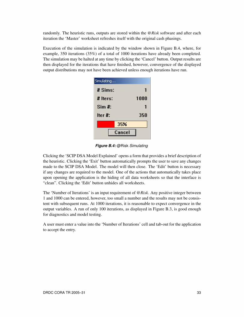
randomly. The heuristic runs, outputs are stored within the @Risk software and after eachiteration the ‘Master’ worksheet refreshes itself with the original cash phasings.
Execution of the simulation is indicated by the window shown in Figure B.4, where, forexample, 350 iterations (35%) of a total of 1000 iterations have already been completed.The simulation may be halted at any time by clicking the ‘Cancel’ button. Output results arethen displayed for the iterations that have finished, however, convergence of the displayedoutput distributions may not have been achieved unless enough iterations have run.
Figure B.4: @Risk Simulating
Clicking the ‘SCIP DSA Model Explained’ opens a form that provides a brief description ofthe heuristic. Clicking the ‘Exit’ button automatically prompts the user to save any changesmade to the SCIP DSA Model. The model will then close. The ‘Edit’ button is necessaryif any changes are required to the model. One of the actions that automatically takes placeupon opening the application is the hiding of all data worksheets so that the interface is“clean”. Clicking the ‘Edit’ button unhides all worksheets.
The ‘Number of Iterations’ is an input requirement of @Risk. Any positive integer between1 and 1000 can be entered, however, too small a number and the results may not be consis-tent with subsequent runs. At 1000 iterations, it is reasonable to expect convergence in theoutput variables. A run of only 100 iterations, as displayed in Figure B.3, is good enoughfor diagnostics and model testing.
A user must enter a value into the ‘Number of Iterations’ cell and tab-out for the applicationto accept the entry.
DRDC CORA TR 2005–31 33
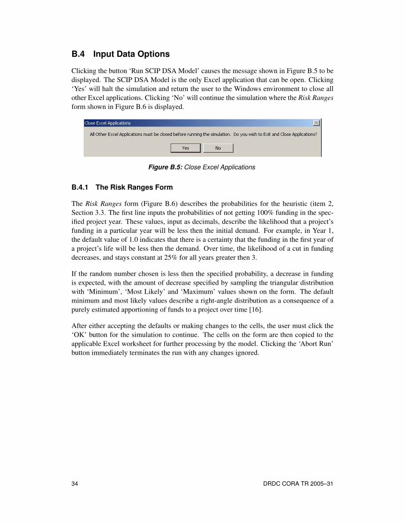
B.4 Input Data Options
Clicking the button ‘Run SCIP DSA Model’ causes the message shown in Figure B.5 to bedisplayed. The SCIP DSA Model is the only Excel application that can be open. Clicking‘Yes’ will halt the simulation and return the user to the Windows environment to close allother Excel applications. Clicking ‘No’ will continue the simulation where the Risk Rangesform shown in Figure B.6 is displayed.
Figure B.5: Close Excel Applications
B.4.1 The Risk Ranges Form
The Risk Ranges form (Figure B.6) describes the probabilities for the heuristic (item 2,Section 3.3. The first line inputs the probabilities of not getting 100% funding in the spec-ified project year. These values, input as decimals, describe the likelihood that a project’sfunding in a particular year will be less then the initial demand. For example, in Year 1,the default value of 1.0 indicates that there is a certainty that the funding in the first year ofa project’s life will be less then the demand. Over time, the likelihood of a cut in fundingdecreases, and stays constant at 25% for all years greater then 3.
If the random number chosen is less then the specified probability, a decrease in fundingis expected, with the amount of decrease specified by sampling the triangular distributionwith ‘Minimum’, ‘Most Likely’ and ‘Maximum’ values shown on the form. The defaultminimum and most likely values describe a right-angle distribution as a consequence of apurely estimated apportioning of funds to a project over time [16].
After either accepting the defaults or making changes to the cells, the user must click the‘OK’ button for the simulation to continue. The cells on the form are then copied to theapplicable Excel worksheet for further processing by the model. Clicking the ‘Abort Run’button immediately terminates the run with any changes ignored.
34 DRDC CORA TR 2005–31
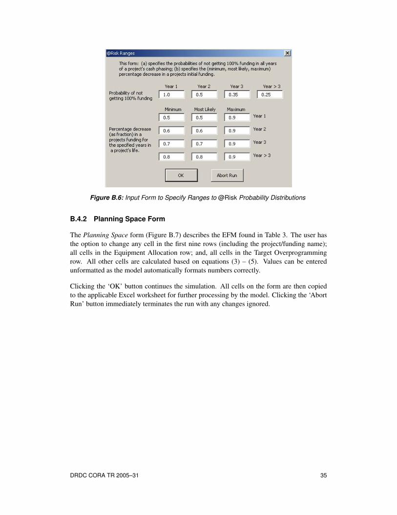
Figure B.6: Input Form to Specify Ranges to @Risk Probability Distributions
B.4.2 Planning Space Form
The Planning Space form (Figure B.7) describes the EFM found in Table 3. The user hasthe option to change any cell in the first nine rows (including the project/funding name);all cells in the Equipment Allocation row; and, all cells in the Target Overprogrammingrow. All other cells are calculated based on equations (3) – (5). Values can be enteredunformatted as the model automatically formats numbers correctly.
Clicking the ‘OK’ button continues the simulation. All cells on the form are then copiedto the applicable Excel worksheet for further processing by the model. Clicking the ‘AbortRun’ button immediately terminates the run with any changes ignored.
DRDC CORA TR 2005–31 35

Figu
reB
.7:I
nput
Form
toC
alcu
late
Free
Pla
nnin
gS
pace
36 DRDC CORA TR 2005–31

B.4.3 Adjust Start Date Form
The Adjust Start Date form allows the user to move a project’s entire cash phasing to theright or left from its initial position prior to running the model. It does this by shifting thefunds in the worksheet according to a new ‘Start FY’.
Figure B.8 shows the form containing the entire project list, which is loaded at start-upfrom the master Excel worksheet. There are two columns of information that are loaded:A Defence Services Program (DSP) number which labels the project as belonging to a par-ticular Level 1; and, the project title. The user then has two choices for finding a project inthe list, (a) they can either enter the first few characters of the DSP number, or (b) enter thefirst few characters of the project title. In either case, the algorithm starts selecting projectswith the first character entered and only stops when the search retrieves an unambiguousrecord. In the example shown, adding the character ‘r’ removed any ambiguity as there arethree projects that started with the characters ‘da’, i.e., ‘Data Link Modernization’, ‘DataManagement System Upgrade’ and ‘DART Upgrades’ (case is ignored). If characters areentered that don’t match any in the list, a message is displayed on the form stating ‘Projectis not in list’, at which point the user can either correct the text or select a project from thelist by using the scroll bar on the right or arrow keys on the keyboard.
Figure B.8: Input Form to Adjust Individual Project Start Dates
Once a project is selected, the ‘Start FY’ holds the initial start date and ‘End FY’ holdsthe initial completion data for the project with FY’s [1, 2, 3, . . .15, 16 ] equating to FY’s[05/06, 06/07, 07/08, . . .19/20, Future ] respectively. If the project is not funded, boththe ‘Start FY’ and ‘End FY’ boxes will have zeros entered and the message ‘Project is notfunded’ is displayed. If the project is funded, the user can adjust the start date by enteringa number in the ‘Start FY’ box. If the end date extends beyond the SCIP timeline, all costs
DRDC CORA TR 2005–31 37

beyond FY 19/20 are summed into the Future cell, i.e., in the example shown, the project‘DART Upgrades’ starts in FY 08/09 and has a duration of four years. Therefore, enteringa value of 14 in the ‘Start FY’ box will mean that cells ‘Future’ and ‘Future+1’ would besummed into the ‘Future’ cell.
Once the user tabs out of the ‘Start FY’ box, the changes are accepted by the model andonly by clicking the ‘Undo’ button could the changes be reversed. Clicking the ‘OK’ buttonwould exit the form and finalize any changes. Clicking the ‘Abort Run’ button would alsoreverse any changes prior to terminating the run.
B.5 Error Checking
Throughout the user entry portions of the model, errors in the data entry are automaticallyflagged for the user to take corrective action.
B.5.1 Main Menu Error Checking
Such is the case with the ‘Number of Iterations’ on the ‘Main Menu’ sheet (Figure B.3).The user must enter a value in the cell and tab-out of the cell for the application to acceptthe entry. If zero, a negative value or a value greater than 1000 is entered, a message asshown in Figure B.9 is displayed and the user is returned to the worksheet to correct theentry.
Figure B.9: Message for Invalid Entry in ‘Number of Iterations’ Cell
B.5.2 Risk Ranges Form Error Checking
All entries in the ‘Risk Ranges’ form are probability values that are critical to the successfulrunning of the heuristic. Invalid entries occur when the user either enters a non-numericor negative character, a probability greater than one or specifies an invalid range for thetriangular distribution.
When a value is entered, the model first checks to make sure it is numeric. If it is non-numeric, the message in Figure B.10 is displayed and the user is returned to the textboxin question for correction. Until a numeric value is entered, the model will not relinquishcontrol to the user. Similarly, if a non-negative probability is entered, the message in FigureB.11 is displayed and the user is returned to the textbox in question for correction. Until apositive value is entered, the model will not relinquish control to the user.
38 DRDC CORA TR 2005–31

Figure B.10: Message for Non Numeric Entry Figure B.11: Message for Non NegativeEntry
The model also checks for “correctness” in probabilities. If a probability greater then 1.0is entered, the message in Figure B.12 is displayed and the user is returned to the textboxin question for correction. Until a value less then one is entered, the model will not re-linquish control to the user. Also, for the three values required to define the range of thetriangular distribution, if the range: [Minimum ≤ Most Likely ≤ Maximum ] is violated,the message in Figure B.13 is displayed and the user is returned to the textbox in questionfor correction.
Figure B.12: Message for ProbabilityLimit Error
Figure B.13: Message for Bad Range forTriangular Distribution
B.5.3 Planning Space Form Error Checking
The Planning Space form requires a variety of number formats that are automatically ad-justed to suit the particular format of the cell. Entering a number in the percentage cell willautomatically reformat the number as a percentage. Similarly, a blank entry is replaced bya ‘0’ and any number greater than 999 is automatically formatted with a ‘,’ as the 1000separator.
B.5.4 Adjust Start Date Form Error Checking
The Adjust Start Date form takes its input directly from the master Excel worksheet thatlists the prioritized SCIP projects. If a user enter a DSP Number or Project Title that is notin the list, a message stating ‘Project is Not in List’ is displayed in red directly on the form.The user can then either correct the mistake or manually select a project from the list.
When entering the ‘Start FY’ number, there are two tests that the entry undergoes:
• If a non-numeric character is entered, a message as in Figure B.10 is displayed andcontrol is returned to the user for correction;
DRDC CORA TR 2005–31 39

• If a negative number is entered, a message as in Figure B.11 is displayed and control isreturned to the user for correction.
B.5.5 @Risk Error Checking
The VBA code developed for the SCIP DSA Model uses public @Risk variables and func-tions to facilitate the simulation. The function ‘RiskSetSettings’, for example, is used toset the simulation to the current @Risk settings. The return value of the function is zero ifthe call is successful. If the return value is non-zero, an error has occurred and the valueis passed to the ‘RiskError’ function to get a description and location of the error. FigureB.14 is an example of an error generated through the ‘RiskSetSettings’ function. Clickingthe ‘OK’ button aborts the simulation.
Figure B.14: Error Generated at RiskSetSettings
Other @Risk error checking occurs within the functions ‘RiskGetSettings’, ‘RiskGener-ateReports’ and ‘RiskSimulate’.
B.5.6 Office 2000 Error Checking
The SCIP DSA Model is designed to work with Excel 2000 or later. Should the user try torun the application from an earlier version, the message displayed in Figure B.15 is shownand the workbook is closed.
Figure B.15: Office 2000 Check
40 DRDC CORA TR 2005–31

List of symbols/abbreviations/acronyms/initialisms
ADM(HR Mil) Assistant Deputy Minister(Human Resources–Military)ADM(IM) Assistant Deputy Minister(Information Management)ADM(Pol) Assistant Deputy Minister(Policy)ADM(S&T) Assistant Deputy Minister(Science and Technology)CF Canadian ForcesCAS Chief of the Air StaffCDS Chief of the Defence StaffCLS Chief of the Land StaffCMS Chief of the Maritime StaffDCDS Deputy Chief of the Defence StaffDFPPC Director Force Planning and Program CoordinationDM Deputy MinisterDND Department of National DefenceDRDC Defence Research and Development CanadaDSA Decision Support AnalysisDSP Defence Services ProgramEFM Equipment Funding MatrixFY Fiscal YearIM Information ManagementIT Information TechnologyJCRB Joint Capability Requirement BoardMARCUS Multi-Criteria Analysis and Ranking Consensus Unified SolutionO&M Operations and MaintenancePFM Project Funding MatrixPMB Program Management BoardSCIP Strategic Capability Investment PlanTri TriangularVBA Visual Basic for ApplicationsWG Working Group
DRDC CORA TR 2005–31 41

This page intentionally left blank.
42 DRDC CORA TR 2005–31

DOCUMENT CONTROL DATA(Security classification of title, body of abstract and indexing annotation must be entered when document is classified)
1. ORIGINATOR (the name and address of the organization preparing the document.Organizations for whom the document was prepared, e.g. Centre sponsoring acontractor’s report, or tasking agency, are entered in section 8.)
DRDC – Centre for Operational Research and AnalysisNDHQ, 101 Col By Drive, Ottawa ON K1A 0K2
2. SECURITY CLASSIFICATION(overall security classification of the documentincluding special warning terms if applicable).
UNCLASSIFIED
3. TITLE (the complete document title as indicated on the title page. Its classification should be indicated by the appropriateabbreviation (S,C,R or U) in parentheses after the title).
The Strategic Capability Investment Plan Decision Support Analysis Model
4. AUTHORS(Last name, first name, middle initial. If military, show rank, e.g. Doe, Maj. John E.)
Desmier, P.E.
5. DATE OF PUBLICATION (month and year of publication of document)
November 2005
6a. NO. OF PAGES (totalcontaining information. IncludeAnnexes, Appendices, etc).
56
6b. NO. OF REFS (total cited indocument)
16
7. DESCRIPTIVE NOTES (the category of the document, e.g. technical report, technical note or memorandum. If appropriate, enter the type of report,e.g. interim, progress, summary, annual or final. Give the inclusive dates when a specific reporting period is covered).
Technical Report
8. SPONSORING ACTIVITY (the name of the department project office or laboratory sponsoring the research and development. Include address).
DRDC – Centre for Operational Research and AnalysisNDHQ, 101 Col By Drive, Ottawa ON K1A 0K2
9a. PROJECT OR GRANT NO. (if appropriate, the applicable research anddevelopment project or grant number under which the document waswritten. Specify whether project or grant).
9b. CONTRACT NO. (if appropriate, the applicable number under whichthe document was written).
10a. ORIGINATOR’S DOCUMENT NUMBER (the official document numberby which the document is identified by the originating activity. Thisnumber must be unique.)
DRDC CORA TR 2005–31
10b. OTHER DOCUMENT NOs. (Any other numbers which may beassigned this document either by the originator or by the sponsor.)
11. DOCUMENT AVAILABILITY (any limitations on further dissemination of the document, other than those imposed by security classification)
( X ) Unlimited distribution( ) Defence departments and defence contractors; further distribution only as approved( ) Defence departments and Canadian defence contractors; further distribution only as approved( ) Government departments and agencies; further distribution only as approved( ) Defence departments; further distribution only as approved( ) Other (please specify):
12. DOCUMENT ANNOUNCEMENT (any limitation to the bibliographic announcement of this document. This will normally correspond to the DocumentAvailability (11). However, where further distribution beyond the audience specified in (11) is possible, a wider announcement audience may beselected).

13. ABSTRACT (a brief and factual summary of the document. It may also appear elsewhere in the body of the document itself. It is highly desirable that theabstract of classified documents be unclassified. Each paragraph of the abstract shall begin with an indication of the security classification of theinformation in the paragraph (unless the document itself is unclassified) represented as (S), (C), (R), or (U). It is not necessary to include here abstracts inboth official languages unless the text is bilingual).
Updating the SCIP equipment annex for C Status and below projects is an annual process that consumesa great deal of staff time and resources. This report documents a model that strives to bring the rigor ofcomputer simulation, risk analysis and optimization into the SCIP process. It easily lends itself to ‘Whatif’ type analyses through varying the input funding, the likelihood of a decrease in funding, the range of apossible decrease and adjustments to project start dates.
The model, once implemented, will support a more sophisticated and rigorous approach to planning andprioritizing future strategic capital (equipment) projects and, it is foreseen, form the nucleus of three distinctbut related decision support analysis models where the output from an A and B capital equipment futurespending model is used as input to the SCIP decision support model described herein. Its output in turnwould be used as an input to a third, future O&M decision support model to determine the impact on futureO&M budgets from approving and implementing the SCIP projects.
14. KEYWORDS, DESCRIPTORS or IDENTIFIERS (technically meaningful terms or short phrases that characterize a document and could be helpful incataloguing the document. They should be selected so that no security classification is required. Identifiers, such as equipment model designation, tradename, military project code name, geographic location may also be included. If possible keywords should be selected from a published thesaurus. e.g.Thesaurus of Engineering and Scientific Terms (TEST) and that thesaurus-identified. If it not possible to select indexing terms which are Unclassified, theclassification of each should be indicated as with the title).
SCIPStrategicCapabilityInvestmentCapitalO&MEquipmentOverprogrammingUnderprogrammingMonte CarloSimulationTriangular DistributionMARCUSSliceHeuristicPrioritizeRankingProjects


DRDC CORA
www.drdc-rddc.gc.ca