The State of the Art in Flow Visualization: Dense and Texture-Based ...

Volume 23 (2004), number 2 pp. 203–221 COMPUTER GRAPHICS forum

The State of the Art in Flow Visualization: Denseand Texture-Based Techniques

Robert S. Laramee,1 Helwig Hauser,1 Helmut Doleisch,1 Benjamin Vrolijk,2 Frits H. Post2 and Daniel Weiskopf3

1 VRVis Research Center, Austria2 Delft University of Technology, Netherlands

3 VIS, University of Stuttgart, Germany

AbstractFlow visualization has been a very attractive component of scientific visualization research for a long time.Usually very large multivariate datasets require processing. These datasets often consist of a large number ofsample locations and several time steps. The steadily increasing performance of computers has recently becomea driving factor for a reemergence in flow visualization research, especially in texture-based techniques. In thispaper, dense, texture-based flow visualization techniques are discussed. This class of techniques attempts to providea complete, dense representation of the flow field with high spatio-temporal coherency. An attempt of categorizingclosely related solutions is incorporated and presented. Fundamentals are shortly addressed as well as advantagesand disadvantages of the methods.

Keywords: visualization, flow visualization, vector field visualization, texture-based flow visualization.

ACM CCS: I.3 [Computer Graphics]: visualization, flow visualization, computational flow visualization

1. Introduction

Flow visualization (FlowVis) is one of the classic subfieldsof visualization, covering a rich variety of applications, fromthe automotive industry, aerodynamics, turbomachinery de-sign, to weather simulation, meteorology, climate modeling,ground water flow and medical visualization. Consequently,the spectrum of FlowVis solutions is very rich, spanning mul-tiple technical challenges: 2D versus 3D solutions and tech-niques for steady or time-dependent data.

Bringing many of those solutions in linear order (as neces-sary for a text like this) is neither easy nor intuitive. Severaloptions of subdividing this broad field of literature are pos-sible. Hesselink et al., for example, addressed the problemof how to categorize techniques in their 1994 overview ofresearch issues [24] and consider dimensionality as a meansto classify the literature. In the following, several aspects arediscussed on an abstract level before literature is addresseddirectly.

1.1. Classification

According to the different needs of the users, there are dif-ferent approaches to flow visualization (cf. Figure 1):� Direct flow visualization: This category of techniques

uses a translation that is as direct as possible for repre-senting flow data in the resulting visualization. The resultis an overall picture of the flow. Common approaches aredrawing arrows (Figure 2, left) or color coding velocity.Intuitive pictures can be provided, especially in the caseof two dimensions. Solutions of this kind allow immedi-ate investigation of the flow data.

� Dense, texture-based flow visualization: Similar to directflow visualization, a texture is computed that is used togenerate a dense representation of the flow (Figure 2,middle). A notion of where the flow moves is incorpo-rated through corelated texture values along the vectorfield. In most cases this effect is achieved through filter-ing of texture values according to the local flow vector.

c© The Eurographics Association and Blackwell Publishing Ltd2004. Published by Blackwell Publishing, 9600 GarsingtonRoad, Oxford OX4 2DQ, UK and 350 Main Street, Malden,MA 02148, USA. 203

Submitted December 2002Revised February 2003Accepted March 2004

204 R. S. Laramee et al. /Flow Visualization: Dense and Texture-Based Techniques

Figure 1: Classification of flow visualization techniques—(left) direct, (middle-left) texture-based, (middle-right) basedon geometric objects and (right) feature-based.

� Geometric flow visualization: For a better communica-tion of the long-term behavior induced by flow dynam-ics, integration-based approaches first integrate the flowdata and use geometric objects as a basis for flow visu-alization. The resulting integral objects have a geometrythat reflects the properties of the flow. Examples includestreamlines (Figure 2, right), streaklines and pathlines.These geometric objects are based on integration as op-posed to other geometric objects, like isosurfaces, thatmay also be useful for visualization. A description ofgeometric techniques is presented by Post et al. [55].

� Feature-based flow visualization: Another approachmakes use of an abstraction and/or extraction step whichis performed before visualization. Special features are ex-tracted from the original dataset, such as important phe-nomena or topological information of the flow. Visual-ization is then based on these flow features (instead of theentire dataset), allowing for compact and efficient flowvisualization, even of very large and/or time-dependentdatasets. This can also be thought of as visualization ofderived data. Post et al. [56] cover feature-based flowvisualization in detail.

Figure 1 illustrates a classification of the aforementionedclasses and Figure 2 shows three typical examples. Notethat there are different amounts of computation associatedwith each category. In general, direct flow visualization tech-niques require less computation than the other three cate-gories, whereas feature-based techniques require the mostcomputation. This overview focuses on the body of researchrelated to dense, texture-based techniques.

1.2. Spatial temporal and data dimensionality

Solutions in flow visualization differ with respect to the di-mensionality of the flow data. Useful techniques for 2D flowdata, like color coding or arrow plots, sometimes lack similaradvantages in 3D. Here, the spatial dimensionality of the flowdata is indicated as either 2D, 2.5D or 3D. In our classifica-tion the dimensionality of the results from each technique is

marked with a corresponding label indicating dimensionality(see Figure 4).

By 2.5D we mean flow visualization restricted to surfacesin 3D. We draw attention to the notion that in many caseslike CFD, the simulation sets all velocities on a surface tozero. One way to approach this is to extrapolate the vectorfield just inside the surface to the boundary. In any case, thevector component normal to the surface is usually lost inthe visualization. Furthermore, another vector field can becalculated on a surface, such as skin friction.

In addition to spatial dimension, temporal dimension (di-mensionality with respect to time) is of great importance.Firstly, velocity incorporates a notion of time—flows are of-ten interpreted as differential data with respect to time (cf.Equation 1), i.e. when integrating the data, instantaneouspaths such as streamlines may be obtained (cf. Equation 3).We call this steady velocity time. Additionally, the flow dataitself can change over time resulting in time-dependent (orunsteady) flow. We refer to this as unsteady velocity time.The visualization must carefully distinguish between both.Performing integration in the case of unsteady data results inpathlines or streaklines as opposed to streamlines.

The distinction between steady and unsteady velocity timeis important especially when animation is used in the visu-alization. Then, even a third notion of time, i.e. animationtime, may affect the visualization. Animation time can be anarbitrary feature added to the visualization in order to createmotion. Sometimes, geometric objects like streamlines areanimated in order to show flow orientation, e.g. the motionof color controlled by a color table [31]. Animation is alsooften added to texture-based methods with the same goal inmind. Special attention is required for correct interpretationof animation time.

In many cases, further data dimensions, i.e. attributes aresupplied with the data, such as temperature, pressure or vor-ticity in addition to spatial and temporal dimensions. Thedimension of the data values is also associated with the termsmultivariate and multi-field data. Flow visualization may alsotake these values into account, e.g. by using color or isosur-face extraction.

Although we do not have space to focus on experimen-tal flow visualization, it is interesting to recognize that manycomputational solutions more or less mimic the visual appear-ance of well-accepted techniques in experimental visualiza-tion (cf. particle traces, dye injection or Schlieren techniques[77]).

1.3. Data sources

Computational flow visualization, in general, deals with datathat exhibits temporal dynamics like the results from (a)flow simulation (e.g. the simulation of fluid flow through aturbine), (b) flow measurements (possibly acquired through

c© The Eurographics Association and Blackwell Publishing Ltd 2004

R. S. Laramee et al. /Flow Visualization: Dense and Texture-Based Techniques 205

Figure 2: An example of circular flow at the surface of a ring to help illustrate our flow visualization classification: (left) directvisualization by the use of arrow glyphs, (middle) texture-based by the use of LIC and (right) visualization based on geometricobjects, here streamlines.

laser-based technology) or (c) analytic models of flows (e.g.dynamical systems [1], given as set of differential equations).

We focus on visualization of data from computational flowsimulation, i.e. flow data given as a set of samples on a grid.In many cases, the velocity information in a flow dataset(encoded as a set of velocity vectors) represents the focus.Therefore, flow visualization is strongly related to vector fieldvisualization, which may also deal with vector fields otherthan velocity fields.

The relation of computational and experimental visualiza-tion is worthy of mention. Experimental flow visualization,as in a wind tunnel, is also used to validate computationalflow simulation. In such a case the computational visualiza-tion needs to be set up in a way such that results can be easilycompared.

2. Fundamentals

Before outlining some of the most important texture-basedtechniques, a short overview of common mathematics as wellas some general concepts with regard to the computation ofresults are presented.

Flow simulations are often solutions to systems of PDEs,such as the Navier Stokes, Euler or Advection-Diffusionequations [82]. In general, discretized solution methods areused. Noteworthy are finite volume (FV) and finite element(FE) analysis, which subdivide the domain into small ele-ments like hexahedral or tetrahedral cells. A solution is de-fined on the computation grid in physical space: unstructuredfor FE and structured curvilinear for FV solutions. In the dis-cussion that follows, we assume that vector data are definedon the grid nodes (cell vertices).

2.1. Reconstruction of flow data

An inherent characteristic of flow data is that derivative in-formation is given with respect to time, which is laid out with

respect to an n-dimensional spatial domain � ⊆ Rn, e.g. n =3 for representing 3D fluid flow. Temporal derivatives v ofnD locations p within the flow domain � are n-dimensionalvectors:

v = dp/dt, p ∈ � ⊆ Rn, v ∈ Rn, t ∈ R. (1)

A general formulation of (possibly unsteady) flow data v is

v(p, t) : � × � → Rn, (2)

where p ∈ � ⊆ Rn represents the spatial reference of the flowdata and t ∈ � ⊆ R represents the system time. For steadyflow data, the simpler case of v(p) : � → Rn is given (v notdependent on t).

In results from nD flow simulation, such as from automo-tive applications or airplane design, vector data v is usuallynot given in analytic form, but requires reconstruction fromthe discrete simulation output. The numerical methods usedfor the flow simulation, such as finite element methods, out-put simulation values usually on large-sized grids of manysample vectors vi, which discretely represent the solution ofthe simulation process. Furthermore, it is assumed that theflow simulation is based on a continuous model of the flowallowing continuous reconstruction of the flow data v. Oneoption is to apply a reconstruction filter h : Rn → R to com-pute v(p) = ∑

i h(p − pi )vi . For practical reasons, filter husually has only local extent. Efficient procedures for findingflow samples vi, which are nearest to the query point p, areneeded to do proper reconstruction.

2.2. Grids

In flow simulation, the vector samples vi usually are laidout across the flow domain with respect to a certain type ofgrid. Grid types range from simple rectilinear or Cartesiangrids to curvilinear grids to complex unstructured grids (cf.Figure 3). Typically, simulation grids exhibit large variationsin cell sizes. This variety of cell sizes stems from the influence



Figure 3: Grids involved in flow simulation—(a) Carte-sian, (b) regular, (c) general rectilinear, (d) structured orcurvilinear, (c) unstructured and (f) unstructured triangular[37,89].

of grid generation onto the flow simulation process. The qual-ity of the grid model and its implementation impact the qual-ity of the simulation results.

Although the principal theory of reconstruction from dis-crete samples does not exhibit many differences with respectto grid cell types, the practical handling does. While neigh-bor searching might be trivial in a rectilinear grid, it usuallyis not in a tetrahedral grid. Similar differences hold for theproblems of point location and vector reconstruction. In thefollowing we shortly describe some fundamental operationswhich form the basis for visualization computations on sim-ulation grids.

Starting with point location, i.e. the problem of finding thegrid cell in which a given nD-point lies, usually two casesare distinguished. For general point location, special datastructures can be used that subdivide the spatial domain tospeed up the search. For iterative point location, often neededduring integral curve computation, algorithms are used thatefficiently exploit spatial coherence during the search. Onekind of such algorithms starts with an initial guess for thetarget cell, checks for point containment and refines accord-ingly afterward. This process is iterated until the target cellis found. More details can be found in text books about flowvisualization fundamentals [53,68].

Beside point location, flow reconstruction, or interpola-tion, within a cell of the dataset is a crucial issue. Often,once the cell containing the query location is found, onlythe sample vectors at the cell’s vertices are considered forreconstruction. The approach used most often is first-orderreconstruction by performing linear interpolation within thecell. For example, trilinear flow reconstruction may be usedwithin a 3D hexahedral cell.

After point location and flow reconstruction, visualizationbegins: vectors can be represented with glyphs; virtual parti-cles can be injected and traced across the flow domain. Nev-ertheless, the computation of derived data may be necessaryto do more sophisticated flow visualization. Usually, the firststep is to request second-order gradient information for arbi-trary points in the flow domain, i.e. ∇v|p, which gives infor-mation about local properties of the flow (at point p) such asflow convergence and divergence, or flow rotation and shear.For feature extraction, flow vorticity ω = ∇ × v can be ofhigh interest. Further details about local flow properties canbe found in previous work [45,54].

2.3. Integration

Recalling that flow data in most cases is derivative informa-tion with respect to time, the idea of integrating flow data overtime is natural to provide an intuitive notion of evolution in-duced by the flow. One example is visualization by the useof particle advection. A respective particle path p(t)—herethrough unsteady flow—can be defined by

p(t) = p0 +∫ t

τ=0v(p(τ ), τ ) dτ, (3)

where p0 represents the location of the particle path at seedtime 0. Note that Equations 1 and 3 are complimentary to eachother. For other types of integral curves, such as streaklinessee previous work [36,68].

In addition to the theoretical specification of integralcurves, it is important to note that respective integral equa-tions like Equation 3 usually cannot be resolved for thecurve function analytically, and thereby numerical integra-tion methods are employed. The most simple approach is touse a first-order Euler method to compute an approximationpE(t)—one iteration of the curve integration is specified by

pE (t + t) = p(t) + t · v(p(t), t), (4)

where t usually is a very small step in time and p(t) denotesthe location to start this Euler step from. A more accurate butalso more costly technique is the second-order Runge-Kuttamethod [57], which uses the Euler approximation pE as alook-ahead to compute a better approximation pRK2(t) of theintegral curve:

pRK 2(t + t) = p(t) + t · (v(p(t), t)

+ v(pE (t + t), t))/2. (5)

Higher-order methods like the often used fourth-order Runge-Kutta integrator utilize more such steps to better approximatethe local behavior of the integral curve. Also, adaptive stepsizes are used to compute smaller steps in regions of highcurvature.



3. Dense and Texture-Based Flow Visualization

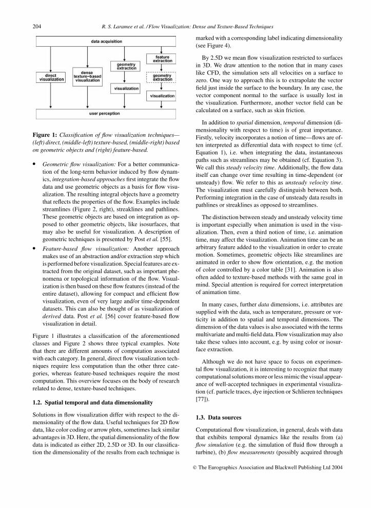
Dense, texture-based techniques in flow visualization gener-ally provide full spatial coverage of the vector field. In ourclassification we group these methods into the following cat-egories based on their respective primitive: the fundamentalobject upon which the algorithm is based. Our classificationsubdivides the techniques based on their similarity.

� Spot Noise techniques: These methods (Section 3.1) arebased on a technique introduced by Van Wijk [78]. In thiscategory, the basic primitive on which the algorithms op-erate is the so-called spot: an ellipse or other shape thatis warped and distributed in order to reflect the charac-teristics of a vector field.

� LIC techniques: The methods in this category (Sec-tion 3.2) are derived from an algorithm introduced byCabral and Leedom [8], namely, line integral convolution(LIC). The basic primitive here is a noise texture: theproperties of texture are convolved, or smeared, using akernel filter in the direction of the underlying vector field.

� Texture advection and GPU-based techniques: The prim-itive in this case (Section 3.3) is a moving texel [50]. In-dividual texels/texel properties, or groups of texels areadvected in the direction of the vector field. Many ofthe techniques in this category utilize more computationon the GPU (Graphics Processing Unit)—rather than theCPU—in order to realize performance gains.

� Related techniques: Most of the dense, texture-basedflow visualization research falls into one of the previ-ous categories. Related research that does not fit cleanlyinto one of the previous classifications is discussed inSection 3.4.

We have included a section of meta-research papers in Sec-tion 4 after the individual research techniques. These papersattempt to provide an alternative, higher-level framework thatincorporates many of the techniques discussed here.

3.1. Spot noise

Spot noise, introduced by Van Wijk [78], was one of the firstdense, texture-based techniques for vector field visualization.Spot noise generates a texture by distributing a set of intensityfunctions, or spots, over the domain. Each spot represents aparticle warped over a small step in time and results in a streakin the direction of the local flow from where the particle isseeded. A spot noise texture is defined by: [78]

f (x) =∑

ai h(x − xi , v(xi )) (6)

in which h( ) is called the intensity function, ai is a scalingfactor, and xi is a random position. A spot is a function withunity intensity value for the spot, e.g. a ellipse and its inte-rior, and zero everywhere else. The summation denotes the

Figure 4: The spot noise hierarchy of related research. Chil-dren in the hierarchy build upon the work of their parent.

Figure 5: A snapshot of the unsteady spot noise algorithm[16]. Image courtesy of De Leeuw and Van Liere.

blending of each instance of the intensity function at randompositions.

The hierarchy shown in Figure 4 illustrates the relationshipamongst spot noise related methods. Follow-up research thatbuilds upon a previous technique is shown as a child in thehierarchy. Children that share a common parent are presentedin chronological order of appearance when reading from leftto right. Each node in the hierarchy is labeled and the corre-sponding description can be matched in the text of this article.The dimensionality of the flow data used to generate the re-sults is indicated for convenience. The time dimension labelis given a different shape to distinguish it from the spatialdimensions. We believe the spot noise hierarchy (Figure 4)and the LIC hierarchy (Figure 7) will be valuable assets inhelping the reader navigate the related research literature. Inwhat follows, we visit each node in the hierarchy in depth-first-search order.

Comparative visualization: Spot noise has been used to sim-ulate the results from the field of experimental flow visual-ization [14]. First, the parameters of the spot noise techniqueare tuned in order to simulate the smearing of oil on a surface.A postprocessing step is then added to enhance the visual-ization result such that it looks closer to the smearing of realoil from experimental flow visualization.



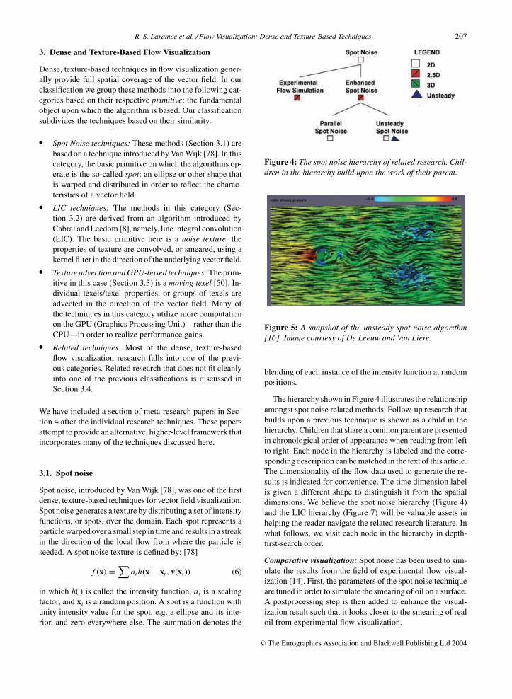
Figure 6: Visualization of flow past a box using (left) spot noise and (right) LIC.

Enhanced spot noise: One limitation of the original spotnoise algorithm was the inability to represent high, local ve-locity curvature especially with high speeds. Enhanced spotnoise [12] by De Leeuw and Van Wijk addresses these chal-lenges through the use of bent spot primitives.

Parallel and unsteady spot noise: In order to acceleratethe performance of enhanced spot noise towards interactiveframe rates, a parallel implementation of the algorithm wasintroduced by De Leeuw [13]. The parallel implementationwas applied to the steering of a smog prediction simulationand searching a very large data set resulting from a numericalsimulation of turbulence.

The first application of spot noise to unsteady flow is pre-sented by De Leeuw and Van Liere [16] (Figure 5). Themotion of spots is modeled after particles in unsteady flow.In order to visualize unsteady flow, the distribution of spotswith respect to the temporal domain is discussed. Unsteadyspot noise also introduces support for zooming views of thevector field. Spot noise with zooming is also utilized by DeLeeuw and Van Liere when visualizing topological featuresof 2D flow [10].

Spot noise related literature: A combination of both texture-based FlowVis on 2D slices and 3D arrows for 3D flow vi-sualization is employed by Telea and Van Wijk [74]. Arrowsdenote the main characteristics of the 3D flow after clusteringand a 2D slice with spot noise visualization serves as context.The focus of this work is on vector field clustering.

Loffelmann et al. [44] use anisotropic spot noise createdfrom a grid-shaped spot to visualize streamlines and timelinesconcurrently on stream surfaces. Another interesting appli-

cation of spot noise is its use for the depiction of discretemaps (noncontinuous flow) [43].

Spot noise has also been applied to the visualization ofturbulent flow [15] and in combination with the visualizationof flow topology [10,11]. We refer the reader to Post et al.[55,56] for more on the subject of flow topology.

Spot noise versus LIC: A visual comparison of LIC (thefocus of the next section) and spot noise is shown in Figure 6.Spot noise is capable of reflecting velocity magnitude withinthe amount of smearing in the texture, thus freeing up huefor the visualization of another attribute such as pressure,temperature, etc. On the other hand, LIC is more suited forthe visualization of critical points which is a key elementin conveying the flow topology. The vector magnitudes arenormalized thus retaining lower spatial frequency texture inareas of low velocity magnitude. De Leeuw and Van Lierealso compare spot noise to LIC [17]. They report that LICis better at showing direction than spot noise, but it does notencode velocity magnitude. By flow direction, we refer to thepath along which a massless particle follows when injectedinto the flow.

3.2. Line integral convolution

Line integral convolution (LIC), first introduced by Cabraland Leedom [8], has spawned a large collection of research asindicated in Figure 7. The original LIC method takes as inputa vector field on a 2D, Cartesian grid and a white noise textureof the same size. Texels are convolved (or correlated) alongthe path of streamlines using a filter kernel in order to create adense visualization of the flow field. More specifically, givena streamline σ, LIC consists of calculating the intensity I for



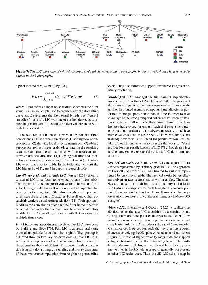
Figure 7: The LIC hierarchy of related research. Node labels correspond to paragraphs in the text, which then lead to specificentries in the bibliography.

a pixel located at x0 = σ(s 0) by: [70]

I (x0) =∫ s0+L/2

s0−L/2k(s − s0)T (σ(s)) ds (7)

where T stands for an input noise texture, k denotes the filterkernel, s is an arc length used to parameterize the streamlinecurve and L represents the filter kernel length. See Figure 2(middle) for a result. LIC was one of the first dense, texture-based algorithms able to accurately reflect velocity fields withhigh local curvature.

The research in LIC-based flow visualization describedhere extends LIC in several directions: (1) adding flow orien-tation cues, (2) showing local velocity magnitude, (3) addingsupport for nonrectilinear grids, (4) animating the resultingtextures such that the animation shows the upstream anddownstream flow direction, (4) allowing real-time and inter-active exploration, (5) extending LIC to 3D and (6) extendingLIC to unsteady vector fields. In the following, we visit theLIC hierarchy of Figure 7 in depth-first-search order.

Curvilinear grids and unsteady LIC: Forssell [20] was earlyto extend LIC to surfaces represented by curvilinear grids.The original LIC method portrays a vector field with uniformvelocity magnitude. Forssell introduces a technique for dis-playing vector magnitude. She also describes one approachto animate the resulting LIC textures. Forssell and Cohen ex-tend this work to visualize unsteady flow [21]. Their approachmodifies the convolution such that the filter kernel operateson streaklines rather than streamlines. In other words, theymodify the LIC algorithm to trace a path that incorporatesmultiple time steps.

Fast LIC: Many algorithms are built on fast LIC introducedby Stalling and Hege [70]. Fast LIC is approximately oneorder of magnitude faster than the original. The speedup isachieved through two key observations: (1) fast LIC min-imizes the computation of redundant streamlines present inthe original method and (2) fast LIC exploits similar convolu-tion integrals along a single streamline and thus re-uses partsof the convolution computation from neighboring streamline

texels. They also introduce support for filtered images at ar-bitrary resolution.

Parallel fast LIC: Amongst the first parallel implementa-tions of fast LIC is that of Zockler et al. [90]. The proposedalgorithm computes animation sequences on a massivelyparallel distributed memory computer. Parallelization is per-formed in image space rather than in time in order to takeadvantage of the strong temporal coherence between frames.Luckily, as we shall see later, flow visualization research inthis area has evolved far enough such that expensive paral-lel processing hardware is not always necessary to achieveinteractive visualization [28,29,38,79]. However, for 3D andunsteady flow there is still need for parallelization. For thesake of completeness, we also mention the work of Cabraland Leedom on parallelization of LIC [7] although this is aparallel processing version of the original LIC algorithm, notfast LIC.

Fast LIC on surfaces: Battke et al. [2] extend fast LIC tosurfaces represented by arbitrary grids in 3D. The approachby Forssell and Cohen [21] was limited to surfaces repre-sented by curvilinear grids. The method works by tessellat-ing a given surface representation with triangles. The trian-gles are packed (or tiled) into texture memory and a localLIC texture is computed for each triangle. The results pre-sented here are limited to relatively small simple surface rep-resentations composed of equilateral triangles (1,600–4,000triangles).

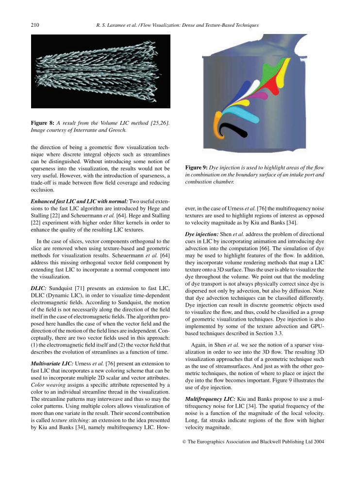
Volume LIC: Interrante and Grosch [25,26] visualize true3D flow using the fast LIC algorithm as a starting point.Clearly, there are perceptual challenges related to 3D flowvisualization such as occlusion, depth perception and visualcomplexity. Volume LIC introduces the use of halos in orderto enhance depth perception such that the user has a betterchance at perceiving the 3D space covered in the visualization(Figure 8). Areas of higher velocity magnitude are mappedto higher texture opacity. It is interesting to note that withthe introduction of halos, we are then able to identify dis-tinct entities in the 3D field, a property generally not presentin other LIC techniques. Thus, the 3D LIC takes a step in



Figure 8: A result from the Volume LIC method [25,26].Image courtesy of Interrante and Grosch.

the direction of being a geometric flow visualization tech-nique where discrete integral objects such as streamlinescan be distinguished. Without introducing some notion ofsparseness into the visualization, the results would not bevery useful. However, with the introduction of sparseness, atrade-off is made between flow field coverage and reducingocclusion.

Enhanced fast LIC and LIC with normal: Two useful exten-sions to the fast LIC algorithm are introduced by Hege andStalling [22] and Scheuermann et al. [64]. Hege and Stalling[22] experiment with higher order filter kernels in order toenhance the quality of the resulting LIC textures.

In the case of slices, vector components orthogonal to theslice are removed when using texture-based and geometricmethods for visualization results. Scheuermann et al. [64]address this missing orthogonal vector field component byextending fast LIC to incorporate a normal component intothe visualization.

DLIC: Sundquist [71] presents an extension to fast LIC,DLIC (Dynamic LIC), in order to visualize time-dependentelectromagnetic fields. According to Sundquist, the motionof the field is not necessarily along the direction of the fielditself in the case of electromagnetic fields. The algorithm pro-posed here handles the case of when the vector field and thedirection of the motion of the field lines are independent. Con-ceptually, there are two vector fields used in this approach:(1) the electromagnetic field itself and (2) the vector field thatdescribes the evolution of streamlines as a function of time.

Multivariate LIC: Urness et al. [76] present an extension tofast LIC that incorporates a new coloring scheme that can beused to incorporate multiple 2D scalar and vector attributes.Color weaving assigns a specific attribute represented by acolor to an individual streamline thread in the visualization.The streamline patterns may interweave and thus so may thecolor patterns. Using multiple colors allows visualization ofmore than one variate in the result. Their second contributionis called texture stitching: an extension to the idea presentedby Kiu and Banks [34], namely multifrequency LIC. How-

Figure 9: Dye injection is used to highlight areas of the flowin combination on the boundary surface of an intake port andcombustion chamber.

ever, in the case of Urness et al. [76] the multifrequency noisetextures are used to highlight regions of interest as opposedto velocity magnitude as by Kiu and Banks [34].

Dye injection: Shen et al. address the problem of directionalcues in LIC by incorporating animation and introducing dyeadvection into the computation [66]. The simulation of dyemay be used to highlight features of the flow. In addition,they incorporate volume rendering methods that map a LICtexture onto a 3D surface. Thus the user is able to visualize thedye throughout the volume. We point out that the modelingof dye transport is not always physically correct since dye isdispersed not only by advection, but also by diffusion. Notethat dye advection techniques can be classified differently.Dye injection can result in discrete geometric objects usedto visualize the flow, and thus, could be classified as a groupof geometric visualization techniques. Dye injection is alsoimplemented by some of the texture advection and GPU-based techniques described in Section 3.3.

Again, in Shen et al. we see the notion of a sparser visu-alization in order to see into the 3D flow. The resulting 3Dvisualization approaches that of a geometric technique suchas the use of streamsurfaces. And just as with the other geo-metric techniques, the notion of where to place or inject thedye into the flow becomes important. Figure 9 illustrates theuse of dye injection.

Multifrequency LIC: Kiu and Banks propose to use a mul-tifrequency noise for LIC [34]. The spatial frequency of thenoise is a function of the magnitude of the local velocity.Long, fat streaks indicate regions of the flow with highervelocity magnitude.



One problem with many curvilinear grid LIC algorithmsis that the resulting LIC textures may be distorted after beingmapped onto the geometric surfaces, since a curvilinear gridusually consists of cells of different sizes. Mao et al. proposea solution to the problem by using multigranularity noise asthe input image for LIC [46].

OLIC and FROLIC: Wegenkittl et al. address the problemof direction of flow in still images with their OLIC (OrientedLIC) approach [84]. By orientation, they mean the upstreamand downstream directions of the flow, not visible in the orig-inal LIC implementation. Conceptually, the OLIC algorithmmakes use of a sparse texture consisting of many separatedspots that are smeared in the direction of the local vector fieldthrough integration. A fast version of OLIC, called FROLIC(Fast Rendering of OLIC), is achieved by Wegenkittl andGroller [83] via a trade-off of accuracy for time. FROLIC ap-proximates the simulated droplet trace resulting from OLICwith a sequence of disks of varying intensity, with disk in-tensity increasing towards the downstream direction.

Animated FROLIC [4] achieves animation of the resultvia a color-table and is based on the observation that onlythe colors of the FROLIC disks need to be changed. Eachpixel is assigned a color-table index that points to a specificentry in the color-table. Color-table animation then changesthe entries of the color-table itself rather than the pixels ofthe corresponding image.

LIC on surfaces: Mao et al. [47] extend the original LICmethod by applying it to surfaces represented by arbitrarygrids in 3D. Former LIC methods targeted at surfaces wererestricted to structured grids [20,21,66]. Also, mapping acomputed 2D LIC texture to a curvilinear grid may intro-duce distortions in the texture. Mao el al. propose solutionsto overcome these limitations. The principle behind their al-gorithm relies on solid texturing [52]. The convolution of a3D white noise image, with filter kernels defined along thelocal streamlines, is performed only at visible ray-surfaceintersections.

This idea has an advantage over that of Battke et al. [2]in that it avoids what can be a timely and complex assemblyof triangles into texture space. However, ray-tracing is alsocostly. The method here is view-point dependent and requiredrelatively lengthy processing time for an unstructured meshcomposed of 10,000 triangles.

A significant body of research is dedicated to the extensionof LIC onto boundary surfaces. Teitzel et al. [73] presentan approach that works on both 2D unstructured grids anddirectly on triangulated grids in 3D space. This topic itself isthe subject of a survey by Stalling [69].

UFLIC: Shen and Kao [67] extend the original LIC algorithmto handle unsteady flows. Their extension, called UFLIC (Un-steady Flow LIC), handles the case of unsteady flow fieldsby introducing a new convolution filter that better models

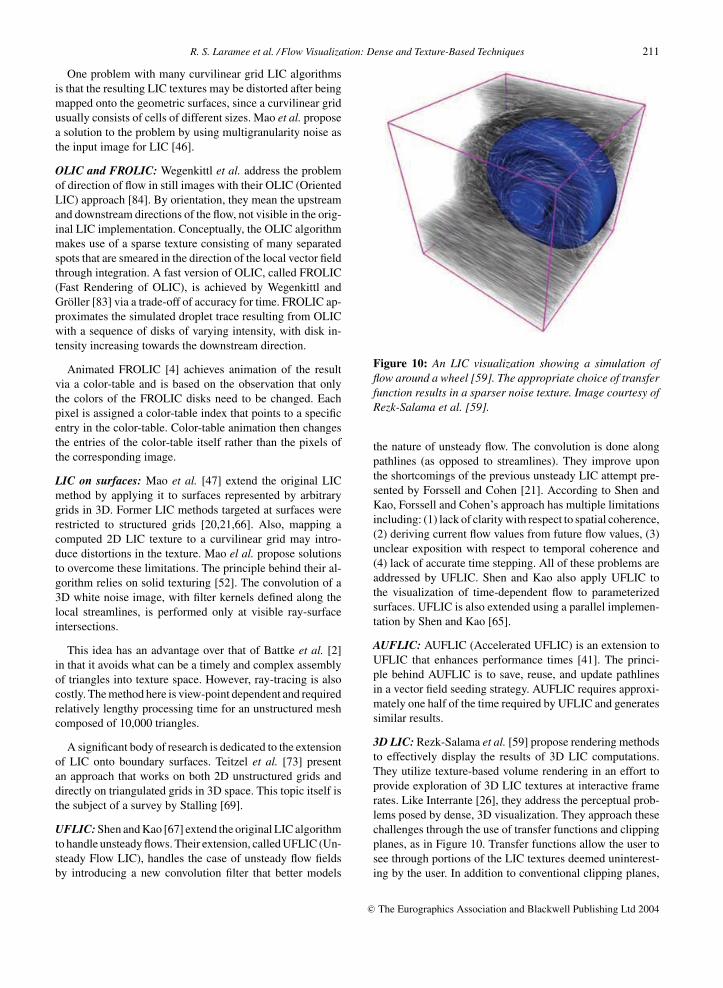
Figure 10: An LIC visualization showing a simulation offlow around a wheel [59]. The appropriate choice of transferfunction results in a sparser noise texture. Image courtesy ofRezk-Salama et al. [59].

the nature of unsteady flow. The convolution is done alongpathlines (as opposed to streamlines). They improve uponthe shortcomings of the previous unsteady LIC attempt pre-sented by Forssell and Cohen [21]. According to Shen andKao, Forssell and Cohen’s approach has multiple limitationsincluding: (1) lack of clarity with respect to spatial coherence,(2) deriving current flow values from future flow values, (3)unclear exposition with respect to temporal coherence and(4) lack of accurate time stepping. All of these problems areaddressed by UFLIC. Shen and Kao also apply UFLIC tothe visualization of time-dependent flow to parameterizedsurfaces. UFLIC is also extended using a parallel implemen-tation by Shen and Kao [65].

AUFLIC: AUFLIC (Accelerated UFLIC) is an extension toUFLIC that enhances performance times [41]. The princi-ple behind AUFLIC is to save, reuse, and update pathlinesin a vector field seeding strategy. AUFLIC requires approxi-mately one half of the time required by UFLIC and generatessimilar results.

3D LIC: Rezk-Salama et al. [59] propose rendering methodsto effectively display the results of 3D LIC computations.They utilize texture-based volume rendering in an effort toprovide exploration of 3D LIC textures at interactive framerates. Like Interrante [26], they address the perceptual prob-lems posed by dense, 3D visualization. They approach thesechallenges through the use of transfer functions and clippingplanes, as in Figure 10. Transfer functions allow the user tosee through portions of the LIC textures deemed uninterest-ing by the user. In addition to conventional clipping planes,



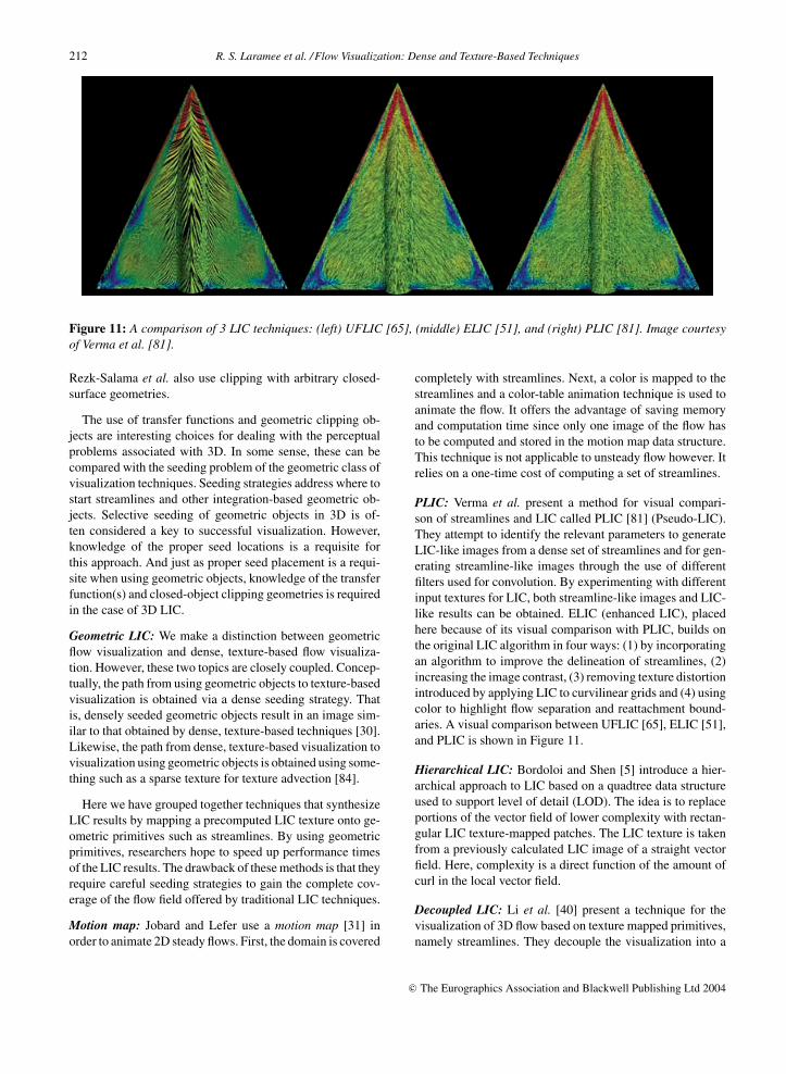
Figure 11: A comparison of 3 LIC techniques: (left) UFLIC [65], (middle) ELIC [51], and (right) PLIC [81]. Image courtesyof Verma et al. [81].

Rezk-Salama et al. also use clipping with arbitrary closed-surface geometries.

The use of transfer functions and geometric clipping ob-jects are interesting choices for dealing with the perceptualproblems associated with 3D. In some sense, these can becompared with the seeding problem of the geometric class ofvisualization techniques. Seeding strategies address where tostart streamlines and other integration-based geometric ob-jects. Selective seeding of geometric objects in 3D is of-ten considered a key to successful visualization. However,knowledge of the proper seed locations is a requisite forthis approach. And just as proper seed placement is a requi-site when using geometric objects, knowledge of the transferfunction(s) and closed-object clipping geometries is requiredin the case of 3D LIC.

Geometric LIC: We make a distinction between geometricflow visualization and dense, texture-based flow visualiza-tion. However, these two topics are closely coupled. Concep-tually, the path from using geometric objects to texture-basedvisualization is obtained via a dense seeding strategy. Thatis, densely seeded geometric objects result in an image sim-ilar to that obtained by dense, texture-based techniques [30].Likewise, the path from dense, texture-based visualization tovisualization using geometric objects is obtained using some-thing such as a sparse texture for texture advection [84].

Here we have grouped together techniques that synthesizeLIC results by mapping a precomputed LIC texture onto ge-ometric primitives such as streamlines. By using geometricprimitives, researchers hope to speed up performance timesof the LIC results. The drawback of these methods is that theyrequire careful seeding strategies to gain the complete cov-erage of the flow field offered by traditional LIC techniques.

Motion map: Jobard and Lefer use a motion map [31] inorder to animate 2D steady flows. First, the domain is covered

completely with streamlines. Next, a color is mapped to thestreamlines and a color-table animation technique is used toanimate the flow. It offers the advantage of saving memoryand computation time since only one image of the flow hasto be computed and stored in the motion map data structure.This technique is not applicable to unsteady flow however. Itrelies on a one-time cost of computing a set of streamlines.

PLIC: Verma et al. present a method for visual compari-son of streamlines and LIC called PLIC [81] (Pseudo-LIC).They attempt to identify the relevant parameters to generateLIC-like images from a dense set of streamlines and for gen-erating streamline-like images through the use of differentfilters used for convolution. By experimenting with differentinput textures for LIC, both streamline-like images and LIC-like results can be obtained. ELIC (enhanced LIC), placedhere because of its visual comparison with PLIC, builds onthe original LIC algorithm in four ways: (1) by incorporatingan algorithm to improve the delineation of streamlines, (2)increasing the image contrast, (3) removing texture distortionintroduced by applying LIC to curvilinear grids and (4) usingcolor to highlight flow separation and reattachment bound-aries. A visual comparison between UFLIC [65], ELIC [51],and PLIC is shown in Figure 11.

Hierarchical LIC: Bordoloi and Shen [5] introduce a hier-archical approach to LIC based on a quadtree data structureused to support level of detail (LOD). The idea is to replaceportions of the vector field of lower complexity with rectan-gular LIC texture-mapped patches. The LIC texture is takenfrom a previously calculated LIC image of a straight vectorfield. Here, complexity is a direct function of the amount ofcurl in the local vector field.

Decoupled LIC: Li et al. [40] present a technique for thevisualization of 3D flow based on texture mapped primitives,namely streamlines. They decouple the visualization into a



Figure 12: The classification of texture advection and GPU-based techniques. The columns indicate the primitive used duringadvection while the rows indicate the advection scheme.

preprocessing type stage that computes the streamlines anda stage which maps various textures to the streamlines com-puted in the first stage. The result is volume rendered at inter-active frame rates. To address the perceptual challenges posedby 3D visualization, depth cues, lighting effects, silhouettes,shading and interactive volume culling are described.

3.3. Texture advection and GPU-based techniques

In this section we describe research based on moving texelsor moving groups of texels, i.e. texture-mapped polygonswhose motion is directed by the vector field. Figure 12 showsan overview of the different techniques and classifies themaccording to two properties: (1) the advection scheme usedand (2) the primitive used during advection. Some of theliterature focuses mainly on the integration scheme used toadvect textures or texels. By the term texel means textureelement. Some methods focus on the mapping to advectedprimitives and some focus on both. Figure 12 also shows thedimensionality of the flow data. In our discussion, we visitthe methods in clockwise order starting at 12 o’clock. Withineach sub-block the methods are listed in chronological order.This is because the mapping of texel properties between twotime steps in the visualization is not 1-to-1 in this case. For amore detailed discussion see Jobard et al. [28,29].

One characteristic common to many of the texture advec-tion techniques in this section [28,29,38,48] is the use ofbackward coordinate integration (or backward advection).None of the methods described here use forward advection(i.e. forward integration) and individual texels as a primi-tive. This is because the combination of forward integrationand texel primitives leaves holes in the visual domain afterthe forward integration computation [29]. Given a position,x0(i , j) = (i , j) of each particle in a 2D flow, backward in-tegration over a time interval h determines its position at aprevious time step [28]:

x−h(i, j) = x0(i, j) +∫ h

τ=0v−τ (x−τ (i, j)) dτ (8)

where h is the integration step, x−τ (i , j) represents interme-diary positions along the pathline passing through x0(i, j),

Figure 13: A screen shot from the image based flow visual-ization algorithm. Image courtesy of Van Wijk [79].

and vτ is the vector field at time τ . We note that the meth-ods in this category are generally implemented in an iterativefashion. That is for each animated frame an integration isperformed over a small time-step h, followed by an updateof visual properties. This is opposed to geometric methods inwhich a longer particle path may be computed over severaltime steps before the results are displayed.

IBFV: Image based flow visualization (IBFV) by Van Wijk[79] is one of the fastest algorithms for dense, 2D, unsteadyvector field representations (Figure 13). It is based on the ad-vection and decay of textures in image space. Each frame ofthe visualization is defined as a blend between the previousimage, warped according to the flow direction, and a num-ber of background images composed of filtered white noisetextures. One reason it is faster than many texture-based flowvisualization methods is because it reduces the number of



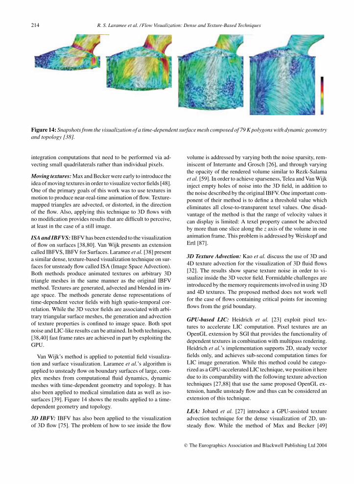
Figure 14: Snapshots from the visualization of a time-dependent surface mesh composed of 79 K polygons with dynamic geometryand topology [38].

integration computations that need to be performed via ad-vecting small quadrilaterals rather than individual pixels.

Moving textures: Max and Becker were early to introduce theidea of moving textures in order to visualize vector fields [48].One of the primary goals of this work was to use textures inmotion to produce near-real-time animation of flow. Texture-mapped triangles are advected, or distorted, in the directionof the flow. Also, applying this technique to 3D flows withno modification provides results that are difficult to perceive,at least in the case of a still image.

ISA and IBFVS: IBFV has been extended to the visualizationof flow on surfaces [38,80]. Van Wijk presents an extensioncalled IBFVS, IBFV for Surfaces. Laramee et al. [38] presenta similar dense, texture-based visualization technique on sur-faces for unsteady flow called ISA (Image Space Advection).Both methods produce animated textures on arbitrary 3Dtriangle meshes in the same manner as the original IBFVmethod. Textures are generated, advected and blended in im-age space. The methods generate dense representations oftime-dependent vector fields with high spatio-temporal cor-relation. While the 3D vector fields are associated with arbi-trary triangular surface meshes, the generation and advectionof texture properties is confined to image space. Both spotnoise and LIC-like results can be attained. In both techniques,[38,40] fast frame rates are achieved in part by exploiting theGPU.

Van Wijk’s method is applied to potential field visualiza-tion and surface visualization. Laramee et al.’s algorithm isapplied to unsteady flow on boundary surfaces of large, com-plex meshes from computational fluid dynamics, dynamicmeshes with time-dependent geometry and topology. It hasalso been applied to medical simulation data as well as iso-surfaces [39]. Figure 14 shows the results applied to a time-dependent geometry and topology.

3D IBFV: IBFV has also been applied to the visualizationof 3D flow [75]. The problem of how to see inside the flow

volume is addressed by varying both the noise sparsity, rem-iniscent of Interrante and Grosch [26], and through varyingthe opacity of the rendered volume similar to Rezk-Salamaet al. [59]. In order to achieve sparseness, Telea and Van Wijkinject empty holes of noise into the 3D field, in addition tothe noise described by the original IBFV. One important com-ponent of their method is to define a threshold value whicheliminates all close-to-transparent texel values. One disad-vantage of the method is that the range of velocity values itcan display is limited: A texel property cannot be advectedby more than one slice along the z axis of the volume in oneanimation frame. This problem is addressed by Weiskopf andErtl [87].

3D Texture Advection: Kao et al. discuss the use of 3D and4D texture advection for the visualization of 3D fluid flows[32]. The results show sparse texture noise in order to vi-sualize inside the 3D vector field. Formidable challenges areintroduced by the memory requirements involved in using 3Dand 4D textures. The proposed method does not work wellfor the case of flows containing critical points for incomingflows from the grid boundary.

GPU-based LIC: Heidrich et al. [23] exploit pixel tex-tures to accelerate LIC computation. Pixel textures are anOpenGL extension by SGI that provides the functionality ofdependent textures in combination with multipass rendering.Heidrich et al.’s implementation supports 2D, steady vectorfields only, and achieves sub-second computation times forLIC image generation. While this method could be catego-rized as a GPU-accelerated LIC technique, we position it heredue to its comparability with the following texture advectiontechniques [27,88] that use the same proposed OpenGL ex-tension, handle unsteady flow and thus can be considered anextension of this technique.

LEA: Jobard et al. [27] introduce a GPU-assisted textureadvection technique for the dense visualization of 2D, un-steady flow. While the method of Max and Becker [49]



Figure 15: Three images taken from an animation of an unsteady vector field created with the Lagrangian-Eulerian advectionalgorithm. [28,29] Image courtesy of Jobard et al.

advects textures based on coarse triangular meshes, Jobardet al. advect textures on a per-pixel basis by means of pixeltextures, which are used in a similar way as by Heidrich et al.[23]. The gray-scale texture from the previous time step isdragged along the flow field by modifying the texture coordi-nates for the dependent texture lookup according to the flowdata. Nearest-neighbor sampling is combined with an updateof fractional texture coordinates to represent subtexel motionand, at the same time, maintain a high contrast. An itera-tive injection of additional noise is used to compensate for apossible loss of contrast over time. Jobard et al. also discussthe treatment of inflow at boundaries, image enhancement bycolor masking and the use of dye advection. Because of thelimited functionality of the graphics hardware that supportspixel textures, the implementation requires many renderingpasses and advects a texture of size 2562 at approximatelytwo frames per second. Moreover, the maximum resolutionof textures is restricted to 2562.

Jobard et al. extend this method to the more flexibleLagrangian-Eulerian Advection (LEA) scheme [28] for thevisualization of unsteady, 2D flow. Here, they rely on a CPUimplementation that leads to better advection quality, higherspeed, and no limitations of the maximum flow size. Particlepaths are integrated as a function of time, referred to as theLagrangian step, while the color distribution of the imagepixels is stored in a texture and updated in place (Eulerianstep). The temporal coherence of the advected noise texturesis transformed into spatial coherence by blending texturesfrom subsequent time steps, i.e. each still frame depicts theinstantaneous structure of the flow, whereas an animated se-quence of frames still reveals the motion of the advected tex-ture. Jobard et al. demonstrate that the combination of noiseand dye advection is useful for an effective visualization andexploration of unsteady flow. Some results from the techniqueare shown in Figure 15. This work is extended by Jobard et al.[29] in order to improve the quality of dye advection.

Weiskopf et al. [86] present a GPU-accelerated versionof the LEA algorithm using per-fragment operations. The

GPU-based texture advection by Weiskopf et al. [88] sup-ports bilinear dependent texture lookups without taking intoaccount the update of fractional coordinates. Therefore, thisapproach is mainly suitable for dye advection at high framerates. Weiskopf et al. also demonstrate how GPU-acceleratedvisualization of unsteady, 3D flows can be implemented withpixel textures.

UFAC: Weiskopf et al. [85] introduce a generic texture-basedframework for visualizing 2D, time-dependent vector fields.They propose unsteady flow advection convolution (UFAC)as an application of the framework for visualizing unsteadyfluid flow. Also, their approach can reproduce other tech-niques such as LEA [29], IBFV [79], UFLIC [65], and DLIC[71]. Weiskopf et al. describe a GPU-accelerated implemen-tation that, among other things, allows the user to trade-offquality for speed.

3.4. Related dense, texture-based methods

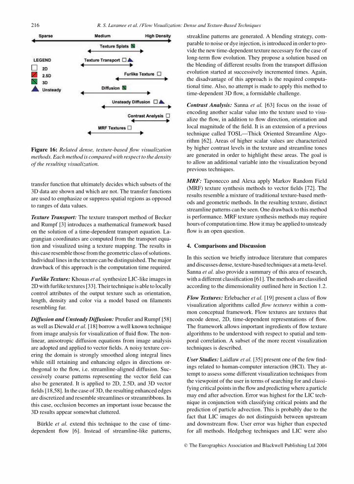
The literature described here is not, in general, as stronglyinterrelated as the literature in the spot noise, LIC, texture ad-vection and GPU-based categories. For this reason we soughtan alternative schema in order to relate the different tech-niques. Figure 16 shows the related methods and classifiesthem based on the density of their results. In this case eachtechnique is given a subjective rating on a sparse-to-densescale. Sparse results look more like the results from flow vi-sualization using geometric objects whereas dense techniquesproduce results resembling spot noise or LIC. These methodsdo not fit cleanly into one of the previous categories; nonethe-less, they are important to the dedicated topic and are brieflyoutlined here. Reading from top to bottom in Figure 16, wevisit the techniques in chronological order.

Texture Splats: As an extension of the technique of splattingfrom volume rendering, Crawfis and Max [9] introduce thenotion of texture splats for flow visualization. Being a vol-ume rendering technique, it is targeted at the depiction of 3Dvector fields. As with Rezk-Salama et al. [59], it is a selective



Figure 16: Related dense, texture-based flow visualizationmethods. Each method is compared with respect to the densityof the resulting visualization.

transfer function that ultimately decides which subsets of the3D data are shown and which are not. The transfer functionsare used to emphasize or suppress spatial regions as opposedto ranges of data values.

Texture Transport: The texture transport method of Beckerand Rumpf [3] introduces a mathematical framework basedon the solution of a time-dependent transport equation. La-grangian coordinates are computed from the transport equa-tion and visualized using a texture mapping. The results inthis case resemble those from the geometric class of solutions.Individual lines in the texture can be distinguished. The majordrawback of this approach is the computation time required.

Furlike Texture: Khouas et al. synthesize LIC-like images in2D with furlike textures [33]. Their technique is able to locallycontrol attributes of the output texture such as orientation,length, density and color via a model based on filamentsresembling fur.

Diffusion and Unsteady Diffusion: Preußer and Rumpf [58]as well as Diewald et al. [18] borrow a well known techniquefrom image analysis for visualization of fluid flow. The non-linear, anisotropic diffusion equations from image analysisare adopted and applied to vector fields. A noisy texture cov-ering the domain is strongly smoothed along integral lineswhile still retaining and enhancing edges in directions or-thogonal to the flow, i.e. streamline-aligned diffusion. Suc-cessively coarse patterns representing the vector field canalso be generated. It is applied to 2D, 2.5D, and 3D vectorfields [18,58]. In the case of 3D, the resulting enhanced edgesare discretized and resemble streamlines or streamribbons. Inthis case, occlusion becomes an important issue because the3D results appear somewhat cluttered.

Burkle et al. extend this technique to the case of time-dependent flow [6]. Instead of streamline-like patterns,

streakline patterns are generated. A blending strategy, com-parable to noise or dye injection, is introduced in order to pro-vide the new time-dependent texture necessary for the case oflong-term flow evolution. They propose a solution based onthe blending of different results from the transport diffusionevolution started at successively incremented times. Again,the disadvantage of this approach is the required computa-tional time. Also, no attempt is made to apply this method totime-dependent 3D flow, a formidable challenge.

Contrast Analysis: Sanna et al. [63] focus on the issue ofencoding another scalar value into the texture used to visu-alize the flow, in addition to flow direction, orientation andlocal magnitude of the field. It is an extension of a previoustechnique called TOSL—Thick Oriented Streamline Algo-rithm [62]. Areas of higher scalar values are characterizedby higher contrast levels in the texture and streamline tonesare generated in order to highlight these areas. The goal isto allow an additional variable into the visualization beyondprevious techniques.

MRF: Taponecco and Alexa apply Markov Random Field(MRF) texture synthesis methods to vector fields [72]. Theresults resemble a mixture of traditional texture-based meth-ods and geometric methods. In the resulting texture, distinctstreamline patterns can be seen. One drawback to this methodis performance. MRF texture synthesis methods may requirehours of computation time. How it may be applied to unsteadyflow is an open question.

4. Comparisons and Discussion

In this section we briefly introduce literature that comparesand discusses dense, texture-based techniques at a meta-level.Sanna et al. also provide a summary of this area of research,with a different classification [61]. The methods are classifiedaccording to the dimensionality outlined here in Section 1.2.

Flow Textures: Erlebacher et al. [19] present a class of flowvisualization algorithms called flow textures within a com-mon conceptual framework. Flow textures are textures thatencode dense, 2D, time-dependent representations of flow.The framework allows important ingredients of flow texturealgorithms to be understood with respect to spatial and tem-poral correlation. A subset of the more recent visualizationtechniques is described.

User Studies: Laidlaw et al. [35] present one of the few find-ings related to human-computer interaction (HCI). They at-tempt to assess some different visualization techniques fromthe viewpoint of the user in terms of searching for and classi-fying critical points in the flow and predicting where a particlemay end after advection. Error was highest for the LIC tech-nique in conjunction with classifying critical points and theprediction of particle advection. This is probably due to thefact that LIC images do not distinguish between upstreamand downstream flow. User error was higher than expectedfor all methods. Hedgehog techniques and LIC were also



associated with high error for locating critical points. Theauthors postulate that this was because in many cases criticalpoints near the borders of the vector field were difficult toidentify.

5. Conclusions and Future Prospects

Texture-based flow visualization algorithms are effective,versatile, and applicable to a wide spectrum of applications. Alarge number of techniques have been developed and refined.In general, which techniques are best depends strongly onthe goal of the visualization, such as for exploration, detailedanalysis, or presentation and on the kind of data involved.Therefore, we believe that a large variety of techniques shouldbe available in order to allow researchers to choose the mostsuitable one.

The problem of dense, 2D, unsteady flow visualization isclose to being solved [79]. And with recent follow-up work[38,80], unsteady flow visualization on surfaces is not farbehind. However, the generalization to 3D flow fields is stillunsolved, especially in the case of unsteady flow. Hardware,arguably, will not be the primary bottleneck to solving thischallenge, but perceptual issues will. Perceiving three spatialand three data dimensions directly is a difficult job for thehuman eye and brain. So far, techniques based on geometricobjects and particle animation generalize better to 3D fields.

The scale of numerical flow simulations, and thus thesize of the resulting datasets, continues to grow rapidly—generally faster than the size of computer memory. For thesereasons more simplification strategies must be conceived,such as spatial selection (slicing, regions of interest), geom-etry simplification and feature extraction.

Slicing in a 3D field reduces the problem to 2D, allowinguse of good 2D techniques, but care must be taken with in-terpretation, as the loss of the third dimension may lead tophysically irrelevant results and wrong interpretation. Takinga single 3D time slice from a 3D time-dependent dataset hassimilar dangers. Other spatial selections such as 3D region-of-interest selection are less risky, but may lead to loss of con-text. Reduction of data dimension, such as reducing vectorquantities to scalars will give more freedom of choice in vi-sualization techniques (such as using volume rendering), butwill not lead to much data reduction. Geometry simplificationtechniques such as polygon mesh decimation, levels-of-detailor multiresolution techniques will be effective in managingvery large datasets and interactive exploration, enabling usersto trade accuracy with response time. Some areas that needadditional work are:

� dense visualization techniques in 3D,� multifield visualization with scalar, vector and tensor

data,� handling and exploring huge time-dependent flow

datasets,

� user studies for evaluation, validation and field testing offlow visualization techniques,

� visualization of inaccuracy and uncertainty [42,60],� more robust feature extraction techniques, especially in

the case of 3D flow.

We also note that much of the research literature presentedhere demonstrates methods operating on structured, uniformresolution grids. However, the grids used in the private, com-mercial industry sector are often adaptive resolution and un-structured, especially in the case of CFD [37,38]. Thus, fur-ther research is necessary in order to integrate many of thethese methods into practical industrial applications.

Acknowledgements

The authors thank all those who have contributed to this re-search including AVL (www.avl.com), the Austrian govern-mental research program called K plus (www.kplus.at) andthe VRVis Research Center (www.VRVis.at). Furthermore,the authors thank all the colleagues from the research commu-nity who permitted to use the images as shown in the paper.CFD simulation data used in Figures 2, 6, 9 and 14 courtesyof AVL.

This project was partly supported by the Netherlands Or-ganization for Scientific Research (NWO) on the NWO-EWComputational Science Project, “Direct Numerical Simu-lation of Oil/Water Mixtures Using Front Capturing Tech-niques”, and by the Landesstiftung Baden-Wurttembergwithin the “Eliteforderprogramm fur Postdoktoranden”.

For supplementary material, including additional,higher resolution images and animations, please visit:http://www.vrvis.at/ar3/pr2/star/

References

1. D. Arrowsmith and C. Place. An Introduction to Dynam-ical Systems. Cambridge University Press, USA, 1990.

2. H. Battke, D. Stalling and H. Hege. Fast Line IntegralConvolution for Arbitrary Surfaces in 3D. In Visual-ization and Mathematics, Springer-Verlag, Heidelberg,pp. 181–195. 1997.

3. J. Becker and M. Rumpf. Visualization of Time-Dependent Velocity Fields by Texture Transport. In Vi-sualization in Scientific Computing ’98, Eurographics,pp. 91–102, 1998.

4. S. Berger and E. Groller. Color-Table Animation of FastOriented Line Intgral Convolution for Vector Field Vi-sualization. In WSCG 2000 Conference Proceedings,pp. 4–11, 2000.



5. U. Bordoloi and H. W. Shen. Hardware AcceleratedInteractive Vector Field Visualization: A level of de-tail approach. In Eurographics 2002 Proceedings, vol-ume 21(3) of Computer Graphics Forum, pp. 605–614,2002.

6. D. Burkle, T. Preußer and M. Rumpf. Transport andAnisotropic Diffusion in Time-Dependent Flow Visu-alization. In Proceedings IEEE Visualization ’01, IEEEComputer Society, pp. 61–67, 2001.

7. B. Cabral and C. Leedom. Highly Parallel Vector Visu-alization Using Line Integral Convolution. In Proceed-ings of the 27th Conference on Parallel Processing forScientific Computing, SIAM Press, USA, pp. 802–807,1995.

8. B. Cabral and L. C. Leedom. Imaging Vector Fields Us-ing Line Integral Convolution. In Poceedings of ACMSIGGRAPH 1993, Annual Conference Series, ACMPress/ACM SIGGRAPH, pp. 263–272, 1993.

9. R. A. Crawfis and N. Max. Texture Splats for 3D Scalarand Vector Field Visualization. In Proceedings IEEE Vi-sualization ’93, IEEE Computer Society, pp. 261–267,Oct. 1993.

10. W. de Leeuw and R. van Liere. Visualization of GlobalFlow Structures Using Multiple Levels of Topology. InData Visualization ’99, Eurographics, Springer-Verlag,pp. 45–52, May 1999.

11. W. de Leeuw and R. van Liere. Multi-Level Topol-ogy for Flow Visualization. Computers and Graphics,24(3):325–331, June 2000.

12. W. de Leeuw and J. van Wijk. Enhanced Spot Noise forVector Field Visualization. In Proceedings IEEE Visual-ization ’95, IEEE Computer Society, pp. 233–239, Oct.1995.

13. W. C. de Leeuw. Divide and Conquer Spot Noise. InProceedings of Supercomputing’97 (CD-ROM), ACMSIGARCH and IEEE, Nov. 1997.

14. W. C. de Leeuw, H. Pagendarm, F. H. Post and B.Waltzer. Visual Simulation of Experimental Oil-FlowVisualization by Spot Noise from Numerical Flow Sim-ulation. In Visualization in Scientific Computing ’95,Springer-Verlag, pp. 135–148, May 1995.

15. W. C. de Leeuw, F. H. Post and R. W. Vaatstra. Visu-alization of Turbulent Flow by Spot Noise. In VirtualEnvironments and Scientific Visualization ’96, Springer-Verlag, pp. 286–295, Apr. 1996.

16. W. C. de Leeuw and R. van Liere. Spotting Structurein Complex Time Dependent Flow. In H. Hagen, G. M.

Nielson and F. H. Post eds Scientific Visualization, IEEE,Dagstuhl Seminar 9724, pp. 9–13, June 1997.

17. W. C. de Leeuw and R. van Liere. Comparing LICand Spot Noise. In Proceedings IEEE Visualization ’98,IEEE Computer Society, pp. 359–366, 1998.

18. U. Diewald, T. Preußer and M. Rumpf. AnisotropicDiffusion in Vector Field Visualization onEuclideanDomains and Surfaces. In IEEE Transactions on Vi-sualization and Computer Graphics, 6(2):139–149,2000.

19. G. Erlebacher, B. Jobard and D. Weiskopf. Flow Tex-tures. In C. R. Johnson and C. D. Hansen (eds), TheVisualization Handbook. Academic Press, Oct. 2003.

20. L. K. Forssell. Visualizing Flow over Curvilinear GridSurfaces Using Line Integral Convolution. In Proceed-ings IEEE Visualization ’94, IEEE Computer Society,pp. 240–247, Oct. 1994.

21. L. K. Forssell and S. D. Cohen. Using Line IntegralConvolution for Flow Visualization: Curvilinear Grids,Variable-Speed Animation, and Unsteady Flows. IEEETransactions on Visualization and Computer Graphics,1(2):133–141, June 1995.

22. H. Hege and D. Stalling. Fast LIC with Piecewise Poly-nomial Filter Kernels. In Mathematical Visualization,Springer Verlag, pp. 295–314, 1998.

23. W. Heidrich, R. Westermann, H.-P. Seidel and T. Ertl.Applications of Pixel Textures in Visualization and Real-istic Image Synthesis. In ACM Symposium on Interactive3D Graphics, pp. 127–134, 1999.

24. L. Hesselink, F. H. Post and J. van Wijk. Research Issuesin Vector and Tensor Field Visualization. IEEE Com-puter Graphics and Applications, 14(2):76–79, Mar.1994.

25. V. Interrante and C. Grosch. Strategies for EffectivelyVisualizing 3D Flow with Volume LIC. In ProceedingsIEEE Visualization ’97, pp. 421–424, 1997.

26. V. Interrante and C. Grosch. Visualizing 3D flow. IEEEComputer Graphics & Applications, 18(4):49–53, 1998.

27. B. Jobard, G. Erlebacher and M. Y. Hussaini. Hardware-Accelerated Texture Advection. In Proceedings IEEEVisualization 2000, IEEE Computer Society, pp. 155–162, 2000.

28. B. Jobard, G. Erlebacher and M. Y. Hussaini.Lagrangian-Eulerian Advection for Unsteady Flow Vi-sualization. In Proceedings IEEE Visualization ’01,IEEE, October 2001.



29. B. Jobard, G. Erlebacher and Y. Hussaini. Lagrangian-Eulerian Advection of Noise and Dye Textures for Un-steady Flow Visualization. IEEE Transactions on Visu-alization and Computer Graphics, 8(3):211–222, 2002.

30. B. Jobard and W. Lefer. Creating Evenly–SpacedStreamlines of Arbitrary Density. In Proceedings ofthe Eurographics Workshop on Visualization in Scien-tific Computing ’97, volume 7, Eurographics, Springer-Verlag, April 28–30, 1997.

31. B. Jobard and W. Lefer. The Motion Map: EfficientComputation of Steady Flow Animations. In Proceed-ings IEEE Visualization ’97, IEEE Computer Society,pp. 323–328, Oct. 19–24, 1997.

32. D. Kao, B. Zhang, K. Kim and A. Pang. 3D Flow Visual-ization Using Texture Advection. In International Con-ference on Computer Graphics and Imaging ’01, August2001.

33. L. Khouas, C. Odet and D. Friboulet. 2D Vec-tor Field Visualization Using Furlike Texture. InJoint Eurographics-IEEE TVCG Symposium on Visu-alization (VisSym ’99), Eurographics, Springer-Verlag,pp. 35–44, May 1999.

34. M. Kiu and D. C. Banks. Multi-frequency Noise for LIC.In Proceedings IEEE Visualization ’96, IEEE, pp. 121–126, Oct. 27–Nov. 1, 1996.

35. D. H. Laidlaw, R. M. Kirby, J. S. Davidson, T. S. Miller,M. da Silva, W. H. Warren and M. Tarr. QuantitativeComparative Evaluation of 2D Vector Field Visualiza-tion Methods. In Proceedings IEEE Visualization 01,IEEE Computer Society, pp. 143–150, October 2001.

36. D. A. Lane. Scientific Visualization of Large-Scale Un-steady Fluid Flows, Scientific Visualization: Overviews,Methodologies, and Techniques. IEEE Computer Sci-ence Press, Los Alamitos, chapter 5, pp. 125–145,1997.

37. R. S. Laramee. FIRST: A Flexible and Interactive Re-sampling Tool for CFD Simulation Data. Computers &Graphics, 27(6):905–916, 2003.

38. R. S. Laramee, B. Jobard and H. Hauser. Image SpaceBased Visualization of Unsteady Flow on Surfaces. InProceedings IEEE Visualization ’03, IEEE ComputerSociety, pp. 131–138, 2003.

39. R. S. Laramee, J. Schneider and H. Hauser. Texture-Based Flow Visualization on Isosurfaces from Com-putational Fluid Dynamics. In Joint Eurographics—IEEE TVCG Symposium on Visualization (VisSym ’04),Konstanz, Germany, May 19–21, 2004, forthcoming.

40. G. S. Li, U. Bordoloi and H. W. Shen. Chameleon:An Interactive Texture-based Framework for VisualizingThree-dimensional Vector Fields. In Proceedings IEEEVisualization ’03, IEEE Computer Society, pp. 241–248,2003.

41. Z. P. Liu and R. J. Moorhead, II. AUFLIC: An Acceler-ated Algorithm for Unsteady Flow Line Integral Convo-lution. In Proceedings of the Joint Eurographics—IEEETCVG Symposium on Visualizatation (VisSym ’02),pp. 43–52, 2002.

42. S. K. Lodha, A. Pang, R. E. Sheehan and C. M. Witten-brink. UFLOW: Visualizing Uncertainty in Fluid Flow.In Proceedings IEEE Visualization ’96, pp. 249–254,Oct. 27–Nov. 1, 1996.

43. H. Loffelmann, T. Kucera and E. Groller. VisualizingPoincare Maps Together with the Underlying Flow. InMathematical Visualization, Springer Verlag, pp. 315–328, 1998.

44. H. Loffelmann, L. Mroz, E. Groller and W. Purgathofer.Stream Arrows: Enhancing the Use of Streamsurfacesfor the Visualization of Dynamical Systems. The VisualComputer, 13:359–369, 1997.

45. H. Loffelmann, Z. Szalavari and E. Groller. Local Analy-sis of Dynamical Systems—Concepts and Interpretation.In WSCG 1996 Conference Proceedings, pp. 170–180,Feb. 1996.

46. X. Mao, L. Hong, A. Kaufman, N. Fujita and M.Kikukawa. Multi-Granularity Noise for Curvilinear GridLIC. In Graphics Interface, pp. 193–200, June 1998.

47. X. Mao, M. Kikukawa, N. Fujita and A. Imamiya. LineIntegral Convolution for 3D Surfaces. In Visualizationin Scientific Computing ’97. Proceedings of the Euro-graphics Workshop, pp. 57–70. Eurographics, 1997.

48. N. Max and B. Becker. Flow Visualization Using Mov-ing Textures. In Proceedings of the ICASW/LaRC Sym-posium on Visualizing Time-Varying Data, pp. 77–87,Sept. 1995.

49. N. Max, B. Becker and R. Crawfis. Flow Volumes forInteractive Vector Field Visualization. In ProceedingsIEEE Visualization ’93, IEEE Computer Society, pp. 19–24, Oct. 1993.

50. N. Max, R. Crawfis and D. Williams. Visualizing WindVelocities by Advecting Cloud Textures. In Proceed-ings IEEEVisualization ’92, IEEE Computer Society,1992.

51. A. Okada and D. L. Kao. Enhanced Line Integral Con-volution with Flow Feature Detection. In SPIE Vol. 3017



Visual Data Exploration and Analysis IV , pp. 206–217,Feb. 1997.

52. D. R. Peachey. Solid Texturing of Complex Surfaces.Computer Graphics (Proceedings of ACM SIGGRAPH85), 19(3):279–286, 1985.

53. F. H. Post and T. van Walsum. Fluid flow visualization.In Focus on Scientific Visualization, Springer, pp. 1–40,1993.

54. F. H. Post and J. van Wijk. Visual Representation ofVector Fields: Recent Developments and Research Di-rections. In L. Rosenblum et al. (eds), Scientific Visual-ization: Advances and Challenges. Springer, chapter 23,pp. 367–390, 1994.

55. F. H. Post, B. Vrolijk, H. Hauser, R. S. Laramee andH. Doleisch. Feature Extraction and Visualization ofFlow Fields. In Eurographics 2002 State-of-the-Art Re-ports, The Eurographics Association, pp. 69–100, 2–6,September 2002.

56. F. H. Post, B. Vrolijk, H. Hauser, R. S. Laramee andH. Doleisch. The State of the Art in Flow Visualization:Feature Extraction and Tracking. Computer GraphicsForum, 22(4):775–792, Dec. 2003.

57. W. H. Press, S. A. Teukolsky, W. T. Vettering and B. P.Flannery. Numerical Recipes in C++: The Art of Scien-tific Computing. 2 edition, Cambridge University Press,Cambridge, 2002.

58. T. Preußer and M. Rumpf. Anisotropic Nonlinear Diffu-sion in Flow Visualization. In Proceedings IEEE Visual-ization ’99, IEEE Computer Society, pp. 325–332, Oct.1999.

59. C. Rezk-Salama, P. Hastreiter, C. Teitzel and T. Ertl. In-teractive exploration of volume line integral convolutionbased on 3D-texture mapping. In Proceedings IEEE Vi-sualization ’99, IEEE Computer Society, pp. 233–240,1999.

60. P. J. Rhodes, R. S. Laramee, R. D. Bergeron and T. M.Sparr. Uncertainty Visualization Methods in IsosurfaceRendering. In M. Chover, H. Hagen and D. Tost (eds),Eurographics 2003, Short Papers, The Eurographics As-sociation, pp. 83–88, September 1–5, 2003.

61. A. Sanna, B. Montrucchio and P. Montuschi. A survey onvisualization of vector fields by texture-based methods.Recent Research Developments in Pattern Recognition,1(1):13–27, 2000.

62. A. Sanna, B. Montrucchio, P. Montuschi and A. Spar-avigna. Visualizing Vector Fields: The Thick Oriented

Stream-Line Algorithm (TOSL). Computers and Graph-ics, 25(5):847–855, Oct. 2001.

63. A. Sanna, C. Zunino, B. Montucchio and P. Mon-tuschi. Adding a Scalar Value to Texture-Based Vec-tor Field Representations by local contrast analysis. InProceedings of the Joint Eurographics—IEEE TCVGSymposium on Visualizatation (VisSym ’02), pp. 35–41,2002.

64. G. Scheuermann, H. Burbach and H. Hagen. Visualiz-ing Planar Vector Fields with Normal Component UsingLine Integral Convolution. In Proceedings IEEE Visual-ization ’99, IEEE Computer Society, pp. 255–262, 1999.

65. H. Shen and D. L. Kao. A New Line Integral Con-volution Algorithm for Visualizing Time-Varying FlowFields. IEEE Transactions on Visualization and Com-puter Graphics, 4(2), Apr.–June, pp. 98–108, 1998.

66. H. W. Shen, C. R. Johnson and K. L. Ma. VisualizingVector Fields Using Line Integral Convolution and DyeAdvection. In 1996 Volume Visualization Symposium,IEEE, pp. 63–70, Oct. 1996.

67. H. W. Shen and D. L. Kao. UFLIC: A Line IntegralConvolution Algorithm for Visualizing Unsteady Flows.In Proceedings IEEE Visualization ’97, IEEE ComputerSociety, pp. 317–323, 1997.

68. D. Silver, F. Post, and I. Sadarjoen. Flow Visualization,volume 7 of Wiley Encyclopedia of Electrical and Elec-tronics Engineering, John Wiley & Sons, New York,pp. 640–652, 1999.

69. D. Stalling. LIC on Surfaces. In Texture Synthesis withLine Integral Convolution, ACM SIGGRAPH 97, Inter-national Conference on Computer Graphics and Interac-tive Techniques, pp. 51–64, 1997.

70. D. Stalling and H. Hege. Fast and Resolution Indepen-dent Line Integral Convolution. In Proceedings of ACMSIGGRAPH 95, Annual Conference Series, ACM SIG-GRAPH, ACM Press/ACM SIGGRAPH, pp. 249–256,1995.

71. A. Sundquist. Dynamic Line Iintegral Convolution forVisualizing Streamline Evolution. IEEE Transactionson Visualization and Computer Graphics, 9(3):273–282,2003.

72. F. Taponecco and M. Alexa. Vector Field Visualizationusing Markov Random Field Texture Synthesis. In Pro-ceedings of the Joint Eurographics–IEEE TCVG Sympo-sium on Visualizatation (VisSym ’03), Springer-Verlag,pp. 195–202, May 2003.



73. C. Teitzel, R. Grosso and T. Ertl. Line Integral Convo-lution on Triangulated Surfaces. In WSCG 1997 Confer-ence Proceedings, pp. 572–581, 1997.

74. A. Telea and J. van Wijk. Simplified Representation ofVector Fields. In Proceedings IEEE Visualization ’99,IEEE Computer Society, pp. 35–42, 1999.

75. A. Telea and J. J. van Wijk. 3D IBFV: Hardware-Accelerated 3D Flow Visualization. In ProceedingsIEEE Visualization ’03, IEEE Computer Society,pp. 233–240, 2003.

76. T. Urness, V. Interrante, I. Marusic, E. Longmire, andB. Ganapathisubramani. Effectively Visualizing Multi-Valued Flow Data using Color and Texture. In Proceed-ings IEEE Visualization ’03, IEEE Computer Society,pp. 115–122, 2003.

77. M. van Dyke. An Album of Fluid Motion. The ParabolicPress, 1982.

78. J. J. van Wijk. Spot noise-Texture Synthesis for Data Vi-sualization. InT. W. Sederberg (ed), Computer Graphics(Proceedings of ACM SIGGRAPH 91), ACM, volume25, pp. 309–318, 1991.

79. J. J. van Wijk. Image Based Flow Visualization. ACMTransactions on Graphics, 21(3):745–754, 2002.

80. J. J. van Wijk. Image Based Flow Visualization forCurved Surfaces. In Proceedings IEEE Visualization ’03,IEEE Computer Society, pp. 123–130, 2003.

81. V. Verma, D. Kao and A. Pang. PLIC: Bridging theGap Between Streamlines and LIC. In ProceedingsIEEE Visualization ’99, N.Y., pp. 341–348, Oct. 25–29,1999.

82. H. K. Versteeg and W. Malalasekera. Addison-Wesley,February 1996.

83. R. Wegenkittl and E. Groller. Fast Oriented Line Inte-gral Convolution for Vector Field Visualization via theInternet. In Proceedings IEEE Visualization ’97, IEEEComputer Society, pp. 309–316, Oct. 19–24, 1997.

84. R. Wegenkittl, E. Groller and W. Purgathofer. Animat-ing Flow Fields: Rendering of Oriented Line IntegralConvolution. In Computer Animation ’97 Proceedings,IEEE Computer Society, pp. 15–21, June 1997.

85. D. Weiskopf, G. Erlebacher and T. Ertl. A Texture-Based Framework for Spacetime-Coherent Visualizationof Time-Dependent Vector Fields. In Proceedings IEEEVisualization ’03, IEEE Computer Society, pp. 107–114,2003.

86. D. Weiskopf, G. Erlebacher, M. Hopf and T.Ertl. Hardware-Accelerated Lagrangian-Eulerian Tex-ture Advection for 2D Flow Visualizations. In Proceed-ings of the Vision Modeling and Visualization Confer-ence 2002 (VMV-01), pp. 439–446, Nov. 21–23, 2002.

87. D. Weiskopf and T. Ertl. GPU-Based 3D Texture Ad-vection for the Visualization of Unsteady Flow Fields.In WSCG 2004 Conference Proceedings, Short Papers,pp. 259–266, February 2004.

88. D. Weiskopf, M. Hopf and T. Ertl. Hardware-Accelerated Visualization of Time-Varying 2D and 3DVector Fields by Texture Advection via ProgrammablePer-Pixel Operations. In Proceedings of the Vision Mod-eling and Visualization Conference 2001 (VMV 01),pp. 439–446, Nov. 21–23, 2001.

89. R. Yagel, D. M. Reed, A. Law, P. Shih and N. Shareef.Hardware Assisted Volume Rendering of UnstructuredGrids by Incremental Slicing. In Proceedings 1996 Sym-posium on Volume Visualization, pp. 55–62, Sept. 1996.

90. M. Zockler, D. Stalling and H.-C. Hege. Parallel LineIntegral Convolution. Parallel Computing, 23(7):975–989, 1997.


The State of the Art in Flow Visualization: Dense and Texture-Based ...

Documents

Transcript of The State of the Art in Flow Visualization: Dense and Texture-Based ...