The standard deviation of luminance as a metric for...

Perception, 1990, volume 19, pages 79-101

The standard deviation of luminance as a metric for contrast in random-dot images

Bernard MouldenIT, Fred Kingdom, Linda F Gatley Department of Psychology, University of Reading, White knights, Reading RG6 2AL, Berks, UK Received 7 March 1989, in revised form 31 October 1989

Abstract. Michelson's contrast, C, is an excellent metric for contrast in images with periodic luminance profiles, such as gratings, but is not suitable for images consisting of isolated stimulus elements, eg single bars; other metrics have been devised for such stimuli. But what metric should be used for random-dot images such as are commonly used in stereograms and kinematograms?

Previously the standard deviation (SD) of the luminances (equivalent to the root mean square, RMS, of the amplitudes) has been taken as a measure of contrast, but on little more than intuitive grounds. The validity of this speculative usage is tested. Experiments are described in which a wide range of random-dot images of various compositions was used and the adapting power of these images measured. This was taken as an index of their visual effectiveness. The contrast and contrast-reducing effects of the stimuli were expressed in terms of six candidate metrics, including SD, to discover which would give the most lawful description of the experimental data.

The usefulness and generality of the SD measure were confirmed. The effects of mean luminance were also measured and a general expression that would take them into account was derived. Finally, on the basis of computational modelling in which spatial filters with properties approximating those of retinal ganglion cells were used, a possible theoretical account for the success of the SD metric is offered.

1 Introduction Random-dot images are widely used as stimuli in vision research (eg stereograms, kinematograms, masking noise), and as with all stimuli it is essential to have some metric by which their visual effectiveness may be described. There is, however, no general agreement on, and no sound theoretical basis for, a metric of contrast for random-element stimuli.

1.1 Measures of contrast The most commonly used measure of contrast in visual stimuli is the Michelson contrast expression,

J + / -'-'max ' x-'min

where Lmax and Lmin are respectively the maximum and minimum luminances in the image. This measure was implicitly used by Rayleigh (1889) but first explicitly introduced to the study of physical optics by Michelson (1927) when he used expression (1) C to describe the visibility of interference fringes. The measure came into widespread use after the introduction of Fourier techniques to the study of physical optics. Its use in physiological optics and psychophysics was accelerated by the work of Campbell and Green (1965) and Campbell and Robson (1968) when they demonstrated the explanatory power of Fourier theory in those fields of enquiry. The application of Fourier concepts in each case required a measure of modulation amplitude that is independent of DC level (mean luminance in this case).

If Author to whom all correspondence and requests for reprints should be addressed.

80 B Moulden, F Kingdom, L F Gatley

Michelson's C has been generally accepted as being suitable for simple periodic stimuli, such as sinusoidal or square-wave gratings. In such gratings there are equal proportions of Lmax and Lmin, and the mean of (Lmax + Lmin) is equal to the overall mean luminance of the pattern since every luminance value in the display is evenly distributed throughout the image. The denominator in the expression thus represents (twice) the mean luminance of the display.

Moreover, the numerator represents (twice) the incremental (or decremented) amplitude, AL, of the peak (or trough) above (or below) the mean level, L; the expression is therefore mathematically identical to the expression C = AL/L, and thus has formal similarities to the general Weber fraction AL/L. It is this correspondence between the physical measure C and the physiological response that the Weber fraction approximately describes which makes C such a useful measure of the physical contrast of visual stimuli.

Michelson's C is not suitable, however, for isolated stimulus elements such as a bar on a uniform background, where a commonly used measure of contrast is the Weber fraction:

A = L m a x ~ L m i n . (2)

Here, Lmax and Lmin are respectively the larger and smaller of the bar and background luminances and Lb is the background luminance. The use of the different denominator in this expression compared with the Michelson expression acknowledges the preponderance in this type of stimulus of whichever of Lmax and Lmin is also Lb . Because of the different spatial extents of the two luminances the mean luminance of the display as a whole is not equal to the mean of Lmax and Lmin, but is biased in the direction of Lb . Whittle (1986), for this and other reasons (by the use of Lmin rather than Lb as the denominator his data were linearised for a wide range of increment, decrement, and background contrasts), proposed a similar measure,

= } ' (3)

This takes as the denominator either the luminance of the stimulus or that of the background, whichever is the smaller.

The crucial common feature of simple expressions for contrast such as (2) and (3) (where we have denoted contrast by A and W respectively) is that they contain only the values of Lmax and Lmin. They are therefore suitable just for cases in which the variable of interest is the contrast between two intensities. Michelson's C is appropriate for stimuli containing many intensities, but only if the stimuli are periodic and symmetrical so that the mean of Lmax and Lmin is a good approximation of the overall mean luminance of the pattern.

To sum up, Michelson's C is suitable only for periodic stimuli whereas the measures A and W are suitable only for stimuli which consist essentially of just two grey levels.

When more complex images consisting of multiple and unequally distributed luminances are considered, neither of these classes of expression is suitable as a measure of contrast, because neither can take into account the luminance distribution (see eg Moulden and Kingdom 1987). For instance, the value of Michelson's C for a given pair of values, Lmax and Lmin, will remain constant despite the introduction of any number of intermediate luminances: a square-wave grating and a sine-wave grating with the same amplitude and mean luminance have the same Michelson contrast. Moreover, in the case of periodic stimuli with unequal mark-space ratios the mean of Lmax

(d)

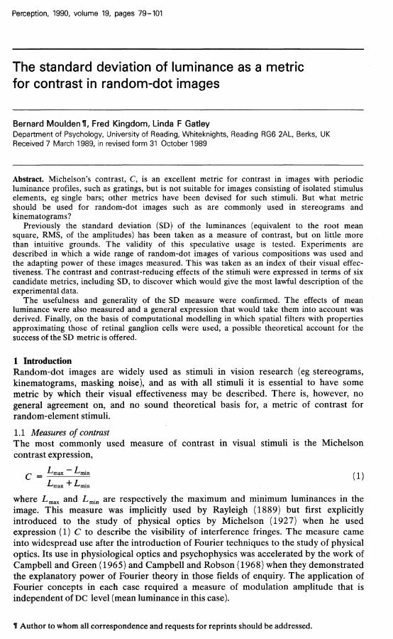
Figure 1. Examples of the kinds of stimuli used, illustrating the spatial configuration and various grey-level distributions, (a) Six grey levels, equal distribution, (b) Four grey levels, inverse binomial distribution, (c) Fourteen grey levels, binomial distribution, (d) Two grey levels, equal distribution. All have the same mean luminance and the same maximum and minimum luminances (Lmax and Lmin respectively); but note the different subjective impression of contrast in each.

82 B Mouiden, F Kingdom, L F Gatley

and Lmin will not be the same as the overall mean luminance, which will thus be misrepresented in the Michelson expression.

In the case of A and W, variations in the relative spatial extents of the different luminances in a display will leave its contrast unchanged according to these metrics. The values of A and W will each be the same irrespective of the width of a bar, for example.

The significance of this point may be illustrated by considering the nonperiodic two-dimensional stimuli shown in figure 1, and the histograms of grey-level probabilities for these and other stimuli shown in figures 2 and 3. The stimuli are composed of random arrangements of pixels which have two (figures Id and 2a-2f) or more (figures l a - lc and 3a-3c) different luminances or 'grey levels'. The various grey levels are distributed among the elements either equally (figures la and 3a), or such that intermediate grey

.a a

o a o

(b)

0 32 62 Luminance/cd m~2

0 32 62

/ J \ /e\ Luminance/ca m " m

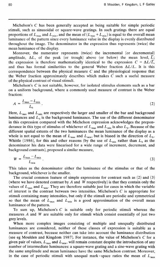
Figure 2. Histograms representing the luminance distribution of the two-grey-level (2GL) stimuli.

0.4 r

0.2

13 'a *o 0

o 0.4 OH O

0.2

(b) 1 2 3 4 5 Grey-level number

32 Luminance/cd m~2

62

2 3 4 5 Grey-level number

0 62 32 Luminance/cd m"2

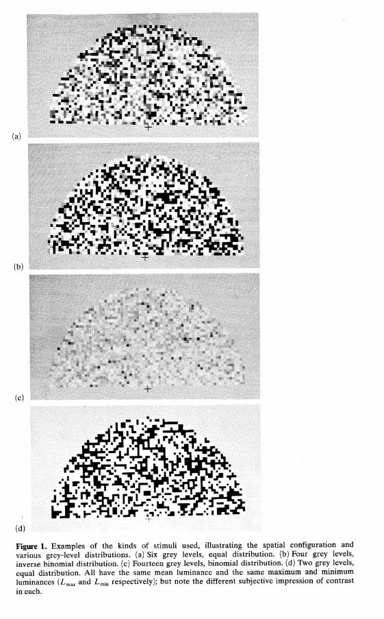
Figure 3. Histograms representing the luminances and their probability of occurrence in multi-grey-level (multiGL) stimuli. In this example all stimuli have six grey levels. Distributions are (a) equal, (b) binomial, and (c) inverse binomial.

Contrast in random-dot images 83

levels occur more frequently than do the extreme ones (figures lc and 3b) or vice versa (figures lb and 3c). Crucially, Lmax and Lmin are the same for all these last four images: the luminances of the light and dark elements in the image with two grey levels (figure Id), for example, are equal to those of the lightest and darkest grey levels respectively in the displays with many grey levels. Consequently the contrasts of all four images are identical when calculated according to definitions (1), (2), and (3). This clearly does not correspond with the subjective impression of contrast in these images.

Whenever values have been given for the visual effectiveness of random-dot images or one-dimensional noise these have generally been in terms of the root mean square (RMS) of the luminance amplitudes of the component elements of the image (Burr 1985; Stanley 1987; Stromeyer and Julesz 1972; Swensson and Judy 1981) or noise spectral density (Burgess et al 1981; Nagaraja 1964), which is the RMS per unit area of visual angle (though see Hamerly et al 1977; Mayhew and Frisby 1978; Quick et al 1976 for an alternative approach). The RMS is simply the standard deviation (SD) of luminance. We have used the standard deviation to model successfully the ability of human observers to detect line signals in visual noise (Kingdom and Moulden 1986; Moulden and Kingdom 1987, 1988). Like others, however, we adopted this measure on little more than intuitive grounds, and our confidence in its appropriateness was based solely upon the empirical fact that it led to a reasonable and lawful description of our data.

1.2 Aims and strategy We therefore wished first to test more directly the assumption that the SD is a suitable measure of the visual effectiveness of random-dot stimuli; second to investigate whether any of a set of other plausible metrics would do as well as or better than the SD; third to discover the generality of the SD metric by using a wide range of different random luminance distributions; fourth to consider how the effect of mean luminance should be taken into account (since the effective contrast of a stimulus with a given SD at a high mean luminance must surely be less than a stimulus with the same SD but a lower mean luminance); and finally to try to understand from a theoretical point of view why SD might be an appropriate measure of visual effectiveness in random-dot images.

To meet these five aims, we first selected as our direct measure of visual effectiveness the adaptive effect of various random-dot images, where the adaptive effect was measured in terms of the degree to which each reduced the apparent contrast of a standard test image. Second, we derived a set of six candidate metrics, including SD, which we judged to be plausible candidates as descriptors of contrast, and calculated our results in terms of all six for comparison purposes. Third, we generated a set of random-dot images which differed in the number of grey levels they contained, their luminance range, and the distribution of grey levels, in order to test the generality of the metrics. Fourth, we measured the effect of mean luminance and derived an expression to take its effect into account. Finally, on the basis of some computational modelling with visual filters with properties approximating those of retinal ganglion cells, we describe a possible theoretical basis for the reason why the SD metric should be as successful as it proved to be in describing the visual effectiveness of random-dot stimuli.

It is well known that exposure to a grating of suprathreshold contrast reduces both contrast sensitivity at threshold (Blakemore and Campbell 1969; Tolhurst 1972) and apparent contrast above threshold (Blakemore et al 1971, 1973; Georgeson 1985) for gratings of a similar spatial frequency and orientation. Increasing the suprathreshold contrast of the adapting pattern increases the magnitude of the aftereffect. Similarly, and as expected, we found in pilot studies that the apparent contrast of suprathreshold random-element stimuli was considerably depressed after adaptation to a high-contrast random-element display. In the formal experiments described below, a


suprathreshold-contrast-matching task was used to measure the adapting effects of stimuli with different numbers and distributions of grey levels on the perceived contrast of a two-grey-level test stimulus of fixed physical contrast. A reduction in the contrast required to make a comparison stimulus (presented to an unadapted part of the retina) appear equal in contrast to a test stimulus (presented to an adapted region) reflects the degree to which the adapting stimulus reduces the apparent contrast of the test stimulus. Stimuli which are differently composed but which have the same contrast according to a particular candidate metric would be expected, if that metric is an appropriate one, to have similar adapting effects. We shall therefore judge any contrast metric to be an appropriate measure if the adaptive effect of a range of stimuli is accounted for by their adapting contrast when both are calculated according to that metric.

2 General method 2.1 Subjects Two of the authors acted as subjects: LG (experiments 1 and 2) and FK (experiments 2 and 3). Both have normal uncorrected vision.

2.2 Apparatus Stimuli were generated by means of a Supervisor 214 (Gresham Lion PPL) graphics/ image system interfaced to a PDP 11/40 host computer. They were displayed on a Digivision TV monitor with a resolution of 512 pixels x 512 pixels, on a screen area 230 mm x 230 mm in size. The luminances of the 256 grey levels available in the system were measured with a UDT (United Detector Technology) microphotometer (model 81) focused onto the phosphor of the monitor when it displayed a large homogeneous patch of pixels. The maximum luminance obtainable was 62 cd m~2 and the maximum number of intensities that could be displayed at any one time was sixteen. A suitable set of intensities was selected on the basis of this calibration.

Each pixel was approximately circular with, at the viewing distance of 120 cm, a diameter of 1.27 min visual angle. By blocking together sixteen pixels (all of the same luminance) larger pixels were formed, of square aspect ratio and side length 5.08 min. The term 'pixel' will be used from now on to refer to these larger pixels.

We confirmed that there were no important 'context-dependent' variations in displayed luminance. Because of a video process known as 'black-level clamping' the luminance on a display seen in response to a fixed voltage applied to the grid to display a pixel can vary as a function of the voltages applied at other points in the raster sweep. In other words, a pixel plotted with a particular intended value on a perfectly black screen may have a different output luminance from that which is generated when it is plotted with the background intensity set to maximum. If this were to happen to any marked degree, then the actual luminance of any pixel in response to a constant signal from the image system would vary as a function of the intensity of other pixels in the display. This would make any assertions about luminance distributions in different displays highly suspect if not useless. No such effects were measurable on our display; we are confident that had any such effects exceeded about 0.5 cd m~2 we would have detected them. Full details of the investigations of potential luminance artifacts with the monitor used here are described in Moulden and Kingdom (1989).

2.3 Stimulus description In describing the display luminance parameters we shall use the following notation: G the number of grey levels in the stimulus. Lt the luminance of the ith grey level; the maximum value of i ranged from 2 to 14

according to condition. Pi the probability of occurrence of the ith grey level.


L the mean luminance of the stimulus, defined as the space-average luminance and calculated numerically by the formula:

G

R the luminance range, defined as the difference between the luminances of the lightest and darkest grey levels in the stimulus (ie Lmax - Lmin).

2.4 Stimuli In order to isolate the effects of contrast adaptation from those of light adaptation, the mean luminance for each stimulus was always equal to the luminance of the homogeneous grey surround on which it appeared. This value was fixed for all displays at 32 cd m 2 . The adaptive state of the subject was therefore held constant throughout. Whereas G in the adapting stimulus could range from 2 to 14 in steps of 2, the test and match stimuli always had G equal to 2. The luminance values of the grey levels for the various stimuli were determined as follows.

2.4.1 Adapting stimuli. For all stimuli with G equal to 2, the probability of occurrence of each grey level was always 0.5 (see below). Thus, because mean luminance was held constant, the luminance values of the two grey levels were determined by the luminance range R. For the test stimulus and two-grey-level (2GL) adapting stimuli R could have a value between 10 and 60 cd m~2 in steps of 10 cd m~2, with Lmax and Lmin always symmetrical about the mean luminance of 32 cd m"2. Figure 2 shows the resulting grey-level histograms. For the match stimulus, R was controlled by the observer.

For all stimuli with G greater than 2 (ie multiGL stimuli), the luminances of the grey levels were selected so as to be spaced at equal linear intervals and, unless otherwise stated, so that R was 60 cd m~2. Luminances were drawn via a look-up table from the palette of 256 available. The palette member nearest to the required value was used in the display.

For each stimulus the grey-level probabilities had one of three possible distributions: (i) Equal distribution of grey levels (E): Each pixel was randomly allocated one of the grey levels / with a probability pt of 1/G. The resulting histogram of grey-level distribution is flat, as in the example shown in figure 3 a. (ii) Binomial distribution of grey levels (B): Each pixel was randomly allocated one of the grey levels i with the probability pt determined by the binomial rule, whereby

N\ p= Ph(l-P)N~h (4) Pl h\(N-h)\ [ ] ' [ )

where N = G—l and h = / - 1. Stimuli were generated with the parameter P in equation (4) set to 0.5 so that the underlying shape of the distribution of grey-level probabilities was symmetrical. Figure 3b shows the resulting grey-level histogram for a stimulus with G equal to 6, for example. (iii) Inverse binomial distribution of grey levels (I): The shape of this distribution of luminances for any given value of G was the inverse of that for the corresponding binomial distribution. The stimulus was generated with the grey-level probabilities for the binomial case effectively redistributed in accordance with the following rule. The probabilities of occurrence for the two grey levels at the extremes of the grey-level scale were interchanged with those for the two grey levels located centrally on the scale; the probabilities for each of the grey levels adjacent to the two extreme levels were interchanged with those for the two grey levels on either side of the central pair, and so on. Such a distribution is illustrated in figure 3c.

The adapting stimuli were drawn from the twenty-four possible combinations of G values, distribution types, and R values, according to the requirements of each


experiment as described below. When individual multiGL stimuli are referred to, the value of G will be given, with a letter symbol (E, B, or J) representing the distribution type (eg 12E indicates a stimulus consisting of twelve equally distributed grey levels).

2.4.2 Metrics for contrast. The luminance characteristics of the 2GL stimuli (equal grey-level distribution and fixed mean luminance L) were such that the assessment of their relative contrasts was straightforward no matter how contrast was measured: the bigger R is, the higher the contrast. Values of the Michelson contrast for the 2GL adapting and test stimuli, which had values of R between 10 and 60 cd m~2, were 0.16, 0.31, 0.47, 0.62, 0.78, and 0.94.

The luminance characteristics of multiGL stimuli (symmetrical grey-level distributions, fixed L, R = 6 0 cd m"2) were such that the grey scale was constrained to begin and end at fixed luminance values (ie Lmax and Lmin were constant values, see figures 3a-3c). Therefore, and by design, Michelson's C does not distinguish between the different multiGL stimuli: the value of C was constant at 0.94.

Six possible methods for measuring the contrast of the random-element stimuli were assessed. Threse metrics and their definitions were: (i) SD, the standard deviation of the untransformed luminances:

I Pi(L-Lf. (5) i

(ii) SDLG, the standard deviation of the logarithm of luminance: G

£ AflogL.-I^r), (6) '" G

where log L = £ P/log L t. i

(iii) SAM, the space-average Michelson contrast: G G \T •- T -\

Zliw/frf1- (7) (iv) SALGM, the space-average logarithm of the Michelson contrast:

G G ' \L,-L,\

\ L> + Li IlAPylogRVr1 • (8)

(v) SAW, the space-average Whittle contrast: G G \L,-L,\ I E ftp; • ' ' v (9)

, / min(L,,Ly)

(vi) SALGW, the space-average logarithm of the Whittle contrast: G c < \L,-L. z j \mm{LhLj) J

These candidate metrics were chosen bearing in mind those findings which seem to suggest some nonlinear transform (commonly a logarithmic transform) of stimulus intensity at an early stage in visual processing (see eg Legge and Kersten 1983; Morgan et al 1984) and also models which assume a linear input stage at a particular operating level (see eg Kingdom and Moulden 1986).

Each candidate metric has the advantage over conventional contrast measures, such as the Michelson contrast, of taking into account the relative amounts of all the different luminances in the stimulus. Each of the 'space-average' metrics (SAM, SALGW, etc) effectively computes the average of all interpixel edge contrasts.


Moreover, each candidate metric appeared, on the basis of informal observation, to reflect at least approximately the subjective impression of contrast in the stimuli, so that all were plausible candidates.

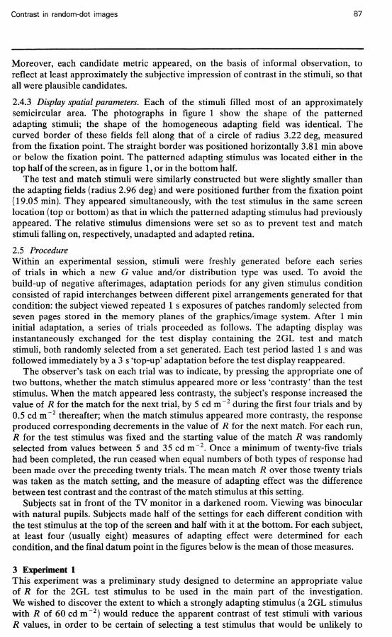
2.4.3 Display spatial parameters. Each of the stimuli filled most of an approximately semicircular area. The photographs in figure 1 show the shape of the patterned adapting stimuli; the shape of the homogeneous adapting field was identical. The curved border of these fields fell along that of a circle of radius 3.22 deg, measured from the fixation point. The straight border was positioned horizontally 3.81 min above or below the fixation point. The patterned adapting stimulus was located either in the top half of the screen, as in figure 1, or in the bottom half.

The test and match stimuli were similarly constructed but were slightly smaller than the adapting fields (radius 2.96 deg) and were positioned further from the fixation point (19.05 min). They appeared simultaneously, with the test stimulus in the same screen location (top or bottom) as that in which the patterned adapting stimulus had previously appeared. The relative stimulus dimensions were set so as to prevent test and match stimuli falling on, respectively, unadapted and adapted retina.

2.5 Procedure Within an experimental session, stimuli were freshly generated before each series of trials in which a new G value and/or distribution type was used. To avoid the build-up of negative afterimages, adaptation periods for any given stimulus condition consisted of rapid interchanges between different pixel arrangements generated for that condition: the subject viewed repeated 1 s exposures of patches randomly selected from seven pages stored in the memory planes of the graphics/image system. After 1 min initial adaptation, a series of trials proceeded as follows. The adapting display was instantaneously exchanged for the test display containing the 2GL test and match stimuli, both randomly selected from a set generated. Each test period lasted 1 s and was followed immediately by a 3 s 'top-up' adaptation before the test display reappeared.

The observer's task on each trial was to indicate, by pressing the appropriate one of two buttons, whether the match stimulus appeared more or less 'contrasty' than the test stimulus. When the match appeared less contrasty, the subject's response increased the value of R for the match for the next trial, by 5 cd m"2 during the first four trials and by 0.5 cd m~2 thereafter; when the match stimulus appeared more contrasty, the response produced corresponding decrements in the value of R for the next match. For each run, R for the test stimulus was fixed and the starting value of the match R was randomly selected from values between 5 and 35 cd m"2. Once a minimum of twenty-five trials had been completed, the run ceased when equal numbers of both types of response had been made over the preceding twenty trials. The mean match R over those twenty trials was taken as the match setting, and the measure of adapting effect was the difference between test contrast and the contrast of the match stimulus at this setting.

Subjects sat in front of the TV monitor in a darkened room. Viewing was binocular with natural pupils. Subjects made half of the settings for each different condition with the test stimulus at the top of the screen and half with it at the bottom. For each subject, at least four (usually eight) measures of adapting effect were determined for each condition, and the final datum point in the figures below is the mean of those measures.

3 Experiment 1 This experiment was a preliminary study designed to determine an appropriate value of R for the 2GL test stimulus to be used in the main part of the investigation. We wished to discover the extent to which a strongly adapting stimulus (a 2GL stimulus with R of 60 cd m~2) would reduce the apparent contrast of test stimuli with various R values, in order to be certain of selecting a test stimulus that would be unlikely to

B Moulden, F Kingdom, L F Gatley

show floor or ceiling effects and that would therefore be a sensitive indicator of a wide range of adaptive effects.

3.1 Results and discussion Figure 4 shows the reduction in apparent contrast, plotted in terms of absolute (figure 4a) and percentage (figure 4b) change in match R as a function of test R, for the baseline and the experimental conditions. As expected, the baseline function is almost flat: adapting to a homogeneous field of the same mean luminance as the patterned adapting stimuli has virtually no differential effect on contrast matches as a function of test contrast. After adaptation to the patterned stimuli, the test stimulus with R of 10 cd m"2 lost the highest proportion of its apparent contrast after adaptation (figure 4b). However, this low-contrast test stimulus was only just visible after adaptation, making the matching task very difficult. Since the test stimulus with R of 20 cd m~2 lost a substantial proportion of its apparent contrast after adaptation without significantly losing visibility, this was adopted as the test stimulus for subsequent experiments. o o preadaptation baseline g 16 p T • postadaptation ^ 14

| 12 r

§ 10

(a) 10 20 30 40

Test contrast/cd m~: 50

d^

ras

o o fl <\> a a a a C o

cti

3 T3 -

tf (b)

70

60

50

40

30

20 10

0

-10 10 20 30 40

Test contrast/cd m~2 50

Figure 4. Results of experiment 1. Reduction in apparent contrast as a function of test contrast of two-grey-level (2GL) stimuli when both contrasts are expressed simply in terms of their luminance range, R, after adaptation to a 2GL inspection stimulus with R equal to 60 cd m~2. Reduction expressed in (a) absolute and (b) percentage change in match R. Bars represent standard errors.

4 Experiment 2 This experiment constitutes the main part of the study. It was designed to investigate the adapting effects of random-element stimuli of various compositions on the apparent contrast of the 2GL test stimulus chosen on the basis of the results of experiment 1.

4.1 Strategy The experiment was conducted in two stages. The first, 2GL baseline, stage provided a set of reference conditions in which all of the adaptors were 2GL stimuli with values of R between 10 and 60 cdm~2 . The second, experimental, stage consisted of conditions in which the adaptors were a series of multiGL stimuli with different numbers and different distributions of grey levels. The overall strategy was as follows:

4.1.1 Stage 1: 2GL adaptors. The 2GL baseline stage was designed first to confirm that the adaptation technique was a sufficiently sensitive tool for our purpose: it was important that differential adapting effects could be demonstrated across a wide range of adapting contrasts. Second, we wished to measure how the adapting effect varied with the contrast of a 2GL adapting stimulus, according to each of the six candidate contrast measures. Third, we needed to use these data to confirm that the multiGL adapting stimuli that we planned to use were an appropriate set.


We calculated the contrast of each of the 2GL adaptors using each of the six candidate metrics in turn and thus produced six different plots of the baseline results.

4.1.2 Stage 1: selection of suitable multiGL adaptors. We then calculated, for a number of combinations of possible G values and distribution types (the candidate multiGL adapting stimuli), the contrast of each one according to each of the six potential contrast metrics. For each candidate adaptor, then, we had six different measures of contrast. Selecting just one of these measures, we then used the baseline (2GL adaptor) data to predict the likely adapting effect of that stimulus according to that metric. We did this by graphical interpolation, using the graph of the 2GL data plotted according to the metric under consideration. We repeated this for each of the remaining five metrics, and then iterated the whole procedure for the next potential adapting stimulus.

We thus had six predicted 'adapting effect' values (one generated from each of the six candidate contrast metrics) for each of the potential adapting stimuli. From this data base we were able to select as adaptors for stage 2 of the experiment just those multiGL stimuli that, because of the wide range of predictions generated for them by the various metrics, would be the most sensitive discriminators between those metrics. This ensured that the second stage of the experiment could be designed so as to be maximally efficient.

4.2 Stage 1 4.2.1 Procedure. A control set of unadapted settings was obtained during the first stage. Within all experimental sessions, the order of the different conditions was random with the constraint that the same adaptation condition was run no more than twice consecutively and that the same location for the test stimulus (top or bottom) was used in no more than two consecutive runs.

The procedure was changed from that described in section 2 in one respect: the test period was reduced from 1 s to 0.5 s. It had been noticed during earlier observations that the adaptation effect could decay markedly during a 1 s presentation of the test display (ie the apparent contrast of the test stimulus increased over the period). Later observations showed that there was no significant decay with a 0.5 s test period. We decided to use this shorter test period for the remainder of the study to ensure that the measured adaptation effects were as close to maximum and as constant as possible. The rest of the procedure was identical to that used in experiment 1.

4.2.2 Results. For the purposes of comparison with the preliminary observations of experiment 1, figure 5 shows the adapting effect of the 2GL stimuli as a function of adapting contrast, with the contrast expressed simply as R, the luminance range.

It can be seen from figure 5 that the magnitude of the adaptation effect decreased as adapting contrast decreased, reaching a small value for the lowest adapting contrast (R = 10 cd m~2). The reduction of contrast for the unadapted stimulus was, as expected, close to zero.

We reasoned that for any given multiGL condition, the more widely spaced the predictions of two different metrics, the more likely those metrics were to be differentiated by observations for that stimulus condition. The predicted values over the six metrics were in some cases very similar from one stimulus condition to another, implying that little would be gained from using both stimuli. On the basis of considerations of this kind we decided to use the following adapting stimuli in the second stage of the experiment: those with values of G of 14, 10, 8, 6, and 4 and the B type of luminance distribution; those with G of 14, 12, 6, and 4 and the E distribution; and those with G of 14, 6, and 4 and the I distribution.


16

12

o unadapted stimulus • with adaptation

fr 10 20 30 40 50 60 Adapting contrast/cd m~2

Figure 5. Results of experiment 2, stage 1. Reduction in apparent contrast as a function of the contrast of the two-grey-level (2GL) adapting stimuli of various contrasts, with both expressed simply in terms of their luminance range, R. Test stimulus, 2GL, contrast (R) of 20 cd m~2.

4.3 Stage 2 For each metric, a regression analysis was carried out to establish how well the adapting contrast values accounted for the variance in values for apparent contrast reduction. The best-fitting quadratic equation was fit to the data for each metric giving coefficients of determination for the various metrics, of (in order of increasing magnitude): 39.2% for SALGM, 76.7% for SAW, 86.4% for SALGW, 90.0% for SDLG, 91.4% for SAM, and 97.2% for SD. The metric for the standard deviation of the luminances in the image thus emerges from this analysis as the favourite, with the SAM metric as a close second. Figures 6a and 6b (for observer LG) show respectively the results for the two best metrics, SAM and SD.

4.4 Extension and replication 4.4.1 Procedure. A second observer (FK) performed the contrast matching task for a selection of the conditions described above, to test the emergent hypothesis that the standard deviation of luminance can best describe contrast adaptation data. Two-grey-level stimuli with R values of 10 to 60 cdm" 2 were used, and the following multi-grey-level stimuli: those with G of 14, 6, and 4 and each of the E, B, and I distribution types; those with G of 12,10, and 8 and the B distribution; and the 12E stimulus. A set of unadapted measures was determined as usual. The subject had extensive practice before the data were collected.

A further two multiGL adapting conditions were introduced to allow an additional test of the generalisability of the contrast metric which worked so well in the previous experiment. These were adapting stimuli of the 14E and 41 types but each with an R value of 30 cd m~2 instead of the previous 60 cd m~2. This was done to give an even wider spread of values for SD within each distribution type. If, with SD as a measure of contrast, the data points obtained for these new conditions still fell on the single function expected for the other conditions, then this would provide further confirmation of the generalisability of this metric.

4.4.2 Results. Figures 6a and 6b also show the results for subject FK, again for the two best-fitting metrics, SAM and SD respectively. Separate symbols (crosses) are used to


identify the data for the 14E and 41 conditions with the value of R reduced to 30 cd m~2. The fit of these data to the values predicted by the function describing differential adapting effects for the multiGL conditions with an R value of 60 cd m"2 is very good. Coefficients of determination were 91.4% for SAM and 97.2% for SD. The main difference between the data of subjects FK and LG is the curvilinear shape of the plot for the latter. The flattening off of the curve for subject FK at high adapting contrasts, and the small standard errors of the means for the data points in this range, may be indicative of a ceiling effect in the internal response.

0.100

* 0.1 0.2 0.3 0.4 0.5

(a) Adapting contrast

a

LG

FK

(b) Adapting contrast

Figure 6. Results of experiment 2, stage 2. Reduction in apparent contrast of a two-grey-level (2GL) test stimulus after adaptation to various 2GL and multiGL adaptors. Abscissa and ordinate both in units of one of the candidate metrics; (a) the space-average Michelson contrast, SAM; (b) the standard deviation of the untransformed luminances, SD. Lines are least-squares regression functions: dashed line, 2GL data (open symbols) only; dotted line, multiGL data (solid symbols) only; solid line, all data taken together. Crosses in graphs for subject FK denote data for the 14E and 41 distribution conditions with R reduced to 30 cd m~2.


5 Experiment 3 5.1 Stimuli Expressions involving M and W automatically take into account changes in mean luminance, but the SD is independent of the DC level of the stimulus. In order to capitalise on the success of the SD metric in accounting for the luminance distribution properties of the display, it must be incorporated in some expression which takes mean luminance into account. In order to do this it was first necessary to discover just what the effects of mean luminance are.

We describe here some preliminary findings on the effect of the mean luminance of our displays. The procedure was just as before, but this time the subject (FK) adapted to a subset of the stimuli used in experiment 2 (stimuli 14E and 41) with each at one of five different mean luminances. All of the 14E stimuli were constructed so as to have the same contrast measured in SD units; this value was 9.3. Similarly, all of the 41 stimuli were constructed with a contrast (in SD units) of 13.23. In experiment 2 the mean luminance was constant at 32 cd m~2; in this experiment the mean luminances were 18, 25, 32, 39, or 46 cd m~2. In each case the homogeneous half of the adapting stimulus was set to the mean luminance of the patterned stimulus; the mean luminance of the test and match stimuli was held constant at 32 cd m~2, just as in experiment 2.

The two conditions in which the 14E and 41 stimuli had a mean luminance of 32 cd m~2 were thus identical to two of the conditions of experiment 2, and provided a check on the test-retest reliability of our observations. In experiment 2 the apparent contrast reduction for these stimuli (in SD units) was 3.05 and 4.50 respectively; in the replications the corresponding values were 2.95 and 4.40.

5.2 Results Figure 7 shows the adapting effect of the two classes of adaptor as a function of their mean luminance. It is immediately clear that adapting effect (and therefore, by inference, effective contrast) declines as mean luminance increases. Closer inspection reveals, however, that it does not do so in direct proportion to mean luminance; if it did then, for example, the slopes of the two functions would be different, and indeed, they would not be linear. It is therefore not possibly simply to specify effective contrast, as we had at first hoped we might, as the SD divided by some simple function of mean luminance.

5.3 Describing the effect of mean luminance In order to find some general description of the effect of mean luminance on the effective contrast of a stimulus of a given nominal contrast (in SD units) we reasoned as follows.

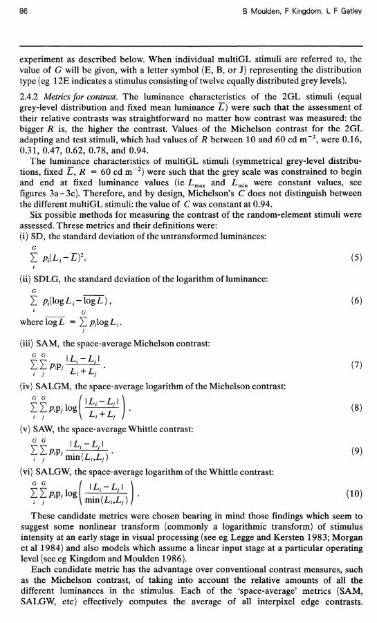
Figure 7a shows the results of experiment 3, illustrating the adaptive effect of two sets of adaptors each at five different mean luminances. The contrast of the adaptors (all of type 41; circles) producing the upper curve was 13.23 in SD units, and that of the adaptors (all of type 14E; squares) producing the lower curve was 9.3.

On the other hand, figure 6b (for subject FK) shows the results of experiment 2 for the same subject, illustrating the adaptive effect of a number of stimuli all having the same mean luminance (32 cd m~2) but each of which had one of a wide range of nominal SD contrast values.

Taking each of the data points of figure 7a in turn, it is possible to use the regression function shown in figure 6b (subject FK) to discover what value of SD at a mean luminance of 32 cd m~2 would have produced the same adapting effect as the stimuli represented in figure 7a. Each of the latter can then be described in terms of their equivalent nominal contrast at a mean luminance of 32 cd m~2. This value (Sc) is thus the SD value at a mean luminance of 32 cd m - 2 that would have produced the same adapting effect as the stimuli at different mean luminances in experiment 3.


We then replotted the data of figure 7a, still as a function of mean luminance, but now with the ordinate in terms of this '32 cd m"2 equivalent' contrast value. We found that this gave exactly the same pattern as before if the ordinate was the logarithm of the equivalent contrast; rather than show this as a separate figure, we have merely superimposed the 'log equivalent contrast scale' upon the right-hand side of figure 7a.

Considering any one of the two parallel lines in 7a, it is clear that a linear increase in mean luminance produces a logarithmic (constant proportional) decrease in the equivalent adapting contrast. Given the equivalent adapting contrast of a stimulus at any one mean luminance it is thus possible to predict the equivalent adapting contrast of the same stimulus at any other mean luminance. The relationship is described by the expression:

logY2e = f [ l o g Y l e - / ; ( L l - L 2 ) ] , (ID where Yle is the equivalent nominal SD contrast of a given stimulus at one mean luminance (LI); Y2e is the^ equivalent nominal SD contrast of the same stimulus at another mean luminance (L2), and k is the slope of the effect of mean luminance.

Expression (11) simply says that the log of the new value is some function of the log of the original value minus the difference in the mean luminances multiplied by the slope. However, as it stands this expression is not general; it merely says that given one value on either of the two functions in figure 7a it is possible to calculate another value on the same function. It describes the effect of mean luminance on any given SD but does not take into account the actual value of that SD, and thus yields only relative, not absolute, values.

In order to make the expression general it is necessary to identify some determinate locus on the various functions that is equivalent for all values of SD: we chose to select the origin of each function. This is that value of mean luminance for which the adapting effect will be maximum for each SD, and it is easily identified.

First, it can be shown that for any given mean luminance the largest obtainable SD value results from the use of a 2GL stimulus. This is intuitively obvious since in this case all deviations from the mean value are at the maximum. Second, it is clear that this maximum value will occur when the range of luminances in the 2GL stimulus is twice

s* 5

0

FK 1.3

1.2

o

l . l

1.0 §

0.9 £

0.8

o 1.85

1.70

1.55 o

20 30 40 Mean luminance/cd m~

50 1.40

FK Distribution

• 41 • 14E

10

(b) 20 30 40

Mean luminance/cd m~ 50 10

(a) Figure 7. (a) Results of experiment 3. The effects of mean luminance on the adapting effect of two stimuli, distribution types 41 and 14E. Increasing mean luminance reduces the adapting effect of each in a similar, linear, fashion. Parallel lines fitted by eye. (b) Modelled data using digital Laplacian filter with a compressive nonlinearity (see text for details).


the mean luminance, because the mean luminance will be at its lowest possible physical value when the luminance of the lower of the two grey levels reaches its physical limit of zero. Finally, in a 2GL stimulus the SD is numerically equal to half that range, which in turn is equal to the mean luminance itself.

In short, the maximum SD value obtainable at any mean luminance is equal to the numerical value of that mean luminance. Conversely, the maximum effective contrast (Smax, in SD units) for any stimulus will occur when its mean luminance is equal to its nominal equivalent value for the SD (ie Se). Let this value of mean luminance be called Lmax. Then, letting the reference value Yle in equation (11) be Smax,, the effective adapting contrast of a stimulus of any equivalent nominal SD is given by:

logSe = log5 m a x . -0 .021(L m a x -L) , (12)

where L is the mean luminance in question, and 0.021 is the slope constant derived from figure 7a.

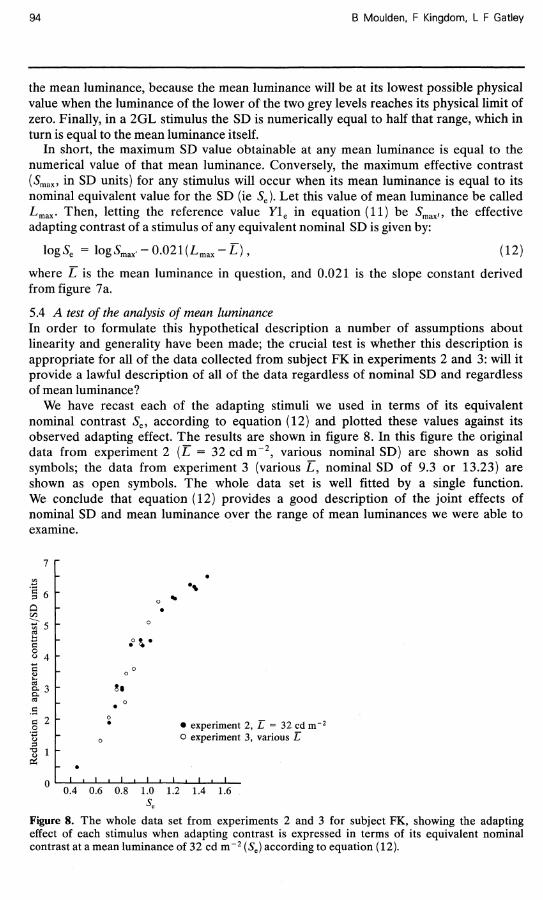
5.4 A test of the analysis of mean luminance In order to formulate this hypothetical description a number of assumptions about linearity and generality have been made; the crucial test is whether this description is appropriate for all of the data collected from subject FK in experiments 2 and 3: will it provide a lawful description of all of the data regardless of nominal SD and regardless of mean luminance?

We have recast each of the adapting stimuli we used in terms of its equivalent nominal contrast Sc, according to equation (12) and plotted these values against its observed adapting effect. The results are shown in figure 8. In this figure the original data from experiment 2 (L = 32 cd m~2, various nominal SD) are shown as solid symbols; the data from experiment 3 (various L, nominal SD of 9.3 or 13.23) are shown as open symbols. The whole data set is well fitted by a single function. We conclude that equation (12) provides a good description of the joint effects of nominal SD and mean luminance over the range of mean luminances we were able to examine.

• experiment 2, L = 32 cd m~2

o experiment 3, various L

' • ' • ' • ' • » • ' • i

0.4 0.6 0.8 1.0 1.2 1.4 1.6

Figure 8. The whole data set from experiments 2 and 3 for subject FK, showing the adapting effect of each stimulus when adapting contrast is expressed in terms of its equivalent nominal contrast at a mean luminance of 32 cd m~2 (5e) according to equation (12).

Q

t f 5


6 General discussion The results of the two main experiments described here show that the differential adaptive effects of the images of various compositions we used could be accounted for almost entirely by the contrast in those images, when contrast is defined as the standard deviation of luminance and calculated by means of equation (5). Taken together, the experiments involved different numbers of grey levels (2, 4, 6, 8, 10, 12, and 14), different distributions of grey-level proportions (equal, binomial, inverse binomial), and different luminance ranges, both for multi-grey-level stimuli (30 and 60 cd m~2) and for two-grey-level stimuli (10, 20, 30, 40, 50, and 60 cd m"2). Over all of these manipulations, the data were accounted for very successfully by the standard deviation expression for contrast, slightly less well so by the space-average Michelson contrast (SAM), and poorly by the five other candidate metrics tested.

As the above implies, when a subject adapted to each of two stimuli with different luminance distributions but very close SD values, the adaptive effects of those stimuli were almost invariably found to be very close. This shows that the particular nature of the distribution of intensities in the stimuli (ie number of grey levels, range of grey scale, shape of grey-level distribution) was not important in determining their adaptive power.

6.1 Is it possible to discriminate between the SAM metric and the SD metric ? The results for both observers showed that one other metric besides the SD, namely the space-average Michelson contrast or SAM, could also provide a relatively good description of the data for 2GL and multiGL adapting conditions collectively. Both metrics offer a good engineering approximation, accounting for more than 90% of the variance, but since each is predicated upon a different implicit assumption about visual function it is important on theoretical grounds to try to distinguish between them.

The fact that the data for both subjects, although individually different, were so well fitted by both metrics, first led us to fear that there might be some simple mathematical relationship between the two metrics, resulting perhaps in their being linearly related over at least some part of their range. In order to check this we calculated SD and SAM values for a number of distribution types and then plotted one against the other in order to examine the relationship between them. An example of such a plot is shown in figure 9.

30 r /

/ * 25 r /

20 L /

Stimulus • 2GL A multiGL type B • multiGL type E • multiGL type I

o k L j i i i i — i — i — i — i — i 0 10 20 30 40 50

SAM Figure 9. The relationship between the space-average Michelson contrast (SAM) and the standard deviation of the untransformed luminances (SD) as measures of contrast for various exemplars of the luminance distribution types in experiments 2 and 3.


Note first the obvious fact that for 2GL stimuli there is a linear relationship between the SAM and SD metrics. This is to be expected: with only two luminance values it is clear that both will simply increase directly with the range of the two values. The more interesting and important fact, however, is that although there is also a linear relationship between the two metrics for multiGL stimuli, the slope of the functions is different from that for the 2GL stimuli.

This has the following implications. Consider any 2GI7multiGL pair with the same contrast as measured by the metric SD; for this pair the corresponding value of the SAM metric is higher for the 2GL stimulus than for the multiGL stimulus. Consequently the SAM metric predicts a higher adaptive effect for the 2GL stimulus than for the multiGL stimulus, whereas the SD metric predicts that the two will have the same adaptive effect.

Another way of putting this is to say that if the SD metric is correct then when the data are plotted according to the SAM metric the rate of growth of the adaptive effect will appear to be different (higher) for the 2GL stimuli than for the multiGL stimuli; the two will be indistinguishable when plotted in terms of SD. On the other hand, if the SAM metric is correct then when the data are plotted according to SD the rate of growth of the adaptive effect will appear to be different (lower) for the 2GL stimuli than for the multiGL stimuli. The two will be indistinguishable when plotted in terms of the SAM metric.

In order to choose between these two possibilities we calculated separate regression functions for the 2GL data and the multiGL data, when those data were cast in terms of either SD or SAM.

The dashed (G = 2) and dotted (G > 2) lines in the two graphs in figure 6a are the regression functions obtained for subjects LG and FK, with the data plotted in terms of SAM. In both cases the two regression lines are significantly different from each other, but in the case of the SD measure the functions describing the two classes of data are so similar to the regression line calculated for the data as a whole (the two solid lines in figure 6a) that there was no point in drawing them separately. Moreover, the direction of the errors in prediction in the case of the SAM measure is that expected on the basis of the argument presented above: the SAM metric overestimates the adaptive effect of the 2GL stimuli compared with the multiGL stimuli.

This closer analysis of the regression functions leads us to conclude that, despite the similarity in the overall coefficients of determination, the precision of prediction for the SAM and the SD metrics can be distinguished: the SD metric gives the better description of the data.

These results suggest that for displays of the kind used here, a definition of contrast in which the standard deviation of luminance in the stimulus is computed is highly successful and is preferable to the other candidate metrics we devised and examined.

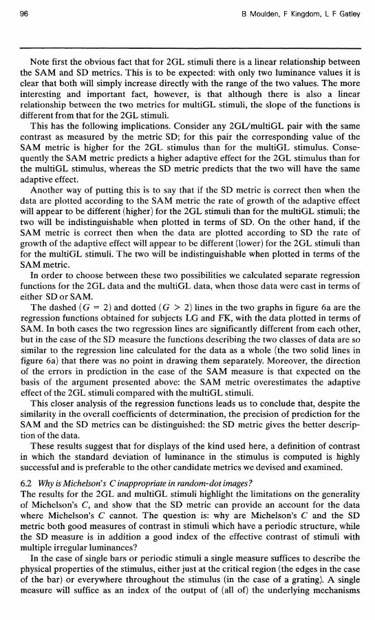
6.2 Why is Michelson's C inappropriate in random-dot images ? The results for the 2GL and multiGL stimuli highlight the limitations on the generality of Michelson's C, and show that the SD metric can provide an account for the data where Michelson's C cannot. The question is: why are Michelson's C and the SD metric both good measures of contrast in stimuli which have a periodic structure, while the SD measure is in addition a good index of the effective contrast of stimuli with multiple irregular luminances?

In the case of single bars or periodic stimuli a single measure suffices to describe the physical properties of the stimulus, either just at the critical region (the edges in the case of the bar) or everywhere throughout the stimulus (in the case of a grating). A single measure will suffice as an index of the output of (all of) the underlying mechanisms


involved: for example, the response of elongated receptive fields is proportional to the contrast of the stimulus driving them.

In the case of stimuli with multiple irregular luminances what is required is some measure that will reflect the average of a number of responses of different magnitudes at different locations in the image. No single local value represents the average global response; some intrinsically global measure is required. But why is the SD better than, say, the space-average Michelson contrast? The beginnings of an answer to this question would be provided if it were possible to show that the SD correlates more strongly than the SAM with the average magnitude of the internal response variable that might encode contrast.

6.3 Can the success of the SD metric be explained by computational modelling? We assume, obviously, that apparent contrast is some function of the cortical response variable; we further assume that this in turn is some function of the retinal ganglion cell response variable. We have modelled the latter by using a balanced 3 x 3 digital Laplacian operator. The central cell had a weighting of +8 and each of the eight surrounding cells had a weighting of - 1 . (In more sophisticated modelling of this type, difference-of-Gaussian or DOG functions are used, but the crude convolution mask that we use gives an approximation that is perfectly adequate for our present purposes.) Cell size was set to be equal to 1 pixel. Since at the viewing distance used each pixel subtended about 5 min visual angle, the overall diameter of this mask was about 15 min; this is almost identical to the overall diameter of the smallest DOG filter proposed by Wilson and Bergen (1979). Using a Monte Carlo simulation procedure, we repeatedly convolved the mask with samples drawn from exemplars of the stimulus type in question. We took the mean of all convolution responses from all the samples and defined this mean as the average convolution product for that particular stimulus.

Each of these computations was performed twice, once with the untransformed luminance values of the stimuli and once with the transformed values. In the case of the transformed luminances we used a saturating nonlinear function of the form:

where r(i) is the response to light of intensity /, rmax is the maximum response, and H represents the light intensity at which half the maximum response is produced. This is a version of the Michaelis-Menton equation which has been successfully used to model retinal response (eg see Hood and Finkelstein 1979; Morgan et al 1984; Naka and Rushton 1966; Toet et al 1988).

To summarise: we convolved a digital Laplacian filter with either the raw or the transformed luminance values to calculate, for each stimulus, two average convolution products. We then calculated the correlation between each of these average values and the corresponding SD and SAM values for each stimulus.

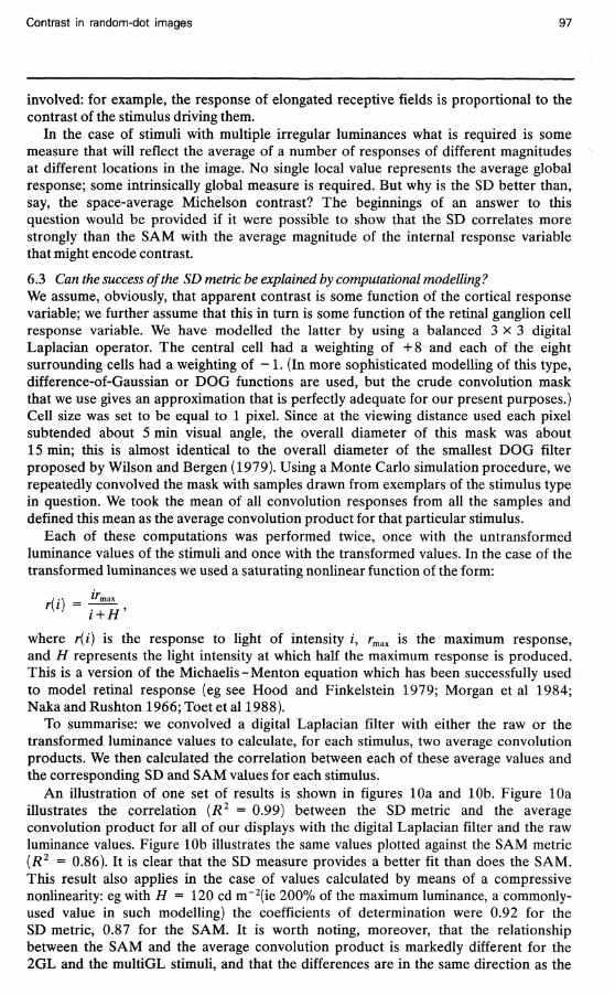
An illustration of one set of results is shown in figures 10a and 10b. Figure 10a illustrates the correlation (R2 = 0.99) between the SD metric and the average convolution product for all of our displays with the digital Laplacian filter and the raw luminance values. Figure 10b illustrates the same values plotted against the SAM metric {R2 = 0.86). It is clear that the SD measure provides a better fit than does the SAM. This result also applies in the case of values calculated by means of a compressive nonlinearity: eg with H = 120 cd m~2(ie 200% of the maximum luminance, a commonly-used value in such modelling) the coefficients of determination were 0.92 for the SD metric, 0.87 for the SAM. It is worth noting, moreover, that the relationship between the SAM and the average convolution product is markedly different for the 2GL and the multiGL stimuli, and that the differences are in the same direction as the


differences in the description of the data by the SAM that we described earlier. In fact these differences, although in the same direction, are slightly more marked in the model output than they were in the data, but this is simply a consequence of the particular implementation we used. The model could be arbitrarily tuned to make the agreement with the data more exact, but we have not attempted to optimise the modelling (by using different averaging procedures or different values of H, for example) because these results, obtained with the minimum number of assumptions, are sufficient for our present purposes.

Notice that these results hold whether or not a nonlinear compressive transform of input luminances is used (although note that in our modelling of the effects of mean luminance, below, a compressive tranform is essential). This is of some theoretical importance. In previous publications (Kingdom and Moulden 1986; Moulden and Kingdom 1987, 1988) in which we modelled the detectability of line signals in visual noise, we found that use of the standard deviation of the untransformed luminances led to a good description of the data, and specifically commented on this fact since it was at odds with other studies (such as those cited earlier) that had shown the need for a compressive nonlinearity to account for the brightness response in humans.

It is clear from the results of the modelling above that it is probably best to regard the SD merely as a correlate of the internal response variable, rather than as a direct measure of it. Now although the correlate may not require a transform, it is perfectly possible that the direct measure of which it is an index (here the output of modelled ganglion cell receptive fields) may require such a transform. The fact that it is possible to model data without the need for a compressive transform does not necessarily imply that no such transformation occurs in the visual system: there may be a general lesson to be learned from this observation.

The main conclusion from the modelling, then, is that the SD correlates more strongly than the SAM with the average convolution products of a Laplacian filter and our displays. We speculate that this may account for the descriptive power of the SD metric: it is a computationally convenient correlate of these convolution products, which in turn may be a good description of the output of retinal ganglion cells. This is not to imply that we believe the retina to be the site of the adaptation we measured,

240

- 192

144

Stimulus • 2GL • multiGl

0 5 10 15 20 25 30 Adapting contrast/SD units

0

(b)

0.1 0.2 0.3 0.4 0.5 Adapting contrast/SAM units

(a) Figure 10. The average convolution product of the untransformed luminance values of the stimuli used in the experiments and a digital Laplacian filter as described in the text, (a) as a function of the standard deviation of the untransformed luminances (SD) metric, (b) as a function of the space-average Michelson contrast (SAM).


merely that since retinal output becomes cortical input it is a reasonable basis for the modelling. Because of the small size of the pixels compared with the magnitude of spontaneous eye movements to be expected even when the subject is ostensibly fixating, it is most unlikely that the adaptation we measured could be retinal in origin. The question could be settled empirically by repeating some of the above observations with a procedure in which adaptation and test stimuli are seen with different eyes. Blakemore and Campbell (1969) demonstrated that the threshold elevation phenomenon which occurs after prolonged exposure to a high-contrast grating transfers readily from one eye to the other. They inferred from this that the adaptation occurred at some locus central to the point of binocular fusion; we would expect the same result with stimuli of the kind used here.

6.4 How can the effects of mean luminance be taken into account? We now turn to a discussion of the effects of mean luminance. Once again we used the digital Laplacian filter described in the section above to calculate the average convolution products of the stimuli used in experiment 3. Since the SD value for any distribution of grey-level values remains the same if a constant is added to each value it was clear that the convolution products calculated with the untransformed luminance values would not discriminate between different mean luminances, so we used the compressive transform described above, again with H set to 200% of the mean luminance.

Figure 7b shows the result of this modelling. The logarithm of mean filter output declines linearly with an increase in mean luminance, and the functions for the 41 (nominal SD 13.23) and the 14E (nominal SD 9.3) stimuli are parallel. Compare the results of this modelling with the data of figure 7a: although the overall slopes of the two are different (this depends upon the precise value chosen for H in the nonlinear transform) the similarity between the two sets of functions further confirms the relationship between the SD measure and the modelled internal response variable.

6.5 What is the relationship between SD and the Fourier spectrum ? We measured the Fourier power spectra for samples of all of our multi-grey-level stimuli using a FORTRAN implementation of an FFT algorithm (IEEE 1979). We found no differences in the shape of the power spectra, only in their average amplitude. This is to be expected since the spectrum is determined only by the autocorrelation function of the stimuli, which is the same whatever the intensity distribution. The measure of the intensity parameter of noise patterns is the noise power density, which is determined solely by the variance and the pixel size. Since pixel size was constant for all our patterns, the SD therefore represents a computationally convenient measure of the average power of the stimuli. For this reason the standard deviation should reflect the average response of any of the range of bandpass filters that are sensitive to the luminance variation in the stimuli. Viewed in this light the success of the SD metric in predicting the average convolution product in the filter modelling described above is therefore not surprising.

6.6 Possible development It is commonly assumed that the effective contrast of a stimulus is inversely proportional to its mean luminance; this is implicit, for example, in the Michelson expression where the denominator is twice the mean luminance. Effective contrast would thus be expected to be a curvilinear function of mean luminance; but both in our data and in our modelling the function is approximately linear. As a result [see equation (12)] the effect of mean luminance appears to be a subtractive, rather than a dividing, function. This rather implausible implication is almost certainly a consequence of the limited range of mean luminances we were able to study with our apparatus. It would be useful


to repeat the experiment over a wider range in order to discover a more general expression than equation (12) to describe the effects of mean luminance.

It would also be useful to extend the investigation to include asymmetrical luminance distributions in order to demonstrate that the use of only symmetrical distributions in this investigation did not significantly affect the results. By generating stimuli with the value of P in equation (4) set to more or less than 0.5, the binomial luminance distribution can be skewed to the left or right respectively. Similar asymmetries can be introduced for the inverse binomial conditions we investigated.

A further test of the generality of the measure might be provided by a contrast discrimination procedure: are two stimuli of different grey-level distribution but identical SD contrast equally discriminable from a comparison stimulus? The performance of unadapted subjects in the experiments described here suggests that contrast matching of two similarly composed (2GL) random-element stimuli can be accurately performed. However, the task of matching the contrast of the multi-grey-level stimuli of various compositions described in this paper is likely to be difficult.

Finally, we have recently shown that in random-dot kinematogram pairs of various luminance distributions the magnitude of Dmin (the minimum displacement of correlated elements whose direction can reliably be detected) (Braddick 1980) varies according to contrast when contrast is expressed in terms of SD; this strengthens our belief that the SD is a useful general measure of contrast in such images.

Acknowledgements. This work was supported in part by Grant ER1/9/4/2035/052 from the Ministry of Defence, UK, and in part by Grant GR/D 89165 from the Science and Engineering Council of Great Britain under the auspices of the Image Interpretation Initiative.

References Blakemore C, Campbell F W, 1969 "On the existence of neurones in the human visual system

selectively sensitive to the orientation and size of retinal images" Journal of Physiology (London) 203 237-260

Blakemore C, Muncey J P J, Ridley R M, 1971 "Perceptual fading of a stabilized cortical image" Nature (London) 233 204 - 205

Blakemore C, Muncey J P J, Ridley R M, 1973 "Stimulus specificity in the human visual system" Vision Research 13 1915-1931

Braddick O L, 1980 "Low-level and high-level processes in apparent motion" Philosophical Transactions of the Royal Society of London, Series B 2 90 137-151

Burgess A E, Wagner R F, Jennings R J, Barlow H B , 1981 "Efficiency of human visual signal discrimination" Science 214 93 - 94

Burr D C, Ross J, Morrone M C, 1985 "Local regulation of luminance gain" Vision Research 25 717-727

Campbell F W, Green D, 1965 "Optical and retinal factors affecting visual resolution" Journal of Physiology (London) 187 427 - 436

Campbell F W, Robson J G, 1968 "Application of Fourier analysis to the visibility of gratings" Journal of Physiology (London) 197 551 - 556

Georgeson M A, 1985 "The effect of spatial adaptation on perceived contrast" Spatial Vision 1 103-112

Hamerly J R, Quick R F, Reichert T A, 1977 "A study of grating contrast judgement" Vision Research 17 201-207

Hood D C, Finkelstein M A, 1979 "Comparison of changes in sensitivity and sensation: implications for the response-intensity function of the human scotopic system" Journal of Experimental Psychology 5391-405

IEEE, 1979 Programs for Digital Signal Processing edited by the Digital Signal Processing Committee, IEEE Acoustics, Speech and Signal Processing Society (New York: IEEE Press)

Kingdom F, Moulden B, 1986 "Digitized images: what type of grey scale should one use?" Perception 15 17-25

Legge G E, Kersten D, 1983 "Light and dark bars; contrast discrimination" Vision Research 23 473-483

Mayhew J E W , Frisby J P, 1978 "Suprathreshold contrast perception and complex random textures" Vision Research 18 895-897


Michelson A A, 1927 Studies in Optics (Chicago, IL: University of Chicago Press) Morgan M J, Mather G, Moulden B, Watt R J, 1984 "Intensity-response nonlinearities and the

theory of edge localization" Vision Research 24 713-719 Moulden B, Kingdom F, 1987 "Effect of the number of grey levels on the detectability of a simple

line signal in visual noise" Spatial Vision 2 61-77 Moulden B, Kingdom F, 1988 "Effect of pixel width, display width, and horizontal resolution on

the detection of a simple vertical line signal in visual noise" Perception & Psychophysics 43 592-598

Moulden B, Kingdom F, 1989 "An orientation anisotropy in induced brightness" Perception 18 pp 703-713

Nagaraja N S, 1964 "Effect of luminance noise on contrast thresholds" Journal of the Optical Society of America 54950-955

Naka K I, Rush tonWAH, 1966 "S-potentials from luminosity units in the retina of fish (cyprinidae)" Journal of Physiology (London) 185587-599

Quick R F, Hamerly J R, Reichert T A, 1976 "The absence of a measurable critical band at low suprathreshold contrasts" Vision Research 16351-355

Rayleigh J W S, 1889 "On the limit to interference when light is radiated from moving molecules" Philosophical Magazine 27 298 - 304

Stanley P A, 1987 The Detection of Disc Targets in Broadband Noise report JS10804, British Aerospace PLC, Sowerby Research Centre, Filton, Bristol, UK

Stromeyer C F, Julesz B, 1972 "Spatial-frequency masking in vision: critical bands and spread of masking" Journal of the Optical Society of America 62 1221-1232

Swensson R G, Judy P F, 1981 "Detection of noisy visual targets: Models for the effects of spatial uncertainty and signal-to-noise ratio" Perception & Psychophysics 29 521 - 534

Toet A, Snippe H P, Koenderink J J, 1988 "Effects of blur and eccentricity on differential spatial displacement discrimination" Vision Research 28 535-554

Tolhurst D J, 1972 "Adaptation to square-wave gratings: inhibition between spatial frequency channels in the human visual system" Journal of Physiology (London) 226 231 - 248

Whittle P, 1986 "Increments and decrements: luminance discrimination" Vision Research 26 1677-1691

Wilson H R, Bergen J R, 1979 "A four mechanism model for threshold spatial vision" Vision Research 1919-32

The standard deviation of luminance as a metric for...

Documents

Transcript of The standard deviation of luminance as a metric for...