THE SPITZER c2d SURVEY OF LARGE, NEARBY ...authors.library.caltech.edu/18053/1/HARapj07b.pdfTHE...
25
THE SPITZER c2d SURVEY OF LARGE, NEARBY, INTERSTELLAR CLOUDS. IX. THE SERPENS YSO POPULATION AS OBSERVED WITH IRAC AND MIPS Paul Harvey, 1 Bruno MerI ´ ı ´ n, 2 Tracy L. Huard, 3 Luisa M. Rebull, 4 Nicholas Chapman, 5 Neal J. Evans II, 1 and Philip C. Myers 3 Received 2007 January 29; accepted 2007 April 1 ABSTRACT We discuss the combined IRAC/MIPS c2d Spitzer Legacy observations of the Serpens star-forming region. We describe criteria for isolating bona fide YSOs from the extensive background of extragalactic objects. We then discuss the properties of the resulting high-confidence set of 235 YSOs. An additional 51 lower confidence YSOs outside this area are identified from the MIPS data and 2MASS photometry. We present color-color diagrams to compare our observed source properties with those of theoretical models for star/disk /envelope systems and our own modeling of the objects that are well represented by a stellar photosphere plus circumstellar disk. These objects exhibit a wide range of disk properties, from many with actively accreting disks to some with both passive disks and even possibly debris disks. The YSO luminosity function extends down to at least a few times 10 3 L or lower. The lower limit may be set more by our inability to distinguish YSOs from extragalactic sources than by the lack of YSOs at very low luminosities. We find no evidence for variability in the shorter IRAC bands between the two epochs of our data set, t 6 hr. A spatial clustering analysis shows that the nominally less evolved YSOs are more highly clustered than the later stages. The background extragalactic population can be fitted by the same two-point correlation function as seen in other extragalactic studies. We present a table of matches between several previous infrared and X-ray studies of the Serpens YSO population and our Spitzer data set. The clusters in Serpens have a very high surface density of YSOs, primarily with SEDs suggesting extreme youth. The total number of YSOs, mostly Class II, is greater outside the clusters. Subject headingg s: infrared: general Online material: machine-readable tables 1. INTRODUCTION The Serpens star-forming cloud is one of five such large clouds selected for observation as part of The Spitzer Legacy project ‘‘From Molecular Cores to Planet-forming Disks’’ (c2d; Evans et al. 2003). Previous papers in this series have described the observational results in the Serpens cloud as seen with IRAC ( Harvey et al. 2006, hereafter Paper II) and MIPS ( Harvey et al. 2007), as well as some of the other clouds (Jorgensen et al. 2006; Rebull et al. 2007). In this paper we examine how the combination of the IRAC and MIPS data together with other published results on this region can be used to find and charac- terize a highly reliable catalog of young stellar objects ( YSOs) in the surveyed area. With the combination of broad wavelength coverage and amazing depth of Spitzer’s sensitivity we are able both to probe to extremely low luminosity limits for YSOs and to cover a very wide range in dust emission, both in optical depth and in range of emitting temperatures. The Spitzer wavelength region is particularly well tuned for sensitivity to dust at temper- atures appropriate for solar systemY size disks around young stars. The region of the Serpens cloud mapped in our survey is an area rich in star formation. Eiroa et al. (2007) have extensively reviewed studies at a variety of wavelengths of this area. There is evidence from previous observations of strong clustering (Testi et al. 2000; Testi & Sargent 1998), dense submillimeter cores (Casali et al. 1993; Enoch et al. 2006b), and high-velocity out- flows (Ziener & Eisloffel 1999; Davis et al. 1999). Pre-Spitzer infrared surveys of the cloud have been made by IRAS ( Zhang et al. 1988a, 1988b) and the Infrared Space Observatory (ISO; Kaas et al. 2004; Djupvik et al. 2006), as well as the pioneering ground-based surveys that first identified it as an important region of star formation (Strom et al. 1976). Using MIPS and all four bands of IRAC, the c2d program has mapped a 0.85 deg 2 portion of this cloud that includes a very well studied cluster of infrared and submillimeter sources ( Eiroa & Casali 1992; Hogerheijde et al. 1999; Hurt & Barsony 1996; Harvey et al. 1984; Testi & Sargent 1998). At its distance of 260 10 pc (Straizys et al. 1996) this corresponds to an area of about 2:5 ; 9 pc. In Paper II we identified at least two main centers of star formation as seen by Spitzer in this cloud, which we referred to as clusters A and B. Cluster A is the very well studied grouping also commonly re- ferred to as the Serpens core. Cluster B was the subject of a recent multiwavelength study by Djupvik et al. (2006), who referred to it as the Serpens G3 Y G6 cluster. The 235 YSOs with high signal-to-noise ratio (S/N) that we have cataloged constitute a sufficiently large number that we can examine statistically the numbers of objects in various evolu- tionary states and the range of disk properties for different classes of YSOs. We characterize the circumstellar material with color- color diagrams that allow comparison with other recent studies of star-forming regions, and we model the energy distributions of the large number of YSOs that appear to be star+circumstellar disk systems. We are able to construct the YSO luminosity func- tion for Serpens since we have complete spectral coverage for all the sources over the range of wavelengths where their luminosity 1 Astronomy Department, University of Texas at Austin, Austin, TX 78712- 0259; [email protected], [email protected]. 2 Research and Scientific Support Department, ESTEC (ESA), 2200 AG Noordwijk, Netherlands; and Leiden Observatory, Leiden University, 2300 RA Leiden, Netherlands; [email protected]. 3 Smithsonian Astrophysical Observatory, Cambridge, MA 02138; thuard@ cfa.harvard.edu, [email protected]. 4 Spitzer Science Center, Pasadena, CA 91125; [email protected]. 5 Astronomy Department, University of Maryland, College Park, MD 20742; [email protected]. A 1149 The Astrophysical Journal, 663:1149 Y 1173, 2007 July 10 # 2007. The American Astronomical Society. All rights reserved. Printed in U.S.A.
Transcript of THE SPITZER c2d SURVEY OF LARGE, NEARBY ...authors.library.caltech.edu/18053/1/HARapj07b.pdfTHE...

THE SPITZER c2d SURVEY OF LARGE, NEARBY, INTERSTELLAR CLOUDS. IX.THE SERPENS YSO POPULATION AS OBSERVED WITH IRAC AND MIPS
Paul Harvey,1
Bruno MerI´ın,
2Tracy L. Huard,
3Luisa M. Rebull,
4Nicholas Chapman,
5
Neal J. Evans II,1
and Philip C. Myers3
Received 2007 January 29; accepted 2007 April 1
ABSTRACT
We discuss the combined IRAC/MIPS c2d Spitzer Legacy observations of the Serpens star-forming region. Wedescribe criteria for isolating bona fide YSOs from the extensive background of extragalactic objects.We then discussthe properties of the resulting high-confidence set of 235YSOs. An additional 51 lower confidence YSOs outside thisarea are identified from the MIPS data and 2MASS photometry. We present color-color diagrams to compare ourobserved source properties with those of theoretical models for star/disk/envelope systems and our own modeling ofthe objects that are well represented by a stellar photosphere plus circumstellar disk. These objects exhibit a widerange of disk properties, from many with actively accreting disks to some with both passive disks and even possiblydebris disks. TheYSO luminosity function extends down to at least a few times 10�3 L� or lower. The lower limit maybe set more by our inability to distinguish YSOs from extragalactic sources than by the lack of YSOs at very lowluminosities. We find no evidence for variability in the shorter IRAC bands between the two epochs of our data set,�t � 6 hr. A spatial clustering analysis shows that the nominally less evolved YSOs are more highly clustered thanthe later stages. The background extragalactic population can be fitted by the same two-point correlation function asseen in other extragalactic studies. We present a table of matches between several previous infrared and X-ray studiesof the Serpens YSO population and our Spitzer data set. The clusters in Serpens have a very high surface density ofYSOs, primarily with SEDs suggesting extreme youth. The total number of YSOs, mostly Class II, is greater outsidethe clusters.
Subject headinggs: infrared: general
Online material: machine-readable tables
1. INTRODUCTION
The Serpens star-forming cloud is one offive such large cloudsselected for observation as part of The Spitzer Legacy project‘‘From Molecular Cores to Planet-forming Disks’’ (c2d; Evanset al. 2003). Previous papers in this series have described theobservational results in the Serpens cloud as seen with IRAC(Harvey et al. 2006, hereafter Paper II) andMIPS (Harvey et al.2007), as well as some of the other clouds (Jorgensen et al.2006; Rebull et al. 2007). In this paper we examine how thecombination of the IRAC and MIPS data together with otherpublished results on this region can be used to find and charac-terize a highly reliable catalog of young stellar objects (YSOs) inthe surveyed area. With the combination of broad wavelengthcoverage and amazing depth of Spitzer’s sensitivity we are ableboth to probe to extremely low luminosity limits for YSOs and tocover a very wide range in dust emission, both in optical depthand in range of emitting temperatures. The Spitzer wavelengthregion is particularly well tuned for sensitivity to dust at temper-atures appropriate for solar systemYsize disks around young stars.
The region of the Serpens cloud mapped in our survey is anarea rich in star formation. Eiroa et al. (2007) have extensivelyreviewed studies at a variety of wavelengths of this area. There is
evidence from previous observations of strong clustering (Testiet al. 2000; Testi & Sargent 1998), dense submillimeter cores(Casali et al. 1993; Enoch et al. 2006b), and high-velocity out-flows (Ziener & Eisloffel 1999; Davis et al. 1999). Pre-Spitzerinfrared surveys of the cloud have been made by IRAS (Zhanget al. 1988a, 1988b) and the Infrared Space Observatory (ISO;Kaas et al. 2004; Djupvik et al. 2006), as well as the pioneeringground-based surveys that first identified it as an important regionof star formation (Strom et al. 1976). Using MIPS and all fourbands of IRAC, the c2d program has mapped a 0.85 deg2 portionof this cloud that includes a very well studied cluster of infraredand submillimeter sources (Eiroa & Casali 1992; Hogerheijdeet al. 1999; Hurt & Barsony 1996; Harvey et al. 1984; Testi &Sargent 1998). At its distance of 260� 10 pc (Straizys et al.1996) this corresponds to an area of about 2:5 ; 9 pc. In Paper IIwe identified at least two main centers of star formation as seenby Spitzer in this cloud, which we referred to as clusters A and B.Cluster A is the very well studied grouping also commonly re-ferred to as the Serpens core. Cluster Bwas the subject of a recentmultiwavelength study by Djupvik et al. (2006), who referred toit as the Serpens G3YG6 cluster.
The 235 YSOs with high signal-to-noise ratio (S/N) that wehave cataloged constitute a sufficiently large number that we canexamine statistically the numbers of objects in various evolu-tionary states and the range of disk properties for different classesof YSOs. We characterize the circumstellar material with color-color diagrams that allow comparison with other recent studiesof star-forming regions, and we model the energy distributionsof the large number of YSOs that appear to be star+circumstellardisk systems. We are able to construct the YSO luminosity func-tion for Serpens since we have complete spectral coverage for allthe sources over the range of wavelengths where their luminosity
1 Astronomy Department, University of Texas at Austin, Austin, TX 78712-0259; [email protected], [email protected].
2 Research and Scientific Support Department, ESTEC (ESA), 2200 AGNoordwijk, Netherlands; and Leiden Observatory, Leiden University, 2300 RALeiden, Netherlands; [email protected].
3 Smithsonian Astrophysical Observatory, Cambridge, MA 02138; [email protected], [email protected].
4 Spitzer Science Center, Pasadena, CA 91125; [email protected] AstronomyDepartment, University of Maryland, College Park,MD20742;
A
1149
The Astrophysical Journal, 663:1149Y1173, 2007 July 10
# 2007. The American Astronomical Society. All rights reserved. Printed in U.S.A.
is emitted, and we are able to characterize the selection effectsinherent in the luminosity function from comparison with thepublicly available and significantly deeper SWIRE survey(Surace et al. 20046). We find that the population of YSOs ex-tends down to luminosities below 10�2 L�, and we discuss thesignificance of this population. Our complete coverage in wave-length and luminosity space also permits us to discuss the spatialdistribution of YSOs to an unprecedented completeness level.We note also that, unlike the situation discussed by Jorgensenet al. (2006) for Perseus, in Serpens there do not appear to beany very deeply embedded YSOs that are not found by our YSOselection criteria.
In x 2 we briefly review the observational details of this pro-gram, and then in x 3 we describe in detail the process by whichwe identify YSOs and eliminate background contaminants. Inx 4 we describe a search for variability in our data set. We com-pare our general results on YSOs with those of earlier studies ofthe Serpens star-forming region in x 5.We discuss in x 6 the YSOluminosity function in Serpens and, in particular, the low end ofthis function. We next analyze the spatial distribution of starformation in the surveyed area and compare it to the distribu-tion of dust extinction as derived from our observations in x 7.In x 8 we construct several color-color diagrams that characterizethe global properties of the circumstellar material and showmodeling results for a large fraction of our YSOs that appearto be star+disk systems. Finally, x 9 discusses several specificgroups of objects including the coldest YSOs and a previouslyidentified ‘‘disappearing’’ YSO. We also mention several obvi-ous high-velocity outflows from YSOs that will certainly be thesubject of further study.
2. OBSERVATIONS
The parameters of our observations have already been de-scribed in detail in Paper II for IRAC and in a companion study(Harvey et al. 2007) for MIPS. We summarize here some of theissues most relevant to this study.
We remind the reader that the angular resolution of the Spitzerimaging instruments varies widely with wavelength, since Spitzeris diffraction limited longward of k � 10 �m. In the shorter IRACbands the spatial resolution is of order 200, while from 24 to 160�m,it goes from roughly 500 to 5000. The area chosen for mappingwas defined by the AV > 6 contour in the extinction map ofCambresy (1999) and by practical time constraints (Evans et al.2003). With the exception of a small area of 0.04 deg2 on thenortheast edge of the IRAC map, all of the area mapped withIRAC was also covered with MIPS at both 24 and 70 �m, andmost of it at 160 �m. As described by Harvey et al. (2007), somesubstantial additional areawas observedwithMIPSwithoutmatch-ing IRAC observations. In this paper we restrict our attention toonly the area that was observed from 3.6 to 70 �m, 0.85 deg2.This entire region was observed from 3.6 to 24 �m at two ep-ochs, with a time separation of several hours to several days, butat only one epoch at 70 �m. We also specifically do not includethe 160 �m observations in our discussion because they did notcover the entire area and because most of the YSOs in Serpensare too closely clustered to be distinguishable in the large beamof the 160 �m data. Harvey et al. (2007) discuss briefly the ex-tended 160 �m emission in this region and the four pointlikesources found at 160 �m. Figure 1 shows the entire area mappedwith all four IRAC bands and MIPS at 24 and 70 �m and alsoindicates the locations of several areas mentioned in the text.
In addition to this area of the Serpens cloud defined by rela-tively high AV , we also observed small off-cloud regions aroundthe molecular cloud with relatively low AV in order to determinethe background star and galaxy counts. The area of combinedIRAC/MIPS coverage of these off-cloud regions, however, wasrelatively small and so these observations are not discussed fur-ther in this paper. As detailed below, we have used the much6 Available at http://ssc.spitzer.caltech.edu/ legacy/.
Fig. 1.—Three-color image of the area mapped in Serpens. The color map-ping is blue, green, and red for 4.5, 8.0, and 24 �m, respectively. The locationsof cluster A (core cluster), cluster B (Serpens G3YG6 cluster), and VV Ser areindicated.
HARVEY ET AL.1150 Vol. 663

larger and deeper SWIRE (Surace et al. 2004) survey to under-stand the characteristics of the most serious background con-taminants in our maps, the extragalactic objects.
3. YSO SELECTION
Paper II described a process for classifying infrared objectsinto several categories: those whose energy distributions couldbe well fitted as reddened stellar photospheres, those that hada high likelihood of being background galaxies, and those thatwere viable YSO candidates. We have refined this process bycombining MIPS and IRAC data together, as well as by produc-ing an improved comparison catalog from the SWIRE (Suraceet al. 2004) survey, trimmed as accurately as possible to the c2dsensitivity limits. As shownby the number counts versusWainscoatmodels of the Galactic background toward Serpens in Paper II,nearly all the sources observed in our survey are likely to be back-ground stars. Because of the high sensitivity of IRAC channels 1and 2 relative to both the TwoMicron All Sky Survey (2MASS)and IRAC channels 3 and 4, most of the more than 200,000sources extracted from our Serpens data set do not have enoughspectral coverage for any reliable classification algorithm. Inparticular, ‘‘only’’ 34,000 sources had enough spectral informa-tion from a combination of 2MASS and IRAC data to permit atest for consistency with a stellar photosphere plus extinctionmodel, and nearly 32,000 of these objects were classified asreddened stellar photospheres. These normal stellar objects arenot considered further in our discussion and are not plotted onthe various color and magnitude diagrams. The details of thisclassification process and the criteria for fitting are described indetail by Evans et al. (2007).
In order to pursue the classification process for YSOs beyondthat described in Paper II, we added one more step to the dataprocessing described there. This final step was ‘‘band filling’’ thecatalog to obtain upper limits or low-S/N detections of objects thatwere not found in the original source extraction processing.This step is described in detail in the delivery documentation forthe final c2d data delivery (Evans et al. 2007). In short, however,it involved fixing the position of the source during an extractionat the position of an existing catalog source and fitting the imagedata at that fixed position for two parameters, a background leveland source flux, assuming that it was a point source. For thisprocessing step, the fluxes of all the originally extracted sourceswere subtracted from the image first. In the case of the data dis-cussed in this paper, the most important contribution of this band-filling step is to give us flux estimates for the YSO candidates andextragalactic candidates at 24 �m. Because our knowledge ofthe true point-spread function (PSF) is imperfect and becausethe 24 �m PSF is so much larger than the IRAC ones, it was alsonecessary to examine these results carefully to be sure a band-filled 24 �mflux was not simply the poorly subtracted wings of anearby bright source that, in fact, completely masked the sourcebeing band filled. For the purposes of this paper, all upper limitsare given as 5 � values.
Three of the sources eventually selected as YSOs by the pro-cess described below had 24 �m fluxes that were obviously sat-urated. These are the objects in Table 2 below numbered 127,137, and 182. For these three objects we derived the 24 �m fluxfrom a fit to the wings of the source profiles, rather than a fit to thewhole profile as is done by the standard c2d source extraction.
3.1. Constructing a Control Catalog from DeepExtragalactic SWIRE Observations
We use the IRAC and MIPS images of the ELAIS N1 fieldobtained by the SWIRE team as a control field for understanding
the extragalactic population with colors that mimic those ofYSOs present in our Serpens field. This SWIRE field, expectedto contain no extinction from a molecular cloud and no YSOs,has coverage by both IRAC and MIPS of 5.31 deg2 and has alimiting flux roughly a factor of 4 below that of our observationsof Serpens. The analysis described below is designed to producea resampled version of the SWIRE field as it would have beenobserved with the typical c2d sensitivity and as if it were locatedbehind a molecular cloud with the range of extinctions observedin Serpens. The process of simulating these effects is discussed indetail in the final c2d data delivery documentation (Evans et al.2007), but the steps are summarized here.
To avoid effects that may result from differences in data pro-cessing, the BCD images for this SWIRE field were processed byour pipeline in exactly the same way as our own observations.Once a band-merged catalog of SWIRE sources was constructed,we first simulated the reddening of sources that would occur ifSerpens had been in the foreground of this field. This redden-ing was accomplished by randomly applying extinction to eachSWIRE source according to the extinction profile of Serpens,shown in Figure 2. For example,�23% of SWIRE sources wererandomly selected and visual extinctions in the range 6:5 � AV <7:5were applied,�19% of sources were extincted by extinctionsin the range 7:5 � AV < 8:5, and so forth. The extinctions wereapplied to each of the infrared bands according to the extinctionlaw appropriate formolecular clouds and cores (T. L. Huard et al.2007, in preparation).
Second, we degraded the sensitivity of the reddened SWIREphotometry to match that of our Serpens observations. This wasaccomplished by matching the detection rates as a function ofmagnitude in each of the bands. The 90% completeness limitsof the Serpens observations are approximately 16.6, 15.6, 15.0,16.6, 16.2, 15.2, 13.4, and 9.6 mag at J, H, K, [3.6], [4.5], [5.8],[8.0], and [24], respectively. Thus, for each band, all reddenedSWIRE sources brighter than the completeness limit in Serpenswould be detectable by c2d-like observations and are identifiedas such in the resampled SWIRE catalog.Most, but not all, sourcesfainter than the completeness limit will not be detected by c2d-likeobservations. We randomly select which sources to identify asdetections, in a given band, in such a way as to reproduce theempirically determined shape of the completeness function. Thisresampling process is performed for each band, resulting in thosesources fainter than the completeness limits in some bands being
Fig. 2.—Distribution of visual extinctions found toward the roughly 50,000sources classified as stars in our Serpens observations.
SPITZER c2d SURVEY. IX. 1151No. 2, 2007

detected or not detected with the same probabilities as those forsimilar sources in Serpens. The photometric uncertainties of allsources in the resampled catalog of reddened SWIRE sources arereassigned uncertainties similar to those of Serpens sources withsimilar magnitudes.
Finally, each source in the resampled SWIRE catalog is reclas-sified, based on its degraded photometry, e.g., ‘‘star,’’ ‘‘YSOc,’’‘‘GALc,’’: : : . Themagnitudes, colors, and classifications of sourcesin this resampled SWIRE catalog are then directly comparableto those in our Serpens catalog and may be used to estimate the
Fig. 3.—Color-magnitude and color-color diagrams for the Serpens cloud (left), full SWIRE (middle), and trimmed SWIRE (right) regions. The black dot-dashedlines show the ‘‘fuzzy’’ color-magnitude cuts that define the YSO candidate criterion in the various color-magnitude spaces. The red dot-dashed lines show hard limits,fainter than which objects are excluded from the YSO category.
HARVEY ET AL.1152 Vol. 663

population of extragalactic sources satisfying various color andmagnitude criteria. At this level of the classification, the termsYSOc and GALc imply candidate classification status.
3.2. Classification Based on Color and Magnitude
In Paper II we described a simple set of criteria that basicallycategorized all objects that were faint and red in several com-binations of IRAC andMIPS colors as likely to be galaxies (afterremoval of normal reddened stars). In our new classification wehave extended this concept to include the color and magnitudespaces in Figure 3 together with several additional criteria tocompute a proxy for the probability that a source is a YSO or abackground galaxy. Figure 3 shows a collection of three color-magnitude diagrams and one color-color diagram used to clas-sify the sources found in our 3.6Y70 �m survey of the Serpenscloud that had S/N � 3 in all the Spitzer bands between 3 and24 �m and that were not classified as reddened stellar photo-spheres. In addition to the Serpens sources shown in the leftpanels, the comparable set of sources from the full-sensitivitySWIRE catalog are shown in the middle panels, and the sourcesremaining in the extincted/sensitivity-resampled version of theSWIRE catalog described above are shown in the right panels.The exact details of our classification scheme are described in theAppendix. Basically we form the product of individual probabil-ities from each of the three color-magnitude diagrams in Figure 3and then use additional factors to modify that total ‘‘probability’’based on source properties such as its K � ½4:5� color, whether itwas found to be extended in either of the shorter IRAC bands,and whether its flux density is above or below some empiricallydetermined limits in several critical bands. Table 1 summarizesthe criteria used for this class separation. The cutoffs in each ofthe color-magnitude diagrams and the final probability thresholdto separate YSOs from extragalactic objects were chosen (1) toprovide a nearly complete elimination of all SWIRE objects fromthe YSO class and (2) to maximize the number of YSOs selectedin Serpens consistent with visual inspection of the images to elim-inate obvious extragalactic objects (such as a previously uncat-aloged obvious spiral galaxy at R:A: ¼ 18h29m57:4s, decl: ¼þ00
�3104100 [J2000.0]).
The cutoffs in color-magnitude space were constructed assmooth, exponentially decaying probabilities around the dashedlines in each of the three diagrams. Sources far below the lineswere assigned a high probability of being extragalactic contam-ination with a smoothly decreasing probability to low levels wellabove the lines. In the case of the [24] versus ½8:0� � ½24� rela-tion, the probability dropped off radially away from the center ofthe elliptical segment shown in the figure. After inclusion of thesethree color-magnitude criteria, we added the additional criteria
listed in Table 1. These included (1) a factor dependent on theK � ½4:5� color, prob/(K � ½4:5�), to reflect the higher proba-bility of a source being an extragalactic (GALc) contaminantif it is bluer in that color; (2) a higher GALc probability forsources that are extended at either 3.6 or 4.8 �m, where oursurvey had the best sensitivity and highest spatial resolution;(3) a decrease in GALc probability for sources with a 70 �mflux density above 400 mJy, empirically determined from ex-amination of the SWIRE data; and (4) identification as ‘‘extra-galactic’’ for any source fainter than ½24� ¼ 10:0. Again, weemphasize that these criteria are based only on the empirical ap-proach of trying to characterize the SWIRE population in color-magnitude space as precisely as possible, not on any kind ofmodeling of the energy distributions.
Figure 4 graphically shows the division between YSOs andlikely extragalactic contaminants. The number counts versus ourprobability are shown for both the Serpens cloud and the re-sampled SWIRE catalog (normalized to the Serpens area). This
TABLE 1
YSO versus Extragalactic Discrimination Criteria
Criterion Contaminant Probability
K � ½4:5� .......................................................................... Prob/(K � ½4:5�)[4.5] (for ½4:5� � ½8:0� < 0:5) .......................................... Smooth increase for ½4:5� > 14:5
[4.5] (for 0:5 < ½4:5� � ½8:0� < 1:4, extended) ............... Smooth increase for ½4:5� > 12:5
[4.5] (for 0:5 < ½4:5� � ½8:0� < 1:4, pointlike) ............... Smooth increase for ½4:5� > 14:5[4.5] (for 1:4 < ½4:5� � ½8:0�) .......................................... Smooth increase for ½4:5� > 13:0
(½8:0� � ½24� � 3:5)2 /1:7þ (½24� � 9:0)2 /2 ...................... Smooth increase for values <1
½4:5� � ½8:0� � 0:55(10:� ½24�) ....................................... Smooth increase for values >1
[24] (for all colors) .......................................................... 100% probability for ½24� > 10:0
Extended at 3.6 or 4.5 �m .............................................. Twice as likely to be extragalactic
F70 .................................................................................... Extragalactic prob ; 0.1 for F70 > 400 mJy
Fig. 4.—Plot of the number of sources vs. probability (of being a back-ground contaminant) for the Serpens cloud and for the trimmed SWIRE catalogdescribed in the text. The vertical dashed line shows the separation chosen forYSOs vs. extragalactic candidates. For both samples, only sources with detec-tions in all four IRAC bands are plotted to keep the number counts of contam-inants on scale!
SPITZER c2d SURVEY. IX. 1153No. 2, 2007
illustrates how cleanly the objects in the SWIRE catalog areidentified by this probability criterion. In the Serpens samplethere are clearly two well-separated groups of objects plus a tailof intermediate-probability objects that we have mostly classi-fied as YSOs since no such tail is apparent in the SWIRE sample.
Our choice of the exact cut between ‘‘YSO’’ and ‘‘XGal’’ inFigure 4 is somewhat arbitrary because of the low-level tail ofobjects in Serpens in the area of log (probability) � �1:5. Sincethe area of sky included in our SWIRE sample is more than6 times as large as themapped area of Serpens, we chose our finalprobability cut, log P � �1:47, to allow two objects from thefull (not resampled) SWIRE catalog into the ‘‘YSO’’ classifica-tion bin. Thus, aside from the vagaries of small number statistics,we expect of order 0Y1 extragalactic interlopers in our list ofSerpens YSOs. The right panels of Figure 3, which use the re-sampled version of the SWIRE catalog, show that the effects ofsensitivity and, especially, the extinction in Serpens make ourcutoff limits particularly conservative in terms of likelihood ofmisclassification. We examined all the YSO candidates chosenwith these criteria in terms of both the quality of the photome-try and their appearance in the images. A significant number,�50 candidates, were discarded because of the poor quality ofthe band-filling process at 24 �m due to contamination by anearby brighter source or because of their appearance in the im-ages. It is possible that a small number of these discarded can-didates are, in fact, true YSOs in the Serpens cloud. We alsomanually classified one source as ‘‘YSO’’ (number 75 in Table 2)that may be the exciting source for an HH-like outflow in clusterB (see also discussion of this region by Harvey et al. 2007), butwhich was not so classified because of its extended structure inthe IRAC bands. Table 2 lists the 235 YSOs that resulted fromthis selection process.
Another test of the success of our separation of backgroundcontaminants is to simply plot the locations of the YSOs andlikely galaxies on the sky. Figure 5 shows such a plot in additionto a plot of visual extinction discussed later. There is clearly avery uniform distribution of background contaminants and aquite clustered distribution of YSOs (see further discussion inx 7).
There is one additional kind of contaminant that is likely toappear in our data at a relatively low level, asymptotic giantbranch (AGB) stars. The ISO observations by, for example, vanLoon et al. (1999) and Trams et al. (1999) show that the range ofbrightnesses of AGB stars in the LMC covers a span equivalentto roughly 8 < ½8:0�< 12, with colors generally equivalent to
½4:5� � ½8:0�< 1. Very compact protoYplanetary nebulae aregenerally redder, but even brighter at 8 �m (see e.g., Hora et al.1996). For typical Galactic AGB stars, between 5 and 15 kpcfrom theSun, thiswould imply 3 < ½8:0� < 9. The off-cloud fields(when normalized to the same area as the Serpens data) providethe best handle on the degree of contamination from AGB stars;in Paper II we saw one object classified as a YSO candidate inthe off-cloud panel of Figure 9 below with ½8:0� < 9. Therefore,based on the ratio of areas mapped in Serpens versus the off-cloudobservations, we expect the number of AGB stars contaminatingthe YSO candidate list in the Serpens cloud to be of order a half-dozen. As a further check, we have examined the entire set of off-cloud fields for such objects. In this combined area of 0.58 deg2,there are only three such YSO candidates. Finally, B.Merın et al.(2007, in preparation) have classified four AGB stars by theirSpitzer IRS spectra in the Serpens cloud; these are identified inthe diagrams of Figure 3 by black open diamonds and obviouslyare not included in our final list of high-probability YSOs. Sta-tistically then, it is possible that a couple of our brightest YSOsare in fact AGB stars. In fact, B. Merın et al. (2007, in prepa-ration) have obtained modest S/N optical spectra of a numberof our YSOs. They find five objects whose estimated extinctionseems inconsistent with their location in the Serpens cloud andthat suggests that they might be background objects at muchlarger distances with modest circumstellar shells like AGB stars.We have indicated these five objects in Table 2 with footnote b.It is also interesting to ask the reverse question, to what extent
have our criteria successfully selected objects that were knownYSOs from previous observations. Alcala et al. (2007) haveused the same criteria to search for YSOs in the c2d data forChamaeleon II. They conclude that all but one of the knownYSOs in that region are identified. In x 5 we discuss the com-parison of our results with several previous studies of Serpensthat searched for YSOs. Our survey found counterparts to all thepreviously known objects in our observed area that had S/N > 5in those studies, but we did not classify many of them as YSOsbecause of the lack of significant excess in the IRAC or MIPSbands. Most of these were indeed suggested only as candidateYSOs by the authors, so we do not consider this fact to be a prob-lem for our selection criteria. We again emphasize the fact thatour selection criteria for youth are based solely on the presence ofan infrared excess at some Spitzer wavelength.The total number of objects classified as YSOs in the IRAC/
MIPS overlap area of the Serpens cloud is 235. From the statis-tics of our classification of the SWIRE data we expect that of
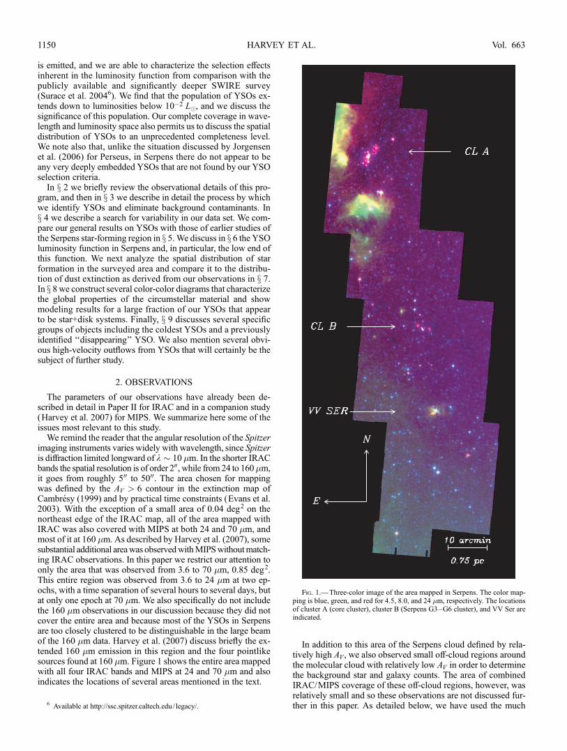
TABLE 2
YSOs in Serpens
ID Name/Position Previous Namea3.6 �m
(mJy)
4.5 �m
(mJy)
5.8 �m
(mJy)
8.0 �m
(mJy)
24.0 �m
(mJy)
70.0 �m
(mJy)
1........... SSTc2d J18275381�0002333 . . . 25.5 � 1.2 20.2 � 1.0 15.6 � 0.7 13.9 � 0.7 22.7 � 2.1 . . .
2b ......... SSTc2d J18280503+0006593 . . . 783 � 55 426 � 29 358 � 18 218 � 14 76.4 � 7.1 . . .
3........... SSTc2d J18280845�0001064 . . . 140 � 7 108 � 8 129 � 6 122 � 8 161 � 14 314 � 36
4b ......... SSTc2d J18281100�0001393 . . . 104 � 5 63.4 � 3.2 54.6 � 2.6 35.4 � 1.9 9.51 � 0.90 . . .
5........... SSTc2d J18281350�0002491 CDF 88-2 105 � 5 88.1 � 4.7 77.5 � 3.7 94.3 � 5.0 254 � 23 382 � 43
6........... SSTc2d J18281501�0002588 . . . 33.3 � 1.6 45.6 � 2.3 61.5 � 3.1 96.3 � 5.8 225 � 20 320 � 41
7........... SSTc2d J18281519�0001405 . . . 7.18 � 0.35 6.18 � 0.30 5.15 � 0.25 5.01 � 0.26 8.00 � 0.77 . . .
8........... SSTc2d J18281525�0002432 CoKu Ser-G1 174 � 9 177 � 9 180 � 11 191 � 11 1200 � 25 1670 � 169
9........... SSTc2d J18281628�0003161 . . . 53.1 � 2.7 48.4 � 2.4 45.4 � 2.1 46.2 � 2.5 74.7 � 6.9 129 � 24
10......... SSTc2d J18281852�0003329 . . . 3.38 � 0.17 3.14 � 0.15 3.13 � 0.16 2.99 � 0.15 2.96 � 0.36 . . .
Notes.—Table 2 is published in its entirety in the electronic edition of the Astrophysical Journal. A portion is shown here for guidance regarding its form and content.a Source names from SIMBAD, including numbers from the following catalogs: EC: Eiroa & Casali (1992); D: Djupvik et al. (2006); K: Kaas et al. (2004).b May be an AGB star, based on Av derived from optical spectrum.
HARVEY ET AL.1154 Vol. 663

order 1� 1 of these are likely to be galaxies. On the other hand,as we discuss in x 6, some of the faint red objects in Figure 3(below the dot-dashed line) may also be young substellar ob-jects. For example, we note the case of the young brown dwarfBD-Ser 1 found by Lodieu et al. (2002) that was not selected byour criteria because of its relative faintness. Of these 235, 198were detected in at least the H and Ks bands of 2MASS at betterthan 7 �. The number of YSOs in each of the four classes of thesystem suggested by Lada (1987) and extended by Greene et al.(1994) is 39 Class I, 25 ‘‘flat,’’ 132 Class II, and 39 Class III,using the flux densities available between 1 and 24 �m. Becausewe require some infrared excess to be identified as a YSO, theClass III candidates were necessarily selected by some measur-able excess typically at the longer wavelengths, 8 or 24 �m. Anobvious corollary is that objects identified as young on the basisof other indicators (e.g., X-ray emission, lithium abundance) butwithout excesses in the range of 1Y24 �m are not selected withour criteria.
3.3. YSOs Selected by MIPS
Harvey et al. (2007) found 250 YSO candidates in the entirearea mapped by MIPS at 24 �m in Serpens, an area of 1.8 deg2;51 of these are outside the IRAC/MIPS overlap area and arelisted in Table 3. We can make a comparison of those statisticswith the YSO counts here in two ways. First, in the area coveredby both IRAC andMIPS-24 there are 197 objects that satisfy thecriteria of Harvey et al. (2007), i.e., Ks < 14, Ks � ½24� > 2,½24�< 10, and 24 �m S/N � 5. Of these, 184 satisfy our more
restrictive criteria in this study based on the combination of2MASS, IRAC, and MIPS data, or 93%. We would classify theother 13 as likely background galaxies. Secondly, of the 235 YSOsfound in this study, 200 have sufficient data to be classifiableby the ‘‘MIPS-only’’ criteria above, but only 167 or 84% actu-ally meet the MIPS-only YSO criteria. In other words, 33 ob-jects have been classified as high-quality YSOs in this paper intheMIPS/IRACoverlap region that did notmeet the criteria basedonly onMIPS and 2MASS data. If these ratios can be extrapolatedto the larger area covered only by MIPS, then we would expectHarvey et al. (2007) to have missed 16% (eight or nine) of theYSOs but to have included 7% (three or four) that would notmeet our combined IRAC/MIPS criteria. With these correctionswe might have expected to find 235þ 56 ¼ 291 YSOs in theentire 1.8 deg2 area covered by MIPS if we had matching IRACobservations. Finally, in light of our earlier discussion of AGBcontaminants, it is possible that six to nine of these YSOs wouldactually be found to be background AGB stars.
4. SEARCH FOR VARIABILITY
The fact that our data were taken in two epochs separated by6 hr or more gives us the opportunity to search for variability overthat timescale. Rebull et al. (2007) and Harvey et al. (2007) haveperformed similar tests for variability of the 24 �m emissionfrom sources in the c2d observations of Perseus and Serpens andfound no reliable evidence for variability at that wavelength.There is, however, substantial evidence for short-term variabilityin the near-infrared for YSOs. We therefore performed a similar
Fig. 5.—Left: Image of the entire mapped area of Serpens at 8.0 �mwith the positions of YSOs plotted with circles and likely extragalactic background contaminantswith asterisks.Middle: Same image with YSOs of luminosity L < 2 ; 10�2 L� plotted with squares and higher luminosity YSOs plotted with circles. Right: Contours ofvisual extinction Av at levels of 5, 10, 20, and 30mag as derived from fitting the energy distributions of sources that were well fitted as reddened stellar photospheres in ourdata set.
SPITZER c2d SURVEY. IX. 1155No. 2, 2007

investigation in the two shortest IRAC bands, 3.6 and 4.5 �m.No clear evidence was found at the level of �25% for anysources in the field over the 6 hr timescale of our multiepochobservations.
5. COMPARISON WITH PREVIOUS STUDIESOF SERPENS
We have cross-correlated our source catalog with those fromprevious studies of Serpens that searched for YSOs. We chosethree studies that covered much of cluster A at near-IR, ISO, and
X-ray wavelengths (Eiroa & Casali 1992; Kaas et al. 2004;Preibisch 2003) and one recent ISO study of cluster B (Djupviket al. 2006). Table 4 lists the sources from each of these previousstudies and the best-matching Spitzer source from our completecatalog. In brief, we find good matches for essentially all the pre-vious IR-selected YSOs that had S/N > 4 in the earlier studiesand that were included in our mapped area. In detail, however,a number of YSO candidates from the earlier studies were notclassified as YSOs in our study. The reasons for this are differentfor the various catalogs. From the X-ray catalog of Preibisch
TABLE 3
YSO Candidates in Serpens without Four-Band IRAC Observations
ID Name/Position Previous Name
3.6 �m
(mJy)
4.5 �m
(mJy)
5.8 �m
(mJy)
8.0 �m
(mJy)
24.0 �m
(mJy)
70.0 �m
(mJy)
236......... SSTc2d J18273421+0040260 . . . . . . . . . . . . . . . 17.8 � 1.7 . . .
237......... SSTc2d J18274024+0035221 . . . . . . . . . . . . . . . 1.36 � 0.25 . . .
238......... SSTc2d J18274264+0020389 . . . . . . . . . . . . . . . 42.0 � 3.9 . . .239......... SSTc2d J18274399+0025135 IRAC 18251+0023 . . . . . . . . . . . . 5430 � 509 655 � 68
240......... SSTc2d J18274484+0052436 . . . . . . . . . . . . . . . 1.49 � 0.27 . . .
241......... SSTc2d J18274506+0006110 IRAS 18251+0004 1730 � 93 . . . 965 � 47 . . . 173 � 16 . . .242......... SSTc2d J18275926+0056012 . . . . . . . . . . . . . . . 40.7 � 3.9 . . .
243......... SSTc2d J18280449+0049498 . . . . . . . . . . . . . . . 15.2 � 1.4 . . .
244......... SSTc2d J18281904+0101333 IRAS 18257+0059 . . . . . . . . . . . . 112 � 10 . . .
245......... SSTc2d J18282591�0032587 IRAS 18258�0034 . . . . . . . . . . . . 279 � 43 . . .246......... SSTc2d J18283708+0149440 . . . . . . . . . . . . . . . 57.3 � 5.3 . . .
247......... SSTc2d J18283939+0106157 IRAS 18261+0104 . . . . . . . . . . . . 356 � 33 . . .
248......... SSTc2d J18284039+0106144 IRAS 18261+0104 . . . . . . . . . . . . 160 � 14 . . .
249......... SSTc2d J18285056+0101121 . . . 4.43 � 0.22 . . . 3.08 � 0.16 . . . 1.93 � 0.31 . . .250......... SSTc2d J18285486+0108548 IRAS 18264+0106 . . . . . . . . . . . . 329 � 30 . . .
251......... SSTc2d J18295035+0008472 . . . . . . 322 � 26 . . . 258 � 14 89.4 � 8.3 . . .
252......... SSTc2d J18295096�0033057 . . . . . . 299 � 20 . . . 146 � 7 50.8 � 4.7 . . .
253......... SSTc2d J18295439+0002476 . . . . . . . . . . . . . . . 77.5 � 7.2 . . .254......... SSTc2d J18300035+0011201 . . . . . . 96.0 � 6.5 . . . 60.7 � 3.3 19.5 � 1.8 . . .
255......... SSTc2d J18300130+0159309 . . . . . . . . . . . . . . . 1.14 � 0.22 . . .
256......... SSTc2d J18300155+0037339 . . . . . . 3.72 � 0.20 . . . 1.94 � 0.11 1.22 � 0.20 . . .257......... SSTc2d J18300181�0037039 IRAS 18275�0039 . . . . . . . . . . . . 29.9 � 2.8 . . .
258......... SSTc2d J18300237+0040549 . . . . . . 4.56 � 0.22 . . . 4.52 � 0.22 3.45 � 0.38 . . .
259......... SSTc2d J18300403+0034240 . . . . . . . . . . . . . . . 217 � 20 798 � 77
260......... SSTc2d J18300528+0036467 . . . . . . . . . . . . . . . 1.93 � 0.25 . . .261......... SSTc2d J18300569+0039318 . . . . . . 19.6 � 1.0 . . . 17.9 � 0.9 34.6 � 3.2 76.2 � 19.5
262......... SSTc2d J18300615+0042339 GSC 00446�00153 . . . 1040 � 58 . . . 1180 � 62 3020 � 283 3920 � 370
263......... SSTc2d J18301017+0039290 . . . . . . 7.50 � 0.37 . . . 8.12 � 0.39 12.2 � 1.1 . . .
264......... SSTc2d J18301188+0036118 . . . . . . . . . . . . . . . 10.8 � 1.0 . . .265......... SSTc2d J18301547+0028278 . . . . . . . . . . . . . . . 2.76 � 0.40 . . .
266......... SSTc2d J18301771+0036115 IRAS 18277+0034 . . . . . . . . . . . . 946 � 87 . . .
267......... SSTc2d J18301831+0021589 IRAS 18277+0019 . . . . . . . . . . . . 320 � 29 . . .268......... SSTc2d J18301943+0055171 . . . . . . 1.64 � 0.08 . . . 0.72 � 0.06 1.63 � 0.26 . . .
269......... SSTc2d J18301948+0037211 . . . . . . . . . . . . . . . 377 � 34 . . .
270......... SSTc2d J18301981+0040273 . . . . . . . . . . . . . . . 2.16 � 0.31 . . .
271......... SSTc2d J18301983+0002536 . . . . . . . . . . . . . . . 122 � 11 . . .272......... SSTc2d J18301991+0041532 . . . . . . . . . . . . . . . 27.2 � 2.5 . . .
273......... SSTc2d J18302200+0043377 . . . . . . . . . . . . . . . 118 � 10 120 � 18
274......... SSTc2d J18302248+0033169 . . . . . . . . . . . . . . . 9.64 � 0.92 . . .
275......... SSTc2d J18302274+0044382 . . . . . . . . . . . . . . . 15.1 � 1.4 . . .276......... SSTc2d J18302320+0033388 . . . . . . . . . . . . . . . 1.70 � 0.24 . . .
277......... SSTc2d J18302326+0042297 HD 170635 . . . . . . . . . . . . 14.8 � 1.4 . . .
278......... SSTc2d J18302419+0035072 . . . . . . . . . . . . . . . 2.39 � 0.31 . . .279......... SSTc2d J18302892+0037532 . . . . . . . . . . . . . . . 3.06 � 0.35 . . .
280......... SSTc2d J18302984+0035007 . . . . . . . . . . . . . . . 26.0 � 2.4 274 � 32
281......... SSTc2d J18303313+0026437 . . . . . . . . . . . . . . . 87.7 � 8.2 . . .
282......... SSTc2d J18303413+0038011 . . . . . . . . . . . . . . . 11.8 � 1.1 . . .283......... SSTc2d J18303587+0040272 . . . . . . . . . . . . . . . 130 � 12 . . .
284......... SSTc2d J18303595+0040385 . . . . . . . . . . . . . . . 71.7 � 6.7 136 � 23
285......... SSTc2d J18303898+0034530 . . . . . . . . . . . . . . . 20.1 � 1.9 . . .
286......... SSTc2d J18304881+0038000 . . . . . . . . . . . . . . . 98.8 � 9.1 . . .
HARVEY ET AL.1156 Vol. 663

(2003) in cluster A, we only identified 17 of the 45 X-ray sourcesas YSOs on the basis of their infrared excesses. The X-raysources that were not identified as YSOs included both manyobjects that were well fitted as reddened stellar photospheres(21 sources) and objects with some likely infrared excess but toolittle to fit our criteria aimed at eliminating extragalactic inter-lopers. The situation with the infrared catalogs is somewhat dif-ferent. Examining our nonmatches from the ground-based studyof Eiroa & Casali (1992), we find that a large fraction of theirYSOs are classified as such by our criteria, but not all. From theISO surveys (Kaas et al. 2004; Djupvik et al. 2006) we typicallyidentify �50%Y60% as YSOs. The ones that we do not classifyas such are typically those with low S/N in the ISO observationsor where the amount of infrared excess was not large enough tosatisfy our test of whether the object could not be fitted as anextincted stellar photosphere as described by Evans et al. (2007).
6. LUMINOSITIES
6.1. The YSO Luminosity Function in Serpens
One of the most important physical parameters for any star isits mass. For preYmain-sequence stars this is problematic be-cause the determination of mass depends on the placement of thestar on an H-R diagram and the use of model evolutionary tracksfor which there is significant uncertainty at the level of at leasta factor of 1.5Y2 in the literature (Hillenbrand & White 2004;Stassun et al. 2004). For young stars in a cluster, a poor but stilluseful proxy for mass is the stellar luminosity since it is possiblethat most of the stars have formed more or less simultaneously.With all these caveats in mind, we display in Figure 6 the histo-gram of total luminosities for the 235 YSOs found in Serpens inour survey with the assumed distance of 260 pc. We remind thereader that these objects were selected specifically on the basisof infrared excess emission, so this list is limited to YSOs thatshow substantial IR excess at least somewhere in the range of3.5Y70 �m. For example, as we discussed in x 5, a comparisonof our list of YSOs with the list of X-ray sources in cluster A(Preibisch 2003) showed that more than half the X-ray sourceswere not classified as YSOs by our infrared excess criteria. Insome sense then, it is likely that the IR-selected and X-rayYselected samples are complementary in selecting less evolvedand more evolved samples of YSOs, respectively. The luminos-ity function of our IR excessYdefinedYSOsample peaks at roughly2 ; 10�2 L� and drops off steeply below 10�2 L�. This is inter-estingly equal to the luminosity of objects at the hydrogen-burning limit of 0.075M� in the models of Baraffe et al. (2002)
for objects with ages of�2Myr, a common estimate for the ageof the Serpens star-forming event (Kaas et al. 2004; Djupviket al. 2006). Of course, an important question to ask is to whatextent this luminosity distribution in Figure 6 is influenced byselection effects.
We can estimate the selection effects in our sample from thestatistics in the SWIRE samples discussed above. The complete-ness limits of the full catalog are nearly 2 mag fainter than thetrimmed version, so we assume for simplicity that the full catalogis 100% complete down to the faintest magnitudes of interest forthis test in the c2d Serpens data set. Figure 7 shows the numbercounts as a function of ‘‘luminosity’’ (all sources assumed to beat 260 pc) for three versions of our c2d-processed SWIRE cat-alog: (1) the full-depth catalog, (2) the catalog cut off with c2dsensitivity limits but without added extinction, and (3) the cat-alog corrected for both c2d sensitivity levels and extinction in theSerpens cloud. The ratio of the second to the first version servesas a good proxy for a completeness function since it includes the
TABLE 4
Matching Spitzer Sources/Fluxes for Previously Identified IR Sources in Serpens
Sourcea Spitzer Source
3.6 �m
(mJy)
4.5 �m
(mJy)
5.8 �m
(mJy)
8.0 �m
(mJy)
24 �m
(mJy)
70 �m
(mJy)
D002................. SSTc2d J18282432+0034545 62.4 � 4.2 46.1 � 3.0 41.1 � 2.5 32.5 � 2.0 13.9 � 1.3 . . .
D001................. SSTc2d J18282442+0026509 105 � 9 95.6 � 7.8 97.9 � 6.5 65.0 � 4.2 13.9 � 1.3 . . .
D003................. SSTc2d J18282649+0031421 38.1 � 2.7 25.8 � 1.7 20.1 � 1.2 12.2 � 0.8 1.26 � 0.28 . . .D004................. SSTc2d J18282783+0028390 6.72 � 0.45 4.47 � 0.29 3.44 � 0.21 2.27 � 0.14 <1.53 . . .
D005................. SSTc2d J18282792+0029288 5.12 � 0.32 3.56 � 0.25 2.76 � 0.16 1.79 � 0.12 <1.45 . . .
D006................. SSTc2d J18282864+0024120 5.68 � 0.38 3.71 � 0.25 3.27 � 0.20 1.92 � 0.12 <1.44 . . .D007................. SSTc2d J18282905+0027561 9.80 � 0.57 8.51 � 0.47 7.03 � 0.38 5.46 � 0.30 43.4 � 4.0 . . .
D008................. SSTc2d J18282912+0034193 193 � 13 93.2 � 6.4 86.6 � 4.5 49.3 � 2.9 5.99 � 0.58 . . .
D010................. SSTc2d J18283208+0025036 11.2 � 0.6 6.47 � 0.38 5.42 � 0.27 3.15 � 0.20 <1.25 . . .
D009................. SSTc2d J18283221+0035361 33.6 � 2.0 20.6 � 1.1 16.1 � 0.9 9.61 � 0.49 0.99 � 0.23 . . .
Notes.—Table 4 is published in its entirety in the electronic edition of theAstrophysical Journal. A portion is shown here for guidance regarding its form and content.a Source numbers from the following catalogs: EC: Eiroa & Casali (1992); D: Djupvik et al. (2006); P: Preibisch (2003); K: Kaas et al. (2004).
Fig. 6.—Luminosity function for Serpens YSOs (solid histogram) and es-timate of correction for completeness effects (dot-dashed histogram).
SPITZER c2d SURVEY. IX. 1157No. 2, 2007

effects of c2d sensitivity only. The bottom panel of Figure 7 thenshows this ratio as our estimate of the completeness function atthe range of luminosities of Serpens YSOs observed in Figure 6.In Figure 6, then, we also indicate how the YSO luminosity func-tion might be adjusted to account for this estimate of our sur-vey completeness (with an assumed completeness of 100% at thebright end). Although substantial adjustments must be made tothe number counts at fainter luminosities, the general conclusionremains intact that the luminosity function peaks around a fewtimes 10�2 L� and drops to both lower and higher luminosities.Interestingly, if our completeness estimates are valid, there maystill be a substantial population of IR excess sources down toluminosities of 10�3 L� as was already suggested in Paper II. Forexample, as noted earlier in x 3.2, the young brown dwarf foundby Lodieu et al. (2002) was not selected as a YSO with our cri-teria because it was faint enough that its colors placed it into thecolor and magnitude ranges where extragalactic objects begin tobe prominent.
6.2. The Lowest Luminosity Sources
There are 37 YSOs with total luminosities (1Y70 �m) lessthan 2 ; 10�2 L�, without any correction for selection effects ineither our observations or our selection criteria. Figure 5 presentedin x 3.2 shows the spatial distribution of the low- (L < 2 ;10�2 L�) and ‘‘high’’-luminosity (L > 2 ; 10�2 L�) YSOs inSerpens. There does not appear to be any significant differencebetween these two distributions. Likewise, Figure 8 shows the
distribution of spectral slopes, �, for the low-luminosity sam-ple relative to two higher luminosity samples, and Table 5 liststhe average and standard deviation for the spectral slopes forthree luminosity samples. Again, there is no obvious differencein the distributions within the statistical uncertainties of thesamples (see also discussion in x 8.1). These two facts suggestthat the mechanisms and timing of formation of these two lu-minosity groups may not be very different. Finally, Figure 9shows the distribution of extinction for stars nearby each YSO.For this analysis we selected all objects within 8000 of each YSOthat were classified as ‘‘star’’ by the process described earlier.We averaged the fitted extinction values for these stars; the num-ber of stars contributing to the average ranged from 5 to 48. Thisfigure shows that the lower luminosity YSOs have at least asmuch typical extinction as the higher luminosity ones, a fact thatwould be unlikely if they were misclassified background extra-galactic objects.
7. SPATIAL DISTRIBUTION OF STAR FORMATION
We have already noted in x 1 that the Serpens star-formingregion has been identified as one displaying strong evidence ofclustering of the youngest objects. We also showed in Figure 5that the spatial distribution of our high-quality YSO candidateswas highly clustered. A number of authors have attempted to quan-tify the degree of clustering as a function of spatial scale usingthe two-point correlation function (Johnstone et al. 2000; Enoch
Fig. 7.—Top: Number counts for the full SWIRE catalog as processedthrough the c2d pipeline for objects detected in all four IRAC bands vs. those forthe ‘‘trimmed’’ version of the catalog with completeness limits for each individ-ual band comparable to those for c2d. Bottom: Ratio of the two number counts,i.e., completeness factor.
Fig. 8.—Histogram of distribution of spectral slopes, ‘‘alpha,’’ for three lu-minosity ‘‘classes’’ of YSOs.
TABLE 5
Average /Standard Deviation of Spectral Slope �versus Luminosity of YSOs
Luminosity Range Average � ��
<0.02 L�.......................... �0.73 1.47
0.02Y1.0 L� ..................... �0.70 1.04
>1.0 L� ............................ �0.60 0.74
HARVEY ET AL.1158 Vol. 663

et al. 2006a; Simon 1997; Gomez&Lada 1998; Bate et al.1998).Typical results have found a steep slope, � / d�2, on small spa-tial scales, implying a rapid decrease in clustering on scales outto �10,000 AU, and a substantially shallower slope, � / d�0:5,beyond that (Simon 1997; Gomez & Lada 1998). Figure 10shows the two-point correlation function,W, for the YSOs in ourSerpens catalog and the sample of objects classified as extra-galactic background sources. The Serpens samples are dividedinto two groups: those with spectral slopes, �, that place them inthe Class I or ‘‘flat’’ categories of Greene et al. (1994), and thosewhose slopes imply Class II or III. Although our range of goodsampling only extends down to�1000 AU, equivalent to 400, ourdata suggest that the slope for separations under 104 AU is oforder 0.5 and drops steeply for the more embedded and likelyyoungest Class I and flat spectral energy distribution (SED)objects beyond 104 AU. The nominally more evolved objects inClasses II and III exhibit a lower level of clustering and moreuniform slope in the two-point correlation function. These re-sults are consistent with the appearance of the source distribu-tions as shown, for example, in Figure 13 of Paper II. As shownin Figure 10, the slope and magnitude of the correlation for oursample of background extragalactic objects are consistent withthose found by, for example, Maddox et al. (1990) for a brightsample of galaxies.
The total surface density of YSOs in a cluster is an indicator ofthe richness of star formation in the cluster. Allen et al. (2007)have computed surface densities for YSOs identified by infraredexcess in a sample of 10 young clusters. They find typical peaksurface densities of 500Y1000 pc�2 and average values of or-der 100Y200 pc�2. The peak surface density in cluster A of ourYSOs identified by IR excess is comparable to these, of order103 pc�2, and a factor of about 2 less in cluster B. The averagevalues are about a factor of 4 less than the peak in both clusters.In particular, if we define the cluster edges by the Av ¼ 20 con-tour for comparison with other c2d clusters, we obtain the values
Fig. 9.—Histogram of distribution of average extinction for stars within8000 of each YSO for ‘‘high’’- and ‘‘low’’-luminosity YSOs (above or below2 ; 10�2 L�).
Fig. 10.—Left: Two-point correlation function, W, for Serpens. The dotted histogram is for sources identified as Class I and flat SED objects, i.e., � � �0:3. Thesolid histogram is for the Class II / III objects, i.e., � < �0:3. The dashed lines show several possible power-law slopes for the portions of the YSO curves. Right: Thedashed histogram is for the objects classified as likely background galaxies with S/N > 7 in all four IRAC bands. The dot-dashed line shows the slope and amplitudefound byMaddox et al. (1990) for the bright end of the extragalactic population, which is a quite good fit to our estimate of the background contamination in our sample.
SPITZER c2d SURVEY. IX. 1159No. 2, 2007

in Table 6 for the number of stars per solid angle and per squareparsec. We have compared the values for clusters A and B withthose for the rest of the cloud and for the total cloud surveyed.The surface densities of YSOs are 10Y20 times higher in theclusters than in the rest of the cloud. As shown by Allen et al.(2007), cluster A in Serpens is particularly striking in terms ofthe contrast between the peak surface density and how quickly,within 1 pc, the density drops to very low values, around a fewpc�2. In terms of volume density, however, even cluster A has asubstantially lower volume density of star formation than suchrich clusters as the Trapezium (5000 pc�3) orMonR2 (9000 pc�3;Elmegreen et al. 2000).
Figure 5 also shows the spatial distribution of visual extinctionin the cloud as derived from our data. These extinction valueswere derived from the combination of 2MASS and Spitzer datafor sources that were well fitted as reddened stellar photospheresas described in detail by Evans et al. (2007). As already noted inour previous studies of the IRAC data alone (Harvey et al. 2006)and the MIPS data alone (Harvey et al. 2007), there is clearly astriking correspondence between the areas of high extinctionand the densest clusters of YSOs, particularly those containingClass I and flat sources.
8. DISK PROPERTIES
The properties of the circumstellar dust surrounding youngstars can be estimated from the overall energy distributions of theobjects in a variety of ways. These properties include the overallamount of dust, the density distribution as a function of radialdistance from the central star, the morphology of the circumstel-lar disks that probably represent the configuration of many ofthese circumstellar distributions, and, to some extent, the degreeof evolution of the dust from typical interstellar dust to larger andmore chemically evolved grains likely to represent some stagein the formation of planetary systems. We discuss several ap-proaches to classifying the dust emission in this section, begin-ning with the use of infrared colors.
8.1. Color-Color Diagrams
Numerous authors have shown how combinations of colors inthe infrared can provide significant diagnostic information on theconfiguration and total amount of circumstellar material aroundyoung stars. Whitney et al. (2003) modeled a wide range of diskand envelope configurations and computed their appearance in anumber of infrared color-color and color-magnitude diagramsparticularly relevant to Spitzer’s wavelength range. Similarly,Allen et al. (2004) have published IRAC color-color diagrams foranother set of models of objects with circumstellar disks and/orenvelopes. Recently, Robitaille et al. (2006) have computed a verylarge grid of models to extend the predictions from those ofWhitney et al. (2003) to a much larger parameter space. Obser-vationally, Lada et al. (2006) have used IRAC and MIPS colorsfrom Spitzer observations to classify the optical thickness ofdisks around preYmain-sequence stars in IC 348, using the terms
‘‘anemic disks’’ and ‘‘thick disks’’ to point to objects roughly inthe Class III and Class II portions of the ubiquitous ‘‘Classsystem’’ (Lada 1987; Greene et al. 1994).Figure 11 shows three color-color diagrams and one color-
magnitude diagram for the 235 Serpens YSOs compared to thedensity of models from Robitaille et al. (2006) for a model clus-ter at the distance of Serpens with brightnesses limited to thoseappropriate for our sensitivity levels. For two of the diagrams thefigure also indicates the approximate areas where most of themodels fall for the three physical stages, I, II, and III, describedby Robitaille et al. (2006) that roughly correspond to the obser-vational ‘‘Classes’’ I+flat, II, and III. These diagrams display,first of all, that YSOs come in a wide range of colors and bright-nesses; large areas of all the diagrams are occupied. In a generalway we find objects located in these diagrams where the modelsof Whitney et al. (2003), Allen et al. (2004), and Robitaille et al.(2006) would predict for preYmain-sequence stars with a rangeof evolutionary states, as well as general agreement with thelocations of young objects found in IC 348 by Lada et al. (2006).For example, consistent with our finding in Paper II that the bulkof the YSOs are Class II objects, we see a strong concentrationin the area around ½5:8� � ½8:0� ¼ 0:8, ½3:6� � ½4:5� ¼ 0:5, whereboth Allen et al. (2004) and Whitney et al. (2003) predict suchsources should be located. In addition, there is structure in the[8.0] versus ½3:6� � ½8:0� color-magnitude diagram for the dis-tribution of Serpens YSOs that is also evident in the density ofmodels of Robitaille et al. (2006). There are, however, someinteresting differences. The ‘‘stage II’’ area from Robitaille et al.(2006) includes a smaller fraction of our nominal Class II objectsthan might be expected. There is also a larger number of very redobjects in several of the diagrams than is predicted by the densityof models in those areas, considering that the faintest gray levelscorrespond to a probability equal to 10�4 of the maximum prob-ability. Some of this may be due to effects of reddening, but itsuggests that the models may also need some refinement, despitetheir rough agreement with the distribution of observed colors.These data can also be examined to see if there is any correla-
tion between luminosity and infrared excess, e.g., the [8.0] versus½3:6� � ½8:0� color-magnitude diagram. For example, if higherluminosity young objects had higher levels of multiplicity (e.g.,Lada 2006), then it is possible that thiswould bemanifested in lessmassive disks with perhaps large inner holes. Figure 11 shows nosuch correlation; in fact, if anything there appears to be a lack ofrelatively blue colors for the brightest objects. Figure 8, whichdisplays the distribution of spectral slopes, and the accompa-nying Table 5 also show no measurable effect within the scatterfor a dependence of spectral slope on luminosity.
8.2. Spectral Energy Distribution Modeling
In order to go beyond the general conclusions possible fromcolor-color and color-magnitude plots, we havemodeled the largefraction of our sources for which enough data are available tocharacterize them as likely star-plus-disk objects. For this analysis
TABLE 6
Numbers, Densities, Star Formation Rates
Region Area
N(YSOs)
(pc2)
N/�
(deg�2)
N/Area
(pc�2)
N/Volume
(pc�3)
SFR
(M� Myr�1)
SFR/Area
(M� Myr�1 pc�2)
Cluster A.................... 0.20 44 4580 222 500 11 56
Cluster B .................... 0.14 17 2450 119 315 4.3 30
Rest of cloud.............. 17.2 174 209 10.1 2.5 44 2.5
All of cloud................ 17.5 235 276 13.4 3.2 59 3.4
HARVEY ET AL.1160 Vol. 663

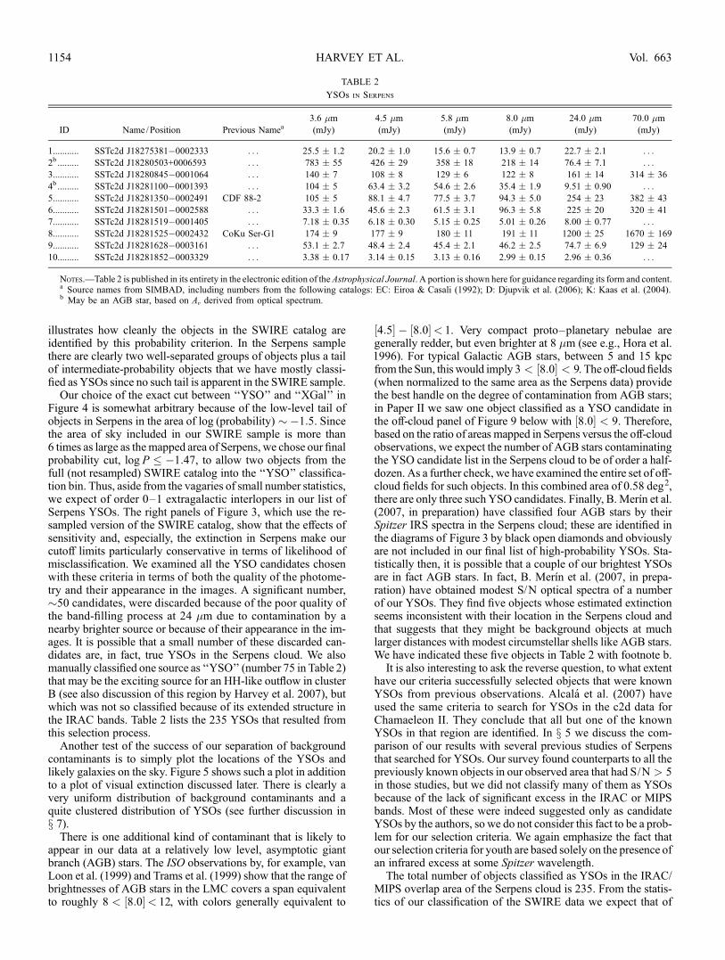
we have selected all Class II and Class III YSOs.We expect theseobjects to have a reddened photosphere plus an infrared excesscoming from the circumstellar material, most likely in a diskconfiguration. For completeness we show, without modeling, theSEDs of the remaining YSOs. Figures 12Y20 show the SEDs ofall Class I, flat, Class II, and Class III sources. The open circlesshow the observed fluxes and generally include 2MASS J, H,and K fluxes followed by the four IRAC fluxes at 3.6, 4.5, 5.8,and 8.0 �m and by the MIPS fluxes at 24 and 70 �mwhen avail-able. For the Class II and III sources, we characterize the emis-sion from the disk by comparing the energy distribution with thatof a low-mass star. For this, we have computed the extinctionfrom the J � K colors assuming a K7 underlying star, and thenwe have dereddened the observed fluxes with the interstellarextinction law of Weingartner & Draine (2001) with Rv ¼ 5:5 tofit the dereddened SEDs to aNEXTGEN (Hauschildt et al. 1999)model of a K7 stellar photosphere. In the plots, the filled circlesshow the dereddened fluxes and the gray line shows the photo-spheric emission from the star. Each SED is labeled with theidentification number in Table 2. The parameters of the modelfits are listed in Tables 7 and 8.
Two main assumptions are used in this approach. The first isthat the star is a low-mass star; this is reasonable given the factthat the luminosity function discussed earlier peaks at L � few ;10�2 L�. In addition, J. M. Oliveira et al. (2007, in preparation)have found that 30 of the 39 YSOs they observed out of our sam-ple had spectral types of K or M. The second assumption is that
there is no substantial excess in the near-infrared bands, wherewe consider all flux to be photospheric. This assumption is ob-viously only correct for those stars in the sample without strongongoing disk accretion. Cieza et al. (2005) have demonstratedthat near-IR excesses as short as J band can be seen in someactively accreting T Tauri stars, and they give an observed rangeof J-band excesses of 0.1Y1.0 mag for their sample of sources inTaurus. The effect of this excess on the computed parametersimplies that the stellar luminosities for the Class II objects areupper limits and therefore the disk luminosities are lower lim-its. More specifically, neglecting an excess flux in the J band of1.1 mag in one object would reduce its Ldisk/Lstar ratio by 12%and modify the disk emission SED, diminishing its excessmostly at the shorter wavelengths. That would only happen, how-ever, to the fraction of objects that are strongly accreting. J. M.Oliveira et al. (2007, in preparation) found strong H� emissionindicative of active accretion in only 12 out of 39 Serpens YSOsobserved. We ran a test removing these objects from the finalstatistics, and this did not change the overall picture.
The dashed line in the SED plots is the median SED of T Tauristars in Taurus (Hartmann et al. 2005) normalized to the dered-dened J-band flux of our SEDs. It represents the typical SED ofan optically thick accreting disk around a classical T Tauri star(CTTS) and is shown here to allow a qualitative estimation of thepresence of disk evolution and dust settling. Based on similarityto this median SED, we define as ‘‘T’’ an SED that is identical toit, within the errors, as ‘‘L’’ an SED with lower fluxes at some
Fig. 11.—Color-color and color-magnitude plots of the 235 Serpens YSOs compared with the distributions frommodels of Robitaille et al. (2006). The symbols arefor the three different luminosity groups discussed in the text: L > 1 L� (open diamonds), 0:02 L� < L < 1 L� (gray filled circles), and L < 0:02 L� ( plus signs). Themodel data were those for their model cluster, with a distance of 260 pc for Serpens and with the c2d completeness limits. Also shown are the rough areas fromRobitailleet al. (2006) occupied by mainly stage I, II, and III models.
SPITZER c2d SURVEY. IX. 1161No. 2, 2007
Fig. 12.—SEDs of the Class I sources in the sample. The open circles signal the observed fluxes from J band toMIPS-70 when available. The label gives the index inTable 2.
1162

Fig. 13.—SEDs of the Class I sources in the sample (continued). Symbols as in Fig. 12.
Fig. 14.—SEDs of the flat sources in the sample. Symbols as in Fig. 12.
1163
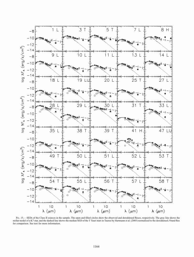
Fig. 15.—SEDs of the Class II sources in the sample. The open and filled circles show the observed and dereddened fluxes, respectively. The gray line shows thestellar model of a K7 star, and the dashed line shows the median SED of the T Tauri stars in Taurus by Hartmann et al. (2005) normalized to the dereddened J-band fluxfor comparison. See text for more information.
1164

Fig. 16.—SEDs of the Class II sources in the sample (continued).
1165
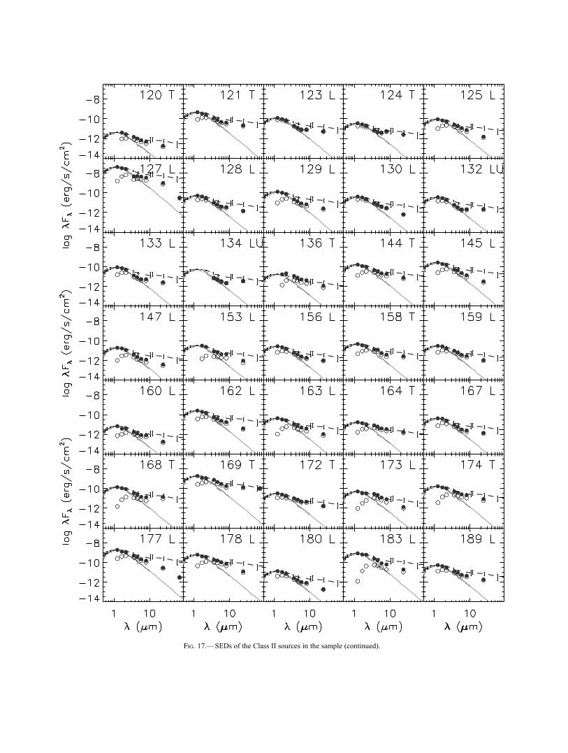
Fig. 17.—SEDs of the Class II sources in the sample (continued).

wavelengths, and as ‘‘H’’ an object with larger fluxes than themedian T Tauri SED. We have labeled the objects with thesecodes and use them to interpret the state of disk evolution. Weinterpret the L-type objects as thin disks that could perhaps resultfrom dust grain growth and settling to the midplane, similar tothe anemic disks in Lada et al. (2006). Objects 3 and 5 are goodexamples of T-type objects, numbers 11 and 18 are L-type stars,and number 8 is an H-type object. Also, we have labeled as‘‘LU’’ objects that have photospheric fluxes up to around 8 �mbut then a sudden jump at longer wavelengths to the levels of a
T Tauri disk. We believe that these objects may have large innerholes in their still optically thick disks; number 19 is one ex-ample of these.
Out of the 171 sources in the sample that are Class II orClass III, 44 (26%) are T type and so equivalent to a CTTS,125 (73%) are L type and so show evidence of some degree of diskevolution, and finally 2 (1%) show larger fluxes than the medianSED of Taurus. The latter category is generally the result of im-perfect fitting to the stellar photosphere due to lack of near-IR dataand will not be considered further.
Fig. 18.—SEDs of the Class II sources in the sample (continued).
SPITZER c2d SURVEY. IX. 1167
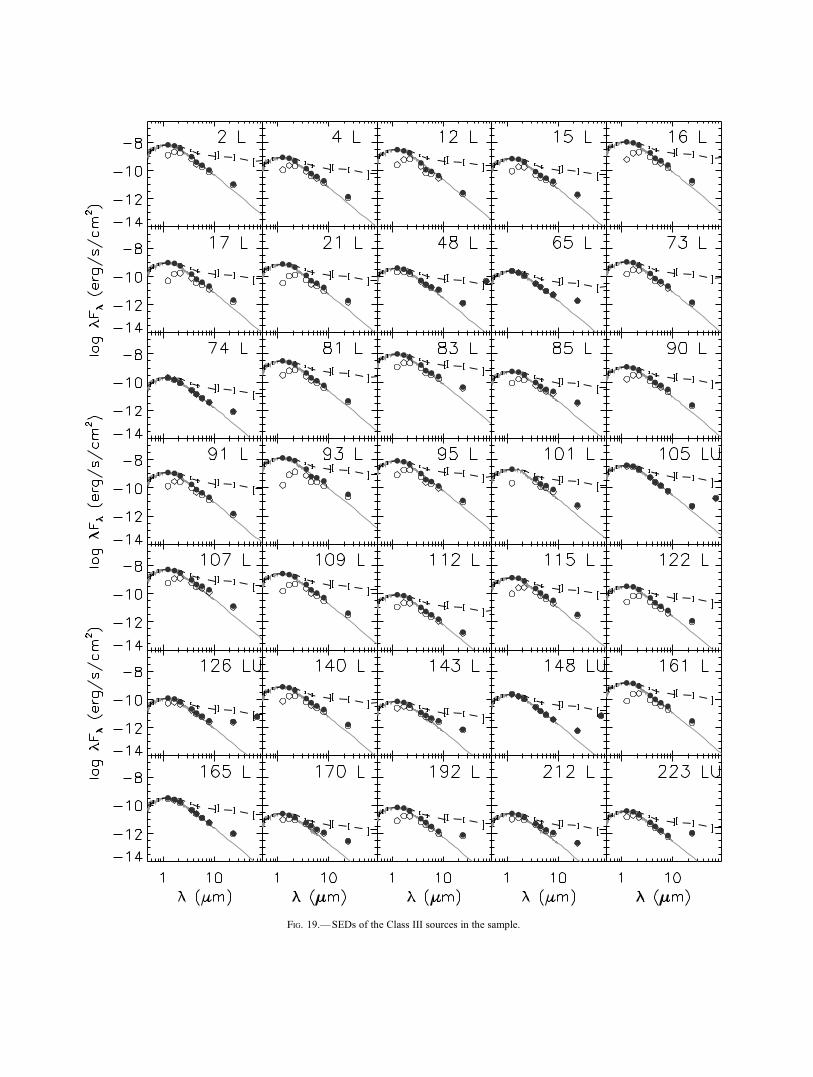
Fig. 19.—SEDs of the Class III sources in the sample.
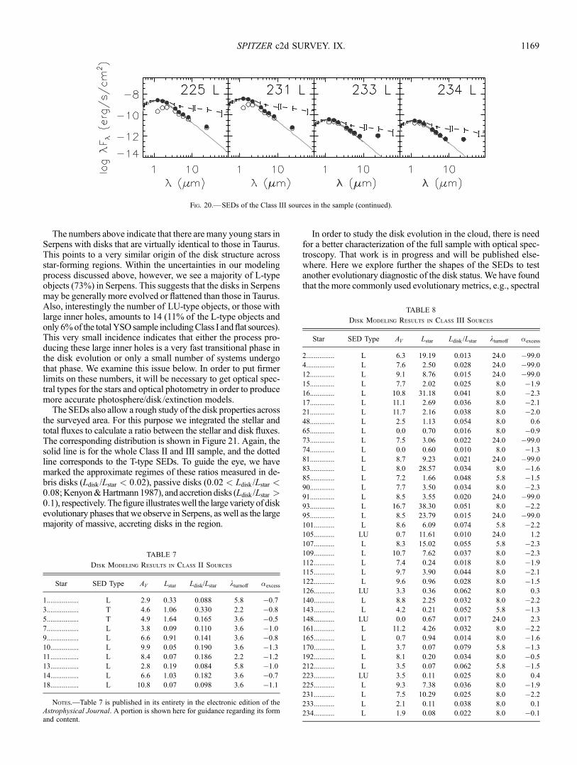
The numbers above indicate that there are many young stars inSerpens with disks that are virtually identical to those in Taurus.This points to a very similar origin of the disk structure acrossstar-forming regions. Within the uncertainties in our modelingprocess discussed above, however, we see a majority of L-typeobjects (73%) in Serpens. This suggests that the disks in Serpensmay be generally more evolved or flattened than those in Taurus.Also, interestingly the number of LU-type objects, or those withlarge inner holes, amounts to 14 (11% of the L-type objects andonly 6%of the totalYSO sample includingClass I and flat sources).This very small incidence indicates that either the process pro-ducing these large inner holes is a very fast transitional phase inthe disk evolution or only a small number of systems undergothat phase. We examine this issue below. In order to put firmerlimits on these numbers, it will be necessary to get optical spec-tral types for the stars and optical photometry in order to producemore accurate photosphere/disk/extinction models.
The SEDs also allow a rough study of the disk properties acrossthe surveyed area. For this purpose we integrated the stellar andtotal fluxes to calculate a ratio between the stellar and disk fluxes.The corresponding distribution is shown in Figure 21. Again, thesolid line is for the whole Class II and III sample, and the dottedline corresponds to the T-type SEDs. To guide the eye, we havemarked the approximate regimes of these ratios measured in de-bris disks (Ldisk /Lstar < 0:02), passive disks (0:02 < Ldisk /Lstar <0:08;Kenyon&Hartmann1987), and accretion disks (Ldisk /Lstar >0:1), respectively. Thefigure illustrateswell the large variety of diskevolutionary phases that we observe in Serpens, as well as the largemajority of massive, accreting disks in the region.
In order to study the disk evolution in the cloud, there is needfor a better characterization of the full sample with optical spec-troscopy. That work is in progress and will be published else-where. Here we explore further the shapes of the SEDs to testanother evolutionary diagnostic of the disk status. We have foundthat the more commonly used evolutionary metrics, e.g., spectral
Fig. 20.—SEDs of the Class III sources in the sample (continued).
TABLE 7
Disk Modeling Results in Class II Sources
Star SED Type AV Lstar Ldisk/Lstar kturnoff �excess
1................. L 2.9 0.33 0.088 5.8 �0.7
3................. T 4.6 1.06 0.330 2.2 �0.8
5................. T 4.9 1.64 0.165 3.6 �0.5
7................. L 3.8 0.09 0.110 3.6 �1.0
9................. L 6.6 0.91 0.141 3.6 �0.8
10............... L 9.9 0.05 0.190 3.6 �1.3
11............... L 8.4 0.07 0.186 2.2 �1.2
13............... L 2.8 0.19 0.084 5.8 �1.0
14............... L 6.6 1.03 0.182 3.6 �0.7
18............... L 10.8 0.07 0.098 3.6 �1.1
Notes.—Table 7 is published in its entirety in the electronic edition of theAstrophysical Journal. A portion is shown here for guidance regarding its formand content.
TABLE 8
Disk Modeling Results in Class III Sources
Star SED Type AV Lstar Ldisk /Lstar kturnoff �excess
2............... L 6.3 19.19 0.013 24.0 �99.0
4............... L 7.6 2.50 0.028 24.0 �99.0
12............. L 9.1 8.76 0.015 24.0 �99.0
15............. L 7.7 2.02 0.025 8.0 �1.9
16............. L 10.8 31.18 0.041 8.0 �2.3
17............. L 11.1 2.69 0.036 8.0 �2.1
21............. L 11.7 2.16 0.038 8.0 �2.0
48............. L 2.5 1.13 0.054 8.0 0.6
65............. L 0.0 0.70 0.016 8.0 �0.9
73............. L 7.5 3.06 0.022 24.0 �99.0
74............. L 0.0 0.60 0.010 8.0 �1.3
81............. L 8.7 9.23 0.021 24.0 �99.0
83............. L 8.0 28.57 0.034 8.0 �1.6
85............. L 7.2 1.66 0.048 5.8 �1.5
90............. L 7.7 3.50 0.034 8.0 �2.3
91............. L 8.5 3.55 0.020 24.0 �99.0
93............. L 16.7 38.30 0.051 8.0 �2.2
95............. L 8.5 23.79 0.015 24.0 �99.0
101........... L 8.6 6.09 0.074 5.8 �2.2
105........... LU 0.7 11.61 0.010 24.0 1.2
107........... L 8.3 15.02 0.055 5.8 �2.3
109........... L 10.7 7.62 0.037 8.0 �2.3
112........... L 7.4 0.24 0.018 8.0 �1.9
115........... L 9.7 3.90 0.044 8.0 �2.1
122........... L 9.6 0.96 0.028 8.0 �1.5
126........... LU 3.3 0.36 0.062 8.0 0.3
140........... L 8.8 2.25 0.032 8.0 �2.2
143........... L 4.2 0.21 0.052 5.8 �1.3
148........... LU 0.0 0.67 0.017 24.0 2.3
161........... L 11.2 4.26 0.032 8.0 �2.2
165........... L 0.7 0.94 0.014 8.0 �1.6
170........... L 3.7 0.07 0.079 5.8 �1.3
192........... L 8.1 0.20 0.034 8.0 �0.5
212........... L 3.5 0.07 0.062 5.8 �1.5
223........... LU 3.5 0.11 0.025 8.0 0.4
225........... L 9.3 7.38 0.036 8.0 �1.9
231........... L 7.5 10.29 0.025 8.0 �2.2
233........... L 2.1 0.11 0.038 8.0 0.1
234........... L 1.9 0.08 0.022 8.0 �0.1
SPITZER c2d SURVEY. IX. 1169

slope �, bolometric temperature Tbol, or the Class system dis-cussed earlier, do not seem to capture the full range of phenom-ena apparent in our distribution of SEDs for YSOs. We thereforeuse �excess and kexcess, two new second-order SED parameterspresented in Cieza et al. (2007) that will be discussed in moredetail in a separate paper. In short, kexcess is the last wavelengthwhere the observed flux is photospheric and �excess is the slopecomputed as d log (kFk)/d log k starting from kexcess. The firstparameter gives us an indication of how close the circumstellarmatter is to the central object, and the latter one a measure of howoptically thick it is. Given the assumptions above for the fittingprocess, our values are upper limits for kexcess and correspond-ingly lower limits for �excess for the Class II sources. We assumegood stellar fits for the Class III sources.
Figure 22 shows both values for a sample of CTTSs fromCieza et al. (2005), weak-lined T Tauri stars (WTTSs) fromCieza et al. (2007), debris disks from Chen et al. (2005), and oursample of YSOs in Serpens. Cieza et al. (2007) found that kexcessis well correlated with evolutionary phase and also, as seen inFigure 22, that � is observed over wider ranges for later evolu-tionary phases. This suggests a large range of possible evolu-tionary paths for circumstellar disks. Objects could evolve to thelower right side of the diagram, which could be interpreted as asign of dust grain growth and settling to the disk midplane; theycould alsomove to the right and up, from creation of a large innerhole in their disks while retaining a massive outer disk, and also,as this diagram shows, all intermediate pathways in betweenboth extremes.
9. SELECTED SOURCES
9.1. The Coldest Objects
Table 9 lists the 15 YSOs that display the coldest energydistributions. These are the objects with a ratio of F70 /F24 > 8.Six of these are in cluster A (the core) and four in cluster B. Twoare in a small grouping about 0.2
�northeast of cluster B, and the
remaining three appear as isolated cold objects, although in areaswith other moderately red objects. All of these except for two ofthe isolated cold objects, IDs 105 and 148, are associated withdense clumps of millimeter emission as seen by Enoch et al.
(2006b). As discussed in the following section, two in cluster Aand one in cluster B are associated with high-velocity outflows.As has been noted already byPadgett et al. (2004) andRebull et al.(2007), it is striking how many of these coldest, most obscuredYSOs are located in compact clusters together with objects thatare substantially more evolved in the nominal system of classes,e.g., Class II and III.
9.2. Outflow Sources
A number of recent Spitzer studies have found that high-velocity shocked outflows from young stars are visible in IRACimages, typically strongest at 4.5 �m (Noreiga-Crespo et al.2004). We have examined our images for such outflows, as wellas for correspondence with the lists of published HH objects inthe region (Ziener & Eisloffel 1999). Table 10 summarizes theresults of this effort. Two strong, obvious jetlike features are seenin cluster A and one in cluster B. In addition, as shown inTable 10,we find small extended features at the positions of most of theknown HH objects in Serpens that were within our covered area.The two ‘‘jets’’ in cluster A appear to originate from two of themost deeply embedded objects in this cluster that are associatedwith the submillimeter sources SMM 1 and SMM 5 (Testi &Sargent 1998). Both of these outflows are aligned roughly in thenorthwest-southeast direction and are visible on both sides of thecentral 24 �m likely exciting sources. In cluster B there is oneobvious jetlike feature extendingmostly south of YSO 75. Thereis also probably faint emission visible 3000 to the north of theembedded source. Harvey et al. (2007) discuss the cluster B jetand several nearby Spitzer sources in more detail. Figures 23 and24 show three-color images of clusters A and B with the colortables chosen to make these jets most visible. In addition to theoptical HH objects in the Serpens clouds, there are a number ofhigh-velocity molecular outflows that have been mapped in clus-ter A (Davis et al. 1999). These maps present a confusing pictureof outflows, and because of the relatively larger beamwidth ofthemillimeter observations and close packing of infrared sourcesin this cluster, it is very difficult to associate the radio outflowsunequivocally with particular Spitzer sources.
Fig. 21.—Distribution of disk-to-star luminosity ratios. The solid and dashedhistograms are for the total sample and T TauriY like sample of SEDs, respectively.Also marked are the typical ranges of Ldisk /Lstar ratios for debris disks, passive ir-radiated disks, and accretion disks. The figure indicates that objects of all threeevolutionary stages are found in Serpens, with a predominance of young accretingT TauriY type stars.
Fig. 22.—Distribution of excess slopes �excess with respect to the wave-length at which the infrared excess begins kturnoff for the sample of WTTSs( filled circles), a sample of CTTSs in Lupus from Cieza et al. (2007), the me-dian SED of CTTSs in Taurus from D’Alessio et al. (1999) in asterisks (markedas D99), and a sample of debris disks from Chen et al. (2005) in diamonds. Theplus signs represent the limits for the Class II objects in Serpens, and the tri-angles the Class III sources. The diagram shows a much larger spread in innerdisk morphologies in the more evolved objects than in the least evolved ones.The Serpens objects follow the previously observed trend.
HARVEY ET AL.1170 Vol. 663

9.3. Other Objects
Horrobin et al. (1997) reported on the disappearance of abright near-infrared source in Serpens from the earlier study ofEC 92. Table 4 shows that we also see no obvious source at theposition of EC 92-81, other than a low-S/N single-band detec-tion of a source moderately distant from the nominal position.Interestingly, however, this area marked in Figure 23 appearsto contain several small knots of emission that may representshocked gas. For example, there are two small knots visible inour 4.5 and 8.0 �m images that have no 3.6 or 24 �m counter-parts (and therefore not classified as YSOs). These two knots, atR:A: ¼ 18h29m56:7s, decl: ¼ þ01�1301900 (J2000.0), are only1200 south of the position of EC 92-81. Therefore, it is possiblethat the original source was a small clump of excited gas that hasmoved or dissipated since the original study of EC 92, and per-haps these Spitzer knots are related to that earlier source in someway.
10. OVERALL RESULTS ON STAR FORMATION
The overall picture of star formation in Serpens is summarizedin Table 6. As noted earlier, the surface density of young stars ismuch higher in clusters A and B than in the rest of the cloud, by
factors of 10Y20. On the other hand, the majority of YSOs (74%)are not in the clusters, but in the rest of the cloud. If we assume amean mass for the stars of 0.5M� and assume that star formationhas been proceeding for 2 Myr, we can estimate the rate at whichthe clusters and the whole cloud are converting mass into stars.These values are also given in Table 6. The Serpens cloud that wehave surveyed is turning nearly 60 M� into stars per Myr. Therates for the clusters are probably underestimates because theyare probably younger than 2 Myr, a typical duration for theClass II SED. Of course, a significant number of the older objectsoutside the clusters may have, in fact, formed in these or earlierclusters. A 1 km s�1 random motion of a YSO relative to itsbirthplace results in 1 pc of movement in 106 yr, or nearly 0.25� atthe distance of Serpens.
The distribution of YSOs over class supports the younger agefor the clusters than for star formation in general in Serpens.Whilethe ratio of the number of Class I and flat-spectrum sources tothe number of Class II and Class III sources is 0.37 for the wholecloud, similar to other clouds surveyed by c2d (N. J. Evans et al.2007, in preparation), the same ratio is 3.0 for cluster A and 1.4for cluster B. These high ratios strongly suggest that cluster Ais too young for most YSOs to have reached the Class II stage. Incontrast, this ratio is 0.14 for the rest of the cloud, outside the
TABLE 9
The Coldest YSOs (F70 /F24 > 8)
ID
(Table 2) Name/Position
3.6 �m
(mJy)
4.5 �m
(mJy)
5.8 �m
(mJy)
8.0 �m
(mJy)
24.0 �m
(mJy)
70.0 �m
(mJy)
40........................ SSTc2d J18285404+0029299 5.81 � 0.50 27.6 � 2.3 44.8 � 2.6 56.4 � 3.2 918 � 85 11100 � 1040
42........................ SSTc2d J18285486+0029525 1.94 � 0.12 10.6 � 0.6 20.4 � 1.1 30.2 � 1.6 765 � 70 7250 � 675
48........................ SSTc2d J18285808+0017244 52.5 � 3.0 36.7 � 2.5 31.2 � 1.7 28.5 � 1.7 9.74 � 0.92 1040 � 101
60........................ SSTc2d J18290211+0031206 1.19 � 0.07 1.62 � 0.09 1.58 � 0.10 1.13 � 0.07 22.1 � 2.0 276 � 29
68........................ SSTc2d J18290675+0030343 3.27 � 0.21 11.7 � 0.7 14.9 � 0.8 20.7 � 1.2 1000 � 105 11400 � 1180
105...................... SSTc2d J18293254�0013233 654 � 39 370 � 19 276 � 13 156 � 8 39.7 � 3.7 429 � 47
135...................... SSTc2d J18294810+0116449 1.96 � 0.10 6.98 � 0.42 12.1 � 0.6 16.7 � 0.8 219 � 21 14900 � 1420
141...................... SSTc2d J18294963+0115219 0.85 � 0.08 2.64 � 0.27 2.32 � 0.28 3.54 � 0.31 1180 � 117 82800 � 7810
146...................... SSTc2d J18295114+0116406 31.1 � 2.6 72.6 � 4.6 141 � 7 208 � 10 992 � 92 8480 � 805
148...................... SSTc2d J18295130+0027479 33.8 � 2.0 22.3 � 1.3 16.2 � 0.9 10.1 � 0.6 4.81 � 0.50 163 � 18
150...................... SSTc2d J18295219+0115478 7.38 � 0.41 33.0 � 2.1 41.3 � 2.2 40.0 � 2.6 1640 � 154 15200 � 1420
154...................... SSTc2d J18295252+0036117 2.49 � 0.14 4.24 � 0.23 5.18 � 0.28 6.55 � 0.36 100 � 9 1910 � 179
166...................... SSTc2d J18295430+0036013 2.39 � 0.25 6.57 � 0.42 7.32 � 0.44 5.80 � 0.31 16.0 � 1.5 1270 � 121
195...................... SSTc2d J18295927+0114016 2.72 � 0.28 5.76 � 0.44 7.78 � 1.16 36.0 � 5.4 109 � 19 12200 � 1160
203...................... SSTc2d J18300070+0113014 0.38 � 0.04 1.23 � 0.10 2.08 � 0.16 3.55 � 0.21 95.8 � 11.4 8640 � 829
TABLE 10
Probable High-Velocity Outflows in Serpens
YSO ID
R.A.
(J2000.0)
Decl.
(J2000.0) Matching Name Comments
18 29 18.8 +01 14 15 HH 106A, B, E
18 29 47.7 +01 25 52 HH 107A
18 30 22.7 +01 16 18 HH 455A
18 30 22.6 +01 16 05 HH 455B, D
18 30 02.6 +01 14 45 HH 459A, B
18 29 38.5 +01 18 26 HH 460A, B, C, D
18 29 56.6 +01 15 37 HH 478A, B
141 18 29 49.6 +01 15 21 SMM 1 Jets to NW and SE
146 18 29 51.2 +01 16 41 SMM 5 Jets to NW and SE
75 18 29 09.0 +00 31 30 . . . Jets to N and S
Note.—Units of right ascension are hours, minutes, and seconds, and units of declination aredegrees, arcminutes, and arcseconds.
SPITZER c2d SURVEY. IX. 1171No. 2, 2007

clusters, which is strongly dominated by Class II and Class IIIobjects.
11. SUMMARY
We have identified a high-confidence set of 235 YSOs inSerpens by a set of criteria based on comparison with data fromthe Spitzer SWIRELegacy program. This is a large enough num-ber that we can draw important statistical conclusions aboutvarious properties of this set. If we assume that the ‘‘Class sys-tem’’ of Lada (1987) and Greene et al. (1994) represents an evo-lutionary sequence, then the relative numbers of YSOs foundin each of the first three classes ( I, flat, and II ) suggest that theClass II phase lasts substantially longer than the combined totalof the Class I and flat phases, based on the overall cloud statistics.The clusters, however, show more YSOs in the Class I and flatphases than in Class II, indicating that they are very young. Themajority of YSOs (mostly Class II ) are outside the clusters andprobably represent a somewhat older epoch of star formation com-pared to the intense star formation now going on in the clusters.The surface density of YSOs in the clusters exceeds that of the restof the cloud by factors of 10Y20 (Table 6).
The luminosity function for the Serpens YSOs is populateddown to luminosities of 3 ; 10�3 L�. It may extend even lower,but our ability to distinguish low-luminosity YSOs is severelyrestricted by the large population of background galaxies at theseflux levels. The lower luminosity YSOs, L < 2 ; 10�2 L�, ex-hibit a similar spatial distribution and SED slope distribution tothose of their higher luminosity counterparts. This is consistentwith the conclusion that they have formed in similar ways.
Support for this work, part of the Spitzer Legacy ScienceProgram, was provided by NASA through contracts 1224608,1230782, and 1230779 issued by the Jet Propulsion Laboratory,California Institute of Technology, under NASA contract 1407.Astrochemistry in Leiden is supported by an NWO Spinozagrant and a NOVA grant. B. M. thanks the Fundacion RamonAreces for financial support. This publication makes use of dataproducts from the Two Micron All Sky Survey, which is a jointproject of the University of Massachusetts and the Infrared Pro-cessing and Analysis Center/California Institute of Technology,funded by NASA and the National Science Foundation. We alsoacknowledge extensive use of the SIMBAD database.
APPENDIX
YSO SELECTION PROCESS
The procedure we use to select YSOs and deselect extragalactic background sources is based on the color-magnitude diagrams shown inFigure 3.Weconstruct ‘‘probability’’ functions for each of the three color-magnitude diagrams based onwhere a source falls relative to the blackdashed lines in each diagram. These three probabilities are multiplied, and then additional adjustments to the probability are made based onseveral additional properties of the source fluxes andwhether or not theywere found to be larger than pointlike in the source extraction process.
In the [4.5] versus ½4:5� � ½8:0� color-magnitude diagram, the probability function is
Pi2i4 ¼ 0:7 1� exp � 1:2þ 0:5 M4:5 � Dð Þ½ �3n o� �
;
where
D ¼
13:05; M4:5 �M8:0 > 1:4;
14:5; 0:5 � M4:5 �M8:0 < 1:4;
12:5; 0:5 � M4:5 �M8:0 < 1:4;
14:5; M4:5 �M8:0 < 0:5
8>>><>>>:
Fig. 23.—Three-color image of the cluster A area of Serpens. The color cod-ing is blue, green, and red for 4.5, 8.0, and 24 �m, respectively. Some of themore obvious objects that are likely to be jets aremarked by arrows. The region ofthe disappearing source 81 of Eiroa & Casali (1992) is circled.
Fig. 24.—Three-color image of the cluster B area of Serpens as for Fig. 23.
HARVEY ET AL.1172 Vol. 663

(for the second value ofD, the object was found to be pointlike in all IRAC bands, and for the third value ofD, the object was found to beextended at 3.6 or 4.5 �m).
In the [24] versus ½8:0� � ½24� color-magnitude diagram, the probability function is
Pi4m1 ¼ exp � M8 �M24 � 3:5ð Þ=1:7½ � 2þ M24 � 9ð Þ=2½ �n o 2
� �;
and Pi4m1 is set to a minimum of 0.1.In the [24] versus ½4:5� � ½8:0� color-magnitude diagram, the probability function is
Pi24m1 ¼ 0:7 1� exp � M4:5 �M8 þ 0:8� 10�M24ð Þ=1:8½ �f gð Þ;
and Pi24m1 is set to a minimum of 0.The combined probability is then
Ptot ¼ Pi2i4Pi4m1Pi24m1:
In addition, the following factors influence modifications to Ptot: Ptot /(K � ½4:5�), Ptot ; 2 for sources that are extended at 3.6 or 4.5 �m,Ptot ¼ 0:1 where ½24�> 10 (i.e., assumed GALc), and Ptot ; 0:1 where F70 > 400 mJy and source detected at 5.8, 8, and 24 �m.
Based on the distribution of Ptot shown in Figure 4, we chose the dividing line between YSOs and extragalactic sources to belog10 Ptot ¼ �1:47.
REFERENCES
Alcala, J., et al. 2007, ApJ, submittedAllen, L. E., et al. 2004, ApJS, 154, 363———. 2007, in Protostars and Planets V, ed. B. Reipurth, D. Jewitt, & K. Keil(Tucson: Univ. Arizona Press), 361
Baraffe, I., Chabrier, G., Allard, F., & Hauschildt, P. H. 2002, A&A, 382, 563Bate, M. R., Clarke, C. J., & McCaughrean, M. J. 1998, MNRAS, 297, 1163Cambresy, L. 1999, A&A, 345, 965Casali, M. M., Eiroa, C., & Duncan, W. D. 1993, A&A, 275, 195Chen, C. H., et al. 2005, ApJ, 634, 1372Cieza, L., et al. 2005, ApJ, 635, 422———. 2007, ApJ, in pressD’Alessio, P., Calvet, N., Hartmann, L., Lizano, S., & Canto, J. 1999, ApJ, 527,893
Davis, C. J., Matthews, H. E., Ray, T. P., Dent, W. R. F., & Richer, J. S. 1999,MNRAS, 309, 141
Djupvik, A. A., Andre, Ph., Bontemps, S., Motte, F., Olofsson, G., Galfalk, M.,& Floren, H.-G. 2006, A&A, 458, 789
Eiroa, C., & Casali, M. M. 1992, A&A, 262, 468Eiroa, C., Djupvik, A. A., & Casali, M. M. 2007, in ASP Conf. Ser., Handbookof Star Forming Regions, ed. B. Reipurth (San Francisco: ASP), in press
Elmegreen, B. G., Efremov, Y., Pudritz, R. E., & Zinnecker, H. 2000, in Proto-stars and Planets IV, ed. V. Mannings, A. P. Boss, & S. S. Russell (Tucson:Univ. Arizona Press), 179
Enoch, M. L., et al. 2006a, ApJ, 638, 293———. 2006b, ApJ, submittedEvans, N. J., II, et al. 2003, PASP, 115, 965———. 2007, Final Delivery of Data from the c2d Legacy Project: IRAC andMIPS (Pasadena: SSC)
Gomez, M., & Lada, C. J. 1998, AJ, 115, 1524Greene, T. P., Wilking, B. A., Andre, P., Young, E. T., & Lada, C. J. 1994, ApJ,434, 614
Hartmann, L., Megeath, S. T., Allen, L., Luhman, K., Calvet, N., D’Alessio, P.,Franco-Hernandez, R., & Fazio, G. 2005, ApJ, 629, 881
Harvey, P. M., Wilking, B. A., & Joy, M. 1984, ApJ, 278, 156Harvey, P. M., et al. 2006, ApJ, 644, 307 (Paper II )———. 2007, ApJ, 663, 1139Hauschildt, P. H., Allard, F., Ferguson, J., Baron, E., & Alexander, D. R. 1999,ApJ, 525, 871
Hillenbrand, L. A., & White, R. J. 2004, ApJ, 604, 741
Hogerheijde, M. R., van Dishoeck, E. F., & Salverda, J. M. 1999, ApJ, 513, 350Hora, J. L., Deutsch, L. K., Hoffmann,W. F., & Fazio, G. G. 1996, AJ, 112, 2064Horrobin, M. J., Casali, M. M., & Eiroa, C. 1997, A&A, 320, L41Hurt, R. L., & Barsony, M. 1996, ApJ, 460, L45Johnstone, D., Wilson, C. D., Moriarty-Schieven, G., Joncas, G., Smith, G.,Gregersen, E., & Fich, M. 2000, ApJ, 545, 327
Jorgensen, J. K., et al. 2006, ApJ, 645, 1246Kaas, A. A., et al. 2004, A&A, 421, 623Kenyon, S. J., & Hartmann, L. 1987, ApJ, 323, 714Lada, C. J. 1987, in IAU Symp. 115, Star-forming Regions, ed. M. Peimbert & J.Jugaku (Dordrecht: Reidel), 1
———. 2006, ApJ, 640, L63Lada, C. J., et al. 2006, AJ, 131, 1574Lodieu, N., Caux, E., Monin, J.-L., & Klotz, A. 2002, A&A, 383, L15Maddox, S. J., Efstathiou, G., Sutherland, W. J., & Loveday, J. 1990, MNRAS,242, 43P
Noreiga-Crespo, A., et al. 2004, ApJS, 154, 352Padgett, D. L., et al. 2004, ApJS, 154, 433Preibisch, T. 2003, A&A, 410, 951Rebull, L., et al. 2007, ApJS, in pressRobitaille, T. P., Whitney, B. A., Indebetouw, R., Wood, K., & Denzmore, P.2006, ApJS, 167, 256
Simon, M. 1997, ApJ, 482, L81Stassun, K. G., Mathieu, R. D., Luiz, P. R. V., Stroud, N., & Vrba, F. J. 2004,ApJS, 151, 357
Straizys, V., Cernis, K., & Bartasiute, S. 1996, Baltic Astron., 5, 125Strom, S. E., Vrba, F., & Strom, K. M. 1976, AJ, 81, 314Surace, J. A., et al. 2004, The SWIRE ELAIS N1 Image Atlases and SourceCatalogs (Pasadena: SSC)
Testi, L., & Sargent, A. L. 1998, ApJ, 508, L91Testi, L., Sargent, A. L., Olmi, L., & Onello, J. S. 2000, ApJ, 540, L53Trams, N. R., et al. 1999, A&A, 346, 843van Loon, J. Th., et al. 1999, A&A, 351, 559Weingartner, J. C., & Draine, B. T. 2001, ApJ, 548, 296Whitney, B. A., Wood, K., Bjorkman, J. E., & Cohen, M. 2003, ApJ, 598, 1079Zhang, C. Y., Laureijs, R. J., & Clark, F. O. 1988a, A&A, 196, 236Zhang, C. Y., et al. 1988b, A&A, 199, 170Ziener, R., & Eisloffel, J. 1999, A&A, 347, 565
SPITZER c2d SURVEY. IX. 1173No. 2, 2007