The size distribution of galaxies in the Sloan … size distribution of galaxies in the Sloan...
44
arXiv:astro-ph/0301527v3 30 Apr 2003 Mon. Not. R. Astron. Soc. 000, 000–000 (0000) Printed 2 February 2008 (MN L A T E X style file v1.4) The size distribution of galaxies in the Sloan Digital Sky Survey Shiyin Shen 1,2 , H.J. Mo 1 , Simon D.M. White 1 , Michael R. Blanton 3 , Guinevere Kauffmann 1 , Wolfgang Voges 2 , J. Brinkmann 4 , Istvan Csabai 4 ⋆ 1 Max-Planck-Institut f¨ ur Astrophysik, Karl Schwarzschilddirectory Str. 1, Postfach 1317, 85741 Garching, Germany 2 Max-Planck-Institut f¨ ur extraterrestrische Physik, Postfach 1312, 85741 Garching, Germany 3 Center for Cosmology and Particle Physics, Department of Physics, New York University, 4 Washington Place, New York, NY 10003, USA 4 Apache Point Observatory, P.O. Box 59, Sunspot, NM 88349, USA 2 February 2008 Key words: galaxies: structure-galaxies: formation-galaxies ABSTRACT We use a complete sample of about 140,000 galaxies from the Sloan Dig- ital Sky Survey (SDSS) to study the size distribution of galaxies and its dependence on their luminosity, stellar mass, and morphological type. The large SDSS database provides statistics of unprecedented accuracy. For each type of galaxy, the size distribution at given luminosity (or stellar mass) is well described by a log-normal function, characterized by its median ¯ R and dispersion σ ln R . For late-type galaxies, there is a characteristic luminos- ity at M r,0 ∼−20.5 (assuming h =0.7) corresponding to a stellar mass M 0 ∼ 10 10.6 M ⊙ . Galaxies more massive than M 0 have ¯ R ∝ M 0.4 and σ ln R ∼ 0.3, while less massive galaxies have ¯ R ∝ M 0.15 and σ ln R ∼ 0.5. For early-type galaxies, the ¯ R - M relation is significantly steeper, ¯ R ∝ M 0.55 , but the σ ln R - M relation is similar to that of bright late-type galaxies. Faint red galaxies have sizes quite independent of their luminosities. We use simple theoretical models to interpret these results. The observed ¯ R - M relation for late-type galaxies can be explained if the fraction of baryons that form stars is as predicted by the standard feedback model. Fitting the observed σ ln R - ⋆ E-mail: [email protected] c 0000 RAS
-
Upload
nguyendang -
Category
Documents
-
view
214 -
download
1
Transcript of The size distribution of galaxies in the Sloan … size distribution of galaxies in the Sloan...
arX
iv:a
stro
-ph/
0301
527v
3 3
0 A
pr 2
003
Mon. Not. R. Astron. Soc. 000, 000–000 (0000) Printed 2 February 2008 (MN LATEX style file v1.4)
The size distribution of galaxies in the Sloan Digital
Sky Survey
Shiyin Shen1,2, H.J. Mo1, Simon D.M. White1, Michael R. Blanton3,
Guinevere Kauffmann1, Wolfgang Voges2, J. Brinkmann4, Istvan Csabai4 ⋆
1Max-Planck-Institut fur Astrophysik, Karl Schwarzschilddirectory Str. 1, Postfach 1317, 85741 Garching, Germany
2 Max-Planck-Institut fur extraterrestrische Physik, Postfach 1312, 85741 Garching, Germany
3 Center for Cosmology and Particle Physics, Department of Physics, New York University, 4 Washington Place,
New York, NY 10003, USA
4 Apache Point Observatory, P.O. Box 59, Sunspot, NM 88349, USA
2 February 2008
Key words: galaxies: structure-galaxies: formation-galaxies
ABSTRACT
We use a complete sample of about 140,000 galaxies from the Sloan Dig-
ital Sky Survey (SDSS) to study the size distribution of galaxies and its
dependence on their luminosity, stellar mass, and morphological type. The
large SDSS database provides statistics of unprecedented accuracy. For each
type of galaxy, the size distribution at given luminosity (or stellar mass)
is well described by a log-normal function, characterized by its median R
and dispersion σ ln R. For late-type galaxies, there is a characteristic luminos-
ity at Mr,0 ∼ −20.5 (assuming h = 0.7) corresponding to a stellar mass
M0 ∼ 1010.6 M⊙. Galaxies more massive than M0 have R ∝ M0.4 and
σ ln R ∼ 0.3, while less massive galaxies have R ∝ M0.15 and σ ln R ∼ 0.5. For
early-type galaxies, the R - M relation is significantly steeper, R ∝ M0.55,
but the σ ln R - M relation is similar to that of bright late-type galaxies. Faint
red galaxies have sizes quite independent of their luminosities. We use simple
theoretical models to interpret these results. The observed R - M relation for
late-type galaxies can be explained if the fraction of baryons that form stars
is as predicted by the standard feedback model. Fitting the observed σ ln R -
⋆ E-mail: [email protected]
c© 0000 RAS
2 Shen et al
M relation requires in addition that the bulge/disk mass ratio be larger in
haloes of lower angular momentum and that the bulge material transfer part
of its angular momentum to the disk. This can be achieved if bulge forma-
tion occurs so as to maintain a marginally stable disk. For early-type galaxies
the observed σ ln R - M relation is inconsistent with formation through single
major mergers of present-day disks. It is consistent with formation through
repeated mergers, if the progenitors have properties similar to those of faint
ellipticals or Lyman break galaxies and merge from relatively strongly bound
orbits.
1 INTRODUCTION
Luminosity, size, circular velocity (or velocity dispersion), and morphological type are the
most basic properties of a galaxy. Observed galaxies cover large ranges in these properties,
with luminosities between ∼ 108 L⊙ and ∼ 1012 L⊙, effective radii between ∼ 0.1 kpc and
∼ 10 kpc, circular velocity (or velocity dispersion) between ∼ 30 km s−1 and ∼ 300 km s−1,
morphologies changing from pure disk systems to pure ellipsoidal systems. Clearly, the study
of the distribution of galaxies with respect to these properties and the correlation among
them are crucial to our understanding of the formation and evolution of the galaxy popula-
tion.
There has been much recent progress in this area. For example, the luminosity function
of galaxies has been measured from various redshift surveys of galaxies and is found to be
well described by the Schechter function (Schmidt 1968; Loveday et al. 1992; Lin et al. 1996;
Folkes et al. 1999; Madgwick et al. 2002); the morphological type of galaxies is found to be
correlated with their local environment (as reflected in the the morphology-density relation,
Dressler 1980; Dressler et al. 1997) and other properties (e.g. Roberts & Haynes 1994); and
galaxy sizes are correlated with luminosity and morphological type (Kormendy 1977), and
have a distribution which may be described by a log-normal function (Choloniewski 1985;
Syer, Mao & Mo 1999; de Jong & Lacey 2000).
Clearly, in order to examine these properties in detail, one needs large samples of galaxies
with redshift measurements and accurate photometry. The Sloan Digital Sky Survey (SDSS,
York et al. 2000), with its high-quality spectra and good photometry in five bands for
∼ 106 galaxies, is providing an unprecedented database for such studies. The survey is
ongoing, but the existing data are providing many interesting results about the distribution
c© 0000 RAS, MNRAS 000, 000–000
The size distribution of galaxies 3
of galaxies with respect to their intrinsic properties. The luminosity function has been derived
by Blanton et al. (2001, 2002c) and the dependence of luminosity function on galaxy type has
been analyzed by Nakamura et al. (2003). Shimasaku et al. (2001), Strateva et al. (2002) and
Nakamura et al. (2003) have examined the correlation between galaxy morphological type
and other photometric properties, such as color and image concentration. The fundamental-
plane and some other scaling relations of early-type galaxies have been investigated by
Bernardi et al. (2003a, 2003b, 2003c). Based on a similar data set, Sheth et al. (2003) have
studied the distribution of galaxies with respect to central velocity dispersion of galaxies. By
modelling galaxy spectra in detail, Kauffmann et al. (2002a) have measured stellar masses
for a sample of more than 105 galaxies, and have analyzed the correlation between stellar
mass, stellar age and structural properties determined from the photometry (Kauffmann
et al. 2002b). Blanton et al. (2002b) have examined how various photometric properties of
galaxies correlate with each other and with environment density.
In this paper, we study in detail the size distribution of galaxies and its dependence
on galaxy luminosity, stellar mass and morphological type. Our purpose is twofold: (1) to
quantify these properties so that they can be used to constrain theoretical models; (2) to
use simple models based on current theory of galaxy formation to interpret the observations.
Some parts of our analysis overlap that of Blanton et al. (2002b), Kauffmann et al. (2002b)
and Bernardi et al. (2003b), but in addition we address other issues. We pay considerable
attention to effects caused by the sample surface brightness limit and by seeing, we provide
detailed fits to the data to quantify the dependence of the size distribution on other galaxy
properties, and we discuss how these results can be modelled within the current theory of
galaxy formation.
Our paper is organized as follows. In Section 2, we describe the data to be used. In
Section 3, we derive the size distribution of galaxies as a function of luminosity, stellar mass,
and type. In Section 4, we build simple theoretical models to understand the observational
results we obtain. Finally, in Section 4, we summarize our main results and discuss them
further.
c© 0000 RAS, MNRAS 000, 000–000
4 Shen et al
2 THE DATA
In this section, we describe briefly the SDSS data used in this paper. These data are of two
types: the basic SDSS photometric and spectroscopic data, and some quantities derived by
our SDSS collaborators from the basic SDSS database.
2.1 The basic SDSS data
The SDSS observes galaxies in five photometric bands (u, g, r, i, z) centred at (3540, 4770,
6230, 7630, 9130A) down to 22.0, 22.2, 22.2, 21.3, 20.5 mag, respectively. The imaging
camera is described by Gunn et al. (1998); the filter system is roughly as described in
Fukugita et al. (1996); the photometric calibration of the SDSS imaging data is described
in Hogg et al. (2001) and Smith et al. (2002); and the accuracy of astrometric calibration
is described in Pier et al. (2003). The basic SDSS photometric data base is then obtained
from an automatic software pipeline called Photo (see Lupton et al. 2001, 2002), whereas
the basic spectroscopic parameters of each galaxy, such as redshift, spectral type, etc, are
obtained by the spectroscopic pipelines idlspec2d (written by D. Schlegel & S. Burles) and
spectro1d (written by M. SubbaRao, M. Bernardi and J. Frieman). Many of the survey
properties are described in detail in the Early Data Release paper (Stoughton et al. 2002,
hereafter EDR).
Photo uses a modified form of the Petrosian (1976) system for galaxy photometry, which
is designed to measure a constant fraction of the total light independent of the surface-
brightness limit. The Petrosian radius rP is defined to be the radius where the local surface-
brightness averaged in an annulus equals 20 percent of the mean surface-brightness interior
to this annulus, i.e.∫ 1.25rP
0.8rPdr2πrI(r)/[π(1.252 − 0.82)r2]∫ rP
0 dr2πrI(r)/[πr2]= 0.2, (1)
where I(r) is the azimuthally averaged surface-brightness profile. The Petrosian flux Fp is
then defined as the total flux within a radius of 2rP ,
Fp =∫ 2rP
02πrdrI(r). (2)
With this definition, the Petrosian flux (magnitude) is about 98 percent of the total flux
for an exponential profile and about 80 percent for a de Vaucouleurs profile. The other two
Petrosian radii listed in the Photo output, R50 and R90, are the radii enclosing 50 percent
and 90 percent of the Petrosian flux, respectively. The concentration index c, defined as
c© 0000 RAS, MNRAS 000, 000–000
The size distribution of galaxies 5
c ≡ R90/R50, is found to be correlated with galaxy morphological type (Shimasaku et al.
2001; Strateva et al. 2002; Nakamura et al. 2003). An elliptical galaxy with a de Vaucouleurs
profile has c ∼ 3.3 while an exponential disk has c ∼ 2.3. Note that these Photo quantities
are not corrected for the effects of the point spread function (hereafter PSF) and, therefore,
for small galaxies under bad seeing conditions, the Petrosian flux is close to the fraction
measured within a typical PSF, about 95% for the SDSS (Blanton et al. 2001). In such
cases, the sizes of compact galaxies are over-estimated, while their concentration indices are
under-estimated by the uncorrected Photo quantities (Blanton et al. 2002b).
The SDSS spectroscopic survey aims to obtain a galaxy sample complete to r ∼ 17.77 in
the r-band (Petrosian) magnitude and to an average r-band surface-brightness (within R50)
µ50 ∼ 24.5 magarcsec−2. This sample is denoted the Main Galaxy Sample, to distinguish
it from another color-selected galaxy sample, the Luminous Red Galaxies (LRGs), which
extends to r ∼ 19.5 (Eisenstein et al. 2001). These target selections are carried out by the
software pipeline target; details about the target selection criteria for the Main Galaxy
Sample are described in Strauss et al. (2002). The tiling algorithm of the fibers to these
spectroscopic targets is described in Blanton et al. (2003).
The spectroscopic pipelines, idlspec2d and spectro1d, are designed to produce fully
calibrated one-dimensional spectra, to measure a variety of spectral features, to classify
objects by their spectral types, and to determine redshifts. The SDSS spectroscopic pipelines
have an overall performances such that the correct classifications and redshifts are found
for 99.7% of galaxies in the main sample (Strauss et al. 2002). The errors in the measured
redshift are typically less than ∼ 10−4.
2.2 Derived quantities for SDSS galaxies
In the SDSS Photo output, the observed surface-brightness profiles of galaxies are given
in profMean where angle averaged surface-brightness in a series of annuli are listed (see
EDR). Blanton et al. (2002b) fitted the angle averaged profiles with the Sersic (1968) model,
I(r) = I0 exp [−(r/r0)1/n], (3)
convolved with the PSF, to obtain the central surface-brightness I0, the scale radius r0, and
the profile index n for each galaxy. As found by many authors (e.g. Trujillo, Graham &
Caon 2001 and references therein), the profile index n is correlated with the morphological
type, with late-type spiral galaxies (whose surface-brightness profiles can be approximated
c© 0000 RAS, MNRAS 000, 000–000
6 Shen et al
by an exponential function) having n ∼ 1, and early-type elliptical galaxies (whose surface-
brightness profiles can be approximated by the r1/4 function) having n ∼ 4. From the fitting
results, one can obtain the total Sersic magnitude (flux), the Sersic half-light radius, R50,S,
and other photometric quantities. In our following analysis, we will use these quantities and
compare the results so obtained with those based on the original Photo quantities. For
clarity, we denote all the Sersic quantities by a subscript ‘S’. We present results for both
Petrosian and Sersic quantities, because while the Sersic quantities are corrected for seeing
effect, the Petrosian quantities are the standard photometric quantities adopted by the SDSS
community.
Recently, Kauffmann et al. (2002a) developed a method to estimate the stellar mass of a
galaxy based on its spectral features, and obtained the stellar masses for a sample of 122,808
SDSS galaxies. The 95% confidence range for the mass estimate of a typical galaxy is ±40%.
Below we use these results to quantify size distributions as a function of stellar mass as well
as a function of luminosity.
2.3 Our sample
The main sample we use in this paper is a sub-sample of the spectroscopic targets observed
before April 2002, which is known as the Large-Scale Structure (LSS) sample10 within the
SDSS collaboration (Blanton et al. 2002c). We select from it 168,958 Main Galaxy Targets
(with SDSS flag TARGET GALAXY or TARGET GALAXY BIG) with high-confidence
redshifts (zWarning = 0).
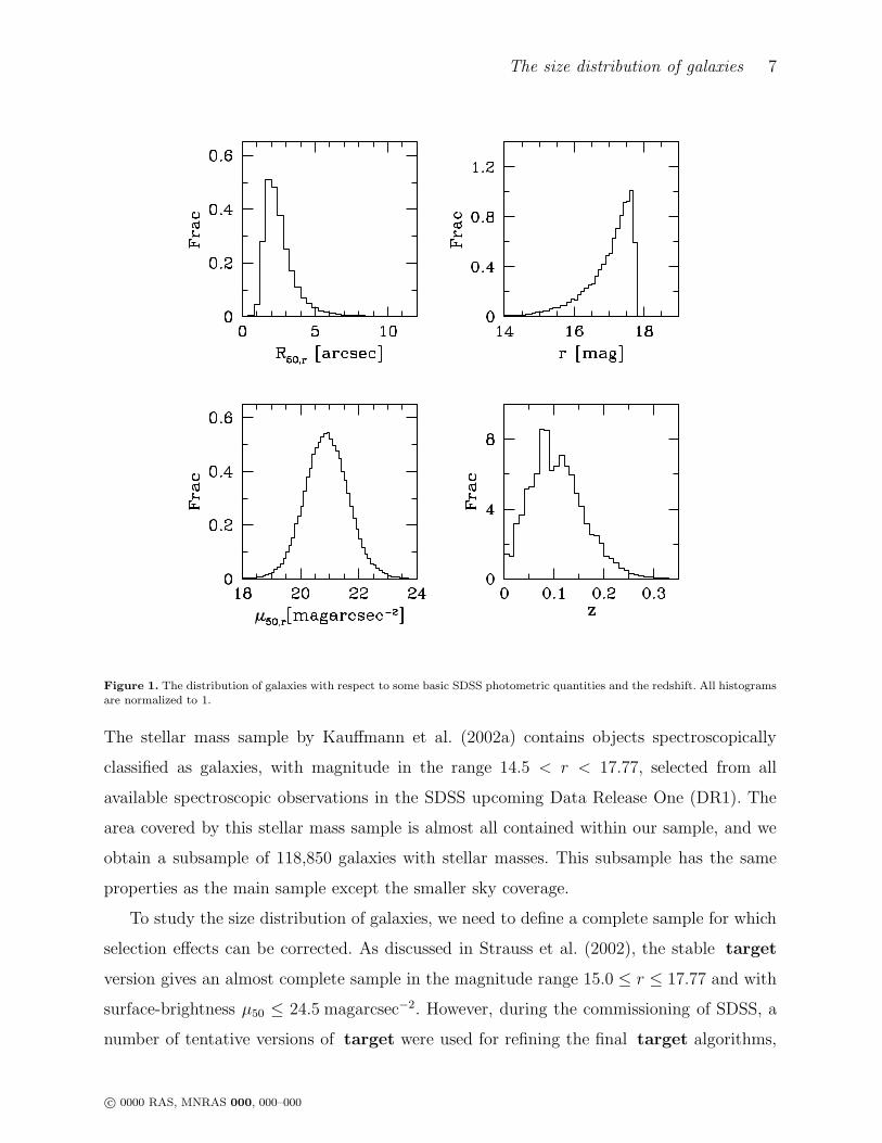
Figure 1 shows histograms of the basic quantities of our selected sample. The top-right
panel shows the galaxy distribution in r-band apparent magnitude r after correction for
foreground Galactic extinction using the reddening map of Schlegel, Finkbeiner and Davis
(1998). The abrupt cut at ∼ 17.77 mag is caused by the target selection criteria. The top-left
panel shows the distribution of the r-band Petrosian half-light radius R50,r. The distribution
of µ50,r, the r-band average surface-brightness within R50,r, is shown in the bottom-left panel.
Since the r-band is the reference band of the SDSS for model fitting and target selection,
our discussion of sample incompleteness will be based on the photometric properties in this
band. The redshifts z of the sample galaxies are obtained from the spectroscopic data, and
the distribution of galaxies with respect to z is shown in the bottom-right panel of Figure 1.
All the galaxies in this sample have Sersic parameters given by Blanton et al. (2002b).
c© 0000 RAS, MNRAS 000, 000–000
The size distribution of galaxies 7
Figure 1. The distribution of galaxies with respect to some basic SDSS photometric quantities and the redshift. All histogramsare normalized to 1.
The stellar mass sample by Kauffmann et al. (2002a) contains objects spectroscopically
classified as galaxies, with magnitude in the range 14.5 < r < 17.77, selected from all
available spectroscopic observations in the SDSS upcoming Data Release One (DR1). The
area covered by this stellar mass sample is almost all contained within our sample, and we
obtain a subsample of 118,850 galaxies with stellar masses. This subsample has the same
properties as the main sample except the smaller sky coverage.
To study the size distribution of galaxies, we need to define a complete sample for which
selection effects can be corrected. As discussed in Strauss et al. (2002), the stable target
version gives an almost complete sample in the magnitude range 15.0 ≤ r ≤ 17.77 and with
surface-brightness µ50 ≤ 24.5 magarcsec−2. However, during the commissioning of SDSS, a
number of tentative versions of target were used for refining the final target algorithms,
c© 0000 RAS, MNRAS 000, 000–000

8 Shen et al
and the trial targets have small differences in the magnitude and surface-brightness limits
(see EDR for detail). Therefore, to define a complete sample we need to consider selection
effects in more detail. Because galaxies with 23.0magarcsec−2 < µ50 < 24.5magarcsec−2 are
targeted only when the local and global sky values are within 0.05 magarcsec−2 (Strauss et
al. 2002), we set a lower surface-brightness limit at µlim = 23.0 magarcsec−2. As one can see
from the bottom-left panel of Fig. 1, the total number excluded by this selection criterion is
very small. Next, to avoid the contamination by bright stars, target rejects bright compact
objects with R50 < 2˝ and r < 15.0 (15.5 in target v 2 7). Because of this, we exclude all
galaxies brighter than 15.0 (15.5 for objects targeted by target v 2 7). As shown in Fig. 1,
only a small number of galaxies are excluded by this criterion also. Finally, the magnitude
limit (rmax) at the faint end varies across the sky in different versions of target. We take
this into account by treating rmax as a function of sky position (θ, φ).
A more important effect is that some galaxies are so small (compact) that either their
size measurements are seriously affected by the PSFs, or they are misclassified as stars by
target. As discussed by Strauss et al. (2002), very few true galaxies at the compact end are
missed by the target criteria. However, to take care of the seeing effects, we use only galaxies
with angular sizes R50 > Dmin, and we choose Dmin = 1.6′′ (i.e. 4 pixels). This choice, based
on the fact that the median seeing condition in SDSS is about 1.5′′, is conservative, because
the PSF is known quite accurately. In practice, this cut does not affect our results, as only
a relatively small fraction of galaxies is excluded (see the top-left panel of Fig.1). Finally
we also exclude a small number of galaxies with redshift z < 0.005, whose distances may be
severely contaminated by their peculiar velocities. In summary, our final complete sample
includes all galaxies with µ50 ≤ 23.0 magarcsec−2, rmin(θ, φ) ≤ r ≤ rmax(θ, φ), R50 ≥ 1.6′′
and z ≥ 0.005. This sample contains 138,521 galaxies, of which 99,786 have stellar masses.
2.4 Subsamples of galaxy types
In this paper we also wish to analyze the dependence of the size distribution on galaxy type,
so we need to adopt some criteria to classify galaxies.
There are attempts to classify SDSS galaxies into morphological classes through direct
inspection of the galaxy images (Shimasaku et al. 2001; Nakamura et al. 2003). While such
eye-ball classification should match the original Hubble morphological sequence, it is quite
tedious and has so far been carried out only for about 1500 big galaxies in the SDSS. However,
c© 0000 RAS, MNRAS 000, 000–000
The size distribution of galaxies 9
it has been suggested that some photometric and spectroscopic properties may be closely
correlated with the morphological type, and so can be used as morphology indicators. For
example, Shimasaku et al. (2001) show that the concentration c can be used to separate early-
type (E/S0) galaxies from late-type (Sa/b/c, Irr) galaxies. Using about 1500 galaxies with
eye-ball classifications, Nakamura et al. (2003) confirmed that c = 2.86 separates galaxies
at S0/a with a completeness of about 0.82 for both late and early types. For the Sersic
profile (Blanton et al. 2002b), the profile index n is uniquely related to the concentration
parameter, and so the value of n may also serve as a morphological indicator. Other profile
indicators of galaxy type include the exponential and de Vaucouleurs profile likelihoods, Pexp
and Pdev, given in the Photo output. Based on the broad band colors, Strateva et al. (2002)
suggested that the color criterion u∗−r∗ > 2.22 can separate early types (E/S0/Sa) from late
types (Sb/Sc/Irr). Blanton et al. (2002b) found that the color criteria 0.1(g−r) ∼ 0.7 [where
0.1(g−r) is the g−r color K-corrected to the redshift of 0.1] separates galaxies into two groups
with distinct properties. There are also attempts to classify SDSS galaxies according to their
spectral types, such as that based on the Principal Component Analysis (Yip et al. 2003)
and that on the 4000A spectral break index (Kauffmann et al. 2002b). It must be pointed
out, however, that all these simple type classifications have uncertainties and are only valid
in the statistical sense. For example, the profile and color indices can both be affected by
dust extinction, while the classifications based on spectra can be affected aperture biases
due to the finite (3′′ in diameter) of the fibers. Because of these uncertainties, we only divide
galaxies into a small number of subsamples according to types. More specifically, we use
c = 2.86 and n = 2.5 as two basic indicators to separate galaxies into early and late types.
With such a separation, most Sa galaxies are included in the late-type category. We also use
the color criterion, 0.1(g−r) = 0.7 for comparison. The n separation is set at 2.5, the average
between exponential profile (n = 1) and de Vaucouleurs profile (n = 4), which also gives
an early/late ratio similar to that given by the separator c = 2.86. We adopt the 0.1(g − r)
color rather than the u∗ − r∗ color, because the g-band photometry is currently better than
the u-band photometry in the SDSS and because the K-correction for the u-band is very
uncertain.
c© 0000 RAS, MNRAS 000, 000–000

10 Shen et al
3 THE SIZE DISTRIBUTION OF GALAXIES
In this section, we derive the size distribution as a function of luminosity and stellar mass
for galaxies of different types. Specifically, we first bin galaxies of a given type into small
bins of absolute magnitude (or mass). We then use a Vmax method to make corrections
for the incompleteness due to selection effects, and derive the conditional size distribution
function fi(R|Mi) for a given bin. Finally, we investigate the size distribution as a function
of luminosity (or stellar mass).
3.1 The Vmax correction of the selection effects
As described in the last section, our sample is selected to be complete only to some mag-
nitude, size and surface-brightness limits. In order to obtain the size distribution for the
galaxy population as a whole, we must make corrections for these selection effects. In this
paper we use the Vmax method to do this.
The basic idea of the Vmax method is to give each galaxy a weight which is proportional
to the inverse of the maximum volume (Vmax) within which galaxies identical to the one
under consideration can be observed. For a given galaxy with magnitude r, Petrosian half-
light radius R50, surface-brightness µ50, and redshift z, the selection criteria described in
the last section define the value of Vmax in the following way. First, the magnitude range
rmin ≤ r ≤ rmax corresponds to a maximum redshift zmax,m and a minimum redshift zmin,m:
dL(zmax,m) = dL(z)10−0.2(r−rmax) ; dL(zmin,m) = dL(z)10−0.2(r−rmin), (4)
where dL(z) is the luminosity distance at redshift z. Note that we have neglected the effects
of K-correction and luminosity evolution in calculating dL(zmax,m) and dL(zmin,m). In general,
the K-correction make a given galaxy fainter in the observed r-band if it is put at higher
redshift. The luminosity evolution has an opposite effect; it makes galaxies brighter at higher
redshift. We found that including these two opposing effects (each is about one magnitude
per unit redshift, see Blanton et al. 2002a; 2002c) has a negligible impact on our results.
The surface-brightness limit constrains the Vmax of a galaxy mainly through the dimming
effect. The maximum redshift at which a galaxy of surface-brightness µ50 at z can still be
observed with the limit surface-brightness µlim = 23.0 is given by
zmax,µ = (1 + z)10(23.0−µ50)
10 − 1. (5)
Here, again, K-correction and luminosity evolution are neglected. We have also neglected
c© 0000 RAS, MNRAS 000, 000–000

The size distribution of galaxies 11
possible color gradients in individual galaxies. The minimum size limit Dmin also defines a
maximum redshift zmax,R given by
dA(zmax,R)
dA(z)=
R50
1.6˝, (6)
where dA is the angular-diameter distance. The real maximum and minimum redshifts, zmax
and zmin, for a given galaxy are therefore given by
zmin = max(zmin,m, 0.005) ; zmax = min(zmax,m, zmax,µ, zmax,R), (7)
and the corresponding Vmax is
Vmax =1
4π
∫
dΩf(θ, φ)∫ zmax(θ,φ)
zmin(θ,φ)
d2A(z)
H(z)(1 + z)c dz , (8)
where H(z) is the Hubble constant at redshift z, c is the speed of light, f(θ, φ) is the sampling
fraction as a function of position on the sky, and Ω is the solid angle.
The apparent-magnitude limit only influences the number of galaxies at a given absolute-
magnitude, and so it does not matter when we analyze the size distribution for galaxies with
a given absolute magnitude. We can define a ‘conditional’ maximum volume,
V ∗max =
Vmax
(4π)−1∫
dΩf(θ, φ)∫ zmax,m(θ,φ)zmin(θ,φ) d2
A(z)H−1(z)(1 + z)−1c dz(9)
which takes values from 0 to 1, and gives the probability a galaxy with size R50 can be
observed at the given absolute magnitude. Given N galaxies in an absolute-magnitude (or
mass) bin M ± ∆M , the intrinsic conditional size distribution f(R|M) can be estimated
from
f(R|M) ∝N∑
i=1
1
V ∗max,i
if R − dR < Ri < R + dR, (10)
where Ri and V ∗max,i are the radius and the value of V ∗
max for the ith galaxy.
3.2 Size distribution: dependence on luminosity
In this subsection, we study the size distribution as a function of luminosity for galaxies of
different type. The absolute magnitude M is calculated from the observed apparent magni-
tude m using
M = m − DM(z) + 5 − K(z), (11)
where z is the redshift of the galaxy, DM(z) is the distance modulus and K(z) is the K-
correction. The distances are calculated from redshifts using a cosmology with mass density
c© 0000 RAS, MNRAS 000, 000–000
12 Shen et al
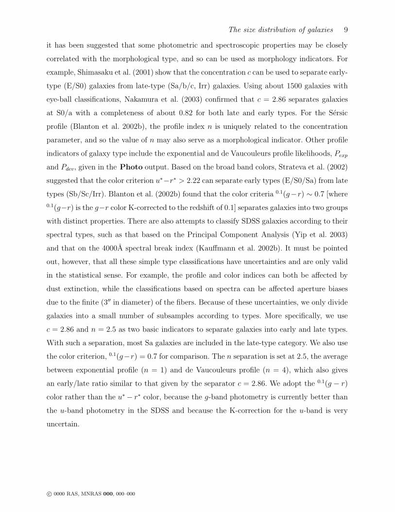
Figure 2. Histograms of Petrosian half-light radius R50 (in the r-band) for early-type (c > 2.86) galaxies in different Petrosianr-band absolute-magnitude bins. The dotted histograms show the raw distribution, while the solid histograms show the resultsafter Vmax correction for selection effects. The solid curves are obtained by fitting the sizes to a log-normal distribution throughthe maximum-likelihood method.
Ω0 = 0.3, cosmological constant ΩΛ = 0.7, and Hubble’s constant h = 0.7. The K-correction
is calculated based on the study of Blanton et al. (2002a).
In Figures 2 and 3 we show the histograms of Petrosian half-light radius R50 for galaxies
of different absolute magnitudes and types. We use c = 2.86 to separate galaxies, in which
case 32 percent of them are included in the early types. Galaxies of a given type are further
divided into absolute-magnitude bins with a width of 0.5mag. The dotted histograms show
the observed size distributions, obtained by directly counting the numbers of galaxies in given
size bins. The intrinsic distributions, obtained by using the V ∗max correction [see equation
(10)], are shown as the solid histograms. All the histograms are normalized to the unit area
in the space of Log (R50).
c© 0000 RAS, MNRAS 000, 000–000
The size distribution of galaxies 13
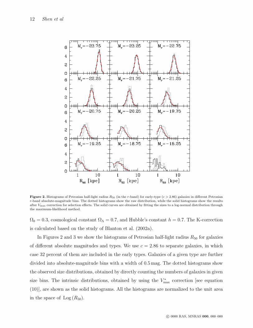
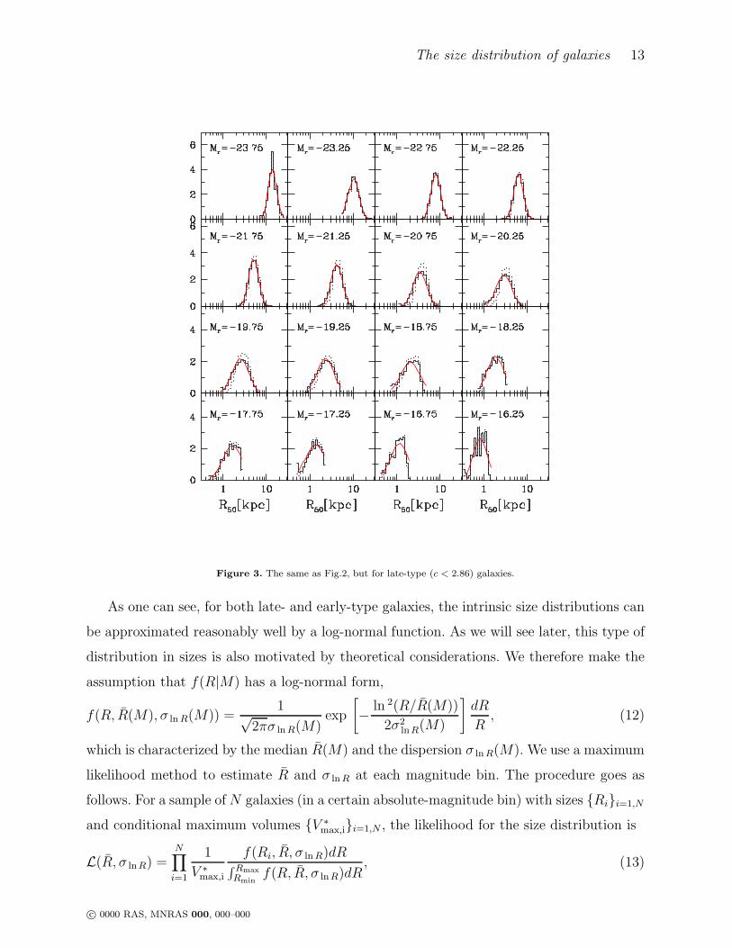
Figure 3. The same as Fig.2, but for late-type (c < 2.86) galaxies.
As one can see, for both late- and early-type galaxies, the intrinsic size distributions can
be approximated reasonably well by a log-normal function. As we will see later, this type of
distribution in sizes is also motivated by theoretical considerations. We therefore make the
assumption that f(R|M) has a log-normal form,
f(R, R(M), σ ln R(M)) =1√
2πσ ln R(M)exp
[
− ln 2(R/R(M))
2σ2lnR(M)
]
dR
R, (12)
which is characterized by the median R(M) and the dispersion σ ln R(M). We use a maximum
likelihood method to estimate R and σ ln R at each magnitude bin. The procedure goes as
follows. For a sample of N galaxies (in a certain absolute-magnitude bin) with sizes Rii=1,N
and conditional maximum volumes V ∗max,ii=1,N , the likelihood for the size distribution is
L(R, σ lnR) =N∏
i=1
1
V ∗max,i
f(Ri, R, σ ln R)dR∫ RmaxRmin
f(R, R, σ lnR)dR, (13)
c© 0000 RAS, MNRAS 000, 000–000

14 Shen et al
Figure 4. The median and dispersion of the distribution of Petrosian half-light radius R50 (in the r-band), as functions ofr-band Petrosian absolute magnitude, obtained by fitting a log-normal function. Results for late-type (c < 2.86) and early-type(c > 2.86) galaxies are shown as triangles and squares, respectively. The error bars represent the scatter among 20 bootstrapsamples. The solid curves are the fit of the R - M and σ ln R - M relations by equations (14), (15) and (16).
where Rmin and Rmax are the minimum and maximum radii that can be observed for the
luminosity bin in consideration, f(R, R, σ lnR) is the log-normal function with median R and
dispersion σ ln R given in equation (12). By maximizing this likelihood function, we obtain
the best estimates of R and σ lnR for each magnitude bin. The solid curves in Figures 2 and
3 show the results of the log-normal functions so obtained. As one can see, they provide very
good fits to the solid histograms.
Figure 4 shows R (upper panel) and σ ln R (lower panel) against the absolute magnitude.
Triangles and squares denote the results for late- and early-type galaxies, respectively. The
error bars are obtained from the scatter among 20 bootstrap samples. The small error bars
show the statistics one can get from the current sample. The number of faint early-type
c© 0000 RAS, MNRAS 000, 000–000

The size distribution of galaxies 15
galaxies is still too small to give any meaningful results (see the panel of Mr = 18.25 in
Fig. 1). This small number may not mean that the number of faint elliptical galaxies is
truly small; it may just reflect our definition of early- and late-type galaxies. Indeed, faint
elliptical galaxies seem to have surface-brightness profiles better described by an exponential
than a R1/4 law (Andredakis, Peletier & Balcells 1995; Kormendy & Bender 1996), and so
they will be classified as ‘late-type’ galaxies according to the c criterion because of their
small concentration.
As shown in Fig. 4, the dependence of R on the absolute magnitude is quite different
for early- and late-type galaxies. In general, the increase of R with luminosity is faster for
early-type galaxies. The R - M relation can roughly be described by a single power law for
bright early-type galaxies, while for late-type galaxies, the relation is significantly curved,
with brighter galaxies showing a faster increase of R with M . In the luminosity range where
R and σ ln R can be determined reliably, the dispersion has a similar trend with M for both
early- and late-type galaxies. An interesting feature in σ ln R is that it is significantly smaller
for galaxies brighter than −20.5 mag (in the r-band). As we will discuss in Section 4, these
observational results have important implications for the theory of galaxy formation.
To quantify the observed R - M and σ ln R - M relations, we fit them with simple analytic
formulae. For early-type galaxies, we fit R - M by,
Log (R/ kpc) = −0.4aM + b , (14)
where a and b are two fitting constants. For late-type galaxies, we fit the size-luminosity
relation and its dispersion by
Log (R/ kpc) = −0.4αM + (β − α) Log [1 + 10−0.4(M−M0)] + γ (15)
and
σ ln R = σ2 +(σ1 − σ2)
1 + 10−0.8(M−M0), (16)
where α, β, γ, σ1, σ2 and M0 are fitting parameters. Note that the value of M0 used in
equation (15) is determined by fitting the observed σ ln R - M relation [equation (16)], because
the fit of the R - M relation is not very sensitive to the value of M0. Thus, the relation
between R and the luminosity L is R ∝ La for early-type galaxies. For late-type galaxies,
R ∝ Lα, σ ln R = σ1 at the faint end (L ≪ L0, where L0 is the luminosity corresponding to
M0), and R ∝ Lβ , σ lnR = σ2 at the bright end (L ≫ L0). We use the least-square method
c© 0000 RAS, MNRAS 000, 000–000
16 Shen et al
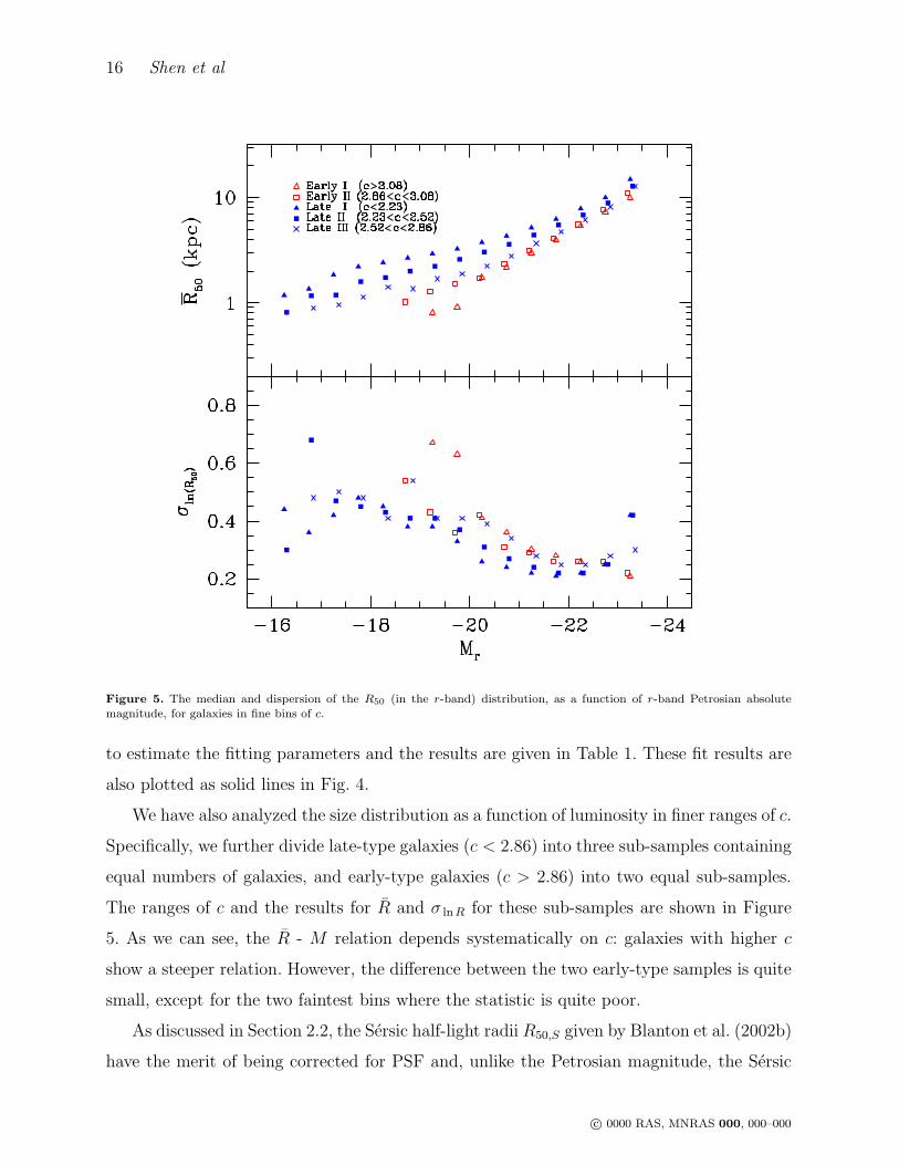
Figure 5. The median and dispersion of the R50 (in the r-band) distribution, as a function of r-band Petrosian absolutemagnitude, for galaxies in fine bins of c.
to estimate the fitting parameters and the results are given in Table 1. These fit results are
also plotted as solid lines in Fig. 4.
We have also analyzed the size distribution as a function of luminosity in finer ranges of c.
Specifically, we further divide late-type galaxies (c < 2.86) into three sub-samples containing
equal numbers of galaxies, and early-type galaxies (c > 2.86) into two equal sub-samples.
The ranges of c and the results for R and σ lnR for these sub-samples are shown in Figure
5. As we can see, the R - M relation depends systematically on c: galaxies with higher c
show a steeper relation. However, the difference between the two early-type samples is quite
small, except for the two faintest bins where the statistic is quite poor.
As discussed in Section 2.2, the Sersic half-light radii R50,S given by Blanton et al. (2002b)
have the merit of being corrected for PSF and, unlike the Petrosian magnitude, the Sersic
c© 0000 RAS, MNRAS 000, 000–000
The size distribution of galaxies 17
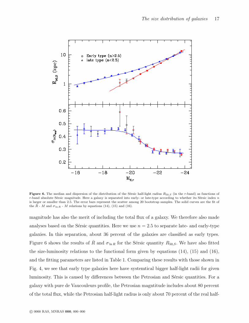
Figure 6. The median and dispersion of the distribution of the Sersic half-light radius R50,S (in the r-band) as functions ofr-band absolute Sersic magnitude. Here a galaxy is separated into early- or late-type according to whether its Sersic index nis larger or smaller than 2.5. The error bars represent the scatter among 20 bootstrap samples. The solid curves are the fit ofthe R - M and σ ln R - M relations by equations (14), (15) and (16).
magnitude has also the merit of including the total flux of a galaxy. We therefore also made
analyses based on the Sersic quantities. Here we use n = 2.5 to separate late- and early-type
galaxies. In this separation, about 36 percent of the galaxies are classified as early types.
Figure 6 shows the results of R and σ ln R for the Sersic quantity R50,S. We have also fitted
the size-luminosity relations to the functional form given by equations (14), (15) and (16),
and the fitting parameters are listed in Table 1. Comparing these results with those shown in
Fig. 4, we see that early type galaxies here have systemtical bigger half-light radii for given
luminosity. This is caused by differences between the Petrosian and Sersic quantities. For a
galaxy with pure de Vaucouleurs profile, the Petrosian magntitude includes about 80 percent
of the total flux, while the Petrosian half-light radius is only about 70 percent of the real half-
c© 0000 RAS, MNRAS 000, 000–000
18 Shen et al
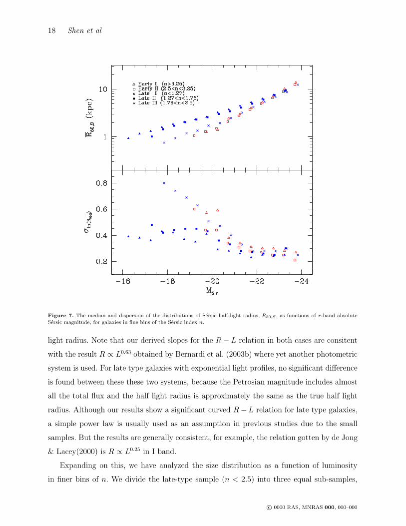
Figure 7. The median and dispersion of the distributions of Sersic half-light radius, R50,S , as functions of r-band absoluteSersic magnitude, for galaxies in fine bins of the Sersic index n.
light radius. Note that our derived slopes for the R − L relation in both cases are consitent
with the result R ∝ L0.63 obtained by Bernardi et al. (2003b) where yet another photometric
system is used. For late type galaxies with exponential light profiles, no significant difference
is found between these these two systems, because the Petrosian magnitude includes almost
all the total flux and the half light radius is approximately the same as the true half light
radius. Although our results show a significant curved R −L relation for late type galaxies,
a simple power law is usually used as an assumption in previous studies due to the small
samples. But the results are generally consistent, for example, the relation gotten by de Jong
& Lacey(2000) is R ∝ L0.25 in I band.
Expanding on this, we have analyzed the size distribution as a function of luminosity
in finer bins of n. We divide the late-type sample (n < 2.5) into three equal sub-samples,
c© 0000 RAS, MNRAS 000, 000–000

The size distribution of galaxies 19
Figure 8. The median and dispersion of the distribution of Sersic half-light radius R50,S , as a function of r-band Sersic absolutemagnitude. Triangles represent results for late-type galaxies [here defined to be those with 0.1(g − r) < 0.7], while the squaresare for early-type galaxies with 0.1(g − r) > 0.7. The error bars represent the scatter among 20 bootstrap samples.
and the early-type sample (n > 2.5) into two equal sub-samples. The ranges of n for these
sub-samples and the fitting results are shown in Figure 7. These results should be compared
with those shown in Fig. 5. While galaxies with higher n do show a steeper R - M relation,
the change of the trend with n is less systematic than with c. It seems that galaxies are
separated into two groups at n ∼ 1.7, and galaxies in each group have similar R - M
relations, independent of n. As shown by the two dimensional distribution of galaxies in the
space spanned by n and the 0.1(g−r) color (Blanton et al. 2002b), the cut at n = 1.7 roughly
corresponds to a color cut at 0.1(g − r) ≈ 0.7. The latter cut appears to separate E/S0/Sa
from Sb/Sc/Irr galaxies, as discussed in subsection 2.4.
For comparison, we consider separating galaxies according to the color criteria 0.1(g−r) =
0.7. The results are shown in Figure 8. In this case, since most Sa galaxies are classified as
c© 0000 RAS, MNRAS 000, 000–000
20 Shen et al
early-type galaxies, there are fewer bright late-type galaxies. Moreover, we begin to see faint
red galaxies (presumably faint ellipticals), which would be classified as ‘late-type’ galaxies
by the c and n criteria, because of their low concentrations. As one can see, the late-type
galaxies show approximately the same statistical properties as those in the c and n classifi-
cations. This is also true for bright early-type galaxies. Red galaxies with Mr ∼ −20 seem
to follow a parallel trend to late-type galaxies, although they are smaller at given absolute
magnitude. This is consistent with the fact that many dwarf ellipticals show exponential
surface-brightness profiles, have small sizes, and have size-luminosity scaling relations simi-
lar to that of spiral galaxies (e.g. Caon, Capaccioli & D’Onofrio 1993; Kormendy & Bender
1996; Guzman et al. 1997; Prugniel & Simien 1997; Gavazzi et al. 2001). Faint red galax-
ies with Mr > −19 seem to have almost constant size. Note that σ ln R - M show similar
dependence on M for both red and blue galaxies.
Since most of the concentrated galaxies have red colors while galaxies with low concentra-
tions can have both blue and red colors, it is interesting to examine the properties of galaxies
selected by both color and n. To do this, we consider a case where galaxies with n < 2.5 are
divided further into two subsamples according to the color criterion 0.1(g − r) = 0.7. The
results are shown in Figure 9. As we can see, B type galaxies (with low n and red color) show
a R-M relation which is closer to that of A type (high n) galaxies than that of C-type (blue
and low n). Note again that faint red galaxies have sizes almost independent of luminosity.
The σ lnR - M relations are similar for all three cases.
So far our discussion has been based on the r-band data. If galaxies possess significant
radial color gradients, the size of a galaxy may be different in different wavebands. Further-
more, if galaxies have different colors, the size distribution as a function of luminosity may
also be different in different wavebands. To test how significant these effects are, we have
analyzed the size distributions separately in the SDSS g, i and z bands, using either the
absolute magnitudes in the corresponding band or the absolute magnitudes in the r-band
to bin galaxies into luminosity sub-samples. The results are qualitatively the same as de-
rived from the r-band data. Similar conclusions for early type galaxies have been reached
by Bernardi et al. (2003b). As an example, we show in Figure 10 the results based on Sersic
radii and Sersic z-band magnitudes. The galaxies are also separated into late- and early-
type by the r-band Sersic index n = 2.5. The results of fitting the R - M and σ ln R - M
relations are presented in Table 1. Because of the long wavelength involved in the z-band
c© 0000 RAS, MNRAS 000, 000–000
The size distribution of galaxies 21
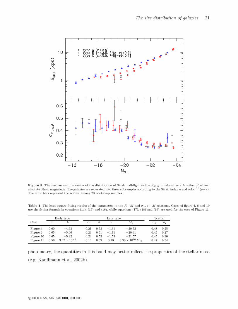
Figure 9. The median and dispersion of the distribution of Sersic half-light radius R50,S in r-band as a function of r-bandabsolute Sersic magnitude. The galaxies are separated into three subsamples according to the Sersic index n and color 0.1(g−r).The error bars represent the scatter among 20 bootstrap samples.
Table 1. The least square fitting results of the parameters in the R - M and σ lnR - M relations. Cases of figure 4, 6 and 10use the fitting formula in equations (14), (15) and (16), while equations (17), (18) and (19) are used for the case of Figure 11.
Early type Late type ScatterCase a b α β γ M0 σ1 σ2
Figure 4 0.60 −4.63 0.21 0.53 −1.31 −20.52 0.48 0.25Figure 6 0.65 −5.06 0.26 0.51 −1.71 −20.91 0.45 0.27Figure 10 0.65 −5.22 0.23 0.53 −1.53 −21.57 0.45 0.30Figure 11 0.56 3.47 × 10⁻⁵ 0.14 0.39 0.10 3.98 × 10¹⁰ M⊙ 0.47 0.34
photometry, the quantities in this band may better reflect the properties of the stellar mass
(e.g. Kauffmann et al. 2002b).
c© 0000 RAS, MNRAS 000, 000–000
22 Shen et al
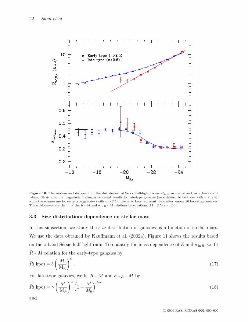
Figure 10. The median and dispersion of the distribution of Sersic half-light radius R50,S in the z-band, as a function ofz-band Sersic absolute magnitude. Triangles represent results for late-type galaxies (here defined to be those with n < 2.5),while the squares are for early-type galaxies (with n > 2.5). The error bars represent the scatter among 20 bootstrap samples.The solid curves are the fit of the R - M and σ ln R - M relations by equations (14), (15) and (16).
3.3 Size distribution: dependence on stellar mass
In this subsection, we study the size distribution of galaxies as a function of stellar mass.
We use the data obtained by Kauffmann et al. (2002a). Figure 11 shows the results based
on the z-band Sersic half-light radii. To quantify the mass dependence of R and σ ln R, we fit
R - M relation for the early-type galaxies by
R( kpc) = b
(
M
M⊙
)a
. (17)
For late-type galaxies, we fit R - M and σ ln R - M by
R( kpc) = γ
(
M
M⊙
)α (
1 +M
M0
)β−α
(18)
and
c© 0000 RAS, MNRAS 000, 000–000
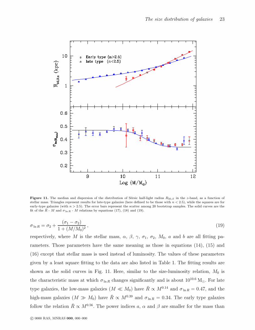
The size distribution of galaxies 23
Figure 11. The median and dispersion of the distribution of Sersic half-light radius R50,S in the z-band, as a function ofstellar mass. Triangles represent results for late-type galaxies (here defined to be those with n < 2.5), while the squares are forearly-type galaxies (with n > 2.5). The error bars represent the scatter among 20 bootstrap samples. The solid curves are thefit of the R - M and σ ln R - M relations by equations (17), (18) and (19).
σ ln R = σ2 +(σ1 − σ2)
1 + (M/M0)2, (19)
respectively, where M is the stellar mass, α, β, γ, σ1, σ2, M0, a and b are all fitting pa-
rameters. Those parameters have the same meaning as those in equations (14), (15) and
(16) except that stellar mass is used instead of luminosity. The values of these parameters
given by a least square fitting to the data are also listed in Table 1. The fitting results are
shown as the solid curves in Fig. 11. Here, similar to the size-luminosity relation, M0 is
the characteristic mass at which σ ln R changes significantly and is about 1010.6 M⊙. For late
type galaxies, the low-mass galaxies (M ≪ M0) have R ∝ M0.14 and σ ln R = 0.47, and the
high-mass galaxies (M ≫ M0) have R ∝ M0.39 and σ ln R = 0.34. The early type galaxies
follow the relation R ∝ M0.56. The power indices a, α and β are smaller for the mass than
c© 0000 RAS, MNRAS 000, 000–000
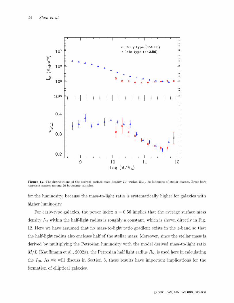
24 Shen et al
Figure 12. The distributions of the average surface-mass density I50 within R50,z as functions of stellar masses. Error barsrepresent scatter among 20 bootstrap samples.
for the luminosity, because the mass-to-light ratio is systematically higher for galaxies with
higher luminosity.
For early-type galaxies, the power index a = 0.56 implies that the average surface mass
density I50 within the half-light radius is roughly a constant, which is shown directly in Fig.
12. Here we have assumed that no mass-to-light ratio gradient exists in the z-band so that
the half-light radius also encloses half of the stellar mass. Moreover, since the stellar mass is
derived by multiplying the Petrosian luminosity with the model derived mass-to-light ratio
M/L (Kauffmann et al., 2002a), the Petrosian half light radius R50 is used here in calculating
the I50. As we will discuss in Section 5, these results have important implications for the
formation of elliptical galaxies.
c© 0000 RAS, MNRAS 000, 000–000
The size distribution of galaxies 25
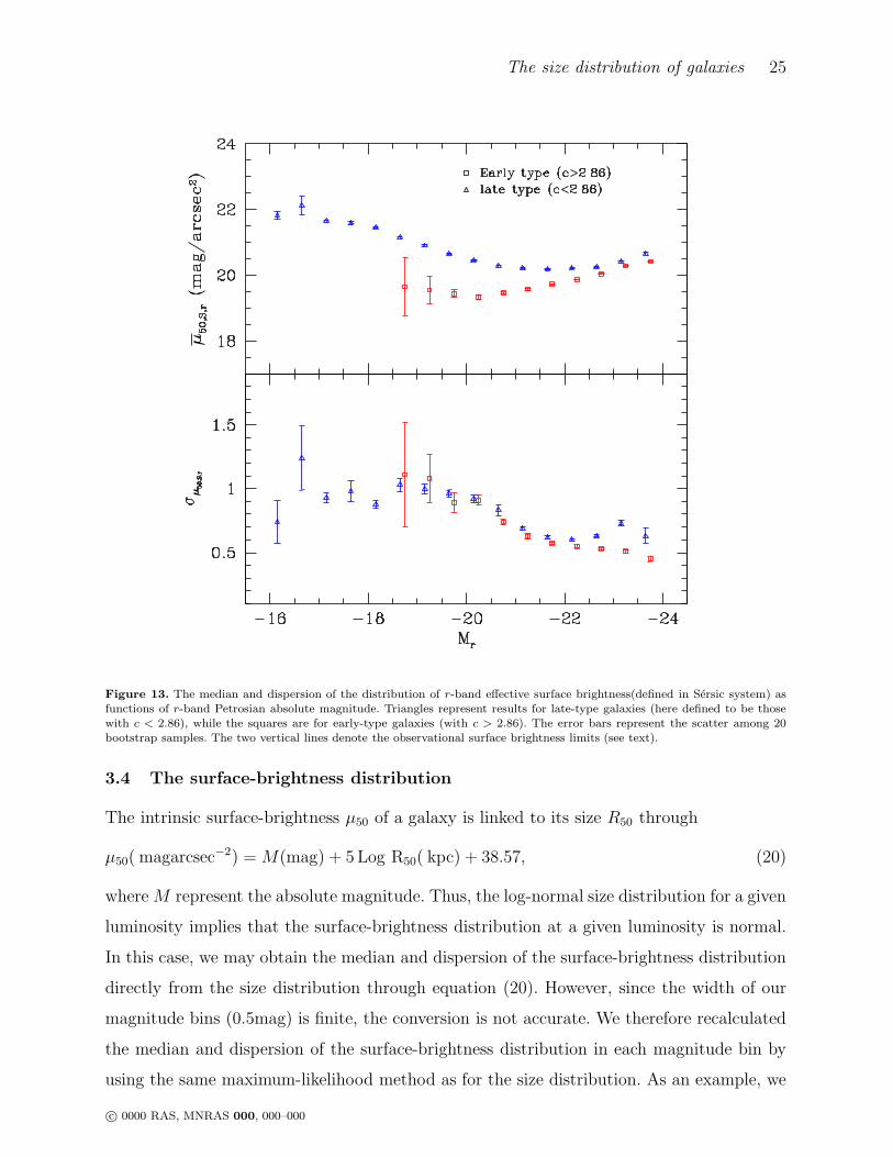
Figure 13. The median and dispersion of the distribution of r-band effective surface brightness(defined in Sersic system) asfunctions of r-band Petrosian absolute magnitude. Triangles represent results for late-type galaxies (here defined to be thosewith c < 2.86), while the squares are for early-type galaxies (with c > 2.86). The error bars represent the scatter among 20bootstrap samples. The two vertical lines denote the observational surface brightness limits (see text).
3.4 The surface-brightness distribution
The intrinsic surface-brightness µ50 of a galaxy is linked to its size R50 through
µ50( magarcsec−2) = M(mag) + 5 Log R50( kpc) + 38.57, (20)
where M represent the absolute magnitude. Thus, the log-normal size distribution for a given
luminosity implies that the surface-brightness distribution at a given luminosity is normal.
In this case, we may obtain the median and dispersion of the surface-brightness distribution
directly from the size distribution through equation (20). However, since the width of our
magnitude bins (0.5mag) is finite, the conversion is not accurate. We therefore recalculated
the median and dispersion of the surface-brightness distribution in each magnitude bin by
using the same maximum-likelihood method as for the size distribution. As an example, we
c© 0000 RAS, MNRAS 000, 000–000

26 Shen et al
show the r-band surface-brightness distribution in Figure 13. The surface-brightness used
here is defined in the Sersic system, i.e. the average surface brightness inside the Sersic
half-light radius, but galaxies are labelled by their Petrosian magnitudes. The reason for
this is that the luminosity function we are going to use to derive the integrated surface
brightness distribution is based on Petrosian magnitudes. As before, galaxies are separated
into late- and early-type galaxies at c = 2.86. As one can see from Fig. 13, the brighter late-
type galaxies have systematically higher surface-brightness while the trend is the opposite
for bright early-type galaxies. This is the well-known Kormendy relation (1977). Another
feature clearly seen is that the mean value of the surface-brightness is almost independent of
luminosity for bright late-type galaxies, which is consistent with the Freeman disk (Freeman
1970). For dwarf late-type galaxies, the surface brightness shows a strong increase with
increasing of luminosity in the range −20 < Mr < −18. But the median value of the surface
brightness is consistent with being constant in the luminosity range −16 < Mr < −18.
However, this result should be treated with caution, because the median value is already
quite close to the limit 23.0 magarcsec−2. Any incompleteness near 23.0 magarcsec−2 can
bias the median to a lower value (i.e. higher surface brightness).
With the conditional surface-brightness distribution function f(µ50|M), we can calculate
the number density of galaxies at any given surface-brightness µ50 by integrating over the
luminosity function φ(M):
φ(µ50) =∫
φ(M)f(µ50|M) dM . (21)
The luminosity functions of early- and late-type galaxies separated at c = 2.86 have recently
been given by Nakamura et al. (2003) based on the Petrosian magnitudes. As shown in
Fig. 13, our conditional surface-brightness distribution is reliably determined only in the
luminosity range −24 < Mr < −16 for late-type galaxies, and in −24 < Mr < −19 for early-
type galaxies. Therefore, we set the bright end of the integration in equation (21) to be Mr =
−24 and carry out the integration from a number of low-luminosity limits. The median and
dispersion of the surface-brightness distribution at any given magnitude are obtained from
a linear interpolation between adjacency magnitude bins. The results are shown on Figure
14 with the faint-end limits labelled on the corresponding curves. The two vertical lines at
18.0 and 23.0 magarcsec−2 correspond to the observational surface brightness limits(defined
in Petrosian system) of our sample. The bright limit 18.0 magarcsec−2 corresponds to the
brightest galaxies (r = 15.0) with sizes at the lower limit (1.6′′).
c© 0000 RAS, MNRAS 000, 000–000

The size distribution of galaxies 27
Figure 14. The surface-brightness distribution for late- (c < 2.86) and early-type (c > 2.86) galaxies in different luminosityranges, obtained by convolving the observed luminosity function φ(L) with the conditional surface-brightness distributionf(µ50|L) shown in Fig. 13.
As one can see from the figure, there may be many compact early-type galaxies that are
not included in our sample. For late-type galaxies, the surface-brightness shows a narrow
normal distribution for bright galaxies (i.e. the Freeman disk). When more dwarf galaxies
are included, low surface-brightness galaxies may contribute a large fraction of the total
numbers of galaxies. Unfortunately, the current data cannot give a stringent constraint on
the number density of low-surface brightness galaxies because the results for very faint
galaxies (Mr > −16) are uncertain. However, the fact that galaxies with the lowest surface
brightness are predominantly of low luminosity suggests that such low-surface brightness
galaxies contribute little to the luminosity density of the universe. A similar conclusion has
been reached in earlier analysis (e.g. de Jong & Lacey 2000; Cross & Driver 2002; Blanton
et al. 2001).
c© 0000 RAS, MNRAS 000, 000–000
28 Shen et al
4 THEORETICAL EXPECTATIONS
In the preceding sections we have seen that the current SDSS data can be used to derive
good statistics for the size distribution of galaxies and its dependence on luminosity, stellar
mass, concentration and color. In this section, we examine whether or not these observational
results can be accommodated in the current paradigm of galaxy formation.
4.1 Late – type galaxies
Let us start with late-type (spiral) galaxies. A spiral galaxy generally consists of a rotation-
ally supported thin disk, and an ellipsoidal bu lge which rotates relatively slowly.
4.1.1 The disk component
According to current theory of galaxy formation, galaxy disks are formed as gas with some
initial angular momentum cools and contracts in dark matter haloes. Our model of disk
formation follows that described in Mo, Mao & White (1998 hereafter MMW). The model
assumes spherical dark haloes with density profile given by Navarro, Frenk & White (1997,
hereafter NFW):
ρ(r) =ρ0
(r/rs)(1 + r/rs)2, (22)
where rs is a characteristic radius, and ρ0 is a characteristic density. The halo radius r200 is
defined so that the mean density within it is 200 times the critical density. It is then easy
to show that r200 is related to the halo mass Mh by
r200 =G1/3M
1/3h
[10H(z)]2/3, (23)
where H(z) is the is the Hubble constant at redshift z. The total angular momentum of a
halo, J , is usually written in terms of the spin parameter,
λ = J |E|1/2G−1M−5/2h , (24)
where E is the total energy of the halo. N -body simulations show that the distribution of
halo spin parameter λ is approximately log-normal,
p(λ) dλ =1√
2πσ ln λ
exp
[
− ln 2(λ/λ)
2σ2lnλ
]
dλ
λ, (25)
with λ ∼ 0.04 and σ ln λ ≈ 0.5 (Warren et al. 1992; Cole & Lacey 1996; Lemson & Kauffmann
1999).
We assume that the disk that forms in a halo has mass Md related to the halo mass by
c© 0000 RAS, MNRAS 000, 000–000
The size distribution of galaxies 29
Md = mdMh , (26)
and has angular momentum Jd related to the halo spin by
Jd = jdJ , (27)
where md and jd give the fractions of mass and angular-momentum in the disk. Assuming
that the disk has an exponential surface density profile and that the dark halo responds to
the growth of the disk adiabatically, the disk scale-length Rd can be written as
Rd =1√2
(
jd
md
)
λr200fr , (28)
where fr is a factor that depends both on halo profile and on the action of the disk (see
MMW for details). As shown in MMW, for a given halo density profile, fr depends both on
md and on λd ≡ (jd/md)λ, but the dependence on λd is not very strong. Thus, if jd/md is
constant, the log-normal distribution of λ will lead to a size distribution which is roughly
log-normal.
4.1.2 The bulge component
Our empirical knowledge about the formation of galaxy bulges is still very limited (e.g. Wyse,
Gilmore & Franx 1997). Currently there are two competing scenarios in the literature, one
is the merging scenario and the other is based on disk instability.
In the merging scenario, galaxy bulges, like elliptical galaxies, are assumed to form
through the mergers of two or more galaxies (Toomre & Toomre 1972). Subsequent accretion
of cold gas may form a disk around the existing bulge, producing a bulge/disk system like
a spiral galaxy (e.g. Kauffmann, White & Guiderdoni 1993; Kauffmann 1996; Baugh, Cole
& Frenk 1996; Jablonka, Martin & Arimoto 1996; Gnedin, Norman & Ostriker, 2000). In
this scenario, the formation of the bulge is through a violent process prior to the formation
of the disk, and so the properties of the bulge component are not expected to be closely
correlated with those of the disk that forms subsequently.
In the disk-instability scenario, low-angular momentum material near the centre of a
disk is assumed to form a bar due to a global instability; the bar is then transformed into
a bulge through a buckling instability (e.g. Kormendy 1989; Norman, Sellwood & Hasan
1996; Mao & Mo 1998; van den Bosch 1998; Noguchi 2000). The first of these instabilities is
well documented through direct simulation, the second less so. According to both N -body
c© 0000 RAS, MNRAS 000, 000–000
30 Shen et al
simulations (Efstathiou, Lake & Negroponte 1982) and analytic models (e.g. Christodoulou,
Shlosman & Tohline 1995) disks may become globally unstable when
ǫ ≡ Vm
(GMd/Rd)1/2
< ǫ0 , (29)
where Vm is the maximum rotation velocity of the disk, and ǫ0 ∼ 1. As discussed in MMW,
for a disk in a NFW halo, this criterion can approximately be written as md > λd. Thus, for
given λd, there is a critical value md,c for md above which the disk is unstable. If the overall
stellar mass fraction mg (defined as ratio of total stellar mass to total halo mass) is smaller
than md,c, the disk is stable and there is no bulge formation in this scenario. In this case,
mb = 0 and md = mg. Here, mb is the bulge fraction, which links the mass of the bulge to
the halo mass,
Mb = mbMh . (30)
If mg > md,c, we assume that the bulge mass is such that the disk has ǫ = ǫ0, i.e. the disk is
marginally unstable. In this case, md = md,c and mb = mg − md,c. Note that the gravity of
the bulge component must be taken into account when calculating ǫ. To do this, we include
a bulge component in the gravitational potential following MMW. For given mg and λd, we
then solve for mb and md iteratively.
To proceed further, we assume the angular momentum of the bulge to be negligible.
There are two ways in which the bulge may end up with little angular momentum: the first
is that it formed from halo material which initially had low specific angular momentum;
the second is that the bulge material lost most of its angular momentum to the halo and
the disk during formation. In the first case, we assume that the specific angular momentum
of the final disk is the same as that of the dark matter, so that jd = md. In the second
case, the final angular momentum of the disk depends on how much of the bulge’s initial
angular momentum it absorbs. Numerical simulations by Klypin, Zhao & Somerville (2002)
suggest that angular momentum loss is primarily to the disk for bulges that form through
bar instability. In general, we assume a fraction of fJ of the bulge angular momentum is
transferred to the disk component, and so Jd = (md + fJmb)J . Thus the effective spin
parameter for the disk is
λd = λ(1 + fJmb/md) , (31)
and we use this spin to calculate the disk size.
To complete our description of the disk component, we also need to model the size of the
c© 0000 RAS, MNRAS 000, 000–000

The size distribution of galaxies 31
bulge. Since current models of bulge formation are not yet able to make reliable predictions
about the size-mass relation, we have to make some assumptions based on observation.
Observed galaxy bulges have many properties similar to those of elliptical galaxies. We
therefore consider a model in which galaxy bulges follow the same size-mass relation as
early-type galaxies. Specifically, we assume that bulges with masses higher than 2×10¹⁰ M⊙
have de Vaucouleurs profiles and have a size-mass relation given by equation (17). For less
massive bulges, we adopt exponential profiles and two models for the size-mass relation. In
the first model, low-mass bulges follow a size-mass relation which is parallel to that of faint
late-type galaxies but has a lower zero point (so that it joins smoothly to the relation for
giant ellipticals at M = 2 × 10¹⁰ M⊙), i.e.
Log (Re/ kpc) =
0.56 Log (Mb) − 5.54 for Mb > 2 × 10¹⁰ M⊙
0.14 Log (Mb) − 1.21 for Mb < 2 × 10¹⁰ M⊙
, (32)
where Re is the effective radius of the bulge. This model is motivated by the fact that
dwarf ellipticals obey a size-luminosity relation roughly parallel to that of spiral galaxies
(Kormendy & Bender 1996; Guzman et al. 1997; see Figures 7 to 9). In the second model,
we assume a size-mass relation which is an extrapolation of that for the massive ellipticals,
i.e.
Log (Re/ kpc) = 0.56 Log (Mb) − 5.54 . (33)
In this case, faint bulges are small and compact, like compact ellipticals (Kormendy 1985;
Guzman et al. 1997). For simplicity, we do not consider the scatter in the size-mass relation
in either case.
With the mass and size known for both the disk and bulge components, we can obtain
the surface density profile of the model galaxy by adding up the surface density profiles of
the two components:
I(r) = Id(r) + Ib(r) , (34)
from which one can estimate the half-mass radius for each model galaxy.
4.1.3 The value of mg
If all the gas in a halo can settle to halo centre to form a galaxy, then mg ∼ ΩB,0/Ω0. For
the cosmological model adopted here this would imply mg ∼ 0.13, much larger than most
estimates of the baryon fraction in galaxies. In reality, not all the gas associated with a halo
c© 0000 RAS, MNRAS 000, 000–000
32 Shen et al
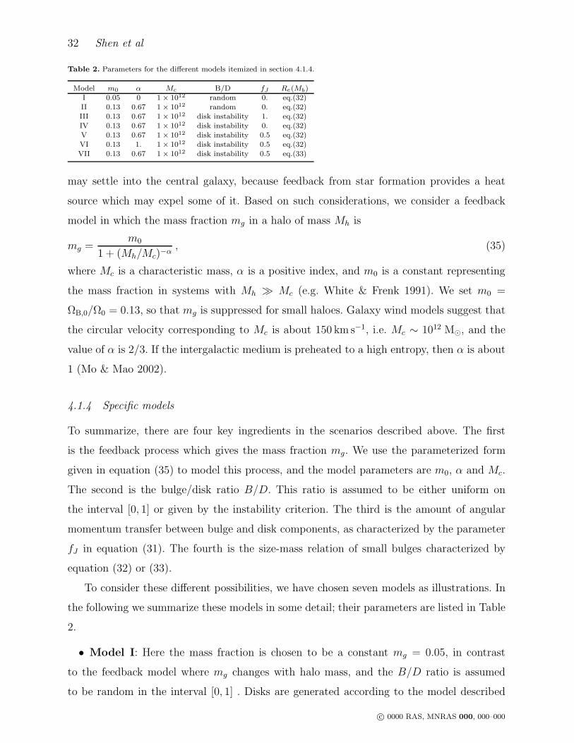
Table 2. Parameters for the different models itemized in section 4.1.4.
Model m0 α Mc B/D fJ Re(Mb)I 0.05 0 1 × 10¹² random 0. eq.(32)II 0.13 0.67 1 × 10¹² random 0. eq.(32)III 0.13 0.67 1 × 10¹² disk instability 1. eq.(32)IV 0.13 0.67 1 × 10¹² disk instability 0. eq.(32)V 0.13 0.67 1 × 10¹² disk instability 0.5 eq.(32)VI 0.13 1. 1 × 10¹² disk instability 0.5 eq.(32)VII 0.13 0.67 1 × 10¹² disk instability 0.5 eq.(33)
may settle into the central galaxy, because feedback from star formation provides a heat
source which may expel some of it. Based on such considerations, we consider a feedback
model in which the mass fraction mg in a halo of mass Mh is
mg =m0
1 + (Mh/Mc)−α, (35)
where Mc is a characteristic mass, α is a positive index, and m0 is a constant representing
the mass fraction in systems with Mh ≫ Mc (e.g. White & Frenk 1991). We set m0 =
ΩB,0/Ω0 = 0.13, so that mg is suppressed for small haloes. Galaxy wind models suggest that
the circular velocity corresponding to Mc is about 150 km s−1, i.e. Mc ∼ 1012 M⊙, and the
value of α is 2/3. If the intergalactic medium is preheated to a high entropy, then α is about
1 (Mo & Mao 2002).
4.1.4 Specific models
To summarize, there are four key ingredients in the scenarios described above. The first
is the feedback process which gives the mass fraction mg. We use the parameterized form
given in equation (35) to model this process, and the model parameters are m0, α and Mc.
The second is the bulge/disk ratio B/D. This ratio is assumed to be either uniform on
the interval [0, 1] or given by the instability criterion. The third is the amount of angular
momentum transfer between bulge and disk components, as characterized by the parameter
fJ in equation (31). The fourth is the size-mass relation of small bulges characterized by
equation (32) or (33).
To consider these different possibilities, we have chosen seven models as illustrations. In
the following we summarize these models in some detail; their parameters are listed in Table
2.
• Model I: Here the mass fraction is chosen to be a constant mg = 0.05, in contrast
to the feedback model where mg changes with halo mass, and the B/D ratio is assumed
to be random in the interval [0, 1] . Disks are generated according to the model described
c© 0000 RAS, MNRAS 000, 000–000
The size distribution of galaxies 33
in subsection 4.1.1, and bulges are assigned sizes according to equation (32). No angular-
momentum transfer from the bulge component to the disk is assumed.
• Model II: Here mg is assumed to follow equation (35), with m0 = 0.13, α = 2/3, and
Mc = 1012 M⊙. Other assumptions are the same as Model I.
• Model III: In this model mg is assumed to follow equation (35), with m0 = 0.13,
α = 2/3, and Mc = 1012 M⊙. Bulges are generated based on disk instability. All of the initial
angular momentum of the bulge is assumed to be transferred to the disk, i.e. fJ = 1. The
size-mass relation of the bulge component follows equation (32).
• Model IV: This model is the same as Model III, except that there is no angular
momentum transfer, i.e. fJ = 0.
• Model V: This model is also the same as Model III, except that half of the initial
angular momentum of the bulge material is transferred into the disk (i.e. fJ = 0.5).
• Model VI: This model is the same as Model V, except that α is assumed to be 1
instead of 2/3.
• Model VII: This model is the same as Model V, except that the size-mass relation of
bulge is equation (33) instead of Eq. (32)
4.1.5 Model predictions
We use Monte-Carlo simulations to generate galaxy samples for each of the models described
above. To do this, we first use the Press-Schechter (1974) formalism to generate 50,000 dark
matter haloes at redshift zero with masses (parameterized by circular velocity Vc) in the
range 35 km s−1 < Vc < 350 km s−1 and with a log-normal spin parameter distribution with
λ = 0.03 and σ ln λ = 0.45 (see equation 25).
We then use equations (23) – (35) to calculate the sizes and masses of the disk and
bulge for each galaxy. Finally, we combine the disk and bulge of each galaxy to calculate its
half-mass radius. As for the observational data, we sort galaxies into stellar mass bins and
calculate the median and dispersion of the size distribution as functions of stellar mass.
Figure 15 compares results for the seven models with the observational data for the
z-band Sersic half-light radii of late-type galaxies (n < 2.5) as function of stellar masses.
As one can see, if mg is assumed to be a constant, (Model I), the predicted median size-
mass relation is R ∝ M1/3, which is completely inconsistent with observations of low mass
galaxies. The predicted σ lnR is also too large. When mg is assumed to change with halo mass
c© 0000 RAS, MNRAS 000, 000–000

34 Shen et al
observationModel IModel II
Model IIIModel IVModel V
Model VIModel VII
Figure 15. The median and dispersion of the distribution of half-mass radius of spiral galaxies predicted by different modelsin comparison with the observed distribution of the z-band Sersic half-light radius as function of stellar mass (Fig. 11).Observational results are shown only for galaxies with n < 2.5. The models are described in detail in section 4.1.4 and modelparameters are listed in Table 2.
as suggested by the feedback scenario (Model II), the predicted shape of R - M is similar to
that observed for low mass galaxies, but the predicted median sizes are too small for high
mass galaxies. The predicted dispersion is also too big for high mass galaxies. If bulges are
assumed to form through disk instability and if fJ = 1 (Model III), the predicted scatter
follows the observations, but the predicted median sizes are too big for massive galaxies.
On the other hand, if no angular momentum is transferred, i.e. fJ = 0 (Model IV), the
predicted median size is smaller at the high mass end and the predicted scatter becomes
systematically higher. To match the observed behavior of the median and the dispersion
simultaneously, fJ ∼ 0.5 seems to be required (Model V). Changing the value of α from 2/3
to 1 (Model VI) gives a median size which is slightly too high for low-mass galaxies. If the
c© 0000 RAS, MNRAS 000, 000–000
The size distribution of galaxies 35
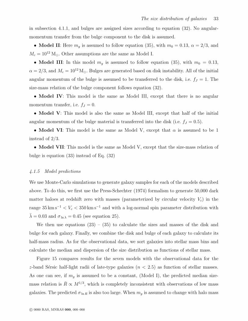
Figure 16. The prediction of Model V for the average bulge/disk ratios for galaxies with different stellar masses.
size-mass relation for small bulges is assumed to be an extension of that for big ellipticals
(Model VII), higher scatter is predicted for low mass galaxies.
Given that Model V reproduces the observed R - M and σ ln R - M relations, it is inter-
esting to look at other predictions of the model. In this case, the bulge/disk ratio depends on
the mass of the halo. A larger halo mass gives a larger value of mg and, in the disk-instability
model, this implies a larger bulge fraction. Hence we expect B/D to increase with galaxy
mass. Figure 16 shows the mean B/D ratio as a function of M according to Model V. The
predicted trend is consistent with the observed correlation between B/D and galaxy mass
(e.g. Roberts & Haynes 1994).
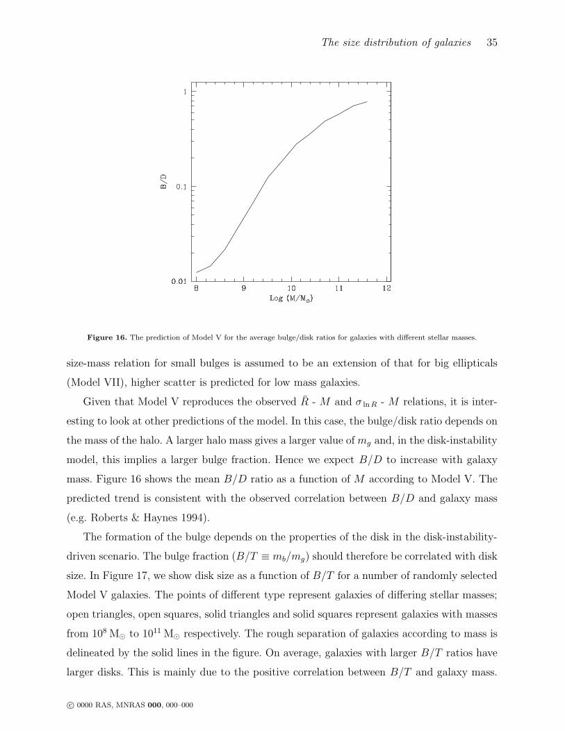
The formation of the bulge depends on the properties of the disk in the disk-instability-
driven scenario. The bulge fraction (B/T ≡ mb/mg) should therefore be correlated with disk
size. In Figure 17, we show disk size as a function of B/T for a number of randomly selected
Model V galaxies. The points of different type represent galaxies of differing stellar masses;
open triangles, open squares, solid triangles and solid squares represent galaxies with masses
from 108 M⊙ to 1011 M⊙ respectively. The rough separation of galaxies according to mass is
delineated by the solid lines in the figure. On average, galaxies with larger B/T ratios have
larger disks. This is mainly due to the positive correlation between B/T and galaxy mass.
c© 0000 RAS, MNRAS 000, 000–000
36 Shen et al
Figure 17. The prediction of Model V for the relation between disk scale-length and bulge/total mass ratio for late-typegalaxies. The points with different symbols represent galaxies in different mass ranges (as shown by the solid lines).
For a given stellar mass, galaxies with large B/T ratios have smaller disks. This is consistent
with the observational results of de Jong (1996). If the bulge/disk ratio is assumed to be
random, as in Models I and II, disk size is independent of B/T .
4.2 Early-type galaxies
Currently the most appealing model for the formation of elliptical galaxies assumes they
result from the merging of smaller systems. Numerical simulations have shown that mergers
of disk galaxies of similar mass do indeed produce remnants resembling elliptical galaxies
(e.g. Negroponte & White 1983; Hernquist 1992). However, it seems unlikely that every
elliptical is the remnant of a merger between two similar spirals drawn from the observed
local population. On the one hand, the stellar population of early-type galaxies is found
to be so old that the typical star formation epoch must be at z > 2 (e.g. Bernardi et al.
1998, 2003d; Thomas, Maraston & Bender 2002). On the other hand, detailed modelling of
the merger histories of galaxies in a CDM universe suggests that each elliptical obtains its
stars from progenitors covering a wide range in stellar mass, that the effective number of
progenitors increases weakly with the mass of the elliptical, that the last major merging event
is typically around redshift unity but with a wide dispersion, and that the progenitors may
c© 0000 RAS, MNRAS 000, 000–000

The size distribution of galaxies 37
Figure 18. Model predictions for the size distribution of early type galaxies. The solid lines assume ellipticals to be built byrepeated merging from a population of small progenitors, while the dotted lines show a model where each elliptical forms fromthe merger of two similar, late type galaxies. The observed size distribution of early type galaxies (n > 2.5) is reproduced fromFig. 11 for comparison.
have been gas-rich, producing a substantial fraction of the observed stars during merger
events (Kauffmann 1996; Baugh et al. 1996; Kauffmann & Charlot 1998; Kauffmann &
Haehnelt 2000). Rather than treating the detailed merger statistics of CDM models, we here
contrast two simpler models, one where ellipticals are built up by random mergers within
a pool of initially small progenitors, the other where they form through a single merger
of a pair of similar “spirals”. As we will see, these pictures predict rather different size-
mass relations for the resulting population. Consider two galaxies with stellar masses M1
and M2, and corresponding half-mass radii R1 and R2, which merge to form a new galaxy
with stellar mass M and size R. If we assume that all of the stars end up in the remnant,
then M = M1 + M2. This is an approximation, because numerical simulations show that a
c© 0000 RAS, MNRAS 000, 000–000
38 Shen et al
small amount of mass typically becomes unbound as a result of violent potential fluctuations
during merging. On dimensional grounds we can write the total binding energy of the stars in
each progenitor as Ei = −CiGM2i /Ri (i = 1, 2), where Ci depends on the density structure
of the galaxy in consideration. In the absence of dark matter, Ci ≈ 0.25 for an exponential
disk, while for a Hernquist (1990) profile (for which the projected profile approximates the
R1/4 law), Ci ≈ 0.2. If we assume that the two progenitors and the merger remnant all have
similar structure, we can write
M2
R=
M21
R1+
M22
R2+ forb
M1M2
R1 + R2, (36)
where forb is a parameter which encodes the amount of energy transferred from the stellar
components of the two galaxies to the surrounding dark matter as they spiral together. The
form of this term is a simple model suggested by the expected asymptotic scalings (see Cole
et al. 2000) but unfortunately the appropriate value of forb depends both on the structure
of the galaxies and their haloes and on the details of the merging process. If we assume the
galaxies to have no dark haloes and to merge from a parabolic orbit, then forb = 0. If the
two progenitors are identical then in this case M = 2M1 and R = 2R1. It is easy to see that
R ∝ M also for repeated mergers with these assumptions. Since our SDSS results imply
R ∝ M0.56, this simple model can be ruled out.
In order for two galaxies with the same mass (M1 = M2) and radius (R1 = R2) to merge
to form a new galaxy with mass M = 2M1 and radius R = 20.56R1, equation (36) requires
forb ≈ 1.5. If we assume forb remains constant at this value and repeat the binary merging p
times, each using remnant from the previous time, then the mass and size of the remnants
will grow as M = 2pM1 and R = 20.56pR1. Then R ∝ M0.56, reproducing the observed
relation. Motivated by this, we consider a model in which a giant elliptical is produced by
a series of mergers of small galaxies. We note that the observed masses (∼ 1010 M⊙) and
half-mass radii (∼ 1h−1 kpc) of faint early-type galaxies (see Fig. 11) are similar to the
masses and half-mass radii of Lyman-break galaxies observed at z ∼ 3 (Giavalisco, Steidel
& Macchetto 1996; Lowenthal et al. 1997; Pettini et al. 2001; Shu, Mao & Mo 2001). These
may perhaps be suitable progenitors. We assume the progenitor population to have masses
∼ 1010 M⊙ and sizes given by a log-normal distribution with R = 1.3 kpc and σ lnR = 0.5
(as observed for faint ellipticals). We first use a Monte-Carlo method to generate 100,000
progenitors. We randomly select two galaxies from the progenitor pool and merge them to
form a new galaxy according to equation (36). After returning the new galaxy to the pool
c© 0000 RAS, MNRAS 000, 000–000
The size distribution of galaxies 39
and deleting its progenitors, we repeat this procedure many times. Based on the discussion
above, we assume forb to be normally distributed with mean f = 1.5 and a dispersion σf
to be specified. After 90,000 mergers, we obtain 10,000 galaxies with a broad distribution
of mass and radius. For this sample we use the maximum likelihood method described in
Section 3 to estimate the median and dispersion of the size distribution as functions of stellar
mass. The value of σf is tuned to 1.35 so that the predicted σ lnR matches the observations
for the most massive galaxies. The model predictions so obtained are shown in Fig. 18 as the
solid curves, together with the observational results. This simple model nicely reproduces
the observed size distribution for early-type galaxies.
For comparison, we have considered another model in which early-type galaxies are
produced by a single major merger between two present-day spirals. We define a major
merger to be one where the mass ratio of the progenitors is larger than 1/3. We use the
observed late-type galaxy population as progenitors, and randomly merge two of them to
form an early-type galaxy with size given by equation (36). Here again forb is assumed to have
a normal distribution with mean 1.5 and dispersion 1.35. The results for R - M and σ ln R -
M are shown as the dotted lines in Fig. 18. In this case, R is predicted to scale with M in the
same way as for the progenitors. This conflicts with the observational results for early-type
galaxies. A possible resolution may be that typical merger epochs are later for more massive
systems. Since disk galaxies are predicted to be larger and lower density at later times (e.g.
MMW; Mao, Mo & White 1998) this results in a steepening of the predicted dependence of
R on M . From the scaling laws of MMW it easy to show that the typical cosmic time at
which merging occurs has to increase with elliptical mass roughly as t ∝ M0.4 to reproduce
the observed scaling of size with mass. This slow dependence is perhaps compatible with the
expected dependence of formation time on halo mass in hierarchical cosmologies (Lacey &
Cole 1993).
5 DISCUSSION AND SUMMARY
In this paper, we use a sample of 140, 000 galaxies from the SDSS to study the size dis-
tribution of galaxies and its dependence on the luminosity, stellar mass and morphological
type of galaxies. This database provides statistics of unprecedented accuracy. These con-
firm a number of previously known trends, for example, the approximately constant surface
brightness of luminous late-type galaxies (the “Freeman disk”), the Kormendy relations be-
c© 0000 RAS, MNRAS 000, 000–000
40 Shen et al
tween surface brightness and luminosity for ellipticals, and a roughly log-normal form for the
size distribution function at fixed luminosity. We are able to quantify these properties, and
to show other relations that cannot be seen in smaller samples. We find that, for late-type
galaxies, there is a characteristic luminosity at Mr,0 ∼ −20.5 (assuming h = 0.7) corre-
sponding to a stellar mass M0 ∼ 1010.6 M⊙. Galaxies more massive than M0 have median
size R ∝ M0.4 and have dispersion in the size distribution σ ln R ∼ 0.3. For less massive galax-
ies, R ∝ M0.15 and σ ln R ∼ 0.5. The R - M relation is significantly steeper for early-type
galaxies, with R ∝ M0.55, but the σ lnR - M relation is similar to that of late-type galaxies.
Fainter than Mr ∼ −20 the properties of red galaxies are not a simple extrapolation of the
relations for bright early-type systems. These faint galaxies have low concentrations and
their half-light radii are almost independent of luminosity. Brighter than Mr ∼ −20 the
mean surface brightness of early-type galaxies also declines, so that systems near Mr = −20
have the highest values. In contrast, the average surface mass densities of early-type galaxies
are independent of luminosity above Mr ∼ −20.
We use simple theoretical models to understand the implications of our observational
results for galaxy formation. We find that the observed R - M relation for late-type galaxies
can be explained if the material in a galaxy has specific angular momentum similar to that of
its halo, and if the fraction of baryons that form stars is similar to that in standard feedback
models based on galactic winds. A successful model for the observed σ lnR - M relation also
requires the bulge/disk mass ratio to be larger in haloes of lower angular momentum and
the bulge material to transfer part of its angular momentum to the disk component. We
show that this can be achieved if the amount of material that forms a galactic bulge is such
that the disk component is marginally stable.
For early-type galaxies, the observed σ lnR - M relation is inconsistent with the assump-
tion that they are the remnants of major mergers of present-day disks. It may be consistent
with a model where the major mergers which formed lower mass ellipticals occurred at ear-
lier times and so involved more compact disks. The observed relation is consistent with a
model where early-type galaxies are the remnants of repeated mergers, provided that the
progenitors have properties similar to those of faint ellipticals and that the orbital binding
energy is significant when two galaxies merge.
A number of issues remain unresolved in the present study. First, the photometric errors
of the half-light radii are not considered in our analysis, which would finally convolved in the
derived dispersions of the size distribution. Unfortunately, an accurate assessment of error
c© 0000 RAS, MNRAS 000, 000–000
The size distribution of galaxies 41
is difficult to make. To test how significant this effect can be, we have done Monte-carlo
simulations including artificial errors in the measurements of the sizes. We found that if the
measurement errors are less than 10 percent (assuming a Gaussian distribution), the effect
on the derived width of size distribution is negligible. Another uncertainty is connected to
the fact that our galaxy sample covers a non-negligible range in redshift while galaxy sizes
are based on half light radii in a fixed band in the observational frame rather than in a
fixed band in the rest frame. However, this effect should be quite weak because the sizes of
galaxies are quite independent of the wavelength as we have found (see also Bernardi et al.
2003b). Yet another uncertainty may be caused by luminosity evolution of galaxies, which
may affect the derived R − L relation (see e.g. Schade et al. 1996, 1997; Bernardi et al.
2003b). This effect should not be large in our results, since most of our galaxies are located
in a relatively narrow redshift range (0.05 < z < 0.15). As a check, we have analyzed a
sample which only includes galaxies with redshift z < 0.1 and found negligible change in
any of our results. Finally, since faint ellipticals have light profiles similar to those of disc
galaxies, type classifications based on concentrations and profile indices miss these objects.
Classifying according to color suggests that these galaxies may have properties different
both from massive early-type galaxies and from spiral galaxies, but it is unclear if all faint
red galaxies in our samples are ellipticals. To resolve this issue, we need a more accurate
indicator of morphological type. One way forward is to carry out disk/bulge decompositions
for a large number of galaxies. Such work is underway in the SDSS Collaboration. With such
decompositions, we can study the properties of the disk and bulge components separately,
and so answer questions such as whether bulges have similar properties to elliptical galaxies
of the same luminosity.
ACKNOWLEDGMENTS
Funding for the creation and distribution of the SDSS Archive has been provided by the
Alfred P. Sloan Foundation, the Participating Institutions, the National Aeronautics and
Space Administration, the National Science Foundation, the U.S. Department of Energy,
the Japanese Monbukagakusho, and the Max Planck Society. The SDSS Web site is http:
//www.sdss.org/.
The SDSS is managed by the Astrophysical Research Consortium (ARC) for the Partici-
pating Institutions. The Participating Institutions are The University of Chicago, Fermilab,
c© 0000 RAS, MNRAS 000, 000–000
42 Shen et al
the Institute for Advanced Study, the Japan Participation Group, The Johns Hopkins Uni-
versity, Los Alamos National Laboratory, the Max-Planck-Institute for Astronomy (MPIA),
the Max-Planck-Institute for Astrophysics (MPA), New Mexico State University, University
of Pittsburgh, Princeton University, the United States Naval Observatory, and the University
of Washington.
REFERENCES
Andredakis Y.C., Peletier R.F., Balcells M., 1995, MNRAS, 275, 874
Baugh C.M., Cole S., Frenk C.S., 1996, MNRAS, 283, 1361
Bernardi M., Renzini A., da Costa L.N., Wegner G., Alonso M.V., Pellegrini P.S., Rit C., Willmer C.N.A., 1998, ApJ, 536, 571
Bernardi M. et al., 2003a, AJ accepted (astro-ph/0301631)
Bernardi M. et al., 2003b, AJ accepted (astro-ph/0301624)
Bernardi M. et al., 2003c, AJ accepted (astro-ph/0301626)
Bernardi M. et al., 2003d, AJ accepted (astro-ph/0301629)
Blanton M.R. et al., 2001, AJ, 121, 2358
Blanton M.R., Brinkmann J., Csabai I., Doi M., Eisenstein D., Fukugita J., Gunn J.E., Hogg D.W., Schlegel D.J., 2002a, AJ
submitted (astro-ph/0205243)
Blanton M.R. et al., 2002b, ApJ, submitted (astro-ph/0209479)
Blanton M.R. et al., 2002c, ApJ, submitted (astro-ph/0210215)
Blanton M.R., Lupton R.H., Maley F.M., Young N., Zehavi I., Loveday J., 2003, 125, 2276
Caon N., Capaccioli M., D’Onofrio M., 1993, MNRAS, 265, 1013
Choloniewski J., 1985, MNRAS, 214, 197
Chritodoulou D.M., Shlosman I., Tohline J.E., 1995, ApJ, 443, 551
Cole S., Lacey C.G., 1996, MNRAS, 281, 716
Cole S., Lacey C.G., Baugh C.M., Frenk C.S., 2000, MNRAS, 319, 168
Cross N., Driver S.P., 2002, MNRAS, 329, 579
de Jong R., 1996, A&A, 313, 45
de Jong R., Lacey C., 2000, ApJ, 545, 781
Dressler A., 1980, ApJ, 236, 351
Dressler A., Lynden-Bell D., Burstein D., Davies R.L., Faber S.M., Terlevich R.J., Wegner G., 1987, ApJ, 313, 42
Dressler A., Oemler A.J., Couch W.J., Smail I., Ellis R.S., Barger A., Butcher H., Poggianti B.M., Sharples R.M., 1997, ApJ,
490, 577
Eisenstein D.J. et al., 2001, AJ, 122, 2267
Efstathiou G., Lake G., Negroponte J., 1992, MNRAS, 258, 1
Folkes S. et al., 1999, MNRAS, 308, 459
Freeman K.C. 1970, ApJ, 160, 811
Fukugita M., Ichikawa T., Gunn J.E., Doi M., Shimasaku K., Schneider D.P., 1996, AJ, 111, 1748
Gavazzi G., Zibetti S., Boselli A., Franzetti P., Scodeggio M., Martocchi S., 2001, A&A, 372, 29
Giavalisco M., Steidel C.C., Macchetto F.D., 1996, ApJ, 470, 189
Gnedin N.Y., Norman M.L., Ostriker J.P., 2000, ApJ, 540, 32
Gunn J.E., Carr M.A., Rockosi C.M., Sekiguchi M. et al., 1998, AJ, 116, 3040
c© 0000 RAS, MNRAS 000, 000–000
The size distribution of galaxies 43
Guzman R., Gallego J., Koo D.C., Phillips A.C., Lowenthal J.D., Faber S. M., Illingworth G.D., Vogt N.P., 1997, ApJ, 489,
559
Hernquist L., 1990, ApJ, 356, 359
Hernquist L., 1992, ApJ, 400, 460
Hogg D.W., Finkbeiner D.P., Schlegel D.J., Gunn J.E., 2001, AJ, 122, 2129
Jablonka P., Martin P., Arimoto N., 1996, AJ, 112, 1415
Kauffmann G., White S.D.M., Guiderdoni, B., 1993, MNRAS, 264, 201
Kauffmann G., 1996, MNRAS, 281, 487
Kauffmann G., Charlot S., 1998, MNRAS, 294, 705
Kauffmann G., Haehnelt M., 2000, MNRAS, 311, 576
Kauffmann G. et al., 2002a, MNRAS, in press (astro-ph/0204055)
Kauffmann G. et al., 2002b, MNRAS, in press (astro-ph/0205070)
Klypin A., Zhao H., Somerville R.S., 2002, ApJ, 573, 597
Kormendy J., 1977, ApJ, 217, 406
Kormendy J., 1985, ApJ, 295, 73
Kormendy J., 1989, ApJ, 342, 63
Kormendy J., Bender R., 1996, ApJ, 464, 119
Lacey C., Cole S., 1993, MNRAS, 262, 627
Lemson G., Kauffmann G., 1999, MNRAS, 302, 111
Lin H., Kirshner R.P., Shectman S.A., Landy S.D., Oemler A., Tucker D.L., Schechter P.L., 1996, ApJ, 464, L60
Loveday J., Peterson B.A., Efstathiou G., Maddox S.J., 1992, ApJ, 390, 338
Lowenthal J.D., Koo D.C., Guzman R., Gallego J., Phillips A.C., Faber S.M., Vogt N.P., Illingworth G.D., Gronwall C., 1997,
ApJ, 481, 673
Lupton R.H., Gunn J. E., Ivezic Z., Knapp G.R., Kent S., Yasuda N., 2001, ADASS X. ed. F.R. Harnden, Jr., F.A. Primini,
& H.E. Payne, ASP Conf Proc 238, 269.
Lupton R.H., Gunn J. E., Ivezic Z., Knapp G.R., Strauss M., Yasuda N., 2002, Proc. SPIE, in press
Madgwick D.S. et al., 2002, MNRAS, 333, 133
Mao S., Mo H.J., 1998 (astro-ph/9805094)
Mao S., Mo H.J., White S.D.M., 1998, MNRAS, 297, L71
Mo H.J., Mao S., White S.D.M., 1998, MNRAS, 295, 319 (MMW)
Mo H.J., Mao S., 2002, MNRAS, 333, 768
Nakamura O., Fukugita M., Yasuda N., Loveday J., Brinkmann J., Schneider D.P., Shimasaku K., SubbaRao M., 2003, AJ,
125, 1682
Navarro J., Frenk C.S., White S.D.M., 1997, ApJ, 49, 493 (NFW)
Negroponte J., White S.D.M., 1983, MNRAS, 205, 1009
Noguchi M., 2000, MNRAS, 312, 194
Norman C.A., Sellwood J.A., Hasan H., 1996, ApJ, 462, 114
Petrosian V., 1976, ApJ, 209, L1
Pettini M., Shapley A.E., Steidel C.C., Cuby J.G., Dickinson M., Moorwood A.F.M., Adelberger K.L., Giavalisco M., 2001,
ApJ, 554, 981
Pier J.R., Munn J.A., Hindsley R.B., Hennessy G.S., Kent S.M., Lupton R.H., Ivezic Z., 2003, AJ, 125, 1559
Press W.H., Schechter P., 1974, ApJ, 187, 425
Prugniel P., Simien F., 1997, A&A, 321, 111
Roberts M.S., Haynes M.P., 1994, ARA&A, 32, 115
Schade D., Carlberg R.G., Yee H.K.C., Lopez-Cruz, O., Ellingson E., 1996, ApJ, 464, L63
c© 0000 RAS, MNRAS 000, 000–000

44 Shen et al
Schade D., Barrientos L.F., Lopez-Cruz O., 1997, ApJ, 477, L17
Schlegel D.J., Finkbeiner D.P., Davis M., 1998, ApJ, 500, 525
Schmidt M., 1968, ApJ, 151, 393
Sersic J. L., 1968, Atlas de Galaxies Australes (Cordoba: Obs. Astronomico)
Sheth R.K. et al., 2003, ApJ submitted (astro-ph/0303092)
Shimasaku K. et al., 2001, AJ, 122, 1238
Shu C., Mao S., Mo H.J., 2001, MNRAS, 327, 895
Smith J.A., Tucker D.L, Kent S.M. et al., 2002, AJ, 123, 2121
Stoughton C. et al., 2002, AJ, 123, 485 (EDR)
Strauss M.A. et al., 2002, AJ, 124, 1810
Strateva I. et al., 2002, AJ, 122, 1861
Syer D., Mao S., Mo H.J., 1999, MNRAS, 305, 357
Toomre A., Toomre J., 1972, ApJ, 178, 623
Thomas D., Maraston C., Bender R., 2002, Ap&SS, 281, 371
Trujillo I., Graham A.W., Caon N., 2001, MNRAS, 326, 869
van den Bosch F.C., 1998, ApJ, 507, 601
Warren M.S., Quinn P.J., Salmon J.K., Zurek W.H., 1992, ApJ, 399, 405
White S.D.M., Frenk C.S., 1991, ApJ, 379, 52
Wyse R.F.G., Gilmore G., Franx M., 1997, ARA&A, 35, 637
Yip C.W. et al., 2003, in preparation
York D. et al., 2000, AJ, 120, 1579
c© 0000 RAS, MNRAS 000, 000–000