
The Six Major Puzzles in International Macroeconomics: Is ...sewonhur/teaching/lecture1.pdf · The...
33
Transcript of The Six Major Puzzles in International Macroeconomics: Is ...sewonhur/teaching/lecture1.pdf · The...

The Six Major Puzzles in International
Macroeconomics: Is There a Common Cause?
Maurice Obstfeld and Kenneth Rogo�
International Finance
International Finance (Sewon Hur) Lecture 1 0 / 32
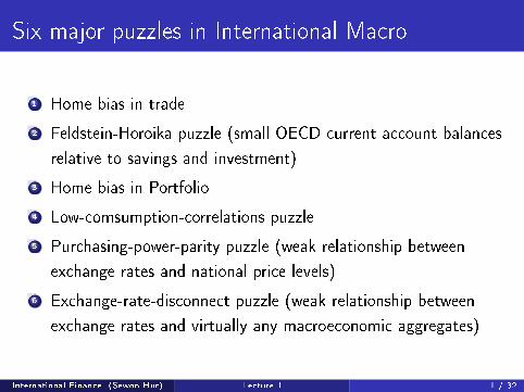
Six major puzzles in International Macro
1 Home bias in trade
2 Feldstein-Horoika puzzle (small OECD current account balances
relative to savings and investment)
3 Home bias in Portfolio
4 Low-comsumption-correlations puzzle
5 Purchasing-power-parity puzzle (weak relationship between
exchange rates and national price levels)
6 Exchange-rate-disconnect puzzle (weak relationship between
exchange rates and virtually any macroeconomic aggregates)
International Finance (Sewon Hur) Lecture 1 1 / 32
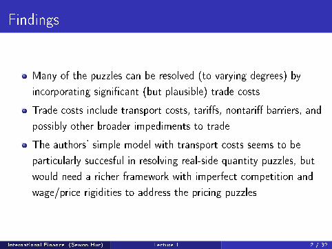
Findings
Many of the puzzles can be resolved (to varying degrees) by
incorporating signi�cant (but plausible) trade costs
Trade costs include transport costs, tari�s, nontari� barriers, and
possibly other broader impediments to trade
The authors' simple model with transport costs seems to be
particularly succesful in resolving real-side quantity puzzles, but
would need a richer framework with imperfect competition and
wage/price rigidities to address the pricing puzzles
International Finance (Sewon Hur) Lecture 1 2 / 32
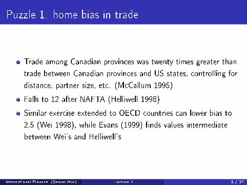
Puzzle 1: home bias in trade
Trade among Canadian provinces was twenty times greater than
trade between Canadian provinces and US states, controlling for
distance, partner size, etc. (McCallum 1995)
Falls to 12 after NAFTA (Helliwell 1998)
Similar exercise extended to OECD countries can lower bias to
2.5 (Wei 1998), while Evans (1999) �nds values intermediate
between Wei's and Helliwell's
International Finance (Sewon Hur) Lecture 1 3 / 32
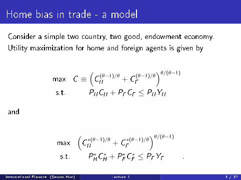
Home bias in trade - a model
Consider a simple two country, two good, endowment economy.
Utility maximization for home and foreign agents is given by
max C ≡(C
(θ−1)/θH
+ C(θ−1)/θF
)θ/(θ−1)
s.t. PHCH + PFCF ≤ PHYH
and
max(C
∗(θ−1)/θH
+ C∗(θ−1)/θF
)θ/(θ−1)
s.t. P∗HC ∗H+ P∗
FC ∗F≤ PFYF .
International Finance (Sewon Hur) Lecture 1 4 / 32
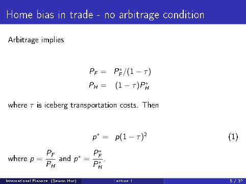
Home bias in trade - no arbitrage condition
Arbitrage implies
PF = P∗F/(1− τ)
PH = (1− τ)P∗H
where τ is iceberg transportation costs. Then
p∗ = p(1− τ)2 (1)
where p =PF
PH
and p∗ =P∗F
P∗H
.
International Finance (Sewon Hur) Lecture 1 5 / 32
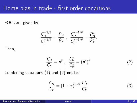
Home bias in trade - �rst order conditions
FOCs are given by
C−1/θH
C−1/θF
=PH
PF
,C
∗−1/θH
C∗−1/θF
=P∗H
P∗F
.
Then,
CH
CF
= pθ ,C ∗H
C ∗F
= (p∗)θ (2)
Combining equations (1) and (2) implies
CH
CF
= (1− τ)−2θ C∗H
C ∗F
. (3)
International Finance (Sewon Hur) Lecture 1 6 / 32

Home bias in trade
Consider the symmetric case where YH = YF . Then,CH
CF
=C ∗F
C ∗H
.
Then equation (3) reduces to
CH
CF
=C ∗F
C ∗H
= (1− τ)−θ = pθ.
Then
PHCH
PFCF
=CH
pCF
= pθ−1 = (1− τ)1−θ
and
P∗FC ∗F
P∗HC ∗H
=p∗C ∗
F
C ∗H
= pθp∗ = pθ+1(1− τ)2 = (1− τ)1−θ .
International Finance (Sewon Hur) Lecture 1 7 / 32

Home bias in trade - numerical results
If τ = 0, thenCH
pCF
= 1.
If τ = 0.25 and θ = 6, thenCH
pCF
= 4.2.
International Finance (Sewon Hur) Lecture 1 8 / 32

Home bias in trade - preferences
Now consider home bias ω < 1 in preferences
U ≡(C
(θ−1)/θH
+ ωC(θ−1)/θF
)θ/(θ−1)
and
U ≡(ωC
∗(θ−1)/θH
+ C∗(θ−1)/θF
)θ/(θ−1)
Example
Show that the e�ects of home bias in preferences (ω < 1) can be
isomorphic to the e�ects of trade costs τ .
International Finance (Sewon Hur) Lecture 1 9 / 32
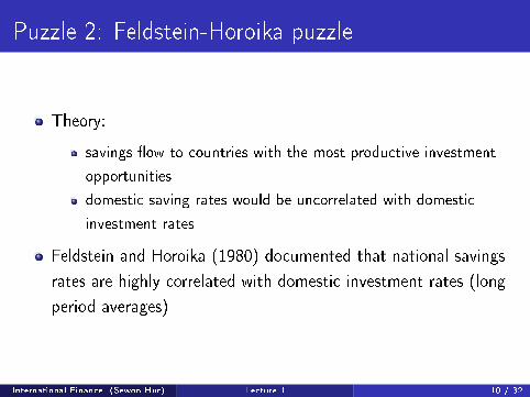
Puzzle 2: Feldstein-Horoika puzzle
Theory:
savings �ow to countries with the most productive investment
opportunities
domestic saving rates would be uncorrelated with domestic
investment rates
Feldstein and Horoika (1980) documented that national savings
rates are highly correlated with domestic investment rates (long
period averages)
International Finance (Sewon Hur) Lecture 1 10 / 32

Puzzle 2: Feldstein-Horoika puzzle
Feldstein and Horoika regressions:����� �
&��������'����(� ,����������� .//CP.//G@
�
�� �� �
#$
�� %
8�� �� %����.� � � 52
: ���������K 4A C�.4 C�5. C�11�C�C;� �C�C0�
$�������� ���� E<?7��� � .CCC 50 C�.1 C�50 C�1/�C�C;� �C�C/�
$�������� ���� E<?7��� � ;CCC 5. C�CG C�GC C�A;�C�C;� �C�C/�
"#$% ���������S ;5 C�C0 C�AC C�A0�C�C;� �C�C/�
@"D3 ������������ 3������� ������ �� ������������K����� �� ������� ��� � ����������� �� ���� ����� �� ����� �� ����� ��
��� ����� �� ���� �4A� 50� 5.�� ��� �������� �� � ��� �C�1/� C�54� C�A1��S�� ��� ���� N���� �� ��� "#$% ����� ��� ������� ��� � ����� �� C�GA�
N���� �� ������� �� ��� ����� ������
4A
International Finance (Sewon Hur) Lecture 1 11 / 32

Feldstein-Horoika puzzle - a model
Consider a two-period, two-good, small-country endowment model.
The utility function of a representative home resident is
u(C1) + δu(C2)
where
C ≡(C
(θ−1)/θH
+ C(θ−1)/θF
)θ/(θ−1)
.
International Finance (Sewon Hur) Lecture 1 12 / 32

Feldstein-Horoika puzzle - budget constraints
The small country is endowed with YH,1 in period 1, and YH,2 in
period 2. It takes as given world prices P∗H, P∗
F, r ∗. The �rst and
second period budget constraints are given by
PH,1CH,1 + PF ,1CF ,1 ≤ PH,1YH,1 + D
PH,2CH,2 + PF ,2CF ,2 ≤ PH,2YH,2 − (1+ r ∗) D
International Finance (Sewon Hur) Lecture 1 13 / 32

Feldstein-Horoika puzzle - �rst order conditions
FOCs are given by
(CH,1)−1/θ
C 1/θ = PH,1λ1 (4)
(CF ,1)−1/θ
C 1/θ = PF ,1λ1 (5)
International Finance (Sewon Hur) Lecture 1 14 / 32

Feldstein-Horoika puzzle
Combine equations (4) and (5),
(C
(θ−1)/θH,1 + C
(θ−1)/θF ,1
)C (1−θ)/θ =
(P1−θH,1 + P1−θ
F ,1
)λ1−θ1(
C(θ−1)/θH,1 + C
(θ−1)/θF ,1
)θ/(θ−1)
C−1 =(P1−θH,1 + P1−θ
F ,1
)θ/(θ−1)λ−θ1
λ1 = P−1
1
where
P1 =(P1−θH,1 + P1−θ
F ,1
)1/(1−θ)(6)
International Finance (Sewon Hur) Lecture 1 15 / 32

Feldstein-Horoika puzzle
Therefore the consumption of home and foreign goods are
CH,t =
(PH,t
Pt
)−θ
Ct , CF ,t =
(PF ,t
Pt
)−θ
Ct t = 1, 2 (7)
The �rst period budget constraint can be written as
PH,1CH,1 + PF ,1CF ,1 = P1−θH,1 P
θ1C1 + P1−θ
F ,1 Pθ1C1
=(P1−θH,1 + P1−θ
F ,1
)Pθ
1C1
= P1C1
≤ PH,1YH,1 + D
International Finance (Sewon Hur) Lecture 1 16 / 32

Feldstein-Horoika puzzle
Similarly, the second period budget constraint is
P2C2 ≤ PH,2YH,2 − (1+ r ∗)D
Combining the budget constraints,
P1C1 +P2C2
1+ r ∗= PH,1YH,1 +
PH,2YH,2
1+ r ∗.
International Finance (Sewon Hur) Lecture 1 17 / 32

Feldstein-Horoika puzzle
Let the domestic real interest rate be de�ned as
1+ r = (1+ r ∗)P1/P2, (8)
Then the consolidated intertemporal budget constraint is
C1 +C2
1+ r=
PH,1
P1
YH,1 +PH,2
P2
YH,2
1+ r.
Given P1 and P2, equation (8) determines the real interest rate faced
by domestic agent.
International Finance (Sewon Hur) Lecture 1 18 / 32
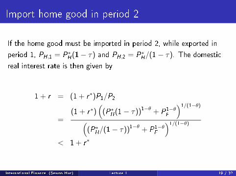
Import home good in period 2
If the home good must be imported in period 2, while exported in
period 1, PH,1 = P∗H(1− τ) and PH,2 = P∗
H/(1− τ). The domestic
real interest rate is then given by
1+ r = (1+ r ∗)P1/P2
=(1+ r ∗)
((P∗
H(1− τ))1−θ + P1−θ
F
)1/(1−θ)
((P∗
H/(1− τ))1−θ + P1−θ
F
)1/(1−θ)
< 1+ r ∗
International Finance (Sewon Hur) Lecture 1 19 / 32
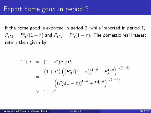
Export home good in period 2
If the home good is exported in period 2, while imported in period 1,
PH,1 = P∗H/(1− τ) and PH,2 = P∗
H(1− τ). The domestic real interest
rate is then given by
1+ r = (1+ r ∗)P1/P2
=(1+ r ∗)
((P∗
H/(1− τ))1−θ + P1−θ
F
)1/(1−θ)
((P∗
H(1− τ))1−θ + P1−θ
F
)1/(1−θ)
> 1+ r ∗
International Finance (Sewon Hur) Lecture 1 20 / 32
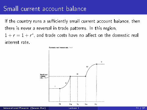
Small current account balance
If the country runs a su�ciently small current account balance, then
there is never a reversal in trade patterns. In this region,
1+ r = 1+ r ∗, and trade costs have no a�ect on the domestic real
interest rate.
354 * OBSTFELD & ROGOFF
Figure 1 DOMESTIC SPENDING AND THE DOMESTIC REAL INTEREST RATE IN A TWO-GOOD MODEL WITH TRADE COSTS
Domestic real interest rate, 1 + r
V
World real l / interest -------- -- rate, 1 + r
First-period total real spending, Cl
CH,2 > YH,2 Since in period 2 the home good must be imported, while in
period 1 it is exported, we have
(1 + r*) (P,-19 + P- 9)11(1-9) 1 +
H F (Pk2 ? P:/9)
(1 + r*) {[PH(1 - 7)11-0 + Pl-}1/(1- ) F= < 1 + r*
{[P/(1 -
T)]1- + p/-F 1/-(0)
in segment I. If the country contemplates being a big lender, it will face an effective real interest rate significantly below the world real interest rate.
Segment II starts when period 1 consumption first reaches the level Cln such that CH,2 = YH,2- In this region, PH,2 is determined by equation (8) and the first relation in equation (9), with CH,2
= YH,2 (so there is no round-
International Finance (Sewon Hur) Lecture 1 21 / 32
Numerical Example
If r ∗ = 0.05, τ = 0.1, θ = 0.6, P∗H= P∗
F= 1, the highest
possible real interest rate is 20 percent, while the lowest is -8
percent
This can put a check on a country's incentives to run large
current account de�cits or surpluses (and thus large
savings-investment di�erentials)
International Finance (Sewon Hur) Lecture 1 22 / 32
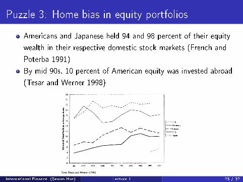
Puzzle 3: Home bias in equity portfolios
Americans and Japanese held 94 and 98 percent of their equity
wealth in their respective domestic stock markets (French and
Poterba 1991)
By mid 90s, 10 percent of American equity was invested abroad
(Tesar and Werner 1998)360 * OBSTFELD & ROGOFF
Figure 2 HOME BIAS IN EQUITY PORTFOLIOS: 1987-1996
26
24
22 , ,
. 16 |;~~~~~~~ 16 -\-----
- l- - - I. K
.S 14 (-Germany
| f10 2^^ y^^"^^"*- - " -Canada
l 12
l f ~----- Japan
X l.
4
1987 1988 1989 990 1991 2 13 1994 15 1996 1987 1988 1989 1990 1991 1992 1993 1994 1995 1996
From Tesar and Werner (1998)
Potential explanations range from nontraded factors such as human
capital (which may worsen or reduce the puzzle; see Baxter and Jermann, 1997) to nontraded consumption goods to asymmetries of information to data inadequacy. Yet it is fair to say that none of the available stories alone has provided a quantitatively satisfactory account of the observed home bias; see Lewis (1999) for an up-to-date and thorough survey.
To set the stage for our discussion of trade costs, it is worthwhile
briefly reviewing what is perhaps the leading explanation, which is based on the classic Salter-Swan traded-nontraded-goods dichotomy we have already mentioned. While these two types of goods lie at polar extremes in terms of their tradability, equity claims on either type of
industry can be frictionlessly traded. Thus, even though cement is
prohibitively costly to transport, there is nothing to stop foreign inves- tors from buying shares in the domestic cement industry. Earnings, of course, must be redeemed in traded goods, since nontradables cannot be shipped to foreign equity holders by assumption. The key result one
gets out of this framework is that, for the baseline case of separable
to 7%. The positive target position in foreign equities, meant to "reduce risk and broaden portfolio diversification while maintaining or improving investment perfor- mance," represents a substantial advance. It still falls far short, however, of the optimal foreign equity share that simple models of international diversification would predict.
International Finance (Sewon Hur) Lecture 1 23 / 32
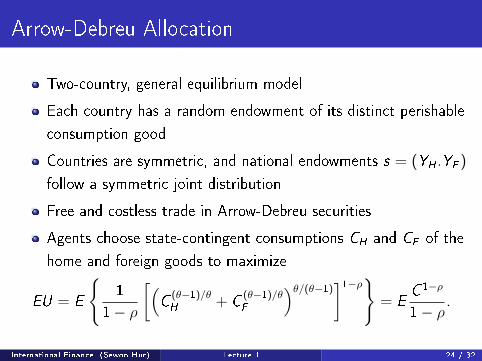
Arrow-Debreu Allocation
Two-country, general equilibrium model
Each country has a random endowment of its distinct perishable
consumption good
Countries are symmetric, and national endowments s = (YH .YF )
follow a symmetric joint distribution
Free and costless trade in Arrow-Debreu securities
Agents choose state-contingent consumptions CH and CF of the
home and foreign goods to maximize
EU = E
{1
1− ρ
[(C
(θ−1)/θH
+ C(θ−1)/θF
)θ/(θ−1)]1−ρ}
= EC 1−ρ
1− ρ.
International Finance (Sewon Hur) Lecture 1 24 / 32
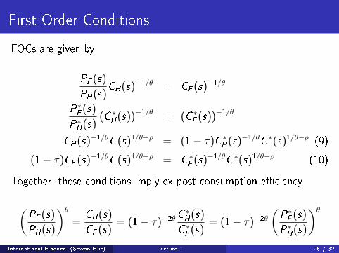
First Order Conditions
FOCs are given by
PF (s)
PH(s)CH(s)
−1/θ = CF (s)−1/θ
P∗F(s)
P∗H(s)
(C ∗H(s))−1/θ = (C ∗
F(s))−1/θ
CH(s)−1/θC (s)1/θ−ρ = (1− τ)C ∗
H(s)−1/θC ∗(s)1/θ−ρ (9)
(1− τ)CF (s)−1/θC (s)1/θ−ρ = C ∗
F(s)−1/θC ∗(s)1/θ−ρ (10)
Together, these conditions imply ex post consumption e�ciency
(PF (s)
PH(s)
)θ=
CH(s)
CF (s)= (1− τ)−2θC
∗H(s)
C ∗F(s)
= (1− τ)−2θ
(P∗F(s)
P∗H(s)
)θInternational Finance (Sewon Hur) Lecture 1 25 / 32

Arrow-Debreu Allocation
The model is closed by the output-market clearing conditions:
C ∗H(s) = (1− τ) (YH(s)− CH(s)) (11)
CF (s) = (1− τ) (YF (s)− C ∗F(s)) (12)
We have four equations, (9)-(12), and four unknowns,
CH ,CF ,C∗H,C ∗
Ffor every state s.
International Finance (Sewon Hur) Lecture 1 26 / 32

Arrow-Debreu Allocation
Assume that ρ = 1/θ. Then
CH(s) =1
1+ (1− τ)θ−1YH(s)
CF (s) =(1− τ)θ
1+ (1− τ)θ−1YF (s)
Equity shares are given by
XH =1
1+ (1− τ)θ−1YH
XF =(1− τ)θ−1
1+ (1− τ)θ−1YF
International Finance (Sewon Hur) Lecture 1 27 / 32
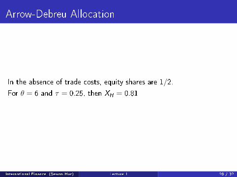
Arrow-Debreu Allocation
In the absence of trade costs, equity shares are 1/2.
For θ = 6 and τ = 0.25, then XH = 0.81
International Finance (Sewon Hur) Lecture 1 28 / 32

Equity Trade Allocation
Now consider the model without Arrow-Debreu securities, but with
trade in equity shares to each country's output.
Example
Assume that ρ = 1/θ. Show that the equity trade allocation is
identical to the Arrow-Debreu allocation.
International Finance (Sewon Hur) Lecture 1 29 / 32
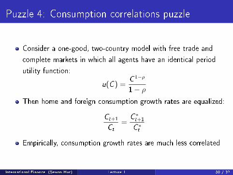
Puzzle 4: Consumption correlations puzzle
Consider a one-good, two-country model with free trade and
complete markets in which all agents have an identical period
utility function:
u(C ) =C 1−ρ
1− ρ
Then home and foreign consumption growth rates are equalized:
Ct+1
Ct
=C ∗t+1
C ∗t
Empirically, consumption growth rates are much less correlated
International Finance (Sewon Hur) Lecture 1 30 / 32

Puzzle 5: Purchasing-power-parity puzzle
Let Q be the real exchange rate between two countries
Q = eP∗
P
where e is the nominal exchange rate
Consider the regression:
logQt = α + ηt + γ logQt−1 + εt
γ ranges from 0.99 (US-Canada; half-life of 69 months) to 0.97
(Germany-Japan; 21 months)
Half-lives of this magnitude are hard to understand if
�nancial-market disturbances with only transitory real e�ects are
very important in explaining short-run volatility.
International Finance (Sewon Hur) Lecture 1 31 / 32
Puzzle 6: Exchange rate disconnect puzzle
Remarkably weak short-term feedback links between exchange
rate and the rest of the economy
PPP puzzle is a special case
Similar to stock-price disconnect puzzle, but links between
exchange rate and real economy are much more direct than for
stock prices
A model with imperfect markets, trade costs, and nominal
rigidities can produce a disconnect in which the exchange rate
responds wildly to shocks
International Finance (Sewon Hur) Lecture 1 32 / 32