The Simulation of Large Industrial Centrifugal Compressors.

Louisiana State UniversityLSU Digital Commons

LSU Historical Dissertations and Theses Graduate School

1972

The Simulation of Large Industrial CentrifugalCompressors.Frank Tate DavisLouisiana State University and Agricultural & Mechanical College

Follow this and additional works at: https://digitalcommons.lsu.edu/gradschool_disstheses

This Dissertation is brought to you for free and open access by the Graduate School at LSU Digital Commons. It has been accepted for inclusion inLSU Historical Dissertations and Theses by an authorized administrator of LSU Digital Commons. For more information, please [email protected].

Recommended CitationDavis, Frank Tate, "The Simulation of Large Industrial Centrifugal Compressors." (1972). LSU Historical Dissertations and Theses.2334.https://digitalcommons.lsu.edu/gradschool_disstheses/2334

https://digitalcommons.lsu.edu?utm_source=digitalcommons.lsu.edu%2Fgradschool_disstheses%2F2334&utm_medium=PDF&utm_campaign=PDFCoverPages

https://digitalcommons.lsu.edu/gradschool_disstheses?utm_source=digitalcommons.lsu.edu%2Fgradschool_disstheses%2F2334&utm_medium=PDF&utm_campaign=PDFCoverPages

https://digitalcommons.lsu.edu/gradschool?utm_source=digitalcommons.lsu.edu%2Fgradschool_disstheses%2F2334&utm_medium=PDF&utm_campaign=PDFCoverPages

https://digitalcommons.lsu.edu/gradschool_disstheses?utm_source=digitalcommons.lsu.edu%2Fgradschool_disstheses%2F2334&utm_medium=PDF&utm_campaign=PDFCoverPages

https://digitalcommons.lsu.edu/gradschool_disstheses/2334?utm_source=digitalcommons.lsu.edu%2Fgradschool_disstheses%2F2334&utm_medium=PDF&utm_campaign=PDFCoverPages

mailto:[email protected]

INFORMATION TO USERS

This dissertation was produced from a microfilm copy of the original document. While the most advanced technological means to photograph and reproduce this document have been used, the quality is heavily dependent upon the quality of the original submitted.

The following explanation of techniques is provided to help you understand markings or patterns which may appear on this reproduction.

1. The sign or "target" for pages apparently lacking from the document photographed is "Missing Page(s)". If it was possible to obtain the missing page(s) or section, they are spliced into the film along with adjacent pages. This may have necessitated cutting thru an image and duplicating adjacent pages to insure you complete continuity.

2. When an image on the film is obliterated with a large round black mark, it is an indication that the photographer suspected that the copy may have moved during exposure and thus cause a blurred image. You will find a good image of the page in the adjacent frame.

3. When a map, drawing or chart, etc., was part of the material being photographed the photographer followed a definite method in "sectioning" the material. It is customary to begin photoing at the upper left hand corner of a large sheet and to continue photoing from left to right in equal sections with a small overlap. If necessary, sectioning is continued again — beginning below the first row and continuing on until complete.

4. The majority of users indicate that the textual content is of greatest value, however, a somewhat higher quality reproduction could be made from "photographs" if essential to the understanding of the dissertation. Silver prints of "photographs" may be ordered at additional charge by writing the Order Department, giving the catalog number, title, author and specific pages you wish reproduced.

University Microfilms300 North Zeeb RoadAnn Arbor, Michigan 48106

A Xerox Education Company

73- 13,658

DAVIS, frank Tate, 1942~.THE SIMULATION OF LARGE INDUSTRIAL CENTRIFUGAL COMPRESSORS.

The Louisiana State University and Agricultural and Mechanical College, Ph.D., 1972 Engineering, chemical

University Microfilms, A XEROX Company, Ann Arbor. Michigan

© 1973FRANK TATR DAVIS

ALL RIGHTS RESERVED

THE SIMULATION OF

LARGE INDUSTRIAL CENTRIFUGAL COMPRESSORS

A Dissertation

Submitted to the Graduate Faculty of the Louisiana State University and

Agricultural and Mechanical College in partial fulfillment of the requirements for the degree of

Doctor of Philosophy

in

The Department of Chemical Engineering

byFrank Tate Davis

B.S., Auburn University, 1968 M.S., Auburn University, 1969

December 1972

PLEASE NOTE:

Some pages may have

indistinct print. Filmed as received.

University Microfilms, A Xerox Education Company

This work Is dedicated to

the memory of my late father,

Sam Tate Davis, Jr.

ACKNOWLEDGEMENT

This research was conducted under the guidance of Dr. A. B.

Corriplo, Assistant Professor of the Department of Chemical Engineer

ing, The author is highly appreciative of the assistance given by

Dr. Corrlpio during this study.

The author wishes to express his appreciation for the support

of this work by Project THEMIS, Contract Number F-44620-68-C-0021,

administered for the U.S. Department of Defense by the U.S. Air

Force Office of Scientific Research. Without this support the

author's research would have been financially impossible.

The author also wishes to thank the General Electric Company,

in particular Mr. W. I. Rowen, Supervisor, Control Systems Analysis,

for the time and effort spent in answering questions pertaining to

this reaserch and for providing copies of several pertinent research

papers. Further thanks are extended to Mr. W. C. Cutter, Sales

Engineer for General Electric, for making available the papers con

tained within the General Electric Gas Turbine Library and for pro

viding design data of a steam turbine centrifugal compressor

installation.*

Thanks are extended also to the Worthington Corporation, Mr.

L. M. Anderson, Control Engineer, for providing design parameters

of several steam turbine Installations.

Clark Brothers, a Division of Dresser Industries, Inc. provided,

through Mr. J. R. Lewis, Local Sales Engineer, the design parameters

ii

of several centrifugal compressor installations for the author's study.

Mr. Lewis spent much time answering questions dealing with the compres

sors, via letters and telephone conversations, and for the this the

author is grateful.Cooper-Bessemer Company's local Sales Engineer, Mr. Frank P. Sims,

made available design characteristics of several centrifugal compressors and graciously answered numerous questions on the subject material.

Particular thanks are extended to Mr. R. E. Ruckstuhl of Enjay Chemical Company for making available the design parameters of a centrifugal compressor and steam turbine installation.

Thanks are also due to the following people who provided technical

Information and encouragement in the author's research: Woodward Governor Company, Mr. George E. Parker; Crawford and Russell Incorporated, Mr. F. B. Horowitz; Shell Development Company, Dr. S. A. Shain; and the Foxboro Company, Mr. T. L. Magliozzi.

Too, the author wishes to express appreciation to the computer operators of the Computer Research Center of Louisiana State University

and especially to the workers who operated the Calcomp Plotter for their patience in producing plots repeatedly in order to obtain exacting results. Deep appreciation is extended to Mr. James A. Paulsen, Associate, Chemical Engineering Department, for his continued efforts in assisting the author in writing and debugging the simulation programs.

The author wishes to thank the Dr. Charles E. Coates Memorial Fund, donated by George H. Coates, for financial assistance in the preparation of this manuscript.

Finally, a special thanks Is expressed to the author's wife, Mona, for her unending encouragement and for her assistance In the typing of this manuscript.

iii

TABLE OF CONTENTSPage

ACKNOWLEDGMENT................................................. ii

LIST OF TABLES.................................. vll

LIST OF F I G U R E S ................................................. viii

ABSTRACT ..................................................... xiv

CHAPTERI INTRODUCTION ...................................... 1

Literature Cited .................................. 7

II THE CONSTANT SPEED IDEAL GAS MODEL (CSIGM) . . . . 8

Introduction..................... . 8

The Physical System ............................. 9

Mathematical Model ............................. 11

Suction System . . . . . ......................... 11

Discharge S y s t e m .................................. 18

Compressor.......... .............................. 20

Integration Method ............................. 32

Open-Loop Responses ............................. 33

Closing the L o o p .................................. 42

Dynamics of the Control Valve andTransmission Line . . . . . . . . . . . .......... 43

The Controller....................... 46

Closed Loop Responses.............. . .. 52

Summary .......................................... 63

Nomenclature ...................................... 65

Literature Cited .................................. 68

iv

PageIII THE CONSTANT SPEED REAL GAS MODEL (CSRGM)............ 70

Introduction....................................... . 70

Mathematical Model . . . . . 72

Suction System ...................................... 72

Discharge System . . . . . .......................... 77

Compressor.......................................... 77

Open-Loop Responses .................................. 89

Closed-Loop Results .................................. 97

Summary............................................... 113

Nomenclature ........................................ 115

Literature Cited .................................... 118

IV THE VARIABLE SPEED MODELS............................ 119

Introduction ........................................ 119

The P l a n t ............................................. 122

Correlating the Variable Speed Performance Map . . . 124

Converting the Constant Speed Models toVariable Speed Models .............................. 150

The Steam Turbine Model .................. 150

The Open Loop Responses.............................. 158

Summary............................................... 180

Nomenclature . . . . . . . 182

Literature Cited .................................... 184

V CONCLUSIONS AND RECOMMENDATIONS ...................... 186

APPENDIX

A STEADY STATE DESIGN OF THE PLANT .................... 189

B IMPLICIT LOOP SOLVING ROUTINES ...................... 196

v

PageC PROCESS REACTION CURVES ............................... 204

D THERMODYNAMIC DERIVATIONS ............................. 221

E CSMP COMPUTER PROGRAM OF THE VSRGM AND THE VSIGM . . . 231

F COMPUTER PROGRAM FOR CORRELATING THE VARIABLE SPEEDPERFORMANCE CURVES .................................... 243

V I T A ...............................................................253

vl

LIST OF TABLES

Table Page

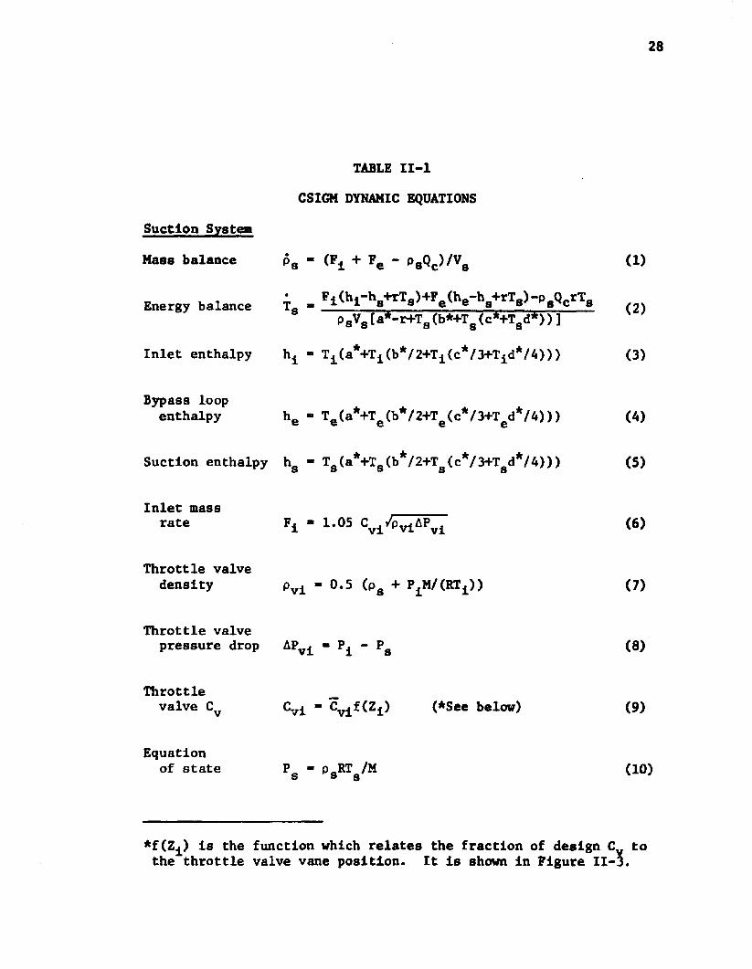
II-l CSIGM Dynamic Equations............. 28

II-2 Open-Loop Results for Inlet PressureChanges (CSIGM)..................................... 39

II-3 Open-Loop Results for Inlet TemperatureChanges (CSIGM)............................... 39

II-4 Open-Loop Results for Molecular WeightChanges (CSIGM) ...................................... 39

II-5 Open-Loop Results for Load Demand Changes (CSIGM) . . 43

II-6 Process Reaction Curve Results (CSIGM) ............. 48

II-7 Optimization Results (CSIGM) ...................... . 62

III-l CSRGM Dynamic Equations ........................ . . . 82

III-2 Open-Loop Comparison of CSRGM with C S I G M ..........94

III-3 Process Reaction Curve Results ...................... 99

III-4 Closed Loop CSRGM Optimization R e s u l t s ............. 112

IV-1 Compressor Characteristics and CorrelationResults.............................................132

vii

LIST OF FIGURES

Figure Page

II-l The Constant Speed P l a n t ................. 10

II-2 The Lumped Parameter Model .......................... 12

II-3 Characteristics of Butterfly Valves ............... 14

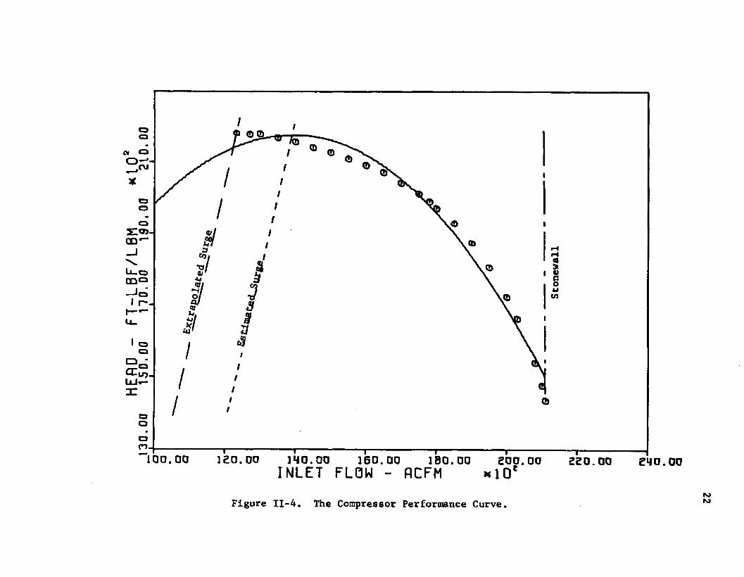
II-4 The Compressor Performance Curve .................... 22

II-5 Information Flow Diagram forOpen Loop C S I G M .................................. 27

II-6 Open Loop Time Response of Discharge Pressureto Step Changes in Inlet P r e s s u r e ............... 34

II-7 Open Loop Time Response of Discharge Pressureto Step Changes in Inlet Temperature for for Both the Simplified and the Ideal Suction System Energy Balances ................. 35

II-8 Open Loop Time Response of Discharge Pressureto Step Changes in Molecular Weight . ........ 36

II-9 Open Loop Time Response of Discharge Pressureto Step Changes in the Demand Load R a t e ........ 37

11-10 The Closed Loop System . 44

11-11 Determination of the Process Gain K Basedon the CSIGM .................................... 49

11-12 Determination of the Process Time Constant t

Based on the CSIGM .............................. 50

11-13 Determination of the Process Dead-Time 0,Based on the CSIGM ........ . ................... 50

11-14 Closed Loop Response to 5% Decrease inthe Demand Load R a t e « . . . 54

11-15 Closed Loop Response to 5% Increase in theDemand Load Rate F ................... 55o

11-16 Closed Loop Response to 5 psl Step Change inSet-Polnt for the C S I G M ........................ . 56

vlil

58

59

60

61

81

90

91

92

93

100

101

101

104

105

106

107

Closed Loop Response to -5 psi Step ChangeIn Set-Point for the C S I G M ................ . . .

Closed Loop Response to 5 psl Step Changein Inlet Pressure for the C S I G M .......... . . .

Closed Loop Response to -10°F Step Change InInlet Temperature for the CSIGM .................

Closed Loop Response to 10°F Step Change InInlet Temperature for the C S I G M .................

Closed Loop Response to 3 lbm/mole StepChange in Molecular Weight for the CSIGM ........

Information Flow Diagram for Open Loop CSRGM ♦ . . .

Open Loop Response of the CSRGM to StepChanges in Inlet Pressure .......................

Open Loop Response of the CSRGM to Step Changes in Inlet Temperature for (1) the Simplified,(2) the Ideal and (3) the Real SuctionEnergy Balances ..................................

Open Loop Response of the CSRGM to Step Changes inMolecular Weight of the Gas .....................

Open Loop Response of the CSRGM to Step Changesin the Load Demand Rate .........................

Determination of the Process Gain Based onthe C S R G M . . .

Determination of the Process Time ConstantBased on the CSRGM ................................

Determination of the Process Dead Time Basedon the CSRGM ......................................

Closed Loop Response of the CSRGM to 5% Decrease in Load Demand Rate ..............................

Closed Loop Response of the CSRGM to 5% Increase in Load Demand Rate ..............................

Closed Loop Response of the CSRGM to 5 psi Step Change in Set-Point ..............................

Closed Loop Response of the CSRGM to -5 psiStep Change in Set-Point .........................

ix

13 Closed Loop Response of the CSRGM to 5 pel

Step Change In Inlet Pressure.......................108

111-14 Closed Loop Response of the CSRGM to -2 psiStep Change In Inlet Pressure ............ 109

111-15 Closed Loop Response of the CSRGM to -10°F StepChange in Inlet Temperature ..................... 110

111-16 Closed Loop Response of the CSRGM to 10°F StepChange In Inlet Temperature ..................... Ill

IV-1 The Variable Speed P l a n t ..............................123

IV-2 The Variable Speed Compressor Performance MapUsed in the VSIGM and V S R G M ......................... 126

IV-3 Computer Flow Diagram of the Correlation Procedure . 130

IV-4 Reduced Performance Curve of Compressor Usedin the VSIGM and V S R G M ............................. 131

IV-5A Reduced Performance Curve of the 1900 HorsepowerCentrifugal Compressor ........................... 133

IV-5B Variable Speed Performance Map of a 1900Horsepower Centrifugal Compressor ................. 134

IV-6A Reduced Performance Curve of the 2200 HorsepowerCentrifugal Compressor ............................ 135

IV-6B Variable Speed Performance Map of a 2200 HorsepowerCentrifugal Compressor ............................ 136

IV-7A Reduced Performance Curve of the 3100 HorsepowerCentrifugal Compressor with the Speed Range of 3400-5100 R P M ................................... 137

IV-7B Variable Speed Performance Map of a 3100Horsepower Centrifugal Compressor with theSpeed Range of 3400-5100 RPM ................ . 138

IV-8A Reduced Performance Curve of the 3100 HorsepowerCentrifugal Compressor with the Speed Range of 8000-9400 R P M ................................... 139

IV-8B Variable Speed Performance Map of a 3100Horsepower Centrifugal Compressor with theSpeed Range of 8000-9400 RPM......................... 140

x

PageIV-9A Reduced Performance Curve of the 4300

Horsepower Centrifugal Compressor ................. 141


IV-10A Reduced Performance Curve of the 5000Horsepower Centrifugal Compressor . ............... 143






IV-13 The Steam Turbine...................................... 151

IV-14 Performance Characteristics of the Steam Turbine . . 153

IV-15 Governor Valve Flow Characteristics ................. 156

IV-16 The Steam Turbine M o d e l ................................157

IV-17 VSRGM and VSIGM Open-Loop Discharge PressureResponses for Step Increases in the Inlet P r e s s u r e ............................................159

IV-18 VSRGM and VSIGM Open-Loop Speed Responses forStep Increases In the Inlet P r e s s u r e .............. 160

IV-19 VSRGM and VSIGM Open-Loop Discharge PressureResponses for Step Decreases in the Inlet P r e s s u r e ............................................161

IV-20 VSRGM and VSIGM Open-Loop Speed Responses forStep Decreases in the Inlet Pressure . . . . . . . 162

IV-21 VSRGM and VSIGM Open-Loop Discharge PressureResponses for Step Increases in the Inlet Temperature ........................“............ .163

IV-22 VSRGM and VSIGM Open-Loop Speed Responsesfor Step Increases in the Inlet Temperature . . . . 164

xl

PageIV-23 VSRGM and VSIGM Open-Loop Discharge Pressure

Responses for Step Decreases in the Inlet Temperature.......................................... 165

IV-24 VSRGM and VSIGM Open-Loop Speed Responses forStep Decreases in the Inlet Temperature............. 166

IV-25 VSRGM and VSIGM Open-Loop Discharge PressureResponses for Step Increases in Molecular Height . 167

IV-26 VSRGM and VSIGM Open-Loop Speed Responsesfor Step Increases in Molecular W e i g h t .............168

IV-27 VSRGM and VSIGM Open-Loop Discharge Pressure Responsesfor Step Decreases in Molecular Height . . . . . . 169

IV-28 VSRGM and VSIGM Open-Loop Speed Responses forStep Decreases in Molecular Weight .............. 170

IV-29 VSRGM and VSIGM Open-Loop Discharge PressureResponses for Step Increases in the Load Demand R a t e ..........................................172

IV-30 VSRGM and VSIGM Open-Loop Speed Responses forStep Increases in the Load Demand R a t e .............173

IV-31 VSRGM and VSIGM Open-Loop Discharge PressureResponses for Step Decreases in the Load Demand R a t e ..........................................174

IV-32 VSRGM and VSIGM Open-Loop Speed Responses forStep Decreases in the Load Demand R a t e .............175

IV-33 VSRGM and VSIGM Open-Loop Discharge PressureResponses for Step Increases in the GovernorO u t p u t .............................................. 176

IV-34 VSRGM and VSIGM Open-Loop Speed Responses forStep Increases in the Governor Output............... 177

IV-35 VSRGM and VSIGM Open-Loop Discharge PressureResponses for Step Decreases in the GovernorO u t p u t .............................................. 178

IV-36 VSRGM and VSIGM Open-Loop Speed Responses forStep Decreases in the Governor Output............... 179

B-l Computer Flow Diagram for Newton's MethodFor Solving Implicit Functions . . . . . . . . . . 198

xii

PageB-2 Trial and Error Procedure for the

Inlet Density........................................203

C-l CSIGM Process Reaction Curve for 1.4 psiStep Change in Controller Output ................. 205

C-2 CSIGM Process Reaction Curve for 1. psiStep Change In Controller Output ................ 206

C-3 CSIGM Process Reaction Curve for 0.5 psi StepChange in Controller Output ........................ 207

C-4 CSIGM Process Reaction Curve for 0.25 psi StepChange in Controller Output ........................ 208

C-5 CSIGM Process Reaction Curve for -0.25 psi StepChange in Controller Output ........................ 209




C-9 CSRGM Process Reaction Curve for 1.4 psi StepChange in Controller Output ........................ 213


C-ll CSRGM Process Reaction Curve for 0.5 psi StepChange in Controller Output ........................ 215


C-13 CSRGM Process Reaction Curve for -0.25 psi StepChange in Controller Output ........................ 217




xili

ABSTRACT

This research effort presents the detailed development of dynast

1c models of the constant and variable speed centrifugal compressors.

In conjunction with the variable speed model, a model of the steam

turbine Is developed. Each model is of the lumped parameter type

and the compressor models are capable of handling any real gas or

mixture of real gases for which an equation of state is known. Each

model was developed so that no data other than that ordinarily sup

plied to the plant personnel by the compressor and turbine manufac

turers is required. Use was made of the performance characteristics

of a compressor and turbine which are in operation today. The re

sulting models were implemented on an IBM 360/65 digital computer

utilizing CSMP and on an XDS 15 digital computer utilizing SL1.

The initial compressor model is based on the ideal gas equation

of state and is called the constant speed ideal gas model (CSIGM).

Open loop responses of the discharge pressure are given for step

changes in the inlet temperature and pressure, the molecular weight

of the gas and the mass rate demanded by the downstream unit. These

responses are given in terms of continuous curves. The discharge

pressure control loop was closed with a pneumatic controller. The

dynamics of the control valve were included. The controller was

tuned based on a first order lag with dead time model and based on

the CSIGM. Closed loop results are given for each controller

xiv

indicating the discharge pressure responses to the above disturbances

as well as changes in the discharge pressure set point.

The CSIGM was then extended so as to account for the nonideali

ties of the gas through the incorporation of a modified Benedict-

Webb-Rubin equation of state into the model. Open and closed loop

simulation results paralleling those of the CSIGM are given. The

responses of the real gas model are compared to those of the CSIGM

and the additional computer time and storage requirements along with

the increased difficulty of programming the real gas model are

pointed out.

Finally, modifications are presented which convert the constant

speed models to variable speed models. The modifications center

around a unique correlation of the compressor performance map in

which the several head curves are made to collapse into one curve

which can be adequately represented by a simple parabolic equation.

The correlation is tested for nine compressors ranging in size from

1900 to 8600 brake horsepower and in speed from 3000 to 10000 rpm.

Open loop responses of the discharge pressure of the compressor and

the speed of the steam turbine are given for the ideal and the real

gas variable speed models. The responses are for step changes in

the above mentioned compressor variables in addition to step changes

in the steam turbine governor output. A comparison is made of the

responses produced by each model.

xv

CHAPTER I

INTRODUCTION

The number of applications of digital computers in process

control has Increased in the past few years. Concurrently, the

theory of advanced control concepts such as feedforward, adaptive,

predictive, multivariable and optimal control have been developed

and/or refined. Even though the digital computer is ideally suited

for implementation of control strategies based on these concepts,

which is the major advantage the digital controller has over the

analog controller, the digital computer has been used in most

cases merely as a substitute for the conventional analog controller.

The major reason is that control strategies based on the advanced

control concepts cannot be readily developed without a mathematical

model of the process.

At the inception of chemical engineering it was postulated

that most processes are made up of a number of operations that are

similar enough to be studied by themselves, independent of the type

of process of which they are a part. These were called "unit opera

tions" and the graduates trained in their design and study were

called "chemical engineers." Since each of the unit operations in a

process is controlled independently of the others it appears that it

would be prudent on the part of chemical engineers to follow the path

of the founding fathers and develop mathematical models of each unit

operation. With the mathematical models the capabilities and

2

flexibilities of the digital computer could then be realized

through the application of the advanced concepts.

Scarcely a plant in the chemical process industries lacks at

least an air compressor for supply of plant air. In many plants

reciprocating, centrifugal and axial compressors serve as process

equipment to help bring about reactions and phase separations, or

to provide refrigeration. Many plants use them in materials handling,

in liquefying or storing gases, in agitation, in lifting fluids

from wells or moving them in pipes. Most plant shops use them to

power air tools and, in processes with explosion hazards, they often

drive air motors on agitators and other mechanical equipment.

Utilization of centrifugal compressors has become more prevalent

in industry today because plant capacities have Increased and because

installation costs for centrifugals are lower and operating costs are

less. Such units are being used in many applications. Typical of

some of these are: air for blast furnaces, Bessemer converters and

wind tunnels. Within the process industries they have found use in

chemical processes such as nitric and sulfuric acid, synthesis of

ammonia and methanol, and in refrigeration cycles handling ammonia,

Freon-11 and hydrocarbon gases. Refineries have found many uses for

centrifugal compressors in vapor recovery, catalytic reforming, cata

lytic cracking and ethylene and butadiene plants. In some processes,

particularly the high-pressure industries such as ammonia and poly

ethylene, the compressor accounts for a sizeable part of the plant's

capital cost.

Because the centrifugal compressor is a dynamic machine, its

performance characteristics are such that unless adequate and proper

3

control Is provided, through Instrumentation, the compressor loop

may become unstable, causing costly surging and upsets in the com

pressor and process. In order to more readily develop the ade

quate and proper control strategies to prevent these upsets, the

control engineer requires a dynamic model of the centrifugal

compressor, one that might be easily implemented on either an

analog, digital, or hybrid computer. For without the computer

model, it would be almost impossible to ascertain the validity

of a proposed control scheme because in a dynamic analysis of

the centrifugal compressor too many variables come into play.

An exhaustive literature search has revealed only three

papers which present dynamic models of centrifugal compressors

and each of these appeared in 1971. The paper by Nlsenfeld and

co-workers [1] does not present enough detail for a complete analy

sis of their model but it appears that it is limited in scope.

The paper by Jeffrey [2] presents a detailed development of a dyna

mic model of a variable speed centrifugal air compressor in the

form of an analog diagram. The appendix giving the development

of the dynamic equations was omitted from the publication. The

major disadvantage of his model is that it depends upon extensive

in-plant testing. The paper by Bergeron and Corripio [3] also

presents a detailed development in the form of an analog diagram of

the dynamic model of a multistage centrifugal compressor used in

a refrigeration system. The major drawback of their model is that

it is valid only for a pure component feed gas as it depends upon

thermodynamic data in the form of a MolHer diagram. Much detail

was omitted because of the restricted nature of the plant data.

4

Their analog model does present a novel way in which to simulate the

surge of the compressor.

These several citations of need have provided the Impetus for

this research effort which involves the development of dynamic

models of the constant speed centrifugal compressor and the variable

speed centrifugal compressor and its driver. The compressor models

are of the lumped parameter type and are an extension of the model

proposed by Bergeron and Corripio in that each is capable of handling

any real gas or mixture of real gases for which an equation of state

is known. The models were developed in such a manner that the ef

fects of any of the many load variables can be easily investigated

on either a digital, analog or hybrid computer. In each case exten-

sive use was made of the design data which would be supplied to

the plant personnel by the compressor and turbine manufacturers.

Open as well as closed loop simulation results obtained on an IBM-

360/65 digital computer through use of the System/360 Continuous

System Modeling Program (CSMP) and on a Xerox Data System Sigma-5

digital computer through use of a superset of the Continuous System

Simulation Language specified by Simulation Councils, Inc. (SL1) will

be presented.

The following chapter presents a detailed development of the

dynamic model of a constant speed centrifugal compressor utilizing

the ideal gas approximation. This model is designated the constant

speed ideal gas model (CSIGM). Open loop simulation results for step

changes in inlet pressure and temperature, in molecular weight of the

feed gas and in the load demand rate are presented in the form of

continuous curves. Chapter II is concluded with closed loop

5

simulation results for the above mentioned step changes. The loop

was closed with a conventional analog controller and a comparison Is

made between a proportional-integral (PI) and a proportional-integral-

derivative (PID) controller optimally tuned based on a linearized

model and a PID controller tuned optimally through utilization of the

CSIGM.

Chapter III is an extension of Chapter II in that the model is

developed utilizing the equation of state of a real gas. This model

is designated the constant speed real gas model (CSRGM). Open and

closed loop simulation results paralleling those given in Chapter II

are presented for the CSRGM. These results are compared to those

of the CSIGM.

Chapter IV is a further extension of Chapters II and III in that

modifications are Introduced which convert the two constant speed

models into variable speed models, the CSIGM into the variable speed

ideal gas model (VSIGM) and the CSRGM into the variable speed real

gas model (VSRGM). The modifications entail a unique correlation

of the performance map which is characteristic of variable speed

centrifugal compressors. Chapter IV also presents a detailed develop

ment of a variable speed driver which in this study is a steam turbine.

Extensive use is made of design data supplied by the turbine manu

facturer.

Open loop simulation results for the above mentioned disturbances

along with step changes in the driver speed are presented for each

model in the form of continuous curves. Closed loop simulation results

are not presented as it is felt that a major research effort in itself

is required to adequately develop them.

6

In summary, the purpose of this dissertation is to provide

mathematical models of the constant and variable speed centrifugal

compressors suitable for Implementation on either an analog, digital,

or hybrid computer. The models were developed so that no data is

required other than that ordinarily possessed by plant personnel.

All efforts made to obtain the parameters of a specific operat

ing plant which utilizes a centrifugal compressor failed because

the companies considered the parameters proprietary. For the same

reason there are no publications providing this information. Even

so, the plant upon which the models are based was designed so as to

approxiamte as nearly as possible the real life conditions. It was

designed utilizing the performance curves of a centrifugal compressor

which is operating today. These curves were obtained from one of

the major manufacturers of centrifugal compressors.

This being the case, no comparisons are made between the

simulated results and those produced by an operating compressor.

It is hoped that the author will be able to provide the comparisons

at a later date as he will shortly join the process control staff

of a company which utilizes centrifugal compressors extensively.

In any event, it is felt that the models will be useful to the indus

trial community, since with them the process control engineer has

the potential to develop and test any control schemes required to

provide adequate protection for the compressor while maintaining

proper control of the plant.

7

LITERATURE CITED

1. Nlsenfeld, A. E., Marks, A. F. and Schultz, H. M., "Analog Simulation as an Aid In Control System Design," Proceedings of the 1971 Summer Computer Simulation Conference, Boston,Mass. (July 1971), pp. 324-330.

2. Jeffrey, D. K., "Investigation into Anti-surge Control of an Air Compressor," The South African Engineer, (April 1971), pp. 37-48.

3. Bergeron, E. P. and Corriplo, A. B., "Simulation of Start-Up of an Industrial Refrigeration System," Proceedings of the 1971 Computer Simulation Conference, Boston, Mass. (July 1971), pp. 306-315.

CHAPTER II

THE CONSTANT SPEED IDEAL GAS MODEL (CSIGM)

Introduction

The development of a useful model Is guided by two conflicting

considerations. These considerations are accuracy and practicality.

It is desired that the model reflect as faithfully as possible the

real situation, so that reliable predictions can be made from its

use, with a minimum expenditure of time and effort. There are

many instances in which the control engineer must sacrifice ac

curacy so that results can be obtained in a specified time.

In some Industrial processes involving gas compression with

a centrifugal compressor, conditions are such that the ideal gas

approximation is sufficiently accurate to provide reliable results.

Even if the gas approaches the liquefaction region during the

compression process, the ideal gas approximation may still be

warranted, particularly if the control engineer can make the

proper inferences from only a rough approximation. It is for

these cases that this chapter is intended.

This chapter will develop the physical system upon which all

three models are based. It will then present a detailed develop

ment of the constant speed centrifugal compressor model utilizing

the ideal gas approximation. Open loop simulation results of the

time response of discharge pressure to step changes in inlet

8

9

temperature and pressure, changes in molecular weight of the gas

and changes in the load demand rate will be presented in the form of

continuous curves. The chapter will be concluded with closed loop

response curves of discharge pressure to similar load changes. A

comparison Is made between a PI and PID controller optimally tuned

through utilization of a first order lag with dead time model and a

PID controller optimally tuned through utilization of the nonlinear

CSIGM.

The Physical System

In order to develop the mathematical model of a centrifugal

compressor, the performance characteristics of the compressor and

of the connected systems, upstream and downstream, must be esta

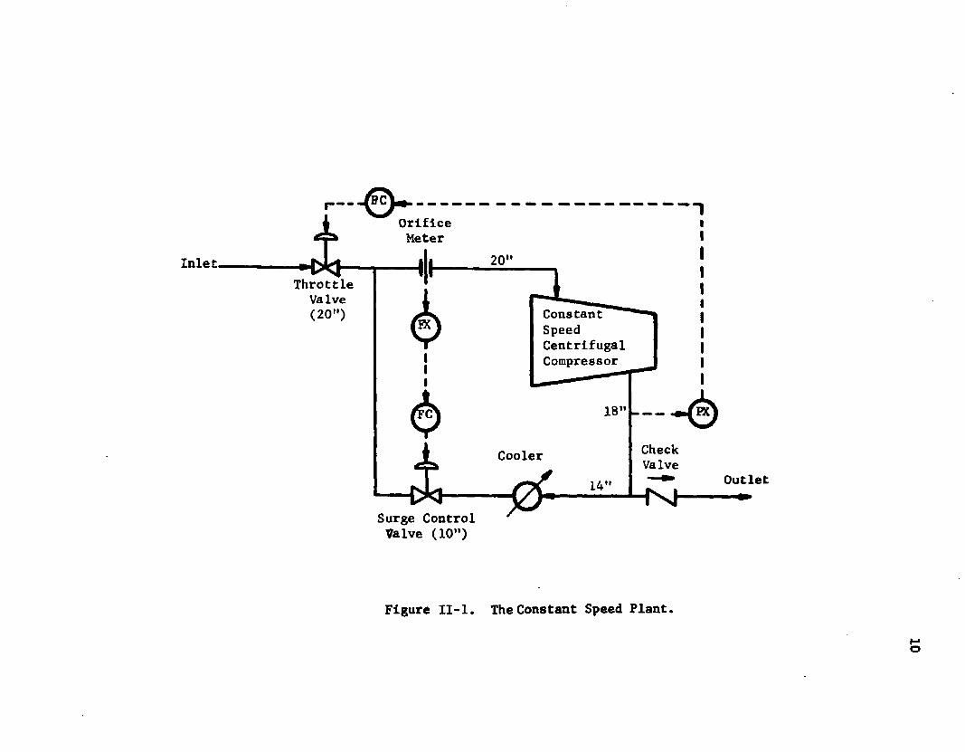
blished. It was for this reason that the relatively simple system

shown in Figure II-l was chosen for study for if the inlet and out

let systems are overly complicated the results of the simulation

may hinge upon their simulation rather than the simulation of the

compressor. However, this type of arrangement is one which can be

found in large plant air systems, fluid catalytic cracking units

and possibly in refrigeration systems [1-8].

The heart of the system is a one stage constant speed centri

fugal compressor with bypass for anti-surge control and suction

throttling for discharge pressure control. The compressor perfor

mance curve upon which the model is based was obtained from one

of the major manufacturers of centrifugal compressors. It repre

sents the constant speed performance characteristics of a compressor

which is in operation today.

OrificeMeter

InletThrottle

Valve( 20") Constant

SpeedCentrifugalCompressor

CheckValveCooler

Outlet

Surge Control Valve (10")

Figure II-l. The Constant Speed Plant.

o

11

The throttle valve Is a butterfly valve which was sized accord

ing to the procedure given by Moore [9]. The surge control valve was

sized to deliver surge flow plus twenty percent when eighty percent

open. It Is an equal percentage valve with a rangeability of 100:1.

All piping was designed so that the pressure drop would fall in the

range of 0.8 to 1.5 psl/100 feet of pipe. It was assumed that the

downstream temperature of the cooler would always equal the compressor

inlet design temperature. The complete steady state design is detail

ed in Appendix A.

Mathematical Model

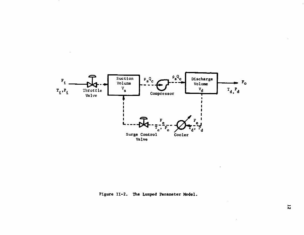
The mathematical model of the compressor is based on the Helm

holtz theory of resonators which was first applied to the centrifugal

compressor by Emmons and co-workers [10] in their successful attempt

to model surge. In order to use this theory, the suction piping

between the throttle and surge control valves was lumped into a suc

tion volume V and the discharge piping between the compressor out-

let and the first downstream restriction including the volume up to

the surge control valve was lumped into a discharge volume V,. Thisdis indicated by the dashed lines in Figure II-2. The following deri

vations were obtained based on the lumped parameter description indi

cated in Figure II-2.

Suction System

The suction system is made up of the throttle control valve

and the suction volume. Unsteady state energy and mass balances

and the standard valve equation, which is derived from the orifice

Throttle Valve

SuctionVolume

DischargeVolume

Compressor

I_____

Surge Control Valve

Cooler

Figure 11-2. The Lumped Parameter Model.

13

equation [11], are required to model It. A steady state energy bal

ance could have been used since the accumulation of energy In the

suction systems of most Industrial compressors is negligible. How

ever, this yields a nonlinear algebraic loop Implicit in the suction

temperature which requires an excess of computer time to solve.

An unsteady state mass balance about the suction volume yields

A ( P V ) « F + F - p Q . II-lat s s 1 e s cSince the suction volume V is a constant, equation II-l may be8written

ps ■ (Fi + Fe - ps V /V8- n ‘2Application of the valve equation to the throttle valve yields

the following expression for the inlet mass rate, F^, in terms of

the gas molecular weight, the inlet temperature and pressure and

the temperature and pressure within the suction volume:

F, - 1.05 C C . r'p AP .. 11-3i vi vi vi viThe pressure drop across the valve, is the difference between

the inlet pressure and the suction pressure. The density is taken

as the average of the up- and downstream densities. is the

design valve coefficient and is calculated in Appendix A. is

the function which relates the fraction of design to the vane

angle of the valve in degrees. This function, which is shown in

Figure II-3, was extracted from the work of Chinn [12] In the form

of data points and was implemented into the computer model in

the same form through an arbitrary function generator which

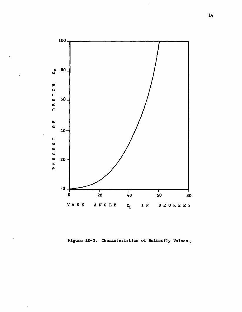
14

100

> 80 _

M60 _

40-

20 -

20 40 60

V A N E A N G L E Z* I N D E G R E E S

Figure LI-3. Characteristics of Butterfly Valves .

15

utilizes linear Interpolation. Thus the inlet mass rate Is calcu

lated according to

Neglecting any potential or kinetic energy changes, an unsteady

state energy balance taken about the suction volume may be written

where E is the molar internal energy, hifhe and hfl are respectively

the molar enthalpies of the inlet gas, the bypass loop gas and the

gas exiting the suction volume. Utilizing the four term molar heat

capacity at constant pressure relationship given by Thinh, etal [13],

the internal energy and the enthalpies may be evaluated according to

V ± - 1.05 x 9541 x Cvl /0.5(ps + PjM/CRTi) ) (P-fPs). II-4

ddt (PSV / M S) " FiVMj. + Fehe/Me - pQQcha/Mg II-5

s(Cp-r)dT - (a*-r)Ts + (b*/2)T*E - CydT -

0 0

+ (c*/3)Tg + (d*/4)Tg 11-6fTi 2 3ht - CpdT - a*Ti + (b*/2)T1 + (c*/3)Ti

+ (d*/4)Tj II-7fT,

+ (d*/4)Te II-8and

i S

+ (d*/4)Tg. II-9

16

For all cases to be considered In this study, the molecular

weight of the gas will be maintained constant at Its Initially

specified value. Consequently the M's on both sides of equation

II-5 may be canceled since they are all equal and Independent of

time. Having done this the accumulation term may be written

a W „ E ) - P , V + Vs(h„ - rTs)pB 11-10

where use has been made of the fact that for an Ideal gas, the molar

Internal energy Is the difference between the molar enthalpy and

the product of the gas constant and the absolute temperature.

Utilizing the chain rule for differentiation, the first term

on the right hand side of equation 11-10 may be expanded to give

ps V = ps V a* " r + b*Ts + c*Ts + d*Ts]*s* 11-11Substitution of this equation along with equation II-2 into equa

tion 11-10 with subsequent substitution of the results Into

equation II-5 yields after collecting terms

* _ Fi<hi - h8 + rTs) + Fe (he - hs + rT ) -psQcrTTs ------------------------------ ;---- r - s ---------- II-12a

Psvs ta*-r + b*Ts + c Ts + d TsJ where the enthalpies are given by equations II-7 through II-9.

An analysis of equation II-12aindicates that for the cases con

sidered in this study some simplifications may be in order. Utiliz

ing equations II-7 and II-9, the difference in enthalpy of the inlet

gas and the gas within the suction volume may be written as

hi - hg = (Ti - Ts) [a* + (b*/2) (Ti+Ts) + (c*/3) (T^ + T* + T T )i s

+ (d*/4)(Ti + Tg)(T^ + Tg)].

Because heat transfer through the walls of the suction piping has

17

been neglected and because Ffi, throughout this study, trill always2be maintained at approximately zero, the sum of T. and T and T. and1 8 12T may be approximated as just twice the suction temperature and twice s

the suction temperature squared respectively. This Implies that the

above equation may be written as

h -h - (T -T )[a* + b*T + c*T2 + d*T3]1 a 1 8 8 8 8where the terms in brackets are approximately equal to the bracketed

terms In the denominator of equation II-12a. Similarly, equations

11-8 and II-9 may be used to obtain

h -h - (T -T )[a* + b*T + c*T2 + d*T3]. e 8 e s s s s

The remaining terms in the numerator of equation II-12a may be

canceled because during the transient periods the sum of the inlet

and bypass flow rates is essentially equal to the flow of gas enter

ing the compressor (they are exactly equal at steady state). Uti

lizing these simplifications, the energy balance for the suction

system may be written as

T = [F.(T.-T ) + F (T -T )]/p V II-12bs i i s e e s 8 swhich, for future reference, will be termed the simplified suction

energy balance while equation II-12a is termed the ideal suction

energy balance. Equation II-12b can also be obtained from equation

11-15 if the specific heats are assumed equal and constant.

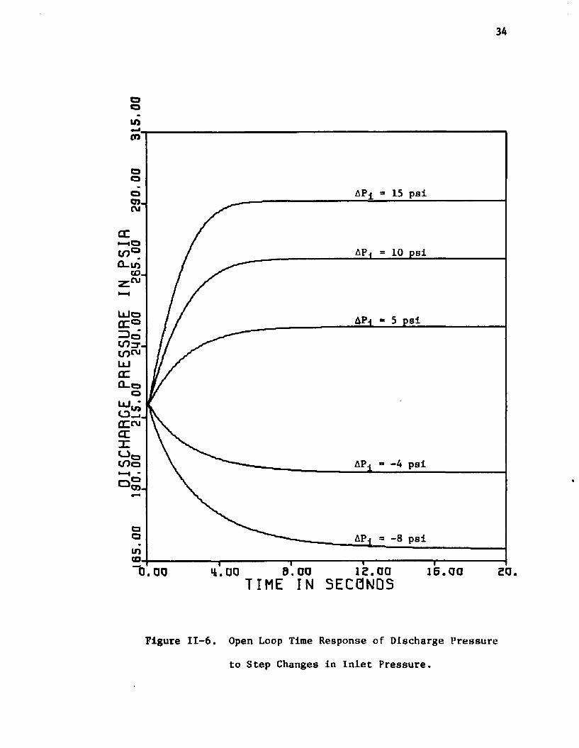
In an effort to prove that the results of these two equations

are essentially equal, the open loop results in terms of discharge

pressure versus time for step changes in the inlet temperature of

+ 30 and + 50 degrees Fahrenheit were obtained utilizing each of

them. These results are shown in Figure II-7. The simplifications

18

are so good that the two sets of four curves appear to fall exactly

on top of each other. This would not be the case If the surge con

trol valve were opened. Because of this, equation II-12a has been

Included in the summation of dynamic equations given in Table II-l

even though all of the results for the CSIGM were obtained using the

simplified suction energy balance.

Discharge System

The discharge system consists of the discharge volume V., thedsurge control valve and the cooler. To model it mathematically

requires an unsteady state mass balance, the standard valve equation

and an expression to evaluate the pressure drop across the cooler.

An unsteady state energy balance is not required for two reasons.

First, in most industrial compressor discharge systems the heat

losses are negligible. Second, in modeling the compressor an expres

sion for calculating the compressor discharge temperature is develop

ed which, based on the first reason, is taken as the temperature

within the discharge volume.

Application of the unsteady state mass balance about the dis

charge volume gives

f’ d ■ (°aQc ' Fe - V /Vd- n -13The outlet mass rate Fq represents the load demand placed on the

compressor system by the downstream unit. It was given the steady

state design value in all cases except those in which it was per

turbed.

In a manner similar to that utilized to obtain the inlet mass

rate, the valve equation can be used to obtain an expression

for the bypass mass rate, F , in terms of the downstream cooler

19

temperature and pressure, the suction temperature and pressure and

the molecular weight of the gas. However, for this valve both

critical or "choked" and subcrltical flow were accounted for in

the computer model.

In the case of choked flow for which P < 0.53 P [141 the8 — e 1 1

valve equation yields

Fe ' Cf Cve Pe " - 1 • JI-“

Cj Is a critical flow factor specified by the valve manufacturer

as 0.9 and Cve is the design Cv given in Appendix A. One of the

manufacturers of centrifugal compressors suggested utilizing the fol

lowing expression for the pressure drop across the cooler:2

AP - ij>F 11-15c e

from which P is calculated by the following expression:

Pe “ Pd " *Fe ‘ 11-16

C^e is the fraction of flew through the valve which may be calculated

according to the following expression which holds for an equal

percentage valve with rangeability of a:l

fraction flow » 1/a exp (stem position x In a) 11-17

where stem position is the ratio of the actual stem position to

the stem position when the valve is wide open. Thus the bypass

mass rate is calculated for critical flow according to

F - 0.9 x 9.74 exp (4.6 Z ) (P , - *F2) Sm 7 T ~/5.1 11-18e e a e e

20

since the rangeability was taken as 100:1.

In the case of subcrltlcal flow an expression similar to

equation II-3 is applicable. For this case the following is uti

lized:

Fft ■ 1.05 x 9.74 exp (4.6 Ze)

Compressor

The equation necessary to model the compressor results from

a steady state energy balance. Since It may not be clear why a

steady state energy balance Is used rather than an unsteady state

energy balance, a complete derivation will be given Indicating

the assumptions Implicit In the steady state balance.

An unsteady state energy balance about the compressor for

one pound of gas yields

where the Indicated Integration Is carried out over the length of

the compressor channel. If It Is assumed that the mass flow rate

Is constant throughout the compressor channel then equation 11-20

may be written

/0.5 (p8 + (Pd- ^ ) M / ( R T e)(Pd- <d£-Pg) 11-19

11-20

K dFcic "dT * H - 778 II-21

where K is designated the "channel constant" and Is evaluated

21

according toL

K « ~ 2L- . 11-22 o pcac

The left hand side of equation 11-21 represents the energy

required to accelerate the gas which Is Intuitively negligible.

Indeed, the value calculated for the "channel constant?' Is so small

for most compressors that the whole term on the left may be as

sumed zero for all time. This Is equivalent to saying that the

work performed on the gas, the enthalpy change which the gas

undergoes, is all converted to head since the difference between

the kinetic energy at the entrance and that at the exit is in

most cases negligible. Therefore the compressor is represented

by

H - 778 Ah/M 11-23

which Implies that the entire process is comprised of unsteady

state balances coupled through the above steady state balance.

As implied above, the left hand side of equation 11-23 is

the head developed by the compressor. This represents the energy

imparted to the gas by the impellers of the compressor. It is

generally accepted that H is only a function of the diameter of

the impeller, its angular velocity and the volumetric flow rate

through the compressor Qc {15-17]. For this case the diameter of

the impeller and its angular velocity are both constant and H is

a function of only Qc. The H-Qc curve used in the simulation is

shown in Figure II-4 along with the points extracted from the

design curve supplied by the manufacturer.

ocu

_J

■uu

r>1 Q 0 . 0 0 120.DO 140.00INLET FLOW 180.00160.00 flCFM

Figure II-4. The Compressor Performance Curve.INOho

23

The continuous curve shown in Figure II-4 was obtained from

a linear least squares fit of the indicated data points to an

equation of the form

which is a parabola centered at Even though the fit

does give a conservative estimate of the surge point, the point

at which the slope of the H-Qc curve is zero, it was considered

satisfactory because the first four data points were extrapolated

from the manufacturer's curve. The particular constants obtained

from the fit yielded a standard error of 1.3 percent or 350

ft-lbf/lbm which was termed good because the resolution of the

manufacturer's curve had this order of magnitude.

The term on the right side of equation 11-23 is the change

in enthalpy which one pound of gas undergoes as it is compressed.

Thus, based on this steady state analysis of the compressor, Qc

is an implicit function of Ah through the expression for the head.

Given an equation of state for the gas and a heat capacity rela

tionship, Ah, implying Qc, can be obtained through the following

sequence of calculations.

An entropy balance made about the compressor for the isentropic

compression of an ideal gas yields

Application of the equation of state for an ideal gas and the four

term ideal heat capacity relation yields the following expression

which contains only one unknown, the isentropic discharge tempera

ture Tdi:

H - ^ - A(Qc-qm)2 11-24

C (T)dinT - r Ps11-25

(r£n(p ./p ) + (a* - r)£nT a s s

+ T (b* + T (c*/2 + T d*/3))). 8 8 8 11-26

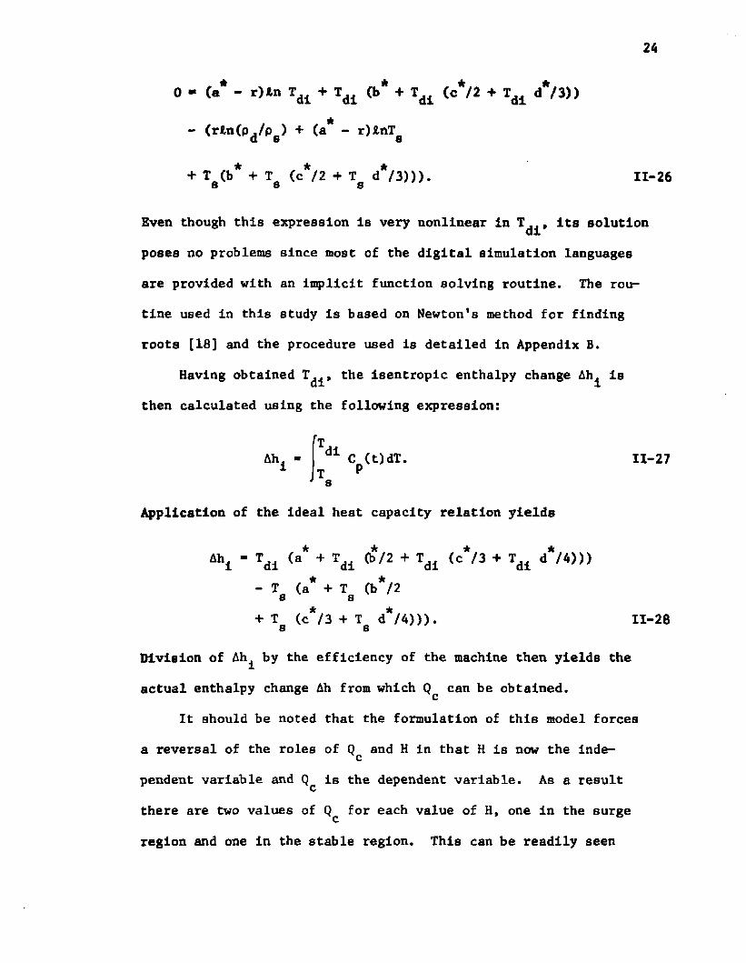
Even though this expression is very nonlinear in T ,., its solutiondiposes no problems since most of the digital simulation languages

are provided with an implicit function solving routine. The rou

tine used in this study is based on Newton's method for finding

roots [18] and the procedure used is detailed in Appendix B.

Having obtained the isentropic enthalpy change Ah^ is

then calculated using the following expression:

Division of Ah^ by the efficiency of the machine then yields the

It should be noted that the formulation of this model forces

a reversal of the roles of Q and H in that H is now the inde

region and one in the stable region. This can be readily seen

C (t)dT 11-27

Application of the ideal heat capacity relation yields

4hl - Tdl <°* + Tdl 0>*/2 + Tdl (c*/3 + Tdl d*M)))- T (a* + T (b*/2 s s+ T (c*/3 + T d*/4))). s s 11-28

actual enthalpy change Ah from which can be obtained.

cpendent variable and is the dependent variable. As a result

there are two values of for each value of H, one in the surge

25

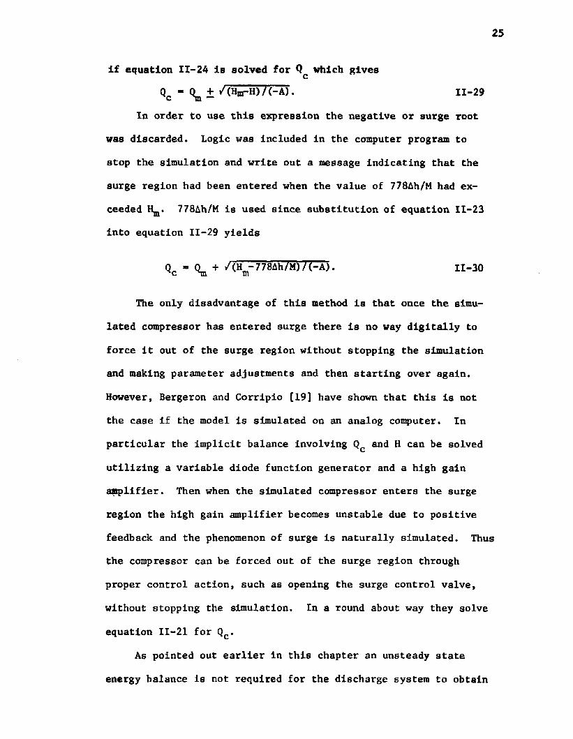
if equation 11-24 is solved for which gives

Qc - + / (HnrH) / (-A). 11-29

In order to use this expression the negative or surge root

was discarded. Logic was Included in the computer program to

stop the simulation and write out a message indicating that the

surge region had been entered when the value of 778Ah/M had ex

ceeded 778Ah/M is used since substitution of equation 11-23

into equation 11-29 yields

Qc = (^ + /(Hm-778Ah/M)/(-A). II-30

The only disadvantage of this method is that once the simu

lated compressor has entered surge there is no way digitally to

force it out of the surge region without stopping the simulation

and making parameter adjustments and then starting over again.

However, Bergeron and Corripio [19] have shown that this is not

the case if the model is simulated on an analog computer. In

particular the implicit balance involving Qc and H can be solved

utilizing a variable diode function generator and a high gain

amplifier. Then when the simulated compressor enters the surge

region the high gain amplifier becomes unstable due to positive

feedback and the phenomenon of surge is naturally simulated. Thus

the compressor can be forced out of the surge region through

proper control action, such as opening the surge control valve,

without stopping the simulation. In a round about way they solve

equation 11-21 for Q£.

As pointed out earlier in this chapter an unsteady state

energy balance is not required for the discharge system to obtain

26

the discharge temperature because Td is calculated from an

expression used In modeling the compressor. The necessary

expression which contains only one unknown, , is obtained from

the thermodynamic equation to calculate Ah which is

Substitution of the expression for the heat capacity yields, after

integration, the following expression which can be solved for Td

with another implicit function solving routine:

The method used to solve this expression is also Newton's and the

procedure is also detailed in Appendix B.

To facilitate a more complete analysis of the model, an infor

mation flow diagram for the entire system which has been developed

to this point is shown in Figure II-5. The accompanying dynamic

equations are given in Table II-l.

11-31

0 - Td(a* + Td (b*/2 + Td (c*/3 + Td d*/4)))

- (Ts(a* + Ts (b*/2 + Tfl (c*/3 + Ts d*/4)))

+ Ah). 11-32

T_ P3 fEqn. 10 Eqn. 6 »— -4-» Eqn. 1

IEqn. 9 vi

rsEqn. 2

Ah Eqn. 25

Eqn. 11

Eqn. 14 or 15

Eqn. 18 ve

./ S_AhT T Eqn. 23

~ € ZAh

TI.

Eqn. 22

U

Ahj

Eqn. 19 Eqn. 13

Eqn. 21

Idi Eqn. 20

Z T ~

sT T

Figure II-5. Information Flow Diagram for Open Loop CSIGM.

28

TABLE II-l

CSIGM DYNAMIC EQUATIONS

Suction System

Mass balance pB - (Fi + Fe - P8QC)/V8 ^

Energy balance Ta -P8Vo[a*-r+Ta(b*+T(c*+T d*))] (2)

Inlet enthalpy hi - Ti(a"+T1(b’*/2+Ti(c,'/3+Tid*/4))) (3)

Bypass loopenthalpy he - Te(a*+Te(b*/2+Te(c*/3+Ted*/4))) (4)

Suction enthalpy h = Tc(a*+T)a(b*/2+T (c*/3+Tfid*/4))) (5)8 8 o 3 8

Inlet massrate ? ± « 1.05 Cvl^pviAPvl (6)

Throttle valvedensity pvl - 0.5 (p8 + P^/CRT^) (7)

Throttle valvepressure drop 4Pyi «* P^ - Pg (8)

Throttle _valve Cy C ^ - C^fCZj) (*See below) (9)

Equationof state P « pflRT /M (10)

S s 3

*f(Z^) is the function which relates the fraction of design C to the throttle valve vane position. It is shown in Figure II-3.

29

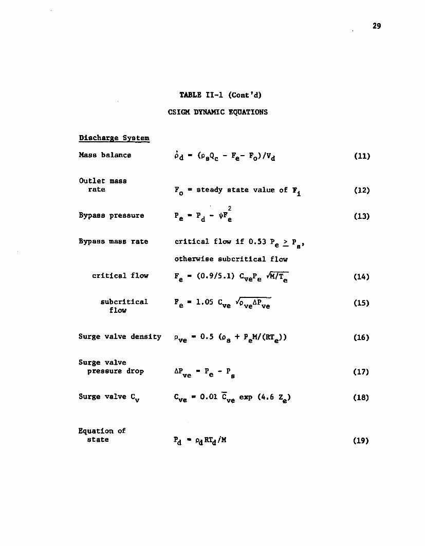
Discharge SystemMass balance

Outlet mass rate

Bypass pressure

Bypass mass rate

critical flow

subcriticalflow

Surge valve density

Surge valve pressure drop

Surge valve Cv

Equation of state

TABLE II-l (Cont'd)


Pd " (PSQC " Fe" Fo>/Vd (ID

Fq » steady state value of F^ (12)

Pe - Pd - ¥ * * (1 3 )

critical flow if 0.53 Pe >_ Pfi,

otherwise subcritical flow

Fe - (0.9/5.1) CvePe ^S7t^ (14)

Fe ■ 1-05 cve y»veiPve »*>

Pw - 0.5 (p. + PM/(RT )) (16)

AP - P - P (17)ve e s v 1

cve *0.01 C exp (4.6 Z.) (18)

Pd " PdRTd^M (I9)

30

Compressor

Isentropic discharge temperature

Isentropic enthalpy change

Actual enthalpy change

Discharge temperature

TABLE II-l (Cont'd)CSIGM DYNAMIC EQUATIONS

AS - 0 - (a* - r) An Tdl

+ Tdi (b* + Tdi(c*/2 + Td±d*/3))

- [rin(pd/p8) + rAnTs

+ T (b* + T (c*/2 + T d*/3))] (20)O 9 S

Ah± - Tdl (a* + Tdl(b*/2 +

Tdi(c*/3 + Tdid*/4))>

- [T (a* + T (b*/2 +O O

Ts(c*/3 + Ts d*/4)))] (21)

Ah = Ah^n (22)

0 - Td (a* + Td (b*/2 + Td(c*/3 +

Tdd*/4))) - [Ts (a* + Tg(b*/2 +

Ta(c*/3 + Tsd*/4))) + Ah] (23)

X

31

Energy balance

Volumetric flow

TABLE II-l (Cont'd)


(24)

(25)

CWxi 778Ah/M<Hmln

Hgiin and Qq a x are respectively the

head and flow rate at the "stonewall."

H - 778 Ah/M

rate

surge; 778Ah/M >

Q + /(H -778Ah/M)/(-A) m m

32

Integration Method

In order to carry out the simulation of the CSIGM on the

digital computer, an integration method had to be determined.

Several choices were available since SL1 is provided with Euler,

trapezoidal, a four-point predictor, Adams-Moulton, fourth order

Runge-Kutta-Gill and Runge-Kutta with error control [20] while

CSMP is provided with rectangular, trapezoidal, Simpson's,

Adams-second order, fourth order Runge-Kutta and a Milne fifth-

order predictor-corrector [21].

Initially the fourth order Runge-Kutta method with a fixed

integration step size of 0.01 seconds was chosen. This step size

was the upper end of a range of step sizes which produced comparable

open—loop simulation results. However, when the closed-loop simu

lation, initially at steady state, was executed with no disturbances,

all of the variables slowly drifted away from their steady state

values.

Because of this slow drift the lower order Integration tech

niques, Euler, rectangular and trapezoidal, were examined. It was

found that when using the optimum integration step size, each of

these techniques yielded comparable open-loop as well as closed-

loop simulation results and required much less computer time. Too,

when the closed-loop simulation, initially at steady state, was

executed with no disturbances, all of the variables remained

at their steady state values. The trapezoidal method with an

integration step size of 0.02 seconds was chosen over the other

two lower order methods because it is the only integration technique,

other than the Runge-Kutta, which CSMP and SL1 have in common.

33

A common integration technique was desired because Initial

debugging and testing was carried out on the XDS-E5 which is operat

ed open shop. Subsequent runs were then carried out on the IBM-

360/65 because facilities were available to produce the plots mechan

ically. These facilities consisted of a Calcomp plotter and the

necessary tape units.

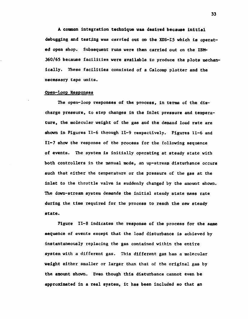
Qpen-Loop ResponsesThe open-loop responses of the process, in terms of the dis

charge pressure, to step changes in the inlet pressure and tempera

ture, the molecular weight of the gas and the demand load rate are

shown in Figures II-6 through II-9 respectively. Figures II-6 and

II-7 show the response of the process for the following sequence

of events. The system is initially operating at steady state with

both controllers in the manual mode, an up-stream disturbance occurs

such that either the temperature or the pressure of the gas at the

inlet to the throttle valve is suddenly changed by the amount shown.

The down-stream system demands the initial steady state mass rate

during the time required for the process to reach the new steady

state.

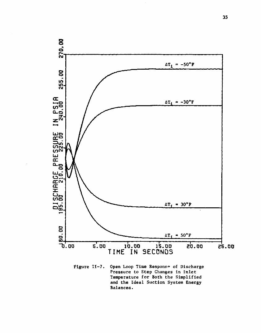
Figure II-8 indicates the response of the process for the same

sequence of events except that the load disturbance is achieved by

Instantaneously replacing the gas contained within the entire

system with a different gas. This different gas has a molecular

weight either smaller or larger than that of the original gas by

the amount shown. Even though this disturbance cannot even be

approximated in a real system, it has been Included so that an

DISC

HARG

E PR

ESSU

RE

IN PS

IA65

.00

190.

00

215.

00

2M0.

0G

265.

00

290.

00

315.

00

34

AP^ = 15 psi

APj = 10 psl

AP4 = 5 psi

-4 pslAP

AP-t = -8 psi

8 . 00 1 5 . oaTIME IN SECONDS

Figure II-6. Open Loop Time Response of Discharge Pressure

to Step Changes in Inlet Pressure.

01SCH

fiRCE

PRES

SURE

IN

PSIR

80.0

0 19

5.00

21

0.00

22

5.00

2*

40,0

0 25

5.00

27

0,00

i i

i

j

i i

i

35

AT

-30°FAT.

AT.

50°FAT

.00 S. DO 10 .00 15.00 20.00 25.00TIME IN S EC ONDSFigure II-7. Open Loop Time Response of Discharge

Pressure to Step Changes in Inlet Temperature for Both the Simplified and the Ideal Suction System Energy Balances.

DISC

HARG

E PR

ESSU

RE

IN PS

IA-1

80.0

0 10

5.00

21

0.00

22

5.00

2U

0.00

25

5.00

27

0.0

.4-

«----

----

1—■ r

1 1

1

36

AM = 3 lb/mole

AM ■= 2 lb/mole

AM = 1 lb/mole

AM ■ -1 lb/mole

AM = -2 lb/mole

AM = -3 lb/mole

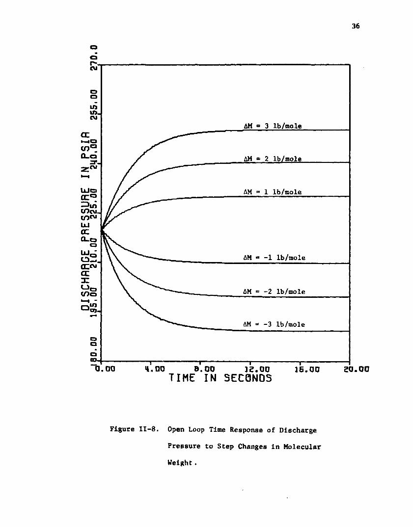
>1.00 B. OO 12.00 16.00 20.00TIME IN S EC ONDS

Figure II-8. Open Loop Time Response of Discharge

Pressure to Step Changes in Molecular

Weight .

37

in

-0.15 FdeSignAF.design

CM

-0.05 FdesignAFCL

L U o£ E °3 qcn—UJa:

0.05 Fdesign

.designAF,

design

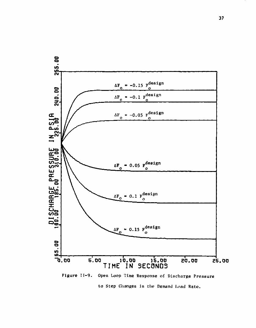
(O.5.00 15.0010.0000 20.00 25.00TIME IN S EC ONDS

Figure I1-9. Open Loop Time Response of Discharge Pressure

to Step Changes in the Demand Load Rate.

38

evaluation may be made for a gas differing In composition from the one upon whlchthe steady state design Is based.

It should be pointed out that the more realistic disturbance of

making step changes in molecular weight in the feed gas can only be

achieved by changing n-1 compositions at the inlet to the throttle

valve, where n is the number of components in the gas. To simulate

this would require a total mole balance along with n-1 component bal

ances for both the suction and discharge systems. This means there

would be 2+ 2(n-1) or 2n additional nonlinear-coupled-first-order-

ordinary differential equations in addition to the more coupled and

more nonlinear energy balance for the suction system. Since the

unrealistic disturbance does provide a qualitative indication of the

system response, but with much less complication, the additional 2n

differential equations have not been included in the model.

The curves shown in Figure II-9 are the response of the system

to the Indicated step changes in the demand load rate. They repre

sent the response of the uncontrolled compressor to changes in the

mass flow rate demanded by the unit downstream of the compressor

system.

In order to obtain the responses shown in Figure II-6, the

inlet pressure, which appears only in the throttle valve equation,

was changed at time zero for each of the five simulation runs by the

amounts shown. The remaining variables were set to their steady state

values at time zero and then allowed to come to their new steady state

values. Table II-2 gives the new steady state values of the discharge

pressure, the head and the volumetric flow rate through the compressor.

It also gives the time required for the system to reach 99.5 percent

39

TABLE II-2

OPEN-LOOP RESULTS FOR INLET PRESSURE CHANGES(CSIGM)

Api pd88 tc Hss _ ss Qc(psi) (psia) (sec) (ft-lbf/lbm) (acfs)

15 293.75 5.5 21662. 246.8610 272.44 7.2 21342. 261.615 247.97 9.0 20736. 278.3

-4 194.91 12.9 18506. 314.74-8 167.46 14.5 16783. 334.43

TABLE II-3OPEN-LOOP RESULTS FOR INLET TEMPERATURE CHANGES

(CSIGM)

AT±(°F) Pd8S(psia) (sec)

Hss(ft-lbf/lbm)

Q 88(acfs)

50 181.31 14.1 17542. 326.2630 196.22 13.8 18513. 314.64

-30 245.38 11.6 20649. 280.22-50 263.12 10.7 21111. 268.85

TABLE I1-4

OPEN-LOOP RESULTS FOR MOLECULAR WEIGHT CHANGES(CSIGM)

AM(lb/mole) PdSS(psia) Cc(sec)

HSS(ft-lbf/lbm)

Q 88 (acfs)

321

-1-2-3

251.43241.00230.50209.45199.39189.17

10.410.7 11.011.511.7 11.9

20749.20460.20120192611772315321

278.00284.17290.63304.46311.92319.43

40

of the change in discharge pressure. This time is proportional to

the time constant and is thus characteristic of the process. Note that

as AP^ varies from 15 to -8 psi the characteristic time varies from

5.5 to 14.5 seconds Indicating that the system time constant is strong

ly dependent upon the inlet pressure. Note also that Increases for

the same changes in AP., This explains the Increase in t since1 cT a V/Qc (a means proportional) implying that Ax a "AQc and since

t a x then At a - AQ where At and AQ are the indicated t and c c c c c cQ minus the t and Q at AP, ■ 0. c c c 1

In a similar manner, the responses shown in Figure II-7 were ob

tained. However, in this case, the inlet temperature, which appears

in both the energy balance and the throttle valve equations, was

changed. Note that for this case the initial change in discharge

pressure is in the opposite direction from the final change in dis

charge pressure. An explanation of this phenomenon results from an

examination of the discharge pressure equation in which opposing

changes in the discharge temperature and density alternately predomi

nate. For an increase in the inlet temperature, the valve equation

dictates that the inlet mass rate and hence the mass throughput of the

compressor will decrease. Since the load demand on the outlet of the

discharge system is maintained at a fixed rate, the discharge density

tends to decrease to a lower final value. However, because of the

assumption of no heat losses and because the bypass rate is essentially

zero, the suction temperature immediately approaches the increased in

let temperature. This sudden rise in the suction temperature manifests

itself as a corresponding rise in the discharge temperature which

causes the discharge pressure to rise above its initial value. This

41

rise continues until the decreasing discharge density predominates

at which time the discharge pressure begins falling as is predicted

by the steady state thermodynamic head equation.

Table II-3 gives the new steady state values which were achieved

by the discharge pressure, the head and the volumetric flow rate

through the compressor along with the time required to reach 99.5

percent of the change in the discharge pressure. Unlike the above

case, t decreased as the disturbance was changed from its maximum

positive to its maximum negative value. The same explanation as

given above in terms of the change in Q holds here also.cThe responses shown in Figure II-8 were achieved by initially

changing the gas from pure propane to a mixture of propane and

n-butane for the positive AM’s and from pure propane to a mixture of

propane and ethane for the negative AM's. These changes were accom

plished by specifying an initial mole fraction of either n-butane with

the mole fraction of ethane set to zero or specifying an initial mole

fraction of ethane with the n-butane mole fraction set to zero. The

following equations, which are in the initial section of the computer

program, were utilized to calculate the mole fraction of propane, the

molecular weight of the gas and the constants of the heat capacity

relation:

Y = P 1 - y e - y b 11-33

M = Vp + y e m e + Yr t 11-34*a ■m

* *a PYP + * ey e + “*by b 11-35

*b ■m* *b Y + b_Y + p p E E

*bBYB 11-36

*c ■m* *V p + ceYe +

*cby b 11-37

42

and

4 - V p + V e + V b •The values obtained for each of the above parameters were then

substituted into each of the dynamic equations containing them. The

dynamic simulation was then initiated and executed until the new

steady state was achieved. Table II-4 shows the steady state results

as In the other two series of disturbances. As in the first case,

the characteristic time increases as the disturbance is varied from

maximum positive to maximum negative. The same analysis in terms

of Q and t explains the trend Indicated for t . c cThe responses shown in Figure II-9 were obtained by changing

the demand load rate from the design load rate by + 15, + 10 or + 5

percent of the design load rate as is shown. All other variables

were set equal to their respective design values, the simulation was

started and each variable was allowed to achieve its new steady state

value. The new steady state values of the discharge pressure, the

head and the volumetric flow rate along with the time required to

reach 99.5 percent of the change in are shown in Table II-5.

Note that the trend indicated for t^, which can be explained by the

x - Qc analysis given earlier, is almost the exact inverse of the

tc trend for There does not appear to be any clear-cut explana

tion for this because of the complicated interrelationships among

the variables of the model.

Closing the Loop

To date the state of the art of the development and design of

chemical processes does not entail the use of dynamic models though

A3

TABLE II-5

OPEN-LOOP RESULTS FOR LOAD DEMAND CHANGES(CSIGM)

ZAFo088d(psia)

£88(Secs)

Hss(ft-lbf/lbm)

qssc(acfs)

15 173.26 15.5 15A91. 3A7.0310 190.58 1A.6 17185. 330.195 206.3 12.5 18591. 313.64

-5 231.32 8.5 20597. 281.34-10 2A0.08 7.0 2122A. 265.5-3,5 .. . 2A6.06 5.0 21614. 249.84

It appears that the dynamic design Is just over the horizon. The

dynamic model does, however, offer unlimited possibilities In the

development of control schemes for the statically designed chemical

process. Most Importantly, they enable the control engineer to tune

control loops In some definable optimal sense and enable him to uti

lize disturbances which would not be permitted In the actual plant

because of safety considerations, product quality considerations and

the like.

The remainder of this chapter is devoted to demonstrating that

the dynamic model of the centrifugal compressor can be utilized to

obtain tuning constants which yield more superior responses than do

tuning constants obtained from a classical tuning procedure. The

discharge pressure control loop shown in Figure II-l will be closed

with a classical pneumatic controller. The loop is depicted in

Figure 11-10 using block diagram notation.

Dynamics of the Control Valve and Transmission Line

An analysis of the open-loop responses given earlier indicates

that the process has a time constant in the neighborhood of a few

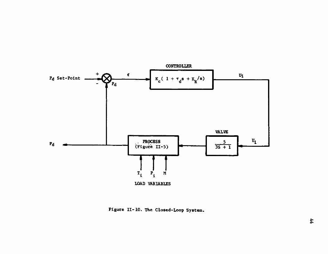
CONTROLLER

Pd Set-Point

VALVE

3S + 1. PROCESS (Figure II-5)

T P i i M

LOAD VARIABLES

Figure 11-10. The Closed-Loop System.

45

seconds. Since this Is a relatively small time constant, the

dynamics of the control valve and transmission line cannot be neglected as is the case for most chemical processes. Harriot has

suggested that the valve and transmission line dynamics can be ade

quately represented by a simple first order lag with a time constant

of three seconds [22]. This is indicated in Figure 11-10 by the

transfer function given in the block labeled valve.

A conversion from the Laplace domain to the time domain is

required to more easily implement these dynamics into the computer

program. This is readily accomplished and is given below.

Assume the steady state relation between the controller output

pressure and the vane position of the throttle valve is linear.

Further assume that the up- and downstream processes dictate that

the throttle valve must close while the surge valve must open upon

the loss of instrument air so as to provide maximum protection for

the compressor. Then the expression which relates the controller

output in psig to the throttle valve vane position in degrees can

be written

Z ± - 60 - 5 (U - 15). 11-39

Note that the wide open position of the throttle valve is 60° which

is the value suggested by Chinn because of force considerations.

Note also that the slope of this expression is 5°/psig which is the

gain given in the valve transfer function shown in Figure 11-10,

The steady state design given in Appendix A indicates a steady

state inlet mass rate of 170.5 lbm/sec. With the aid of equation

II-4, the steady state value of is found to be 0.65. Utilizing

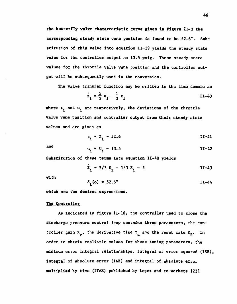
46

the butterfly valve characteristic curve given in Figure 11-3 the

corresponding steady state vane position is found to be 52.6°. Sub

stitution of this value into equation 11-39 yields the steady state

value for the controller output as 13.5 pslg. These steady state

values for the throttle valve vane position and the controller out

put will be subsequently used in the conversion.

The valve transfer function may be written in the time domain as

"i ' 3 "l ‘ 3 *1 II'40

where z^ and u are respectively, the deviations of the throttle

valve vane position and controller output from their steady state

values and are given as

s4 - Z - 52.6 11-41

“ d ui “ Ui " 13,5 11-42Substitution of these terms into equation 11-40 yields

with

Z ± - 5/3 U± - 1/3 Z ± - 5 11-43

Z±(o) - 52.6° 11-44

which are the desired expressions.

The Controller

As indicated in Figure 11-10, the controller used to close the

discharge pressure control loop contains three parameters, the con

troller gain K , the derivative time x. and the reset rate K_. In c d Rorder to obtain realistic values for these tuning parameters, the

minimum error integral relationships, integral of error squared (ISE),

Integral of absolute error (IAE) and integral of absolute error

multiplied by time (ITAE) published by Lopez and co-workers [23]

47

were utilized. Their formulae give the controller tuning parameters

in terms of the process gain K, the process time constant t and the

process dead-time (transportation lag or time delay) 0, obtaineddfrom an open-loop process reaction curve. The latter is a plot of

the discharge pressure (controlled variable) versus time for a step

change in the controller output, AU^, with the controller in the

manual mode. (Reference 23 has an excellent discussion of the pro

cess reaction curve.)

Since no actual process reaction curves were available, the

model was used to generate them. This is as near to actual condi

tions as is possible. The nonlinearities of the process, Including

the control valve characteristics, caused the parameters obtained

from the process reaction curve to be a function of the size and

direction of the step change in the controller output. To circum

vent this, eight process reaction curves covering the range

-1.4 AUj. ^.1.4 were utilized. They are included in Appendix C

along with the necessary geometric construction to obtain the param

eter values which are given in Table II-6. These three sets of

eight parameter values were plotted against AU^ and the curves

obtained were extrapolated to zero step size. These plots are shown

in Figures 11-11, 11-12 and 11-13 and the parameters obtained at

AU. ■ 0 are: K = 11.2 psi/°, x = 4.84 seconds and 0 , = 0.87 seconds,l aSubstitution of these values into Lopez’s formulae yielded the fol

lowing best controller parameters which are based on IAE:

48

TABLE II-6

PROCESS REACTION CURVE RESULTS (CSIGM)

ui(psig)AU±

(Ui-Ui88)APd

(Pd-Pd88)K

(APd/AU±)T

(sea) / 9,3 (sec.]

14.9 1.4 11.72 8.37 4.4 0.71

14.5 1.0 8.77 8.77 4.4 0.78

14.0 0.5 4.81 9.62 4.6 0.79

13.75 0.25 2.55 10.2 4.66 0.84

13.25 -0.25 -3.2 12.8 5.08 0.92

13.0 -0.5 -7.23 14.46 5.42 0.96

12.5 -1.0 -17.77 17.77 5.9 1.05

12.1 -1.4 -29.75 21.25 6.48 1.1

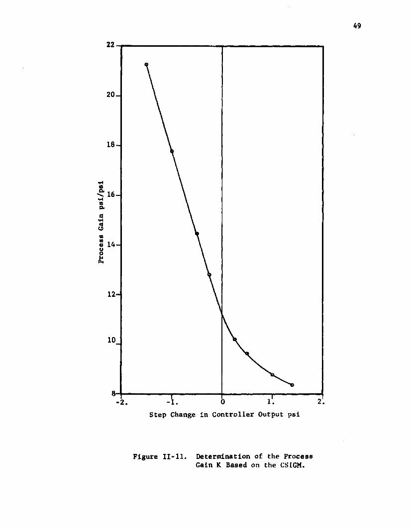
20-

18-

< 16-

12-

Step Change in Controller Output psl

Figure 11-11. Determination of the Process Gain K Based on the CSIGM.

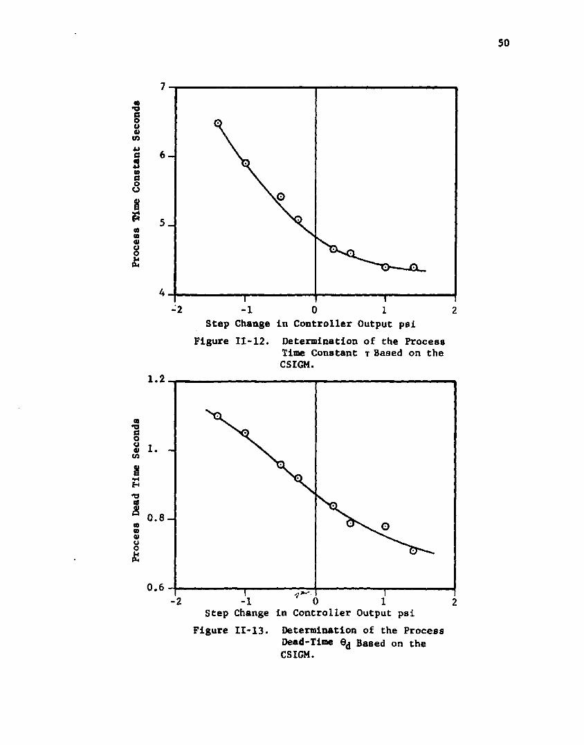
Process

Dead

Time

Seconds

Process

Time

Constant

Seco

nds

6 -

5 _

2 -1 0 1 2Step Change in Controller Output psi

Figure 11-12. Determination of the Process Time Constant t Based on the CSIGM.

0.8 -

0.6Step Change in Controller Output psi

Figure 11-13. Determination of the Process Dead-Time 0d Based on the CSIGM.

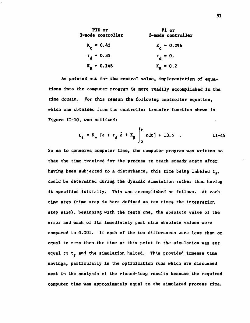
51

PID or 3-node controller

PI or 2-node controller

K - 0.43 K - 0.296 ccTd - 0.35

Kr - 0.148 K r - 0 . 2

As pointed out for the control valve, Implementation of equa

tions Into the computer program Is more readily accomplished In the

time domain. For this reason the following controller equation,

which was obtained from the controller transfer function shown In

Figure 11-10, was utilized:

So as to conserve computer time, the computer program was written so

that the time required for the process to reach steady state after

having been subjected to a disturbance, this time being labeled t^,

could be determined during the dynamic simulation rather than having

It specified initially. This was accomplished as follows. At each

time step (time step is here defined as ten times the integration

step size), beginning with the tenth one, the absolute value of the

error and each of its immediately past nine absolute values were

compared to 0.001. If each of the ten differences were less than or

equal to zero then the time at this point in the simulation was set

equal to t^ and the simulation halted. This provided immense time

savings, particularly in the optimization runs which are discussed

next in the analysis of the closed-loop results because the required

computer time was approximately equal to the simulated process time.

tui - Kc [e + Td e + Kr edt] + 13.5 11-45o

52

Closed Loop Responses

Utilizing these two sets of classically determined tuning

constants, the responses in Figures 11-14 through 11-21 were deter

mined. Figures 11-14 and 11-15 indicate the closed loop compressor

responses for + 5% changes in the demand load rate while Figures 11-16

and 11-17 indicate the responses for + 5 psi changes in the discharge

pressure set point. Responses to disturbance inputs in inlet pres

sure of 5 psi, in inlet temperature of + 10°F and in molecular

weight of 3 lbm/mole are shown in Figures 11-18 through 11-21.

To demonstrate that the dynamic model can be utilized to obtain

tuning constants which yield more optimal responses than do the con

ventionally determined tuning constants, an optimization technique

utilizing a pattern search [24] was implemented into the terminal

section of the simulation program. Values for the 3-mode controller

tuning parameters were obtained which minimized the integral of the

absolute error (IAE), for each of the disturbances and an additional

set was obtained which minimized the integral of the error squared

(ISE) for the demand load disturbances. The results of the optimi

zation runs are given in Table II-7, with some pertinent comments.

The simulation results utilizing the optimal parameters are also

shown in Figures 11-14 through 11-21 for easy comparison. These

results are labeled the optimal controller.

Two sets of optimal parameters were obtained for the load demand

rate disturbances to further demonstrate the ease and flexibility of

tuning with a dynamic model. This could have just as easily been

accomplished for each of the other disturbances but the responses in

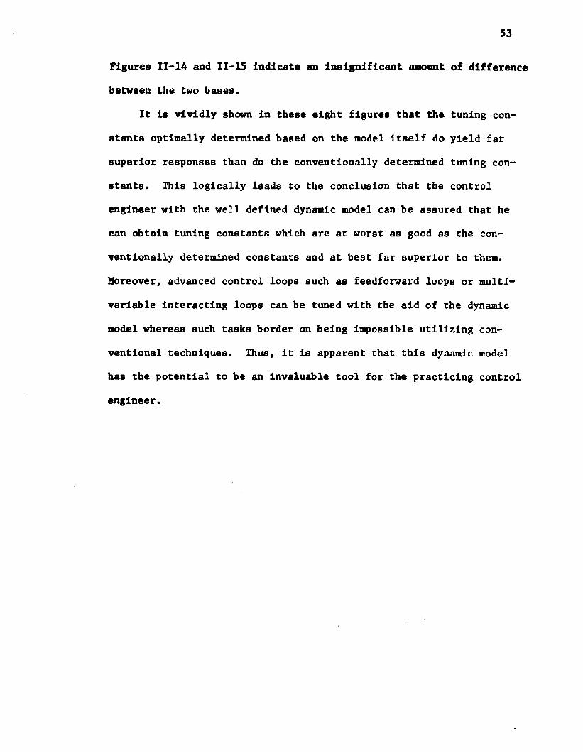
53

Figures 11-14 and 11-15 Indicate an Insignificant amount of difference

between the two bases.

It Is vividly shown In these eight figures that the tuning con

stants optimally determined based on the model itself do yield far

superior responses than do the conventionally determined tuning con

stants. This logically leads to the conclusion that the control

engineer with the well defined dynamic model can be assured that he

can obtain tuning constants which are at worst as good as the con

ventionally determined constants and at best far superior to them.

Moreover, advanced control loops such as feedforward loops or multi-

variable interacting loops can be tuned with the aid of the dynamic

model whereas such tasks border on being impossible utilizing con

ventional techniques. Thus, it Is apparent that this dynamic model

has the potential to be an invaluable tool for the practicing control

engineer.

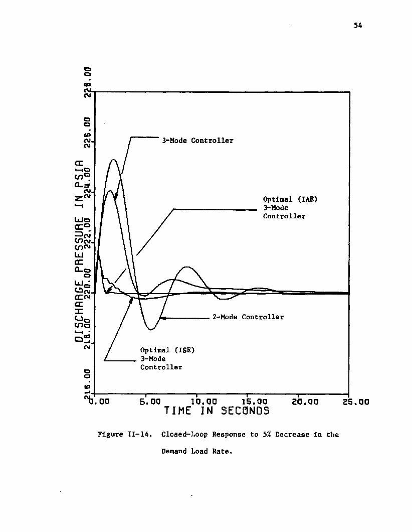
o o

CM.CM

3-Mode Controller

Optimal (IAE)3-ModeController

2-Mode Controller

CDCM Optimal (I8E)

3—Mode Controller

to5.00 15.0000 1 0 . 0 0 25TIME IN SECONDS

Figure 11-14. Closed-Loop Response to 5% Decrease in the

Demand Load Rate.

55

oicuCM3-Mode Controller

Optimal (ISE and IAE)3—ModeController

2-Mode Controller

15.00S. 00 SS.00.00t i m e i n s e c o n d s

Figure 11-15. Closed-Loop Response to 5% Increase in the

Demand Load Rate F .

DISC

HARG

E PR

ESSU

RE

IN PS

IA<220.00

221.

00

222.

00

223.

00

224.

00

225.

00

226.

00cj_ i

i i

i i

i

56

Optimal 3-Mode Controller

2-Mode Controller

3-Mode Controller

.00 5.00 10.00 15.00TIME IN SECONDS SO. 00 25.00

Figure 11-16* Closed-loop Response to 5 psl Step

Change in Set-Point for the CSIGM.

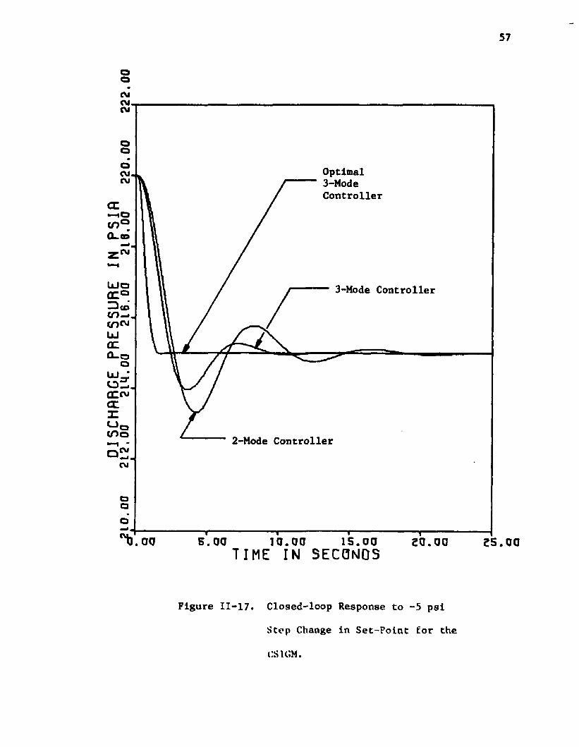
DISC

HARG

E PR

ESSU

RE

IN PS

IA10

.00

212,

00

21M

.00

216.

00

216.

00

220.

00

222.

00

57

Optimal 3-Hode Controller

3-Mode Controller

2-Mode Controller

15.0000 1 0 . 0 0TIME IN SECONDS

Figure 11-17. Closed-loop Response to -5 psl

Step Change in Set-Point for the

CS1GM.

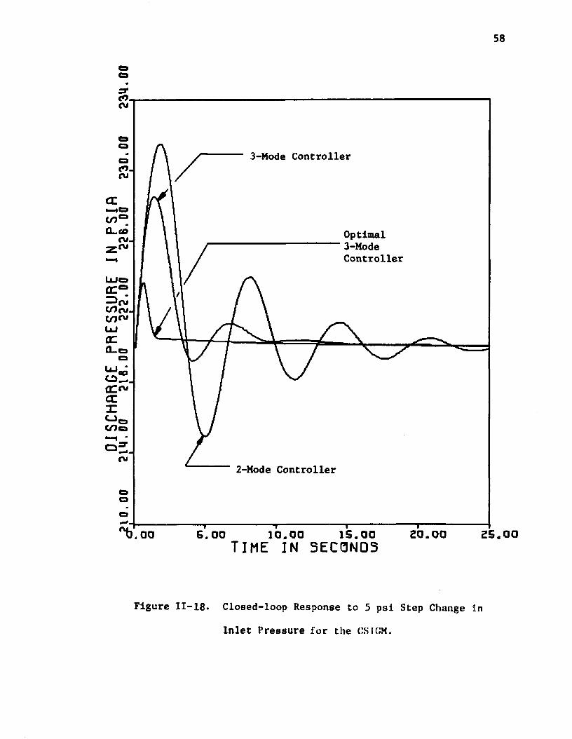
DISC

HARG

E PR

ESSU

RE

IN PS

IA10

.00

214.

00

210.

00

222.

00

226.

00

230.

00

234.

00

58

3-Mode Controller

Optimal3-ModeController

2-Mode Controller

Z S . 0 015.005.00.00 TIME IN S ECONOS

Figure 11-18* Closed-loop Response to 5 psl Step Change In

Inlet Pressure for the CSKIM.

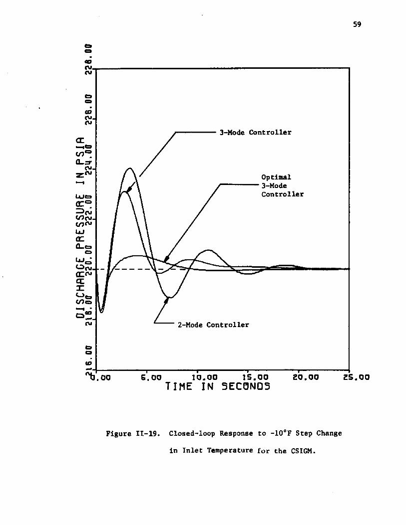
01SCH

flRCE

PRES

SURE

IN

PSIfi

16.

Off 2

18

.Off

220.

00

222.

00

22M

.00

226.

00

226.

00

59

3-Mode Controller


2-Mode Controller

15.00 Z S .0 0ZO. OOG, OO 10.0000 TIME IN S EC ONDS

Figure 11-19. Closed-loop Response to -10°F Step Change

In Inlet Temperature for the CSIGM.

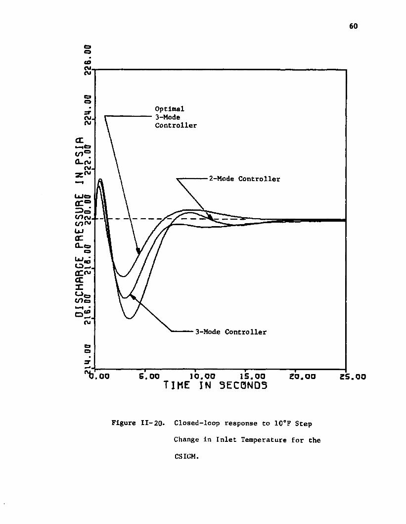
60

coCM.CM


CM,CM

2-Mode Controller

«*»CM

3-Mode Controller

6.00 15.0000 20.00 25.0010.00t i m e i n s e c o n d s

Figure II-20* Closed-loop response to 10°F Step

Change in Inlet Temperature for the

CSIGM.

cn,CNJ

CDCM,CM

3-Mode Controllercn


( D O•— i -o 2 ,

CM 2-Mode Controller

CDQ10.00 15.00TIME IN S EC 0N03

Figure 11-21. Closed-loop Response to 3 lbm/mole

Step Change in Molecular Weight

for tlie CSIGM.

TABLE II-7 OPTIMIZATION RESULTS

(CSIGM)

Disturbance Kc Td Comments

AF - 0.05 Fdeslgn o o 20.64.62

0.0020.01

0.250.44

based on ISE based on IAE

AF - -0.05 Fd68lgn o o 1.93.66

0.630.3

1.80.5

based on ISE based on IAE

AP®P - 5 psl 2.03 0.025 0.54 steady state reached after only 5.6 seconds

APjP - -5 psl o 3.68 0.025 0.64 steady state reached after only 3 seconds

ATt - -10°F 1.61 0.40 1.6 steady state reached after 16 seconds

AT_ « 10°F 0.525 0.325 1.25 steady state reached after 17 seconds

AP^ - 5 psl 2.00 0.10 0.50e £ 0.4 after 3 seconds e 0.1 after 16 seconds steady state after 31 seconds

AM ■ 3 lbm/mole 3.35 0.175 0.625 steady state reached after only 3 seconds

3-mode controller settings: K *» 0.43, * 0.148, t , ■ 0.3512-mode controller settings: - 0.296, « 0.2

63

A lumped parameter dynamic model of the constant speed centri

fugal compressor suitable for Implementation on either an analog,

digital or hybrid computer has been developed In terms of the

compression of an ideal gas or mixture of ideal gases. It was deve

loped so that no other data other than that provided to the plant

personnel by the compressor manufacturer In the form of the charac

teristic performance curves is required. The performance curve uti

lized represents the performance of a compressor which is in operation

today. It was obtained from one of the major compressor manufac

turers.

The model has been successfully tested with both open and

closed loop results having been obtained through the utilization of

the digital simulation languages CSMP and SL1. The assumption of

constant heat capacity in the suction system of the compressor has

been suggested and proven to be a valid simplification. The use of

an unsteady state suction energy balance for determining the suc

tion temperature rather than the steady state suction energy balance

was utilized because the steady state balance yields a very non

linear algebraic loop implicit in the suction temperature which

requires excess computer time to solve.

The open loop discharge pressure response curves for distur

bances in inlet pressure, inlet temperature and load demand rate

indicate that the centrifugal compressor is very nonlinear. The

initial change in discharge pressure resulting from disturbances in

the inlet temperature are in the opposite direction from the final

change. This results because the discharge density and temperature

64

changes are in opposite directions with the rate of change of discharge

temperature being the larger during a very short time interval im

mediately following the disturbance. The nonllnearltles associated

with inlet pressure disturbances were found to be similar to those

associated with demand load rate disturbances with those resulting

from increases in the demand load rate being similar to those result

ing from decreases in inlet pressure and vice versa.

The discharge pressure control loop was closed with a classical

pneumatic controller so as to demonstrate that the model can be an

invaluable tool for the control engineer. It was demonstrated very

vividly that superior controller tuning constants can be obtained

through the utilization of the model than can be obtained from con

ventional tuning methods. It is felt that the control engineer

with this model should be able to develop any number of advanced

control strategies, the only limits being his own imagination and

intellect.

Though there are no published results available to ascertain the

reliability of the CSIGM, the model will be extended to account for

the nonidealities of the gas through the incorporation of a more

realistic equation of state. If there are discrepancies between the

CSIGM and the real compressor, it is hoped that they result only

from the ideal gas assumption. If so, the realistic equation of

state should correct them.

65

NOMENCLATURE

constant In parabolic head equation 2area, ft

actual cubic feet per minute

actual cubic feet per second

constants in the heat capacity equation

critical flow factor

molar heat capacity, BTU/lb-mole °R

fraction of the design

design C^, lbm/min

differential length, ft.

molar internal energy, BTU/lbm

mas8 flow rate, lbm/min or lbm/sec

flow controller

flow transmitter

32.2 lbm-ft/lbf-sec2

head, ft-lbf/lbm

head at the "stonewall", 14370 ft-lbf/lbm

molar enthalpy, BTU/lb-mole

process gain or "channel constant", ft /lbm

controller proportional gain, psia/psig

controller reset rate, sec *

length of channel, ft

molecular weight of mixture, lbm/lb-mole

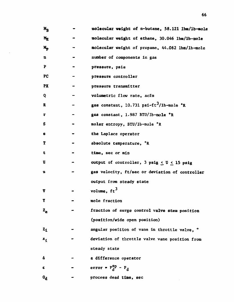
molecular weight of n-butane, 58.121 lbm/lb-mole

molecular weight of ethane, 30.046 lbm/lb-mole

molecular weight of propane, 44.062 lbm/lb-mole

number of components in gas

pressure, psia

pressure controller

pressure transmitter

volumetric flow rate, acfm

gas constant, 10.731 psi-ft^/lb-mole °R

gas constant, 1.987 BTU/lb-mole °R

molar entropy, BTU/lb-mole °R

the Laplace operator

absolute temperature, °R

time, sec or mln

output of controller, 3 psig U 15 psig

gas velocity, ft/sec or deviation of controller

output from steady state3volume, ft

mole fraction

fraction of surge control valve stem position

(position/wide open position)

angular position of vane in throttle valve, °

deviation of throttle valve vane position from

steady state

a difference operator

error - P^P - Pd

process dead time, sec

n - efficiency

p - specific density

t - process time constant, sec

- controller derivative time, sec

Y - proportionality constant

Subscripts and Superscripts

B - n-butane

c - refers to compressor or cooler

d - discharge

di - Isentropic discharge

E - ethane

e - refers to bypass loop

1 — inlet, isentropic

m - mlsture

o - outlet

P - propane

s - suction

ss - steady-state

v - valve

68

LITERATURE CITED

1. Brown, R. N., "Control Systems for Centrifugal Compressors," Chemical Engineering. (February 17, 1964), pp. 1 3 5 -1 3 8 .

2. Byrne, E. J., "Centrifugal Compressor Control Problems," Petroleum Chemical Engineer, (Mar. 1963), pp. 213-215.

3. Compressed Air and Gas Handbook, Third Edition (Revised 1966), Copyright 1961 by the Compressed Air and Gas Institute, 122 East 42nd Street, N. Y., N. Y.

4. Daze, R. E., "How to Instrument Centrifugal Compressors," Hydrocarbon Processing. (Oct. 1965), pp. 125-130.

5. Hancock, R., "Drivers, Controls and Accessories," Chemical Engineering, (June 1956) pp. 227-238.

6. Hicks, T. G., "Refrigeration In the Refining Industry", Petroleum Refiner, Part I, (Mar.1951), pp. 88-90, Part II, (June 1951), pp. 145-146.

7. Moens, J.P.C., "Adapt Process to Compressor," Hydrocarbon Processing, (Dec. 1971), pp. 96-100.

8. Tazekjian, E. A., "How to Control Centrifugal Compressors," Hydrocarbon Processing and Petroleum Refiner, (July 1963), pp.169-176.

9. Moore, R. W., "Allocating Pressure Drops to Control Valves," Instrumentation Technology. (Oct. 1970), pp. 102-105.

10. Emmons, H. W., Pearson, C. E. and Grant, H. P., "Compressor Surge and Stall Propagation," Transactions of the ASME, 77 (1965), pp. 455-469.

11. Instrument Engineers Handbook, Ed. B. G. Liptak, Chilton Book Co., N.Y., N. Y., 1969.

12. Chinn, G., "Sizing Butterfly Valves," Instruments and Control Systems, 38, (Mar. 1965), pp. 120-122,

13. Thinh, T. P., Duran, J. L., Ramalho, R. S. and Kaliaguine, S., "Equations Improve CS Predictions," Hydrocarbon Processing, (Jan. 1971), pp. 98-103.

69

14. Franks, R. G. E., Mathematical Modeling In Chemical Engineering. John Wiley and Sons, Inc., N.Y., N.Y., 1967.

15. Csanady, G. T., Theory of Turbomachines, McGraw-Hill Book Co., New York, 1964.

16. Fulleman, J., Chapter 8 of Advances in Petroleum Chemistry and Refining. Ed. McKetta, J.J., Jr., Interscience Publishers, N.Y., N.Y., 1962.

17. Shepherd, D. G., Principles of Turbomachinery. Macmillan Co., N.Y., N.Y., 1956.

18. Carnahan, B., Luther, H.A. and Wilkes, J.O., Applied Numerical Methods. John Wiley and Sons, Inc., New York, 1969, Chapter 3.

19. Bergeron, E. P., and Corripio, A. B., "Simulation of Start-Up of an Industrial Refrigeration System," Proceedings of the 1971 Computer Simulation Conference. Boston, Mass. (July 1971),pp. 306-315.

20. System/360 Continuous System Modeling Program (360 A-cx-16x). User's Manual (H20-0367-2), IBM Corporation, Data Processing Division, 112 East Post Road, White Plains, New York, 1968.

21. Sl-1 Reference Manual for XDS Sigma 5/7 Computers, Xerox Data Systems, Inc., 701 South Aviation Boulevard, El Segundo, California, May, 1970.

22. Harriot, P.., Process Control. McGraw-Hill Book Co., New York, 1964, Chap. 13.

23. Lopez, A. M., Miller, J. A., Murrill, P. W. and Smith, C. L., "Controller Tuning Relationships Based on Integral Performance Criteria," Instrumentation Technology. 14, No. 11 (Nov. 1967), p. 57.

24. Wilde, D. J., Optimum Seeking Methods, Prentice-Hall, Englewood Cliffs, N. J., 1964.

CHAPTER III

THE CONSTANT SPEED REAL GAS MODEL (CSRGM)

Introduction

In this chapter the concepts Introduced In the previous

chapter will be extended to account for the nonidealities of the

gas. This will be accomplished by incorporating into the CSIGM

the modified Benedlct-Webb-Rubin (MBWR) equation of state devel

oped by Starling [1]

P « CRT + (BqRT - A0 - C0/T2 + Dq /T3 - E0/T**)C23 6+ (bRT - a - 6/T)C + a(a +6/T)C

+ (cC3/T2)(l + y C2 ) exp (-yC2). III-l

Starling has reported the constants for the straight chain alkanes,

C1 through C&[2].

This particular equation of state was chosen because, accord

ing to Starling, it is exceptionally accurate for both the liquid

and vapor regions. This is a desirable trait because in many

applications the model of an entire process containing a compressor

will involve the liquid state. Also, all of the equations which

will subsequently be derived can be easily modified so that gases

other than methane, ethane, propane, n-butane, n-pentane, and

n-hexane can be handled. This is done by reducing Starling's

equation to the BWR equation of state by setting DQ , EQ and 6 to zero.

70

71

Another and the more Important reason the MBWR (or BWR) equa

tion of state has been chosen is that it is one of the most

complicated equations of state. A complicated equation of state

was desired so that both ends of the spectrum of complexity could

be examined so as to provide yardsticks for ascertaining degrees

of difficulty in programming, computer storage requirements, com

puter time requirements, etc. relative to desired accuracy. The

previous chapter examined the simplest case and this chapter will

examine the most complicated and the most accurate case. Any

models developed in terms of other equations of state, such as the

well known two constant Redlich-Kwong equation of state, should

fall somewhere, in terms of complexity, between the CSIGM and CSRGM.

Based upon the same physical system which was developed in

Chapter II, a detailed development of the changes necessary to

incorporate the MBWR into the constant speed centrifugal compressor

model will be presented. The resulting model is designated the

CSRGM and it will be summarized in terms of a table of dynamic

equations and an information flow diagram.

Open loop simulation results of the time response of the dis

charge pressure to step changes in inlet temperature and pressure

and in molecular weight of the gas will be presented in the form

of continuous curves. A comparison will be made between the open

loop CSRGM and CSIGM results in terms of a tabulation of the steady

state head, volumetric flow rate and discharge pressure and the

time required to reach these new steady states. The chapter will

be concluded with a closed Loop response analysis as was done

in Chapter II.

72

Mathematical Model

The principles presented in Chapter II upon which the devel

opment of the lumped parameter CSIGM was based will be utilized

to develop the CSRGM as it is also a lumped parameter model. Many

of the expressions derived as a part of the CSIGM will be unchanged

by the inclusion of the MBWR equation of state and hence will be

presented only in brief. However, those expressions which are

affected will be presented in detail.

Suction System

As in the CSIGM, the mathematical expressions required to

model the suction system are unsteady state energy and mass balances

and the standard valve equation. The mass balance is that given in

equation II-2

P8 - <*1 + - 0s(Jc^V9 “ -2

and the valve equation is that given in equation II-3 with slight

modification. The maximum valve flow factor, Cy^ has been adjusted

from 9541. lbm/min to 10174.lbm/min so that when the discharge

pressure control loop is closed the valve will operate at the same

steady state position as in the CSIGM. The other modification involves

the calculation of the inlet density when the inlet temperature and

pressure are known. Since the MBWR equation of state is implicit

In density, a trial and error Iterative procedure is required. The

procedure utilized is given in Appendix B. The valve equation uti

lized is

Fj - 1.05 x 10174. Cvi ^ 0 . 5 ^ + P g ) ^ - P ) . III-2

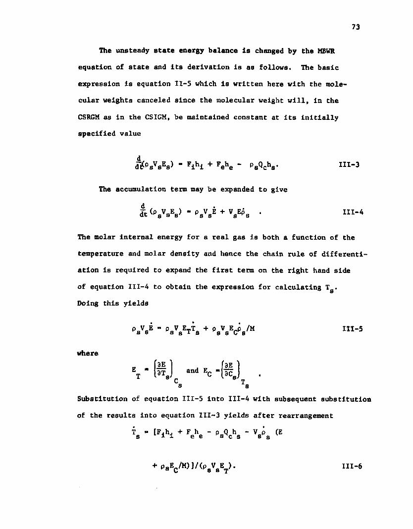
The unsteady state energy balance is changed by the MBWR

equation of state and Its derivation Is as follows. The basic

expression is equation II-5 which is written here with the mole

cular weights canceled since the molecular weight will, in the

CSRGM as in the CSIGM, be maintained constant at its initially

specified value

The molar internal energy for a real gas is both a function of the

temperature and molar density and hence the chain rule of differenti

ation is required to expand the first term on the right hand side

of equation III-4 to obtain the expression for calculating T .

Doing this yields

Substitution of equation III-5 into III-4 with subsequent substitution

of the results into equation III-3 yields after rearrangement

III-3

The accumulation term may be expanded to give

III-4

III-5

where

Ts s

+ p8sc/n>]/<p8v y . m - 6

74

In view of the fact that the Internal energy and the enthal

pies cannot be given absolutely, choose the bypass temperature Te

as the thermal datum plane. Then h = 0 and E„, h. and h can bee s ’ i sdetermined from the expressions given in Appendix D.

Writing equation D-25 with T = T , T_ 10 T and C ■ C ■ C.A e 0 i A B iyields the following expression for the inlet enthalpy relative to

the bypass temperature:

h± - {-(B0RTe - 4Cq /T* + 5Dq /T* - 6Eo/T*)C±

2 5-(bRTe - 26n e ) C ± - 1.4016(^/1,

2 2 2 2 -(c/yTe) [3-(3 + O.SyCj-y (^expC-yC^) ]

+(B0RT1 - 4Cq /T* + 5Dq /T* - b E ^ x J ) ^

2 5+(bRT± - 26/Ti)C1 + 1.4a6C1/Ti

+(c/yT^)[3 - (3 + 0.5yC^-y2C^)

exp 7 7 ^ 9 + 3* CTi ' Te>

+ (b*/2)(Ti2- T2) + ( c V s X T i 3- TI )

+ (d*/4) (Ti‘t- Tg) . III-7

If, in this expression, and are replaced respectively with

T and C , the following expression for evaluating the enthalpy of 8 S

the gas within the suction volume relative to the temperature of

the bypass gas is obtained:

hs - {-<B0RT, - 4C0/T* + 5DQ/Tg - 6E0/T*>C,

752 5

-(bRT - 26/T )C - I.A06C /Te 8 8 e

“ (c/yXg) [3- (3 + 0.5yC* -yV) exp (-YC J ]2 3 5

+ (B RT - 4C /T + 5D /T - 6E /T )CO S O S O S 0 8 8

2 5+ (bRT - 26/T )C + 1.4a6C /T

8 8 8 8 8

+ (c/yTj[3- (3 + 0.5yC* -yV) exp (8 S S

tTTS s + a‘(W + (b*/2><T8 - V+ (c*/3) (T^ - T J + (d*/4) (T** - T J . III-8s e s e

The expression for evaluating the internal energy of the gas

within the suction volume is obtained by writing equation D-38

with T. * T , T = T and C. ■ C_ ■ C . Doing this yields A e B 8 A B s ° J

2 3 kE - {- (3C /T - 4D /T + 5E /T ) C 8 0 8 0 8 0 8 8

2 5 2- 6C /T + 0.4ct6C /T + (3c/yT ) [18 8 8 8 8

- (1 + 0.5yCJ exp (-yCJ] + (3CJ ?o 8 0 63 4 2 5

- 4D /T + 5E /T )C + 6C /T - 0.4ct6C /To e o e s 9 e s e

-(3c/yTj[l - (1 + 0.5YCjexp(-yCj]} J A 4 *777.649

+(a*-r) (T -T ) + (b*/2)(/ - T J 8 6 8 6

+(c*/3) (T^ - T J + (d*/4)(T* - T J . III-9s e s e

Evaluation of the two partial derivatives results in3 4 5

E_ - {(6C /T - 12D /T + 20E /T )C T 0 8 O S 0 8 8

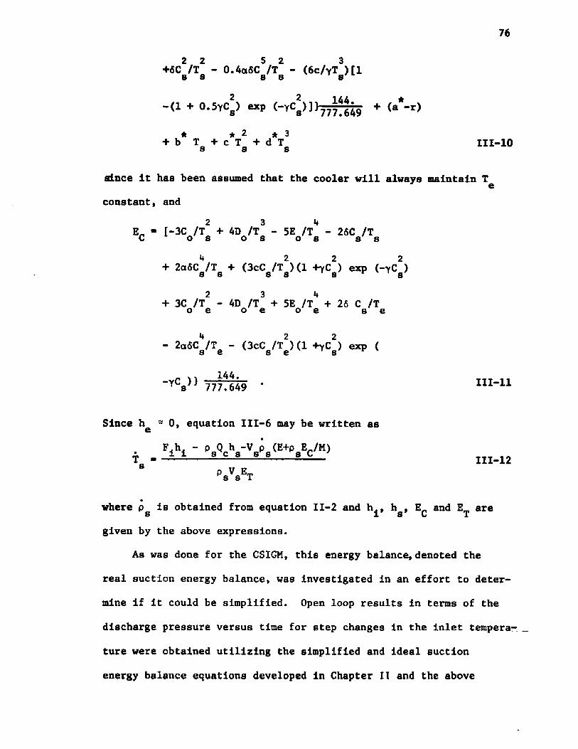
76

2 2 5 2 3+6C /T - 0.4o6C /T - (6c/yT )[1 8 8 8 8 8

-(1 + O.Sy c') exp < - Y C * > J + <a*-r>

* * 2 -ft 3+ b T + c T + d T III-IO8 8 8

since It has been assumed that the cooler will always maintain

constant, and2 3 h

E_ - [-3C /T + 4D /T - 5E /T - 26C /T C o s O S 0 8 8 84 2 2 2

+ 2a6C /T + (3cC /T ) (1 +yC ) exp (-yC )8 8 8 8 8 82 3 4

+ 3C /T - 4D /T + 5E /T + 26 C /T o e o e o e s e

- 2a6C%T - (3cC /T J (1 +yC J exp (o 6 8 6 S

144"yCs )} 777.649 * III-ll

Since h^ - 0, equation III-6 may be written as

. Fihi - > . i . V V . < ,t<l. V ll>

-

where p is obtained from equation II-2 and h., h , E_ and E are 8 1 8 L Tgiven by the above expressions.

As was done for the CSIGM, this energy balance, denoted the

real suction energy balance, was Investigated in an effort to deter

mine if it could be simplified. Open loop results in terms of the

discharge pressure versus time for step changes in the inlet tempera

ture were obtained utilizing the simplified and ideal suction

energy balance equations developed in Chapter IT and the above

77

equation. The results are shown in Figure III-3 and it is apparent

from them that the suction energy balance could have been derived

based upon the assumption that the gas is an ideal one with constant

heat capacity. This assumption is valid only because of the small

temperature difference at the suction since utilization of the ideal

gas law rather than equation III-l as the suction equation of state

does introduce significant errors.

Discharge System

The equations required to model the discharge system are exactly

the same as those given in Chapter II. As a result they will not be

given here but will subsequently be given in the summation of the

CSRGM dynamic equations.

Compressor

The concepts presented in Chapter II relative to modeling the

compressor proper are not changed when the nonidealities of the gas

are accounted for by the introduction of the equation of state of a

real gas. The basic equation is still a steady state energy balance

H - 778. Ah/M. 11-21

The H-Qc curve is the same as that shown in Figure II-4 and its

equation is the same as that given in equation 11-24

H - H » A(Q - Q ) 2 . II-24m c mThe steps required to calculate the volumetric flow rate through the

compressor remain unchanged and are

1. Isentropic entropy balance to obtain the isentropic

discharge temperature t ^

78

2. Calculation of the Isentropic enthalpy change

utilizing the suction temperature and density and

the discharge density and

3. Calculation of the actual enthalpy change based on

the efficiency of the machine and the isentropic

enthalpy change

and4. Calculation of the volumetric flow rate utilizing

equation 11-30

Q = 0 + /(H - 777.649 Ah/M)/(-A). 11-30C m I D

However, the expressions required to perform these steps as well

as the expression required to calculate the actual discharge tempera

ture are changed considerably from those presented in Chapter II

and will be presented here based on the thermodynamic derivations

given in Appendix D.

For the isentropic or reversible compression of the real gas

represented by the MBWR equation of state, from the suction conditions

of Tg and Cg to the discharge conditions of and C^, equation D-10

is applicable with AS ■ 0, C. ■ C , T. ■ T , C_ = C, and T„ * T,..r r A s A s B d B di

After making these substitutions, equation D-10 may be expanded to3 b 50 - {C (B R + 2C /T - 3D /T + 4E /T )S O 0 8 O S O S

2 2 5 2+ 0.5 C (bR + 6/T ) - 0.2a<5C /T S S s s

-(2c/yTj[l - (1 + 0.5 yCj] exp (-yCjJ - C,(BR s s 8 a o

5 2 3 2+ 0 . 2 oSCd/Tdl + (2c/YTdl)[l - (1 + 0.5yCd) exp (

2 144 *"YCd)]} 777.649 + “ r) *n (Tdi/Ts) “ r *nCd/Cs

+ *>*(Tdl -Tg) + (c*/2) (Tdl - Tg) + (d*/3)(Tdl-Tg) . 111-13

The only unknown In this expression Is the isentropic discharge

temperature Tdi which may be obtained through the use of the impli

cit function solving routine. The routine used is Newton's, the

same as that used in the CSIGM, and the required equations are given

in Appendix B.

The enthalpy change Ah^ associated with this isentropic compres

sion is obtained from equation D-25 after making the same substitu

tions as those given above. Expansion of equation D-25 after makingthese substitutions yields 2 3 t+

Ah. « {C,(B RT,, - 2A - 4C /T.. + 5D /T,, - 6E /T..) i d o di o o di o di o di'2 5

+ <bRTdi - 1.5a - 26/Tdi)Cd + 0.2a(6a+76/Tdl)Cd

+ (c/yTdi)[3-(3 + 0.5yCd -yVj) exp (-yC*)]

2 3 1+-[C (B RT - 2A - 4C /T + 5D /T - 6E /T )

S O S O O S O S 0 8

2 5+(bRT - 1.5a - 26/T )C + 0.2a(6a + 76/T )C s s s s s

+<c/y/)[3- (3 + O.SyC* -yV> exp <-yC*) ] J+a*(Tdl - Tg) + (b*/2)(Tdi-Tg) + (c*/3)(Tdl-Tg)

+(d*/4)(Tdl - Tg). 111-14

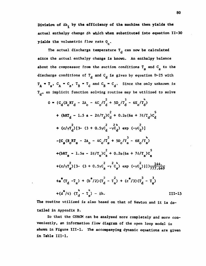
80

Division of Ah^ by the efficiency of the machine then yields the

actual enthalpy change Ah which when substituted into equation 11-30

yields the volumetric flow rate Q^.

The actual discharge temperature T, can now be calculateddsince the actual enthalpy change is known. An enthalpy balance

about the compressor from the suction conditions T and C to the8 8

discharge conditions of and is given by equation D-25 with

T. ■ T , C. ■ C , T_ ■ T, and C„ ■ C,. Since the only unknown is A s A s B d B d J

T^, an implicit function solving routine may be utilized to solve2 3 4

0 - {C.(B RT. - 2A - 4C /T. + 5D /T. - 6E /T.) d o d o o d o d o d2 5

+ (bRTd - 1.5 a - 26/Td)Cd + 0.2a(6a + 76/Td>Cd

+ (c/yTd)[3- (3 + 0.5yCd -yC*) exp (-yC*)]

2 3 4- r c (B RT - 2A - 4C /T + 5D /T - 6E /T )* 8 0 8 0 O S O S O S

2 5+(bRT - 1.5a - 26/T )C + 0.2a(6a + 76/T )C 8 8 8 8 8

2 2 2 4 2 16a+(c/YTs)[3- (3 + 0.5yCe -y Cg> exp C -y C ,)]]

+a*(T. -T ) + (b*/2)(Tj - TJ + (c*/3)(t! - TJ a s a s a s* 4 4+(d /4) (T. - T ) - Ah. 111-15a s

The routine utilized is also based on that of Newton and it is de

tailed in Appendix B.So that the CSRGM can be analysed more completely and more con

veniently, an Information flow diagram of the open loop model is shown in Figure III-l. The accompanying dynamic equations are given in Table III-l.

Eqn. 10 Eqn. 1 Eqn. 2

Eqn. 13

Eqn. 4nEqn. 3r m■p I s_

eQ,

Eqn. 15 Eqn. 16Ive Eqn. 23

Fe Eqn. 19 or 20Ah1 Eqn. 27

AhEqn. 30

Ah

9 -

Ahi n — — I Eqn.LCd i Ts26

I — 5------ Td . pd ,Eqn. 28 Eqn. 24 Eqn. 18

d l Eqn. 25 Tdt * {

Cd

Figure III-l. Information Flow Diagram for Open Loop CSRGM.

82

Suction System

Mass balance

Molar density

Energy balance

Inlet density

Inletenthalpy

Suctionenthalpy

TABLE III-l

CSRGM DYNAMIC EQUATIONS

Ps ’ ("i + Fe - ‘>s9c)/Vs (1)

Cs - Pj/M (2)

• . Fihi - "A h. ' V P +8 P v E_s s T

0 - C.RT. + (B RT4 -A -C / T j 1 1 o 1 o o i3 4 2+ D /T - E /T ) C + (bRT.0 1 O i l 1

3 6- a - 6/T±)C± + a(a + 6/T )C

cC 2+ - T - (1 + YC1)exp(-YCi) - P± (A)

Ti

\ “ { [hiCy-hjCr ] + c [h2(T h2CTe)]+ c^fha^J-hgd^] + hk(T1#c±)

1LL- M T g . c p } 7777649 + hid(Ti) " hid^Te^

ha “ tc8th l < V _hl(Te)] + Csfh2<T8>-h2<Te)]

+ C8[h3(Ts)-h3(Te)] + hlt(Ts,Cs)

“ M Te »csH 777.6A9 + hid*Ta*”hid*Te*

83

Suction energy

Energy change with temperature

Energy change with composition

Inlet mass rate

TABLE III-l (Cont'd)


! - iCaIEj<Te)-Ei(Ta)J + C26[l/Te-1/T8)[l-

0.4aC ] + E2(T ,C ) - E2(T .C )} 14A*s' s' s e* s 777.649

+ h±d(Ts) - hid(Tfi) -r[T8-Te] (7)

"T ' (H-j " tCa[6Ca/Ts ' 12 Do/Ts8 c8

+ 20 E /T5] + 6C2 [1 - 0.4oC3]/T20 8 S 8 8

- 2 E2<Ts,C8)/I8) + (a*-r)

+ b*T + c*T2 + d*T3 (8)S 8 S ' '

- [|§-] - {E,(Tc)-E,(Tb) + 2«C8 I1/Ta8 T8

3 2-1/T ] [1-aC ] + 3cC (1 + yC ) exp(8 8 8 8

-YC8)(1/T8 - 1/T*]} (9)

1.05 C . ip ,AP . vl vi vi (10)

84

Throttle valve density

Throttle valve pressure drop

Throttle valve flow factor

Equation of state



pyi - 0.5 (ps + CtM) (11)

AP - P - P (12)vl 1 s

Cvi “ Cvi f(Zl) (*8ee below) (13)

2P - C RT + (B RT - A - C /T S 8 8 0 8 o 0 8

3 k Z+ D /T - E /T ) C + (bRT 0 8 0 8 8 8

3 6- a - 6/T )C + a(a+5/T )C 8 8 8 8

cC 2. 2+ tZ2, (1 +yC ) exp(-YC ) (14)

TS 8 8

*f(Z^) is the function which relates the fraction of the design Cv (expected maximum valve capacity) to the throttle valve vane position. It Is shown In Figure II-3.

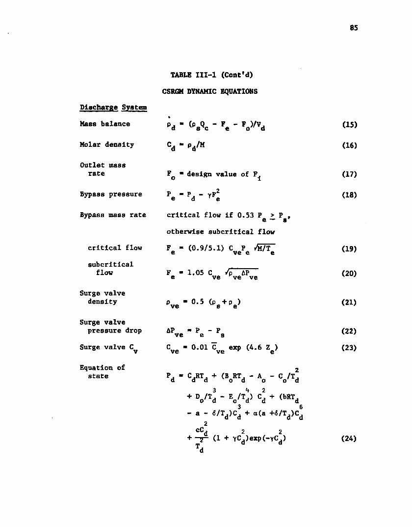
85

Discharge System

Mass balance

Molar density



Pd " (psQc - Fe “ Po)/Vd

Cd “ Pd/M

(15)

(16)

Outlet mass rate

Bypass pressure

Fq ■ design value of F^

P ■ P. - yFe d ' e

(17)

(18)

Bypass mass rate

critical flow

subcriticalflow

Surge valve density

critical flow if 0.53 P > P ,e — sotherwise subcritical flow

F - (0.9/5.1) C P /firr e ve e e

F - 1.05 C / p & P e ve ve ve

p ■ 0.5 (p +p ) ve 8 e

(19)

(20)

(21)Surge valve pressure drop

Surge valve C

AP - P - P ve e sC ■ 0.01 C exp (4.6 Z ) ve ve r ' e

(22)(23)

Equation of state CdRTd + (BoRTd “ Ao - Co/Td

+ 0,/T* - Eo/T^) C* + (bRTd3 6- a - 6/Tj)Cd + a(a +6/Td)Cd

2cC.

(1 + yCd)exp(-yCd) (24)

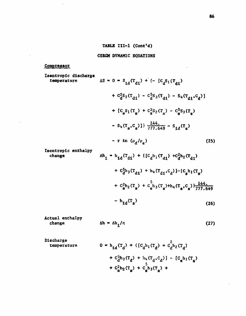
86

CompresBor

Isentroplc discharge temperature

Isentroplc enthalpy change

Actual enthalpy change

Dischargetemperature



AS - 0 - Sld(Tdl) + {- [CdSl(Tdl)

+ CdS2<Td i> - CdS3<Tdi> - S-<Td l*Cd »

+ [caSi(Ts) + c2s2(Te) - c|s3(tb)

- s- < V ce> J » 7 & - si d < V

- r in (Pd /P8) (25)

ihl - hid(Tdl> + t[Cdhl(Tdl>

+ Cdh3(Tdi) + h'*(Tdi'Cd)]*|Cehl<V+ c3h2(is) + c*h,(T8)dm(*B,cB))J44{j5

" hid(V (26)

Ah - Ah±/n (27)

0 ’ hld(V + (tCdhl(Id> + Cdh2<Td>+ Cjh3(Td) + M T d,Cd )J - tC8h!(T8)

+ Ceh2<IB) + C8h 3(T8) +

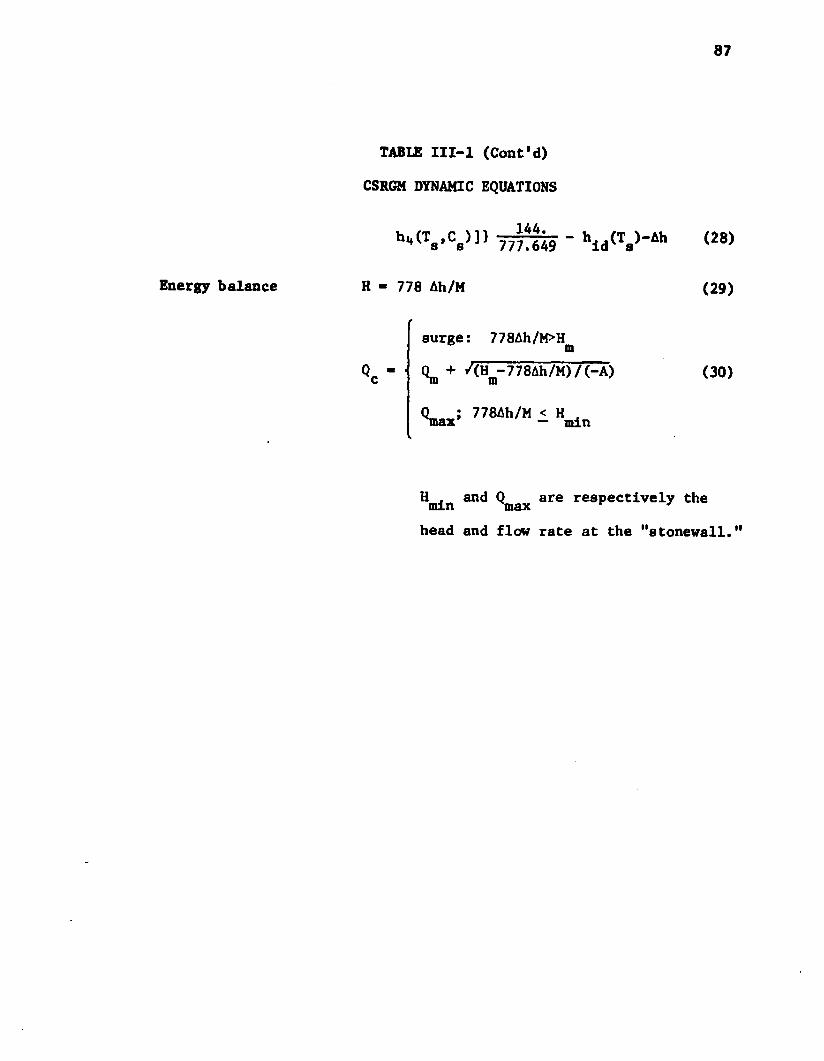
87

Energy balance



h -(V C»)]) 777^649 * hld(V _Ah <*»

H - 778 Ah/M (29)

Qc

surge: 778Ah/M>Hm+ /(Hn-7784h/M)/(-A) (30)

U ’ 7784h/M i v „

^min Qmax are respectively the head and flow rate at the "stonewall."

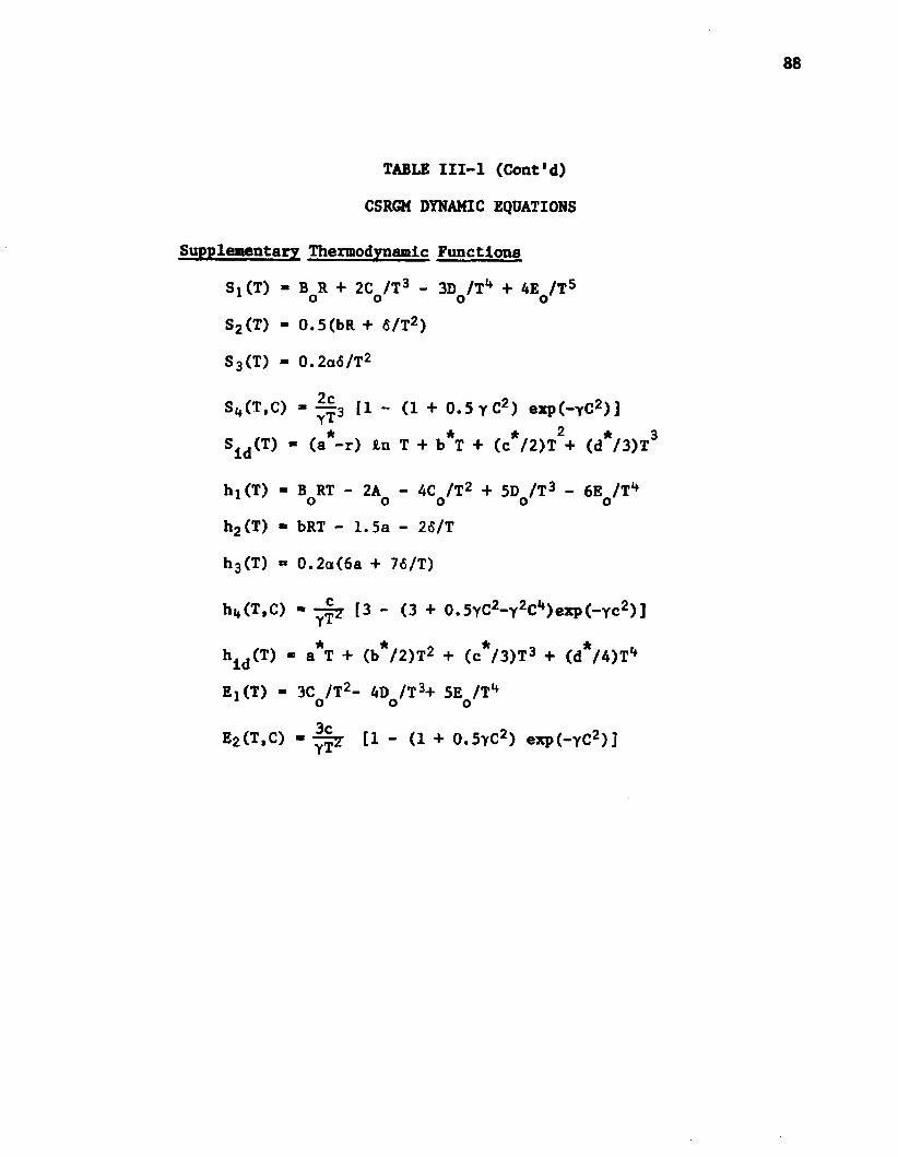
88



Supplementary Thermodynamic Functions

Si(T) - B R + 2C /T3 - 3D /Tu + 4E /T5 o o o oS2(T) - 0.5(bR + 6/T2)

S3(T) - 0.2a6/T2

S4(T,C) - i£3 [1 - (1 + 0.5 Y C 2) exp(-yC2)]

Sld(T) “ (a*-r) Jtn T + b*T + (c*/2)T2+ (d*/3)T3

hj(T) - B RT - 2A - 4C /T2 + 5D /T3 - 6E /T*» o o o o oh2 (T) - bRT - 1.5a - 26/T

h3(T) » 0.2a(6a + 76/T)

M T . C ) - [3 - (3 + 0.5YC2-y2Cl')exp(-yc2)]

hld(T) - a*T + (b*/2)T2 + (c*/3)T3 + (d*/4)T,f

E,(T) - 3C /T2- AD /T3+ 5E /T1* o o o

E2(T,C) - [1 - (1 + 0.5yC2) exp(-yC2)]

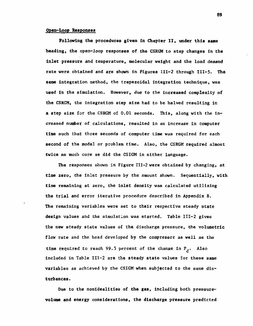
89

Open-Loop Responses

Following the procedures given in Chapter II, under this same

heading, the open-loop responses of the CSRGM to step changes in the

inlet pressure and temperature, molecular weight and the load demand

rate were obtained and are shown in Figures III-2 through III-5. The

same Integration method, the trapezoidal integration technique, was

used in the simulation. However, due to the increased complexity of

the CSRGM, the integration step size had to be halved resulting in

a step size for the CSRGM of 0.01 seconds. This, along with the in

creased number of calculations, resulted in an Increase in computer

time such that three seconds of computer time was required for each

second of the model or problem time. Also, the CSRGM required almost

twice as much core as did the CSIGM in either language.

The responses shown in Figure III-2 were obtained by changing, at

time zero, the inlet pressure by the amount shown. Sequentially, with

time remaining at zero, the inlet density was calculated utilizing

the trial and error iterative procedure described in Appendix B.

The remaining variables were set to their respective steady state

design values and the simulation was started. Table III-2 gives

the new steady state values of the discharge pressure, the volumetric

flow rate and the head developed by the compressor as well as the

time required to reach 99.5 percent of the change in P^. Also Included in Table III-2 are the steady state values for these same

variables as achieved by the CSIGM when subjected to the same dis

turbances.

Due to the nonidealities of the gas, including both pressure-

volume and energy considerations, the discharge pressure predicted

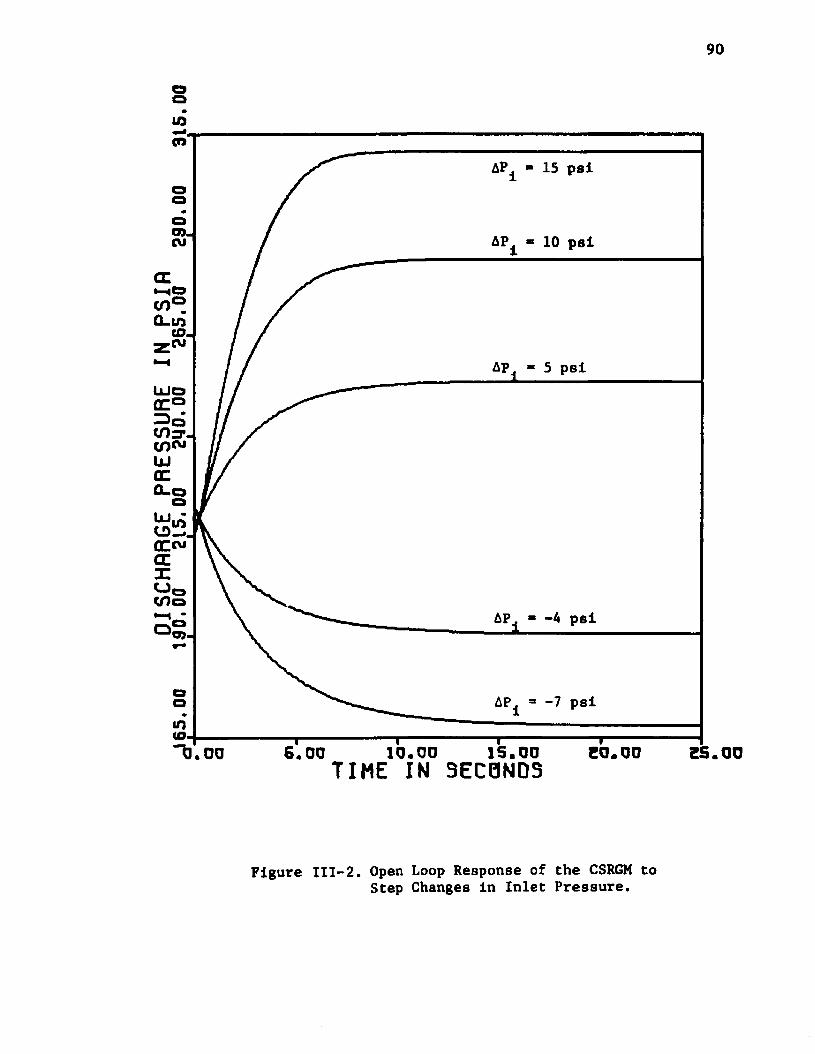
90

U3co

15 psl

05.CM AP 10 psl

CO .CL 10 10.

r r C ”

5 psl

-4 pslAP05-

-7 psl

to .

1 5 . 0 010 .0000 T I M E IN SECONDS

Figure III-2. Open Loop Response of the CSRGM toStep Changes in Inlet Pressure.

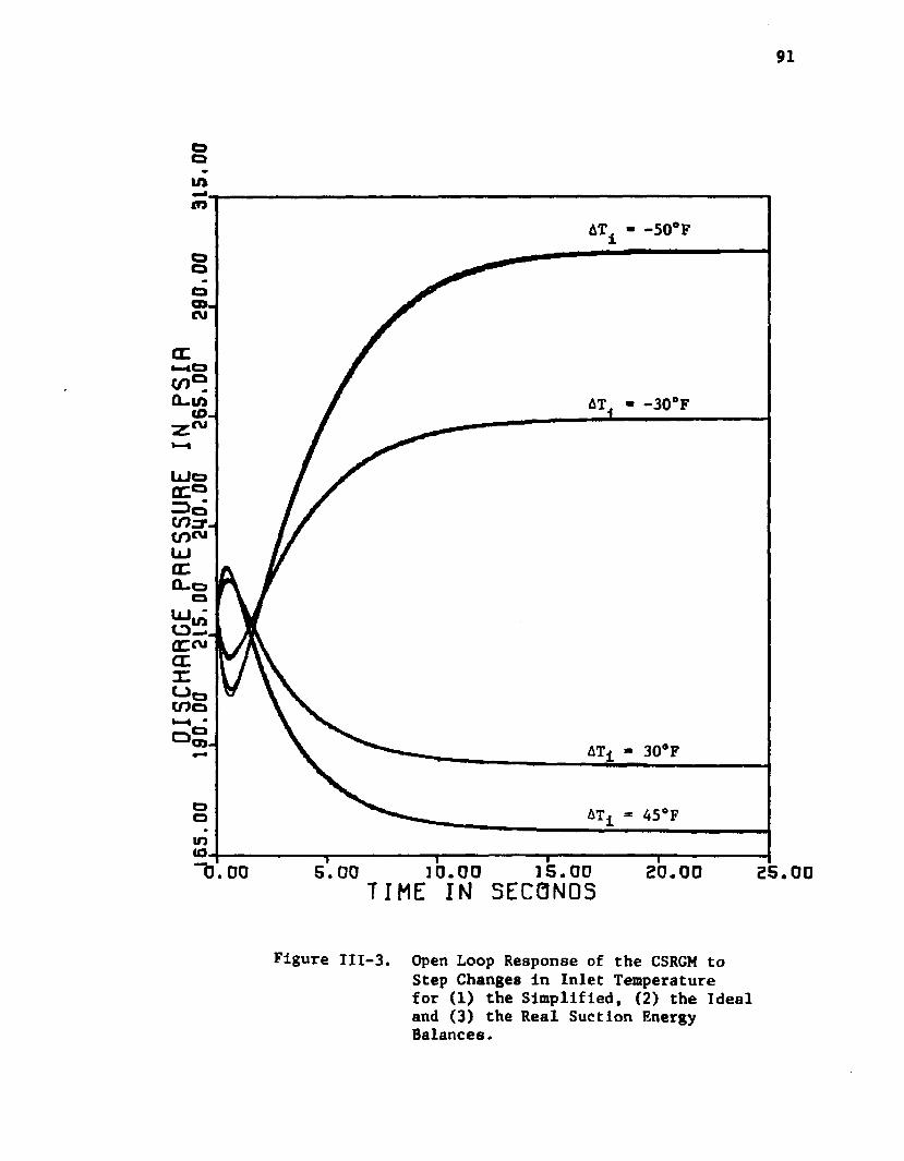
91

into

AT

axCM

*—iATj « 30°F

ATinto

15.005.00 1 0 .0 0 20.00 25.00TIME IN SECONDSFigure II1-3. Open Loop Response of the CSRGM to

Step Changes In Inlet Temperature for (1) the Simplified, (2) the Ideal and (3) the Real Suction Energy Balances.

DISC

HARG

E PR

ESSU

RE

IN PS

IA.1

80.0

0 20

0.00

22

0.00

24

0.00

26

0.00

28

0.00

30

0.00

I I I

l I

I l

I

92

AM ** 3 lbm/lb-mole

AM ■ 2 lbm/lb-mole

AM ■ 1 lbm/lb-mole

AM ■ -1 lbm/lb-mole

AM=-1.95 lbm/lb-mole

5. OC 15. CO10.00TIME IN SECONDSFigure III-4. Open Loop Response of the CSRGM

to Step Changes in Molecular Weightof the Gas.

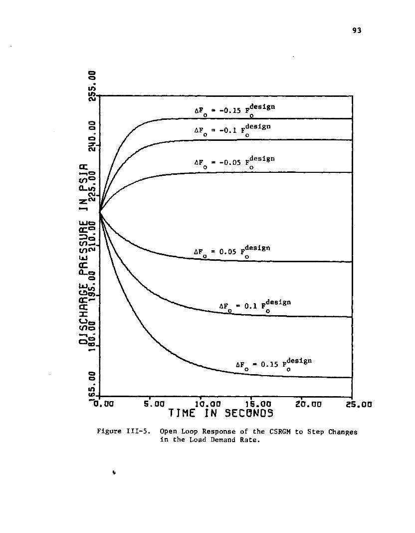
93

ID.CM-0.15 Fdesign

.designo

CM.design

0.05 FdealgnAFa :Q_o

.designAF

CO.

0.15 Pde8l6"AF

into0.00 S. 00 20.0015.0010.00TIME IN SECONDSFigure III-5. Open Loop Response of the CSRGM to Step Changes

in the Load Demand Rate.

TABLE III-2. OPEN LOOP COMPARISON OF CSRGM WITH CSIGM

Disturbance P88 (psia) tc (second) H88 (ft-lbf/lbm) Q88 (acfs)

CSRGM CSIGM CSRGM CSIGM CSRGM CSIGM CSRGM CSIGMAP ■ 15 psi

1 10 "5 "

-4 " -7 n -8 "

310.77 283.81 253.58190.78 167.67 surge

293.75272.44247.97194.91174.53167.46

7.89.8 12. 15.7 16.3 surge

5.57.29.012.913.814.1

21736.21461.20838.18331.16891.surge

21662.21342.20736.18506.17270.16783.

240.53257.12275.92316.94333.31surge

246.86261.61278.3314.74329.26334.43

AT - 50 °F 48.5" 30 "

-30 " -50 "

surge167.19185.33264.21302.51

181.31184.97196.22245.38263.12

surge14.6 15.015.7 16.6

14.014.0 13.8 11.6 10.7

surge16661.17972.20980.21513.

17542.17797.18513.20649.21111.

surge335.69321.3272.4 254.88

326.26323.34314.64280.22268.85

AM - 3 lbro/mole 2 1

-1-1.95 "-2 "

267.69250.8 234.96 205.83192.9 surge

251.43241.00230.50209.45199.39198.86

17.716.7 15.3 14.113.8 8 urge

10.410.7 11.011.511.711.7

20973.20635.20220.19133.18475.surge

20749.20460.20120.19261.18751.17723.

272.58280.53288.8306.3315.13surge

278.00284.17290.63304.46311.54311.92

AF— -- — 0.15p design ^0 -0.05

0.05 0.1 0.15

248.25241.73232.22205.36188.77170.66

246.06240.08231.32206.3190.58173.26

6.79.111.815.617.117.9

5.07.0 8.512.514.6 15.5

216222123620606185711713715400

216142122420597185911718515491

249.35265.14281.15 313.89 330.7 347.87

249.84265.5281.34313.64330.19347.03

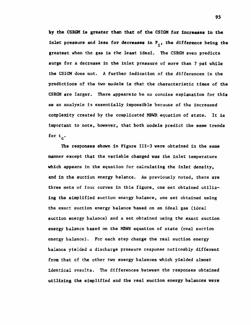
95

by the CSRGM is greater than that of the CSIGM for Increases in the

inlet pressure and less for decreases in P^, the difference being the

greatest when the gas is the least ideal. The CSRGM even predicts

surge for a decrease in the inlet pressure of more than 7 psi while

the CSIGM does not. A further indication of the differences in the

predictions of the two models is that the characteristic times of the

CSRGM are larger. There appearsto be no concise explanation for this

as an analysis is essentially impossible because of the increased

complexity created by the complicated MBWR equation of state. It is

Important to note, however, that both models predict the same trends

for t .cThe responses shown in Figure III-3 were obtained in the same

manner except that the variable changed was the inlet temperature

which appears in the equation for calculating the inlet density,

and in the suction energy balance. As previously noted, there are

three sets of four curves in this figure, one set obtained utiliz

ing the simplified suction energy balance, one set obtained using

the exact suction energy balance based on an ideal gas (ideal

suction energy balance) and a set obtained using the exact suction

energy balance based on the MBWR equation of state (real suction

energy balance). For each step change the real suction energy

balance yielded a discharge pressure response noticeably different

from that of the other two energy balances which yielded almost

identical results. The differences between the responses obtained

utilizing the simplified and the real suction energy balances were

96

deemed Insignificant and the former was utilized In the remainder

of the CSRGM simulations.

As in the above case, the characteristic time and the steady

state value of P., Q and R have been included in Table III-2 for a cboth the CSRGM and CSIGM. A point of major Interest Is that the

CSRGM predicts an increasing t while the CSIGM predicts just the

opposite as AT^ is varied from a maximum positive to a maximum

negative value though the tc 's tend to the same values as surge is

approached. There does not appear to be any simple explanation for

this other than the system time constant predicted by the CSRGM is

more strongly dependent upon factors which have been introduced by

the real gas equation of state than it is on Q . Note that bothcQ trends are the same, c

The responses shown in Figure III-A were obtained as in

Chapter II by instantaneously replacing the pure propane contained

within the system with a mixture of propane and ethane for the

negative AM's and a mixture of propane and n-butane for the positive

AM's. This replacement of the pure propane was accomplished by

specifying either a n-butane mole fraction with the ethane mole

fraction set to zero or an ethane mole fraction with the the n-butane

mole fraction set to zero. In addition to equations 11-33 through

11-38 which were used to calculate the new mole fraction of propane,

the new molecular weight and the new heat capacity constants, the

following equations as specified by Benedict, etal [3] were used to

calculate the new constants of the equation of state:

where the summations are for all the components.

These results have been included so that any differences between

the predictions of the two models for gases other than propane could

be examined. As in the AT. case, there is a reversal in the t trendsi cwith an apparent convergence to the same t as surge is approached.

The explanation given for the At^ case must hold here also. A point

worthy of mention is that the CSRGM predicts surge for any ethane

concentration greater than 13.9 mole per cent while the ethane con

centration for which the CSIGM predicts surge is 40 mole per cent

and greater.

The responses shown in Figures III-5 were obtained by perturbing

the load demand rate as was done in Chapter II. Note that the dyna

mics exhibited by these responses are essentially the same as those

predicted by the CSIGM. Table III-2 indicates that the new steady

state values of discharge pressure as predicted by each model are

the same. Thus, it is apparent that if a compressor study is to be

undertaken which entails ascertaining the effects of load demand rate

changes on proposed control schemes, the simpler CSIGM would be the

preferred model.

Closed-Loo£ Results

As a continuation of the analysis of the CSRGM, the discharge

pressure control loop was closed with the same pneumatic control

98

system as was utilized in the dosed loop analysis of the CSIGM.

Following the same procedure as was presented In Chapter II, eight

process reaction curves for the range -1.4 £ AU^ j< 1.4 were deter

mined utilizing the CSRGM. These curves along with the necessary

geometrical construction for obtaining the system gain K, time

constant t and dead time 0^ are shown in Appendix C. The results

of these process reaction curves are tabulated in Table III-3 and

the extrapolated curves for determining K, t and 0^ for zero step

change in the controller output are shown in Figures III-6,

III-7 and III-8 respectively. The extrapolated values are K -

13.6 psi/°, t = 5.44 seconds and 0^ * 1.1 seconds, which differ from

the CSIGM values of K - 11.2 psi/°, t = 4.84 seconds and Q , ■ 0.87dseconds. A comparison of these three curves with those of the CSIGM

reveals a significant point. Even though the system parameters of

the CSRGM are the larger, the two sets of curves have almost the

exact same shape indicating that over the range considered no addi

tional nonllnearltles of an extreme nature have been Introduced.

The above values of K, t and 0, were substituted into the IAEaformula of Lopez and the following controller parameters were

obtained:

PID or PI or3-mode controller 2-mode controller

K - 0.32 K - 0.22c c

k r - 0.131 - 0.175

Td " 0.44

Each of these parameters is smaller than the respective parameters

of the CSIGM except for t , because of the Increased K, t and ()..a d

99

TABLE III-3. PROCESS REACTION CURVE RESULTS

U1(psig)

4Ui(V uiB)

*Pd(pd-pdS)

K

(iV sui>T

(sec.)°d(sec.)

14.9 1.4 14.37 10.26 4.81 1.02

14.5 1.0 10.73 10.73 4.93 1.

14.0 0.5 5.88 11.76 5.1 1.05

13.75 0.25 3.12 12.48 5.17 1.08

13.25 -0.25 -3.89 15.56 5.72 1.14

13.0 -0.5 -8.76 17.52 5.96 1.22

12.5 -1.0 -21.42 21.42 6.42 1.36

12.1 -1.4 -35.63 25.45 7.05 1.38

i

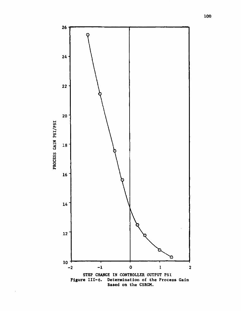
PROCESS

GAIN

PSI/

PSI

100

2 4 -

22 -

20 *

16 '

14 ‘

12 ‘

0 11-2STEP CHANGE IN CONTROLLER OUTPUT PSI

Figure III-6. Determination of the Process Gain Based on the CSRGM.

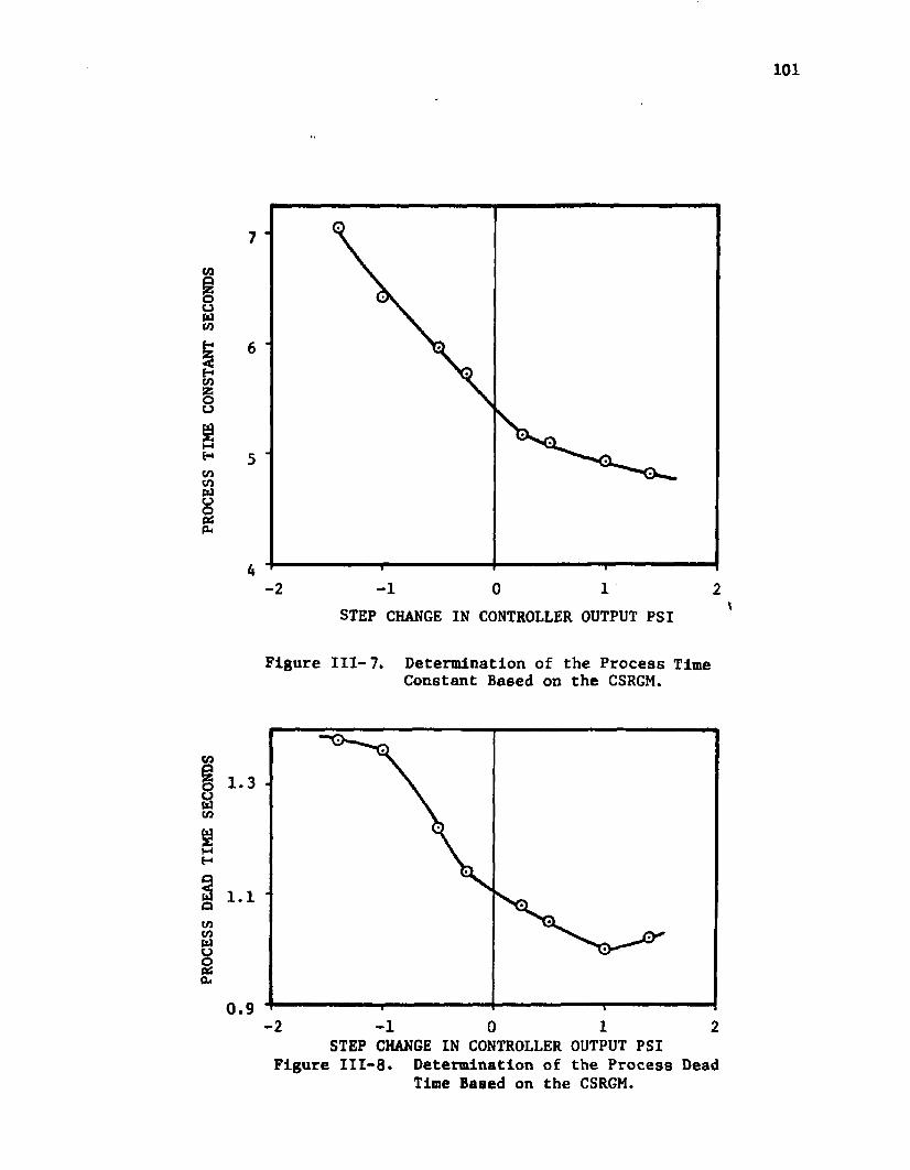
PROCESS

DEAD

TIME

SECONDS

PROCESS

TIME

CONSTANT

SECO

NDS

7

6

5

42 -1 0 1 2

STEP CHANGE IN CONTROLLER OUTPUT PSI

Figure III-7. Determination of the Process Time Constant Based on the CSRGM.

0.9-2 -1 0 1 2

STEP CHANGE IN CONTROLLER OUTPUT PSI Figure III-8. Determination of the Process Dead

Time Based on the CSRGM.

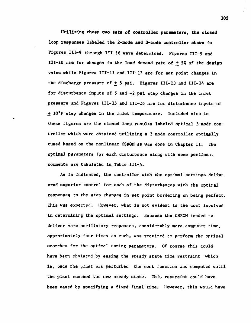
Utilizing these two sets of controller parameters, the closed

loop responses labeled the 2-mode and 3-mode controller shown In

Figures III-9 through III-16 were determined. Figures III-9 andIII-10 are for changes In the load demand rate of + 51 of the design

value while Figures III-ll and 111-12 are for set point changes in

the discharge pressure of + 5 psl. Figures 111-13 and 111-14 are

for disturbance inputs of 5 and -2 psl step changes in the inlet

pressure and Figures 111-15 and 111-16 are for disturbance inputs of

+ 10°F step changes in the inlet temperature. Included also in

these figures are the closed loop results labeled optimal 3-mode con

troller which were obtained utilizing a 3-mode controller optimally

tuned based on the nonlinear CSRGM as was done in Chapter II. The

optimal parameters for each disturbance along with some pertinent

comments are tabulated in Table III-4.

As is indicated, the controller with the optimal settings deliv

ered superior control for each of the disturbances with the optimal

responses to the step changes in set point bordering on being perfect.

This was expected. However, what is not evident is the cost involved

in determining the optimal settings. Because the CSRGM tended to

deliver more oscillatory responses, considerably more computer time,

approximately four times as much, was required to perform the optimal

searches for the optimal tuning parameters. Of course this could

have been obviated by easing the steady state time restraint which

is, once the plant was perturbed the cost function was computed until

the plant reached the new steady state. This restraint could have

been eased by specifying a fixed final time. However, this would have

103

effected the optimal parameters somewhat and would alao have clouded the comparison of the two models.

OISC

HRRG

E PR

ESSU

RE

JN PS

IR

,216

.00

216.

00

220.

00

222.

00

22U

.00

226.

00

226.

00U

i i

i i

a i

i

104

3-Mode Controller

Optimal (ISE) 3-Mode Controller

2-Mode ControllerOptimal (IAE) 3-Mode Controller

5. 00 15.0010.00 20.00 25.00TIME IN SECONDSFigure II1-9. Closed-loop Response of the CSRGM to 5%

Decrease in Load Demand Rate.

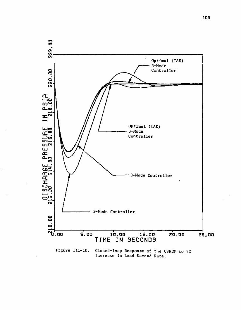
DISC

HARG

E PR

ESSU

RE

IN PSI

fl10

.00

212.

00

2U.0

0 21

6.00

21

6.00

22

0.00

22

2.00

105

Optimal (ISE)3-ModeController

Optimal (IAE) 3-Mode Controller

3-Mode Controller

2-Mode Controller

5. DODO 10.00 25.00TIME IN SECONDSFigure III-10. Closed-loop Response of the CSRGM to 5%

Increase in Load Demand Rate.

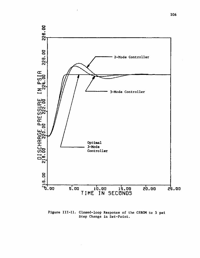
DISC

HRRG

E PR

ESSU

RE

IN PS

IR16

.00

216.

00

220.

00

222.

00

224.

00

226.

00

226.

00

106

2-Mode Controller

3-Mode Controller


5.00DO 25.0010 .00 20.00TIME IN SECONDS

Figure III-ll. Closed-loop Response of the CSRGM to 5 psiStep Change in Set-Point.

DISC

HRRG

E PR

ESSU

RE

IN PS

IR

10.0

0 21

2.00

214,

00

216.

00

216.

00

220.

00

222.

00

107


3-Mode Controller

2-Mode Controller

5.00 15. UO1 0 .0 000 25.00TIME IN S EC ONDSFigure III-12. Closed-loop Response of the CSRGM to -5 psi

Step Change In Set-Point.

DISC

HRRG

E PR

ESSU

RE

IN PS

IR12

.00

216.

00

220.

00

224.

00

226.

00

232.

00

236.

00

108

3-Mode Controller

Optimal 3-Mode Controller

2-Mode Controller

15.00 25.005. OO 1 0 . 0 0.00 TIME IN SECONDSFigure 111-13. Closed-loop Response of the CSRGM to 5 psl

Step Change In Inlet Pressure.

DISC

HARG

E PR

ESSU

RE

IN PS

IR12

.00

21M

.00

216.

00

216.

00

220.

00

222.

00

22U

.00

109


2-Mode Controller

3-Mode Controller

15.00 25.005.00 10.00. 00 t i m e i n s e c o n d s

Figure 111-14. Closed-loop Response of the CSRGM to -2 psiStep Change In Inlet Pressure.

110

CDru.cvi

Optimal3-ModeControllerC L

3-Mode Controller

cu2-Mode Controller

ID

SO.00DO 1 0 . 0 0TIME IN S EC O N D S

Figure 111-15, Closed-loop Response of the CSRGM to -10°FStep Change in Inlet Temperature.

Ill

o

CM.CM

CMCM.CM


CE

Q_o

3-Mode Controller

2-Mode ControllerO

CM

aoj

30.00o a 10 .00 50.00TIME IN SECONDSFigure 111-16. Closed-loop Response of the CSRGM to 10°F

Step Change in Inlet Temperature.

TABLE III-4. CLOSED LOOP CSRGM OPTIMIZATION RESULTS

Disturbance Kc ** Td Comments

AF * 5% o 0.50.35

0.10.15

1.20.95

based on IAE based on ISE

AF - -5% 0 1.551.2

0.40.5

1.1.5

based on IAE based on ISE

AP®1* ■ 5 psi a 3.63 0.01 0.56 steady state achieved after only 4 seconds.

AP®P “ -5 psi a 1.77 0.039 1.12 steady state achieved after only 5 seconds.

AP^ « 5 psi 1.2 0.3 0.95 steady state reached after 14seconds.

AP^ “ -2 psi 0.25 0.188 1.06 steady state reached after 20 seconds.

ATa - -10°F 2.13 0.11 0.71e < 0.3 after 17 seconds e < 0.05 after 24 seconds steady state after 23 seconds

AT^ - 10°F 0.263 0.288 1.56e < 0.3 after 17 seconds e < 0.05 after 20 seconds steady state after 34 seconds

3-mode controller settings: « 0.32, ■ 0.131, * 0.439

2-mode controller settings: K£ • 0.22, ■ 0.175

113

Summary

The thermodynamic model of the constant speed centrifugal com

pressor has been extended to account for the nonidealltles of the

gas by introducing Into the model the modified Benedict-Webb-Rubin

equation of state. As a result of the increased complexity, it would

be virtually impossible to implement the resulting CSRGM on an analog

computer and still maintain the same flexibility as is available

from an analog model of the CSIGM. Though the CSRGM could be more

readily implemented on a hybrid computer, the implementation would

be much more difficult than the CSIGM. Of the three types of com

puters, the implementation of the CSRGM is more readily accomplished

on a digital computer, though it too is much more difficult than the

CSIGM.

The model has been successfully tested with both open- and

closed-loop results having been determined through the use of CSMP

and SL1. The only simulation modification required was that the

integration step size utilized in the simulation of the CSIGM had to

be halved for the CSRGM. This, along with the increased number of

calculations, approximately trippled the computer time requirements

for the CSRGM over that of the CSIGM. Also the amount of core

required doubled.

The open loop results indicate that for the dynamic design of

compressor systems and possibly in some control situations the errors

introduced by utilizing the ideal gas could be significant though

they are not extreme. The process reaction curves indicate that the

nonlinearities of the two models are essentially the same and hence

the CSIGM should be adequate in most control studies of the discharge

114

pressure control loop for a single stage machine. However, it is

felt that the differences are significant enough to warrant using the

CSRGM for multistage machines since the errors would tend to propa

gate and grow.

The closed loop results of the CSRGM are essentially the same

as those of the CSIGM but with slightly more oscillations. The system

parameters are larger and hence the controller parameters of the sub-

optimal controllers are smaller except for the derivative time r .dDue to the increased oscillatory nature, the optimal controller

parameters of the two models are quite different.

Since most applications of centrifugal compressors require

variable speed machines, the next chapter will develop the necessary

modifications required to convert the CSIGM and CSRGM to variable

speed models. It will also present the development of a prime mover

model.

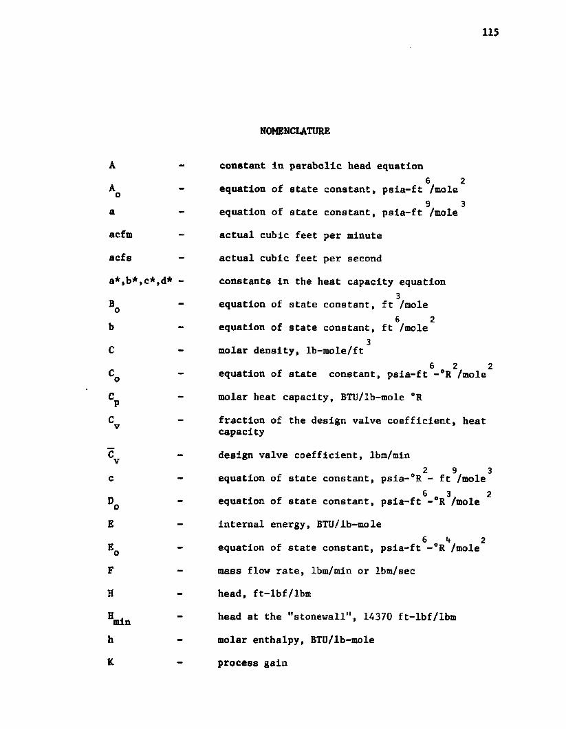
115

NOMENCLATURE

A - constant In parabolic head equation6 2Aq - equation of state constant, psia-ft /mole9 3a - equation of state constant, psia-ft /mole

acfm - actual cubic feet per minute

acfs - actual cubic feet per second

a*,b*,c*,d* - constants in the heat capacity equation3- equation of state constant, ft /mole6 2b - equation of state constant, ft /mole

3C - molar density, lb-mole/ft6 2 2CQ - equation of state constant, psia-ft -°R /mole

Cp - molar heat capacity, BTU/lb-mole °R

C - fraction of the design valve coefficient, heatcapacity

Cv - design valve coefficient, lbm/min„ 2 9 , 3c - equation of state constant, psia- R - ft /mole

6 „ 3 2Dq - equation of state constant, psia-ft - R /mole

E - internal energy, BTU/lb-mole6 i + 2Eq - equation of state constant, psia-ft -°R /mole

F - mass flow rate, lbm/min or lbm/sec

H - head, ft-lbf/lbm

®min ” head at the "stonewall", 14370 ft-lbf/lbm

h - molar enthalpy, BTU/lb-mole

K - process gain

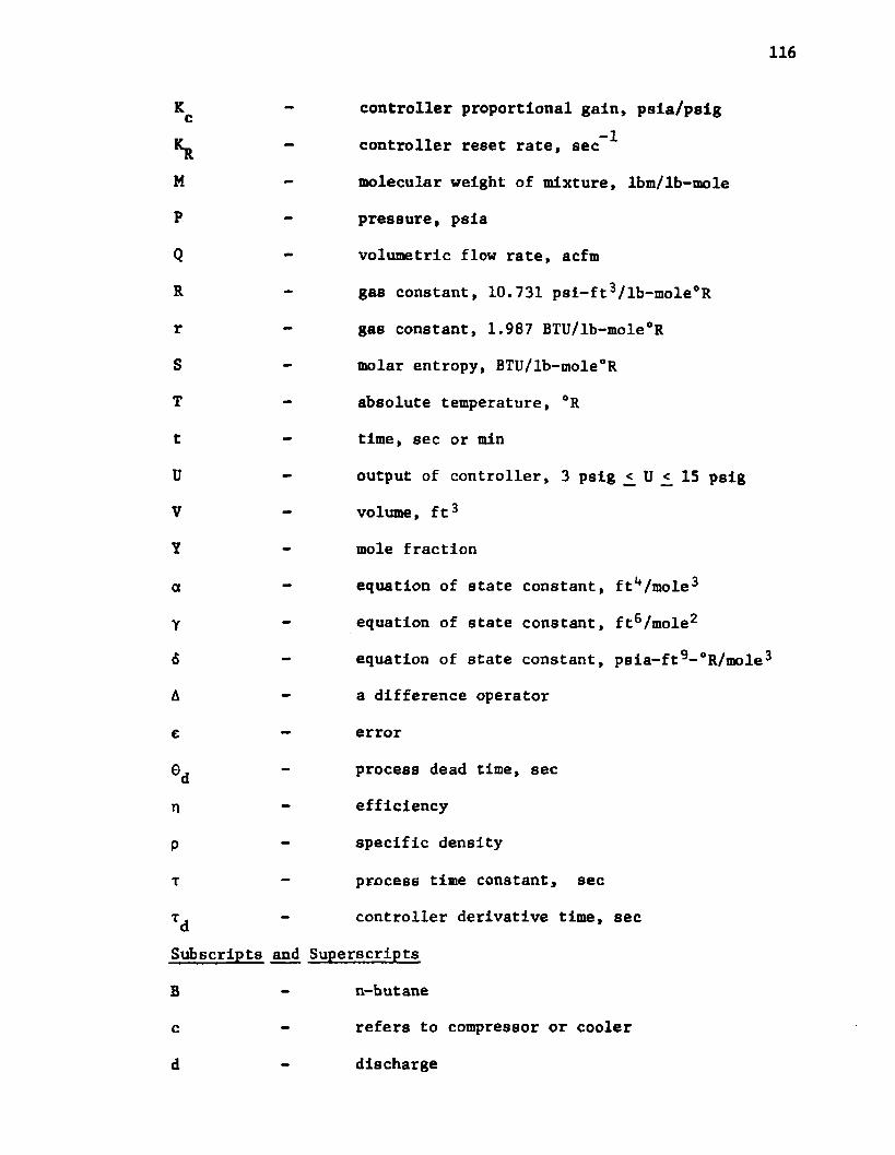
116

Kc — controller proportional gain, psia/pslg

Kr - controller reset rate, sec *

M - molecular weight of mixture, lbm/lb-moleP - pressure, psla

Q - volumetric flow rate, acfmR - gas constant, 10.731 psi-ft^/lb-mole°R

r - gas constant, 1.987 BTU/lb-mole°R

S - molar entropy, BTU/lb-mole°R

T - absolute temperature, °R

t - time, sec or min

U - output of controller, 3 psig <_ U 15 pslg

V - volume, ft3

Y - mole fraction

a - equation of state constant, ft1*/mole3

Y - equation of state constant, ft6/mole2

6 - equation of state constant, psia-ft9-°R/moJ

A - a difference operator

£ - error

Qd - process dead time, sec

n - efficiency

p - specific density

T - process time constant, sec

Td - controller derivative time, sec


B - n-butane

c - refers to compressor or cooler

d _ discharge

117

di - Isentropic discharge

E - ethane

e ~ refers to bypass loop

i - inlet, isentropic

n - mixture

o - outlet

P - propane

s - suction

ss - steady-state

v - valve

LITERATURE CITED

Starling, K. E., "Thermo Data Refined for LPG, Fart 1: Equationof State and Computer Prediction", Hydrocarbon Processing,(Mar. 1971), pp. 101-104.

Starling, K. E., "Thermo Data Refined for LPG", HydrocarbonProcessing, "Part 2: Methane?'and "Part 3: Ethane", (Apr. 1971),pp. 139-145, "Part 4: Propane" and "Part 5: n-Butane",(June 1971), pp. 116-122 and "Part 6: n-Pentane" and "Part 7:n-Hexane", (July 1971), pp. 115-121.

Benedict, M., Webb, G. B. and Rubin, L. C., Journal of Chemical Physics. 10, (1942), pp. 747-758.

CHAPTER IV

THE VARIABLE SPEED MODELS

Introduction

All centrifugal compressors are In fact variable speed machines.

They each have the capability to be operated over a range of speeds

which encompasses the stated specific speed upon which their design

is based. This range of speeds generally varies from fifty to

seventy percent of the design speed to one hundred and five to

one hundred and ten percent of the design speed depending upon

the particular application. The criterion which determines whether

they are called constant or variable speed machines is the driver.

If the driver can and is operated over a range of speeds, then the

associated compressor is classified as a variable speed machine

while if the driver is constrained to operate at a fixed speed the

associated compressor is classified as a constant speed machine.

Centrifugal compressors which are operated at a constant

speed are in most cases driven by some type of electric motor. Be

cause the motor can not in general be designed to operate at the

high speeds typical of centrifugal compressors, a speed increasing

gear is required to couple the motor to the compressor. This can

be a highly inefficient operation and as a consequence the majority

of the larger centrifugal compressors found in the process indus

tries are driven by prime movers which are characterized by speed

119

120

ranges which match the speed range of the centrifugal compressor.

Such prime movers are the steam and gas turbines.

There are, of course, other reasons for operating the compressor

as a variable speed machine and each of them stems primarily from eco

nomic considerations concerning the prime mover. If a tail gas or

other byproduct gas suitable for burning is available, the gas turbine

is the likely choice. If high pressure steam is a byproduct of the

process or is otherwise readily available then a condensing or extrac

tion steam turbine would probably be chosen. Finally, the variable

speed centrifugal compressor offers a wider range of controllable dis

charge pressure and hence greater flexibility through the controlled

variation of the speed of the prime mover. Discharge pressure control

through the manipulation of the speed of the driver also results in

savings in operating costs since there are no head losses as there

are across the throttle valve utilized in either suction or discharge

throttle control. References [1] through [8], given at the end of

this chapter, present detailed and thorough analyses of the considera

tions involved in choosing the prime mover and the Increased capabi

lities obtained when a variable speed compressor is utilized.

Because of their wide use, a study involving the simulation of

the centrifugal compressor would be incomplete without an analysis of

the variable speed machine and this chapter is devoted to this end.

The models, the CSIGM and the CSRGM, developed in Chapters II and III

respectively, require only minor modifications to be converted from

constant speed to variable speed models and as such only these modi

fications will be presented. They are presented in part through a

unique correlation of the variable speed performance map. The

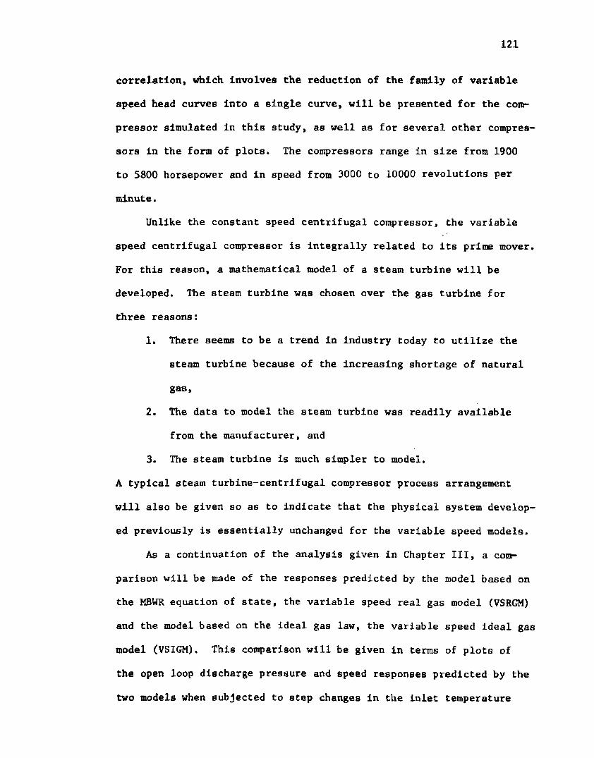
121

correlation, which Involves the reduction of the family of variable

speed head curves into a single curve, will be presented for the com

pressor simulated in this 9tudy, as well as for several other compres

sors in the form of plots. The compressors range in size from 1900

to 5800 horsepower and in speed from 3000 to 10000 revolutions per

minute.

Unlike the constant speed centrifugal compressor, the variable

speed centrifugal compressor is integrally related to its prime mover.

For this reason, a mathematical model of a steam turbine will be

developed. The steam turbine was chosen over the gas turbine for

three reasons:

1. There seems to be a trend in industry today to utilize the

steam turbine because of the increasing shortage of natural

gas,

2. The data to model the steam turbine was readily available

from the manufacturer, and

3. The steam turbine is much simpler to model.

A typical steam turbine-centrifugal compressor process arrangement

will also be given so as to indicate that the physical system develop

ed previously is essentially unchanged for the variable speed models.

As a continuation of the analysis given in Chapter III, a com

parison will be made of the responses predicted by the model based on

the MBWR equation of state, the variable speed real gas model (VSRGM)

and the model based on the ideal gas law, the variable speed ideal gas

model (VSIGM). This comparison will be given in terms of plots of

the open loop discharge pressure and speed responses predicted by the

two models when subjected to step changes in the inlet temperature

122

and pressure, the gas molecular weight, the load demand rate, and

the speed of the prime mover. A closed loop analysis will not be

given as it is felt that a major research effort in itself is required

to adequately develop such an analysis.

The Plant

The plant or physical system upon which the development of the

VSIGM and VSRGM is based is shown in Figure IV-1. It consists of a

steam turbine directly coupled to a one stage, multiwheel variable

speed centrifugal compressor. With respect to the compressor and

its suction and discharge systems, this plant is exactly the same,

physically, as the plant utilized in the development of the constant

speed models. The piping and control valves are the same size

because the compressor performance curve utilized in the constant

speed models is the design curve of this variable speed compressor.

For this reason the steady state design given in Appendix A is

valid for both the constant and variable speed systems.

In an effort to present the typical arrangement for controlling

discharge pressure, the compressor has been provided with bypass for

anti-surge control and a cascaded discharge pressure to speed control

system. Even though these control loops will not be fully developed,

they have been appended so as to clarify the existence and location

of the control valves which are a part of the VSIGM and VSRGM. The

control valve in the compressor suction is, for this plant, a part

of the upstream process and as such would be controlled by some

upstream function. It is, however, the same butterfly valve utilized

in the constant speed models.

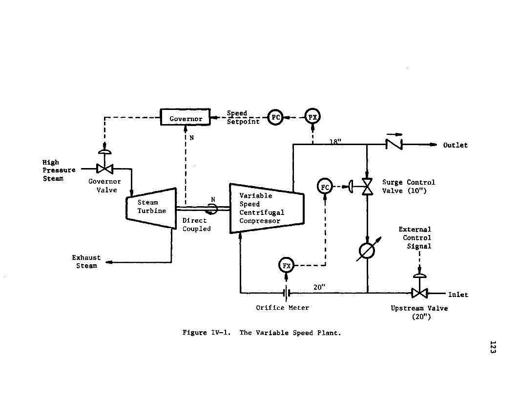
Governor

» Outlet

HighPressureSteam Governor

ValveSurge Control Valve (10")Variable

SpeedCentrifugalCompressor

SteamTurbine

DirectCoupled External

ControlSignal

ExhaustSteam

InletOrifice Meter Upstream Valve

(20")

Figure IV-1. The Variable Speed Plant.

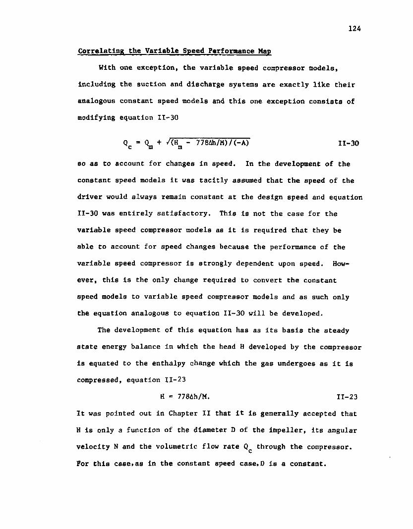
124

Correlating the Variable Speed Performance Map

With one exception, the variable speed compressor models,

Including the suction and discharge systems are exactly like their

analogous constant speed models and this one exception consists of

modifying equation 11-30

Qc - + A H n - 778Ah/M)/(-A) 11-30

so as to account for changes in speed. In the development of the

constant speed models it was tacitly assumed that the speed of the

driver would always remain constant at the design speed and equation

11-30 was entirely satisfactory. This is not the case for the

variable speed compressor models as it is required that they be

able to account for speed changes because the performance of the

variable speed compressor is strongly dependent upon speed. How

ever, this is the only change required to convert the constant

speed models to variable speed compressor models and as such only

the equation analogous to equation 11-30 will be developed.

The development of this equation has as its basis the steady

state energy balance in which the head H developed by the compressor

is equated to the enthalpy change which the gas undergoes as it is

compressed, equation 11-23

H = 778Ah/M. 11-23

It was pointed out in Chapter II that it is generally accepted that

H is only a function of the diameter D of the impeller, its angular

velocity N and the volumetric flow rate Qc through the compressor.

For this case*as in the constant speed case,D is a constant.

125

However, N is a variable and hence H Is a function of both Q andcN. This function Is developed for each compressor by the com

pressor manufacturer based upon experimental measurements on

similar machines and is expressed in the form of a compressor

performance map. This map consists of plots of H versus Qc at

various speeds for the specified design suction conditions. Figure

IV-2 gives the performance map for the compressor utilized in this

study in terms of percent of the design point. The points repre

sent data extracted from the manufacturer's map and the continuous

curves were determined from an equation which is analogous to

equation 11-24. This equation will be developed subsequently.

In order to best simulate the variable speed centrifugal com

pressor with either a digital, an analog or a hybrid computer the

relations between the three variables H, Qc> and N must be cast

into a more usable form than that given by the several curves

within the performance map. Function generators, with interpola

tion between the curves, could be used but this requires an exces

sive amount of hardware for the analog simulation and an excessive

number of calculations and possibly an excessive core requirement

for the digital simulation. In either case inaccuracies are

introduced making extrapolations in speed outside the speed range

specified by the performance map unreliable enough to be prohibitive.

One such form, which has been successfully utilized in the

simulation of variable speed centrifugal pumps and which, to this

date, has been utilized in the simulation of the centrifugal com

pressor [9-12], is the set of relations known as the Fan Law. These

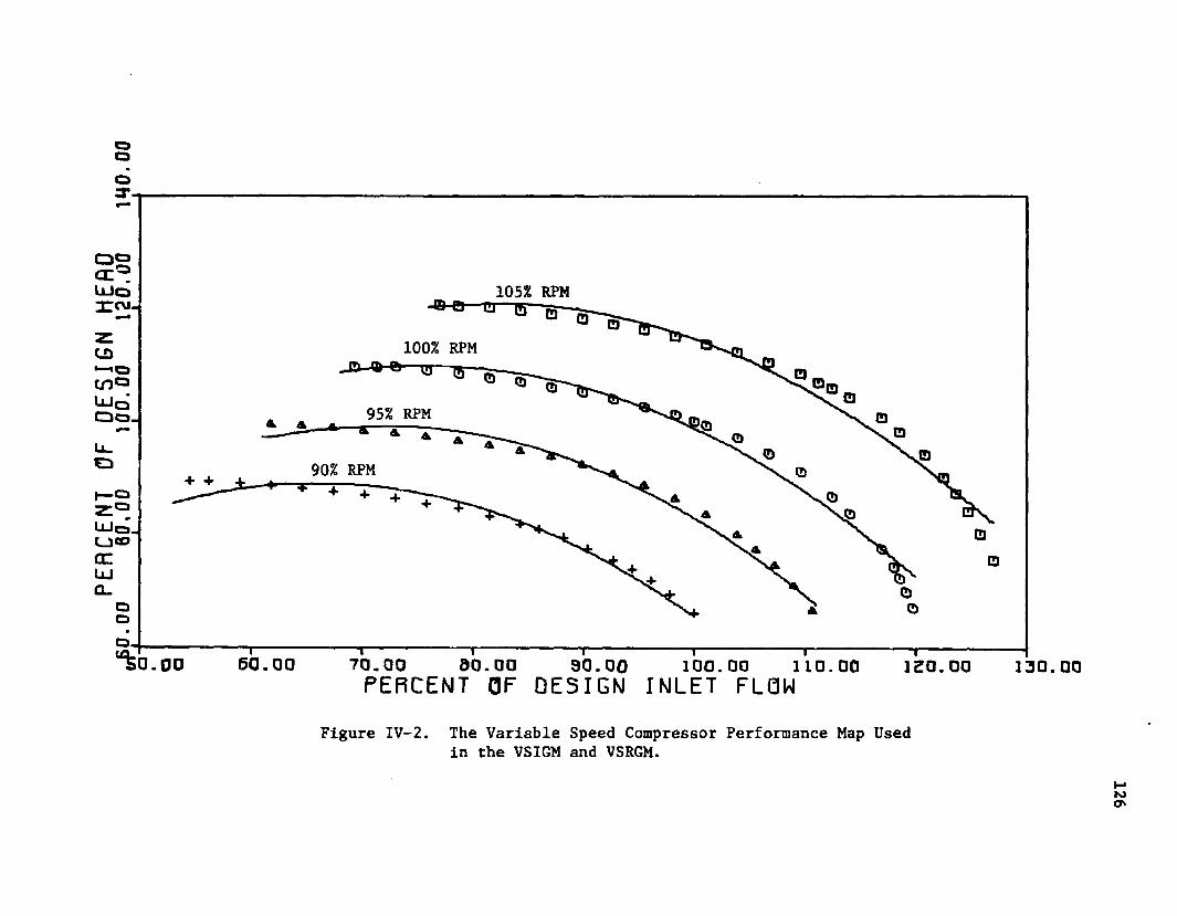
PERCEN

T OF

DESIGN

HE

RD.00

60

.00

100.

00

120.

00

140.

00

105% RPM

100% RPM

95% RPM

90% RPM

* i l l70.00 60.00 90.00 100.00PERCENT OF DESIGN INLET FLOWi------------1----------110.00 120.00 130.00“ k o . o o 6 0 . 0 0

Figure IV-2. The Variable Speed Compressor Performance Map Usedin the VSIGM and VSRGM.

126

127

relations state that power requirement Is proportional to the cube

of speed, the head Is proportional to the square of speed and the

volumetric flow rate is directly proportional to speed. The latter

two relations imply that if H/N2 is plotted versus Q/N, utilizing

points taken from the performance map, the several curves should col

lapse into a single curve. This single curve could then be utilized

in the simulation via a function generator or an equation obtained

from a statistical analysis. In general, the resulting curve is a

narrow band of points for the centrifugal pump but a widely scattered

band of points for the centrifugal compressor.

Both Shepherd [13] and Csanady [14] point out in their excellent

developments of the dimensional analysis as applied to the "pumping"

of either a compressible or an incompressible fluid that the reason

the widely scattered band of points is usually obtained for the

compressor results from the failure of the Fan Law relations to

account for compressibility effects. If the machine is a variable

speed centrifugal pump these effects are second order in nature be

cause the impeller rotates at such a slow speed and the fluid is

incompressible. This is not the case for the centrifugal compressor

as its impellers rotate at extremely high speeds,and the fluid is

compressible. Their analyses indicate that these effects must be

accounted for through the introduction of an additional term, the

Mach number. However, this parameter can only be obtained from experi

mental studies by the manufacturer or the plant personnel and as such,

efforts utilizing this concept surpass the purpose of this research.

As a result a different approach is required, one that utilizes

only the data contained within the performance map.

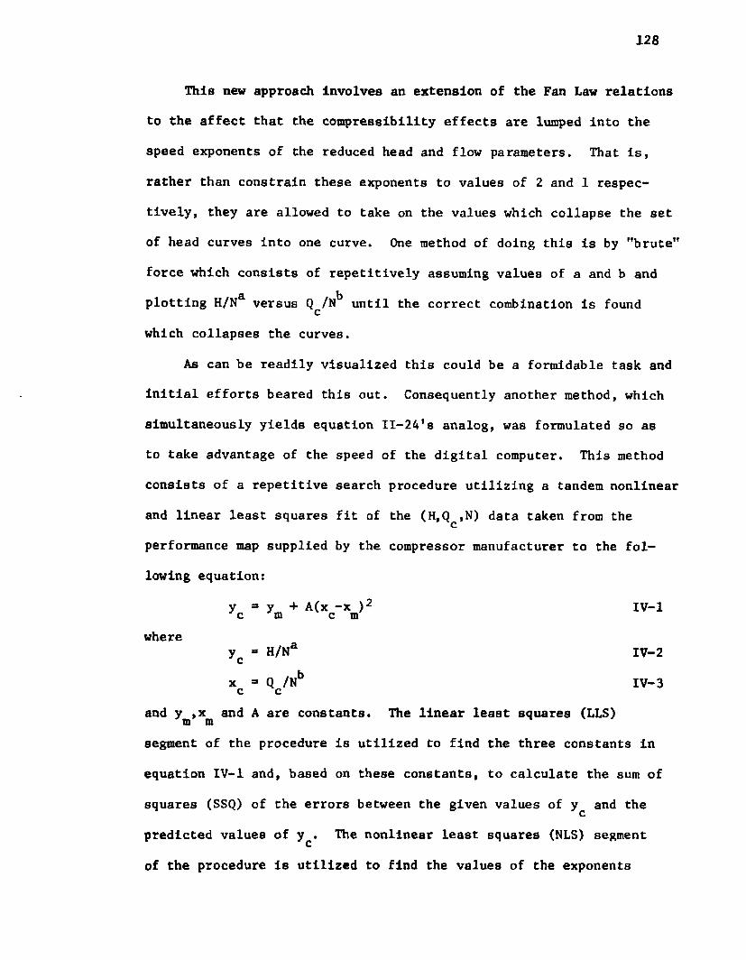
128

This new approach Involves an extension of the Fan Law relations

to the affect that the compressibility effects are lumped into the

speed exponents of the reduced head and flow parameters. That is,

rather than constrain these exponents to values of 2 and 1 respec

tively, they are allowed to take on the values which collapse the set

of head curves into one curve. One method of doing this is by "brute"

force which consists of repetitively assuming values of a and b and

plotting H/N versus Q /N until the correct combination is foundcwhich collapses the curves.

As can be readily visualized this could be a formidable task and

initial efforts beared this out. Consequently another method, which

simultaneously yields equation 11-24's analog, was formulated 90 as

to take advantage of the speed of the digital computer. This method

consists of a repetitive search procedure utilizing a tandem nonlinear

and linear least squares fit of the (H,Q ,N) data taken from thecperformance map supplied by the compressor manufacturer to the fol

lowing equation:

j - 3 ■ n VA «. j2c m c mwhere

y ■ y + A(x -x )2 IV-1c m c m

yc - H/Na IV-2

x • Q /Nb IV-3c cand y ,x and A are constants. The linear least squares (LLS) m msegment of the procedure is utilized to find the three constants in

equation IV-1 and, based on these constants, to calculate the sum of

squares (SSQ) of the errors between the given values of y and thecpredicted values of y£. The nonlinear least squares (NLS) segment

of the procedure is utilized to find the values of the exponents

129

a and b which minimizes SSQ. The technique utilized was the pattern

search developed by Moore, etal. [15] which is denoted PATERN.

A flow diagram of the procedure is given in Figure IV-3. As is

indicated an initial estimate of the values of a and b had to be

supplied. So as to insure that the final value of SSQ was not a

local minimum, sixteen different starting values were utilized.

The starting value of a was sequentially set to either 0, 1, 2, or

3 and for each, the starting value of b was set to either 0, 1, 2 or

3. For each of the performance maps correlated all sixteen starting

points produced the same final set of exponents and essentially the

same final value of the SSQ.

The result of the fit of the data indicated by the points in

Figure IV-2 is shown in Figure IV-4. The continuous curve, as well

as the continuous curves shown in Figure IV-2, were determined from

equation IV-1. Even though equation IV-1 does not exactly fit the

data it was deemed satisfactory because of its simplicity. It is

significant to note that values of a and b of 1.983 and 1.32 respec

tively, does produce collapsing of the curves into a very narrow band

of points. Scattering occurs only at the higher flow rates at which

the compressibility effects are the most significant.

In an effort to ascertain if the correlation may be considered

to be of a general nature, the (H,Qc>N) data from eight additional

performance maps obtained from various compressor manufacturers were

correlated. The data represent compressors ranging in size from

1900 to 8600 brake horsepower and in speed from 3000 to 10,000 revo

lutions per minute. Table IV-1 lists the distinguishing character

istics of each compressor and Figures IV-5 through IV-12 give plots

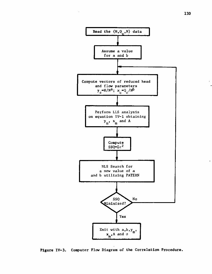
130

Read the (H,Q ,N) data

No

Yes

^ SSQ ^ Inlmized?

Assume a value for a and b

Exit with a,b,y

Perform LLS analysis on equation IV-1 obtaining

NLS Search for a new value of a

and b utilizing PATERN

Compute vectors of reduced head and flow parameters y =H/Na ; x =Q /Nb

Figure IV-3. Computer Flow Diagram of the Correlation Procedure.

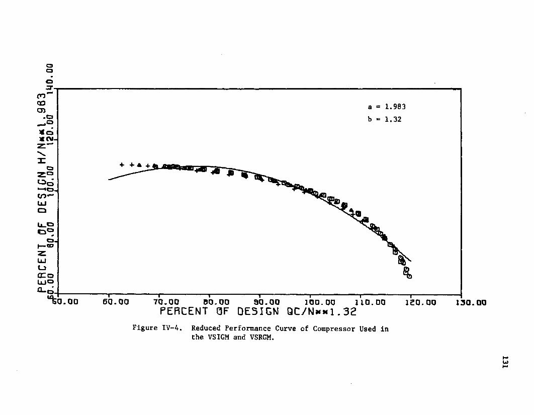
ZTcn0 305 = 1.983

1.32

O-

C_5 AC oU J Oa - D

60.00 70.00PERCENTDO.00 90.00PERCENT QF DESIGN QC/N**1.321 1 0 . 0 0100.00 130.001

Figure IV-4. Reduced Performance Curve of Compressor Used inthe VSIGM and VSRGM.

131

TABLE IV-1. COMPRESSOR CHARACTERISTICS AND CORRELATION RESULTS

BrakeHorsepower

Speed Range RPM a b 1

°1 43 4m

1900 8000-10000 2.109 1.113 1.1 1.3 1.7 952000 4000-5000 1.986 0.958 1.4 1.4 1.5 1163100 3000-5000 2.018 1.54 0.5 0.6 2.4 2083100 8000-10000 2.007 1.229 1 . 1 . 2 . 874300 8000-10000 1.879 1.128 1 1.3 1.2 985000 6000-8000 2.102 1.811 0.5 1 . 4. 2005400 4000-5000 2.019 1.27 2.2 2.2 2.8 1245800 3000-5000 2.084 1.599 0.6 1.2 5.0 16586005 4000-5000 1.983 1.32 2.4 2.4 3.0 88

^Thc standard error is calculated via: a * /le2/(M-5); e « 100(H-HP)/H; HP ■ predicted headOj is the standard error based on the given values of a and b.

202 is the standard error based on a = 2 and the given b.303 is the standard error based on a 3 2 and b ■ 1.4m is the total number of points used in the correlation.

^The bottom line of the table is for the compressor utilized in the study.

a=2.1091.113

I®%0.00 60.00 70.00 90.00 90.00 100.00 110.00PERCENT OF DESIGN QC/N**1.113 ISO.00 190.00

Figure IV-5A. Reduced Performance Curve of the 1900 Horsepower Centrifugal Compressor.

133

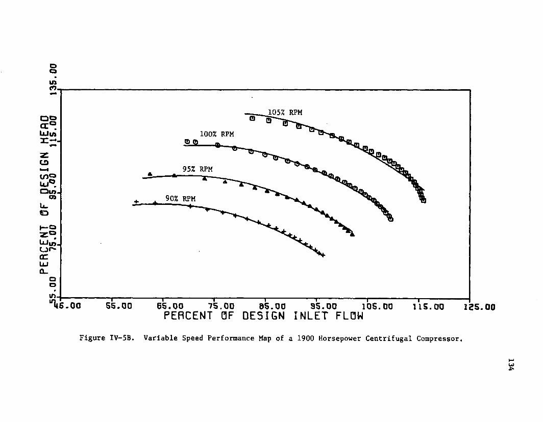
PERC

ENT

OF OES

IGN

HERO

5.00

75

.00

95.0

0 U

S.0

0 13

5.00

105% RPM

100% RPM0 e>

95% RPM

90% RPM

^ 5 . 0 0 55.00 65.00 75.00 65.00 95.00 105.00PERCENT OF DESIGN INLET FLOW U S . 0 0

Figure IV-5B. Variable Speed Performance Map of a 1900 Horsepower Centrifugal Compressor.

125.00

134

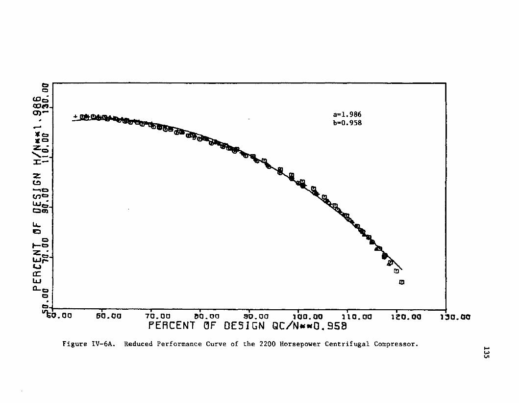
a=1.986b=0.958

UJp*'oCOUJ

70.00 00.00 90.00PERCENT 0F DESIGN QC/N««0.958M«

Figure IV-6A. Reduced Performance Curve of the 2200 Horsepower Centrifugal Compressor. 135

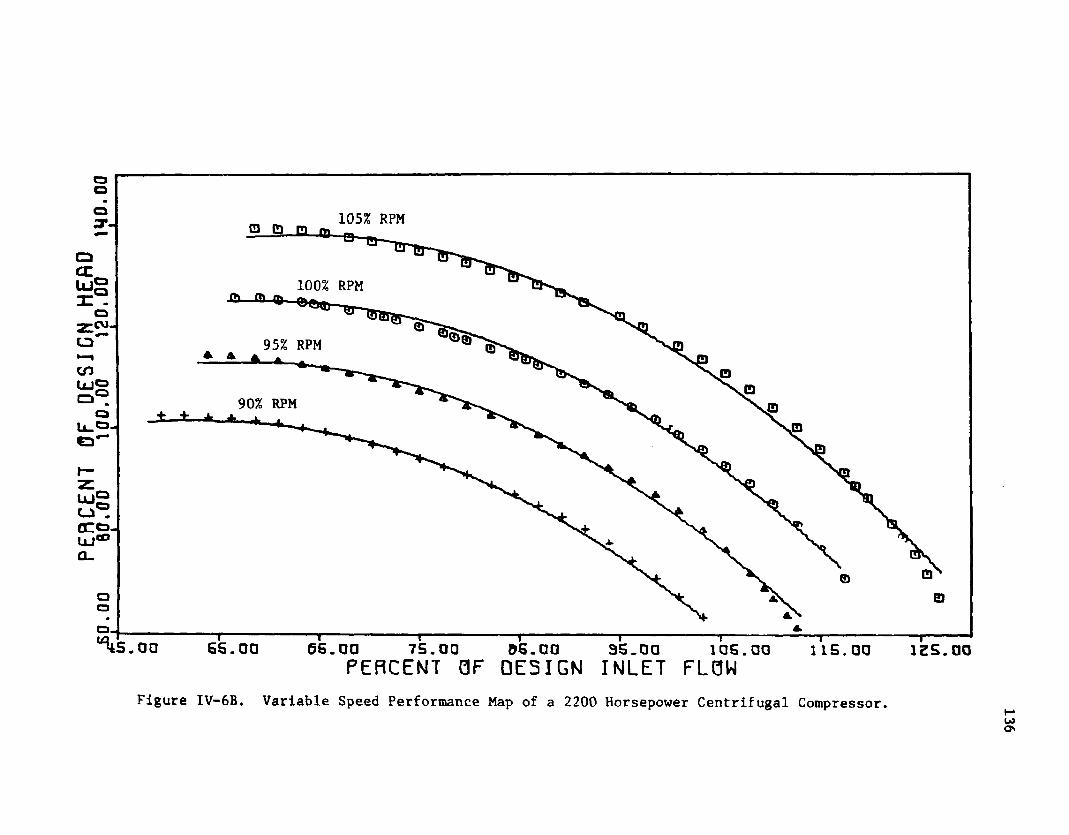
105% RPM

O(X

100% RPM ^Oqj ■ _X

95% RPMcnti lO

90% RPM

a

OS.00 35.oaPERCENT OF DESIGN INLET FLOW75.aa iis.ooPERCENTFigure IV-6B, Variable Speed Performance Map of a 2200 Horsepower Centrifugal Compressor. 136

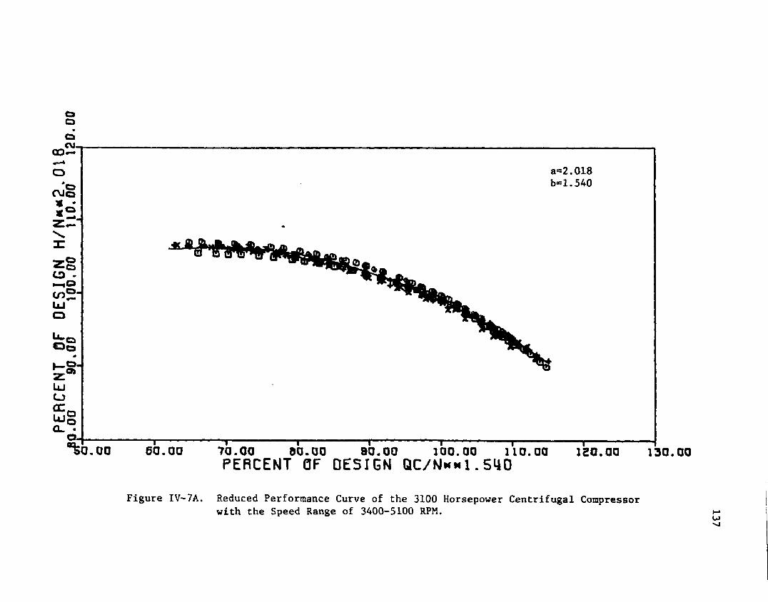
oo

00—

CVlgu ,z —

CO - «— tOcn®'

0 5O)

UJOQ C ^U g

a=2.018 b=l.540

a. “% 0 . 0 0 6 0 . QQ 7 a . 00 0 0 .0 0 8 0 . 0 0 2 0 0 .0 0 2 1 0 .0 0PERCENT OF DESIGN Q C/N«*1.540 220.00 1 3 0 . ao

Figure IV-7A. Reduced Performance Curve of the 3100 Horsepower Centrifugal Compressorwith the Speed Range of 3400-5100 RPM. »-*

-*i

oo•O

CM.105% RPM

100% RPM

95% RPM

CD90% RPM

85% RPM

80% RPM

75% RPMq 4 f70% RPM

95. QO35.00 65.00 75.00 105.00 115.00H5.00 55.00PERCENT QF DESIGN INLET FLOWFigure IV-7B. Variable Speed Performance Map of a 3100 Horsepower Centrifugal Compressor

with the Speed Range of 3400-5100 RPM.

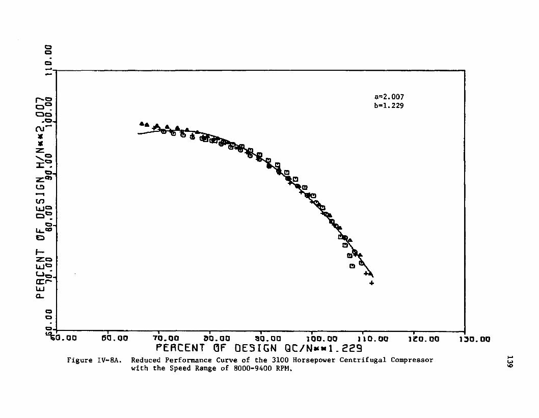
PERCEN

T OF

DESJGN

H/

N««2

.007

.00

10.0

0 60

.00

90*00

100.

00

110.

00

I I

I I

I

a=2.007 b=l.229

./■I 1 1------------------------ j I — l ~ " " "In s a . o o e a . o o t o . o q d o . o o a o . o o 1 0 0 . 0 0 i i o . o a i z o . o o i s q . o qPERCENT OF DESIGN QC/N«*.l. 229Figure IV-8A. Reduced Performance Curve of the 3100 Horsepower Centrifugal Compressor

with the Speed Range of 8000-9400 RPM.

139

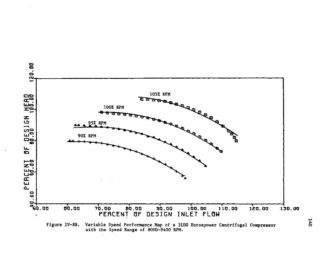
QOru.

Q OC C ®LlIo3TO-

U J ®Q o .

f— «= Z ° U J o Jt_l«©COUJ0-

aao-

105% RPM

100% RPM

95% RPM

90% RPM

GO. 0 0T T "T 1--------

00.00 70.00 DO.00 00.00 100.00 110.00PERCENT OF DESIGN INLET FLOW— 1------1Z 0 . 0 0 130.00

Figure IV-8B. Variable Speed Performance Map of a 3100 Horsepower Centrifugal Compressorwith the Speed Range of 8000-9400 RPM.

on

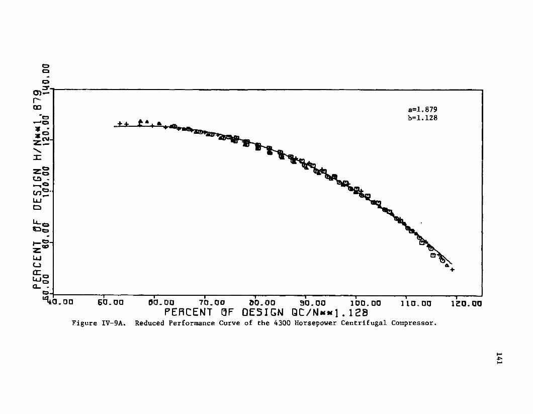
c n —r-QD a=1.879

yy CM-

e* .

LlJCD

mI— 0-11 CO

QZ.

b=l.128

LUo - _<!r □□ 60.00 — r~

0 0 .— i--------------

00 70.00 80.00 30.00 100.00PERCENT 3F DESIGN QC/N«*1.128Reduced Performance Curve of the 4300 Horsepower Centrifugal Compressor.

— r~ 30. 1 1 0 . 0 0

Figure IV-9A.

120.00

141

105% RPMCO-100% RPM

O

95% RPM

90% RPMmLUo:

SO. 00 0 0 . 0 0 70.00 1 0 0 . 0 0 1 1 0 . 0 0 ISO.00PERCENT OF DESIGN INLET FLOWFigure IV-9B. Variable Speed Performance Map of a 4300 Horsepower Centrifugal Compressor.

m

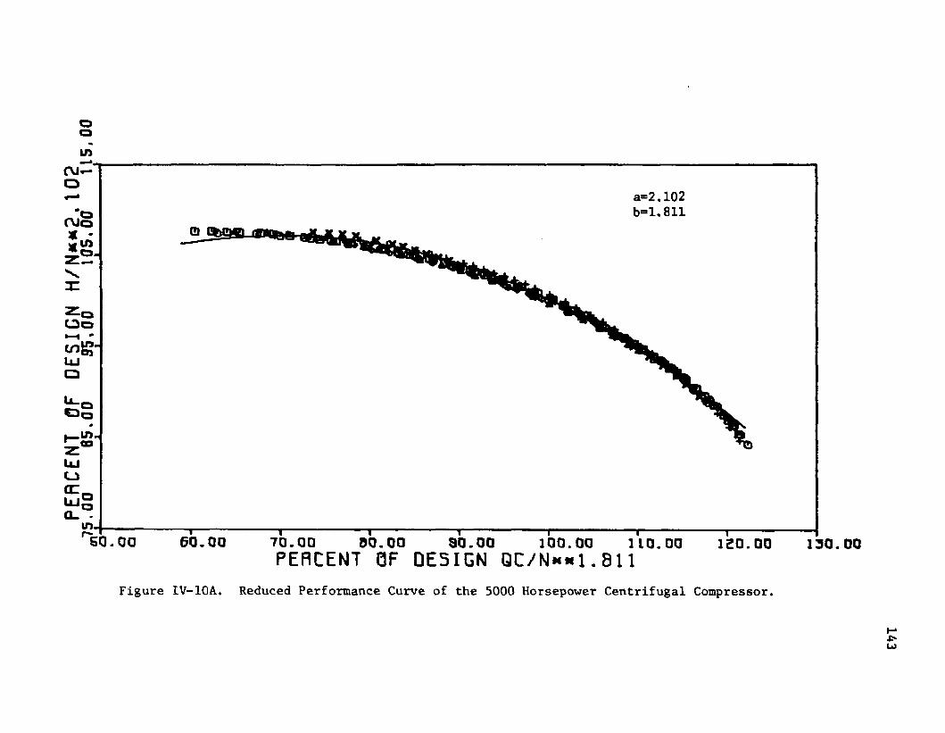
IArvj^ o

rvjo« -wini o J

C2 o

LU O

oQ 5

COa'oin.

a=2.102 b=1.811

Q %

SO-00 60.00 70.00 90.00 00.00 100.00 110.00PERCENT OF DESIGN QC/N«*1.811 ISO.00 130.00

Figure IV-10A. Reduced Performance Curve of the 5000 Horsepower Centrifugal Compressor.

143

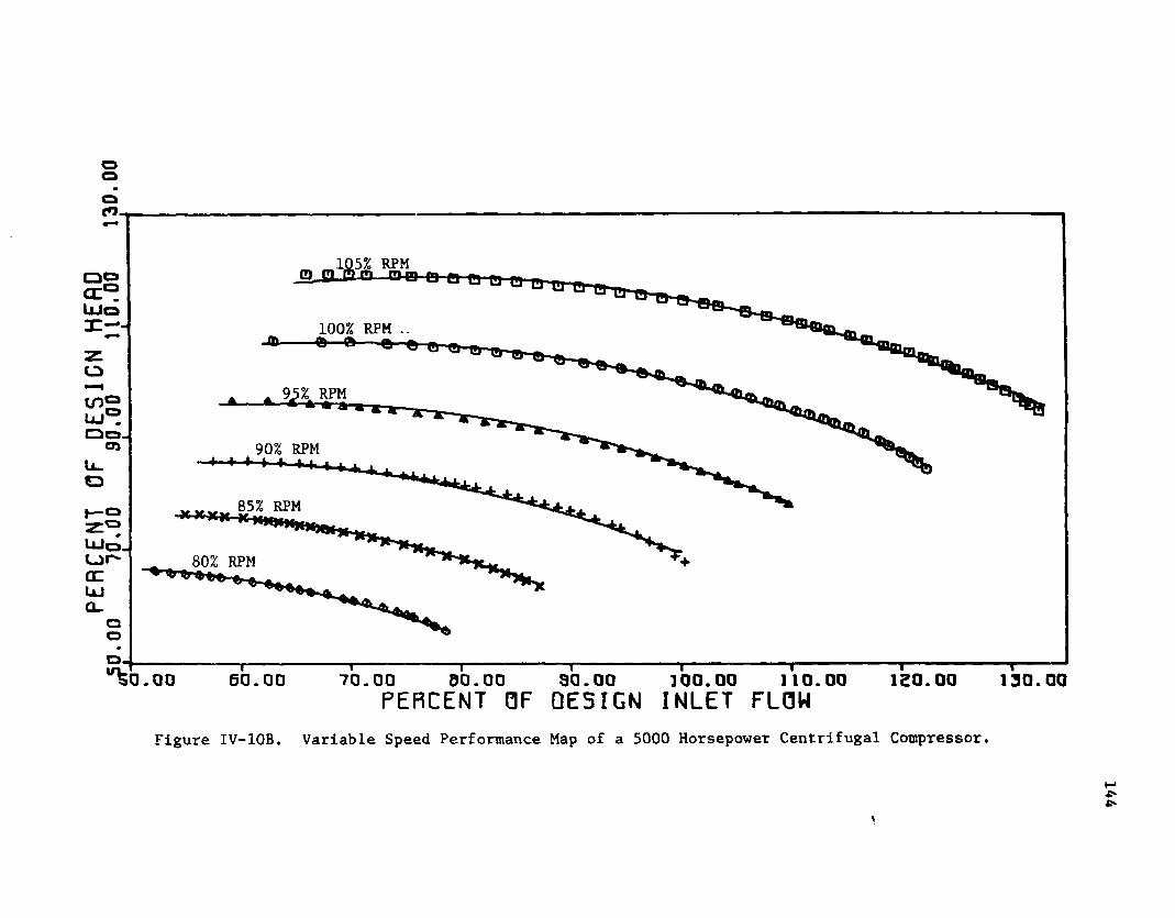
o

<n

RPM

90% RPM

85% RPM

Li-lt—«Ljr-CCLUQ_

a

80% RPM

60. 00 190.0000.00 90.00 100.0070.00PERCENT OF QE5IGN INLET FLOWFigure IV-10B. Variable Speed Performance Map of a 5000 Horsepower Centrifugal Compressor.

\

m

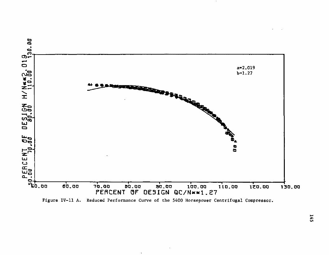
o a=2.019b=1.27

X

cr>S5UJo

t_5COUJQ-

70.00 DO.00 30.00 100.00PERCENT 0F DESIGN QC/N«*1.27 1 1 0 .oo 1 2 0 .oo 130.00

Figure IV-11 A. Reduced Performance Curve of the 5400 Horsepower Centrifugal Compressor.

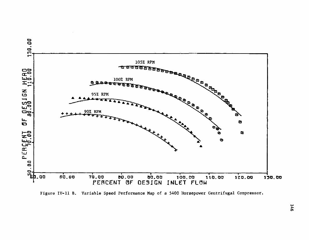
PERCEN

T OF

DESIGN

HE

RO"S

O.00

10.00

90.00

110.

DO 13

0.00

tfr I__

_________I

I I

1

105% RPM

100% RPMJs j b m « gj m ft

95% RPM 5 - ^ * * * T 4 4 -y

90% RPM4■ 4■

1 1 1 1 1 1 1----------3.00 60.00 70.00 90.00 90.00 100.00 110.00 120.00 130.00PERCENT 0F DESIGN INLET FLOW

Figure IV-11 B. Variable Speed Performance Map of a 5400 Horsepower Centrifugal Compressor,

146

§2.084

b-1.599

65.00 75.00 05.00 85.00 105.00 115.00PERCENT OF DESIGN D C/N««1.599 125.00 135.00

Figure IV-12 A. Reduced Performance Curve of the 5800 Horsepower Centrifugal Compressor.

147

105% RPM

100% RPMCD

95% RPM

90% RPMIS)£CD 85% RPM

80% RPM

75% RPM

70% RPM

70.00 00.0Q 90.00 120.00PERCENT OF DESIGN INLET FLOWFigure IV-12 B. Variable Speed Performance Map of a 5800 Horsepower Centrifugal Compressor.

149

of the resulting fits In terns of the reduced parameters and In terns

of H, Qc and N. The constants and the design point data will not be

given as this information has been restricted by the compressor

manufacturers.

Also included in Table IV-1 are three different values for the

standard error of the fit. 0 } is based on the values of a and b given

in the table, a2 is based on the value of two for a and the given

value for b while 03 is based on the values of two for a and one for

b. Each of the fits yielded essentially the same values of x , ytn mand A and hence the three values of the standard error of the fit

provide a qualitative comparison of the effectiveness possessed by

each set of exponents to bring about collapsing of the head curves.

A comparison of and o2 indicates that the exponent a could

have been given the value two for each of the compressors except

the 1900, 5000 and 5800 horsepower ones. A further comparison of

Oj and o 3 indicates that only the 2000 and the 4300 horsepower

machines possess curves which can be correlated with an a of two and

a b of one. The major difference between these two machines and the

others is that they were designed with a pressure ratio of two while

the others were designed with pressure ratios ranging from three to

seven. This explains the fit since at the lower pressure ratios the

compressibility effects are second order. With the exception of

these two machines, an a of two and a b of one produces an unaccept

able scattering of the resulting reduced performance curve as is

evidenced by the larger values of 0 3.

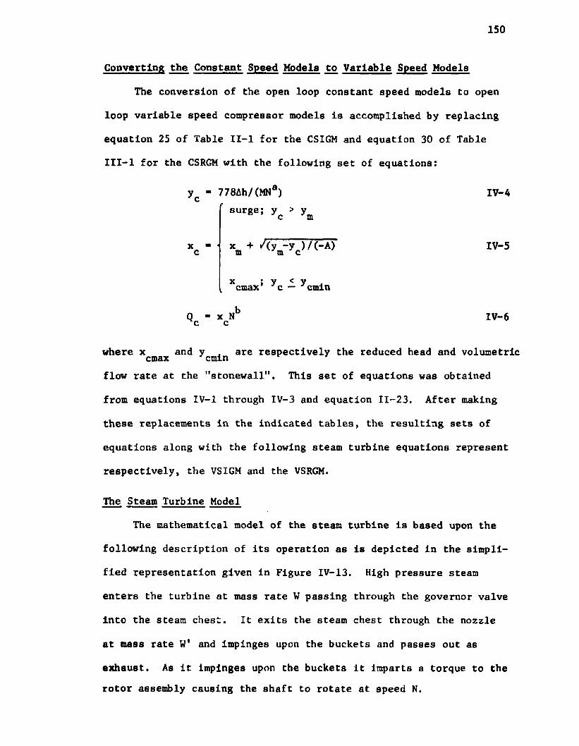
150

Converting the Constant Speed Models to Variable Speed Models

The conversion of the open loop constant speed models to open

loop variable speed compressor models Is accomplished by replacing

equation 25 of Table II-l for the CSIGM and equation 30 of Table

III-l for the CSRGM with the following set of equations:

flow rate at the "stonewall". This set of equations was obtained

from equations IV-1 through IV-3 and equation 11-23. After making

these replacements In the Indicated tables, the resulting sets of

equations along with the following steam turbine equations represent

respectively, the VSIGM and the VSRGM.

The Steam Turbine Model

The mathematical model of the steam turbine is based upon the

following description of its operation as is depicted in the simpli

fied representation given in Figure IV-13. High pressure steam

enters the turbine at mass rate W passing through the governor valve

Into the steam chest. It exits the steam chest through the nozzle

at mass rate W' and impinges upon the buckets and passes out as

exhaust. As it impinges upon the buckets it Imparts a torque to the rotor assembly causing the shaft to rotate at speed N.

y - 778Ah/(MNa)f surge; y > y c m

IV-4

IV-5

cmin

Q ■ x Nc c.b IV- 6

where xcmax and ycmLn are respectively the reduced head and volumetric

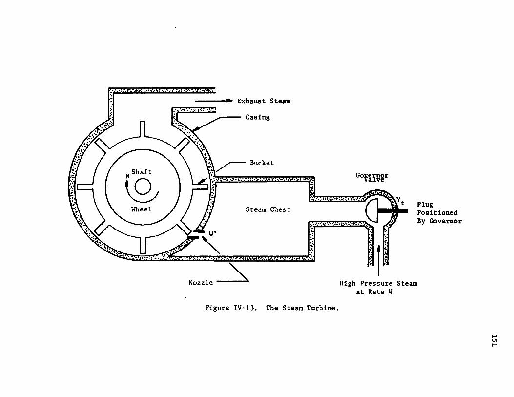
rj*TvT?T 1*»

Shaft

Wheel

Exhaust Steam

Casing

Bucket

• V.v* :i;-v. .».v*r ■•w.v.-ii »i%m ' Go iiv81

Steam Chest

;V

PlugPositioned By Governor

Nozzle High Pressure Steam at Rate W

Figure IV-13. The Steam Turbine.

151

152

The equation required to represent this operation results from

a torque or momentum balance taken about the turbine rotor. This

balance equates the rate of accumulation of momentum to the dif

ference between the torque T produced by the high pressure steam as

where I Is the moment of Inertia of the rotor assembly and which Is

supplied by the manufacturer. The load torque is equal to the

power demand of the compressor divided by the speed of the shaft

and the efficiency of the turbine which is also supplied by the manu

facturer

The torque produced by the high pressure steam as it passes

through the turbine is determined from a map of the turbine's per

formance characteristics which is developed by the turbine manufac

turer based on experimental measurements of similar machines. A

typical performance map gives the steam mass rate through the

throttle valve as a function of the developed horsepower with speed

as a parameter. The performance map of the turbine upon which the

model is based is shown in Figure IV-14 in which percent of design

steam rate is plotted versus percent of design horsepower. This

map was received from the General Electric Company [16] and it

represents the performance of a steam turbine which is in operation

today.

It passes through the turbine and the load torque T which isLdemanded by the compressor

IV-7

F H c IV- 82IINn c

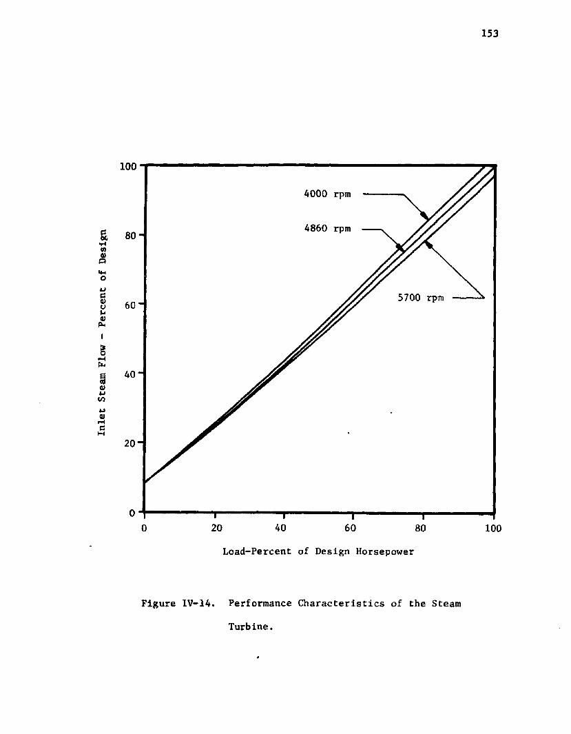
Inlet

Steam

Flow

- Percent

of De

sign

153

100

4000 rpm

4860 rpm

5700 rpm

40

20 -

4020 600 80 100Load-Percent of Design Horsepower

Figure IV-14. Performance Characteristics of the Steam

Turbine.

154

Since Che three curves are so close together, It was assumed

that the middle curve would adequately represent the performance of

the turbine. Also, since the curve is essentially linear, it was

assumed that a straight line equation would suffice and the slope

and intercept were determined from the manufacturer’s map resulting

inW - aL + b IV-9

where L is load in horsepower. Multiplication of the slope by the

factor 2IIN/33000 converts it from horsepower to torque resulting

in

T “ ! n r ( w - b ) IV-10

which is the desired equation which relates the torque developed by

the steam as it passes through the turbine to the rate of flow of

the steam into the turbine. Thus, the equation required to describe

the dynamics of the turbine's rotor is

N - m i v - u

where TL and T are given respectively by equation IV-8 and IV-10.

To maintain the speed of the turbine at a desired value, a

governor assembly, which is a complex hydromechanical mechanism is

provided. It senses N through a gear assembly and produces a power

piston movement of Z inches if there is an error between the desiredgspeed and N. This movement causes, through a mechanical linkage,

the governor valve plug to move Y inches which changes the inlet

rate of steam and thus the speed of the shaft.

Even though the governor will not be included in the model the

equations representing the dynamics of the valve and its positioner

155

as well as the valve flow characteristics have been Included so that

the open loop response of the compressor and turbine could be deter

mined for changes In the governor output. The flow characteristics

of the valve are based on data received from General Electric [16]

and are shown in Figure IV-15. This function was implemented into

the model via a function generator.

The equation required to describe the dynamics of the valve and

Its positioner is also based on information received from General

Electric [16], and is obtained from the following considerations.

First, assume that as the power piston moves from 0 to 1.25 inches,

the normalized throttle valve position varies from 0 to 1. Further

assume that the valve dynamics can be adequately described by a first

order lag with a time constant of 2.6 seconds. Then the required

equation is

Y - ^ r (°.8 Z -Tf ). IV-11t 2.0 g t

The final equation required to model the steam turbine stems

from a mass balance about the steam chest. A Control Systems Analyst

of General Electric [17] has indicated that a first order lag with

a time constant of 0.1 seconds adequately describes the process as

determined from experimental measurements. Thus for a steam rate

into the stem chest of W and a steam rate out of W', the equation

becomes

W* - 10 (Vf-W). IV-12

An Information flow diagram summarizing these developments is

given In Figure IV-15. It also indicates the coupling between the

variable speed compressor and the steam turbine.

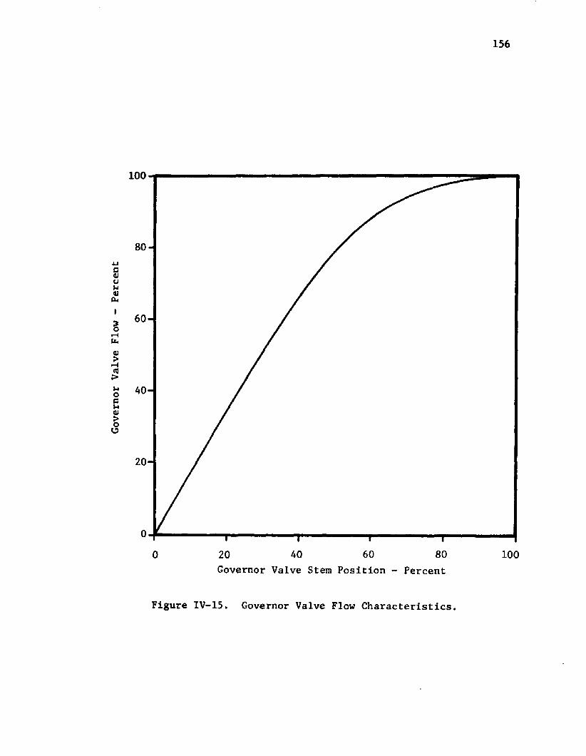
Governor Valve

Flow

- Pe

rcen

t

156

100

80

60

40

20

0

0 20 40 60 80 100Governor Valve Stem Position - Percent

Figure IV-15. Governor Valve Flow Characteristics.

Load.Torque Rotor Dynamics

Load Variables

Steam Turbine Performance CharacteristicsSteam Chest Lag

T=K W'-B

VariableSpeed

CompressorModel

Governor Valve Flow Characteristics

W

Governor Valve and Positioner Dynamics

Governor

Figure IV-16. The Steam Turbine Model.

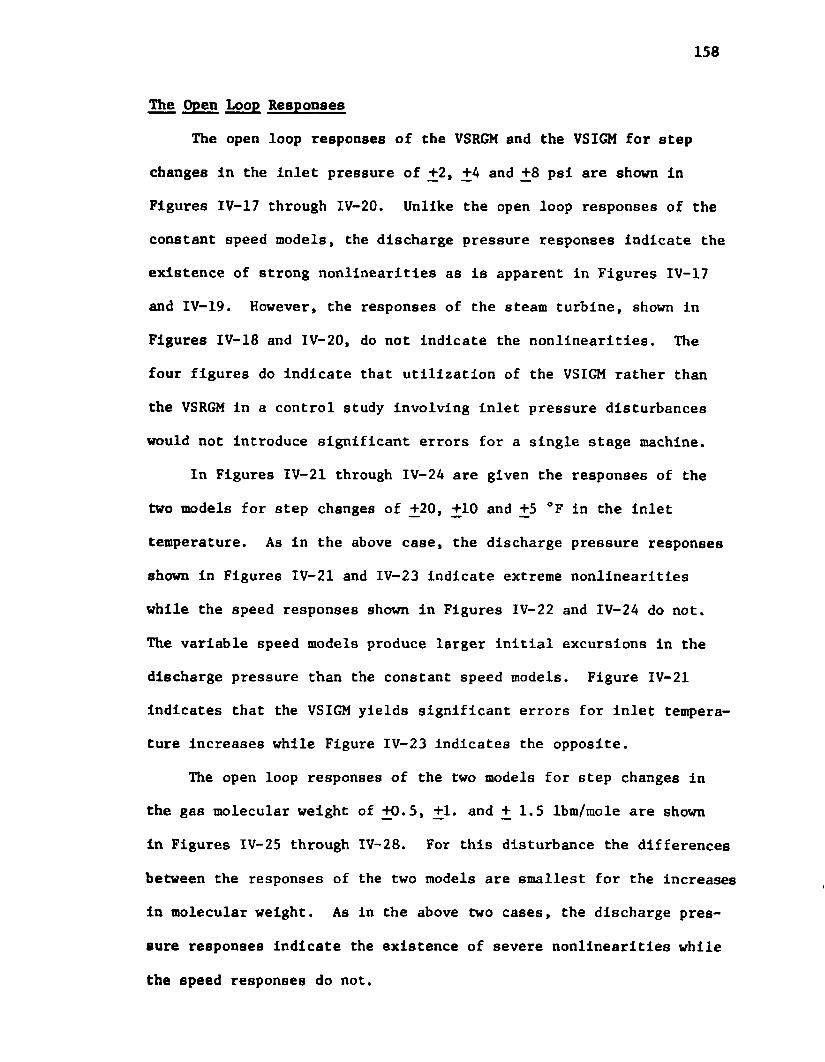
158

The Open Loop Responses

The open loop responses of Che VSRGM and the VSIGM for step

changes In the Inlet pressure of +2, +4 and +8 psl are shown in

Figures IV-17 through IV-20. Unlike the open loop responses of the

constant speed models, the discharge pressure responses indicate the

existence of strong nonlinearities as is apparent in Figures IV-17

and IV-19. However, the responses of the steam turbine, shown in

Figures IV-18 and IV-20, do not indicate the nonlinearities. The

four figures do Indicate that utilization of the VSIGM rather than

the VSRGM in a control study involving inlet pressure disturbances

would not introduce significant errors for a single stage machine.

In Figures IV-21 through IV-24 are given the responses of the

two models for step changes of +20, +10 and +5 °F in the inlet

temperature. As in the above case, the discharge pressure responses

shown in Figures IV-21 and IV-23 indicate extreme nonlinearities

while the speed responses shown in Figures IV-22 and IV-24 do not.

The variable speed models produce larger initial excursions in the

discharge pressure than the constant speed models. Figure IV-21

Indicates that the VSIGM yields significant errors for inlet tempera

ture increases while Figure IV-23 indicates the opposite.

The open loop responses of the two models for step changes in

the gas molecular weight of +0.5, +1. and +1.5 lbm/mole are shown

in Figures IV-25 through IV-28. For this disturbance the differences

between the responses of the two models are smallest for the increases

in molecular weight. As in the above two cases, the discharge pres

sure responses Indicate the existence of severe nonlinearities while

the speed responses do not.

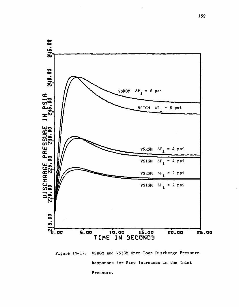
159

VSRGM AP1 = 8 psi

VSIGM APi = 8 psi

VSRGM AP

4 psiVSIGM AP

2 psiVSRGM AP

VSIGM AP

‘' b . o o 6.OQ IQ.00 15.00TIME IN 3ECGND5 ZO. 00 Z 5 .00

Figure IV-17. VSRGM and VSIGM Open-Loop Discharge Pressure

Responses for Step Increases in the Inlet

Pressure.

SPEEO

IN RP

S,16

.00

11.0

0 16

.00

10.0

0 60

.00

61.0

0 82

.00

I •

a a

a I

l l

160

4P, = 2 psiVSRGM

VSIGM

" ------- --------- = 4 psi

VSIGM

VSRGM

VSIGM

VSRGM

Q. 00 6 . 0 0 1 0 . 0 0 1 5 . 0 0 2 0 . 0 0t i m e i n s e c o n d s

Figure IV-18. VSRGM and VSIGM Open-Loop Speed Responses for

Step Increases In the Inlet Pressure.

25.00

161

ooincuCM

CM,CM

<XVSIGM

VSRGM

VSIGM

VSRGM

VSIGM

VSRGM

CM

0 . 0 0 6.00 15.001 0 . 0 0 25.00TIME IN SECONDSFigure IV-19. VSRGM and VSIGM Open-Loop Discharge Pressure

Responses for Step Decreases in the Inlet

Pressure.

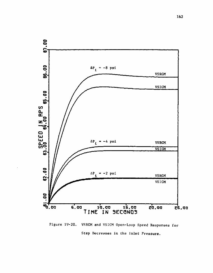
162

#

©VSRGM<000

VSIGMO

119CD

00

-4 psi VSRGMVSIGM

VSRGMVSIGM

O

IS.006. 00 10. 00 es.oot i m e i n s e c o n d sFigure IV-20. VSRGM and VSIGM Open-Loop Speed Responses for

Step Decreases in the Inlet Pressure.

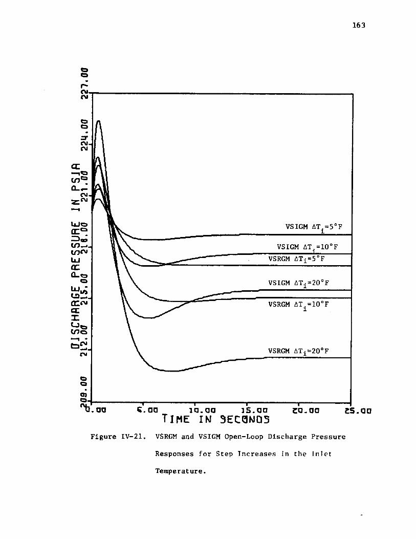
GJ SCH

RRGE

PRES

SURE

IN

PSJR

JOS.00

217.00

21

5.00

21

6.00

22

1.00

22

4.00

22

2.00

*—■ j

i .

..

.

.

163

G. 0 0

VSIGM AT^=5°F

VSIGM AT^=10°FVSRGM ATi=5°F

VSIGM ATi=20°F

VSRGM ATi=10°F

VSRGM ATi=20°F

-------- 1 i |---la.aa is.aa eo.ao es.aaT i m e i n s e c o n d s


Responses for Step Increases in the Inlet

Temperature.

164

U)r>

to

VSRGM

VSIGMtn

co

VSRGM

VSIGM

VSRGM

VSIGM

1S.Q0Q. QQ T i m e i n s e c o n d sFigure 1V-22. VSRGM nnd VSIGM Open-Loop Speed Responses

lor Step Inereases in the Inlet Tempera Lure.

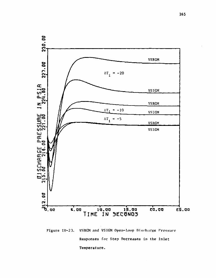
165

CM

VSRGM

-20<Mru

a :VSIGM

VSRGMAT VSIGMU J QAT -5

VSRGMVSIGM

ru

15.00C. OQ 10.QO00 T i m e i n s e c o n d s

Figure IV-23. VSRGM and VSIGM Open-Loop Discharge I’ressurc

Responses for Step Decreases in the Inlet

Temperature.

166

in4to

VSIGMino- VSRGM

VSIGM07

AT

VSRGMto

UJ VSIGM

-20°FAT

VSRGM

0 . QQt i m e i n s e c o n d s

Figure IV-24. VSRGM and VSIGM Open-Loop Speed Responses

for Step Decreases in the Inlet Temperature.

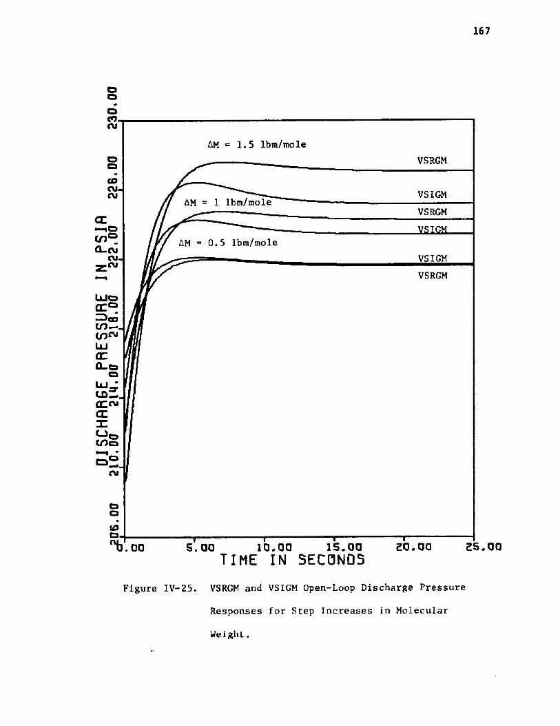
167

Oo

COCM

AM - 1.5 lbm/moleVSRGM

CDCM-CM VSIGMAM = 1 lbm/mole

VSRGM

AM = 0.5 lbm/moleQ-cmc m-t^ cm VSIGM

VSRGM

CM

DIDO

15.005.0000 TIME IN SECONDSFigure IV-25. VSRGM and VSIGM Open-Loop Discharge Pressure

Responses for Step Increases in Molecular

Wei glit.

168

OOD

VSIGMinAM = 0.5 lbm/moleo .CO VSRGM

VSIGMo AM = 1 lbm/mole

VSRGMCO

VSIGMAM = 1.5 lbm/mole

VSRGMUJIxJt n ®

o>

in

oto

1 5 . 0 0 2 5 . 0 0I d . <300.00 TIME IN SECONDSFigure IV-26. VSRGM and VSIGM Open-Loop Speed Responses

for Step Increases in Molecular Weight.

DISC

HARG

E PR

ESSU

RE

IN PS

IA10

.00

2114

.00

216.

00

222.

00

226.

00

230.

00

234.

00

169

VSIGM AM * -1 lbm/mole

VSIGM AM - -0.5 lbm/mole

VSRGM AM = -0.5 lbm/mole

VSIGM AM = -1.5 lbm/mole - VSRGM AM = -1 lbm/mole

VSRGM AM = -1.5 lbm/mole

is. 0 0OO 1 0 . 0 0TIME IN SECONDSFigure IV-27. VSRGM and VSIGM Open-Loop Discharge Pressure

Responses for Step Decreases in Molecular

We i gh t.

170

in

«o.CD

in AM = -1.5 lbm/mole VSRGMCMCDi nQ_c o

VSIGM

AM = -1 lbm/mole•— •CM.COollJ

VSRGMVSIGM

AM = -0.5 lbm/moleCO VSRGMVSIGM

CD

ain

S. 00□ 0 10.00 15.00t i m e in s e c o n d s

Figure IV—28. VSRGM and VSIGM Open-Loop Speed Responses

for Step Decreases in Molecular Weight.

171

Figures IV-29 through IV-32 give the responses of the VSRGM and

the VSIGM for step changes In the load demand rate of +5, +10 and

+15 percent of the design mass flow rate. For both the positive and

the negative step changes, there is little difference between the

predictions of the two models. The responses for the negative dis

turbances, shown in Figures IV-31 and IV-32 do not indicate any

severe nonlinearities in terms of the discharge pressure or the speed

while Figures IV-29 and IV-30 indicate extreme nonlinearities for

the positive disturbances. These four figures vividly illustrate

that the characteristics of the machines, the compressor and the

turbine, are completely different for operation above the design

point and operation below the design point.

The open loop responses of the two models for step changes in

the governor output of +0.05, +0.1 and +0.15 inches are shown in

Figures IV-33 through IV-36. In this case the responses for the

Increased governor output, shown in Figures IV-33 and IV-34 indicate

a linear process while the responses for the decreased governor out

put, shown in Figures IV-35 and IV-36 indicate a very nonlinear

process. The more linear responses indicate the greatest amount of

difference between the predictions of the two models.

The major point to be gained from an analysis of these open

loop response curves is that the variable speed tandem is much more

nonlinear than the constant speed machine. In all cases, the greatest

difference between the predictions of the two models occurs for

changes which drive the compressor beyond its normal operating point.

The responses for inlet pressure decreases, inlet temperature

Increases, molecular weight decreases, load demand rate increases,

172

ID.Ol

IDCO.CM

AF =0.05 Fdesign VSIGMdesign VSRGM

VSIGMGCQ - o VSRGM

AF =0.15 FdeSlgn VSIGMVSRGM

O

0. DO 15.005.00 20.0010.00TIME IN SECONDSFigure IV-29. 4^SRGM and VSTGM Open-Loop Discharge Pressure

Responses for Step Increases in the Load

Demand Rate.

173

oIDCD

rr.QD

.design

VSRGMVSIGMCO.

CPcn a. oc designAF

VSRGMZ 'M W .CPObJUJcl.®t o ®

VSIGM

.designVSIGM

VSRGMCD

CD

r o . o o 5.00 10.00 15.00TIME IN S ECONDSFigure IV-30. VSRGM and VSIGM Open-Loop Speed Responses for

Step Increases in the Load Demand Rate.

174

VSRGM

VSIGM

design VSRGMVSIGM

AF = -0.05 F Sign o o VSIGM

VSRGM

*'b. oo— i------------ 1 i-----5.00 10.00 15.00TIME IN SECONDS 20.00 25.00


Responses for Step Decreases in the Load

Demand Rate.

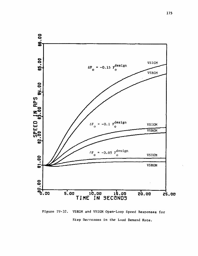
SPEEO

INRP

S

175

VSIGMAF = -0.15 F o o

VSRGM

0.1 F VSIGMVSRGM

0.05 Fdeslgn VSIGM

VSRGM

CO_

“ b . o o 1 1------------ 1— —5.00 10.00 15.00 20.00TIME IN SECCINDS 25.00

Figure IV-32. VSRGM and VSIGM Open-Loop Speed Responses for

Step Decreases in the Load Demand Rate.

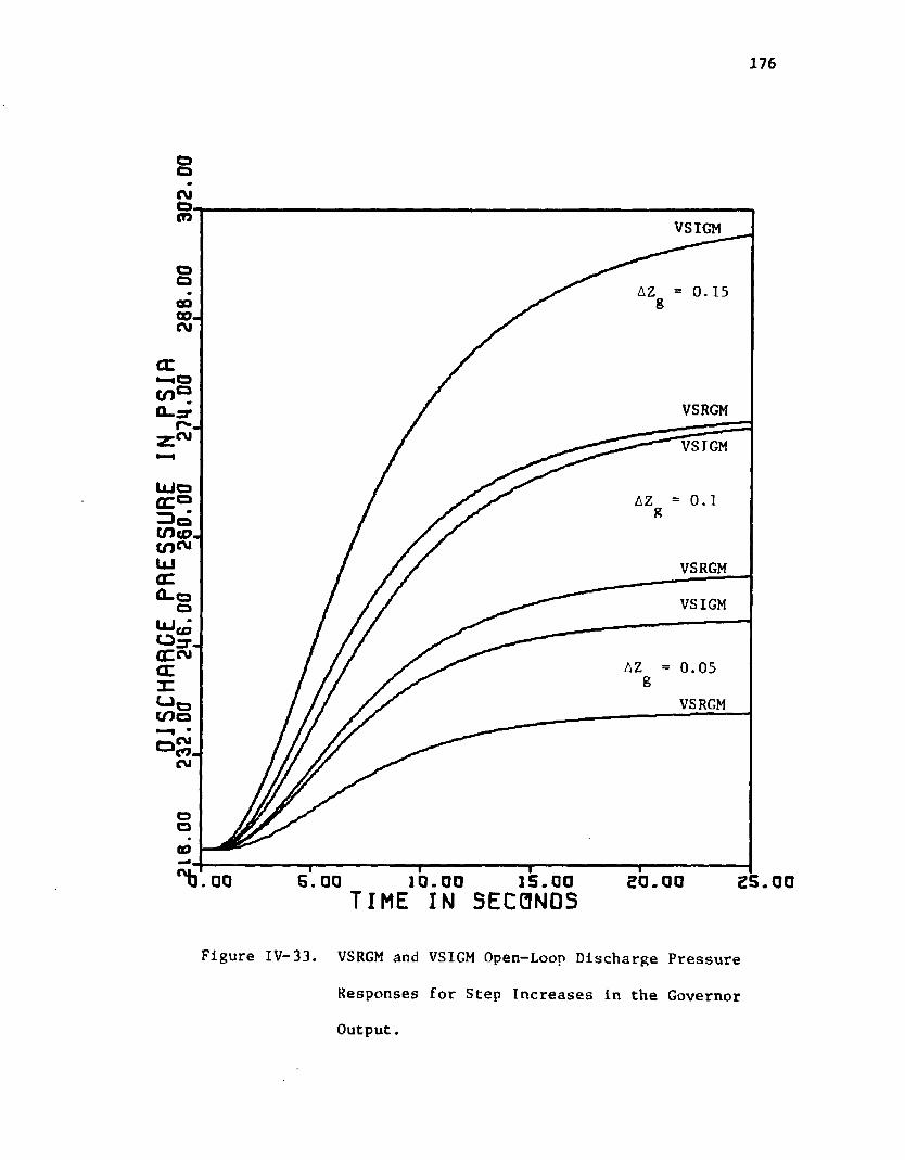
DISC

HARG

E PR

ESSU

RE

IN PS

IR16

.00

232.

00

246.

00

260.

00

274.

DO 28

B.00

30

2.00

L

L I

I I

I I

176

VSIGM

AZ 0. 15

VSRGM

VSIGM

AZ

VSRGM

VSIGM

VSRGM

5. 0 0 15.001 0 .0 0TIME IN SECONDSFigure IV—33. VSRGM and VSIGM Open—Loon Discharge Pressure

Responses for Step Increases in the Governor Output.

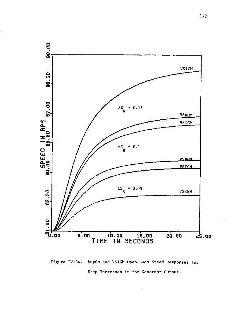
177

Oai

VSIGMLf5

0.15VSRGMflO

cnfl-OC

VSIGM

m•—•us.CDCD

YSBGEL

GO

VSRGMLT>CM-CD

O

S. 000 0 I S . 001 0 .0 0t i m e i n s e c o n d s

Figure IV-34. VSRGM and VSIGM Open-Loon Speed Responses for

Step Increases in the Governor Output.

.00

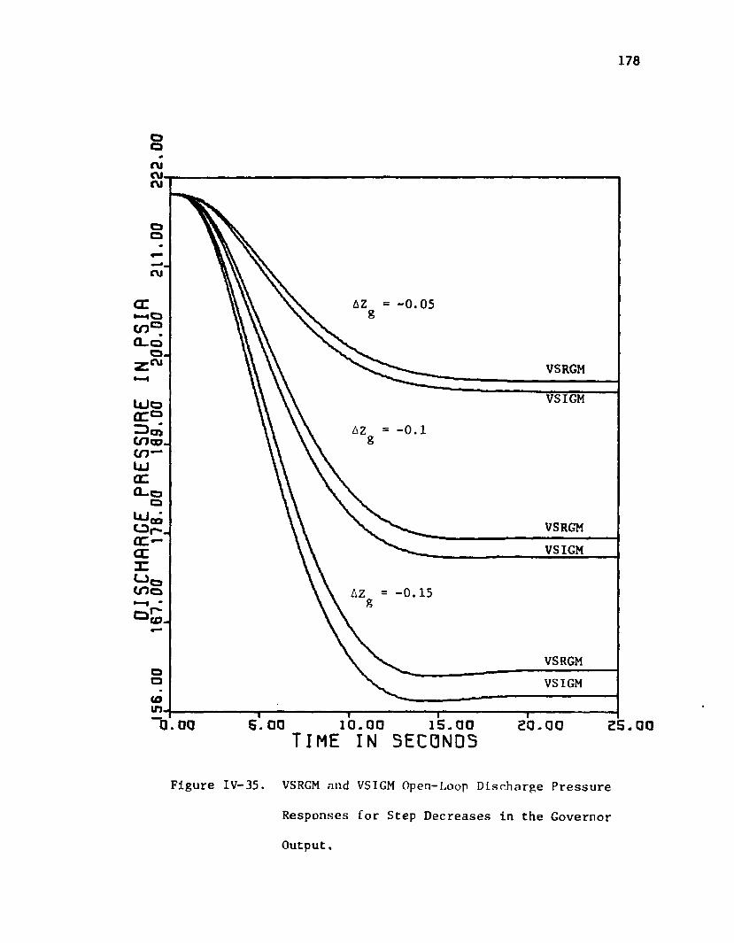
178

oa

rviCMCM

CM

-0.05<X

VSRGM

VSIGM

VSRGMVSIGM

VSRGMQ VSIGMCOm

5 . 00 15.00Q. 00 1 0 . 0 0TIME IN SECONDSFigure IV—35. VSRGM and VSIGM Open—Loop Discharge Pressure

Responses for Step Decreases in the Governor

Output.

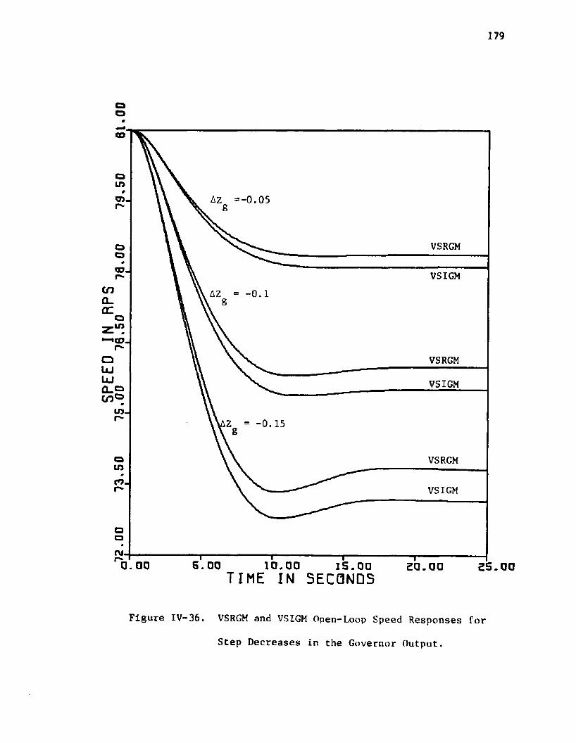
179

oo03

IDAZ =-0.05

VSRGM

VSIGMcn a_acQ

inCD

□LU

VSRGM

VSIGMQ . Oc n °m

in.

VSRGM

VSIGM

ru io.oaTIME IN S EC aNOSFigure IV— 36. VSRGM and VSIGM Open-Loop Speed Responses for

Step Decreases in the Governor Output.

180

and governor output Increases Indicate this trend. It is significant

to note that Increases in the load demand rate produce corresponding

increases in the steam turbine speed. This contradicts the predic

tions which would ordinarily be obtained from an intuitive steady

state analysis. This point illustrates that because of the many

variables which come into play, the compressor-turbine tandem is

very difficult to analyze without a dynamic model.

A unique correlation of the variable speed centrifugal compressor

performance map which reduces the family of head curves to a single

curve has been suggested in terms of reduced head and flow numbers

containing variable exponents. The correlation stems from a dimen

sional analysis of the compressor performance but differs from the

traditional approach which introduces the Mach number to account

for compressibility effects. The proposed correlation accounts

for the compressibility effects with no data required other than the

performance map. It does so by allowing the exponents to take on

the values which collapse the several head curves into a single

curve. A block diagram of the search technique utilized to find

the exponents has been included. The correlation has been success

fully tested for nine different compressors ranging in size from

1900 to 5800 horsepower and in speed from 3000 to 10000 rpm.

Utilizing this correlation, the constant speed compressor

models developed in Chapters II and III have been converted to vari

able speed models. Since the variable speed compressor is integrally

related to its driver, a Jumped parameter dynamic mode] of a steam

181

turbine has also been developed. It was developed in terms of

performance data of an operating steam turbine. The performance

data was received from the General Electric Company. The resulting

variable speed model of the tandem arrangement has been summarized

in an Information flow diagram.

Open loop responses of the variable speed models in terms of

the discharge pressure and the speed have been given in the form of

continuous curves for step disturbances in the compressor inlet

temperature and pressure, the gas molecular weight, the load demand

rate and the steam turbine governor output. These disturbances

indicate that the tandem arrangement possesses many nonlinearities.

They also indicate significant errors between the predictions of

the model based on the ideal gas law and the model based on the

MBWR equation of state.

It is felt that with these models, the steam turbine manufac

turer can develop more efficient governor mechanisms that those

utilized in industry today. Also, the control engineer can utilize

them to develop advanced control systems which are capable of

delivering adequate control at all levels of operation of the tandem.

Possibly the astute control engineer can even develop a suitable

control scheme for starting up the system automatically.

182

NOMENCLATURE

A — constant In parabolic head equation

a - exponent In reduced head number

B - constant in steam turbine performance equation

b - exponent in reduced flow number

F - mass flow rate, lbm/sec

FC - flow controller

FX - flow transmitter

8c - 32.2 lbm-ft/lbf-sec2

H - head, ft-lbf/lbm

h - molar enthalpy, BTU/lb-mole

I - inertia, lbm-ft2

Kt - constant in steam turbine performance equation

L - steam turbine load, hp

LLS - linear least squares

M - molecular weight, lbm/lb-mole

N - speed, rps

NLS - nonlinear least squares

P - pressure, psia

PC - pressure controller

PX - pressure transmitter

Q - volumetric flow rate, acfs

T - temperature, °F; torque, ft-lbf

W _ steam rate, lbm/hr

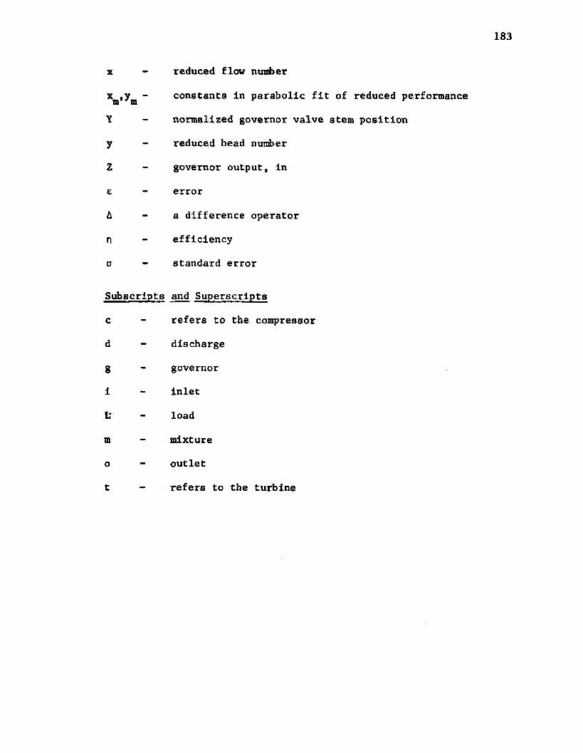
x - reduced flow number

x ,y - constants In parabolic fit of reduced performancem mY - normalized governor valve stem position

y - reduced head number

Z - governor output, in

e - error

A - a difference operator

D - efficiency

0 - standard error


c - refers to the compressor

d - discharge

g - governor

1 - inlet

L" - load

m - mixture

o - outlet

t - refers to the turbine

184

LITERATURE CITED

1. Hancock, R., "Drivers, Control and Accessories," Chemical Engineering, (June 1956), pp. 227-238.

2. Bresler, S. A., "Prime Movers and Process Energy," Chemical Engineering, (May 23, 1966), pp. 124-144.

3. Steen-Johnson, H., "Mechanical Drive Steam Turbines," Hydrocarbon Processing, (October 1967), pp. 126-130.

4. Farrow, J. F., "User Guide to Steam Turbines," Hydrocarbon Processing, (March 1971), pp. 71-75.

5. Wilson, W. B. and Hiniker, T. G., "Integrating Gas Turbines into Process Systems," presented at the General Electric Gas Turbine State of the Art Engineering Seminar, June 1967.

6 . Wilson, W. B., "Gas Turbine Energy Systems for the Process Industries," presented at the General Electric Gas Turbine State of the Art Engineering Seminar, September 1970.

7. Moens, J. P. C., "Adapt Process to Compressor," Hydrocarbon Processing, (Dec. 1971), pp. 96-100.

8 . Corrigan, T. E. and Johnson, A. F., "How Speed Affects Performance," Chemical Engineering, (Feb. 1954), pp. 209-210.

9. Nisenfeld, A. E., Marks, A. F. and Schultz, H. M., "Analog Simulation as an Aid in Control System Design," Proceedings of the 1971 Summer Computer Simulation Conference, Boston, Mass. (July 1971), pp. 324-330.

10. Jeffrey, D. K., "Investigation into Anti-surge Control of an Air Compressor," The South African Engineer, (April 1971), pp. 37-48.

11. Bergeron, E. P. and Corripio, A. B., "Simulation of Start-Up of an Industrial Refrigeration System," Proceedings of the 1971 Computer Simulation Conference, Boston, Mass. (July 1971),pp. 306-315.

12. Franks, R.E.G., Modeling and Simulation in Chemical Engineering, Wiley-Interscience, N. Y., 1972, pp. 376-391.

13. Shepherd, D. G., Principles of Turbomachinery, MacMillan Co., N.Y. N.Y., 1956, Chapter 2.

14. Csanady, G. T., Theory of Turbomachines, McGraw-Hill Book Co.,New York, 1964, Chapter 1.

185

15. Moore, C. F., Smith, C. L. and Murrill, P. W., "Multidimensional Optimization Using Pattern Search," Share Program Library. Program Number SDA-3552, September 1968.

16. Cutter, W. C., Private Communication, March 23, 1972.

17. Rowen, W. I., Private Communication, December 27, 1971.

CHAPTER V

CONCLUSIONS AND RECOMMENDATIONS

The purpose of this study has been to develop dynamic models of

large industrial centrifugal compressors, ones that require only the

data developed by the manufacturer and which accompanies the machines.

In this chapter, the conclusions drawn from the results presented in

the previous chapters are summarized and recommendations for future

research efforts are given.

The development of a dynamic model of the constant speed compres

sor utilizing the ideal gas law along with both open and closed loop

simulation results were given in Chapter II. The open loop results in

dicated that the constant speed machine is very nonlinear. The char

acteristic time of the process was found to be strongly dependent upon

the magnitude and direction of change of each of the load distrubances:

changes in the inlet pressure, inlet temperature, gas molecular weight,

and load demand rate. The system time constant, gain and dead time

obtained from process reaction curves were found to be extremely

sensitive to changes in the governor output. It was vividly demon

strated that tuning constants optimally determined through utilization

of the nonlinear model yield far superior responses for the load dis

turbances than do those obtained from a conventional tuning technique.

In Chapter III, the modifications required to account for the

nonidealities of the gas were given in terms of a modified Benedict-

Webb-Rubin equation of state. Open and closed loop simulation results

186

187

utilizing the modified model, the CSRGM, were obtained and com

pared with those of Chapter II* A comparison of the open loop

results indicated that the assumption of an ideal gas may introduce

significant errors. The same dependence of the characteristic time

upon the magnitude and direction of change of the disturbance was

found for changes in inlet pressure and load demand rate while an

opposing dependence was found for changes in inlet temperature and

molecular weight. Each of the parameters taken from the process

reaction curves obtained from the CSRGM were larger than those of

Chapter II but their trends were the same.

The modifications required to convert the two constant speed

models to variable speed models along with the development of a steam

turbine model were given in Chapter IV. Open loop responses obtained

from the resulting two models indicated that the variable speed

centrifugal compressor is even more nonlinear than the constant speed

one. These responses also indicated that the assumption of an ideal

gas introduces errors which are more significant for the variable

speed model than they are for the constant speed model.

Future research efforts regarding the simulation of the centri

fugal compressor should be directed toward ascertaining the predictions

of the models given here which can only result from a comparison with

an actual machine. It is quite possible that these models do not

adequately represent the actual machine but that a modification such

as adding a discharge energy balance, utilizing an efficiency which

is dependent on volumetric flow rate rather than a constant value or

distributing the suction and discharge systems by adding resistance

terms may bring them in line with real life conditions.

188

If It Is found that the models adequately represent the actual

compressor system then future research efforts should be directed

toward modeling the multistage machine. A model capable of handling

composition changes at the inlet of the system should also be investi

gated. Efforts should be made to determine if it is feasible to lump

the suction and discharge volumes into a single volume. Should this

be the case the model would be greatly simplified as the volumetric

flow rate could then be determined directly rather than indirectly.

Also, a convenient method for describing the surge of the compressor

via a digital model is urgently needed.

In the area of process control, research is needed to adequately

characterize the compression process in terms of the design parameters.

With such a characterization the advanced control concepts such as

adaptive tuning could be investigated. For the simple plant such

as utilized in this study, research should be directed toward develop

ing a multivariable control system, one capable of preventing excur

sions into the surge region even for decreased throughputs and at

the same time providing adequate discharge or suction pressure control.

Finally, research efforts should be directed toward developing nonlinear

control systems, ones capable of providing adequate control at all

levels of operation. With this the compressor could be started up

automatically.

APPENDIX A

STEADY STATE DESIGN OF THE PLANT

190

Design Basis: The steady state design Is based on propane being

In the Ideal gas state. The operating conditions have been

chosen very near to those for which the compressor was

originally designed. However, enough deviation has been

included so that the possibly restricted details of the pro

cess for which the compressor was designed would not be

revealed.

A. STEADY STATE OPERATING CONDITIONS

Tfl - 70°F - 530°R

Pg ■ 75 psia

p„ - 0.581414 lbm/ft3

Td « 109°F = 569°R

Pd ■ 220 psla

pd = 1.58858 lbm/ft33Qc ■ 17597 ft /mln @ suction conditions

H - 19970 ft-lbf/lbm

W ■ 10231 lbm/mln

B. DESIGN OF PIPING

An estimate of the piping size Is obtained through application

of the mechanical energy balance for the steady flow of an In

compressible fluid through a horizontal length of pipe. Even

though the fluid is compressible the incompressible equation

is used because the pressure drop will be limited to a maxi

mum of 2 psi/1 0 0' of pipe and Isothermal flow is assumed.

The equations utilized are

191

AP - (4.8A f w 2)/(pd5)

Re * (380w)/(dy)

where

d * Inside pipe diameter, Inch

f * friction factor

AP = pressure drop, psi/100'

Re * Reynolds number

p «* density, lbm/ft^

w = flow rate, lbm/min.

The values for f, y, and the surface roughness factor e were

obtained from the fourth edition of Perry's Chemical Engineers

Handbook, y from page 3-147, e from page 5-19 and f from

page 5-20.

1. Suction Piping

@ the suction conditions y * 0.008 cp

Assuming a pipe diameter of 20"

Re - (380 x 1023)/(20. x 0.008) = 2.5 x 10?

For commercial steel pipe e/d = 0.0001

At this value of Re and e/d, f » 0.003

AP = (4.84 x 0.003 x 102312)/(0.581414 x 20.5)

- 0.93 psi/100'

In a similar manner the following values of pipe size were

obtained for the Indicated pressure drop.

Line Diameter 18" 20" 24"

AP/100' 0.4 0.93 1.91

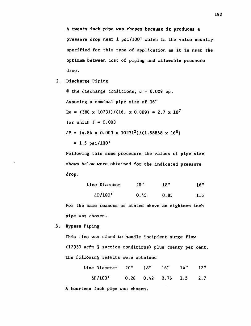
A twenty inch pipe was chosen because it produces a

pressure drop near 1 psi/1 0 0' which is the value usually

specified for this type of application as it is near the

optimum between cost of piping and allowable pressure

drop.

Discharge Piping

@ the discharge conditions, p = 0.009 cp.

Assuming a nominal pipe size of 16"

Re = (380 x 10231)/(16. x 0.009) = 2.7 x 107

for which f = 0.003

AP = (4.84 x 0.003 x 102312)/(1.58858 x 165)

= 1.5 psi/100'

Following this same procedure the values of pipe size

shown below were obtained for the indicated pressure

drop.

Line Diameter 20" 18" 16"

AP/100' 0.45 0.85 1.5

For the same reasons as stated above an eighteen inch

pipe was chosen.

Bypass Piping

This line was sized to handle incipient surge flow

(12330 acfm @ suction conditions) plus twenty per cent.

The following results were obtained

Line Diameter 20" 18" 16" 14" 12"

AP/100' 0.26 0.42 0.76 1.5 2.7

A fourteen inch pipe was chosen.

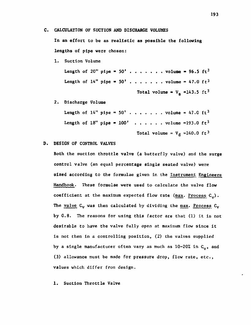
193

C. CALCULATION OF SUCTION AND DISCHARGE VOLUMES

In an effort to be as realistic as possible the following

lengths of pipe were chosen:

1. Suction Volume

Length of 20" pipe = * 5 0 ' ............... volume = 96.5 ft3

Length of 14" pipe " 5 0 ' volume = 47.0 ft3

Total volume = Vs =143.5 ft3

2. Discharge Volume

Length of 14" pipe = 5 0 ' ............... volume = 47.0 ft3

Length of 18" pipe = 1 0 0 ' ............. volume =193.0 ft3

Total volume = Vj =240.0 ft3

D. DESIGN OF CONTROL VALVES

Both the suction throttle valve (a butterfly valve) and the surge

control valve (an equal percentage single seated valve) were

sized according to the formulae given in the Instrument Engineers

Handbook. These formulae were used to calculate the valve flow

coefficient at the maximum expected flow rate (max. Process Cv) .

The valve Cv was then calculated by dividing the max. Process Cy

by 0.8. The reasons for using this factor are that (1) it is not

desirable to have the valve fully open at maximum flow since it

is not then in a controlling position, (2) the valves supplied

by a single manufacturer often vary as much as 10-20% in Cv , and

(3) allowance must be made for pressure drop, flow rate, etc.,

values which differ from design.

1. Suction Throttle Valve

194

Utilize the procedure given by Moore^ for compressor

throttle valves, take the valve pressure drop as 5% of the

suction pressure.

Max. Process Cy = F^/Cl.05 v pAPv)

APV = 0.05 Pg = 3.75 psia which was rounded up to 4 psia.

Utilize the average of the up- and downstream densities.

p = 0.5 (p + p g )

Pl= PiM/RTi =(79 x 44.09)/(10.731 x 530)

- 0.611089 lbm/ft3

p - (0.611089 + 0.581414)0.5 - 0.59625 lbm/ft3

Design the valve to handle the flow at the "stonewall"

(the maximum possible flow rate) at the above APv and p .

"stonewall flow" = 21300 ft3/min x 0.581414 lbm/ft3

Max. Process Cv = 7633 lbm/min.

Valve Cv = 7633/0.8 = 9541 lbm/min.

This requires a 20" valve.

2. Surge Control Valve

Size this valve to handle 120% of surge flow utilizing the

design equation for critical flow.

5.1 Fe ^Tp Max. Process C„ = 7;— 5—-------------v Cf Pe 3T

Assume the cooler maintains the outlet temperature at

l-Moore, R. W., "Allocating Pressure Drops to Control Valves," Instrumentation Technology, (Oct. 1970), pp. 102-105.

195

530°R and that the pressure drop across the cooler is

3 psi at the maximum flow rate:

F - 1.2 x 12330 acfm x 0.581414 lbm/ft3 - 8602.6 lbm/min.

P = 217 psia eT - 530°R eCf = 0.9

Max. Process = 779 lbm/min

Valve C = 779./0.8 =974 lbm/min vThis requires a 10" valve.

APPENDIX B

IMPLICIT LOOP SOLVING ROUTINES

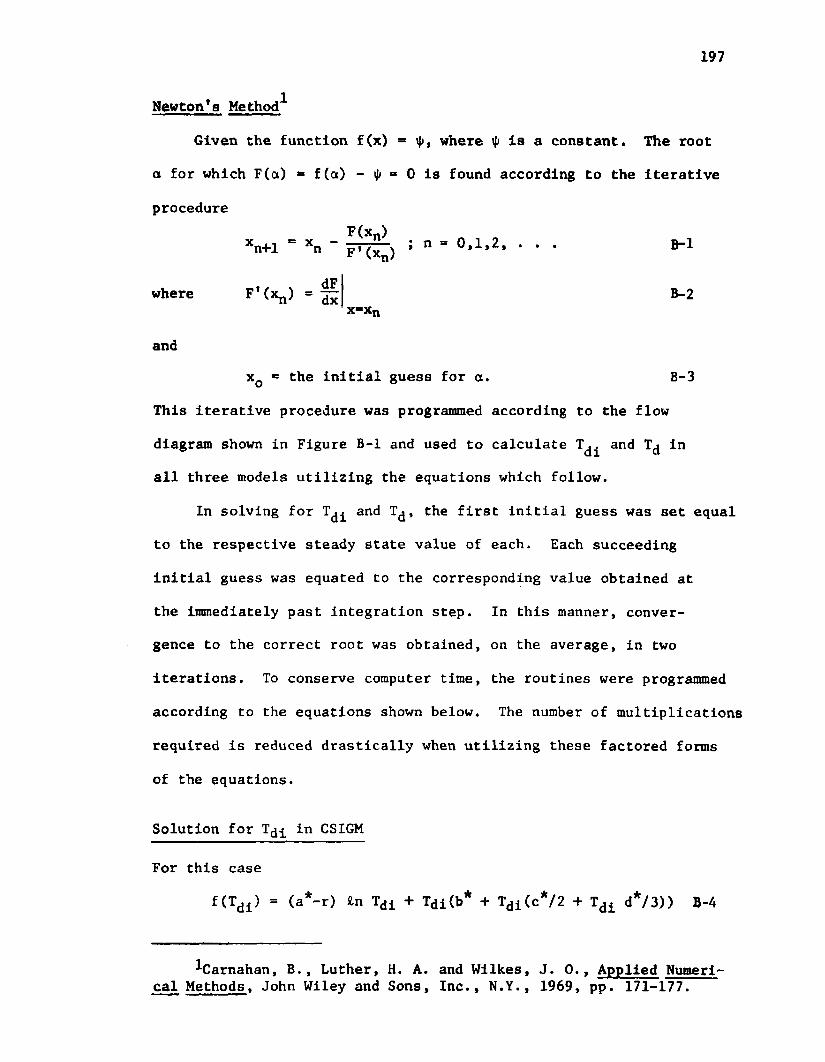
197

Newton’s Method*

Given the function f(x) = >|>, where i|i is a constant. The root

a for which F(a) = f(a) - 4> “ 0 is found according to the iterative

procedure

This iterative procedure was programmed according to the flow

diagram shown in Figure B-l and used to calculate and Td in

all three models utilizing the equations which follow.

In solving for and Td , the first initial guess was set equal

to the respective steady state value of each. Each succeeding

initial guess was equated to the corresponding value obtained at

the immediately past integration step. In this manner, conver

gence to the correct root was obtained, on the average, in two

iterations. To conserve computer time, the routines were programmed

according to the equations shown below. The number of multiplications

required is reduced drastically when utilizing these factored forms

of the equations.

Solution for Td^ in CSIGM

For this case

x=xnB-2

B-l

andxQ = the initial guess for a. B-3

f(Tdi) = <a*-r) fcn Tdi + Tdi(b* + Tdi(c*/2 + Tdi d*/3)) B-4

^■Carnahan, B., Luther, H. A. and Wilkes, J. 0., Applied Numerical Methods, John Wiley and Sons, Inc., N.Y., 1969, pp. 171-177.

198

Entry with x0

x=x

F (x)““X' F 0 0

Falsea-xx=a

True

Exit with a

Figure B-l. Computer Flow Diagram for Newton's Method for Solving Implicit Functions.

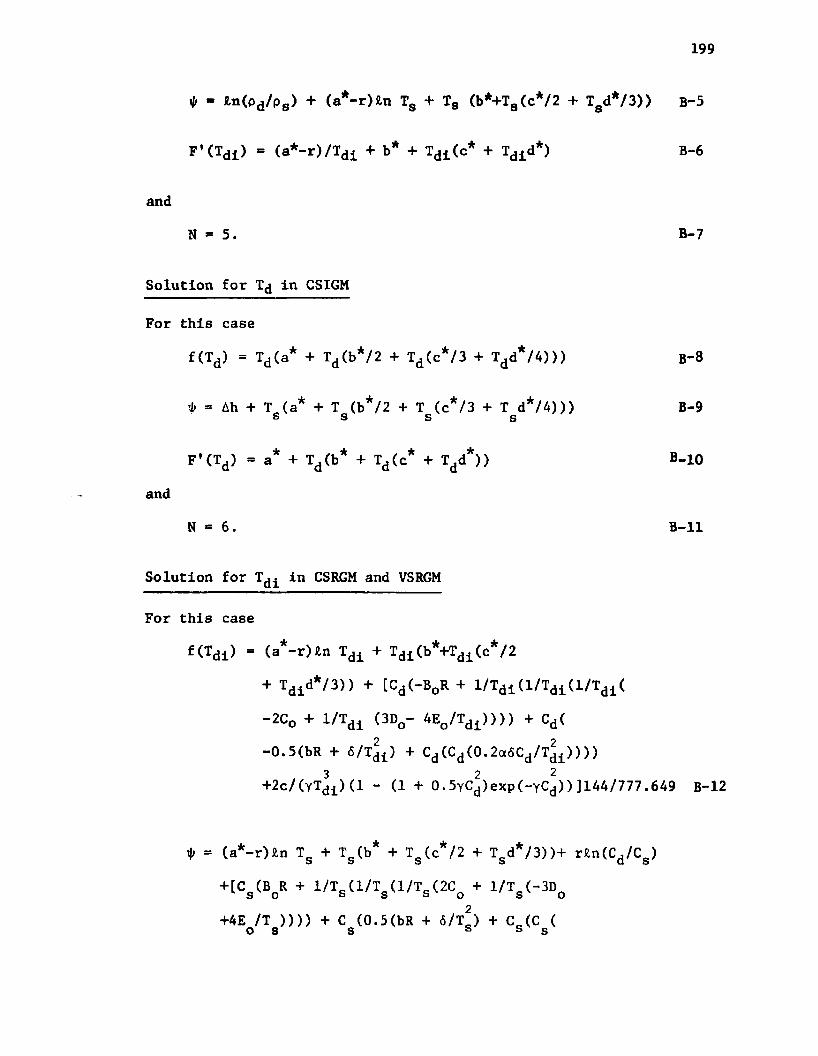
* - Jtn(pd/ps) + (a*-rHn Tg + Ts (b*+Ts(c*/2 + Tgd*/3))

F'(Tdl) = (a*-r)/Tdl + b* + Tdl(c* + Tdjd*)

and

N * 5.

Solution for Td in CS1GM

For this case

f(Td) = Td (a* + Td (b*/2 + Td (c*/3 + Tdd*/4)))

'i> = Ah + T (a* + T (b*/2 + T (c*/3 + T d*/4))) s s s s

F ’(Td) = a* + Td (b* + Td (c* + Tjd*))

and

N - 6.

Solution for Tdi in CSRGM and VSRGM

For this case

f(Tdi) - (a*-r)£n Tdi + Tdl(b*+Tdi(c*/2

+ Tdld*/3)) + [Cd (-B0R + 1/Tdi(l/Tdi(l/Tdi(

-2C0 + 1/Td± (3Dq- 4EQ/Tdl)))) + Cd(

-0.5(bR + S/Tdi) + Cd(Cd(0.2a6Cd/Tdi))))3 2 2

+2c/(yTdi)(l - (1 + 0.5yCd)exp(-yCd))]144/777.649 B-12

* = (a*-r)Jln Tg + Tg(b* + Ts(c*/2 + Tgd*/3))+ r*n(Cd/Cg)

+[C ( B R + 1/T (1/T (1/T (2C + 1/T (-3DS O ° S ° O 5 0

+4E /T )))) + C (0.5(bR + 6/T*) + C (C ( o s s s» s g

199

B-5

B-6

B-7

B-8

B-9

B-10

B-ll

200

-0.2 a6Cs/Tg)))) - 2c/(yTg)(l-(l +

0.5yCg) exp (-YCg))]144./777.649 B-13

F'(Tdl) - (a*-r)/Tdi + b* + Tdi(c* + Tdid*) + ]Cd (

l/Tdi(l/Tdi(l/Tdi(l/Tdi(6C0+l/Tdi(-12D0

+ 20EQ/Tdi))))) + Cd (6/Tdi + Cd (Cd(

1 + 0.5YCd)exp(-YCd))]144./777.649and

N - 5.

Solution for Td in CSRGM and VSRGM

For this case

f(Td)= {Cd [B0RTd - 2Aq + 1/Td(l/Td (-4C0+1/Td (

5Dq - 6E0/Td))) + Cd [bRTd - 1.5a - 26/Td

+ Cd [Cd [0.2ct(6a + 76/Td)Cd]]]]2 2 2 4 2

+ c/(YTd)(3-(3 + 0.5YCd - y Cd)exp(-YCd))}144./777.649 + Td (a* + Td (b*/2 + Td (c*/3 + Tjd*/4))) B-16

* " {cs[BoRTs " ^ o +1/Ts(1 /Ts ("4Co + 1/Ts (5Do -6E0 /Tg))) + Cg[bRTg - 1.5a-25/Tg + Cg [Cs [

0.2a(6a + 76/Ts)Cg]]]] + c/(YTg)(3-

(3 + 0.5YC?-Y2C*!)exp(-YCj)}l44./777.649S S o+ Ts(a* + Tg (b*/2 + Ts(c*/3 + Tgd*/4))) + h B-l 7

F ’(Td) = (Cd [BoR + l/Td(l/Td (l/Td (8C0 + 1/Td<

-15Do + 24Eo/Td)))) + Cd [bR + 26/T* +

Cd [ Cd [ -1.4«4Cd / 'Td 2 ] ] ] ] - (2c /y Tj) (3

B-14

B-15

201

and

N - 6 .

-(3 + 0.5yC^-Y2C^)exp(-YCj))}l44./777.6A9 + a* + Td (b* + Td (c* + Tdd*))

B-18

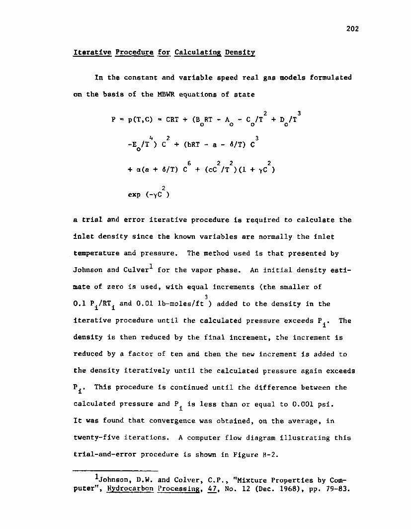
202

Iterative Procedure for Calculating Density

In the constant and variable speed real gas models formulated

on the basis of the MBWR equations of state

2 3P = p(T,C) » CRT + (B RT - A - C /T + D /To o o o* ♦ 2 3

-E /T ) C + (bRT - a - fi/T) C o6 2 2 2

+ a(a + 6/T) C + (cC /T )(1 + yC )

2exp (-yC )

a trial and error iterative procedure is required to calculate the

inlet density since the known variables are normally the inlet

temperature and pressure. The method used is that presented by

Johnson and Culver^- for the vapor phase. An initial density esti

mate of zero is used, with equal increments (the smaller of3

0.1 P^/RT^ and 0.01 lb-raoles/ft ) added to the density in the

iterative procedure until the calculated pressure exceeds P^. The

density is then reduced by the final increment, the increment is

reduced by a factor of ten and then the new increment is added to

the density iteratively until the calculated pressure again exceeds

P^. This procedure is continued until the difference between the

calculated pressure and is less than or equal to 0.001 psi.

It was found that convergence was obtained, on the average, in

twenty-five iterations. A computer flow diagram illustrating this

trial-and-error procedure is shown in Figure B-2.

^Johnson, D.W. and Colver, C.P., "Mixture Properties by Computer", Hydrocarbon Processing, 47, No. 12 (Dec. 1968), pp. 79-83.

Entry with Tj.Pj.M

0 > >0DR - 0.01

=0

_3P-P 10

P<P =0P-Pi

Ci= 0

Delta = DR

Delta=0.01

P=p(T.,C.)

Delta = Delta/10.

Figure B-2. Trial and Error Procedure forthe Inlet Density.

APPENDIX C

PROCESS REACTION CURVES

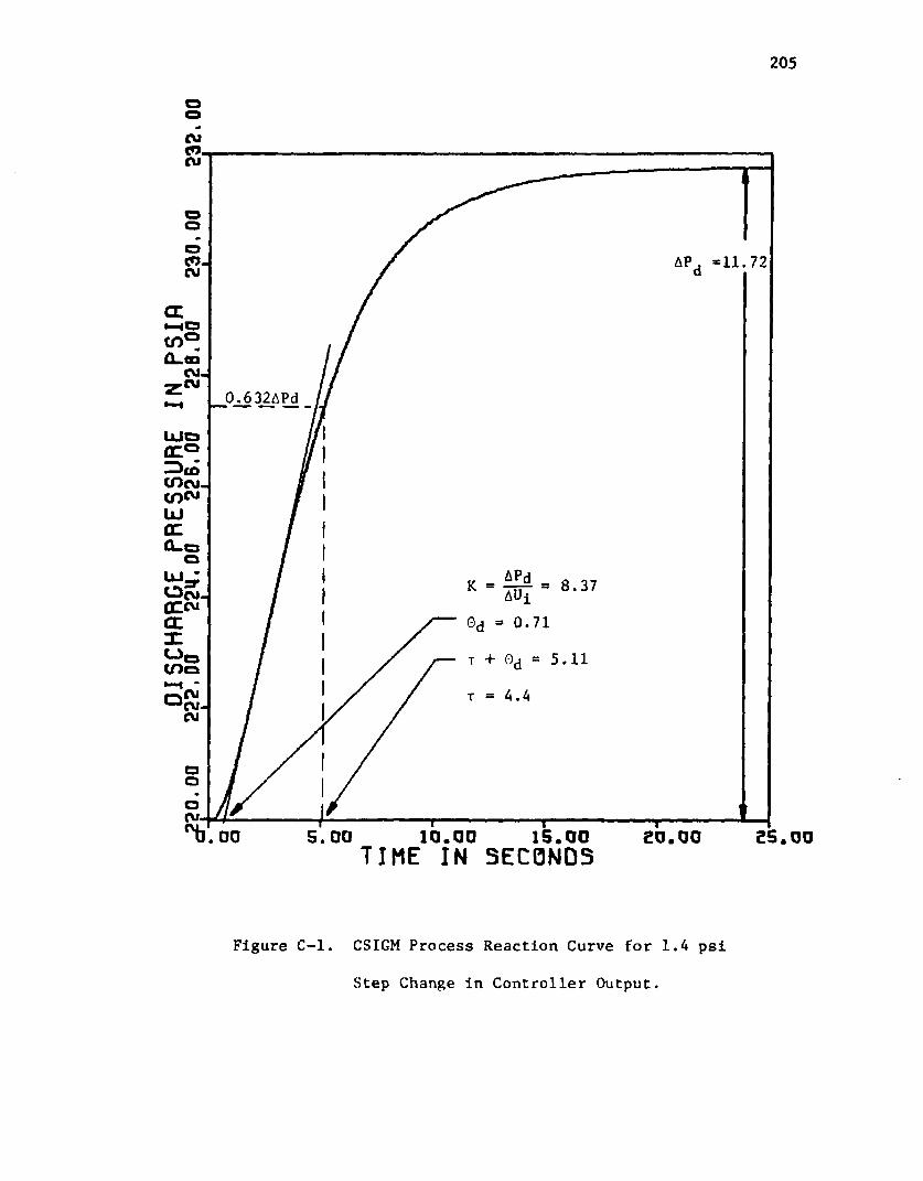
205

COru

AP , *11.72

<X

5.11•— < - u cuCM

15.005.00 10.0000 TIME IN S EC O N D S

Figure C-l. CSIGM Process Reaction Curve for 1.4 psi

Step Change in Controller Output.

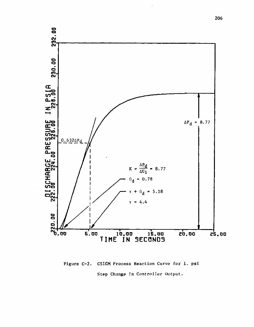
206

cncm

cn.CM

8.77AP,

OcC.GQCM

I01'cm.CM

oCM.

E. 000 0 15.0010.00TIME IN SECONDS

Figure C-2. CSIGM Process Reaction Curve for 1. psi

Step Change In Controller Output.

207

CM.CM

A. 81

CM-CU

orvj

15.00DO 25.00TIME IN S EC O N D S

Figure C-3. CSIGM Process Reaction Curve for

0.5 psi Step Change in Controller

Output.

01SCH

RRGE

PRES

SURE

IN

PSIfl

.220

.00

220.

50

221.

00

221.

50

222.

00

222.

50

223.

00trl

I I

i i

■ a

208

0.632 APd

APd — - = 10.2 AUi1 0. 84

5. 0 0 1 5 . 0 0.00 10.00TIME IN S EC O N D SFigure C-4. CSIGM Process Reaction Curve for

0.25 psi Step Change in Controller

Output.

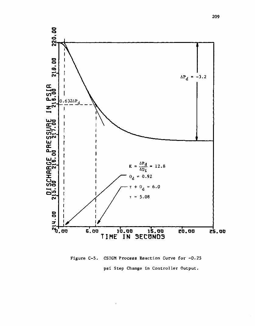
209

CDCM -3.2AP

CEm oC O ®a. cd 632AP

CM

nr cm .^!4- 12.8AUi = 0.92

5.08CM

o

=rG. 00 1 5 . 0 010.0000 TIME IN S EC O ND S

Figure C-5. CSIGM Process Reaction Curve for -0.25

psi Step Change in Controller Output.

DISC

HARG

E PR

ESSU

RE

IN PS

IR,2

06.0

0 21

0.00

21

2.00

21

U.00

21

6.00

21

6.00

22

0.00

U I

I I

f a

i ■

210

0.96

6.38

S. 00 15.0010.00TIME IN S ECONDS

Figure C-6. CSIGM Process Reaction Curve for -0.5 psi

Step Change in Controller Output.

211

cuCM

CD AP. = -17.77CM

CL

632AP

O 1.05CM

IDat.

G .00 15.000 0 1 0 . 0 0TIME IN SECONDS

Figure C-7. CSIGM Process Reaction Curve for -1.0

psl Slop Change In Controller Output.

212

O

CM.CM

U)AP. = -29.75CM

APdK = — - = 21.25AUj

o

O)15.005.00 10.00TIME IN 3 EC 0N05

Figure C-8 . CSIGM Process Reaction Curve for -1.4

psi Step Change in Controller Output.

DISC

HARG

E PR

ESSU

RE

IN PS

IR<£

17.0

0 22

0.00

22

3.00

2£

6.00

22

9.00

23

2.00

23

5.00

213

0.632 AP

AP 14.37

APdK = — - = 10.26 AUiOd = 1-02

5.83

4.81

J

15.005.00 10 .00. DO 20.00TIME IN SECONDS

Figure C-9. CSRGM Process Reaction Curve for 1.4 psi Step Change in Controller Output.

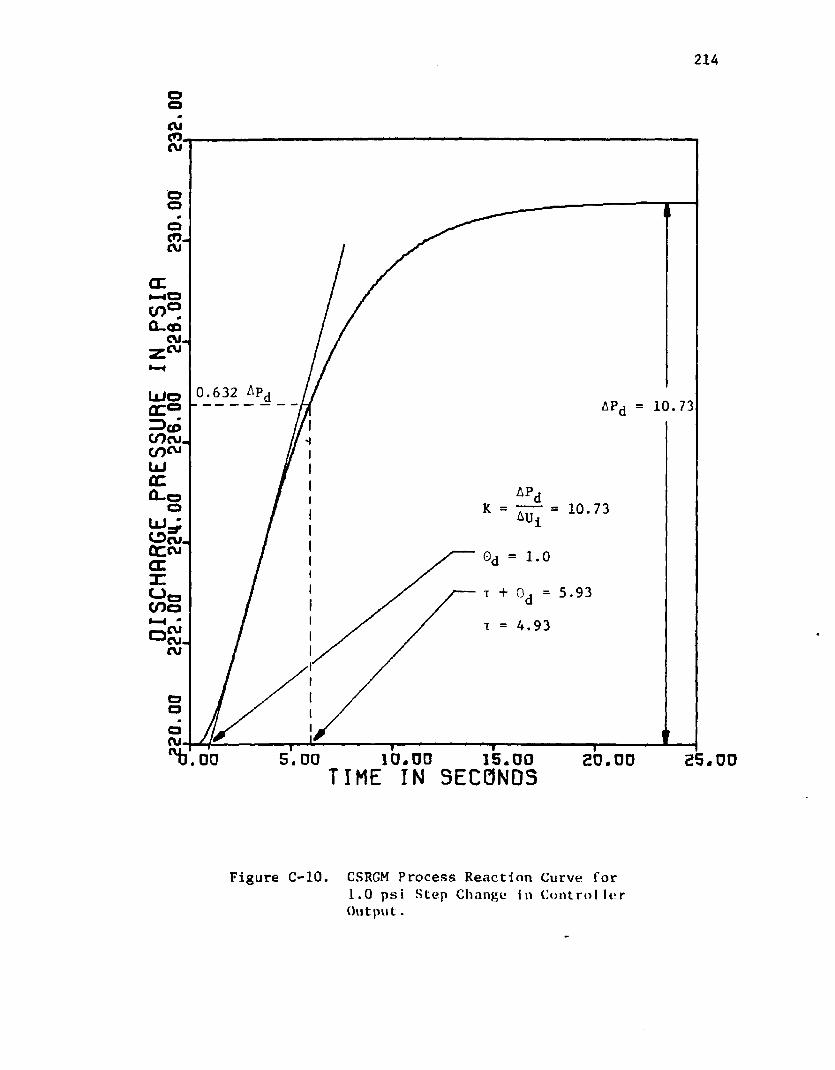
OISC

HRRG

E PR

ESSU

RE

IN PSI

fl^2

20.QO

22

2.00

22

4.00

22

6.00

22

6.00

23

0.00

23

2.00

Cr i

i i

i j

i i

214

0.632 Ap;10.73AP

AP10.73

5.00 15.00.00 20.00TIME IN SECONDS

Figure C-10. CSRGM Process Reaction Curve for1.0 psi Step Change in ControllerOutput.

.00

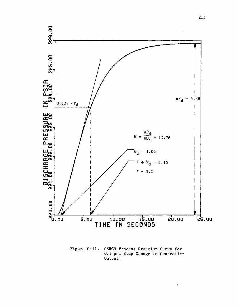
215

CDCU,CVJ

O

CL

5.88AP0.632 AP

LUOflC°^>cr>COcuLUorQ - o

AP,11.76

1.05

6.15

O mcv»

ru15.00 25.005.00 20.001 0 .0 00 0 TIME IN SECONDS

Figure C-ll. CSRGM Process Reaction Curve for0.5 psi Step Change in ControllerOutput.

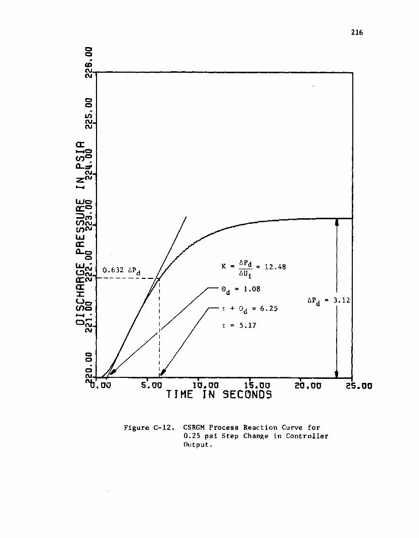
OISC

HRRG

E PR

ESSU

RE

IN PS

IR<-

220.

00

221.

00

222.

00

223.

00

224.

00

225.

00

226.

00U

| I

| |

I I

I

216

= 12.48AU.0.632 AP

1.083.12AP

5.17

5.00 15.0010 .0000 20.00 25.00TIME IN SECONDS

Figure C-12. CSRGM Process Reaction Curve for0.25 psi Step Change in ControllerOutput.

217

oooCVI,CVI

05

&Pd = -3.89

632 AP,

CLQ - o

= 15.56

1.14

15.005.00 25.0010 .00 20.0000 TIME IN S ECONDS

Figure C-13. CSRGM Process Reaction Curve for-0.25 psi Step Change in ControllerOutput.

DISC

HRRG

E PR

ESSU

RE

IN PS

IR.2

08.0

0 21

0.00

21

2.00

21

4.00

21

6.00

21

6.00

22

0.00

U I

I I

J I

I

218

17.52

7.18

5.96

15.00 25.0000 10 .00TIME IN SECONDS


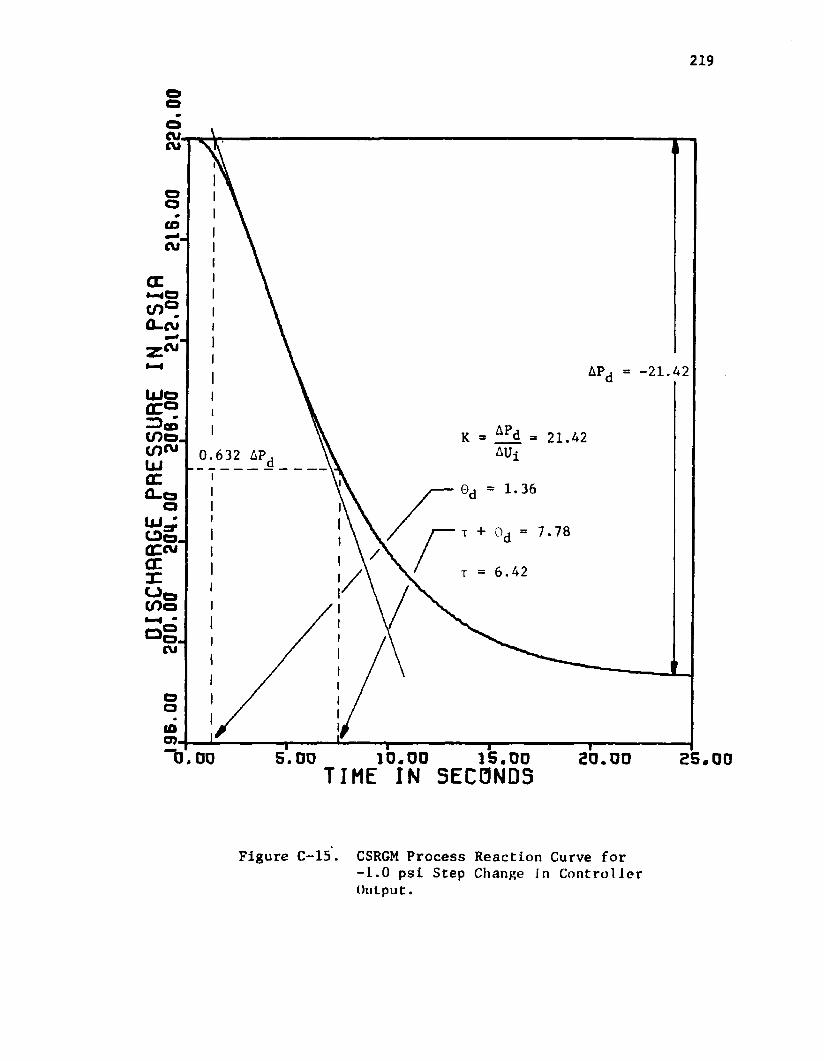
219

ocu.CM

CDCM

CCH Ot n ®Q-cviZ ™

APj = -21.42U J oQ T OZ3goCOO.LU

= 21.42AUi632 AP

1.36

7.78

6.42o 0COoo

CM

o

CD.5.00 15.0000 1 0 .0 0TIME IN SECONDS


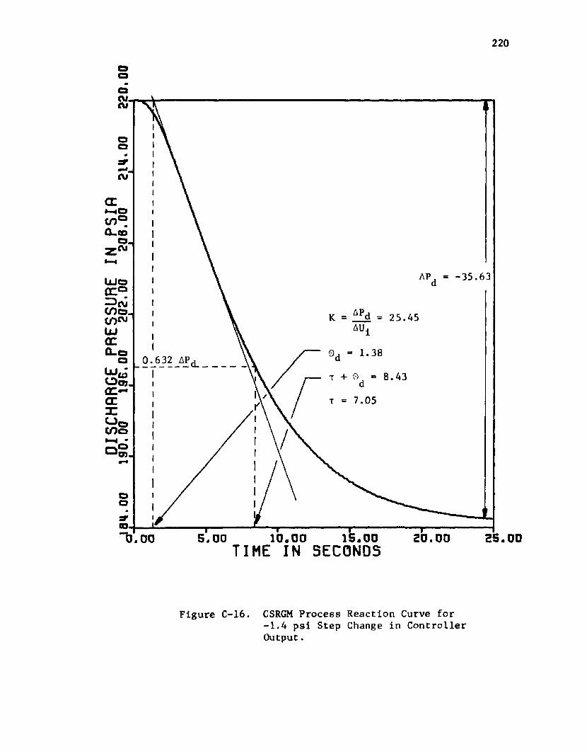
DISC

HRRG

E PR

ESSU

RE

IN PS

IR—1

84.0

0 19

0.00

19

6.00

20

2.00

20

6.00

21

H.00

22

0.00

CJ I

I ■

J J

1 I

220

AP, = -35.63

AP,AU

25.45

1.38632 AP8.43

7.05

20.0010.0000 TIME IN SECONDS


APPENDIX D

THERMODYNAMIC DERIVATIONS

This appendix has been Included to provide the derivations

of the thermodynamic equations needed to calculate the changes in

the molar entropy, molar enthalpy and the molar internal energy

when the equation of state relates pressure as a function of

temperature and molar density. The derivations are based on one

mole and, up to the point at which the particular equation of state

is utilized, are completely general. They are applicable for the

closed system.

Consider the following change of state which is accompanied

by the indicated general thermodynamic property change:

State A A6 State B

Propose the following reversible path:

<CA »TA> (0*ta) A0H (0,Td) _^IIi.(CB ,TB)

for which

A0 - AGj. + A©it + A0m . D-l

Entropy Change Derivation

Utilizing equation D-l, the molar entropy change accompanying

the change in state is given by

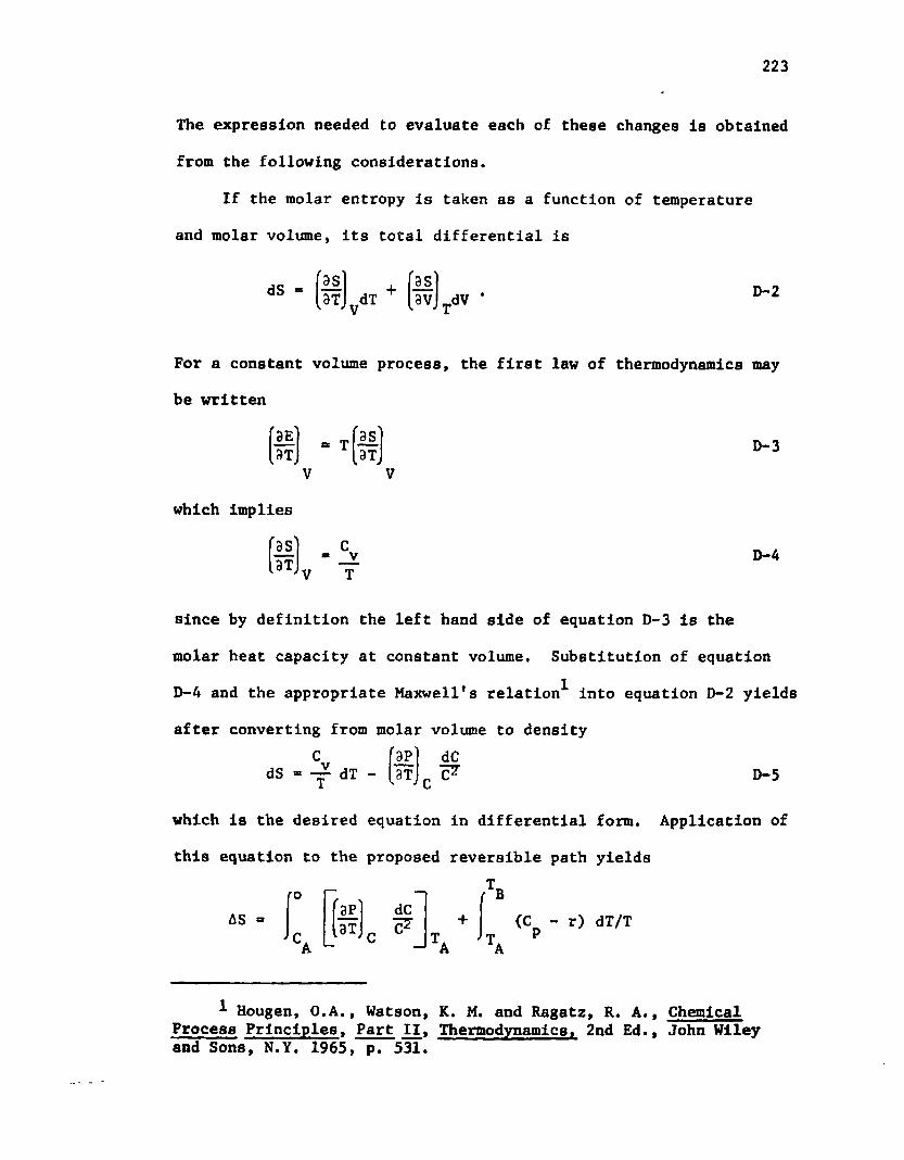
223

The expression needed to evaluate each of these changes Is obtained

from the following considerations.

If the molar entropy is taken as a function of temperature

and molar volume, its total differential is

dS 'as' J.3T\ vdT

asavlTdV * D-2

For a constant volume process, the first law of thermodynamics may

be written

3E B T3T m 1 as

3T D-3

which implies

= _v V T

D-4

since by definition the left hand side of equation D-3 is the

molar heat capacity at constant volume. Substitution of equation

D-4 and the appropriate Maxwell's relation’*' into equation D-2 yields

after converting from molar volume to density

dS = dT -ap3T

dCC* D-5

which is the desired equation in differential form. Application of

this equation to the proposed reversible path yieldsT„

AS 9P3T

dCC*

B(C - r) dT/T P

1 Hougen, O.A., Watson, K. M. and Ragatz, R. A., Chemical Process Principles, Part II, Thermodynamics, 2nd Ed., John Wiley and Sons, N.Y. 1965, p. 531.

224

tel i g l[btJ c7— r —I'

D-6

where the substitution C = C + r has been made in the secondP vintegral since this relation holds for an ideal gas. It should

be noted that the first integral is AS^, the second ASj^ and the

third is AS

The equation of state utilized in this study is the modified

BUR equation of state developed by Starling*-

P - CRT + (B RT - A - C /T2 + D /T3 o o o o

- Eo/T4)C2 + (bRT - a - 6/T)C3

+ ct(a+6/T)C6

+ U + yC2)exp(-yC2), D-7

Utilizing this equation, the change in pressure with temperature

at constant density is

3P3T CR + (B R + 2C /T3 - 3D /T*4 + 4E /T5)C2 o o o o '

+ (bR + 6/T2 )C3 - a6C6/T2

2cC; (1 + yC2 )exp(-yC2). D-8

The relation utilized in this study to calculate the molar heat

^-Starling, K.E. "Thermo Data Refined for LPG", Hydrocarbon Processing, (Mar. 1971), pp. 101-104.

225

2capacity is that proposed by Thinh, etal. which has the form* * * „ * QC - a + b T + c T2 + d T 3. D-9P

Substitution of equations D-8 and D-9 into equation D-6 yields

after integration

as - <cASj(ta) + c2s2(ta) - c|s3(ta)

- s„(ta>ca) - cbs,(tb) - c=s2<tb)

+ C=S3(Tb) + S,,(Tb ,Cb)} 144./777.649

+ Sid(TB'CB) - Sid(TA"CA> B - 10

144where --- *■. is a factor to convert from the mechanical energy777.649units (psia-ft3/lb-mole) to the thermal energy units (BTU/lb-mole)

and the indicated functions have been defined for convenience and

are

Si(T) - B R + 2C /T3 - 3D + 4E /T5 D-ll1 o o o o2

S2 (T) =0.5 (bR + 6/T ) D-12

S 3(T) = 0.2 a6/T2 D-132 2

Sq(T,C) = [1 - (1 + 0.5yC )exp(-YC )] D-14

aild Sid(T) T + b*T + (c*/2)T2 + (d*/3)T3

- r Hn C . D-15

2Thinh, T. P., Duran, J. L., Ramalha, R.S. and Kaliaguine, S., "Equations Improve C* Predictions", Hydrocarbon Processing,(Jan. 1971), pp. 98-103.

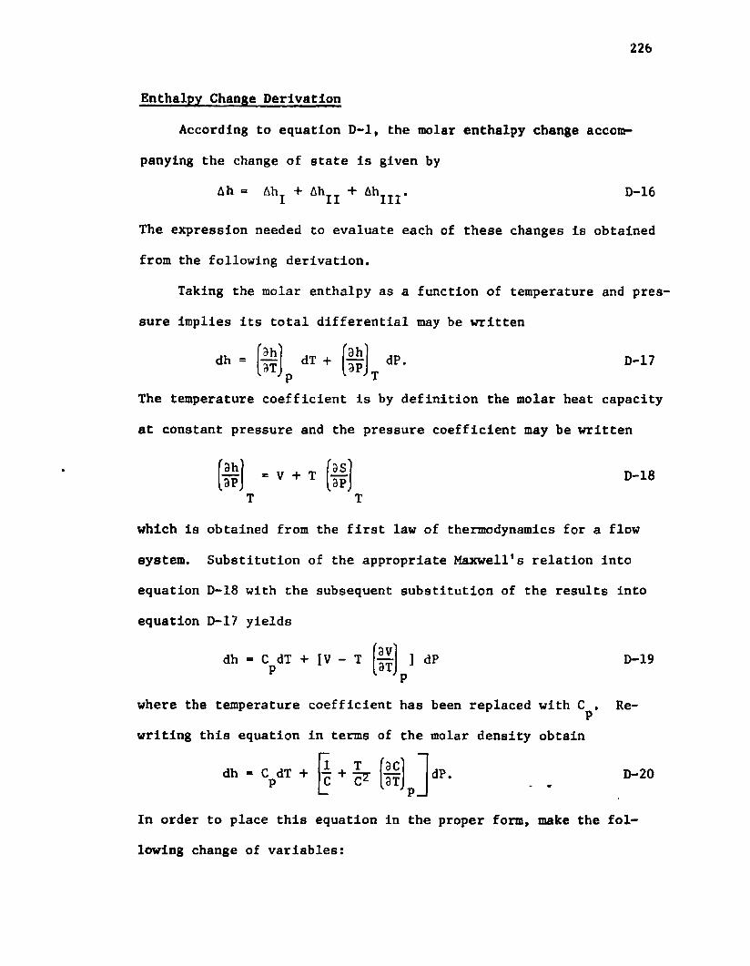
226

Enthalpy Change Derivation

According to equation D-l, the molar enthalpy change accom

panying the change of state Is given by

Ah - Ahj. + &h1T + Ahm - D-16

The expression needed to evaluate each of these changes is obtained

from the following derivation.

Taking the molar enthalpy as a function of temperature and pres

sure Implies its total differential may be written

dh = 3hST dT + 9h

apdP. D-17

The temperature coefficient is by definition the molar heat capacity

at constant pressure and the pressure coefficient may be written

ahap - v + x , 4§ D-18

T T

which is obtained from the first law of thermodynamics for a flow

system. Substitution of the appropriate Maxwell's relation into

equation D-18 with the subsequent substitution of the results into

equation D-17 yields

avdh = C dT + [V - T P 3T ] dP D-19

where the temperature coefficient has been replaced with C^. Re

writing this equation in terms of the molar density obtain

dP.dh = C dT + PI T T + ~FZ

PJD-20

In order to place this equation in the proper form, make the fol

lowing change of variables:

227

and

^ = d(P/C) + £ dC

3C9T dP Hi*

D-21

D-22

Equation D-22 is obtained according to the following:

P * P(T,C)

implying the total differential of P is

dPS i c " +

Vp]9CJ, dC

which implies at constant pressure

3C3T

'ap) fac 9T J [9P,

C T

from which equation D-22 is obtained.

Substitution of equations D-21 and D-22 into equation D-20

yields

Pdh = C dT + d(P/C) +P t. dC D-23

which is the desired equation in differential form for calculating

the molar enthalpy change. Application of this equation to the

reversible path yields

Ahf o

[d(P/c>] +s. [" Ml dC

C7

C dT + P'B[d(P/C)j

B

Substitution of equations D-7, D-8 and D-9 into this equation yields

after integration

Ah - tCphjCTg) + Cgh2 (T0) + Cgh3(Tg) + h^dg.Cg)2 5 i u

- |CAh < V + CAh^(TA> + CAh3(TA> + h-(TA ’CA » 1777?ft9

+ hid<TB) ' hld(TA) D-25

where the indicated functions have been defined for convenience and

are given by

hi (T) - B RT - 2A - 4C /T2 + 5D /T3-6E /T1* D-26o o o o oh2 (T) - bRT - 1.5a - 26/T D-27

h 3(T) - 0.2a(6a + 76/T) D-28

M T»C) = [3— (3 + 0.5YC2- y V ) e x p ( - Y C 2)] D-29

811(1 * * * *hid(T) “ a T + (b /2)T2 + (c /3)T3 + (d / U ) 1 k . D-30

Internal Energy Change Derivation

The equation needed to calculate the change in the molar inter

nal energy associated with the change in state is obtained from

equation D-23 in the following manner. By definition,the molar

enthalpy is given by

h - E + P/C

from which

dE - dh - d(P/C). D-31

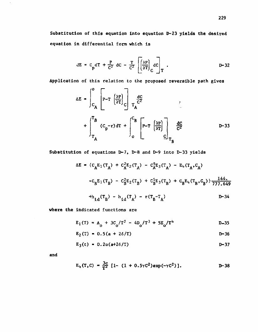
229

Substitution of this equation Into equation D-23 yields the desired

equation In differential form which is

ap3T dC D-3 2

Application of this relation to the proposed reversible path gives(O

' ' dCAE P-T ap3T

fTB CB lP*\(C -r)dT + P P-T (,—)Tj

Jt a Jo C

dCC* D-33

B

Substitution of equations D-7, D-8 and D-9 into D-33 yields

AE « (CaEj(Ta) + C2E2 (TA) - C|E3(TA) - E ^ T ^ )

-cbe,(tb> - C§E2(Tb) f c|e3(tb) + cBE„(TB ,cB))-j?i ^

D-3 4d a

where the Indicated functions are

+hid(V - hid(V - r(W

and

Ei (T) = A + 3C /T2 - 4D /T3 + 5E /T1* o o o oE2 (T) = 0.5(a + 26/T)

E3(t) * 0.2a(a+26/T)

E4 (T,C) = [1- (1 + 0.5yC2)exp(-YC2)],

D-35

D-36

D-3 7

D-38

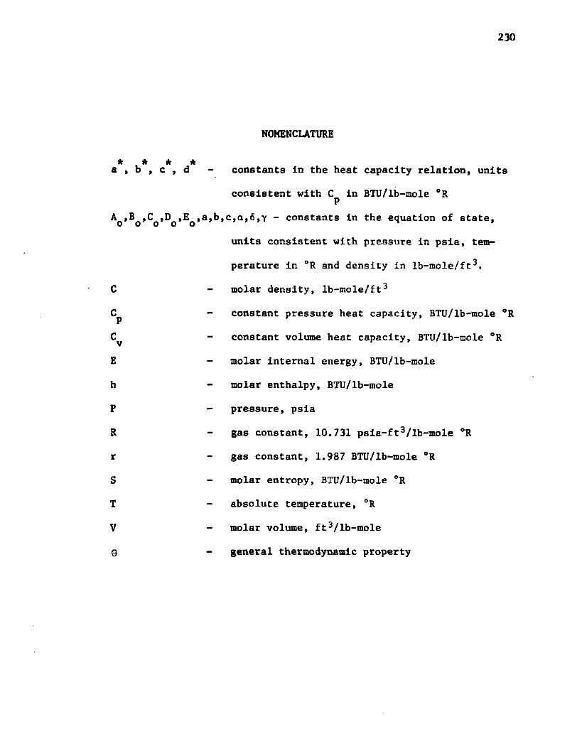
NOMENCLATURE

constants in the heat capacity relation, units

consistent with C in BTU/lb-mole °R P,c,a,6 ,y - constants in the equation of state,

units consistent with pressure in psia, tem

perature in °R and density in lb-mole/ft3.

molar density, lb-mole/ft3

constant pressure heat capacity, BTU/lb-mole °R

constant volume heat capacity, BTU/lb-mole °R

molar internal energy, BTU/lb-mole

molar enthalpy, BTU/lb-mole

pressure, psia

gas constant, 10.731 psia-ft3/lb-mole °R

gas constant, 1.987 BTU/lb-mole °R

molar entropy, BTU/lb-mole °R

absolute temperature, °R

molar volume, ft3/lb-mole

general thermodynamic property

APPENDIX E

CSMP COMPUTER PROGRAM OF THE VSRGM

AND THE VSIGM

INITIALNOSORT

* WRT THE EQUATION OF STATEO* C(1)=0O* C(2)=A0* C(3)=CO* CC4)=DO* C (5)=EO* C(6)=B* C<7)=A* C(8)=0ELTA* C (9 )= ALPHA* C(IO»=C* C (1 I)=GAMMA •/ DIMENSION CPP(♦ ) .CPEC4).CPBC4).CP(5>.CC11).CPRCiI).CEC11).CB(11)/ OATA CPP»CPE .CPB.CPf5)/— I.008568.4.06388E-02.-!•1694E-05.1.316498E✓ *-09,I.292e5.2.363078E-02.-5.114167E-06.3.569067E-10.-5.854331E-OI,/ *5,199243E-02.-1.496386E—05,I.67064 IE-09.1.98717// OATA CPR/.964762,18634.7,79617E.E04.453708.E06.2S6053.E08./ *5.46248.40 066.4.150520.E02.2.01402.274461.EO5,4.56182// OATA CB/1.56588.32544.7.137436.E05•333159.E06.230902.E07./ *9.14066.71181.8•364238.E02.4.0 C985.700044.E05.7.54122// OATA CE/.826059,13439.3.295195.E04.257477.E06.146819.E08./ *3•11206.22404.5.702189... 9 09681.681826.E04.2.99656/FIXEO I.J.IJ

FO=FR*FN YP-1.-YE-YB 00191 = 1 .4

19 CPC I»=YP*CPPCII+YE4CPEC11+YB4CPBCI>m = y p *m p +y e *m e *y b *m b

IFCIJ«EQ.0)G0 TO 7170 RHOI=PI*M/CR*TI)GO TO 8571 P0W=l./3.C C 1>=YP*CPRC 1)+YB*CBC1>*YE*CEC 1 )CC11l=CYP*SQRTCCPRCll>)4VB*SQRTCCBC11))*YE«SQRTCCE<11)>)**2

232

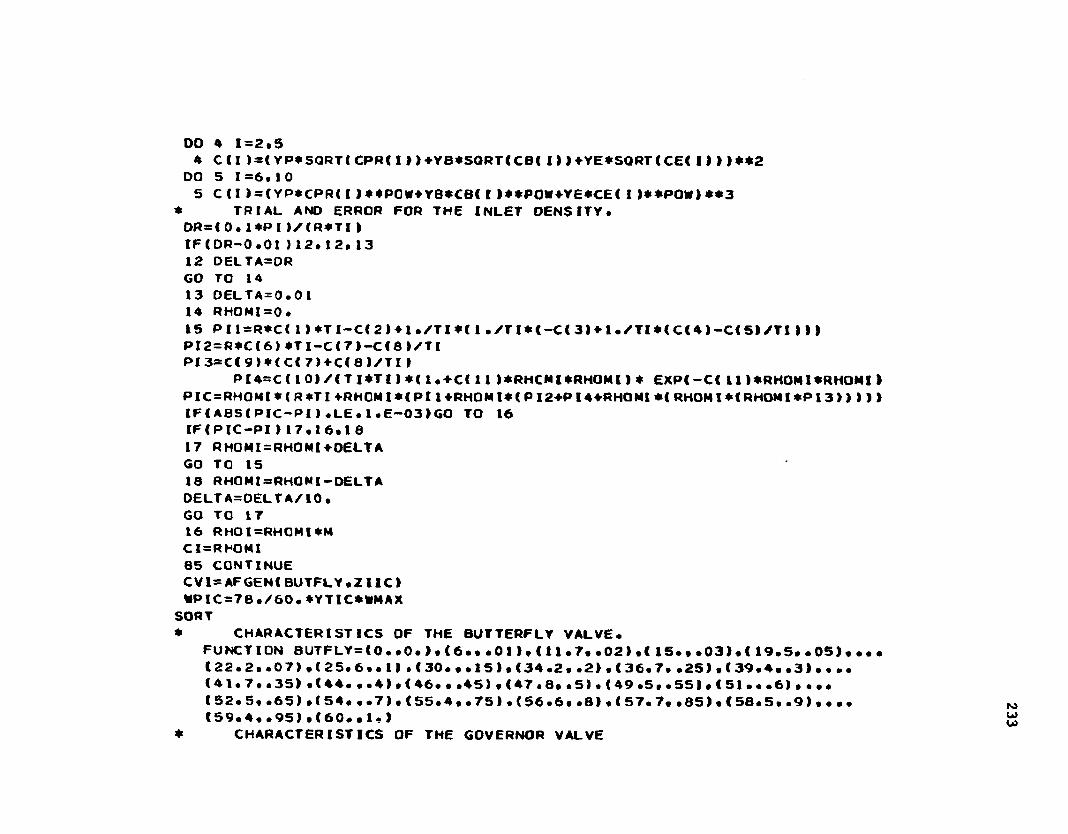
00 4 1=2.54 C(I)=(YP*S0RT(CPRCI))+YB*SQRT(CB)+YE*SQRTCCECI)))**2

OO 5 1=6.105 C Cl) = CYP*CPRCI)**POW*YB4CBCI)**POW*YE*CEC I)**P0W>**3

4 TRIAL ANO ERROR FOR THE INLET DENSITY.DR=C 0.1*PI1/CR4TI)IFCDR-O.Ol)12.12.1312 DEL TA=DR GO TO 1413 OELTA=0.0114 RHOMI=0.15 PI 1=R*CC1)*TI~CC2)*l./TI*C1./TI*C-CC3)*I./TI*CCC4)-CC51/TI»1) PI2=R*CC6)4TI-CC7I-CC81/TIPI3=CC 91*C CC71+CC 8 )/TI 1

PI4=C(10)/(TI*TI)*Cl.*CCU)4RHCNI4RHOMII* EXPC-CCI1)*RHOMl*RHOMII PIC=RH0NI*{R*TI+RHCMI*CPl1*RHOM I*CPI2*PI4+RHOMI*CRHOMI*CRHOMI*PI 3))))> IFCABSCPIC —PI 1.LE•1•E—03 >GO TO 16 IFCPIC-PI117.16.1817 RHGMI=RHOMI+OELTA GO TG 1518 RHGMIs RHONI-DELTA OELT A=OELT A/10•GO TO 1716 RHOI=RHGMI*M CI=RHOMI85 CONTINUECV1 = AFGENC BUTFLY.ZIIC1 *PIC=78./60.*YTIC*»MAX

SORT* CHARACTERISTICS OF THE BUTTERFLY VALVE.

FUNCTION BUTFLY=CO•*0.)«(6.«.01).<11.7..02>.C15...03).C19.5..05).... (22.2..07).C25.6..1).C30..•15).(34.2..21.C36.7..25)•C39.4..3)••••C41.7..35).(44.•.4)•<46.•.45)*C47.8..5).C49.5..55).C51.«.6).... 152.5..65).C54.•.7),(55.4..75).(56.6..8).(57.7..85).(58.5..9)..•• (59.4..95).C60..1«)

* CHARACTERISTICS OF THE GOVERNOR VALVE

233

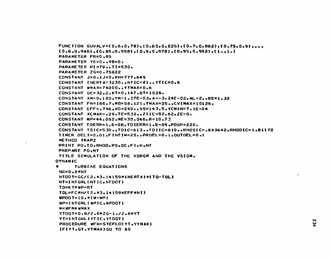
F U N C T I O N G U V A L V = (0 . 6 . 0 . 7 8 ) . ( 0 . 6 S . 0 • 8 2 5 ) • ( 0 . 7 , 0 . 8 6 2 ) . ( 0 . 7 5 , 0 . 9 ) , ( 0 . 8 . 0 . 9 4 6 ) « < 0 . 8 5 , 0 . 9 5 8 ) . < 0 . 9 . 0 . 9 7 8 ) . < 0 . 9 5 . 0 . 9 9 2 ) . P A R A M E T E R F R = 0 .85 P A R A M E T E R Y E = 0 . . V 6 = 0 .P A R A M E T E R P I = 7 9 • . T 1=530.P A R A M E T E R Z G = 0 . 7 5 6 2 2C O N S T A N T J=0, I J = 0 .K H = 7 7 7 .649C O N S T A N T INERT A = 3 2 3 0 . * NTIC = 8 1 . . V T I C = 0 . 6C O N S T A N T MM AX= 7 4 0 0 0 . • V T M A X = 0 .6C O N S T A N T GC= 3 2 • 2 • K T = 0 .147, B T = 1028.C O N S T A N T XM= 0 . 185.YM=I .0 7 E - 0 3 * A = - 3 •2 4 E - 0 2 .AL = 2 . •8 E = I •32 C O N S T A N T F N = 1 8 8 . 7 « M B = 5 8 . 1 2 1 • T M A X = 2 5 . * C V I M A X = 10126•C O N S T A N T E F F =•7 4 6.V D = 2 4 0•.V S = 1 4 3 . 5.Y C M I N = 7 . IE-0 4 C O N S T A N T X C M A X = • 2 9 . T E = 5 3 0 •.ZI IC = 5 2 • 6 2 . Z E = 0 .C O N S T A N T M P = 4 4 . 0 6 2 . M E = 3 0 , 0 4 6 . R = 10.7 3 C O N S T A N T T D E R R = 1 .E - 0 6 . T D I E R R = 1.E - 0 5 . P D S P = 2 2 0 .C O N S T A N T T S I C = 5 3 0 • . T D I C = 6 1 3 . • T D I I C = 6 10•. R H O S I C = • 6 4 3 6 4 2 . R H O O I C = I T I M E R O E L T = 0 . 0 1 . F I N T I M = 2 5 . .P R D E L = 0 • l , 0 U T D E L = 0 . 1 M E T H C O T R A P ZP R I N T P D . T D . R H O O . P S . O C . F I . H . N T P R E P A R E P D . N TT I T L E S I M U L A T I O N OF T H E V S R G M A N D T H E V S I G M .

O Y N A M I C* T U R B I N E E Q U A T I O N SN G = 0 .2*N TN T O O T = G C / < 2 . * 3 . 1 4 1 5 9 4 1NERT A )*(T Q— T O L )N T = I N T G R L (NT I C . N T D O T )T Q = K T * M P - 8 TT Q L = F C * H / ( 2 . * 3 . 1 4 1 5 9 * E F F * N T >W P D O T = 1 0 . * ( M - M P )M P = I N T G R L ( M P I C . M P D O T )M = M F R « M M A XY T D O T = 0 • 8 / 2 • 6 * Z G — 1«/ 2 .6 * Y T YT— I N T G R L C Y T I C . Y T O O T )P R O C E O U R E M F R = S T E F L O < Y T . Y T M A X )I F <Y T . G T •Y T M A X )GO T O 60

•81172

234

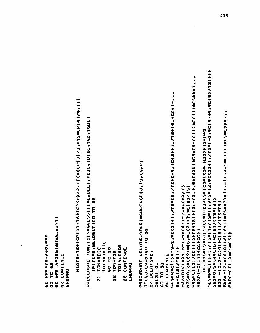
=AFG

EN(G

UVAL

V.YT

)

235

to

UJ3 z 00

oc a z oIL (J IL O OE» H * U (LQi □ O N Zto o *0 »0 UJ

*s

ao«</>•10S00toay00»to

CM\* *CMway«10k4

au*<0I-II(0

ooi-•oC?»OoKJ00a»-JU ioUl CM X CM

oHOo0mH_iUio•UiV3

(0<0Ul3OIIz

*zaF-UJa3aUJyaaa

y •* o o Ui U l « - O CM O O 3X O H y zM K II O KH II Z t- IIW z « zu. o a o o*-1 H K o

CMCMCM

sz« z o o o a c- y a a

o zCM UJ

• * A• * in• to1 u y

0m # »0 0m •

00 ♦ •u 00 ♦ •» 00 0m •• u ♦ #to * 00

4 4 0m y CO• 00 to« yCO 00 ♦ • »1- 00 r m CON y ♦ I y• 1 0 0 #•* co 00 * 0m

♦ y 00 to 00

a * 00 ►-10 CO tos 00

4 4 y 10 • y0m u * X 00 #a • 0m ♦ 10• • 00 « A •<0 ♦ 00 to10 4u t 00 y •• w y 00 y 00CO * • ♦ » 00

♦ - 10 CO CO• |• ►» CO00 • y CM •\ KCO♦ 00 44 00

00 • V *0 • * * 00

00 4* 4 4 \ >0 COco *o w CO44V y »- 00

z * wco 1 ♦ V *m r>Ui CO y 00 • CO• to(0*y K • y r> CM•4 1"H«3 V • • 00 X 00 • * COCO • CM• * 00 • toCOKH 00 1I* * CO1- K*«• 4 44 ♦ CO CO1- w00 00

CO N0m K y VNs 00

.J CM 44 N* ♦ • 00

Ui <0 44 u 00 CO00 CO COM00

o CD U • V H «■* W00 00y• * 10» * toX* y V VCOO • • • 00 y wCO+ y sHC- CM 00 <C 00 * * t0 « aX 1 100 00 COCO\ <0A 0 0

J o CO0m (0* 00 u y • 00 O' oUi o • 1- 0m ►»44 u # ii y 00 •4a o UJ# 0m * a w4 4 co•f * y

o h 3 A to44 N 44 i- 00 a * yUi • CO z 4* H u 00 44 X 00 CM*a; o K • CO00 00 Sw * O00 ml V * • •3 Ui X o CO u u CM4* y UJ y COo CMp • J II z * in * • 4 4 i a « • 00 00

UJ -> UJ mm o u a <00 a o y a o I 1y Mo CO u ii y H II if a ii II II IIo 00 -J to* 10toCOX 10toCOCOa U. NUi o <0 00 • CM•o•* UJ V* CM10♦a 00 COo o CO X toX XX • COCOCOto

(0U#toUi*

yI*0axUi

DELS

I =

(CS*(S

ISft

CS*(

S2S+

CS*(

CS*C

CS*S3S)))J*

S4S1

*I4

4*/7

77.6

49

68 CO

NTIN

UE

ENDP

flO

236

0%

0k 00

• 00

fO • • •

s m n • Ov •

N s • •

to 00 00 • <000 ♦ ♦ ♦ • toa 00 00 00 N 00

u • a a # N u

« UJ u u 00 N f t

V) a * * u S •

b D 00 (VI * • • (VIft k o O • * 04

• < b b • * 00

CM a ft ft i * to# f t

N UJ • • 00 00 f t (VJ

00 a (VI (VJ • o 00 a

n z N \ (VJ u 04 b00 UJ 00 00 00 O * a \a ►- w 00 00 b o b •

u # «0« * \ u * 04

w UJ a k0 a 00 • f t tn f t

f t V u a u a «0 *0 ♦

in a 00 y v 04 * n►- < * * * # 04 00 00

♦ X 00 00 "1 (VI (VI m 00 * u00 u o o o o 00 u 00 *

(VI in >0 b b b u f t 04 •

00 04 • f t f t * ♦ « m Qa o a 00 00 00 • • K i

u • (VJ r> (VJ n (VJ ♦ n 00

w u a 00 w V 00 00 • in f t

* to# 04 u a a a a * 04 * (VJ«0 U) a 0 u u 0 V (VJ 00 o o

J o 00 00 00 00 00 o 1 u »-

f t U i a X * * * • b • 00 s0*. o b a 00 to# (VJ (VJ s 00 04 f t •

00 V) I z • o a O a • 00 00 o 04

00 r- 0« UJ a b b b to4 tvj f t V 00

o 00 tn in a f t ♦ ♦ ♦ to# O ^0 00 00 f t

a u u 00 Ul 00 #to 0k 00 # H (VJ n f t (VJ

X o V 00 tot (VJ (VJ (VI (VJ * Q • o oa J a UJ o 00 o 00 a 00 a IVJ H u b• < u X »- 00 J- a (VJ a b Q » (VJ f t s

IT to# • o 00 u o to# u N b (VJ o 04 0

O • o z b 19 ♦ b o ♦ • 00 O b a *4

UJ 00 o a M IL O •# a IL o (VJ •0 s H f t H 00• A J o o O J o 00 O J O 00 00 w • (VI f t

•0 in < IL H tn IL a 00 O < a 00 00 O u 00 00 f t X t -

V u in a z (VI a 00 #to tn 19 a. 00 00 »- + <0 u o a V

X i w a U l N _» UJ m in N UJ in in V 00 00 00 u i •

a a a b < 00 00 00 M 00 J 00 00 00 • « u V « f t m *0

w «4 u UJ 00 O UJ o a a X tn < o a a 00 00 00 * A Q 04 in 00

h* *0 ♦ o b o b u u a H Ui b u V 00 u 00 00 U o j f t00 a tn a II 00 • i i i J s • i i 00 00 * <?> o ft 1- UJ (VI

Z u H z 00 a z 00 00 to# UJ Z 00 *4 00 a 00 04 O 04 o o00 o < o o UJ 00 00 *0 o o UJ M to# 00 00 00 u 00 u in f t K

J n to# 00 UJ X a 00 00 H 1 UJ r a w 00 (J (VJ * * u f t 00 to# s

II tn in j o D b b a 0. O 00 D b b a a * O in (VJ * 00 f t O •

z a z ►- ii < UJ • Z 00 u u to# o Z 00 u u a b • • • to# a J - •M

o V a k0 to# a a 00 a -1 00 00 in b to 04 a J 00 to# 00 V o o (U to# u o 1V> X o 04 X a D UJ b o a II II H II 00 N b a a II II 1 i 00 w to# 00 44 II

□ a □ tn a b O • Z IL z 0« a to# 00 O Z IL z 00 a II in ii II II u II in a .

X X UJ -> a 00 Q •>* V) Q b O o 00 O 00 00 00 04 04 04 T r> ii 04

a a u 00 u II J - o b b II b o II ►- o o u a a a w in tn Q

ii i i o 00 «0 O b J IL 00 (VJ o L* H * k b a J J bV) o a IL i*j a 00 Q UJ O o O (VJ a 00 O >0 • (VI n * X UJ UJ to*

u u a 00 h> H in in a IL b t9 n - b in in in ♦ tn in in UJ o o tn* * *

-20.*C

(5)/

TD2)

) ))

>S2TDIP=C< 8>

/T02

**3

S3TDI P=

—(0.4*CC 9

)*C(

8}}/

TD2*

*3S4TD IP

=-(6

.*C(

10)

)/(C

< 11

)*TC

2M4)

*(1.

-(1.

+ .5

*C(

11}

*CO*

CO)*

. • •

237

*a44

Qy4W♦

aMoynin#oy

ou44*a

y♦a

oyCMW44* aQ V)y a y♦ •4 UJa o oa 44 y Vy o O V)# y V) yu + UJy 10 o- O# w 4 14k # o PO•4 o • Q

wm y N y44 s IIy n N CMi a V aw a) • ya _i * 11X UJ □UJ o -4 U.

*44

oy♦•tnx n44aywOy♦• ao j a v •0m 4k

CM O -> ya • u o 44 y

* •o «y 44♦ y« M "* 0.O a a

y y

M QO H y XUJ M3 oZ y44 Qt\JK kk

O z O Xy u aII y a►H ao 4 zy N UJ

•.•4k444y*•in*•4oys•0*♦4kmwy••♦i«4«k4oy 44\ o 44• y M>4 N o44 4ky* ® s44 k441o y COy * k4s • y* CM»*4 1 •* 4kNy ♦w 444kk4 y yy • V« in y• • *cm «4 •i 1mm 44k4o — o #y — y Ml* 4k« O'4k 44* 44— o iu •* o <0 yo n 3 w h — *• w z y n y cmo q * .UKffhainito

* - Q * - y o * o o m» y • »- yU . O O O - O M r o - o o o i i x r

♦**oy•

y 44

* a4k y.4 ♦ (J)4* X y

44 ♦ oy 4k 44

1 4k Xo 4k •y 4k 44

* 44 oq P ya y o• in 444 * X X44 # 4444 o ♦k4 y 0»y 44• # «m O .• y N♦ 44 N• * y

ro O \0 0 y 4k

i ♦ •• 44 ♦tn o ♦k4 y 44

• CM *4k X 4k44 44 ina # y

y o X« y Jk4 ♦ UJo 44 ay 4k a »# 4k y M

4k a •4 a44 y X y•4# 44 X44 a * jy y o ak * • y 44\ 0m n 444k4444UJ IIo 44o 3 4444k4 y Z X44y X44 Jy * j y 111n 44a z □ o44 a o ao X y ay UJ o

* * zX 4k O' UJ

UJz4k►»•z•X<zyx•z*4zy>z.UJnj<.<►.zx

a</>aa

zy

u. z «ku. ■4yUJ y < os z « 444 44* mX u. 4kO'ml . y inUJ y Z .o z o * COII s • mUJX X UJ o 4koml J a <0z aUJ UJ 3 44> 3o o a 44 1 </>

* UJ \ yX y X >X o <144II a y u.X a y 44

40 F I N T I M s T I M E Q C=0.W R I T E ( 6 * 6 0 0 )

60 0 F O R M A T ! I X . * T H E C O M P R E S S O R H A S E N T E R E D S U R G E SO H A L T T H I S C A S E * * / / )G O TO 46

* O N T H E V E R G E OF S U R G E 3 9 Q C = ( 6 0 . * N T ) * * B E * X M / 6 0 .G O TC 4638 I F ! Y C . G T . Y C M I N > G O T O 41

* U P A G A I N S T T H E S T C N E WALL*42 Q C = ! 6 0 * * N T > * * B E * X C M A X / 6 0 •W R I T E ! 6*620)6 2 0 F O R M A T ! • C C M P R E S S O R AT S T O N E W A L L * )GO TO 4641 X C = X M + S Q R T ! ! Y M - Y O / I - A ) )Q C = ! ! 6 0 . * N T ) * * B E * X C ) / 6 0 .46 C C N T I N U E E N D P R O

P S I = D E L H T S * 1 4 4 . / 7 7 7 . 6 4 9 * H I O T S + O E L H

* T R I A L A N D E R R O R F O R T H E A C T U A L O I S C H A R G E T E M P E R A T U R E *P R O C E O U R E T O = D T E M P ! T O N * T D E R R * P S l * C D * R * I J )I F ! I J . E O . O ) G O TO 76 77 C O N T I N U E

* F O R T H E IOEAL G A S T D I G = I M P L l T O N . T O E R R . F T O I G )H I O T D G = T O I G * !C P ( I )F T O I G M C P ( 2 ) / 2 . + T D I G * ( C P I 3 ) / 3 . F T 0 £ G * C P ! 4 ) / 4 •)))H I D T GP=CPI I ) F T O I G * ! C P I 2 ) + T D I G * ! C P < 3 ) + T O I G * C P I 4)))O H T O I G = H I O T O G — PSI F T D I G = T O I G — O H T O I G / H I O T G P T D = T D I G G O T O 78 76 C O N T I N U E

« F O R T H E R E A L GAST D R s I M P L ! T O N * T O E R R *FOFTOR)

238

239

• o*• *• <oPB •* Nbp Nu s •

PB 77 \ PB • PBPB • PB • PB • PBPB in PB * Q PB PB• w o ♦ CJ a cn

♦ • cj •4 • « z *V a • * • o o NPB o a PB • CJ PB♦ t- cj a w * ♦ inBP s * a » PB z BPa • pb w> z «p ♦ CJ PBu *p m* ♦ a pp PB T in PB* ♦ Z BP PB PB CJ PBa *0 4 V CJ PB 9 * 04Q n u * • t PB 00 <n *7- BP 1 PB pa BP (L CJ CJ PB♦ PB cj BP 00 ♦ a S BP * cn• PB * a 00 PB X O « 00 CJ

**7 A • X z n Ui 7- in m* »S * UJ o BP * 1*7 7- mmr*7p b BP 1 * CJ PB Z S «■* inn a BP n * « • • CJ aBP u * 9 z • • a •a 1 BPa * a • • CD * CJ ♦ BP 77cj a o 77 a BP O BP PB a in*0 a K a o CJ * • CJ « 1*7 X CJ* 7- S o a <J BP z • » a BP UJ BPz ♦ • t- z 77 » a • PB CJ CJ # 77a mm*4 \ o mma t- » •P Bp 1 PB int- 1*7 BP a 7- u \ PB PB Pp • BP in CJ4 • CO\ Bp • z 1*7 BP o * CJ 4• a z BP • mm* ** A o • CJ CJ cn * 9

CMu o u CO • CJ o BP z h* * * + PB 7* in ins K * BP • * CJ » o » a 00 a a S CJ aA * \ • CJ * 4 z Z o 04 z • • * 4CMa • CM77 PB wri z Q * u H 04 o cn pp PB CM

o pp 1 • a mi a K PB z t- • BP K u 40 cn PP cna H 4 PBN o ** N, PB Q BP PB CJ CM • * 7- «B au ♦ A N ♦ 7- u CM • PB K \ Bp 1 X in in \ W wBP PB CM Bp PB * 1 Z M 04 PB PB *4 Q BP 7- PB PB u ** CM*0 u N a a BP cn 00 z \ PB ** CJ * a • V COin 4 inz w> u 77 BP a o * a * □ PB COCJ » o z -» • Bp 7* • CJo a * in U 7- • a i z COBP BP O CJ a 04 pp CJ \ pp 4t- cj • • * # Q CJ a o \ w CJ \ CJ ♦ a 7> BP O' 4 1 PB BP pp4 w CM pp • PB CJ 4 o PB CJ * PB • a z Q a N PB PB (0 * cnPB * 1 1 <0 * z ►- V in « PB PB PB z a V »- CM7» BP PB aPP a cr z bp m» PB a o • • o> o PP a 7- z <j a BP BP CJ cn BPBP o a A o * W •0 7- M CJ CMBP 04 mm•- O' BP a 3 7- CJ CJ 4 7- *a t- 7. A ►- PB u 04 z + * * CJ BP W mt « z 7- cn 1 1 0 cj PB 77 * a S0 CM BP • • in * N z i UJ a • * UJ * * CJ BP in UJa BP i- BP <7 o in a ►- u + o ** CM • o N o z 3 o Z 3 A PB BP \ 7- 3Q a u \ u CM ■4 mu z » PB * w BP + u N 7- Q Z UJ • • Z >0 * PB * ZH u « PB * • bp 4 w j z •* z 1 1 • BP V Z 7- pp z a cn mmpp V BP o z mm

U ii a in a O CJ • II o II Bp II II II n II • a II 7- 3 UJ CJ «0 7- U CJ O' pp BP Hoc a n v ii II II n z II a CJ a a a BP a ♦ ii Z z Z O O • ll Z * * Bp BP 77 z oCJ z a U a: a a 00 a z a # a a z 1 z 9 a u a a z UJ 3 cn a a z Z u CJ cn a z

c a * o o a I 7- o a • a o a • a 04 z ►- 7" CJ a CJ kP a 7- CJ II II II II u CJ ao »■• h • 7p t- • z h> ►- in H »- 7- 1*7 7- # a IL II o O w pp CM 1*7 9 ii o

BP mm<0 cm n * n J z 04 04 CM 1*7 < 40 z a a o z z IL o o 0* in in in in in pp zz z X 1 z z z 00 Q o z 1 z Z I a O X 7» N UJ a <0 co a a a a a COUJ

P R O C E D U R E P D = 0 1 S C P C I J *TD , C D , R )I F ( I J . E Q . O ) G O T O 62 83 P O = C O * R * T D G O TO 84 82 C O N T I N U EPDt=R*C(I)*TO-C<2)+l,/TD*( 1 ,/TD*(~C<3) + l «/T0*<C<4 )-C< 51/TOW) PD2=R*C<6> *T0-C(7)-CC8)/TD PD3=C(9)*(C(7WC(8 )/TD>P D 4 = C ( 1 0 ) / ( T D * T D ) 1 •*€{11 )* C O * C D >*E X P (- C (1 I) * C D * C D )P D = C O * (R 4 T D + C D * ( P D I * C D * C P D 2 + P D 4 + C O « < C D * C P D 3 * C D ) )) Me4 C O N T I N U EE N D P R O

T G D I = D E L A Y ( 1 * D E LT»TDI )T G D = D E L A Y ! t . D E L T . T D )

P R O C E O U R E F E = B Y P A S S ! Z E , P O * P S « M , T O )P l E = P D - 0 . I * P C * * 0 . 7 X 2 = P 1 E - P SI F ! X 2 , L E , 0 . ) GO T O 9

11 X 3 = 0 , 5 3 * P 1 E — PS I F ( X 3 > 8 . 7 . 7

* C R I T I C A L F L O W7 F E = 1 . 3 7 4 7 / 0 , 6 * P 1E * E X P ( 4 . 6 * Z E >* S Q R T ( M / T E )

G O TO 10* S U B C R I T I C A L F L O W

8 R H O E * ! ! P S * P I E ) * M » / ( 2 , * 1 0 . 7 31*TE)F E = 8 . 1 7 9 5 / 0 , 8 * E X P { 4 . 6 * 2 E )4 S O R T (R H O E 4 X 2 )G O T O 10

9 F E — 0,10 C O N T I N U E

F E = F E / 6 0 ,E N O P R O

P R O C E O U R E F I = F L 0 W I N ( C V I , P I , P S , R H O I ,R F O S . C V I M A X )

240

D E L P = P I - P S I F ( D E L P I 2 . 2.11 R H C = ( R H 0 I + R H 0 S > / 2 .Fist .0S*CVIMAX*CVl*SQRTCRHO*DELP)/60.G O TO 32 F I =0 .3 C O N T I N U E

ENDPRC

F S = F I + F ER S D O T = ( F S - R H 0 S * Q C 1 / V S R H O S = I N T G R L I R H O S I C . R S D O T )ROOOT =(RHOS*OC-FE-FO>XVO RHOO1=INTGRL(RHOOIC•ROOOTI

TSOOT=CFI*CTI-TS»+Fe*(TE-TS>)/( RHOS*VS> T S=INTGRLITSIC*TSOOT)FC=RHOS*QC

T E R M I N A L J= J+ I

I F ( J . E Q . 3 ) F R = F R + 0 . 0 5 I F I J . L T . 6 1 G 0 T O 102 IF < IJ) 1 0 1 * 1 0 1 . 1 0 0 102 F R = F R + 0 . 0 5

G O TO 108 101 2 G = 0 .69 107 J = 0

F R = 0 .85I J=lD O 109 1=1.11 109 Cl I 1=0.Y T I C = 0 . 5 5 Y T M A X = 0 . 6 F N = 1 7 0 • 3 C V I M A X = 9 6 2 9 . 7 E F F = 0 .846

T D I C - 5 9 1■T D I I C = 6 0 0 • R H O S I C — 0 * 5 8 1 4 1 4 R H O D I C - 1 * 5 2 9 4 5 108 F I N T I M = 2 5 . C A L L R E R U N 100 C O N T I N U E E N D

S T O P E N D J O B

ro

K>

APPENDIX F

COMPUTER PROGRAM FOR CORRELATING THE VARIABLE SPEED PERFORMANCE CURVES

D I M E N S I O N PI 2 ) .SC 2)C O M M O N N P T S C 1 0 ) . S P E E D I 10 ) • HI 50 • 10 ) • 0 1 5 0 . 1 0 ) .1 N C U R • T I T L E ( 1 5 ) . OATEI 2)O A T A S / 1 . . 1 . /IER=0RE ADI 5. 1 0 3 ) D A T E

103 F O R M A T ! 2 A 4 )R E A D ! S •10 0) T I T L E . N C U R

100 F O R M A T ! 1 5 A 4 . 12)D O l 1 = 1 , N C U RR EAOI 5 . 1 0 1) N P T S I 1 ) .SPEED! I ) •

101 F O R M A T ! I 2 . 6 X . F 1 0 . 0 ) i N P T = N P T S ! I )R E A D ! 5 . 1 0 2 ) < H ! J . I ) . 0 ! J . I ) , J =1.NPT)

102 F O R M A T I 0 F 10.0)D G 6 J = 2 » N P TIF(H( J . I l . L E . H ! J-l. D . A N D . Q I J. D . G T . Q ! J-l, I)) G O T O 6

7 M R I T E 16.605) I .H I J . I ) . 0 ! J , I >6 0 5 F O R M A T ! * INPUT E R R O R IN C U R V E N U M B E R * . 1 3 /6 051 • H E A O = • , I P E 12.5.* A C F M = * ,E 1 2 . 5 )

I E R = I E R 4 1 6 C O N T I N U E

I F ! I E R . G T .0) S T O P O C 1 J = 1 . N P T H! J . I ) = HIJ »I ) ♦ 1 .E03

1 Q ( J , I ) = Q | J . I ) * 1 . E 0 3 D 0 2 K = 1.4C A L L S W I T C H ( 4 . J T E S T )I F ! J T E S T - 2 )8 . 9 . 9

9 K L = K - 1 J L = 3 - K L P ! 1 )=KL P ! 2 ) = J LP R I N T 6 0 0 . T I T L E . D A T E . P

6 0 0 F O R M A T ! 1 H I • 1 S A 4 « S X .•D A T E * . 2 A 4 /6 0 0 1 • S T A R T I N G P O I N T ••••• A= • . F 3 •1,2 X . •B = * . F 3 . 1 / / >

C A L L P A T E R N ! 2 * P * S « 4 * 1 * C )C A L L P R O C ! P * — 1*1

2 C O N T I N U Ea P A U S E * SET S E N S E S W I T C H I H I G H A N D I N P U T P ( 1) A N D P C 2 I * 2F6* 0 • 5 C A L L S W I T C H ! I . I T E S T )

IF C I T E S T — 2) 3 * 4 * 43 R E A D ! 2• 2 0 0 ) P

200 F O R M A T ! 2 F 6 . 0 )I F ( P G O T O 4 P R I N T 6 0 0 • T ! T L E * D A T E * P C A L L P R O C ! P * — I• I G O TO 5

4 S T O P E N D

245

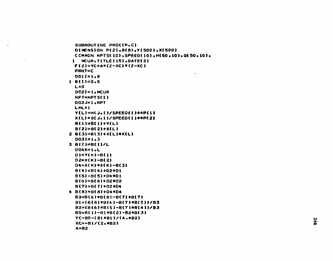
S U B R O U T I N E P R O C ( P * C )D I M E N S I O N P ( 2 > . B ( 8 ) , Y ( 5 0 0 » . X ( 5 0 0 I C C M M O N NPTSI 10) «SPEED! 10 ) • H CSO • 10)• Q< 50 • 10) •

1 N C U R * T I T L E 1 1 5 ) «DATE< 2) F I Z ) = Y C * A * C Z - X C ) * I Z - X C >P R N T * C D 0 1 1 = 1 * 8

1 B CI)=0«0 L = 0D 0 2 I ® 1 • N C U R N P T = N P T S ( I )D 0 2 J * 1 • NPT L = L * lY ( L ) = H ( J . I ) / S P E E O B ( 2 ) = B ( 2 ) * X C L )

2 8 C 3 ) = B ( 3 ) + X ( L ) * X C L )0 0 3 Is 1*3

3 B ( I ) = 6C I l/L D 0 4 K = 1 . LD1 = YC K ) - B ( 1)D 2 = X C K ) - B C 2)D4=X< K)*XC K ) — B | 3)B ( 4 ) = B ( 4 ) * D 2 * D 1 8 ( 5 ) = B ( 5 ) *0 4 4 0 1 B(6 ) = B< 6) + 0 2 * 0 2 B < 7 ) s B < 7 1 * 0 2 * 0 4

4 B ( 8 ) s 8 ( S ) * 0 4 * 0 4 B 3 = B ( 6 I*B ( 81 — B I 7 ) * B I 7)Bl = (BI 8 ) * B (4 ) — B I 7 ) * B ( 5 ) ) / B 3 B 2 = ( B ( 6 I * B ( 5 ) - B ( 7 > * B < 4 ) ) / B 3 B O = B ( 1)— B l * 8 1 2 ) - B 2 * 8 C 3)Y C = B 0 - ( B 1 * B 1 ) / ( 4 . * B 2 >X C = - B 1 / ( 2 « * B 2 )A = B 2

M=0C=0.00 0 6 1 = I* N C U R N P T = N P T S ( [)D 0 6 J = 1•NPT M=M-f 1H P = F ( X ( M ) >* S P E E D C I )* * P ( I >D I F F = H < J,I I — HP

6 C = C * D I F F * D I F FI F (P R N T , G E ,0•) R E T U R N S = S Q R T ( C / ( M - 5 > >M=0P R I N T 6 0 0 , Y C . X C . A . C . S . P

6 0 0 F O R M A T * /✓✓.' TH E E Q U A T I O N IS V * Y C 4 C * ( X - X C ) **2 *6 0 0 1 //• Y H E R E * / / 2 0 X . * V C = • , 1 P E 1 2 . 5 / / 2 0 X ,6 0 0 2 • XC= • . E 1 2 . 5 / / 2 0 X , * C = • , E 1 2 . 5 / / / / 12X,6 0 0 3 ' S T A T I S T I C S * / / * S U M E R R O R S O U A R E O » • • E 1 2 . 5 / /6 0 0 4 • S T A N D A R D E R R O R OF F I T = * • E 1 2 , 5 / / / / 12X,6 0 0 5 ' E X P O N E N T S * //• A* • . E 1 2 . 5 . I O X .•0= * , E 1 2 , S )

D 0 7 1 = 1 , N C U RN P T = N P T S C I »P R I N T 6 0 1 • T I T L E , D A T E ,S P E E D ! I )

601 F O R M A T * 1 H 1 . 1 5 A 4 , * 0 A T E * , 2 A 4 / a S P E E D = • , F 6 . 1/6 0 1 1 6 X ,* Q * , 1 3 X , * H * , 1 0 X , * H P R E O I C T E D * ,5 X ,•D I F F * •6 0 1 2 9 X , ' P E R C E N T * )

0 0 7 J = 1,NP TM = M+1H P = F ( X * Ml 1* S P E E 0 • 2 X . 0 P F 9 . 4 )

N R I T E ( 2 , 2 0 0 ) S , P2 0 0 F O R M A T * • STD. E R R . = • • 1 P E 1 2 , 5 , 2 X . •PC 1>= • . 0 P F 8 . 5 . 2 X , * P ( 2 1 = ••

SFB.5)R E T U R N

247

E N T R Y a O U N O S ( P « I G )1 0 = 0I F ( P ( 1) .LT . 0 . C R . P C 2 > . L T . 0 IR E T U R NEND

10=1

248

n ft

n

S U B R O U T I N E P A T E H N I N P . P . S T E P . N P A S S , 1 0 , C O S T )

C G E N E R A L M U L T I V A R I A B L E S E A R C H P R O G R A M T O M I N I M I Z E A C O S T F U N C T I O N C U S I N G P A T T E R N S E A R C H M O O I F I E O TO INCL U D E C O N S T R A I N T S C

C—Cccccccccccccccccccc*»

" D E F I N I T I O N SN F -----N U M B E R O F P A R A M E T E R S T O BE S E A R C H E D (IN T E G E R )P ------P A R A M E T E R S TO BE S E A R C H E D I V E C T O R OF L E N G T H NP)S T F P — I N I T I A L S T E P S I Z E OF E A C H P A R A M E T E R ( V E C T O R O F L E N T H NPI N P A S S — N U M B E R OF P A S S E S T H R O U G H P A T T E R N W I T H THE S T E P S I Z E O F E A C H

P A R A M E T E R R E C U C E D BY A F A C T O R OF 1010 O U T P U T O P T I O N A V A I L A B L E IN S U B R O U T I N E P A T E R N

I 0 = 0 • • • • N O O U T P U T1 0 = 1 . . . .F I N A L A N S W E R O NLY* P R I N T E D 1 0 = 2 . • • . R E S U L T S O F E A C H I T T E R A T ION P R I N T E D 1 0 = 3 * . • . R E S U L T S O F E A C H S T E P P R I N T E D

C O S T — C U R R E N T V A L U E OF T H E C R I T E R I O N F U N C T I O N B E I N G M I N I M I Z E D

B C U N D S I P . I O U T ) S U B R O U T I N E W R I T T E N BY U S E R TO C H E C K FO R B O U N D A R YV I O L A T I O N S F O R A P A R T I C U L A R V A L U E OF T H E V E C T O R P. P R O G R A MS H O U L D BE W R I T T E N S O W H E N A V I O L A T I O N O C C U R S IOUT IS SET E Q U A L T O O N E AND W H E N N O V I O L A T I O N O C C U R S SET E Q U A L TO Z E R O

P R O C ( P . C O S T ) ------- S U B R O U T I N E W R I T T E N BY U S E R TO C A L C U L A T E A V A L U EO F C O S T F O R A P A R T I C U L A R S E T O F P A R A M E T E R S * P.

D I M E N S I O N P ( N P ) * S T E P ( N P )•B I ( 10).B2( 1 0 ) . T( 1 0 ) , S( 10)CC * * * * *N O T E * * * V E C T O R S B 1 * B 2 * T * S N E E O O N L Y BE D I M E N S I O N E D BY A N U M B E R

E Q U A L TO THE N U M B E R O F P A R A M E T E R S . NP.

- S T A R T I N G P O I N T N R D = N P A S S L = 1

P T R N O O O O KPTRNOOOt P T R N 0 0 0 4 P T R N 0 0 0 5 P T R N 0 0 0 6 ►P T R N 0 0 0 7 P T R N 0 0 0 8 P T R N 0 0 0 9 P T R N O O I 0 P T R N O O I 1 PTRNOO12 P T R N O O I 3 P T R N O O 14 P T R N O O I 5 P T R N O O 16 P T R N O O I 7 P T R N O O 18 P T R N 0 0 1 9 P T R N 0 0 2 0 P T R N 0 0 2 I P T R N 0 0 2 2 P T R N 0 0 2 3 P T R N 0 0 2 4 P T R N 0 0 2 S P T R N 0 0 2 6 P T R N 0 0 2 7 ► P T R N 0 0 2 8 P T R N 0 0 2 9 P T R N 0 0 3 0 P T R N 0 0 3 1 P T R N 0 0 3 2 P T R N 0 0 3 3 P T R N 0 0 3 4 P T R N 0 0 3 5 P T R N 0 0 3 6 P T R N 0 0 3 7

sc—

6

C—11

12

20 C --

21

10

I C K = 2 I T T E R s O 0 0 5 1 = 1 , N P B i m - p i i )B 2 C I > = P t I )TCI 1 = P C [)S C I ) = S T E P C I )* 10•- I N I T I A L B O U N D A R Y C H E C K A N D C O S T E V A L U A T I O N C A L L B O U N D S C P . I O U T )IF C I O U T . L E . O )G C T O 10

I F C I O . L E . O ) G O T 0 6 H R I T E C 6 , 1005)MR IT E ( 6 » 1 00 0 > < J , P C J ) • J= 1 • N P )

R E T U R N C 1=0 .C A L L PROCC P , C 1>

I F C I Q , L E • 1 I 6 0 T 0 1 1 MRI T E C 6 , 1 0 0 1 I I T T E R . C 1 M R I T E C 6 , 1 0 0 0 1 C J . P ( J ) . J = 1 , N P )

------ B E G I N N I N G OF P A T T E R N S E A R C H S T R A T E G Y0099 I N R D = 1•N R D 0012 1=1.N P SCI> = S ( I 1/10.

IFC IO.LE. D G O T 0 2 0 N R I T E C 6 . 1003)M R I T E I 6 . 1000 M J . S ( J ) .J = l . N P >

I F A I L = 0 .0 P R E T U R 8 A T I O N A B O U T T

0 0 3 0 1 = 1 , NP I C=0P C I ) = T C I 1 * S C I )IC=IC+1C A L L B O U N D S C P . I O U T 1 I F C I O U T . G T . O )G O T O 23 C A L L P R 0 C C P . C 2 )

L = L + 1

PTRNOO 38 P T R N 0 0 3 9 P T R N 0 0 4 0 P T R N 0 0 4 1 P T R N 0 0 4 2 P T R N 0 0 4 3 P T R N 0 0 4 4 P T R N 0 0 4 5 P T R N 0 0 4 6 P T R N 0 0 4 7 P T R N 0 0 4 8 P T R N 0 0 4 9 P T R N 0 0 5 0 P T R N 0 0 5 1

P T R N 0 0 5 3P T R N 0 0 5 4P T R N 0 0 5 5P T R N 0 0 5 6P T R N 0 0 5 7P T R N 0 0 5 8P T R N 0 0 5 9P T R N 0 0 6 0P T R N 0 0 6 1P T R N 0 0 6 2P T R N 0 0 6 3P T R N 0 0 6 4P T R N 0 0 6 5P T R N 0 0 6 6P T R N 0 0 6 7P T R N 0 0 6 8P T R N 0 0 6 9P T R N 0 0 7 0P T R N 0 0 7 1P T R N 0 0 7 2

250

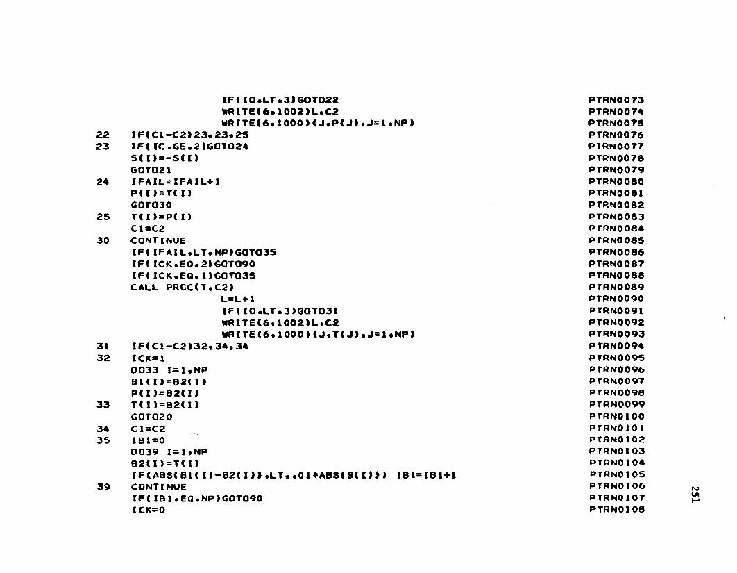
2223

24

25

30

3132

33

3435

39

I F ( I O * L T • 3 1 G O T 0 2 2 W R I T E I 6 . 1 0 0 2 1 L . C 2 W RITE! 6* 1 0 0 0 M J . P ! Jl. J - I * N P >

I F 1 C I —C 2 1 2 3 * 2 3 * 2 5 IF( IC . G E . 2 I G G T 0 2 4 S ! I ) = - S ! I )G 0 T 0 2 1I F A I L — I F A I L + 1 P ( I > = T| I )G 0 T O 3 0 T ! I > = P C I )C 1 = C 2C O N T I N U EI F ( I F A I L * L T • N P I G 0 T 0 3 5 I F ! I C K . E Q . 2 1 G 0 T 0 9 0 I F ! I C K . E Q . 1 1 G 0 T 0 3 5 C A L L P R G C I T . C 2 )

L = L + 1I F ! I O * L T • 3 1G0T031 W R I T E 1 6 * 1 0 0 2 J L » C 2 W R I T E ( 6 , 1 0 0 0 ) ! J * T ! J ) . J = I . N P »

I F ( C 1 — C 2 ) 3 2 » 3 4 * 3 4 I C K = 10 0 3 3 1=1 * N P B 1!I)= B 2 ! I>P ! I ) = B 2 ! I )T ! I )= B 2 ! I )G O T O 2 0 C 1 =C 2 I B 1— 00 0 3 9 1=1* NP B2!I 1= T ! I)I F ! A B S l B 1! I)— B 2 ( I ) ) * L T * * 0 1 * A B S ! S ! 1 1 1 1 181=181 + 1C O N T I N U EI F ! I B 1 • EQ* N P I G O T 0 9 0 I C K = 0

P T R N 0 0 7 3P T R N 0 0 7 4P T R N 0 0 7 5P T R N 0 0 7 6P T R N 0 0 7 7P T R N 0 0 7 BP T R N 0 0 7 9P T R N 0 0 8 0P T R N 0 0 8 1P T R N 0 0 B 2P T R N 0 0 8 3P T R N 0 0 8 4P T R N 0 0 8 5P T R N 0 0 8 6P T R N 0 0 8 7P T R N 0 0 8 8P T R N 0 0 8 9P T R N 0 0 9 0P T R N 0 0 9 1P T R N 0 0 9 2P T R N 0 0 9 3P T R N 0 0 9 4P T R N 0 0 9 SP T R N 0 0 9 6P T R N 0 0 9 7P T R N 0 0 9 8P T R N 0 0 9 9P T R N 0 1 0 0P T R N 0 1 0 1P T R N 0 1 0 2P T R N 0 1 03P T R N O 104P T R N O 105P T R N O 106P T R N O 107P T R N O 108

251

ITTER=ITTER41 PTRNOI09IFCIO.LT.21GQTO40 P T R N O 110MRITEC6.1001) ITTER.C1 P T R N O I 11MR ITEC 6.1000)CJ.TCJ).J=1.NP» PT R N O I 12

c----- -ACCELERATION STEP PTRNOI1340 SJ=l.O PTRNOI14

0045 11=1.11 PTRNOIIS0042 I=1.NP P TRNOI16T (I> = B2CI)+SJ*CB2CI>-B1(1) ) P TRNOI17

42 P( I ) = TC 11 PT R N O I 18SJ=SJ— •1 PTRNOI19CALL BOUNOSIT•IOUT) PTRN0120IFCIOUT.LT.l)GOT046 PTRN0121IFCII.EQ.11)ICK=l P T R N O 122

45 CONTINUE PTRNOI2346 0047 1=1.NP P T R N O 12447 B 1 CI)= B 2 C I ) P T R N O 125

G0T020 P T R N O 12690 0091 1=1.NP P T R N O 12791 TCI )=B2CI> P T R N O 12899 CONTINUE P T RNO129

D0100 1=1.NP P T R N O 130too PCI)=TCI) P T R N O 131

COST=C1 P T R N O 132IF CIO.LE.O)RETURN PTR N O 133MRITEC6.1004)L.C1 PTRNOI34MRITEC6.1000)CJ.PCJ).J=1.NP) P T R N O 135

RETURN PTRNOI361000 FORMAT C10X.5CI7.E13.6)/) P T R N O 1371001 FORMATC//1X14HITTERATI ON NO. • I5/SX.5HC0ST= •E15.6.20X. P T R N O 138

1 10HPARAMETERS) P T R N O 1391002 FORMAT C 10X3HNO..14. 8X5HC0ST=.EI S .6) P T RNO1401003 FORMAT!/IX28HSTEP SIZE FOR EACH PARAMETER ) PTR N O 1411004 FORMAT! 13HANSMERS AFTER •13.2 X •23HFUNCTIONAL EVALUATIONS /✓ P T RNO142

1 5X5HC0ST= •E15.6•20X ■18HOPTIMAL PARAMETERS ) PTRNOI431005 FORMAT!1H135HINITIAL PARAMETERS OUT OF BOUNOS ) PTRNOI44

252

253

VITA

Frank T. Davis, eon of Mrs. Eunice (Kea) Davis and Che late

Sam T. Davis, Jr. was born in Norfolk, Virginia, on February 22,

1942. He received his elementary and high school education at

Crossville, Alabama, graduating in May, 1960.

He then attended Auburn University, Auburn, Alabama from

January until June, 1961. In October, 1961 he enlisted in the Army

of the United States. He was discharged from the Army in September,

1964 as an E-6 , Staff-Sergeant. At that time he re-enrolled in

Auburn University where he received the degree of Bachelor of Science,

with Honor, in Chemical Engineering, in March, 1968. He received

his Master of Science in Chemical Engineering from Auburn in June

1969. The author worked as a graduate assistant in Auburn Univer

sity's Computer Center from March, 1968 to March, 1969.

He has worked for Enjay Chemical Company as a Process Control

Engineer during the summers of 1969 and 1970 and is currently employ

ed by Enjay.

The author is married to the former Mona Johnson of Boaz, Ala

bama. He is the proud father of two sons: Tate, age three and

Toby, age eight months.

He is at present a candidate for the degree of Doctor of Philo

sophy in Chemical Engineering.

Candidate:

Major Field:

Title of Thesis:

EXAMINATION AND THESIS REPORT

Frank Tate Davis

Chemical Engineering

The Simulation of Large Industrial Centrifugal Compressors

Approved:

Major Professor and Chairman

Death of the Graduate School

E X A M I N I N G C O M MITTEE:

f i ' .

Date of Examination:

November 27, 1972

The Simulation of Large Industrial Centrifugal Compressors.

Documents

Transcript of The Simulation of Large Industrial Centrifugal Compressors.