The Short-run and Long-run Effects of Covid-19 on Energy ...

Please cite this article in press as: Gillingham et al., The Short-run and Long-run Effects of Covid-19 on Energy and the Environment, Joule (2020),https://doi.org/10.1016/j.joule.2020.06.010

ll

Commentary

The Short-runand Long-runEffectsof Covid-19on Energyand theEnvironmentKenneth T. Gillingham,1,*Christopher R. Knittel,2 Jing Li,3

Marten Ovaere,4

and Mar Reguant5

Kenneth Gillingham is an Associate Pro-

fessor of Economics at Yale University,

with a primary appointment in the School

of Forestry & Environmental Studies. In

2015 to 2016, he served as the Senior

Economist for Energy and the Environ-

ment at theWhite House Council of Eco-

nomic Advisers. His research interests

cover energy and environmental eco-

nomics, industrial organization, techno-

logical change, and energy modeling.

He held a Fulbright to New Zealand and

has worked for Resources for the Future

and Pacific Northwest National Labora-

tory. He received a PhD and two MS de-

grees from Stanford University and an

AB from Dartmouth College.

Christopher Knittel is the George P.

Shultz Professor of Applied Economics

in the Sloan School of Management at

the Massachusetts Institute of Technol-

ogy (MIT). He is also the Director of

MIT’s Center for Energy and Environ-

mental Policy Research, which serves as

the hub for social science research on en-

ergy and the environmental since the late

1970s. Professor Knittel is also the Co-Di-

rector of the MIT Energy Initiative’s Elec-

tric Power System Low Carbon Energy

Center and a co-director of The E2e Proj-

ect, a research initiative betweenMIT, UC

Berkeley, and the University of Chicago

to undertake rigorous evaluation of en-

ergy efficiency investments.

Jing Li holds the inaugural William Bar-

ton Rogers Career Development Chair

of Energy Economics at the MIT Sloan

School of Management. From 2017–

2018, Jing Li was a Postdoctoral Asso-

ciate of the MIT Energy Initiative. Jing’s

research interests lie in energy eco-

nomics and industrial organization,

focusing on development and adop-

tion of new technologies. Her most

recent work examines compatibility

and investment in electric vehicle re-

charging networks in the United States

and cost pass-through in the E85 retail

market. Jing received double BSc de-

grees in Mathematics and Economics

from MIT in 2011 and her PhD in Eco-

nomics from Harvard in 2017.

Marten Ovaere is a Postdoctoral Asso-

ciate in the School of Forestry & Envi-

ronmental Studies of Yale University.

His research interests lie in energy and

environmental economics, with a focus

on electricity markets, carbon pricing,

and renewable energy. Marten holds a

MSc in Economics, a MSc in Energy En-

gineering, and a PhD in Economics

from KU Leuven.

Mar Reguant is an Associate Professor in

Economics at Northwestern University.

She received her PhD from MIT in 2011.

Her research uses high-frequency data

to study the impact of auction design

and environmental regulation on elec-

tricity markets and energy-intensive in-

dustries. She has numerous awards,

including a Sloan Research Fellowship in

2016, the Sabadell Prize for Economic

Research in 2017, a Presidential Early

Career Award for Scientists and Engi-

neers award in 2019, and the European

Association of Environmental and

Resource Economists Award for Re-

searchers in Environmental Economics

under the Age of Forty in 2019.

We explore how the short-run effects of

Covid-19 in reducing CO2 and local air

Joule

pollutant emissions can easily be out-

weighed by the long-run effects of a

slowing of clean energy innovation.

Focusing on the United States, we

show that in the short run, Covid-19

has reduced consumption of jet fuel

and gasoline dramatically, by 50% and

30% respectively, while electricity de-

mand has declined by less than 10%.

CO2 emissions have declined by 15%,

while local air pollutants have also

declined, saving about 200 lives per

month. However, there could be a

deep impact on long-run innovation in

clean energy, leading to an additional

2,500 million metric tons (MMT) CO2

cumulatively and 40 deaths per month

on average from now to 2035. Even

pushing back renewable electricity

generation investments by one year

would outweigh the emission reduc-

tions and avoided deaths from March

to June of 2020. The policy response

will determine how Covid-19 ultimately

influences the future path of emissions.

The Covid-19 pandemic has upended

the world. Any time there is a major

change in economic activity, there will

be implications for the environment. We

take a macro-level perspective on the

environmental effects of Covid-19 in

both the short run and long run. In the

short run, there has been an emptying

of our roads, skies, factories, and com-

mercial office buildings, reducing emis-

sions and clearing the air, but at a dra-

matic cost to overall well-being and the

economy. In the long run, the implica-

tions of Covid-19 are deeply uncertain.

We present two illustrative thought ex-

periments to provide insight into the

long-run environmental effects of the

pandemic, drawing upon evidence from

previous economic shocks. These in-

sights on long-run effects provide guid-

ance for policy to mitigate potential

long-run negative implications.

In the short run, the reduced emissions

from Covid-19 are substantial, but the

4, 1–5, July 15, 2020 ª 2020 Elsevier Inc. 1

ll


Commentary

health benefits from the cleaner air do

not come close to outweighing the

direct loss of life from the pandemic in

the United States. If the threat from

the pandemic subsides relatively

quickly and the economy rebounds,

there should be few long-run implica-

tions. However, if the struggle against

Covid-19 leads to a persistent global

recession, there is a real long-run threat

to the adoption of clean technology,

which could even outweigh any short-

run ‘‘silver lining’’ environmental bene-

fits due to both Covid-19 and the reces-

sion. Whether this occurs will depend

on the policy response.

Our focus is on the United States, but

our main findings could apply more

broadly across much of the devel-

oped world, including many Euro-

pean countries. Fundamentally, it is

the global response to the pandemic

that will determine the long-run

effects.

Short-run Effects

Covid-19 has directly led all of the

world’s largest economies to come to

a near-standstill, with widespread shut-

downs and restrictions remaining even

when shutdowns have been relaxed.

Conferences, gatherings, and travel of

all types have been deeply curtailed.

Large swaths of the economy have

been affected. One silver lining in this

devastating circumstance is that it has

led to reductions in emissions,

including greenhouse gas emissions

and local air pollutant emissions, due

to the decline in the demand for

energy.

We explore these reductions by

comparing energy consumption in late

March to June 7, 2020, after the

pandemic began, to consumption

before the shutdowns. We predict en-

ergy consumption during the shut-

downs by controlling for the impacts

of weather, renewable generation, and

seasonal patterns (see Supplemental

Information for details).

2 Joule 4, 1–5, July 15, 2020

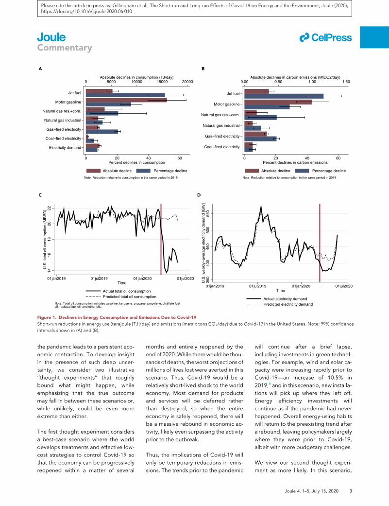
Figure 1 displays the results. (A) shows

that the largest percentage declines in

energy consumption are from jet fuel

and gasoline, with reductions of 50%

and 30% that appear persistent (see

C for overall oil consumption over

time), in line with estimates of per-

sonal vehicle travel.1 In contrast,

most other categories have observed

smaller reductions. Use of natural gas

in residential and commercial build-

ings has declined by almost 20%,

while overall electricity demand (and

demand for coal-fired electricity) has

declined by less than 10%. While com-

mercial and industrial electricity use

may have been affected by the shut-

downs, some of the decline was offset

by increased residential electricity

demand from people staying at

home, and by June, electricity con-

sumption has largely returned to the

trend (D).2

(B) illustrates the declines in CO2 emis-

sions corresponding to the reductions

in energy use. The largest reductions

are in gasoline, but the natural gas

decline leads to nearly as large a

reduction in CO2 emissions as for jet

fuel. These reductions imply a roughly

15% total reduction in daily CO2 emis-

sions, which will be the largest annual

percentage decline for the United

States in recorded history should this

drop continue. For context, the

decline in CO2 emissions is in line

with the declines laid out in the

2025 U.S. Nationally Determined Con-

tributions under the Paris Agreement,

but the sources of the decrease are

entirely different than would be ex-

pected under an optimal emissions

reduction strategy focusing on both

behavioral and structural changes to

the energy system. Other estimates

tend to focus on the world rather

than the United States or do not cover

all fuels. While estimates for the

United States cover a very wide range,

our finding is similar to the 17% global

decline in CO2 emissions for the

period through April 2020.3

The reductions in energy demand are

also reducing emissions of local air pol-

lutants that affect near-term human

health. We calculate the reductions in

SO2, nitrogen oxides (NOx), volatile

organic compounds (VOCs), and partic-

ular matter (PM) emissions (see Supple-

mental Information for details). The re-

ductions range from 12% for NOx to

1% for PM. We estimate that the shut-

downs save about 200 lives per month,

primarily driven by the lower PM emis-

sions from transportation. Of course,

these are small consolations for the

over 100,000 confirmed deaths due to

Covid-19 before June 2020.

Along with the reduction in driving from

the shutdowns has also come a decline

in traffic accidents and congestion. For

example, the number of crashes over

the period of March 13, 2020 to early

April are less than half of the previous

year, although fatal crashes did not

decline by as much, perhaps due to

the remaining vehicles being driven

longer (see Supplemental Information).

There is also a more subtle impact due

to the shutdowns: most investment in

the low-carbon transition has come to

a halt. Global electric vehicle sales are

projected to decline by 43% in 20204

due to the plummeting auto sales over-

all combined with low gasoline prices.

New residential rooftop solar and stor-

age installations have plummeted, as

have energy efficiency audits. Even at

the utility scale, renewable develop-

ments have been slowed. Overall clean

energy jobs dropped by almost

600,000 by the end of April.5 While

these are short-run impacts, they may

have long-run effects.

Long-run Effects

While the short-run effects of Covid-19

are already clear, the long-run effects

are highly uncertain. How the pandemic

influences emissions and health out-

comes in the long run depends

on how long it takes to bring the

pandemic under control and whether

Jet fuel

Motor gasoline

Natural gas res.+com.

Natural gas industrial

Gas−fired electricity

Coal−fired electricity

Electricity demand

0 5000 10000 15000 20000Absolute declines in consumption (TJ/day)

0 20 40 60Percent declines in consumption

Absolute decline Percentage decline

Note: Reduction relative to consumption in the same period in 2019

A

Jet fuel

Motor gasoline



Gas−fired electricity

Coal−fired electricity

0.00 0.50 1.00 1.50Absolute declines in carbon emissions (MtCO2/day)

0 20 40 60Percent declines in carbon emissions

Absolute decline Percentage decline


B

1416

1820

22U

.S. t

otal

oil

cons

umpt

ion

(MB

BD

)

01jan2019 01jul2019 01jan2020 01jul2020Time

Actual total oil consumptionPredicted total oil consumption

Note: Total oil consumption includes gasoline, kerosene, propane, propylene, distillate fueloil, residual fuel oil, and other oils.

C

350

400

450

500

550

U.S

. wee

kly−

aver

age

elec

tric

ity d

eman

d [G

W]

01jan2019 01jul2019 01jan2020 01jul2020Time

Actual electricity demandPredicted electricity demand

D

Figure 1. Declines in Energy Consumption and Emissions Due to Covid-19

Short-run reductions in energy use (terajoule [TJ]/day) and emissions (metric tons CO2/day) due to Covid-19 in the United States. Note: 99% confidence

intervals shown in (A) and (B).

ll


Commentary

the pandemic leads to a persistent eco-

nomic contraction. To develop insight

in the presence of such deep uncer-

tainty, we consider two illustrative

‘‘thought experiments’’ that roughly

bound what might happen, while

emphasizing that the true outcome

may fall in between these scenarios or,

while unlikely, could be even more

extreme than either.

The first thought experiment considers

a best-case scenario where the world

develops treatments and effective low-

cost strategies to control Covid-19 so

that the economy can be progressively

reopened within a matter of several

months and entirely reopened by the

end of 2020.While therewould be thou-

sands of deaths, theworst projections of

millions of lives lost were averted in this

scenario. Thus, Covid-19 would be a

relatively short-lived shock to the world

economy. Most demand for products

and services will be deferred rather

than destroyed, so when the entire

economy is safely reopened, there will

be a massive rebound in economic ac-

tivity, likely even surpassing the activity

prior to the outbreak.

Thus, the implications of Covid-19 will

only be temporary reductions in emis-

sions. The trends prior to the pandemic

will continue after a brief lapse,

including investments in green technol-

ogies. For example, wind and solar ca-

pacity were increasing rapidly prior to

Covid-19—an increase of 10.5% in

2019,6 and in this scenario, new installa-

tions will pick up where they left off.

Energy efficiency investments will

continue as if the pandemic had never

happened. Overall energy-using habits

will return to the preexisting trend after

a rebound, leaving policymakers largely

where they were prior to Covid-19,

albeit with more budgetary challenges.

We view our second thought experi-

ment as more likely. In this scenario,

Joule 4, 1–5, July 15, 2020 3

750

850

950

1050

1150

2019 2020 2021 2022 2023 2024 2025 2026 2027 2028 2029 2030 2031 2032 2033 2034 2035

AEO 2020 Reference Case One-quarter Shutdown Two-quarter Shutdown

1250

1350

1450

1550

1650

2019 2020 2021 2022 2023 2024 2025 2026 2027 2028 2029 2030 2031 2032 2033 2034 2035

AEO 2020 Reference Case One-quarter Shutdown Two-quarter Shutdown

A

B

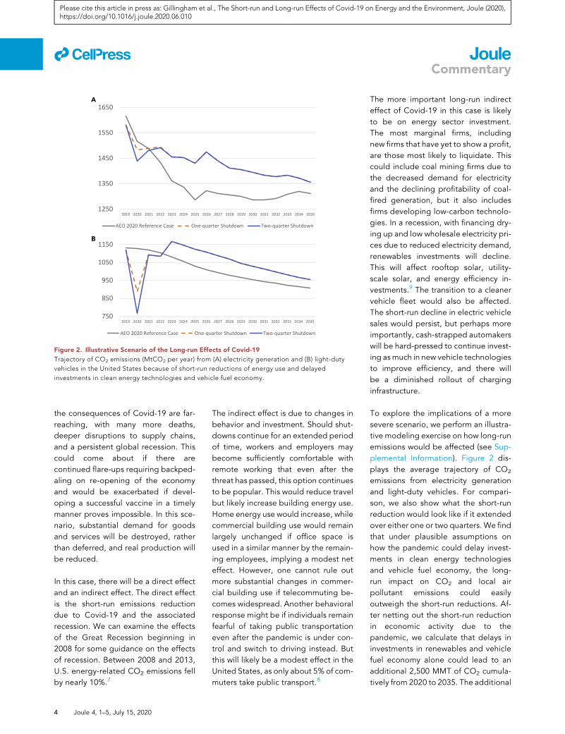
Figure 2. Illustrative Scenario of the Long-run Effects of Covid-19

Trajectory of CO2 emissions (MtCO2 per year) from (A) electricity generation and (B) light-duty

vehicles in the United States because of short-run reductions of energy use and delayed

investments in clean energy technologies and vehicle fuel economy.

ll


Commentary

the consequences of Covid-19 are far-

reaching, with many more deaths,

deeper disruptions to supply chains,

and a persistent global recession. This

could come about if there are

continued flare-ups requiring backped-

aling on re-opening of the economy

and would be exacerbated if devel-

oping a successful vaccine in a timely

manner proves impossible. In this sce-

nario, substantial demand for goods

and services will be destroyed, rather

than deferred, and real production will

be reduced.

In this case, there will be a direct effect

and an indirect effect. The direct effect

is the short-run emissions reduction

due to Covid-19 and the associated

recession. We can examine the effects

of the Great Recession beginning in

2008 for some guidance on the effects

of recession. Between 2008 and 2013,

U.S. energy-related CO2 emissions fell

by nearly 10%.7

4 Joule 4, 1–5, July 15, 2020

The indirect effect is due to changes in

behavior and investment. Should shut-

downs continue for an extended period

of time, workers and employers may

become sufficiently comfortable with

remote working that even after the

threat has passed, this option continues

to be popular. This would reduce travel

but likely increase building energy use.

Home energy use would increase, while

commercial building use would remain

largely unchanged if office space is

used in a similar manner by the remain-

ing employees, implying a modest net

effect. However, one cannot rule out

more substantial changes in commer-

cial building use if telecommuting be-

comes widespread. Another behavioral

response might be if individuals remain

fearful of taking public transportation

even after the pandemic is under con-

trol and switch to driving instead. But

this will likely be a modest effect in the

United States, as only about 5% of com-

muters take public transport.8

The more important long-run indirect

effect of Covid-19 in this case is likely

to be on energy sector investment.

The most marginal firms, including

new firms that have yet to show a profit,

are those most likely to liquidate. This

could include coal mining firms due to

the decreased demand for electricity

and the declining profitability of coal-

fired generation, but it also includes

firms developing low-carbon technolo-

gies. In a recession, with financing dry-

ing up and low wholesale electricity pri-

ces due to reduced electricity demand,

renewables investments will decline.

This will affect rooftop solar, utility-

scale solar, and energy efficiency in-

vestments.9 The transition to a cleaner

vehicle fleet would also be affected.

The short-run decline in electric vehicle

sales would persist, but perhaps more

importantly, cash-strapped automakers

will be hard-pressed to continue invest-

ing asmuch in new vehicle technologies

to improve efficiency, and there will

be a diminished rollout of charging

infrastructure.

To explore the implications of a more

severe scenario, we perform an illustra-

tive modeling exercise on how long-run

emissions would be affected (see Sup-

plemental Information). Figure 2 dis-

plays the average trajectory of CO2

emissions from electricity generation

and light-duty vehicles. For compari-

son, we also show what the short-run

reduction would look like if it extended

over either one or two quarters. We find

that under plausible assumptions on

how the pandemic could delay invest-

ments in clean energy technologies

and vehicle fuel economy, the long-

run impact on CO2 and local air

pollutant emissions could easily

outweigh the short-run reductions. Af-

ter netting out the short-run reduction

in economic activity due to the

pandemic, we calculate that delays in

investments in renewables and vehicle

fuel economy alone could lead to an

additional 2,500 MMT of CO2 cumula-

tively from 2020 to 2035. The additional

ll


Commentary

local air pollutants could lead to 40

deaths per month on average, or

7,500 deaths, from 2020 to 2035. In

our simulations, we assume no perma-

nent changes to consumption from the

pandemic. But we calculate that if there

are such changes, they would need to

be large—at least 4% of total energy-

related emissions—to compensate

for the delayed investment. Similarly,

coal retirements would have to more

than double from pre-pandemic

forecasts to offset the delayed renew-

ables investment (see Supplemental

Information).

Our findings suggest that even just

pushing back all renewable electricity

generation investments by one year

would outweigh the emissions reduc-

tions and avoided deaths from March

to June of 2020. However, the energy

policy response to Covid-19 is the wild

card that can change everything.

Implications for Policy

Even if the world does face our second

thought experiment, long-run emission

increases are not preordained. The

government policy response is

crucial.10 And there is a real reason to

be concerned. Government budgets

are going to be stretched thin in paying

for the costs of Covid-19, making it

more difficult to invest in clean energy

and public transportation. Further-

more, if the economy remains in a

persistent recession, there may be

intense pressure to relax climate

change mitigation targets. But there is

also an opportunity.

Many nations around the world,

including those in the EU, UK, Japan,

and South Korea, are considering stim-

ulus packages explicitly focusing on

clean energy. But in the United States,

it is unlikely that clean technology and

infrastructure will be at the heart of

any stimulus package in the near future

even if that possibility cannot be ruled

out. The American Recovery and Rein-

vestment Act stimulus package in

2009 allocated sums toward clean en-

ergy investment, and similar invest-

ments are in the policy debate.11 Even

a modest allocation toward new tech-

nologies may pay dividends in the

future in terms of clean air, clean jobs,

and national security.12 But simply sta-

bilizing the economy would be valuable

for putting the trends toward clean en-

ergy back on track.

At the state level, there may be more

room for policy action. If financing

dries up for new investment in renew-

ables, state green banks can help

bridge the gap. States can also expe-

dite permitting, while of course retain-

ing environmental and other safe-

guards. Covid-19 may also remind

voters and policymakers that collective

action and listening to scientists mat-

ters, leading to greater efforts on pol-

icy to reduce emissions, possibly even

including carbon pricing. The research

community could start new endeavors

analyzing potential policy options to

help bring us out of the malaise of

Covid-19. These developments would

be a true ‘‘silver lining’’ to the Covid-

19 crisis.

Data and Code Availability

The data and code reported in this pa-

per have been deposited in Github,

https://github.com/MartenOvaere/

energy_longruneffects_covid19_Joule.

SUPPLEMENTAL INFORMATION

Supplemental Information can be

found online at https://doi.org/10.

1016/j.joule.2020.06.010.

1. Cicala, S., Holland, S.P., Mansur, E.T., Muller,N.Z., and Yates A.J. (2020). Expected HealthEffects of Reduced Air Pollution fromCOVID-19 Social Distancing.

2. NYISO (2020). New York IndependentSystem Operator Covid-19 Updates. https://www.nyiso.com/covid.

3. Quere, C.L., Jackson, R.B., Jones, M.W.,Smith, A.J.P., Abernethy, S., Andrew, R.M.,De-Gol, A.J., Willis, D.R., Shan, Y., Canadell,J.G., et al. (2020). Temporary Reduction inDaily Global CO2 Emissions during theCOVID-19 Forced Confinement. Nat. Clim.Chang. https://doi.org/10.1038/s41558-020-0797-x.

4. WoodMac (2020). Global Electric VehicleSales to Drop 43% in 2020. https://www.woodmac.com/press-releases/global-electric-vehicle-sales-to-drop-43-in-2020/.

5. BW Research Partnership (2020). CleanEnergy Employment Initial Impacts from theCOVID-19 Economic Crisis. https://e2.org/wp-content/uploads/2020/05/Clean-Energy-Jobs-April-COVID-19-Memo-FINAL.pdf.

6. EIA (2020a). Electric Power Monthly. https://www.eia.gov/electricity/monthly/.

7. EIA (2020b). Monthly Energy Review. https://www.eia.gov/totalenergy/data/browser/.

8. DOT (2016). National TransportationStatistics. Table 1-41. https://www.bts.gov/content/commute-mode-share-2015.

9. IEA (2020). Renewable Energy MarketUpdate: Outlook for 2020 and 2021. https://www.iea.org/reports/renewable-energy-market-update/covid-19-impact-on-renewable-energy-growth.

10. Steffen, B., Egli, F., Pahle, M., and Schmidt,T.S. (2020). Navigating the Clean EnergyTransition in the COVID-19 Crisis (Joule).https://doi.org/10.1016/j.joule.2020.04.011.

11. CEA (2016). A Retrospective Assessment ofClean Energy Investments in the RecoveryAct. White House Council of EconomicAdvisers. https://obamawhitehouse.archives.gov/sites/default/files/page/files/20160225_cea_final_clean_energy_report.pdf.

12. Baker, J., Shultz, G., and Halstead, T. (2020).The Strategic Case for U.S. ClimateLeadership. Foreign Affairs. https://www.foreignaffairs.com/articles/united-states/2020-04-13/strategic-case-us-climate-leadership.

1Yale University andNational Bureau of EconomicResearch, 195 Prospect Street, New Haven, CT06511, USA

2MIT Sloan School of Management and NationalBureau of Economic Research, 100 Main Street,Cambridge, MA 02142, USA

3MIT Sloan School of Management, 100 MainStreet, Cambridge, MA 02142, USA

4Yale University, 195 Prospect Street, New Haven,CT 06511, USA

5Northwestern University Department ofEconomics and National Bureau of EconomicResearch, 2211 Campus Drive, 3rd Floor,Evanston, IL 60208, USA

*Correspondence: [email protected]

https://doi.org/10.1016/j.joule.2020.06.010

Joule 4, 1–5, July 15, 2020 5

https://github.com/MartenOvaere/energy_longruneffects_covid19_Joule

https://github.com/MartenOvaere/energy_longruneffects_covid19_Joule



https://www.nyiso.com/covid

https://www.nyiso.com/covid

https://doi.org/10.1038/s41558-020-0797-x

https://doi.org/10.1038/s41558-020-0797-x

https://www.woodmac.com/press-releases/global-electric-vehicle-sales-to-drop-43-in-2020/



https://e2.org/wp-content/uploads/2020/05/Clean-Energy-Jobs-April-COVID-19-Memo-FINAL.pdf




https://www.eia.gov/electricity/monthly/

https://www.eia.gov/electricity/monthly/

https://www.eia.gov/totalenergy/data/browser/

https://www.eia.gov/totalenergy/data/browser/

https://www.bts.gov/content/commute-mode-share-2015

https://www.bts.gov/content/commute-mode-share-2015

https://www.iea.org/reports/renewable-energy-market-update/covid-19-impact-on-renewable-energy-growth





https://obamawhitehouse.archives.gov/sites/default/files/page/files/20160225_cea_final_clean_energy_report.pdf




https://www.foreignaffairs.com/articles/united-states/2020-04-13/strategic-case-us-climate-leadership




mailto:[email protected]


JOUL, Volume 4

Supplemental Information

The Short-run

and Long-run

Effects

of Covid-19

on Energy

and the

Environment

Kenneth T. Gillingham, Christopher R. Knittel, Jing Li, Marten Ovaere, and Mar Reguant

1

1 Decreased energy consumption

1.1 Data

Table 1 presents the time period, frequency and source of the U.S. energy consumption data used in this study. A long time series of weekly oil data is available, while data of weekly natural gas consumption and hourly electricity consumption and generation is only available from 2017 and 2019.

Table 1: Source, time period and frequency of data on U.S. energy consumption.

Energy source Time period Frequency Units Source

Petroleum and other liquids

2001-2020 Weekly 1000 B/D (U.S. Energy Information Administration 2020d)

Natural gas 2017-2020 Weekly Bcf/D (U.S. Energy Information Administration 2020c)

Electricity demand 2019-2020 Hourly MW (U.S. Energy Information Administration 2020b)

Electricity generation 2019-2020 Hourly MW (U.S. Energy Information Administration

2020b)

We also use U.S. heating and cooling degree day data from U.S. National Oceanic and Atmospheric Administration (2020), to control for the effect of temperature on gas and coal consumption from heating and electricity demand. Electricity demand and generation are aggregated to daily data, while heating and cooling degree day data are aggregated to weekly data when used in the weekly oil and natural gas data.

1.2 Empirical specifications

We estimate the coefficient βCOVID on a COVID dummy that is equal to one on all days or weeks of data after March 25, 2020. This is the week starting on March 26 for natural gas and the week starting on March 28 for oil. We use ten weeks of post-shutdown data, until June 7, 2020.

Following Hausman and Rapson (2018), we run both a global polynomial regression and a

two-step augmented local regression to estimate the effect of the COVID-19 measures on energy consumption. In the global polynomial regression, we estimate βCOVID in the full data sample (see second column of Table 1), while controlling for weather and seasonality. In the augmented local regression, on the other hand, we first estimate the impacts of weather, seasonality and other controls in the sample ending three weeks before the start of shutdowns, using the following empirical specifications for oil (1), natural gas (2), electricity generation (3) and electricity demand (4):

qfuel,t = δt + εt for fuel = {gasoline, kerosene} (1)

= hddt + cddt + εt for fuel = {res.+com., industrial, total} (2)

= hddt + cddt + qsolar,t + qwind,t + εt for fuel = {coal, gas, nuclear, hydro} (3)

= hddt + cddt + εt for fuel = {electricity demand} (4)

where qfuel,it is the fuel consumption at week or day t, while δt are week fixed-effects to control for regular patterns in oil consumption. Because the time period for natural gas and electricity is much shorter, we do not use fixed effects, but hddt and cddt are the number of heating and cooling degree days in day or week t, to control for the effect of temperatures on natural gas and electricity demand.

2

We also include daily solar and wind electricity generation, which are determined by exogenous changes in wind speed and solar irradiance.

In a second step, βCOVID is estimated as the difference of first-stage residuals in a narrow bandwidth around the discontinuity (March 26th, 2020). We again ignore three weeks of data before the discontinuity to mitigate concerns of behavioral change before official shutdown measures started. The global polynomial and augmented local regression lead to very similar results (see supplemental estimation file), so we present the results of the augmented local regression.

1.3 Results

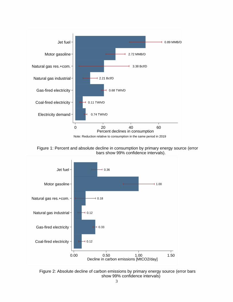
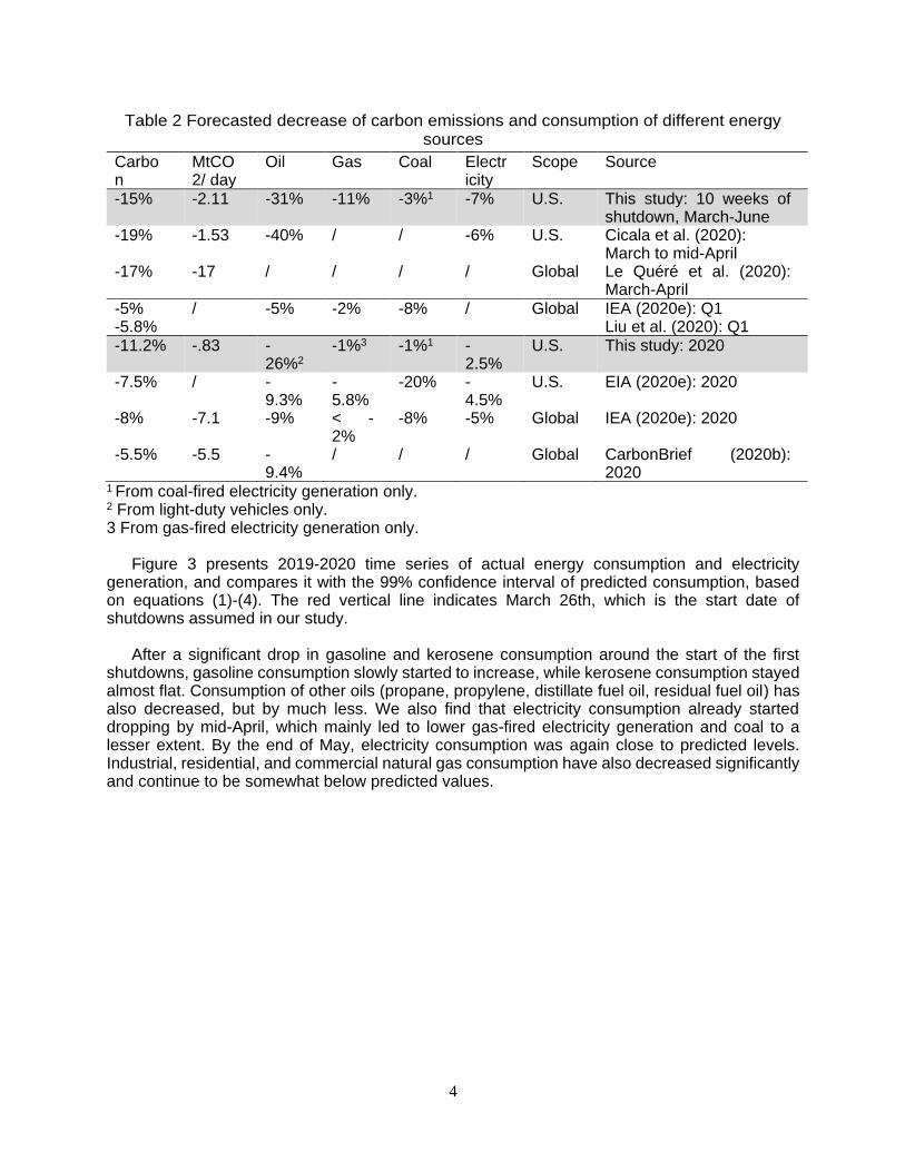
Panel a of Figure 1 in the main text presents the results of the above estimation for every major energy source. Jet fuel consumption has decreased most in relative terms, while motor gasoline consumption has decreased most in absolute terms. Multiplying these estimates by carbon emission factors (see Table 2), panel b of this figure presents the decline of daily carbon emissions in million tons. Total carbon emissions decreased by around 20% for our studied energy sources, in line with the 25% decrease (200 MtCO2) of China’s carbon emissions in the first four weeks after shutdowns (CarbonBrief, 2020a). Figure 1 and Figure 2 below present similar figures but show the absolute numbers in their original units: MMB/D, Bcf/D and TWh/D. Table 2 compares our estimates of decreased energy consumption and associated carbon emissions with three types of recent reports. First, two recent studies look at the changes in energy consumption and emissions during shutdowns. Our short-term estimates of total carbon emissions (first row) are the most similar to Cicala et al., (2020) and Le Quéré et al., (2020). However, we estimate changes in primary energy consumption of oil and gas, and gas- and coal-fired electricity generation based on detailed U.S. data, while Le Quéré et al. (2020) estimate worldwide demand reductions using consumption proxies by sector and multiplying them by the average carbon emission intensity per sector. Cicala et al. (2020) do not estimate the effect on consumption of natural gas and coal, but their estimate of oil and electricity are very similar – although though we consider a much longer lockdown period. Other estimates are more different. IEA (2020e) and Liu et al. (2020) present estimates of average emission reductions over the first quarter of 2020, so their results are for a different time period and thus are difficult to compare to ours. Our overall 2020 illustrative predictions (sixth row) are somewhat different than other studies. However, in our long-run analysis, we focus on light-duty vehicles and electricity, and assume a larger negative effect on renewable investment in our worst-case long-run scenario than in other reports. In addition, our short-term estimates and 2020 forecasts are relative to business-as-usual 2020 projections, while EIA (2020e) compares to 2019 values, which may not be an appropriate baseline. See section 5 of the SM for more information.

3

Figure 1: Percent and absolute decline in consumption by primary energy source (error bars show 99% confidence intervals).

Figure 2: Absolute decline of carbon emissions by primary energy source (error bars show 99% confidence intervals)

2.72 MMB/D

0.89 MMB/D

3.38 Bcf/D

2.21 Bcf/D

0.74 TWh/D

0.68 TWh/D

0.11 TWh/D

Jet fuel

Motor gasoline



Gas-fired electricity

Coal-fired electricity

Electricity demand

0 20 40 60Percent declines in consumption


1.00

0.36

0.18

0.12

0.33

0.12

Jet fuel

Motor gasoline





0.00 0.50 1.00 1.50Decline in carbon emissions [MtCO2/day]

4

Table 2 Forecasted decrease of carbon emissions and consumption of different energy sources

Carbon

MtCO2/ day

Oil Gas Coal Electricity

Scope Source

-15% -2.11 -31% -11% -3%1 -7% U.S. This study: 10 weeks of shutdown, March-June

-19% -1.53 -40% / / -6% U.S. Cicala et al. (2020): March to mid-April

-17% -17 / / / / Global Le Quéré et al. (2020): March-April

-5% / -5% -2% -8% / Global IEA (2020e): Q1 -5.8% Liu et al. (2020): Q1 -11.2% -.83 -

26%2 -1%3 -1%1 -

2.5% U.S. This study: 2020

-7.5% / -9.3%

-5.8%

-20% -4.5%

U.S. EIA (2020e): 2020

-8% -7.1 -9% < -2%

-8% -5% Global IEA (2020e): 2020

-5.5% -5.5 -9.4%

/ / / Global CarbonBrief (2020b): 2020

1 From coal-fired electricity generation only. 2 From light-duty vehicles only. 3 From gas-fired electricity generation only.

Figure 3 presents 2019-2020 time series of actual energy consumption and electricity

generation, and compares it with the 99% confidence interval of predicted consumption, based on equations (1)-(4). The red vertical line indicates March 26th, which is the start date of shutdowns assumed in our study.

After a significant drop in gasoline and kerosene consumption around the start of the first

shutdowns, gasoline consumption slowly started to increase, while kerosene consumption stayed almost flat. Consumption of other oils (propane, propylene, distillate fuel oil, residual fuel oil) has also decreased, but by much less. We also find that electricity consumption already started dropping by mid-April, which mainly led to lower gas-fired electricity generation and coal to a lesser extent. By the end of May, electricity consumption was again close to predicted levels. Industrial, residential, and commercial natural gas consumption have also decreased significantly and continue to be somewhat below predicted values.

5

Figure 3: Comparing actual energy consumption and electricity generation with the 99% confidence interval of expected consumption in our model.

6

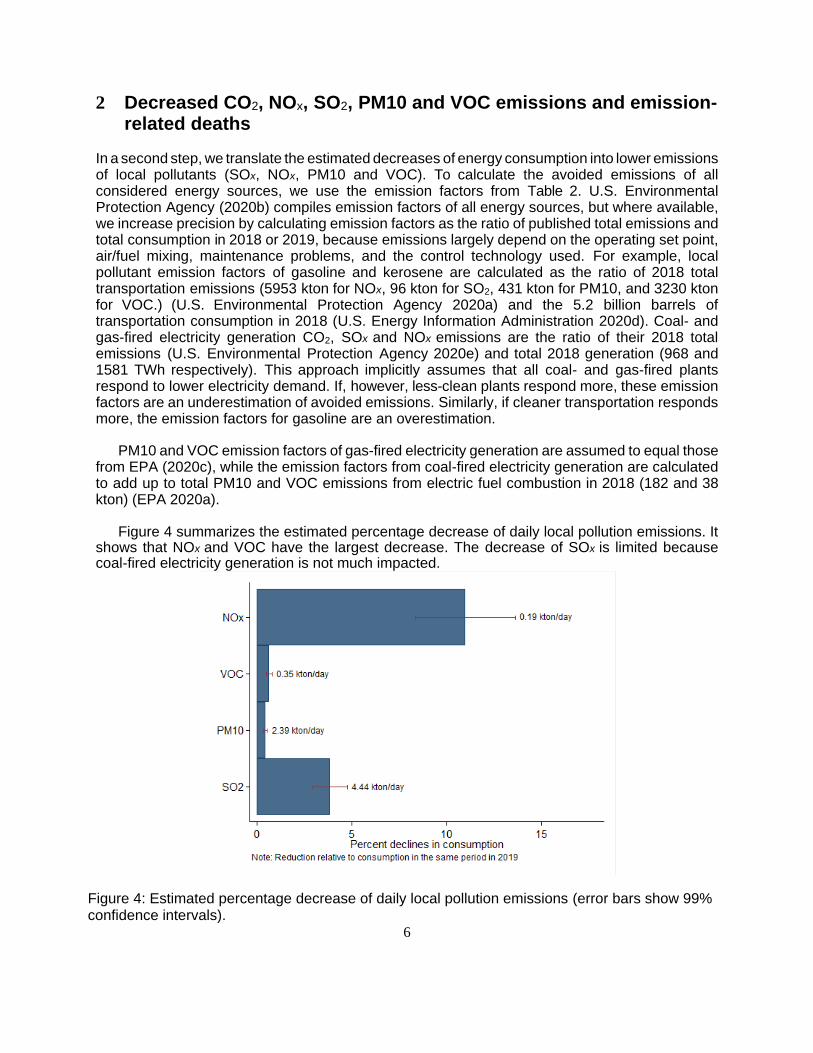
2 Decreased CO2, NOx, SO2, PM10 and VOC emissions and emission-related deaths

In a second step, we translate the estimated decreases of energy consumption into lower emissions of local pollutants (SOx, NOx, PM10 and VOC). To calculate the avoided emissions of all considered energy sources, we use the emission factors from Table 2. U.S. Environmental Protection Agency (2020b) compiles emission factors of all energy sources, but where available, we increase precision by calculating emission factors as the ratio of published total emissions and total consumption in 2018 or 2019, because emissions largely depend on the operating set point, air/fuel mixing, maintenance problems, and the control technology used. For example, local pollutant emission factors of gasoline and kerosene are calculated as the ratio of 2018 total transportation emissions (5953 kton for NOx, 96 kton for SO2, 431 kton for PM10, and 3230 kton for VOC.) (U.S. Environmental Protection Agency 2020a) and the 5.2 billion barrels of transportation consumption in 2018 (U.S. Energy Information Administration 2020d). Coal- and gas-fired electricity generation CO2, SOx and NOx emissions are the ratio of their 2018 total emissions (U.S. Environmental Protection Agency 2020e) and total 2018 generation (968 and 1581 TWh respectively). This approach implicitly assumes that all coal- and gas-fired plants respond to lower electricity demand. If, however, less-clean plants respond more, these emission factors are an underestimation of avoided emissions. Similarly, if cleaner transportation responds more, the emission factors for gasoline are an overestimation.

PM10 and VOC emission factors of gas-fired electricity generation are assumed to equal those from EPA (2020c), while the emission factors from coal-fired electricity generation are calculated to add up to total PM10 and VOC emissions from electric fuel combustion in 2018 (182 and 38 kton) (EPA 2020a).

Figure 4 summarizes the estimated percentage decrease of daily local pollution emissions. It

shows that NOx and VOC have the largest decrease. The decrease of SOx is limited because coal-fired electricity generation is not much impacted.

Figure 4: Estimated percentage decrease of daily local pollution emissions (error bars show 99% confidence intervals).

7

Table 3: Assumed emission factors of considered energy sources.

Energy source Emission factor Source

Gasoline [kg/barrel]

CO2 369 (U.S. Energy Information Administration 2020a)

SOx 0.018 (U.S. Environmental Protection Agency 2020a)

NOx 1.145 (U.S. Environmental Protection Agency 2020a)

PM10 0.083 (U.S. Environmental Protection Agency 2020a)

VOC 0.621 (U.S. Environmental Protection Agency 2020a)

Kerosene [kg/barrel]

CO2 402 (U.S. Energy Information Administration 2020a)

SOx 0.018 (U.S. Environmental Protection Agency 2020a)

NOx 1.145 (U.S. Environmental Protection Agency 2020a)



Gas-fired electricity generation [kg/MWh]

CO2 480 (U.S. Environmental Protection Agency 2020e)

SOx 0.012 (U.S. Environmental Protection Agency 2020e)

NOx 0.118 (U.S. Environmental Protection Agency 2020e)

PM10 0.026 (U.S. Environmental Protection Agency 2020c)

VOC 0.019 (U.S. Environmental Protection Agency 2020c)

Coal-fired electricity generation [kg/MWh]

CO2 1090 (U.S. Environmental Protection Agency 2020e)

SOx 0.983 (U.S. Environmental Protection Agency 2020e)

NOx 0.724 (U.S. Environmental Protection Agency 2020e)



Residential, commercial (heating) and industrial natural gas [kg/MMcf]

CO2 53,120 (U.S. Energy Information Administration 2020a)

SOx 0.27 (U.S. Environmental Protection Agency 2020c)

NOx 23 (U.S. Environmental Protection Agency 2020c)

PM10 3.5 (U.S. Environmental Protection Agency 2020c)

VOC 2.5 (U.S. Environmental Protection Agency 2020c)

8

In a next step, we calculate the number of avoided deaths because of lower local pollution

emissions. Using the mortality factors of table 3 (Muller 2014; Muller et al. 2011), Figure 5 presents

the number of avoided deaths per month for the duration of the current shutdown measures. Our

approach for U.S. total consumption and emissions implicitly assumes that emissions decrease

uniformly across the U.S. This is a conservative estimate, given that the decrease of jet fuel and

motor gasoline is larger in densely populated areas. To study the geographical distribution of local

pollution in more detail, the next section looks at the concentration of PM2.5 across different monitors

in the United States.

Table 4: Deaths per 1000 tons of pollutant emissions in the U.S. (Muller 2014; Muller et al. 2011).

Pollutant Deaths per 1000 tons

SOx 2.7486

NOx 0.2912

PM10 7.9521

VOC 0.6924

Figure 5: Avoided deaths per month because of the estimated decrease emissions of local pollutants (error bars show 99% confidence intervals).

133

39

3

2

5

6

Jet fuel

Motor gasoline





0 50 100 150 200Decline in emissions-related deaths per month

9

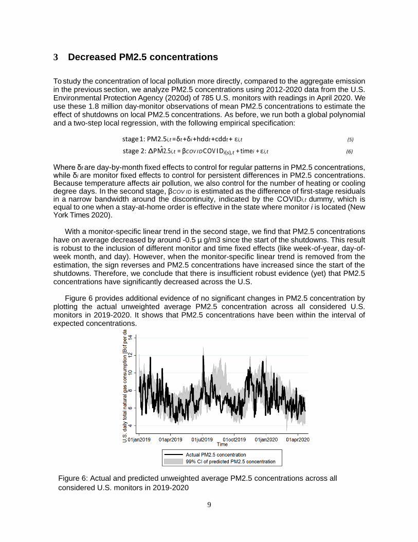
3 Decreased PM2.5 concentrations

To study the concentration of local pollution more directly, compared to the aggregate emission in the previous section, we analyze PM2.5 concentrations using 2012-2020 data from the U.S. Environmental Protection Agency (2020d) of 785 U.S. monitors with readings in April 2020. We use these 1.8 million day-monitor observations of mean PM2.5 concentrations to estimate the effect of shutdowns on local PM2.5 concentrations. As before, we run both a global polynomial and a two-step local regression, with the following empirical specification:

stage 1: P M 2.5i,t = δt + δi + hddt + cddt + εi,t (5)

stage 2: ∆P M2.5i,t = βCOV IDCOV IDi(s),t + timei + εi,t (6)

Where δt are day-by-month fixed effects to control for regular patterns in PM2.5 concentrations, while δi are monitor fixed effects to control for persistent differences in PM2.5 concentrations. Because temperature affects air pollution, we also control for the number of heating or cooling degree days. In the second stage, βCOV ID is estimated as the difference of first-stage residuals in a narrow bandwidth around the discontinuity, indicated by the COVIDi,t dummy, which is equal to one when a stay-at-home order is effective in the state where monitor i is located (New York Times 2020).

With a monitor-specific linear trend in the second stage, we find that PM2.5 concentrations

have on average decreased by around -0.5 µ g/m3 since the start of the shutdowns. This result is robust to the inclusion of different monitor and time fixed effects (like week-of-year, day-of-week month, and day). However, when the monitor-specific linear trend is removed from the estimation, the sign reverses and PM2.5 concentrations have increased since the start of the shutdowns. Therefore, we conclude that there is insufficient robust evidence (yet) that PM2.5 concentrations have significantly decreased across the U.S.

Figure 6 provides additional evidence of no significant changes in PM2.5 concentration by plotting the actual unweighted average PM2.5 concentration across all considered U.S. monitors in 2019-2020. It shows that PM2.5 concentrations have been within the interval of expected concentrations.

Figure 6: Actual and predicted unweighted average PM2.5 concentrations across all

considered U.S. monitors in 2019-2020

10

U.S. Environmental Protection Agency (2020d) has data on concentrations of other local pollutants like SO2 and NO2, but at the time of writing this article, March and April 2020 data were not yet available. However, news articles have cited proprietary sources to suggest up to 31% decline of NO2 in some urban areas, such as San Francisco (Wall Street Journal 2020).

4 Reductions in Vehicle Crashes

4.1 Data Sources

Along with reduced driving should come reductions in vehicle crashes. We drew upon detailed

crash records from several states that have publicly available data.

The latest detailed crash records were available at the state/city level for Utah, Massachusetts,

Iowa, California and New York city. This data is comprised of vehicle/person level crash entries

and includes any collision that resulted in an injury, death or property value exceeding

$1000/$1500 depending on the reporting authority.

NYC data:

Extracted from NYC Open Data portal:

https://data.cityofnewyork.us/Public-Safety/Motor-Vehicle-Collisions-Vehicles/bm4k-52h4

Series: Motor Vehicles Collisions – Vehicles

Data provided by: Police Department (NYPD)

Description: The Motor Vehicle Collisions vehicle table contains details on each vehicle involved

in the crash. Each row represents a motor vehicle involved in a crash. It includes all crashes

where there was an injury, a death or at least $1000 worth of property damage.

Received/requested on: 04/01/2020

Timespan we use: 01/01/2019-03/28/2020

Utah:

Requested from the Department of Public Safety, State of Utah

https://highwaysafety.utah.gov/crash-data/

Timespan we use:

Description: The data contains details on each crash and people involved. Information is collected

when a crash involves injuries, deaths or at least $1,500 worth of property damage.


Timespan we use: 01/01/2019-03/30/2020

Massachusetts:

Extracted from: MassDOT IMPACT Open Data

https://massdot-impact-crashes-vhb.opendata.arcgis.com/datasets/2020-person-level-crash-

details

https://massdot-impact-crashes-vhb.opendata.arcgis.com/datasets/2019-person-level-crash-

details-

Provided by: Massachusetts Deparment of Transportation

Description: The data contains details on each crash and people involved. Information is collected

when a crash involves injuries, deaths or at least $1,000 worth of property damage.

https://massdot-impact-crashes-vhb.opendata.arcgis.com/datasets/2020-person-level-crash-details

https://massdot-impact-crashes-vhb.opendata.arcgis.com/datasets/2020-person-level-crash-details

11


Timespan we use: 01/01/2019-04/17/2020

Iowa:

Extracted from: ICAT – Iowa Crash Analysis Tool

https://icat.iowadot.gov/

Provided by: Iowa Department of Transportation

Records crashes that have resulted in an injury/fatality or the estimated property damage of the

crash is equal to or greater than $1,500.


Timespan we use: 01/01/2019-04/03/2020

California:

Extracted from:

http://iswitrs.chp.ca.gov/Reports/jsp/userLogin.jsp

Series comes from: The Statewide Integrated Traffic Records System (SWITRS)

Provided by: California Highway patrol

Records crashes that have resulted in an injury/fatality or the estimated property damage of the

crash is equal to or greater than $1,000.


Timespan we use: 01/01/2019-04/09/2020

4.2 Analysis

For initial descriptive evidence, we began by plotting the ratio of total traffic crashes in 2020 to

the same time period in 2019 at the daily level. This is below in Figure 7. We observe a slight

downward trend after February 26th, which is the date thought at the time to be the first Covid-19

death in the United States and a clearer downward trend after March 13th when President Trump

declared a national emergency. The average pre-February 26th ratio is just below 1, while the

average post-March 13th ratio is 0.41 when averaged across all of these regions.

12

Figure 7: Seven-day moving average of the ratio of 2020 to 2019 crashes by state or region.

Numbers greater than 1 indicate more crashes in 2020, while less than 1 indicate fewer

crashes in 2020. The dotted line refers to February 26, while the shaded area includes all

days after March 13th.

We can create a similar figure for crash fatalities. Figure 8 shows this figure, which plots the ratio

of crash fatalities in 2020 to 2019. The pattern is much less clear for fatalities and it is difficult to

discern a downward trend. Looking at the data, the average fatality ratio drops only very slightly

between pre-February 26th and post-March 13th. This might be due to higher speeds on roadways

with less congestion leading to more fatal crashes when crashes do occur.

13

Figure 8: Seven-day moving average of the ratio of 2020 to 2019 fatal crashes by state or

region. Numbers greater than 1 indicate more crashes in 2020, while less than 1 indicate

fewer crashes in 2020. The dotted line refers to February 26, while the shaded area includes

all days after March 13th.

We also run a set of regressions to explore the effects further using difference-in-difference or regression discontinuity designs, and find similar results – a clear effect on overall traffic crashes, but little or no effect on fatalities, depending on the specification (results are available from the authors upon request).

14

5 Long-run Impacts We develop two illustrative thought experiments to provide insight into the potential long-run impacts of Covid-19. Our philosophy in this exercise is not to exactly forecast any outcome or provide probabilities on what the outcomes might be, but rather to provide a deeper understanding of the implications of possible scenarios of what might happen. We focus on only two scenarios for greater simplicity and transparency. Our first (optimistic) thought experiment is simple: Covid-19 is brought under control quickly with treatments and/or a vaccine, and a strong economic recovery quickly comes about. This economic recovery could happen as early as the fall of 2020. This scenario does not require much modeling, as it is clear that the impacts on long run technology development will be minimal, and while there may be budgetary impacts on firms and governments, these are not so arduous as to dramatically change the flows of capital towards clean technology. Our second thought experiment is much less optimistic. It represents a case where Covid-19 is not brought under control for at least another year, and perhaps longer. The global economy goes into a deeper recession. Government budgets at all levels are strained. Many firms go bankrupt and most of those that do not are just focusing on survival, and thus are short on cash to invest in new technologies. This thought experiment might be thought of as a plausible lower-bound on what might happen, although we would like to emphasize that even worse outcomes are still possible. We view this scenario as useful for allowing us to make some illustrative quantitative estimates of what the possible implications might be, recognizing that the exact numbers are not predictions, but rather projections of a possible world intended for insight into the factors at play. Note that we do not explicitly model policy interventions in either scenario, but rather assume that policy roughly follows the pre-Covid-19 trends. Explicitly modeling the policy responses and how they affect energy use and emissions is outside the scope of this commentary, but is a valuable pathway for future research. Our modeling of the second long-run scenario consists of two main components. First, energy demand will change due to the shutdown and economic recovery in the near future. Second, fuel mixes and emissions rates will change due to possible delays in renewable technology investments and product releases, which has longer-run implications. We combine our assumptions on energy demand and emissions rates to construct potential long-run impacts on emissions. Our calculations of emissions impacts are relative to the projections in the 2020 Annual Energy Outlook (AEO) Reference Case (EIA 2020e). We recognize that there are likely to be other impacts but we view these as the largest two impacts, and thus we focus on them for our illustrative estimates. One of the more notable other possible impacts could be an accelerating of coal plant retirements, leading to a counteracting emissions decrease. This could be due to permanently lower consumption due to the pandemic. At the end of Section 5.3, we will discuss how large the emission-reducing forces would have to be to compensate for the emissions increases we model. 5.1 Short-run Change in Energy Demand: Electricity generation and light-duty vehicle miles traveled For impacts of the shutdown, we use our estimates on electricity generation, which found that electricity declined less than 10% due to the shutdown (Section 1 of the SI). Our scenario considers a strict shutdown lasting one to two quarters. We use historical data during and after

15

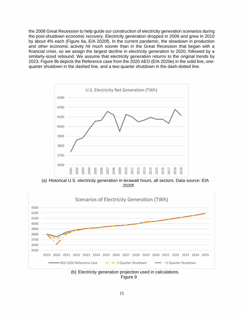
the 2008 Great Recession to help guide our construction of electricity generation scenarios during the post-shutdown economic recovery. Electricity generation dropped in 2009 and grew in 2010 by about 4% each (Figure 6a, EIA 2020f). In the current pandemic, the slowdown in production and other economic activity hit much sooner than in the Great Recession that began with a financial crisis, so we assign the largest decline in electricity generation to 2020, followed by a similarly-sized rebound. We assume that electricity generation returns to the original trends by 2023. Figure 9b depicts the Reference case from the 2020 AEO (EIA 2020e) in the solid line, one-quarter shutdown in the dashed line, and a two-quarter shutdown in the dash-dotted line.

(a) Historical U.S. electricity generation in terawatt hours, all sectors. Data source: EIA

2020f.

(b) Electricity generation projection used in calculations.

Figure 9

3600

3700

3800

3900

4000

4100

4200

4300

20

01

20

02

20

03

20

04

20

05

20

06

20

07

20

08

20

09

20

10

20

11

20

12

20

13

20

14

20

15

20

16

20

17

20

18

20

19

U.S. Electricity Net Generation (TWh)

3500

3600

3700

3800

3900

4000

4100

4200

4300

2019 2020 2021 2022 2023 2024 2025 2026 2027 2028 2029 2030 2031 2032 2033 2034 2035

Scenarios of Electricity Generation (TWh)

AEO 2020 Reference Case 1-Quarter Shutdown 2-Quarter Shutdown

16

For transportation, we focus on emissions from light-duty vehicles. Given that data on vehicle miles traveled (VMT) are not yet available from the Federal Highway Administration (FHWA), we turn to cellphone data provided by Apple Mobility Trends and Streetlight Data Inc. (See References for access information). Our scenarios consider a strict shutdown lasting one to two quarters. We again look to historical data on the Great Recession to guide our assumptions on what may happen to energy demand in transportation after the shutdown has been lifted and the economic recovery begins. Historical data on VMT in the U.S. (Figure 10a, FHWA 2020 and EIA 2020f) show that after about a 2% decline in 2008, VMT fluctuated with small increases and decreases during the recovery years afterwards.

(a) Historical U.S. vehicle miles traveled in billions of vehicle miles. Data from the FHWA are

for all traffic, while data from the EIA are for light-duty vehicles only (FHWA 2020, EIA 2014). Both data series show about a 2% drop in VMT in 2008.

2000

2200

2400

2600

2800

3000

3200

2001 2002 2003 2004 2005 2006 2007 2008 2009 2010 2011 2012 2013

United States VMT during the Great Recession and Recovery (Billion Vehicle Miles)

FHWA Travel Monitoring EIA Light-Duty Vehicles

17

(b) Light-duty VMT projection used in our calculations.

Figure 10 Driving behavior change may persist after shutdowns are lifted. People may drive less if they work

from home a few more days per week than before. However, people may drive more if they are

concerned about contagion on public transit or other shared forms of transit. To take into account

these two opposing effects on VMT, we assign 1/3 of the person-miles from public/shared transit

to light-duty vehicle VMT through the end of 2022. Using data from the 2017 National Household

Travel Survey (NHTS) and a summary report based on the NHTS, 1/3 of person-miles from public

transit aligns with about 1% of light-duty VMT (FHWA 2017a, b). We assume work habits and

public/shared transit ridership return to their original trend lines eventually, after vaccines become

available and due to pressures from traffic congestion or financial constraints. Note that even

though public/shared transit ridership is very low compared to light-duty VMT from a national

perspective, such ridership tends to be concentrated in densely populated urban areas.

Therefore, local policymakers in urban areas that already experience traffic congestion may be

especially concerned about a shift from public/shared transit to private vehicles.

In Figure 10b, the solid gray line depicts the reference case from the 2020 AEO (EIA 2020e). The

dashed line represents VMT in an economic recession similar to the Great Recession of 2008.

The two lines with big dips in 2020 represent VMT from one or two quarters of shutdown as well

as VMT from behavioral changes. The VMT for all scenarios returns to the 2020 AEO reference

case (EIA 2020e) from 2023 onwards.

5.2 Long-run changes in investment and regulation

To understand how there may be persistent, lingering effects of Covid-19, we are interested in

comparing the shorter-run impacts to the long-run impacts of delayed investments in renewable

technology and reducing vehicle emissions.

Construction of new solar and wind generation capacity has halted or significantly slowed during

1,900

2,100

2,300

2,500

2,700

2,900

3,100

3,300

3,500

2019 2020 2021 2022 2023 2024 2025 2026 2027 2028 2029 2030 2031 2032 2033 2034 2035

Scenarios of VMT from Light-Duty Vehicles (Billion Vehicle Miles)

AEO 2020 Reference Case Recession only

1-Quarter Shutdown 2-Quarter Shutdown

18

the shutdown, depending on physical-distancing guidelines in each city or state. However, even

after the shutdowns are lifted in the U.S., global supply chains may be slower to recover (EIA

2020g). State and local government budgets for renewable technology projects may no longer be

available. Improvements to the technology from innovation, R&D, and learning-by-doing may also

be impacted in the long run. Therefore, we consider two potential scenarios in the long run. The

first is to push back new renewable generation capacity in the 2020 AEO (EIA 2020e) reference

case to a later year. The second is to push back new renewable generation capacity as well as

to put renewables on a higher-cost path. Fortunately, there is a high-cost path in a 2020 AEO

(EIA 2020e) side case that we leverage (Figure 11a). Our final emissions estimates will average

across these cases.

The future of improvements in vehicle technology also looks uncertain. Multiple car

manufacturers, such as Ford, GMC, and Rivian, have announced delays in releasing new electric

models without specifying a new date (Howard 2020, Foldy 2020). Many state and local

government plans to invest in electric vehicle charging infrastructure are in limbo as budgets have

been decimated. Lastly, people may drive more as well as buy less fuel-efficient vehicles due to

historically low gas prices. At this time, it is unclear whether Corporate Average Fuel Economy

standards (CAFE) will be relaxed (either in terms of whether the recently finalized 2020-2026

Trump Administration SAFE rule will hold up in court or whether the standards will be adjusted

further in later years due to the pandemic). Similarly, it is unclear whether the Zero-Emissions

Vehicle (ZEV) mandates will be adjusted. Given this uncertainty, we consider an illustrative

scenario where investment is pushed back and regulation is not as forceful, so that the overall

fuel economy trajectory of the U.S. light-duty vehicle fleet is pushed back by five years (Figure

11b).

(a) Grey solid line represents the amount of electricity generated from renewable sources in

the U.S. in the AEO 2020 reference case. The grey dashed line represents the scenario

600

700

800

900

1,000

1,100

1,200

1,300

1,400

2019 2020 2021 2022 2023 2024 2025 2026 2027 2028 2029 2030 2031 2032 2033 2034 2035

Scenarios of Electricity Generated from Renewables (TWh)

AEO 2020 Reference Case AEO 2020 High Renewable Cost Path

Renewables Set Back 5 years Renewables Set Back 5 years, High Renewable Cost Path

19

where renewables take a high-cost path, which dampens investments. The yellow solid

and long-dashed lines are our scenarios for renewable generation, pushed back by five

years and either resuming the AEO reference case or taking the high-cost path,

respectively.

(b) The grey solid line is the reference case from the 2020 AEO. The yellow dashed line is

our scenario for what might happen to fleet-wide fuel economy in the U.S. Fleet-wide fuel

economy includes fuel economy of the vehicle stock, newly purchased vehicles, as well

as EPA MPG-equivalents for alternative fuel vehicles.

Figure 11

5.3 Results: Comparing changes in short-run consumption to long-run investment and

regulation

Annual emissions from electricity and light-duty vehicles in our scenarios have similar patterns

(Figure 2 in the main text and replicated below as Figure 12 for easy reference). Emissions during

a one- and two-quarter shutdown are lower than the 2020 AEO reference case (EIA 2020e) and

the percentage decrease of light-duty vehicle emissions during the early years of the Great

Recession (gray dashed line in panel b). However, after quantities return to the original trend,

annual emissions are higher because of delays in renewable technology investment or fuel

economy improvements. The results in this section use the same emissions factors and mortality

factors as in Section 1 and 2 of the SM.

20

22

24

26

28

30

32

34

2019 2020 2021 2022 2023 2024 2025 2026 2027 2028 2029 2030 2031 2032 2033 2034 2035

Scenario for Light-Duty Vehicle Fleetwide Fuel Economy (MPG)

AEO 2020 Reference Case Fleetwide Light-Duty MPG Light-Duty MPG Set Back 5 Years

20

Figure 12 Emissions Scenarios

As we can see in Figure 12, emissions in the medium run from electricity in our scenarios are

higher than the projections from the 2020 AEO reference case. Delays in the building of renewable

generation capacity that was expected to come online from 2020 through 2023 outweigh the

short-run reduction in electricity demand from the pandemic shutdown and an economic

recession. Our calculations show that a delay by one year of anticipated renewable generation

capacity investment (83 more deaths, 35 MMT CO2 more) would outweigh the emissions

reductions from a one-quarter shutdown (56 fewer deaths, 24 MMT less CO2), for a net impact of

27 more deaths from local pollution and 11 MMT more CO2 emitted.

1250

1350

1450

1550

1650

2019 2020 2021 2022 2023 2024 2025 2026 2027 2028 2029 2030 2031 2032 2033 2034 2035

CO2 Emissions from Electricity Generation (MMT)

AEO 2020 Reference Case 1-Quarter Shutdown 2-Quarter Shutdown

750

850

950

1050

1150

1250

2019 2020 2021 2022 2023 2024 2025 2026 2027 2028 2029 2030 2031 2032 2033 2034

CO2 Emissions from Light-Duty Vehicles (MMT)

AEO 2020 Reference Case Recession Only

1-Quarter Shutdown 2-Quarter Shutdown

21

In the next few years, emissions from light-duty vehicles decrease relative to the 2020 AEO

reference case (EIA 2020e) because of the dramatic reductions in VMT during the shutdowns

and declines during an economic recession. However, in the long run, emissions are higher

relative to the reference case because of delays in fuel economy improvements and alternative

fuel vehicle adoption in the scenario that we consider.

For each year of each scenario, we take the new quantities of energy demanded (Figures 9b and

10b) and calculate emissions based on the new fuel mix or fuel economy in our hypothetical long-

run scenarios (Figure 11) and the emissions factors in Table 3. We can then report the CO2

emissions and translate the local pollutants to mortality impacts using the mortality factors in Table

4. We find that emissions from electricity generation and light-duty vehicles would increase over

the period 2020-2035 compared to the reference case. Carbon dioxide emissions would increase

by about 2600 MMT, and total deaths due to local pollution would increase by about 7400.

Table 5: Emissions outcomes from calculations based on scenarios of energy demand and

investment described in Sections 5.1 and 5.2.

Electricity

Difference Relative to 2020 AEO Reference Case 2020-2035 2020-2023 2024-2035

NOx (ktons) 878 153 725

SO2 (ktons) 938 164 774

PM10 (ktons) 153 27 126

VOC (ktons) 40 7 33

Total Deaths 4075 712 3362

Monthly Average Deaths 21.2 3.7 17.5

CO2 Emissions (MMT) 1841 319 1522

Light-Duty Vehicles

Difference Relative to 2020 AEO Reference Case 2020-2035 2020-2023 2024-2035

NOx (ktons) 2552 -654 3206

SO2 (ktons) 40 -10 50

PM10 (ktons) 186 -46 232

VOC (ktons) 1384 -355 1739

Total Deaths 3383 -841 4125

Monthly Average Deaths 17.1 -17.5 28.6

CO2 Emissions (MMT) 823 -211 1034

The emissions outcomes for the different pollutants are included in Table 4 and in Table 5, we

break out the change in carbon dioxide emissions and deaths from the reference case into those

from consumption (short-run) and investment (long-run). To offset the additional CO2 emissions

from delayed investments in electricity generation and light-duty vehicles, energy-related

emissions would have to permanently decrease by at least 4%.

In the electricity sector, we would need to enter 2024 with twice as much coal capacity retired

than in the 2020 AEO reference case (which already includes continued coal plant retirements)

to offset the delay in renewables investment in our scenario. We view this as somewhat unlikely,

22

although we would not be surprised if there is some increase in retirements. For further context,

the additional CO2 emissions from delayed renewables investments over 2024-35 are equivalent

to replacing about 41 GW of coal generation with gas-fired plants over the same period (at the

average capacity factor of 62.6% projected by the 2020 AEO reference case (EIA 2020e) over

2024-35). This is substantially greater than the coal plant retirements scheduled for 2020 pre-

Covid, which amount to 5.8 GW according to the U.S. Energy Information Adminstration

(https://www.eia.gov/todayinenergy/detail.php?id=42495).

Table 6: Carbon dioxide emissions and mortality impacts broken out by consumption change

only, investment change only (renewable generation capacity or fuel economy improvements),

and combined net effect. Because of division by fuel economy, the combined scenario for light-

duty vehicles is not a linear sum of the consumption-change-only and investment-change-only

columns. All numbers are relative to the reference case.

Carbon emissions (CO2 MMT) Deaths

consumption investment combined consumption investment combined

Electricity

2020-35 -66 1907 1841 -154 4229 4075

2020-23 -66 385 319 -154 867 712

2024-35 0 1521 1521 0 3362 3362

Light-Duty Vehicles

2020-35 -439 1275 823 -1749 5087 3283

2020-23 -439 241 -211 -1749 962 -841

2024-35 0 1034 1034 0 4125 4125

In future work, investigating the potential impact of policy responses, like stimulus investments,

will be important.

https://www.eia.gov/todayinenergy/detail.php?id=42495

23

References

Apple Mobility Trends (2020). Available at https://www.apple.com/covid19/mobility.

Cicala, Steve, Stephen P Holland, Erin T Mansur, Nicholas Z Muller, and Andrew J Yates. 2020.

Expected Health Effects of Reduced Air Pollution from COVID-19 Social Distancing.

Federal Highway Administration. (2017a). 2017 National Household Travel Survey, U.S.

Department of Transportation, Washington, DC. Available online: https://nhts.ornl.gov.

Federal Highway Administration. (2017b). Summary of Travel Trends, 2017 National Household Travel Survey, U.S. Department of Transportation, Washington, DC. Available online: https://nhts.ornl.gov/assets/2017_nhts_summary_travel_trends.pdf.

Federal Highway Administration. (2020). Traffic Volume Trends. Available online:

https://www.fhwa.dot.gov/policyinformation/travel_monitoring/tvt.cfm.

Foldy, B. (2020). Electric-Truck Startup Rivian Delays Launch of Its First Pickup [online]. Wall

Street Journal. Available online: https://www.wsj.com/livecoverage/coronavirus-2020-04-

07/card/VDaqRCoYvJv3qraFmJfQ. Accessed 30 April 2020.

Hausman, C. and Rapson, D. (2018). Regression Discontinuity in Time: Considerations for Empirical Applications. Annual Review of Resource Economics.

Howard, P. W. (2020). Report: Ford Mustang Mach-E delayed, company notifies customers in

Norway [online]. Detroit Free Press. Available online:

https://www.freep.com/story/money/cars/ford/2020/04/27/ford-europe-mustang-mach-e-

launch/3032970001/. Accessed 30 April 2020.

Wall Street Journal (2020). Coronavirus Offers a Clear View of What Causes Air Pollution

[online]. Wall Street Journal. Available at: https://www.wsj.com/articles/coronavirus-offers-a-

clear-view-of-what-causes-air-pollution-11588498200?

Le Quéré, C., Jackson, R.B., Jones, M.W. et al. Temporary reduction in daily global

CO2 emissions during the COVID-19 forced confinement. Nat. Clim. Chang. (2020).

https://doi.org/10.1038/s41558-020-0797-x

Liu, Zhu, Zhu Deng, Philippe Ciais, Ruixue Lei, Steven J Davis, Sha Feng, Bo Zheng, et al.

COVID-19 Causes Record Decline in Global CO2 Emissions.

Muller, B. N. Z., Mendelsohn, R., and Nordhaus, W. (2011). Environmental Accounting for Pollution in the United States Economy. American Economic Review, 101(August):1649–1675.

Muller, N. Z. (2014). Boosting GDP growth by accounting for the environment. Nature, 345(6199):0–2.

New York Times (2020). Which States and Cities Have Told Residents to Stay at Home. Avail- able at https://www.nytimes.com/interactive/2020/us/coronavirus-stay-at- home-order.html.

U.S. Energy Information Administration (2014). Annual Energy Outlook Issues in Focus: Light-

duty vehicle energy demand: demographics and travel behavior. Available online:

https://www.eia.gov/outlooks/archive/aeo14/veh_demand.php.

https://www.apple.com/covid19/mobility

https://nhts.ornl.gov/

https://nhts.ornl.gov/assets/2017_nhts_summary_travel_trends.pdf

https://www.fhwa.dot.gov/policyinformation/travel_monitoring/tvt.cfm

https://www.wsj.com/livecoverage/coronavirus-2020-04-07/card/VDaqRCoYvJv3qraFmJfQ

https://www.wsj.com/livecoverage/coronavirus-2020-04-07/card/VDaqRCoYvJv3qraFmJfQ

https://www.freep.com/story/money/cars/ford/2020/04/27/ford-europe-mustang-mach-e-launch/3032970001/

https://www.freep.com/story/money/cars/ford/2020/04/27/ford-europe-mustang-mach-e-launch/3032970001/

https://www.wsj.com/articles/coronavirus-offers-a-clear-view-of-what-causes-air-pollution-11588498200?

https://www.wsj.com/articles/coronavirus-offers-a-clear-view-of-what-causes-air-pollution-11588498200?

https://doi.org/10.1038/s41558-020-0797-x

https://www.nytimes.com/interactive/2020/us/coronavirus-stay-at-home-order.html

https://www.nytimes.com/interactive/2020/us/coronavirus-stay-at-home-order.html

https://www.eia.gov/outlooks/archive/aeo14/veh_demand.php

24

U.S. Energy Information Administration (2020a). Carbon Dioxide Emissions Coefficients. Avail- able at https://www.eia.gov/environment/emissions/co2_vol_mass.php.

U.S. Energy Information Administration (2020b). U.S. Electric System Operating Data. Available at https://www.eia.gov/opendata/qb.php?category=2123635.

U.S. Energy Information Administration (2020c). U.S. Natural Gas Weekly Update. Available at

https://www.eia.gov/naturalgas/weekly/#tabs-supply-2.

U.S. Energy Information Administration (2020d). U.S. Weekly petroleum and other liquids supplied. Available at https://www.eia.gov/dnav/pet/pet_cons_wpsup_k_w.htm.

U.S. Energy Information Administration (2020e). Annual Energy Outlook. Available online:

https://www.eia.gov/outlooks/aeo/.

U.S. Energy Information Administration (2020f). Electricity Data Browser - U.S. Net generation

for all sectors, monthly. Available online: https://www.eia.gov/electricity/data/browser/.

U.S. Energy Information Administration (2020g). Short-Term Energy Outlook. Available online:

https://www.eia.gov/outlooks/steo/pdf/steo_full.pdf

U.S. Environmental Protection Agency (2020a). Air Pollutant Emissions Trends Data. Available at https://www.epa.gov/air-emissions-inventories/air-pollutant- emissions-trends-data.

U.S. Environmental Protection Agency (2020b). AP-42: Compilation of Air Emissions Factors. Available at https://www.epa.gov/air-emissions-factors-and- quantification/ap-42-compilation-air-emissions-factors.

U.S. Environmental Protection Agency (2020c). AP 42, Fifth Edition, Volume I Chapter 1: External Combustion Sources. Available at https://www3.epa.gov/ttn/chief/ap42/ch01/.

U.S. Environmental Protection Agency (2020d). Outdoor Air Quality Data. Available at https:

//www.epa.gov/outdoor-air-quality-data/download-daily-data.

U.S. Environmental Protection Agency (2020e). Power Plant Data Highlights. Available at https:

//www.epa.gov/airmarkets/power-plant-data-highlights.

U.S. National Oceanic and Atmospheric Administration (2020). Degree days. Available at ftp:

//ftp.cpc.ncep.noaa.gov/htdocs/degree_days/weighted/daily_data/.

Streetlight Data Inc. (2020). Companion data to StreetLight VMT Monitor Map. Available by

request at https://learn.streetlightdata.com/vmt-data-counties.

https://www.eia.gov/environment/emissions/co2_vol_mass.php

https://www.eia.gov/opendata/qb.php?category=2123635

https://www.eia.gov/naturalgas/weekly/#tabs-supply-2

https://www.eia.gov/dnav/pet/pet_cons_wpsup_k_w.htm

https://www.eia.gov/outlooks/aeo/

https://www.eia.gov/electricity/data/browser/

https://www.eia.gov/outlooks/steo/pdf/steo_full.pdf

https://www.epa.gov/air-emissions-inventories/air-pollutant-emissions-trends-data

https://www.epa.gov/air-emissions-inventories/air-pollutant-emissions-trends-data

https://www.epa.gov/air-emissions-factors-and-quantification/ap-42-compilation-air-emissions-factors



https://www3.epa.gov/ttn/chief/ap42/ch01/

https://www.epa.gov/outdoor-air-quality-data/download-daily-data

https://www.epa.gov/outdoor-air-quality-data/download-daily-data

https://www.epa.gov/airmarkets/power-plant-data-highlights

https://www.epa.gov/airmarkets/power-plant-data-highlights

ftp://ftp.cpc.ncep.noaa.gov/htdocs/degree_days/weighted/daily_data/

ftp://ftp.cpc.ncep.noaa.gov/htdocs/degree_days/weighted/daily_data/

https://learn.streetlightdata.com/vmt-data-counties

The Short-run and Long-run Effects of Covid-19 on Energy ...

Documents

Transcript of The Short-run and Long-run Effects of Covid-19 on Energy ...