THE SHOCK AND VIBRATION BULLETIM 00Bulletin 39 Part 6 (of 6 Parts) 00 00 00 THE SHOCK AND VIBRATION...

Bulletin 39 Part 6

(of 6 Parts)

00

00 00

THE SHOCK AND VIBRATION

BULLETIM

MARCH 1969

A Publication of TK<£ SHOCK AND VIBRATION

INFORMATION CENTER Naval Research Laboratory» Washington, D.C.

tSTrc

Office of The Director of Defense

Research and Engineering Reproduced by rhe

CLEARINGHOUSE ior Federal Scientific & Technical information SpnngMd Va 22151

Thii document has been approved for public raleaae and aale; ita distribution ia unlimited.

,,,

THIS DOCUMENT IS BEST QUALITY AVAILABLE. THE COPY

FURNISHED TO DTIC CONTAINED

A SIGNIFICANT NUMBER OF

PAGES WHICH DO NOT

REPRODUCE LEGIBLYo

SYMPOSIUM MANAGEMENT

THE SHOCK AND VIBRATION INFORMATION CENTER

Wslliam W. Mutch, Director Henry C. Pusey, Coordinator

Rudolph H. Volin, Coordinator Katherine C. Jahne), Administrative Secretary

BuUetui Prodnctioa

raphic Arts Branch, Technical Information Division, Naval Research Laboratory

Bulletin 39 Part 6

(of 6 Parts)

THE SHOCK AND VIBRATION

BULLETIN

MARCH 1969

A Publication of THE SHOCK AND VIBRATION

INFORMATION CENTER Naval Research Laboratory, Washington, D.C.

The 39th Symposium on Shock and Vibration was held in Pacific Grove, California, on 22-24 October 1968. The U.S. Army was host.

Office of The Director ot Defense

Research and Engineering

Wf

CONTENTS

PAPERS APPEARING IN PART 6

Introductory Paper*

THE IMPACT OF A DYNAMIC ENVIRONMENT ON FIELD EXPERIMENTATION .... Walter W. Holli», U.S. Army Combat Development« Command, Experimentation Command, Fort Ord, California

TRANSCRIPT OF PANEL DISCUSSION ON PROPOSED USASI STANDARD ON METHODS FOR ANALYSIS AND PRESENTATION OF SHOCK AND VIBRATION DATA

Julius S. Bendat, Measurement Analysis Corporation, Los Angeles, California, and Allen J. Curtis, Hughes Aircraft Corporation, Culver City, California

Transportation and Packaging

THE BUMP TESTING OF MILITARY SIGNALS EQUIPMENT IN THE UNITED KINGDOM 15

W. Child», Signals Research and Development Establishment, Ministry of Technology, United Kingdom

NLABS SHIPPING HAZARDS RECORDER STATUS AND FUTURE PLANS 19 Dennis J. O'Sullivan, Jr., U.S. Army Natick Laboratories, Natick, Massachusetts

NORMAL AND ABNORMAL DYNAMIC ENVIRONMEHTS ENCOUNTERED IN TRUCK TRANSPORTATION 31

J. T. Foley, Sandia Laboratories, Albuquerque, New Mexico

DEVELOPMENT OF A RAILROAD ROUGHNESS INDEXING AND SIMULATION PROCEDURE 47

L. J. Pursifull and B. E. Prothro, U.S. Army Transportation Engineering Agency, Military Traffic Management and Terminal Service, Fort Eustib, Virginia

AN APPROXIMATE METHOD OF DYNAMIC ANALYSIS FOR MISSILE CONTAINER SYSTEMS 57

Mario Paz, Associate Professor, and Ergin Citipitioglu, Associate Professor, University of Louisville, Louisville, Kentucky

SIMULATED MECHANICAL IMPACT TEST EQUIPMENT 65 D. P.. Agnew, Naval Air Development Center, Johnsville, Warminster, Pennsylvania

Environmental Measurements

SUCCESS AND FAILURE WITH PREDICTION AND SIMULATION OF AIRCRAFT VIBRATION , 77

A. J. Curtis and N. G. Tinling, Hugh's Aircraft Company, Culver City, California

PHOENIX ENVIRONMENTAL MEASUREMENTS IN F-lllB WEAPONS BAY 93 T. M. Kiwior, R. P. Mandich and R. J. Oedy, Hughes Aircraft Company, Canoga Park, California

LUNAR ORBITER FLIGHT VIBRATIONS WITH COMPARISONS TO FLIGHT ACCEPTANCE REQUIREMENTS AND PREDICTIONS BASED ON A NEW GENERALIZED REGRESSION ANALYSIS 119

Sherman A. Clevenson, NASA Langley Research Center, Langley Station, Hampton, Virginia

VIBRATION AND ACOUSTIC ENVIRONMENT CHARACTERISTICS OF THE SATURN V LAUNCH VEHICLE 133

Clark J. Beck, Jr. and Donald W. Caba, The Boeing Company, Huntsvillc, Alabama

ill

THE BLAST FIELD ABOUT THE MUZZLE OF GUNS 139 Peter S. Westine, Southwest Rc«earch Institute, San Antonio, Teuai

SPECIFICATIONS: A VIEW FROM THE MIDDLE 151 T. B. Delchamp», Bell Telephone Laboratories, Inc., Whippany, New Jersey


Part 1 - Claatified (UncUasified Title»)

AN INTRODUCTION TO THE BASIC SHOCK PROBLEM F, Weinberger and R. Heiae, Jr., Naval Ship Research and Development Center, Washington, D.C.

DESIGN INPUT DERIVATION AND VALIDATION R. O. Belsheim, G. J. O'Hara and R. L. Bort, '^ival Research Laboratory, Washington, D.C.

SHOOK DESIGN OF NAVAL BOILERS D. M. Gray, Combustion Engineering, Inc., Windsor, Connecticut

MACHINERY DESIGN FOR SHIPBOARD UNDERWATER SHOCK G. W. Bishop, Bishop Engineering Company, Princeton, New Jersey

SHOCK DESIGN OF SHIPBOARD STRUCTURES R. J. Delia Rocca and N. R, Addcnizio, Gibbs and Cox, Inc., New York, New York

REVIEW AND APPROVAL OF DYNAMIC ANALYSIS M. J. Macy and L. A. Gordon, Supervisor of Shipbuilding, Conversion and Repair, USN. Brooklyn, New York

COMPUTER AIDED DESIGN - ANALYSIS FOR SHIPBOARD UNDERWATER SHOCK M. Pakstys, Jr., General Dynamics, Electric Boat Division, G.'oton, Connecticut

CURRENT NAVY SHOCn. HARDENING REQUIREMENTS AND POLICY J. R. Sullivan, H. H. Ward and D. M. Lund, Department of the Navy, Naval Ship Systems Command Headquarters, Washington, D.C.

SHOCK DESIGN AND TEST QUALIFICATION OF SHIPBOARD SYSTEMS/COMPONENTS— PANEL SESSION

«HARDENING OF SURFACE SHIPS AND SUBMARINES FOR ADVANCED SEABASED DETERRENCE

H. L. Rich, Naval Ship Research and Development Center, Washington, D.C.

TOWARD A MORE RATIONAL BLAST-HARDENED DECKHOUSE DESIGN Shou-ling Wang, Naval Ship Research and Development Center, Washington, D.C.

COMPUTATION OF THE MOBILITY PROPERTIES OF A UNIFORM BEAM FOUNDATION J. E. Smith and R. J. Hanners, Naval Ship Research and Development Center, Annapolis, Maryland

AN ANALYTICAL INVESTIGATION OF THE DAMPING OF RADIAL VIBRATIONS OF A PIPE BY CONSTRAINED VISCOELASTIC LAYERS USING AXIAL STAVES

R. A. DiTaranto, PMC Colleges, Chester, Pennsylvania, and W. Blasingame, Naval Ship Research and Development Center, Annapolis, Maryland

«DAMPED CYLINDRICAL SHELLS AND DYNAMIC SYSTEMS EFFECTS B. E. Douglas and E. V. Thomas, Naval Ship Research and Development Center, Annapolis, Maryland

APPLICATION OF SPACED DAMPING TO MACHINERY FOUNDATIONS J. R. Hupton, General Dynamics, Electric Boat Division, Groton, Connecticut, H. T. Miller and G. E. Warnaka, Lord Manufacturing Company, Erie, Pennsylvania

«ROCKET SLED TESTS OF THE AGM-12 "BULLPUP" MISSILE Robert D. Kimsey, Naval Missile Center, Point Mugu, California

«This paper not presented at Symposium.

it

AIM-4D FLIGHT MEASUREMENT PROGRAM R. P. Mandich and W. G. Spaithoff, Hughe« Aircraft Company, Canoga Park. California

♦AEROELASTIC ANALYSIS OF A FLEXIBLE RE-ENTRY VEHICLE H. Saunder« and A. Kirich, General Electric Company, Re-Entry System* Department, Philadelphia, Pennsylvania


Vlbra.Hon

ELECTRICAL GENERATION OF MOTION IN ELASTOMERS S. Edelman, S. C. Roth and L. R. Grisham, National Bureau of Standards, Washington, D.C.

CONTROLLED DECELERATION SPECIMEN PROTECTION SYSTEMS FOR ELECTRODYNAMIC VIBRATION SYSTEMS

Lawrence L. Cook, Jr., NASA Goddard Space Flight Center, Greenbelt, Maryland

CONTROL TECHNIQUES FOR SIMULTANEOUS THREE-DEGREE-OF-FREEDOM HYDRAULIC VIBRATION SYSTEM

H. D. Cyphers and J. F. Sutton, NASA Goddard Space Flight Center, Greenbelt, Maryland

♦INITIAL REPORT ON EQUIVALENT DAMAGE MEASUREMENT BY UTILIZING S/N FATIGUE GAGES

Thomas B. Cost, f'aval Weapons Center, China Lake, California

HOLOGRAM INTERFEROMETRY AS A PRACTICAL VIBRATION MEASUREMENT TECHNIQUE Cameron D. Johnson and Gerald M. Mayer, Navy Underwater Sound Laboratory, Fort Trumbull, New London, Connecticut

RESPONSE OF AN ELASTIC STRUCTURE INVOLVING CROSS CORRELATIONS BETWEEN TWO RANDOMLY VARYING EXCITATION FORCES

A. Razziano, Grumman Aircraft Engineering Corporation, Bethpage, New York, and J. R. Curreri, Polytechnic Institute of Brooklyn, Brooklyn, New York

AUTOMATIC NORMALIZATION OF STRUCTURAL MODE SHAPES C. C. Isaacson and R. W. M*rksli Engineering Laboratories, McDonnell Aircraft Company, St. Louis, Missouri

♦RESONANT BEAM HIGH "G" VIBRATION TESTING B. A. Köhler, International Business Machines Corporation, Federal Systems Division, Owego, New York

THE USE OF LIQUID SQUEEZE-FILMS TO SUPPORT VIBRATING LOADS Brantley R. Hanks, NASA Langley Research Center, Langley Station, Hampton, Virginia

POINT-TO-POINT CORRELATION OF SOUND PRESSURES IN REVERBERATION CHAMBERS Charles T. Morrow, LTV Research Center, Western Division, Anaheim, California

ENVIRONMENTAL LABORATORY MISSILE FAILURE RATE TEST WITH AERODYNAMIC FUNCTION SIMULATION

Raymond C. Binder and Gerald E. Berge, Naval Missile Center, Point Mugu, California

APOLLO CSM DYNAMIC TEST PROGRAM A. E. Chirby, R. A. Stevens and W. R. Wood, Jr., North American Rockwell Corporation, Downey, California

MODAL SURVEY RESULTS FROM THE MARINER MARS 1969 SPACECRAFT R. E. Freeland, Jet Propulsion Laboratory, California Institute of Technology, Pasadena, California and W. J. Gaugh, Northrop Systems Laboratories, Northrop Corporation, Hawthorne, California

UPRATED SATURN I FULL SCALE DYNAMIC TEST CORRELATION Charles R. Wells and John E. Hord, Chrysler Corporation Space Division, New Orleans, Louisiana

AN APPROACH FOR DUPLICATING SPACECRAFT FLIGHT-IKDUCED BODY FORGET IN A LABORATORY

S. M. Kaplan and A. J. Soroka. General Electric Company, Philadelphia, Pennsylvania

♦This paper not presented at Symposium.

FLEXURE GUIDES FOR VIBRATION TESTING Alexander YorgiadU and Stanley Barrett, North American Rockwell Corporation, Downey, California

A COMPRESSION-FASTENED GENERAL-PURPOSE VIBRATION AND SHOCK FIXTURE Warren C. Beecher, Instrument Division, Lear Siegler, Inc., Grand Rapids, Michigan

VIBRATION EQUIVALENCE: FACT OR FICTION? LaVerne Root, Collins Radio Company, Cedar Rapide, luwä

PROVIDING REALISTIC VIBRATION TEST ENVIRONMENTS TO TACTICAL GUIDED MISSILES K. R. Jackman and H. L. Holt, General Dynamics, Pomona, California

♦THE REDUCTION OF THE VIBRATION LEVEL OF A CIRCULAR SHAFT MOVING TRANS- VERSELY THROUGH WATER AT THE CRITICAL REYNOLDS NUMBER

Irvin F. Gerks, Honeywell Inc., Seattle, Washington

♦ANALYSIS AND DESIGN OF RESONANT FIXTURES TO AMPLIFY VIBRATOR OUTPUT J. Verga, Hazeltine Corporation, Little Neck, NüW York


Structural Analysis

MODAL DENSITIES OF SANDWICH PANELS: THEORY AND EXPERIMENT Larry L. Erickson, NASA Ames Research Center, Moffett Field, California

TURBINE ENGINE DYNAMIC COMPATIBILITY WITH HELICOPTER AIRFRAMES Kenneth C. Mard and Paul W. von Hardenberg, Sikorsky Aircraft Division of United Aircraft Corporation, Stratford, Connecticut

SYNTHESIS OF RIGID FRAMES BASED ON DYNAMIC CRITERIA Henry N. Christiansen, Associate Professor, Department of Civil Engineering Science, Brigham Young University, Provo, Utah, and E. Alan Pettit, Jr., Engineer, Humble Oil Company, Benicia, California

DYNAMIC RESPONSE OF PLASTIC AND METAL SPIDER BEAMS FOR 1/9TH SCALE SATURN MODEL

L. V. Kulasa, KPA Computer Techniques, Inc., Pittsburgh, Pennsylvania, and W, M. Laird, University of New York, Fredonia, New York

♦CHARTS FOR ESTIMATING THE EFFECT OF SHEAR DEFORMATION AND ROTARY INERTIA ON THE NATURAL FREQUENCIES OF UNIFORM BEAMS

F. F. Rudder, Jr., Aerospace Sciences Research Laboratory, Lockheed-Georgia Company, Marietta, Georgia

ACOUSTIC RESPONSE ANALYSIS OF LARGE STRUCTURES F. A. Smith, Martin Marietta Corporation, Denver Division, Denver, Colorado, and R. E. Jewell, NASA Marshall Space Flight Center, Huntsville, Alabama

♦ESTIMATION OF PROBABILITY OF STRUCTURAL DAMAGE FROM COMBINED BLAST AND FINITE-DURATION ACOUSTIC LOADING

Eric E. Ungar and Yoram Kadman, Bolt Beranek and Newman Inc., Cambridge, Massachusetts

♦THE RESPONSE OF MECHANICAL SYSTEMS TO BANDS OF RANDOM EXCITATION L, J Pulgrano and M. Ablowitz, Grumman Aircraft Engineering Corporation, Bethpage, New York

♦PREDICTION OF STRESS AND FATIGUE LIFE OF ACOUSTICALLY-EXCITED AIRCRAFT STRUCTURES

Noe Areas, Grumman Aircraft Engineering Corporation, Bethpage, New York

VIBRATION ANALYSIS OF COMPLEX STRUCTURAL SYSTEMS BY MODAL SUBSTITUTION R. L. Bajan, C. C. Feng, University of Colorado, Boulder, Colorado, and I. J. Jaszlics, Martin Marietta Corporation, Denver, Colorado

THE APPLICATION OF THE KENNEDY-PANCU METHOD TO EXPERIMENTAL VIBRATION STUDIES OF COMPLEX SHELL STRUCTURES

John D. Ray, Charles W. Bert and Davit M. Egle, School of Aerospace and Mechanical Engineering, University of Oklahoma, Norman, Oklahoma

♦This paper not presented at Symposium. vi

»NORMAL MODE STRUCTURAL ANALYSIS CALCULATIONS VERSUS RESULTS Culver J, Floyd, Raytheon Company, Submarine Signal Division, Portsmouth, Rhode Island

COMPARISONS OF CONSISTENT MASS MATRIX SCHEMES R. M. Mains, Department of Civil and Environmental Engineering, Washington University, St, Louis, Missouri

MEASUREMENT OF A STRUCTURE'S MODAL EFFECTIVE MASS G. J. O'Hara and G. M. Remmers, Naval Research Laboratory, Washington, D.C.

SIMPLIFYING A LUMPED PARAMETER MODEL Martin T. Soifer and Arien W. Bell, Dynamic Science, a Division of Marshall Industries, Monrovia, California

STEADY STATE BEHAVIOR OF TWO DEGREE OF FREEDOM NONLINEAR SYSTEMS J. A. Padovan and J. R. Curreri, Polytechnic Institute of Brooklyn, Brooklyn, New York, and M. B. Electronics, New Haven, Connecticut

THE FLUTTER OR GALLOPING OF CERTAIN STRUCTURES IN A FLUID STREAM Raymond C. Binder, University of Southern California, Los Angeles, California

♦AIRCRAFT LANDING GEAR BRAKE SQUEAL AND STRUT CHATTER INVESTIGATION F. A. "iehl, McDonnell Douglas Corporation, Long Beach, California

EXPERIMENTAL INVESTIGATION OF NONLINEAR VIBRATIONS OF LAMINATED ANISOTROPIC PANELS

Bryon L, Mayberry and Charles W, Bert, School of Aerospace and Mechanical Engineering, University of Oklahoma, Norman, Oklahoma

»STRUCTURAL DYNAMICS ANALYSIS OF AN ANISOTROPIC MATERIAL S, K. Lee, General Electric Company, Syracuse, New York

»EXPERIMENTS ON THE LARGE AMPLITUDE PARAMETRIC RESPONSE OF RECTANGULAR PLATES UNDER IN-PLANE RANDOM LOADS

R. L. Silver and J. H Somerset, Department of Mechanical and Aerospace Engineering, Syracuse University, Syracuse, New York

♦RESPONSE OF STIFFENED PLATES TO MOVING SPRUNG MASS LOADS Canpat M, Singhvi Schutte Mochon, Inc., Milwaukee, Wisconsin, and Larry J. Feeser, University of Colorado, Boulder, Colorado

♦PARAMETRIC RESPONSE SPECTRA FOR IMPERFECT COLUMNS Martin L. Moody, University of Colorado, Boulder, Colorado


Damping

♦APPLICATION OF A SINGLE-PARTICLE IMPACT DAMPER TO AN ANTENNA STRUCTURE R. D. Rocke, Hughes Aircraft Company, Fullerton, California, and S. F. Masri, University of Southern California, Los Angeles, California

A PROPOSED EXPERIMENTAL METHOD FOR ACCUPATE MEASUREMENTS OF THE DYNAMIC PROPERTIES OF V1SCOELASTIC MATERH-LS

Kenneth G. McConnell, Associate Professor of Engineering Mechanic», Iowa State University, Ames, Iowa

DAMPING OF BLADE-LIKE STRUCTURES David I. G. Jones, Air Force Materials Laboratory, Wright-Patterson Air Force Base, Ohio, and Ahid D, Nashif, University of Dayton, Dayton, Ohio

MULTI-LAYER ALTERNATELY ANCHORED TREATMENT FOR DAMPING OF SKIN-STRINGER STRUCTURES

Captain D. R. Simmons, Air Force Institute of Technology, Wright-Patterson Air Force Base, Ohio, J. P. Henderson, D. I. G. Jones, Air Force Materials Laboratory, Wright-Patter son Air Force Base, Ohio, and C. M. Cannon, University of, Dayton, Dayton, Ohio

♦This paper not presented at Symposium,

vll

AN ANALYTICAL AND EXPERIMENTAL INVESTIGATION OF A TWO-LAYER DAMPING TREATMENT

A. D. Nachlf, University of Dayton, Dayton, Ohio, and T. Nichola», Air Force Materials Laboratory, Wright-Patterson Air Force Base, Ohio

DAMPING OW PLATE VIBRATIONS 3Y MEANS OF ATTACHED VISCOELASTIC MATERIAL I. W. Jones, Applied Technology Associates, Inc., Ramsey, New Jersey

VIBRATIONS OF SANDWICH PLATES WITH ORTHOTROPIC FACES AND CORES Fakhruddin Abdulhadi, Reliability Engineering, IBM Systems Development Division, Rochester, Minnesota, and Lee P. Sapetta, Department of Mechanical Engineering, University of Minnesota, Minneapolis, Minnesota

THE NATURAL MODES OF VIBRATION OF BORON-EPOXY PLATES J. E. Ashton and J, D. Anderson, General Dynamics, Fort Worth, Texas

»NATURAL MODES OF FREE-FREE ANISOTROPIC PLATES J. E. Ashton, General Dynamics, Fort Worth, Texas

ACOUSTIC TEST OF BORON FIBER REINFORCED COMPOSITE PANELS CONDUCTED IN THE AIRFORCE FLIGHT DYNAMICS LABORATORY'S SONIC FATIGUE TEST FACILITY

Carl L. Rupert, Air Force Flight Dynamics Laboratory, Wright-Patterson Air Force Base, Ohio

STRENGTH CHARACTERISTICS OF JOINTS INCORPORATING VISCOELASTIC MATERIALS W, L. LaBarge and M. D. Lamoree, Lockheed-California Company, Burbank, California

laolation

RECENT ADVANCES IN ELECTROHYDRAULIC VIBRATION ISOLATION Jerome E. Ruzicka and Dale W. Schubert, Barry Controls, Division of Barry Wright Corporation, Watertown, Massachusetts

ACTIVE ISOLATION OF HUMAN SUBJECTS FROM SEVERE AIRCRAFT DYNAMIC ENVIRONMENTS Peter C. Calcaterra and Dale W. Schubert, Barry Controls, Division of Barry Wright Corporation, Watertown, Massachusetts

ELASTIC SKIDMOUNTS FOR MOBILE EQUIPMENT SHELTERS R. W. Doll and R. L. Laier, Barry Controls, Division Barry Wright Corporation, Burbank, California

COMPUTER-AIDED DESIGN OF OPTIMUM SHOCK-ISOLATION SYSTEMS E. Sevin, W. D. Pilkey and A. J. Kalinowski, ITT Research Institute, Chicago, Illinois

ANALYTIC INVESTIGATION OF BELOWGROUND SHOCK-ISOLATING SYSTEMS SUBJECTED TO DYNAMIC DISTURBANCES

J. Neils Thompson, Ervin S. Perry and Suresh C. Arya, The University of Texas at Austin, Austin, Texas

GAS DYNAMICS OF ANNULAR CONFIGURED SHOCK MOUNTS W. F. Andersen, Westinghouse Electric Corporation, Sunnyvale, California

A SCALE MODEL STUDY OF CRASH ENERGY DISSIPATING VEHICLE STRUCTURES D. J. Bezieh and G. C. Kao, Research Staff. Wyle Laboratories, Huntsville, Alabama

DESIGN OF RECOIL ADAPTERS FOR ARMAMENT SYSTEMS A, S. Whitehill and T. L. Quinn, Lord Manufacturing Company, Erie, Penn» 'vania

♦A DYNAMIC VIBRATION ABSORBER FOR TRANSIENTS Dirse W. Sallet, University of Maryland, College Park, Maryland and Naval Ordnance Laboratory, Wfeite Oak, Silver Spring, Maryland

»This paper not presented at Symposium.

Viii


Shock

DYNAMIC RESPONSE OF A SINGLE-DEGREE-OF-FREEDOM ELASTIC-PLASTIC SYSTEM SUBJECTED TO A SAWTOOTH PULSE

Martin Wohltmann, Structure« and Mechanics Department, Martin Marietta Corporation, Orlando, Florida

♦TRANSIENT DYNAMIC RESPONSES IN ELASTIC MEDIUM GENERATED BY SUDDENLY APPLIED FORCE

Dr. Jar.\e» Chi-Dian Go, The Boeing Company, Seattle, Washington

IMPACT FAILURE CRITERION FOR CYLINDRICAL AND SPHERICAL SHELLS Donald F. Haskell, Hittman Associates, Inc., Columbia, Maryland

♦THE EXCITATION OF SPHERICAL OBJECTS BY THE PASSAGE OF PRESSURE WAVES Gordon E. Strickland, Jr., Lockheed Missiles and Space Company, Palo Alto, California

THE PERFORMANCE CHARACTERISTICS OF CONCENTRATED-CHARGE, EXPLOSIVE-DRIVEN SHOCK TUBES

L. W. Bickle and M. G. Vigil, Sandia Laboratories, Albuquerque, New Mexico

♦PRIMACORP "XPLOSIVE-DRIVEN SHOCK TUBES AND BLAST WAVE PARAMETERS IN AIR, SULFURHEXAFLUORIDE AND OCTOFLUOROCYCLOBUTANE (FREON-C318)

M. G. Vigil, Sandia Laboratories, Albuquerque, New Mexico

ZERO IMPEDANCE SHOCK TESTS, A CASE FOR SPECIFYING THE MACHINE Charles T. Morrow, LTV Research Center, Western Division, Anaheim, California

SHOCK TESTING WITH AN ELECTRODYNAMIC EXCITER AND WAVEFORM SYNTHESIZER Dana A. Regillo, Massachusetts Institute of Technology, Lincoln Laboratory, Lexington, Massachusetts

SLINGSHOT SHOCK TESTING La Verne Root ind Carl Bohs, Collins Radio Company, Cedar Rapids, Iowa

SHOCK TESTING AND ANALYSIS: A NEW LABORATORY TECHNIQUE J. Fagan and J. Sincavage, RCA Astro-Electronics Division, Princeton, New Jersey

♦INSTRUMENTATION FOR A HUMAN OCCUPANT SIMULATION SYSTEM W. I. Kipp, Monterey Research Laboratory, Inc., Monterey, California

PAPERS APPEARING IN THE SUPPLEMEriT

SHOCK AND VIBRATION CHARACTERISTICS OF AN ADVANCED HYPERSONIC MISSILE INTERCEPTOR

George Fotieo and William H. Roberts, Structures and Mechanics Department, Martin Marietta Corporation, Orlando, Florida

VIBRACOUSTIC ENVIRONMENT AND TEST CRITERIA FOR AIRCRAFT STORES DURING CAPTIVE FLIGHT

J. F. Dreher, Air Force Flight Dynamics Laboratory, E. D. Lakin, Aeronautical Systems Division, and E. A. Tolle, Air Force Flight Dynamics Laboratory, Wright-Fitter son Air Force Base, Ohio

SPECTRUM DIP IN SUBMARINE UNDERWATER SHOCK R. J. Scavuzzo, The University of Toleüo, Toledo, Ohio

♦DESIGN AND VIBRATION ANALYSIS OF A NAVAL SHIP PROPULSION SYSTEM WITH A DIGITAL COMPUTER

Stephen T. W. Liang, Naval Ship Research and Development Center, Washington, D.C.

♦This Paper not presented at Symposium.

INTRODUCTORY PAPERS

THE IMPACT OF A DYNAMIC FNVIRONMFNT

ON

FIFLD FXPFRIMFNTATION*

Walter W. Hollist

U.S. Army Combat Developments Command Fxperimentation Command

Fort Ord, California

Gentlemen:

Let me first tha.iic you for the invitation to speak to you this morning. It is an honor and a pleasui e to be a part of this 39th Symposium on Shock and Vibration. Since some of you may not be familiar with the organization of which I am a part, I have divided my remarks into two parts. First, I will discuss the U.S. Army Com- bat Developments Command Experimentation Command and its mission, after which I shall discuss some aspects of the interaction between our field instrumentation and a dynamic environment.

The U.S. Army Combat Developments Com- mand Experimentation Command, located at Fort Ord, is a major subordinate command of the Army's Combat Developments Command. Our parent command is charged with the mission of determining the answers to three seem- ingly simple, but really very complex questions:

1. How should the Army by organized? 2. How should the Army fight? 3. How should the Army be equipped?

As you can appreciate, the magnitude of this task is enormous since these questions must be answered not only for today, but for next year and succeeding years for more than 20 years into the future. To assist in this task, the Com- bat Development jmmand IJLS many subordinate commands, of which the Combat Develop- ments Command Experimentation Command, called CDEC for ease, is one.

We are the field laboratory of our parent command. It is our task to generate scien-

tifically-derived data which will assist in providing answers to those three salient questions I mentioned earlier. Military field experimentation is an adaptation of the well known and well utilized academic investigative technique. As with any experiment, our data must satisfy three basic tests of value — objectivity, validity, and reliability. Since the medium with which we are experimenting is a complex interrelationship between the soldier, his environment, his mate- riel, the doctrine by which he fights, and the organization within which he fights, the problems associated with satisfaction of these tests of value are unique, as you can imagine.

Just as our problem of experimental design is unique, so is the laboratory in which we conduct our experiments. The CDFC Laboratory Is spread over a 120-mile range. The Labora- tory Headquarters and most of our personnel are located at Fort Ord; however, most of our experimems are executed at the Hunter Liggett Military Reservation. Hunter Liggett includes some 175,000 acicc of ranges and maneuver area. Representative terrain at Hunter Liggett is shown in Figs. 1-3. Our attempt Is, however, to be flexible in our response to the demands of experimentation. We have, for example, conducted a field experiment in Panama and one in Texas. The spectrum covered by our experimentation program is broad. Recently we concluded an evaluation of the utility of a new chap- lain's kit for use In conflicts such as the current one In Southeast Asia, and we are now engaged In an experiment Intended to provide Insights Into the most effective means of organizing and arming the basic infantry element.

With this brief explanation of what CDFC Is and wi.;' CDEC Is, let me move Into the primary

*An Introductory address given at the 39th Shock and Vibration Symposium. tSclentlflc Advisor

1 *■***■»<» «toS.

Fig. 1 - Hunter Liggett Military Retervatioa (mounUin«)

Fig. 2 - Hunter Liggett Military Reservation (valleys)

Fig. 3 - Hunter Liggett Military Reservation (rolling terrain)

subject of my discussion — the impact of a dynamic environment on field experimentation. In addressing this subject I will give you a broad qualitative rather than quantitative view since the balance of your program will, I am sure, provide you with sufficient mathematics.

To meet the test of validity, our investigations must be conducted under conditions which duplicate as closely as possible those of actual field or combat operations. Therefore, almost by definition, our experimental environment is dynamic. Instrumentation used in our experiments can generally be placed in one of two categories. The first of these categories includes all instrumentation which is carried by players in our experiments and the second category includes all instrumentation which is a part of the targets against which our players operate.

In the first category of instrumentation, we must have equipment which is capable of functioning reliably and accurately in spite of the rough and tumble treatment it will receive in the course of the tactical play of the1 experiment and which, at the same time, is not of such weight and volume as to interfere T?ith the execution of normal operating procedures or tactical maneuvers by the player personnel. In the second category of instrumentation the weight and volume constraints are not as strin- gent, but the environment is more severe since the instrumentation is subjected to the induced shock, vibration, and temperature environment

resulting from a projectile hit on the target. As you can appreciate, the task of the instrumentation design envineer in first identifying the appropriate environmental limits and then designing equipment to function in that environment is substantial.

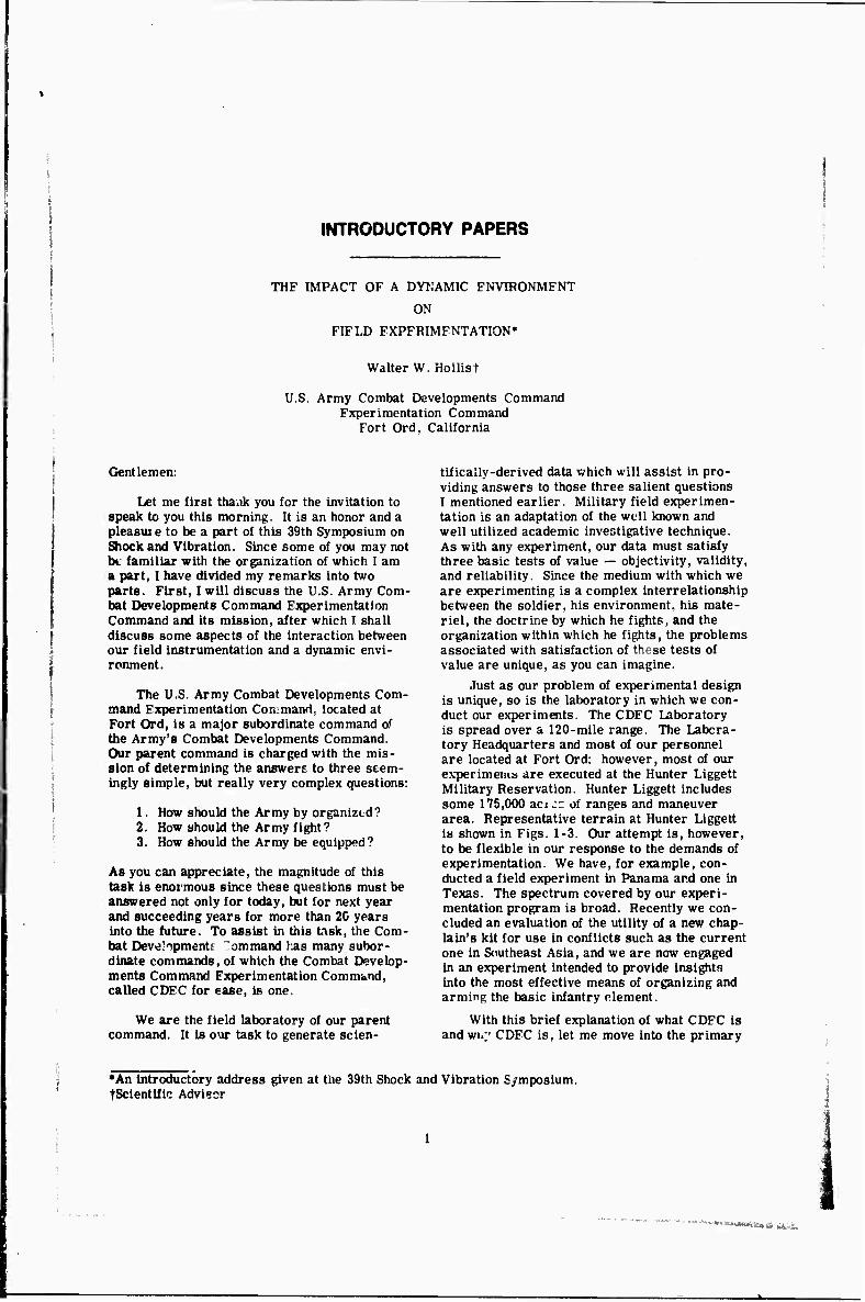
Those responsible for this task at CDEC, our Instrumentation Support Group, have been quite successful. The unit shown in Fig. 4 is the man portable responder unit which can both send and receive information pertinent to player activity. This unit is a part of a system by which a record of player position, event, occurrence, and time of event occurrence is maintained. One component of this unit, not shown in Fig. 4, is a probe which extends into the path of the muzzle blast, senses the firlag of a round and causes an appropriately coded signal to be transmitted by the transponder unit. I think all of you can appreciate the need for careful consideration of the dynamic environment in the design of such a device.

In the area of instrumentation for the individual soldier, we are now engaged in a development program for a direct fire weapon simulator. Fig. 5, which will permit us to con- dir * more realistic two-sided maneuvers than can be conducted at the present time. This device will be based upon the use of a pulse-coded gallium arsenide laser beam which will be used as the 'bullet' of the simulator. For realism, the soldier firing the simulator will simultaneously fire a blank cartridge from his weapon.

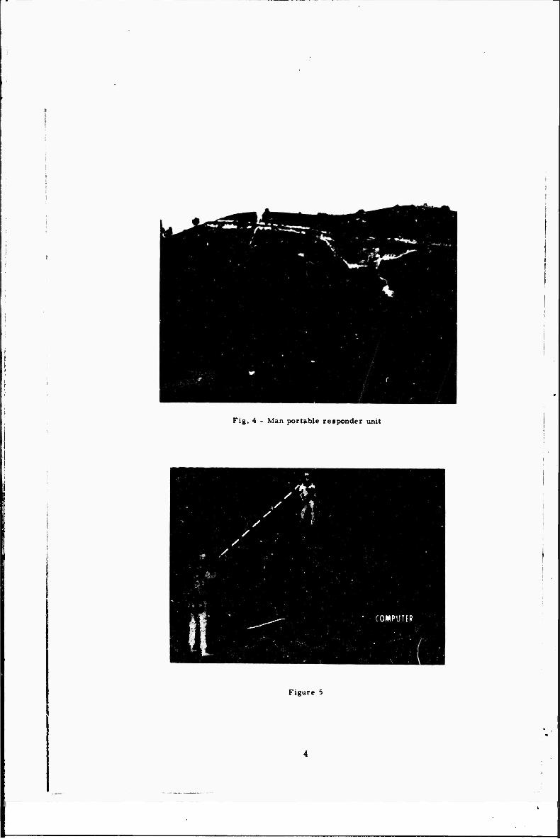
Fig. 4 - Man portable responder unit

1

i

1 - - •.

i

• COddPUTER

■ ■ 1 ■ . \ -.•■■:

Figure 5

<•

4

—

i

Fig. 6 - "Pop-up* personnel target

Hie recoil of the weapon and force of the hammer striking the firing pin cause vertical accelerations to the weapon which may cause the laser beam to miss the target since the logic of the simulator requires that three messages be transmitted by the weapon and received by the target in order to register a hit. The problem here, of course, is to identify accurately the timing sequence of all the actions which cause the vertical accelerations, identify the amount of time during which the hammer is falling, and then transmit the necessary laser messages in that time interval.

In the second category, I mentioned one of our principal items d instrumentation in the ■pop-up^ personnel target, Fig. 6. This target is the target we now employ on our 'live fire* ranges. The target is Instrumented to record hits and/or near misses from rifle fire, machine gun fire, and from the shrapnel caused by the detonation of 40-mm grenades. The construction of this target system permits protection of most of the instrumentation within the coffin; however, the target itself is

aluminum and any vibration inducea in the target as a result of a projectile hit could cause the registration of ' xalst. hits." Study of this potential problem led to the overcoating of the forward side of the target with a cellular rubber which effectively iamps the induced vibration below a level to which the hit sensing mechanism Is sensitive.

In the same category of instrumentation a potentially more difficult problem to solve is associated with our requirement for a vehicular target system which will be representative of a so-calUd "hard target," that is. a tank or ar- mored personnel carrier. This vehicular "pop- up" target must be capable of withstanding the shock Impact resulting from a direct hit from a projectile fired by a tank in main armament, be capable of sustaining more than one hit without destruction, and, of course, be economical to acquire. Our preliminary investigation into this problem indicates that a target constructed of fluted cardboard may be the answer; however, this investigation Is far from complete as I speak to you today.

TRANSCRIPT OF PANEL DISCUSSION

ON PROPOSED USASI STANDARD ON METHODS FOR

ANALYSIS AND PRESENTATION OF SHOCK AND VIBRATION DATA

Julius S. Bendat Measurement Analysis Corporation

Los Angeles, California

and

Allen J. Curtis Hughes Aircraft Corporation

Culver City, California

DR. BENDAT

We want this panel discussion to be an informal, extemporaneous, and informative discussion about work that has been going on for the last six years. This is the first public presentation on the results of this particular S2 Standards Committee to document and recommend standard methods for analyzing and presenting shock and vibration data, based on current usage and current understanding of the activities and the developments in the field. This work started in 1962 and the first Chairman was Dr. Charles Crede from Cal Tech. Dr. Crede headed a committee of which Dr. Curtis, Dr. Rubin, myself and others were members. Unfortunately when Dr. Crede died some four years ago, the work was still in an early phase, so we continued, and I was asked to take over as Chairman.

Many other people assisted us who represented a cross section of different interest groups from Government and Industry in the U.S. As the writing proceeded, it was necessary to «end preliminary drafts to these people for their comments, criticism and suggestions. This work went quite slowly and its only been in the last two days that we can now finally state that our work is Just about over. There was a meeting of the full S2 Committee here in Asilomar on Tuesday afternoon and at that time the last material that had been submitted by this committee was approved, to be transmitted to the U.S.A. Standards Institute for final action and ultimate distribution as a USASI Standard.

I might mention that besides the

three of us who were going to give this presentation today (we're sorry that Dr. Rubin is unable to attend), other people who have been Involved reviewing and approving the work Include L. L. Beranek. S. Edelman, C. A. Oolueke, H. H. Himelblau, D. C. Kcmnard, D. ifuster, W. W. Mutch, M. L. Stoner, H. E. von Olerke, representing groups from the Department of Defense, the American Society of Mechanical Engi- neers, the Acoustical Society of America, National Bureau of Standards, Institute of Electrical-Electronic Engineers, Society of Automotive Engi- neers, Institute of Environmental Sciences, National Electric Manufac- turers Association, and so on.

Now, what has resulted from this effort is a Standard of some hg pages that Includes a definite statement of the purpose and scope, every word carefully chosen. There is a listing of some 50 symbols which are used repeatedly, "nils does not constitute standardization of the symbols, it Just means that we use them, we recom- ment them, others are using them. This list doesn't replace the use of other symbols found elsewhere in some other Standard or in some other work. Also, there is a list of some hundred definitions of different terminology that appears throughout the literature and a great deal of current work. This includes definitions of some terms which have appeared in previous Stand- ards, so that we merely followed previous work; other definitions have had to be written for the first time. These are in alphabetical order and go all the way from "acceleration" through many of the terms that we will mention later this r,.omlng up to the last term

1

of Weakly Self Stationary Data," Some of these may be new to certain people here but they have become well enough understood now to be incorporated In such a Standard.

We also have a fairly comprehen- sive block diagram of recommended datix analyses and presentations - sort of overall considerations that you should have in mind regardless of your application. This has been distributed to each of you here for reference (see slides). It doesn't necessarily mean that you will follow every block in the diagram, but you should be aware of them and should use those that are pertinent to a particular application. This is one of some twenty diagrams in the Standard. The other diagrams in the Standard give greater details for individual blocks, different ways to compute certain of the functions or ways in which to display the results.

There is no attempt in this Standard to restrict anyone in the use of any particular equipment, analog, hybrid or digital, or to use any special computer data analysis program. There is no attempt to state specifically what parameters you should choose; these matters have to be determined as a result of a great deal of other work that would go along with these ideas. There are some references given to pertinent literature, and there is a great deal of emphasis on requirements that you should keep in mind.

These particular types of analyses and presentations are the ones that we consider fairly basic, fairly standard, and we feel there is no reason any more for people to be using these concepts in different ways. Confusion exists when the same term has a different interpretation on the part of different people. There were a number of points of view that had to be considered in this Standard and we tried as hard as we could to reconcile the various groups. Different peop.\e, of course, you know, have different needs and it is quite difficult as we learned over a four year history to get the agreement that we finally did achieve, so we are very pleased at the acceptance that has been obtained.

I want to emphasize again the fact that this Standard contains a number of very basic analysis procedures and basic data presentaticr. methods. Deviations are going to occur and will legitimately occur for many special applications, but I think

the requirement on people in the future who deviate from some of these recommendations will be that they must Justify their deviations. It is not a wholesome situation anymore when people are computing, for example, correlation functions or spectral density functions by a number of different methods without taking into consideration some of the basic requirements to make sure that other people who will examine their work cam properly interpret it. The analysis must be conducted in an accepted fashion and enough parameters must be made available to the analyst so he can do some appropriate error analysis for the displayed results if he so desires. Error analysis considerations are implied in the Standard. However, the exact procedures for carrying out error analysis were not in a state where they could be standardized as such.

The document, I think, will strike a very responsive chord in the mind of many people who have long felt a need for this material. It's our hope that as it becomes circulated, it will facilitate the application of these techniques to not only problems in shock and vibration but in many other fields as well. As a matter of fact, although there are many terms here that are restricted to shock and vibration, the actual scope of the Standard is broader, and would refer to random data regardless of the field in which it's obtained. I might briefly read a few words that state the purpose and scope of this document.

PURPOSE

"This Standard is designed to acquaint the user with general principles of the analysis and presentation of shock and vibration data, and to describe concisely several methods of reducing data to forms that can be applied and used in subsequent analyses. The Standard Includes references to the technical literature xor eluci- dation of applicable mathematical principles or where ready explanations are not available in the litftrature, an outline of applicable principles."

SCOPE

"T.iis Standard coven? vibration in the following idealized classes which are defined in Section 2.2. a. periodic vibration, b. aperiodic vibration, c, random vibration, and d. transient vibration (including shock). It is assumed that the data are available as time-histories of a variable

associated with shock and vibration, for example, acceleration, velocity, force, and ao forth and that any distortion resulting from the transducer, recording system, etc., has been eliminated. It Is recognized that In many Instances the vibration does not conform to this classification but rather consists of combinations of two or more classes. Suggestions are given for separating classe" as a necessary step in data analysis."

The purpose, the scope, and other details in the Standard represent the results on which we were able to obtain this general agreement that I mentioned. How Dr. Curtis or myself might apply some of these ideas, or how some of you might apply these ideas might be worthwhile additions, but they were not in a form, in a general enough way to be Included in the Standard. I think, in our later discussion, we will have to be very careful to state what is in the Stand- ard, as opposed to other practices not in the Standard (that we are aware of) which are used by some people.

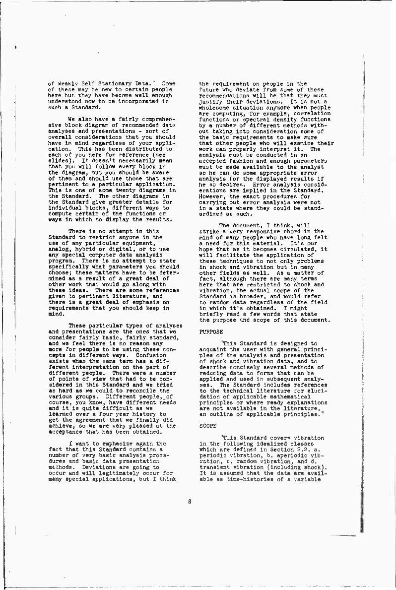
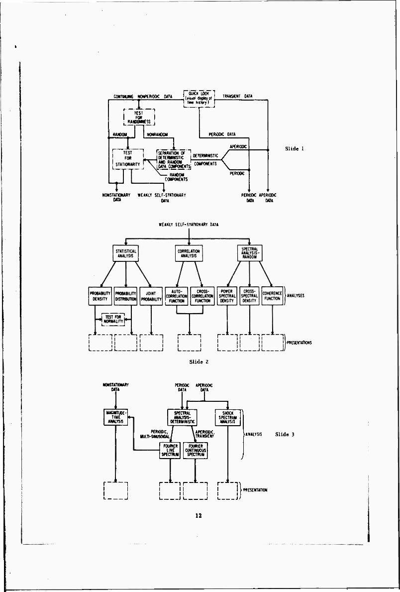
We have only three slides that we want to show and then we will open up the session to discussion. The three slides are a breakdown of the figure which has been passed out to you. You will note that there are, first of all, many steps involving classification and data qualification prior to the time that you actually do any specific analysis. TT^en there are six blocks across of different types of analysis. I would like to start out by discussing the initial preparation and classification of data, and then Dr. Curtis will go into some details of specific types of analysis and presentations.

SLIDE NO. 1

You will note that we start out with some time-history. The word time- history is descriptive only. You may prefer to call it the vibration, record, waveform or signal, it really doesn't matter. I think time-history is used by enough people, and we understand that it is some indication of behavior of the particular phenomena in question. It's a function of an independent variable which may be time or any other variable which can take the place of time. Our Job Is to analyze in as much detail as is needed for a particular application, the amplitude properties, frequency properties, and time related properties as might be contained in the data.

■friere are many extensions of ideas that are not In the Standard - we are very careful to restrict ourselves in the Standard to analysis of either Individual records or to pairs of records. You may want to get more information about an individual record as a result of being able to duplicate the analysis on similar results from other experiments. There is some discussion here of Joint statistical properties such as cross-correlation and cross-spectral density analysis, but we don't go into discussion of transfer functions or frequency response functions which represent important applications that you might want to make of spectral or cross- spectral results.

In the first part of the Standard, the top part of this diagram, you will note that the data needs to be separated out into three main types. The first type of data is transient, which means that its properties will die down. Next is periodic data, as defined classically, which goes on forever. Third is data which visually at least may not appear to be periodic or transient, &o it needs to be studied further. We call this third type continuing non-periodic data.

There are three special test blocks that may be required, but the actual procedure for carrying out the test for randomness, or the i«8t for stationarlty, or the test for normality, are not in the Standard. There are different ways that people are currently using for these tests and we didn't feel it appropriate at this stage of the game to standardize any of these tests. We merely wanted to indicate hers that there Is a need for such teats. It is necessary, in general, to qualify the data before you can do the later analysis to be sure that you are analyzing what you think you are analyzing.

A test for randomness is to separate out the random from the non- random components in the continuing nonperiodic data. It might be ignored by some trained analysts, but this omission is seldom recommended. It doesn't have to be a statistical test. It can be a practical test, fairly elementary. The actual ways in which you might carry out the test for randomness are not a part of the standard.

Itie most Important test requirement is probably the test for stationarlty. Again this test Is not In a

form that can be standardized, but here we definitely want to separate out non-stationary components from stationary components. All of these terms are defined in the StandarJ and we don't have time here to give a course or to go into these matters. I hope it will still be clear what's involved in our discussion. If the data is non-stationary, it must be analyzed by special methods which would be peculiar to the particular type of non-statlonarity. One such method which we felt Is in pretty good shape has been Included in the Standard, namely, a magnitude-time analysis which Dr, Curtis will discuss. There are many other procedures for analyzing non-stationary data - which are not in the Standard - that should be used where appropriate in current work. If the data does pass the test for stationarity, considering a single record, we really have the idea of weakly self- stationary data in mind. For usual cases of self-stationär!ty, this means that we are considering only the statlonarity of this one record rather than the stationarlty of a collection of records.

For weakly self-stationary data, there are certain types of accepted well-known analyses that have been in the field now for many years: statistical analysis, correlation analysis, spectral analysis. Basic results for these types of analyses are described in the Standard, the definitions of various terms, typical displays; results that we feel are so well established that there is a requirement on the part of everybody concerned to use these methods. Where you might go further into applications of these particular results, or in developing other special functions, you would be doing your own individual creative work.

Periodic data is deterministic data for which fairly classical well- known procedures are available, since there are explicit mathematical for- mulas to describe the properties, as opposed to random data which must be handled by probability or statistical techniques. Some of these accepted recognized procedures are in the Standard for analyzing periodic data. Finally, the analysis and presentation of transient data, also aperiodic data and shock data, can be standardized by means of Fourier or shock spectrum analysis techniques which are widely used, as discussed in the Standard.

The first discussion, and the first emphasis on data classification.

Is really the guideline for overall conslderstlons. After applying needed tests, as you perform the subsequent analysis, we point out in the Standard the Importance of keeping track of various parameters, so that somebody that follows you who wants to do some further detailed error analysis of a statistical sort would have the necessary parameters. I would like to turn over the discussion now to Dr. Curtis who will go into some of the detailed analysis and presentation recommendations.

DR. CURTIS

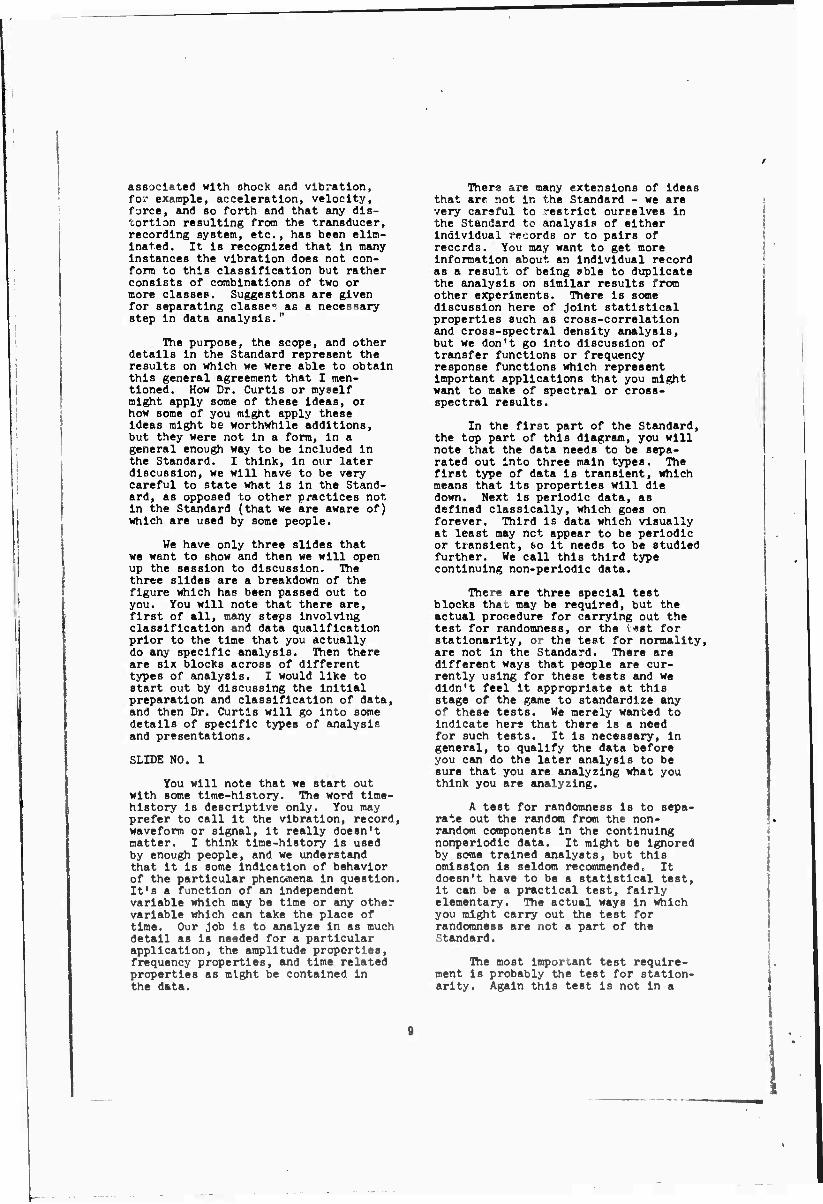
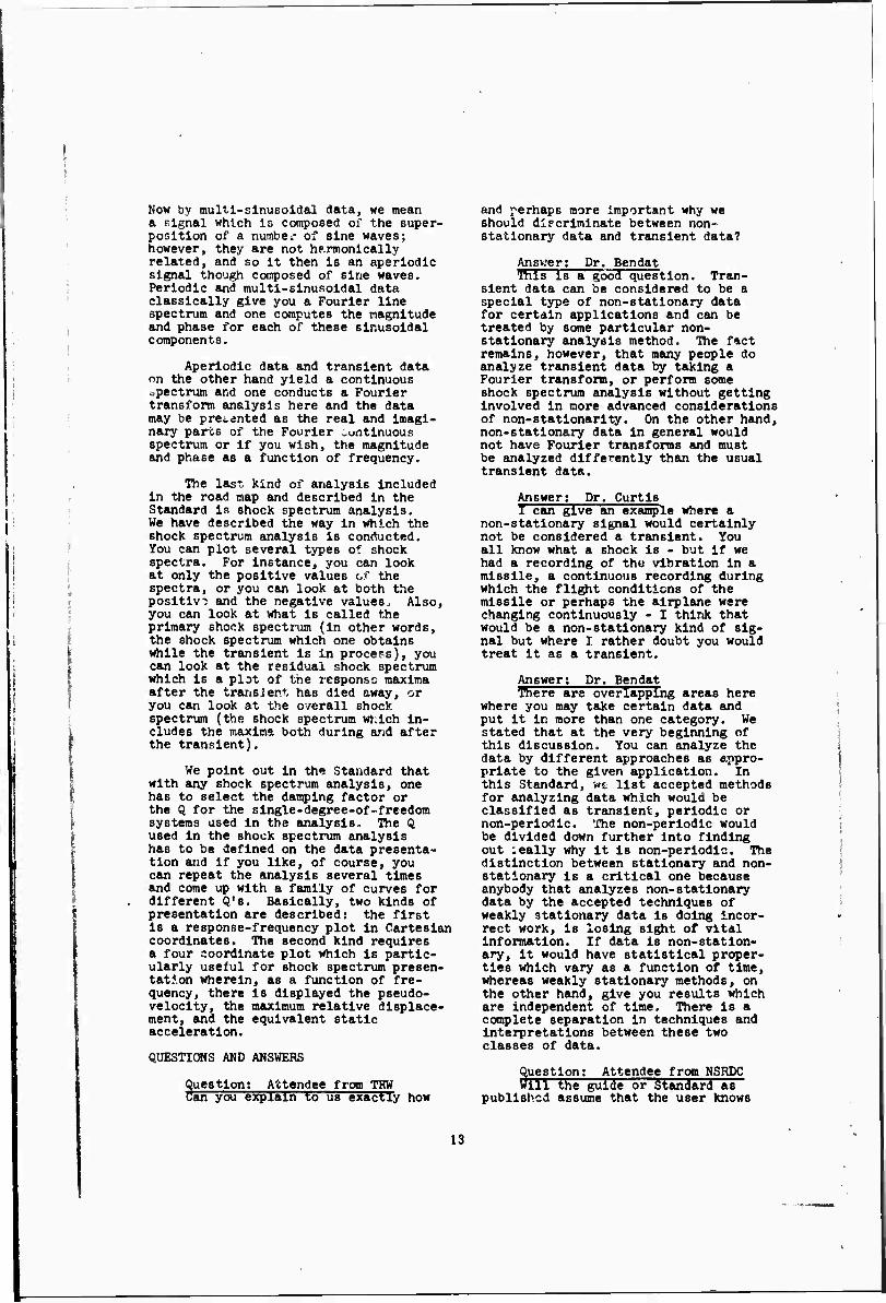
SLIDE NO. 2

This slide again Is Just a certain part of the road map, if you will, that we handed out to you and Includes all the blocks under weakly self- stationary data. It says that you've gone through this classification process, you've determined that it is weakly self-stationary data, and under here we try to indicate the kinds of analyses that can, possibly should, be done. Now you can separate these into three major kinds: statistical analysis, correlation analysis, and spectral analysis. Now these three are Interrelated, as I am sure you are aware, sir •> the performance of correlation analysis gives you some indication of the statistical characteristics of the signal and so in effect helps you In the statistical analysis. Likewise, for stationary data, it's possible to derive the spectral density plot from an auto- correlation analysis, and so they are again interrelated.

Under each of these three major classifications we indicate again sub-classifications of data analysis and the last line then describes the ways in which data after it has been analyzed in the prescribed way, should be presented. Now, we have not suggested what coordinate scales you should use or even particularly what physical units you should use, but we have indicated the kinds of units you should use. More particularly, we have said and we hope through this document that we can help standardize the Information which is Included on a particular data plot. For example, an incomplete spectral density plot is one that does not give you some Information about the bandwidth used for analysis, that does not tell you the length of the d&ta sample, or if you used a sweep filter, for instance, that does not define the sweep rate n* the filter. We have indicated throughout

10

the Standard the requirements for complete data presentation so that somebody else cap interpret what you did. Presumably If you do analysis. It's for understanding not only by yourself, but somebody else as well.

Under statistical analysis, we describe the principles, or some principles by which, this may be conducted. These principles apply equally well whether you are interested in the statistical nature of the instantaneous value of this time history, or the peak or maxima of the time-history. You can do this in two ways: you can look at the probability density of the signal which, for example, says what percentage of the time is the signal within a certain magnitude window, or you can look at the probability distribution which says what percentage of the time does the signal exceed a certain value. As I am sure you will remember, the probability distribution can be obtained as the integral of the probability density. When you have conducted such an analysis, then we indicate that probably a desirable analysis to perform is to compare the probability density or the distribution to the normal distribution to indeed check that you have a Gaussian distribution or how far you've strayed from that.

The third block Is a little more exotic, the joint probability analysis, where you take two signals and you are computing their Joint statistical or common statistical properties. The data presentation here, of course, becomes a three dimensional plot which is a little more difficult, but the Standard does Indicate what is necessary to do.

The correlation analysis breaks down into two types. First, autocorrelation, where one looks at the relationship for a single record between the values that it obtains a certain time Interval apart as one varies that time interval. Whereas, for cross- correlation, you have two signals and you are looking for the relationship as a function of a time shift, between the values of those two signals.

Spectral analysis breaks down into two kinds of analyses and a third one which is sort of a product of the other two. V.e have a power spectral density function shown as the first analysis. The word power, of course, can sometimes be questioned. It is perhaps a matter of personal taste and there is some thought that perhaps we should make thlf more syrametrical by calling it autospectral analysis. We

don't require this in the Standard but autocpectral denclty analysis is related to the autocorrelation function analysis, and here we are looking to find out what are the frequency characteristics of the signal. In cross- spectral analysis, it's a similar type except we have two records and we want to look at the frequency characteristics of these two signals simultaneously, and this kind of analysis is closely related to cross-correlation analysis. In other words, for correlation analysis you do things in the time domain whereas for spectral density analysis you do things in the frequency domain.

Coherence function, which may not be familiar to all of you. Is a function of frequency which Is numerically the ratio of the square of the magnitude of the cross-spectral density to the product of the autospectral densities (or power-spectral densities) of the individual signals. In all cases, we have indicated how ycu ought to present these kinds of data after you have conducted the analyses shown In the middle row.

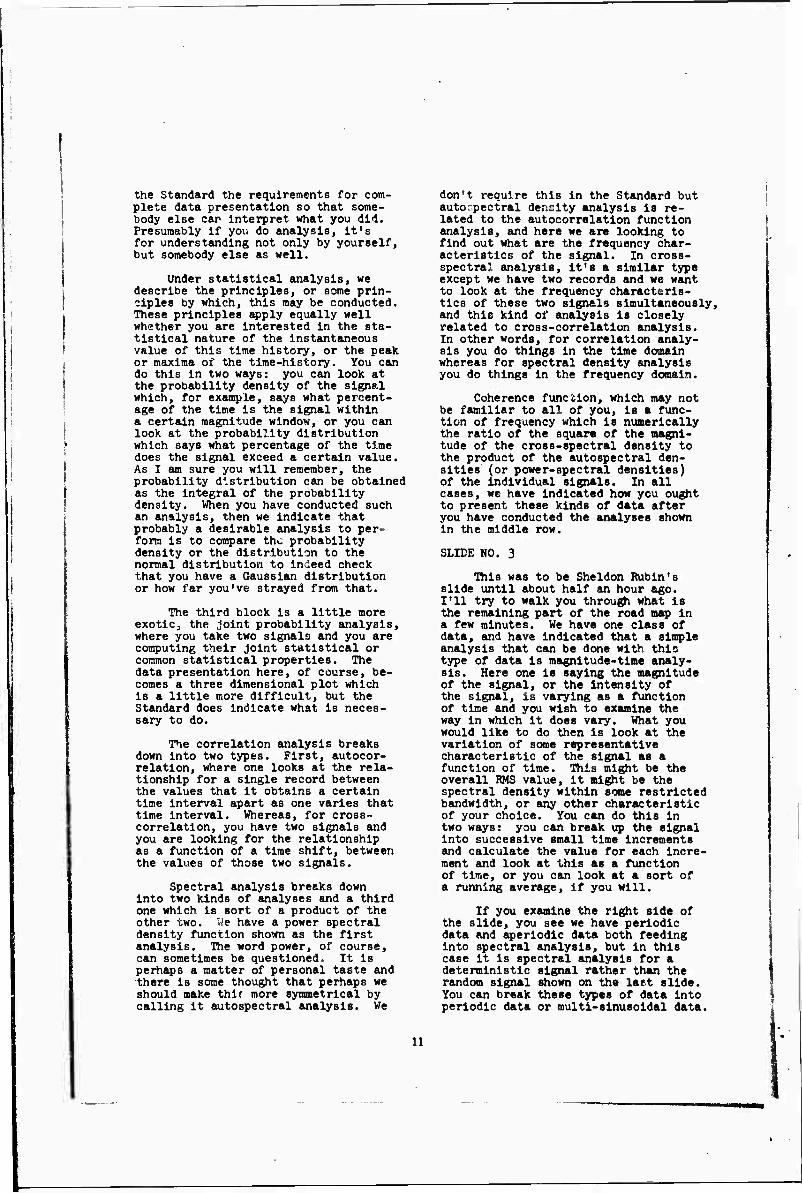
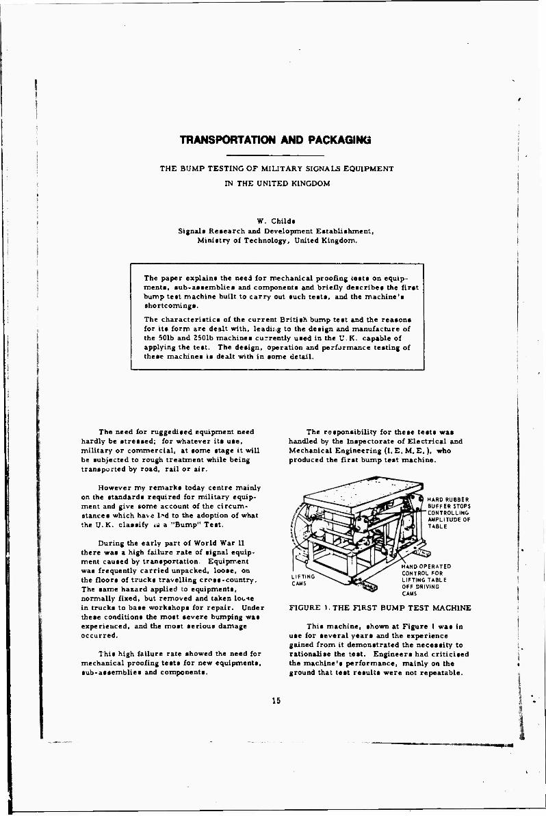
SLIDE NO. 3

This was to be Sheldon Rubin's slide until about half an hour ago. I'll try to walk you through what is the remaining part of the road map in a few minutes. We have one class of data, and have indicated that a simple analysis that can be done with this type of data is magnitude-time analysis. Here one is saying the magnitude of the signal, or the intensity of the signal, is varying as a function of time and you wish to examine the way in which it does vary. What you would like to do then is look at the variation of some representative characteristic of the signal as a function of time. This might be the overall RMS value, it might be the spectral density within some restricted bandwidth, or any other characteristic of your choice. You can do this in two ways: you can break up the signal Into successive small time increments and calculate the value for each incre- ment and look at this as a function of time, or you can look at a sort of a running average, if you will.

If you examine the right side of the slide, you see we have periodic data and aperiodic data both feeding into spectral analysis, but in this case it is spectral analysis for a deterministic signal rather than the random signal shown on the last slide. You can break these types of data into periodic data or multi-sinusoidal data.

11

CONTINUMC NOWtRiOOK MTA

i TEST . FOR RANOOMNCSS j

I tlM »III«J I I

RMCOH NONRANOOM

i ■ 1 r 1 1 1 «f OAOATIAU DC ■

PERIOUC DATA

«TERKNISTIC I OtTERWMSTIC AND RANDOM ' rnHPONENTS

JW^COII'OHENTSi ('w*wt"l:,

RANDOM COMPONENTS

NONSTATKMARY WEAKLY SELF-STATIONARY M» OATA

AKRIOOC

PERSOOtC

Slide 1

PERNOK APERIODIC DATA DATA

WEAKLY SELF-STATIONARY DATA

ANALYSES

PRESENTATIONS

Slide 2

NONSTATIONARY DATA

MAGNfTUOE TIME

ANALYSIS h

PCRIOOK DATA

APERiODK

SPECTRAL ANALYSI5-

DETERMINISnC

PERIODIC, MULTI-SINUSOIDAL

I

a SHOCK

SPECTRUM ANALYSIS

APERIODIC, TRANSIENT

FOURIER LINE

SPECTRUM

FOURIER CONTINUOUS

SPECTRUM

I

i r- II I I I I

J I 1

._Jl_

'ANALYSIS Slide 3

i I I PRESENTATION 1 'I I J/

12

Now by multi-sinusoidal data, we mean a signal which Is composed of the super- position of a number of sine waves; however, they are not hP.rmonlcally related, and so it then is an aperiodic signal though composed of sine waves. Periodic and multi-slnusoldal data classically give you a Fourier line spectrum and one computes the magnitude and phase for each of these sinusoidal components.

Aperiodic data and on the other hand yield spectrum and one conduct transform analysis here may be presented as the nary parts of the Fourie spectrum or if you wish, and phase as a function

transient data a continuous s a Fourier and the data real and imagi- r iuntlnuous the magnitude

of frequency.

The last kind of analysis included in the road map and described in the Standard is shock spectrum analysis. We have described the way In which the shock spectrum analysis is conducted. You can plot several types of shock spectra. For instance, you can look at only the positive values of the spectra, or you can look at both the positiv: and the negative values. Also, you can look at what Is called the primary shock spectrum (in other words, the shock spectrum which one obtains while the transient is in process), you can look at the residual shock spectrum which is a plat of the response maxima after the transient has died away, or you can look at the overall shock spectrum (the shock spectrum which includes the maxima both during and after the transient).

We point out in the Standard that with any shock spectrum analysis, one has to select the damping factor or the Q for the slngle-degree-of-freedom systems used In the analysis. The Q used In the shock spectrum analysis has to be defined on the data presentation and If you like, of course, you can repeat the analysis several times and come up with a family of curves for different Q's. Basically, two kinds of presentation are described: the first is a response-frequency plot in Cartesian coordinates. The second kind requires a four coordinate plot which Is particularly useful for shock spectrum presentation wherein, as a function of frequency, there is displayed the pseudo- velocity, the maximum relative displacement, and the equivalent static acceleration.

QUESTIONS AMD ANSWERS

juestlon; Attendee from TRW ^an you explain to us exactly how

13

and perhaps more Important why we should dlecriminate between non- stationary data and transient data?

Answer; Dr. Bendat This is a good question. Tran-

sient data can be considered to be a special type of non-stationary data for certain applications and can be treated by some particular non- stationary analysis method. The fact remains, however, that many people do analyze transient data by taking a Fourier transform, or perform some shock spectrum analysis without getting Involved in more advanced considerations of non-stationarity. On the other hand, non-stationary data in general would not have Fourier transforms and must be analyzed differently than the usual transient data.

Answer; Dr. Curtis I can give an example where a

non-stationary signal would certainly not be considered a transient. You all know what a shock is - but If we had a recording of the vibration in a missile, a continuous recording during which the flight conditions of the missile or perhaps the airplane were changing continuously - I think that would be a non-stationary kind of signal but where I rather doubt you would treat it as a transient.

Answer; Dr. Bendat There are overlapping areas here

where you may take certain data and put it in more than one category. We stated that at the very beginning of this discussion. You can analyze the data by different approaches as Appro- priate to the given application. In this Standard, v»t list accepted methods for analyzing data which would be classified as transient, periodic or non-periodic. The non-periodic would be divided down further Into finding out :eally why it is non-periodic. The distinction between stationary and non- stationary is a critical one because anybody that analyzes non-stationary data by the accepted techniques of weakly stationary data is doing incorrect work, is losing sight of vital information. If data is non-stationary, it would have statistical properties which vary as a function of time, whereas weakly stationary methods, on the other hand, give you results which are independent of time. There is a complete separation In techniques and interpretations between these two classes of data.

Question; Attendee from NSRDC Will the guide or Standard as

published assume that the user knows

why he will use this Stand«;rd or do you provide guidance and examples of why you would do certain types of analysis in order to get certain types of presentations?

Answer; Dr. Bendat The Standard does not replac the

need for understanding basic concepts or practical Knowledge on the part of the user. It is very restricted In scope. The user must supply his own Justification for why he wants to do any part of the analysis that he might conduct. Application areas as such are not included in the Standard.

This Standard can be used for many different application areas. I Know of other worK going on in Oceanography, Communications, Seismology, etc., which also require the same ideas that are included in the Standard. I think that it would be very difficult, if not impossible, to get agreement on these matters from as many people who have been Involved in this over the past six years if we tried to standardize particular applications or particular interpretations. I am amazed and really very pleased at the final results of this sustained effort, that we were able to get agreement on what is contained in the Standard. There are many guidelines here, many valuable ideas, and many things are implied besides what is actually stated in the Standard, but what is stated is very specific on recommended ways in which to use certain terms and the recommended ways to canv out certain analyses, listing important parameters and displaying results.

Question; Attendee from Aerospace Corporation

Tht Joint probability distribution that is Included, is it for two signals or for more than two signals?

Answer; Dr. Curtis You asked if the Joint probability

was for mor^ than two signals. The material in the Standard restricts itself to how to compute the Joint probability distribution for two signals only. It does not explore the more general case.

America Standards Institute for their final action and distribution. I don't know how fast they are able to move. We ourselves are now essentially through with our contributions and expect to send this material to the Standards Institute within the next thirty days. Those of you that may be interested in getting a copy because of your current work can obtain one by writing to me in Los Angeles.

There is a lot of room that's still left in this field in the way of future Standards and future applications. There are many challenges and opportunities for different people who have different facilities who will actually carry out the work. There is no restriction in this Standard at all - as we said - on the use of any particular instruments or any particular digital computer programs. However, if you want to have a compre- hensive capability, then clearly we have stated here at least the minimum requirements that should be available to you. Which particular types of analyses you would conduct will vary considerably from user to user. No- body in his right mind should ever take any raw data and go through and compute all of these functions. It would be a waste of a great deal of effort. On the other hand, if you only collect data and Immediately do a power spectral density analysis, that would also be wrong because nobody covld interpret the results. You must qualify data along the way to make sure that any particular analysis is appropriate to that particular data for some specific application.

On this positive note, the session is adjourned.

Qu« m Question len do you hope to have this

Standard in effect?

Answer; Dr. Bendat well, as I mentioned, two days

ago we received approval here from the S2 Committee on our last draft of the Standard, and were authorized to submit it to the United States of

14

TRANSPORTATION AND PACKAGING

THE BUMP TESTING OF MILITARY SIGNALS EQUIPMENT

IN THE UNITED KINGDOM

W. Child« Signalt Research and Development Eitabliihment,

Miniitry of Technology, United Kingdom.

The paper explain« the need for mechanical proofing tests on equipment«, sub-aiiemblie« and component« and briefly describe« the fir«t bump test machine built to carry out «uch te«t«, and the machine1« shortcoming«.

The characteristics of the current British bump test and the reasons for it« form are dealt with, leadii.g to the design and manufacture of the 501b and 2501b machine« currently used in the U.K. capable of applying the test. The design, operation and performance testing of these machines is dealt with in some detail.

The need for ruggedised equipment need hardly be stressed; for whatever its use, military or commercial, at some «tage it will be «ubjected to rough treatment while being transported by road, rail or air.

However my remark« today centre mainly on the standard« required for military equipment and give tome account of the circum- stance« which have l->d to the adoption of what the U.K. cla««ify is a "Bump" Test.

During the early part of World War II there was a high failure rate of signal equipment cau«ed by transportation Equipment was frequently carried unpacked, loose, on the floor« of truck« travelling cross-country. The same hazard applied to equipments, normally fixed, but removed and taken locie in trucks to base workshops for repair. Under these conditions the most severe bumping was experienced, and the most «erioue damage occurred.

This high failure rate «howed the need for mechanical proofing testa for new equipment«, sub-assemblies and components.

The responsibility for these test« wa« handled by the Inspectorate of Electrical and Mechanical Engineering (I. E. M. E,), who produced the first bump test machine.

HARD RUBBER BUFFER STOPS CONTROLLING AMPLITUDE OF TABLE

HAND OPERATED CONTROL FOR LIFTING TABLE OFF DRIVING CAMS

FIGURE I. THE FIRST BUMP TEST MACHINE

This machine, shown at Figure 1 was in use for several year« and the experience gained from it demonstrated the neceaaity to rationaliae the teat. Engineera had criticiaed the machine'a performance, mainly on the ground that teat results were not repeatable.

15

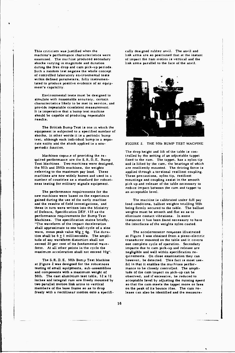
This criticism was justified when the machine's performance characteristics were examined. The machine produced secondary shocks varying in magnitude and duration during the free drop and cam pick-up periods. Such a random test negates the whole concept of controlled laboratory environmental tests within defined parameters, fully instrumen- tated to produce positive evidence of an equipment's capability.

Environmental tests must be designed to simulate with reasonable accuracy, certain characteristics likely to be met in service, and provide repeatable cc isistent measurement. It is imperative that a bump test machine should be capable of producing repeatable results.

The British Bump Test is one in which the equipment is subjected to a specified number of shocks, in other words it is a periodic bump test, although each individual bump is a separate entity and the shock applied is a non- periodic function.

Machines cap.Ho.e of providing the required performance are the S. R. D. E, Bump Test Machines. Two machines were designed, the 501b and 2501b machines, the weights referring to the maximum pay load. These machines are now widely known and used in a number of countries as a standard for robustness testing for military signals equipment.

The performance requirements for the new machines were based on the experience gained during the use of the early machine and the results of field investigations, and these in turn were written into the Ministry of Defence, Specification DEF. 133 as the performance requirements for Bump Test Machines. The specification states briefly, "The waveform of the impact deceleration shall approximate to one half-cycle of a sine wave, mean peak value 40g + 4g. The duration shall be 6 + 1 milliseconds. The amplitude of any waveform distortion shall not exceed 20 per cent of its fundamental waveform. At all other points in the cycle the maximum acceleration shall not exceed 10g".

The S. R. D. E. 501b Bump Test Machine at Figure 2 was designed for the robustness testing of small equipments, sub-assemblies and components with a maximum weight of 501b. The cast aluminium test table, 12 x 12 inches and integral ram are freely mounted by two parallel motion link arms to vertical members of the base frame so as to drop freely with a rectilinear motion onto a specifi-

cally designed rubber anvil. The anvil and link arms are so positioned that at the instant of impact the ram motion is vertical and the link arms parallel to the face of the anvil.

FIGURE 2. THE 501b BUMP TEST MACHINE

The drop height and lift of the table is controlled by the setting of an adjustable tappet fixed to the ram. The tappet, has a nylon tip and is lifted by the cam, the bearings of which are resiliently mounted. The driving force is applied through a torsional resilient coupling. These precautions, nylon tip, resilient mountings and coupling assist in the smooth pick up and release of the table necessary to reduce impact between the cam and tappet to an acceptable level.

The machine is calibrated under full pay load conditions, ballast weights totalling 501b being firmly secured to the table. The ballast weights must be smooth and flat so as to eliminate contact vibrations. In some instances it has been found necessary to have the interfaces of the weights nylon coated.

The accelerometsr response illustrated at Figure 3 was obtained from a piezo-electric transducer mounted on the table and it covers one complete cycle of operation. Secondary impacts due to cam pick-up and release are negligible and well within specification requirements. On close examination they can however, be detected. This fact is most useful in that it enables the machines performance to be closely controlled. The amplitude of the cam impact on pick-up can be observed, and if excessive, be reduced to acceptable level by adjusting the running speed so that the cam meets the tappet more or less on the peak of its bounce rise. The cam release can also be identified and the measure-

16

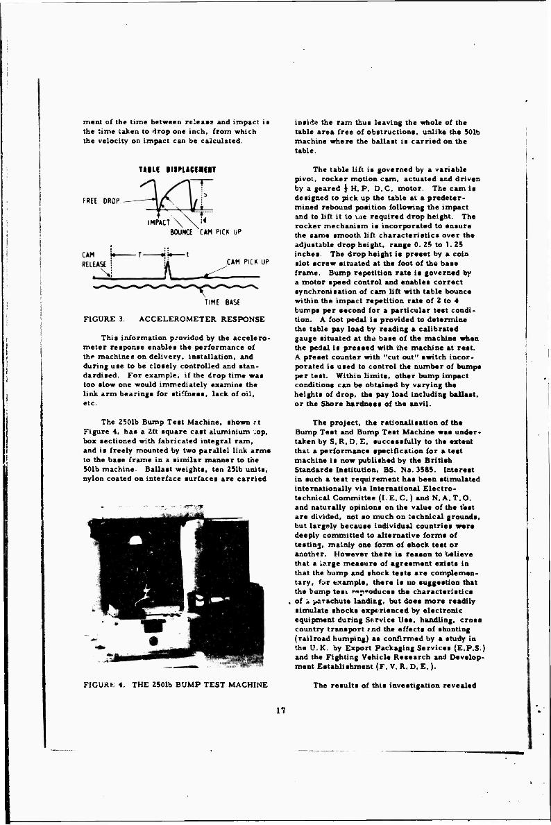
ment of the time between releate and impact ii the time taken to drop one inch, from which the velocity on impact can be calculated.

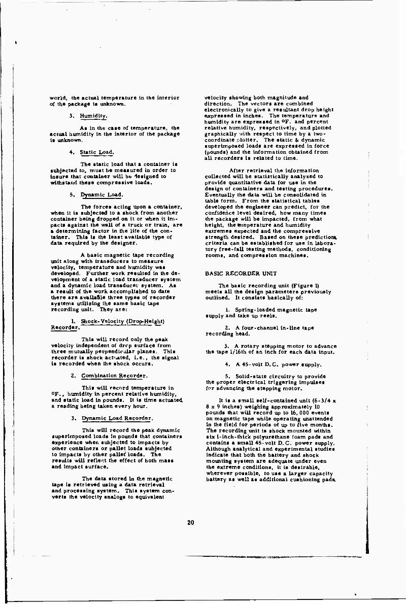
inairie the ram thui leaving the whole of the table area free of obitructiona, unlike the 501b machine where the ballaat it carried on the table.

Ulli •lin<CE«HT

FREE DROP

IMPACT x \ :* BOOMtt CAM PICK UP

CAM PICK UP

TIME BASE

FIGURE 3. ACCELEROMETER RESPONSE

Thit information p/ovidcd by the accelerometer reiponae enables the performance of the machine« on delivery, initallation, and during uie to be closely controlled and »tan- dardiaed. For example, if the drop time wa* too slow one would immediately examine the link arm bearing« for «tiffne««, lack of oil, etc.

The table lift is governed by a variable pivot, rocker motion cam, actuated and driven by a geared | H. P. D. C. motor. The cam i« designed to pick up the table at a predetermined rebound position following the impact and to lift it to lae required drop height. The rocker mechanism i« incorporated to ensure the same smooth lift characteristics over the adjustable drop height, range 0. 25 to 1. 25 inches. The drop height is preset by a coin slot screw situated at the foot of the base frame. Bump repetition rate is governed by a motor speed control and enables correct synchronisation of cam lift with table bounce within the impact repetition rate of 2 to 4 bumps per second for a particular test condition. A foot pedal is provided to determine the table pay load by reading a calibrated gauge situated at th« base of the machine when the pedal is pressed with the machine at rest. A preset counter with "cut out" switch incorporated is used to control the number of bumps per test. Within limits, other bump impact conditions can be obtained by varying the heights of drop, the pay load including ballast, or the Shore hardness of the anvil.

The 2501b Bump Test Machine, shown ;t Figure 4, has a 2ft square cast aluminium .op, box sectioned with fabricated integral ram, and is freely mounted by two parallel link arms to the base frame in a similar manner to the 501b machine. Ballast weights, ten 251b units, nylon coated on interface surfaces are carried

.Tr-;-T»

FIGURt 4. THE 2501b BUMP TEST MACHINE

The project, the rationalisation of the Bump Test and Bump Test Machine was undertaken by S. R. D. E. successfully to the extant that a performance specification for a test machine is now published by the British Standards Institution, BS. Na. 3585. Interest in such a test requirement has been stimulated internationally via International Electro- technical Committee (I. E. C.) and N. A. T. O. and naturally opinions on the value of the test are divided, not so much on technical grounds, but largely because individual countries were deeply committed to alternative forms of testing, mainly one form of shock test or another. However there is reason to believe that a Large measure of agreement exists in that the bump and shock tests are complemen- tary, tut example, there is uo suggestion that the bump tesi reproduces the characteristics of ä parachute landing, but does more readily simulate shocks experienced by electronic equipment during Service Use, handling, cross country transport «nd the effects of «hunting (railroad humping) as confirmed by a study in the U.K. by Export Packaging Services (E.P.S.) and the Fighting Vehicle Research and Develop- ment Establishment (F. V. R. D. E.).

The results of this investigation revealed

17

that loose piece» of equipment up to 100 lb in weight experience »hock levels of up to 100 g when traceposrted under hazardous condition*, aero»» rough country. Duration of »ignificant impact» range from 5 to 35 millieecond». The occurrence of bump» above the 40g level are relatively few and we conaider that these would be adequately covered by the Drop and Push- over Tests. By far the greater number of bumps experienced during these trials which covered several types of Army transport vehicles driven at various speeds over poor road, pave and rough cross country terrain were of the order of 40g and less. Thus it wo'-' ' appear that the choice of the 40g impact, duration 6 milliseconds, would be of sufficient severity for use as a standard for robustness testing. The results obtained from transport- ing a piece of equipment loose in a 3 ton truck over rough country are graphically illustrated in Figure 5.

ocmaoM m «oas swww KMCM. i MT iseutio Mocn or m*a» M-MC MWUTMC Mt Or i TO ».SKOt» WMTWI,

Many of you may feel concerned that the adoption of such a bump test universally might adversely effect the economics of equipment development. Experience in the U. K. has shown that this is not so, since, in fact, any equipment structure built on sound engineering principles will certainly survive the 40g condition. Any higher levels, for example 80g, would, we agree, result in a severe rise in development costs. It is interesting to nots that certain manufacturer», mainly of domeatic equipment have adopted a 20g teat. The number of bumps. 4,000 ha» been the ba»i» of an acceptable relationship between the life of the equipment and coat of con»truction - good engineering construction in relation to cost factor.

The Bump Test is included in all our environmental specifications for new equipments which are liable to be transported loosely and not permanently fixed in the vehicle. It is applied at temperature extremes -40oC and +50oC with solar radiation covering transport in open vehicles.

It is also used in an abbreviated form, 100 bumps, as a shake down test during factory inspection. This augments the re- moval of foreign matter, for example loose bit» of »older, nut» sind etc. , and help» to reveal faulty workmanship, dry »oldered connection», poor welding, loose nuts and bolts and badly mounted components. The production qualification tests are then applied and finally we should have a robust equipment capable of reliable performance in the field. This is the British Bump Test.

FIGURE 5. GRAPHIC REPRESENTATION OF SHOCK LEVELS MEASURED ON AN EQUIP- MENT TRANSPORTED LOOSE IN A 3-TON TRUCK OVER ROUGH TERRAIN.

British Crown copyright, reproduced with the permission of the Controller, Her Britannic Majesty's Stationery Office.

DISCUSSION

Mr. Swanson (MTS System» Corp.): Could you elaborate on the transverse bumping? For Instance, in service the radio looked as though It got a few sideways Jolts. How do you check nut the transverse effects ?

Mr. Chllds: You only saw part of the bump test. It Is applied In each of three planes. If

there are three planes on which it can stand, it gets 3000 bumps In each of those planes.

Mr. Swanson: All to the same g-level?

Mr. Chllds: Yes.

18

NLABS SHIPPING HAZARDS RECORDER STATUS A.ND FUTURE

PLANS

Denis J. O'SulUvan. Jr. S. Army Natick Laboraiorie«

Natick, Masiachuaetts

The paper describes the basic recorder unit developed by NLABS to measure the shipping hazards that packages encounter in worldwide distribution and storage. Also described are the transducers used with the basic recorder to measure velocity, temperature, humidity, static load, dynamic load and acceleration. The status of the program is presented along with future plans and the results of the limited test shipment.

INTRODUCTION

There is a continuing need within the Department of Defense for reliable information on conditions encountered by military supplies during worldwide distribution and storage. In 1955 an Ad Hoc Commit- tee was established to collect the information but was deactivated in 1963 due to the lack cf suitable recording instrumentation to measure the desired conditions. As a result today's packaging design engineer has to rely on "empirical and nebulous criteria" established through experience, to design elective packages. In most instances the packages have excellent protective qualities but are overpacked, resulting in excessive material and labor cost. In some instances they are underdesigned resulting in damaged contents.

About 5 years ago, in an attempt to provide the packaging engineer the necessary information, the U. S. Army Natick Laboratories established a design criteria program to devise the ways and means required to meas ire and record the shipping hazards encountered by military supplies during worldwide distribution and storage. A contract was awarded to determine the availability of suitable recording units that would meet the following requirements:

1. Be compact.

2. Have a large mwnory bank.

3. Be capable of long periods of unattended operation.

4. Be compatible with automatic data processing equipment.

5. Be able to distinguish clearly between each shock input.

6. Be able to distinguish between positive and negative shock inputs.

7. Have a time code.

The study showed that no commercial recorders were available and work was be- gun to develop a recorder to measure five parameters:

1. Shock (Drop-Height).

Venetos (1) has indicated that the greatest damage to a container is likely to occur when the container is dropped during a handling operation. Therefore, the packaging engineer must have available an expression of the magnitude of the shocks incurred by the container. It was determined that the measurement of velocity would be the most useful. Knowing the velocity, the impact energy which protective packaging must absorb can be calculated. Also, velocity can readily be converted to an equivalent drop height (V = VTgK—I) which can be directly related to many container testing procedures based on the free-fall impacting of containers.

2. Temperature.

While there is much data on the climatic conditions in various parts of the

19

I

world, the actual temperature in the Interior of the package It unknown.

3. Humidity.

Aa in the case of temperature, the actual humidity in the interior of the package la unknown.

4. SUtic Load.

The atatic load that a container it subjected to, must be measured in order to insure that container will be designed to withstand these compressive loads.

5. Dynamic Load.

The forces acting upon a container, when it is subjected to a shock from another container being dropped on it or when it impacts against the wall of a truck or train, are a determining factor in the life of the container. This is the least available type of data required by the designer.

A basic magnetic tape recording unit Along with transducers to measure velocity, temperature and humidity was developed. Further work resulted in the development of a static load transducer system and a dynamic load transducer system. As a result of the work accomplished to date there are availaBle three types of recorder systems utilizing the same basic tape recording unit. They are:

1. Shock-Velocity (Drop-Height) Recorder.

This will record only the peak velocity independent of drop surface from three mutually perpendicular planes. This recorder is shock actnated, i. e., the signal is recorded when the shock occurs.

2. Combination Recorder.

This will record temperature in 0F., humidity in percent relative humidity, and static load in pounds. It is time actuated a reading being taken every hour.

3. Dynamic Load Recorder.

This will record the peak dynamic superimposed loads in pounds that containers experience when subjected to impacts by other containers or pallet loads subjected to impacts by other pallet1 loads. The results will reflect the effect of both mass and impact surface.

The data stored in the magnetic tape is retrieved using a data retrieval and processing system. This system con- verts the velocity analogs to equivalent

velocity showing both magnitude and direction. The vector« are combined electronically to give a resultant drop height expressed in inches. The temperature and humidity are expressed in 0F. and percent relative humidity, respectively, and plotted graphically with respect to time by a two- coordinate plotter. The static 8c dynamic superimposed loads are expressed In force (pounds) and the Information obtained from all recorders Is related to time.

After retrieval the Information collected will be statistically analyzed to provide quantitative data for use In the design of containers and testing procedures. Eventually the data will be consolidated In table form. From the statistical tables developed the engineer can predict, for the confidence level desired, how many times the package will be Impacted, from what height, the temperature and humidity extremes expected and the compressive strength desired. Based on these predictions^ criteria can be established for use In laboratory free-fall testing methods, conditioning rooms, and compression machines.

BASIC RECORDER UNIT

The basic recording unit (Figure 1) meets all the design parameters previously outlined. It consists basically of:

1. Spring-loaded magnetic tape supply and take up reels.

Z. A four-channel In-line tape recording head.

3. A rotary stepping motor to advance the tape l/16th of an inch for each data input.

4. A 45-volt D. C. power supply.

5. Solid-state circuitry to provide the proper electrical triggering Impulses f<->r advancing the stepping motor.

It Is a small self-contained unit (6-3/4 x 8x9 Inches) weighing approximately 10 pounds that will record up to 16, 000 events on magnetic tape while operating unattended in the field for periods of up to five months. T^he recording unit is shock mounted within six 1-lnch-thick polyurethane foam pads and contains a small 45-volt D. C. power supply. Although analytical and experimental studies Indicate that both the battery and shock mounting system are adequate under even the extreme conditions, it is desirable, wherever possible, to use a larger capacity battery as well as additional cushioning pads.

20

Figure 1. Bailc Recording Unit

21

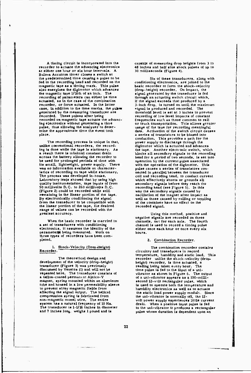
A timing circuit ic incorporated into the recorder to actuate the advancing electronics at either one hour or »ix hour intervale. A Bulova Accutron tinner closet a switch at the predetermined time causing a pulse to be fed to the recording head and recorded on the magnetic tape as a timing mark. This pulse aliio energises the dlgimotor which advances the magnetic tape l/16th of an inch. The recording of parameters can either be time actuated, as in the case of the combination recorder, or force actuated. In the latter case, la addition to the time marks, the pukes generated by the measuring transducer are recorded. These pulses after being recorded on magnetic tape actuate the advancing electronics without generating a time pulse, thus allowing the analyzer to determine the approximate time the «vent took place.

The recording process is unique in that, unlike conventional recorders, the recording is done while the tape is stationary. As a result there is minimal constant drain across the battery allowing the recorder to be used for prolonged periods of time with its small, lightweight, power supply. There was no information available on characteristics of recording on tape while stationary. The process was developed in-house. Laboratory tests showed that by using high quality instrumentation, tape inputs of from 50 millivolts D.C. to 260 millivolts D.C. (Figure 2) could be recorded while still remaining in the linear portion of the tape. By electronically conditioning the signal from the transducer to be compatible with the linear portion of the tape, the desired range of values can be recorded with the greatest accuracy.

When the basic recorder is married to a set of transducers with conditioning electronics, it assumes the identity of the parameter being measured. Work on three types of recorders have been completed.

1. Shock-Velocity (Drop-Height) Recorder,

The theoretical design and development of the velocity (drop-height) transducer (Figure 3) was previously discussed by Venetos (1) and will not be repeated here. The transducer consists of a teflon-coated permanent Alnico-V magnet, spring mounted within an aluminum tube and housed in a low permeability sleeve to prevent stray magnetic fields from affecting the signal output. The helical compression spring is fabricated from non-magnetic monel wire. The entire system has a natural frequency of 10 He. The transducer is 1-1/16 inches in diameter and 7 inches long, weighs 1 pound and is

capable of measuring drop heights from 3 to 48 inches and half sine shock pulse« of up to 30 milliseconds (Figure 4).

Six of these transducers, along with conditioning electronics, are joined to the basic recorder to form the shock-velocity (drop-height) recorder. On Impact, the signal generated by the transducer is fed through an actuating switch circuit which, if the signal exceeds that produced by a 3-inch drop, is turned on until the maximum «ignal is produced and recorded. The threshold level is set at 3 inches to prevent recording of low level impacts of constant frequencies such as those common to rail or truck transportation. This allows greater usage of the tape for recording meaningful data. Activation of the switch circuit causes a series of transistors to be biased Into conduction. This provides a path for the power supply to discharge through the dlgimotor which Is actuated and advances the tape. Another electronic switch, which blocks all secondary signals to the recording head for a period of two seconds, is set into operation by the current pulse associated with the operation of the dlgimotor. This pulse causes a series of transistors connected in parallel between the transducer coil and recording head, to conduct current which effectively shorts or grounds all secondary signals before they reach the recording head (see Figure 5). In this way the secondary signals caused by oscillation of the magnet after impact as well as those caused by rolling or toppling of the container have no effect on the recorded signal.

Using this method, positive and negative signals are recorded on three channels, ona for each axis. The fourth channel is used to record a timing pulse either once each hour or once every six hours.

2. Combination Recorder.

The combination recorder contains circuitry and transducers to record temperature, humidity and static load. This recorder unlike the shock-velocity (drop, height) recorder. Is time actuated, a reading being taken every hour. The time pulse Is fed to the Input of a Uni- vibrator as shown In Figure 6. The output of a uni-vibrator appears as a 100-mllll- second 12-volt rectangular pulse, which is used to operate both the temperature and humidity electronics as well as to actuate the static load power supply module. Since the uni-vibrator is normally off, ths 12- volt power supply experiences little current drain. When a positive Input pulse is fed to the uni-vibrator it produces a rectangular pulse whose duration is dependent upon an

22

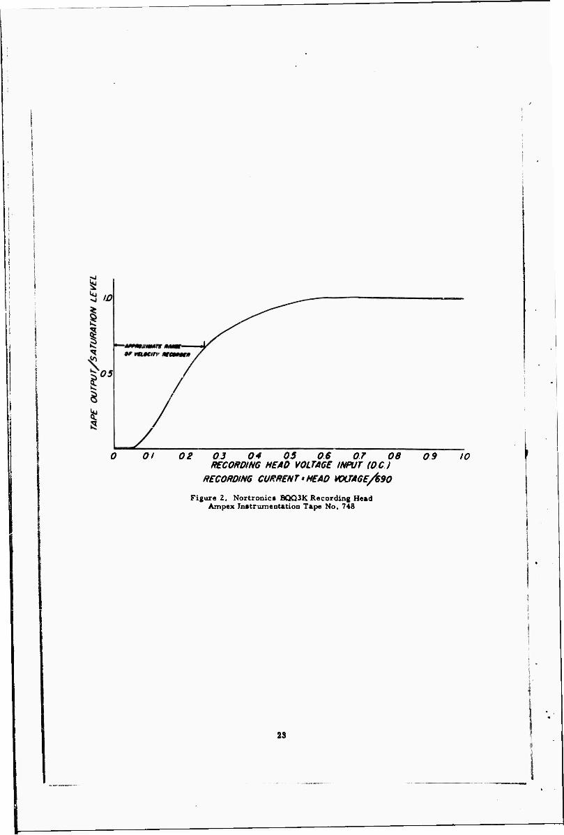
I

01 02 03 04 05 06 07 OB ReCOROING HEAD VOLTAGE INPUT (DC)

RECORDING CURRENT'HEAD WJAGE/GSO

Figure 2. Nortronics BQQ3K Recording Head Ampex In»trument»tion Tape No. 748

0 9 10

23

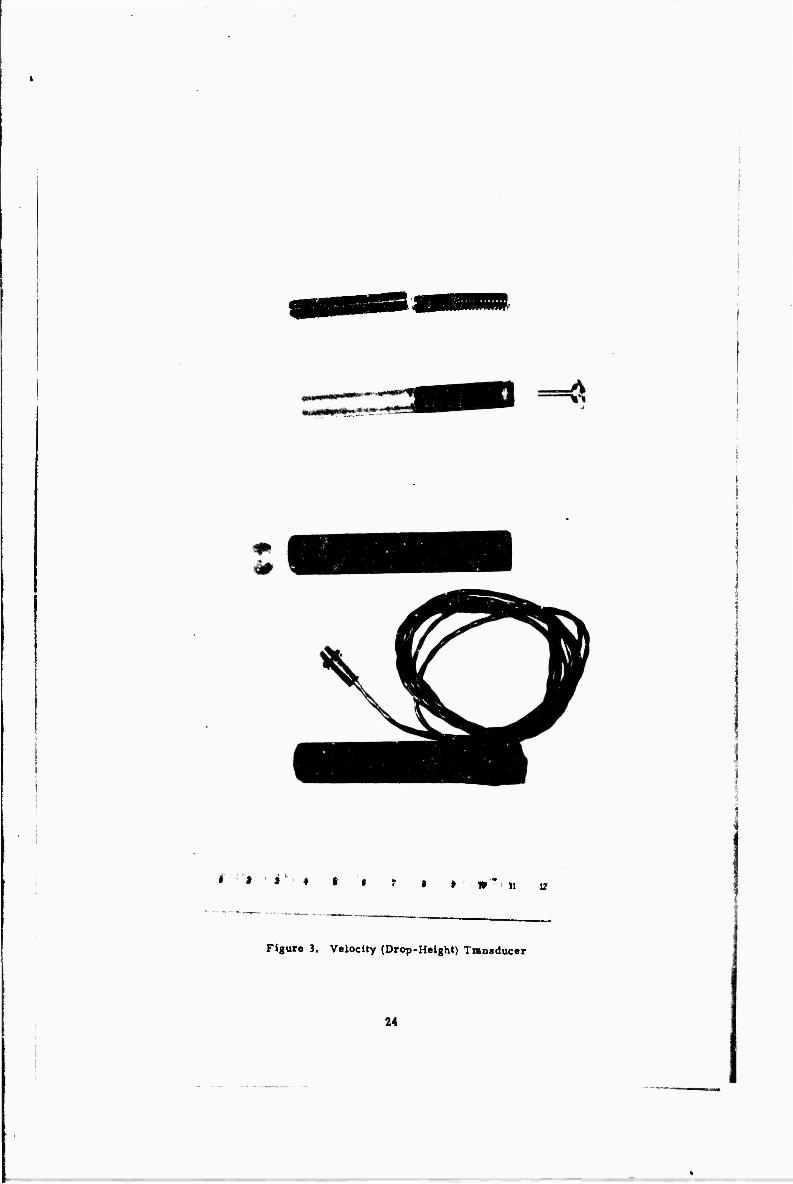
jr ; j - i ••. ♦ | • » i» ii i?

Figure 3. Velocity (Drop-Height) Tmnsducer

24

SHOCK INPUT TO TRANSDUCER — 12 INCH no tft« no«» iso« nm ton

TRANSDUCER RESPON$E — 12 INCH DROP HEIGHT iA raaiiva.TMi-iiva.it > «ft« VOITMC- 5 VOLTS

HEIGHT

Figure 4

it»

SIGNAL r>WM

TRANSDUCER

SIGNAL TO

MAGNETIC HEAD

5

la

5

" T '•MY;

SIGNAL FROM

MAGNETIC TAPE

Figure 5, Wavenhapei of Typical Velocity Signal During Acquitition, Recording and Playback

25

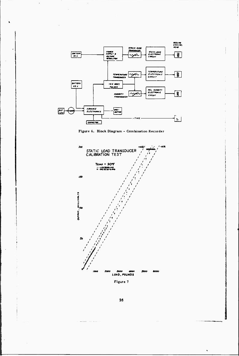
tMTtfr twnr » MtrMf

UTItDr *$ ¥

&© "

JTIMMP «ur mtmsivct*

*sy&* tTMTiC LO*» Ulcrmmc emtuii

rmtmovct» '—

«JO mue

ILtCtllOKIC emcuir

s^^&s

ttmitci MtTKOmCS

HJ ,cr

I tAfMrn»

Mi m/awrr

emevir 1

^J

Figure 6. Block Diagram - Combination Recorder

tOO ♦«»'■ / .; '-to*

STATIC LOAD TRANSDUCER / "9/ CALIBRATION TEST / /' '

/ " / / / /

TfMH • JOT / '. / • - «tCmNDlN« / ' • / • -»■«car-aMS / ,

/ '• / 1»

/ ' / / '. / / ' /

/ ', / r / /• / 1 / /•/ ^ / '» /

/ ' / */« ' '/ /

i / ' ■ /

, ' ■ 1

1 '. 1 ' ■ /

/ '• / 1 '.' '

So , i •

•' / 1000 JOOO 40OO 3000

LOAD,POUNDS

Figure 7

26

internal RC time constant and whose amplitude depends upon the operating potential. The output of the uni-vibrator is fed to the temperature lentor which consists of a voltage regulator and a bridge circuit and tc the humidity transducer consisting of a voltage regulator and an amplifier. The bridge circuit of the temperature sensor contains two temperature dependent thermistors and two equivalent calibration resistors. The output of the amplifier in the humidity sensor, is dependent upon the input bias which is a function of the electro- humidity transducer. The static load power supply modules, activated by the pulse from the uni-vibrator, supplies pulse excitation to the static load cell bridge whose output is proportional ' * the load being measured. This output is then amplified, converted to a D. C. level and fed to the recording head. Using these transducers the combination recorder is capable of measuring temperature from -50oF. to +150°F., humidity from 10% R. H. to 90% R. H. and static loads from 0 to 6000 pounds. A calibration curve for the static load system is presented in Figure 7.

3. Dynamic Load Recorder.

The dynamic load recorder consists of the basic recording unit married to three sets of dynamic load transducers mounted in three mutually perpendicular planes. The operation of this recorder is simiXcr to the static load portion of the combination recorder except that it is force actuated. The transducers, each consisting of four load cells connected in series, can be used to measure both static and dynamic loads.

DATA RETRIEVAL SYSTEM

The tapes containing data are processed using a data retrieval system (Figure 8). The data recorded is in the form of pulses whose amplitude and polarity ar« proportional to the parameter being measured. The system accepts data from the four parallel data channels, three containing analog data and the fourth containing timing information. Each analog data point consists of either a positive leading pulse or negative leading pulse in which the peak amplitude is proportional to some physical quantity. The amplitude and polarity of the leading data pulse is recognised, measured and recorded by the system. A fourth analog data channel is generated in the system by combining the velocity vectors from the three velocity channels and computing the equivalent impact height. At least one of the four input channels from the tape must contain information before the system will generate a read command.

The system consists of a control panel, a tape playback unit, a programmer, an analog to digital converter, a high-speed electro-optical printer, a two-pen recorder, and power supply racks. With the exception of the programmer and the control panel, all the equipment is commercUlly available. The programmer serves to interface and control the various equipment and consists of commercially available plug-in digital models. Some special circuitry used in this unit for signal conditioning and control are built on plug-in boards similar to the purchased logic plug-in boards.

Using this system, the tape is played back at 1-7/8 ips and the pulses fed to the peak memory drivers (Figure 9). The initial print signal is then fed to the high-speed optical printer initiating a line of print. Simultaneously, the peak signal amplitude is stored by the peak memory, scaled to engineering units by the output amplifiers, and fed to the analog to digital converter in proper sequence as determined by feed- back from the electro-optical printer. When the retrieval system is used for the velocity mods, the signal output from the peak n.emory is alno f'tl through a set of squares to summing amplifiers and then to the multiplex sequencer. Specifications for the system are as follows:

1. Three Modes of Operation:

a. Velocity.

b. Combination (Temperature, Humidity and SUtic Load).

c. Dynamic Load.

2. Logging rate-30 lines/sec.

3. Input rate up to 150 data pulses/ sec.

4. Time to retrieve and process six months of data (57, 000 data pulsas maximum) less than 10 minutes.

scale. 5. System Accuracy - *1%, full

Stability- Drift from Calibration 0. 05%/day 0. 01%/QC.

STATUS

Development work on the shock (drop- height) recorder and combination recorder has been completed. The shock recorder is estimated to cost less than $2500 each. The dynamic load recorder is 90% complete.

27

1

Figure 8. Data Retrieval Syitem

2°

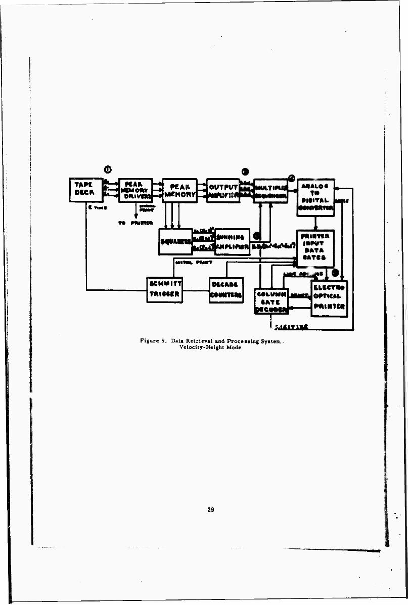
0 0

TA« DCCK

KAA

l «•••■ T FCAK

DRivtM -• MtMonr -, Mfttf::

T» piuvn«

OUTPUT

ItMIIII»« MfNflH

HNWb MMTT

KMMIfT VAlMfll

MCA»t leOLUMNlMMSi

tssssar— hiilillMJL

emcM.

Figure 9. Data Retrieval and Proceating Sytten Velocity-Height Mode

29

Work on an acceleration recorder Is continuing at the Natick Laboratories. The recorder will measure and record the deceleration forces, ir gravitational units, that packaged items received during transportation and storage.

LIMITED TESTS

A limited field test shipment from Natick Laboratories to Fort Lee, Virginia, with an intermediate stop at Tobyhann» Ordnance Depot «as made using the 12 shock (drop-height) recorders. The test shipment consisted In part of 512 No. 10 can slM Containers each of imitation maple syrup,(gross weight 60 pounds), dried dehydrated potatoes, (gross weight 21 pounb), and pea«, (gross weight 47 pounds). In addition 20 unitired loads. 40 x 48 x 54-1/2 Inches, (gross weight 1840 pounds), were also Included In the shipment. Nine individual shipping cases were instrumented with the shock recorders, three each weighted to simulate the cases of Imitation maple syrup, dried dehydrated potatoes and pea«. Three of the unit loads were also instrumenied with recorders.

In concept, participants would include recorders in shipments made by them, and furnish the resulting magnetic tapes together with other pertinent Information regarding the shipments to the Natick Laboratories. The tapes would then be processed and a copy of the print-out in digital form furnished to the shipper. Recorders would be acquired by the participants at their own expense using manufacturing data furnished by the Government or by loan of Government-owned recorders to the extent available. In this manner, a considerable amount of data would be acquired in a relatively short period.

REFERENCE

(1) M.A. Venetoi, "Development of Velocity Shock Recorder for Measurement of Shipping Environ- ments", The Shock and Vibration Bulletin 36, Part 6, pp. 173, Feb. 1967.

Analysis of the data received Indicated that the intensity and frequency of occurrence of handling shocks may b« far less than is cotnmoaly assumed. Test data also indicated that palletisation of supply items is effective In reducing the shock hazards which containers experience In shipment. The average di op-height was found to be 14 inches with a maximum of 28 inches. The containers were subjected to 18 handlings apiece and were subjected to two to three impacts each. Some minor deficiencies wfcre noted during the test. Most notable was a high quiescent current drain which decreased battery life considerably. This drain was traced to the activating switch which has been redesigned ;o reduce this drain tenfold.

FUTURE PLANS

At present, the most effective method of using the various» recorders has not been determined. Test shipments are not only costly and time consuming, but probably do not give a true indication as to what is actually happening In the field. The largest amount of significant information could be obtained in the shortest period of time by placing the recorders In actual shipments. It is planned to establish a Data Gathering Program, with participation by other Government Agencies as well as Industry.

This paper reports research undertaken at the U. S. Army Natick (Mass) Laboratories and has been assigned No. TP 543 in the series of papers approved tor publication. The findings in this report are not to be construed as an official Department of the Army position.

30

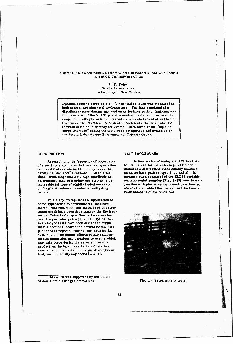
NORMAL AND ABNORMAL DYNAMIC ENVIRONMENTS ENCOUNTERED IN TRUCK TRANSPORTATION

J. T. Foley Sandla Laboratories

Albuquerque, New Mexico

Dynamic Input to cargo on a 2-1/2-ton flatbed truck was measured in both normal and abnormal environments. The load consisted of a distributed-mass dummy mounted on an isolated pallet. Instrumenta- tion consisted of the ELI 31 portable environmental sampler used in conjunction with piezoelectric transducers located ahead of and behind the truck/load interface. Vibran and Spectra are the data reduction formats selected to portray the events. Data taken at the "input-to- cargo interface" during the tests were categorized and evaluated by the Sandia Laboratories Environmental Criteria Group.

INTRODUCTION

Research into the frequency of occurrence of situations encountered in truck transportation Indicated that certain incidents may occur that border on "accident" situations. These situations, producing transient, high-amplitude accelerations, may be a prime contributor to ca- tastrophic failures of rigidly tied-down car >o or fragile structures mounted on mitigating pallets.

This study exemplifies the application of some approaches to environmental measurements, data reduction, and methods of interpretation which have been developed by the Environ- mental Criteria Group at Sandia Laboratories over the past nine years [1, 2, 3). Special research-type tests have been devised to supple- ment a continual search for environmental data published in reports, papers, and articles [2, 4, 5, 6, 7). The testing efforts relate environmental intensities and durations to events which may take place during the expected use of a product and include presentation of data in a manner which is useful to design, development, test, and reliability engineers [l, 2, 8].

TEST PROCEDURES

In this series of tests, a 2-1/2-ton flatbed truck was loaded with cargo which consisted of a distributed-mass dummy mounted on an isolated pallet (Figs. 1. 2, and 3). In- strumentation consisted of the ELI 31 portable environmental sampler (Fig. 4) [9] used In conjunction with piezoelectric transducers located ahead of and behind the truck/load interface on main numbers of the truck bed.

This work was supported by the United States Atomic Energy Commission. Fig. 1 - Truck used in tests

31

Fig. 2 - Load in truck tests Fig. 3 - Load in truck tests

Fig. 4 - ELI 31 portable environmental sampler

32

The general procedure was to drive over the route chosen, isolate certain conditions which might produce unique dynamic environments, and sample the events. The route started in Amarillo. Texas, and continued west to the Texas/New Mexico border on U.S. 66 and Interstate 40. Events sampled along this route wh3ch were considered normal environments were:

1, Backing up tc loading dock across RR tracks (Fig. 5). (Vibran)

2. Driving to weighing station over a series of RR tracks. (Vibran and Spectra)

J. Going into a dip at 15 mph. (Vibran)

4. Driving from a low, level road to a raised road. (Vibran)

5. Driving onto bad overpass at 50-55 mph. (Vibran)

6. Driving on heavily patched asphalt highway at 50 mph. (Vibran)

7. Driving on access road parallel to inter-" state highway. (Vibran)

8. Driving on smooth blacktop, four-lane interstate highway at 50, 55, and 35 mph. (Vibran)

9. Driving in paved construction zone at 45 and 55 mph. (Vibran)

10. Driving on rough blacktop at 60 mph, (Vibran)

TABLE 1

Truck Test Inatrumentation Direc^orv Calibrate Values on Data Tape

EU 31 Channel

No. Location in Tc.

1 V - Truck bed, aft of pallet on ^ 2 L - Truck bed, aft of pallet on ^ 3 V - Truck bed, fwd of pallet on f, 4 L - Truck bed, fwd of pallet on f, 5 T - Truck bed. fwd of pallet on ^ 6 L - L«.f* »-«ar, load mount 7 V - Left rear, load mount 8 T - Right front, load mount 9 V - Right front, load mount

10 L - Top of dummy load 11 T - Top of dummy load 12 V - Top of dummy load 13 480-cpa servo time base 14 Voice channel

V = vertical axis L * longitudinal axis T * transverse axis

Instruments: ELI 31 recorder Dictaphone Citizen's band trans-

ceivers

Fig. 5 - Loading dock and railroad track employed in tests

Samples taken in a second series were of abnormal situations which might occur along the route and which could produce severe environmental {npiits. These were as follows:

1. Colliding with loading dock. (Spectra)

2. Driving over RR tracks at high speed, 45 and 50 mph. (Spectra)

3. Driving with two wheels on the shoulder at 45 mph. (Vibran)

4. Driving completely on the shoulder at 45 mph. (Vibran)

5. Driving off the road in desert brush (Fig. 6). (Vibran)

6. Driving Into a dip at 50 mph. (Vibran)

7. Driving onto the median of an interstate highway (turning around). (Vibran)

8. Hitting poi holes In a truck stop at 45 to 50 mph. (Spectra)

9. Driving on a dirt road at 45 mph. (Vi- bran)

10, Running over a cattle guard at 45 mph (Fig. 7). (Spectra)

33

Fig. 6 - Dirt road and desert brush in area where tests were conducted

Fig. 7 - Typical cattle guard over which environments were sampled

DATA REDUCTION

The descriptive terme, Vibran (vibration analysis) and Spectra (response spectra of single-degree-of-freedom systems), indicate the data reduction format selected to portray the event [2, 3, 4]. Figure 8 is an example of the Vibran data format. Spectra data format is illustrated in Figs. 10. 12, 14, 16, and 13.

DATA EVALUATION - NORMAL ENVIRON- MENTS

Long-Duration Phenomena -- Program Vidar (Vibran data reduction [2])was utilized to analyze the normal environments of long duration. The following functions were performed:

1. The vertical axis was selected as being the axis in which maximum acceleration levels were detected.

2. The Vibran data from the two truck-bed vertical pickup locations were combined into a composite acceleration density description of the dynamic environment for each of the normal events sampler*

3. A tabulation of frequency of occurrence of road types [2] was used as a guide to obtain weighting factors for each of 'he ten events. These weighting factors were then applied in the production of a composite acceleration probability density description of the environment produced in the vertical axis at the truck/load interface. Table 2 gives the resulta»t acceleration probability description of a trip in which these ten road types would be encountered. Table 3 lists the weighting fac irs that were applied to each road type when generating the composite environment description.

Transient Phenomena -- One normal event, considered to be sufficiently transient to warrant analysis in terms of shock spectra, was the crossing of railroad tracks at slow speed. Figure 9 presents the vertical g-time history of this event; Figure 10 presents the resultant shock spectra, with the responding single-degree-of-freedonr. systems assumed to have critical damping ratios of 0, 0.03, and 0.10.

In general, spectra depict the response transient truck transport environments taken at the payload/truck-bed interface are interpreted by the Environmental Criteria Group as follows:

1. Shock spectra picture the response severity on cargo.

2. The 0. 03 damping spectrum is an estimate of the response severity produced on nonisolated cargo systems.

3. The 0.10 damping spectrum is an estimate of the response severity produced on isolated or mitigated cargo systems.

34

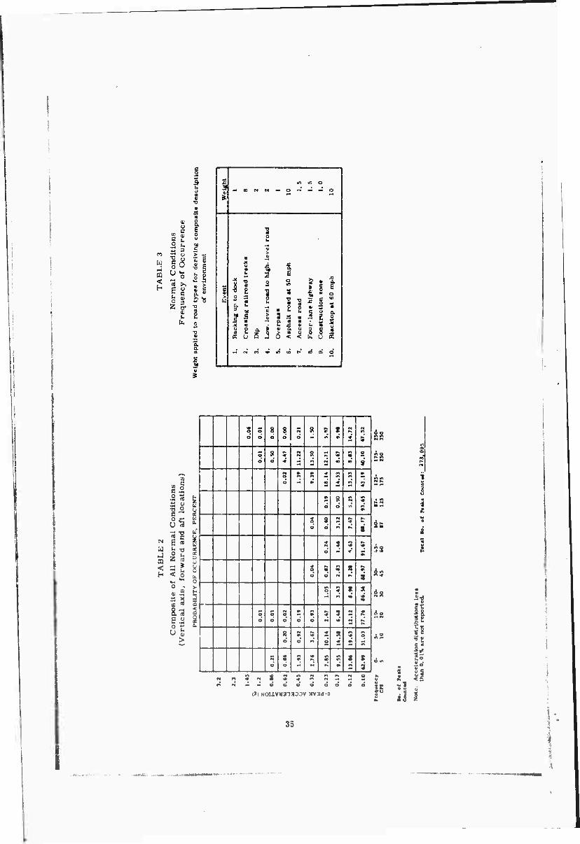
u s u r i

10 0 c u

4-1

u 3 ?

m

Cd 0 a g c

1 0 ■o

ffl U 0 u

< on >! h E 0

B i

2 3

01

£ 0

if

-a - -« — o

£

2 f

s *<

O O

O o

8 o

8 o o

s ^

1—i

S *

M

<•

o o

a o

5 >#

1«« 5? N

O

9

3 • •> <* ri

4

o S

o s 5

s

^ 1 cd g

•2 S

o *•* 3 1^ <•

7

3 o

tu a s

1 t o 5 •

St i

o o

o o

o o

m o

s o

5 •

ft s

u 01 > 8

o s o

<• s

R ■*

9 *

o

M e

s o

s <• N 1

8 ■A

* « « 3

^S

is

5S

do ft «St

AS

4 N /t n rt

-' o o o o o

(») NOIiVH3aa33V 5(V3d-0

35

St If Si i

Is id

il i !•.

»CCILIimnON DISTRISUTKM, «IICEST

• 1.2

g 0.65

»■ 0.23 o

0.17

0.12

O.iO

S.M

0.00

!.♦* Driving off r aad in deseri brush.

0.00

0.00

0.00

0.00 1.3«

J.»3 9.U 0.S2

u.t« .o.U 10. }3 0.42 O.iO 0.70 '

35.2« 2«. 3« 1.7« 0.71 O.H «.«« ■•1 5.91 0.00 |

U.M tt.20 n.ts 3.01 l.*2 0.13 0.10 15.*5 0,85 {

20.tt 32.4« •«.3« »«.27 97.M 84.05 w.ts •7.71 77.25 99.15 |

Frequency 0- crs 5

5- 10

10- 20

20- 30

30- 45

45- 60

60- 87

87- U5

125- 175

175- 250

250- 350

to. et Fiiki Counted

54 74 227 «01 U2 »37 769 1701 2321 3270 4770

Totti Ho. of Hakl Counttd: 15,021;

Fig. 8 - Example of Vibran format

4. The 0. 0 spectrum is an estimate of the up^sr limit of response severity which •i, y be achieved in the first application of a series of pulses of the type from which spectra were obtained regardless of the damping which may be present in the system.

b. In specific evaluations, cargo responses greater than those predicted for 0.0 damping indicate that it is questionable whether the system under consideration approached a single-degree-of-freedom system.

The shock spectra shown in Figure 10 are those derived for the pickup location at the rear location on the truck bed. These spectra envelop the spectra obtained at the forward location on the truck bed and are, therefore, considered to represent the greatest vertical axis response severity relative to location of cargo on the truck bed.

DATA EVALUATION - ABNORMAL ENVIROM- MENTS

Long-Duration Phenomena -- The following events were considered to occur over a period of time which precluded their interpretation as trEnsient phenomena:

1. Driving with two wheels on the shoulder at 45 mph,

2. Driving completely on the shoulder at 45 mph.

3. Driving off the road in desert brush.

4. Driving into a dip at 50 mph.

5. Turning around on the median of a four- lane highway.

6. Driving on a dirt road ai 45 mph.

■H

:

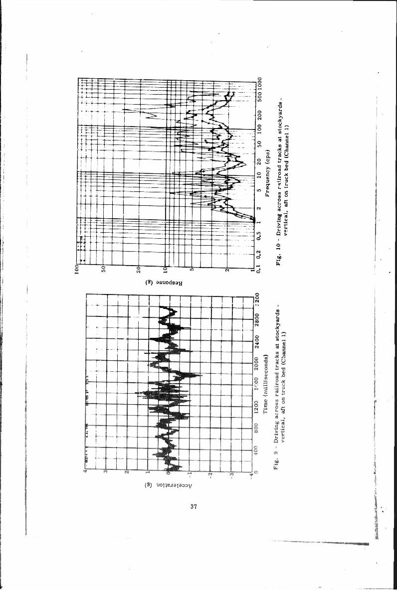
m _ <-. 4) to c

Ü ■D V

XI

o 3

U

V a o C

(8) ssuodsaH

(8) U0TJBJ3X3DDV

37

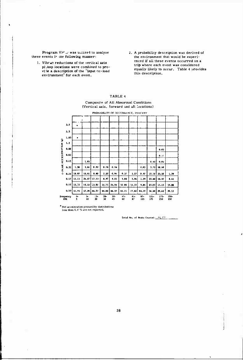
Prograin Vi'' _• was uiiüzed to analyze these events i"- cne following manner:

i, Vlbr^C reductions of the vertical axis pi.kup locations were combined to pro- vile a description of the "input-tc-load environment" for each event.

A probability description was derived of the environment that would be experienced if all these events occurred on a trip where each event was considered equally likely to occur. Table 4 urovides this description.

1.2

l.i

t 0.1

u O 0.43 <

u 0. a 0.23

O.U

a.io

TABLE 4

Composite of Ali Abnormal Conditions (Vertical axis, forward and aft locations)

PROBABILITY OF OCCt'RhfcNCE, PFRCENT

I

•

«

0.05

0.5A

1.13 0.41 0.04

1.» 3.»1 0.« 0.74 0.14 0.05 3.71 IS.43

It.17 H.4I t.tc 2.32 O.t« 0.37 2.27 0.»7 15.U 23.10 1.5«

13.13 24.37 17.13 «.»7 t.02 5.04 5.»» 2.3» 23.40 14.»7 (.41

15.!5 14.33 i3.«2 21.75 24.54 12.«4 14.22 •,M 23.03 13.15 1«.M

51.55 32.2« 44.57 «4.00 44.37 SI.71 77.42 tt.n i

34.20 20.43 70.12

Irtqvmacy S- 5- ;o- 20- 30- 4^- te- 17- 123- 175- 250- CT» J !0 20 30 ts 60 ll 125 175 250 350

* Net acceleration probability distributions lean than 0o Ö"\ ar« not reported.

Total Ko. of Peak» Counted: 93. 1'

38

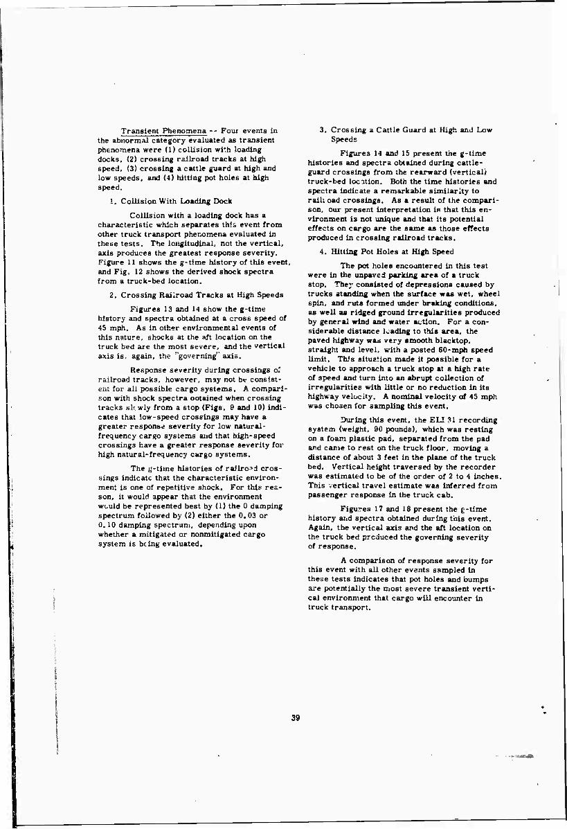
Transient Phenomena -- Four events in the abnormaj category evaluated as transient phenomena were (1) collision with loading docks, (2) crossing railroad tracks at high speed, (3) crossing a cattle guard at high and low speeds, and (4) hitting pot holes at high speed.

1. Collision With Loading Dock

Collision with a loading dock has a characteristic which separates this event from other truck transport phenomena evaluated in these tests. The longitudinal, not the vertical, axis produces the greatest response severity. Figure 11 shows the g-time history of this event, and Fig, 12 shows the derived shock spectra from a truck-bed location.

2. Crossing Railroad Tracks at High Speeds

Figures 13 and 14 show the g-time history and spectra obtained at a cross speed of 45 mph. As in other environmental events of this nature, shocks at the aft location on the truck bed are the most severe, and the vertical axis is, again, the "governing" axis.

Response severity during crossings or railroad tracks, however, may not be consistent for all possible cargo systems. A comparison with shock spectra obtained when crossing tracks sk wly from a stop (Figs. 9 and 10) indicates that low-speed crossings may have a greater response severity for low natural- frequency cargo systems atid that high-speed crossings have a greater response severity for high natural-frequency cargo systems.

The g-time histories of railroad crossings indicate that the characteristic environment is one of repetitive shock. For this reason, it would appear that the environment would be represented best by (1) the 0 damping spectrum followed by (2) either the 0.03 or 0.10 damping spectrum, depending upon whether a mitigated or nonmitigated cargo system is being evaluated.

3. Crossing a Cattle Guard at High and Low Speeds

Figures 14 and 15 present the g-time histories and spectra obtained during cattle- guard crossings from the rearward (vertical) truck-bed iocition. Both the time histories and spectra indicate a remarkable similarity to rail, oad crossings. As a result of the comparison, our present interpretation 1« that this environment is not unique and that its potential effects on cargo are the same as those effects produced in crossing railroad tracks.

4. Hitting Pot Holes at High Speed

The pot holes encountered in this test were in the unpaved parking area of a truck stop. They consisted of depressions caused by trucks standing when the surface was wet, wheel spin, and ruts formed under braking conditions, as well as ridged ground irregularities produced by general wind and water action. For a considerable distance loading to this area, the paved highway was very smooth blacktop, straight and level, with a posted 60-mph speed limit. This situation made it possible for a vehicle to approach a truck stop at a high rate of speed and turn into an abrupt collection of irregularities with little or no reduction in its highway velocity. A nominal velocity of 45 mph was chosen for sampling this event.

During this event, the EL! 31 recording system (weight, 90 pounds), which was resting on a foam plastic pad, separated from the pad and came to rest on the truck floor, moving a distance of about 3 feet in the plane of the truck bed. Vertical height traversed by the recorder was estimated to be of the order of 2 to 4 inches. This vertical travel estimate was inferred from passenger response in the truck cab.

Figures 17 and 18 present the g-time history and spectra obtained during this event. Again, the vertical axis ar>d the aft location on the truck bed produced the governing severity of response.

A comparison of response severity for this event with all other events sampled in these tests indicates that pot holes and bumps are potentially the most severe transient vertical environment that cargo will encounter In truck transport.

39

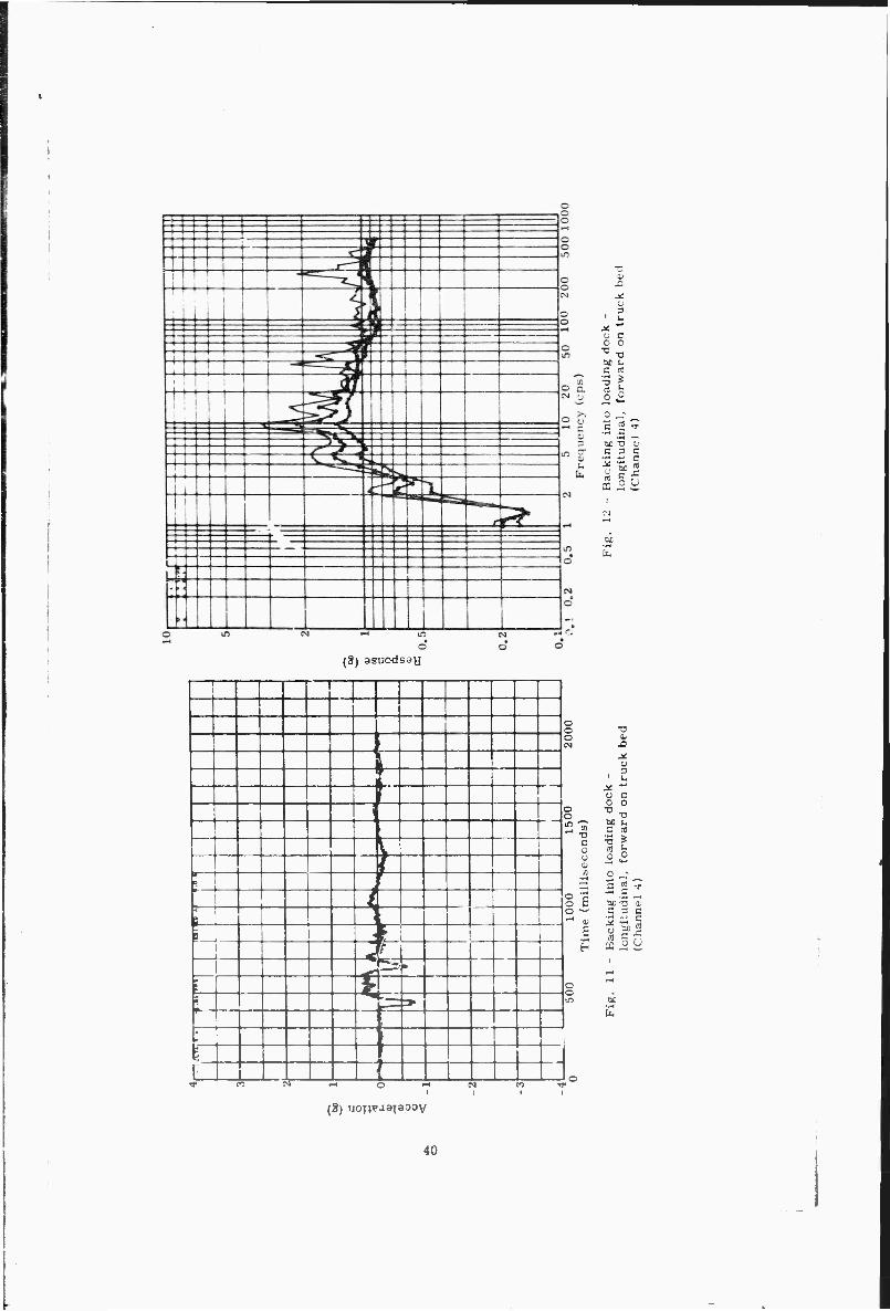
<J c o o

10 13

C ™ l1

C 3 c

(3) asuodsay

J L

o o

c o u o

0 c O E O -'

0 3

1 Li

Ü C 0 o

c 2 ' e* -a oi •S H S

(3) uoppaaiaoov

40

&&=& -r- =*=4 o ^ 1 '

1 0

.2

0.

5

1

2

5

10

2

0

5

0 1

00

200

5

00

Fre

qu

ency

(cp

s)

s -/ - r T -J ■^- "^^ _- ^,

i

U—^T 5.

-^=1 a ^__ J— q -—:T v

^H^ i \= ^S^ L ** >

r ! I 1 . i I 'v ' ——. p^

T ■ 1 [ ct_ •*^- ä^V

IS 1

F^

i i i i i *=?

S^i ^ 4- i— t—

i—1— bM 2 8 ^ ^ 8^ i

t pp- \*i ' i i <^L ; ; j. t—

i

—}—

"=*fc -=^=

-rrr-i- —t— — til! •

♦ ÜTT 1 i 1 1 1! :►: : ' i ! 1 J M

H i i b

o o

c o o in Lt •*

(2) asuodsa^}

o

i

o o o CM

o o in tH ^^

01 •o c 0 u 01 ID

§1 o j:

6 H

o o m

| i

i Ä I JK *■

e_ ^ m -<

1 I j

i * i to § t

1 a -■i b So

j _^ ! I

0 j« 1 1

I ^

t~ 1 •a 2 * 1 j

m 1 i s 1 ■ s§

> 1 ^mm „g "" 2i i - —* +*! -

"" S o

« «■ T1 »■ ; H ■■ ■ Q >

t—t- - 1

o

W 1

Km

to <-H

; T •- S1

1 t

-4 4 ^ P >> e

(3) uoi ao

41

N ■

5.°

_ o Q 5=- f4- »-J

^^ "l 2 •—^ < wjS. \

-^_ t ^ J^JW ^ -

'*£■ _

AC i

■ ■MM.

■«=;

^^i! j^^

'1 T = -; = :ss ■TT-»- -^— 0 -a 3 * | ■ ■ u t -?^ 10 ^5 1 •<" ^^

1

l ! i «* % ■^ 1

s-- 1 1 .. s ^

T¥ :1^= . w- 11 ' i 11 ^<:J y f Si i \ ^ ^L. 1 ^ ** --

■U 4=^ r

1

2

Dri

vin

g ver

tica

ri 1— ;. O <D

.5; t T N M

f o U.

° o o m N - •« CM -<

(8) asuodBaa

o

1 f i . • ^«S r . 6^

1 5 K, ! i

—*J

m o -oO

1

"""

15

ds}

e gu

a k

bed

J . § HS

n jäjß pi" 5} Si jm^T §3 S§

| ^3j B' 2| 2i i »3 fr « «-^ aia H. •5 -S^

_^ S M Sdr h t* i i 3Ba K =. o Ö > • ^g 5 ^^-ri*--- L "5 ' m

m i _.-, ^^

irr ■ I CSi EL 6t

1H

I a Kp. . fa

T! EL. * r e ̂

(8)

-« o

uop«aats DOV

l-t

t ■ "f * ■<

o

42

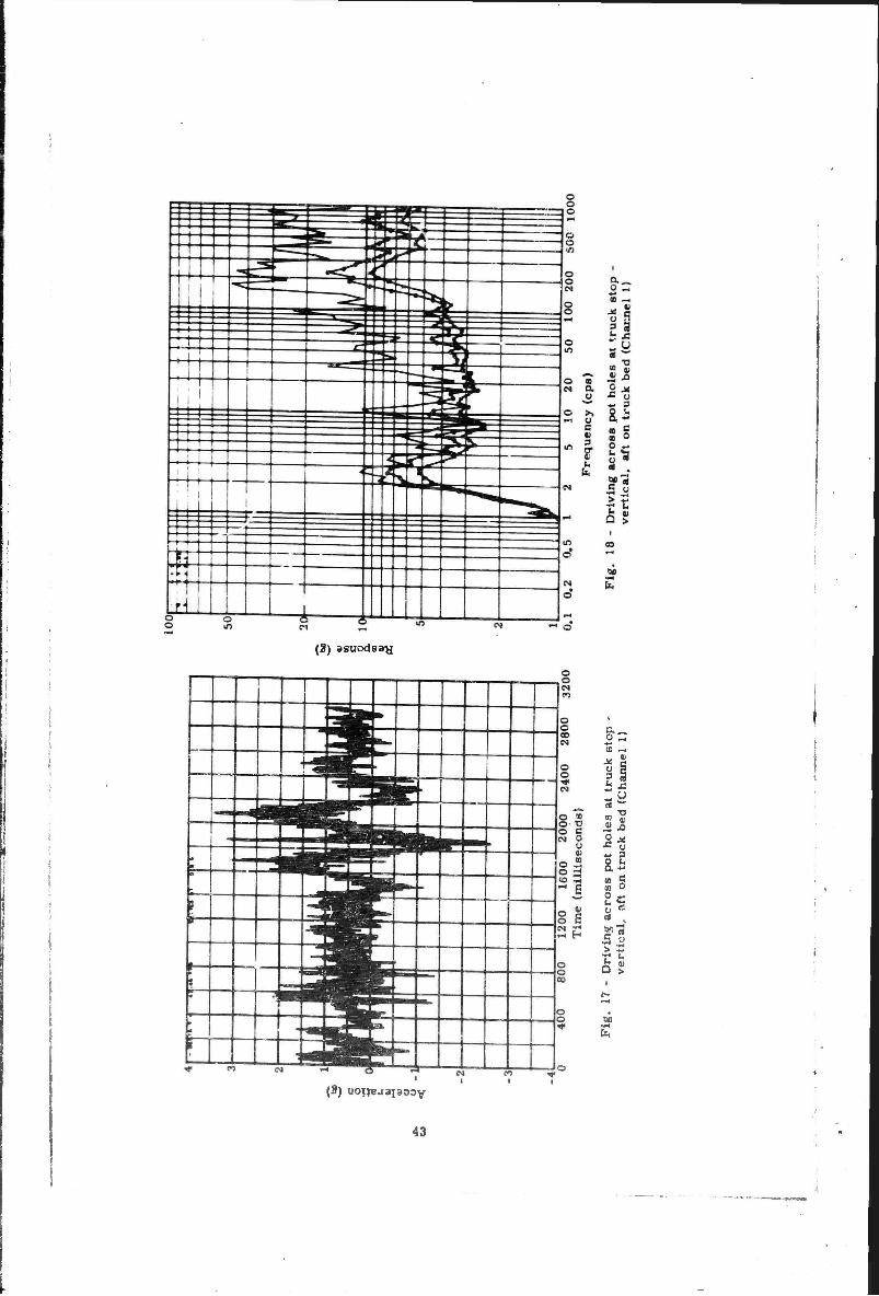
(8) ssuodsaH

o «

* a

ii ■=

»'S Ü -5

II

an

(8) uoTjcaapoov

43

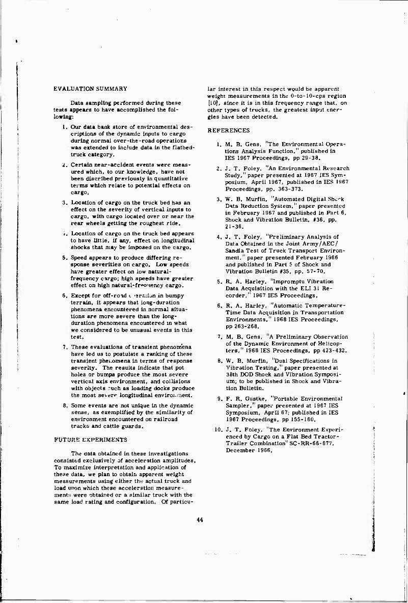
EVALUATION SUMMARY

Data sampling performed during these tests appears to have accomplished the following:

1. Our data bank store of environmental descriptions of the dynamic inputs to cargo during normal over-the-road operations was extended to inc.'ude data in the flatbed- truck category.

'i. Certain near-accident events were measured which, to our knowledge, have not been discribed previously in quantitative terms which relate to potential effects on cargo.

3. Location of cargo on the truck bed has an effect on the severity of vertical inputs to cargo, with cargo located over or near the rear wheels getting the roughest ride.

i. Location of cargo on the truck bed appears to have little, if any, effect on longitudinal shocks that may be imposed on the cargo.

5. Speed appears to produce differing response severities on cargo. Low speeds have greater effect on low natural- frequency cargo; high speeds have greater effect on high natural-fr*»anency cargo.

6. Except for off-road i ^rr.ci^n in bumpy terrain, it appears that long-duration phenomena encountered in normal situations are more severe than the long- duration phenomena encountered in what we considered to be unusual events in this test.

7. These evaluations of transient phenomena have led us to postulate a ranking of these transient phenomena in terms of response severity. The results indicate that pot holes or bumps produce the most severe vertical axis environment, and collisions with objects such as loading docks produce the most severe longitudinal enviroi,:aent.

8. Some events are not unique in the dynamic sense, as exemplified by the similarity of environment encountered on railroad tracks and cattle guards.

FUTURE EXPERIMENTS

The aata obtained in these investigations consisted exclusively of acceleration amplitudes. To maximize interpretation and application of theae data, we plan to obtain apparent weight measurements using either the actual truck and load ur'on which these acceleration measurement» were obtained or a similar truck with the same load rating and configuration. Of particu-

lar interest in this respect would be apparent weight measurements in the O-to-10-cps region [10), since it is in this frequency range that, on other types of trucks, the greatest input ener- gies have been detected.

REFERENCES

1. M. B. Gens, "The Environmental Opera- tions Analysis Function," published in IES 1967 Proceedings, pp 29-38.

2. J. T. Foley, "An Environmental Research Study," paper presented at 1967 IES Sym- posium, April 1967, published in IES 1967 Proceedings, pp. 363-373.

3. W, B. Murfin, "Automated Digital Shck Data Reduction System," paper presented in February 1967 and published in Part 6. Shock and Vibration Bulletin, #36, pp. 21-36,

4. J. T. Foley, "Preliminary Analysis of Data Obtained in the Joint Army/AEC/ Sandia Test of Truck Transport Environ- ment," paper presented February 1966 and published in Part 5 of Shock and Vibration Bulletin #35, pp. 57-70.

5. R. A. Harley, "Impromptu Vibration Data Acquisition with the ELI 31 Re- corder," 1967 IES Proceedings.

6. R, A. Harley, "Automatic Temperature- Time Data Acquisition in Transportation Environments," 1968 IES Proceedings, pp 263-268.

7. M. B. Gens, "A Preliminary Observation of the Dynamic Environment of Helicop- ters," 1968 IES Proceedings, pp 423-432.

8. W. B. Murfin, "Dual Specifications in Vibration Testing," paper presented at 38th DOD Shock and Vibration Symposi- um; to be published in Shock and Vibra- tion Bulletin.

9. F. R. Gustke, "Portable Environmental Sampler," paper presented at 1967 IES Symposium, April 67; published in IES 1967 Proceedings, pp 155-160.

10. J. T. Foley, "The Environment Experi- enced by Cargo on a Flat Bed Tractor- Trailer Combination" SC-RR-66-677, December 1966,

44

DISCUSSION

Mr. Renlus (Army Tank Automotive Com- mand): Can you tell me what truck you used and why you used that truck? If you used more than one, was there any variation noted between trucks?

Mr. Foley: First of all, the truck that we used for this test was used because it was available. In this particular situation it was a piggy-back test for us. The truck and every- thing else was furnished by another organization. Actually, it turned out that we had two hours notice to take measurements on this truck, so we took the opportunity. We are also interested in trying to measure the variation from one truck to the next. The next time we get a crack at it we will do it. We just have not gotten around to it yet.

Mr Childs (SRDE): fully laden or light?

Were these trucks

Mr. Foley: The load was relatively light.

Mr. Childs: So the springs would be out of action ?

Mr. Foley: Yes. Another point, with regard to your paper, is that the load was all tied down, not loose.

Mr. Childs: So you are actually measuring the shock on the truck, not on the package.

Mr. Foley: lliat is right. We measured the input to the cargo and only thru the use of shock spectra inferring what this produces in the way of response.

Mr. Christo (Naval Underwater Weapons Research and Engineering Station): With re-

spect to laboratory tests, what would be the best test to simulate truck transportation?

Mr. Foley: TTiere is a reference concerning our views on this at the end of the paper. There is another reference on how to apply this sort of data to derivation of tests. Very roughly, I would say that you need three different types of tests. You need: a low level random vibration test, a repetitive shock test superimposed on a random background, and a very low frequency test - load applications which are very close to static equivalent loads. I think it has to be done in three steps to cover all the parameters.

Mr. Griffith (Bendix Missiles Systems Division): I am rather surprised at the levels of the normal events compared with the abnormal. Have you drawn any conclusions as to whether or not these may have been higher in the normal because of the light load?

Mr. Foley: Ulis is entirely possible. What we would like to io on things like this, though we did not have the opportunity here, is to run a range of loads.

Mr. Griffith: You pointed out that you are using primarily piezoelectric accelerometers. You had some frequencies that were extremely low. How did you obtain these?

Mr. Foley: The system utilized with the accelerometers is essentially a charge amplifier which we feel is good to 2 or 3 hertz. The plot Is wrong when it says 0 to 2-1/2 hertz. There is really no zero frequency there. I would have preferred to use plezoresistive types but the short notice for the test prevented this.

45

DEVELOPMENT OF A RAILROAD ROUGHNESS

INDEXING AND SIMULATION PROCEDURE

L. J. Pureifull and B. E. Prothro U.S. Army Transportation Engineering Agency

Military Traffic Management and Terminal Service Fort Eusti», Virginia

In order to simulate rail vehicle performance on an analog computer to study shock and vibration characteristics of various rail and cargo configurations, it is necessary to provide an input representing the roughness characteristic of the rail surface. This paper describes a study of methods for measuring and simulating rail surface roughness which resulted in a recommendation to use a white noise generator to provide the required inputs. Measured accelerations on cargo were found to approximate the characteristics of white noise. The measured acceleration values were correlated with descriptive adjectives good, fair, rough, etc., and were further correlated with causative displacement inputs to the railcar springs. Apian for measuring rail surface condition using an accelerometer at the base of the truck springs is described.

The U.S. Army Transportation Engineer- ing Agency (USATEA), Military Traffic Man- agement and Terminal Service, Fort Eustis, Virginia, is concerned with the effects of the transportation environment on military cargoes. One of the Agency's interests is to find better ways of predicting the characteristics and effects of shock and vibration that may be encountered in the land, air, or water modes of transport. The Agency uses an analog computer to simulate vehicle performance with various load configurations, but in order to do this, sufficient information about the vehicle must be known to write the equations of motion. In addition, it is necessary tobe able to specify the right-of-way variations that cause a vibratory response and to simulate these variations for input to the computer. Frequently, the most difficult part of the problem is to find a method for introducing the right-of-way characteristics.

This paper deals with only one mode, the rail mode, and describes the approach bein« taken to develop an index for classification of rail surface roughness, a method for simulation of the rail surface roughness for input to an analog computer, and a method for measurement of the rail surface roughness. Some of

the work is still in progress, and further proof- testing in the field is planned to verify the sound- ness of the Agency's methods. It is antic.'pated that the approach presented in this paper will stimulate further thought and research on the subject.

This study is limited to consideration of the vertical displacements of the surface profile of a railroad track. The track has other defined characteristics, such as warp, gage, superele- vation, cross level, and alignment, which may contribute to the shock and vibration environment, but the key factor to which the railcar suspension system responds is vertical surface roughness. It is also one of the most trouble- some factors in track maintenance.

At present, no common agreement exists as to how the surface roughness should be described. In conversations, such adjectives as smooth, rough, good, bad, etc. , are used, based on subjective impressions; but these terms have no meaning to a computer unless they are defined with qualitative values. That is the purpose of the railroad roughness index: to assign measurable qualitative limits to the descriptive adjectives customarily used so that the environment can be accurately expressed

47

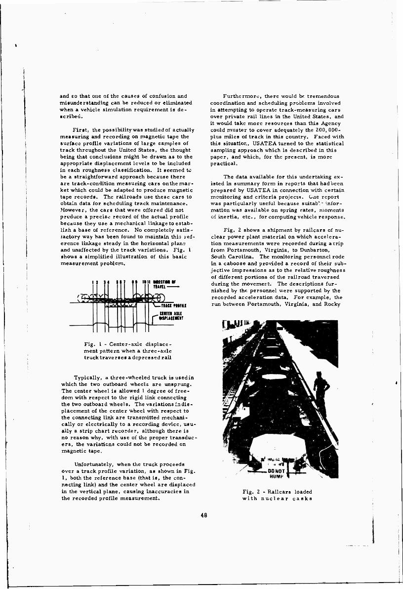
and so that one of the causes of confusion and misunderstanding can be reduced or eliminated when a vehicle simulation requirement is described.

First, the possibility was studied of actually measuring and recording on magnetic tape the surface profile variations of large camples of track thrcughout the United States, the thought being that conclusions might be drawn as to the appropriate displacement levels to be included in each roughness classification. It seemed to be a straightforward approach because there are track-condition measuring cars on the mar- ket which could be adapted to produce magnetic tape records. The railroads use these cars to obtain data for scheduling track maintenance. However, the cars that were offered did not produce a precise record of the actual profile because they use a mechanical linkage to establish a base of reference. No completely satisfactory way has been found to maintain thia »ef- erence linkage steady in the horizontal plans and unaffected by the track variations. Fig. 1 shows a simplified illustration of this basic measurement problem.

M UK MfCTMIM TUm

run ninic tinn HIE MflUIWIT

Fig. 1 - Center-axle displacement pattern when a three-axle truck traverses a depressed rail

Typically, a three-wheeled truck isusedin which the two outboard wheels are unsprung. The center wheel is allowed 1 degree of freedom with respect to the rigid link connecting the two outboard wheels. The variations in displacement of the center wheel with respect to the connecting link are transmitted mechani- cally or electrically to a recording device, usually a strip chart recorder, although there is no reason why, with use of the proper transducers, the variations could not be recorded on magnetic tape.

Unfortunately, when the truck proceeds over a track profile variation, as shown in Fig. 1, both the reference base (that is, the connecting link) and the center wheel are displaced in the vertical plane, causing inaccuracies in the recorded profile measurement.

Furthermore, there would bf: tremendous coordination and scheduling problems involved in attempting to operate track-measuring cars over private rail lines in the United States, and it would take more resources than this Agency could muster to cover adequately the 200,000- plus miles of track in this country. Faced with this situation, USATEA turned to the statistical sampling approach which is described in this paper, and which, for the present, is more practical.

The data available for this undertaking existed in summary form in reports that had been prepared by USATEA in connection with certain monitoring and criteria projects. One report v/as particularly useful because suitab" ■ information was available on spring rates, moments of inertia, etc. , for computing vehicle response.

Fig. 2 shows a shipment by railcars of nuclear power plant material on which acceleration measurements were recorded during atrip from Portsmouth, Virginia, to Dunbarton, South Carolina. The monitoring personnel rode in a caboose and provided a record of their subjective impressions as to the relative roughness of different portions of the railroad traversed during the movement. The descriptions furnished by the personnel were supported by the recorded acceleration data. For example, the run between Portsmouth, Virginia, and Rocky

Fig, 2 - Railcars loaded with nuclear casks

48

Mount, North Carolina, was described as "definitely rough". It had been so rough that sleep was practically impossible. Conversely, the run from Augusta, Georgia, to Dunbarton, South Carolina, was described aa "smooth". The report showed that the maximum acceleration recorded on the "rough" Portsmouth to Rocky Mount run was 0. 9g at 3 hertz, and the maximum acceleration on the "smooth" Augusta to Dunbarton run was 0,4g at 3 hertz. There- fore, a correlation of the abstract terms "good" and "rough" with corresponding measurable parameters is established. This correlation can be used as a starting point for development of a rail roughness index.

Next, it is necessary to determine whether the accelerations are truly random. If so, the possibility of simulating the roughness with a random noise generator is quite obvious. The evidence affirming this comes from two sources: one is the cumulative distribution of peak accelerations recorded during a rail trip at a constant speed, and the other is a plot of peak accelerations versus frequency contained in Army Tech:^cal Bulletin 55-100, Transport- ability Criteria - Shock and Vibration. I1)

Fig. 3 shows the cumulative distribution of peak accelerations recorded during a 65-mile- per-hour run between Rocky Mount, North Carolina, and Florence, South Carolina. This curve looked enough like a random distribution to encourage further investigation.

To determine better the degree of randomness, the cumulative distribution was divided into

0. Ig elements which were used to plot a probability density distribution. A normalized amplitude density curve having the same standard deviation as the data was superimposed for comparison. Fig. 4 shows this comparison.

It is apparent that there is a strong family resemblance. Ceitainly the plotted data do not ideally conform to a Gaussian distribution which would be characteristic of white noise. Even though distribution is skewed, it does not have the characteristic dips which would indicate cycling.

One possible explanation for the skewing is unequal sampling. For example, skewing would occur if two Gaussian distributions having unequal amplitudes were added. More research is needed in this area to develop a reliable sampling techniqv:.

To illustrate. Fig. 5 shows the route followed during the 65-mile-per-hour run. The trip totaled 173. 1 miles between Rocky Mount and Florence. Note, however, that there is a 74.2-mile section between Wilson and Fayettc- ville which would not normally be traversed by trains coming from the north or south to Wil- mington, a busy seaport. It seems reasonable to expect, therefore, that this section which did not receive as much wear and tear might be smoother than the 16. 1-mile section from Rocky Mount to Wilson and the 82. 8-mile section from Fayetteville to Florence. Such a difference: in the samples would account for skewing in the same direction as that noted in the probability density graph, and it points out the

2.0

1.5

Sl.l

= 0 5

- ; -M 'Jft i ■l.lh-

-M »—17 1.. — 21 — . }| l r i.i-

^

i ^_ " 1 l^i

-- P 10 21 31 «I SI •• 71

CUKUUIIH IISTIIIITIH |%| II IIS

Fig. 3 - Cumulative distribution of peak accelerations recorded during a 65-mph run

TÜTB 500-100, Transportability Criteria-Shock and Vibration, Department of the Army, Washington, D. C. , 17 April 1964.

49

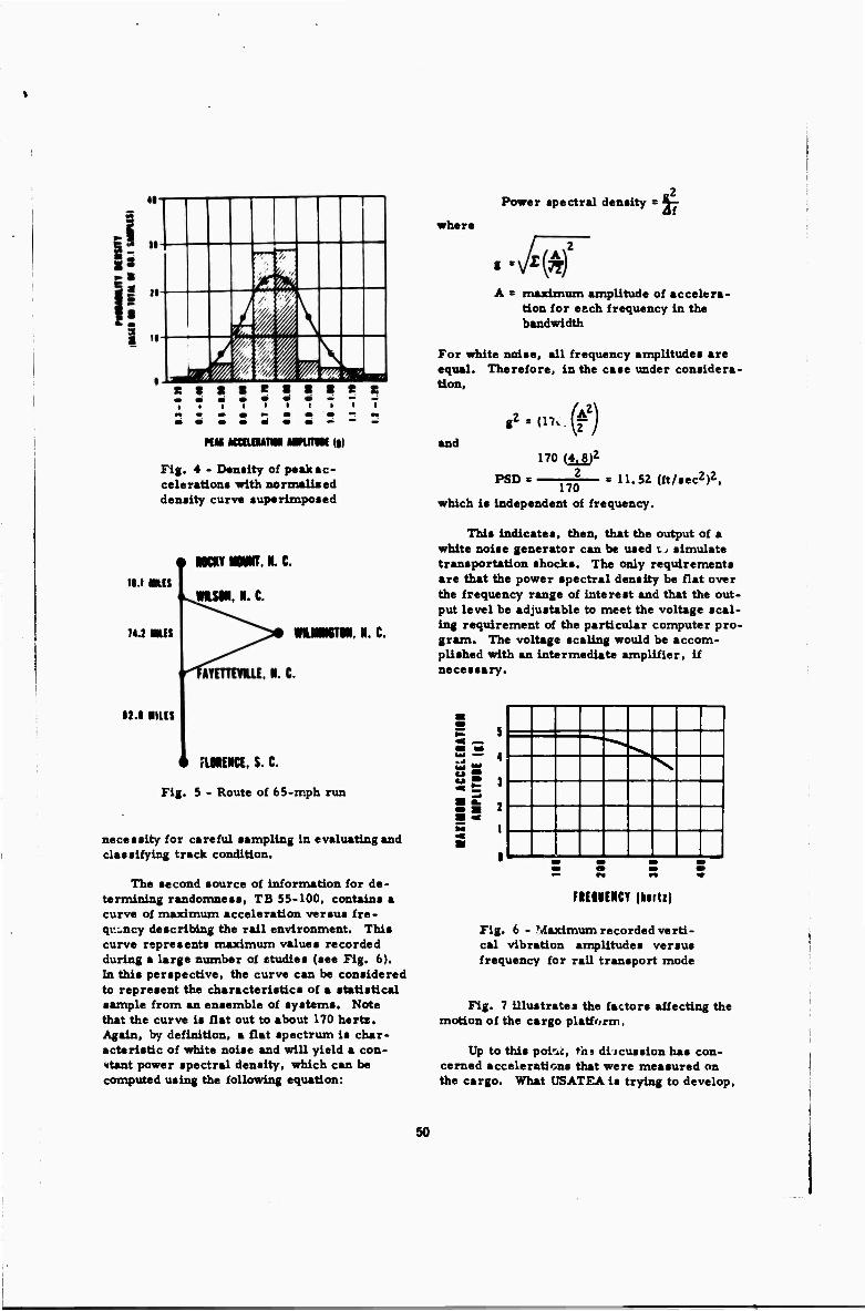
Power spectral density s %-

KM MCtlOMTM twiimt |||

Fig. 4 • Density of peak accelerations with normalized density curve superimposed

II.» WES

9 MCKYMMT.N.C.

■UM. R. C.

I4.J M»

IM IIUS

WIIIMSTN, R. C.

i FLNENCE. S. C.

Fig. 5 - Route of 65-xr.ph run

necessity for careful sampling in evaluating and classifying track condition.

The second source of information for determining randomness, TB 55-100, contains a curve of maximum acceleration versus frequency describing the rail environment. This curve represents maximum values recorded during a large number of studies (see Fig. 6). In this perspective, the curve can be considered to represent the characteristics of a statistical sample from an ensemble of systems. Note that the curve is flat out to about 170 hertz. Again, by definition, a flat spectrum is characteristic of white noise and will yield a con- «tant power spectral density, which can be computed using the following equation:

where

A = maximum amplitude of acceleration for etch frequency in the bandwidth

For white noise, all frequency amplitudes are equal. Therefore, in the case under consideration.

and *■<"-{?)

170 (4.8)2

2 170

which la independent of frequency

PSD = YTQ— = 11.52 (ft/sec2)2.

This indicates, then, that the output of a white noise generator can be used ij simulate transportation shocks. The only requirements are that the power spectral density be flat over the frequency range of interest and that the output level be adjustable to meet the voltage scaling requirement of the particular computer program. The voltage scaling would be accomplished with an intermediate amplifier, if necessary.

FIEIIENCT |kirtt|

Fig. 6 - Maximum recorded vertical vibration amplitudes versus frequency for rail transport mode

Fig. 7 illustrates the factors affecting the motion of the cargo platform.

Up to this poizii, ths discussion has concerned accelerations that were measured on the cargo. What USATEA is trying to develop.

"■"

s

50

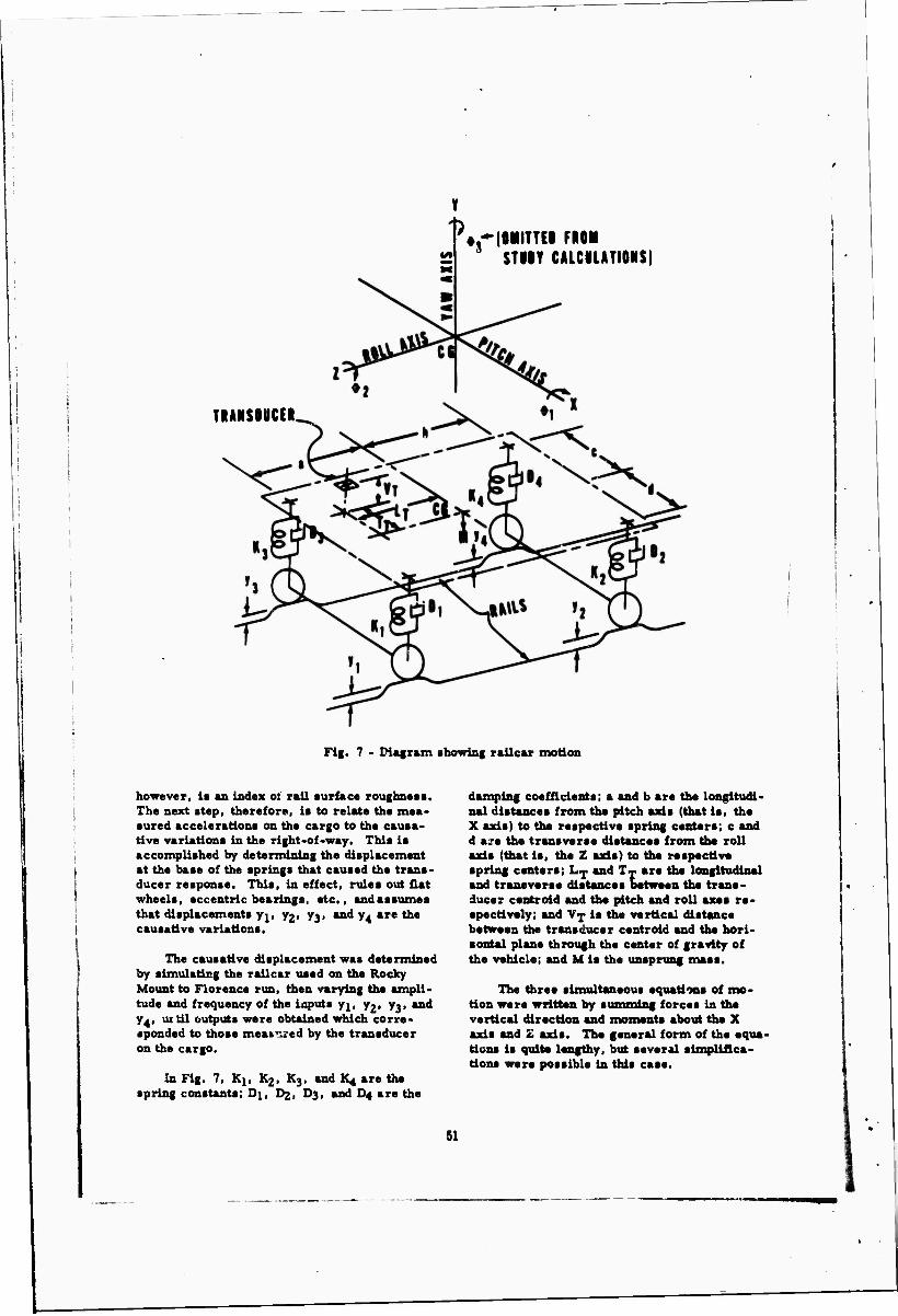
Y

1> ~ ♦,-IOilTTED FROM STIIY CAICILATIONS)

TRANSDUCER

Fig. 7 - Diagram ■howlng rallcar motion

however, la an index of rail surface roughneei. The next step, therefore, la to relate the mea- •ured acceleration! on the cargo to the cauaa- tive variations in the right-of-way. This la accomplished by determining the displacement at the base of the springs that caused the transducer response. This, in effect, rules out flat wheels, eccentric bearings, etc., andassumes that displacements yj, yj. yj, and y^ are the causative variations.

The causative displacement was determined by simulating the rallcar used on the Rocky Mount to Florence run, then varying the amplitude and frequency of the inputs yj, Y2, 73, and y4, until outputs were obtained which corresponded to those meai^red by the transducer on the cargo.

In Fig. 7, Kj, K2, K3, and K4 are the spring constants; Dj, Dj, 03, and O4 are the

damping coefficients; a and b are the longitudinal distances from the pitch axis (that is, the X axis) to the respective spring centers; c and d aje the transverse distances from the roll axis (that is, the Z axis) to the respective spring centers; Lj and Tj are the longitudinal and transverse distances between the transducer ceatroid and the pitch and roll axes respectively; and Vx is the vertical distance between the transducer centroid and the hori- aoatal plane through the center of gravity of the vehicle; and M la the unsprung mass.

The three simultaneous equations of motion were written by summing forces in the vertical direction and moments about the X axis and £ axis. The general form of the equations is quit* lengthy, but several simplifica- tions ware possible in this case.

51

Flg. 8 show* the diagrammatic side and plan views of the loaded car. Note that It is symmetrically loaded. Therefore, the longitudinal and transverse locations of the spring centers with respect to the center of gravity are equal; that Is, distance a is equal to distance b. and distance c is equal to distance d. The spring constants are all equal; that is Kj, Kj, K3, and K4 are equal. Furthermore, it was found that damping could be neglected, thus letting Dj, D2, D3, and D4 equal 0. This process was a safe one for the purpose of developing the index because the ultimate result would be a more severe displacement value for a given roughness description than would have been the case if damping were employed. Since the actual value of the damping coefficient was unknown, this simplification was considered prudent.

Following are the three simplified equations of motion, and a fourth equation relating the motion of the transducer to the motion of the center of gravity:

Y = - § (4Y - yj - y2 - y3 - y4) (1)

YT = Y + Ä'i^T*2 + <VT)2 + (fc)2 (VT) W

In the equations, y is vertical displacement of the center of gravity, and Y is vertical acceleration in feet per second squared; 0j is angular acceleration in pitch in radians per second squared, and ri is radius of gyration about the pitch axis. $2 is angular acceleration in roll, and ri is the radius of gyration about the roll axis.

In equation 4, note that Y is the vertical acceleration of the center of gravity, and Y-j» is the vertical acceleration of the transducer. The computer programming for these equations is straightforward.

Fig. 9 is a block diagram illustrating the method used to simulate the track roughness input.

Since the rail joints On opposite sides of the track are staggered, a compensation was made in the simulation by shifting the inputs on one side of the railcar 90 degrees with respect to the inputs on the other side. This was accomplished by using a sine generator for the two inputs on one side of the car and a cosine generator for the two inputs on the other side.

In addition, the delay between the time the front truck crosses a surface bump at 65 miles per hour and the time the rear truck crosses

VEITICtl KCElEieiETEl

PUN VIE«

SIDE VIE« 11 f 1 !• 1

I

*I3.»"*|*IM"'I' 117"—H

1 1 1

■IM" itr

Fig. 8 - Loaded arrangement of instrumented railcar

52

tmmtmmm nmn HMUTIM rniui h mm*

MM •IHillH

»1 - Miff nut

»IWfWI CMCMI

It

CIWBI IfHIIIM

'1 Ml! mti IIIFtMl (MCIIT

l£

arm iisfociMits It I1SC II SHIMS III

lilfl! ICCIlllltlM ll(l

Fig. 9 - Block diagram for programming vehicle simulation

the same bump can be represented by a phase shift. This is possible because the inputs and responses are steady state. This is expressed by the following equation:

Phase shift (in cycles) = ^~^ x f

where (a+b) = wheelbase in feet

S = speed of railcar in ft/sec f = frequency

A first-order Pade approximation circuit (described in Electronic Associates, Inc., Handbook of Analog Computation^)) wan used to introduce the phase shifts.

A series of 18 runs with different amplitude sinusoidal inputs was made at each of 8 octave intervals between 2 and 256 hertz. Fig. 10 shows traces of the inputs and corresponding outputs at the highest and lowest frequencies studied. The input curves are calibrated in terms of displacement in feet, and the output curves are given in g's.

Fig. 11 shows the family of curves of maximum displacement amplitude at input versus maximum acceleration at the transducer location resulting from the series of computer runs.

Since the slopes of these curves are constant, a simple transfer function is obtained by plotting the ratio of output to input versus frequency.

Fig. 12 is & graph of the transfer coefficient versus frequency. The spike in the graph

/\A/\A A A

-i mm I'Vi

'« |—I/J2 seem—j I

in Inn

t |—i/» seem—|

Fig. 10-2 and 128 hertz inputs with corresponding outputs from railcar simulation

occurs at 4 hertz, which is the natural frequency of bounce of the railcar.

It was found that the dwell time to reach peak acceleration at 4 cycles per second is approximately 1.1 seconds. Dwell times of several cycles were required also with inputs of 8 and 16 cycles before the maximum vehicle response was experienced. Since such dwell times are extremely unlikely to occur in actual operations, and because the graph is remark- ably flat except at the natural bounce frequency, it was considered reasonable to use the mean value of the transfer coefficieut to convert the measured accelerations previously associated with descriptions of ride quality to maximum displacement at the base of the truck springs. As seen on the graph, the mean value of the transfer coefficient is 24g's per foot.

Fig. 13 shows the resulting rail performance index in which are listed five classifications of surface roughness ranging from good to extreme, with corresponding computed values of spring displacement ranging from 0 to 0.2 foot. The values of peak accelerations identified at the end of the loaded test car are shown for comparison with field experience.

Fig. 14 shows a diagram of the instrumentation presently being developed for further studies of the character of surface roughness. An accelerometer is mounted at the base of the springs on one axle of a standard railcar. A resilient mount will be used to eliminate high frequency hash, and the outputs of the accelerometers will be doubly intergrated to provide displacement. Simultaneously, vertical

(^'Electronic Associates, Inc., Handbook of Analog Computation, Princeton, N.J., 1967.

53

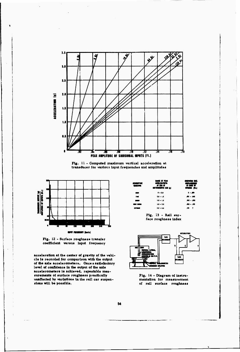
"T* Jl n 11 J! PHI Mnimi IF SIIISIIIIL IWITt |ft.

Fig. 11 - Computed maximum vertical acceleration at transducer for various input frequencies and amplitudes

i t m 1 '"

L

tmmmnu

«I - 1.1

1.1 - i.l

I.I - I.I

1.1 - l.l

Fig. 13 - Rail surface roughness index

Fig. 12 - Surface roughness transfer coefficient versus input frequency

acceleration at the center of gravity of the vehicle Is recorded for comparison with the output of the axle accelerometers. Once a satisfactory level of confidence in the output of the axle accelerometers Is achieved, repeatable measurements of surface roughness practically unaffected by variations in the rail car suspen- sions will be possible.

■«■•«■•■MS

IM MHMI

Fig. 14 - Diagram of instrumentation for measurement of rail surface roughness

54

DISCUSSION Mr. Sonnemann (SlkorBky Alrcrsit): We

have Just completed, as you may know, a fairly extensive work on rail vehicles in connection with our high speed train project. I wanted to comment Just briefly on some of our findings because they do not seem to be in complete agreement with what you stated. We have taken some measurements at the wheel-axle interface in order to determine the rail input due to the discontinuities at the Joints. Frequently, w? have found that we get shocks as high as 20 g and sometimes as high as 50 g. These loads are then rapidly attenuated through the suspension system. Recognizing that it is a passenger vehicle that we are working on compared to the freight car that you were talking about, people's comments as far as a poor ride is concerned would involve levels like 1/2 g. If we exceeded 1/2 g, which we seldom did, people would think the ride was terrible. We have further found that the non-Russian distribution on which you commented is attrib- utable to two factors. One is the poor conditions of curves on the railroad, and the other is the frequency that grade crossings occur. We have seen that the grade crossings will skew the distributions of g-levels a great deal, because it is at this time that the abnormal inputs 3ccur. Tliese become a factor in the skewing. In the light of our own work, I won- der whether your approach can really be representative of rail roughness, because of its nigh dependence on the suspension system. Have you thought about that aspect of it?

Mr. Prothro: We have thought about it. We are aware of the work that you people are doing and we have had the good fortune of being invited to ride your car next week. We plan to do so. One of the things I referred to was the need to develop better sampling techniques. I think this may be reflected in your finding about the distribution being skewed by tra- versing grade crossings. Perhaps the work you have done will be sufficient, but we had hoped to stimulate research in this. I did not know that you had made this discovery.

Mr. Hanks (NASA, Langley): I was won- dering about your indexing procedures including surface irregularities that are much greater in wavelength than the length of the car. It appears in rough calculation that your wavelengths are the approximate length of the car. If your train speeded up to, say, 120 miles per hour then you would not have any idea whether you would encounter this 4 cycle per second roughness or not.

Mr. Prothro: The 4 cycle roughness was

the natural bounce frequency of the car, but the wavelength or the phuse shift that we introduced was baaed on a constant speed of 65 miles per hour. We were comparing this with field data that was made on a constant speed run at 65 miles per hour.

Mr. Hanks: But if you had picked up, say, 1/2 cycle responses or 2 cycles responses these may become critical at 120 or 130 miles per hour. Were you measuring below these levels?

Mr. Prothro: Yes. I guess it was not clear in that diagram but we started with inputs of 2 cycles and even below. We Just diagrammed those octave Intervals starting with 2 cycles. Surprisingly, the responses below that peak range were Instantaneous. In other words, we got the sine wave pattern with an equal amplitude, but in the areas where the peak showed up the responses had to build up. It never did go into uncontrolled resonance.

Mr. Swanscn (MTS Systems): I found this paper extren y interesting because last spring I served as a consultant for British Railways. They are very Interested in the same problems. We characterized the loading that you have as a succession of random processes that the car meets in its history. The interesting thing about it is that each of these bursts is a stationary random process in itself and can be applied in the laboratory as a burst from a random noise generator. In fact they have gone ahead and are now putting in a system which supplies a succession of rms levels.

I would Just like to comment that since your signal is nice and broad-band, It turns out, from sampling theory, that you can get very fast response of your rms level. If you were to put an rms meter on your signal and also filter out the deterministic very low frequency effects like mean load, then you can monitor rms almost instantaneously. I think that your skewing effects and these objective measurements of intensity would go by the board and you could go straight to a nice stable scale of rms's. You could also check for the stretch that you are going to do on probability plots. You could make sure that the values are stationary and that your rms's and constant over that stretch.

Mr. Prothro: I want to point out that our problems occur because someone asks a question. What happens if this thing goes over a rough road? What happens if it goes over a fairly smooth road? We are trying to put a handle on that description.

55

AN APPROXIMATE METHOD OF DYNAMIC ANALYSIS FOR MISSILE CONTAINER SYSTEMS

Mario Paz, Associate Professor University of Louisville, Louisville, Kentucky

and

Ergin Citipitioglu,* Associate Professor University of Louisville, Louisville, Kentucky

♦Present Address: University of Cincinnati, Cincinnati, Ohio

An approximate method of dynamic analysis is presented for missile containers which use elastomeric shock mounts. The missile and its mounting frame are treated as a single rigid body supported by springs and dashpots representing the shock mounts. A parabolic spring rate function is assumed to approximate the frequency dependent dynamic properties of the mounts in the mathematical model. The results obtained by this method of analysis are compared with experimental results for the "Walleye" missile container system.

INTRODUCTION One of the common methods of

protecting missiles from shock and vibration during transportation is to mount the missile carrying cradle (usually a rigid frame) to the container by elastomer type of shock mounts. For approximate dynamic

analysis of this type of missile container , elastomer shock mounts can be idealized by spring and damper systems in three principal directions. The missile toget.ner with the cradle can be treated as a rigid body, thus the whole

FIGURE 1. RESILIENTLY MOUNTED MISSIL!)

57

A

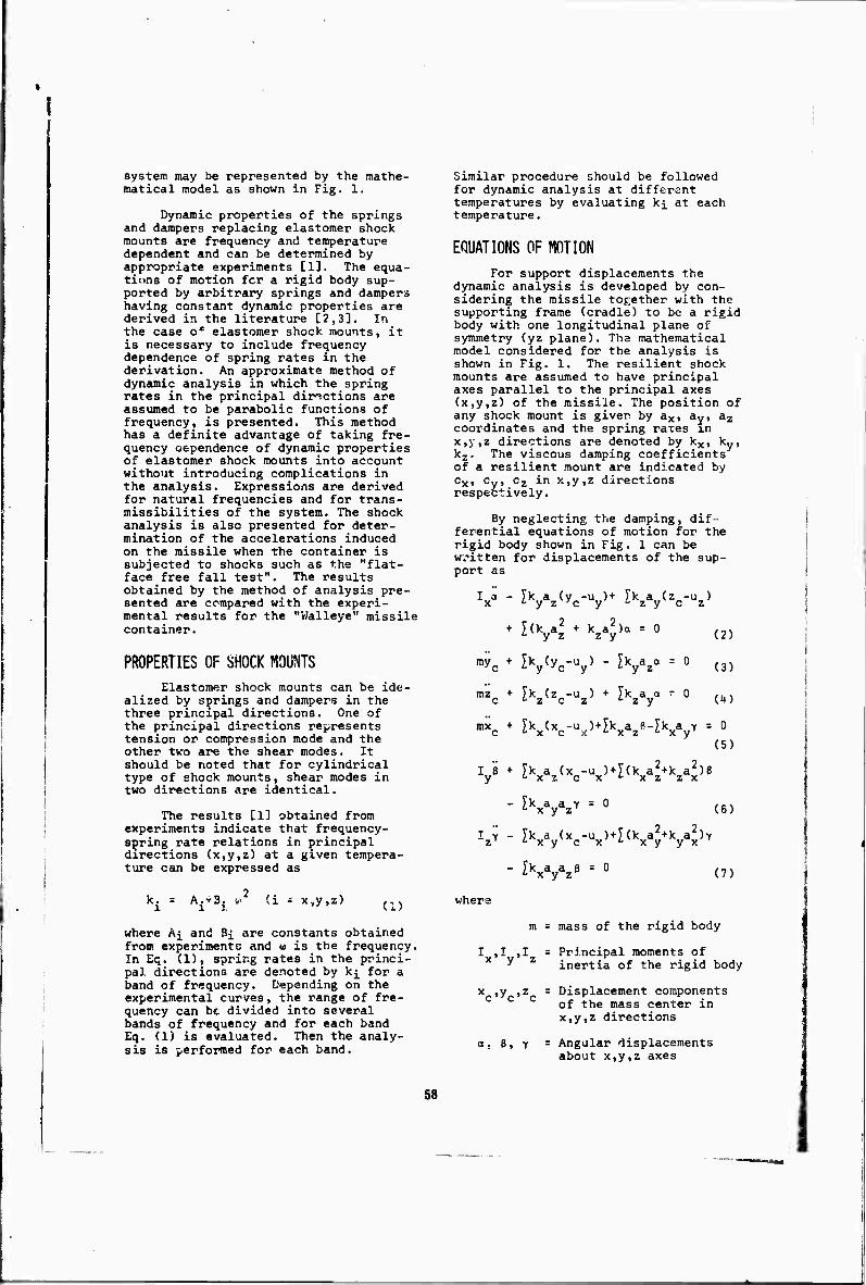
system may be represented by the mathematical model as shown in Fig. 1.

Dynamic properties of the springs and dampers replacing elastomer shock mounts are frequency and temperature dependent and can be determined by appropriate experiments [1]. The equations of motion for a rigid body supported by arbitrary springs and dampers having constant dynamic properties are derived in the literature [2,3], In the case oe elastomer shock mounts, it is necessary to include frequency dependence of spring rates in the derivation. An approximate method of dynamic analysis in which the spring rates in the principal directions are assumed to be parabolic functions of frequency, is presented. This method has a definite advantage of taking frequency aependence of dynamic properties of elastomer shock mounts into account without introducing complications in the analysis. Expressions are derived for natural frequencies and for transmissibilities of the system. The shock analysis is also presented for determination of the accelerations induced on the missile when the container is subjected to shocks such as the "flat- face free fall test". The results obtained by the method of analysis presented are compared with the experimental results for the "Walleye" missile container.

PROPERTIES OF SHOCK MOUNTS Elastomer shock mounts can be ide-

alized by springs and dampers in the three principal directions. One of the principal directions re-presents tension or compression mode and the other two are the shear modes. It should be noted that for cylindrical type of shock mounts, shear modes in two directions are identical.

The results [1] obtained from experiments indicate that frequency- spring rate relations in principal directions (x,y,z) at a given temperature can be expressed as

Similar procedure should be followed for dynamic analysis at different temperatures by evaluating ki at each temperature.

EQUATIONS OF MOTION For support displacements the

dynamic analysis is developed by considering the missile together with the supporting frame (cradle) to be a rigid body with one longitudinal plane of symmetry (yz plane). Tha mathematical model considered for the analysis is shown in Fig. 1. The resilient shock mounts are assumed to have principal axes parallel to the principal axes {x,y,z) of the missile. The position of any shock mount is given by ay, ay, a2 coordinates and the spring rates in x,y,z directions are denoted by kx, ky, kz. The viscous damping coefficients of a resilient mount are indicated by cx, Cy, c2 in x,y,z directions respectively.

By neglecting the damping, differential equations of motion for the rigid body shown in Fig. 1 can be written for displacements of the support as

V - Ikyaz(yc-Uy)+ ^zVVV + SV*+ kza5)a - °

myc + IVyc-V ' ^Vza = 0

mzc + ^VVV + ^kzV r 0

(2)

(3)

(4)

+ Ikx(xc-ux) + Ikxaz6-^xV = 0

(5)

V + Kaz(xc-ux) + I(kxaz+kzax)ß

ZVyV = 0 (6)

I Y - Vk a (x -u )+y(k a2+k a2)Y z L x y c x *• x y yx

" Ikxayazß = 0 (7)

k. = A.T3. 1 13.

(i - x,y,z) (1)

where A^ and Bi are constants obtained from experiments and u is the frequency. In Eq. (1), spring rates in the principal directions are denoted by k^ for a band of frequency. Depending on the experimental curves, the range of frequency can be divided into several bands of frequency and for each band Eq. (I) is evaluated. Then the analysis is performed for each band.

where

m = mass of the rigid body

I ,1 ,1 = Principal moments of ^ inertia of the rigid body

x ,y ,z - Displacement components of the mass center in

B. Y

x,y,z directions

Angular displacements about x,y,z axes

58

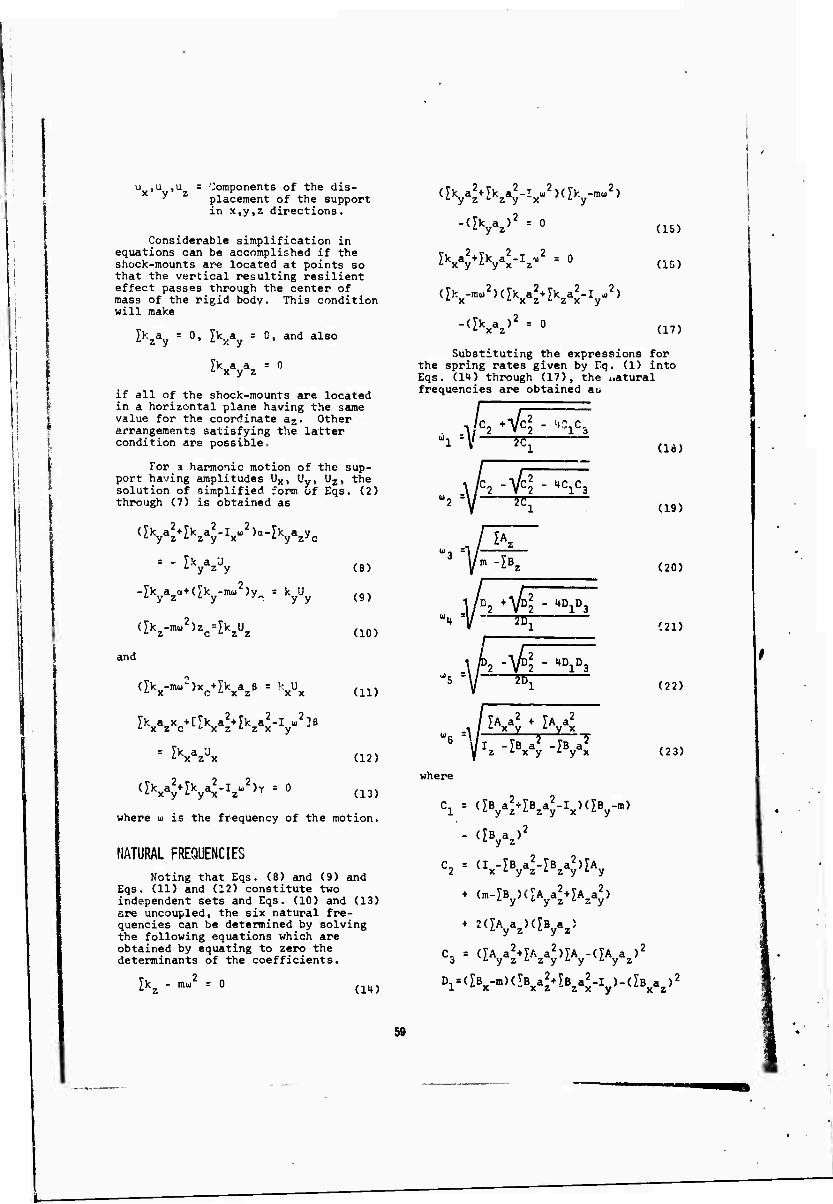
u ,u ,u = Oomponents of the dis- " placement of the support

in x,y,2 directions.

Considerable simplification in equations can be accomplished if the shock-mounts are located at points so that the vertical resulting resilient effect passes through the center of mass of the rigid body. This condition will make

J>zay = 0, l\Ay - 0, and also

l>xa..a y z 0

if all of the shock-mounts are located in a horizontal plane having the same value for the coordinate az. Other arrangements satisfying the latter condition are possible=

For a harmonic motion of the support having amplitudes Ux> Uy, Uz, the solution of simplified form of Eqs. (2) through (7) is obtained as

y z ^ z y x

= - 5> a"J i y z y

y z'c

-Tk aa+(/"k -mu )y = k U tyZ ty -'•-; yy

(lk-mu2)z -^,0, L z c L z z

and

(Ikx-mu2)xc+Ikxazß = kxUx

- ^xazUx

(8)

(9)

(10)

(11)

(12)

(13)

where u is the frequency of the motion.

NATURAL FREQUENCIES Noting that Eqs. (8) and (9) and

Eqs. (11) and (12) constitute two independent sets and Eqs. (10) and (13) are uncoupled, the six natural frequencies can be determined by solving the following equations which are obtained by equating to zero the determinants of the coefficients.

(^yaz+Ikzay-Ixu2)(Iky-mu2)

-(Ikyaz)2 = 0

£Vy+Vx-V2 ' 0

([kx-mu2)(Ikxa**IkzaJ-V

2)

-(Ikxa2)2 = 0

(15)

(IG)

(17)

Substituting the expressions for the spring rates given by Tq. (1) into Eqs. (lU) through (17), the ..atural frequencies are obtained au

*isV k +,^r ^ic

3

^i /

h -vl ■ *€&

i 2ci

[A L y

U -IB,

,l/D2 "VD2 --D1D3 7 " gBl

, JA a2 + [A a2 =W ^ x y / y x

6 "'l -IB a2 -IB a7 z i x y L y x

where

(10)

(19)

(20)

(21)

(22)

(23)

Ik, - mu = 0 (II»)

Ci = (lBya^lBzaJ-Ix)(lBy-m)

C2 = <l*-l*y4-l*z*PlAy * (m-lBy)(lAya

2+lAzaJ)

+ 2aAya2)(lByaa)

S = (lAya2+lAzaJ)lAy-(lAyaz)

2

D1=(lBx-m)(lBxa2^Bza

2-Iy)-(lBxaz)2

59

+ (m-TBx)(lAxa^lAzaJ)

+2{lAxaz)(lBxa2)

D3 = (lAx){lAxa^lAza2)-(lAxaz)2

TRANSMISSIBILITIES Damping can easily be introduced

in Eqs. (9) through (13) by substituting ki+jwc- for k£ where j is imaginary unit and subscript i indicates x, y, and z. Ther\ after introducing damping, the transmissibilities are obtained for a forced frequency n by solving Eqs. (8) through (13) as

,2r , ,r, N2ir,2

the natural period of the system. Impulse results in an instantaneous change of velocity, after which the system starts a motion characterized by free vibrations. Therefore, shock tests may be simulated analytically by free vibrations of the missile with an initial velocity du2 to stipulated conditions. Analytical studies [2] ir-dicate that the effect of damping in the maximum acceleration resulting from shock is relatively small, therefore it is neglected in the following analysis.

The differential equations of motion (Eqs. (2) through (7)) are solved for an arbitrary initial velocity

*:' t^V" KV(£kxV +" 'KV^ +[IkxnV"A5K-^(^xaz)(^xaz)]

n 1/2

2

,2.„2, T

c

CV5-"'KA6-(^xV +fl'(KV ] +[A4nA6+nA5Icx-2fi(Ikxaz)(Icxaz)]'

2 [Ajk -sTAjc -(Tk ajWcTc a r] ♦CA,«^ ♦Ajk ö-2n(Jk a )<Ic„a,)]' I'-y 2L y L w z L y z lLy2'-y '■yz'-yz

[A1A3-fi2A2Icy-(Ikyaz)2

+n2(Icyaz>2] +[AlnIcy+A2A3n-2fi(Ikyaz)(Icyaz)]'

1/2

(24)

1/2

(25)

(I^)2+n2<K)2

5 (Tk -mf!2) +n2(yc,)2

y z . (26)

where

A, = Tk a2+yk a2-I a2

1 L y z ^ z y x

A2 -- 1^1*1^1

A, = Tk -mn 3 L y

\ -- IV'nn2

A,. = Jk a2 + yk a2-I n2

5 '■xz^zx y

A6 = Icxaz^czax

SHOCK ANALYSIS Specifications O] for missile

mounting limit the acceleration of the missiles when the system is subjected to stipulated shocks. Dynamically, a shock is an impulsive force acting in a short duration of time compared to

by making u , u , u equal to zero. The resulting expressions for the angular motion of the rigid body and for the linear displacements of the mass center are given by Eqs. (27) through (32).

a = c-sinu.t+c-sinu.t

y - R,c., sinu, t+R-c-sinu-t c ii 1 it i

z = c-sinu-t Co i

x = c^sinu.t+c-sinuct

B = RjC.sinui^t+R^CrSinurt

Y - c-siniu.t

(27)

(28)

(29)

(30)

(31)

(32)

where

RTa„-y^ ym"Ria^ 2 o Jo o lo u^R^-R,) ' C2 = STTRT^O

60

o

go-R3xo

-5(%-R3) ' C6

Jk a^Jk a2-I u? L y z L z y x 1

Jk a ^ y z

R {o-6o spring rates corresponding to natural frequencies u,, u?, or uu, w, is relatively large, the error may become unacceptable.

Now, the procedure for shock analysis can be outlined as follows:

1. Determine the components of the initial velocity from the shock test under consideration. (This step is discussed in Ref. [1])

[k af+Jk a -I u, R - y z z y x 2 2 Jk a

<■ y Z

R3 =

[k -n U v

Jk a L x z \ -

^V^5 Ik a ^ x z

2. Compute the coefficients for Eqs. (27) through (38).

3. Since the expressions obtained in step 2 are for the mass center, maximum linear accelerations can be computed by evaluating the accelerations at various points of the missile.

and

a ,8 ,Y = Initial angular velocity of the rigid body about x,y,z axes.

x„»y„»z„ s Initial linear velocity ooo , ,. . _ xn x.y.z directions of the mass center.

M, ,u. ju,,«^ ,uj ,(iig = Natural frequencies from Eqs. (18) through (23).

By differentiating Eqs. (27) through (32) witn respect to time twice, the expressions for angular acceleration of the rigid body and for the linear accelerations of the mass center are obtained as

a r -c1ull sinu^t-Cj«2 sinu.2t (335

"2 2 y s ""i0!"! sinu.t-RjC-u- sinu.t

zcz "c3",3 Slnu3t

(3U)

(35)

APPROXIMATE DYNAMIC ANALYSIS FOR "WALLEYE' MISSILE CONTAINER

A schematic diagram of the "Walleye" missile container system is shown in Fig. 2. The locations of the mass center (eg) and ahock mounts are indicated along with other pertinent dimensions. Data regarding the missile and container were provided by U.S. Naval Ordnance Station, Louisville, Kentucky.

NUMERICAL DATA 2

Mass Moment of Inertias (slug-ft )

I = 233.0; I = 7.80; I = 233.0 x ' y ' z

Weight of the Missile and Cradle (lbs.)

Weight of the missile W = 1100

Approximate weight of cradle W = 100

Total weight mounted

PROPERTIES OF SHOCK MOUNTS

W = 1200 m

V -c^l sim^t-CgUg sinu^t (36)

-R3CUUU sinu4t-c5RUu5 sinuit

(37)

Lord Company type J-5682 shock mounts were used. Experimental prop- erty values at ambient temperature as given in the appendix of Ref. [1] are:

Spring Rates (lb/in)

-CgUg sin«6t (38)

It should be noted that Eqs. (27) through (38) are approximate due to the fact that spring rates are frequency dependent. If the change in

For compression k =3065.'♦8+0 .0368«

k sk =789+0.068«' y z

For shear

where u is frequency in radians/sec.

61

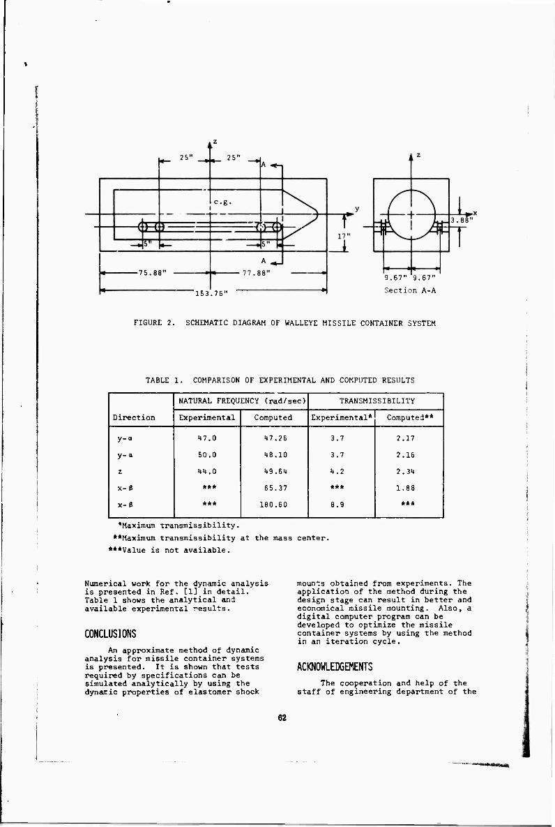
153.76"

9.67" 9.67"

Section A-A

FIGURE 2. SCHEMATIC DIAGRAM OF WALLEYE MISSILE CONTAINER SYSTEM

TABLE 1. COMPARISON OF EXPERIMENTAL AND COMPUTED RESULTS

Direction

NATURAL FREQUENCY (rad/sec) TRANSMISSIBILITY 1

Experimental Computed Experimental* Computed**

y-a

y-a

z

x-B

x-e

47.0

50.0

44.0

***

***

47.26

48.10

49.64

65.37

180.60

3.7

3.7

4.2

***

8.9

2.17

2.16

2.34

1.88 j

***

♦Maximum transmissibility. **Haximum transmissibility at the mass center.

***Value is not available.

Numerical work for the dynamic analysis is presented in Ref. [1] in detail. Table 1 shows the analytical and available experimental results.

CONCLUSIONS An approximate method of dynamic

analysis for missile container systems is presented. It is shown that tests required by specifications can be simulated analytically by using the dynaric properties of elastomer shock

mounts obtained from experiments. The application of the method during the design stage can result in better and economical missile mounting. Also, a digital computer program can be developed to optimize the missile container systems by using the method in an iteration cycle.

ACKNOWLEDGEMENTS The cooperation and help of the

staff of engineering department of the

62

1

U.S. Naval Ordnance Station, Louisville, Kentucky and of Dr. I.W. Tucker, Director of University of Louisville Institute of Industrial Research is acknowledged.

REFERENCES 1. Paz, M. and Cilipitioglu, E., "Manual for Missile Mounting" Report, prepared for Naval Orünance Station, Louisville, Kentucky, Dec. 1966.

2. Harris, CM. and Crede, C.E. (Editors), Shock and Vibration Handbook, Vol 1, 2, 3, McGraw-Hill, New York, 1961.

3. Meriam, J.L., Dynamics, John Wiley and Sons, Inc., New York, 1966.

U. "Design and Test of Packaging, Packing, Shipping and Handling Equipment for Weapon System Components", Bureau of Naval Weapons, Department of Navy, WR11, July 1963.

DISCUSSION

Mr. Seely (Naval Ordnance Station, Forest Park, 111.): You showed a slide showing a nat-~ ural frequency of about 47 Hertz for your container. It may interest you to know that I have just tested a Walleye container and the natural frequency came out to somewhere between 9 and 11 Hertz. The transmlsslbllity ran about 5.

Mr. Cltlpltloglu: This is radians per second hereT

Mr. Seely: That does make a difference.

Mr. Linton (Naval Weapons Station. Seal Beach): We do vibration and shock testing of containers of various sorts up to perhaps 16 leet long weighing a couple of thousand pounds. On the vibration tests we are asked to find the resonant frequency and dwell there. We often find no definable resonance. Perhaps more particularly, they seem to resonate at any frequency up and down the line. This leaves the thought that the larger containers do not seem to have the spring mass system as precisely defined as your analysis Indicates for your Wall- eye container. In trying to do a valid test, it is often difficult to find these resonant frequencies due to the resonances in the container. These are long flimsy containers that shake like a bowl full of jelly at any frequency.

Mr. Cltipitloglu: We have not tested the Walleye container. We only used the test results which were available to us. From the mathematical analysis under the assumptions that we have, It Is clear that we must have some kind of natural frequency. For the kind of missile containers you are talking about I am not sure what the range of the frequency will be.

Mr. Griffith (Bendlx Missiles System Dlv.): We have designed and built containers for one

of the Navy's larger complete weapons system. We also did some testing for the Naval Ord- nance Plant at Louisville on a container which I think was for the Walleye. Contrary to what the gentlemen from Seal Beach Just said, we have never experienced any problem In determining the resonance of the container suspen- «ica system. Our particular weapon has a spring damper system. At resonance we found out we could burn out the dampers very easily because of the motion in there. I think the Walleye container that we tested had some resonances which had transmisslbilities around 11 or 12. This is a pretty solid resonance and you should find it easily.

Mr. Cltipitloglu: I am familiar with the type of missile container that has dampers on it, but the type on which we worked was strictly mounted by elastomer shock mounts. We did not make any study of the type that you mention.

Mr. Matthews (Naval Missile Center): I tested a shipping container many years ago and found that there are occasions when you can find a resonance and other occasions when you cannot. It depends on what the cushioning material is. If it is linear, of course, you will find a resonance, but many of these things have elastomers and if you study the stress strain curves you will find them very nonlinear. Now if you try to test these to a specification that says find the resonance and dwell there for an hour, then increase the level of your input and dwell there for an hour you will find that you will have a different "resonance.* Also, you will find that the resonance will shift as you dwell there because the temperature affects the nonlinear behavior. I re»Uy think that the concept of a resonance and a dwell for these nonlinear cushions has to be looked at very carefully. I

SIHUUTED MECHANICAL IWACT TEST EQU1P«NT

D. R. Agnew

Naval Air Developnent Center Johnsvllle, Wamlnster, Pennsylvania

A unique test method has been developed to determine the structural integrity of unit shipping containers for "A"-size stores when subjected to lateral lapacts. To facilitate reproducibillty of test, control of Impact and ease of handling in the perforaance of this test method, the Simulated Mechanical lapact Test EauiDaent (SMITE) was designed, developed and found to be satisfactory and practical.

INTRODUCTION

A unique test method has been developed to determine the structural integrity of unit shipping containers for Navy stores when subjected to lateral Impacts. To facilitate reproducibillty of test, control of impact and ease of handling in the performance of this test method, the Simulated Mechanical Impact Test Equipment was designed, developed and found to be a satisfactory and practical test facility.

The need for such an apparatus became apparent about two years ago when damage reports were submitted to the Aero Materials Department Indicating that unit shipping containers used for the packaging of Navy "A"-slze stores were unsatisfactory. In- vestigations of these reports disclosed that the current plastic shipping containers flex under Impact and allow the "A"-slze stores to be dented without any visible damage to the shipping container. These "A"-slze stores are basically rugged electronic hardware which can take high "C" forces but once the thin outer aluminum skin is dented, there is a high obability of a malfunction in performance due to the internal electronic components becoming damaged or "hung-up" and not being properly deployed for operation.

Further examinations of these damage reports revealed that after a 700-mile trip by commercial carrier, the electronic hardware experienced typical damage as depicted in Figure 1. This damaged hardware was reported as inoperable.

In simulating the type of damage reported, the unit containers with hardware were banded four together as prepared for shipment and

subjected to the various types of lapacts e.g., the tlpover onto a pallet. Impact onto a loading platform and impact onto a truck bad. In all instances, the impact tests were difficult to accomplish du« to the bulk of the pack, weight of the pack and the variance In the human factor. By this variance In human factor, it is meant that In simulating hefting of the pack onto a truck bad or loading platform, it was found that the sic« and physical condition of the person performing the test were contributing factors in the outcome of the tests. Between the types of impact tests attempted, the tlpover onto a pallet (Figure 2) was the easiest to perform and just as severe as the others.

Though the tlpover test was the least difficult to perform, problems were still encountered:

1. The test pack as prepared for shipment can weigh up to 125 lbs. and thus requiring at least two test mechanics to perform the tests.

2. The actual tipping over of a pack this size is an unwieldy process and very often more than one specimen may be damaged in the drop test, or multiple test drops may have to be performed to Insure reproducibillty of results.

To eliminate these difficulties, it wee attempted to:

1. Reduce the test personnel to one by applying the force of impact of a shipping pack tlpover to a single container sample and thus reducing the specimen weight to be handled.

2. Position the container as depicted in

65

I

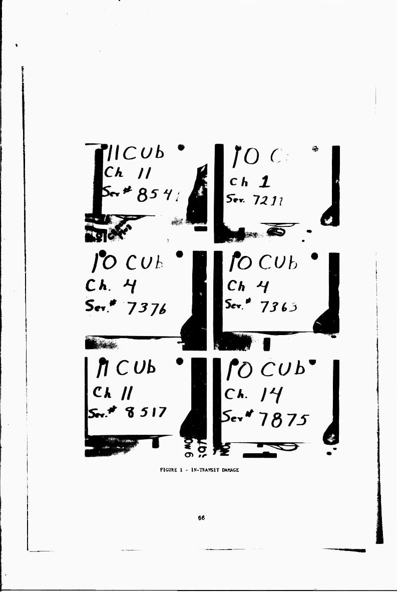
FIGURE 1 - IN-TRANSIT DAMAGE

66

FIGURE 2 - TIPOVER IMPACT ONTO A PALLET

67

Figure 3 and allow the equivalent tlpover Ira- pact force of a shipping pack to fall verti- cally onto the container »ample.

3. Achieve optimum control of the test procedure by mechanizing all the dynamic parameters of the test method.

The solution to all these difficulties resulted in the design and development of tl,4 Simulated Mechanical Impact Test Equipment, Figures 6 and 5, which produces damage equivalent to a shipping pack tipping over, represented by a single unit container. Figure 6.

In determining the test method parameters and designing the SMITE, it «as necessary to conduct the extensive mathematical study that follows:

A derivation relating the rotational parameter* of a two-container pack tipping tandem onto a pallet edge to the vertical parameters necessary to give equivalent motion and force during a free-fall drop is presented.

1. The moment of inertia of a right circular cylinder (length • R, radius > r and Mass • M) shall be calculated with respect to its geometric and gravity centers which are one and the same in this case. This cylinder is to be representative of a unit shipping container for Sice "A" stores. Monent of inertia of a solid circular cylinder about an axis through the center of gravity and perpendicular to the axis of the cylinder is:

Z

it 12

Bxolanatlon: Moment of inertia with respect to the perpendicular plane is Ixy ♦ Ixz • Ix

Ixy » kMr% r » radius

Ixz > I ML2, L • length (R) 3 but at CG. L > R

2 2

2. This previous equation (Ix) suggests the shipping container rotates around its center of gravity like a pin wheel, ileh is not indicative of a tipping-over process. The pivot point for the tlpover is contained In the bottom of the upright container and, therefore, I (Ixj) In the base of the container must be found.

Now consider I of an axis (xj) in the base of the cylinder and parallel to the axis (x) through the CG. which was used in the calculation of Ix as described above.

Z

O.

,/ /

.'

^

I

/

/

Parallel-axis theorem for masses:

I » T + Md2; but d - R 2

Ix. - Ix + M R2

4

Ix. - M .r2 ^ R2 >■> MR2

* 12 ' 4

Ix. • M .r£ * R£ , A3

3. Again, this last equation (Ixj) is not wholly indicative of a shipping pack tipping. In actuality, the effective impact Is that of & two-unit container, in tandem, striking a pallet edge while pivoting about a point (P) In the base. Therefore, the moment dp) of two-unit containers rotating about a point (P) must be found.

Now consider two cylinders placed together:

.'.I« kMrz ♦ 1 Ml/ 3

kMr2 ♦ I HI2

12

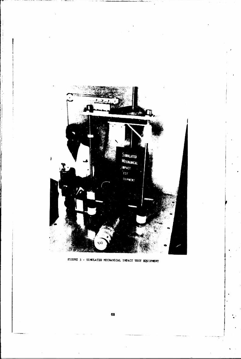
FIGURE 3 - SIMULATED MECHANICAL IMPACT TEST EQUIPMENT

60

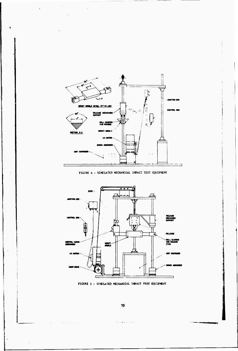
FIGURE It - SIMULATED MECHANICAL IMPACT TEST EQUIPMENT

FIGURE 5 - SIMUUTED MECHANICAL I»ACT TEST BQUIP«NT

70

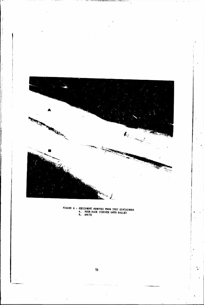
^vJ

FIGURE 6 - EQUIPMENT REMOVED FROM TEST CONTAINERS A. POUR-PACK TIPOVER ONTO PALLET B. SMITE

71

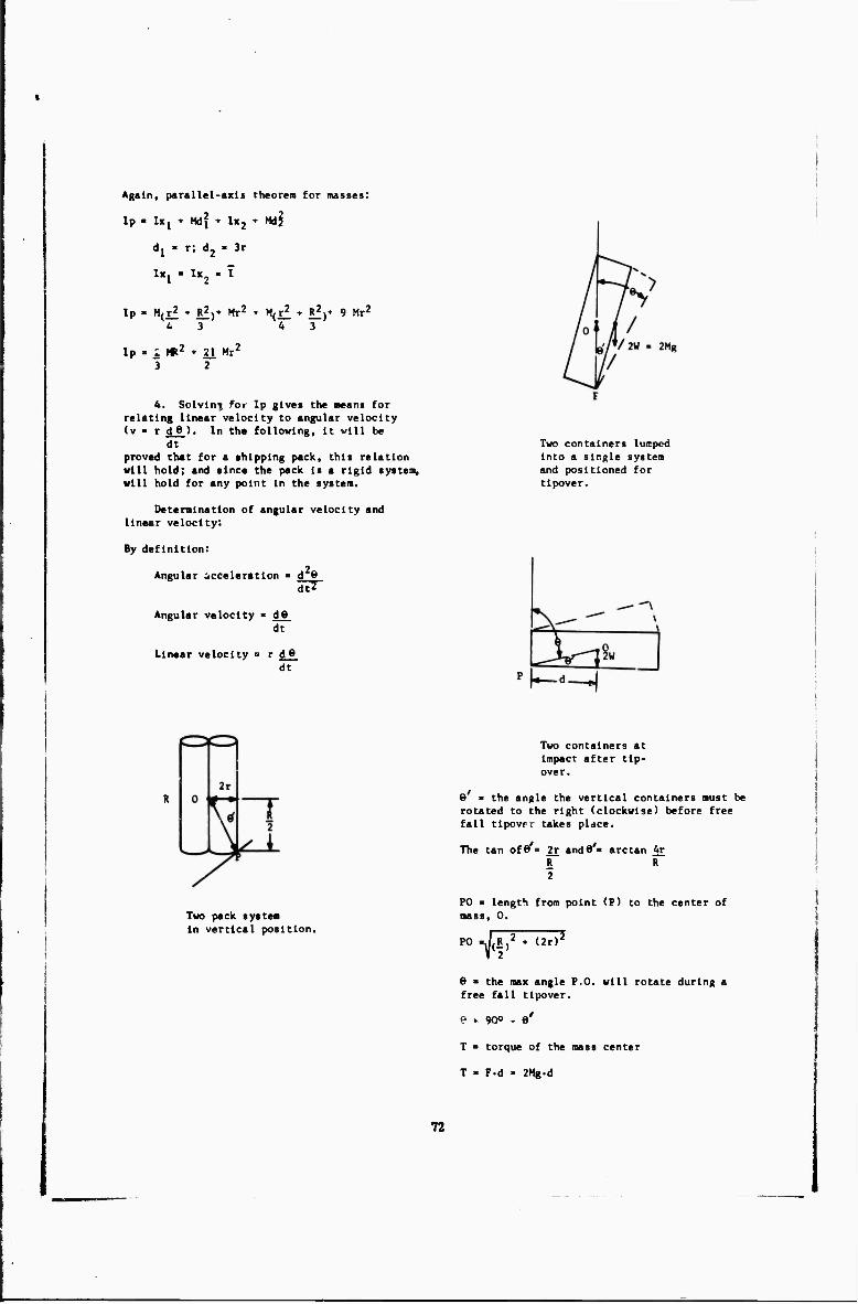
Again, parallel-axis theorem for masses:

Ip • IKJ * m* " lx2 » mj

dj • r; d, - 3r

lx1 - 1K2 - T

Ip ■ M(r£ ♦ R^)* Mr2 ' M(r£ ♦ R^)* 9 Mr2

6 3 4 3

Ip - i «2 » 21 Mr2

4. Solvlni for Ip gives the means for relating linear velocity to angular velocity (v • r de ). In the following, it will be

dt proved that for a shipping pack, this relation will hold; and since the pack is a rigid system, will hold for any point in the system.

Determination of angular velocity and linear velocity:

By definition:

2 Angular acceleration « d 9

dtZ

Angular velocity ■ d8_ dt

Linear velocity ° r d 8 dt

Two containers lucpcd into a single system and positioned for tlpover.

Two pack system in vertical position.

Two containers at Impact after tipover.

6 • the angle the vertical containers must be rotated to the right (clockwise) before free fall tlpover takes place.

The tan of* » 2r andfl'« arctan 4r R R 2

PO « length from point (P) to the center of mass, 0.

PO -fr 2 ♦ (2r)2

6 « the max angle P.O. will rotate during a free fall tlpover.

« » 90° - e'

T > torque of the mass center

T • F-d - 2Mg.d

72

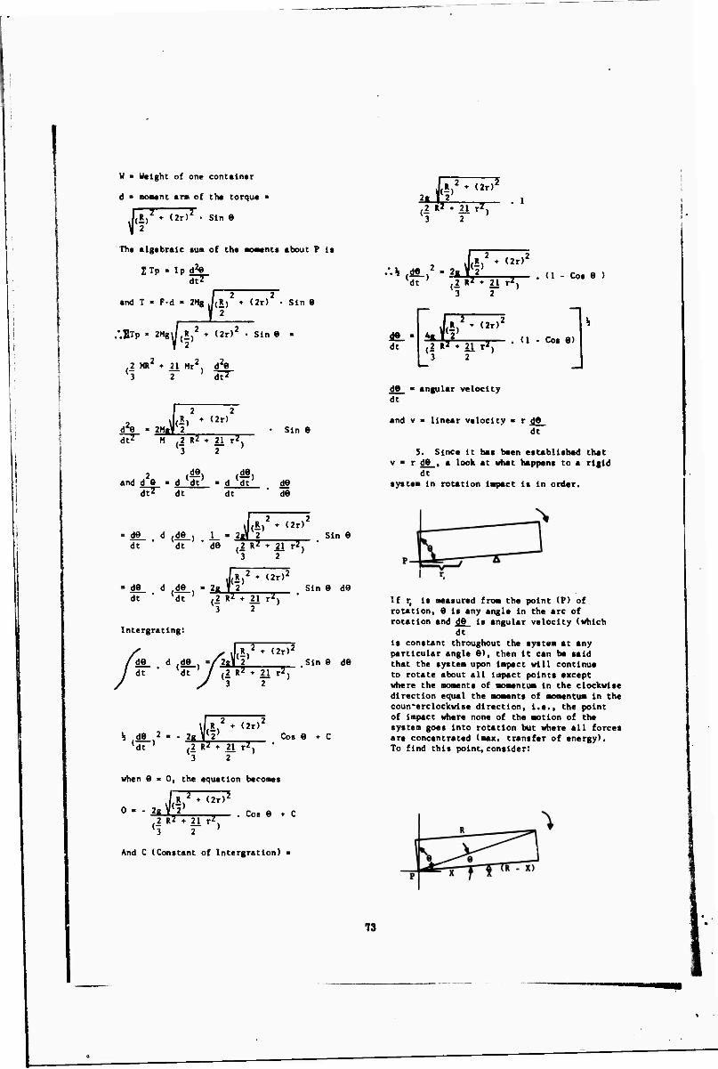
W • Weight of one container

d * monent am of the torque •

I (R,2 ♦ (2r)Z • Sin 6

The algebraic sun of the aoaenti about P 1*

JTp . Ip d2» dtZ

and T » F-d • 2Mg ^(R)2 ♦ (

V'f'

2r) • Sin 9

'.jTp ' 2Mgi/ R 2 » (2r)2 • Sin • -

2 MR2 ♦ 21 Mr2, d2» *3 2 dt^

d2» - 2Ma' j(|) - (2r)

dt' M 2 R2 ♦ 21 rz, 3 2

2 (^) (dS) and d 9 « d dt - d dt

dtz dt dt

Sin 6

d« d«

IIT^2^ c ri 2 Sin de d jdfL, J_ • 2rf ___, dt " dt ' de .2 RZ » 21 r2,

3 2

j(l)2 T «2r)2

de d de_ » 2g r2 dt " (dt ' {2 R2 ♦ 21 r2)

sin e de

Intergrating:

/ I R * (2r)2

de d .de_. '/izvV ,sin e de dt ■ At J (2 Rz ♦ 21 r2) "

l/ R 2 ♦ (2r)2

^ ^de. 2 • - 2» vy cos e ♦ c (dt ' ,2 RZ + 21 rZ, '

3 2

when 8=0, the equation becomes

i*,2 + <2^2 o ■ - zgYz' . cos e + c

2 RZ + 21 rZ l3 2 '

And C (Constant of Intergratlon) «

JF (2r)'

.2 RZ ♦ 21 r2

3 f M

•••% d. 2.2.Ji>r7^ Cos e )

dt KL (2r)'

,2 RZ ♦ 21 rZ (1 - Cos e)

2

de » angular velocity dt

and v ■ linear velocity ■ r dfl dt

S. Since It ha« been established that v ■ r de . a look at what happens Co a rigid

dt «ysten in rotation lapact Is In order.

If r, Is measured froa the point (P) of rotation, 9 is any angle In the arc of rotation and de Is angular velocity (which

dt Is constant throughout the «ysten at any particular angle e), than it can be said that the systen upon Inpact will continue to rotate about all Impact points except where the moments of nomentun in the Clockwise direction equal the moments of aonantua in the coun'erclockwlse direction, i.e., the point of impact where none of the motion of the system goes into rotation but where all force« are concentrated (max. transfer of energy). To find this point, consider:

73

Point X is to be the lapact point of aax. transfer of energy and, therefore, no new rotation ii caused (X Is measured along the container wail). Forces to the right of the lapact point will tend to cause a clockwise ■oticn and forces to the left will tend to cause counterclockwise notion. Therefore, the effective uss in the counterclockwise

direction would be X 2M, (2M being the mass R "

of two unit containers in tandem) which acts at a center of mass of T'= X from the impact

2 point and with v'« T'M tr', measured from

dt P, equals X); the solution for the moment of

2 entum in the counterclockwise direction is:

■'v'lj'-jX (2M)) (X d»,, (X) R * 2 dt ' 2

M_ 2R

d«

dt

Then it can be stated that the point of maximum transfer of energy on Impact and the point where none of the motion of the system goes into rotation on impact is 0,62 the length of the container (0.62R).

6. Now equating linear nomentums to angular momentum

2 MV (linear) - 2Hr d» Cangular) dt

from (4) d* •

dt *£ (2r)' 2 R^ - 21 r-1

3 2

(I • Cos 8)

from (5) r = 0.62R

.•.2MV - 2M (0.62R) JL (ar)4

2 Rz » 21 rz

3 2

(1 - Cos 8)

The effective mass in the clockwise direction would be R - X 2M which acts «t

■" R- *

a center of mass t;*» R - X from the impact 2

point and with v'» jfM (r'measured from p dt

equals R ■> X); the solution for the moment of 2

momentum in the clockwise direction Is:

n'v*^ R - X (2M). .R -^ X d« ) (R - X)

2 * 2 dt * 2

M_ d« (R + X) (R 2R • dt

X)'

which Is the effective momentum at the maximum transfer of energy at point of impact for a two container system tipping over in tandem.

Again, equating linear momentum to angular

M1V 2M - d8 dt

M -figs = 2M (0.62R)

JL: (2rr

TRTTTr7" 3 2

(1 • Cos 0)

As previously stated when the moment of momentum in the clockwise direction equals the moment of momentum in the counterclockwise, none of the motion of the system goes into rotation but is concentrated at the impact point; therefore.

and M

M_ 2R

d« dt

M_ d» (R + X) (R - X) 2R * dt '

7. From (6), it can be said the vertical parameters necessary to give equivalent motion and force during a free fall drop are now equated to the rotational parameters of a two container pack tipping tandem onto a pallet edge 5" high.

M V . 2M r d» 1 dt

expanding

X3 • (R ♦ X) (R - X)2

XR" 2X2 R » X3 ^ RX2 - R3 2XR'

X3 • R3 - X2 R

0 • R3 - X2 R

XR'

XR'

0 • -R (X2 ♦ XR - R2)

Solving for X give* a positive root at 0.62 R.

V^ V^gs = 2W2 (0.62R)

g ' 8

r 4*2' (1

.1R.2 + (2r)2

2 Rz + 21 r2 Cos 9)

3 2

Wj > Weight of free falling body

W. • Weight of unit tipping over plus weight of container

74

g » Acceleration due to gravity

R « Length of pack

r > radius or half the width of a unit container

0 « 90° - arctan Ar - arciln _5 R .62R

From this equation, a solution for S can be found, which is the distance the impact missile of the SMITE should be dropped onto the unit container to simulate the most severe rough handling environment that this particular type ot shipping container will experience.

Currently, the SMITE is required by specification MIL-S-23665 as one of the major procedures for preproductlon testing of unit shipping containers covered by that s;-eclfl- cacion.

So far, this presentation has dealt with more or less a specific packaging problem whereas it Is becoming more evident that many packaging systems are being damaged by the same types of impacts as described here. Further, it has been observed that shipping containers have received other types of lateral Impacts whether from fork lifts, containers banging Into one another, ramming Into projections from main structures In storage areas or general rough handling In transit. So accordingly, consideration Is being given to an evaluation of the types of Impacts containers receive during shipment, storage and handling and subsequent modifica- tion of the SMITE to accomplish a variety of controlled reproducible test methods. For example, damage caused by a fork lift could be reproduced by changing the configuration of the impact missile of the SMITE to represent fork lift tines and by establishing the speed of a fork lift, the distance the Impact missile must be dropped to simulate the effect of a fork lift ramming a pallet load of containers can be calculated. Thus, a laboratory test can be performed with the SMITE so that the effect of a fork lift ramming a large pallet load can be predicted.

In summary. It is to be noted that a test apparatus and procedure have been developed to simulate a most severe shock impact that shipping containers experience during the transportation and storage environment. This test method was developed after an evaluation of damage reports revealed that certain Navy electronic gear, especially those with a long narrow configuration, were being received at the destination point in an inoperable condition. The evaluation also revealed that the containers housing this gear were being impacted onto loading platforms or truck beds or tipping over onto pallets or other such protrusions or being ramned by fork lifts. Though the specifications governing the afore-

mentioned type of electronic equipment are specific about the packaging of these items, it became evident that there was a need for an additional requirement which would insure the structural lntegr<:y of shipping containers when subjected to these lateral impacts. Through extensive mathematical analyses and laboratory tests, the velocity and force parameters of the impacts described were equated to a vertical drop test. The equipment to accomplish this vertical drop test Is the Simu- lated Mechanical impact Test Equipment, Figures

3, 4 and 5.

When employing the Simulated Mechanical Impact Test Equipment for laboratory evaluations, it has been found that:

(1) Correlation between actual rough handling environments and laboratory tests is excellent.

(2) Reproduclbility of test result« Is readily achieved.

(3) The actual weight and size of the test load can be reduced to an easily handled container specimen, i.e. If a shipping container houses 2,4,6 12, 24 etc. unit containers, in general, the weight and size of the test specimen in proportion would be the reciproctl of the number of unit containers housed in the shipping pack.

(4) Due to the reduced specimen size and weight, only one test mechanic is required to perform tests.

(5) The effects of rough handling environments on large shipping loads can be predicted from easily performed laboratory tests.

(6) For the reasons stated In (1) through (4), considerable time savings are realized.

With the ever-increasing sophistication to general types of equipment and the advanced technology being employed in the field of specialized systems, it is the objective of fhe Aero Materials Department to exert equivalent effort to Insure that these squipment and systems are protected adequately against transportation and storage environments. The SMITE is one step of many steps to be taken in this direction.

75

ENVIRONMENTAL MEASUREMENTS

SUCCESS AND FAILURE WITH PREDICTION AND SIMULATION

OF AIRCRAFT VIBRATION

A. J. Curtis and N. O. Tinling Hughes Aircraft Company-

Culver City, California

A captive flight vibration study program was conducted on a Phoenix missile installed in the osen weapons bay of the F-111B aircraft. The program included a prediction of the flight vibration environment followed by a flight measurements program and a laboratory vibration test of the missile.

The vibration environment of the missile was predicted using a statistical method developed by one of the authors (Ref. 1). This method, which makes use of measured data from flight tests of three different installations in high performance aircraft is summarized in sufficient detail to explain the basis of the prediction and analysis of the flight data.

Flight vibrations were measured on missile structure at fifteen locations. The data were evaluated statistically using a digital processing method identical to the process used in the prediction technique. Spectral density data, normalized to dynamic pressure, are presented and comparisons are made to the predicted vibration environment. From these comparisons the areas of valid prediction, i. e., success, and some areas of weakness, i. e., failure, of the method are delineated.

A rather sophisticated method was developed for the laboratory vibration test of the missile in an attempt to simulate the aerodynamically induced flight vibration. The method is explained in detail and the results are compared to the measured flight vibration.

INTRODUCTION

A statistical method for the prediction of the aircraft vibration environment was proposed by the senior author in Ref. 1. This method was used to predict the vibration environment of the PHOENIX missile during captive flight in the weapons bay of the F-111B aircraft with bay doors open. A paper (Ref. 2) to be presented at the 39th Shock and Vibration Symposium by Kiwior, Mandich and Oedy describes the program in which this vibration environment was measured. A paper by Curtis and Herrera (Ref. 3) described the laboratory vibration test method developed to simulate the predicted random vibration environment, using both input and response control.

This paper examines the degree of agreement between the predicted and measurt-1 environments and the degree to which the 1. boratory test simulated the captive flight environment.

PREDICTED VIBRATION ENVIRONMENT

The technique developed to predict the missile captive flight random vibration environmsnt grew out of the followir.g observations. First, die random vibration spectra obtained in a number of different flight measurement programs could generally be described by a broadband, approximately constant acceleration spectral density with one or more relatively narrowband spectral peaks superimposed. While usually consistent for a particular measurement channel, in general, the center frequencies of these narrowband peaks seemed equally likely to occur at any frequency when a large number of different measurements were compared. Conversely, they were unlikely to occur at every frrquency simultaneously, as is implicitly assumed when the envelope of a number of spectra is used as a prediction. Second, the vibration magnitude varies with the aircraft flight conditions and is

77

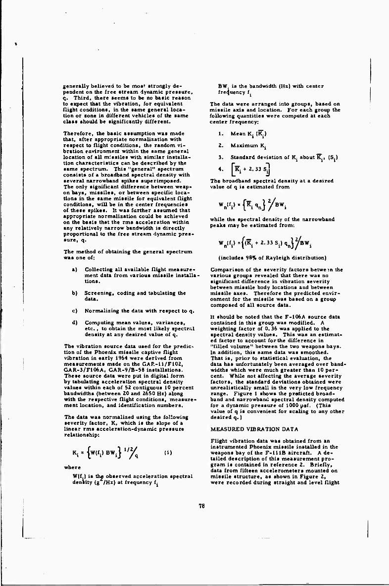
generally believed to be moat strongly dependent on the free stream dynamic pressure, q. Third, there seems to be no basic reason to expect that the vibration, for equivalent flight conditions, in the same general location or sone in different vehicles of the same class should be significantly different.

Therefore, the basic assumption was made that, after appropriate normalization with respect to flight conditions, the random vibration eavironment within the same general location of all missiles with similar installation characteristics can be described by the same spectrum. This "general" spectrum consists of a broadband spectral density with several narrowband spikes superimposed. The only significant difference between weapon bays, missiles, or between specific locations in the same missile for equivalent flight conditions, will be in the center frequencies of these spikes. It was further assumed that appropriate normalization could be achieved on the basis that the rms acceleration within any relatively narrow bandwidth is directly proportional to the free stream dynamic pressure, q.

The method of obtaining the general spectrum was one of:

a) Collecting all available flight measurement data from various missile installations.

b) Screening, coding and tabulating the data.

c) Normalizing the data with respect to q.

d) Computing mean values, variances, etc., to obtain the most likely spectral density at any desired value of q.

The vibration source data used for the prediction of the Phoenix missile captive flight vibration in early 1964 were derived from measurements made on the GAP.-l 1/F102, GAR-3/F106A, GAR-9/B-58 installations. These source data were put in digital form by tabulating acceleration spectral density values within each of 52 contiguous 10 percent bandwidths (between 20 and 2650 Hz) along with the respective flight conditions, measurement location, and identification numbers.

The data was normalized using the following severity factor, K, which is the slope of a linear rms acceleration-dynamic pressure relationship:

(1)

where

Ki={w(fi)BWi}iyq

ere

W(f.) is thf observed acceleration spectral density (g /Hz) at frequency f.

BW. is the bandwidth (Hz) with center frequency f.

The data were arranged into groups, based on missile axis and location. For each group the following quantities were computed at each center frequency:

1.

2.

3.

4.

Mean K. {K.J

Maximum K;

Standard deviation of K- about K., (S.)

[^ + 2. 33 S;

The broadband spectral density at a desired value of q is estimated from

wn<v=("i %] y**i while the spectral density of the narrowband peaks may be estimated from:

Wn(f.)={(K. + 2.33S.)qnJ*/BW.

(includes 98% of Rayleigh distribution)

Comparison of the severity factors between the various groups revealed that there was no significant difference in vibration severity between missile body locations and between missile axes. Therefore the predicted environment for the missile was based on a group composed of all source data.

It should be noted that the F-106A source data contained in this group was modified. A weighting factor of 0. 36 was applied to the spectral density values. This was an estimated factor to account for the difference in "filled volume" between the two weapons bays. In addition, this same data was smoothed. That is, prior to statistical evaluation, the data has unfortunately been averaged over bandwidths which were much greater than 10 percent. While not affecting the average severity factors, the standard deviations obtained were unrealistically small in the very low frequency range. Figure 1 shows the predicted broadband and narrowband spectral density computed for a dynamic pressure of 1000 psf. (This value of q is convenient for scaling to any other desired q.)

MEASURED VIBRATION DATA

Flight vibration data was obtained from an instrumented Phoenix missile installed in the weapons bay of the F-111B aircraft. A detailed description of this measurement program is contained in reference 2. Briefly, data from fifteen accelerometers mounted on missile structure, as shown in Figure 2, were recorded during straight and level flight

78

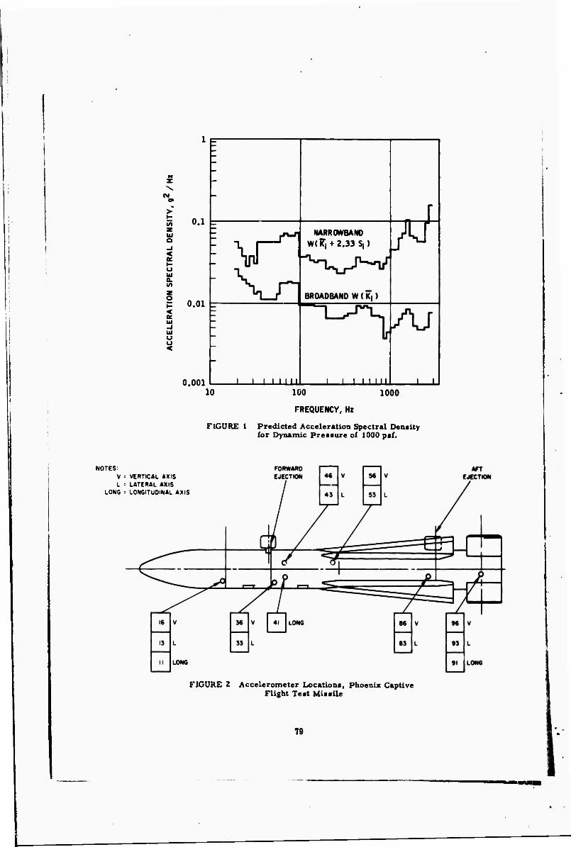
1 er

55

< t- u tu a.

0.1

I 0.01

o u <

0.001

!\n

J I I I I IM

NARROWBAND W( 7,-1-2.33 St) rf

J I I I I III J L 10 100

FREQUENCY, Hz

1000

FIGURE 1 Predicted Acceleration Spectral Density for Dynamic Preisure of 1000 p«f.

WOTES; V : VERTICAL AXIS L ' LATERAL AXIS

LONG : LONGITUDINAL AXIS

FIGURE 2 Accelerometer Locations, Phoenix Captive Flight Test Missile

79

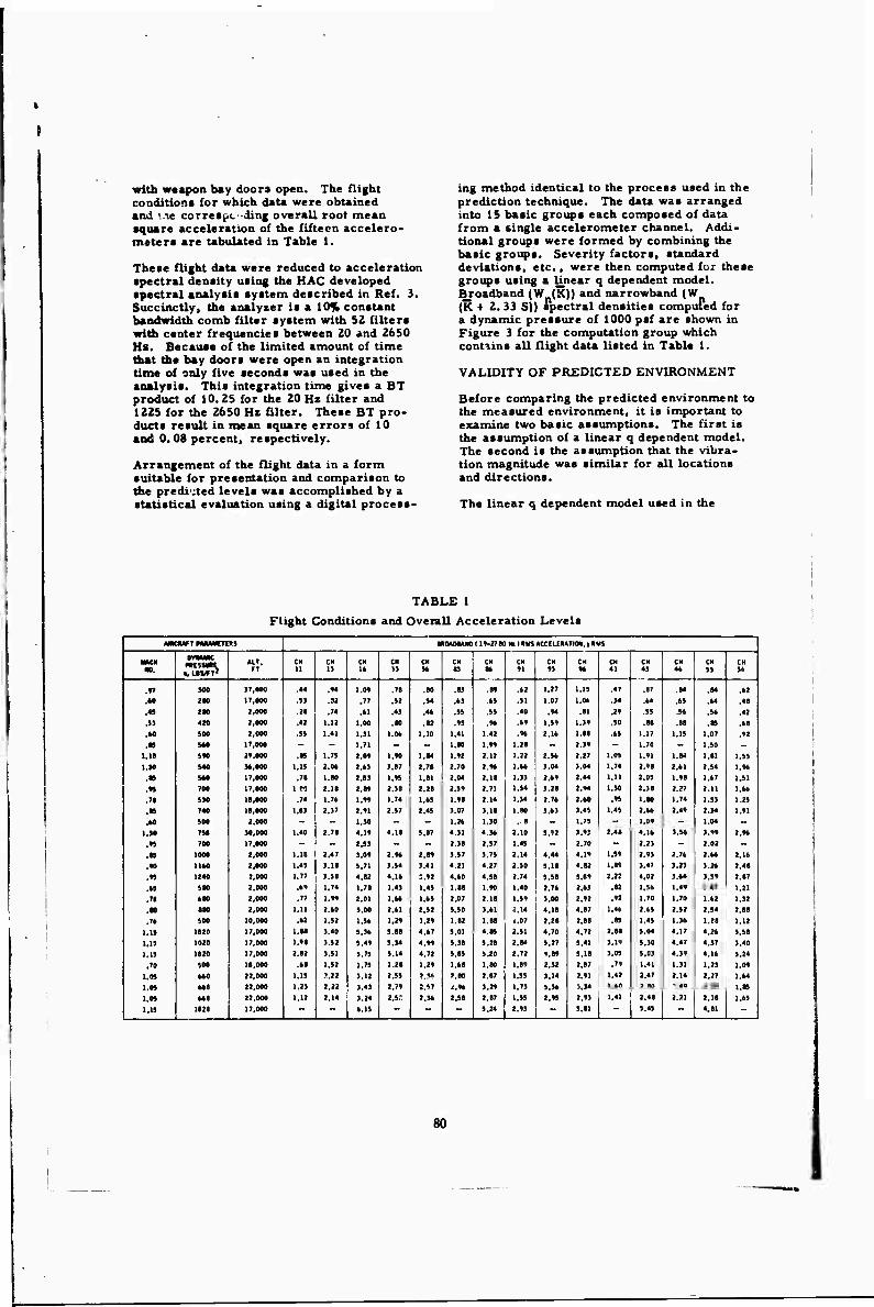
with weapon bay doors open. The flight condition« for which data were obtained and <.ie correa^C'ding overall root mean ■quare acceleration of the fifteen accelerometera are tabulated in Table 1.

Theae flight data were reduced to acceleration •pectral density using the KAC developed spectral analysis system described in Ref. 3. Succinctly, the analyser is a 10% constant bandwidth comb filter system with 52 filters with center frequencies between 20 and 2650 Ha. Because of the limited amount of time that the bay doors were open an integration time of only five seconds was uaed in the analysis. This integration time gives a BT product of 10. 25 for the 20 Hz filter and 1225 for the 2650 Hs filter. These BT pro- ducts result in mean square errors of 10 and 0,08 percent, respectively.

Arrangement of the flight data in a form suitable for presentation and comparison to the predicted levels was accomplished by a statistical evaluation using a digital process-

ing method identical to the process used in the prediction technique. The data was arranged into 15 basic groups each composed of data from a single accelerometer channel. Addi- tional groups were formed by combining the basic groups. Severity factors, standard deviations, etc., were then computed for these groups using a linear q dependent model. Broadband (W (K)) and narrowband (W (K + 2. 33 S)) spectral densities computed for a dynamic pressure of 1000 psf are shown in Figure 3 for the computation group which contains all flight data listed in Table 1.

VALIDITY OF PREDICTED ENVIRONMENT

Before comparing the predicted environment to the measured environment, it is important to examine two basic assumptions. The first is the assumption of a linear q dependent model. The second is the assumption that the vibration magnitude was similar for all locations and directions.

The linear q dependent model used in the

TABLE 1

Flight Conditions and Overall Acceleration Levels

MKUTT miuMrms «MOMW1 H-JT90 W 1 »US MCIUUTIM,, «MS {

MKII •0.

tmmc XKSSWC FT

CH 11

CD 13 1»

CH 13

CM 3*

CH 03

CH 8*

CH «1

CH 03

CH 0*

CH 41

CH 43

CH 4*

CH 93

CH 9*

.n 300 97.000 .44 .04 1.00 .70 .00 .83 .0» .42 1.27 1.19 .47 .87 .84 .H .»»

.M too 17,000 .33 .32 .77 .92 .94 .*3 .09 .91 1.07 1.0* .34 .64 .*5 .04 .40

M IM 2,000 .20 .74 .»1 .43 .44 .59 .93 .40 .0« .81 .20 .95 .9* .9* .42

.53 •M 2,000 .42 1.12 1.00 .W .82 .03 .0* .49 1.90 1.30 .90 .88 .M .89 .*8

.M 500 2,000 .95 1.41 1.31 l.Ot 1.10 1.41 1.42 .0* 2.16 l.M .69 1.17 1.13 1.07 .02

•■ 940 17,000 - - 1.71 l.M 1.00 1.28 - 2.30 - 1.70 - 1.90 - 1.10 500 2«,000 .09 1.79 2.0* 1.00 l.M 1.02 2.12 1.22 2.5* 2.27 1.09 1.01 l.M 1.01 1.11

I.J0 540 34,000 1.19 2.M 2.03 3.07 2.70 2.70 2.0* 1.** 3.04 3.04 1.74 2.00 I.« 2.94 1.0*

.a 5U 17,000 .71 l.M 2.03 1.05 1.01 2.04 2.18 1.33 2.6' 2.44 1.11 3.03 1.00 l.*7 1.11

.♦» »00 17,000 1.00 2.10 2.« 2.30 2.28 2.99 2.71 1.94 3.28 2.04 1.30 2.18 3.37 2.11 1.6*

.n 530 10,000 .74 1.7t i.r> 1.74 1.09 1.08 2.14 1.34 2.7* 2.60 .09 l.M 1.74 1.93 1.29

.m 740 10,000 1.03 2.37 2.01 2.97 2.45 3.07 3.10 l.M 3.*3 1.49 1.49 2.6* 3.40 3.14 1.01

M 500 2,000 - - 1.30 - - 1.2* 1.30 . B - 1.73 - 1.00 - 1.04 - l.M 790 30,000 1.40 2.78 4.10 4.10 3.87 4.31 4.3* 2.10 3.02 3.0J 2.48 4.16 3.9* 3.00 2.06

.» 700 17,000 - - 2.93 - 2.38 2.97 1.49 - 2.70 - 2.21 - 3.02 -

.B 100« 2,000 1.11 2.47 3.00 J.ot 2.80 3.97 3.79 2.14 4.44 4.10 1.50 2.03 3.76 2.0* 2.16

.«0 1100 2,000 1.43 3.10 3.71 3.94 3.41 4.21 4.27 2.90 9.18 4.82 1.00 3.47 3.23 3.2* 2.48

M 1240 2,000 1.77 3.91 4.02 4.10 3.02 4.*0 4.90 2.74 5.58 9.00 2.22 4.02 3.*4 3.90 2.87

M 500 2,000 .6» 1.74 1.71 1.43 1.45 l.M 1.00 1.40 2.76 2.63 .82 1.96 1.40 1.47 1.21 .n »00 2,000 .77 1.« 2.01 l.M 1.49 2.07 2.10 1.90 J.00 2.02 .02 1.70 1.70 1.62 1.12

.a> too 2,000 1.11 2.t0 3.00 2.01 2.92 3.90 3.61 2.14 4.10 4.07 1.4* 2.t9 3.93 2.94 2.08

.it 500 10,000 .»» 1.92 1.9t 1.20 1.20 1.82 l.M 1.07 2.20 2.08 .85 1.49 1.3* 1.28 1.12

1.15 1020 17,000 l.M 3.40 9.3* 5.00 4.67 5.01 4.89 2.91 4.70 4.72 2.88 5.04 4.17 4.2* 1.38

1.15 1020 17,000 l.M 3.52 9.40 9.34 4.00 9.30 9.20 2.M 5.27 5.41 3.10 9.30 4.4} 4.37 3.40

1.15 1020 17,000 2.02 3,91 9.79 9.14 4.72 9.03 9.20 2.72 1.80 9.18 3.05 9.03 4.30 4.1* 3.24

.»o 500 10,000 .ti 1.92 1.79 1.20 1.20 l.*8 l.M 1.00 2.32 2.07 .70 1.41 1.31 1.23 1.00

1.05 tu 22,000 1.13 3.22 3.12 2.99 ».}« 3.00 2.87 1.95 3.14 2.01 1.42 2.47 3.14 2.27 l.*4

1.05 tto 22,000 1.23 2.22 3.43 2.70 2.97 i.0* 3.20 1.73 3.3* 3.34 l.*0 2.M 3.40 2.18 1.09

1.05 too 22,000 1.12 2.14 3.24 2.5.- 2.3* 2.98 2.87 1.53 2.05 2.03 1.41 2.48 3.21 2.18 1.69

1.15 1020 17,000 - — t.19 - - 9.24 2.03 - 9.81 - 9.49 - 4.81 -

80

1 p:

CM

>

<

0.1

Q. V>

Z

p 0.01 < B UJ

o <

0.001 10

-»Ö

n |i 11 i, • i

i i i j

I H t, äe

Vn 1J;

rVV''

ii WÖf,+2.33SI)il ' i LIi

Wh • •

„1/

II, ■ i

r- !

i/n

n/W W«,)

U 1 I I I I I I II. I I Mill

JL

V i

J ',

i

1/ R1

1 100

FREQUENCY, Hz

1000

FIGURE 3 Mean and Extreme Acceleration Spectral Demitiea fo;r Dynamic Pressure of 1000 pef. Computed for Group coixposed of all Flight Dati

statistical evaluation of the flight data implies that the rms acceleration in any bandwidth (for a given accelerometer location) is directly proportional to the dynamic pressure. This assumption was based on observations of data from many previous flight measurements. It implies that the spectrum shape remains

1. Mean frequency (F) =

comitant (i. e., the npectrail density will increase everywhere by a dticade for a 3.16 factor increase in dynamic pressure).

During the computer evaluation of the Phoenix flight, data the following parameters were calculated for each spectrum:

52

y W{f.) x SW. x fj

i = t

I *<V xBW.

Area Moment radius about ?(iV. ) =

52

T WJfj) v. BW. x r2

-ife

i a 1 TT W S W(f.)xBW.

i = 1

81

3. Overall Severity Factor (K ) =grm»/q

At a given location, these parameters should be constant for all flight conditions if the data follows a linear q model. Table 2 liitr the values of thuse parameters with their corresponding flight coaditions for the data from accelerometer 33.

It is evident from this table that, for this particular channel, the spectrum shape and overall severity have a definite trend with Mach No. The mean frequency and overall severity factor increases with increasing Mach No. aid the radius of gyration about the mean frequency decreases with Mach No. The overall severity factor (KU» plotted vs Mach No. for this channel in Hgure 4. This figure is typical of all channels and indicates that the overall severity has an increasing trend with Mach No. The deviations from the linear q model in the frequency domain can be studied by examining the parameter S./IT, shown in Figure 5 for the data from accelerometer 36. The values shown on this curve are typical of all channels. It is apparent that there is more spread in the higher frequency region (i.e., the standard deviation over mean severity factor is significantly higher in the

a 0.0100

0.0075

^ 0.00S0

" 0.0025

a *LT>»K Ä MK>ALT >1SK

O I0K>ALT>5K

O 5t(>ALT A a

oioo^ £

"1 0.2 O.f. 0.8

MACH NUMBER

1.0 1.2 1.4

FIGURE 4 Overall Severity Factor Versus Mach No. - Accelerometer No. 33

TABLE 2 Spectrum Characteristics Channel 33

Dynamic Altitude Pressure F R

Mach No. Ft psf Hz HS Ko

0.45 2000 280 924 738 0.00152 0.53 2000 420 1080 670 0.00190 0.60 2000 500 1087 674 0.00213 0.60 17000 280 939 697 0.00186 0.65 2000 580 1149 653 0. 00246 0.70 10000 500 1175 659 0. 00256

[ 0.70 2000 680 1189 638 0. 00245 0.70 10000 530 1232 606 0. 00328 0.76 10000 500 1072 655 0. 00257 0.80 2000 880 1225 610 0. 00297 0.85 2000 1000 1294 567 0. 00296 0.85 10000 740 1282 569 0. 00348 0.85 17000 560 1270 569 0. 00348 0.90 2000 1160 1305 565 0. 00305 0.95 2000 1240 1330 549 0. 00336 0.95 17000 700 1302 558 0.00339 0.9 37000 300 1177 633 0. 00260 1.05 22000 660 1321 555 0. 00382

1 1.05 22000 660 1334 533 0. 00422 1.05 22000 660 1350 534 0. 00387 1.15 17000 1020 1395 478 0. 00504

1 1.15 17000 1020 1395 470 0. 00524 1.15 17000 1020 1396 473 0. 00498 1.30 30000 750 1423 462 0. 00558 1.30 36000 540 1401 471 0. 00569

82

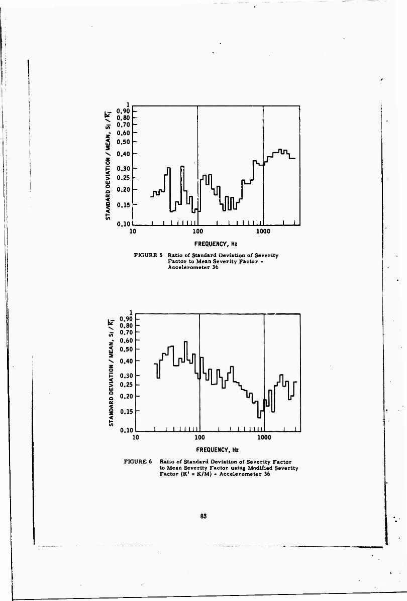
2 2

< > Li a a at

2 z <

0.90 - 0.80 - 0.70 0.60 0.50 -

0.40 -

0.30 0.25 h

0.20

0.15

0.10 10

ji n

J^

Lr v W J ' i i I in J J L

100

FREQUENCY, Hz

1000

FIGURE 5 Ratio of Standard Deviation of Severity Factor to Mean Severity Factor - Accelerometer 36

FREQUENCY, Hz

FIGURE 6 Ratio of Standard Deviation of Severity Factor to Mean Severity Factor uting Modified Severity Factor (K1 ■ K/M) - Accelerometer 36

83

upper frequency range). In effect this means that either the model is less satisfactory in the high frequency region or that there «re more perturbations (*.e. , non-linear effects, etc.) at higher frequencies. From the previous discussion of the data in Table 2. it was noted that the mean frequency of the spectrum increased with increasing Mach No. All this strongly suggests that the high frequency vibration severity is a function of both Mach No. and the dynamic pressure, while the low frequency range is mostly dependent on dynamic pressure alone. To further examire this trend, the data were re-evaluated using the following model for severity factor:

,• 0.0100

g 0.0075

> 0.0050 —

0.0025

oo^oS^SocPloo0

0.2 0.4 0.6 0.8

MACH NUUBH

1.0 1.2

<-h-«,}"/, qxM

FIGURE 7 Overall Severity Factor (20 - 400 Hz) vs Mach No. Accelerometer 36

Figure 6 contains a plot of S./K. for the data from accelerometer channel 36. This can be compared to the plot in Figure 5 which is a plot of the same quantities calculated for the linear q dependent model. This comparison shows that the ratio of S./K. is greatly affec- ted by the model chosen. In the low frequency region below approximately 400 Hz the linear q dependent model has the lowest ratio of S./K.. Above approximately 400 Hz the q x M model has the lowest ratio of S./E.. A final examination of this trend was performed by computing the overall acceleration level below 400 Hz for the data from accelerometer channel 36 using a linear q dependent model. The overall severity factor (K ) based on the recomputed acceleration levels is plotted vs Mach No. in Figure 7. Nöte that the trend with Mach No. is insignificant thus indicating a linear q dependent model is valid for this frequency range. In conclusion, the linear q dependent model is satisfactory except in the high frequency (above 400 Hz) range of the spectrum where the severity factor increases with increasing Mach No. At present there has been no investigation of tt: causes of this Mach No. dependency, which, if present, was not evident in other installations. For the purpose of comparing the measured and predicted environments, the linear q-dependent model is satisfactory since:- 1) the prediction employed a linear model; 2) the model is very accurate for 4 1/2 octaves of the 7 octave bandwidth; 3) the Mach No. effect changes the levels significantly only for high q and high Mach No. conditions for which no data exi«ts; and 4) the difference in standard deviations of severity factors above 400 Hz for the two models (see Figures 5 and 6) is not overwhelming.

During the prediction study, the missile vibration data was evaluated for groups of data from various regions of the missile (i. e., mid, aft, forward and missile axes). However, because no significant differences between regions were found, the Phoenix requirements were based on an evaluation group composed

of all locations and directions. The flight data was examined for these trends by comparing mean severity factors between various regions and directions. After comparing the various severity factors it was concluded that with the exception of the lateral aft region, which was slightly more severe than any other location, vertical and lateral vibration severity was similar throughout the missile. Longi- tudinal severity factors were approximately one half the severity factors for the vertical and lateral directions.

A comparison of the predicted environment to the measured environment on an overall or volumetric basis can be made by examining Figures 8 and 9. Figure 8 is a plot of the ratio of mean severity factors vs frequency and Figure 9 is a plot of the ratio of the ratios of standard deviation to mean severity factor vs frequency.

Figure 8, the ratio of mean severity factors, indicates that the predicted severity factor compares very closely with the measured severity factor. The ratio oscillaves about a value slightly less than unity. Only two frequencies exceed + 3 db which is unconservative while three clusters of three or four frequencies exceed - 3 db, approaching - 6 db. Considering the customary ± 3 db tolerance used in vibration testing, the difference between predicted and measured values is considered small. The ratio of the ratios of S/K indicates that there is more spread in the measured data (i.e., this ratio oscillates about a value greater than unity).

In the very low frequency (below 35 Hz) only the previously smoothed data contributed to the predicted values. Thus unrealistically low S./Kj (predicted) values influence Figure 9. Above 250 Hz, the previously discussed Mach

84

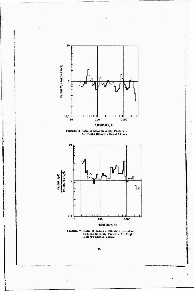
100

FREQUENCY, Hi

FIGURE 8 Ratio oi Mean Severity Factor» - All Flight Data/Predicted Value»

10

vT a u O 5 UJ K 0.

0.1

ml

JA^ÜC Rrij

i i mil i ! i i mil i i

^ t

10 100

FREQUENCY, Hi

1000

FIGURE 9 Ratio of Ratio» oi SUndard Deviation to Mean Severity Factor - All Flight OaU/Predicted Value»

85

N3. effect tends to give high S./fT values. Even allowing for these factors, u does appear that the variability of severity factor within a missile is as great as the variability between different missile/aircraft installations.

LABORATORY VIBRATION SIMULATION

It is customary to describe the laboratory vibration environment in terms of the specified vibration excitation of a test item. In this case, the degree of laboratory simulation would be assessed in terms of simulation of excitation. However, to be consistent with the prediction technique employed to derive the vibration test parttmeters, both excitation and response vibration levels are controlled, as described in Ref. 3. Then both excitation and response levels may enter into assess- ment of the simulation. However, for the missile test, no attempt was made to simulate the excitation in the testir.« .i *he missile. During captive flight with bay due rs open, the excitation is aerodynamic and occurs over the entire missile surface whereas in the laboratory the excitation is applied to the missile at a single point for any one test. There is, therefore, no simulation of modal excitation. It should be expected that the dynamic rela- tionships between locations in the missile that occur in captive flight will not be dupli- cated in the laboratory.

Therefore, in the laboratory test, no attempt was made to duplicate the vibration level at particular missile locations. Rather the objective of the method was to produce an "average" or "volumetric" vibration response throughout the missile equivalent in severity to the predicted response. It will be seen that the use of multiple successive excitation points to achieve this objective is crucial. The following method was used in an attempt to simulate this average response.

The missile, suspended by the launcher attachments, was subjected to broadband random vibration. The excitation was successively applied at the forward and aft ejection bulkheads for the vertical and lateral directions and, since it was the only practical location, at the aft end of the missile for the longitudinal direction.

Accelerometers at the excitation locations were controlled to a spectral density based on the predicted mean value (W (K)) shown in Figure t. Other accelerometers were locate I at a number of locations on missile structure representative of likely locations for flight measurements. The spectral density values at these accelerometers wnre limited to a value based on the extreme spectral density (W (7 + 2. 33S)) of Figure 1 by reduction of the excitation in narrow frequency bands which corresponded to frequency bands of maximum response. A detailed description

of the implementation of this test method is included in Ref. 3 and will not be repeated here.

To compare the results of the laboratory tests to the measured environment, il was necessary to treat the test data as if it were a set of flight data, all measured at a dynamic pressure equal to the dynamic pressure upon which the test levels were based. For each accelerometer location, a maximum vibration spectrum wa» computed by enveloping all spectra obtained at that location during the several excitations. These maximiun spectra v/ere then normalized with respect to q and equivalent severity factors computed. These data were then formed into comparison groups analogous to those used in evaluating the flight data. Mean values and standard deviations of the severity factor for these groups were computed.

It would perhaps be most natural to compare the test results to the predicted environment in order to assess the degree of simulation achieved. However, the measured environment was now at hand and the major emphasis was to assess the degree to which the test had simulated the measured environment. Since, as discussed earlier, the measured and predicted environments were in good agreement, comparison to the measured environment was satisfactory.

Figures 10 and 11 demonstrate the degree to which the "volumetric" missile response was simulated. Figure 10 is a plot, vs frequency, of the ratio of the mean severity factor from flight data to that from laboratory test with all data included in the groups, similar to Figure 8, Figure 11 is a plot, vs frequency, of the ratio of the ratios of standard deviation to mean severity factor, similar to Figure 9, Close simulation is achieved if these two plots are close to unity across the frequency range although it is probably desirable to have the K ratios somewhat less than unity to achieve some conservatism. From Figure 10, it is concluded that the test levels were somewhat deficient above 200 Hz while from Figure 11, it appears that the maximum response spectral density was set at too low a level (relative to the maximum input spectral density) since the S/K ratio oscillates about a value greater than unity. However, during the laboratory tests there were only a few frequency bands where excitation was reduced in order to limit the response and these were usually below 200 Hz. Thus it is believed that the major factor in the inadequacy of the test levels above 200 Hz was in fact due to the rapid attenuation with distance from the excitation point. In the higher frequency region, there was very little amplification of the excitation and the extreme response values were not approached. This factor points out the difficulty of simulating aerodynamic

86

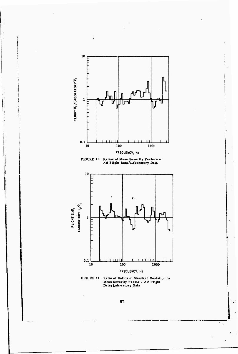
100

FREQUENCY, Hz

1000

FIGURE 10 Ratio« of Mean Severity Factor» All Flight Data/Laboratory Data

»- z o

> g < B CO

3

i i i mil i i i i um i i 100 1000

FREQUENCY, Hz

FIGURE 11 Ratio of Ratios of Standard Deviation to Mean Severity Factor - AH Flight Data/Laboratory Data

87

excitation by «ingle point excitation and the need to conduct aaccessive excitation at a number of points.

la «pite of these difference*, it 1* believed that Figure* 10 and 11 «how that the degree of laboratory •imulation, judged on the baai* of all acctlerometer location*, wa* remark- ably good.

The degree of •imulation achieved at a particular location it, a* should be expected, less satisfactory and highly variable. Figures 12 and 13 present the ratio of K from flight data to test data for the forward ejection bulkhead in the lateral and vertical directions respectively. These were excitation point* during te*t. In this case, R for the teat data is actually the severity factor from the maximum test spectrum for that location. Since the ratio of the maximum to the mean severity factor for the flight data was between 2 and 3, good simulation would be achieved if the R ratio* in these figures fluctuated between unity and approximately 0. 3. Figures 14 and 15 are similar plots for the guidance unit bulkhead in the lateral and vertical directions respectively, which were reaponae control locations during teat. The difficulties of simulating an environment in any detail at a number of points i* readily apparent from the variation* in and between the*« four figure*.

In addition to the previously mentioned difficulty due to attenuation with distance from the excitation, it i* now apparent that u*e of a eingle accelerometer for input level control al*o contributed to the degraded simulation. A* di*cu**ed in Ref. 3, u*e of a single accelerometer prevents the occurrence of a spectral density value greater than the msan value, at least while excitation i* applied at that point. To explore the possible improvement in simulation to be achieved by uae of the power average of aeveral accelerometer signals for the teat level control, the laboratory teat data for vertical excitation at the forward ejection bulkhead waa examined. Figure 16 ia a plot rf the apectral denaity at the input point and the maximum reaponae spectra! denaity ob- aervsd at any other location on the miasile uaing the aingle accelerometer for input level control. Figure 17 is a plot of a computed input apectral denaity, uaing the power average of three accelerometer signals and the computed maximum response spectral density which would occur with the computed input, assuming linearity of response. A detailed discussion of the locations, etc, of these maximum response spectra is beyond the scope of Ulis paper. However, the improvement in simulation of the high frequency spectrum above 200 He is evident from comparison of these figures.

CONCLUSION

This paper has attemped to describe, within reasonable limitations of time and space, the results ol :fforts spanning almost five years covering the prediction, the simulation, and finally, the measurement of the captive flight vibration environment of the Phoenix missile. While the title selected (before much of it was written) was perhaps rather strongly worded, the study is believed to illustrate the basic validity of the prediction and test methods described while pointing out some of the limitations which generally face the dynamicist working on this type of problem.

The major conclusions which the authors draw are as follows:

1. O.i an overall or "volumetric" basis, the prediction technique yielded very satisfactory results.

2. On a similar basis, the simulation technique also yielded satisfactory results.

3. Neither the prediction technique nor the simulation technique should be expected to match the measured environment in much detail. Further the variability observed in the measured environment was such that the likelihood of any technique being able to do so appears quite small.

4. Although it has been rather generally agreed that the linear q^dependent model is a valid one, the discovery of the Mach No. dependence for frequencies in excess of about 400 Hz for this installation was surprising and perhaps significant for future development of prediction techniques.

5. While the test methods employed en- tail some complexity, the vibration of test objects of significant dimensions and weight, such as the Phoenix missile can only have real significance with respect to the usage environment if: 1) the response of the test object is employed in control of the tests; 2) the excitation is applied at a number of points, either successively or possibly simultaneously; and 3) the excitation is controlled from the power average of several accelerometer*.

88

100

FREQUENCY, Hz

FIGURE 12 Ratio of Mean Severity Factors - Flight Data/Laborat jry Data, Forward Ejection Bulkhead Lateral

100

FREQUENCY, Hz

1000

FIGURE 13 Ratio of Mean Severity Factor« • Flight Oata/Labcratory Data, Forward Ejection Bulkhead Vertical

89

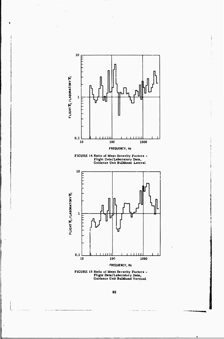
> g < s CD

100

FREQUENCY, Hi

1000

FIGURE 14 Ratio of Mean Severity Factors - Flight Data/Laboratory Data, Guidance Unit Bulkhead Lateral

>

< g as 3

100

FREQUENCY, Hz

1000

FIGURE 15 Ratio of Mean Severity Factor« • Flight Dau/Laboratory Data, Guidance Unit Bulkhead Vertical

90

1 F

0.1 r UJ a

<

K 0.01 <

IU u <J

0.001

MAXIMUM RESPONSF ENVELOPE

J ̂

3 INPUT (SINGLE ACCELEROMETER)

I I II Mil

I IT

I! S

fc

"i

_IiL.

^

JL. I 11 llii J I 10 100

FREGUENCV, Mt

1000

FIGURE 16 Phoenix Missile Assembly Test - Envelope of Maximum Response Acceleration Spectral Density and Input Acceleration Spectral Density when Input is controlled from a single accelerometer.

1 F

0.001

FREQUENCY, Hi

FIGURE 17 Simulated Phoenix Missile Assembly Ttit - Envelop« of Maximum Response Acceleration Spectral Density and Input Acceleration Spectral Density if control had been power-averaged from several accelerometer s.

91

REFERENCES

2.

A. J. Curtit, "A SUtittical Approach to Prediction of the Aircraft Flight Vibration Environment", Shock and Vibration Bulletin 33 (Part I): 1-13, (19*4)

T. M. Kiwoir, R. P. Mandich and R. J. Oedy, "PHOENIX Environ- mental Meaeureniests is F=111S

Weapon« Bay", Shock and Vibration Bulletin 39. (To be published)

A. J. Curtis and J. G. Hererra, "Random Vibration Test Level Control Using Input and Test Item Response Spectra", Shock and Vibration Bulletin 37 (Part 3): 47-60. (1968)

DISCUSSION

Mr. jfcytor (Dgfaocg Research Establlsh- m«nt, Suffuikl. Canada): I do not remember yow otlglnal formula very closely, but I believe the severity was proportional to the dy- mmlc pressure. So it is proportional to Mach number squared. Now you find that this only applied up to 400 Hz. Above this it is propor- tinuil to Mach number cubed. I would like to fget your views on why this should be. I think maybe it is because vp to 400 Hz we have bending effects and beam vibratione in the missile, fcßd above this it goes Into panel resonances, aixl the panel resonances are more susceptible

to acoustic excitation. Would this theory have your support?

Mr. Curtis: I really think that the most honest was at answering that question is that we have not really tried to explain this phenomenon that we have found. It seems to be there, we have not had a chance to try to get an explanation. But it does seem to be something that should be Incorporated in future efforts in trying to make a prediction. I certainly have no quarrel with the postulate that you just made, but I am not sure that I am qualified to agree with it, either.

92

PHOENIX ENVIRONMENTAL MEASUREMENTS IN F-KIB WEAPONS BAY

T. M. Kiwior Mechaiiici Research, Inc.

El Segundo, California

R. P. Mandich and R. J. Oedy Hughes Aircr7.it Company, Missile Systems Division

Canoga Park, California

A description of the PHOENIX T-20 Data Acquisition liistnsmentation System is given. The PHOENIX T-20/r-IllB Bay Emiromnental Measurements Flight Test Program is discussed. Early unsteady bay pressure predictions and actual measurements are compared and discussed.

INTRODUCTION

A series of experimental captive flight environmental measurement tests of a PHOENIX missile in the weapons bay of an F-11 IB aircraft was conducted to measure and record vibration, shock, structural response, gross loads, temperature, aerodynamic pressure and acoustic environments. The measurement system consisted of two parts: A tactical missile with seunors and required signal conditioners, multiplex system, onboard tape recorder, and power regulation system substituted for various internal components; and a tactical launcher with flexure devices replacing the launcher ejector mechanisms to measure hook loads and missile gross loads. A total of eighty-six channels of data including aircraft parameters were recorded.

The first portion of the paper describes the flight test program, the hardware and instrumentation, and the performance of the measuring system in field usage. The second portion of the paper describes the fluctuating pressure measurements, the approach used to make early estimater of the severity of the bay unsteady pressures, and the comparison between estimated and measured values.

Captive flight environmental measurement tests of a PHOENIX missile in the weapons bay of an F-IlIB aircraft were conducted during the period of 30 March to 3 August 1967 to obtain data to verify and/or update the missile load and environmental design requirements. The instrumented missile system consisted of an instrumented missile, instrumented launcher, and a magnetic tape recorder carried within the missile. The program was limited to environmental measurements in the weapons bay without any adjacent stores.

The original captive flight vibration and acoustic pressure environmental design

requirements for the PHOENIX missile were determined by grouping, sculing, and extrapo- lating measured data from various air-to-air missiles flown on other aircraft. The missile and launcher dynamic loads were p> «dieted from th« estimation* at the bay pressure excitations. The confidence intervals associated with the vibration, fluctuating preoiiars, and dynamic load predictions «ere such tbut experimental verification of the design levels was required.

PHOENIX T-20 MISSILE

The PHOENIX T-20 meaattremeiot system was dependent on the mother aircraft lor powor and recorder command signals only. This wa» desired to minimise changes to the aircraft to accommodate the missile, and was pnrtieularly advantageous since measurements were to be obtained on the wing pylon as well as in th« bay.

The missile employed in obtaining th« tts- vironmental measurement« in this test program was designated T-20. In order to provide meaningful measurements of actual conditions, T-20 was designed to be dynamically similar to the tactical missile. It utilised a tactical fuselage, tactical wings and control sarfaces, tactical radome, and a tactical (inert) rocket motor. The data acquisition instrumentation was substituted for various internal components, but tactical weight and center of gravity were maintained. Temperature measurement» inth« bay were made primarily to evaluate temperature effects on the dynamic instrumentation.

The missile instrumentation system consisted of sensors and required signal conditioners, a multiplex system, tn onboard tape recorder, a power regulation system, and associated electrical wiring. Special fore« measuring mechanisms were designed, fabricated, and installed in the bay launcher to mat«

93

the Uuncher to the PHOENIX miiaile. A description of the meaeurement syatem, transducer«, channel frequency reaponaea. locationa on the T -20 miaaile, and multiplex frequency band are preaented in the following text. A block diagram of aenaor locations ia ahown in Figure 1.

The miaaile wa» inatrumented with 19 cryatal accelerometera having a frequency reaponae range from 5 to 2000 Hs, and 4 atrain gage accelerometera with a frequency range from 0 to 300 Ha. The tranaducera were mounted at various miaaile stations along the longitudinal, lateral and vertical axes.

All accelerometera located in the miaaile fuselage were calibrated to ±25g pk-pk. Fig- ure 2 ahowa a front view of the guidance aection bulkhead with two strain gage accelerometera &nd ampllfiera and three cryatal accelerometera Inatalled. The large ateel cylinder in Figure 2 is ballaat to maintain c. g. and weight require- menta. Figure 3 ahowa the accelerometer installation at atation 59.5 between the armament and guidance aections. The accelerometera at stations 127 and 146 are shown in Figures 4 and 5. respectively. Figure 6 ahowa the accelerometera at Station 82.3 aa well aa a number of aignal conditioning amp'ilflera.

Acouatic Microphonea

Two cryatal microphonea were mounted flush with the missile fuselage, one at missile station 39 at 6 o'clock and another midway between control surfaces 3 and 4 at 9 o'clock (looking forward). The microphone-amplifier systems were calibrated to measure a maximum of 162 db within a frequency band from 10 to 10,000 H*. The microphones were later re- calibrated to 173 db full scale to avoid clipping occasional peaks anticipated at the more severe environments.

Resistance Thermometers

Temperature sensitive film resistors of a nickel base material were used to detect temperatures. These were electrically connected in a one active arm bridge to produce a full scale signal variation for temperatures from -7»Of to +300oF. A typical installation is shown in Figure 7.

Pressure Transducers

Nine strain gage pressure transducers •sith dc amplifiers were installed on the missile. These were located on the right side, left side, and bottom cf the missile near the front, middle, and aft sections of the missile. The transducers employed were the absolute pressure type, calibrated to 25 psia to allow for the altitude effect on pressure. These «•nsors were capable of measuring quasi- static pressure variations.

Force Measurement Mechanisms

Th« ejection hook boxes, mounted in the launcher to which tho missile hooks normally attach, were replaced with specially designed Force Measurement Mechanisms (FMM). These units were designed specifically for the F-111B bay launcher and pylon. Figure 8 shows a sketch of an assembled FMM while Figure 9 shows an exploded view. Two of these units were required to mate the missile and launcher, one for the forward hooks and one for the aft hooks. A third unit was fabricated and maintained as a spare. The FMM had strain gaged load links arranged to measure 4 forces, right and left vertical, lateral and longitudinal.

Since the PHOENIX aft hooks are designed to transmit no longitudinal load, the aft longitudinal link was not monitored. Thus, seven data signals defined the three missile loads (vertical, lateral, longitudinal) and three moments (roll, pitch, and yaw).

Individual tests were performed on the force measurement mechanisms to calibrate them for measuring missile hook loads. The calibration loads were applied using a special loading fixture both along one axis at a time, and with six load components applied simultaneously. A statistical twenty-five point combined loading schedule was utilised for the combined loadings. Calibration constants were determined using a multiple nonlinear regres - slon digital computer program. The coefficients were subsequently utilised to determine missile hook load« from flight test signals.

Two force measurement mechanisms were then Installed in the bay launcher and a combined missile-launcher test performed to calibrate the launcher for missile gross loads and moments. The test consisted of installing the missile on the launcher in a loading fixture, applying combined loads and moments, and measuring the resultant FMM signals. Distrib- uted loads were applied by means of mechanical Jacks and whiffle trees. A similar statistical twenty-five point combined loading schedule and the multiple nonlinear regression digital computer program were used to determine calibration constants. The coefficients from this test were utilised to determine missile gross loads and momenis from the flight measurements.

Wing and Control Surface Bending Transducers

Forward and aft wing lugs as well as control surface shafts were Instrumented with strain gages to sense bending moments. Con- trol surface shafts were also instrumented to sense torsion. Typical wing lug and control surface strain gage Installations are shown in Figures 1C and 11. respectively. All of the strain gaged missile components produced approximately ±10 mv full-scale signal for full- scale load. These data channels employed low Input level voltage controlled oscillators (VCO)

94

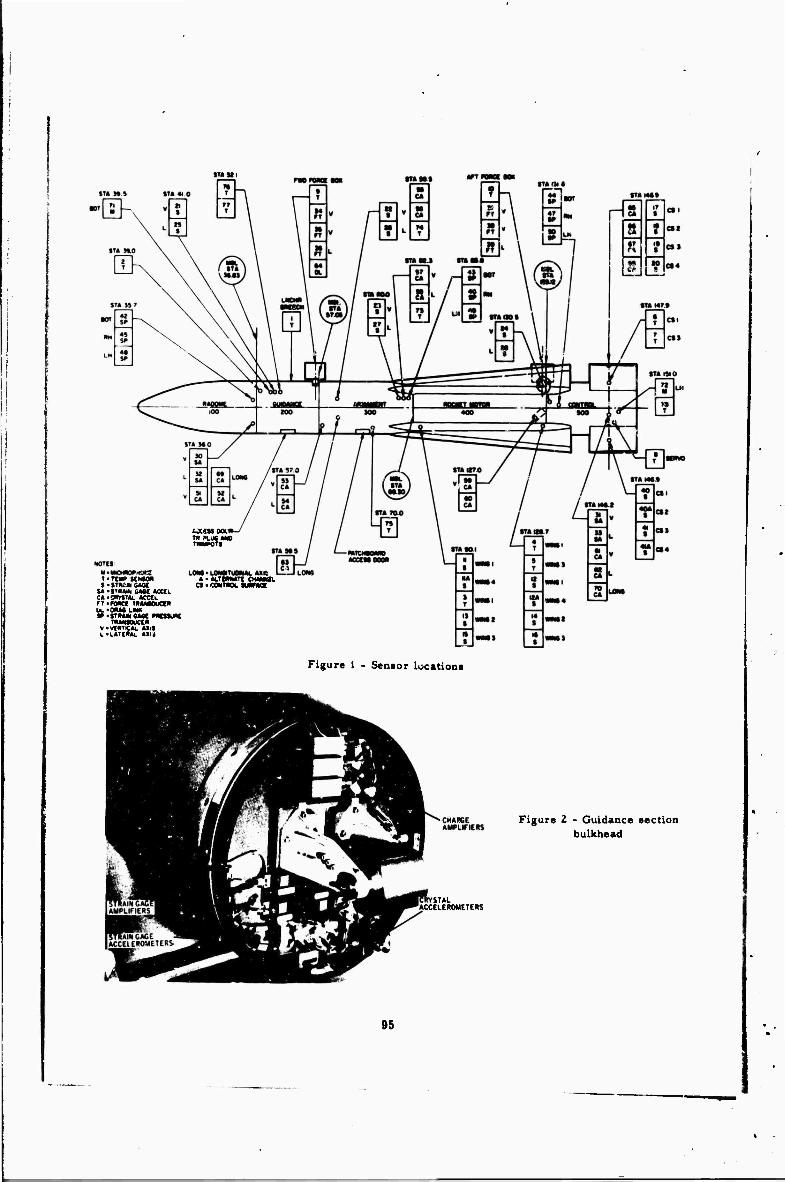
T • TCI» WMO* S • STKi« OMC

M •truM use «at i. »•conru. «cciL n-reoct TUMWUCII) U-'OMS LMI j» •tt*««OMC ncuuoc

nuimucc* V < VdlTICU. «Ill i. •L*Tt««L «Hi

WC!HOOl) T« MX MB Trnvort

LOM• LOMITUOM««. ... « • «LTtRWTt CHtMIIL

ct • ixmncn. *mna

Figure 1 - Senior location*

Figure 2 - Guidance section bulkhead

ST»L ACCELEROMETERS

95

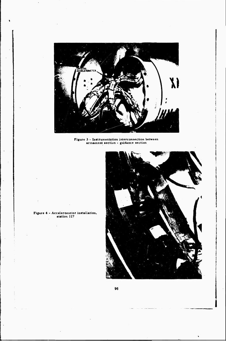
^Kä - J

K f

ACCCLEROMETER. ^ PB IP^" \

i Figure 3 - Inatrumentetion interconnection between

armament section - guidance section

Figure 4 - Accelerometer installation, station 127

96

Figure 5 - Accelerometer inrt .lUtion, station 146

Figure 6 - Aft view of armament section

97

.

Figure 7 - Typical resistance thermometer installation

MSSILE HOOK RECCPTACI.ES

LATER«. LOAD SCflM*

VERTICAL LOAD SENSORS

Figure 8. Assembled view, force measurement mechanism

Figure 9 - Exploded view, force measurement mechanism

98

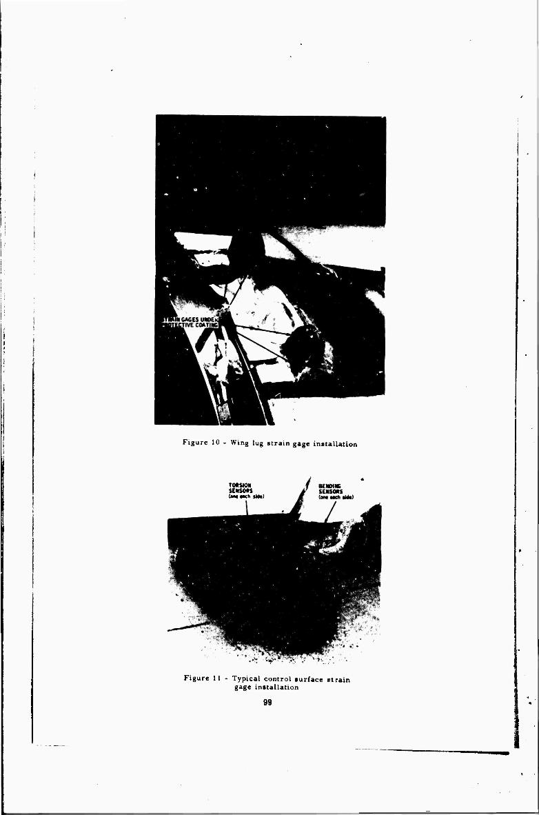
Figure 10 - Wing lug strain gage installation

TMSKW SENSORS (ant MCh iWcJ

BCNOINC SENSORS

Figure 11 - Typical control surface strain gage installation

99

in the multiplexer tection of the data acquieition ■yatetn.

Both the wing lug and control surface strain gage transducers were load calibrated. Full- scale load was first applied, and the signal conditioning circuit adjusted for full-scale output. Loads were then applied in increments of 20% of full scale, and the output voltages recorded. A standardisation resistor was shunted acroas one leg of the bridge, and the resulting output was also recorded. The minimum least squares linear fit was determined for each tranrducer.

Fnaelage B»g.*ing and Launcher Attach Link Strain Sages

Strain gage transducers were installed on the T-20 fuselage to measure bending. Verti- cal and lateral sensors were installed at stations 41, 59.5, and 80.

The launcher as mounted in the bay of the F-111B is attached by redundant brackets on the outboard side and pinned by links on the inboard side. These inboard links were equipped with strain gages and calibrated to measure the loads transmitted from the launcher to the bay floor.

MULTIPLEX/DEMULTIPLEX SYSTEMS

Multiplex System

The multiplex system consisted of 84 subcarrier voltage controlled oscillators (VCO), one reference oscillator, 13 mixer amplifiers, one VCO voltage calibrator and a mounting chassis with the necessary interconnecting wiring, connectors, and test points. The multiplex system provided a means of recording 84 channels of data on 12 tracks of a 14-track onboard tape recorder. Each of 12 mixer amplifiers accepted the outputs of seven subcarrier oscillators. The seven subcarrier frequency bands were the same for each of the 12 tracks. The subcarrier voltage controlled oscillators changed the analog data being measured into frequency modulated data. The amplitude of the analog signal became the magnitude of the oscillator frequency, and the frequency of the analog signal became the rate of change of the oscillatcr frequency. This system at data recording had several advantages. It allowed simultaneous recordings of seven non- overlapping data channels on each tape track and it afforded greater accuracy than direct or analog recording. In addition, frequency modu- lation permitted recording dc signals which is not possible with direct recording. Data channels with c«nter frequencies of 5.4 kc, 12.5 kc, 20.8 kc, 29.2 kc, 37.5 kc, 64.0 kc and 96.0 kc were employed on each tape track. Figure 12 shows a schematic diagram of a typical track of data made up of seven channels. High level VCO's requiring an input signal of 0-5 volts were used for the amplified channels while low

level VCO's requiring 110 mv input signal were used with the strain gage channels. A 128 kc reference oscillator signal was mixed on each . -ack in order to provide a means of flutter compensation upon playback. An additional mixer amplifier was used at the output of the reference oscillator to ensure adequate isolation between multiplex tracks. A voltage calibrator provided precise calibration voltages simultaneously to all subcarrier oscillators. The calibrator also provided a calibrate command signal to operate the calibrate relays in each of the subcarrier oscillators.

Figures 13 and 14 show the bottom and top view of the Multiplex System/Tape Recorder Assembly on which the majority of the VCO's were mounted. Upon command from either the Ground Checkout Box, or the Aircraft T-20 Control Panel, the input to the VCO's was switched from the sensor signal conditioners to the calibrate relay. A three-level VCO calibration voltage was then sequentially fed to each VCO. In actual system operation, these calibration voltages were automatically recorded on the magnetic tape prior to each data run. The calibration sequence could also be msr.ually stepped from the Ground Checkout Box.

Demultiplex System

The demultiplex system (ground station} was used to convert the frequency modulated (FM) data, which was recorded in the direct mode on the missile tape recorder, back to a usable analog format. It consisted of 4 data discriminators, one reference discriminator, 2 delay lines, 13 channel selectors (filters), 10 output filters, one reference discrimination filter and one reference channel selector. This equipment enabled data to be reduced from any 4 channels on any two track* of either the even or the odd recorder heads. Tape speed compensation, using the 128 kc reference signal, was an integral part of this system. This tape speed compensation reduced the effect of tape recorder wow and flutter by 30 db.

TAPE RECORDER

The tape recorder and associated record electronics, as shown in Figure 14, was employed. Tracks 4 and 6 were standard FM to give a frequency response of 0-10 kc desired for acoustic data. The remaining 12 tracks employed direct record electronics with a frequency response of 500 cycles to 150 kc. The tape transport system had a capacity of 1200 feet of one inch wide, one mil tape. The machine operated at 30 inches per second providing a total available recording time of 8 minutes. The recorder head configuration was standard IRIG allowing tape playback on any other IRIG tape machine. Although the data on all tracks was frequency modulated, it was recorded in the direct mode, and therefore had to be played back with direct reproduce amplifiers through the demultiplex system.

100

:mmn mmmtk tmtf* nmmA : sikrA tr«rn I *a0tt MM sera/ sen/

»•tn.

FMO MS»

CHMMC

I t t, vco

M.OKC ±««c

ML

FMO

0/900 CM

COM

tit vco

MOHC ±0KC

HL

i-i

FFMO MSF O/WO

CM

r1 SKNM. JM»L

^

vco srsHc ttKC

HL

FMB »tW \ 0/900 CM I

MLMCX «LCVCL MMUST

l_i vco

MJWC ttw

HL

I HI)

FMO MSP

OC

ftUVCI. •AJUST

S 1

i t t VCO

fOMCC ttKC

i-i

AlRCHAFT SlSNAL CONOITIOMM

ST.« « CBSITATICH

MC Ml PW« ALL «»— OTHC* UMTS

MS (OVDC

MS CSVOC

SWNM. eons

vco its« ttw

LA

«£« Ml rm* TO TEMP SCMOM

, I MS I

C*L

-S*l_ VOLTMC lOUWCt —I—

CM.«

C»U« OMMAI

VCO S.4KC

HI

t t t t t t ♦

MF OSC las«

MIXCP «MPLIFICI« LK: MIXER «MFL

SUMMIMC RES (T»P)

TRACK NO. I

OfF/ ON

WMRS OH

Mcom LITE

COCKPIT

Figure 12 - Instrument&tion for a typical data track composed of 7 channels

101

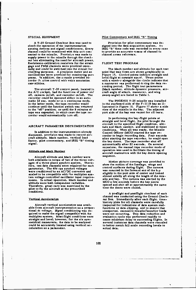
SPECIAL EQUIPMENT Pilot Commentary and IRIG "B" Tinning

A T-20 Ground Checkout Box wa« uaed to check the operation of the inatrumentation • enainf, device* and lignal conditioner». Every channel could be monitored with this ucit connected to the misaile. Provision was made to supply power to the missile through the checkout box eliminating the need for aircraft power. Resistance-calibration resistor» for the strain gage and FMM channels were provided inter- nally and could be switched into the circuit for checking purposes. A precision meter and an oscilloscope were provided for monitoring purposes. Tn addition, the console provided re- cordev faction control with voice annotation capMiilities.

The aircraft T-20 control panel, located in the A/C cockpit, had the functions of power on/ off, camera on/off, and recorder on/off. The recorder could be operated either in an automatic 22 sec. mode or in a continuous mode. In the latter mode, the Upe recorder would continue until the function switch was returned to the "off" position, or until the 8 minutes of tape w».s expended, in which case the tape recorder would automatically tarn off.

AIRCRAFT PARAMETER INSTRUMENTATION

In addition to the instrumentation already discussed, provision was made to record aircraft altitude. Mach number, vertical load factor, pilot commentary, and IRIG "B" timing signal.

Altitude a imbsr

Aircraft altitude and Mach number were both available in terqns of two of the three voltages of a three phase synchro system. There- fore, two data channels were required for each parameter. The 40U cps svnehro voltages were conditioned by an AC/DC converter and scaled to be compatible with fhe multiplex system voltage controlled oscillator input requirements. In actual operation. Mach number and altitude were both independent variables. Therefore, great care was exercised by the pilot to fly the aircraft at the prescribed conditions.

ttion

Aircraft vertical acceleration was available from aircraft instrumentation as a proportional dc voltage. Signal conditiouing was required to make the signal compatible with the multiplex system. Most flight conditions were straight and level; however, for the six sym- metrical maneuvers, the data to be analyzed could be accurately located using vertical acceleration as a parameter.

Provision for pilot commentary was designed into the data acquisition system. An IRIG "B" time code was recorded in every case to provide an accurate means of channel to channel cross reference.

FLIGHT TEST PROGRAM

The Mach number and altitude for each test point that was llown are shown graphically in Figure 15. Circled points indicate straight and level flight at constant speed. Those points with a numb' r alongside the circle indicate that a maneuver -vas performed dvring the data recording period. The flight test parameters (Mach number, altitude dynamic pressure, aircraft angle of attack, maneuver, and wing sweep angle) are listed in Table I.

The PHOENIX T-20 missile was installed in the starboard side of the F-111B bay as illustrated in Figure 16. Figure 17 show? a side view of the missile in the bay. The adjacent port side of the bay was vacant for All tests.

In performing the bay-flight points at straight and level flight, the pilot brought the aircraft to the specified flight condition, altitude and Mach number, and stabilised at these conditions. When all was ready, the Missile Control Officer (MCO) started the tape recorder to begin recording data. Four seconds after starting the tape recorder, he would open the bay doors. The tape recorder shut off automatically after 22 seconds. On several occasions, the manual tape recorder mode of operation was used to facilitate the timing of aircraft maneuvers with the bay doors opening sequence.

Motion picture coverage was provided to show the motion of the fuselage, wings and control surfaces during flight. The camera was mounted in the forward end of the b-y slightly to the port side of center and looked almost axially aft along the length of the missile and bay. The camera was started by the MCO a few seconds before the bay doors opened and shut off at approximately the same time the doors were closed.

A preflight and postflight checkout of each channel wes conducted using the Ground Check- out Box. Immediatsly after each flight, time- history plots for all channels were carefully inspected for indications of data system mal- functions or data clipping, and to ensure that unexpected, excessive missile/launcher loads were not occurring. This data reduction and evaluation cycle was performed rapidly to cause minimum delay to succeeding flights. In several instances data channels were rescaled to better match full scale recording levels to actual data.

102

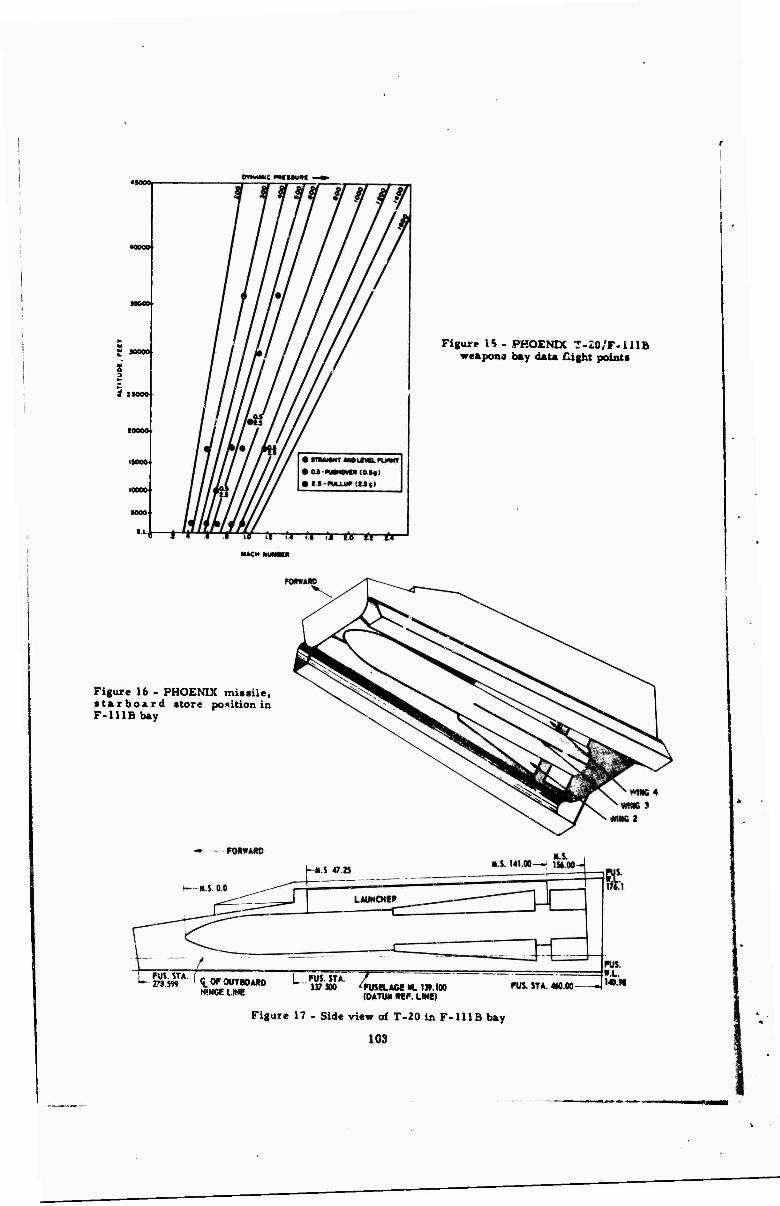
(mwauc nwuvn -

8

i »JOOO

•0004

i.i.

Figure 15 - PHOENIX T-20/F-U1B weapons b»y dau flight point«

•UCH NUMt*

Figure 16 - PHOENIX mittUe, • tarboard atore position in F-lUBbay

^TA' (q.«-_OUT«*«, L^^" ^aAC« ^ m.,0. HINCE LINE

Fü$. STA. 4M.03 4,mn

(DATUM REC. LINE)

Figure 17 - Side view of T-20 in F-111B bay

103

VOLTAGE CONTKOLLEO OSCILLATORS (VCO)

Figure 13 - Bottom view of multiplex system/ tape recorder assembly

Figure 14 - Top view - multiplex system/ tape recorder assembly

104

The F-lUB bay test flight» were flown out of the Hughe« Aircraft Culver City, California facility. Chase plane coverage was provided by the Navy facilities at Point Mugu. Missions were flown on the Point Mugu Test Range and the Edwards AFB Supersonic Range. The measurement system performed excellently in field usage resulting in a very successful 90% data retrieval for the entire flight program.

On several occasions throughout the flight test program, various channels of data were lost. However, because of the rigorous post flight checkout and quick look procedures, re- placement and repairs could be made before the next flight.

Post Flight Data Reduction and Evaluation

A more detailed data redaction and evaluation phase was performed after all flight tests were cotupleved. For a description of all he measurements, their d«ta reduction and their data evaluation, one is referred to Refs. 1 and 2. Ref. 2, a paper to be presented at the 39th Shock and Vibration Symposium by Curtis and Tinling, examines the degree of agreement between the predicted and measured vibration environments. In this paper the unsteady pressure measurements are presented and compared with those used for structural design.

PHOENIX BAY PRESSURE PREDICTIONS

A particularly difficult problem in the early design of the PHOENIX missile, was the establishment of open door design loads criteria for the missile in the F-1I1B bay. The criteria were needed to estimate an upper bound on oscillatory loads and vibratory responses in order to sice the missile and launcher structures.

Aircraft flight experience with the Falcon series of missile manufacture' Dy Hughes Air- craft Company had shown that a severe vibration environment often exists in a weapons bay when the doors are opened. Visual examination of accelerometer and strain gage traces had shown that bay mounted structures tend to be most highly excited at their lower structural frequencies and to respond with high stress levels. It seemed likely that the forcing frequencies must form a continuum, so that all structures placed in a bay would vibrate.

The engineering significance of the problem is that bay mounted missiles vibrating rapidly at relatively high stress levels, even for the short time the bay doors are open, may undergo a large number of oscillations and thus may accumulate significant fatigue damage. This fatigue environment, together with the peak response loads, tends to be of such significance as to ultirn&tely dictate the final design.

The task of establishing design loads criteria for the PHOENIX missile was made difficult since there were not. either from analyses or by past wind tunnel or flight measurements, sufficient information to accurately estimate either the rms values of the unsteady pressure excitations at locations within the F-111B bay or the power spectral densities and spatial correlations of pressures. Further- more, there existed so few unsteady pressure data for three-dimensional cavities and bays with missiles that confidence in simulation was low. and this discouraged the initiation of wind tunnel tests to obtain the unsteady pressure data on the PHOENIX/F-11 IB bay configuration. It was reasoned that if data were collected using small scale models, the applica- bility of the results to full scale missiles would be questionable. Full-scale flight tests of the missile in bays of other aircraft were considered, but found not feasible since the geometry of the aircraft in the vicinity of the missiles would need major and costly modifi- cations to simulate the local geometry of the F-11 IB aircraft.

As a result of these problems, it was de- cided to develop bay dynamic loads criteria for the PHOENIX missile utilising the empirical- analytical techniques ot Ref. 3. It was assumed that the principal source of vibratory loads in the F-111B bay would be the unsteady pressures in the bay. Consequently, design criteria were derived based on analysis of flight test response data for other captive bay missiles, and the analytical establishment of a pressure excitation acting over those missiles which produced responses compatible with their observed measurements.

As noted in Ref. 3, with one piece of response data to match (for example, the rms acceleration at the nose of a missile), one degree of freedom can be allowed in the description of the total fluctuating pressure acting on a missile. Thus, by selecting the spatial correlation of pressures as a fixed shape and by approximating the random precsures by white noise with a high cutoff frequency, an estimate of the fluctuating pressures acting on a captive missile can be derived from n, single response measurement. The reference suggested that mathematical models of missiles be analysed to find the level of the white-noiee spectrum.

To establish design loads criteria for the PHOENIX missile in the F-1I IB bay. strain gage and accelerometer data obtained during captive flight tests of previous HAC bay installed missiles {GAR-11 mis«ile/F-102 aircraft. GAR.3/F-106A. HM-55/J35F and GAR-i'J/F-IOlB) were analysed to estimate the ot dilatory bay pressures. Pressure magnitudes found in the above manner were plotted against dynamic pressure, as shown in Figure 18. Trends with q and bay configuration were investigated before selecting a white- noise pressure spectrum for PHOENIX design.

105

To thii apectrum were then added narrow-band level« at the estimated cavity resonant frequencies. The magnitudes of the narrow-band levels were estimated from the test data in Ref. 4.

Figure 19 shows the oscillatory pressure environment predicted for the PHOENIX in the F-111B bay. For dynamic pressures measured in psf, the level portion of the spectrum had a value in psiZ/Hz equal to 3.78 (10)-10 q2. Superimposed on this spectrum are shown estimates of the narrow-band spectral levels corresponding to the calculated bay resonant frequencies. The rms oscillatory pressures were predicted to vary linearly with dynamic pressure (q).

The pressure estimates were subsequently used to predict missile and launcher structural loads. The results are documented in Ref. 5. It was of interest, as the flight test program progressed, to compare the structural load and unsteady pressure predictions of the reference with those measurements by T-20.

UNSTEADY PRESSURE DATA REDUCTION

All unsteady PHOENIX T-20 pressure data reduction was performed using special purpose analog instruments which operated directly on the output voltage time history signals from the data recorders. The data were reduced into one or more of three different forms, as follows:

a) RMS values b) Power spectral density functions c) Cross correlation functions.

The purpose of measuring rms values for selected data channels was to obtain a rudimentary measure of severity (dispersion) for open bay dynamic data of interest. This measure of severity was needed to study relation- ships between selected open bay dynamic data (acceleration, pressure, and p*-iin) and pertinent flight parameters (dynan essure and Mach number).

Power Spectra-measurement«

The power spectra was measured from sample records which were formed into loops and recirculated to provide a continuous input to the analyzer. The sample records were selected during the time interval when the bay doors were fully open and the data were stationary. In most cases, nonstationary effects diminished immediately after the bay doors were fully open, permitting a four second long sample to be used. In a few cases, however, data were recorded during maneuvers which introduced additional nonstationary effects. For these data, sample record lengths were restricted to as short as 2 seconds.

Cross-Correlation Measurements

The purpose of the cross-correlation measurements was to establish the degree of similarity or statir.tical dependence between the measured unsteady pressures at different stations along the missile, and around the missile at the same station. Comparisons are made at various missile stations separated longitudinally and radially. The correlation coefficient was computed every one thousandth (.001) of a second.

RMS values were used as a rudimentary measure of dynamic severity for general data studies. Power spectra were employed to obtain a spectral decomposition of the data. Cross correlations were computed to provide information needed to check certain critical assumptions in the original dynamic load predictions for the PHOENIX missile.

RMS Vi'lue Meagurements

Thii rms pressure values were continuously recorded in real time during the interval when the bay door« were fully open and the data were stationary. This time interval was about 5 seconds long, which was ample for the volt- meter averaging circuit used for data reduction to fully respond to the data signals and produce unbiased rms estimates for the open bay environment. The lower frequency range of the instrumentation cut off at 2 Hz. This means that static levels (represented by a dc signal level) were not included in the measured rms values.

UNSTEADY BAY PRESSURE MEASUREMENTS

The validity of the assumption that the principle cause of vibration during open bay captive flight would be the aerodynamic ally induced fluctuating pressure field in the bay was readily substantiated by inspection of the data time histories before and after the bay doors were opened. It remained, however, to establish the relationship between the aerodynamically induced pressure field in the open bay and the aircraft flight conditions.

For "clean" or smooth structures moving through ambient air a turbulent aerodynamic boundary layer is produced whose magnitude and spectral characteristics have been fairly well defined by past theoretical and experimental studies. Specifically, the power spectrum for the pressure field, when suitably normalized, can be represented by a simple curve, as illustrated in Figure 20. For the problem at hand, the configuration was that of a missüe in an open bay, which is quite different from the idealized case discussed above.

106

10 I« 0.

^- u z a a

Figure 18 - Bay pressure magnitudes

SQUARE OF DYNAMIC PRESSURE, PSF2

2 W ^

I«

H U u

D w w u a a,

to ^7.56 H X3,7S

■

.

1

10 30 100 300 FREQUENCY, H«

1000

Figure 19 - Buy pressure spectrum predicted for all missile sections

Figure iO - Idealized pressure spectrum

107

In particular, the open cavity introduced acoustic resonances.

Inspection of the pressure transducer data revealed the presence of peaks in the pressure power spectra undoubtedly due to cavity resonances. However, the peaks were generally less than three to one. Even allowing for the suppression of the indicated peaks by the bias errors inherent in the d&ta reduction, it was clear that no unstable or strongly coupled cavity resonance occurred.

The next step was to determine if the power spectra for the pressure measurements would collapse to a curve similar to Figure 20 when normalised in a similar way. (In Figure 2u. P(f) is pressure spectral density, f is frequency, U is free-stream velocity, q is dynamic pressure, and 6* is boundary layer thickness.) If so. there would be strong evidence that the measured pressures were due to boundary layer turbulence, or something directly proportional to it.

The difficulty was to choose normalizing factors to apply to the bay data. It was de- cided to replace the parameters U, q, 6* by V, q, D (V is aircraft speed, q is dynamic pressure, D is transducer diameter).

The pressure data for all pressure transducer and microphone measurements for straight and level flight conditions were normalized as shown in Figures 21 through 24. In these figures, rma pressure values are shown plotted against dynamic pressure with a regression line fitted to the data. The normalized pressure spectra are presented as a spread where the gray area is the range of the maximum to minimum values observed at each frequency, and the dark line is the approximate mean of the values observed at each frequency (note that tne mean is not necessarily the middle of the range). Keeping in mind the random errors introduced during the data reduction, it is seen that the pressure data do scale reason- ably well using the variables of boundary layer turbulence. Had the pressure data been due principally to strong modal resonances of the cavity, the spectra would not have collapsed as well as they did.

The pressure data were also investigated for a Mach number dependence. This was done by dividing the rms pressure values by q and plotting the resulting normalized rms values versus Mach number. In «om» cases, slight trends of rms/q appeared to be present, but the trends were not considered significant compared to the data scatter. A summary table of rms pressure levels is presented in Table 1.

On the basis of the above studies, it is concluded that the pressure field in the bay is due primarily to random boundary layer pressure driving many acoustic modes of the cavity. The amplitude of the measured rms pressure is

approximately 10 to IS db higher than that predicted by flat plate theory, but this can be accounted for by the resonant amplification by the cavity modes.

The pressure spectra for the microphones were generally processed only to 2000 Hz. The data were checked above 2000 Hz, and displayed a characteristic rapid drop off to 10,000 Hz.

Data were also measured for closed aircraft bay doors, but were not processed, however, due to their extremely low magnitudes.

An evaluation of the pressure data was performed using cross-correlation analysis. For the original missile load predictions, it was assumed that the pressure field acting on the missile structure was perfectly correlated (a correlation coefficient of unity at zero time delay) from one point to another. It was of interest to check the validity of this assumption using the actual measured pressure data. Such checks were made by computing the cross- correlation coefficient for the pressure measurements between various selected points. The results are presented in Figures 25 and 26. Definite correlation was exhibited between the pressures at stations 131.62 and 151 on the left side of the missile (a separation of 19.38 inches). The correlation coefficient was 0.3 5 for one flight and 0.2 for another. In both cases, the correlation peaks occurred at a time delay of about ±3 milliseconds. This means that from 20% to 35% of the excitation power at station 131.62 appeared some 3 milliseconds later at station 151, and vice versa. The correlation peaks are approximately sym- metric about zero time delay. The cross- correlation function between the pressures at two points in a turbulent boundary layer on a smooth structure would generally be asym- metric about zero time delay. This implies that, although the boundary layer was the basic source of excitation, the pressure fiald inside the bay cavity was significantly modified by the acoustic resonant modes of the cavity.

Referring again to Figures 2 5 and 26, significant correlation was also exhibited between the pressures on the bottom anJ the right side of the missile at station 3 5.7 (a separation of 11 inches). The coefficient was about 0.3 with a zero time delay. This indicates that the pressure field was instantaneously correlated at points around the circumference of the missile at any given station, as would be expected.

The other measured cross-correlations were for points separated by 50 inches or more. No significant correlation peaks are indicated. In summary, it appears thai the spatial correlation characteristics of the pressure field on the missile diminished with distance to a correlation of about 0.3 at 20 inches separation, and to a negligible correlation coefficient at more than 50 inches separation.

108

»

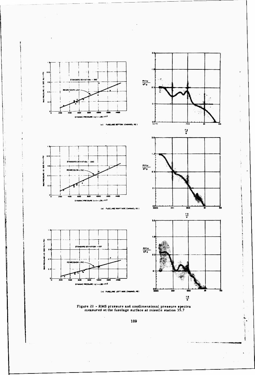
muuw (m-LWn»

I» ruWuwiiwtMtiawwfiW!

8 " i

I

— — —

r*i MXOKV

\

UTIM • 037

• naacuio« .1«

P^ ^

-H"^ **

MO »oa loco nee

orMwcMnuxc i«i-LK'n'

>tl FUMUMI Lift «MSCMUMLMI

l_0 V

Figure 21 - RMS pressure and nondimensional pressure spectra measured at the fuselage surface at missile station 35.7

109

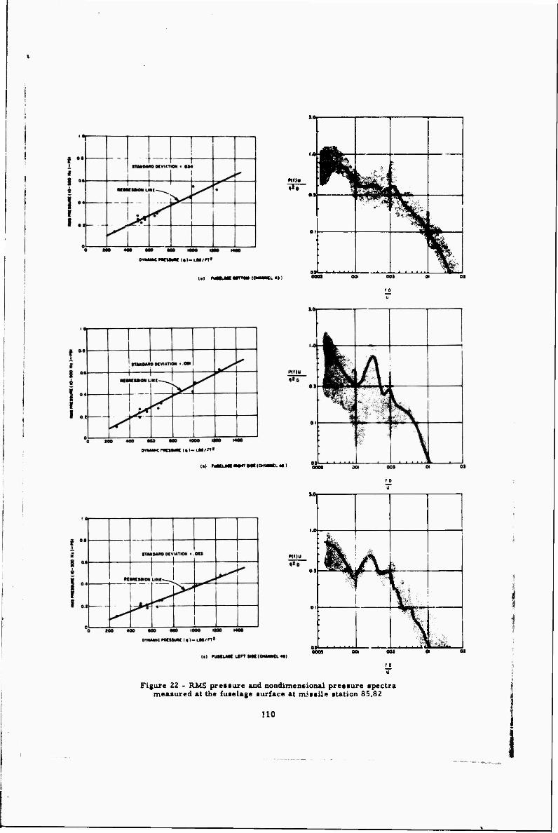
l«l-LM/nl

10

M

f II bfei 1 L ^■:^5fl •\ id

^fej SI « L |

' K 1 '^K

01 1_ . _ Wll

aoi

f o

Dn««n«nuw i«i-LM'rrt

(tl niMLMIMwrMI(OMIIMLW) gjo,

10

0>

01

ot

A 1

i ^

1 1 J i^Ä 1

— u

Figure 22 - RMS preasure and nondimentional pressure spectra measured at the fuselage surface at missile station 85.82

110

Ki nmum mrnm lo—t.«" i

\

. tTWOMO DC

1 IITIM • 09T

^ « MCmOk u»t , ^N. ^

y^

^^ -^^7' - - < j

0 ^ ,., .

•OD MO

ikl ru|<tl.MilMMTII(0e(CMMMIL4n

f 0,

i

9 aa

ITUMII D DCVItr M ■ OM

u^

**

8 •• M« €5*051 L ist ^

f^ ^

r

•

^ 1 .,_!

5» 1000

onuiicMmuw -ai-Lnm'

icl ruMUMl iirr UMICMMMCLHI IS u

Figure 23 - RMS pressure and nondimensional pressure spectra measured at the fuselage surface at missile station 131.62

111

I

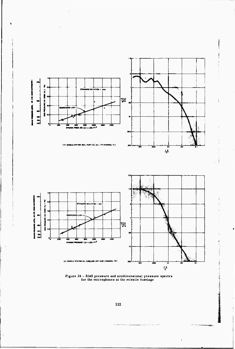
i:

<•! mtmiM www »». miua«»i■>« lon—ctni

1

\s> ■\

1

.01

001

.001

\

\ >

\

U j . .1.1. 1 -_.

(«t-L^•/rr•

l» MUILI <T>7H» III, ruHlMI LITT »DI (CMWOIL rtl

10

ti?^.>t

^ 1 \

M

■

|

•

k 01 J» .0 00 .0 1 0 s a

Figure 24 - RMS pressure and nondimensional pressure spectra for the microphones at the missile fuselage

112

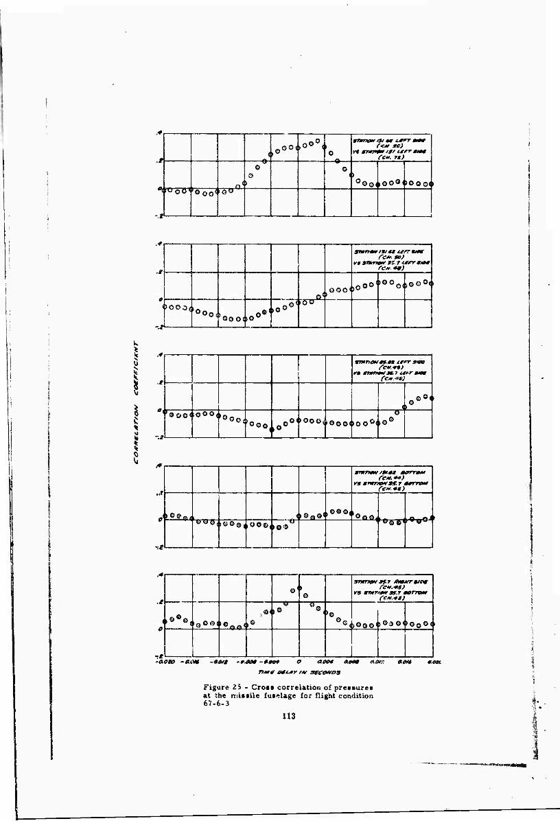
v* sntnm» i3f terr att Ce-. *z)

0 o

O i 1

OO0IIGOOI>OOGM rcTööi 'OOO«'©«'

—i

rc te) v* snna* SS 7 nsrrstow

OOO (»O' oo'X'Ooo©000

DOOOo ÖSTT

GO Od> oo1

-^ ooooo

k

\

.*

.*

sntrtof »g.m irrr »m

if» annmwßt.7 itt-r sum

„©©( ! 4° «1

-.9

'©OOi iOOO, •oo0i iOoo( 1© »0O©j iOOO« »000(

0 .0°

~.s

10© jgui ^^Oo«©© (|0«©(i©0

©0©<lGeo<'

smntmi/ms* morrmmi rs smrm/as.r mtnttnn

^^'Ooftl^^©-"

(.«»«© (Ig @0OO

•5« -AC«? -«<Wf

oo

,®o

vs siMTra*sr.r scmuf

i>000©03Qi>©00(i

-««W» -#^M» -<*««# 0 O^MI «««

Figure 23 - Crocs correlation of pressures at the missile fuselage for flight condition 67-6-3

113

*•

u0 ooooooooooo G O ©O OA

CCM. SO) ft snr/OM 'i i it*r s,o*

(en rt)

GG. (IG GG »no00

-J

-a

tr5^< > G 0 o (>GGoiG00<» G G 0 < »O©© QOOOQ

STXTIOMm*a irrr t/ot fen. so)

v% smTioM M.7 tt'rtios

-OWS <M^ (10 G-&4)

I ■smr/oiv «fM terr sroe

fCM *») vs snnon Sf.7 ctrrsioi

rcM. 0»)

>000( »OG-, .O0O ^oo, GO« IG 0©. 'mQ0'

OoO( >ü ö0< (G© ' 1 O

1*

■t

( 0

-.2

smnoM sf.tt trrrsioe fcM. *a )

VS snr. W 55.7 sorroM fe*. *t)

000( © o' 0oo< ,oOe< ,0GG^ • ©o0-? ,000« •©©o« • GO©« ,0G©<

...

i

< 1

STtriCM Si 7 l»6MTSIO€ (■CM. *S)

vs srjirtoM ss- 7 ocrrroM (en **)

>©o0< O©©, ,OOo< ,00°

Ho 0 o©< •oo0) ,000, »000( 'Oo©'

e aoo* too» TTMt oct*r/*/ »teoA/oa

Figure 26 - Cro»» correlation of pressure« at the missile fuselage for flight condition 67-9-5

114

■

■

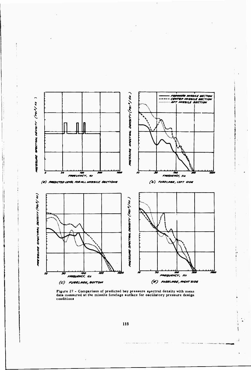
r-i n n

1

■

^

(a) ßmafcfWtum *o**u. AMSSHS smcrroHm

\

\

(c) tvsei/Hfe, morrot*

Figure 27 - Comparison of predicted bay pressure spectral density with mean data measured at the missile fusslage surface for oscillatory pressure design conditions

115

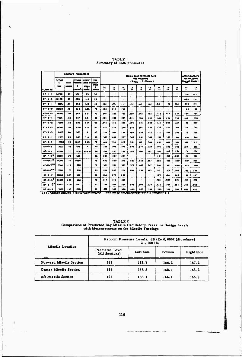
TABLE 1 Summary of RMS pretsures

ruetrao.

«murT nuMHCTi« ntuu» MM mtstwK MT« ■CmMMUT«

ÜTiTyM h

nrr Z. wmtp mmM A

«tl MCUMC nian II-SOOHII

mamatum PJ^^S-IOOOM-l

■mcM CI« «a

CM «s

CM 4*

CM CM 4«

CM 4?

CM «• 4t CM M

CM CM n

• T-l-l »7*0 •T 100 49 90 - ~ - ~

- - -r- 07t .u?

•r-i-i into to too 4.1 M - - - on 114

•r-t-i (OK .4t no !.• M ill 199 Ht

IM

.IM

.192

.114

Ill 101 .091 .102 .191 ot« 114

n-t't IMW 1.10 SIS 7.M 7t .119 .114 - - - - .140 Itt

tt-t-» 1 JO iti t.S7 71 t4S .249 249 .IM Ill .179 .114 .11« .111

W-J-l irooc M »97 S.S SO .IM tu

91«

.114

.its

.114 .199 .199 .149 .104 ISS Itt | .190 j

•T-S-l 17000 .M «M It 90 .149 m .91t .199 .179 .149 .997 IM IM

•T-»-J 10000 .?0 soo I.« 90 114 179 140 tu

.i««

.MT

MS

US

.41t

.199 .199 114 .90« It« i .t«o

•r-s-» MOO .M soo .• SO IM

.997

.410

199

149

.491

910

m

IM

9t7

.41t

149 - IM

.17» 1« IM 149 172 12t

•r-«-i tow ,M tM 9.« so

71

.IM IM 917 1 .910 104 IM

«r-»-s «000 n IMS IM .911 til

.149 1 .179

.199 [ .IM

94t .41t 4M Ml .944 910

«-•-» tooo 70 *7S .t

• •a

so 114 1 .199 149 90t 114 Itt

«r-r-i 70 SOO 1«

tl

IM

104

.tn

991

SV*

.tM

9t7

»"I :* t«9

179

.IM Kl« IM IM .174 ' .2M 1

«r-r-s» .70 300 ... ;

104 .IM i IM 10000

.970 .990

.971

IM

»5 •T-«-I» IKOO I.I« 1010 71

71

«99 M7 .41« .910 .470 i .419

«■•f irooc 1 IS 1020 3«7 — - -

104

M3 —

IM

.M7 : ist 1 .it9 ; .in

977

IM

.410

.MS

499 IM

•T-t-l»* inooo .70 900 1« '« IM

•r-»-» IOS MO 71 IM 190

JOt

.194

.9M

.24t IM MO 12ÜÜÜ " .L "_. «-«-»• Jäooo 10» MO 71 .114

.IM

.91t

.tt9

.400

its

900

- ■ .IM IM 279 l» .17»

«r-t-r HOQO I.Ot MO 71 IM t

.97«

113 210 1(1

.9M .240 •T -»-s 11000 I.IS 10» 7J 971 MO 900 4W 491

«os< nOM WtKMW CUVCR •«t s« «JLLUH uwuvr • • • MTAM IT4VIML« uimr UtHTt« -7-1 INI lOMNff? -»-9

TABLE 2 Compariton of Predicted Bay Mittile Oscillatory Pressure Design Levels

with Measurements on the Missile Fuselage

Missile Location

Random Pressure Levels, dB (Re 0.0002 Microbars) 2 . 500 Hz

Predicted Level (All Sections) Left Side Bottom Right Side

Forward Missile Section 165 162.7 166.2 167.2

Center Missile Section 165 165.8 168.1 168.2

Aft Missile Section 165 168.1 i66. 1 166.9

116

The pressure data in Table 1 shown that forward of the wing, high rms prer/turea occur on the side of the missile near the bay wall«. whereas aft of the wing the high rms pressures occur near the bay centerline. For straight and level flight, the pressures on the missile adjacent to the bay opening were usually greatest near the forward wing attachment. In all cases, pushover maneuvers caused these pressure levels to increase. The microphone data showed higher pressure readings usually occurring fit the aft portion of the missile radome bulkhead near the bay opening. Photo- graphs of the tufts within the bay indicated for many flight conditions forward flow within the bay near the bay floor.

COMPARISONS WITH PREDICTIONS

The measurements during these flight tests provided data needed for the refinement of initial unsteady pressure predictions and the upgrading of missile and launcher structural design criteria. The oscillatory pressure environment for design of the PHOENIX in the F-1UB bay is illustrated in Figure 27a. Fig- ure 27b, c, and d show measured pressure (spectral density data, extrapolated to the same design condition. The data tend to be much higher than the predicted levels at the low frequencies, and drop off to lower levels at the higher frequencies. In the frequency band of major fuselage reconances, the measured oscillatory pressure spectra are generally 1.5 to 2 times the predictions. Overall random pressure levels are compared in Table 2 for a selected condition. The levels change with location on the missile, but generally they are quite close to the predicted overall level.

In general, there was basic agreement between dynamic loads measured and predicted. Errors in predicting the magnitude and spectral density of the pressures alcng the missile for loads studies were compensated by conservative estimates for the spatial coherence. The bending and torsion loads on the control surface near the bay floor and centerline were 10-15% higher than predicted while the measured values on the other three control surfaces were generally less than predicted. The resultant of the vertical and lateral fuselage bending moments were close to predicted moments. A direct comparison of predicted and measured wing bending moments could not be made since the measurements were taken on a wing whose fuselage attachment was different from that analysed. No structural damage to the missile occurred during the flight test program even though the tc .1 time the bay doors were open was several times that required for missile design.

CONCLUSIONS

in the weapons bay of an F-l 1 IB aircraft, the approach used to make early estimates of the fluctuating pressure field, and the recent measurements . The major conclusion« are as follows:

1. The design concept of the PHOENIX missile measurement system being self- contained and dependent on the mother aircraft only foi power and on/off control was proven to be a good approach.

2. The PHOENIX T-20 bay measurements program was highly successful in both quantity and quality of data acquired.

3. The criteria used to predict the unsteady pressures in the F-l 1 IB bay and to establish PHOENIX design loads were adequate for that design but may not apply for other missiles or other bays.

4. A more refined analytical-experimental approach needs to be developed to estimate the dynamic loads and vibratory responses for missiles housed in an open weapons bay.

ACKNOWLEDGEMENTS

The writers of this report wish to acknowl- edge the help of those members of the Space Systems Division, Flight Test Division, Aero- nautical Systems Division, and the Missile Systems Division of Hughes Aircraft Company who contributed to the success of this program.

REFERENCES

!. ,,XAIM-54A T-20/F-111B Weapons Bay Environmental Measurements Post Flight Evaluation Report" by T. M. Kiwior and R. P. Mandich, TPM Section R-3. 3. 2. 3.1, 1 April 1968.

2. "Success and Failure with Prediction and Simulation of Aircraft Vibration" by A. J, Curtis and N. G. Tinling, Shock and Vibra- tion Bulletin 39 (to be published).

3. "Captive Missile Response Due to Random Pressures" by H, L. Leve, pg. 698-709, from Symposium Proceedings: Structural Dynamics of High Speed Flight, ACR-62, Volume I, Aerospace Industries Associated {Office of Naval Research), Los Angeles, California, April 1961.

4. "A Theoritical and Experimental Investi- gation of the Acoustic Response of Cavities in an Aerodynamic Flow", WADD-TR-61- 75, byH.E. PUtmbee, J. S. Gibson, L. W. Lassiter, March 1962.

5. "PHOENIX Missile Response Report" by R.J. OedyandJ.B, Yows, PMS-49/2222, July 1965 (Conf).

The paper has described the captive flight measurements program of a PHOENIX missile

117

DISCUSSION

Mr. Mustaln (McDonnell Douglaa Corp.): The questloD I have ia on correlation. Did you make a check to see what happened to the vibration responses in the missile along with the correlation? For instance, if you had a correlated field, were the vibration levels greater or could you make any distinction there at all?

Mr. Mandich: Are you talking about the measurements or Uie original predictions?

Mr. Mustein: The actual measurements - not the predictions. Did you have a higher vibration level on your accelcrometers in a correlated field or an uncorrelated field?

Mr. Mandich: We measured the correlation that actually occurred in the uay. The correlation was about 0.3 for close separations and then it dropped off with distance. We were using actual measurements so we did not have fully correlated or fully uncorrelated fields.

We did the original analysis from missile loads- we maoo those two limiting cases.

Mr. Mustaln: You still did not answer my question. In correlation studies it is quite often said that in most cases the response is with a correlated field. But this is not always the oj^e and here you have an example of actual measurements. TZ is hard to find actual measurements of cvrrelsted fields and check against the vihralioii. You have a vibration data, and you have measurements for the acoustic cor- relati/rc. You can look at die data to see if the correlated field or the uncorrelated areas give you a greater response.

Mr. Mandich: check.

We have not gone back to

Mr. Mustain: I would suggest you do it and I would certainly like to know how your answers come out.

118

L

LUNAR ORBITER FUGHT VIBRATIONS WITH COMPARISONS TO

FLIGHT ACCEPTANCE REQUIREMENTS AND PREDICTIONS BASED ON

A NEW GENERALIZED REGRESSION ANALYSIS

By Sherman A. Clevenson NASA Langley Research Center Langley Station, Hampton, Va.

This paper .resents detailed flight-measured vibration data obtained during the five successful flights of the Lunar Orbiter and compares these data with vibration levels specified as flight acceptance requirements. These data are also compared with predictions based on results of a recently developed regression analysis of vibration data compiled for a number of major launch vehicles. It is shown that the flight acceptance requirements were adequate but due to unexpectedly low random vibration flight inputs, the random acceptance requirement is considered severe. For establishing vibration requirements utilizing a proven launch vehicle, the regression analysis does not provide as good as a basis as does flight vibration measurements from prior flights of the launch vehicle. However, the regression analysis may be useful in estimating vibration levels for new and untried launch vehicles.

INTRODUCTION

Five successful Lunar Orbiter spacecraft were launched during the period of August 6, 1966, through August 1,1967, whose mission was to secure topographic data of nearly all of the moon's surface. Prior to their flights, the spacecraft underwent qualification and flight acceptance tests. During their flights, the spacecraft were subjected to environmental inputs from the launch vehicle, one of the most severe being vibration. During each flight, vibration measurements were continuously obtained using accelerometers which allow the determination of peak vibrations for critical conditions of lift-off, transonic speeds, booster engine cut-off, booster engine staging, sustainer engine cut-off, vernier engine cut-off and hori- zon sensor fairing ejection, shroud jettison, Atlas-Agena separation, Agena first and second ignition and burnout, and spacecraft separation.

The purpose of this paper is to present results of the analyses of the flight vibration measurements and to compare these data to flight acceptance test requirements. In addition, these data are compared with the results of a recently developed regression analysis technique for predicting random vibration levels for any spacecraft.

SYMBOLS

a indication of low signal amplitude or less than 2 cycles for frequency analysis

b indication ol no available data

c indication of a pulse peak amplitude

d indication of the changeover from accelerometers to position indicators

cr

damping

critical damping

f frequency, Hz

FAT flight acceptance tests

g acceleration

Speak Peak acceleration

gp.p double amplitude acceleration

g2/Hz acceleration squared per Hz

G(f) average power spectral density;

119

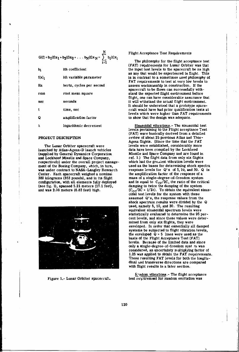
G{£) = biWxj N

fb2(f)x2+ • • • 1^(0x1,}= 2^ i=l

bl 1th coefficient

fWi ith variable parameter

Hz hertz, cycles per second

rms 1

root mean square

sec seconds

t time, sec

Q amplification factor

\ logarithmic decrement

PROJECT DESCRIPTION

The Lunar Orbiter spacecraft were launched by Atlas-Agena-D launch vehicles (supplied by General Dynamics Corporation and Lockheed Missile and Space Company, respectively) under the overall project management of the Boeing Company, ivhich, in turn, was under contract to NASA-Langley Research Center. Each spacecraft weighed a nominal 380 kilograms (853 pounds), and in its flight configuration, with all elements fully deployed (see fig. 1), spanned 5.21 meters (17.1 feet), and was 2.08 meters (6.83 feet) high.

Figure 1.- Lunar Orbiter spacecraft.

Flight Acceptance Test Requirements

The philosophy for the flight acceptance test (FAT) requirements for Lunar Orbiter was that the input test levels to the spacecraft be as high as any that would be experienced in flight. This is in contrast to a sometimes used philosophy of FAT requirements to test at very low levels to assess workmanship in construction. If the spacecraft to be flown can successfully withstand the expected flight environment before flight, one can have considerable assurance that it will withstand the actual flight environment. It should be under stood that a prototype spacecraft would have had prior qualification tests at levels which were higher than FAT requirements to show that the design was adequate.

Sinusoidal vibrations.- The sinusoidal test levels pertaining to the Flight acceptance Test (FAT) were basically derived from a detailed review of about 25 previous Atlas and Thor- Agena flights. (Since the time that the FAT levels were established, considerably more data have been compiled by the Lockheed Missile and Space Company and are found in ref. 1.) The flight data from only six flights which had the grt^test vibration levels were used as the bases for determining shock spectra response levels for Q' s of 5,10, and 30. Q is the amplification factor of the response of a mass of a single-degree-of-freedom system and is equal to Ccr/2C, the ratio of the critical damping to twice the damping of the system (Ccr/2C = 1/2X). To obtain the equivalent sinusoidal test levels for the system with these assumed Q1 s, the response values from the shock spectrum results were divided by the Q used, namely 5, 10, and 30. The resulting equivalent sinusoidal spectrum levels were statistically evaluated to determine the 95 percent levels, and since these values were determined from only six flights, they were enveloped. In order that essentially all damped systems be subjected to flight vibration levels, the enveloped Q = 5 lines were used as the basis of the Flight Acceptance Test (FAT) levels. Because of the limited data and since only a single-degree-of-freedom syst m was considered, an uncertainty multiplying factor of 1.25 was applied to obtain the FAT requirements. These resulting FAT levels for both the longitudinal uid transverse directions are compared with flight results in a later section.

K^adom vibrations.- The flight acceptance test retirement for random excitation was

120

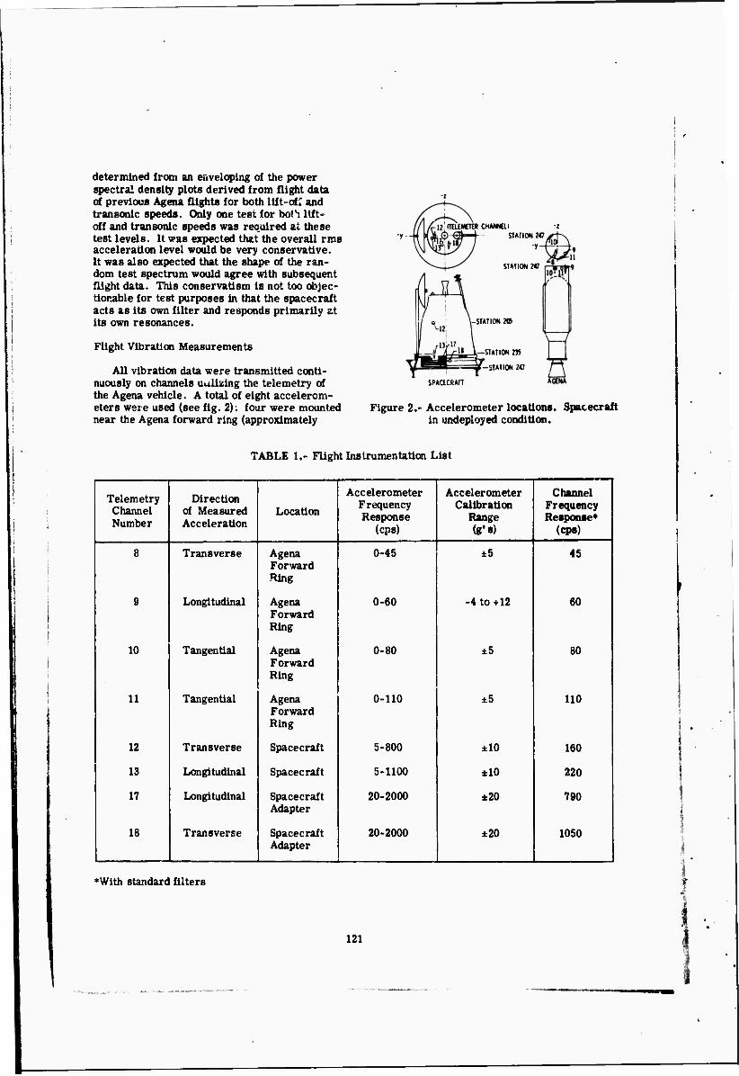
determined from an enveloping of the power spectral density plots derived from flight data of previous Agena flights for both Uft-of: and transonic speeds. Only one test for both lift- off and transonic speeds was required at these test levels. It was expected that the overall rms acceleration level would be very conservative. It was also expected that the shape of the random test spectrum would agree with subsequent flight data. This conservatism is not too objec- tionable for test purposes in that the spacecraft acts as its own filter and responds primarily zt its own resonances.

Flight Vibration Measurements

All vibration data were transmitted continuously on channels uulizing the telemetry of the Agena vehicle. A total of eight accelerometers were used (see fig. 2): four were mounted near the Agena forward ring (approximately

(TELEMOIR CHANNai STMION 247

STATION 247

-STATION 205

''j- l—STATION 235

p-STATION 247

SPACtCRAfT A'

Figure 2.- Accelerometer locations. Spacecraft in undeployed condition.

TABLE I.- Flight Instrumentation List

Telemetry Channel Number

Direction of Measured Acceleration

Location

Accelerometer Frequency Response

(cps)

Accelerometer Calibration

Range (g's)

Channel Frequency Response*

(cps)

8 Transverse Agena Forward Ring

0-45 ±5 45

9 Longitudinal Agena Forward Ring

0-60 -4 to +12 60

10 Tangential Agena Forward Ring

0-80 ±5 80

11 Tangential Agena Forward Ring

0-110 ±5 110

12 Transverse Spacecraft 5-800 ±10 160

13 Longitudinal Spacecraft 5-1100 ±10 220

17 Longitudinal Spacecraft Adapter

20-2000 ±20 790

18 Transverse Spacecraft Adapter

20-2000 ±20 1050

»With standard filters

121

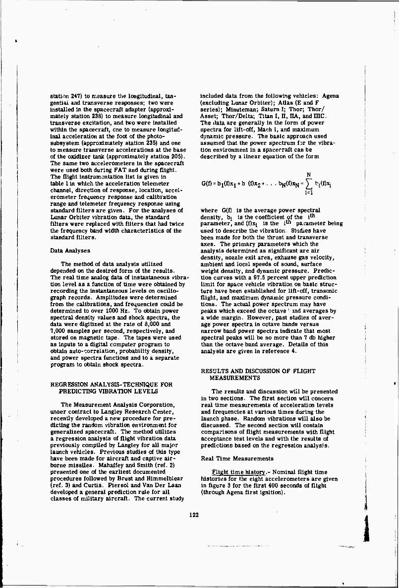
station 247) to measure the longitudinal, tangential and transverse responses; two were Installed in the spacecraft adapter (approximately station 238) to measure longitudinal and transverse excitation, and two were Installed within the spacecraft, one to measure longitudinal acceleration at the foot of the photo- subsystem (approximately station 235) and one to measure transverse accelerations at the base of the oxldizer tank (approximately station 205). The same two accelerometers in the spacecraft were used both during FAT and during flight. The flight Instrumentation list is given In table 1 in which the acceleration telemeter channel, direction of response, location, accelerometer frequency response and calibration range and telemeter frequency response using standard filters are given. For the analyses of Lunar Orblter vibration data, the standard filters were replaced with filters that had twice the frequency band width characteristics of the standard filters.

Data Analyses

The method of data analysis utilized depended on the desired form of the results. The real time analog data of instantaneous vibration level as a function of time were obtained by recording the Instantaneous levels on oscillograph records. Amplitudes were determined from the calibrations, and frequencies could be determined to over 1000 Hz. To obtain power spectral density values and shock spectra, the data were digitized at the rate of 8,000 and 7,000 samples per second, respectively, and stored on magnetic tape. The tapes were used as Inputs to a digital computer program to obtain auto-correlation, probability density, and power spectra functions and to a separate program to obtain shock spectra.

REGRESSION ANALYSIS-TECHNIQUE FOR PREDICTING VIBRATION LEVELS

The Measurement Analysis Corporation, unoer contract to Langley Research Center, recently developed a new procedure for predicting the random vibration environment for generalized spacecraft. The method utilizes a regression analysis of flight vibration data previously compiled by Langley for all major launch vehicles. Previous studies of this type have been made for aircraft and captive air- borne missiles. Mahaffey and Smith (ref. 2) presented one of the earliest documented procedures followed by Brust and Hlmmelblear (ref. 3) and Curtis. Plersol and Van Der Laan developed a general prediction rule for all classes of military aircraft. The current study

included data from the following vehicles: Agena (excluding Lunar Orblter); Atlas (E and F series); Minuteman; Saturn I; Thor; Thor/ Asset; Thor/Delta; Titan I, II, HA, and mC. The data are generally in the form of power spectra for lift-off. Mach 1, and maximum dynamic pressure. The basic approach used assumed that the power spectrum far the vibration environment in a spacecraft can be described by a linear equation of the form

N G(f) = b1(f)x1 + b (f)x2+ . . . bN(f)xN= ^ bjWxj

where G(f) is the average power spectral density, bj is the coefficient of the i^1

parameter, and (f)xi is the i"1 parameter being used to describe the vibration. Studies have been made for both the thrust and transverse axes. The primary parameters which the analysis determined as significant are air density, nozzle exit area, exhause gas velocity, ambient and local speeds of sound, surface weight density, and dynamic pressure. Predic- tion curves with a 97.5 percent upper prediction limit for space vehicle vibration on basic structure have been established for lift-off, transonic flight, and maximum dynamic pressure conditions . The actual power spectrum may have peaks which exceed the octave ' ind averages by a wide margin. However, past studies of average power spectra in octave bands versus narrow band power spectra indicate that most spectral peaks will be no more than 7 db higher than the octave band average. Details of this analysis are given in reference 4.

RESULTS AND DISCUSSION OF FLIGHT MEASUREMENTS

The results and discussion will be presented in two sections. The first section will concern real time measurements of acceleration levels and frequencies at various times during the launch phase. Random vibrations will also be discussed. The second section will contain comparisons of flight measurements with flight acceptance test levels and with the results of predictions based on the regression analysis.

Real Time Measurements

Flight time history.- Nominal flight time histories for the eight accelerometers are given in figure 3 for the first 400 seconds of flight (through Agena first ignition).

122

1

^IF7affKco^c,Nc

rA-A StPARATION

SHROUO At, MfcNA FIRSI vao-A/N^11""«"

SECO--1 m X' CHAWB. ■ " 12

ACCaERAIK». 9

CHANWL DIRtCTION

- » TSANSVtHa

- 9 lONCITUDINAL

- 10 lANKNTIAL

13 lONOITUOIN/U.

17 LONCITUDIKAL

18 TRANSVERSE

Figure 3.- Nominal flight time history.

The time scale is too compressed for accurate analyses of the data. However, the responses are as expected with bursts of acceleration occurring on the record. Some of the significant flight events are indicated. The traces are identified by telemeter channels which are listed in table 1, Channels 17 and 18, the longitudinal and transverse accelerometers in the adapter, were responsive to the higher frequencies and indicated the largest vibrations. Acceleration magnitudes and frequencies obtained from high-speed oscillograph recordings will be discussed in the next section.

Peak vibration levels at significant events.- During the launch piiase of the Lunar Orbiter flights, vibration levels and predominant frequencies were determined for the following events:

Lift Off Transonic Speed Booster Engine Cut Off (BECO) Booster Engine Staging (BES) Sustainer Engine Cut Off (SECO) Vernier Engine Cut Off (VECO) and Sensor

Fairing Jettison Shroud Jettison Atlas-Agena Separation Agena First Ignition Agena First Burn-Out Agena Second Ignition Agena Second Burn-Out Agena Lunar Orbiter Spacecraft Separation

From table 2, it may be noted that peak vibration levels and response frequencies are rea- sonably similar for these events from flight to flight for the five flights of Lunar Orbiter.

Figure 4.- Response at Atias-Agena separation. Lunar Orbiter V.

Figure 4 shows the representative responses of the accelerometers on Lunar Orbiter V at Atlas-Agena separation. It should be noted that 1000 cps oscillations and below may be easily determined. The peak-to-peak and pulse acceleration levels are determined from the calibrations. It is apparent from this representative example that only a few cycles of oscillation are available for determining response frequencies. The top four traces on figure 4 are good examples of pulses. In some Instances, flight data were not available due to lack of appropriate flight magnetic tapes or due to electronic difficulties either in the original tapes or in the recovery of the data. For example, on the flight tapes of Lunar Orbiter I from all receiving stations there were no data on channel 12 until the channel was switched to another transducer. Prior to Agena-Lunar Orbiter spacecraft separation, telemeter channels 9, 12, and 13 were switched to dash-pot type position indicators to record the spacecraft separation. Thus, no vibration data were recorded for this event on these three channels. In addition, since the telemeter was in the Agena, no further vibration information was available from the spacecraft.

Random vibrations.- From figure 3, it was noted that high vibration levels for more than a few seconds occurred at lift-off and then again at times 55 to 65 seconds of flight. These levels are attributed to random excitation: at lift-off the vibration is attributed to acoustic coupling and at 55-65 seconds (transonic speeds) the vibration is attributed to aerodynamic buffeting.

Power spectral density analyses were made for telemeter channels 12 and 13 in the

123

i

TABLE 2 AmpLHudes and Approximate Frequencies of Flight Transients

Lunar Orblter I n m IV V |

\ ^"S. Item ChanneTS.

gp-p f gp.p f gp-p 1 f gp-p f gp-p f

| LIFT-OFF

8 2.5 3.0 1.4 5.5 0.5 a b b 0.6 5 9 0.7 a 1.6 42.0 0.5 a b b 1.1 5

10 1.0 a 0.9 82.0 0.5 a b b 1.0 a 11 1.0 a 1.2 570.0 1.5 a b b 1.0 a

! 12 b b 3.1 5.5 0.5 a b b 1.7 a

13 1.0 520 1.9 400.0 1.5 a b b 1.4 5 ! 17 14.0 1000 12.8 960.0 28.0 1000 b b 17.0 1000

i 18 14.0 1000 10.5 960.0 10.0 1000 b b 12.0 900 j

TRANSONIC SPEEDS

8 2.8 3.0 0.9 29.0 2.5 a 1.8 a 2.4 a 1 9 1.3 a 2.0 34.0 1.5 a 1.2 a 3.0 a I 10 1.0 56.0 0.8 a 0.5 a 1.4 a 1.0 a 1 11 1.3 91.0 0.6 a 0.8 a 1.0 a 1.3 a

1 12 b b 0.6 a a a 0.1 a 0.7 a 1 { 13 0.8 500 1.7 a 0.6 400 0.3 400 0.7 a

17 12.0 1000 8.8 960.0 26.0 1000 14.0 1000 17.0 1000 18 12.5 1000 6.5 960.0 1 .0 1000 7.0 1000 17.0 1000 1

BOOSTER ENGINE CUT-OFF j

1 8 1.1 9.9 0.1 62 a a 0.3 a 0.3 ^ 9 3.9 a 0.9 15 a a 1.2 15 0.7 a

10 1.9 66.0 0.9 63 1.0 64 1.4 61 1.7 65 ! ** 2.3 66.0 1.2 63 1.6 67 1.7 62 2.0 65

| 12 b b 0.5 a 1.0 a 0.7 a 0.7 a

1 13 3.0 1.2 0.7 34 1.0 a 1.4 59 1.4 19 1.5 16.0 1.9 14 1.0 a 1.4 59 1.4 19 1.0 65.0

i I7 0.1 1000 0.2 960 0.5 a 0.5 1000 1.3 a j 18 0.1 1000 0.4 960 0.5 a 0.5 1000 1.2 a

1 BOOSTER ENONE STAGING

8 0.5 a 0.5 38 0.5 a 0.6 a 0.7 38 I 9 0.4 a 0.5 32 0.3 a j 0,7 35 0.5 38

10 2.5 390 1.2 69 0.5 1 a 0.9 71 0.7 a U 3.0 390 1.0 35 0.9 a 0.8 71 i.O a

12 b b 1.5 35 1.0 a 1.4 35 1.7 34 13 1.0 a 0.5 444 0.7 400 1.4 35 l.l a 17 0.6 a 3.7 950 4.0 1000 1.7 1000 2.4 1000 18 0.6 a 1.4 950 2.0 1000 1,4 1000 1.7 a

124

TABLE 2.- Continued.

I

Lunar Orbiter I n m IV V

'v\Item Channei\.

Bp.p f VP f BP-P f VP f VP f

SUSTAINER ENGaNE CUT-OFF

8 0.3 a a a 0.5 a 0.2 a 0.2 a 9 2.6 a a a 0.4 a 0.6 a 0.4 a

10 0.2 a 0.2 a 0.3 82 0.4 60 0.2 a 11 0.4 80 0.2 a 0.6 82 0.4 80 0.2 a

12 b b 0.5 a 0.4 a 1.0 a 1.0 a 13 1.2 a 0.8 81 0.4 a 1.4 a 1.4 24 17 0.7 a a a 0.6 a 0.7 a 0.2 a 18 0.7

I a a a 0.6 a 0.8 a 0.2 a

VECO AND SENSOR FAIRING JETTISON

8 4.7 i

c 4.5 c 4.0 c 3.1 c 3.5 c 9 5.9 c 4.0 c 6.4 c 5.4 C [ 5.5 c

10 4.0 c 1.1 c 0.6 a 1.9 c 1.3 no 11 5.0 c 2.7 c 2.5 a 3.5 c 3.3 110

12 b b 0.9 100 0.5 a 1.0 a 0.7 a 13 1.5 460 5.2 400 2.0 a 2.8 a 2.8 175 17 20.0 990 13.0 960 34.0 1000 29.0 1000 28.0 900 18 20.0 990 10.5 960 38.0 1000 31.0 1000 33.0 900

SHROUD JETTISON

8 3.8 c 3.1 c 2.5 c 3.6 c 3.5 c 9 5.6 c 4.9 c 6.4 c 5.8 c 7.0 c

10 1.9 100 2.1 c 2.0 c 2.5 c 1.3 c 11 1.7 68 1.9

3.0 c

133 2.5 c 2.8 c 2.6 c

12 b b 1.0 a 0.6 a ! 0.6 a 0.7 a 13 1 4.0 490 4.8 400 3.0 4U0 2.8 a 3.5 a 17 24.0 1000 36.7 96U 38.0 1000 35.0 900 28.0 1000 18 24.0 1000 | 31.9 960 36.0 1000 32.0 900 14.0 1000

ATLAS-AGENA SEPARATION

8 1.3 c 2.4 c 3.2 c 2.1 c 1.3 c 9 4.1 c 3.2 c 3.5 c 3.4 c 4.1 c

10 1.1 c 2.7 c 1.7 c 3.5 c 1.5 c 11 1.6 c 2.1 c 2.0 c 1.8 c 2.1 c

12 b b 0.5 a 0.6 | a 0.4 a 0.3 a 13 1.4 40 2.5 400 2.0 400 1.8 a 1.4 40 17 32,0 1000 36.7 960 38.0 1000 32.0 1000 32.0 1000 18 23.0 1000 23.8 960 36.0 1000 33.0 1000 23.0 1000

125

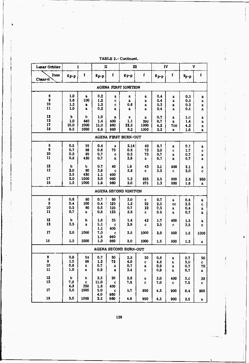
TABLE 2.- Continued.

Lunar Orbiter I n m IV V i

%. Item gp.p f gp-p £ gp-p 1 f gp-p f gp-p f Chanrelx^ 1

AGENA FIRST IGNITION |

8 1.0 a 0.2 a a a 0.4 a 0.12 a 9 1.6 100 1.2 c a a 0.4 a 0.9 a

10 1.3 a 1.2 c 0.6 a 0.3 a 0.3 a 11 1.0 a 0.2 a a a 0.4 a 0,4 a 1

12 b b 1.0 a a a 0.7 a 1.Ü a 13 1.0 440 1.4 400 1.1 390 0.7 a 1.4 a 17 10.0 1000 11.0 960 22.8 1000 4.2 700 4.2 a 18 9.5 1000 6.6 960 8.2 1000 2.2 a 1.6 a {

AGENA FIRST BURN-OUT

8 0.5 55 0.4 a 2.14 43 0.7 a 0.7 a 9 0.7 86 0.6 75 0.8 73 2.0 c 1.7 c

10 0.8 85 0.7 c 0.5 73 0.7 a 0.7 a 11 0.8 430 0.7 a 2.9 a 0.7 a 0.7 a

12 b b 0,7 40 1.9 43 2.1 400 2.1 a 13 2.0

2.5 80

430 3.9 1.1

c 400

2.8 c 3.5 c 3.0 c

17 2.0 1000 3.0 960 5.3 925 2.5 800 2.8 950 18 1.5 1000 1.9 I 960

i 2.0 875 1.3 800 1,6 a |

AGENA SECOND IGNITION

8 0.6 80 0.7 1 50 3.0 c 0.7 a 0,4 a 9 0.4 100 0.4 125 1.2 22 2.5 cc 2,5 c

j io 0.5 80 0.5 125 0.7 22 0.5 a 0.4 a 1 11 0.7 a 0.8 125 2.8 c 0.8 a 0.7 a

1 12 b b 1.8 35 1.4 42 1.7 400 1.5 a 13 3.5 a 5.1

1.1 c

400 2.9 c 3.5 c 3,5 c

17 2.0 1000 7.0 c 1.5 960

2.8 1000 2.0 800 1,6 1000

i 18 l.S 1000 1.0 960 2.0 1000 1.5 800 1,3 a

AGENA SECOND BURN-OUT

ft 0.9 58 0.7 50 2.8 50 0.8 a 0,7 50 9 1.5 86 1.2 72 4.0 c 4.8 a 5.0 c 10 0.9 a 0.7 a 0.7 a 0.9 a 0.7 70 11 1.0 a 0.9 a 3.4 c 0.9 a 0.7 a

12 b b 2.5 50 2.8 a 3.0 400 3.Ü 38 13 7.8

4.3 c

350 11.0 1.8

c 400

7.6 c 7.0 c 7.5 c

! 17 3.0 1000 5.0 4.0

c 960

5.7 950 4.5 900 6.4 900

I 18 3.0 1000 2.S 960 j 4.6 950 4.5 900 2.5 a

126

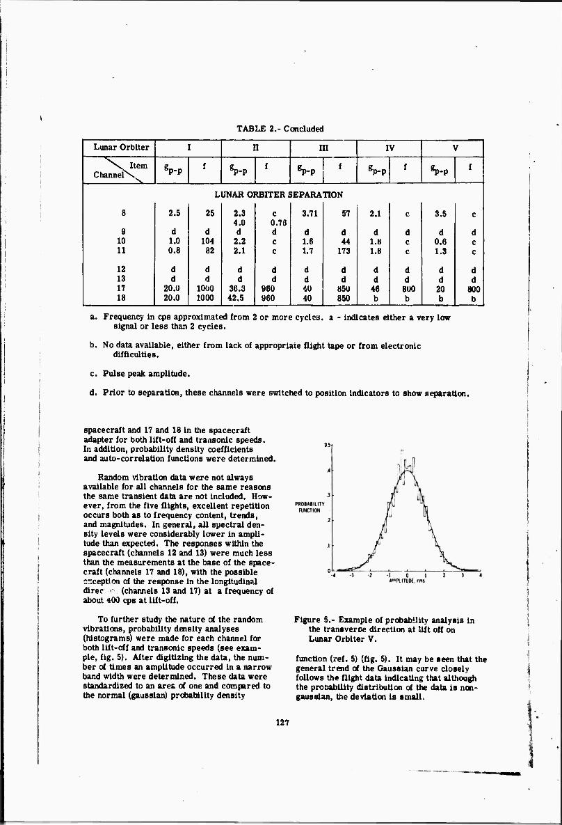
TABLE 2.- Concluded

Lunar Orbiter I n in IV V

^N. Item ChanneTV

gP-P f

Sp-P f VP f gp-p

f VP f \

LUNAR ORBITER SEPARATION

8 2.5 25 2.3 4.0

c 0.70

3.71 57 2.1 c 3.5 c

9 d d d d d d d d d d 10 1.0 104 2.2 c 1.6 44 l.U c 0.6 c 11 0.8 82 2.1 c 1.7 173 1.8 c 1.3 c

12 d d d d d d d d d d 13 d d d d d d d d d d 17 20.0 1000 36.3 960 40 851) 46 800 20 800 18 20.0 1000 42.5 960 40 850 b b b b

a. Frequency in cps approximated from 2 or more cycles, a - indicates either a very low signal or less than 2 cycles.

b. No data available, either from lack of appropriate flight tape or from electronic difficulties,

c. Pulse peak amplitude.

d. Prior to separation, these channels were switched to position indicators to show separation.

spacecraft and 17 and 18 in the spacecraft adapter for both lift-off and transonic speeds. In addition, probability density coefficients and auto-correlation functions were determined.

Random vibration data were not always available for all channels for the same reasons the same transient data are not included. How- ever, from the five flights, excellent repetition occurs both as to frequency content, trends, and magnitudes. In general, all spectral density levels were considerably lower in amplitude than expected. The responses within the spacecraft (channels 12 and 13) were much less than the measurements at the base of the spacecraft (channels 17 and 18), with the possible exception of the response in the longitudinal direr ' (channels 13 and 17) at a frequency of about 400 cps at lift-off.

To further study the nature of the random vibrations, probability density analyses (histograms) were made for each channel for both lift-off and transonic speeds (see example, fig. 5). After digitizing the data, the number of times an amplitude occurred in a narrow band width were determined. These data were standardized to an area of one and compared to the normal (gausslan) probability density

0.5 r

Figure 5.- Example of probability analysis in the transverse direction at lift off on Lunar Orbiter V.

function (ref. 5) (fig. 5). It may be seen that the general trend of the Gaussian curve closely follows the flight data indicating that although the probability distribution of the data is ncn- gaussian, the deviation is small.

127

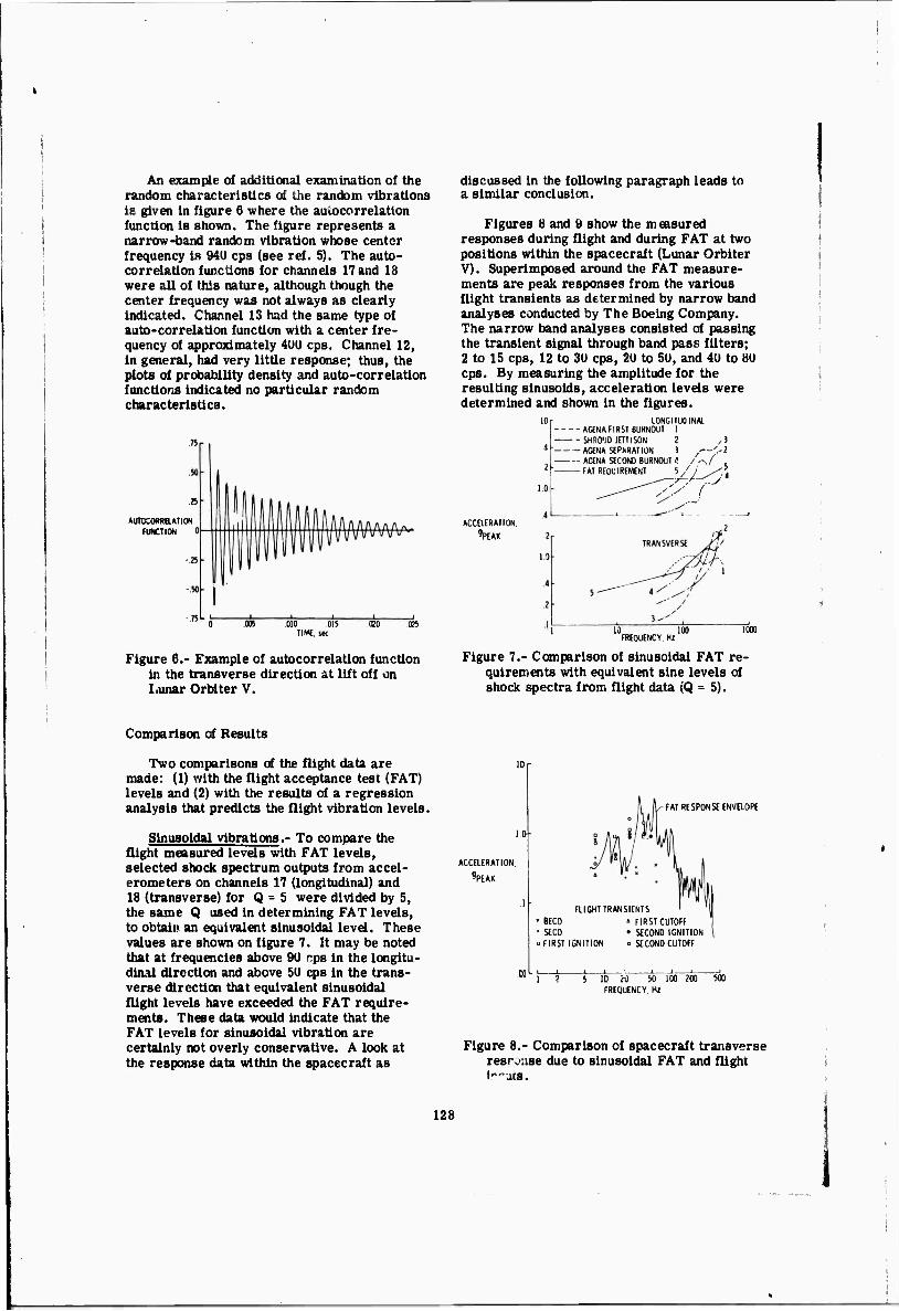
An example of additional examination of the random characteristics of the random vibrations is given in figure 6 where the autocorrelation function is shown. The figure represents a narrow-band random vibration whose center frequency Is 94ü cps (see ref. 5). The auto- correlation functions for channels 17 and 18 were all of this nature, although though the center frequency was not always as clearly indicated. Channel 13 had the same type of auto-correlation function with a center frequency of approximately 4UU cps. Channel 12, in general, had very little response; thus, the plots of probability density and auto-correlation functions indicated no particular random characteristics.

AUTCCORRaATION FUNCTION

010 015 TIMf. SK

Figure 6.- Fxample of autocorrelation function in the transverse direction at lift off on Lunar Or biter V.

discussed in the following paragraph leads to a similar conclusion.

Figures 8 and 9 show the measured responses during flight and during FAT at two positions within the spacecraft (Lunar Orbiter V). Superimposed around the FAT measurements are peak responses from the various flight transients as determined by narrow band analyses conducted by The Boeing Company. The narrow band analyses consisted of passing the transient signal through band pass filters; 2 to 15 cps, 12 to 3U cps, 2U to 5U, and 4U to BU cps. By measuring the amplitude for the resulting sinusoids, acceleration levels were determined and shown in the figures.

LONGITUDINAL --ACENA FIRST BURNOUT 1 --SHROUD JETTISON 2 /3 - — AGENA SEPARATION 3 .■—',-? - - - AGENA SECOND BURNOUT f. /\/ . - FAT REQUIREMENT i/J //,

ACCELERATION.

«PEAK

10 100 FREQUENCY. Hz

1000

Figure 7.- Comparison of sinusoidal FAT requirements with equivalent sine levels of shock spectra from flight data (Q = 5).

Comparison of Results

Two comparisons of the flight data are made: (1) with the flight acceptance test (FAT) levels and (2) with the results of a regression analysis that predicts the flight vibration levels.

Sinusoidal vibrations.- To compare the flight measured levels with FAT levels, selected shock spectrum outputs from accelerometers on channels 17 (longitudinal) and 18 (transverse) for Q = 5 were divided by 5, the same Q used in determining FAT levels, to obtain an equivalent sinusoidal level. These values are shown on figure 7. It may be noted that at frequencies above 90 cps in the longitudinal direction and above 50 cps in the transverse direction that equivalent sinusoidal flight levels have exceeded the FAT requirements. These data would indicate that the FAT levels for sinusoidal vibration are certainly not overly conservative. A look at the response data within the spacecraft as

10-

ACCELERATION,

'PEAK

01 L

FAT RESPONSE ENVaOPE

FLIGHT TRANSIENTS - BEC0 «FIRST CUTOFF • SECO • SECOND IGNITION o FIRST IGNITION o StCONO CUTOFF

5 10 iü 50 100 200 500 FREQUENCY. Hz

Figure 8.- Comparison of spacecraft transverse response due to sinusoidal FAT and flight ••"•ats.

128

1

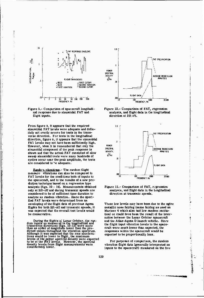
.01

i-FAT RESPONSE ENVaOPE 1.0

FUGHT TRANSIENTS

„BECO 4 FIRST CUTOFF .SECO »SECOND IGNITION "■FIRST IGNITION o SECOND CUTOFF

i 10 20 50 100 200 300 FREQUENCY, Hz

POWER SPECTRAL DENSITY,

92/Hz

.001

\FAT SPECIFICATION

AVERAGE REGRESSION ANALYSIS

100 1000 FREQUENCY.Hz

10000

Figure 9.- Comparison of spacecraft longitudinal response due to sinusoidal FAT and flight Inputs.

Figure 10.- Comparison of FAT, regression analysis, and flight data in the longitudinal direction at lift off.

From figure U, it appears that the required sinusoidal FAT levels were adequate and definitely not overly severe for tests in the transverse direction. For tests in the longitudinal direction, figure a, it appears that the sinusoidal FA1 levels may not have been sufficiently high. However, when it is remembered that only the sinusoidal component of the peak response is shown and that the actual FAT consisted of slow sweep sinusoidal tests were many hundreds of cycles occur near the peak amplitude, the tests are considered to 'ie adequate.

Rando-n vibrations.- The random flight measure vibrations can also be compared to FAT levels for the conditions both of inputs to the spacecraft, and to the results of a new prediction technique based on a regression type analysis (figs. 10 - 14). Measurements obtained only at lift-off and during transonic speeds are considered to be of sufficient time duration to analyze as random vibration. Since the specified FAT levels were determined from an enveloping of the flight data of previous Agena flights for both lift-off and transonic speeds, it was expected that the overall test levels would be conservative.

During the flights of Lunar Orbiter, the random inputs as measured in the longitudinal and transverse directions (figs. 10-13] were more than an order of magnitude lower than the predicted values throughout the vibration spectrum. Although it was expected that the rms accelerations would be lower in flight, the maximum levels of the power spectral density were expected to be at the FAT levels. However, the spectral density levels from flight measurements were considerably lower.

"I .....fAT SPECIFICATION i \

J \

POWER

SPECTRAL DENSITY,

g2/Hz


10!) 1000 FREQUENCY, Hz

10000

Figure 11.- Comparison of FAT, regression analysis, and flight data in the longitudinal direction at transonic speeds.

These low levels may have been due to the ogive metallic nose fairing (same fairing as used on Mariner 4 which also had low random excitation) or could have been the result of the interaction between the Lunar Orbiter spacecraft and the Atlas-Agena D launch vehicle. Since the flight input vibration levels to the spacecraft were much lower than expected, the responses within the spacecraft would be expected to be proportionally less.

For purposec of comparison, the random vibration flight data (generally interpreted as inputs to the spacecraft) measured on the five

129

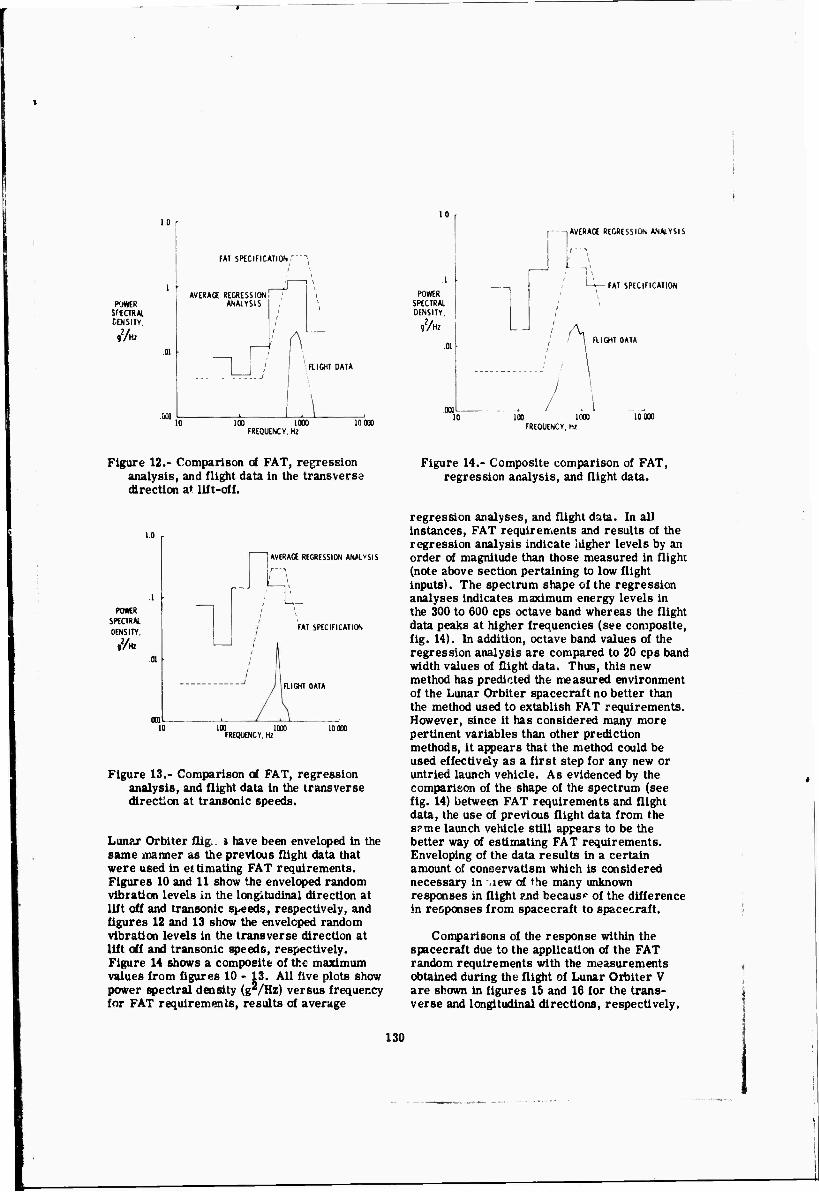
10 r

POWER SftCTRAI. TENSITY.

9%,

001

FAT SPECIFICATION '


FLIGHT DATA

loo looo FREQUENCY, Hz

10 000

10

1

POWER SPECTRAL DENSITY.

JM

f —lAVERAGE REGRESSION ANALYSIS

If-'"1

FAT SPECIFICATION

FLIGHT DATA

.. / .1 10 100 IC00 10 000

FREQUENCY. H7

Figure 12.- Comparison o* FAT, regression analysis, and flight data in the transverse direction a* lift-off.

Figure 14.- Composite comparison of FAT, regression analysis, and flight data.

1.0

POWR

SPECTRAL

DENSITY.

,7*

.001


; L- FAT SPECIFICATION

RIGHT DATA

100 1000 10000 FREQUENCY. W

Figure 13.- Comparison of FAT, regression analysis, and flight data in the transverse direction at transonic speeds.

Lunar Orbiter flig, 3 have been enveloped in the same manner as the previous flight data that were used in eiümating FAT requirements. Figures 10 and 11 show the enveloped random vibiation levels in the longitudinal direction at lift off and transonic speeds, respectively, and figures 12 and 13 show the enveloped random vibration levels in the transverse direction at lift off and transonic speeds, respectively. Figure 14 shows a composite of the maximum values from figures 10 - 13. All five plots show power spectral density (g*/Hz) versus frequency for FAT requirements, results of average

regression analyses, and flight data. In all instances, FAT requirements and results of the regression analysis indicate higher levels by an order of magnitude than those measured in flight (note above section pertaining to low flight inputs). The spectrum shape of the regression analyses indicates maximum energy levels in the 300 to 600 cps octave band whereas the flight data peaks at higher frequencies (see composite, fig. 14). In addition, octave band values of the regression analysis are compared to 20 cps band width values of flight data. Thus, this new method has predicted the measured environment of the Lunar Orbiter spacecraft no better than the method used to extablish FAT requirements. However, since it has considered many more pertinent variables than other prediction methods, it appears that the method could be used effectively as a first step for any new or untried launch vehicle. As evidenced by the comparison of the shape of the spectrum (see fig. 14) between FAT requirements and flight data, the use of previous flight data from the srme launch vehicle still appears to be the better way of estimating FAT requirements. Enveloping of the data results in a certain amount of conservatism which is considered necessary in view of the many unknown responses in flight znd because of the difference in responses from spacecraft to spacecraft.

Comparisons of the response within the spacecraft due to the application of the FAT random requirements with the measurements obtained during the flight of Lunar Orbiter V are shown in figures 15 and 16 for the transverse and longitudinal directions, respectively.

130

p»

POWER 10 SPECTRAL DENSITY,

97HZ 10

FAT RES?ONS£ ENVELOPE

Lin Off

100 1000 10000 FREQUENCY. Hi

Figure 15.- Comparison of spacecraft transverse response due to random FAT and flight inputs.

10 r

POWER 10

SPECTRAL DENSITY,

92/H2 10'4

IO-6^

FAT RESPONSE ENVELOPE

TRANSONIC LIFT OFF

10 100 1000 10000 FREQUENCY. Hz

Figure 16.- Comparison of spacecraft longitudinal response due to random FAT and flight inputs.

These data were reduced by Boeing Company. The top curves of these figures show the responses (power spectral density, PSD) due to thr- application of the maximum FAT random Inputs and the lower curves are the results of PSD

analyses of the flight data. These data indicate that the t. ends of the responses within the spacecraft in flight are the same as those that occur during FAT. Since the flight inputs were more than an order of magnitude less than FAT levels, the responses within the spacecraft were accordingly less by an order of magnitude.

CONCLUDING REMARKS

This paper has presented detailed vibration measurements from five successful Lunar Orbiter flights including peak acceleration values and predominant frequencies that occurred during the various transients, and results of power spectral density analyses during lift-oft and transonic speed conditions. It has discussed the origin of the flight acceptance test requirements and shown then to be adequate. Since the flight inputs were lower than expected, the FAT random vibration levels are considered severe. The flight data were also compared to the results of a new prediction method based on a regression analysis. For establishing vibration requirements utilizing a proven launch vehicle, the regression analysis does not provide as good a basis as does flight vibration measurements from prior flights of the launch vehicle. How- ever, the analysis may be useful in estimating vibration levels for new and untried launch vehicles.

REFERENCES

1. Houston, Allan B.: Study to Define Agena Vibration and Acoustic Environment. NASA CR-66196.

2. Mahaffey, P. R,; and Smith, K. W.: Method for Predicting Environmental Vibration Levels in Jet Powered Vehicles. Noise Control, Vol. 6, No. 4, 1960.

3. Brust, J. M.; and Himelblau, H.: Comparison of Predicted and Measured Vibration Environ- ments for Skybolt Guidance Equipment. Shock and Vibration Bulletin No. 33, Part 3, p. 231, 1964.

4. Piersol, A. G.; and Van Der Laan, W. F.: A Method for Predicting Launch Vehicle Vibration Levels in the Region of the Spacecraft Adapter. NASA CR 1227, 1968.

5. Bendat, Julius A.; and Piersol, Allan G.: Measurement and Analysis of Random Data. Published by John Wiley and Sons, Inc., New York, 1966, pp. 16 -21 and 160 - 161.

131

DISCUSSION

Mr. Bendat (Measurement Analyslfl Corp.): I think that was a very fine paper and it is very apropos to some of the remarks of the Chair- man earlier on the need »or analysis and engineering requirements to be considered together as a pair. Because there were certain analytical results available which did not quite agree with the experimental results and you had an opportun, ty to consider the reasc. s for the differences. The mathematical model which someone might use requires a great deal of care and InterpretaMc-p. There is really no sue a thing as a sine wave in nature - nothing can persist '•■ .eflnltely like a sice wave. There is no such thing as a Gaussian process in nature - I would say that any amplitude could be exceeded no matter how large It might be, so you have compromises right at the very start. If there are significant results that might be predicted you should use all the tools that are available. In some of the plots that were made in this paper, as well as the preceding paper, I did not notice complete mention of bandwidths, record lengths and other such parameters that would help one in putting some standard error on the measurements. These are the kinds at considerations that are brought to bear, together with all the engineering understanding of the problem before you get the final answers.

Mr. Delchamps (Bell Telephone Labora- tories): Have you done any distribution analysis on the peaks of the transient? You were picking a maximum and I just wondered where this was in the distribution of the peaks which you found when you did your spectrum analysis.

Mr. Clevenson: We found primarily that the distribution of peaks occurred at the natural frequencies that were shown up during the sinusoidal tests. During the flight acceptance test, various resonances occurred and the same peaks occurred during the analysis of the random tests. So we can pretty much

expect that whatever resonances are there, these frequencies are going to show up as maximum response.

Mr. Delchamps: All right for the frequencies, I was thinking about the distribution of levels. In other words, you took a level that was one of the high levels, and it was there 60 or 70 or 80 percent of the time, or maybe only 30 percent. Or maybe just a peak.

Mr. Clevenson: I very carefully specified that the table of values in the report gives the peak values of the transients as obtained from high speed oscillograms.

Mr. Delchamps: O.K. I think It would be Interesting to see the distribution of peak levels in that transient to find out whether this was an event, or two events, or a number of events in a few more events - in the same manner that you would look at the distribution of amplitudes in a random sample to find out If you have a Gaussian density function.

Mr. Clevenson: We did not do what you are asking. However, I think we could to that. We have all the various transients and we could combine them and determine an amplitude spectrum from them. I assume you mean from all of the amplitudes - all of the transients - not the amplitudes within one transient.

Mr. Delchamps: Both. When you pick the maximum, the natural question is: what else was there? That Is what I was trying to ask. Maximums, as Dr. Bendat pointed out, are at infinity, really, except that we do not measure them when they are there, unfortunately, since we are non-linear we do not see them either in the real world.

Mr. Clevenson: Maxii is is what we have measured and they are reai^ .ere.

Mr. Delchamps: I give up - you are right.

132

VIBRAnON AND ACOUSTIC ENVIRONMENT CHARACTERISTICS OF THE SATURN V LAUNCH VEHICLE

Clark J. Beck, Jr. and Donald W. The Boeing Company

CaJba

! I I

This paper presents representative examples of vibration and acoustic data from flights of the Saturn V launch vehicle and static firings of Saturn V launch vehicle stages. The purpose at the paper Is to provide vibration and acoustic environment characteristics which are pertinent to the decign of launch vehicles.

Comparisons of vibration spectra are presented which illustrate differences between flight and static firing envlrooments, effects of mass loading on the vibration environment. Vibration traosmlssioo through structure, and the effects of fluid flow rate on vibration level.

Comparisons of acoustic data are presented which indicate differences between static firing and flight acoustic environments, differences in the acoustic environment internal and external to the vehicle, and variations in sound pressure level due to engine exhaust direction.

Flight vibration and acoustic time histories are presented. The time histories are compared with time histories of (tynamic pressure and Mach number to illustrate the correlatian between these parameters and the vibration and acoustic environment.

1

!

INTRODUCTION

The Saturn V launch vehicle consists of three stages, the S-IC, S-H, and S-IVB (Figure 1). To date there have been approximately 30 static firings of the flight stages. Over 3u00 vibration measurements have been made during these static firings. In addition about 400 vibration measurements were taken during the first two flights of the Saturn V vehicle. This paper presents representative examples of vibration and acoustic data from flights of the Saturn V launch vehicle and static firings of Saturn V launch vehicle stages. The purpose of the paper is to provide vibration and acoustic environment characteristics which are pertinent to the design of launch vehicles.

STATIC FIRING AND FLIGHT VIBRATION ENVIRONMENTS

The vibration environment of a stase daring static firing and flight can differ radäcaüy «a Illus- trated in Figure 2. This flguro shows the epectnun of a typical measurement taken during S-IVB static firing as compared with a spectrum of the same measurement during the liftoff period of the Saturn V. Note the large level difference between 10 aad 500 hertz. This difference is attributed to the structure response to dissimilar acoustic noise fields produced by the engines of the stage and the launch vehicle. The S-IVB has one engine producing over 200,000 pounds thrust while the S-IC has five engines producing over 7.5 million pounds of thrust.

I.

133

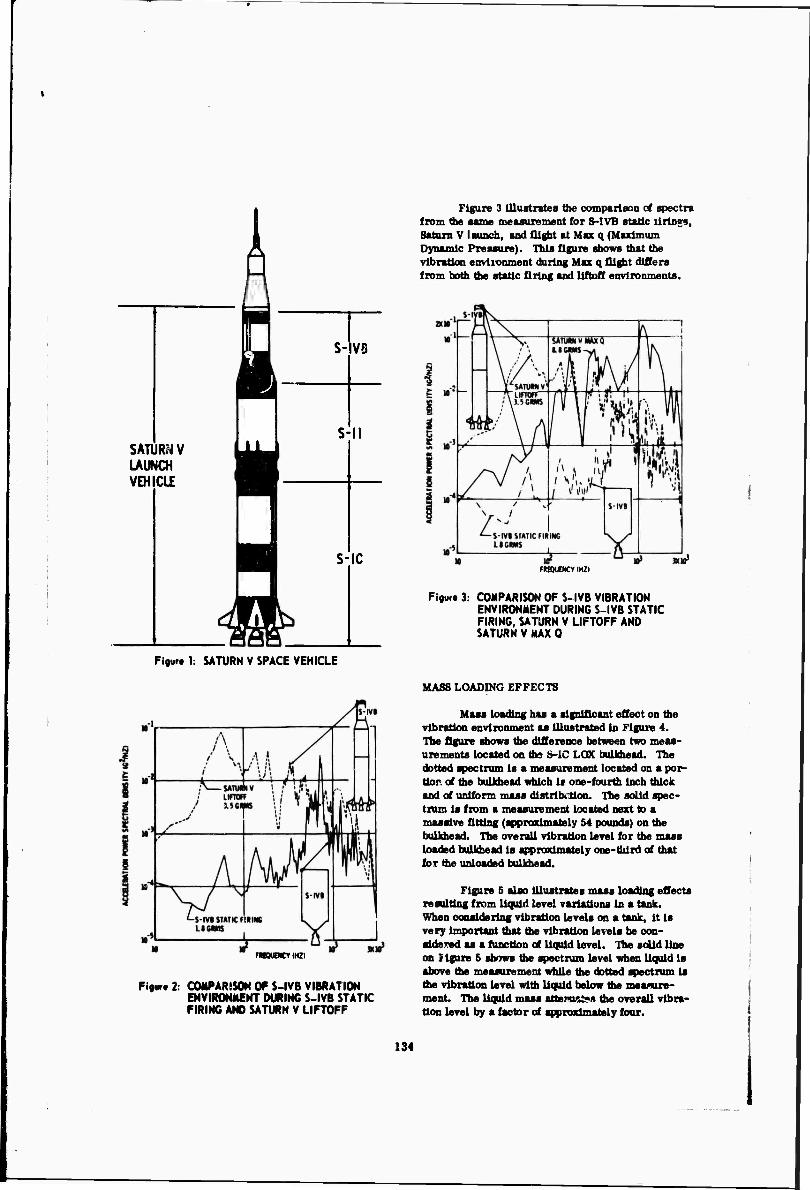
SATURN V LAUNCH

VB

S-ll

VEH CLE

S-IC

Figure 3 Illustrates tbe comparison of spectra from the same measurement for S-l VB static tlrlovs, Satan V launch, and flight at Max q (Maximum Dynamic Pressure). This figure shows that Urn vibration environment during Max q flight differs from both the static firing and liftoff envinnments.

1? FMSQUNCYIMZI

Figur* 3: COMPARISON OF S-IVB VIBRATION ENVIRONMENT DURING S-IVB STATIC FIRING, SATURN V LIFTOFF AND SATURN V MAX Q

Figure 1: SATURN V SPACE VEHICLE

mOUDKYIHZI

Fi|urt 2: COMPARSSON OF S-IVB VIBRATION ENVIRONMENT DURING S-IVB STATIC FIRING AND SATURN V LIFTOFF

MASS LOADING EFFECTS

Mass loading has a significant effect on the vibration environment as Illustrated in Figure 4. The figure shows the difference between two measurements located on ths S-IC LGK bulkhead. The dotted spectrum is a measurement located on a por- Uop of the bulkhead which le one-fourth inch thick and of uniform mass distribirfion. The solid spec- tram is from a measurement located next to a massive fitting (approximately 54 pounds) on the bulkhead. The overall vibration level for the mus loaded bulkhead is approximately one-third of that for the unloaded bulkhead.

Figure 5 also Illustrate« mass loading effects resulting from liquid level varlattona In a tank. When considering vibration levels on a tank. It is very Important that the vibration levels be considered as a function of liquid level. Hie solid line on figure 5 shows the spectrum level when liquid Is above the measurement while the dotted spectrum is the vibration level with liquid below the measurement. The liquid mass attenu^s the overall vibration level by a factor of approximately four.

134

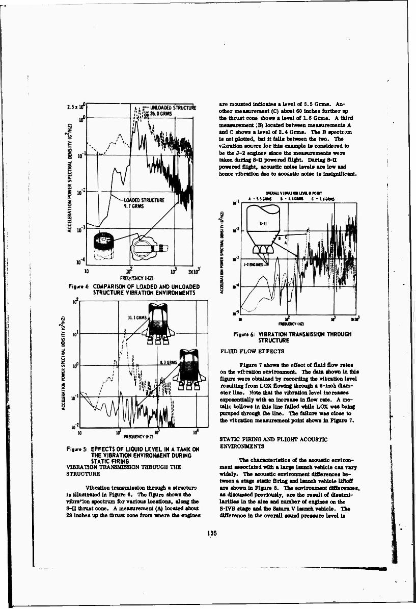
102

FRRltNCY (HZI

Figur* 4: COMPARISON OF LOADED AND UNLOADED STRUCTURE VIBRATION ENVIRONMENTS

I02

i i—

FREQUENCY ml,

Figur» 5: EFFECTS OF LIQUID LEVEL IN A TANK ON THE VIBRATION ENVIRONMENT DURING STATIC FIRING

VIBRATION TRANSMISSION THROUGH THE STRUCTURE

Vibration transmlBSloii through » structuro is UluBtnted In Figure 6. The figure show» the vlbnMon apectrum for various locationa, along the S-U tfanut cone. A meaaurement (A) located about 28 Inches up the thrust cone from where the englnae

are mounted Indicates a level of 5.5 Grma. An- other measurement (C) about 60 Inches further up the thrust cone ibowa a level of 1.6 Cms. A third measurement (B) located between measurements A and C shows a level of 2.4 Grma. The B spectrum Is not plotted, but It falls between the two. The Vibration source for this example Is considered to be the J-2 engines since the measurements wwre taken (hiring 8-n powered flight. During S-D powered flight, acoustic noise levels are low and hence vibration doe to acoestic noise la insignificant.

(MUU VIMMTHN lim • raiNT *->.5MMS I • t.4C«S C - LtCMS

Figur« 6: VIBRATION TRANSMISSION THROUGH STRUCTURE

FLUID FLOW EFFECTS

Figure 7 shows the effect of fluid flow rates on the vibration environment. The data ahown in this figure were obtained by recording the vibration level resulting from LOX flowing through a 6-lnch diameter line. Note that the vibration level increases exponentially with an increase in flow rate. A me- talic bellows In this line failed while LOK was being pumped through the line. The failure was close to the vibration measurement point shown In Figur« 7.

STATIC FIRING AND FLIGHT ACOUSTIC ENVIRONMENTS

The characteristics of the acoustic environment associated with a large launch vehicle can vary widely. The acoustic environment differences between a stage static firing and launch vehicle liftoff are shown in Figare 8. The environment differences, as discussed previously, an the result of dlssimi- larlttes In the size and number ot engines on the 8-rvB stage and the Saturn V launch vehicle. The difference in the overall sound pressure level is

135

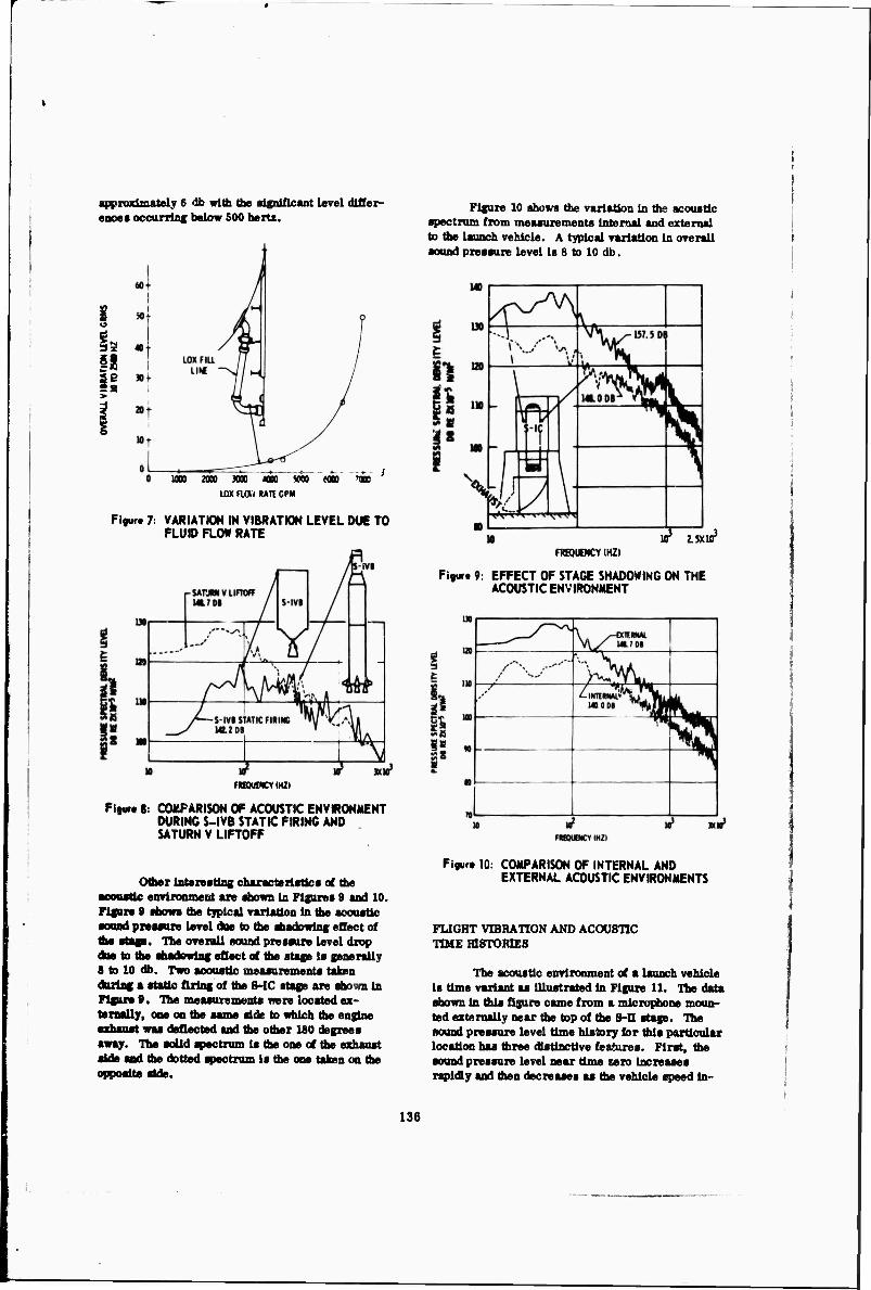
approximately 6 db with the significant level difler- eocea occurring below 500 hertz.

i s

is n

I

UDO 2900 3000 MOO WOO NOD '000 LOX aav RAIt GPM

Figure 7: VARIATION IN VIBRATION LEVEL DUE TO FLUID FLOW RATE

niBXSNCYmZ)

Figure 8: COMPARISON OF ACOUSTIC ENVIRONMENT DURING S-IVB STATIC FIRING AND SATURN V LIFTOFF

Figure 10 shows the variation In the acoustic spectnm from measurements Internal and external to the launch vehicle. A typical variation In overall sound pressure level Is 8 to 10 db.

V? 2.5X103

FKBOUCNCY (HZ)

Figure 9. EFFECT OF STAGE SHADOWING ON THE ACOUSTIC ENVIRONMENT

Other interesting characteristics of the aooustlc environment an shown In Figures 9 and 10. Ficon 9 shows (he typical variation In the acoustic sound pnssun level doe to the shadowing effect of the stags. The overall nouod pnssun level drop Ate to the shadowing effect of the stage is generally 8 to 10 db. Two acoustic meaaonments taken dozliig a static firing of the S-IC stage on shown In Flgun 9. UM measunments wen located externally, one on the same side to which the engine exhsust was deflected and the other 180 degrees away. The solid spectrum Is the one of the exhaust side and the dotted spectrum Is the one taken on the opposite aide.

Figure 10: COMPARISON OF INTERNAL AND EXTERNAL ACOUSTIC ENVIRONMENTS

FLIGHT VIBRATION AND ACOUSTIC TIME HISTORIES

The acoustic environment of a launch vehicle is time variant as illustrated in Figure 11. The data shown In this figure came from a microphone mounted externally near the top of the 8-n stage. The sound pnssun level time history for this particular location has three distinctive features. First, the sound pnssun level near time nio Incnaaes rapidly and then decnaaes u the vehicle speed In-

136

creMea. Thla is chAncterlatic of the liftoff environment. Second, the sound pleasure level Increases and decreases at a rate coincident with the variation in dynamic pressure. Third, the sound pressure level increases rather abruptly at the critical Mach Number (MCR s 0.8). Thla Increase is attributed to the presence of a normal shock wave near the microphone location. Figure 12 shows data from a vibration transducer at a location similar to the microphone location. The vibration environment has the same distinctive feature a as the acoustic environment with one exception. Ute structure responds more readily to the liftoff acoustic environment than to the flight acoustic environment.

a i

i ■ ir

• -■ ■ ■ III > • /\ -mm

„AtAi4t __t\_(m^äi. p 1*4^1 r 1

Figur« 11: CORRELATION BETWEEN ACOUSTIC ENVIRONMENT AND AERODYNAMIC PARAMETERS

WMtTMiKODNHI

Figure 12: CORRELATION BETWEEN VIBRATION ENVIRONMENT AND AERODYNAMIC CHARACTERISTICS

CONCLUSIONS

Into how th? environmental characteristics an in- fluenced by operating conditions. Ute reader should realize that the data presented represents a small sample of the available date. However, the examples discussed are characteristic of the larger body of date. These characteristics should be considered in the design of launch vehicles and equipment. An extensive blhllography has been Included with tills paper to provide a list of documents which contain a majority of the Saturn V date.

AC KNOWL EDGEME NTS

The date described in this paper were generated under National Aeronautics and Space Adminis- tration contracts.

BIBLIOGRAPHY

Saturn V Statistical AnalyiU tor Vibration and Acoustic Envltonment-Stettc Flrinc October 2, 1967; D5-15568-1; Revision A; The Boeing Company.

Saturn V Statistical AnalwU tor Vibration and Acoustic Eevlronment-Statlc Flrinc February 26, 1968; 05-15569-2; The Boeing Company.

Saturn V Stettsttcal AMIWU tor Vlbretton and Acoustic Environment-AS-SOl and AS-S02 FUght; September 3. 1968; D5-15569-3; The Boeing Company.

Saturn S-IC-501 Static Test Vibration and Acoustic Date; March 1967; OS-13644-1; Revision A; The Boeing Company.

Sattum S-IC-502 Static Test Vibration and Acoastic Data; February 1967; D6-13644-2; The Boeing Company

Saturn S-IC-503 Static Test Vibration and Acoustic Date; October 1967; DS-13644-3; The Boeing Company.

Satera S-IC-504 Static Test Vibration and Acoustic Date; January 1968; D5-13644-4; The Boeing Company.

The vibration and acoustic data in this paper are presented to provide an idea of the environmental levels associated with a large launch vehicle. The data are also selected to provide an Insight

Saturn 8-IC-605 Stelle Test Vibration and Acoustic Date: July 1968; D5-13644-5; The Boeing Company.

137

Satttra 8-IC-sni ni^it vtbrtton and AooBrtlc Vwtki Aagiut 1968; D5-13851-1; The Boeing Company.

StttiB V Port FllAt Vlbratton md AooMttc T>tt Dtto Report; AS-501;

February 1968; D5-15572-1; The Boeing Company.

Stum V Port Flight Vibration and Acourttc Teat Data Report. AS-502; June 1968; D5-15572-2; The Boeing Company.

DISCUSSION

Mr. Bendat (Mgjuwrgfcjggt AnalyBls Corp.): I hope you will accept my coumcnts objectively, but there are many many questions that your paper raises which are typical of other questions I have heard. There are so many open ended areas which would lead one to feel that these results are only a start and in many cases misleading. You show that the data is non- stationary in some of the later slides, and yet in the earlier slides you were doing spectral analysis as if the data had been entirely stationary. There is Just no way to reconcile those two matters. If the data is non-stationary, all your spectra; rpsults are wrong. There is no way to interpret the results properly. You are interested in variations which are dependent on time and you have removed time from consideration by the ordinary spectral analysis. Fur- thermore, as the chairman has mentioned a couple times earlier, there is nothing noted here about any amplitude properties, and frequently amplitude properties will reveal completely separate and distinct information. You have amplitude fluctuations which are also a function at time and cannot be handled in the usual way. But even when the data is stationary, which you may be able to Justify in certain specialized cases, even there, if the data is not Gaussian the amplitude information reveals further properties that are not revealed in this spectral density information. Here you have a case of lift-off and dynamic pressures and rapidly changing dynamic environments which are not stationary, and you cannot use stationary methods to describe the environment. The fact that you compare something that was done in the past incorrectly with something

that is being done incorrectly today still does not make a good comparison.

Mr. Caba: The measurements which you spoke of as being done in the past incorrectly were made on a static firing, and were quite stationary, and those that were compared to flight data were chosen during the lift-off period at a portion on the osclllograms that appeared to be stationary in the data reduction which showed data distribution which appeared to have a Gaussian distribution.

Mr. Woolam (Southwest Research Insti- tute): One problem which you touched on and passed over rather rapidly is the failure of the metal bellows used in piping. This seems to me to be a very serious problem. We have done some work at Southwest Research Insti- tute on vibration frequencies of bellows, which is exactly the same problem - they are predictable. The problem is the cryogenic temperatures. Failures are quite rapid and there is a good case for a good application of some sort of damper or damping material. Cryogenic temperatures are not favorable for most typical damping materials. It is quite a serious problem and, I think, one which should be considered at this time. You might make some comments further on the work on the failures of flexible baffles.

Mr. Caba: The baffles themselves caused the turbulence, and we applied the telescoping sleeve to cut down the turbulence and this seemed to solve our problem.

138

THE BLAST FIELD ABOUT THE MUZZLE OF GUNS

Peter S. Westine Southwest Research Institute

San Antonio, Texas

The blast wave propagated from the muzzle of a gun imparts a severe transient load to any structure or personnel in the vicinity. This paper outlines a procedure for estimating the maximum pressure field, impulse field, and entire transient pressure history emit'ed from the muzzle of a gun. Experi- mental test data from test firings from pistols, rifles, grenade launchers, howitzers, and naval guns establish the validity of this procedure for developing the blast field at any arbitrary location around the muzzle of a gun.

INTRODUCTION

As a result of detonating an explosive or of firing a projectile from a gun barrel by igniting a propellant, a pressure wave of finite amplitude is propagated into the surrounding atmo- sphere. Such a pressure wave causes a transient load to be imparted to any structure or person in the vicinity. In this paper, we restrict ourselves to predicting the entire tnuzele blast history at any location around a gun. The procedure which is developed takes full advantage of the similitude laws for scaling blast to predict the blast field about most weapons from a small number of experimental observations. The similitude law which this study uses is closely related to the scaling law of Hopkinson [l] because the same assumptions are required concerning the propagation of a blast under sea level atmospheric conditions.

Hopkinson's law of 1915 was developed for scaling the blast field about conventional explosive charges under sealevel conditions. Hopkinson scaling assumes that heat conduction and viscosity mav be neglected. In addition, gravitational effects are assumed to be minimal. This law for the propagation of a blast with only one spatial coordinate (propagation from a spherical charge) states that peak overpressure will scale as Eq. (1) and scaled impulse as Eq. (2)

M^

wl/3 = f(wl/3) (2)

where

P = peak overpressure

R = standoff distance

W = charge weight

I = total positive impulse

Because the density of most charges varies little, w'^3 is directly proportional to the diameter cf the charge, d. Therefore, another method of stating Hopkinson's law is to substitute the charge diameter for W1^3 into Eqs. (1) and (2) and note that P and lid are unique functions of standoff distance in charge diameters.

p-'(f) (3)

(4)

(1)

During World War II, a considerable research effort was directed towards selecting the most powerful explosive for shelly and bombs. This effort required the development of recording instrumentation capable of measuring free-air blast. The reduced data from these studies substantiated that Hopkinson scaling was the proper similitude law for scaling

139

the blast fields under ambient sea level conditions. Actually, Hopkinson's law is a special case of a more general law proposed by Sachs [2] to account for the effect of changes in ambient air pressure and temperature on overpressure and impulse. A review of Sachs1

scaling would show that the left-hand terms in Eqs. (3) and (4) are nondimensional if atmospheric conditions are added to the pi terms; however, this review will not discuss Sachs' contribution as altitude conditions are not included in this study.

Apparently Reynolds at Princeton and the Navy at David Taylor Model Basin were the first to apply Hopkinson scaling to determine the blast field about gun* [3,4]. Princeton applied Hopkinson scaling to obtain the peak pressure monitored by gages in a panel under a gun, while the Navy considered free-field overpressures and Impulses about naval guns. Both groups noted that if geometric similarity existed to the extent that

M

M2 rt&'di) 3

and

V1=V2

(5)

(6)

where

M - mass of »he projectile

E = energy in the propellant

^.Paundi Ptr

Fig. 1 - Pressure about guns. Navy technique

NM: < • Ion DiMwtir 01 Sun In Inch«

0 16 » « M >

Dlittnct In C»ii»rs Along Ion Ails

Fig. 2 - Impulse about guns, Navy technique

c = caliber of weapon

I = length of bore

V = velocity of the projectile

and the subscripts denote specific weapons, then the distribution curves for maximum pressure should be identical, provided the distances are measured in calibers. The Navy drew the additional conclusion that the distribution curves for imp^ide should be identical, if the impulse divided by the caliber of the gun were plotted against distance in calibers. Plots of isobars of constant pressure and isoclines of I/c were constructed from the Navy data with an

L|, 1^ abscissa of and an ordinate of for a

c c 30"/50 caliber naval gun. Figs. 1 and 2. These results correlated well with a 16"/45 caliber naval gun, since the deviation from true replica scaling, Eqs. (5) and (6), in the interior ballistics of the two weapons averages only 15%. In the past, the Navy felt that the length of the barrel could be disregarded in 'he scaling, but this observation, based on insufficient data, is incorrect as will be demonstrated later in this paper. These scaling observations made in the mid- 40's on the blast field -'^out guns are correct, provided the interior ballistic restrictions expressed by Eqs. (5) and (6) are maintained. The plots shown in Figs. 1 and 2 are Hopkinson's law, Eqs. (3) and (4) for spherical

charges, extended to the blast field about weapons by requiring dynamic and geometric

similarity to be maintained, Eqs. (5) and (6).

14C

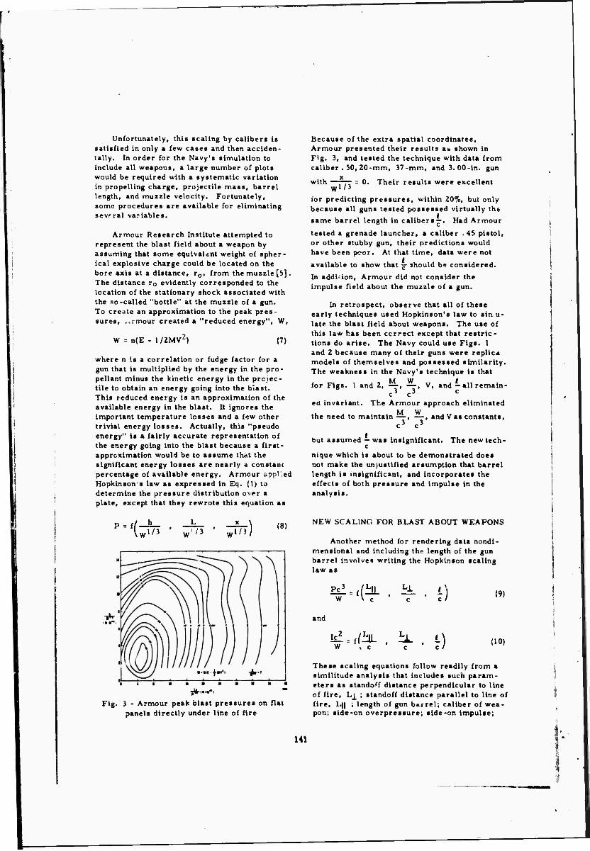
i

Unfortunately, this scaling by calibers is satisfied in only a few cases and then acciden- tally. In order for the Navy's simulation to include all weapons, a large number of plots would be required with a systematic variation in propelling charge, projectile mass, barrel length, and muzzle velocity. Fortunately, some procedure* are available for eliminating sevrral variables.

Armour Research Institute attempted to represent the blast field about a weapon by assuming that some equivaUnt weight of spherical explosive charge could be located on the bore axis at a distance, r0, from the muzzle [5]. The distance ro evidently corresponded to the location of the stationary shock associated with the so-called "bottle" at the muzzle of a gun. To create an approximation to the peak pressures, ..rmour created a "reduced energy", W,

W = n(E - 1/2MV2) (7)

where n is a correlation or fudge factor for a gun that is multiplied by the energy in the propellant minus the kinetic energy in the projectile to obtain an energy going into the blast. This reduced energy is an approximation of the available energy in the blast. It ignores the important temperature losses and a few other trivial energy losses. Actually, this "pseudo energy" is a fairly accurate representation of the energy going into the blast because a first- approximation would be to assume that the significant energy losses are nearly a constant percentage of available energy. Armour iippl'.ed Hopkinsens law as expressed in Eq. (1) to determine the pressure distribution over a plate, except that they rewrote this equation as

P = f (wl/3 W w1/3)

(8)

Fig. 3 - Armour peak blast pressures on flat panels directly under line of fire

Because of the extra spatial coordinates. Armour presented their results an shown in Fig. 3, and tested the technique with data from caliber . 50, 20-mm, 37-mm, and3.00-in. gun

with 0. Their result* were excellent wl/3

for predicting pressures, within 20%, but only because all guns tested possessed virtually the

same barrel length in caliber*—. Had Armour

tested a grenade launcher, a caliber . 45 pistol, or other stubby gun, their prediction» would have been poor. At that time, data were not

available to show that £■ should be considered.

In addition, Armour did not consider the impulse field about the muzzle of a gun.

In retrospect, observe that all of these early techniques used Hopkinson's law to sin u- late the blast field about weapons. The use of this law has been correct except that restrictions do arise. The Navy could use Fig*. 1 and 2 because many of their guns were replica model* of themselves and possessed similarity. The weakness in the Navy's technique i* that

M W I for Fig*. 1 and 2, —, —, V, and — all remain-

c3 c3 c

ed invariant. The Armour approach eliminated M W

the need to maintain —, —, and Vas constants, 3 3 c c

but assumed —was insignificant. The new tech-

nique which is about to be demonstrated doe* not make the unjuatified acaumption that barrel length is insignificant, and incorporate* the effect* of both pressure and impulse in the analysis.

NEW SCALING FOR BLAST ABOUT WEAPONS

Another method for rendering data nondl- mensional and including the length of the gun barrel involve« writing the Hopkinson scaling law as

Pc3 /Hi Ll l] W He ' T " e/

and

W 4 c i)

(9)

<10)

These scaling equations follow readily from a similitude analysis that include* such parameter* a* standoff distance perpendicular to line of fire, Lj_ ; standoff distance parallel to line of fire, Lj| ; length of gun barrel; caliber of weapon; side-on overpressure; side-on impulse;

141

I

and energy in the 'ast. Eq. (9) states that a nondimensionaiized pressure is a function ol geometric similarit ■ Eq. (iU) states that a nondimensionaiized impulse is a function of geometric similarity. [Actually, Eq. (iO)is

Ic2

not nondimensional because the pi term —- W

should be written as Ic2a

W ' where a is the

velocity of sound. Eq. (10) has been written as ^ scaling parameter with dimensions because the velocity of sound remains essentially invariant, and no need exists to include a dimensional constant, sound velocity, in the solution. ]

If the pi term —were assumed to be insig-

nificant, Eqs. (9) and (10) would represent an alternate method of presenting the Armour approach. Actually, the Armour assumption

that —is insignificant was poor and based on

too few experimental observations, as will soon be apparent. The term W in Eqs. (9) and (10) is the energy in the blast. For our purposes.

we will approximate this equation much as Armour approximated it, but no fudge factor, n, will be needed. Let Eq. (11) define the energy in the blast:

W E - 1/2MV2 (11)

All that is required to evaluate Eqs. (9) and (10) and develop the functional relationship is free- field blast data from weapon firings. Although numerous weapon firings have been conducted, the great majority of these experiments had instrumentation located behind blast shields, in the hatches of tanks, in pillboxes, or with other cbstacles interfering with the measurements of blast in a true 'ree-field. Fortunately, some testing has been conducted without introducing diffraction, refraction, and reflections. These limited data have been used to create the following observations concerning the free- field blast about guns.

FREE-FIELD BLAST PRESSURE

In Fig. 4, one observes isobars of constant nondimensional pressure on a plot with a

Fig. 4 - Isoclines of side-on pressure, Pc2l W

142

nondimensional distance from the line of fire as an ordinate and a nondimensional distance from the muzzle along the line of fire as an abscissa. This presentation for free-field blast was created after experimentally observing that the precise equation for free-field blast pressure, Eq (9)1 could be approximated

pc3 / by multiplying-rrp by —to form Eq. (12): W c

Pc2l w V (i?.)

Fig. 4 is a plot of Eq. (12), using the experimental data generated by Shapiro and Rich for a 20-mm aircraft gun [9]. Note that Fig. 4 employs Hopkinson scaling and incorporates the effects of barrel length in the solution with an empirical observation. Virtually all experimental observations before 1960 were on guns

with large barrel lengths, —. Armour and c

others concluded that the length of the barrel mattered little because these early observations were made with long-barreled weapons. Very recent test firings on a high-velocity, 40-mrr grenade launcher [8], on alow-velocity grenade launcher [6], and on caliber .45 pistol [6]. do

pc3 not correlate on a plot of .._ as a function of

W

HL —=-and —"- , as suggested by Armour scaling, c c

Only after the length of barrel has been included

in an analysis by multiplying PcJ by — can the

free-field blast pressures around all weapons be reduced to a common factor, Eq. (12).

Pc2/ Ll Fig. 5 is a plot of ——— versus for

fourteen different weapons with = 0. Notice

that excellent correlation exists and l/c varies from 8.8 up to 92.0 for the weapons plotted in Fig. 5. The grenade launchers and pistol would

Pc3

W for not correlate had wr plotted

LII —»»- = 0. The variation in weapon characteris-

c tics is much greater in Fig. 5 than the variation in weapon characteristics for earlier scaling efforts. This evaluation of the scaling for blast pressures about weapons uses data from guns firing both supersonic and subsonic pro- jectiles; the largest caliber divided by the smallest caliber is a factor of 18.5; the greatest »ncrgy divided by the least energy is a factor of Ai*' the stanioff distance covers two orders of magnttuut., «nd barrel lengths vary by more than an order nt magnitude. The correlation is

excellent especially when one considers that the data come from various sources [4, 6-9] whose authors had no thought of testing the scaling law of Eq. (12). Had muzzle velocity been measured, the rounds been hand loaded, bomb calorimeter tests been conducted on all powders, etc., a greater degree of correlation could perhaps have been obtained.

These observations on the scaling of peak pressure have required some assumptions. All the assumptions inherent in HopkU.ion scaling for peak pressures are present in this analysis. In addition to assuming a weapon under sea level ambient conditions with heat conduction, viscosity, and gravitational effects minimal, we assume that the shock is sufficiently weak so that the ratio of specific heats in air may be considered a constant. This assumption requires overpressures of 1 nder approximately 300 pal for the scaling to e rigorously correct. Inas- much as a 300-psi overpressure is extremely high, and the other assumptions associated with Hopkinson scaling are relevant, this scaling for peak overpressures seems very appropriate.

Because of a lack of information concerning the specific impetus of various propellants, a constant value was assumed for all powders,

ft-lb 350,000 lb

Of even greater consequence

was the assumption that the ratio of specific heat equaled 1.25 for all ignited propellants. The ratio of specific heat plays a prominent role because the specific energy in the propellant is calculated by dividing the specific impetus by the ratio of specific heat minus one. Undoubtedly, the lack of precise Information for calculating the energy in the blast created the greatest scatter in the experimental scaling results seen in Fig. 5. In addition, different values for available energy In the same propellant depend upon the measurement technique used to determine the energy. Virtually no reports presenting experimental blast data indicate the quantity or type of propellant. For these reasons, the propelling energy could only be estimated in developing the blast observations presented in Fig. 5.

Personal discussions with naval personnel have Indicated that a gun can emit a significant muzzle flash, especially if flash suppressors are not present in the powder. A second shock wave will be propagated if a weapon flashes. The peak overpressures associated with the second front often exceed the overpressures In the initial shock waves. Our application of Hopkinson scaling does not model these secondary explosions caused by unexpended oxygen- starved propellant igniting outside the barrel.

143

«O'ltf

z-o-icr*

1.0*10

4.0*10

Fig. 5 - Scalid side-on pressure versus scaled standoff for Army guns

Fortunately, the secondary flashing phenomena are most pronounced in large caliber «capons such as naval guns; however, some small caliber weapons will flash; Ljt, usually in the smaller caliber weapons, the second shock front is not as pronounced. Flashing is a phenomenon that can modify these experimental results.

In Fig. 6, one observes scaled free-field U ... L||

for eight different naval guns reported in Refs. [4, 10-12]. As was the case with the fourteen different Army weapons, these naval weapons appear to form a unique function. An oddity arises in that the naval guns all appear to give a lower scaled pressure than the Army weapons for a given —. The discrepancy is

c not enromous considering the art of blast measurements; nevertheless, the discrepancy is

blast pressures as a function of -J^-with —jr-=0 apparent. At -jP- = 0, Army pressures range

144

%

4.0*10

2.0» 10'*

1.0» 10''

4.0*10

Fig. 6 - Scaled side-on pressure versus standoff for naval guns

from 1, 5 times Navy pressure at —*• = 70, to

Li 2. 5 times Navy pressures at —*■ = 15. This

c phenomenon is not easily explained but may be the results of: (1) muzzle flashing which seem« more prevalent in naval guns, (2) much of the naval data being old, relative to the more recent army data with newer instrumentation giving more accurate (and higher) pressure peaks, (3) an average specific impetus for

naval powders which are usually single base propellanta and lower than the average specific impetus used in calculating data points for the double base propellanta used in Army weapons, or (4) combinations of these possible explanations. Little detailed background information is presented or. each experiment, so no more adequate explanation can be offered for lower- scaled pressures In naval guns thanArmy guns. This oddity could probably be explained had experiments been more completely reported;

145

nevertheless, with eight naval guns scaling pressures excellently as a group, and fourteen Army weapons scaling pressures excellently as another data sample, one should not discredit these experimental observations made on scaling free-field blast pressures about weapons.

FREE-FIELD SIDE-ON IMPULSE

In Fig. 7, one observes isoclines of constant scaled Impulse on a plot with a nondimen- sionalized distance from the line of fire as an ordinate and a nondiirensionalized distance from the muzzle along the line of fire as an abscissa. This presentation for scaled free-field impulse was created after experimentally observing that the precise equation for free-field impulse, Eq. (10), could be approximated by multiplying

Ic2 /I \3/4 — by (-] to form Eq. (13):

Ic5/4I3/4 /Ll Lll \ W \ c c /

Fig. 7 is a plot of Eq. (13) using the experimental data generated by Shapiro and Rich for a 20-mm aircraft gun [9]. Actually, Eq. (13)

Ic5/4|3/4 is not r ^dimensional as the pi term — w should have the velocity of sound to the first power in the expression. Eq. (13) has been written as a scaling parameter with dimensions because the velocity of sound remains invariant with no need to include a dimensional constant in the expression. Caution should be used in applying the appropriate dimensions to all impulse data. Note that Fig. 7 employs Hopkinson scaling and Incorporates the effects of barrel length in the solution through an empirical observation similar to the observation used to develop the pressure scaling.

lt»T

Ic5/V/4

Fig. 7 - Isoclines of constant scaled impulse, S

146

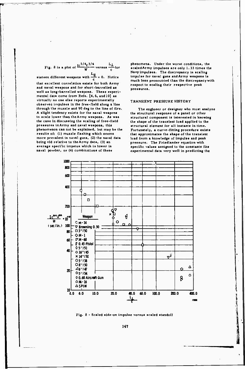
Fig. 8 is a plot of ^5/4, 3/4

W -for

ÜUo. sixteen different weapons with —'- = 0. Notice

that excellent correlation exists for both Army and naval weapons and for short-barrelled as well as long-barrelled weapons. These experimental data come from Refs. [4.6, and ID] as virtually no one else reports experimentally observed impulses in the free-field along a line through the muzzle and 90 deg to the line of fire. A slight tendency exists for the naval weapons to scale lower than the Army weapons. As was the case in discussing the scaling of free-field pressures inArmy and naval weapons, this phenomenon can not be explained, but may be the results of: (1) muzzle flashing which seems more prevalent in naval guns, (2) the naval data being old relative to the Army data, (3) an average specific impetus which is lower in naval powder, or (4) combinitions of these

phenomena. Under the worst conditions, the scaled Army impulses are only 1.33 times the Navy impulses. The discrepancy in scaling impulse for naval guns andArmy weapons is much less pronounced than the discrepancy with respect to scaling their respective peak pressure«.

TRANSIENT PRESSURE HISTORY

The engineer or designer who must analyze the structural response of a panel or other structural component is interested in knowing the shape of the transient load applied to the structural element for all instants in time. Fortunately, a curve-fitting procedure exists that approximates the shape of the transient lead from a knowledge of impulse and peak pressure. The Friedlander equation with specific values assigned to the constants fits experimental data very well in predicting the

1UUU

800

600

400 C 1

n

200

w iU

(sec/in.) 100

a n

CM Weapon

-14

X <

0 n o v Browning a 50 80 _ D3"/50

-OM-1 - (7M-60 _ ^ 0.45 Pistol

0 5"/51 - cwie

x 14"/50 " Q5"/38

O8,,/50 46"/47

60

JQ

J

20

in

0 A

05' 0 0. QM

•/54 eOAircr« -16 »IW

ft Gun 9 Ü

4.0 6.0 10,0 20.0 40.0 60.0 L.

100.0 200.0 400.0

Fig. 8 - Scaled side-on impulse versus scaled standoff

147

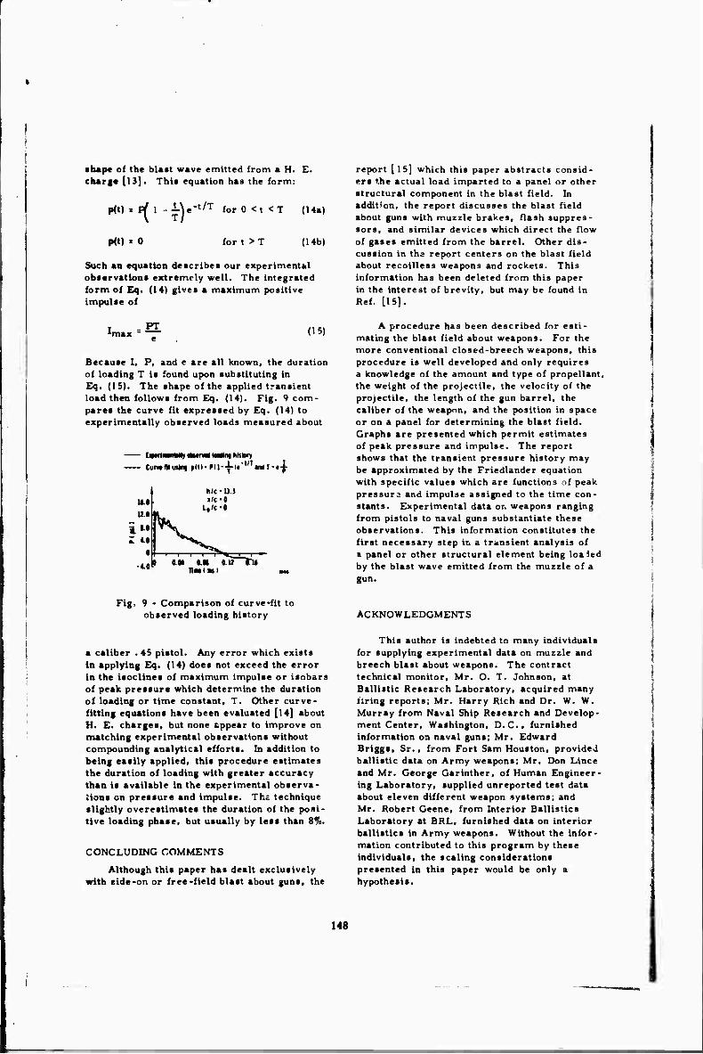
• hap« of th« blast wave emitted from a H. E. charge [13]. Thii equation has the form:

p<t) = 1^ 1 ••—\e"t/T forO<t<T (14a)

P<t) = 0 for t > T (14b)

Such an equation describe» our experimental observation* extremely well. The Integrated form of Eq. (14) gives a maximum positive impulse of

PT (15)

Because I, P, and e are all known, the duration of loading T is found upon substituting in Eq. (15). The shape of the applied transient load then follows from Eq. (14). Fig. 9 compares the curve fit expressed by Eq. (14) to experimentally observed loads measured about

faHrtaWt» mtrm Udtng hhtory CmwfHuiing »(II • Pll--^)l l/I. »T-i I

hfc-U.}

IM 12.0 !W

tlft l,(e-l

1M V £ «■( ^^

■4.0

^r**^ 0 0.0« o.« oil J"u

TlMlail

report [15] which this paper abstracts considers the actual load Imparted to a panel or other structural component in the blast field. In addition, the report discusses the blast field about guns with muzzle brakes, flash suppressors, and similar devices which direct the flow of gases emitted from the barrel. Other discussion In the report centers on the blast field about recollless weapons and rockets. This Information has been deleted from this paper In the Interest of brevity, but may be found in Ref. [15].

A procedure has been described for estimating the blast field about weapons. For the more conventional closed-breech weapons, this procedure Is well developed and only requires a knowledge of the amount and type of propellant, the weight of the projectile, the velocity of the projectile, the length of the gun barrel, the caliber of the weapon, and the position In space or on a panel for determining the blast field. Graphs are presented which permit estimates of peak pressure and impulse. The report shows that the transient pressure history may be approximated by the Friedlander equation with specific values which are functions of peak pressure and Impulse assigned to the time constants. Experimental data or. weapons ranging from pistols to naval guns substantiate these observations. This information constitutes the first necessary step In a transient analysis of a panel or other structural element being loaded by the blast wave emitted from the muzzle of a gun.

Fig. 9 - Comparison of curve-fit to observed loading history ACKNOWLEDGMENTS

a caliber . 45 pistol. Any error which exists in applying Eq. (14) does not exceed the error in the isoclines of maximum Impulse or Isobars of peak pressure which determine the duration of loading or time constant, T. Other curve- fitting equations have been evaluated [14] about H. E. charges, but none appear to improve on matching experimental observations without compounding analytical efforts. In addition to being easily applied, this procedure estimates the duration of loading with greater accuracy than is available in the experimental observations en pressure and impulse. The technique slightly overestimates the duration of the positive loading phase, but usually by less than 8%.

CONCLUDING COMMENTS

Although this paper has dealt exclusively with eide-on or free-field blast about guns, the

This author Is indebted to many Individuals for supplying experimental data on muzzle and breech blast about weapons. The contract technical monitor, Mr, O. T. Johnson, at Ballistic Research Laboratory, acquired many Uring reports; Mr. Harry Rich and Dr. W. W. Murray from Naval Ship Research and Develop- ment Center, Washington, D.C., furnished Information on naval guns; Mr. Edward Briggs, Sr., from Fort Sam Houston, provided ballistic data on Army weapons; Mr. Don Lince and Mr. George Garlnther, of Human Engineer- ing Laboratory, supplied unreported test data about eleven different weapon systems; and Mr. Robert Geene, from Interior Ballistics Laboratory at BRL, furnished data on Interior ballistics In Army weapons. Without the Infor- mation contributed to this program by these Individuals, the scaling considerations presented In this paper would be only a hypothesis.

148

r

Man/ SwRI personnel contributed by offer- ing opinion« and luggeation* for improving the observation» reported in thil paper. The author extends special recognition to Dr. W. E. Baker, project manager; Mr. P. A. Cox; and Mr. Sandor Silverman, who as authors of other aspects in the overall program on structural response of helicopters to muzzle blast, furnished many pertinent and constructive suggestions. The cooperation of these individuals and others is greatly appreciated.

REFERENCES

1. B. Hopkinson, "British Ordnance Board Minute« 13565," 1915.

2. R. G. Sachs, "The Dependence of Blast On Ambient Pressure and Impulse," Ballistic Research Labs., Rept. No. 466, Aberdeen Proving Ground, Maryland, 1944.

3. George T. Reynolds, "Muzzle Blast Pres- sure Measurements," Rept. No. PMR-21, Princeton University, April 15, 1944.

XM140 Weapons," Frankfort Arsenal, Philadelphia, Pa.. June 1967.

9. Nathan Shapiro and Harry Rich, "Measure- ment of Muzzle Blast From the 20 mm and the Short Barrel Caliber 0. 60 Aircraft Guns," NA810-059, TED-TMB-DE-201, David Taylor Model Basin, May 1949. Report C-45.

10. Preliminary Letter Report, Subject 3"/50 Gunfire Free Field Blast Measurement; preliminary report on, (a) Test Plan for Land-Based 3"/50 Caliber Gunfire Teat at NWL, Dahlgren (SMS-FS-117) of 22 May 1967, (b) ORDTASK No. 201- RDTfcE-30- 67 of 7 July 1967, From U.S. Naval Wea- pons Laboratory, Dahlgren, Va., To Naval Ordnance Systems Command, Washington, D.C., Reference WDEI: WPB: efl 8310.

11. M. F. Walther, "Gun Blast From a 5,754 Gun," N. P. G. Report No. 1608. Weapon* Development and Evaluation Laboratory, U.S. Naval Proving Ground, Dahlgren, Va., July 30, 1958.

4. U. S. Navy Gun Blast Committee, "Survey Of Research On Blast," First Interim Report, 1946, pp. 15-25

5. H. J. Barton, R. J. Heyman, and T. Schiffman, "Correlation Of Muzzle- Blast Pressures Over Flat Surfaces," Armour Research Foundation of Illinois Institute of Technology (Undated, but apparently in mid-1 950's).

6. George Garinther and Donald Lince, Unpub- lished Data, Human Engineering Labora- tory. Aberdeen Proving Ground. Maryland.

7. Ernest Stuckal. "Technical Feasibility Study and Preliminary Design Airmobility Artillery." Vol. 1, USSAVLABS Tech. Rept. 66-7, March 1966

8. Charles O. Bateman. "Blast. Flash. Gas. and Erosion Studies Ml 34, XM129, and

12. M. F. Walther, "Gun Blast From a 5"/38 Gun," N. P. C. Report No. 1307. U.S. Naval Proving Ground, Dahlgren, Va., Nov. 26, 1954.

13. C. K. Thornhill. "The Shape of a Spherical Blast Wave, " A. R. D. E. Memorandum (B) 41/59

14. N. H. Ethridge, "A Procedure for Reading and Smoothing Pressure-Time Data from H. E. and Nuclear Explosions," BRL Memorandum Report No. 1961, September 1965.

15. PeterS. Westlne, "Structural Response of Helicopters to Muzzle and Breech Blast, Volume I, Free Field Blast About Weapons," Southwest Research Institute Contract No. DAAD05-67-C-O201 with U. S. Army Ballistic Research Laboratories, Not Yet Published (Unclassified but limited distribution).

149

SPECIFICATIONS: A VIEW FROM THE MIDDLE

T. B. Delchamps Bell Telephone Laboratories, Incorporated

Whlppany, New Jersey

Specifications were the subject of extended panel discussions during the 31st and 34th Symposia. Virtually all of the traditional elements of conflict within and between the various government and Industrial agencies of supply, procurement, and use are represented In the transcripts. An effort will be made to organize this collection of viewpoints as a basis for further discussion. Since consensus In these matters lo not a reasonable expectation, the common goal of providing reliable working hardware depends upon a thorough understanding of diverse views. Justified In their own context, and upon our collective ability and willingness to apply a substantial measure of skill and Judgment In resolving differences or achieving suitable compromise.

INTRODUCTION

In lieu of moderating a panel session on shock-and-vlbratlon specifications at this symposium, the writer agreed to undertake a critical review of panel sessions on the same subject which were held during the 31st and 34th Symposia. For added Interest, the session entitled "Optimum Balance Between Component and Systems Testing" from the 31st Symposium, has been In- cluded. Representttlve comments appearing on 39 pages of text have been literally torn from context, and arrayed, with commentary. In a manner that will hopefully display them In a new and useful perspective. In general, quotation marks are reviewer's license since It Is understood that most of the material was edited for clarity prior to publication In the proceedings. Some freedom has been exercised In evaluating the panelists' Intent, but names have been withheld to protect the guilty.

WHAT IS A SPECIFICATION?

First, because the panelists didn't, let's attempt to distinguish between specifications ari standards, and then dispense with further discussion of the latter. Standards are usually bread In content and offer an

array of alternatives for doing a general class of work. Specifications, on the other hand, usually provide detailed Instructions covering how a specific Job must be done. Spe'cFTTlca- .tlons draw support from standards but tend to become autonomous in the context of a particular program. Some specifications, MIL-S-901 for example, spring full blown, like Aphrodite from the foam, without significant help from prior guiding standards. Such specifications tend to go It alone, and although their ancestry la frequently In question, their Impact on the society of things Is often dramatic, sometimes devastating, but almost always useful. In general, specifications are ambiv- alent, since they serve as the focus for both agreement and dispute. Good specifications are keystones of success -- poor specifications are wellsprings of failure. Good specifications are trustworthy, loyal, helpful, etc. — poor specifications are not.

Now let's look in on the specification panelists at the 31st and 3^th Symposia and see if we can pan some nuggets of insight from their stream of consciousness. We'll cover various general subject areas in the following order: FUNCTION, TECHNICAL BASIS,

151

FLEXIBILITY, RISK/RESPONSIBILITY/COST, and TEST CRITERIA.

FUNCTION OP SPECIFICATIONS

First, our panelists generally agreed that specifications should function tc protect both buyer and supplier at all levels of military procurement, with the focus and flexibility of requirements narrowing from systems offices in the direction of the suppliers of component parts. The transcripts confirm that the system contractor usually enjoys considerable freedom in establishing environmental design criteria and in passing his requirements down the line, with appropriate multipliers to allow for resonant buildups and as a tribute to conservatism. The component supplier, however, unless he manufactures inertial instruments, frequently re- ceives the final requirements with detached amusement and skepticism, but with no substantial concern prior to test, since he wouldn't know how to go about designing to the specification anyway. 11 ] Nevertheless, in the belief that this might be a straightforward exercise, one panelist observed that: Some problems could be traced to component manufacturers who failed to put the specification numbers into their design." 12] Perhaps this indictment reflects a degree of over-optimism regarding the quality and character of component design technology, at least where the environment is concerned.

There were valiant attempts, particularly at the 3^th Symposium, to distinguish between specifications as design criteria and as test requirements. Various types of tests which the designer must anticipate were mentioned, though not discussed in depth, and it was generally agreed that to the extent the designer can respond a priori to test criteria, he must make the effort. Usually, however, "you tr;/ to get the equipment as rugged and strong as you car under practical, yet economical conditions. If it is relatively easy to make the equipment much stronger, you do so. If it is difficult, you gc only to what you think the conditions might be."l3J It was pointed out that shipboard shock-test requirements admitted no direct design interpretation and that somehow, the designer must be given early guidance of greater sophistication than impending trial by hammer. [4] Yesterday's discussion on this subject indicates that considerable progress has been made in

this direction during the ensuing years.

TECHNICAL BASIS FOR SPECIFICATIONS

Next, what did our panelists conaider the most important single in- gredient of good specifications? Not surprisingly, nothing was said about either legal subtlety or literary excellence. The panelists views are made quite clear by such statements as: "first, one must acquire data"[5] and "the hope was that one could anticipate the vibration that the system and components would experience by analyzing or obtaining data from similar operating systems," [6] Further; "Special emphasis should be placed on the prediction of the environment." [7] And finally: "there have been rather successful attempts to predict, using models and subscale tests, what the response is going to be at the component level for future systems." [8] Needless to say, the ideal situation is one in which direct measurement of the environment at points of Interest forms the basis for design and testing specifications. Since this is clearly not possible in the early stages of many programs, we must be diligent and Imaginative in making our predictions, we must permit our specifications to respond to new information, and our first priority must be to obtain the required information by direct measurement at the earliest opportunity.

FLEXIBILITY OF SPECIFICATIONS

This brings us to one of the more difficult questions discussed by our panelists, namely: to what extent should we, can we, or must we, allow our specifications to breathe-in new information? Let's listen to the panelists: "We try to update our specifications Just as early as we possibly can."[9] "They need to be fairly constantly revised as work proceeds." (lOj "We refine (the specification) again after the first series of flights and again after a later series of flights." [11] Surprisingly, nowhere in these transcripts is there any reference made to cost impact of changes in scope-of-work midway through a program. It would seem clear, however, that responsibility rests ultimately with the originators of the top environmental spec in any given situation. This accounts for the tendency toward over-conservatism found in early equipment and component specifications, which prompts, though does not necessarily Justify such glib comments as: "To have a really good

152

specification, you shouldn't be throwing In these ignorance factors unless there Is good cause." [12] We'll all have to recognize that there almost always Is good cause, however, we must carefuTTy avoid being capricious in establishing our margins.

The possibility of simply specifying that the equipment function and survive ir the service environment, without defining that environment, was considered at some length. [13] This works fine at the system level where the prime contractor usually bears major responsibility for defining the service environments and has the experience to back It up, however, there seems to be no practical alternative to being more specific in component specifications, while main- taining some fluidity until the environments have ultimately been confirmed. At the same time we must remain sensitive to the potential penalties In cost and time associated with careless, inadequate or tardy environmental definition.

Another aspect of flexibility concerns implementation of specifications, rather than content. I refer specifically to deviations and waivers, the Scylla and Charybdis of good specsmanshlp. One panelist remarked: "We do waive certain specifications when it is Justified by the contractor." [14] From another transcript I surmised that such negotiations usually take place in a steambath: "In our debates we could all be stark naked and it would still be obvious who the contractor and who the government people were." [15J Clearly, the spectrum of waivers and deviations, both temporary and permanent, spreads from full engineering Justification, through expedlency7 to unwarranted risk. Unfortunately, timing and cost factors frequently force decisions in such matters toward the wrong end of this spectrum.

Other observations were: "His request for a change was denied by the legal people even though it was supported by reliable field data and the government technical representa- tives were in agreement." 116] And: "If thf contractor does not take exception to the spec at the time he makes the proposal, that Is his responsibility." [17J Further: "it might be worthwhile for the panel to consider the question of how much preliminary engineering It is Justi-

fiable for a company to do in order to search OLO, ahead of time, the excep- tions tney need to take to the specifications." [18] At that point, someone changed the subject. My own view is that it's not basically a question of Justification, but rather, one of contractor obligation to himself and to his customer^ we all know that it frequently costs money to discharge our obligations. If one is in the business, he ought to be required to know something about it.

A most interesting and instructive exchange Involved that favorite focus of controversy, Havy shook test requirements. Apparently, there is equipment presently at sea which has never sur- vived the rigors of MIL-S-901: "The requirement was waived when they bought the equipment --." [19] Such equipment would probably not survive the combat environment, and indeed, some has "turned out to be so bad that it required a special crew of people to keep it operating in a number 3 sea state."[20] Such waivers are presumably temporary and clearly fall In the "expedient" category. Our Navy has an Immediate Job to do, and such statements as "The fact that they are letting this equipment go to sea indicates that they admit that the specification is Inadequate" [21] seem ill-advised and unwarranted.

RISK, RESPONSIBILITY AND COST

These three elements in the specification domain are intl:.iately entwined, like the convolutions of a well-formed pretzel. Direct and In- direct reference to these three appear about 25 times In the transcripts. One panelist commented: "If you're eelllng, you want to get the best price with the least restriction. If you're buying, you want the most restrictions." [22] Sometimes it gets more complicated: "It would be necessary to establish a group of ground rules on the amount of risk you wish to take, the probability requirements for the function of this piece of equipment, and how much money you want to spend. ' [23]

Now some of my best friends are statisticians -- and while I know I can't function effectively without them, I am dismayed by the extent to which their mystique has become a substitute for engineering Judgment, rather than Its reinforcement, the role originally Intended. While it Is sometimes true that risk can be quantized within a statistical framework, in the final

153

analysis It Is sound engineering that pays off. Who Is responsible for sound engineering, statisticians or engineers? Although the answer seems obvlcjB, and even our statisticians agree, the obvious response does not appear to enjoy universal acceptance »il;hln the engineering profession, as Indicated by statements like the following: "With a proper application of probability theory, we could devise a test -- which would have associated with It a confidence level and all the other regalia that quality control requires. Within that level of confidence you could perform your design and hope that your test would simulate what you had designed Into your vehicle and equipment"[24] whatever that means.

By taking certain literary liber- ties, I have pieced together thlc dialogue: "Are contracts currently being written so that It Is the legal responsibility of the contractor to produce an Item which will perfor-ui satisfactorily In service operation?"[25] Answer: "We wrote a requirement that the total system should work In a given manner with one associate contractor becoming responsible for the system. The remaining contractors were responsible for delivering their equipment to him."[26] But unfortunately: "The systems contractor will not accept responsibility for a failure If It's not his equipment, -- (and) you can't expect each man to guarantee the performance of his single piece of equipment when he has no Idea what the associated contractors will do to his equipment after It is dellverecT" [27] At the systems level. Incentive contracting (regardless of what elüe you may aay about It) has clearly Improved this situation since 1963. One would hope that component suppliers are no longer so lacking In Information and skill that they cannot aasume some burden of responsibility. Good specifications, of course, are of fundamental Impor- tance here.

Risk, responsibility, and cost, were all implied In the following tale of one observer: "Those who knew what the problems we^e, bid high, throwing In lota of contingencies, because they could anticipate problems of shipping, handling, and so on. The lower bidder, who didn't know or care about those things, was likely to get the award. [28] Nobody popped up with an answer to this dilemma, however, the answer would seem to lie in the extent to which we allow good engineering Judgment to prevail in a cost-conscious

climate. This is seldom easy, and is often Impolitic, but with a measure of courage, and with due care in the selection of potential suppliers, in the preparation of specifications, and in the evaluation of proposals, catastroph' should be avoidable In nine out of ten cases.

TEST CRITERIA

Let's begin with an apt comment by one of the chairmen: "Test procedures and the specs which call for them are not moral questions. It is not a question of fair or unfair ^ests, but of useful teats and tests which are not useful." [29] Such tests, in the broad- est .sense, should Include those identified as either development, design qualification, (flight) acceptance, or reliability demonstration. Although the transcripts show general agreement on the Intent of tests in each of these categories, a variety of opinions erupted concerning their implementation. Both the problems and the controversy spring directly from our limited ability to predict, measure, and reproduce in the laboratory, the environments of concern. More specifically, at the very moment we are taking costly and imaginative steps toward overcoming Ignorance of the environment and refining teating techniques, we must concurrently design, build, and evaluate hardware which will perform its Intended function In the real world.

With regard to prediction: "Because of the mounting arrangements of the pump and variations of the propellant burning, it is almost im- posalble to predict the vibration spectrum and magnitude." [30] And: "Vibration specifications are based a good deal on insufficient actual measurements." [31] Finally: "There is no such thing as a predictable real environment — because they are all different, therefore the tests you devise must be a conglomerate of the real environments." [32] Regarding simulation technique: "the field vibration environment is probably omni- directional, whereas your simulation equipment is usually unidirectional."[33] And: "we are now concerned with conditions like separation nhock caused by explosive hardware which results in requirements of 5,000 g's with durations of 1/4 millisecond." [3^] I don't believe that any of us here today has yet developed a fully-satisfactory laboratory technique for handling this

154

One of the transcripts contains a brief flurry regarding the use of sine testing, Identified as a "diagnostic" tool, for deslgn-quallflcatlon purposes. It was argued (by Implication) that virtual absence of periodic components In the service environment should In- validate sine testing as a qualification requirement. [35] The man from Karshall neartlly disagreed,[36] and his position would seem fully Justified. Sine testing Is universally recognized as an essential development tool, and confirmation of Its effective prior use is clearly admlssable as a qualification requirement.

In one way or another, all of the items Just discussed contribute variability to the testing process and force us to balance our lack of testing skill and knowledge of the environment with appropriate design and testing margins. This does not absolve us, however, from recognizing the merit In the argument of one panelist: "The vibration test specification should be such that when an item of equipment passes the test that is specified it should function with reasonable certainty In the service environment. Also, a good test specification should be such that If an item of equipment functions In a service environment, we would like to think that it would pass the specified test." [37] Nevertheless, my personal view is that I would rather see a bad sppclficatlon In the latter sense, than tempt the Fates by cutting margins to the bone. Dr. Vigness put it nicely when he said: "Run It through a vibration or a shock test, find out what fails, and correct it. Do that several times and br sure that it is at least several timte ns strong as the value specified for the completed equipment. Don't worry If It's a lot stronger because sometimes this can be accomplished with only a little bit of effort." [38] Although this comment may have been made with shipboard eqi'lo- ment In mind, it has a more solid ring to me than the assurance that: "Once you have the variance, the standard deviation, and some assumed sampling distribution, it is possible to establish a test level which will, with a reasonable degree of confidence. Include all the vibration levels you've anticipated in that area of the vehicle." 13^] I guess all you have to do Is anticipate the levels and the computer will take care of the rest.

CONCLUSION

It Is the hope of any reviewer that he brings his audience a sometimes pleasing, sometimes stimulating, and sometimes downright Irritating mixture f his own and his subjects' views and

prejudices. In wading through the welter of crosscurrents evoked by the subject of shock and vibration specifications, I have not attempted to touch on all topics and attitudes represented In the transcripts, but rather, I have tried to provide a sampling of certain key viewpoints on subjects of general Interest. Perhaps I have not been entirely fair In the execution, a.»d for this I apologize. Nevertheless, If I have In any way helped to distill or clarify some of the material contributed by the panelists (while adding my own measure of bias) then I am pleased.

155

tuiPERENCES

Reference NuBber

Bulletin Number

Page Number

Reference Number

Bulletin Number

Page Number

[1] 31~II 283 [21] 34-4 157

[2] 31-11 279 [22] 31-11 291

[3] 31-11 288 [23] 31-11 301

[4] 34-4 157 [24] 31-11 296

I5] 34-4 156 [25] 31-11 292

[6] 31-11 277 [26] 31-11 292

[71 34-4 156 [27] 31-11 292

[8] 31-11 278 (28] 31-11 292

[91 34-4 159 [29] 31-11 280

[10] 34-4 153 [30] 31-11 276

[11] 31-11 290 [31] 34-4 154

[12] 34-4 156 [32] 31-11 ?98

[13] 31-11 292 [33] 31-11 296

[14] 31-11 291 [34] 34-4 155

[15] 34-4 154 [35] 34-4 161

[16] 31-11 290 [36] 34-4 161

[17] 31-11 290 [37] 34-4 156

[18] 31-11 290 [38] 31-11 288

[19] 34-4 157 t39l 34-4 l6ü

[20] 34-4 158

156 «PO •71-JJ4

THE SHOCK AND VIBRATION BULLETIM 00Bulletin 39 Part 6 (of 6 Parts) 00 00 00 THE SHOCK AND VIBRATION...

Documents

Transcript of THE SHOCK AND VIBRATION BULLETIM 00Bulletin 39 Part 6 (of 6 Parts) 00 00 00 THE SHOCK AND VIBRATION...