ENGR 220 Section 5.1-5.3. Torsional Deformation of a Circular Shaft.

RIA-80-U722 TECHNICAL
ARRADCOM LmARY
MISD USERS' MANUAL 80-5
ROBERT I. ISAKOWER
MARCH 1980
SCIENTIFIC & ENGINEERING APPLICATIONS DIVISION
MANAGEMENT INFORMATION SYSTEMS DIRECTORATE
DOVER, NEW JERSEY
DTIC QUALITY INSPBCTED 1

ARRADCOM
The MISD USERS' MANUAL 80-5
SHAFT BOOK
(DESIGN CHARTS FOR TORSIONAL PROPERTIES OF NON-CIRCULAR SHAFTS)
BY
ROBERT I. ISAKOWER
MARCH 1980
SCIENTIFIC & ENGINEERING APPLICATIONS DIVISION MANAGEMENT INFORMATION SYSTEMS DIRECTORATE
DOVER, NEW JERSEY

ACKNOWLEDGMENTS
The author would like to thank the follov/ing people for their assistance in the preparation of this report:
Mr. Robert E. Barnas, MISD, ARRADCOM, for programming the SHAFT solution.
SP4 Lillian Ishibashi, Cardiovascular Lab, Ft. Sam Houston, Texas, for preparing the input data program.
Mr. Joseph J. Sierodzinski, MISD, ARRADCOM, for the photography.
Mr Joseph DePascale's Illustrations Branch, TSD ARRADCOM and Mr. Irv Pollock (floor supervisor) for their excellent artwork.
Mrs. Sylvia Polanski, MISD, ARRADCOM for her pains- taking preparation of the report text and tables.

ABSTRACT
Design charts and tables have been developed for the elastic torsional stress analyses of free prismatic shafts, splines and spring bars with virtually all commonly encountered cross sections. Circular shafts with rect- angular and circular keyways, external splines, and milled flats along with rectangular and X-shaped torsion bars are presented. A computer program was developed at the U.S. Array ARRADCOM, Dover, N.J. site which provides a finite difference solution to the governing (POISSON's) partial differential equation which defines the stress functions for solid and hollow shafts with generalized contours. Using the stress function solution for the various shapes and Prandtl's membrane analogy, the author is able to produce dimensionless design charts (and tables) for transmitted torque and raaximum shearing stress. The design data have been normalized for a unit dimension of the cross section (radius or length) and are provided in this report for solid shapes. The eleven solid shapes presented, along with the classical circular cross section solution, provides the means for analyzing 144 combinations of hollow shafts with various outer and inner contours. Hollow shafts may be analyzed by using the computer program directly or by using the solid shape charts in this report and the orinciples of superposition based on the concept of parallel shafts. The SHAFt Torsion utility program (SHAFT) used for the generation of the data in this hand- book is a spin-off of the famous Computer Language for Your Differential Equations (CLYDE) code and employs the same basic mathematical model along with an improved algo- rithm for maximum stress. The format of the stress charts differs slightly from those of the first report in this series (Technical Report ARMID-TR-78001). Stress/torque ratio curves are presented as being more intuitively recognizable than those of stress. The source code of the SHAFT program is available upon written request and receipt of a 7-track magnetic tape.

DISCLAIMER
Thia report is issued for information and d^cuiientation pur- poses only. No representation is ivade by the Government with respect to the irfonrai n in lhi< v !■■ r' and ihe Govern- ment assumes no liability ov oblipa'ior \v; h respect thereto; nor is the material presented to be consirued as the official positif n of Ihe Depanmer.! nf she Aimy, unless so designated by other au.horized decuments.

TABLE OF CONTENTS
Page No.
The Torsion Problem 1
Design Charts and Tables ^
Accuracy of the Computerized Solution 54
Parallel Shaft Concept 55
Bibliography 64
Appendixes
A Mathematical Model Used in the CLYDE 65
Computer Program
B Extension of Model to Hollow Shafts 78
Distribution List 81

Tables
1 Element nomenclature 5
2 Split shaft, volume factor (v) 7
3 Split shaft, slope factor (dO/ds) 9
4 Single keyway shaft, volume factor (V) 11
5 Single keyway shaft, slope factor (dO/ds) 13
6 Two keyway shaft, volume factor (V) 15
7 Two keyway shaft, slope factor (d<5/ds) 17
8 Four keyway shaft, volume factor (V) 19
9 Four keyway shaft, slope factor (dO/ds) 21
10 Single square keyway with inner fillets 23
11 Single spline shaft, volume factor (V) 25
12 Single spline shaft, slope factor (dO/ds) 27
13 Two spline shaft, volume factor (V) 29
14 Two spline shaft, slope factor (dO/ds) 31
15 Four spline shaft, volume factor (V) 33
16 Four spline shaft, slope factor (dO/ds) 35
17 Square keyways and external splines, 37 volume factor (V)
18 Square keyways and external splines, 39 slope factor (dO/ds)

19 Milled shaft, volume factor (V) 41
20 Milled shaft, slope factor (dO/ds) 43
21 Rectangular shaft 45
22 Pinned shaft, volume factor (V) 47
23 Pinned shaft, slope factor (dO/ds) 49
24 Cross shaft, volume factor (V) 51
25 Cross shaft, slope factor (dO/ds) 53
Figures
1 Membrane analogy 3
2 Split shaft, torque 6
3 Split shaft, stress 8
4 Single keyway shaft, torque . 10
5 Single keyway shaft, stress 12
6 Two keyway shaft, torque 14
7 Two keyway shaft, stress 16
8 Four keyway shaft, torque 18
9 Four keyway shaft, stress 20
10 Single square keyway with inner fillets 22
11 Single spline shaft, torque 24
12 Single spline shaft, stress 26

13 Two spline shaft, torque
14 Two spline shaft, stress
15 Four spline shaft, torque
16 Four spline shaft, stress
17 Square keyways and external splines, torque
18 Square keyways and external splines, stress
19 Milled shaft, torque
20 Milled shaft, stress
21 Rectangular shaft
22 Pinned shaft, torque
23 Pinned shaft, stress
24 Cross shaft, torque
25 Cross shaft, stress
26 Parallel shaft concept
28
30
32
34
36
38
40
42
44
46
48
50
52
56
27 Milled shaft with central hole 57
28 Circular shaft with four inner splines
29 Superposition for two spline shaft
30 Superposition A for four spline shaft
31 Superposition B for four spline shaft
32 Illustrative design application 63
58
59
60
61

THE TORSION PROBLEM
The elastic stress analysis of uniformly circular shafts in torsion is a familiar and straightforward concept to design engineers. As the bar is twisted, plane sections remain plane, radii remain straight, and each section rotates about the longitudinal axis. The shear stress at any point is proportional to the distance from the center, and the stress vector lies in the plane of the circular section and is perpendicular to the radius to the point, with the maximum stress tangent to the outer face of the bar. (Another shearing stress of equal magnitude acts at the same point in the longitudinal direction.) The torsional stiffness is a function of material property, angle of twist, and the polar moment of inertia of the circular cross-section. These relationships are expressed as:
9 = T/J'G, or T = G'Q'J
and S = T-r/J, or S = C-G-r s s
where T = twisting moment or transmitted torque, C = Modulus of Rigidity of the shaft material, 0 = angle of twist per unit length of the shaft, J = polar moment of inertia of the (circular) cross-section, Ss = shear stress, and r = radius to any point.
However, if the cross-section of the bar deviates even slightly from a circle, the situation changes radically and far more complex design equations are required. Sections of the bar do not remain plane, but warp into surfaces, and radial lines through the center do not remain straight. The distribution of shear stress on the section is no longer linear, and the direction of shear stress is not normal to a radius.
The governing equation of continuity (or compatibility) from Saint-Venant's theory is
8"# + av^ " 2Ce

where O = Saint-Venant's torsion stress function. The problem then is to find a <& function which satisfies this equation and also the boundary conditions that $ = a constant along the boundary. This O function has the nature of a potential function, such as voltage, hydrodynamic velocity, or gravitational height, its absolute value is, therefore, not important; only relative values or differences are meaningful.
The solutions to this equation required complicated mathematics. Even simple, but commonplace, practical cross-sections could not be easily reduced to manageable mathematical formulae, and numerical ap- proximations or intuitive methods had to be used.
One of the most effective numerical methods to solve for Saint- Venant's torsion stress function is that of finite differences. The SHAFT computer program was applied to a number of shafts to produce the dimensionless design charts on the following pages. Most of the charts required approximately 50 computer runs for plot data generation, but once completed, the design charts for that cross-section are good for virtually all combinations of dimensions, material, and shaft twist.
The three-dimensional plot of O over the cross-section is a surface and, with O set to zero (a valid constant) along the periphery, the surface is a'domb or O membrane.1 The transmitted torque (T) is proportional to twice the volume under the membrane and the stress (Ss) is proportional to the slope of the membrane in the direction perpendicular to the mea- sured slope. Neglecting the stress concentration of sharp re-entrant corners, which are relieved with generous fillets, the maximum stress for bars with solid cross sections is at the point on the periphery nearest the center (fig. 1) .
^he best intuitive method, the membrane analogy, came from Prandtl. He showed that the compatibility equation for a twisted bar was the "same" as the equation for a membrane stretched over a hole in a flat plate, then inflated. This concept provides a simple way to visualize the to'rsional stress characteristics of shafts of any cross-section rela- tive to those of circular shafts for which an exact analytical solution is readily obtainable.

PROBLEM NODES
FINITE DIFFERENCE GRID
CROSS-SECTIONS
Figure 1. Membrane analogy.
3

DESIGN CHARTS AND TABLES
Design charts and related data which support the elastic torsional stress analyses conducted by MISD are shown in figures 2 through 25 and tables 2 through 25, respectively. The item nomenclature used in the analyses is given in table 1 .
These data are based on the stress function solution for various shapes provided by the SHAFT computer program and on Prandtl's membrane analogy.
Since the design charts are dimensionless, they can be used for shafts of any material and any dimensions.

Table 1. Element nomenclature
TORSIONAL PROPERTIES OF
SOLID, NON-CIRCULAR SHAFTS
T = TRANSMITTED TORQUE, N ■ m (lb - in.)
0 = ANGLE OF TWIST PER UNIT LENGTH, rad/mm (rad/in.
G = MODULUS OF RIGIDITY OR MODULUS OF ELASTICITY IN SHEAR, kPa (lb/in.2)
R = OUTER RADIUS OF CROSS SECTION, mm (in.)
V#—,f = VARIABLES FROM CHARTS (OR TABLES) ' ds RELATED TO VOLUME UNDER "SOAP FILM
MEMBRANE" AND SLOPE OF "MEMBRANE"
Ss = SHEAR STRESS, kPa (lb/in.2)
T
Ss
Ss T
2Ge (V)R4
GO (-^R
2-V-R3 f (■

.40
VR^O.I
.35
.30
.25
.20
.15
.10
.05
TORSIONAL STIFFNESS TRANSMITTED TORQUE,
T=2-G-e(V)Rj
J L
"•/Re
.5
Figure 2. Split shaft, torque.

Table 2. Split shaft, volume factor (V)
Y/Ri Ri/Ro
0.1 0.2 0.3 0.4 0.5 0.6
0.1 .3589 .2802 .2068 .1422 .0891 .0491
0.2 .3557 .2762 .2030 .1391 .0870 .0478
0.3 .3525 .2722 .1991 .1360 .0848 .0464
0.4 .3492 .2680 .1952 .1328 .0825 .0450
0.5 .3457 .2637 .1911 .1294 .0801 .0436
0.6 .3423 .2593 .1869 .1260 .0777 .0421
0.7 .3387 .2548 .1824 .1223 .0750 .0405
0.8 .3350 .2499 .1776 .1183 .0722 .0387
0.9 .3312 .2447 .1725 .1139 .0689 .0367
1.0 .3269 .2389 .1665 .1087 .0649 .0340

6.5
6.0
5.5
5.0
4.5
4.0
3.5
3.0
2.5
2.0
SHEAR STRESS Y/R. = 1.0
J L
0.9
0.7
0.5
0.3
0.1
J l l L 0.1 0.2 0.3 0.4 0.5 0.6
Rj/R0
Figure 3. Split shaft, stress,

Table 3. Split shaft, stress factor (f)
Y/Ri Ri/Ro
0.2 0.3 0.4 0.5 0.6
0.1 2.2140 2.2742 2.5771 3.2178 4.4650
0.2 2.2447 2.3162 2.6336 3.2977 4.5865
0.3 2.2767 2.3608 2.6942 3.3838 4.7182
0.4 2.3103 2.4082 2.7597 3.4771 4.8620
0.5 2.3461 2.4594 2.8304 3.5795 5.0233
0.6 2.3883 2.5142 2.9084 3.6930 5.2016
0.7 2.4233 2.5750 2.9955 3.8232 5.4082
0.8 2.4670 2.6423 3.0952 3.9744 5.6550
0.9 2.5142 2.7197 3.2141 4.1618 5.9691
1.0 2.5672 2.8140 3.3690 4.4218 6.4392

.80
.75
.70
.65
.60
.55 -
.50
.46
TORSIONAL STIFFNESS
TRANSMITTED TORQUE, T = 2G 0(V)R4
.40 .2 .3
B/R .4 .5
Figure 4. Single keyway shaft, torque.
10

Table 4. Single keyway shaft, volume factor (V)
B/R
0.1 0.2 0.3 0.4 0.5
0.2 .6994 .6472 .5864
0.3 .7379 .6900 .6316 .5648
0.4 .7341 .6816 .6173 .5459
0.5 .7682 .7290 .6725 .6043 .5294
0.6 .7676 .7262 .6663 .5941 .5152
0.7 .7668 .7224 .6592 .5848 .5032
0.8 .7658 .7190 .6533 .5762 .4931
0.9 .7647 .7162 .6480 .5686 .4849
1.0 .7633 .7125 .6424 .5619 .4783
1.2 .7621 .7079 .6347 .5531 .4697
1.5 .7592 .7012 .6260 .5449 .4649
2.0 .7560 .6945 .6200 .5424
11

SHEAR STRESS
MAXIMUM AT X
SS = T (f/R3)
1.20 -
1.15 -
1.10 -
1.05 -
1.00 -
Figure 5. Single keyway shaft, stress
12

Table 5. Single keyway shaft, stress factor (f)
B/R t\/ D
0.1 0.2 0.3 0.4 0.5
0.3 1.1867 1.2273 1.2538 1.2832
0.4 1.1241 1.1333 1.1642 1.2234
0.5 .9899 1.0303 1.0624 1.1155 1.1962
0.6 .9767 1.0077 1.0387 1.0960 1.1859
0.7 .9602 .9746 1.0098 1.0820 1.1848
0.8 .9393 .9466 .9953 1.0737 1.1885
0.9 .9124 .9334 .9843 1.0699 1.1944
1.0 .8773 .9131 .9749 1.0691 1.2009
1.2 .8651 .8993 .9684 1.0721 1.2120
1.5 .8300 .8829 .9655 1.0774 1.2198
2.0 .8083 .8752 .9667 1.0799
13

.80
.70
.60
.50
.40
.30
.20
TORSIONAL STIFFNESS TRANSMITTED TORQUE,
.1 .2 3 B/R
.4
Figure 6. Two keyway shaft, torque.
14

Table 6. Two key way shaft, volume factor (V)
B/R
0.1 0.2 0.3 0.4 0.5
0.2 .6187 .5226 .4195
0.3 .6927 .6008 .4944 .3831
0.4 .6853 .5848 .4688 .3517
0.5 .7524 .6753 .5678 .4457 .3246
0.6 .7511 .6698 .5562 .4277 .3014
0.7 .7496 .6625 .5429 .4112 .2818
0.8 .7477 .6558 .5319 .3962 .2655
0.9 .7454 .6505 .5221 .3829 .2522
1.0 .7426 .6433 .5117 .3713 ,2416
1 .2 .7404 .6344 .4974 .3559 ,2276
1 .5 .7346 .6215 .4813 .3416 .2197
2.0 .7283 .6086 .4703 .3373
15

1.60
1.50
1.40
1.30
1.20 -
1.10
1.00
.90
EAR STRESS
AXIMUM AT X
= T (f/R3)
0.1 0.2 0.3
B/R
0.4 0.5
Figure 7. Two keyway shaft, stress
16

Table 7. Two keyway shaft, stress factor (f)
B/R t\/ D
0.1 0.2 0.3 0.4 0.5
0.2 1.4936 1.6578 1.7501
0.3 1.2487 1.3642 1.4929 1.6491
0.4 1.1883 1.2739 1.4173 1.6313
0.5 1.0074 1.0960 1.2092 1.3882 1.6555
0.6 .9947 1.0756 1.1930 1.3902 1.7027
0.7 .9787 1.0451 1.1722 1.3981 1.7623
0.8 .9584 1.0195 1.1660 1.4127 1.8269
0.9 .9323 1.0088 1.1629 1.4318 1.8910
1.0 .8978 .9916 1.1625 1.4532 1.9502
1.2 .8864 .9827 1.1703 1.4905 2.0422
1.5 .8534 .9737 1.1855 1.5318 2.1024
2.0 .8342 .9744 1.2008 1.5463
17

.80
.70
.60
.50
V .40
.30
.20
.10
TORSIONAL STIFFNESS
TRANSMITTED TORQUE,
B/R .4
Figure 8. Four key way shaft, torque.
18

Table 8. Four keyway shaft, volume factor (V)
A/B B/R
0.1 0.2 0.3 0.4 0.5
0.2 .4806 .3361 .2114
0.3 .6088 .4511 .2965 .1705
0.4 .5952 .4253 .2624 .1384
0.5 .7214 .5769 .3983 .2333 .1140
0.6 .7190 .5672 .3805 .2119 .0962
0.7 .7161 .5541 .3605 .1935 .0842
0.8 .7124 .5422 .3444 .1783
0.9 .7080 .5330 .3304 .1662
1.0 .7024 .5203 .3160 .1572
1.2 .6982 .5051 .2974 .1482
1.5 .6870 .4832 .2787
2.0 .6748 .4622 .2692
19

2.40 -
2.20 -
2.00 -
1.80
1.60
1.40 -
1.20 -
1.00 -
0.2 0.3 B/R
Figure 9. Four keyway shaft, stress
20

Table 9. Four keyway shaft, stress factor (f)
B/R rv/ u
0.1 0.2 0.3 0.4 0.5
0.2 1.7365 2.1206 2.4931
0.3 1.3566 1.6214 2.0014 2.5784
0.4 1.3011 1.5468 1.9971 2.8271
0.5 1.0371 1.2130 1.5046 2.0591 3.1882
0.6 1.0252 1.1979 1.5115 2.1568 3.6139
0.7 1.0102 1.1737 1.5175 2.2660 4.0368
0.8 .9910 1.1541 1.5382 2.3834
0.9 .9661 1.1493 1.5609 2.4993
1.0 .9331 1.1398 1.5899 2.6030
1.2 .9232 1.1422 1.6424 2.7301
1.5 .8940 1.1511 1.7092
2.0 .8796 1.1717 1.7512
21

.75
.70
.65
.60
V
.55
.50
.45
.40
i
TRANSMITTED TORQUE
T = 2GH{\J) R4
SHEAR STRESS
.IF \
® r B
/ t \
^ B -^
J I
1.30
1.20
1.10
1.00
.90
.80
.70
0.1 0.2 0.3
B/R
0.4 0.5
Figure 10. Single square keyway with inner fillets.
22

Table 10. Single square keyway with tight inner fillets
Stress factor(f)
B/R Volume factor(V)
At keyway center(1)
At inner fillet(2)
0.1 .7703 .7804
0.2 .7206 .9715 .9777
0.3 .6504 .9941 1.0817
0.4 .5690 1.0735 1.1641
0.5 .4840 1.1977 1.2245
23

1.15 TORSIONAL STIFFNESS TRANSMITTED TORQUE,
T = 2G-0(V)R4
A/B = 2.0
1.10
1.05
1.00
Figure 11. Single spline shaft, torque.
24

A/B
0.2
0.3
0.4
0.5
0.6
0.7
0.8
0.9
1.0
1.2
1.5
2.0
Table 11. Single spline shaft, volume factor (V)
B/R ,
0.1 0.2 0.3 0.4 0.5
.7853 .7865 .7878
.7853 .7870 .7906 .7944
.7864 .7903 .7968 .8048
.7845 .7874 .7933 .8035 .8189
.7852 .7899 .7993 .8143 .8362
.7857 .7918 .8059 .8270 .8580
.7862 .7950 .8113 .8390 .8832
.7866 .7976 .8202 .8560 .9110
.7869 .7996 .8253 .8712 .9433
.7890 .8071 .8456 .9117 1.0158
.7907 .8174 .8754 .9800 1.1561
.7953 .8407 .9420 1.1404
25

0.65
0.60
0.55
0.50
0.45
0.40
■+
SHEAR STRESS
MAXIMUM AT X
SS = T (f/R3)
R
A/B
A/B = 2.0
A
J L
0.1 0.2 0.3 0.4 B/R
0.5
Figure 12. Single spline shaft, stress,
26

Table 12. Single spline shaft, stress factor (f)
B/R
0.1 0.2 0.3 0.4 0.5
0.2 .6369 .6361 .6352
0.3 .6369 .6358 .6335 .6309
0.4 .6362 .6337 .6295 .6241
0.5 .6374 .6356 .6317 .6251 .6152
0.6 .6370 .6340 .6280 .6184 .6047
0.7 .6366 .6328 .6239 .6107 .5920
0.8 .6364 .6308 .6205 .6035 .5781
0.9 .6361 .6291 .6152 .5939 .5638
1.0 .6 359 .6279 .6120 .5854 .5483
1.2 .6346 .6233 .6004 .5648 .5173
1.5 .6335 .6172 .5842 .5340 .4704
2.0 .6307 .6038 .5525 .4798 .4331
27

A/B = 2.0
isol TORSIONAL STIFFNESS TRANSMITTED TORQUE,
T = 2G 0(V)R4
1.40
1.30
1.20 -
1.10
1.00
.90
.80
.70 _L ± .1 .2 3 4
B/R
Figure 13. Two spline shaft, torque.
28

Table 13. Two spline shaft, volume factor (V)
A/B B/R
0.1 0.2 0.3 0.4 0.5
0.2 .7865 .7889 .7914
0.3 .7864 .7899 .7970 .8047
0.4 .7886 .7965 .8095 .8255
0.5 .7850 .7906 .8026 .8229 .8538
0.6 .7863 .7958 .8145 .8446 .8886
0.7 .7874 .7994 .8278 .8701 .9326
0.8 .7883 .8059 .8386 .8945 .9837
0.9 .7891 .8111 .8565 .9288 1.0400
1.0 .7897 .8152 .8668 .9595 1.1058
1.2 .7940 .8302 .9078 1.0418 1.2547
1.5 .7973 .8509 .9682 1 .1818 1.5471
2.0 .8066 .8980 1.1045 1.5172
29

0.65
0.60
0.55
0.50
0.45
0.40
0.35
SHEAR STRESS
MAXIMUM AT X
Ss= T (VR3) A/B - 0.2
4- 0.1 0.2 0.3
B/R
0.4 0.5
Figure 14. Two spline shaft, stress.
30

Table 14. Two spline shaft, stress factor (f)
A/B
0. 2
0. 3
0, 4
0. ,5
0. .6
0. .7
0, .8
0, .9
1 .0
1 .2
1 .5
2 .0
B/R
3.1 0.2 0.3 0.4 0.5
.6362 .6346 .6329
.6362 .6340 .6294 .6243
.6348 .6298 .6215 .6113
.6371 .6336 .6259 .6131 .5946
.6363 .6303 .6187 .6004 .5753
.6357 .6281 .6108 .5862 .5532
.6351 .6241 .6043 .5732 .5300
.6346 .6209 .5944 .5564 .5071
.6342 .6184 .5887 .5421 .4836
.6315 .6097 .5678 .5088 .4398
.6295 .5981 .5402 .4632 .3815
.6240 .5740 .4903 .3937
31

1.80 -
1.70 -
1.60 -
1.50 -
1.40 -
1.30 --
1.20 -
1.10 -
1.00 -
Figure 15. Four spline shaft, torque.
32

Table 15. Four spline shaft, volume factor (V)
A/B B/R
0.1 0.2 0.3 0.4 0.5
0.2 .7888 .7937 .7989
0.3 .7887 .7957 .8101 .8254
0.4 .7932 .8090 .8352 .8674
0.5 .7859 .7971 .8213 .8623 .9250
0.6 .7885 .8076 .8452 .9063 .9962
0.7 .7906 .8149 .8723 .9588 1.0877
0.8 .7924 .8280 .8944 1.0090 1.1950
0.9 .7940 .8386 .9310 1.0808 1 .3158
1.0 .7954 .8467 .9519 1.1455 1.4601
1.2 .8040 .8773 1.0378 1.3239 1.8021
1.5 .8106 .9196 1.1663 1.6438
2.0 .8292 1.0180 1.4739
33

0.65
0.60
0.55
0.50
0.45
0.40 -
4-
SHEAR STRESS
MAXIMUM AT X
Ss = T (f/R3)
A/B = 0.2
J. X 0.1 0.2 0.3 0.4 0.5
B/R
Figure 16. Four spline shaft, stress
34

Table 16. Four spline shaft, stress factor (f)
B/R A/ a
0.1 0.2 0.3 0.4 0.5
0.2 .6356 .6332 .6305
0.3 .6356 .6323 .6256 .6176
0.4 .6336 .6263 .6142 .5986
0.5 .6369 ,6318 .6206 .6019 .5756
0.6 .6358 .6273 .6106 .5848 .5510
0.7 .6349 .6240 .6001 .5670 .5257
0.8 .6341 .6187 .5913 .5516 .5028
0.9 .6334 .6144 .5794 .5344 .4842
1.0 .6328 .6109 .5720 .5199 .4714
1.2 .6293 .5998 .5508 .4989
1.5 .6265 .5860 .5279
2.0 .6192 .5630
35

(V 3 cr u o
in 0) C
a in
ra C !_ (U
■*-'
X 0)
•a c ro
>« ro
>. a;
J£ 0) !_ TO 3 cr
en
3
UL
36

Table 17. Square key ways and external splines, volume factor (V)
B/R One keyway Two keyways Four keyways
0.1 ,7633 .7426 .7024
0.2 .7125 .6433 .5203
0.3 .6424 .5117 .3160
0.4 .5619 .3713 .1572
0.5 .4783 .2416
B/R One spline
0.1 .7869
0.2 .7996
0.3 .8253
0.4 .8712
0.5 .9433
T wo splines
.7897
.8152
.8668
.9595
1 .1058
Four splines
,7954
.8467
.9519
1 .1455
1 .4601
37

2.40
2.20
2.00
1.80 f
K BYWAYS
1.60
1.40
1.20
1.00
.80
4 KEYWAYS
SHEAR STRESS
1 SPLINE
2 SPLINES
/KEYWAYS/ 4SpL|NES .,
J I I L
0.65
0.60
0.55 f
SPLINES
0.50
0.45
0.40
0.35
0.1 0.2 0.3 0.4 0.5
B/R
Figure 18. Square keyways and external splines, stress.
38

Table 18. Square keyways & enternal splines, stress factor(f)
B/R One keyway Two keyways Four keyways
0.1 .8773 .8978 .9331
0.2 .9131 .9916 1.1398
0.3 .9749 1.1625 1.5899
0.4 1.0691 1.4532 2.6030
0.5 1.2009 1.9502
B/R One spline Two splines Four splines
0.1 .6359 .6342 .6328
0.2 .6279 .6184 .6109
0.3 .6120 .5887 .5720
0.4 .5854 .5421 .5199
0.5 .5483 .4836 .4714
39

CO LU
(/) 3 LU a z oc,. u. II o^
t— —- 1- --> > rn Q —
Ml <I> _i < Z o M
ITT
=
2G
0) l- 0) z o <
a; 3
o
in
cn
40
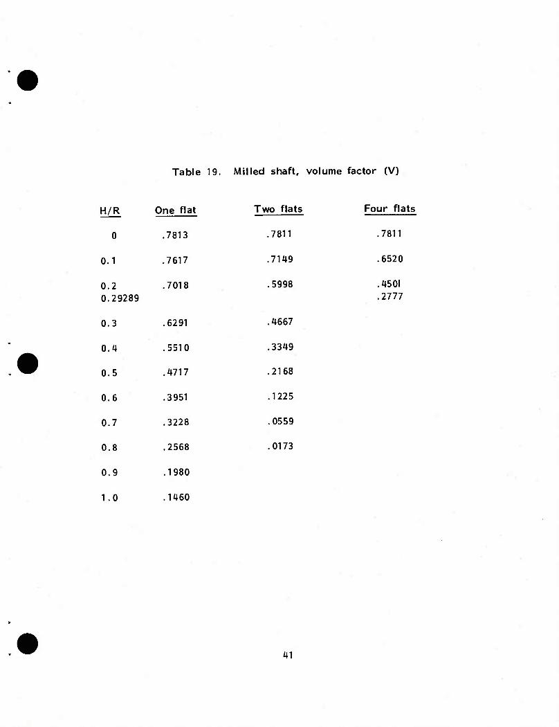
Table 19. Milled shaft, volume factor (V)
H/R One flat Two flats Four flats
0 .7813 .7811 .7811
0.1 .7617 .7149 .6520
.5998 .4501 .2777
.4667
.3349
.2168
.1225
.0559
.0173
1.0 .1460
0.2 .7018 0.29289
0.3 .6291
0.4 .5510
0.5 .4717
0.6 .3951
0.7 .3228
0.8 .2568
0.9 .1980
41

CD
d
CO
d
r^ o
co <^ o
LO LL (/) O I "0
5 « o o
0)
01 en LL o
CM
d
42

Table 20. Milled shaft, stress factor (f)
H/R One flat
0.1 .7749
0.2 .8571
0.29289
0.3 .9485
0.4 1.0593
0.5 1.1977
0.6 1.3725
0.7 1.5987
0.8 1.8975
0.9 2.3049
1.0 2.8935
Two flats
• 8199
t ,9776
1, .2045
1, .5520
2 .1237
3 .1455
5 .3129
11 .5433
Four flats
.8743
1.1848
1.7004
43

0.6 0.7 B/A
Figure 21. Rectangular shaft.
44

Table 21. Rectangular shaft
B/A
0.3
0.4
0.5
0.6
0.7
0.8
0.9
1.0
Volume factor(V)
Stress factor(f)
.05635 5.2697
.1248 3.0928
.2250 2.0587
.3559 1.4805
.5146 1.1230
.6971 .8862
.8991 .7212
1.1167 .6015
45

.8 "
.5
V
.3
TORSIONAL STIFFNESS
TRANSMITTED TORQUE,
T=2-G-e(V)R4
.1 .2
Figure 22. Pinned shaft, torque.
46

Table 22. Pinned shaft, volume factor (V)
A/R One groove
7700
Two grooves Fou r grooves
0.1 .7558 .7280
0.2 .7316 .6803 .5855
0.3 .6760 .5738 .4062
0.4 .6087 .4521 .2374
0.5 .5349 .3300 .1118
47

SHEAR STRESS
4.0
3.5
3.0
2.5
2.0
1.5
1.0
MAXIMUM AT BOTTOM OF Cl
0.1 0.2 0.3
A/R
0.4 0.5
Figure 23. Pinned shaft, stress.
48

Table 23. Pinned shaft, stress factor(f)
A/R One groove Two grooves Four grooves
0.1 1.1197 1.1374 1.1674
0.2 1.1804 1.2520 1.3800
0.3 1.2286 ^ 1.3939 1.7281
0.4 1.2894 1.6015 2.3912
0.5 1.3822 1.9211 3.8744
49

cr O
TO JZ in
U) in O
u
0)
3 CD
50

Table 24. Cross shaft, volume factor (V)
X/S Shape P Shape M
0.1 .00741 .09907
0.2 .05219 -2120
0.3 .1642 .3767
0.4 .3538 5714
0.5 .5947 .7639
0.6 .8302 -9247
0.7 1.0058 1.0368
0.8 1.0981 1.0981
51

-!>-►
SHAPE-"P" r-H X -*"
<<
t ±1 bi \y b. .X \
^
\
\ *
SHEAR STRESS
MAXIMUMS AT a & b
\ Ss = T (f/s3)
Figure 25. Cross shaft, stress
52

Table 25. Cross shaft, stress factor(f)
X/S
0.1
0.2
0.3
0.4
0.5
0.6
0.7
0.8
Shape P At a At b
26.8826 8.7805
7.2946 2.7669
3.5252 1.4172
2.1192 .9709
.7849
.6903
.6366
.6090
Shape M At a At b
4.0676 .7564
2.3702 .9225
1.5818 .8651
1.1844 .7806
.9210 .7109
.7576 .6606
.6059 .6275
.4763 .6090
53

ACCURACY OF THE COMPUTERIZED SOLUTION
To compare the SHAFT (computer) analysis of the torsion of a solid circular shaft with the exact, classical textbook solution, one quadrant of a unit-radius shaft was run with two finite-different grid spacings and the results of the equations were compared, as follows:
Equation Comparison
Torque
SHAFT
2Ge(V)R'* 2(V)RU
2(V)R^
2V
- <^
Exact
cej j
U^R" U/2)
Shear stress (max) G9(<^)R ds
(d-i) ds
GGR
1.
SHAFT Exact Deviation (%)
Torque (h=0.125 (h=0.0625)
1.5546 1.5669
1.5708 1.5708
1.03 0.25
Shear stress (h=0.125) (h=0.0625)
1.0000 1.0000
1.0 1.0
0. 0.
Area1 (h=0.125) (h=0.0625)
3.13316 3.13984
3.14159 3.14159
0.268 0.056
*Used for internal program checking.
The mathematical model used in the SHAFT computer program generation of this handbook is described in appendix A.
54

PARALLEL SHAFT CONCEPT
The torsional rigidity of a uniform circular shaft, i.e., the torque required to produce unit (one radian) displacement, is:
C = T/G = GO
In the terminology of the membrane analogy, the torsional rigidity of non-circular shafts is defined as:
c = T/e = 2-G-e(v)f(R)/e
The overall torsional rigidity of a system consisting of a number of shafts in parallel (fig. 26) is simply the sum of the torsional rigidities of the individual component shafts.
N S 1=1 I C. = Ci + C2 + Cj + ••• + c
N
N N s T.e. = es T = err, + T2 + T3 + •• + T )
1=1 1=1
The torsional rigidity of hollow shafts can be determined by re- garding the configuration as a parallel shaft arrangement. The over- all torsional rigidity can be obtained by subtracting the torsional rigidity of a shaft having the dimensions of the bore (or inner contour) from that of a shaft having the dimensions of the outer contour. The advantages of being able to apply the principles of superposition (fig. 27-31) to combinations of concentric (inner and outer) shaft con- tours are obvious. If, for example, design charts have been prepared for 20 different shaft shapes, then 400 different solutions to all possible combinations of inner and outer shaft contours (20 inner x 20 outer) are available.
55

C/) I- LL
<
C/3
<
< Q. <U u c o u
to
in
03
m CL
U3 CM
0) 1.
56

I- Q. LU
u o o in
CN CM 00
IO « Q> «■ <% O d t? CJ go d »- •- I-
m
10 I. *-• C
u
n in
-a
L
57

o Q3 -*—'
H o _ (Ji Cfc
9 & CD CO .-.^ CN in
o O DC LL q T—
'—*'
d d 00 II II Lfl
3« LL LU
> h- O qs
■ - _,- o
■ 1 O 1 O -1 "
NC
EP
T
PA
RA
L
5
00 o
11
o in CO
n
• m 0) c
•H rH
o t ■«d- CO 1'
1- 11 (0
un 00
d n
o in
ll
w (1) c c
•H
c}5 > h- M 3
D 0
c x: o +J
•H
S * "Z +J
CO m
> £
Z ^
DE
D
UT
IO
(0
CO 3 CJ
Z _i u D O , , -H
U O C^ <*>
i LU 8 • CO (N
LU h-
o 00 o 0)
3
2S r^ ^; Cn d
n "ii o > f-
ii c/) ^;
CC
58

LA 00 l>. O
n
ii >
n DC
m o -
OQ
< s oo
b II
CO II
<
II
o II
>
^■ in oo
d i
es
oo ^r
2 oo
n o
> 5!
f*—H II
in in Oi Oi in in at O) o o II
^,
cc
u> > o> in O)
in oi in at
in CM
n
in Oi in
o rv in en
o in ^ r* o) ^ in in en Oi CT) CM
■ ■ ■ o o o
o
<
< >
+J u-t
RJ X!
CO
OJ c
■H H
m
0 4J
O 4-1
c o
•H -P •H cn 0
u 0) a L0
0^ CM
a) M
cn ■H
59

in CD
in oo
l\\
en in m d
ii
>
^■ o 3 1- -~. < ^■
in QC 00
d CM (£> in
< >
CO i
CO CM
1 CM
^ o H CO aHM.,
CO ir> CM CM 00 T— ID o o *t
CO O) ^- CO o
r^-n
O) O) CT) ^ r- t— ID in in O) O) O) odd
QC
>
4-1 U-; n3
X! U3
OJ c
•H
m
M
0 U-l
M 0
c 0
•H ■p •H M O a M 0)
00
o
0 u
•H
60

IT) 00
CM IT)
00 d
n
>
CM
CO
00
d >
LT) 00
O 1 H
< E < >
00
CM d
00
CM
CO o in
o co oo CN r^ d
f^—n II ii
r^ rs r«. CO CO CO ^- ^■ f CO CO 00 o o o II
^i
cc >
+J 4-1 03
cn
0) C
•H
o
M O
M-l
03
c o
■H -p ■H m 0
a. 3
u
•H
61

ILLUSTRATIVE DESIGN APPLICATION
Find the maximum torque that may be transmitted by the
circular shaft with the interior splines (shown in Fig. 32)
if the following design criteria are to be satisfied:
1) Maximum twist 0 not to exceed 2 degrees over the full length of the shaft.
2) Maximum Shear Stress Ss not to exceed 15,000 kPa (psi)
Torque T = Z T = 5: 2G0 (V) R4 = 2G0 I (V) R
Z (V)R4 = 0.7854-(0.1058-0.0491)
= 0.7854(1" circle)-0.0567(8 tooth spline)
» 0.7287
Condition 1:
0 = 2X(TT/180)X(1/18) - 0 . 001939 (rad/in)
T = 2(12xl06) (0.001939) (0.7287) = 33,900(in-lb)
Condition 2:
(S /T = (d(t)/ds)/(2VR3) - 1.0/(2x0.7287x1 )
= 0.6862
T = S 70.6862 = 15,000/0.6862 = 21,860(in-lb) s
Use T of 21,860(in-lb) as maximum design Torque
62

0.5"r
1.0'R
V=(7r/4)R4
= (7r/4) I4 =0.7854
0.5"r
(From Table 15)
2V(R)4=2(0.8468){0.5)4
=0.1058
0.5"r
V=(7r/4)R4
=(7r/4){0.5)4
=0.0491
Figure 32. Illustrative design application,
63

BIBLIOGRAPHY
1 . F. S. Shaw, "The Torsion of Solid and Hollow Prisms in the Elastic and Plastic Range by Relaxation Methods," Australian Council for Aeronautics, Report ACA-11, November 1944.
2. F. S. Shaw, An Introduction to Relaxation Methods, Dover Publica- tions, Inc., Melbourne, Australia, 1953.
3. D. N. deG. Allen, Relaxation Methods, McGraw-Hill Book Company, Inc., New York, 1954.
4. D. H. Pletta and F. J. Maher, "The Torsional Properties of Round- Edged Flat Bars," Bulletin of the Virginia Polytechnic Institute, Vol XXXV, No. 7, Engineering Experiment Station Series No. 50, Blacksburg, Virginia, March 1942.
5. W. Ker Wilson, Practical Solution of Torsional Vibration Problems, Volume 1, 3rd Edition, John Wiley S Sons, Inc., New York, 1956.
6. R. I. Isakower and R. E. Barnas, "The Book of CLYDE - With a Torque-ing Chapter," U.S. Army ARRADCOM Users Manual MISD UM 77-3, Dover, NJ, October 1977.
7. R. I. Isakower and R. E. Barnas, "Torsional Stresses in Slotted Shafts," Machine Design, Volume 49, No. 21, Penton/IPC, Cleveland, Ohio, September 1977.
8. R.I. Isakower, "Design Charts for Torsional Properties cf Non-Circular Shafts", U.S. Army Technical Report ARMID-TR-7 8001, Dover, NJ, November 1978.
64

APPENDIX A
MATHEMATICAL MODEL USED IN THE CLYDE COMPUTER PROGRAM
As the term implies, boundary value problems are those for which conditions are known at the boundaries. These conditions may be the value of the problem variable itself (temperature, for example), the normal gradient or variable slope, or higher derivatives of the problem variable. For some problems, mixed boundary conditions may have to be specified: different conditions at different parts of the boundary. CLYDE solves those problems for which the problem variable itself is known at the boundary.
Given sets of equally spaced arguments and corresponding tables of function values, the finite difference analyst can employ forward, central, and backward difference operators. CLYDE is based upon central difference operators which approximate each differential operator in the equation.
The problem domain is overlaid with an appropriately selected grid. There are many shapes (and sizes) of overlaying Cartesian and polar coordinate grids:
rectangular square equilateral-triangular equilangular-hexagonal oblique
Throughout the area of the problem, CLYDE uses a constant-size square grid for which the percentage errors are of the order of the grid size squared (h2) . This grid (or net) consists of parallel vertical lines spaced h units apart, and parallel horizontal lines, also spaced h units apart, which blanket the problem area from left-to-right and bottom-to- top.
The intersection of the grid lines with the boundaries of the domain are called boundary nodes. The intersections of the grid lines with each other within the problem domain are called inner domain nodes. It is at these inner domain nodes that the finite difference approximations are
65

applied. The approximation of the partial differential equation with the proper finite difference operators replaces the PDE with a set of subsi- diary linear algebraic equations, one at each inner domain node. In practical applications, the method must be capable of solving problems whose boundaries may be curved. In such cases, boundary nodes are not all exactly h units away from an inner node, as is the case between adjacent inner nodes. The finite difference approximation of the harmonic operator at each inner node involves not only the variable value at that node and at the four surrounding nodes (above, below, left, and right), but also the distance between these four surrounding nodes and the inner node. At the boundaries, these distances vary unpredictably. Compensa- tion for the variation must be included in the finite difference solution. CLYDE represents the problem variable by a second-degree polynomial in two variables, and employs a generalized irregular "star" in all direc- tions for each inner node. In practice, one should avoid a grid so coarse that more than two arms of the star are irregular (or less than h units in length) . The generalized star permits, and automatically compensates for, a variation in length of any of the four arms radiating from a node. For no variation in any arm, the algorithm reduces exactly to the standard har- monic "computation stencil."
At each inner domain node, a finite difference approximation to the governing partial differential equation (PDE) is generated by CLYDE. The resulting set of linear algebraic equations is solved simultaneously by the program for the unknown problem variable (temperature, voltage, stress function, etc.) at each node in the overlaying finite difference grid. A graphics version of the program also generates, and displays on the CRT screen, iso-value contour maps for any desired values of the variable. This way, a more meaningful picture of the solution in the form of temperature distributions, constant voltage lines, stress concen- tration graphs, or even contour lines of different values of deformation and bending moment in structural problems, is made available to the engineer.
The user may also specify a finer grid spacing to increase resolu- tion in critical regions of the problem, modify the scale of the display, change the boundary of the problem or redraw it completely, and change boundary conditions and coefficients—all at the face of the screen. It is also possible to request CLYDE to pass a plane through the two dimen- sional picture displayed on the screen. This plane is perpendicular to the screen and appears as a straight line. CLYDE will generate a new display showing a cross section (or elevation) view from the edge or
66

overlaying finite difference GRID
BOUNDARY NODES value of the variable ii known at the boundary)
BOUNDARY or contour of the problem
INNER DOMAIN NODES (value of the variable to be found by finite difference solution)
Figure A-1 . Finite difference grid,
67

side. In this manner the variation or plot of the solved variable along that line is displayed on the screen. If the problem geometry is symme- trical, the designer does not have to display and work with the entire picture of the problem, he need only work with the "repeating section." In essence, the graphics user may examine the problem solution at will and redesign the problem (contour, boundary conditions, equation co- efficients, etc.) at the screen resolving the "new design" problem.
Consider the general expression:
ar)2 9^ A ok
in the r\, I, X coordinate system, where A, B, C, D are arbitrary constants.
When C = O, V 2f reduces to a two-coordinate system, in X and Y, for example:
V2f = A^ + B|^ = D Eq (2) 9x oy
Using central differences, the finite difference approximations to the partial differential operators of function f at representative node O are:
x y
X
dy2 hz y y
for a sauare arid, h = h = h and the harmonic operator Vaf becomes: -is x y
h2v 2U = [A (fi + fa) + B (fj + f4) - (A+B) 2fo ] = h2D Eq (4)
see figure A-4.
68

03
>.
o
£ c
u c n- (^ in 0) i_
■*->
o a CO
E !- 3 O C o U
i <
s_
LL
69

Figure A-3. Inner domain nodes.
7 0

K -h COMPUTATION STENCIL AT NODE 0
V2fcA4^ + B?-4r-D
Figure A-f. Harmonic operator for square star in X-Y grid,
71

This finite difference equation at node zero involves the unknown variable at node zero (f0) plus the unknown value of the variable at the four surrounding nodes (f!, f2, f3, U) > plus the grid spacing (h) . The five nodes involved form a four-arm star with node zero at the center. This algebraic (or difference) equation could be conveniently visualized as a four-arm computation stencil made up of five "balloons" connected in a four-arm star pattern and overlayed on the grid nodes. The value within each balloon is the coefficient by which the variable (f) at that node is multiplied to make up the algebraic approximation equation.
The numerical treatment of an irregular star (h^ hjii4 h3t h4) re- presents the function f near the representative node O by a second-degree polynomial in X and Y:
f(X,Y) = f0 + a^ + a2Y + a3X2 + a4Y2 + a5XY Eq (5)
Evaluating this polynomial at the neighboring nodes (1, 2, 3, 4) produces the following set of equations:
fl = f 0 +8! hj + a, h^
f 2 = fo + a2^2 + a4h22
fa = f0 - axhj + ajh,2
^4 = U -32*14 +a4h42 Eq (6)
which are then solved for a, and 84 which are necessary to satisfy the harmonic operator v2f, since:
— =a1 +2a3X + a5Y, g^l = Zaj
|^ = a2 + 2a4Y + asX, 0 = 234 Eq (7)
and
V2f = A (2a,) +B (234) Eq (8)
72

Performing the necessary algebraic operations, substituting results,
collecting terms, and using the following ratios:
bj hi h b2 - h
h, h
hs u _ h* Eq (9)
The harmonic operator becomes:
h2 V2f0 = 2A
f, +• 2B
0 = bi (bi+bj) 1 b2{b2+b4) f, +
2A f, +
2B + b3(b1+b3) 3 b4(b2+b4) 4 f. +
(J£.+ JB , = h2D b1b2 b2b4
Eq (10)
See figure A-5.
When C^O, V2f can be applied to an axisymmetric cylindrical co-
ordinate system, in Rand Z, for example:
2r A a2f 0 a2f c af n Eq (11)
For a regular star, the harmonic operator becomes (in a similar
manner to equation 4):
Ch h2V2f0= A(f1 +f3) +B(f2 +f4) +— (f2-f4)
2Rr
- (A + B)2 f0 = h'D Eq (12)
See figure A-6.
73

IRREGULAR STAR AT NODE 0 a
NEIGHBORING NODES {I. 2.3 ,4,)
bi«h /h
COMPUTATION STENCIL AT NODE 0
FOR
Figure A-5. Harmonic operator for irregular star in X-Y grid.
74

Figure A-6. Harmonic operator for square star for R-Z grid,
75

For an irregular star (hj ^ h2 ^ hj ^ 114), the harmonic operator
becomes (in a manner similar to equation 10):
■.2 2. i 2A f 2B h vfo ^MMbJ fl+b2(b2+b4)f2 +
2A f 2B f + + b3(b1+b3) 3 b4(b2+b4) 4
1 Ch ba f k Ro b2(b2+b4) 2 b4(b2+b4)
i f Z2 f +
r ] 1 2A_ ^ ^B_ _ Ch cb«-b4 j f !
bjbj b2b4 Ro b2b4 ^
= h2D Ec1 (13)
See figure A-7.
Equations 10 and 13 are employed in the programmed solutions for Cartesian and cylindrical coordinates, respectively.
76

b, shi /h
©-
©T-^
Figure A-7. Harmonic operator for irregular star in R-Z grid,
77

APPENDIX B
EXTENSION OF MODEL TO HOLLOW SHAFTS
This would appear to be a simple matter of solving the governing PDE over a multiply-connected boundary, were it not for the uncertainty concerning boundary conditions. The actual value of the problem variable at the boundary was not important in the torsion application, only the difference in the problem variable at various points mattered. The problem variable at the boundary could be assumed to have any value, as long as there was only one boundary. With two or more boundaries the solution calls for a different approach.
1 The stress function is obtained as the superposition
of two solutions, one of which is adjusted by a factor (k). This is the programmed solution to shafts with a hole. The hole may be of any shape, size, and location. The two solutions, to be combined, are shown in figure B-l: equa- tions and boundary conditions. Once the contour integrals are taken around the inner boundary of area A^, the only unknown, k, may be readily obtained. The contour integral, which need not be evaluated around the actual boundary, may be taken around any contour that encloses that boundary, and includes none other (for example, see shaded area Ag) in figure B-l.
LF.S. Shaw, The Torsion of Solid and Hollow Prisms in the Elastic and Plastic Range by Relaxation Methods, Austral- ian Council for Aeronautics, Report ACA-li, November 194 4, pp 8,11,23
78

V2^0 =-2 V2iI/,= o
-2AB=,f,|^dstk(f,|fids
Figure B-1 . Mathematical approach to hollow shaft problem,
79

80

DISTRIBUTION LIST
Commander U.S. Army Armament Research
and Development Command ATTN: DRDAR-TD
DRDAR-LCU-T, Mr . J . Dubin Mr. A. Berman Mr . J . Pearson
DRDAR-LCF-A, Mr. B. Schulman Dr. F. Tepper Mr. L. Wisse
DRDAR-LCA, Mr. L. Rosendorf Mr. C. Larson Mr. B. Knutelski
DRDAR-SCS, Mr. H. Cohen Mr. E. Jarosjewski Mr. R. Kwatnoski Mr. J . Bevelock
DRDAR-SCF, Mr. A. Tese DRDAR-MS DRDAR-MSA, Mr. R. Isakower (30)
Mr. R. Barnas Mr . J . Sierodzinski
DRDAR-MSM, Mr. B. Barnett (5) DRDAR-MST, Mr . I. Rucker DRDAR-MSH, Mr. A. C. Edwards DRDAR-TSS (5)
Dover, NJ 07801
Commander U.S. Army Armament Research
and Development Command ATTN: DRDAR-LCB, Mr . J . Pascale Watervliet, NY 12189
Commander U.S. Army Armament Research
and Development Command ATTN: DRDAR-BLB, Dr . S . Taylor
DRDAR-MSC, Mr. M.Wrublewski
Aberdeen Proving Ground, MD 21005
81

Commander U.S. Army Armament Research
and Development Command ATTN: DRDAR-MSE, Mr. S. Goldberg Aberdeen Proving Ground, MD 21010
Commander Brook Army Medical Center ATTN; SP4 Lillian Ishibashi Cardiovascular Lab Data Analysis Fort Sam Houston, TX 78234
Commander U.S. Army Missile Research
and Development Command ATTN: DRDMI-HRD, Mr. Siegfried H. Lehnigk Redstone Arsenal, AL 35809
Commander U.S. Army Research and Technology Laboratories ATTN: DAVDL-EU-TSC Fort Eustis, VA 23604
Commander U.S. Army Tank-Automotive Research
and Development Command ATTN: DRDTA-UL, Technical Library Warren, Ml 48090
Commander U.S. Navy Surface Weapons Center ATTN: NSWC, Mr. W. P. Warner
Technical Library
Dahlgren, VA 22448
Commander U.S. Navy Surface Weapons Center White Oak Laboratory ATTN: NOL, Mr. J. Franklin
Technical Library Silver Spring, MD 20910
82

Commander U.S. Naval Ship Research and
Development Center ATTN: NSRDC, Mr. P. Matula
Mr. J. McKey Technical Library
Bethesda, MD 20034
Commanding Officer NASA Langley Research Center ATTN: NLRC, Dr. Fulton
Technical Library
Hampton, VA 22065
Martin Marietta Aerospace Denver Division ATTN: Mr. Michael M. Davis Mass Properties Engineering
PO Box 179 Denver, CO 80201
Sperry Vickers North American Group ATTN: Mr. Frank Rosett 1401 Crooks Road Troy, Ml 48084
The Bendix Corporation ATTN: Mr. David F. Theilen Department 744, MC45 PO Box 1159 Kansas City, MO 64141
College of the City of New York Technology Department ATTN: Professor Sandor Halasz, Chairman
Steinman Hall 207-14 Convent Avenue and 138th Street New York, NY 10031
Professor Theodore Baumeister Yonges Island, SC 29494
83

College of the City of New York Mechanical Engineering Department ATTN: Professor Eugene A. Avallone
Convent Avenue & 138th Street New York, NY 10031
E.I. duPont deNemours and Company ATTN: Information Systems Dept,
Mr. Theodore Baumeister, III
Engineering Dept, Dr. Joseph H. Faupel (2)
Wilmington, DE 19898
University of Wisconsin ATTN: Dr. Warren C. Young (2) 537 Engineering Research Bldg 1500 Johnson Drive Madison, Wl 53706
Stanford University ATTN: Dr. W. Flugge (2) Applied Mechanical Engineering Dept Stanford, CA 94305
Defense Documentation Center (12) Cameron Station Alexandria, VA 22314
Weapon System Concept Team/CSL ATTN: DRDAR-ACW Aberdeen Proving Ground, MD 21010
Technical Library ATTN: DRDAR-CU-L Aberdeen Proving Ground, MD 21010
Technical Library ATTN: DRDAR-TSB-S Aberdeen Proving Ground, MD 21005
84

Benet Weapons Laboratory Technical Library ATTN: DRDAR-LCB-TL Watervliet, NY 12189
Commander U.S. Army Armament Materiel
Readiness Command ATTN: DRSAR-LEP-L Rock Island, IL 61299
Director U.S. Army TRADOC Systems
Analysis Activity ATTN: ATAA-SL (Tech Library) White Sands Missile Range, NM 88002
U.S. Army Materiel Systems Analysis Activity
ATTN: DRXSY-MP Aberdeen Proving Ground, MD 21005
Syracuse University Department of Mechanical & Aerospace Engineering
ATTN: Professor Charles Libove 139 E.A. Link Hall Syracuse, N.Y. 13210
85

UNCLASSIFIED SECURITY CLASSIFICATION OF THIS PAGE (When Data Entered)
REPORT DOCUMENTATION PAGE 1. REPORT NUMBER
MISD USERS MANUAL 2. GOVT ACCESSION NO
UM 8Q-5 4. TITLE rand Subm/e^THE SHAFT BOOK
(DESIGN CHARTS FOR TORSIONAL PROPERTIES OF NON-CIRCULAR SHAFTS)
READ INSTRUCTIONS BEFORE COMPLETING FORM
3. RECIPIENT'S CATALOG NUMBER
5. TYPE OF REPORT & PERIOD COVERED
FINAL
7. AUTHORfs)
ROBERT I. ISAKOWER
9. PERFORMING ORGANIZATION NAME AND ADDRESS
ARRADCOM, MISD ATTN: DRDAR-MSA Dover, NJ 07801
6. PERFORMING ORG. REPORT NUMBER
8. CONTRACT OR GRANT NUMBERCsJ
10. PROGRAM ELEMENT, PROJECT, TASK AREA & WORK UNIT NUMBERS
11. CONTROLLING OFFICE NAME AND ADDRESS
ARRADCOM, MISD ATTN: DRDAR-MSA Dover, NJ 07801
14. MONITORING AGENCY NAME & ADDRESSf// dlllerent from Controlling Office)
ARRADCOM, MISD ATTN: DRDAR-MSA DOVER, NJ 07801
12. REPORT DATE
MARCH 1980 13. NUMBER OF PAGES
98 15. SECURITY CLASS, (of this report)
UNCLASSIFIED TiHI DECLASSIFl CATION/DOWN GRADING
SCHEDULE
16. DISTRIBUTION STATEMENT (ol this Report)
APPROVED FOR PUBLIC RELEASE; DISTRIBUTION UNLIMITED,
17. DtSTRIBUTION STATEMENT (ot the .batract entered In Block 20. 11 different from Report)
18. SUPPLEMENTARY NOTES
19. KEY WORDS (-Confinuo on reverse side if necessary and Identify by block number)
Torsion Shafts Torque Stress
Membrane Poisson Soap-film Prandtl
Finite Differences PDE
20 ABSTRACT fCotrttoi. on, r««.rM .M. ff n«c««r.«J' mxd Identify by block number) „ 1 , „ 4-,- „ 20. ABST^^(gn charts and tables have been developed for the elastic torsional stress analyses of free prismatic shafts, splines and spring bars with virtually all commonly encountered cross sections. Circular shafts with rectangular and circular keyways, external splines, and milled flats along with rectangular and X-shaped torsion bars are presented. A computer program was developed at the U S Army ARRADCOM, Dover, N.J. site which provides a finite difference solution to the governing (POISSON's) partial differen-
DD/^UTS EDrXlON OF » NOV 65 IS OBSOLETE UNCLASSIFIED SECURITY CLASSIFICATION OF THIS PAGE (When Data Entered)

UNr.T.ASSTFIED SECURITY CLASSIFICATION OF THIS PAGEfWhan Data Enterad)
20.
tial equation which defines the stress functions for solid and hollow shafts with generalized contours. Using the stress function solution for the various shapes and Prandtl's membrane analogy, the author is able to produce dimensionless design charts (and tables) for transmitted torque and maximum shearing stress. The design data have been normalized for a unit dimension of the cross section (radius or length) and are provided in this report for solid shapes. The eleven solid shapes presented, along with the classical circular cross section solution, provides the means for analyzing 144 combinations of hollow shafts with various outer and inner contours. Hollow shafts may be analyzed by using the computer program directly or by using the solid shape charts in this report and the principles of superposition based on the concept of parallel shafts. The SHAFt Torsion utility program (SHAFT) used for the generation of the data in this handbook is a spin-off of the famous Computer Language for Your Differential Equations (CLYDE) code and employs the same basic mathematical model along with an improved algorithm for maximum stress. The format of the stress charts differs slightly from those of the first report in this series (Technical Report ARMID-TR-78001). Stress/torque ratio curves are presented as being more intuitively recognizable than those of stress. The source code of the SHAFT program is available upon written request and receipt of a 7-track magnetic tape.
UNCLASSIFIED
SECURITY CLASSIFICATION OF THIS PAGECHTien Data Entered)