The “Second Law” of Probability: Entropy Growth in the ... · The “Second Law” of...
35
The “Second Law” of Probability: Entropy Growth in the Central Limit Theorem. Keith Ball
Transcript of The “Second Law” of Probability: Entropy Growth in the ... · The “Second Law” of...
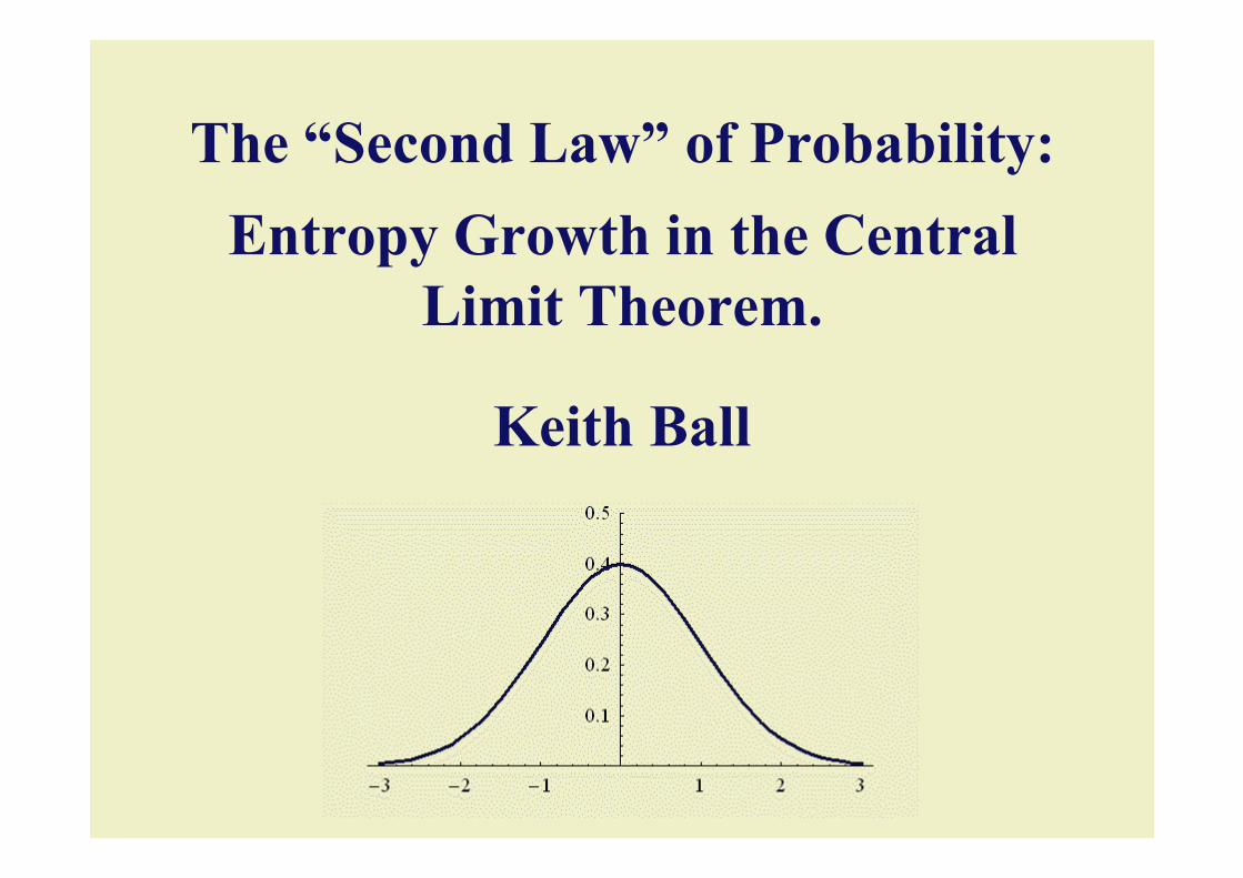
The “Second Law” of Probability:Entropy Growth in the Central
Limit Theorem.
Keith Ball

The second law of thermodynamics
Joule and Carnot studied ways to improve theefficiency of steam engines.
Is it possible for a thermodynamic system to move fromstate A to state B without any net energy being put into thesystem from outside?
A single experimental quantity, dubbed entropy, made itpossible to decide the direction of thermodynamic changes.
The second law of thermodynamics
The entropy of a closed system increases with time.
The second law applies to all changes: not justthermodynamic.
Entropy measures the extent to which energy is dispersed:so the second law states that energy tends to disperse.
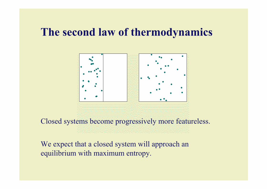
The second law of thermodynamics
Closed systems become progressively more featureless.
We expect that a closed system will approach anequilibrium with maximum entropy.
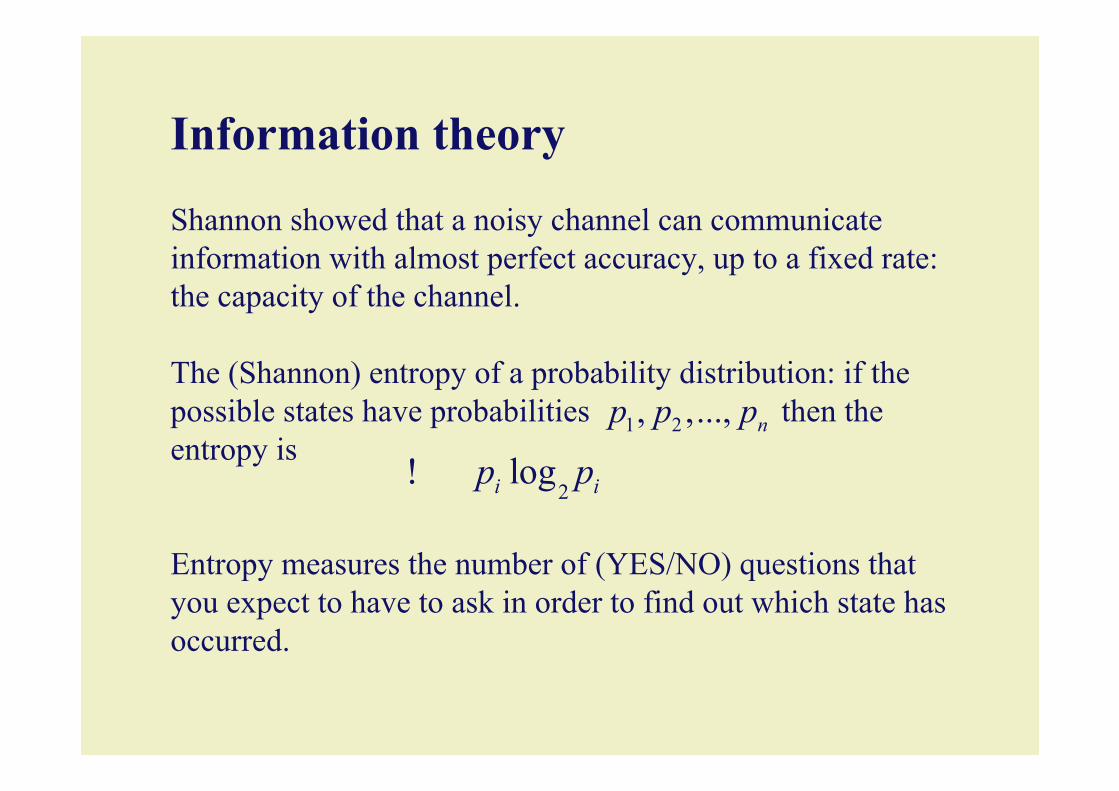
Information theory
Shannon showed that a noisy channel can communicateinformation with almost perfect accuracy, up to a fixed rate:the capacity of the channel.
The (Shannon) entropy of a probability distribution: if thepossible states have probabilities then theentropy is
Entropy measures the number of (YES/NO) questions thatyou expect to have to ask in order to find out which state hasoccurred.
1 2, ,..., np p p
2logi ip p!

Information theory
You can distinguish 2k
states with k (YES/NO)questions.
If the states are equallylikely, then this is thebest you can do.
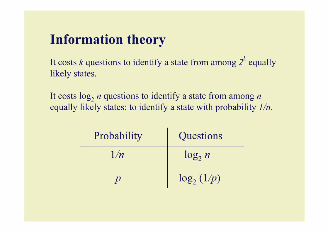
It costs k questions to identify a state from among 2k equallylikely states.
Information theoryIt costs k questions to identify a state from among 2k equallylikely states.
It costs log2 n questions to identify a state from among nequally likely states: to identify a state with probability 1/n.
log2 (1/p) p
log2 n 1/n
Questions Probability
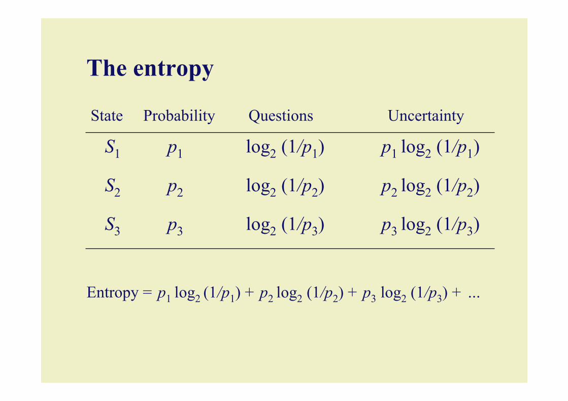
p3 log2 (1/p3) log2 (1/p3) p3 S3
p2 log2 (1/p2) log2 (1/p2) p2 S2
p1 log2 (1/p1) log2 (1/p1) p1 S1
Uncertainty Questions ProbabilityState
Entropy = p1 log2 (1/p1) + p2 log2 (1/p2) + p3 log2 (1/p3) + …
The entropy

Continuous random variables
For a random variable X with density f the entropy is
The entropy behaves nicely under several naturalprocesses: for example, the evolution governed by theheat equation.
( )Ent logX f f= !
10

If the density f measures the distribution of heat in an infinitemetal bar, then f evolves according to the heat equation:
The entropy increases:
''f ft!
=!
( )2'log 0ff ft f
! = #
!
Fisher information
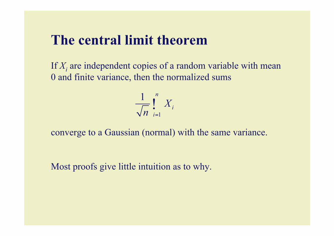
The central limit theorem
If Xi are independent copies of a random variable with mean0 and finite variance, then the normalized sums
converge to a Gaussian (normal) with the same variance.
Most proofs give little intuition as to why.
1
1 n
iiX
n =!

The central limit theoremAmong random variables with a given variance, the Gaussianhas largest entropy.
Theorem (Shannon-Stam) If X and Y are independent andidentically distributed, then the normalized sum
has entropy at least that of X and Y.2
X Y+

Idea
The central limit theorem is analogous to the second law ofthermodynamics: the normalized sums
have increasing entropy which drives them to an“equilibrium” which has maximum entropy.
1
1 n
n ii
S Xn =
= !
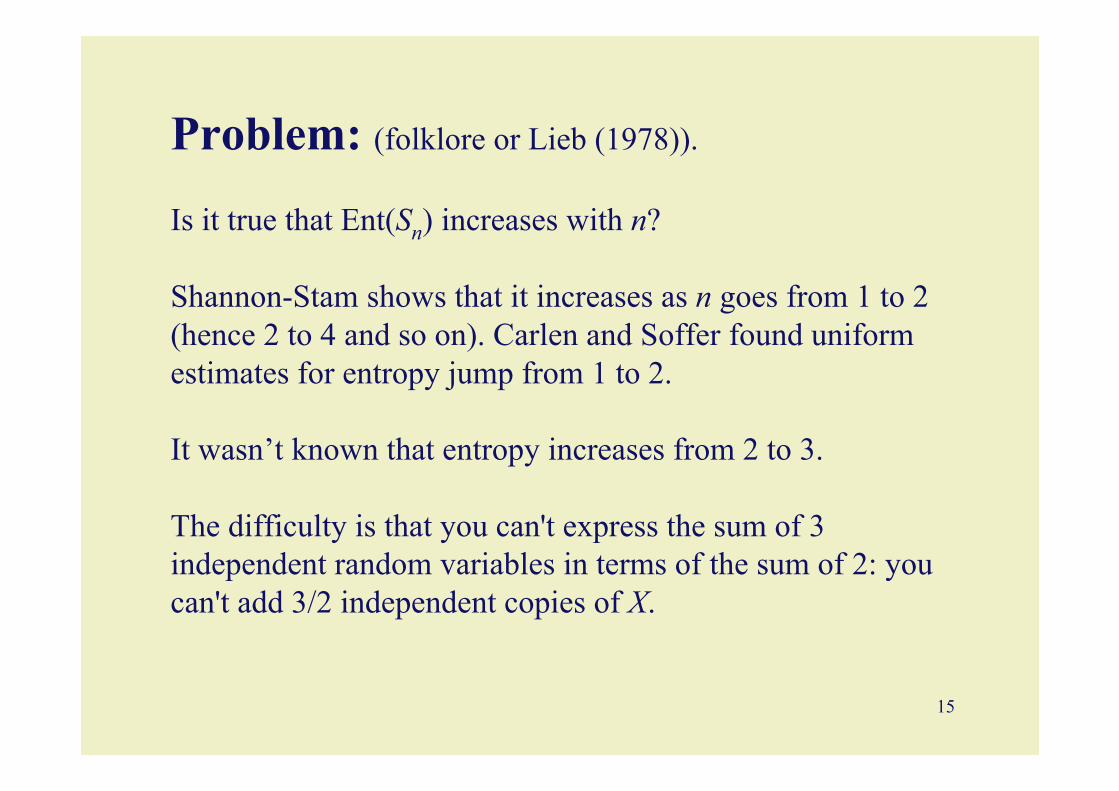
Problem: (folklore or Lieb (1978)).
Is it true that Ent(Sn) increases with n?
Shannon-Stam shows that it increases as n goes from 1 to 2(hence 2 to 4 and so on). Carlen and Soffer found uniformestimates for entropy jump from 1 to 2.
It wasn’t known that entropy increases from 2 to 3.
The difficulty is that you can't express the sum of 3independent random variables in terms of the sum of 2: youcan't add 3/2 independent copies of X.
15
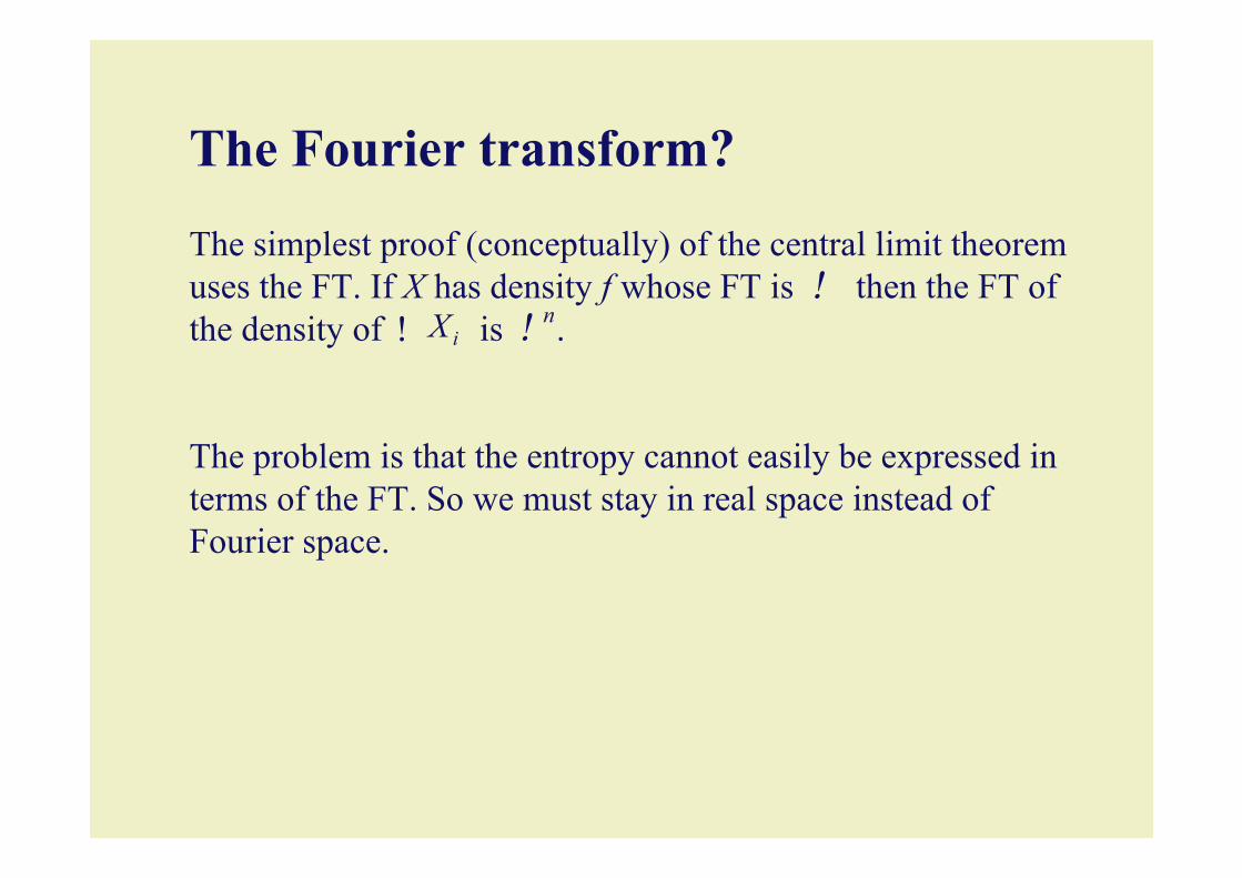
The Fourier transform?
The simplest proof (conceptually) of the central limit theoremuses the FT. If X has density f whose FT is then the FT ofthe density of is .
The problem is that the entropy cannot easily be expressed interms of the FT. So we must stay in real space instead ofFourier space.
iX!!
n!
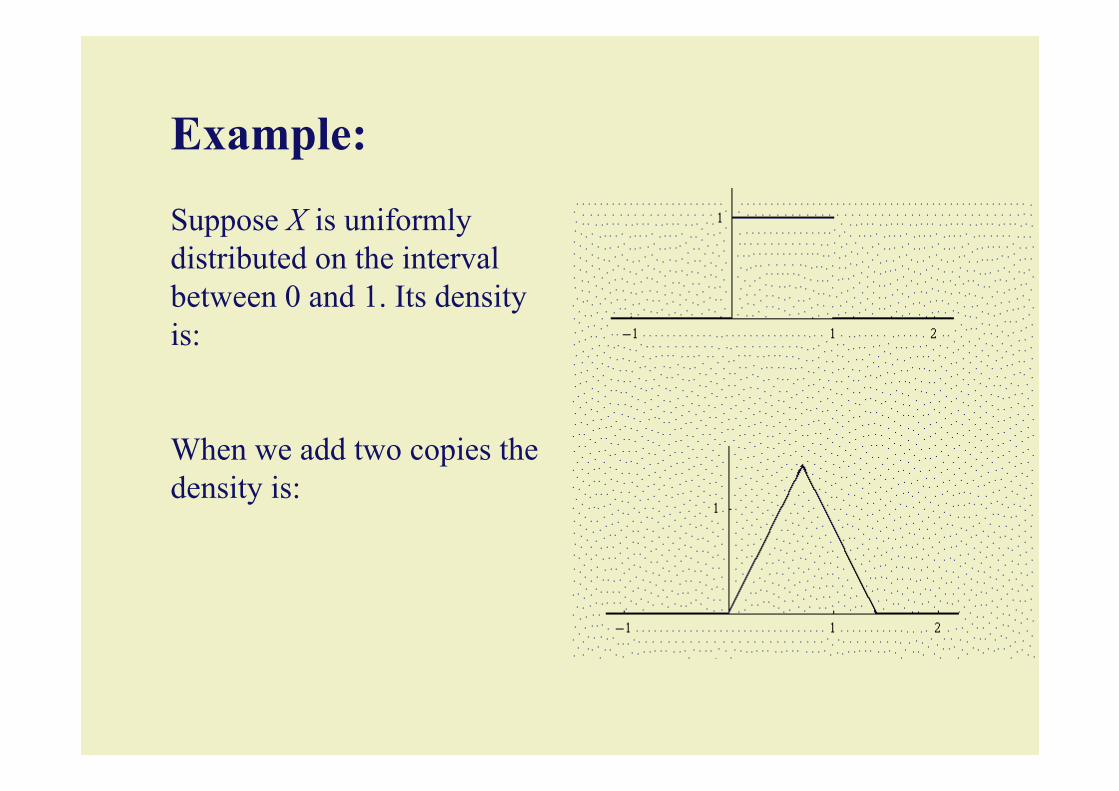
Example:
Suppose X is uniformlydistributed on the intervalbetween 0 and 1. Its densityis:
When we add two copies thedensity is:
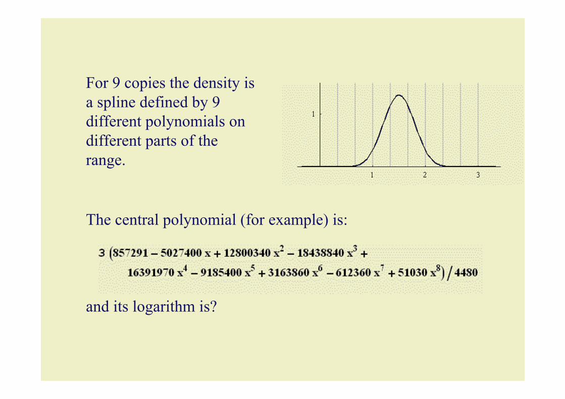
For 9 copies the density isa spline defined by 9different polynomials ondifferent parts of therange.
The central polynomial (for example) is:
and its logarithm is?
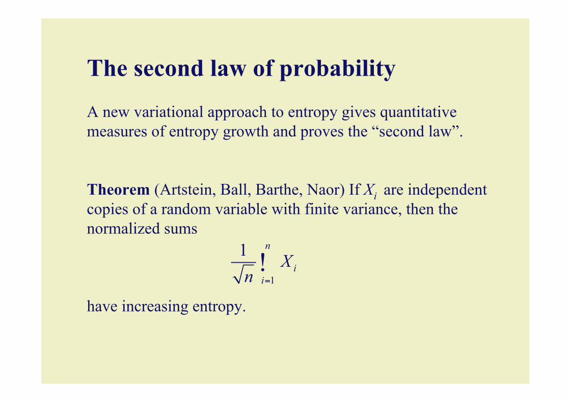
A new variational approach to entropy gives quantitativemeasures of entropy growth and proves the “second law”.
Theorem (Artstein, Ball, Barthe, Naor) If Xi are independentcopies of a random variable with finite variance, then thenormalized sums
have increasing entropy.
1
1 n
iiX
n =!
The second law of probability

Starting point: used by many authors. Instead ofconsidering entropy directly, we study the Fisher information:
Among random variables with variance 1, the Gaussianhas the smallest Fisher information, namely 1.
The Fisher information should decrease as a process evolves.
2'( ) ff
J X = !
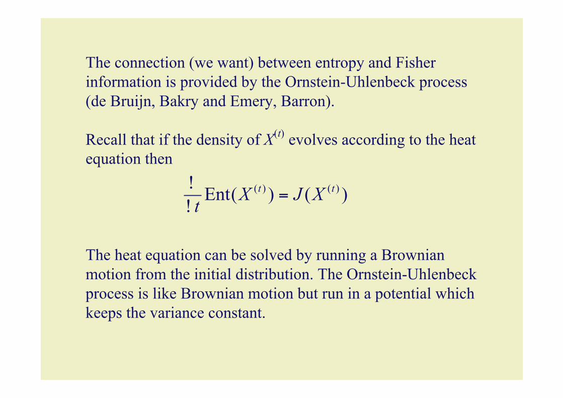
The connection (we want) between entropy and Fisherinformation is provided by the Ornstein-Uhlenbeck process(de Bruijn, Bakry and Emery, Barron).
Recall that if the density of X(t) evolves according to the heatequation then
The heat equation can be solved by running a Brownianmotion from the initial distribution. The Ornstein-Uhlenbeckprocess is like Brownian motion but run in a potential whichkeeps the variance constant.
( ) ( )Ent( ) ( )t tX J Xt!
=!
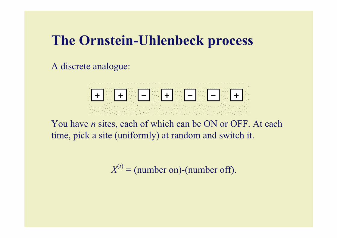
The Ornstein-Uhlenbeck process
A discrete analogue:
You have n sites, each of which can be ON or OFF. At eachtime, pick a site (uniformly) at random and switch it.
X(t) = (number on)-(number off).

The Ornstein-Uhlenbeck process
A typical path of the process.

The Ornstein-Uhlenbeck evolution
The density evolves according to the modified diffusionequation:
From this:
As the evolutes approach the Gaussian of the samevariance.
'' ( ) 'f f xft!
= +!
( ) ( )Ent( ) ( ) 1t tX J Xt!
= !
t !
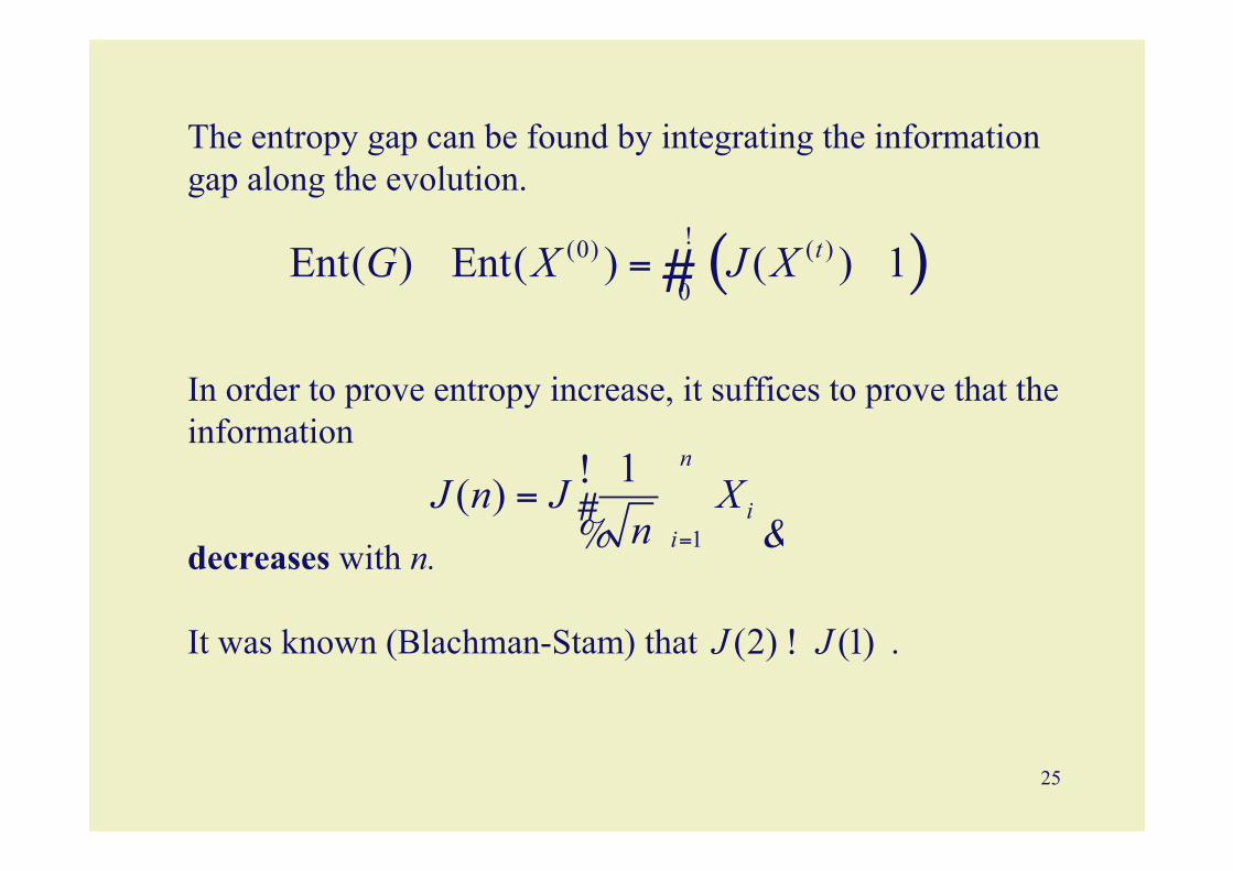
The entropy gap can be found by integrating the informationgap along the evolution.
In order to prove entropy increase, it suffices to prove that theinformation
decreases with n.
It was known (Blachman-Stam) that .
1
1( )n
ii
J n J Xn =
! = #
% &
(2) (1)J J!
( )(0) ( )
0Ent( ) Ent( ) ( ) 1tG X J X
! = #
25

Main new tool: a variational description of theinformation of a marginal density.
If w is a density on and e is a unit vector, then the marginalin direction e has density
n
( )te e
h t w!+=

Main new tool:
2 2'( ) '( )''( ) ( log ) ''
( ) ( )( ) h t h t
h t h hh t h t
J h !!= = =
The density h is a marginal of w and
The integrand is non-negative if h has concave logarithm.
Densities with concave logarithm have been widely studied inhigh-dimensional geometry, because they naturally generalizeconvex solids.

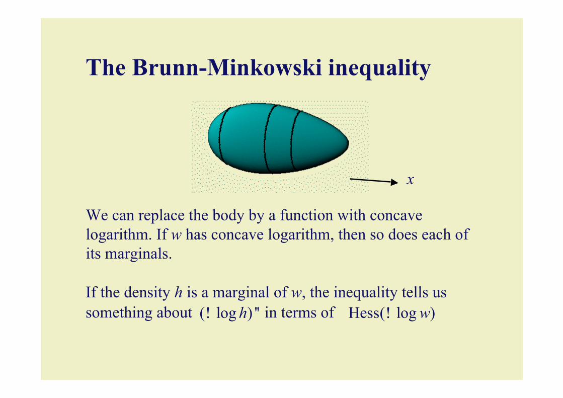
The Brunn-Minkowski inequality
Let A(x) be the cross-sectional area of a convex body atposition x.
Then log A is concave.
The function A is a marginal of the body.
x
The Brunn-Minkowski inequality
We can replace the body by a function with concavelogarithm. If w has concave logarithm, then so does each ofits marginals.
x
If the density h is a marginal of w, the inequality tells ussomething about in terms of( log ) ''h! Hess( log )w!
The Brunn-Minkowski inequality
If the density h is a marginal of w, the inequality tells ussomething about in terms of( log ) ''h! Hess( log )w!
We rewrite a proof of the Brunn-Minkowski inequality soas to provide an explicit relationship between the two. Theexpression involving the Hessian is a quadratic formwhose minimum is the information of h.
This gives rise to the variational principle.
30
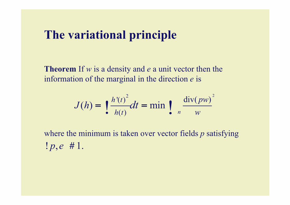
The variational principle
Theorem If w is a density and e a unit vector then theinformation of the marginal in the direction e is
where the minimum is taken over vector fields p satisfying, 1.p e! #
22'( )
( )
div( )( ) minn
h t
h t
pww
J h dt= =! !

Technically we have gained because h(t) is an integral: notgood in the denominator.
The real point is that we get to choose p. Instead ofchoosing the optimal p which yields the intractableformula for information, we choose a non-optimal p withwhich we can work.
22'( )
( )
div( )( ) minn
h t
h t
pww
J h dt= =! !

Proof of the variational principle.
so
If p satisfies at each point, then we can realisethe derivative as
since the part of the divergence perpendicular to eintegrates to 0 by the Gauss-Green (divergence) theorem.
'( ) ete eh t w!+
= #
, 1p e! #
'( ) div( )te e
h t pw!+=
( )te e
h t w!+=
( ) 22
2
'( )
( )
div( ) div( )te e
n
h t
h t w
pw pww
dt dt!+ # =%
%% % %
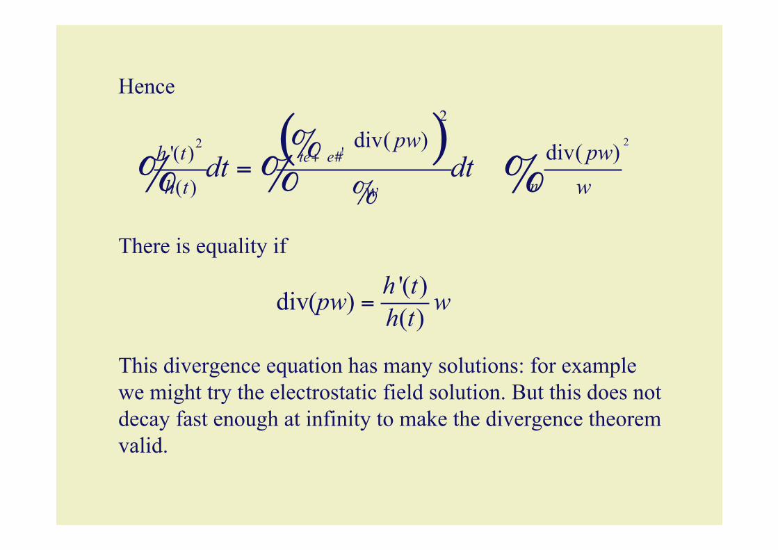
Hence
There is equality if
This divergence equation has many solutions: for examplewe might try the electrostatic field solution. But this does notdecay fast enough at infinity to make the divergence theoremvalid.
'( )div( ) ( )h tpw wh t=
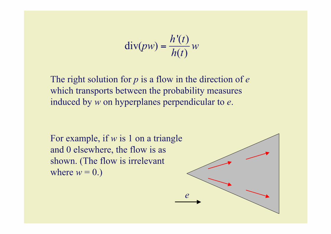
'( )div( ) ( )h tpw wh t=
The right solution for p is a flow in the direction of ewhich transports between the probability measuresinduced by w on hyperplanes perpendicular to e.
For example, if w is 1 on a triangleand 0 elsewhere, the flow is asshown. (The flow is irrelevantwhere w = 0.)
e

Theorem If Xi are independent copies of a random variablewith variance, then the normalized sums
have increasing entropy.1
1 n
iiX
n =!
The second law of probability

![OPEN ACCESS entropy · 2017. 5. 7. · Entropy 2012, 14 1607 1. Introduction The first notion of entropy of a probability distribution was addressed by [1], thus becoming a measure](https://static.fdocuments.us/doc/165x107/5fbcc2e0e98923492a75786e/open-access-entropy-2017-5-7-entropy-2012-14-1607-1-introduction-the-irst.jpg)