THE SCIENCE AND INFORMATION ORGANIZATION
54
Transcript of THE SCIENCE AND INFORMATION ORGANIZATION


THE SCIENCE AND INFORMATION ORGANIZATION
www.thesa i .o rg | in fo@thesa i .o rg
INTERNATIONAL JOURNAL OFADVANCED RESEARCH IN ARTIFICIAL INTELLIGENCE

(IJARAI) International Journal of Advanced Research in Artificial Intelligence,
Vol. 1, No. 3, 2012
(i)
www.ijarai.thesai.org
Editorial Preface
From the Desk of Managing Editor…
“The question of whether computers can think is like the question of whether submarines can swim.”
― Edsger W. Dijkstra, the quote explains the power of Artificial Intelligence in computers with the changing
landscape. The renaissance stimulated by the field of Artificial Intelligence is generating multiple formats
and channels of creativity and innovation. This journal is a special track on Artificial Intelligence by The
Science and Information Organization and aims to be a leading forum for engineers, researchers and
practitioners throughout the world.
The journal reports results achieved; proposals for new ways of looking at AI problems and include
demonstrations of effectiveness. Papers describing existing technologies or algorithms integrating multiple
systems are welcomed. IJARAI also invites papers on real life applications, which should describe the current
scenarios, proposed solution, emphasize its novelty, and present an in-depth evaluation of the AI
techniques being exploited. IJARAI focusses on quality and relevance in its publications. In addition, IJARAI
recognizes the importance of international influences on Artificial Intelligence and seeks international input
in all aspects of the journal, including content, authorship of papers, readership, paper reviewers, and
Editorial Board membership.
In this issue we have contributions on method for learning efficiency improvements based on gaze location
notifications on e-learning content screen display; hybrid metaheuristics for the unrelated parallel machine
scheduling to minimize makespan and maximum just-in-time deviations; fuzzy controller design using fpga
for photovoltaic maximum power point tracking; automated detection method for clustered
microcalcification in mammogram image based on statistical textural features; temperature control system
using fuzzy logic technique; a new genetic algorithm based lane-by-pass approach for smooth traffic flow
on road networks; leaf image segmentation based on the combination of wavelet transform and k means
clustering; and also poultry diseases warning system using dempster-shafer theory and web mapping
The success of authors and the journal is interdependent. While the Journal is in its initial phase, it is not only
the Editor whose work is crucial to producing the journal. The editorial board members , the peer reviewers,
scholars around the world who assess submissions, students, and institutions who generously give their
expertise in factors small and large— their constant encouragement has helped a lot in the progress of the
journal and shall help in future to earn credibility amongst all the reader members. I add a personal thanks
to the whole team that has catalysed so much, and I wish everyone who has been connected with the
Journal the very best for the future.
Thank you for Sharing Wisdom!
Managing Editor
IJARAI
Volume 1 Issue 3 June 2012
ISSN: 2165-4069(Online)
ISSN: 2165-4050(Print)
©2012 The Science and Information (SAI) Organization

(IJARAI) International Journal of Advanced Research in Artificial Intelligence,
Vol. 1, No. 3, 2012
(ii)
www.ijarai.thesai.org
Associate Editors
Dr.T. V. Prasad
Dean (R&D), Lingaya's University, India
Domain of Research: Bioinformatics, Natural Language Processing, Image Processing,
Robotics, Knowledge Representation
Dr.Wichian Sittiprapaporn
Senior Lecturer, Mahasarakham University, Thailand
Domain of Research: Cognitive Neuroscience; Cognitive Science
Prof.Alaa Sheta
Professor of Computer Science and Engineering, WISE University, Jordan
Domain of Research: Artificial Neural Networks, Genetic Algorithm, Fuzzy Logic Theory,
Neuro-Fuzzy Systems, Evolutionary Algorithms, Swarm Intelligence, Robotics
Dr.Yaxin Bi
Lecturer, University of Ulster, United Kingdom
Domain of Research: Ensemble Learing/Machine Learning, Multiple Classification
Systesm, Evidence Theory, Text Analytics and Sentiment Analysis
Mr.David M W Powers
Flinders University, Australia
Domain of Research: Language Learning, Cognitive Science and Evolutionary Robotics,
Unsupervised Learning, Evaluation, Human Factors, Natural Language Learning,
Computational Psycholinguistics, Cognitive Neuroscience, Brain Computer Interface,
Sensor Fusion, Model Fusion, Ensembles and Stacking, Self-organization of Ontologies,
Sensory-Motor Perception and Reactivity, Feature Selection, Dimension Reduction,
Information Retrieval, Information Visualization, Embodied Conversational Agents
Dr.Antonio Dourado
University of Coimbra, France
Domain of Research: Computational Intelligence, Signal Processing, data mining for
medical and industrial applications, and intelligent control.

(IJARAI) International Journal of Advanced Research in Artificial Intelligence,
Vol. 1, No. 3, 2012
(iii)
www.ijarai.thesai.org
Reviewer Board Members
Alaa Sheta
WISE University
Albert Alexander
Kongu Engineering College
Amir HAJJAM EL HASSANI
Université de Technologie de Belfort-Monbéliard
Amit Verma
Department in Rayat & Bahra Engineering
College,Mo
Antonio Dourado
University of Coimbra
B R SARATH KUMAR
LENORA COLLEGE OF ENGINEERNG
Babatunde Opeoluwa Akinkunmi
University of Ibadan Bestoun S.Ahmed
Universiti Sains Malaysia
David M W Powers
Flinders University
Dhananjay Kalbande
Mumbai University
Dipti D. Patil
MAEERs MITCOE Francesco Perrotta
University of Macerata
Grigoras Gheorghe
"Gheorghe Asachi" Technical University of Iasi,
Romania
Guandong Xu
Victoria University
Jatinderkumar R. Saini
S.P.College of Engineering, Gujarat Krishna Prasad Miyapuram
University of Trento
Marek Reformat
University of Alberta
Md. Zia Ur Rahman
Narasaraopeta Engg. College, Narasaraopeta
Mohd Helmy Abd Wahab
Universiti Tun Hussein Onn Malaysia
Nitin S. Choubey
Mukesh Patel School of Technology
Management & Eng
Rajesh Kumar
National University of Singapore
Rajesh K Shukla
Sagar Institute of Research & Technology-
Excellence, Bhopal MP
Sana'a Wafa Tawfeek Al-Sayegh
University College of Applied Sciences
Saurabh Pal
VBS Purvanchal University, Jaunpur
Shaidah Jusoh
Zarqa University
SUKUMAR SENTHILKUMAR
Universiti Sains Malaysia T. V. Prasad
Lingaya's University VUDA Sreenivasarao
St. Mary’s College of Engineering & Technology
Wei Zhong
University of south Carolina Upstate
Wichian Sittiprapaporn
Mahasarakham University
Yaxin Bi
University of Ulster
Yuval Cohen
The Open University of Israel
Zhao Zhang
Deptment of EE, City University of Hong Kong Zne-Jung Lee
Dept. of Information management, Huafan
University

(IJARAI) International Journal of Advanced Research in Artificial Intelligence,
Vol. 1, No. 3, 2012
(iv)
www.ijarai.thesai.org
CONTENTS
Paper 1: Method for Learning Effciency Improvements Based on Gaze Location Notifications on e-learning Content
Screen Display
Authors: Kohei Arai
PAGE 1 – 6
Paper 2: Hybrid Metaheuristics for the Unrelated Parallel Machine Scheduling to Minimize Makespan and Maximum Just-
in-Time Deviations
Authors: Chiuh-Cheng Chyu, Wei-Shung Chang
PAGE 7 – 13
Paper 3: Fuzzy Controller Design Using FPGA for Photovoltaic Maximum Power Point Tracking
Authors: Basil M. Hamed, Mohammed S. El-Moghany
PAGE 14 – 21
Paper 4: Automated Detection Method for Clustered Microcalcification in Mammogram Image Based on Statistical
Textural Features
Authors: Kohei Arai, Indra Nugraha Abdullah, Hiroshi Okumura
PAGE 22 – 26
Paper 5: Temperature Control System Using Fuzzy Logic Technique
Authors: Isizoh A. N., Okide S. O, Anazia A.E. Ogu C.D.
PAGE 27 – 31
Paper 6: A New Genetic Algorithm Based Lane-By-Pass Approach for Smooth Traffic Flow on Road Networks
Authors: Shailendra Tahilyani, Manuj Darbari, Praveen Kumar Shukla
PAGE 32 – 36
Paper 7: Leaf Image Segmentation Based On the Combination of Wavelet Transform and K Means Clustering
Authors: N.Valliammal, Dr.S.N.Geethalakshmi
PAGE 37 – 43
Paper 8: Poultry Diseases Warning System using Dempster-Shafer Theory and Web Mapping
Authors: Andino Maseleno, Md. Mahmud Hasan
PAGE 44 – 48

(IJARAI) International Journal of Advanced Research in Artificial Intelligence,
Vol. 1, No. 3, 2012
1 | P a g e
www.ijarai.thesai.org
Method for Learning Effciency Improvements Based
on Gaze Location Notifications on e-learning Content
Screen Display
Kohei Arai
Graduate School of Science and Engineering
Saga University
Saga City, Japan
Abstract— Method for learning efficiency improvement based on
gaze notifications on e-learning content screen display is
proposed. Experimental results with e-learning two types of
contents (Relatively small motion of e-learning content and e-
learning content with moving picture and annotation marks)
show that 0.8038 to 0.9615 of R square value are observed
between duration time period of proper gaze location and
achievement test score.
Keywords- Gaze estimation; e-learning content; thesaurus engine.
I. INTRODUCTION
Computer key-in system by human eyes only (just by sight) is proposed [1],[2]. The system allows key-in when student looks at the desired key (for a while or with blink) in the screen keyboard displayed onto computer screen. Also blink detection accuracy had to be improved [3],[4]. Meanwhile, influence due to students' head pose, different cornea curvature for each student, illumination conditions, background conditions, reflected image (environmental image) on students' eyes, eyelashes affecting to pupil center detection, un-intentional blink, etc. are eliminated for gaze detection accuracy improvement [5],[6]. On the other hands, the system is applied for communication aid, having meal aid, electric wheel chair control, content access aid (e-learning, e-comic, e-book), phoning aid, Internet access aid (including Web search), TV watching aid, radio listening aid, and so on [7]-[17].
The method for key-in accuracy improvement with moving screen keyboard is also proposed [18]. Only thing student has to do is looking at one of the following five directions, center, top, bottom, left and right so that key-in accuracy is remarkably improved (100% perfect) and student can use the system in a relax situation.
One of the applications of gaze estimation is attempted in this study. Using gaze estimation method, lecturers can monitor the screen location where students are looking at during they are learning. Sometime students are not looking at the same location where content creator would like students look at. Such students may fail or have a bad score in achievement tests. When students learn with e-learning contents, lecturers can monitor their gaze location so that lecturers may give a caution when students are looking at somewhere else from the location where lecturers would like students look at. Thus learning efficiency may improve
somewhat.
The second section describes the proposed system followed by some experimental results. In the experiments, learning with typical e-learning content with gaze estimation is conducted first followed by learning with e-learning contents of moving picture with annotations (lecturer indicates the location where lecturer would like students look at with some marks). Thus effectiveness of the e-learning with gaze estimation is enhanced. Finally, concluding remarks are followed by with some discussions.
II. PROPOSED SYSTEM
A. Gaze Location Estimation Method and System
Students wear a two Near Infrared: NIR cameras (NetCowBoy, DC-NCR130
1) mounted glass. One camera
acquires student eye while the other camera acquires computer screen which displays e-learning content. Outlook of the glass is shown in Figure 1 while the specification of NIR camera is shown in Table 1, respectively.
Figure 1. Proposed glass with two NIR cameras
TABLE I. SPECIFICATION OF NIR CAMERA
Resolution 1,300,000pixels
Minimum distance 20cm
Frame rate 30fps
Minimum illumination 30lx
Size 52mm(W)x70mm(H)x65mm(D)
Weight 105g
In order to monitor students' psychological situation, Electroencephalography: eeg
2 sensor (NueroSky
3) is also
attached to students' forehead as shown in Figure 2.
1 http://www.digitalcowboy.jp/support/drivers/dc-ncr130/index.html
2 http://en.wikipedia.org/wiki/Electroencephalography
3 http://www.neurosky.com/
(IJARAI) International Journal of Advanced Research in Artificial Intelligence,
Vol. 1, No. 3, 2012
2 | P a g e
www.ijarai.thesai.org
Figure 2. NeuroSky of EEG sensor
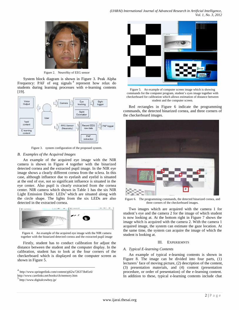
System block diagram is shown in Figure 3. Peak Alpha Frequency: PAF of eeg signals
4 represent how relax do
students during learning processes with e-learning contents [19].
Figure 3. system configuration of the proposed system.
B. Examples of the Acquired Images
An example of the acquired eye image with the NIR camera is shown in Figure 4 together with the binarized detected cornea and the extracted pupil image. In the NIR eye image shows a clearly different cornea from the sclera. In this case, although influence due to eyelash and eyelid is situated at the end of eye, not so significant influence is situated in the eye center. Also pupil is clearly extracted from the cornea center. NIR camera which shown in Table 1 has the six NIR Light Emission Diode: LEDs
5 which are situated along with
the circle shape. The lights from the six LEDs are also detected in the extracted cornea.
Figure 4. An example of the acquired eye image with the NIR camera
together with the binarized detected cornea and the extracted pupil image
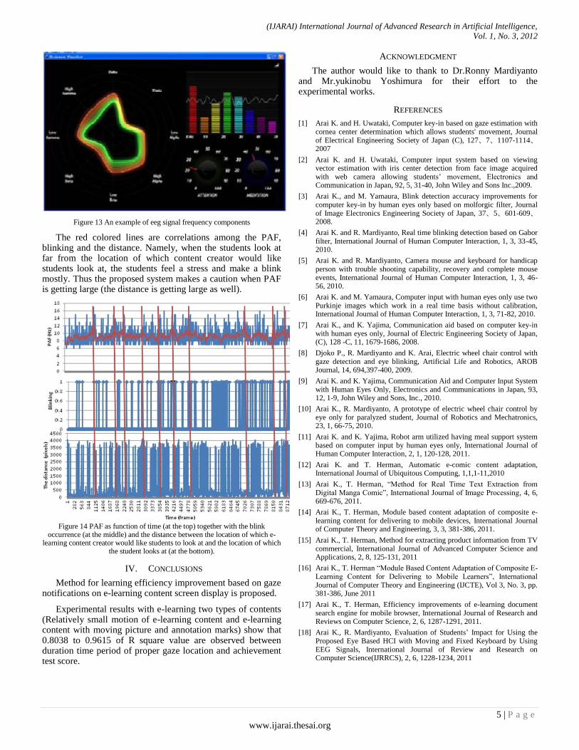
Firstly, student has to conduct calibration for adjust the distance between the student and the computer display. In the calibration, student has to look at the four corners of the checkerboard which is displayed on the computer screen as shown in Figure 5.
4 http://www.springerlink.com/content/pj62w726373h45x6/
http://www.carelinks.net/books/ch/memory.htm 5 http://www.digitalcowboy.jp/
Figure 5. An example of computer screen image which is showing
commands for the computer program, student’s eyes image together with
checkerboard for calibration which allows estimation of distance between
student and the computer screen.
Red rectangles in Figure 6 indicate the programming commands, the detected binarized cornea, and three corners of the checkerboard images.
Figure 6. The programming commands, the detected binarized cornea, and
three corners of the checkerboard images.
Two images which are acquired with the camera 1 for student’s eye and the camera 2 for the image of which student is now looking at. At the bottom right in Figure 7 shows the image which is acquired with the camera 2. With the camera 1 acquired image, the system can estimate the gaze location. At the same time, the system can acquire the image of which the student is looking at.
III. EXPERIEMNTS
A. Typical E-learning Contents
An example of typical e-learning contents is shown in Figure 8. The image can be divided into four parts, (1) lecturers’ face of moving picture, (2) description of the content, (3) presentation materials, and (4) content (presentation procedure, or order of presentation) of the e-learning content. In addition to these, typical e-learning contents include chat

(IJARAI) International Journal of Advanced Research in Artificial Intelligence,
Vol. 1, No. 3, 2012
3 | P a g e
www.ijarai.thesai.org
and Bulletin Board System: BBS6 for Question and Answer
(Q/A). Usually, content creators would like student to look at the description and the presentation material back and forth. Students, however, used to look at the different location other than the description and the presentation material. Such those students cannot learn effectively.
Figure 7. An example of the image which is acquired with the camera 2 at
the bottom right.
The proposed system allows identifications of the location of which student is looking at. Also students can hear lecturers voice of instructions.
Therefore, students can concentrate the presentation materials and the descriptions much more by referring to the difference between the location of which students are looking at and supposed location of which content creator would like students look at.
10 of students have to have achievement test with 12 questions. In this case of the typical e-learning content, (2) of the portion, description of the content is the most appropriate portion of which students would better to look at. Table 2 shows the achievement test score and the time duration for which students are looking at one of the four different portions.
For instance, student No.1 looks at the portion no.2 (descriptions of the content) for 10 unit time followed by the portion no.1 (lecturers’ face) for 4 unit time, the portion no.3 (presentation materials) for 3 unit time, and the portion no.4 (The other portion) for 2 unit time.
Figure 9 shows relation between the achievement test results and duration time. There is a good correlation between the score and the duration time for which the students are looking at the portion no.2 (R square value
7 of 0.9615). There
are no such high correlations between the score and the duration time for which the students are looking at the portions other than the portion no.2.
6
http://ja.wikipedia.org/wiki/%E9%9B%BB%E5%AD%90%E6%8E%B2%E7
%A4%BA%E6%9D%BF 7 http://en.wikipedia.org/wiki/Coefficient_of_determination
Figure 8. An example of typical e-learning contents (The image can be divided into four parts, (1) lecturers’ face of moving picture, (2) description of
the content, (3) presentation materials, and (4) content (presentation procedure, or order of presentation) of the e-learning content.
TABLE II. SHOWS THE ACHIEVEMENT TEST SCORE AND THE TIME
DURATION FOR WHICH STUDENTS ARE LOOKING AT ONE OF THE FOUR
PORTIONS.
Student No. Score 1 2 3 4
1 11 4 10 3 2
2 10 4 9 5 1
3 10 5 9 3 2
4 8 5 8 4 2
5 8 6 7 3 3
6 8 5 7 6 1
7 7 6 6 5 2
8 6 6 5 4 4
9 6 4 6 5 4
10 4 6 3 4 6
Figure 9. shows relation between the achievement test results and duration
time.
B. E-learning Contents withMoving Picture and the
Annotations
There are a plenty of e-learning contents featuring moving pictures with annotations. Lecture is provided in accordance

(IJARAI) International Journal of Advanced Research in Artificial Intelligence,
Vol. 1, No. 3, 2012
4 | P a g e
www.ijarai.thesai.org
with presentation materials with annotation of marks (hand written, sometime) and lecturers’ face. Figure 10 shows such example of e-learning contents. In this example, lecturer makes handwritten marks at the appropriate time and locations. There are two major portions, the portion #1 (presentation materials) and the portions #2 (Lecturer’s face). The portion #1 is divided into the portion no.1 and the portion no.2. The portion no.1 denotes the appropriate location where the locations are marked while the portion no.2 denotes the other locations in the portion #1. The portion no.3 denotes lecturer’s face while the portion no.4 denotes the other locations out of the portion #1 and #2.
Figure 10. An example of e-learning contents (lecturer makes handwritten
marks at the appropriate time and locations).
Relation between the score of the achievement test and the portions where the students are looking at is shown in Table 3. It is quite obvious that there is strong correlation between the score and the duration time for the portion no.1. Therefore, it may say that the score is excellent if the students look at the appropriate portions, in particular, marked portions in the presentation materials. The time period of learning with this e-learning content is 22 unit time. The highest score is made by the student who looks at the appropriate portions for 16 unit time out of 22 unit time.
TABLE III. RELATION BETWEEN THE SCORE OF THE ACHIEVEMENT TEST
AND THE PORTIONS WHERE THE STUDENTS ARE LOOKING AT
Student Score 1 2 3 4
1 10 16 3 2 1
2 10 15 4 2 1
3 10 14 3 1 4
4 9 14 2 5 1
5 8 13 4 3 2
6 8 13 4 2 3
7 8 12 3 3 4
8 7 13 2 5 2
9 6 11 5 4 2
10 6 9 4 4 5 Correlation between the score and the portion no.1 where
the students is looking at is around 0.8038 of R square value as shown in Figure 11.
Figure 11. Correlation between the score and the portion no.1 where the
students is looking at is around 0.8038 of R square value
C. Reading Types of E-learning Content
One of the examples of reading types of e-learning contents is shown in Figure 12. In this example, the location of which e-learning content creator would like students to look at is marked with black circle while the location of which the student looks at is marked with green circle.
The distance between both locations can be calculated. If the accumulated distance exceeds a prior determined threshold, then some caution is made by the proposed system. Thus the student may follow the desirable locations.
Figure 12 One of the examples of reading types of e-learning contents
D. Monitoring Students’ Psycological Status
In order to check students’ psychological statue during learning with reading type of e-learning contents, Peak Alpha Frequency: PAF of eeg signal is evaluated.
An example of eeg signal frequency components is illustrated in Figure 13. Also the PAF as function of time is shown in the top of Figure 14 together with the blink occurrence (at the middle) and the distance between the location of which e-learning content creator would like students to look at and the location of which the student looks at (at the bottom).
(IJARAI) International Journal of Advanced Research in Artificial Intelligence,
Vol. 1, No. 3, 2012
5 | P a g e
www.ijarai.thesai.org
Figure 13 An example of eeg signal frequency components
The red colored lines are correlations among the PAF, blinking and the distance. Namely, when the students look at far from the location of which content creator would like students look at, the students feel a stress and make a blink mostly. Thus the proposed system makes a caution when PAF is getting large (the distance is getting large as well).
Figure 14 PAF as function of time (at the top) together with the blink
occurrence (at the middle) and the distance between the location of which e-learning content creator would like students to look at and the location of which
the student looks at (at the bottom).
IV. CONCLUSIONS
Method for learning efficiency improvement based on gaze notifications on e-learning content screen display is proposed.
Experimental results with e-learning two types of contents (Relatively small motion of e-learning content and e-learning content with moving picture and annotation marks) show that 0.8038 to 0.9615 of R square value are observed between duration time period of proper gaze location and achievement test score.
ACKNOWLEDGMENT
The author would like to thank to Dr.Ronny Mardiyanto and Mr.yukinobu Yoshimura for their effort to the experimental works.
REFERENCES
[1] Arai K. and H. Uwataki, Computer key-in based on gaze estimation with cornea center determination which allows students' movement, Journal of Electrical Engineering Society of Japan (C), 127、7、1107-1114、2007
[2] Arai K. and H. Uwataki, Computer input system based on viewing vector estimation with iris center detection from face image acquired with web camera allowing students’ movement, Electronics and Communication in Japan, 92, 5, 31-40, John Wiley and Sons Inc.,2009.
[3] Arai K., and M. Yamaura, Blink detection accuracy improvements for computer key-in by human eyes only based on molforgic filter, Journal of Image Electronics Engineering Society of Japan, 37、5、601-609、2008.
[4] Arai K. and R. Mardiyanto, Real time blinking detection based on Gabor filter, International Journal of Human Computer Interaction, 1, 3, 33-45, 2010.
[5] Arai K. and R. Mardiyanto, Camera mouse and keyboard for handicap person with trouble shooting capability, recovery and complete mouse events, International Journal of Human Computer Interaction, 1, 3, 46-56, 2010.
[6] Arai K. and M. Yamaura, Computer input with human eyes only use two Purkinje images which work in a real time basis without calibration, International Journal of Human Computer Interaction, 1, 3, 71-82, 2010.
[7] Arai K., and K. Yajima, Communication aid based on computer key-in with human eyes only, Journal of Electric Engineering Society of Japan, (C), 128 -C, 11, 1679-1686, 2008.
[8] Djoko P., R. Mardiyanto and K. Arai, Electric wheel chair control with gaze detection and eye blinking, Artificial Life and Robotics, AROB Journal, 14, 694,397-400, 2009.
[9] Arai K. and K. Yajima, Communication Aid and Computer Input System with Human Eyes Only, Electronics and Communications in Japan, 93, 12, 1-9, John Wiley and Sons, Inc., 2010.
[10] Arai K., R. Mardiyanto, A prototype of electric wheel chair control by eye only for paralyzed student, Journal of Robotics and Mechatronics, 23, 1, 66-75, 2010.
[11] Arai K. and K. Yajima, Robot arm utilized having meal support system based on computer input by human eyes only, International Journal of Human Computer Interaction, 2, 1, 120-128, 2011.
[12] Arai K. and T. Herman, Automatic e-comic content adaptation, International Journal of Ubiquitous Computing, 1,1,1-11,2010
[13] Arai K., T. Herman, “Method for Real Time Text Extraction from Digital Manga Comic”, International Journal of Image Processing, 4, 6, 669-676, 2011.
[14] Arai K., T. Herman, Module based content adaptation of composite e-learning content for delivering to mobile devices, International Journal of Computer Theory and Engineering, 3, 3, 381-386, 2011.
[15] Arai K., T. Herman, Method for extracting product information from TV commercial, International Journal of Advanced Computer Science and Applications, 2, 8, 125-131, 2011
[16] Arai K., T. Herman “Module Based Content Adaptation of Composite E-Learning Content for Delivering to Mobile Learners”, International Journal of Computer Theory and Engineering (IJCTE), Vol 3, No. 3, pp. 381-386, June 2011
[17] Arai K., T. Herman, Efficiency improvements of e-learning document search engine for mobile browser, International Journal of Research and Reviews on Computer Science, 2, 6, 1287-1291, 2011.
[18] Arai K., R. Mardiyanto, Evaluation of Students’ Impact for Using the Proposed Eye Based HCI with Moving and Fixed Keyboard by Using EEG Signals, International Journal of Review and Research on Computer Science(IJRRCS), 2, 6, 1228-1234, 2011

(IJARAI) International Journal of Advanced Research in Artificial Intelligence,
Vol. 1, No. 3, 2012
6 | P a g e
www.ijarai.thesai.org
[19] Siew Cheok Ng and P. Raveendran, EEG Peak Alpha Frequency as an Indicator for Physical Fatigue, Proceedings of the 11th Mediterranean Conference on Medical and Biomedical Engineering and Computing 2007 IFMBE Proceedings, 2007, Volume 16, Part 14, 517-520, DOI: 10.1007/978-3-540-73044-6_132
AUTHORS PROFILE
Kohei Arai, He received BS, MS and PhD degrees in 1972, 1974 and 1982, respectively. He was with The Institute for Industrial Science and Technology
of the University of Tokyo from April 1974 to December 1978 also was with
National Space Development Agency of Japan from January, 1979 to March,
1990. During from 1985 to 1987, he was with Canada Centre for Remote Sensing as a Post-Doctoral Fellow of National Science and Engineering
Research Council of Canada. He moved to Saga University as a Professor in
Department of Information Science on April 1990. He was a councilor for the Aeronautics and Space related to the Technology Committee of the Ministry
of Science and Technology during from 1998 to 2000. He was a councilor of
Saga University for 2002 and 2003. He also was an executive councilor for the Remote Sensing Society of Japan for 2003 to 2005. He is an Adjunct
Professor of University of Arizona, USA since 1998. He also is Vice
Chairman of the Commission “A” of ICSU/COSPAR since 2008. He wrote 30 books and published 322 journal papers.

(IJARAI) International Journal of Advanced Research in Artificial Intelligence,
Vol. 1, No. 3, 2012
7 | P a g e
www.ijarai.thesai.org
Hybrid Metaheuristics for the Unrelated Parallel
Machine Scheduling to Minimize Makespan and
Maximum Just-in-Time Deviations
Chiuh-Cheng Chyu*, Wei-Shung Chang
Department of Industrial Engineering and Management,
Yuan-Ze University, Jongli 320, Taiwan
Abstract—This paper studies the unrelated parallel machine
scheduling problem with three minimization objectives –
makespan, maximum earliness, and maximum tardiness (MET-
UPMSP). The last two objectives combined are related to just-in-
time (JIT) performance of a solution. Three hybrid algorithms
are presented to solve the MET-UPMSP: reactive GRASP with
path relinking, dual-archived memetic algorithm (DAMA), and
SPEA2. In order to improve the solution quality, min-max
matching is included in the decoding scheme for each algorithm.
An experiment is conducted to evaluate the performance of the
three algorithms, using 100 (jobs) x 3 (machines) and 200 x 5
problem instances with three combinations of two due date
factors – tight and range. The numerical results indicate that
DAMA performs best and GRASP performs second for most
problem instances in three performance metrics: HVR, GD, and
Spread. The experimental results also show that incorporating
min-max matching into decoding scheme significantly improves
the solution quality for the two population-based algorithms. It is
worth noting that the solutions produced by DAMA with
matching decoding can be used as benchmark to evaluate the
performance of other algorithms.
Keywords-Greedy randomized adaptive search procedure; memetic
algorithms; multi-objective combinatorial optimization; unrelated
parallel machine scheduling; min-max matching
I. INTRODUCTION
In production scheduling, management concerns are often multi-dimensional. In order to reach an acceptable compromise, one has to measure the quality of a solution on all important criteria. This concern has led to the development of multi-criterion scheduling [1]. During scheduling, consideration of several criteria will provide the decision maker with a more practical solution. In production scheduling, objectives under considerations often include system utilization or makespan, total machining cost or workload, JIT related costs (earliness and tardiness penalties), total weighted flow time, and total weighted tardiness. The goal of total weighted flow time is to lower the work-in-process inventory cost during the production process, while the goal of just-in-time is to minimize producer and customer dissatisfactions towards delivery due dates.
Parallel machine models are a generalization of single machine scheduling, and a special case of flexible flow shop. Parallel machine models can be classified into three cases: identical, uniform, and unrelated (UPMSP). In the UPMSP
case, machine i may finish job 1 quickly but will require much longer with job 2; on the other hand, machine j may finish job 2 quickly but will take much longer with job 1. In practice, UPMSPs are often encountered in production environments; for instance, injection modeling and LCD manufacturing [2], wire bonding workstation in integrated-circuit packaging manufacturing [3], etc. Moreover, many manufacturing processes are flexible flow shops (FFS) which are composed of UPMSP at each stage: PCB assembly and fabrication [4-6], ceramic tile manufacturing Ruiz and Maroto [7]. Jungwattanakit et al. [8] proposed a genetic algorithm (GA) for FFS with unrelated parallel machines and a weighted sum of two objectives – makespan and number of tardy jobs. The numerical results indicate that the GA outperforms dispatching rule-based heuristics. Davoudpour and Ashrafi [9] employed a greedy random adaptive search procedure (GRASP) to solve the FFS with a weighted sum of four objectives.
Over the years, UPMSPs with a single objective have been widely studied. For a survey of parallel machine scheduling on various objectives and solution methods, we refer to Logendran et al. [10] and Allahverdi et al. [11]. In contrast, there are relatively few studies on UPMSPs considering multiple objectives. T’kindt et al. [12] studied an UPMSP glass bottle manufacturing, with the aim of simultaneously optimizing workload balance and total profit. Cochran et al. [13] introduced a two-phase multi-population genetic algorithm to solve multi-objective parallel machine scheduling problems. Gao [14] proposed an artificial immune system to solve the UPMSPs to simultaneously minimizing the makespan, total earliness and tardiness penalty. For further references regarding multicriteria UMPSPs, refer to Hoogeveen [1].
In this paper, we consider a multi-objective unrelated parallel machine scheduling problems aiming to simultaneously minimize three objectives – makespan, maximum earliness, and maximum tardiness. Hereafter we shall refer to this problem as MET-UPMSP, where the latter two objectives are used to evaluate the just-in-time performance of a schedule.
This paper is organized as follows: Section 2 describes the problem MET-UPMSP; Section 3 presents the algorithms for MET-UPMSP; Section 4 introduces several performance metrics and analyzes experimental results; Section 5 provides concluding remarks.

(IJARAI) International Journal of Advanced Research in Artificial Intelligence,
Vol. 1, No. 3, 2012
8 | P a g e
www.ijarai.thesai.org
II. PROBLEM DESCRIPTION
The MET-UPMSP has the following features: (1) the problem contains M unrelated parallel machines and J jobs; (2) each job has its own due date, and may also have a different processing time depending on the machine assigned; (3) each machine is allowed to process one job at a time, where the processing is non-preemptive; (4) setup times are job sequence- and machine-dependent. The following are notations and mathematical model for the MET-UPMSP.
A. Notations:
m: machine index, m = 1,…, M j: job index, j = 1,…, J pjm: processing time of job j on machine m sijm: setup time of job j following job i on machine m dj: due date of job j
B. Decision variables:
xijm = 1 if both jobs i and j are processed on machine m, and job i immediately precedes job j; otherwise, xijm = 0.
Cj = completion time of job j Ej = earliness of job j; Ej = max{0, dj – Cj} Tj = tardiness of job j; Tj = max{0, Cj – dj} Cmax = production makespan Emax = maximum earliness Tmax = maximum tardiness
C. Mathematical model:
( ) ( )
s.t.
∑ ∑
∑
( ) ( )
ijJj i
jJ
jJ
jJ
ijJi j
In the model, equation (1) shows the three objectives.
Constraint set (2) restricts job sequence and machine assignment. Constraint set (3) ensures that each machine has the first job. Constraint set (4) specifies the relationships between the finish and start times of jobs processed on the same machine, where Mbig is a sufficiently large number; the inequality is invalid if jobs i and j are not processed on the same machine and/or job i does not immediately precede job j.
Constraint (5) specifies that the production makespan must not be smaller than the finish time of any job. Constraint set (6) defines the tardiness of a job and the maximum tardiness of all jobs. Constraint set (7) defines the earliness of a job and the maximum earliness among all jobs. Constraint set The MET-UPMSP is strongly NP-hard since the single machine scheduling problem with the objective of minimizing makespan, 1 | sjk | Cmax, is strongly NP-hard.
III. SOLVING MET-UPMSP
We present three algorithms to solve MET-UPMSP: GRASP (greedy randomized adaptive search procedure) [15-17], dual-archived memetic algorithm (DAMA), and SPEA2 [18]. To enhance the solution quality, min-max matching is included in the decoding scheme for each generated solution.
A. GRASP
We present three algorithms to solve MET-UPMSP: GRASP (greedy randomized adaptive search procedure) [15-17], dual-archived memetic algorithm (DAMA), and SPEA2 [18]. To enhance the solution quality, min-max matching is included in the decoding scheme for each generated solution.
( ) (
)
(
)
(
)
Where is the processing time of job j on machine m, dj
is the due date of job j, and are the average processing time of the remaining jobs if they are processed on machine m, k1 is the due-date related scaling parameter and k2 the setup time related scaling parameter. D is the estimated makespan
( ) , where is the total number of jobs divided by the
total number of machines, is the mean setup time, and = 0.4 + 10/ . The parameters k1 and k2 can be regarded as
functions of three factors: (1) the due date tightness factor ; (2)
the due date range factor R; (3) the setup time severity factor = /
k1 = 4.5 + R for R 0.5 and k1 = 6 - 2R for R 0.5
k2 = /(2√ )
1) Construction of the RCL The greedy functions defined above are the larger the better.
At any GRASP iteration step, a job j is selected using roulette method from the restricted candidate list (RCL), in which each element has a greedy function value within the interval, [ ( ) ] where ,
.
2) Reactive GRASP In the construction phase, reactive GRASP is used, rather
than basic GRASP. Prais and Ribeiro [21] showed that using a
single fixed value for RCL parameter often hinders finding a high-quality solution, which could be found if another value

(IJARAI) International Journal of Advanced Research in Artificial Intelligence,
Vol. 1, No. 3, 2012
9 | P a g e
www.ijarai.thesai.org
was used. Another drawback of the basic GRASP is the lack of learning from previous searches. In our Reactive GRASP, a set
of parameter values {0.05, 0.1, 0.3, 0.5} is chosen. Originally,
each i value is used to find constructive solutions for a predetermined number of times. Let Nd* be the current largest
nadir distance, and Ai the current average nadir distance for i.
Define qi = Ai /Nd*. Then the probability of i being chosen is
= /∑ .
An experimental result indicates that reactive GRASP
outperforms basic GRASP for any fixed value in {0.05, 0.1, 0.3, 0.5}. In the experiment, three instances of problem size 200 x 5 were generated for each of the three due date
parameters: (, R) = (0.2, 0.8), (0.5, 0.5), and (0.8, 0.2). Each instance has ten replication runs, and each run has 25 restarts, each of which performs 30 local search iterations. Afterward, the average nadir distance of the ten replication runs for each instance is computed, and then the average and standard deviation of results. The result shows that the average nadir distance of the reactive GRASP is larger than that of basic GRASP for MET-UPMSP.
3) Nadir distance The nadir point in the objective space is computed as
follows:
{∑ ( (
[ ]⁄ ( )) (
( )) ,
where [ ⁄ ] is the smallest integer which is not smaller than
⁄ ,
is the sequence that ranks all job processing times on
machine m in decreasing order, p( ( )) is the k-th largest
processing time for machine m,
is the sequence that ranks all job setup times on machine m in decreasing order,
( ( )) is the k-th sequence setup time.
{ | |j = 1,…, J; m =
1,…, M} – min{ |i, j =1,…, J; m = 1,…, M}, which is the
maximum job due date less the shortest processing time and smallest setup time.
{ | , where D is the estimated
makespan.
The nadir distance of a solution with objective vector a is defined as the Euclidean distance between a and nadir point. The neighborhood solution will replace current solution is the nadir distance of the former is greater than that of the latter.
4) Local Search Given a current solution (CS), a neighborhood solution
(NS) is generated as follows:
In the CS, select the group-machine pair having the smallest nadir distance, and randomly select another group from the remaining groups. Each group first determines the number of
jobs based on a random integer from [1, 0.25 J/M]; then randomly select a job set from the two groups for swapping. For each single-machine scheduling, apply 3-opt local search for a number of times. To determine whether NS will replace CS, the following rule is used:
If NS dominates CS, set CS = NS; if CS dominates NS,
leave CS unchanged; if NS and CS do not dominate each other, then set the one with a larger nadir distance to be the CS.
To enhance the local search improvement on solution quality, min-max matching is employed. The following describes this matching technique for a partition of jobs {Gk: k = 1,…, M}.
Step 0: Set S = . Step 1: For each group-machine pair, {Gj, Mk}, apply 3-opt to
obtain a local optimal solutions with respect to nadir distance, and then compute the corresponding three objectives. Thus, we can obtain an M by M matrix where each element has three objective values ( ).
Step 2: Apply min-max matching to each individual objective in the matrix. Let
, ,
be the corresponding optimal values; let
, ,
be the maximum values for the three objectives, respectively. Let SC = {Cmax |
Step 3: For each configuration of ( ) with
SE, ST, assign a very large value to the cells (f1, f2, f3) in the matrix where f1 > Cmax, f2 > Emax, and f3 > Tmax. Apply maximum cardinality matching to the resulting matrix. If the maximum matrix is equal to M, then
set S = S {( ) . Step 4: Compare all elements in S based on Pareto domination.
Let P be the set of all non-dominated elements in S. Output the set P.
5) Path-Relinking The iterative two-phase process of GRASP aims to generate
a set of diversified Pareto local optimal solutions that will be stored in an archive. In the final phase, path relinking is applied using these Pareto local optimal solutions to further refine the solution quality. At each iteration, an initiating solution and a guiding solution are drawn from the current archive to perform a PR operation.
Let be the number of solutions in the archive. Thus, there are Q-1 adjacent solutions. For each pair of adjacent solutions (xi, xi+1), backward and forward relinking search procedures will be applied. For each relinking path, a sequence of {1/p, 2/p, …, p-1/p} is selected and one point crossover operation is performed based on the position of the encoding list at 1/p, …, p-1/p. Each bi-directional path relinking search will calculate 2(p-1) solutions. The choice for p will be determined by the number of solutions used in performance comparison of the three algorithms. In GRASP, p is set to 5.
An experiment is conducted to determine the parameter settings for (number of restarts, number of PRs). The
experiment tests three problem instances with (, R) = (0.8, 0.2). Each instance has four combination levels on (number of restarts, number of PRs), and each level is solved with 10 replications. Each restart and each PR will generate 100 solutions. The four combination levels will be compared using the average nadir distance based on 2,000 solutions for each replication. The experimental results indicate that (restart, PR) = (15, 5) and (10, 10) yield approximately the same average

(IJARAI) International Journal of Advanced Research in Artificial Intelligence,
Vol. 1, No. 3, 2012
10 | P a g e
www.ijarai.thesai.org
nadir distance. Thus, policy (15, 5) is selected for our GRASP in solving the MET-UPSMP.
B. Dual-Archived Memetic Algorithm (DAMA)
DAMA is a variant of SPEA2. It differs from SPEA2 in three aspects: (1) population evolves with two archives – elite and inferior, using competitive strategy to produce the population of next generation; (2) fuzzy C-means [22] is applied to maintain archive size; (3) min-max matching is included in decoding scheme. The proposed parallel archived evolutionary algorithm is termed memetic algorithm since min-max matching will serve as an effective local search to improve solution quality for decoding scheme.
1) Encoding and decoding schemes DAMA and SPEA2 adopt random key list (RKL) as their
encoding scheme. For each RKL, the integral value of a cell represents the group to which the job is assigned, and the decimal value ranks job processing order. Fig. 1 presents an example of RKL for 7 jobs on two machines. In the example, the initial processing sequence of jobs for the first group G1 = {5, 2, 6, 3}, and for G2 = {4, 1, 3} according to their decimal values in the RKL. Then the 3-opt local refinement is applied to generate a neighborhood solution for each group-machine pair using nadir distance to decide the current representative solution. The procedure is repeated until a pre-specified number of 3-opt operations have been reached. For the 3-opt local search process of group Gk with machine m, nadir point is defined as follows:
For ∑ ∑
For ∑ ( )
For
job
RKL 2.67 2.882.28 1.681.92 1.251.32
1 2 3 4 5 6 7
Figure 1. Random key list encoding scheme
Besides maintaining one efficient archive (EAt) at each generation t to assist in algorithm convergence, the DAMA uses an inefficient archive (IAt) to prevent premature convergence, and enable the memetic algorithm to explore solutions in an extensive space. At each generation, two parallel memetic procedures collectively produce the subsequent population: one procedure applies memetic operation (recombination followed by min-max matching) on the union of GPt and EAt, and the other procedure applies memetic operation to the union of GPt and IAt. In the recombination operation, each cell of the child will take the value from parent 1 if the sum of the two parents’ decimal values in the same cells exceeds one; otherwise, it will take the value from parent 2. The following illustrates the DAMA algorithm.
Step1 Initialization: Randomly generate initial population
GP0; decode GP0 and compute respectively the first and the last non-dominated front, F1(GP0) and FL(GP0); set EA0 = F1(GP0), IA0 = FL(P0), r0; set U1 , U2, and U3 as the worst of f1, f2, and f3 in IA0 respectively; set t = 0.
Step 2 Fitness assignment: Calculate fitness values of
individuals in (GPt EAt) and (GPtIAt), respectively. Step 3 Generate population GPt+1:
Step 3.1 Perform crossover on (GPtEAt): Produce [r N]
offspring from (GPtEAt) by crossover operation using binary tournament for mating selection. Decode each offspring.
Step 3.2 perform (GPtIAt): Produce N – [r N] offspring
from (GPtEAt) by the same method in Step 3.1. Step 4: Update of EAt+1 and IAt+1
Step 4.1: Compute F1(GPt+1) and copy into EAt; update EAt+1. If |EAt+1| > , trim EAt+1 to size by FCM.
Step 4.2: Compute FL(GPt+1) and copy it into IAt, update IAt+1. If If |IAt+1| > , trim IAt+1 to size by FCM.
Step 5: Compute rt+1 according to the following equation.
rt+1 = |(crossover on (GPtEAt)rt F1(GPt+1)|
/(|F1(GPt+1)|+) Step 6: t = t+1; if t = T, proceed to Step 7; otherwise, return
to Step 2. Step 7: If the number of restarts is not over, proceed to Step 0;
otherwise, output global non-dominated set A from all EAT.
2) Fitness assignment
Generally, the fitness assignment for (GPt EAt) follows SPEA2 [18] on minimization problems, and the fitness
assignment for (GPtIAt) follows SPEA2 on maximization problems. The fitness assignment considers domination and diversity factors. For DAMA, a modification is made on diversity measure because the problem under study is discrete.
IV. NUMERICAL RESULTS
An experiment was conducted to investigate the performance of the proposed algorithms. All algorithms were coded in Visual Studio C++.NET 2008, and implemented on a computer with Intel (R) core (TM) [email protected] GHz and 4 GB DDR3.
A. Parameter settings
Population and archive sizes of DAMA and SPEA2 are N = 20, = 20, maximum iterations = 100, no. of restarts = 7. The competitive ratio of DAMA is r0 = 0.9. For GRASP, we set (no. restart, no. PR) = (15, 5). All algorithms were executed 10 replications for each instance. The performances of algorithms with min-max matching are compared based on the same number of matching iterations. Finally, the effect of including min-max matching in the decoding scheme will also be discussed.
B. Generating test instances
Two problem sizes are considered in this experiment: 100 (jobs) x 3 (machines), and 200 x 5. We shall refer to the former as large size and the latter as moderate size. For each problem size, three test sets each consisting of three instances, were generated according to Lee and Pinedo [19]. Each test instance is denoted by four characters: AB0n. The first character A

(IJARAI) International Journal of Advanced Research in Artificial Intelligence,
Vol. 1, No. 3, 2012
11 | P a g e
www.ijarai.thesai.org
represents problem size: “L” for large and “M” for moderate. The second character B represents due date tightness: “L” for
loose due date factors (, R) = (0.2, 0.8), “M” for moderate (,
R) = (0.5, 0.5), and “T” for tight (, R) = (0.8, 0.2). Finally, the last two characters 0n represent the problem instance index. The larger the problem size, the more complex the problem; the tighter the due date factors, the more difficult the problem. Thus, “LM” problems will be the easiest to solve and “LT” problems will be the most difficult. Table 1 shows the data sets.
TABLE I. TEST INSTANCES INFORMATION
Problem
size
test instances with (, R)
(0.2, 0.8) (0.5, 0.5) (0.8, 0.2)
100 x 3
200 x 5
ML01-03
LT01-03LM01-03LL01-03
MT01-03MM01-03
C. Performance metrics
When developing an algorithm to solve multi-objective optimization problems, diverse evaluation techniques are required to measure algorithm performance. Generally speaking, performance metrics are classified into three categories: Proximity, Diversity, and both. The following are several metrics used in our research.
1) Proximity This metric evaluates the total distance between the local
Pareto optimal front generated by an algorithm and globally Pareto-optimal front. We consider a commonly used proximity metric, GD (generational distance).
GD(A) = ∑ ⁄ where A is the set of non-dominated solutions generated by algorithm, |A| is the number of solutions, and di is the distance of objective values of solution i to the nearest Pareto front point.
2) Diversity Diversity is another important characteristic for measuring
the quality of a non-dominated set. One popular metric for diversity is Spread [23], which calculates a relative minimum distance between local Pareto-optimal front elements. This metric also considers the extent of the spread and requires a reference Pareto front set Pr to be computed. For three-objective problems, Spread will be computed using minimum spanning tree which involves three shortest distances from the local Pareto-optimal front elements A to the three planes.
Spread(A) = (∑
∑ ) (∑
⁄ +|A| )
where ∑
is the shortest distance from A to X-Y, X-Z, and Y-Z planes, ∑ is the total distance of the minimum
spanning tree for A, and is the mean distance counting all |A| + 2 arcs.
3) Proximity and diversity Zitzler and Thiele [24] introduced a hypervolume (HV)
metric which can measure both proximity and diversity. A nadir point is required to calculate the HV metric. It is clear to observe that if point a dominates point b, then the volume of a must be greater than that of b. Let A = {a1,…,aq}. The better the quality of A in proximity and diversity, the larger the HV of A.
HV = volume (⋃ ), where hi is the hypercube of in
A.
For three-objective case, the following formula can be applied to calculate HV for A. Let v( ) be the volume of .
V∑ ( ) ∑ ( ⋂ ) ( )
(
)
The calculation will be time-consuming if the set A contains a large number of elements. In our algorithms, the archive size is limited to 20. The computation time is acceptable.
HVR(A) (hypervolume rate) is defined as ( ) ( )⁄ where Pr is the reference Pareto front set obtained by comparing the local non-dominated solutions produced by all algorithms.
D. Performance comparisons
TABLEs II and III present the HVR performance of SPEA2, DAMA, and GRASP on medium- and large-sized problem
instances. In the tables, the symbol “ ” in () represents the performance where the min-max matching technique is not
used, and “” represents the performance where matching technique is applied. For example, the values 37.4(63.8) located in ML column and DAMA(M) row of TABLE II indicate that HVR is 37.4% for DAMA without matching-based decoding, and HVR is improved to 63.8% for DAMA with matching. From TABLEs II and III, SPEA2 and DAMA with matching-based decoding considerably improve solution quality. However, GRASP does not reveal much advantage when matching is applied. For example, in MT instances, SPEA2 improves HVR from 27.5% to 84.9%, DAMA from 28.2% to 88.6%, but GRASP only from 56.5% to 59.7%.
GRASP performs best among all algorithms without matching, and there is little improvement for GRASP without matching. This indicates that GRASP is able to produce high quality solutions. However, for SPEA2 and DAMA, the effect of matching is significant, particularly for tight due-date instances. In summary, DAMA with matching (DAMA_M) is superior to the others in terms of HVR metric.
TABLE II. HVR (%) OF ALGORITHMS ON 100 X 3 TEST SETS
SPEA2 (M)
ML MM MT
DAMA (M)
GRASP (M)
37.7 (61.1)
37.4 (63.8)
46.0 (50.0)56.3 (58.0) 56.5 (59.7)
37.5 (71.4) 28.2 (88.6)
35.4 (59.7) 27.5 (84.9)
TABLE III. HVR (%) OF ALGORITHMS ON 200 X 5 TEST SETS
SPEA2 (M)
LL LM LT
DAMA (M)
GRASP (M)
33.9 (55.3) 31.7 (84.3)
29.3 (60.3)35.8 (60.2) 30.3 (85.2)
71.2 (73.2 66.9 (68.7)52.9 (63.0)
35.3 (56.0)

(IJARAI) International Journal of Advanced Research in Artificial Intelligence,
Vol. 1, No. 3, 2012
12 | P a g e
www.ijarai.thesai.org
TABLEs IV-V display GD performance of the algorithms. For 100 x 3 instances (TABLE VI), DAMA_M performs best for all three types of instances. GRASP_M is little better than GRASP, but both perform well for ML. For 200 x 5 instances, GRASP_M performs best for LL and LM instances. However, for LT instances, DAMA_M is superior in GD performance. From the entries of TABLE VII, we can conclude that SPEA2_M, DAMA_M, GRASP, and GRASP_M produce local solutions which are close to the
reference set. The value behind the sign “” is standard deviation.
TABLE IV. GD PERFORMANCE OF ALGORITHMS ON 100 X 3 TEST SETS
SPEA2
ML MM MT
SPEA2_M
DAMA
DAMA_M
GRASP
GRASP_M
3.8E-02 2.6E-02 9.2E-02
2.2E-025.3E-02
1.1E-029.4E-031.1E-02
9.5E-03
5.1E-03*5.3*E-034.5*E-03
7.6E-02
5.0E-021.4E-027.7E-03
7.4E-021.8E-02
TABLE V. GD PERFORMANCE OF ALGORITHMS ON 200 X 5 TEST SETS
SPEA2
LL LM LT
SPEA2_M
DAMA
DAMA_M
GRASP
GRASP_M
3.6E-02 2.6E-02 3.2E-02
3.2E-025.0E-02
7.0E-03*4.9E-038.4E-03
3.8E-03
1.1E-024.8E-039.6E-03
4.3E-02
1.4E-022.3E-03*2.6*E-03
2.0E-024.3E-03
TABLEs VI and VII present the Spread performance of the algorithms. Spread measures the diversity of the local solutions generated by an algorithm. A small Spread value indicates that the local solutions are more uniformly distributed. For 100 x 3 instances, DAMA_M generates more evenly distributed local solutions than the other algorithms. GRASP_M performs second best. For 200 x 5 instances, DAMA_M is superior to the others. In contrast, SPEA2_M performs next and generates Spread values closest to the best for every type of instances. From the entries of TABLEs VI and VII, we observe that using matching decoding will produce better distributed local solutions than not using. The gap of the Spread values is significant when problem size increases.
V. CONCLUSION
Parallel machine scheduling are often observed in production environment, and the goal that production management wishes to achieve is often multi-fold. This paper studies unrelated parallel machine scheduling problems with three minimization objectives: makespan, maximum earliness, and maximum tardiness.
Three algorithms are presented to solve this problem: GRASP, DAMA, and SPEA2. Our numerical results indicate that GRASP outperforms the other two algorithms without the
min-max matching technique, but the performance improvement is not significant when the min-max matching is used. In contrast, the two population-based algorithms, SPEA2 and DAMA, including min-max matching in the decoding scheme will significantly improve the solution quality. Although the DAMA with matching-based decoding scheme requires more computation time, it will produce high quality solutions, which can be used as comparison standard to evaluate the performance of other algorithms.
TABLE VI. SPREAD OF ALGORITHMS ON 100 X 3 TEST SETS
SPEA2
ML MM MT
SPEA2_M
DAMA
DAMA_M
GRASP
GRASP_M
0.88
0.72
0.56
0.86
0.55
0.82
0.64
0.63* 0.73
0.63*
0.86 0.91
0.66 0.69
0.81
0.72
0.50*
0.64
TABLE VII. SPREAD OF ALGORITHMS ON 200 X 5 INSTANCES
SPEA2
LL LM LT
SPEA2_M
DAMA
DAMA_M
GRASP
GRASP_M
1.00
0.60
0.68
0.90
0.52
0.97
0.49*
0.70 0.83
0.61*
0.94 0.96
0.70 0.81
0.89
0.89
0.79*
0.84
ACKNOWLEDGMENT
This work was supported by the National Science Council of Taiwan under grant NSC 99-2221-E-155-029.
REFERENCES
[1] H. Hoogeveen, “Multicriteria scheduling,” Eur. J. Oper. Res., vol. 167, iss.3, pp. 592-623, 2005.
[2] J. F. Chen, “Scheduling on unrelated parallel machines with sequence- and machine-dependent setup times and due-date constraints,” Int. J. Adv. Manuf. Technol., vol.44, iss.11-12, pp. 1204-1212, 2009.
[3] D. Yang, “An evolutionary simulation-optimization approach in solving parallel-machine scheduling problem – A case study,” Comput. Ind. Eng., vol.56, iss.3, pp. 1126-1136, 2009.
[4] D. Alisantoso, L. P. Khoo, and P. Y. Jiang, “An immune algorithm approach to the scheduling of a flexible PCB flow shop,” Int. J. Adv. Manuf. Technol., vol.22, iss.11-12, pp. 819-827, 2003.
[5] J. C. Hsieh, P. C. Chang, and L. C. Hsu, “Scheduling of drilling operations in printed circuit board factory,” Comput. Ind. Eng., vol.44, iss.3, pp. 461-473, 2003.
[6] L. Yu, H. M. Shih, M. Pfund, W. M. Carlyle, and J. W. Fowler, “Scheduling of unrelated parallel machines- An application to PWB manufacturing,” IIE Trans., vol.34, iss.11, pp. 921-931, 2004.
[7] R. Ruiz, and C. Maroto, “A genetic algorithm for hybrid flowshops with sequence dependent setup times and machine eligibility,” Eur. J. Oper. Res., vol.169, iss.3, pp. 781-800, 2006.
[8] J. Jungwattanakit, M. Reodecha, P. Chaovalitwongse, and F. Werner, “Algorithms for flexible flow shop problems with unrelated parallel machines, setup times, and dual criteria,” Int. J. Adv. Manuf. Technol., vol.37, iss.3-4, pp. 354-370, 2008.

(IJARAI) International Journal of Advanced Research in Artificial Intelligence,
Vol. 1, No. 3, 2012
13 | P a g e
www.ijarai.thesai.org
[9] H. Davoudpour, and M. Ashrafi, “Solving multi-objective SDST flexible flow shop using GRASP algorithm,” Int. J. Adv. Manuf. Technol., vol.44, iss.7-8, pp. 737-747, 2009.
[10] R. Logendran, B. McDonell, and B. Smucker, “Scheduling unrelated parallel machines with sequence-dependent setups,” Comput. Oper. Res., vol.34, iss.11, pp. 3420-3438, 2007.
[11] C. T. N. Allahverdi, T. C. E. Ceng, and M. Y. Kovalyov, “A survey of scheduling problems with setup times or costs,” Eur. J. Oper. Res., vol.187, iss.3, pp. 985-1032, 2008.
[12] V. T’kindt, J. C. Billaut, and C. Prouse, “Solving a bicriteria scheduling problem on unrelated parallel machines occurring in the glass bottle industry,” Eur. J. Oper. Res., vol.135, iss.1, pp. 42-49, 2001.
[13] J. K. Cochran, S. M. Horng, and J. W. Fowler, “A multi-population genetic algorithm to solve multi-objective scheduling problems for parallel machines,” Comput. Oper. Res., vol.30, iss.7, pp. 1087-1102, 2003.
[14] J. Q. Gao, “A novel artificial immune system for solving multiobjective scheduling problems subject to special process constraint,” Comput. Ind. Eng., vol.58, iss.4, pp. 602-609, 2010.
[15] T. A. Feo, and M. G. C. Resende, “Greedy randomized adaptive search procedures,” J. Global. Optim., vol.6, iss.2, pp. 109-134, 1995.
[16] M. G. C. Resende, and C. C. Ribeiro, “Greedy randomized adaptive search procedures,” in: F. Glover, G. Kochenberger (Eds.), Handbook of Metaheuristics, Kluwer, pp. 219-249, 2003.
[17] V. A. Armentano, and M. F. de Franca Filho “Minimizing total tardiness in parallel machine scheduling with setup times: An adaptive memory-based GRASP approach,” Eur. J. Oper. Res., vol.183, iss.1, pp. 100-114, 2007.
[18] E. Zitzler, M. Laumanns, and L. Thiele, “SPEA2: Improving the strength pareto evolutionary algorithm, Technical report,” Comput. Eng. Netw. Lab. (TIK), Swiss Federal Institute of Technology (ETH), Zurich, Switzerland, 2001.
[19] Y. H. Lee, and M. Pinedo, “Scheduling jobs on parallel machines with sequence-dependent setup times,” Eur. J. Oper. Res., vol.100, iss.3, pp. 464-474, 1997.
[20] M. Pinedo, Scheduling Theory, Algorithms and Systems (2nd edition), Prentice-Hall, Inc., A Simon & Schuster Company Englewood Cliffs, New Jersey, p 36, 2008.
[21] M. Prais, and C. C. Ribeiro, “Reactive GRASP: an application to a matrix decomposition problem in TDMA traffic assignment,” INFORMS J. Comput., vol.12, iss.3, pp. 164-176, 2000.
[22] J. C. Bezdek, Pattern Recognition with Fuzzy Objective Function Algorithms. Plenum Press, New York, 1981.
[23] K. Deb, A. Pratap, S. Agarwal, and T. Meyarivan, “A fast and elitist multi-objective genetic algorithm: NSGA-II,” IEEE Trans. Evol. Comput., vol.6, iss.2, pp. 182-197, 2002.
[24] E. Zitzler, and L. Thiele, “Multiobjective optimization using evolutionary algorithms—A comparative case study,” 5th Int. Conf. Parallel Problem Solving from Nature (PPSN-V), In: A. E. Eiben, T. B¨ack, M. Schoenauer, H. P. Schwefel (Eds). Berlin, Germany: Springer-Verlag, Lecture Notes in Computer Science, vol.1498, pp. 292–301, 1998.
AUTHORS PROFILE
Chiuh-Cheng Chyu is currently an associate professor of the department of Industrial Engineering and Management at Yuan-Ze University. His current research interests are in the areas of applied operations research, multiple criteria decision-making, scheduling, and meta-heuristics for combinatorial optimization problems.
Wei-Shung Chang obtained his PhD degree from the Department of Industrial Engineering and Management at Yuan-Ze University, Chung-Li, Taiwan. His research interests include meta-heuristics for production scheduling and combinatorial optimization problems.

(IJARAI) International Journal of Advanced Research in Artificial Intelligence,
Vol. 1, No. 3, 2012
14 | P a g e
www.ijarai.thesai.org
Fuzzy Controller Design Using FPGA for
Photovoltaic Maximum Power Point Tracking
Basil M. Hamed
Electrical Engineering Department
Islamic University of Gaza
Gaza, Palestine
Mohammed S. El-Moghany
Electrical Engineering Department
Islamic University of Gaza
Gaza, Palestine
Abstract— The cell has optimum operating point to be able to get
maximum power. To obtain Maximum Power from photovoltaic
array, photovoltaic power system usually requires Maximum
Power Point Tracking (MPPT) controller. This paper provides a
small power photovoltaic control system based on fuzzy control
with FPGA technology design and implementation for MPPT.
The system composed of photovoltaic module, buck converter
and the fuzzy logic controller implemented on FPGA for
controlling on/off time of MOSFET switch of a buck converter.
The proposed maximum power point tracking controller for
photovoltaic system is tested using model designed by
Matlab/Simulink program with graphical user interface (GUI)
for entering the parameters of any array model using
information from its datasheet, Simulation and experimental
results show that performance of the fuzzy controller with FPGA
in a maximum power tracking of a photovoltaic array can be
made use of in several photovoltaic products and obtain satisfied
result.
Keywords-Fuzzy Control; MPPT; Photovoltaic System; FPGA.
I. INTRODUCTION
The photovoltaic (PV) systems are rapidly expanding and have increasing roles in electric power technologies, providing more secure power sources and pollution free electric supplies. Solar panels are power sources in photovoltaic applications. Unfortunately, solar panels have high fabrication cost and low energy conversion efficiency. Since the photovoltaic electricity is expensive compared to the electricity from the utility grid, utilization of all accessible solar panels output power is desired. Therefore, the photovoltaic systems should be designed to operate at their maximum output power in any environmental conditions.
The applications for solar energy are increased, and that need to improve the materials and methods used to harness this power source [1]. Main factors that affect the efficiency of the collection process are solar cell efficiency, intensity of source radiation and storage techniques. The efficiency of a solar cell is limited by materials used in solar cell manufacturing. It is particularly difficult to make considerable improvements in the performance of the cell, and hence restricts the efficiency of the overall collection process. Therefore, the increase of the intensity of radiation received from the sun is the most attainable method of improving the performance of solar power. The solar cell has an optimum operating point to be able to get the maximum power. To obtain maximum power from photovoltaic array, photovoltaic
power system usually requires maximum power point tracking controller [2, 3]. There are three major approaches for maximizing power extraction in solar systems. They are sun tracking, maximum power point tracking or both [4]. These methods need intelligent controllers such as fuzzy logic controller or conventional controller such as PID controller. In the literature, many maximum power point tracking systems have been proposed and implemented [5-6]. The fuzzy theory based on fuzzy sets and fuzzy algorithms provides a general method of expressing linguistic rules so that they may be processed quickly. The advantage of the fuzzy logic control is that it does not strictly need any mathematical model of the plant. It is based on plant operator experience, and it is very easy to apply. Hence, many complex systems can be controlled without knowing the exact mathematical model of the plant [7]. In addition, fuzzy logic simplifies dealing with nonlinearities in systems [8]. The good of using fuzzy logic control is that the linguistic system definition becomes the control algorithm.
The most popular method of implementing fuzzy controller is using a general-purpose microprocessor or microcontroller. Microprocessor based controllers are more economical, but often face difficulties in dealing with control systems that require high processing and input/output handling speeds [9]. Rapid advances in digital technologies have given designers the option of implementing a controller on a variety of Programmable Logic Device (PLD), Field Programmable Gate Array (FPGA), etc. FPGA is suitable for fast implementation controller and can be programmed to do any type of digital functions.
FPGA has the ability to operate faster than a microprocessor chip. Because of the flexibility of the FPGA, additional functionality and user interface controls can be incorporated into the FPGA minimizing the requirement for additional external components [10]. FPGAs are programmed using Very High Speed Integrated Circuit hardware description language (VHDL) and a download cable connected to a host computer. Once they are programmed, they can be disconnected from the computer, and it will be running as stand-alone device. The FPGAs can be programmed while they run, because they can be reprogrammed in the order of microseconds. This short time means that the system will not even sense that the chip was reprogrammed [11]. In the literature, many sun tracking systems have been proposed and implemented too [12-14].

(IJACSA) International Journal of Advanced Computer Science and Applications,
Vol. XXX, No. XXX, 2011
15 | P a g e
www.ijarai.thesai.org
This paper presents the hardware implementation of fuzzy logic controller (FLC) on FPGA for Photovoltaic MPPT. A significant advantage of this FLC is that it has been coded in VHDL and programmed into a single FPGA [15]. Because this reduces the number of electronic components used to implement the controller, it enables redundancy by having multiple copies/images of the code, and yields robustness as a controller that has multiple systems capability [16].
FLC may implement on FPGA and used to moves a motor attached to the solar panel to keep it toward the sun all the day. Then we must choose the kind of the motor as appropriate with the controlled system. Many applications related to positioning systems are being implemented with stepper motors. It has some applications in Robotics, Computer peripherals, Industrial servo quality drivers and so on. One of the main advantages of stepper motors is the strong relation between electrical pulses and rotation discrete angle steps [17].
II. PV MODELLING
In this section, in order to show the feasibility of MPPT using fuzzy control, the photovoltaic power system with step down converter is constructed. The circuit configuration of this system is shown, and then the fundamental characteristics of solar array using this system are also shown in this section.
A. Circuit Configuration
From the solid-state physics point of view, the cell is basically a large area p-n diode with the junction positioned close to the top surface [18]. So an ideal solar cell may be modeled by a current source in parallel with a diode that mathematically describes the I-V characteristic by [19]:
[ (
) ]
Where Ipv, cell is the current generated by the incident
light, Id is the Shockley diode equation, I0, cell is the reverse saturation or leakage current of the diode, q is the electron
charge [1.60217646 * 10−19C], k is the Boltzmann constant
[1.3806503 * 10−23J/K], T [K] is the temperature of the p-n
junction, and a is the diode ideality constant. A shunt resistance and a series resistance component are added to the model since no solar cell is ideal in practice. Figure 1 shows the equivalent circuit [20].
Figure 1: Equivalent Circuit of Solar Cell
Additional parameter is added to the basic equation to represent practical arrays are composed of several connected photovoltaic cells and equation 1 becomes as [19]:
[ (
) ] (
)
Where Ipv and I0 are the photovoltaic and saturation
currents of the array and Vt = NskT/q is the thermal voltage of the array with Ns cells connected in series Rs and Rp is the equivalent series and parallel resistance. Figure 2 shows the I-V curve from equation 2 [19].
Figure 2: Characteristic I-V curve of a practical photovoltaic device.
The light generated current of the photovoltaic cell Ipv and saturation current I0 depend on the temperature according to the following equations [19]:
( )
(
)
Where Ipv,n is the light-generated current at the nominal condition (usually 25 ◦C and 1000W/m2), ∆T = T − Tn (being T and Tn the actual and nominal temperatures [K]), G [W/m2] is the irradiation on the device surface, and Gn is the nominal irradiation.
B. Output Characteristic of Photovoltaic Array
A typical characteristic curve of PV model's current and voltage curve is shown in Figures 2, and the power and voltage curve is shown in Figures 3. The characteristics of a PV system vary with temperature as shown in Figures 4 and with irradiation as shown in Figures 5; there exists a single maxima power corresponding to a particular voltage and current [21].
Figure 3: Power-voltage characteristic of a PV module
When a direct connection is carried out between the source and the load, the output of the PV module is seldom maximum power and the operating point is not optimal. To avoid this problem, it is necessary to add an adaptation device, MPPT

(IJACSA) International Journal of Advanced Computer Science and Applications,
Vol. XXX, No. XXX, 2011
16 | P a g e
www.ijarai.thesai.org
controller with a DC-DC converter, between the source and the load (Figure 6).
Figure 4: Influence of the solar radiation for constant temperature.
Figure 5: Influence of the temperature of junction for constant irradiation
Maximum power point tracker (MPPT) tracks the new modified maximum power point in its corresponding curve whenever temperature and/or insolation variation occurs. MPPT is used for extracting the maximum power from the solar PV module and transferring that power to the load. A dc/dc (step up/step down) converter acts as an interface between the load and the module. The MPPT is changing the duty cycle to keep the transfer power from the solar PV module to the load at maximum point [21].
Figure 6: Photovoltaic with MPPT system
1) Pulse Width Modulation (PWM) PWM signals are pulse trains with fixed frequency and magnitude and variable pulse width. However, the width of the pulses (duty cycle) changes from pulse to pulse according to a
modulating signal as illustrated in Figure 7. When a PWM signal is applied to the gate of a power transistor, it causes the turn on and turns off intervals of the transistor to change from one PWM period to another according to the same modulating signal.
Figure 7: Pulse width modulation waveforms.
2) Buck Converter A buck converter is a step-down DC to DC converter. The
operation of the buck converter is fairly simple, with an inductor and two switches (transistor and diode) that control the current of the inductor as shown in Figure 8.
Figure 8: Buck converter
It alternates between connecting the inductor to source voltage to store energy in the inductor when the PWM signal is high and discharging the inductor into the load when the PWM signal is low. When the duty cycle is in ON state, the diode become as reversed biased and the inductor will deliver current and switch conducts inductor current. The current through the inductor increase, as the source voltage would be greater. The energy stored in inductor increased when the current increase, and the inductor acquires energy. Capacitor will provides smooth out of inductor current changes into a stable voltage at output voltage. When the duty cycle is in OFF state, the diode is ON and the inductor will maintains current to load. Because of inductive energy storage, inductor current will continues to flow. While inductor releases current storage, it will flow to the load and provides voltage to the circuit. The diode is forward biased. The current flow through the diode which is inductor voltage is equal with negative output voltage.
III. FUZZY TRACKING CONTROL OF MAXIMUM POWER POINT
A. MPPT of PV Using Fuzzy Controller:
Maximum power point tracking system uses dc to dc converter to compensate the output voltage of the solar panel to keep the voltage at the value which maximizes the output power. MPP fuzzy logic controller measures the values of the voltage and current at the output of the solar panel, then calculates the power from the relation (P=V*I) to extract the inputs of the controller. The crisp output of the controller represents the duty cycle of the pulse width modulation to switch the dc to dc converter. Figure 6 shows the Maximum power point tracker (MPPT) system as a block diagram.

(IJACSA) International Journal of Advanced Computer Science and Applications,
Vol. XXX, No. XXX, 2011
17 | P a g e
www.ijarai.thesai.org
B. MPPT Fuzzy Logic Controller:
The FLC examines the output PV power at each sample (time_k), and determines the change in power relative to voltage (dp/dv). If this value is greater than zero the controller change the duty cycle of the pulse width modulation (PWM) to increase the voltage until the power is maximum or the value (dp/dv) =0, if this value less than zero the controller changes the duty cycle of the PWM to decrease the voltage until the power is maximum as shown in Figure 3.
FLC has two inputs which are: error and the change in error, and one output feeding to the pulse width modulation to control the DC-to-DC converter. The two FLC input variables error E and change of error CE at sampled times k defined by:
Where P(k ) is the instant power of the photovoltaic generator.
The input error (k) shows if the load operation point at the instant k is located on the left or on the right of the maximum power point on the PV characteristic, while the input CE (k) expresses the moving direction of this point. The fuzzy inference is carried out by using Mamdani method, FLC for the Maximum power point tracker. FLC contains three basic parts: Fuzzification, Base rule, and Defuzzification.
1) Fuzzification Figure 9 illustrates the fuzzy set of the Error input which
contains 7 Triangular memberships
Figure 9: Membership function of error (E).
Figure 10 illustrates the fuzzy set of the Change of Error input which contains 7 Triangular memberships.
Figure 10: Membership function of change of error (CE).
Figure 11 illustrates the fuzzy set of the output which contains 7 Triangular memberships.
Figure 11: Membership Function of Duty Ratio (D).
2) Control rule base The knowledge base defining the rules for the desired
relationship is between the input and output variables in terms of the membership functions illustrated in Table 1. The control rules are evaluated by an inference mechanism, and represented as a set of:
IF Error is ... and Change of Error is ... THEN the output will
…
For example: Rule1: IF Error is NL and Change of Error is
ZE THEN the output is NS.
The linguistic variables used are:
NB: Negative Big.
NM: Negative Medium.
NS: Negative Small.
ZE: Zero.
PS: Positive Small.
PM: Positive Medium.
PB: Positive Big.
TABLE 1: CONTROL RULE BASE FOR MPPT FUZZY CONTROLLER.
E CE
NB N
M
NS ZE PS PM PB
NB ZE ZE ZE NB NB NB NB
NM ZE ZE ZE NM NM NM NM
NS NS ZE ZE NS NS NS NS
ZE NM NS ZE ZE ZE PS PM
PS PM PS PS PS ZE ZE PS
PM PM PM PM PM ZE ZE ZE
PB PB PB PB PB ZE ZE ZE
Figure 12 shows the surface of the base rules using in FLC.
Figure 12: Rule surface of FLC.

(IJACSA) International Journal of Advanced Computer Science and Applications,
Vol. XXX, No. XXX, 2011
18 | P a g e
www.ijarai.thesai.org
3) Defuzzification The defuzzification uses the centre of gravity to compute
the output of this FLC which is the duty cycle (D):
∑ ( )
∑ ( )
(7)
IV. MPPT FUZZY LOGIC CONTROLLER SIMULATION ON
MATLAB/SIMULINK
Before applying the fuzzy controller on PV, the modelling of PV must be set-up.
A. PV modelling for Simulation
The equations from 1 to 4 for generating the current by PV array are represented by MATLAB/SIMULINK as shown in Figure 13.
Figure 13: Modelling of the current generated by PV array in Matlab Simulink.
This current is passed through series and parallel resistors of the array as shown in Figure 1, and then all these blocks are converted to one sub system block with two inputs (Temperature, and Irradiation) as shown in Figure 14.
Figure 14: PV model Subsystem.
B. MPPT Matlab Simulation
1) GUI Interface for PV Model The PV model have a large number of parameters, so a
graphical user interface GUI is set-up for entering the parameters of any array model using information from its datasheet as shown in Figure 15.
Figure 15: GUI for entering the parameters of any array model from its
datasheet.
2) Control Signal Generation in Simulation
Figure 16 shows how the equations 5 and 6 are represented, to
generate the Error and Change in error signals as inputs for the
fuzzy logic controller.
Figure 16: Generating the Error and Change in Error Signals.
3) Fuzzy Logic Controller Simulation The designed fuzzy controller now can connected between
PV module and DC-to-DC converter module to tracking the MPP, as shown in Figure 17
Figure 17: Controlling the PV power using FLC.
The parameters information of PV array is entered by GUI interface from the KC200GT solar array datasheet:
Nominal short-circuit voltage [A]: Iscn = 8.21
Nominal array open-circuit voltage [V]: Vocn = 32.9 Array current at maximum power point [A]: Imp = 7.61
Array voltage at maximum power point [V] :Vmp = 26.3 Voltage/temperature coefficient [V/K] :Kv = -0.123
Current/temperature coefficient [A/K] : Ki = 3.18e-3
Nunber of series cells: Ns = 54 Nominal irradiance [W/m^2] at 25oC:Gn = 1000
Nominal operating temperature [K]: Tn = 25 + 273.15
Boltzmann Constant [J/K]:k = 1.3806503e-23 Electron charge Constant [C]: q = 1.60217646e-19
Diode ideality constant: a = 1.3.

(IJACSA) International Journal of Advanced Computer Science and Applications,
Vol. XXX, No. XXX, 2011
19 | P a g e
www.ijarai.thesai.org
Figure 18 shows the Characteristic P-V curve of a practical photovoltaic device with the last specifications before adding the fuzzy logic controller.
Figure 18: The Characteristic P-V curve before adding the FLC.
Figure 19 shows the effect of the FLC controller on the PV power, since it becomes constant at the maximum value (200.14 W) after a small stilling time.
Figure 19: Controller effect on the power.
V. COMPARISON OF FLC AND CONVENTIONAL
CONTROLLER
The results of applying the FLC on PV system to track the maximum power point is compared with a conventional controller applied on the same system by Villalva [15]. This controller is perturbation and observation controller. The principle of this controller is done by changing the PWM duty cycle (D) and observing the effect on the output PV power, this can be detailed as follows:
- When dp/dv > 0, the voltage is increased, this is done through D(k ) = D(k − 1) + C.
( C : incrementation step),
- When dp/dv < 0, the voltage is decreased through D(k ) =
D(k − 1) − C . Figure 20 shows the effect of the two controller’s
perturbation and observation and FLC controller on the same PV power. The response of FLC is better than the response of the perturbation and observation controller since it take more settling time. Other drawback point in perturbation and observation controller is that it depends on knowing the value of the voltage at the maximum power point (Vm).
Figure 20: The Effect of the Two Controllers Conventional and FLC
Controller on the PV Power.
VI. EXPERIMENT RESULTS
This section shows the usefulness of proposed maximum power point tracking controller by fuzzy controller.In the first, the fuzzy logic controller for MPPT will implement on the FPGA card. Then, the DC-to-DC implemented and connected with the FPGA.
A. Implementing Fuzzy Logic Controller on an FPGA
The fuzzy logic controller designed earlier is implemented on Xilinx XC3S700AN FPGA card as shown in Figure 21.
Figure 21: FLC on FPGA card.
Figure 22 shows the RTL schematic diagram in Xilinx software RTL Viewer to view a schematic representation for the FLC and other components after implementing it on Xilinx_ISE 11.1 software. The inputs of the controller are the error and change in error as in equations 5 and 6.
The output of the controller is connected with a PWM module designed on the FPGA, its looks as green block in Figure 22. The PWM frequency of the modulating signal is about 3 KHz, this value calculated by experiment. A 14-bit counter runs at the clock of FPGA =50MHz completes cycles at a rate 50M/214 ≈ 3 KHz. In this case, each level in an 8-bit modulating signal corresponds to 214/256 = 26 clock pulses.
0 5 10 15 20 25 300
20
40
60
80
100
120
140
160
180
200
X: 26.3Y: 200.1
Adjusted P-V curve
V [V]
P [
W]

(IJACSA) International Journal of Advanced Computer Science and Applications,
Vol. XXX, No. XXX, 2011
20 | P a g e
www.ijarai.thesai.org
Figure22: RTL schematic diagram for the FLC with other blocks.
Figure 23 shows how to generate the PWM signal.
Figure23: Generating PWM signals.
The output of the PWM is examined using the oscilloscope by changing the values of the FLC and observe the change in the duty cycle of the PWM output as shown in Figure 24.
Figure24: Examining the PWM output.
B. Implementing the DC-to-DC Converter
The DC-to-DC converter is implemented as shown in Figure 25 and connected with FPGA card.
Figure25: DC to DC converter.
In the hardware part, the circuit is designed to step down DC-to-DC voltage. The circuit included parts of Buck components such as controllable switch (IRF740A), inductor and capacitor, PIC16F877 microcontroller as an ADC, IR2110 Half Bridge Driver, optocubler isolator (6N137), and other basic components. In order to maintain output voltage, controller will be operated in feedback circuit.
The output of the DC-to-DC converter is examined using the oscilloscope by changing the values of the FLC inputs as an open loop and observe the change in the duty cycle of the PWM output and the change in the converter output as shown in Figure 26.
Figure 26: Examining the PWM output with open loop controller.
(IJACSA) International Journal of Advanced Computer Science and Applications,
Vol. XXX, No. XXX, 2011
21 | P a g e
www.ijarai.thesai.org
After adding the close loop FLC by changing the value of the input voltage to the DC-to-DC converter, the duty cycle value is constant for each input and the output voltage is constant for all DC-to-DC input voltages as shown in Figure 27. From the last results, the proposed maximum power point tracker is suitable to use to keep the PV output power at the maximum for increasing efficiency of it.
Figure 27: Examining the PWM output with close loop controller.
VII. CONCLUSION
This paper proposed the maximum power point tracker using fuzzy control is fabricated on modern FPGA card (Spartan-3AN, Xilinx Company, 2009) to increase the energy generation efficiency of the solar cells. The proposed method is by implementing a maximum power point tracker controlled by fuzzy logic controller and using buck DC-to-DC converter to keep the PV output power at the maximum point all the time. This controller is tested using Matlab/Simulink program, and the results was compared with a perturbation and observation controller applied on the same system. The comparison shows that the fuzzy logic controller is better in response and don’t depend on knowing any parameter of PV panel. The information required for fuzzy control is only generating power, therefore, the hardware is simple and the cost of this system is inexpensive.
REFERENCES
[1] Clean Energy Decision Support Centre. (2001 - 2004) PHOTOVOLTAIC PROJECT ANALYSIS.Minister of Natural, Resources Canada.
[2] Z. Salameh and D. Taylor, : ‘‘Step-up Maximum Power Point ’Ikacker for Photovoltaic Arrays,” Solar Energy, V01.44, No.1, pp.57-61(1990)
[3] T. Ohnishi, S. Takata: “Comparisons of Maximum Power Tracking
Strategy of Solar Cell Output and Control Characteristics Using Step Up/Down Chopper Circuit”, Trans. IEEJ, 112-D, 3, 250/257(1992)
[4] K. K. Tse, M. T. Ho, H. Chung, and S. Y. Hui, "A Novel Maximum Power Point Tracker for PV Panels Using Switching Frequency Modulation". IEEE TRANSACTIONS ON POWER ELECTRONICS, VOL. 17, NO. 6, NOVEMBER 2002
[5] M.A.S Masoum and M.Sarvi, "Design, simulation and construction of a new fuzzy-based maximum power point tracker for photovoltaic applications"
[6] C.Y. Won, D.H.Kim, S.C.Kim, W.S.Kim, H.S.Kim, " A New Maximum Power Point Tracker of Photovoltaic Arrays using Fuzzy Controller", Proceedings of the IEEE Power Elec. Specialist Temp Conference, pp.396-403, 1994
[7] Castro, J.L., “Fuzzy logic controllers are universal approximators”. IEEE transactions on system, man, and cybernetics, Vol. 25, No. 4, 629-635.
[8] Wang, L.X., “Stable adaptive fuzzy control of nonlinear systems”. IEEE Trans. Fuzzy systems, 1(2): 146-154. 1993.
[9] Wei Zhao, ByungHwakim, Amy C. Larson and Richard M. Voyles “FPGA implementation of closed loop control system for small scale robot” International conference on advanced robotics-ICAR 05, pages 70– 77, 2005.
[10] Y.F. Chan, M. Moallem, W. Wang, “Efficient Implementation of PID Control Algorithm using FPGA technology”, 43rd IEEE Conference on Decision and Control, December 2004.
[11] Runghim,T.,Intajag,T. &Krongratana,S. Fuzzy logic PID controller based on FPGA for process control.IEEE, Vol.2,No.11, 2004, 1495- 1500.
[12]G.Sakthivel, T. Anandhi, S. Natarajan, "REAL TIME IMPLEMENTATION OF A FUZZY lOGIC CONTROLLER ON FPGA USING VHDL FOR DC MOTOR SPEED CONTROL" , International Journal of Engineering Science and Technology. Vol. 2(9), 2010, 4511-4519.
[13] Hasan A. yousef, "Design and Implementation of a Fuzzy Logic 100 Computer-Controlled sun Tracking System photovoltaic Systems", IEEE 1999.
[14] F.Huang, D.Tien, James Or,"A Microcontroller Based Automatic Sun Tracker Combined with a New Solar Energy Conversion Unit", IEEE 1998.
[15] Pavel Yu. Vorobiev,Jesus Gonzalez-Hemhdez, Yuri V. Vorobiev, "Optimization of the Solar Energy Collection in Tracking and Non- Tracking Photovoltaic Solar System", IEEE 2004 1st International Conference on Electrical and Electronics Engineering.
[16] Gene,S. &Monroe,J, “Robust Fuzzy Controllers Using FPGAs”. NASA LaRC. . 2006
[17] Singh,B., Goyal,R., Kumar,R.&Singh,R. “Design and VLSI implementation of Fuzzy Logic Controller”. (IJCNS) International Journal of Computer and Network Security, Vol. 1, No. 3, December 2009
[18] Patel,R. ( 1999), Wind and Solar Power Systems. CRC Press LLC.
[19] Villalva,M. Gazoli,J. and Ruppert ,E. “MODELING AND CIRCUIT-BASED SIMULATION OF PHOTOVOLTAIC ARRAYS”. IEEE TRANSACTIONS ON POWER ELECTRONICS, VOL. 24 NO 5. MAY 2009
[20] El-Ashry,M. “Renewables 2010 Global Status Report”, (Paris: REN21 Secretariat). Copyright Deutsche (GTZ) GmbH. 2010
[21] Aït,M. Cheikh,S. C.Larbes, “Maximum power point tracking using a fuzzy logic control scheme”. September 2007
AUTHORS PROFILE
Dr. Basil Hamed is Associate Professor of Electrical Engineering Department, Islamic University of Gaza, Palestine, since 1999. He has Bachelor Degree in Electrical Engineering from New Mexico State University, NM. USA in the year of 1989, he received Master degree from University of New Orleans, La. USA in the year of 1992, and earned his PhD (Fuzzy Control System) from New Mexico State University, NM USA in the year 1999. He has
15 years of teaching experience and has published many papers in national and international journals. His fields of interest include Control Systems, Fuzzy Control, Simulation & Modeling, FPGA, Genetic Algorithm, SCADA System, Signal and Image Processing.
Mohmmad El-Moghany was born on February 25, 1981. He received the B.Sc. and M.Sc. degrees from Islamic University of Gaza, in 2001 and 2011, respectively. His research interests include Fuzzy Logic Control, Renewable Energy, and FPGA.

(IJARAI) International Journal of Advanced Research in Artificial Intelligence,
Vol. 1, No. 3, 2012
22 | P a g e
www.ijarai.thesai.org
Automated Detection Method for Clustered
Microcalcification in Mammogram Image Based on
Statistical Textural Features
Kohei Arai, Indra Nugraha Abdullah, Hiroshi Okumura
Graduate School of Science and Engineering
Saga University
Saga City, Japan
Abstract—Breast cancer is the most frightening cancer for
women in the world. The current problem that closely related
with this issue is how to deal with small calcification part inside
the breast called micro calcification (MC). As a preventive way, a
breast screening examination called mammogram is provided.
Mammogram image with a considerable amount of MC has been
a problem for the doctor and radiologist when they should
determine correctly the region of interest, in this study is
clustered MC. Therefore, we propose to develop an automated
method to detect clustered MC utilizing two main methods,
multi-branches standard deviation analysis for clustered MC
detection and surrounding region dependence method for
individual MC detection. Our proposed method was resulting in
70.8% of classification rate, then for the sensitivity and specificity
obtained 79% and 87%, respectively. The gained results are
adequately promising to be more developed in some areas.
Keywords- Automated Detection Method; Mammogram; Micro
calcification; Statistical Textural Features; Standard Deviation.
I. INTRODUCTION
Uncontrolled growth of breast cells caused by a genetic abnormality is a short meaning of breast cancer. Mostly breast cancer starts from lobules cells, glands or milk producer and duct cells, part that transporting milk from the lobules to the nipple.
This cancer is exceptionally rare starts from the stromal tissues and the fatty connective tissues, but if it happens the cell changed and have the ability to divide without control and forming a tumor. A tumor can be categorized into two types, first is benign type, which is a tumor that nearly same with the normal one in appearance, slow growth, do not spread to the other body parts and the second is malignant type, which has characteristics that vice versa from benign type.
Based on the Globocan, an international World Health Organization agency for cancer located in France, breast cancer is the most frightening cancer for women in the world, and become the most common cancer both in developing and developed regions. In 2008 estimated 1.38 million new cancer cases diagnosed, the proportion of breast cancer was 23% of all cancers.
TABLE I. SUMMARY OF BREAST CANCER INCIDENCE AND MORTALITY
WORLDWIDE IN 2008
Region Cases Deaths
World 1384 458
Africa Region (Afro) 68 37
American Region
(Paho)
320 82
East Mediterranean
Region (Emro)
61 31
Europe Region (Euro) 450 139
South-East Asia Region
(Searo)
203 93
Western Pacific Region
(Wpro)
279 73
From the above table, we can notice to all regions, the rates of mortality are very high and obviously there is no region in the world that has not affected with this cancer. The most worrisome region is Europe region with the number of incidence cases is 450 and mortality cases is 139. That means the rate of mortality in this region is 0.308 and made this rate is nearly equal to the rate of the world region which is 0.331.
As seen below, first rank occupied by breast cancer and the portion compared to the other cancers is extremely high which represented by age-standardized mortality rates (ASR) with 38.9% for incidence and 12.4% for mortality.
Figure 1. Age-standardized mortality rates (ASR) for women per 100000.
In order to overcome this problem, every woman needs to concern about their health through several continuous tests; Breast cancer tests covering screening tests, diagnostic tests, and monitoring tests.

(IJARAI) International Journal of Advanced Research in Artificial Intelligence,
Vol. 1, No. 3, 2012
23 | P a g e
www.ijarai.thesai.org
In this study, we will focus on the test in screening tests called Mammograms, this test has been using for almost 40 years and the most valuable tool not only to screen the cancer, and also to diagnose and evaluate. The cooperation between mammography technician and radiologist can be involved to help the doctor increasing the accuracy of the final decision. Mammogram can read any signs of abnormality such as asymmetry of shape, irregular areas, clusters of small micro calcification (MC) and area of skin thickening. Commonly, the radiologist also operates a Computer Aided Diagnosis (CAD) system. This system will analyze the digital format of mammogram, and the result is a mammogram with any markers in the suspicious areas. The difficulty for the system is to detect clustered extra small calcifications in the form of clusters called with clustered MC.
Many researchers conducted to find the best method detecting the clustered MC. Yu and Guan [5] made a CAD that consist of two steps, first was the detection of MC pixel through classification of wavelet features and gray-level statistical features, and the second was the detection of individual MC objects, surely that the system needs a large amount of time and memory. Then Abdallah et.al [3] reported the efficient technique to detect the ROI using multi-branches standard deviation analysis and resulting the promising result which more than 98% of true positive (TP) cases. The most current one is Tieudeu et.al [1] detect the clustered MC based on the analysis of the their texture. Selection process has done via labeling method of the image that obtained from subtraction the smoothing image from the contrast enhance image, and classification of features successfully completed by neural network. This method was resulting superfine sensitivity equal with 100% and 87.7% of specificity with proper classification rate 89%.
Therefore in this study we propose to make a system that can automatically detect the clustered MC based on the strengths from the Tieudeu et.al with different enhancement image algorithm combine with detection of individual MC as done by [4] which employed the statistical features to detect the MC.
II. PROPOSED METHOD
A. Segmentation
The data set comes from the Japanese Society of Medical Imaging Technology, and each image has size 2510x2000 pixels and each pixel consists of 10 bits. Three categories can be found in this data set, namely calcification, normal and tumor categories. Before enter to the main process, the data should be preprocessed. The objective is to gain efficiency of time and/or memory processing, in consideration of the large size of image and size of each pixel. Many studies have been implementing the Otsu threshold method when they want to form a binary image from the gray scale image. The main reasons are both the time processing is remarkably short and provides a satisfaction result. In this study, the segmentation operation is not only the Otsu method itself but also morphological operation being involve.
Otsu threshold method is a binarization method that calculates a measure of spread of the pixel value and iterates
all possible values as a threshold. The objective is to find the threshold value based on a minimum value of within class variance and the equation described as below:
. (1)
Where is within class variance, W indicating weights,
is a variance, b and f are background and foreground, respectively.
As a deficient result from Otsu threshold method from this data set, we need to improve the segmentation method to gain the better result of segmented image. In this study, we are applying one of morphology operations that called erosion operation. This is not ordinary erosion operation but erosion operation with small modification. There still remaining noise in the previous segmented image that must be removed which is the patient tag number, through this method that noise easily be removed. In spite of need much time to process, yet, will produce a satisfied result. The algorithm of our special erosion operation can be seen as below:
Input ROW, COL, MAX_ITER
Input N[ROW][COL] For x=1to MAX_ITER do
For i = ROW/2 to ROW do
For j=1toCOLdo If N[i][j] = 0 then
N[i − 1][ j] = 0
end if if j < COL/2 and N[i][j] = 0 then
N[i][ j − 1] = 0
end if if j > COL/2 and N[i][j] = 0 then
N[i][ j + 1] = 0
end if end for
end for
end for
Algorithm 1. Our erosion algorithm
B. Detection of Clustered MC
1) Breast Tissue Detection Based on Texture-based
Analysis In this study, we are applying the method that has
developed by Tieudeu et.al [1] with modification in one specified area. They are developed the main method by utilizing three methods. First is enhancing the contrast of the original image then produce an image called with contrast enhance image (CI) and the way to get this image become a point of modification.
The second is smoothing the original image then produce an image called with smoothed image (SI). The last is subtraction the smoothed image from enhanced image then called with difference image (DI).
This adoption motivated by clustered MC that allied with breast mass can be concluded as a benign or even premalignant cancer. Frequently, MC only associated with extra cell growth inside the breast. Different with the previous study when forming the CI, we are using the histogram equalization method with an aim to spread the most frequent intensity values that make the lower contrast reach a higher contrast. The details represented by the equation below:

(IJARAI) International Journal of Advanced Research in Artificial Intelligence,
Vol. 1, No. 3, 2012
24 | P a g e
www.ijarai.thesai.org
. (2)
(( ) ∑ ). (3)
Where denotes the normalized histogram for each gray level value, is gray level values, is maximum gray level value and M is image matrix.
2) Multi-branches Standard Deviation Analysis MC related with local maxima values in the image. This
idea became a point to find up a correlation between the local maxima and its neighboring pixels. In this study, we conduct an analysis with make use of standard deviation method to find that correlation as reported by Abdallah et.al [3]. Based on visual observation for calcification category, there is not only one or two clustered MC in one image but even more than five clusters of MC can be found. In relation of that problem, developing a multi-branches point of view become something primary needs. It because highly possible if we find a local maxima in one direction and after take a look in a different direction that point is not a local maxima. That critical point provides promising solution to find the clustered MC in one small area. The illustration provided as below:
Figure 2. Multi-branches standard deviation analysis to find MC.
Where x, y point is an ideal local maxima if from all branches seen as a local maxima, branch direction move clockwise start from branch 1, branch 2, branch 3, branch 4, branch 5, branch 6, branch 7 and branch 8. At the time that we want to know one point is local maxima from one branch, the threshold value and the counter needed. While calculating the threshold between the central pixel and its neighbor pixels if the standard deviation greater than the threshold value the counter will be increasing by one, whereupon an ideal local maxima is the point that has a counter value equal with eight. Described with the following equation:
√∑ ( )
. (4)
Where:
= Standard Deviation at branch i
Center = Cluster center
xi = Gray level value at the specified position i
n = Number of pixels
As said before the counter will have a maximum value 8, that value is equal with a total of branches in this method. Size of the detection window in this method is 9x9, and that size
obtained from the reference that MC in mammogram image can be captured through that size of the mask. ROI as a final result of this section has size 128 x 128 which matched with the most clustered MC size. In this study, one mammogram image represented by one ROI although there is more than one clustered of MC can be found. It because this system’s purpose is giving assistance to the doctor and the radiologist when they are facing the final decision, at the moment only one representation of clustered MC is found still means the patient categorized as calcification and need further treatment. Moreover, selection criterion of ROI is the area with the highest number of suspicious local maxima pixels.
C. Detection of Individual MC
1) Surrounding Region Dependance Method In this part, we will talk about detection of individual MC
through the method that previously used by Kim et al. [4]. The method is Surrounding Region Dependence Method (SRDM) which utilizing rectangular and threshold in order to obtain the distribution matrix. This matrix represents a characteristic of the ROI image that related to calcification case or not. Consider two rectangular windows are centered in x, y pixel, with largest window has size 5, and intermediate is 3. As shown with the image below:
Figure 3. Surrounding Region Dependence Method.
A is inner surrounding region, and B is outer surrounding region.
SRDM involves a M(q) or matrix of a surrounding region dependence obtained from transformation of an ROI image and q is a given threshold value. The details presented as below:
( ) [ ( )] . (5)
( ) ( ) ( ) ( ) ( ) .
(6)
Where is two dimensional image space and ,
are inner count, outer count, respectively.
Feature extraction is an essential part when dealing with the classification term. Hereafter horizontal, vertical, diagonal, and grid-weighted sums are extracted from the characteristics of the element distribution in the SRDM matrix as textural features.
The distribution for a positive ROI will tend to the right and/or lower right of the matrix and indicate us if subtraction neighbor values in inner and outer rectangles from the center value more than the threshold, those values will be located at the right part of the matrix. For negative ROI has a contrary

(IJARAI) International Journal of Advanced Research in Artificial Intelligence,
Vol. 1, No. 3, 2012
25 | P a g e
www.ijarai.thesai.org
description, the distribution will tend to other location of the positive ROI.
III. EXPERIMENTS
A. Segmentation
Segmentation process in this study has an aim to remove the noise which called mammogram’s tag number and the backlight. Otsu threshold method successfully removed the backlight from the image and the remaining noise is tag number, this noise removing process is handling by erosion method. We have 65 images in the data set and only three images that categorized as dissatisfied results. The reason of the negative appearance is because breast size of those patients classified as extraordinarily large size and has a round shape that made on both corners of the mammogram image have a less visible area. The satisfy segmented image and dissatisfy segmented image presented respectively as below:
Figure 4. Satisfy segmented images.
Figure 5. Dissatisfy segmented images.
B. Detection of Clustered MC and Individual MC
Through the described method, we obtained all images called the CI, SI and DI. From below DI image we can obviously see the breast tissue area and hereafter this area will be the main concern when finding the clustered MC. As an example, shown with the images below:
Figure 6. Sample of the CI, SI and DI images.
The naming format of below images is category plus image number in data set, for example, C5 means ROI image that categorized as calcification with number image is 5, in the sequel example are C6U and C6L shown us that U has originality from the upper part of C6, hence, the C6L from the lower part. The others categories denote with T for tumor category, and N for normal. Mostly the MC detected on this category and obviously showed that this method was suitable
to detect the clustered MC. From the experiment, threshold value for clustered MC detection equal with 8 was the maximum threshold value. Hereupon, best threshold value for individual MC detection was 3. According to the proposed method, resulting ROI images as presented below:
Figure 7. Region of Interests (ROI) from calcification category.
In this part, the data set separated into two parts that are training and testing parts with the data proportion were 50% and 50%, respectively. For training data, we were adding ideal output in the form of ROI from all categories manually to train the classifier and then extracted their features. Manual observation of all data passed, and we acquired the information that in category tumor also found clustered MC. At least, four tumor images possessing clustered MC and those were T1, T2, T4 and T8 images. That finding guidance based on sketch images that provided inside the data set, as seen in the following image:
Figure 8. Sketch images, calcification category (left), tumor category contains
MC (right).
Classification result for this system was good enough pointed by the classification rate that was 70.8%.
Mostly, true positive (TP), true negative (TN), false positive (FP) and false negative (FN) are the options for diagnosis decision. TP means similarity cancerous of

(IJARAI) International Journal of Advanced Research in Artificial Intelligence,
Vol. 1, No. 3, 2012
26 | P a g e
www.ijarai.thesai.org
judgment from an expert and system, TN means similarity a non-cancerous judgment from an expert and system, FP means a non-cancerous classified as cancerous, and last is FN which means a cancerous classified as a non-cancerous. After the experiment, the results shown with the following table:
TABLE II. CONFUSION MATRIX
TP
15 FP
6
FN
4 TN
40
Hereafter let we talk about other parameters that could
indicate the system whether is acceptable or not which are sensitivity and specificity. Both parameters shown as below:
Sensitivity = TP/(TP+FN)
Specificity = TN/(TN+FP)
Then obtained those values equal with 79% and 87%,
respectively. Regarding the sensitivity value was deficient, there is a primary reason, because we were trying to find the MC which had a round shape. In fact on few images the shape of MC included round as well as long shape. The system could not find that shape of calcification precisely. The reason is the window for detecting local maxima pixel that has identified as MC was a small size rectangular. On account of that reason, the value of four for a false negative was appeared. Described with the following image:
Figure 9. Sketch image of different calcification shape.
We can obviously see the long shape denotes with ( ). That shape also became a barrier for detector of clustered MC to detect the correct shape.
IV. CONCLUSION
This study is developed exclusively to detect clustered MC. We have reasons why this system could not gain the perfect classification rate, first is the textural features that became an input of the network had a lack of proper characteristics to discriminate a clustered of MC and nonclustered MC, and second because we worked on small data only consists of 65 images. On the contrary, we realized to publish this kind of data should have a permit for their own information. However, from the gained results are adequately promising to be more developed in some areas, parallel with important thing for a human being is to help each other.
V. FUTURE WORK
The future work that can be developed from this current progress is the detection of clustered MC to determine a mammogram image is included as benign or malignant. Conduct another localized and efficient method when forming contrast enhance image.
ACKNOWLEDGMENT
I would like to express my gratitude because destined to have the great supervisors like Prof. Kohei Arai and Assoc. Prof. Hiroshi Okumura. During my study in Saga University for Master degree, they are continuously supporting me through their knowledge and love. Regarding their outstanding ability, I obtained much information and knowledge that leverage my skills especially in image processing and remote sensing areas.
REFERENCES
[1] A. Tieudeu, C. Daul, A. Kentshop, P. Graebling, D. Wolf, “Texture-based analysis of clustered microcalcifications detected on mammograms,”Digital Signal Processing,Vol 22, pp. 124-132, 2011.
[2] Lucio F. A. Campos, A. C. Silva, A. K. Barros, “Diagnosis of breast cancer in digital mammograms using independent analysis and neural network,” CIARP, pp. 460-469, 2005.
[3] M. H. Abdallah, A. A. Abubaker, R. S. Qahwaji, M. H. Saleh, “Efficient technique to detect the region of interests in mammogram image,” Journal of Computer Science, Vol 4(8), pp. 652-662, 2008.
[4] Jong Kok Kim and Hyun Wook Park,“Statistical textural features for detection of microcalcifications in digitized mammograms,” IEEE Transactions on Medical Imaging, Vol 18(30), pp. 231-238, 1999.
[5] Songyang Yu and Ling Guan,“A cad system for the automatic detection of clustered microcalcifications in digitized mammograms films,” IEEE Transactions on Medical Imaging, Vol 19(2), pp. 115-125, 2000.
AUTHORS PROFILE
KOHEI ARAI received BS, MS and PhD degrees in 1972, 1974 and 1982, respectively. He was with The Institute for Industrial Science and Technology
of the University of Tokyo from April 1974 to December 1978 and also was
with National Space Development Agency of Japan from January, 1979 to March, 1990. During from 1985 to 1987, he was with Canada Centre for
Remote Sensing as a Post Doctoral Fellow of National Science and
Engineering Research Council of Canada. He moved to Saga University as a Professor in Department of Information Science on April 1990. He was a
counselor for the Aeronautics and Space related to the Technology Committee
of the Ministry of Science and Technology from 1998 to 2000. He was a counselor of Saga University for 2002 and 2003. He also was an executive
counselor for the Remote Sensing Society of Japan for 2003 to 2005. He is an
Adjunct Professor of University of Arizona, USA since 1998. He also is Vice Chairman of the Commission A of ICSU/COSPAR since 2008.
INDRA NUGRAHA ABDULLAH was born in Bogor, Indonesia on June 18th
1987. Finished his bachelor degree in Bogor Agricultural University and
graduated from Saga University for master degree in the field of Information
Science on March 2011. He is currently pursuing to get Ph.D. Degree from the same university with specialization in image processing area. Leaf
identification becomes his interest in his latest degree.
HIROSHI OKUMURA was born at Kyoto, Japan in 1964. He received B.E.S.E. and M.E.S.E. degree from Hosei University in 1988 and 1990,
respectively, and Ph.D degree on environmental engineering from Chiba
University in 1993. He became a research associate at Remote Sensing and Image Research Center, Chiba University first in 1993. Next, he became a
research associateand a lecturer at the Department of Electrical Engineering,
Nagaoka University of Technology in 1995 and 2000, respectively. He is now an associate professor at the Department of Information Science, Saga
University. His research interests are in image and speech processing and
remote sensing.

(IJARAI) International Journal of Advanced Research in Artificial Intelligence,
Vol. 1, No. 3, 2012
27 | P a g e
www.ijarai.thesai.org
Temperature Control System Using Fuzzy Logic
Technique
Isizoh A. N.1, Okide S. O
2, Anazia A.E.
3. Ogu C.D.
4
1, 4: Dept. of Electronic and Computer Engineering, Nnamdi Azikiwe University, Awka, Nigeria.
2: Dept. of Computer Science, Nnamdi Azikiwe University, Awka, Nigeria.
3: Dept. of Electrical Engineering, Nnamdi Azikiwe University, Awka, Nigeria.
Abstract—Fuzzy logic technique is an innovative technology used
in designing solutions for multi-parameter and non-linear control
models for the definition of a control strategy. As a result, it
delivers solutions faster than the conventional control design
techniques. This paper thus presents a fuzzy logic based-
temperature control system, which consists of a microcontroller,
temperature sensor, and operational amplifier, Analogue to
Digital Converter, display interface circuit and output interface
circuit. It contains a design approach that uses fuzzy logic
technique to achieve a controlled temperature output function.
Keywords- Fuzzy logic; microcontroller; temperature sensor;
Analogue to Digital Converter (ADC).
I. INTRODUCTION
Human brain has an imprecise way of reasoning and thus has a high adaptive control approach. It does not reason as computers do. Computers reason in a clear statement that uses true or false (0 or 1) - an element is either a number of a given set or it is not.
There are many complex systems which do not fit into the precise categories of conventional set theory. This is because of the fact that there is no way to define a precise threshold to represent their complex boundary, and as such their control system is complex. Fuzzy logic was developed owing to this imprecise nature of solving control problems by computer. In a fuzzy logic-based system, a variable can take any truth value from a close set [0, 1] of real numbers thus generalizing Boolean truth values [1]. But the fuzzy facts are true only to some degrees between 0 and 1, and they are false to some degrees. Human brains work with fuzzy patterns. But computers cannot do so because its logic is based on approximate reasoning in a more familiar Boolean forms of logic used in conventional set theory. Fuzzy logic allows the use of labels like “slightly”, “moderately”, medium, and “very” so that statements may be made with varying degree of precision. This flexibility is useful in coping with the imprecision of real-world situations such as designing precision environmental control systems.
In a broad sense, fuzzy logic refers to fuzzy sets - a set with non-sharp boundaries.
Fuzzy logic is widely used in machine controls, as it allows for a generalization of conventional logic and provides for terms between “true” and “false”, like “almost true” or
“partially false”. This makes the logic not to be directly processed on computers but must be emulated by special codes.
A fuzzy logic based design control system offers flexibility in system design and implementation, since its implementation uses “if then” logic instead of sophisticated differential equations. Its technology provides room for graphical user interface, which makes it understandable by people who do not have process control backgrounds. Another key significance of a fuzzy logic-based control design is the ability to automatically and smoothly adjust the priorities of a number of controlled variables [2]. Finally, it helps to achieve a process that is stable for a long period of time without a need for intervention.
However, because of the rule-based operation of fuzzy systems, any reasonable number of inputs can be processed and numerous outputs generated; although defining the rule-base quickly becomes complex if too many inputs and outputs are choosen for a single implementation, since rules defining their interelations must also be defined.
There are countless applications of fuzzy logic. In fact many researchers still claim that fuzzy logic is an encompassing theory over all types of logic [3].
Fuzzy logic can control non-linear systems that would be difficult or impossible to model mathematically. This opens door for control system that would normally be deemed unfeasible for automation.
There are many approaches to implement fuzzy logic systems; they can be software only, hardware only or the combination of software and hardware. In recent years, fuzzy logic has been implemented using several technologies to solve real world problems such as image processing, robotics/motion control, pattern recognition, fuzzy database and industrial engineering applications. Fuzzy logic is also spreading applications in the field of telecommunications, particularly in broad band integrated networks, based on ATM Technology [4].
II. ANALYSIS
In this paper, microcontroller was used to implement a fuzzy logic-based temperature control system.
The system is aimed at controlling the temperature of an environment by regulating a heater and the speed of a fan. The

(IJARAI) International Journal of Advanced Research in Artificial Intelligence,
Vol. 1, No. 3, 2012
28 | P a g e
www.ijarai.thesai.org
Microcontroller has to make decisions based on external temperature condition. The variable “temperature” which is inputted on the system can be divided into a range of states such as “Cold”, “Cool”, “Moderate”, “Warm”, “Hot”, “Very hot”. Defining the bounds of these states is a bit tricky.
An arbitrary threshold might be used to separate “warm” from “hot”, but this would result in a discontinuous change when the input value passes over that threshold. The way to make the states “fuzzy” is to allow them change gradually from one state to the next. The input temperature states can be defined using “membership functions” as in figure 1.
Fig. 1: Temperature input membership function
With this scheme, the input variable state no longer jumps abruptly from one state to the next. Instead as the temperature changes, it loses value in one membership function while gaining value in the next.
The input variables in a fuzzy control system are mapped by sets of membership functions, known as “fuzzy sets”. The process of connecting a crisp input value to a fuzzy value is called fuzzification. A fuzzy-based control system can also incorporate the analog inputs of 0, 1 into its fuzzy functions that are either one value or another [5].
Given “mappings” of inputs variable into membership functions and truth values, the microcontroller then makes decision of what action to take based on a set of “rules” for each of the form. For instance, if the external temperature is warm, then the fan speed is not very fast, but heater is low. In this example, the input variable temperature has values defined by fuzzy set. The output variables which are the speed of fan and heater temperature are also defined by a fuzzy set that can take values like “static”, “slightly increased”, “slightly decreased”, and so on.
The considerations to make are that:
1) All the rules that apply are invoked using membership
functions and truth values obtained from the input to
determine the result of the rule.
2) This result in turn will be mapped into a membership
function and truth value controlling the output variable.
3) These results are combined to give a specific (crisp)
answer ie. the actual room temperature through a procedure
known as defuzzification.
III. FUZZY-BASED PROCESS USING “IF – THEN”
STATEMENT/RULE
Fuzzy-based control process consists of an input stage, processing stage and an output stage. The input stage maps sensor or other inputs such as switches, thumbwheels and so on, to an appropriate rule and generates a result for each. The
processing stage then combines the results of the rules; and finally the output stage converts the combined result back to a specific control output value.
The processing stage is based on a collection of logic rules in the form of If-Then statements, where the IF part is called the “antecedent” and the THEN part is called the “consequent”. Typical fuzzy control systems have dozens of rules [6].
Consider a rule for a thermostat, IF (temperature is “cold”) Then (heater is “high”).
This rule uses the truth value of the “temperature” input which has truth value of “cold” to generate a result in a fuzzy set for the “heater” output, which has truth value of “high”. This result is used with the results of other rules to finally generate the crisp composite output. Obviously, the greater the truth value of “cold”, the higher the truth value of “high”, though this does not necessarily mean that the output itself will be set to “high” since this is only one rule among many.
In some cases the membership functions can be modified by “hedges” using “about”, “near”, “close to”, “approximately”, “very”, “slightly”, “too”, “extremely” and “somewhat”. The operations of these may have precise definitions, though the definitions can vary considerably between different implementations.
IV. FUZZY LOGIC VERSES CONVENTIONAL CONTROL
METHODS
Fuzzy logic incorporates a simple rule-based IF X and Y Then Z approach to solve a control problem. The fuzzy logic model is empirically-based, relying on operational experience rather than technical understanding of the system. For example, rather than dealing with temperature control in terms such as “Temp < 100
0F” or 21
0C < Temp < 22
0C”; terms like “IF
(process is too cool) AND (process is getting colder) THEN (add heat to the process)” or “IF (process is too hot) AND (process is heating rapidly) THEN (cool the process quickly)” are used. These terms are imprecise and yet very descriptive of what must actually happen.
V. MICROCONTROLLER-BASED FUZZY LOGIC
A microcontroller-based fuzzy logic control system has a fuzzy inference kernel and a knowledge-base. The fuzzy inference kernel is executed periodically to determine system output based on current system input. The knowledge-base contains membership functions and rules.
A programmer who does not know how the application system works can write a fuzzy inference kernel. One “execution pass” through a fuzzy inference kernel generates system output signals in response to current system input conditions [7].
Fuzzification: The current input values are compared against stored input membership functions, usually in a program loop structure to determine the degree to which each linguistic variable of each system is true.
Rule Evaluation: Processes a list of rules from the knowledge-based using current fuzzy input values to produce a list of fuzzy output linguistic variable.
T1 T2 T3 T4 T5 T6
Hot Cold Cool Nominal Warm 1
0
T0

(IJARAI) International Journal of Advanced Research in Artificial Intelligence,
Vol. 1, No. 3, 2012
29 | P a g e
www.ijarai.thesai.org
Fig. 2: Block Representation of a Knowledge-Base and Inference Engine
Fuzzy Output: Considers raw suggestions for what the system output should be in response to the current input conditions.
Defuzzification: Dissolves multiple degree ambiguous by putting raw fuzzy outputs into a composite numerical output.
VI. STRUCTURED ANALYSIS AND DESIGN METHOD
Problem statements were formulated after attempting to provide answers to problems noticed in the existing physical/logic system:
1) How can non-linear system that is difficult to model
mathematically be implored or implemented on control system
like temperature control?
2) What kind of control system would be relatively
inexpensive and imprecise thus keeping the overall system cost
and complexity low?
3) Can a control system inputs be easily altered or
modified to improve system performance? The problem statements can now be answered using fuzzy
logic-based computer control system, which should have the following features:
a) Ability to maintain the temperature of a room
automatically with the aid of devices like sensor, ADC,
microcontroller, etc.
b) Ability to achieve the maintenance of a room
temperature by applying imprecise logic (fuzzy logic), where
users define rules governing the target control system.
c) Flexibility in implementing multiple input variables
and achieving a smooth control function output.
The proposed logical/physical system with the problem statement and the features of the new system (a fuzzy logic-based temperature control system) seems to meet the requirement of the new system.
The system inputs are variable inputs introduced into the system with the aid of sensors (temperature sensors). These sensors deliver signals to the ADC. The ADC circuit converts analogue signals to digital signal which the microcontroller understands. The microcontroller is the heart of the system. It contains the inference kernel and the knowledge-base. The
fuzzy inference kernel is executed periodically to determine system outputs based on current system inputs. The knowledge-base contains membership functions and rules. The inference kernel is the engine of the microcontroller where fuzzification, rule evaluation and deffuzzification are done The display fuzzy output is done by the display unit, while the fuzzy output interface aids in the transmission of deffuzified signals to the system output [8].
VII. INPUT SOFTWARE DESIGN (FUZZIFICATION)
This input software design is the design of the fuzzification process. This has to do with creating my fuzzy sets for each fuzzy state. These sets are shown in table 1.
TABLE 1: GENERATION OF THE FUZZY INPUT SETS
S
/N
Fuzzy Sets (Representing Temperature
ranges in oC.)
Fuzzy
State
1 Fuzzy set 1:{0,1, 2,3,…,10oC} Very
Cold
2 Fuzzy set 2:{11,12,13,…,21oC} Cold
3 Fuzzy set 3: {22,23,24,…,32oC} Warm
4 Fuzzy set 4:{33,34, 35,…,43oC} Hot
5 Fuzzy set 5:{44,45,46,…,100oC} Very Hot
The table above represents the generation of fuzzy input sets. Each of these sets is converted to its digital equivalent and coded into the Microcontroller. The microcontroller, through the comparator and ADC then checks whatever that is coming out from the temperature sensor, with the already defined boundaries and thus carries out the required fuzzy operation. The temperature range of the monitored chamber determines what instruction the controller will give to the output interface devices. Each fuzzy output is determined by the fuzzy set within which the observed temperature falls into.
VIII. OUTPUT SOFTWARE DESIGN (DEFUZZIFICATION)/
DISPLAY OUTPUT DESIGN
The defuzzification process has to do with decoding of the output of the fuzzy decision done by the microcontroller based
Fuzzification
Fuzzy Inputs
Rule Evaluations
Fuzzy Outputs
Deffuzzification
Rule List
Fu
zzy
In
fere
nce
Ker
nel
Kn
ow
led
ge
Bas
e
Output Membership Function
Input Membership Functions
System Inputs
System Outputs
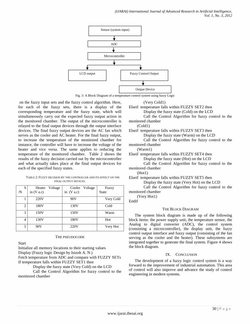
(IJARAI) International Journal of Advanced Research in Artificial Intelligence,
Vol. 1, No. 3, 2012
30 | P a g e
www.ijarai.thesai.org
Fig. 3: A Block Diagram of a temperature control system using fuzzy Logic
on the fuzzy input sets and the fuzzy control algorithm. Here,
for each of the fuzzy sets, there is a display of the
corresponding temperature and the fuzzy state, which will
simultaneously carry out the expected fuzzy output action in
the monitored chamber. The output of the microcontroller is
relayed to the final output devices through the output interface
devices. The final fuzzy output devices are the AC fan which
serves as the cooler and AC heater. For the final fuzzy output,
to increase the temperature of the monitored chamber for
instance, the controller will have to increase the voltage of the
heater and vice versa. The same applies to reducing the
temperature of the monitored chamber. Table 2 shows the
results of the fuzzy decision carried out by the microcontroller
and what actually takes place at the final output devices for
each of the specified fuzzy states.
TABLE 2: FUZZY DECISION BY THE CONTROLLER AND ITS EFFECT ON THE
FINAL OUTPUT DEVICES.
S
/N
Heater Voltage
in (V a.c)
Cooler Voltage
in (V a.c)
Fuzzy
State
1 220V 90V Very Cold
2 180V 130V Cold
3 150V 150V Warm
4 130V 180V Hot
5 90V 220V Very Hot
THE PSEUDOCODE
Start
Initialize all memory locations to their starting values
Display (Fuzzy logic Design by Isizoh A. N.)
Fetch temperature from ADC and compare with FUZZY SETs
If temperature falls within FUZZY SET1 then
Display the fuzzy state (Very Cold) on the LCD
Call the Control Algorithm for fuzzy control to the
monitored chamber
(Very Cold1)
Elseif temperature falls within FUZZY SET2 then
Display the fuzzy state (Cold) on the LCD
Call the Control Algorithm for fuzzy control to the
monitored chamber
(Cold1)
Elseif temperature falls within FUZZY SET3 then
Display the fuzzy state (Warm) on the LCD
Call the Control Algorithm for fuzzy control to the
monitored chamber
(Warm1)
Elseif temperature falls within FUZZY SET4 then
Display the fuzzy state (Hot) on the LCD
Call the Control Algorithm for fuzzy control to the
monitored chamber
(Hot1)
Elseif temperature falls within FUZZY SET5 then
Display the fuzzy state (Very Hot) on the LCD
Call the Control Algorithm for fuzzy control to the
monitored chamber
(Very Hot1)
Endif
THE BLOCK DIAGRAM
The system block diagram is made up of the following block items: the power supply unit, the temperature sensor, the Analog to digital converter (ADC), the control system (consisting a microcontroller), the display unit, the fuzzy control output interface and fuzzy output (consisting of the fan serving as the cooler and the heater). These subsystems are integrated together to generate the final system. Figure 4 shows the block diagram.
IX. CONCLUSION
The development of a fuzzy logic control system is a way forward to the improvement of industrial automation. This area of control will also improve and advance the study of control engineering in modern systems.
Sensor (system input)
ADC
Microcontroller
Fuzzy Control Output LCD output
Output Device

(IJARAI) International Journal of Advanced Research in Artificial Intelligence,
Vol. 1, No. 3, 2012
31 | P a g e
www.ijarai.thesai.org
REFERENCES
[1] Okorie F.C, “Fuzzy Logic Systems”, Jet Publishers Ltd, Lagos, 2008.
[2] Willam C.P, Fuzzy Logic and Real Time Applications”, New Generation Publishers, Ibadan, Nigeria, 2009.
[3] Lewis A.P., “Optimal Fuzzy Logic Control Technique”, Whitecap Publishing Co., Lagos, Nigeria, 2009.
[4] Francis T.C., “Solutions to Fuzzy Logic Controls”, Septon M. Publishers, London, 2010.
[5] Douglas V.H., “Microcontrollers and Interfacing: Programming Hardware” McGraw Hill Inc, New York, 2008.
[6] Schuster A., “Microcontroller Principles and Applications”, Maxon Press Ltd, Rochester, 2008.
[7] Peters Andrew, “Real Time Controls”, Jones Communications, Ikeja, Lagos Nigeria, 2008.
[8] Dogan Ibrahim, “Microcontroller-Based Temperature Monitoring and Control”, Elsevier Science & Technology Book, Maryland, USA, 2002.
Power Supply Unit
(P.S.U)
Control System ( Microcontroller)
Display Unit (LCD)
Analog to Digital Converter Temperature
Sensor
(lm35) chip
Fuzzy Logic Control Output
Interface Fuzzy logic final output
device
(Temperature
Monitored chamber)
Fig 4: The Block diagram of the fuzzy logic control system

(IJARAI) International Journal of Advanced Research in Artificial Intelligence,
Vol. 1, No. 3, 2012
32 | P a g e
www.ijarai.thesai.org
A New Genetic Algorithm Based Lane-By-Pass
Approach for Smooth Traffic Flow on Road
Networks
Shailendra Tahilyani
Department of Electronics & Communication
Babu Banarasi Das University
Lucknow, India
Manuj Darbari and Praveen Kumar Shukla
Department of Computer Science & Engineering
Babu Banarasi Das University
Lucknow, India
Abstract— Traffic congestion in urban areas is a very critical
problem and increasing day-by-day due to increment in number
of vehicles and un-expandable traffic infrastructure. Several
intelligent control systems have been developed to deal with this
issue. In this paper, a new lane bypass algorithm has been
developed for route diversion resulting in smooth traffic flow on
the urban road networks. Genetic algorithms are utilized for the
parameter optimization in this approach. Finally, the results of
the proposed approach are found satisfactory.
Keywords- Genetic Algorithms, Fuzzy Logic, Neural Network,
Activity Theory.
I. INTRODUCTION
Urban Road traffic congestion [1] is a situation that is characterized by high number of vehicles on a road that leads to low speed and longer time taken for a journey. Population growth and exponential growth in number of vehicles have increased the problem of congestion on the country’s freeways and highways. Traffic congestion can be classified in two types recurring and non-recurring [2]. Recurring congestion is associated with expected delays, resulting from large number of vehicles at the same time (during peak commuting) at the same place (at busy intersection).Non-recurring congestion is associated with unpredictable delays that are created by spontaneous traffic incidents, such as accidents.
The development of control systems to deal with the congestion for smooth flow of Traffic in urban areas is a critical research issue. Several conventional methods [3-10] have been applied to reduce the problem of traffic congestion. Some of these are, road pricing, supporting the green traffic, parking enforcement, fuel levies, expansion of existing road network, elimination of roundabout and many more. But due to non-linear and unpredictable nature of the traffic movement and the high cost associated with the expansion of existing infrastructure of road networks, the conventional methods are not found very suitable.
Meanwhile, the technology has been integrated to develop some intelligent control systems to deal with the traffic congestion issues, more specifically in urban areas.
Different approaches have been integrated to model and simulate the real time traffic control system, like activity
theory [11-13], neural network [14-16], fuzzy logic [17-18], petri nets [19-20], genetic algorithms [21] and their hybrid approaches.
This paper has been divided into 4 sections. In section II, the basic concepts of the proposed system are described. The new proposed algorithm is discussed in Section III. The results analysis of the proposed systems is carried out in the Section IV. Section V is the conclusion and future scope of the proposed approach.
II. BASIC CONCEPTS FOR PROPOSED SYSTEM
The Road Network in the urban areas can be considered as a graph. In this graph, edges are classified into two categories: 1. Major Lanes, 2. Minor Sublanes. During peak hours of the traffic movement, the Minor Sublanes can be utilized to overcome any situation of traffic congestion on the major roads of the road network. The prediction of the traffic congestion and transfer of this information is carried out by the proposed algorithm. The information passing and presentation are done by the VMS (Variable Message Sign Board).
A sample road network in the Lucknow City is presented in Fig. 1.
Fig. 1 A Sample Road Network in the Lucknow City
The major activities in the proposed approach are identified as follows:
1) Identification of Route Network in the city, showing the
relationship between all the roads (routes).

(IJARAI) International Journal of Advanced Research in Artificial Intelligence,
Vol. 1, No. 3, 2012
33 | P a g e
www.ijarai.thesai.org
2) Identification of Traffic Jams and then identification of
alternative minor sub lane route information.
3) Coordination among all the decision (alternative traffic
routes) to ensure the smooth traffic flow from source to
destination. The road network is described graph with links Zz and
junctions Jj . For each signalized junction j, we define the
sets of incoming Ij and outgoing Oj links. The signal control plan of junction j is based on a fixed number of stages that belong to the set, whereas v2 denotes the set of stages where link 2 has right of way. Finally the saturation flow S2 of link
Zz and the turning movement rates tx,y, where iIx and
jOy ,are assumed to be known and constant.
By definition, the constraint
CLgnFi
nmn
, holds at junction n, where mng , is the
green time of state m at junction n and Ln is the total lost time at junction n. It follows the constraints,
nmnnm Fmgg min,,,
Consider the following N Dimensional road network for result analysis in this paper.
Fig. 2 N Dimensional Road Network
A, B, C…….,I are the junctions(Places) at the traffic road network( and connected by road connectives(Transition). The modeling of each junction will be done as discussed in the first section. The phases and movements will be done in the same way.
The proposed approach for route diversion and selection is based on the Genetic Algorithm, an evolutionary techniques for the purpose of optimization in complex ill-defined search spaces. Genetic Algorithms are search and optimization techniques based on Darwinian’s principle of Natural Selection. The basic idea behind the natural selection is “select the best, discard the rest”. The optimization strategies by
genetic algorithms are implemented by simulating evolution of species through the natural selection.
The fundamental technique behind the GA includes the three steps: 1. Evaluation of individual fitness, 2. Formation of gene pool, intermediate population through the selection mechanism, 3. Recombination through the crossover and mutation operators.
The working of the GA can be well expressed by the
following data flow diagram, clearly.
Fig. 3 Working of Genetic Algorithms
III. PROPOSED SYSTEM
The problem is identified and mathematically formulated as:
Set of junctions J = (A, B, C, D, E, F, G, H, I)
Set of connectives E = (e1, e2, e3 ……….e23)
Set of Minor Sublanes M= (m1, m2, m3, m4)
The traffic flow will be decided by the set of connectives from source to destination. Few of the connectives are the bypass connectives that are used by transfer office by pass when the major connectives are full with traffic jam.
In this approach, the VMS technology is used. The commuters will find the signal for route diversion before one crossing through minor sub lane generation if there is any traffic jam at the next crossing. But overall it is also considered that the path from source to destination should be as minimum as possible.
To deal with this problem, the sensors will be placed at each junction for intimating the traffic jam to the previous junction by VMS.
Let the commuter is travelling from station A to I as shown Fig. 4. Now consider the situation, where the commuter

(IJARAI) International Journal of Advanced Research in Artificial Intelligence,
Vol. 1, No. 3, 2012
34 | P a g e
www.ijarai.thesai.org
identifies traffic congestion at junction G through VMS where he is on the route e4 at junction D. Now to deal with this situation the control system would generate the signal for route diversion through minor lane by pass and the commuter would get the signal to choose the route m1 and m4 to reach his destination.
The procedure of route diversion should be integrated with the approach traffic phase and movement decision approaches.
A. Algorithm ROUTE DIVERSION through minor sub-lane
For the route diversion the proposed algorithm is as follows:
ROUTE DIVERSION (αVMS, αMVMS )
1. Start
2. Generate αVMS for each junction at different intervals
of time.
αVMS = Traffic Flow / Mean Velocity
The value of Traffic Flow will be estimated by the
Sensors and Mean Velocity is calculated at different time
intervals.
Repeat steps 3 to 5 until the desired destination,
3. Collect the values of αVMS (update them on time
intervals) for all junctions in different paths from a
specified source to destination, at a control centre.
4. Generate the maximum value of αVMS from which the
traffic congestion will start and it is denoted by
αMVMS.
5. Apply minimization function Fmin on the values of
αVMS to get the next node, iteratively.
6. If Fmin (αVMS, αMVMS)≥ αVMS
then
Send the signal to previous junction’s VMS for route
diversion, if the selected junction is different from the
regular path,
otherwise
Follow the main route decided previously.
7. End.
B. GA ROUTE Diversion Algorithm
This route diversion process can be seen as an optimization problem and its extended version can be produced using genetic algorithm. This proposal is as follows:
GA- ROUTE DIVERSION (αVMS, αMVMS)
{
Initialize all the paths as first population
(e1, e2, ……………., en)
Evaluate the fitness of the each path as per the
function
Fmin (αVMS, αMVMS)
Set the termination criteria
Fmin (αVMS, αMVMS)≥ αVMS
while the termination criteria is satisfied
{
Select the most optimized path
Crossover (Various combinations of paths)
Mutation (Change a particular path in the
route)
Evaluate the new population
}
}
IV. RESULT ANALYSIS
The two cases are considered here for result analysis. Let the source station is A and destination station is I.
The selected route by commuter is (A, B, C, F, I). Now according to the space capacity of the junction, αMVMS =9.5 (for junction C). Here, TABLE I shows the traffic flow, mean velocity and calculated values of αVMS. at different time intervals in a day.
TABLE I : TRAFFIC FLOW & MEAN VELOCITY [JUNCTION C]
Time Traffic Flow Mean velocity (km/h) αVMS
7:00 AM 10 60 0.16
7:30 AM 20 40 0.50
8:00 AM 40 30 1.33
8:30 AM 60 25 2.40
9:00 AM 100 20 5.00
9:30 AM 150 15 10.00
10:00AM 200 10 20.00
10:30 AM 250 05 50.00
Case 1
At time 9:00 AM,
Fmin (αVMS , αMVMS) =Fmin (5, 9.5) < αVMS
Hence according to the algorithm, no diversion is required through the minor sub lane by- pass. This case is shown in Figure 4.
Fig. 4 Case 1
Case 2 At time 9:30 AM,
Fmin (αVMS , αMVMS) =Fmin (10, 9.5) > αVMS Hence according to the algorithm, the minor lane by pass
would be generated and the commuter will get the signal to divert the route at minor lane m2. This case is shown in Figure 5.
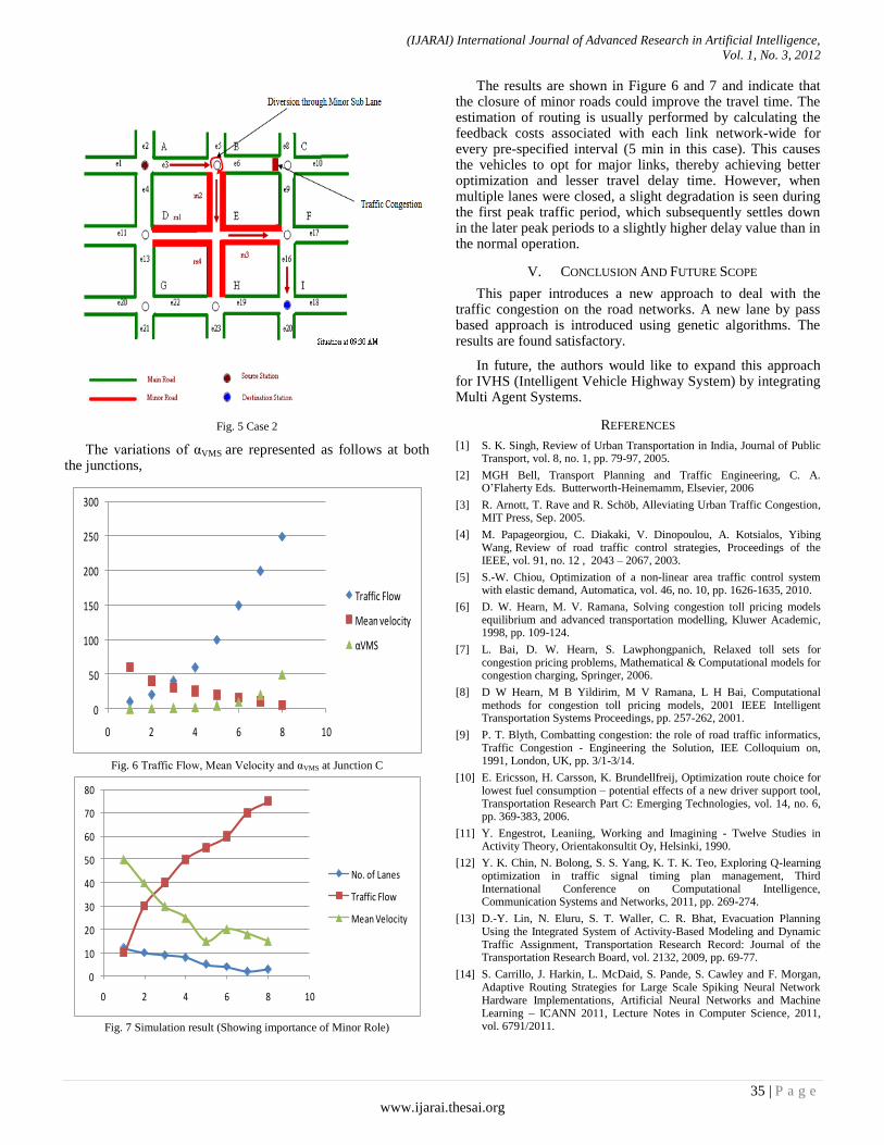
(IJARAI) International Journal of Advanced Research in Artificial Intelligence,
Vol. 1, No. 3, 2012
35 | P a g e
www.ijarai.thesai.org
Fig. 5 Case 2
The variations of αVMS are represented as follows at both the junctions,
0
50
100
150
200
250
300
0 2 4 6 8 10
Traffic Flow
Mean velocity
αVMS
Fig. 6 Traffic Flow, Mean Velocity and αVMS at Junction C
0
10
20
30
40
50
60
70
80
0 2 4 6 8 10
No. of Lanes
Traffic Flow
Mean Velocity
Fig. 7 Simulation result (Showing importance of Minor Role)
The results are shown in Figure 6 and 7 and indicate that the closure of minor roads could improve the travel time. The estimation of routing is usually performed by calculating the feedback costs associated with each link network-wide for every pre-specified interval (5 min in this case). This causes the vehicles to opt for major links, thereby achieving better optimization and lesser travel delay time. However, when multiple lanes were closed, a slight degradation is seen during the first peak traffic period, which subsequently settles down in the later peak periods to a slightly higher delay value than in the normal operation.
V. CONCLUSION AND FUTURE SCOPE
This paper introduces a new approach to deal with the traffic congestion on the road networks. A new lane by pass based approach is introduced using genetic algorithms. The results are found satisfactory.
In future, the authors would like to expand this approach for IVHS (Intelligent Vehicle Highway System) by integrating Multi Agent Systems.
REFERENCES
[1] S. K. Singh, Review of Urban Transportation in India, Journal of Public Transport, vol. 8, no. 1, pp. 79-97, 2005.
[2] MGH Bell, Transport Planning and Traffic Engineering, C. A. O’Flaherty Eds. Butterworth-Heinemamm, Elsevier, 2006
[3] R. Arnott, T. Rave and R. Schöb, Alleviating Urban Traffic Congestion, MIT Press, Sep. 2005.
[4] M. Papageorgiou, C. Diakaki, V. Dinopoulou, A. Kotsialos, Yibing Wang, Review of road traffic control strategies, Proceedings of the IEEE, vol. 91, no. 12 , 2043 – 2067, 2003.
[5] S.-W. Chiou, Optimization of a non-linear area traffic control system with elastic demand, Automatica, vol. 46, no. 10, pp. 1626-1635, 2010.
[6] D. W. Hearn, M. V. Ramana, Solving congestion toll pricing models equilibrium and advanced transportation modelling, Kluwer Academic, 1998, pp. 109-124.
[7] L. Bai, D. W. Hearn, S. Lawphongpanich, Relaxed toll sets for congestion pricing problems, Mathematical & Computational models for congestion charging, Springer, 2006.
[8] D W Hearn, M B Yildirim, M V Ramana, L H Bai, Computational methods for congestion toll pricing models, 2001 IEEE Intelligent Transportation Systems Proceedings, pp. 257-262, 2001.
[9] P. T. Blyth, Combatting congestion: the role of road traffic informatics, Traffic Congestion - Engineering the Solution, IEE Colloquium on, 1991, London, UK, pp. 3/1-3/14.
[10] E. Ericsson, H. Carsson, K. Brundellfreij, Optimization route choice for lowest fuel consumption – potential effects of a new driver support tool, Transportation Research Part C: Emerging Technologies, vol. 14, no. 6, pp. 369-383, 2006.
[11] Y. Engestrot, Leaniing, Working and Imagining - Twelve Studies in Activity Theory, Orientakonsultit Oy, Helsinki, 1990.
[12] Y. K. Chin, N. Bolong, S. S. Yang, K. T. K. Teo, Exploring Q-learning optimization in traffic signal timing plan management, Third International Conference on Computational Intelligence, Communication Systems and Networks, 2011, pp. 269-274.
[13] D.-Y. Lin, N. Eluru, S. T. Waller, C. R. Bhat, Evacuation Planning Using the Integrated System of Activity-Based Modeling and Dynamic Traffic Assignment, Transportation Research Record: Journal of the Transportation Research Board, vol. 2132, 2009, pp. 69-77.
[14] S. Carrillo, J. Harkin, L. McDaid, S. Pande, S. Cawley and F. Morgan, Adaptive Routing Strategies for Large Scale Spiking Neural Network Hardware Implementations, Artificial Neural Networks and Machine Learning – ICANN 2011, Lecture Notes in Computer Science, 2011, vol. 6791/2011.

(IJARAI) International Journal of Advanced Research in Artificial Intelligence,
Vol. 1, No. 3, 2012
36 | P a g e
www.ijarai.thesai.org
[15] A. Nagare, S. Bhatia,Traffic Flow Control using Neural Network, International Journal of Applied Information Systems (IJAIS) , vol. 1, no. 2, January 2012 .
[16] S. Carrillo, J. Harkin, L. McDaid, S. Pande, S. Cawley, B. McGinley, F. Morgan, Advancing interconnect density for spiking neural network hardware implementations using traffic-aware adaptive network-on-chip routers, Neural Networks, vol. 33, Sept. 2012, pp. 42–57.
[17] S. Mehan, V. Sharma, Development of traffic light control system based on Fuzzy Logic, ACAI '11 Proceedings of the International Conference on Advances in Computing and Artificial Intelligence, 2011.
[18] V. P. Vijayan, B. Paul, Multi Objective Traffic Prediction Using Type-2 Fuzzy Logic and Ambient Intelligence, Advances in Computer
Engineering (ACE), 2010 International Conference on, pp. 309-311, 2010.
[19] G. F. List, M. Setin, Modeling traffic signal control using petri nets, IEEE Transactions on Intelligent Transportation Systems, vol. 5, no. 3, Sept. 2004.
[20] H. Wang, Modeling and analysis of traffic signal systems using Petri nets, Ph.D. dissertation, Dept. Civil Eng., Rensselaer Polytechnic Inst., Troy, NY, 1992.
[21] J. J. Sanchez-Medina, Traffic Signal Optimization in “La Almozara” District in Saragossa Under Congestion Conditions, Using Genetic Algorithms, Traffic Microsimulation, and Cluster Computing, IEEE Transactions on Intelligent Transportation Systems, vol. 11, no. 1, pp. 132 – 141, 2010.

(IJARAI) International Journal of Advanced Research in Artificial Intelligence,
Vol. 1, No. 3, 2012
37 | P a g e
www.ijarai.thesai.org
Leaf Image Segmentation Based On the Combination
of Wavelet Transform and K Means Clustering
N.Valliammal
Assistant Professor, Department of Computer Science,
Avinashilingam Institute of Home Science and Higher
Education for Women
Coimbatore, Tamilnadu, India.
Dr.S.N.Geethalakshmi
Associate Professor, Department of Computer Science,
Avinashilingam Institute of Home Science and Higher
Education for Women
Coimbatore, Tamilnadu, India.
Abstract— This paper focuses on Discrete Wavelet Transform
(DWT) associated with the K means clustering for efficient plant
leaf image segmentation. Segmentation is a basic pre-processing
task in many image processing applications and essential to
separate plant leafs from the background. Locating and
segmenting plants from the background in an automated way is a
common challenge in the analysis of plant images. Image
segmentation is typically used to locate objects and boundaries
(lines, curves, etc.) in images. Image segmentation is a
fundamental task in agriculture computer graphics vision.
Although many methods are proposed, it is still difficult to
accurately segment an arbitrary image by one particular method.
In recent years, more and more attention has been paid to
combine segmentation algorithms and information from multiple
feature spaces (e.g. color, texture, and pattern) in order to
improve segmentation results .The performance of the
segmentation is analyzed by Jaccard, dice, variation of index and
global consistency error method. The proposed approach is
verified with real time plant leaf data base. The results of
proposed approach gives better convergence when compare to
existing segmentation method.
Keywords- Image segmentation; Wavelet Transform; Haar
Wavelet; K means clustering algorithm.
I. INTRODUCTION
Image segmentation is an essential step in many advanced techniques that covers multi-dimensional image processing and its applications. Digital Plant leaf analysis occupies an important place in many tasks such as in medical and agricultural field. Image segmentation techniques [6] are mostly used in plant leaf image processing field for detecting structures such as viens nodes, curvature and color of leaf detection. There are many approaches to image segmentation such as classifications, edges, or regions (Beaulieu and Touzi, 2004). Several techniques have been proposed for image segmentation using region growing (see Deng and Manjunath, 2001), graph cuts (see Boykov and Funka-Leam, 2006; Rother et al.2004), normalized cuts (see Shi and Malik, 2000), relaxation-based techniques (see Rosen-field et al., 1976), neural network based approaches (see Shan et al., 2005), methods based on fuzzy theory (see Hall, 1992), level sets (see Vese and Chan, 2002), and Markov random fields (see Schwartz and Pedrini, 2007). Comprehensive reviews of image segmentation techniques are described by Pal and Pal (1993) and Cremers (2007).
This paper describes the technique of wavelet transform use for features extraction associated with individual image pixels and combining this method with application of the k means clustering technique. For the image decomposition and feature extraction Haar transform has been applied as a basic tool used in the wavelet transform. A specific part of the paper is explained about the decomposition and reconstruction matrices. The method described is used for description of the whole system enabling perfect image reconstruction. The proposed algorithm of the Haar wavelet image decomposition includes image feature based segmentation with k means clustering algorithm. Individual methods have been verified for standard images and then applied for processing of selected real time plant leaf images.
In this paper, a proposed approach that makes use of wavelets and K means clustering is applied for leaf images. Through wavelets high pass image is extracted and to enhance edge details further decomposition is applied, which provides fine enhanced edge details with wavelet features like energy and entropy. The wavelet features and the k means are combined in our method to give better accuracy results.
The paper is organized as follows a brief literature survey is discussed in Section 2. The details of proposed approach is presented in Section 3 while Section 4 demonstrates the results of the proposed method. The conclusion is given in Section 5.
II. THE REVIEW OF WAVELET TRANSFORM
The wavelet transform (WT), a linear integral transform that maps L2 (R)→L2 (R
2 ) , has emerged over the last two
decades as a powerful new theoretical framework for the analysis and decomposition of signals and images at multi-resolutions [3].
Moreover, due to its locations in both time/space and in frequency, this transform is to completely differ from Fourier transform [4,5]. The region-based systems which use wavelet transform are classified into the following three categories according to the space units in which feature values for segmentation are calculated;
• A hierarchical block
• A moving window
• A pixel

(IJARAI) International Journal of Advanced Research in Artificial Intelligence,
Vol. 1, No. 3, 2012
38 | P a g e
www.ijarai.thesai.org
In [6], an image is segmented into hierarchical blocks by generating a quad tree. Then, for each block, statistics of wavelet coefficients (mean absolute value and variance) are computed in each subband, and used as features. The quad tree segmentation matches the multi level resolution analysis, and the features for each block can be obtained by applying wavelet transform only once to a whole image. Therefore, the computational cost is low. However, the method has low flexibility in the shapes of segmented regions. In [7], the method of nona-tree is proposed, instead of quad tree. Quad tree representation enables more flexible image segmentations. However, the computational cost is high, since the method requires wavelet transform for each block [21][22][23].
A. Haar Wavelets in Image Decomposition
Wavelets are functions generated from a single function by its dilations and translations. The Haar transform forms the simplest compression process of this kind. In 1-dimension, the corresponding algorithm [4] transforms a 2-element vector [x(1), x(2)]T into [y(1), y(2)]T by relation:
(1)
is an orthonormal matrix as its rows are orthogonal to each other (their dot products are zero). Therefore T−1 = TT and it is possible [4] to recover x from y by relation
(2) In 2-dimensions x and y become 2 × 2 matrices. at first
transform the columns of x, by pre-multiplying by T, and then the rows of the result by post-multiplying [4] by TT to find
y = TxTT and in the next step x = TT yT (3) To show more clearly what is happening in a specific
matrix is x of the form is applied
(4)
These operations correspond to the following filtering processes:
Top left: 2-D lowpass filter (Lo-Lo).
Top right: horizontal highpass and vertical lowpass filter
(Hi-L0)
Lower left: horizontal lowpass and vertical highpass filter
(L0-Hi)
Lower right: 2-D highpass filter (Hi-Hi).
To apply this transform to a complete image, the pixels are grouped into 2 × 2 blocks and apply Eq. (3) to each block. To
view the result, all the top left components in of the 2 × 2 blocks in y were grouped together to form the top left subimage and the same for the components in the other three positions. It is clear from Fig. 1(b) that the most of the energy is contained in the top left (Lo-Lo) subimage and the least energy is in the lower right (Hi-Hi) subimage. The top right (Hi-Lo) and the lower left (Lo-Hi) subimage contains [4] the edges.
Following subsections describe algorithms of image segmentation using wavelet transform with resulting images presented in Fig. 1.
B. Image Features Extraction
Texture is characterized by the spatial distribution of gray levels in a neighborhood. An image region has a constant texture if a set of its local properties in that region is constant, slowly changing or approximately periodic. Texture analysis is one of the most important techniques used in analysis.
There are three primary issues in texture analysis: classification, segmentation and shape recovery from texture. Analysis of texture [1] requires the identification of proper attributes or features that differentiate the textures of the image. In this paper, texture segmentation is carried out by comparing co-occurrence matrix features. Contrast and Energy of size N × N is derived from discrete wavelet transform overlapping but adjacent subimages Cij of size 4 × 4 lays horizontally and vertically. The algorithm of image features extraction involves
1) Decomposition, using one level DWT with the Haar
transform, of each subimage Ci,j of size 4 × 4 taken from the
top left corner
2) Computation of the co-occurrence matrix features
energy and contrast given in Eqs (3) and (4) from the detail
coefficients, obtained from each subimage Ci,j
3) Forming new feature matrices
C. Circular Averaging Filtering
In the image with the segmented band obtained after differences could appear with artifacts or spurious spots. Within the same region where the high differences of features values appear, the spots and noise were formed. These spurious elements were removed by applying a circular averaging filter. First the filter with suitable radius was created and then applied for a segmented image to minimize and denoise the image.
D. Thresholding and Skeletonizing
The processed image is then thresholded using global image threshold with Otsu’s method [6] when a black and white image is obtained. The appearance of thick boundaries has to be thinned on the line for one pixel thickness. To process these specific morphology operations were used.
At first operation ’clean’ removes isolated pixels - individual 1’s that are surrounded by 0’s.
The second operation ’skel’ removes pixels on the boundaries of objects but does not allow objects to break apart. The remaining pixels make up the image skeleton.

(IJARAI) International Journal of Advanced Research in Artificial Intelligence,
Vol. 1, No. 3, 2012
39 | P a g e
www.ijarai.thesai.org
Figure 1 Proposed Methodology for Plant Leaf Image Segmentation
III. K MEANS CLUSTERING
Clustering is a process of organizing the objects into groups based on its attributes. A cluster is therefore a collection of objects which are “similar” between them and are “dissimilar” to the objects belonging to other clusters. An image can be grouped based on keyword (metadata) or its content (description).
In keyword based clustering, a keyword is a form of font which describes about the image keyword of an image refers to its different features. The similar featured images are grouped to form a cluster by assigning value to each feature.
In content based clustering [10], [11], [20] , [24],[25] a content refers to shapes, textures or any other information that can be inherited from the image itself. The tools, techniques and algorithms that are used originate from fields such as statistics, pattern recognition, signal processing etc. Clustering based on the optimization of an overall measure is a fundamental approach explored since the early days of pattern recognition.
The most popular method used efficiently for pattern recognition is K-means clustering.
In K-means clustering a centroid vector is computed for every cluster. The centroid must be chosen such that it should minimize the total distance within the clusters.
Both supervised and unsupervised clustering techniques are used in image segmentation. In supervised clustering method, grouping is done according to user feedback. In
unsupervised clustering, the images with high features may be very different in terms of semantics [16].
In K-means algorithm data vectors are grouped into predefined number of clusters [12][13]. At the beginning the centroids of the predefined clusters are initialized randomly. The dimensions of the centroids are same as the dimension of the data vectors. Each pixel is assigned to the cluster based on the closeness of the pixel [14], which is determined by the Euclidian distance measure. After all the pixels are clustered, the mean of each cluster is recalculated. This process is repeated until no significant changes result for each cluster mean or for some fixed number of iterations.
A. Global K-Means Algorithm
According to Likas [8] the global k-means clustering algorithm does not depend upon the initial parameter values and utilize the k-means algorithm as a local search procedure that constitutes a deterministic global optimization method. This technique proceed in an incremental way of attempting to optimally include one new cluster center at each stage instead of randomly selecting starting value for all clusters [17][18]. More particularly, to solve a clustering problem with k clusters the method proceeds as follows.
Step 1: The algorithm begins with one cluster (k=1) and cluster center corresponds to the centroid of the data set X.
Step 2: Perform N executions of the k-means to find two cluster (k=2) after the initial positions of the cluster centers: For k=1, the first cluster center is constantly placed at the optimal position. The second center at execution n is placed at
Input Image
Level 3
Decomposition IDWT
3 Level
Detailed
Image
Denoising and
Thresholding
Segmentation by K
Means Clustering
Segmented
Enhanced Image
3 level decomposition

(IJARAI) International Journal of Advanced Research in Artificial Intelligence,
Vol. 1, No. 3, 2012
40 | P a g e
www.ijarai.thesai.org
the position of the data point xn (n-1,…..,N). The best solution is obtained after N executions of the k-means algorithm.
Step 3: For k-1 clustering problem, the final solution is denoted by (c1,c2,….,ck-1).
The algorithm performs N execution of the k-means algorithm with initial positions (c1, c2…... ck-1, xn), where n varies from 1 to N to find solution for k-clustering problem. The best solution obtained in this process is considered as the final solution.
IV. PROPOSED METHODOLOGY
Our proposed methodology is a five-step process, graphically illustrated in Fig. 1. All these steps are briefly depicted below:
1. Wavelet transform is applied to an input Plant Leaf image to obtain wavelet decomposed image resulting in twelve subbands. All these subbands represent approximation, horizontal, vertical and diagonal components in the form of coefficients, respectively. LL subband contains low level and the other three (LH, HL, HH) contain high level details.
2. Denoise the decomposed leaf image using average filter and Global thresholding .Otsu’s model is applied for separating the background and the shape of leaf is extracted.
3. Set approximation coefficients in LL equal to zero and apply inverse wavelet transform to obtain a high pass image from the remaining (horizontal, vertical and diagonal) subbands. We call the resultant image level-3 (L3) detail image.
4. Add L3 to the original image to get a sharpened image.
5. Apply the K means clustering algorithm, as given in step [3], to segment the images that partition the data set into an optimal number of clusters. Same data points belong to one cluster and different data points belong to different clusters.
This algorithm accounts for variability in cluster shapes, cluster densities and the number of data points in each of the subsets. This K means has a drawback that it cannot work well in case of noisy plant leaf images. Therefore, the combination of wavelet and K means provides better results as wavelets are robust to noise and this combination also helped to remove in homogeneity and artifacts produced in plant leaf imaging
6. The edge information is rectified using sobel edge detector and finally the enhanced image is obtained.
Discrete Wavelet Transform (DWT) is applied to plant leaf images because wavelets provide frequency information as well as time-space localization. In addition, their multi-resolution character enables to visualize image at various scales and orientations. The multi-resolution property provides information about various high frequency components at different levels of decomposition.
Over-decomposition should however be avoided, because as the decomposition levels increase, there is a great risk that lower frequencies become a part of detail components. This may restrict us to use only fewer level of decomposition because lower frequencies will become part of high pass
image and reduce effective detail in an image.
V. EXPERIMEBNTAL RESULTS AND ANALYSIS
The proposed approach to a large set of Plant Leaf images forms a standard database. The step-by-step process, after applying the proposed method, is shown in Fig. 3. The performance of the proposed segmented algorithm is checked with FCM segmentation algorithm using clustering performance parameter jaccard, dice, variation of index and global consistency error method.
The input image is decomposed by DWT at level-3 and it gives a detail image (Fig.b) by setting subband to zero, applying the average filter for denoising noisy pixel image and to extract the object global thresholding and thereafter applying inverse DWT. The resultant detail image is then added to the original input image to result in a sharpened image shown in (Fig. e).
For Level 3 decomposed image K means algorithm is applied as shown in (Fig. d). It can be seen that contours are not properly highlighted and edge information is missing in some places.
To preserve edge information, sobel edge detection mask is applied to fill edges in cluster segmented image and the result is shown in (Fig. f).
A. Jaccard
The Jaccard index, also known as the Jaccard similarity coefficient is a statistic used for comparing the similarity and diversity of sample sets. The Jaccard coefficient measures similarity between sample sets, and is defined as the size of the intersection divided by the size of the union of the sample sets:
B. Dice
Dice coefficient, is a similarity measured over sets:
It is identical to the Sørensen similarity index, and is occasionally referred to as the Sørensen-Dice coefficient.
C. Variation of Information (VOI)
The Variation of Information (VOI) metric defines the distance between two segmentations as the average conditional entropy of one segmentation given to the other, measures the amount of randomness in one segmentation which cannot be explained by the other [21]. Suppose there are two clustering (a division of a set into several subsets) X and Y where X = {X1, X2... Xk}, pi = | Xi | / n, n = Σk | Xi |. Then the variation of information between two clustering is:
VI(X; Y) = H(X) + H(Y) − 2I(X, Y)
Where, H(X) is entropy of X and I(X, Y) is mutual information between X and Y. The mutual information of two clustering is the loss of uncertainty of one clustering if the

(IJARAI) International Journal of Advanced Research in Artificial Intelligence,
Vol. 1, No. 3, 2012
41 | P a g e
www.ijarai.thesai.org
other is given. Thus, mutual information is positive and bounded by {H(X),H(Y)}_log2(n).
D. Global Consistency Error (GCE)
The Global Consistency Error (GCE) measures the extent to which one segmentation can be viewed as a refinement of the other [21]. Segmentations which are related are considered to be consistent, could represent the same image segmented at different scales. Segmentation is simply a division of the pixels of an image into sets. The segments are sets of pixels. If one segment is a proper subset of the other, then the pixel lies in an area of refinement, and the error should be zero. If there is no subset relationship, then the two regions overlap in an consistent manner. The formula for GCE is as follows:
GCE = 1/n.min E(s1,s2, pi), E(s2, s1, pi)
Where, segmentation error measure takes two segmentations S1 and S2 as input, and produces a real valued output in the range [0::1] where zero signifies no error. For a given pixel pi consider the segments in S1 and S2 that contain that pixel.
The figure 3 shows the image results for different stages in proposed methodology. The proposed methodology consists of five stages. The input image, wavelet level 3 decomposed image, denoising and thresholding and finally enhanced segmentation image is shown in figure 2. In table 1, the proposed methodology gives the suitable results on the basis of comparing the jaccard, dice, variation of index and global consistency error.
TABLE 1 PARAMETRIC EVALUATION FOR DIFFERENT SEGMENTATION ALGORITHM
Algorithm Jaccard Dice VOI GCE
FCM 0.9455 0.0167 0.872 0.563
Wavelet 0.9440 0.0113 0.631 0.452
K means 0.953 0.0142 0.825 0.713
Proposed method 0.9688 0.0091 0.544 0.412
Figure- 2 Graphical results for Different Segmentation Algorithm
FCM
Wavelet
K means
Proposed method

(IJARAI) International Journal of Advanced Research in Artificial Intelligence,
Vol. 1, No. 3, 2012
42 | P a g e
www.ijarai.thesai.org
Fig-a- Original Image Fig-b- 3 Level Decomposed Image
Fig-c- Noisy Pixel Image Fig-d-Denoised by Average Filter
Fig-e- Global Thresholding Fig-f- K means and Sobel Enhanced Image
Figure- 3 Image results for Different Stage in Proposed Methodology

(IJARAI) International Journal of Advanced Research in Artificial Intelligence,
Vol. 1, No. 3, 2012
43 | P a g e
www.ijarai.thesai.org
VI. CONCLUSION
This paper discussed on Discrete Wavelet Transform (DWT) associated with the K means clustering for efficient plant leaf image segmentation. The performance of the segmentation is analyzed by Jaccard, dice, variation of index and global consistency error method.
The proposed approach is verified with real time plant leaf data base. The results of the proposed approach give better convergence when compared to conventional segmentation method.
REFERENCE
[1] Juin-Der Lee, Hong-Ren Su, MR Image Segmentation Using a Power Transformation Approach, P.1-13, 2008.
[2] C. H. Chen, G. G. Lee, Image Segmentation Using Multiresolution Wavelet Analysis and Expectation-Maximization (EM) Algorithm for Digital Mammography,wiley,1997.
[3] Neelum Noreen, Khizar Hayat and Sajjad A. Madani, MRI Segmentation through Wavelets and Fuzzy C-Means, World Applied Sciences Journal 13 (Special Issue of Applied Math): p. 34-39, 2011.
[4] R. C. Dubes and A. K. Jain. Algorithms for Clustering Data.Prentice Hall, 1988.
[5] T. Zhang, R. Ramakrishnan, and M. Livny. BIRCH: An Efficient Data Clustering Method for very Large Databases. Proc. of the 1996 ACM SIGMOD Int’l Conf. on Management of Data, Montreal, Canada, pages 103–114, June 1996.
[6] 7. S. Thilagamani1 and N. Shanthi2, A Survey on Image Segmentation Through Clustering, International Journal of Research and Reviews in Information Sciences Vol. 1, No. 1, P.14-18March 2011.
[7] G.C. Tseng. Penalized and weighted k-means for clustering with scattered objects and prior information in high-througput biological data. Bioinformatics, Vol.23, No.17, P.2247–2255, 2007.
[8] Mrunalini R. Badnakhe and Prashant R. Deshmukh, An Application of K-Means Clustering and Artificial Intelligence in Pattern Recognition for Crop Diseases, proceeding of International Conference on Advancements in Information Technology With workshop of ICBMG 2011, P.134-139,2011.
[9] R.Srinivasa Perumal, R.Sujatha, Analysis of Colon Cancer Dataset using K-Means based
[10] Algorithms & See5 Algorithms, IJCST Vol. 2, No. 4, P.482-485, 2011.
[11] B.Sathya, R.Manavalan, Image Segmentation by Clustering Methods: Performance Analysis, International Journal of Computer Applications Volume 29– No.11, P.0975 – 8887, 2011.
[12] 12. M. Sesli1* and E. D. Yegenoglu2, Compare various combinations of similarity coefficients and clustering methods for Olea europaea sativa, Scientific Research and Essays Vol. 5, No.16, P. 2318-2326, 2010.
[13] 13. Byung-Gyu Kim, Jae-Ick Shim, Dong-Jo Park, Fast image segmentation based on multi- esolution analysis and wavelets, Pattern Recognition Letters 24, P. 2995–3006, 2003.
[14] 14. J J . Lewis, R J O Callaghan, S G Nikolov, D R Bull, Region-Based Image Fusion Using Complex Wavelets, Image Rochester NY , Vol. 8, No. 2, Publisher: Citeseer, Pages: 119-130,2007.
[15] 15. Gonzalez, R. C.; Woods, R. E. 2002. Digital Image Processing. Prentice Hall, Inc., Upper Saddle River, New Jersey.
[16] 16. Lj.Jovanov, A. Piˇzurica, and W. Philips, “Wavelet based joint denoising of depth and luminance images,” in 3D TV conference, (Kos Island, Greece), 2007.
[17] 17. P. Scheunders, “Wavelet thresholding of multivalued images,” IEEE Trans. Image Proc. 13, pp. 475– 483, 2004.
[18] 18. P. Scheunders and S. De Backer, “Wavelet denoising of multicomponent images, using a noise-free image,” in Proc. IEEE Internat. Conf. Image Proc. ICIP, 2006.
[19] 19. P. Jayamala K. Patil , Raj Kumar, Advances in Image Processing for Detection of plant diseases, Journal of Advanced Bioinformatics Applications and Research ISSN 0976-2604 Vol 2, N0. 2, June-2011, pp 135-141.
[20] zGurbinder kaur, Intensity based image Segmentation using Wavelet analysis and Clustering techniques, indian journal of computer science and engineering (ijcse), vol. 2 no. 3 jun-jul 20
[21] Mr. Viraj A. Gulhane, Dr. Ajay A. Gurjar, Detection of Diseases on Cotton Leaves and Its PossibleDiagnosisInternational Journal of Image Processing (IJIP),Vol.5 , No.5 , P.590-598, 2011.
[22] Nourhan M. Zayed (et.al), Wavelet Segmentation for Fetal Ultrasound Images, IEEE paper, 2010.
[23] Yui-Liang Chen (et.al), Color Image Segmentation Using Wavelet Transform Techniques, 16th IPPR Conference on ComputerVision, Graphics and Image Processing (CVGIP 2003), P.669-675, 2003.
[24] Gurpreet kaur and Himanshu Monga, Classification of Biological Species Based on Leaf Architecture–A review, IRACST - International Journal of Computer Science and Information Technology & Security (IJCSITS),Vol. 2, No.2, P.332-334, 2012.
[25] Jyotismita Chaki and Ranjan Parekh, Plant Leaf Recognition using Shape based Features and Neural Network classifiers, (IJACSA) International Journal of Advanced Computer Science and Applications, Vol. 2, No. 10, P.41-48,2011

(IJARAI) International Journal of Advanced Research in Artificial Intelligence,
Vol. 1, No. 3, 2012
44 | P a g e
www.ijarai.thesai.org
Poultry Diseases Warning System using Dempster-
Shafer Theory and Web Mapping
Andino Maseleno
Computer Science Program
Faculty of Science, Universiti Brunei Darussalam
Jalan Tungku Link, Gadong BE 1410, Brunei Darussalam
Md. Mahmud Hasan
Computer Science Program
Faculty of Science, Universiti Brunei Darussalam
Jalan Tungku Link, Gadong BE 1410, Brunei Darussalam
Abstract— In this research, the researcher built a Web Mapping
and Dempster-Shafer theory as an early warning system of
poultry diseases. Early warning is the provision of timely and
effective information, through identified institutions, that allows
individuals exposed to a hazard to take action to avoid or reduce
their risk and prepare for effective response. In this paper as an
example we use five symptoms as major symptoms which include
depression, combs, wattle, bluish face region,
swollen face region, narrowness of eyes, and balance disorders.
Research location is in the Lampung Province, South Sumatera.
The researcher’s reason to choose Lampung Province in South
Sumatera on the basis that has a high poultry population. Our
approach uses Dempster-Shafer theory to combine beliefs in
certain hypotheses under conditions of uncertainty and
ignorance, and allows quantitative measurement of the belief and
plausibility in our identification result. Web Mapping is also used
for displaying maps on a screen to visualize the result of the
identification process. The result reveal that Poultry Diseases
Warning System has successfully identified the existence of
poultry diseases and the maps can be displayed as the
visualization.
Keywords-poultry diseases; early warning system; Dempster-Shafer
theory, web mapping
I. INTRODUCTION
The demand for chicken meat has been increasing because
it has become cheaper relative to other meats The term poultry
refers to domesticated fowl raised for meat or eggs. The
poultry industry is dominated by the chicken companies,
development of poultry population and poultry industry is very
rapidly threatened by the presence of poultry disease. Disease
is defined as a departure from health, and includes any
condition that impairs normal body functions. Disease results
from a combination of indirect causes that reduce resistance or
predispose an animal to catching a disease, as well as the
direct causes that produce the disease. Avian influenza virus, which has been limited to poultry,
now has spread to migrating birds and has emerged in
mammals and among the human population. It presents a
distinct threat of a pandemic for which the World Health
Organization and other organizations are making preparations
[1]. In 2005, the World Health Assembly urged its Member
States to develop national preparedness plans for pandemic
influenza [2]. Developing countries face particular planning
and other challenges with pandemic preparedness as there may
be a higher death rate in developing countries compared with
more developed countries [3].
In this research, we were using chicken as research object
because chicken population has grown very fast in Lampung
Province at 2009, native chicken population around
11,234,890, broiler population around 15,879,617, layer
population around 3,327,847. Lampung Province has been
divided into 10 regencies, 204 districts and 2279 villages with
area of 3,528,835 hectare [4].
To overcome poultry diseases required an early warning
system of poultry diseases. International Strategy for Disaster
Reduction (ISDR) defines early warning as the provision of
timely and effective information, through identified
institutions, that allows individuals exposed to a hazard to take
action to avoid or reduce their risk and prepare for effective
response [5].. The remainder is organized as follows. The Web mapping
is briefly reviewed in Section 2. Section 3 details the proposed Dempster-Shafer Theory. Architecture of Poultry Diseases Warning System is detailed in Section 4. The experimental results are presented in Section 5, and final remarks are concluded in Section 6.
II. WEB MAPPING
Web mapping is the process of designing, implementing,
generating and delivering maps on the World Wide Web and
its product. While web mapping primarily deals with
technological issues, web cartography additionally studies
theoretic aspects: the use of web maps, the evaluation and
optimization of techniques and workflows, the usability of web
maps, social aspects, and more. Web Geographic Information
System (GIS) is similar to web mapping but with an emphasis
on analysis, processing of project specific geo data and
exploratory aspects [6].
The web mapping server is the engine behind the maps [7].
The mapping server or web mapping program needs to be
configured to communicate between the web server and
assemble data layers into an appropriate image. A map is not
possible without some sort of mapping information for display.
Mapping data is often referred to as spatial or geospatial data
and can be used in an array of desktop mapping programs or
web mapping servers. Mapping data in the Poultry Diseases

(IJARAI) International Journal of Advanced Research in Artificial Intelligence,
Vol. 1, No. 3, 2012
45 | P a g e
www.ijarai.thesai.org
Warning System uses spatial and non-spatial data in ArcView
format. Table 1 shows the data mapping.
TABLE I. DATA MAPPING
Data Type Data Name Description
Spatial Province
Regencies
District Desa
Spatial Data digitized on
screen with ArcView
Non-Spatial Province Table
Regency Table
District Table Village Table
Data tabulated into flat table
of which follow data spatial
III. DEMPSTER-SHAFER THEORY
The Dempster-Shafer theory was first introduced by
Dempster [8] and then extended by shafer [9], but the kind of
reasoning the theory uses can be found as far back as the
seventeenth century. This theory is actually an extension to
classic probabilistic uncertainty modeling. Whereas the
Bayesian theory requires probabilities for each question of
interest, belief functions allow us to base degrees of belief for
on question on probabilities for a related question. The
Dempster-Shafer (D-S) theory or the theory of belief functions
is a mathematical theory of evidence which can be interpreted
as a generalization of probability theory in which the elements
of the sample space to which nonzero probability mass is
attributed are not single points but sets. The sets that get
nonzero mass are called focal elements. The sum of these
probability masses is one, however, the basic difference
between D-S theory and traditional probability theory is that
the focal elements of a Dempster-Shafer structure may overlap
one another. The D-S theory also provides methods to
represent and combine weights of evidence.
m: 2Θ
→ [0,1] is called a basic probability assignment (bpa)
over Θ if it satisfies
m (Ø) = 0 and
(1)
From the basic probability assignment, the upper and lower
bounds of an interval can be defined. This interval contains the
precise probability of a set of interest and is bounded by two
nonadditive continuous measures called Belief (Bel) and
Plausibility (Pl). The lower bound for a set A, Bel(A) is
defined as the sum of all the basic probability assignments of
the proper subsets (B) of the set of interest (A) (B ⊆ A ).
Formally, for all sets A that are elements of the power set, A
∈ 2Θ
(2)
A function PL: 2Θ
→[0,1] is called a plausibility function
satisfying
(3)
The plausibility represents the upper bound for a set A, and
is the sum of all the basic probability assignments of the sets
(B) that intersect the set of interest (A) ( B∩A ≠φ ). The precise
probability P(A) of an event (in the classical sense) lies within
the lower and upper bounds of Belief and Plausibility,
respectively: Bel(A) ≤ P(A) ≤ PL(A) (4)
In terms of previous work using Dempster-Shafer theory to
estimate stand regeneration maps [10], [11]. Actually,
according to researchers knowledge, Dempster-Shafer theory
of evidence has never been used for built an early warning
system of poultry diseases fusion with Web Mapping.
The result is that Poultry Diseases Warning System
successfully identifying disease and displaying location to
visualize the result of identification process.
Symptoms:
1. Depression
2. Combs, wattle, bluish face region
3. Swollen face region
4. Narrowness of eyes
5. Balance disorder
A. Symptom 1
Depression is a symptom of Avian Influenza (AI),
Newcastle Disease (ND), Fowl Cholera (FC), Infectious
Bronchitis respiratory form (IBRespi), Infectious Bronchitis
reproduction form (IBRepro), and Swollen Head Syndrome
(SHS). The measures of uncertainty, taken collectively are
known in Dempster Shafer Theory terminology as a ``basic
probability assignment'' (bpa). Hence we have a bpa, say m1 of
0.7 given to the focal element {AI, ND, FC, IBRespi,
IBRepro, SHS} in example, m1({AI, ND, FC, IBRespi,
IBRepro, SHS}) = 0.7, since we know nothing about the
remaining probability it is allocated to the whole of the frame
of the discernment in example, m1({AI, ND, FC, IBRespi,
IBRepro, SHS}) = 0.3, so:
m1{AI, ND, FC, IBRespi, IBRepro, SHS} = 0.7
m1{Θ} = 1 - 0.7 = 0.3 (5)
B. Symptom 2
Combs, wattle, bluish face region are symptoms of Avian
Influenza with a bpa of 0.9, so that:
m2{AI} = 0.9
m2 {Θ} = 1 – 0.9 = 0.1 (6)
With the symptoms comb, wattle, bluish face region then
required to calculate the new bpa values for some
combinations (m3). Table 2 shows combination rules for m3.
TABLE II. COMBINATION OF SYMPTOM 1 AND SYMPTOM 2
We then calculate the combined of equation (5) and equation
(6) as shown in the equation (7).
m3 (AI) = 9.001
27.063.0

(IJARAI) International Journal of Advanced Research in Artificial Intelligence,
Vol. 1, No. 3, 2012
46 | P a g e
www.ijarai.thesai.org
m3 (AI, ND, FC, IBRespi, IBRepro, SHS) = 07.001
07.0
m3 (Θ) = 03.001
03.0
(7)
C. Symptom 3
Swollen face region is a symptom of Avian Influenza,
Newcastle Disease, Fowl Cholera with a bpa of 0.83, so that
m4 {AI, ND, FC} = 0.83
m4 (Θ) = 1 – 0.83= 0.17 (8)
With the symptom swollen face region then required to
calculate the new bpa values for each subset. Table 3 shows
combination rules for m5.
TABLE III. COMBINATION OF SYMPTOM 1, SYMPTOM 2, AND SYMPTOM 3
We then calculate the combined of equation (7) and equation
(8) as shown in the equation (9).
m5 (AI) =
m5 (AI, ND, FC) =
m5 (AI, ND, FC, IBRespi, IBRepro, SHS) =
m5 (Ө) =
(9)
D. Symptom 4
Narrowness of eyes is a symptom of Swollen Head
Syndrome with a bpa of 0.9, so that:
m6 (SHS) = 0.9
m6 (Θ) = 1 – 0.9 = 0.1 (10)
With the symptom narrowness of eyes then required to
calculate the new bpa values for each subset with bpa m7.
Table 4 shows combination rules for m7.
TABLE IV. COMBINATION OF SYMPTOM 1, SYMPTOM 2, SYMPTOM 3, AND
SYMPTOM 4
We then calculate the combined of equation (9) and equation
(10) as shown in the equation (11).
m7 (SHS) = 13270.0)0747.081.0(1
00459.001071.0
m7 (AI) = 78057.0)0747.081.0(1
09.0
m7 (AI, ND, FC) = 07199.0)0747.081.0(1
0083.0
m7 (AI, ND, FC, IBRespi, IBRepro, SHS) =
01032.0)0747.081.0(1
00119.0
m7 (Θ) = 00442.0)0747.081.0(1
00051.0
(11)
E. Symptom 5
Balance disorders is a symptom of Newcastle Diseases and
Swollen Head Syndrome with a bpa of 0.6, so that:
m8 {ND,SHS} = 0.6
m8 {Θ} = 1 - 0.6 = 0.4 (12)
With the symptom balance disorders will be required to
calculate the new bpa values for each subset with m9 bpa.
Table 5 shows combination rules for m9.
TABLE V. COMBINATION OF SYMPTOM 1, SYMPTOM 2, SYMPTOM 3, SYMPTOM
4, AND SYMPTOM 5
We then calculate the combined of equation (11) and equation
(12) as shown in the equation (13).
m9 (SHS) = 24960.046834.01
05308.007962.0
m9 (AI) = 58725.046834.01
31222.0
m9 (ND) = 08124.046834.01
04319.0
m9 (ND, SHS) = 01663.046834.01
00265.000619.0
m9 (AI, ND, FC) = 05417.046834.01
02880.0
m9 (AI, ND, FC, IBRespi, IBRepro, SHS) =
00777.046834.01
00413.0
083.001
0249.00581.0
0119.001
0119.0
0051.001
0051.0
9.001
153.0747.0

(IJARAI) International Journal of Advanced Research in Artificial Intelligence,
Vol. 1, No. 3, 2012
47 | P a g e
www.ijarai.thesai.org
m9 (Θ) = 00025.0061038.01
000232.0
(13)
The highest bpa value is the m9 (AI) that is equal to
0.58725 which means the possibility of a temporary diseases
with symptoms of depression, comb, wattle, bluish face
region, swollen region face, narrowness of eyes, and balance
disorders is the Avian influenza (H5N1).
IV. POULTRY DISEASES WARNING SYSTEM
Figure 1 shows architecture of Poultry Diseases Warning System which is fusion between the Dempster-Shafer theory and Web Map Application.
Figure 1. Architecture of Poultry Diseases Warning System
The development of Poultry Diseases Warning System to
begin with:
1. Preparation which includes installing and setting
programs.
2. Preparation of attributes data and spatial data that already
exist so it can be used by the program application.
3. Database design with MySQL. At this stage the databases
design regarding the depiction relationships between
entities using diagram of relationships between entities
(entity relationship diagrams).
4. Designing Web pages using PHP. This web page then
connected to the database and spatial attributes that have
been established to form a network of database.
5. Designing a Web-based applications used to access the
network database that has been formed. The relationship
between applications with network data base that has
shaped overall applications to manage information to be
displayed.
V. IMPLEMENTATION
Poultry Diseases Warning System is applying web
mapping technology using MapServer software. Map data
obtained from digitized by ArcView for creating and editing
dataset. The implementation process is done after design and
scope of the system have been analyzed. Writing map file
using Macromedia Dreamweaver. Macromedia Dreamweaver
for writing map file that later on as the main file from system
configuration and layout as well. Spatial and non spatial data
designed using ArcView. Each data is designed to
accommodate operation at the layer level, either single layer or
multi layer. The following will be shown the working process of expert
system in diagnosing a case. The consultation process begins with selecting the location and symptoms found on the list of symptoms. In the cases tested, a known symptoms are depression, comb, wattle, bluish-colored facade region, region of the face swollen, eyes narrowed and balance disorders. The consultation process can be seen in Figure 2 and Figure 3.
Figure 2. Selecting Region of Consultation
Figure 3. Symptoms Selection
In the case of depression, comb, wattle and region of the face
bluish, region of the face swollen, eyes narrowed and
lachrymal glands swollen. The result of consultation is avian
influenza with bpa value equal to 0.587275693312. Figure 4
and figure 5 are showed the result of consultation and the
region map of consultation result. Consultation result shows
that needs serious treatment because has basic probability
assignment more than 0.5.
Data Preparation, File Management, Application Execution
Menu, Hyperlinks, Map Display, Query Spasial, Diseases Identification, Location Identification
Map Database Map Dempster-ShaferDempster-Shafer
Database
Knowledge Base
Map Components
Dempster-Shafer Model
Web Server
Web Browser
Spatial Database
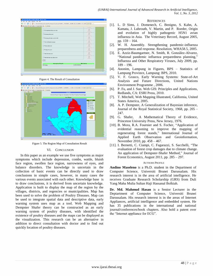
(IJARAI) International Journal of Advanced Research in Artificial Intelligence,
Vol. 1, No. 3, 2012
48 | P a g e
www.ijarai.thesai.org
Figure 4. The Result of Consultation
Figure 5. The Region Map of Consultation Result
VI. CONCLUSION
In this paper as an example we use five symptoms as major
symptoms which include depression, combs, wattle, bluish
face region, swollen face region, narrowness of eyes, and
balance disorders. The knowledge is uncertain in the
collection of basic events can be directly used to draw
conclusions in simple cases, however, in many cases the
various events associated with each other. Knowledge base is
to draw conclusions, it is derived from uncertain knowledge.
Application is built to display the map of the region by the
villages, districts, and regencies or municipalities. Map has
been used to solve the problem of Poultry Diseases. Map can
be used to integrate spatial data and descriptive data, early
warning system uses map as a tool. Web Mapping and
Dempster Shafer theory can be constructed as an early
warning system of poultry diseases, with identified the
existence of poultry diseases and the maps can be displayed as
the visualization. This research can be an alternative in
addition to direct consultation with doctor and to find out
quickly location of poultry diseases.
REFERENCES
[1]. L. D Sims, J. Domenech, C. Benigno, S. Kahn, A.
Kamata, J. Lubrouth, V. Martin, and P. Roeder, Origin
and evolution of highly pathogenic H5N1 avian
influenza in Asia. The Veterinary Record, August 2005,
pp. 159 – 164.
[2]. W. H. Assembly. Strengthening pandemic-influenza
preparedness and response. Resolution, WHA58.5, 2005.
[3]. E. Azziz-Baumgartner, N. Smith, R. González-Alvarez,
“National pandemic influenza preparedness planning,”
Influenza and Other Respiratory Viruses, July 2009, pp.
189 – 196.
[4]. Anonim, Lampung in Figures, BPS – Statistics of
Lampung Province, Lampung: BPS, 2010.
[5]. V. F. Grasco, Early Warning Systems: State-of-Art
Analysis and Future Directions, United Nations
Environment Programme , 2006.
[6]. P. Fu, and J. Sun. Web GIS: Principles and Applications,
Redlands, CA: ESRI Press, 2010.
[7]. T. Mitchell, Web Mapping Illustrated, California, United
States America, 2005.
[8]. A. P. Dempster, A Generalization of Bayesian inference,
Journal of the Royal Statistical Society, 1968, pp. 205 –
247.
[9]. G. Shafer, A Mathematical Theory of Evidence,
Princeton University Press, New Jersey, 1976.
[10]. B. Mora, R.A. Fournier and S. Focher, “Application of
evidential reasoning to improve the mapping of
regenerating forest stands,” International Journal of
Applied Earth Observation and Geoinformation,
November 2010, pp. 458 – 467.
[11]. I. Bernetti, C. Ciampi, C. Fagarazzi, S. Sacchelli, “The
evaluation of forest crop damages due to climate change.
An application of Dempster-Shafer Method,” Journal of
Forest Economics, August 2011, pp. 285 – 297.
AUTHORS PROFILE
Andino Maseleno is a Ph.D. student in the Department of
Computer Science, Universiti Brunei Darussalam. His
research interest is in the area of artificial intelligence. He
receives Graduate Research Scholarship (GRS) from Duli
Yang Maha Mulia Sultan Haji Hassanal Bolkiah.
Dr. Md. Mahmud Hasan is a Senior Lecturer in the
Deptartment of Computer Science, Universiti Brunei
Darussalam. His research interest is in the areas of Internet
Appliances, artificial intelligence and embedded system. He
has 35 publications in the international and national
journal/conferences/book chapters. Also hold a patent over
the “Internet appliance for ECG”.