Tc

Ma

b

a

ARRA

KMTISM

1

glsbmbb

att

1

SF

0h

Ecological Modelling 251 (2013) 173– 186

Contents lists available at SciVerse ScienceDirect

Ecological Modelling

jo ur n al homep ag e: www.elsev ier .com/ locate /eco lmodel

he Scaled Subspaces Method: A new trait-based approach to modelommunities of populations with largely inhomogeneous density

arco Castellania,∗, Selina Vågea, Espen Stranda,b, T. Frede Thingstada, Jarl Giskea

Department of Biology, University of Bergen, P.O. Box 7803, 5020 Bergen, NorwayInstitute of Marine Research, P.O. Box 1870 Nordnes, 5817 Bergen, Norway

r t i c l e i n f o

rticle history:eceived 19 July 2012eceived in revised form 3 December 2012ccepted 16 December 2012

eywords:odelling

rait-basedndividual-basedcaled subspacesicrobial food web

a b s t r a c t

We present a new individual-based approach to model populations of largely inhomogeneous densities.By monitoring different populations at a spatial scale which is inversely proportional to the maximumexpected concentration, the Scaled Subspaces Method solves the problem of demographic explosion ofthe most numerous species. It is intuitively similar to the experimental practice of changing the magni-fication of a microscope depending on the size-class of organisms inspected, and retains the possibilityfor uniform biological descriptions across scales. We use this method to simulate a pelagic microbialmixotrophic food web, where the most abundant species has population densities up to five orders ofmagnitude higher than the rarest species. The model generates biologically plausible and highly con-sistent predictions of biomass distribution across this density spectrum. Individual-based communitymodels are affected by the possibility of artificial extinctions. We discuss theoretically and confirmexperimentally this possibility, and show that this problem can be overcome through the use of large

populations, genetic mutations, and periodical random reintroduction of lost species or traits. We alsoshow that the proposed individual-based model produces the same solutions as a state-variable modelof the same ecological scenario. This indicates that the predictions of the two models are independentof implementation issues, and allows using them interchangeably according to convenience. Overall, thestudy proves the viability of the Scaled Subspaces Method, and provides useful insights on its functioningand parameterization.

© 2013 Elsevier B.V. All rights reserved.

. Introduction

Modelling biological systems often implies the representation ofroups of organisms of different size, density, and behaviour. Theiterature can be broadly divided into two main approaches: thetate-variable (Grünbaum, 1994; Woods, 2005) and the individual-ased (DeAngelis and Gross, 1992; Grimm and Railsback, 2005)ethods. These two approaches have a long history that has roots

ack in the field of fluid dynamics modelling, and are characterisedy a complementary view of how to represent complex systems.

State-variable models regard populations as homogeneous

ggregates, and describe the development of their density distribu-ion (Grünbaum, 1994). According to the state-variable approach,he biological agents are whole functional groups of individuals

∗ Corresponding author. Present address: Institute of Marine Research, P.O. Box870, 5817 Bergen, Norway.

E-mail addresses: Marco.Castellani@bio.uib.no (M. Castellani),elina.Vage@bio.uib.no (S. Våge), espen.strand@imr.no (E. Strand),rede.Thingstad@bio.uib.no (T.F. Thingstad), Jarl.Giske@bio.uib.no (J. Giske).

304-3800/$ – see front matter © 2013 Elsevier B.V. All rights reserved.ttp://dx.doi.org/10.1016/j.ecolmodel.2012.12.006

(Woods, 2005). The dynamics of the system are usually describedusing differential equations that are parameterized with biologicaltraits estimated from population averages.

Individual-based models are founded on the basic assumptionthat organisms are not identical, and that their diversity affects thepopulation dynamics (DeAngelis et al., 1980, Beyer and Laurence,1980; Adioui et al., 2003; Grimm and Railsback, 2005). In theindividual-based approach, biological systems are resolved at thelevel of organisms, which are the agents (Woods, 2005). The diver-sity in individual behaviour is determined by a number of traits,some of which may be transmitted to future generations throughthe offspring (Huse and Giske, 1998; Giske et al., 2003). The dynam-ics of the system emerge from the evolution of and interactionsbetween the single agents. The life history of each organism isdescribed by ordinary or stochastic differential equations thatdetermine the trajectory in space and time of a number of stateparameters (DeAngelis and Gross, 1992).

The strength of the state-variable approach is its relatively lowcomputational complexity, and the ease of representing popu-lations of largely diverse density. For this reason, state-variablemodels have been most common in the literature up to now

1 al Mod

(aaadoguoove2als2

ftbTniaamsmoas

wsltama

ftmfwitantIiYsp

tcCOTiaOa

74 M. Castellani et al. / Ecologic

Woods et al., 2005; Hellweger et al., 2007). The success of thispproach is based on how well three fundamental assumptionsre verified, namely, that all individuals can be represented by theverage values of their traits, that they experience uniform con-itions, and that the population is large enough that the effectsf demographic stochasticity are negligible. Unfortunately, homo-eneity in the environmental conditions of biological systems issually encountered only at small spatial scales, which can hostnly small populations (Donalson et al., 2004). Other drawbacksf state-space models are that they do not consider intra-groupariability, which is known to play an important role in shapingcosystems (Grünbaum, 1994; Loreau et al., 2001; Thygesen et al.,007). Lack of intra-group resolution also prevents the encodingnd evolution of genetic traits. In the case of more complex bio-ogical models, it may also be difficult to express analytically theystem processes and population behaviours (Hellweger and Bucci,009).

The strength of the individual-based approach is that it accountsor individual variability (Grimm and Railsback, 2005), and thathe traits are explicitly represented and may be transmissibleetween generations (Huse and Giske, 1998; Giske et al., 2003).he individual-based approach also allows the life history of orga-isms to be modelled. It is most useful when intra-group diversity

s important for understanding community and system dynamics,nd in cases where the system dynamics can be shaped by events at

small or individual scale (e.g. a mutation event in a virus spreadingodel). It is also useful for representing complex processes, as the

ystem dynamics become an emergent property of the model. Theain drawback of the individual-based approach is the possibility

f demographic explosion, which may quickly exhaust the avail-ble computing resources. Additionally, trait-based models need atatistical interpretation of the results.

The problem of unmanageably large populations is unavoidablehen individuals of largely different size scales are to be repre-

ented. For example, in an ecosystem model simulating an areaarge enough to host a statistically relevant number of elephants,he number of ants would count to billions. Large numbers arelso needed to simulate individuals in populations undergoing highortality rates, such as marine larvae (DeAngelis et al., 1980; Beyer

nd Laurence, 1980) and plant seeds.The simplest approach to deal with populations of largely dif-

erent size is to use individual-based representations only for thearget species, and use a state-variable representation for their

uch smaller and more numerous prey and any other relevantunctional group (Megrey et al., 2007). This approach is suitablehen only a single component of the ecosystem is the focus of the

nvestigation. To study many ecologically and economically impor-ant species, whole or large parts of the ecosystem must be includedt the level of individual interactions. A cost/benefit analysis is alsoeeded to decide at which trophic levels to restrict the representa-ion of intra-group diversity and traits (Fath and Jørgensen, 2001).n the case where ecological dynamics may impose trait changesn populations of highly varying abundances (e.g. Thingstad, 2000,oshida et al., 2003, Waite and Shou, 2012), a method that repre-ents a sufficient but manageable number of individuals in eachopulation is necessary.

To represent large numbers of organisms, some authors parti-ion large populations into homogeneous sub-groups of organismsalled ‘super-individuals’ (Scheffer et al., 1995; Bartsch andoombs, 2004; Parry and Evans, 2008), ‘ensembles’ (Woods andnken, 1982; Woods, 2005), or ‘cohorts’ (DeAngelis et al., 1993).hese sub-groups act as a unit representative of several similar

ndividuals, and become the biological agents of the model. Thispproach has been successful in many applications (Woods andnken, 1982; Rose et al., 1993; Carlotti and Wolf, 1998; Thorbeknd Topping, 2005; Hellweger and Bucci, 2009). However, in the

elling 251 (2013) 173– 186

super-individual approach, regular bookkeeping is needed to limitor keep the number of agents constant. This bookkeeping effortintroduces computational costs, and may lead to computationalartefacts that could affect biodiversity unpredictably. For instance,if the number of agents needs to be reduced, the two most similarsuper-individuals in the population may be merged. Alternatively,the least representative super-individual may be merged withanother. Rare species are more likely to be preserved in the firstcase than in the second. Also, the non-uniform representativenessof the super-individuals (i.e. some super-individuals represent alarge number of organisms, others only a few) can affect the modeldynamics differently depending on which agent is selected for agiven action.

This paper presents a new individual-based method to modelfunctional groups of largely different size and density. The proposedapproach uses a multiple scaling technique to limit the size of theindividual populations that are modelled. The idea is to restrict thescale of the representation on increasingly smaller spaces as thepotential for population abundance increases. Dynamics betweendifferent populations (e.g. predator–prey interactions) are resolvedusing the density of the individuals at the different size scales.Although first sketched by Scheffer et al. (1995), to the best ofour knowledge, this method has never been implemented andtested. The Scaled Subspace Method may be more intuitive forbiologists than the super-individual approach, as it reflects exper-imental practice, where microscope magnifications (“simulatedsubspaces”) are adjusted to the size (and hence abundance) of theorganisms studied. Also, it avoids potential artefacts due to book-keeping and non-uniform representativeness of super-individuals.

The proposed method was devised for a pelagic microbial foodweb, which will be used as a case study. The major dynamics of ourmodel are the abundances of the populations and the trait changesoccurring within each population.

The agents are characterised by two traits: size and trophicmode. The difference in size amongst the various species rangesover several orders of magnitude. Because of their population het-erogeneity, high numbers, high mortality rates, and non-linearbiological responses, microbes are a good application case forindividual-based modelling. Hellweger and Bucci (2009) cite 46examples of individual-based models of microbial systems, rangingfrom simulations of marine and freshwater communities, wastewa-ter treatment plants, biofilms, bacteria in food, and digital artefacts(e.g. computer viruses). As microbial food webs span several ordersof magnitude in cell size, the scale-independent method proposedhere is particularly useful to model such food webs on an individualbasis.

Microbes in our model either acquire nutrients directly from thesea (osmotrophs), or from eating other organisms (phagotrophs), orthey combine the two approaches in different degrees (mixotrophs).Mixotrophs are an interesting case study for individual-based mod-elling because of the large range of strategies in nature. Theyare also important ecologically, since they contribute significantamounts of primary production and bacterivory in marine envi-ronments (Havskum and Riemann, 1996; Zubkov and Tarran, 2008;Hartmann et al., 2012). However, due to the heterogeneity of sizesand behaviours, the modelling of mixotrophs has been so far limitedto fairly broad state-space approaches.

Section 2 introduces the proposed method, whilst Section3 presents the microbial food web model. Section 4 presentsan equivalent state-variable model, and Section 5 discusses thedifferences between the proposed individual-based and the state-variable model. Section 6 presents the experimental results

obtained using the proposed model, and compares these resultswith those obtained using the state-variable model. Section 7 dis-cusses the main issues concerning the model. Section 8 concludesthe paper and gives indications for further work.

l Modelling 251 (2013) 173– 186 175

2

a

2

s

io(iowms2

tattt

tcf

lcd

2

spaaoama

mo

arloaovito

v

wm(e

M. Castellani et al. / Ecologica

. The Scaled Subspaces Method

This section describes the proposed individual-based modellingpproach.

.1. The microbial food web

As mentioned in the introduction, we have used the Scaled Sub-paces Method to model a pelagic microbial food web.

As they vie for resources, microbes can either evolve to max-mise their uptake ability for dissolved nutrients (osmotrophs),r specialise in acquiring nutrients from other organismsphagotrophs). Mixed strategies increase the capability of an organ-sm to survive occasional shortages of one food source. As pointedut by Thingstad et al. (1996), “eating your competitor” is also aay for mixotrophs to win the struggle for resources. However,ixotrophy is assumed to imply efficiency costs due to the neces-

ity of maintaining the double nutritional machinery (Tittel et al.,003; Flynn and Mitra, 2009).

One strategy to avoid being eaten is to increase in size, becomingoo large to be ingested by the predator(s). However, this impliesn efficiency trade-off (Thingstad et al., 2010), as small cells arehought to be more efficient at gathering resources at low concen-ration where uptake rates are diffusion limited, whilst large cellsypically require high concentrations to establish.

The study of the above trade-offs motivated the design ofhe individual-based model. Each agent represents one biologi-al organism, and is characterised by two traits: the size and theoraging mode.

The main obstacle to implementing a trait-based model is thearge difference in density of the various microbial species, whichovers several orders of magnitude. The proposed approach wasevised to solve this problem.

.2. Scaled Subspaces Method

The idea is to follow different populations at different spatialcales, in order to constrain the maximum number of individualser population. That is, the scale of description of the model is sett large sections of the environment (volumes) for large species,nd gradually reduced to smaller volumes for increasingly smallerrganisms. The members of each population are defined by a massnd diameter that varies within a given interval, whilst the trophicode varies in the continuous interval between pure osmotrophy

nd pure phagotrophy.The proposed system can be thought of as being visualized as a

icroscope, where the field of vision is narrowed down as smallerrganisms are observed (Fig. 1).

In this particular implementation, the microbial food web isssumed to be closed, and the nutrients to be instantaneouslyecycled. For the sake of simplicity, the mineral nutrient pool isimited to only one element (phosphorous). The concentration ıPf the total phosphorous present in the system is a fixed parameter,nd the microbial community is partitioned into a fixed number ˙f size groups. For each group i, the population size ni is allowed toary from 0 to a maximum number N of organisms. In this study, Ns the same for all size groups, that is, N is a fixed system parame-er. Each size group i is then modelled in a subspace volumei of theverall environment so that its abundance ni cannot exceed N:

olumei = N · min massiıP

, (1)

here minmassi represents the lower bound for the mass of theembers of size group i. According to Eq. (1), small organisms

those with higher potential for population abundance) are mod-lled in small volumes. When a population monopolises all the

Fig. 1. Larger populations are followed in smaller regions of the overall environmentin order to limit the total number of individuals modelled.

available phosphorous ıP in the system, it reaches the size limitN.

The phosphorous biomass concentration ıi of a given size groupi at any moment in time is the sum of phosphorous in all individuals,adjusted for the fraction of the total environment used by its sub-space:

ıi =1

volumei

ni∑j=1

mij, (2)

where ni is the population size of group i, and mij is the actual weightin phosphorous of individual j belonging to group i.

3. Microbial food web model

This section describes the model of the microbial community.The notation and equations are given in Tables 1–6.

3.1. Agents

The agents represent microbes of mass ranging frommass1 = 1.6 × 10−8 to about 33 nmol P. They are assumed tobe spherical (Harte, 1998), of diameter varying from diam1 = 0.5 to640 �m. They are characterised by two traits: the standard mass(typical weight in phosphorous) and trophic mode.

The standard mass of an individual belonging to size group idoubles at each successive size class, giving a logarithmic cell massdistribution:

massi = mass1 · 2i−1 (3)

The diameter is calculated from the standard mass assumingspherical cells:

diami = diam1

(massimass1

)1/3= diam1 × 2(i−1)/3 (4)

The actual mass of an individual is allowed to vary between(1/2) · massi and 2 · massi (Fig. 2).

The feeding strategy is allowed to vary from pure osmotrophy topure phagotrophy. For each individual, the feeding mode is encodedin a trait fij, which takes any value in the 0–1 range, where 0 denotes

pure osmotrophy and 1 pure phagotrophy.

Nutrient (ϕij) and prey ( ij) uptake rates are defined by Hollingtype II functions with saturation at high resource concentration(Holling, 1959). The functions are given in Eqs. (5) and (6), Table 2.

176 M. Castellani et al. / Ecological Modelling 251 (2013) 173– 186

Table 1Individual agents—notation.

diami standard diameter of individuals of size class ifij feeding mode of individual j of size class ii,k,z classj,h Individualmassi standard weight of individuals of size class imassp0 mass of the smallest predatormaxUPij maximum P uptake rate per unit of cell mass of individual j of size

class imaxUVij maximum prey mass intake rate per unit of weight of predator j of

size class imij weight of individual j of size class iminmassi ,maxmassi

minimum and maximum mass of individuals of size class i

mutRate mutation rate [0,1]r optimal predator–prey ratio[v0i, vLi] range of size classes of organisms on which individuals of class i

prey uponw width w of the bell-shaped predation curve˛1 nutrient affinity of the smallest osmotroph˛ij nutrient (P) affinity per unit of cell mass of individual j of size class iˇ1 clearance rate of the smallest phagotrophˇij water clearance rate for prey per unit of mass of predator j of size

class i�0 prey assimilation efficiencyık prey biomass density of size class k� metabolic loss rate per unit of weight�ik size preference factor of predators of group i for prey of size group

k� optimal predator–prey ratio in size classes� efficiency trade-off between mixotrophy and osmotrophic or

heterotrophic specializationϕij nutrient uptake rate per unit of cell mass of individual j of size

class i ij total prey biomass uptake rate per unit of mass of predator j of size

class i ijk biomass uptake rate per unit of mass of predator j of size class i for

prey of size group k

Fa

tet

Table 3Environment and subspaces—notation.

D number of individuals that duplicateDIP dissolved inorganic phosphorous in the systemD · M− number of mutants lost to neighbouring classesM+ number of mutants acquired from neighbouring classesNi = N maximum population size of size class ina number of individuals of class z created by reintroduction

procedure.ni population size of size class i.T total P collected from individuals if reintroduction procedure is

applied.[p0i, pLi] range of size classes of organisms which prey upon the members

of group ivolumei volume of subspace where size class i is modeledıP density of total phosphorous (P) biomass present in the systems number of individuals dead due to starvation

v

TI

ω width w of the bell-shaped predation curve in size classes tax (% of body mass) levied on individual if reintroduction

procedure is applied

ig. 3 shows the functional response curves for a pure osmotrophnd a pure phagotroph.

Predators do not assimilate the whole phosphorous content ofheir prey. A yield (�0) is incorporated in Eq. (6) to account for theffects of sloppy feeding and other inefficiencies. At each time step,he total amount of waste produced by each predator per unit of

able 2ndividual agents—equations.

ϕij = ˛ij · DIP

1 + (˛ij · DIP/ max UPij)

ij = �0 ·k=vL∑k=v0

ijk = �0 ·k=vLi∑k=v0i

(�ik · ˇij · ık

1 + (ˇij · �ik · ık/ max UVij)

)0 ≤ �0 ≤ 1

dsij = (1 − �0) ·k=viL∑k=vi0

massk · ijk

˛ij = ˛1 ·(massimass1

)−2/3

·(

1 − fij)

= ˛1 ·(diamidiam1

)−2

·(

1 − fij)

ˇij = ˇ1 ·(massimassp0

)−2/3

· fij = ˇ1 ·(diamidiam1

)−2

· fij

max UPij = max UP1 ·(massimass1

)2/3

·(

1 − fij)�

max UVij = max UVp0 ·(massimassp0

)2/3

· f �ij

�ik = e−(i−k−�/ω)2

�mij =( ij + ϕij − �

)· mij · �t

mkh = mij2

· volumekvolumei

k ={i − 1, i + 1

}fmk = fij + ı

i

total biomass lost due to predation per time step˙ number of subspaces (one for each size group)

biomass is obtained by considering all eaten prey (Eq. (7), Table 2).This unassimilated prey content is immediately remineralised intothe dissolved inorganic phosphorous (DIP) pool.

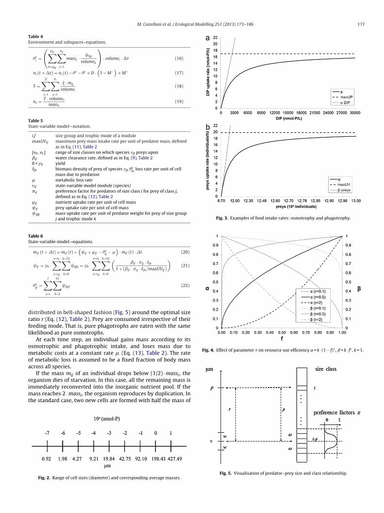
The nutrient affinity ˛ij and prey clearance rate ˇij (Eqs. (8) and(9), Table 2) define the slope of the functional response curves (Eqs.(5) and (6), Table 2) at low resource concentrations. Their decreasewith the square of the cell diameter implements the size penaltypostulated by Thingstad et al. (2010).

At high resource concentrations, the phosphorous and preyuptakes asymptotically approach the maximum rates maxUPij andmaxUVij. The maximum intake rates depend on the cell traits(standard mass and foraging mode), and on � (Eqs. (10) and (11),Table 2).

The third factors on the right hand sides of Eqs. (8)–(11) reflectthe decrease in resource uptake efficiency and maximum uptakerates of mixotrophs compared to osmotrophic and heterotrophicspecialists (Tittel et al., 2003). The magnitude of the efficiency lossis adjusted via the parameter �. Fig. 4 depicts the effect of � on ˛ijand ˇij.

Predators of a given size class i eat prey within a fixed range[v0i, vLi] of size classes (Eq. (6), Table 2). They have maximum pref-

erence for individuals smaller by a diameter ratio r (� size classes),where r is a fixed system parameter. The preference factors �ik ∈ [0,1] for predators of size class i for prey of size class k ∈ [v0, vL] are

(5)

(6)

(7)

(8)

(9)

(10)

(11)

(12)

(13)

(14)

(15)

M. Castellani et al. / Ecological Modelling 251 (2013) 173– 186 177

Table 4Environment and subspaces–equations.

vi

=

(pLi∑k=p0i

nk∑j=1

massj · kji

volumek

)· volumei · �t (16)

ni (t + �t) = ni (t) − v − s + D ·(

1 − M−)

+ M+ (17)

T =˙∑i=1

ni∑j=1

· mijvolumei

(18)

nz = T · volumezmassz

(19)

Table 5State-variable model—notation.

i,f size group and trophic mode of a modulemaxUVif maximum prey mass intake rate per unit of predator mass, defined

as in Eq. (11), Table 2[v0, vL] range of size classes on which species �if preys uponˇif water clearance rate, defined as in Eq. (9), Table 20 < �0 yieldıjk biomass density of prey of species �jk

vik

loss rate per unit of cellmass due to predation

� metabolic loss rate�if state-variable model module (species)�ij preference factor for predators of size class i for prey of class j,

defined as in Eq. (12), Table 2ϕif nutrient uptake rate per unit of cell mass if prey uptake rate per unit of cell mass ifjk mass uptake rate per unit of predator weight for prey of size group

j and trophic mode k

Table 6State-variable model—equations.

mif (t + t) = mif (t) +( if + ϕif − v

if− �)

· mif (t) · t (20)

if = �0 ·j=vL∑j=v0

k=32∑k=0

ifjk = �0 ·j=vL∑j=v0

k=32∑k=0

(ˇif · �ij · ıjk

1 + (ˇif · �ij · ıjk/maxUVif )

)(21)

l∑ 32∑

drfl

omoa

oimt

Fig. 3. Examples of food intake rates: osmotrophy and phagotrophy.

Fig. 4. Effect of parameter � on resource use efficiency ̨ = k · (1 − f)� , ̌ = k · f� , k = 1.

vif

=j=s k=2

jkif (22)

istributed in bell-shaped fashion (Fig. 5) around the optimal sizeatio r (Eq. (12), Table 2). Prey are consumed irrespective of theireeding mode. That is, pure phagotrophs are eaten with the sameikelihood as pure osmotrophs.

At each time step, an individual gains mass according to itssmotrophic and phagotrophic intake, and loses mass due toetabolic costs at a constant rate � (Eq. (13), Table 2). The rate

f metabolic loss is assumed to be a fixed fraction of body masscross all species.

If the mass mij of an individual drops below (1/2) · massi, therganism dies of starvation. In this case, all the remaining mass is

mmediately reconverted into the inorganic nutrient pool. If the

ass reaches 2 · massi, the organism reproduces by duplication. Inhe standard case, two new cells are formed with half the mass of

Fig. 2. Range of cell sizes (diameter) and corresponding average masses.Fig. 5. Visualisation of predator–prey size and class relationship.

178 M. Castellani et al. / Ecological Modelling 251 (2013) 173– 186

Fd

teimc

eie

e(ttp

c�p

3

eamd

tpSdb

ibioc(

3

dfdc

aai

Fig. 7. Flow of biomass between two sample classes and the DIP pool. Thephagotrophs and mixotrophs of size class i prey upon the individuals of class j(predator–prey ratio is �). The total biomass intake of the predators of class i is

needs.

ig. 6. Iterative procedure to calculate the number of individuals killed due to pre-ation.

he parent cell. Namely, the new cells are initialised with a weightqual to the standard mass massi of its size class. The new cellsnherit the trophic mode of the parent. However, occasional genetic

utations may alter the traits (size and foraging mode) of the dupli-ated individuals.

The probability of mutation mutRate ≤ 1 is a fixed system param-ter. At every duplication event, a random number rand ∈ [0, 1]s sampled. If rand < mutRate, the new individual undergoes withqual probability mutation of either the size or the feeding mode.

If a new individual undergoes a mutation in size, it will join withqual probability either the next smaller or the next larger size classEq. (14), Table 2). Eq. (14) accounts for the different volumes ofhe subspaces of origin and destination of the mutant, and scaleshe mass of the mutated individual up or down to keep the totalhosphorous density ıP constant.

If a new individual undergoes a mutation in trophic mode, thehange ı in the parameter fij occurs within a limited range [−�,] from the mother trait (Eq. (15), Table 2), where � is a systemarameter (Table 7).

.2. Subspaces

Each size group i is modelled within a sub-space of the overallnvironment. The volume (volumei) of this sub-space is calculateds in Eq. (1), and kept constant throughout the simulation. The twoain features of a subspace are its volume and the total biomass

ensity of the hosted population.In each time step, predation from other size classes may lead

o mortality. The biomass vi

of size class i eaten by predators of aarticular size class follows Holling Type 2 curves (Eq. (6), Table 2).ummation over all predator classes gives the total amount eaten,vi

(Eq. (16), Table 4). Individuals of a prey class are killed ran-omly until the number of individuals (v) corresponds to the killediomass (v

i) (Fig. 6).

At the end of every time step �t, the population size ni of class is updated (Eq. (17), Table 4). Eq. (17) takes into account the num-er of individuals dead due to starvation (s) the number of new

ndividuals created by cell duplication events (D), and the numberf mutants lost to (D · M−) and acquired from (M+) neighbouringlasses. The size class biomass density is then recalculated as in Eq.2).

.3. Environment

The environment is composed of the ̇ subspaces, where theifferent size groups and the DIP pool are modelled (one subspaceor each size group). The environment is assumed to have uniformensity in terms of spatial distribution of the populations and DIPontent.

The DIP pool is depleted by the activity of the mixotrophs

nd osmotrophs, and is replenished by the excretions, detritus,nd dead bodies produced by the ̇ populations. The only directnteraction between populations is given by the predation of large

ij , corresponding to v class j individual killed. Osmotrophs and phagotrophs ofthe two classes consume DIP. The DIP pool is refilled by the detritus, excretions, anddead bodies produced by the two classes.

individuals on smaller organisms. Fig. 7 visualises the biomass flowwithin the system for two sample species.

In biological systems, spatial heterogeneity allows species tosurvive in some areas when unfavourable conditions may lead totheir extinction elsewhere. The surviving populations may then re-colonise the empty niches and thrive when conditions change. Anextra procedure was designed to simulate the possible reintroduc-tion of locally extinct species.

The additional procedure introduces individuals of a randomlypicked size class at fixed time steps. If conditions are favourable, thenew individuals form a stable population. This process simulatesoccasional invasions of alien species in ecological subsystems. Itworks as follows: each living individual is “taxed” of a small fraction of its body mass (Eq. (18), Table 4). This tax simulates the loss ofindividuals that moved to neighbouring regions outside of the mod-elled area. It is then used to create nz new members of a randomlyselected size class z (Eq. (19), Table 4), simulating the immigrationof individuals from contiguous areas. The foraging mode of thesenew agents is randomly initialised.

4. State-variable model

To evaluate the reliability of the proposed modelling approach,two conditions need to be checked: that the predictions on theemerging food web structure are biologically realistic, and that theyare not affected by computational artefacts.

Unfortunately, accurate quantitative descriptions of pelagicmicrobial communities are still lacking. Yet, qualitative evaluationson the plausibility of the model predictions are possible.

To ascertain the presence and extent of computational artefacts,the results of the individual-based model are compared with thoseof an equivalent state-variable model. If the differences are large,the results of the two models will have to be treated with cautionuntil the issue is further resolved. If the two models yield similarpredictions, the results can be assumed to be independent of imple-mentation issues. In case the two models perform comparably, itwill also be possible to use them interchangeably according to the

The state-variable model is composed of a matrix of ̇ × 32modules, dividing the food web into ̇ size classes and 32 classesof feeding modes. The ̇ size classes correspond one-by-one to

M. Castellani et al. / Ecological Modelling 251 (2013) 173– 186 179

Table 7Standard settings for the system parameters of the individual-based (IBM) and state-variable (SV) models.

Parameter Symbol Value Model

Main looptotal phosphorous concentration ıP 500 (nmol-P/L) IBM/SVnumber of size groups Ns 32 IBM/SVmax number of individuals per group N 10000 IBMmass smallest individual mass1 1.6·10−8 (nmol-P) IBM/SVdiameter smallest individual diam1 0.5 (�m) IBM/SVmass increment factor between successive size groups 2 IBM/SV

nutrient affinity smallest osmotroph (per unit of biomass) ˛0 0.7(Lh

· 1nmol−P

)IBM/SV

max uptake rate smallest osmotroph (per unit of biomass) maxUP0 0.16(nmol−Ph

· 1nmol−P

)IBM/SV

water clearance rate smallest phagotroph (per unit of biomass) ˇ0 0.0008(Lh

· 1nmol−P

)IBM/SV

max prey biomass intake rate smallest phagotroph (per unit of biomass) maxUV0 3.125(nmol−Ph

· 1nmol−P

)IBM/SV

yield �0 0.3 IBM/SVmixotrophy trade-off � 0.3 IBM/SVoptimal predator–prey ratio � 4 (6 size classes) IBM/SVwidth predator–prey size window ω 1.26 (1 size class) IBM/SVmutation rate mutRate 0.02 IBMwidth of feeding mode mutation � 0.1 IBMgeneral loss rate � 0.001 (1/h) SVmetabolic loss rate � 0.001 (1/h) IBM

tfo

(tid(

Tom

5m

sttff

icgic

usIr

fhtstb

Initialisation procedurefraction of total P into DIP

“noise” in mass distribution amongst classes

he size classes used in the individual-based model, whilst the 32eeding modes cover at fixed steps of 0.03125 the range from puresmotrophy (0) to pure phagotrophy (1).

The increment of biomass is determined for each modulespecies) �if by the nutrient and prey uptake, loss due to preda-ion, and metabolic losses (Eq. (20), Table 6). Analogously to thendividual-based model, nutrient and prey uptake as well as lossue to predation follow Holling Type 2 functional responses (Eq.5), Table 2, and Eqs. (22) and (23), Table 6, respectively).

The differential equation of the state-variable model (Eq. (21),able 6) is integrated using the MATLAB ODE23 implementationf the explicit Bogacki and Shampine third-order Runge-Kuttaethod (Shampine and Reichelt, 1997).

. Differences between individual-based and state-variableodel

The equations defining the dynamics of the two models are theame. They differ only in the fact that in the individual-based model,hey apply to one individual, whilst in the state-variable model,hey apply to the whole biomass of the functional group. This dif-erence accounts for the fact that the agents are individuals in theormer and whole species (modules) in the latter.

The trait-based model discretises the biomass of one size classnto several units (the agents), whilst the state-variable model dis-retises the trophic structure of the size classes into 32 functionalroups. That is, in the state variable model, the ‘feeding mode’s discretised into regularly spaced steps within each of the sizelasses.

The above differences can be minimised choosing large pop-lation sizes, and partitioning the functional groups of thetate-variable model into finely divided classes of feeding modes.n both cases, the correct parameterization needs to trade-off rep-esentation power for efficiency.

In the state-variable model, biomass is a continuous variableor each size group. As a result, the mass content of a group mayappen to drop below the mass equivalent of one organism. In

his case, unless explicitly stated in the model implementation, thepecies does not become extinct. In the individual-based model,he biomass is discretised in individual units. Once its biomass iselow (1/2) · massi it dies, and once the last individual has died,

0.001 IBM/SV0.1 IBM/SV

the species is lost. This dissimilarity makes the populations of thestate-variable model more robust to environmental fluctuations.This is one of the fundamental differences between individual-based and state-variable representations, and is independent of theimplementations chosen in this study.

The discretisation of the biomass in individual units in theindividual-based model has also consequences on the effects ofpredator–prey interactions. That is, in a state-variable model apredator may consume an amount of mass equivalent to a fractionof a prey (e.g. a lion eats half a gazelle); the remaining fraction ofprey still survives and contributes to the total biomass of its species.In an individual-based model, the partly eaten prey cannot survive,and the remains are usually discarded as detritus. As a consequence,the activity of predators has a greater impact on the prey popula-tion in individual-based models. In the proposed individual-basedmodel, the discarded remains correspond to at most a fraction ofone individual (see Eq. (16), Table 4). Even though this amount maybe considered small in a large population, in a small population orover several time steps, it might lead to appreciable discrepanciesbetween the predictions obtained using the individual-based andthe state-variable model.

In the proposed study, genetic mutations are used only in theindividual-based model. This feature is expected to blur the shapeof the emergent population structure. It was created to promoteinnovation in species, and partly compensate for the likelihoodof extinction events in individual-based models. Mutations mayin fact reinstate extinct species, reducing the loss of populationdiversity in individual-based systems.

6. Experimental tests

This section describes the experimental settings and results.

6.1. Experimental settings

For the parameters of the two models, the standard setting andthe dimensions are given in Table 7.

Initially, 0.1% of the total phosphorous concentration consti-tutes the DIP pool, and the rest is shared amongst the size groups.This scenario simulates an oligotrophic environment, which is thetypical state of pelagic ecosystems.

1 al Modelling 251 (2013) 173– 186

oyt(qm

m

wt(

oai(tksi

iIutibtmm

a7w

6

ic

dsspdge

rct

tawro

1mbea

80 M. Castellani et al. / Ecologic

The maximum hourly phosphorous uptake rate for the smallestsmotroph (maxUP0) is set equal to one sixth of the cell’s weight,ielding a duplication time of six hours in absence of food limita-ion. The maximum prey uptake rate for the smallest phagotrophmaxUV0) is set equal to 200 individuals per cell per hour. Thisuantity is converted into units of prey mass per unit of predatorass as follows:

ax UV0 = mv

mp· 200 = mv

mv · 2�· 200 = 1

2�· 200 (23)

here mp and mv are the weights in phosphorous of respectivelyhe predator and the prey, and � is the size ratio of predator to preyhenceforth called predator–prey ratio).

The above values were set in accordance with experimentalbservations on the maximum nutrient affinity (Lignell et al., 2013)nd uptake rate (Kemp et al., 1993) for pure osmotrophs, and max-mum clearance rate (Lignell et al., 2013) and prey uptake rateVaquè et al., 1994) for pure phagotrophs. Other parameters likehe mixotrophy trade-off and predator–prey ratio are at present notnown precisely (Stoecker, 1998), and were set heuristically. Theensitivity of the predictions to these less understood parameterss the object of a separate study.

Four groups of experiments were run to investigate the sensitiv-ty of the predictions to the choice of the main model parameters.n all cases, 10 independent runs were executed per model config-ration. For each run, the system was let to evolve for 10 years withime steps of 5 min. At the end of the evolution period the emerg-ng populations were monitored for one additional year, where theiomass distribution was sampled every five days. A final map ofhe average biomass distribution amongst size classes and feeding

odes was generated for the last year. This map represents theodel prediction.The code was implemented in C++, and the tests were run on

n Intel Core2 Duo CPU, 2.54 GHz speed, 4GB Ram, and Windows 32-bit OS. In all cases unless explicitly stated, the execution timeas less than 20 min per run.

.2. Sensitivity to initialisation procedure

The first set of experiments was designed to test the sensitiv-ty of the model predictions to the initialisation of the microbialommunity. Three initialisation procedures were tested.

The first procedure (henceforth named ‘deterministic–eterministic’) distributes the biomass uniformly amongst theize classes, and uniformly amongst the individuals within theize classes. That is, each agent is initialised with a weight in phos-horous equal to the class standard massi (Eq. (3)). This uniformistribution of biomass amongst the logarithmically spaced sizeroups simulates the natural state of planktonic systems (Sheldont al., 1972).

The second procedure (henceforth named ‘deterministic–andom’) distributes the biomass uniformly amongst the sizelasses, and initialises the mass of each individual randomly withinhe interval [minmassi, maxmassi] Section 3.2).

The third procedure (henceforth named ‘random–random’) dis-ributes the biomass randomly amongst classes, and randomlymongst the individuals. For each class, the initial biomass is drawnith uniform probability within ±10% of ıP/˙.,here ıP and ̇ are

espectively the total phosphorous in the system, and the numberf size classes (Section 2.2).

Fig. 8 shows the statistical mean of the predictions obtained in0 independent runs for each of the three cases. The microbial com-

unity is divided into 32 size classes (Table 1), each characterised

y a specific diameter and mass (see Section 3.2 and Fig. 2). Forach size class, the emergent population is grouped into 32 classesccording to the feeding mode. The map represents thus a 32 × 32

Fig. 8. Comparison of initialisation procedures. Model parameters as in Table 7.

matrix of size and foraging mode classes. The mass distributionis plotted versus the average cell mass of the size classes and thefeeding mode.

The plots show very similar results, with stable populations ofmixotrophs emerging roughly within the 2–4 �m diameter range.The evolved mixotrophic populations are in the size range of bacte-ria (0.2–2 �m) and nanoflagellates (2–20 �m).

Populations of pure osmotrophs emerge in a size range withinthe smallest allowed diameter (0.5 �m) and 3 �m circa.

Two populations of pure phagotrophs appear: one of ca. 2–3 �mdiameters, and the other of ca. 4–13 �m diameters. The latter pop-

ulation is within the size range of dinoflagellates (5–2000 �m). Thegroup of largest phagotrophs preys on the microbial communitiesin the 2–4 �m range (the predator–prey ratio was set to 4), whilst

M. Castellani et al. / Ecological Modelling 251 (2013) 173– 186 181

F tion sii

to

bcUTtwo

ig. 9. Sensitivity of the results to the variation of the number and maximum populanitialisation procedure is used.

he population of smaller phagotrophs preys on the smallest classesf osmotrophs.

The significance of the differences between the maps ofiomass distribution obtained using the three initialisation pro-edures was analysed pixel-by-pixel using the Mann–Whitney-test. The analysis confirmed the high similarity of the results.

he two most dissimilar maps were those obtained usinghe deterministic–deterministic and deterministic–random methods,here the biomass values differed significantly in 13 pixels (1.27%

f total map).

ze of the size classes. Model parameters as in Table 7, the deterministic–deterministic

Given the substantial equivalence of the different initialisationroutines, the deterministic–deterministic method will be used as thestandard procedure henceforth.

6.3. Sensitivity to model configuration

The second set of experiments (Fig. 9) was devised to investigatethe robustness of the predictions to variations of model parameterssuch as the number of size classes (˙), and the maximum class size(N).

182 M. Castellani et al. / Ecological Modelling 251 (2013) 173– 186

Fig. 10. Sensitivity of the results to variations of the mutation rate. Model parameters as in Table 7, the deterministic–deterministic initialisation procedure is used.

orin

tei

tvpdmdNmwbap

The emergent populations are substantially similar regardlessf the number of size classes. Due to the lower resolution, the mapelative to the case ̇ = 16 has a better delineated shape. As ˙ncreases, the microbial community breaks down in an increasingumber of smaller populations.

The relationship between the maximum population size N andhe algorithm running time appears to be roughly linear. Forxample, enlarging N from 10000 to 40000 agents per size groupncreased the execution time from 20 min to over 90 min.

The use of larger populations reduced the risk of extinction forhe individual species. This favoured the establishment of moreariegate microbial communities in the tests involving the largestopulation sizes. A pixel-by-pixel comparison between the pre-ictions found 43 (4.2%) significantly different pixels between theaps obtained using N = 5000 and N = 10000, 41 (4%) significantly

ifferent pixels between the maps obtained using N = 10000 and = 20000, and 93 (9.1%) significantly different pixels between theaps obtained using N = 5000 and N = 20000. The significance tests

ere carried out using the Mann–Whitney U-test. The overall

iomass distribution is, however, similar in all the cases, indicatinglso in this case robustness of the model to variations of the systemarameters.

6.4. Effects of mutation and reintroduction of species

The third set of experiments was designed to assess the effectsof the mutation (Section 3.2) and reintroduction (Section 3.4) pro-cedures on the model predictions.

Mutation played a decisive role for the maintenance ofpopulation diversity (Fig. 10). Without mutation, mixotrophs dis-appear and the population clusters into three groups of pureosmotrophs and three corresponding groups of predators. Asthe mutation rate is increased, the plots show a progressivelythicker band of mixotrophs establishing. The populations ofpure osmotrophs and phagotrophs become also more broadlydistributed.

The map obtained using the standard mutation rate (0.02)and those obtained using higher rates (0.05 and 0.1) differ sig-nificantly by 52 (5.07%) and 89 (8.7%) pixels respectively. In allthe three cases, the distribution of the emergent population issimilar.

If performed with sufficient frequency, the reintroduction pro-cedure (Fig. 11) can compensate for the loss of species. However,it introduces a certain degree of ‘noise’ in the individual runs. Theemergent biomass distribution is similar to the standard case.

M. Castellani et al. / Ecological Modelling 251 (2013) 173– 186 183

F el para

6

potorf(p

7

tdnsinoe

ig. 11. Sensitivity of the results to variation of the reintroduction procedure. Mod

.5. Comparison with state-variable model

The fourth set of experiments concerns the comparison of theredictions obtained using the individual-based model with thosebtained using the state-variable model. Following the results ofhe theoretical study presented in Section 6, the metabolic loss ratef the individual-based model was set equal to the general lossate of the state-variable model (see Table 7). Good agreement wasound between the predictions obtained using the two approachesFig. 12), with populations of mixotrophs, pure osmotrophs andhagotrophs emerging at the same size ranges.

. Discussion

The Scaled Subspaces Method models the evolution of popula-ions of largely diverse traits and density with the same degree ofetail, eliminating the risk of demographic explosion of the mostumerous species. In order to limit the population size, increasinglymaller-sized species are modelled in increasingly smaller spaces,

n the same way microbiologists choose objectives of increasinglyarrower field to observe increasingly smaller organisms on anptical microscope. This makes the proposed method intuitivelyasy to understand and visualise. Also, when we are interested in

meters as in Table 7, deterministic–deterministic initialisation procedure is used.

how organism strategies lead to emergent patterns in the topologyof the population within the strategy plane (i.e. the cell size andtrophic mode trait-space), it is important that biological represen-tations are continuous and equally diverse over all size classes. Asopposed to approaches that combine state variables and individual-based descriptions (Megrey et al., 2007), our Scaled SubspaceMethod allows this.

The Scaled Subspaces Method can be implemented in fast andcompact software code. The effectiveness of the proposed methodwas demonstrated in an application of modelling a microbial foodweb.

Experimental evidence proved that the Scaled SubspacesMethod generates consistent and realistic population distribu-tions. It is thus a viable alternative to trait-based approaches usingsuper-individuals (Scheffer et al., 1995; Woods and Onken, 1982;DeAngelis et al., 1993) to deal with the problem of unmanage-ably large populations. With respect to the latter approaches, theproposed method may be conceptually and computationally moresimple, as it does not involve bookkeeping efforts (e.g. splitting and

merging of super-individuals) to maintain the population withingiven boundaries. This also minimises the possibility of introducingcomputational artefacts with respect to biodiversity in the mod-elling results.

184 M. Castellani et al. / Ecological Mod

Fig. 12. Comparison between the predictions obtained using the individual-bd

SitsoaSatoranaTstr

M

distribution of species, since some of the offspring of the most abun-

ased and state-variable models. Model parameters as in Table 7, theeterministic–deterministic initialisation procedure is used for both models.

There are similarities between the single individuals used in thecaled Subspaces Method and super-individuals. Agents modelledn small subspaces implicitly represent several individuals overhe whole system. In this sense, every individual in the scaledubspaces can be seen effectively as a representative of manythers. However, the representativeness (i.e. how many organismsn agent represents) of each individual is constant in the Scaledubspaces Method, whilst it varies with the stochastic events inpproaches using super-individuals. In the latter, it is often the casehat several similar super-individuals of highly different size (e.g.ne large and several small) coexist. Without the need of constantearranging of super-individuals, the Scaled Subspaces Methodllows one to model with uniform representativeness a largeumber of individual types. This makes the proposed approach

good candidate for modelling biodiversity at all trophic levels.he uniform detail in the representation of the species at diverseize scales makes the Scaled Subspaces Method particularly usefulo model fractal-like biological systems, where self-similarity is

epeated at largely different scales (Thingstad et al., 2010).

The comparison of the predictions given by Scaled Subspacesethod with those given by an equivalent state-variable model

elling 251 (2013) 173– 186

with high resolution in organism size and foraging mode ensuredthe independence of the results from implementation issues. Thetest also gave the occasion to analyse the expected differencesbetween trait-based and state-variable models.

The Scaled Subspaces Method implicitly assumes the environ-mental conditions to be spatially uniform, meaning that the focusof the model can be narrowed down to a small area without lossof generality. This was assumed for the simplified representationof the marine microbial food web used in this study. In other casesthis assumption may not be true. A possible way to circumventthis problem would be to simulate the evolution of communities ofspecies in different environments in parallel. Each species would bedefined in a subspace where the environmental conditions mightbe considered uniform, and plausible rules of interaction should bedevised for those species that are capable of migrating and operat-ing across different subspaces. The feasibility of this solution shouldbe weighed against the computational overheads that it wouldimply.

The scaling of the subspaces was here based on the total biomassin the closed system. In cases where the overall biomass varieswith time, the approach is still applicable as long as the changeis within reasonable bounds. In extreme cases, where the totalbiomass changes of several orders of magnitude, the size of thesubspaces could be adjusted at periodic intervals, or when oneor more populations reach a pre-set upper or lower size thresh-old. Such adjustments are possible as long as the fluctuations ofnutrients are not too frequent. In particularly variable ecosystems,where the total biomass changes rapidly of several orders of mag-nitude, other approaches such as the use of super-individuals arecomputationally more efficient.

In general, the scaling of the subspaces may take into accountother criteria than the potential for population abundance. Forexample, where some species have a greater potential for hetero-geneity (e.g. they have more traits), the scaling of the subspaces maytake into account additional or alternative considerations, such asthe possibility of population diversity.

Beyond the uniformity of the environmental conditions, the onlyother assumption made in the Scaled Subspaces Method is that theeffect of the interactions of each species with the other species andthe environment can be computed from the population (biomass)density. The details of the interactions may be expressed analyt-ically as in the proposed application, or probabilistically on anindividual-to-individual basis. The trait-based paradigm allows therepresentation of any level of high intra-class and inter-class diver-sity. As long as the impact of the populations on the ecosystem canbe expressed in terms of their population density, communities ofspecies as heterogeneous as ants and elephants can be simulated.

One of the main difficulties in modelling ecosystems is to sim-ulate a large and virtually unbound world in a limited and closedsystem. In this sense, closed ecosystem models are more similarto laboratory set ups than natural environments. In such kind ofscenarios, with relatively small population numbers and constantenvironmental conditions, the extinction of all but a few speciesis likely. In nature, the distribution of organisms is inhomoge-neous, and individuals migrate in and out of local environments.In the presented application of the Scaled Subspaces Method, wewanted to simulate mechanisms found in the open sea whereabundant species disperse to neighbouring areas, and where otherspecies enter and re-colonise local environments when conditionsare favourable. As an extension for the new method, the reintro-duction procedure was designed for this purpose. Mutation alsoplays a role in reinstating populations and balancing the overall

dant classes mutate into similar species that got extinct. Mutantsoccur naturally, and they may be able to colonise vacant niches.Genetic mutations, periodic reintroduction of species, and the use

l Mod

otawsab

posdaaesew

atadarae

aoMsar

8

tedbstieopooias

pbScattaipi

M. Castellani et al. / Ecologica

f large populations were shown to be effective policies againsthe extinction of species in our model. Nonetheless, state-variablepproaches might offer better protection from group extinctionshen the populations are known to undergo large oscillations in

ize. In general, the maintaining of population diversity in closednd bound environments is a common problem to all individual-ased discrete approaches.

Mixotrophs seem more at risk of extinction in our model thanure foraging specialists. However, this result was found to dependn the particular value chosen for the mixotrophy trade-off � (nothown). In general, the issue of the sensitivity of the model pre-ictions to variations of the biological parameters has not beenddressed in this study. Many of the parameters listed in Table 7 andllometric relationships defined in Tables 2, 4 and 6 are only beststimates. Sensitivity to biological parameters is subject to anothertudy, where the proposed model is used to help understand theffect of these variables on the structure of the emerging foodeb.

It can be argued against the biological realism of the mutationnd reintroduction procedures used in this study. We believe thathey are reasonably “natural” as long as open marine environmentsre to be modelled. The rate and extent of the mutation and reintro-uction events used in this study may possibly not be biologicallyccurate, and the model may conceivably be parameterized moreealistically. Indeed, more than suggesting a fixed set up, our testsimed to highlight the role of mutation and reintroduction on thevolution of the ecosystem modelled.

In general, this paper presented a first documentation of thepplicability and reliability of the Scaled Subspaces Method in casef microbial food webs, which are fundamental to all ecosystems.icrobial food webs are particularly well suited for the Scaled Sub-

pace Method due to their self-similarity and different densitiest many scales. The precise boundaries and details of the methodsange of application need to be thoroughly investigated.

. Conclusions and indications for further work

This paper presented the Scaled Subspaces Method, a newrait-based approach that addresses the problem of demographicxplosion in models composed of populations of inhomogeneousensity. The method was applied to a model of a pelagic micro-ial mixotrophic food web, where the population density of thepecies of smallest size is several orders of magnitude higherhan the density of the largest species. For each size group, thendividuals are monitored at different size scales. The small-st individuals are monitored at scales small enough to containnly a limited number of agents. With this we keep com-utational costs low, whilst still allowing equal diversificationf species at all levels. Also, computational artefacts that mayccur through bookkeeping and non-uniform representativenessn super-individuals, is avoided. It hence represents a beneficiallternative method to the super-individual approach for complexystems.

Experimental evidence shows that the proposed modelroduces biologically plausible and consistent predictions ofiomass distribution in the foraging mode and cell size trait-space.imilar results were found for other settings of the biologi-al parameters not documented in this paper. The predictionsttained using the proposed individual-based model matched wellhose obtained using a classical state-variable model. This showshat the results are independent from computational artefacts

nd implementation issues, and allows using the two modelsnterchangeably. The comparison of the two approaches was com-lemented by a thorough analysis of the differences between

ndividual-based and state-variable representations.

elling 251 (2013) 173– 186 185

The main issue concerns the possibility of extinction of speciesin the proposed method, which is inherent to all individual-basedmodels, and does not depend on the representation method used inthis study. The problem can be alleviated by simulating the creationof new individuals via genetic mutations, or by reintroduction oflost species. The frequency of the mutation or reintroduction eventsshould take into account the need to create and support biologi-cal diversity as well as biological plausibility. Future work shouldinvestigate the relationship between the mutation and reintroduc-tion rate and population diversity.

Using large populations helps to prevent group extinctions.However, the computational overheads of managing a large num-ber of agents need to be taken in account when setting the size ofpopulations. State-variable or individual-based approaches basedon super-individuals might be more robust to group extinctionsthan the proposed method. Further work should test this hypoth-esis and investigate the “breaking points” (i.e. extinction eventsof entire groups) of the population diversity for the differentapproaches.

We found that mixotrophs in our model could successfullycoexist with foraging specialists under a range of parameter sett-ings. This result agrees well with the reported high abundance ofmixotrophs in pelagic environments (Zubkov and Tarran, 2008;Hartmann et al., 2012). We hold that the Scaled Subspaces Methodrepresents a novel, realistic and useful tool to the field of ecologicalmodelling.

Acknowledgement

The study was done as part of the MINOS project financed byEU-ERC (proj.nr 250254) and with the support of the NorwegianResearch Council.

References

Adioui, M., Treuil, J.P., Arino, O., 2003. Alignment in a fish school: a mixedLagrangian–Eulerian approach. Ecological Modelling 167 (1–2), 19–32.

Bartsch, J., Coombs, S.H., 2004. An individual-based model of the early life history ofmackerel (Scomber scombrus) in the eastern North Atlantic, simulating transport,growth and mortality. Fisheries Oceanography 13 (6), 365–379.

Beyer, J.E., Laurence, G.C., 1980. A stochastic model of larval fish growth. EcologicalModelling 8, 109–132.

Carlotti, F., Wolf, K.U., 1998. A Lagrangian ensemble model of Calanus finmarchicuscoupled with a 1D ecosystem model. Fisheries Oceanography 7 (3–4), 191–204.

DeAngelis, D.L., Cox, D.C., Coutant, C.C., 1980. Cannibalism and size dispersal inyoung-of-the-year largemouth bass: experiments and model. Ecological Mod-elling 8, 133–148.

DeAngelis, D.L., Gross, L.J., 1992. Individual-Based Models and Approaches in Ecol-ogy, Populations, Communities and Ecosystems. Chapman and Hall, New York.

DeAngelis, D.L., Rose, K.A., Crowder, L.B., Marschall, E.A., Lika, D., 1993. Fish cohortdynamics: application of complementary modeling approaches. The AmericanNaturalist 142 (4), 604–622.

Donalson, D.D., Desharnais, R.A., Robles, C.D., Nisbet, R.M., 2004. Spatial dynamicsof a benthic community: applying multiple models to a single system. In: Seu-ront, L., Strutton, P.G. (Eds.), Handbook of Scaling Methods in Aquatic Ecology:Measurement, Analysis, Simulation. CRC Press, Boca Raton, FL, pp. 429–444.

Fath, B., Jørgensen, S.E., 2001. Fundamentals of Ecological Modelling, 3rd ed. Elsevier,544 pp.

Flynn, K.J., Mitra, A., 2009. Building the “perfect beast”: modelling mixotrophicplankton. Journal of Plankton Research 31 (9), 965–992.

Giske, J., Mangel, M., Jakobsen, P., Huse, G., Wilcox, C., Strand, E., 2003. Explicit trade-off rules in proximate adaptive agents. Evolutionary Ecology Research 5 (6),835–865.

Grimm, V., Railsback, S.F., 2005. Individual-Based Modeling and Ecology. PrincetonUniversity Press.

Grünbaum, D., 1994. Translating stochastic density-dependent individual behaviorwith sensory constraints to an Eulerian model of animal swarming. Journal ofMathematical Biology 33 (2), 139–161.

Harte, J., 1998. Consider a Spherical Cow. A Course in environmental Problem Solv-ing. University Science Books, Sausalito, CA.

Hartmann, M., Grob, C., Tarran, G.A., Martin, A.P., Burkill, P.H., Scanlan, D.J., Zubkov,M.V., 2012. Mixotrophic basis of Atlantic oligotrophic ecosystems. PNAS 109(15), 5756–5760.

1 al Mod

H

H

H

H

H

K

L

L

M

P

R

S

S

86 M. Castellani et al. / Ecologic

avskum, H., Riemann, B., 1996. Ecological importance of bacterivorous, pigmentedflagellates (mixotrophs) in the Bay of Aarhus, Denmark. Marine Ecology ProgressSeries 137, 251–263.

ellweger, F.L., Bucci, V., 2009. A bunch of tiny individuals—Individual-based mod-eling for microbes. Ecological Modelling 220 (1), 8–22.

ellweger, F.L., Bucci, V., Hinsley, W., Field, T., Woods, J., Shi, Y., van Albada,G., Dongarra, J., Sloot, P., 2007. Creating individual based models of theplankton ecosystem. Lecture Notes in Computer Science, vol. 4487. Springer,Berlin/Heidelberg, pp. 111–118.

olling, C.S., 1959. Some characteristics of simple types of predation and parasitism.The Canadian Entomologist 91 (7), 385–398.

use, G., Giske, J., 1998. Ecology in Mare Pentium: An individual-based spatio-temporal model for fish with adapted behaviour. Fisheries Research 37,163–178.

emp, P.F., Lee, S., LaRoche, J., 1993. Estimating the growth rate of slowly growingmarine bacteria from RNA content. Applied and Environmental Microbiology 59(8), 2594–2601.

ignell, R., Haario, H., Laine, M., Thingstad, T.F., 2013. Getting the “right” parametervalues for models of the pelagic microbial food web. Limnology and Oceanog-raphy 58 (1), 301–313.

oreau, M., Naeem, S., Inchausti, P., Bengtsson, J., Grime, J.P., Hector, A., Hooper,D.U., Huston, M.A., Raffaelli, D., Schmid, B., Tilman, D., Wardle, D.A., 2001.Ecology—Biodiversity and ecosystem functioning: Current knowledge andfuture challenges. Science 294 (5543), 804–808.

egrey, B.A., Rose, K.A., Klumb, R.A., Hay, D.E., Werner, F.E., Eslinger, D.L.,Lan Smith, S., 2007. A bioenergetics-based population dynamics model ofPacific herring (Clupea harengus pallasi) coupled to a lower trophic levelnutrient–phytoplankton–zooplankton model: Description, calibration, and sen-sitivity analysis. Ecological Modelling 202 (1–2), 144–164.

arry, H.R., Evans, A.J., 2008. A comparative analysis of parallel processingand super-individual methods for improving the computational perfor-mance of a large individual based model. Ecological Modelling 214 (2–4),141–152.

ose, K.A., Christensen, S.W., DeAngelis, D., 1993. Individual-based modelingof populations with high mortality: A new method based on follow-ing a fixed number of model individuals. Ecological Modelling 68 (3–4),273–292.

cheffer, M., Baveco, J.M., DeAngelis, D.L., Rose, K.A., van Nes, E.H., 1995. Super-individuals a simple solution for modelling large populations on an individualbasis. Ecological Modelling 80 (2–3), 161–170.

hampine, L.F., Reichelt, M.W., 1997. The MATLAB ODE Suite. SIAM Journal on Sci-entific Computing 18 (1), 1–22.

elling 251 (2013) 173– 186

Sheldon, R.W., Prakash, A., Sutcliffe, W.H., 1972. The size distribution of particles inthe ocean. Limnology and Oceanography 17 (3), 327–340.

Stoecker, D.K., 1998. Conceptual models of mixotrophy in planktonic protists andsome ecological and evolutionary implications. European Journal of Protistology34, 281–290.

Thingstad, T.F., 2000. Elements of a theory for the mechanisms controlling abun-dance, diversity, and biogeochemical role of lytic bacterial viruses in aquaticsystems. Limnology and Oceanography 45, 1320–1328.

Thingstad, T.F., Havskum, H., Garde, K., Riemann, B., 1996. On the strategy of “eatingyour competitor”. A mathematical analysis of algal mixotrophy. Ecology 77 (7),2108–2118.

Thingstad, T.F., Strand, E., Larsen, A., 2010. Stepwise building of plankton functionaltype (PFT) models: A feasible route to complex models? Progress in Oceanogra-phy 84 (1–2), 6–15.

Thorbek, P., Topping, C.J., 2005. The influence of landscape diversity and hetero-geneity on spatial dynamics of agrobiont linyphiid spiders: An individual-basedmodel. BioControl 50 (1), 1–33.

Thygesen, U.H., Nilsson, L.A.F., Andersen, K.H., 2007. Eulerian techniques forindividual-based models with additive components. Journal of Marine Systems67 (12), 179–188.

Tittel, J., Bissinger, V., Zippel, B., Gaedke, U., Bell, E., Lorke, A., Kamjunke, N., 2003.Mixotrophs combine resource use to outcompete specialists: implications foraquatic food F webs. Proceedings of National Academy of Sciences of UnitedStates of America 100 (22), 12776–12781.

Vaquè, D., Gasol, J.M., Marrasè, C., 1994. Grazing rates on bacteria: the significance ofmethodology and ecological factors. Marine Ecology—Progress Series 109 (2–3),263–274.

Waite, A.J., Shou, W., 2012. Adaptation to a new environment allows cooperators topurge cheaters stochastically. Proceedings of the National Academy of Sciencesof the United States of America 109, 19079–19086.

Woods, J.D., 2005. The Lagrangian Ensemble metamodel for simulating planktonecosystems. Progress in Oceanography 67 (1–2), 84–159.

Woods, J.D., Onken, R., 1982. Diurnal variation and primary production in the ocean- preliminary results of a Lagrangian ensemble model. Journal of PlanktonResearch 4 (3), 735–756.

Woods, J.D., Perilli, A., Barkmann, W., 2005. Stability and predictability of a vir-tual plankton ecosystem created with an individual-based model. Progress in

Oceanography 67 (1–2), 43–83.

Yoshida, T., Jones, L.E., Ellner, S.P., Fussmann, G.F., Hairston, N.G., 2003. Rapid evolu-tion drives ecological dynamics in a predator–prey system. Nature 424, 303–306.

Zubkov, M.V., Tarran, G.A., 2008. High bacterivory by the smallest phyto-planktonin the North Atlantic Ocean. Nature 455, 224–227.