The Role of Temporary Help Employment in Low-wage Worker Advancement

Carolyn J. Heinrich LaFollette School of Public Affairs University of Wisconsin-Madison

Peter R. Mueser

Department of Economics University of Missouri-Columbia

Kenneth R. Troske

Department of Economics University of Kentucky

October 2007

This work was supported by a grant from the Rockefeller/Russell Sage Foundation Future of Work Program. We wish to acknowledge helpful comments from David Autor, Bernhard Broockman, John Fitzgerald, Gerald Oettinger, Jeffrey Smith, Daniel Sullivan, and participants in the NBER Conference on Labor Market Intermediation, the Third Conference on Evaluation Research (Mannheim), annual conferences of the Midwest Economics Association and the Society of Labor Economists, and seminars at the Bowdoin College and the Institute for the Study of Labor (IZA). Excellent research assistance was provided by Kyung-Seong Jeon and Chao Gu.

Abstract We examine the effects of temporary help service employment on later earnings and employment for individuals participating in three federal programs providing supportive services to those facing employment difficulties. The programs include Temporary Assistance for Needy Families, whose participants are seriously disadvantaged; a job training program with a highly heterogeneous population of participants; and employment exchange services, whose participants consist of Unemployment Insurance claimants and individuals seeking assistant in obtaining employment. We undertake our analyses for two periods: the late 1990s, a time of very strong economic growth, and shortly after 2000, a time of relative stagnation. Our results suggest that temporary help service firms may facilitate quicker access to jobs for those seeking employment assistance and impart substantial benefits as transitional employment, especially for individuals whose alternatives are severely limited. Those who do not move out of temporary help jobs, however, face substantially poorer prospects, and we observe that nonwhites are more likely than whites to remain in THS positions in the two years following program participation. Our results are robust to program and time period. Keywords: temporary help, mediated employment, program evaluation JEL Codes: J48, J26, J68

1

I. Introduction

The large increase in temporary help service (THS) employment in recent years—from less than

0.5 percent in 1982 to approximately 2.5 percent by 2004 (U.S. Bureau of Labor Statistics,

2005)—has been particularly dramatic for low-skilled, less-educated and minority workers, who

are now greatly overrepresented in the temporary help workforce (Autor and Houseman, 2005;

Heinrich, Mueser and Troske, 2005; DiNatale, 2001). This disproportionate concentration of

disadvantaged workers in THS employment, combined with the growing use of temporary help

service firms as labor market intermediaries by both private firms and public social welfare

programs, has engendered an active policy and research debate about the consequences of such

mediated employment for workers’ wages, job stability, access to fringe benefits, and labor

market advancement. In addition, the literature on the effects of THS employment has more

recently begun to address some of the more complex questions about the implications of

temporary help employment for workers’ labor market outcomes, including these workers’

subsequent labor market transitions, occupational mobility, and longer-term earnings trajectories.

In general, two competing arguments have been advanced about temporary help

employment: (1) employment through THS firms may provide a path to permanent and stable

employment for workers who might otherwise be excluded from such labor market

opportunities, and (2) temporary help jobs supplant productive employment search and reduce

access to better employment opportunities, ultimately depressing workers’ wages and

opportunities for advancement. The former argument is consistent with the basic premise

underlying current U.S. public welfare and employment and training policies, which assumes

that helping individuals to get jobs (even low-wage jobs) will give them the opportunity to gain

2

on-the-job skills and experience and move up the career ladder to better positions (i.e., “a foot in

the door” or a “stepping stone”). With this greater policy emphasis on short-term, work-oriented

social services, the role of THS firms in facilitating job placements has naturally grown,

particularly for disadvantaged workers served by such programs.

In order to examine whether employment in the temporary help industry helps or hurts

workers relative to other employment in the long run, we explore the subsequent employment

dynamics of workers in this industry and compare their experiences with those of workers who

either do not have jobs or who take jobs in other industries (i.e., in end-user firms). We focus

our analysis on individuals in the state of Missouri who have sought employment assistance or

cash support through any of three federal programs, Temporary Assistance for Needy Families

(TANF), a job-training or intensive work search program (Job Training Partnership Act in 1997,

Workforce Investment Act in 2001), and employment exchange services (Wagner-Peyser

services). It is not a goal of this study to understand the impact of participation in these three

programs, but rather to understand the impact of employment in the temporary help industry.

We draw individuals from each of these programs in order to identify a diverse sample of

individuals who are facing employment difficulties.

For many participants in these programs, entry into the program identifies a point of

potential crisis in their work lives or careers. Participants in the job training program and the

labor exchange services are explicitly seeking services to support employment efforts. The

TANF program is designed to provide support for low income families with children, but it

emphasizes entry into employment, and recipients who do not have an exemption face

employment and job training requirements. Our analysis allows us to consider the role that

3

temporary employment and other industries play at such critical junctures in determining future

labor market outcomes. Given that each program attracts individuals with markedly differing

employment histories, work opportunities and other demographic characteristics, separate

analyses of participants in these programs allow us to examine the role of selection into THS.

We begin our analysis by examining whether there are other industries that serve a role

similar to that of the temporary help industry. We observe that individuals in our sample are

particularly likely to move into temporary help employment when they enter these programs, and

we consider whether this pattern can be observed for any other industries. Next we look at

employment during the quarter following program entry, examining how employment and wages

two years later are influenced by the sector of this initial employment, and, in particular,

temporary help services. We limit the sample to those 18-64 years of age and conduct analyses

separately for men and women. We report analyses initially for those who begin participation

during calendar year 1997 and then consider analyses for those entering these programs in 2001.

Our use of large and long panels of state-level administrative data on participants in three federal

programs allows us to extend previous research on the effect of employment in THS by

examining the impact of THS over an extended period and at different points in the business

cycle and by comparing individuals who obtain employment in various industries and who have

very different demographic characteristics.

Our main findings are as follows. First, we find that THS is unique in serving as a

general transitional industry. Second, we find that working in the THS sector has very little

long-term negative impact on either earnings or employment for workers in any of the three

programs. If we believe that for workers in THS the next best opportunity in not having a job in

4

a quarter, working in the THS sector imparts significant benefits. Third, we find that worker

success is contingent on transitioning out of the THS sector; workers who remain in the THS

sector have long-run earnings that are substantially below workers in other sectors. Finally, we

find that our results are strikingly consistent across the business cycle, and that the experience of

nonwhites in THS jobs is very similar to that of whites.

In the next section we review the literature on the temporary help service industry. In

section III we discuss our data and in section IV we consider the role of the temporary help

service industry in providing transitional employment. We also examine the factors determining

who takes a temporary help job. Section V presents estimates of the impact of temporary help

employment on later earnings and employment, and section VI considers the role that

movements between jobs has in helping individuals achieve higher earnings and stable

employment. In section VII, we consider the degree to which results are replicated for

individuals participating in these programs in 2001 (a time when economic growth had slowed).

Section VIII focuses on the experience of nonwhites in temporary help jobs. Section IX turns to

the issue of how robust our results are if the OLS assumption of an independent error is violated.

The final section concludes.

II. Literature

There is strong agreement among a large number of studies that temporary help services jobs pay

lower wages, offer fewer work hours, are shorter in tenure, and are significantly less likely to

provide health insurance coverage or other fringe benefits (Autor and Houseman, 2005;

Andersson, Holzer and Lane, 2002; Blank, 1998; Booth, Francesconi and Frank, 2002; Cohany,

1998; Heinrich et al., 2005; Houseman and Polivka, 1999; Houseman, Kalleberg and Erickcek,

5

2003; Lane et al., 2003; Nollen, 1996; Pavetti et al., 2000; Pawasarat, 1997; Segal and Sullivan,

1997). A smaller number of studies go beyond descriptive statistics to examine the employment

and earnings paths or trajectories of welfare recipients and other low-wage workers who enter

temporary help services employment.

Using matched samples of “at-risk disadvantaged workers”1 from the Survey of Income

and Program Participation (SIPP), Lane et al. (2003) find that individuals who take temporary

help services jobs have better employment and “job quality” outcomes than those who do not

enter employment. Temporary help workers fare slightly worse than those who enter other

employment sectors in terms of earnings and benefits, although differences are generally small

and not statistically significant. In addition, they conclude that the effects of temporary help

employment in reducing welfare receipt and poverty relative to no employment are substantial,

and that there is no difference in these outcomes between those in temporary and conventional

employment.

Despite different populations of study (welfare recipients in Missouri and North

Carolina), the findings of Heinrich et al. (2005) mirror those of Lane et al. (2003). After

following welfare recipients who go to work for temporary help services for two years, Heinrich

et al. find very small differences (1-7 percent) in earnings between those who initially took

temporary help jobs and those who entered jobs in other sectors, with measured characteristics

explaining most of the differentials. The earnings of welfare recipients initially entering THS

jobs increased faster over the two-year period, in part due to their movement from temporary

1 Lane et al. (2003) use propensity score matching to define comparison groups of “at-

risk” workers (with incomes less than 200 percent of the poverty level) for their THS worker sample.

6

help into higher-paying industries. In addition, temporary help workers were no more likely to

be out of a job two years later and only slightly more likely to return to welfare than workers in

end-user firms, and they were substantially more likely to be employed and off of welfare two

years later than recipients without a job.

Andersson, Holzer and Lane (2002) use data from five states (California, Florida, Illinois,

Maryland and North Carolina) in the Longitudinal Employer Household Dynamics (LEHD)

program at the U.S. Census Bureau to analyze a sample of workers with persistently low labor

market earnings. Like Heinrich et al. (2005) they find that low-wage workers starting in THS

employment earn lower pay while employed by the temporary agency but that subsequent job

changes lead to higher wages and better job characteristics for these workers. Both Heinrich et

al. and Anderson et al. observe that low-wage workers who begin work with THS firms are more

likely to move to higher-paying industries, such as manufacturing, than those working in other

sectors (or not working). Such mobility provides the primary path through which temporary help

employment boosts later earnings; workers who do not leave the temporary help industry suffer

an earnings shortfall. Andersson, Holzer and Lane (2008) also use this five-state LEHD sample,

but consider a longer follow-up period and more sophisticated methods. Their results are

substantively similar.

Autor and Houseman (2005) take advantage of random assignment of welfare recipients

to welfare-to-work contractors, where contractors vary in their referrals to THS firms. Under the

assumption that such referrals are not correlated with other contractor practices that influence

client success, they estimate the effects of holding a THS job on low-skilled workers’ labor

market outcomes. Initial earnings increments among their THS workers do not persist, in part

7

due to declines in rates of employment, and THS workers fare more poorly over the subsequent

two years in terms of their earnings than “direct-hire” placements. Point estimates imply that

THS workers also earn less than welfare recipients with no job placements, although these

differences are not statistically significant. When they examine the impact of temporary help

employment using OLS, they obtain results consistent with others, that is, implying a substantial

benefit of temporary help employment, so their results differ from others because of their

identification methods, not because of their sample.

There is also a growing literature examining temporary help firms in Europe.2 Booth et

al. (2002) study temporary help employment in Britain using data from the British Household

Panel Survey and methods similar to Heinrich et al. and find temporary employment to be an

effective “stepping stone” to permanent employment. Kvasnikca’s (2005) study of temporary

help workers in Germany does not produce evidence that these workers are more likely to move

into permanent employment than unemployed workers, but neither does the analysis suggest that

they suffer any adverse effects from temporary work. In their study of temporary help workers

in Spain, Garcia-Perez and Munoz-Bullon (2005) find that temporary help workers in low

occupational groups had much lower probabilities of securing a permanent job than more skilled

workers. They concluded that these workers would have fared better had they not worked

through these intermediaries.

The findings of these and related studies speak to important, cross-national public policy

2 In the European literature, many studies examine jobs classified as “temporary” based

on the contract under which an individual is hired. Such jobs account for over 10 percent of employment in France and Germany, and over 30 percent of employment in Spain (Gagliarducci, 2005). We limit our review to European studies that consider mediated employment corresponding to the temporary help service sector in the U.S.

8

questions about the role of labor market intermediaries as a solution to the problem of low-wage

worker advancement (Poppe et al., 2003). A recent study by Even and Macpherson (2003) found

that “switching jobs is vital to significant wage growth among minimum wage workers,

particularly for young workers who find themselves in ‘low-training’ occupations” (p. 677).

And Andersson, Holzer and Lane (2005: 143) similarly concluded that “job changes account for

the vast majority of ‘complete’ transitions out of low earnings and even for most partial

changes.” We expect the results of our study to contribute to these policy debates about the role

of public and private intermediaries in helping workers connect with and advance in jobs.

The use of state-level administrative data allows us to expand the scope of our analyses

beyond these existing studies in several ways. First, the long panel allows us to follow workers

for an extended period after we first observe them in the temporary help industry. Our

replication of the analysis over two time periods enables us to examine whether the effect of

working in the temporary help industry varies across the business cycle. Second, because we

have large sample sizes, we are able to compare the effect of working in a variety of industries.

For example, we can compare the long-run impact of working in the temporary help industry

with the impact of working in another service industry or in the retail trade industry, which may

be the most relevant comparison for these workers. Finally, the fact that we have data from three

federal assistance programs, containing workers with very different characteristics and coping

with different types of employment shocks, allows us to examine the role that nonrandom

selection has on our results.

It is important to emphasize that the only “treatment” we are considering in this analysis

is the industry or employment sector of the firm into which individuals in our sample select after

9

entering one of these three public programs. We have no information in our data about whether

individuals who take temporary help services jobs are directed to these jobs by counselors in the

program. A 2001 survey of TANF recipients who had engaged in temporary help services

employment in North Carolina found that most (77 percent) did not learn about these jobs

through TANF counselors, but rather through other channels, including word-of-mouth,

newspaper ads, or by contacting the firm directly (Heinrich, 2005).

III. Data

Our basic sample consists of individuals who entered one of the three public programs described

above during 1997 or 2001. In each case, entry is defined as participation in a given quarter for

an individual who was not a participant in the prior quarter. An individual who entered one of

these programs during the year, exited and remained off for at least one quarter, and then

reentered, will be included twice in the file for a given year. The number of such cases is very

small. Information on program participation, as well as demographic information on individuals,

comes from data maintained by the state of Missouri to administer these programs.

TANF data are from Missouri’s Department of Social Services Income Maintenance file,

which includes information on services received for all program recipients. The data are

extracted on a monthly basis, and individuals are identified as new payees in a quarter if they are

receiving cash payments under this program in a given quarter and were not recipients in the

prior quarter. We omit a small number of payees who are males, in the two-parent program,

and/or receiving payments on behalf of “child only” cases.3

3 We omit payees in child only cases because these individuals are exempt from

employment and training requirements of the program.

10

Job training in 1997 was provided under the Job Training Partnership Act (JTPA),

identified on administrative files of Missouri’s Division of Job Development and Training

(administered within the Department of Economic Development). Job training in 2001 was

provided under the Workforce Investment Act (WIA), which replaced JTPA in July 2000 and

was administered within the same department in the new Division of Workforce Development.

All individuals enrolling in the “adult” or “dislocated worker” programs are included. 4 Under

JTPA, the adult program was means-tested, limited to individuals whose income in the prior six

months is below specified levels. Although WIA allows universal access, participants generally

have low earnings. Dislocated workers are typically individuals who have lost their jobs in firm-

wide layoffs. WIA regulations place less emphasis on job training than did JTPA, although, in

practice, participants for both programs are a select group of individuals who receive a level of

attention far beyond those who obtain employment exchange services, and we refer to

participants in both programs as undertaking “job training.”

Employment exchange files identify individuals who register for services provided under

federal Wagner-Peyser legislation.5 Most individuals who receive Unemployment Insurance

(UI) payments are required to register for these services and a substantial portion of job

exchange registrants are UI recipients. However, anyone in the state is eligible to use job

4 Since individuals in the adult program are younger, less well educated and have

dramatically lower prior earnings than those in the dislocated worker program, we undertook our basic analysis separately for these two groups. As differences in results were usually not statistically significant, we combined the adult and dislocated worker programs.

5 In 1997, the state’s job exchange service was administered by Missouri’s Division of Employment Security in the Department of Labor and Industrial Relations. In 1999, the program was transferred to the Division of Workforce Development in the Department of Economic Development.

11

exchange services, so registrants include employed individuals seeking better employment

prospects as well as other job seekers who are not receiving unemployment compensation.

Our data on earnings, employment history and the industrial classification of the job

come from the UI programs in the states of Missouri and Kansas. Earnings for individuals in a

quarter are reported by employers, and we are able to match these to program participants using

Social Security numbers. Although these data exclude the self-employed, those in informal or

illegal employment, and a small number of jobs exempt from Unemployment Insurance

reporting requirements, they include the overwhelming majority of employment in these states.

These data allow us to identify all employers for an individual during a quarter, but we cannot

determine whether jobs were held simultaneously or sequentially. A very small proportion of

Missouri residents hold jobs in states other than Kansas.6 All earnings in the analyses have been

adjusted for inflation based on the consumer price index using quarter 2 of 1997 as the base.

The industrial classification is taken from information about the employer on these files,

and our identification of temporary help workers is based on the convention that individuals

working on a temporary assignment from a THS firm are listed as employees of that firm.

Although the THS firm’s own direct employees (e.g., office staff) will also be included, the

proportion of such cases is expected to be small, especially among participants in the three

programs we are considering.7

6 Approximately one in six TANF residents in Jackson County, Missouri, the central

county for Kansas City, holds a job in Kansas. The proportion of St. Louis residents with jobs in Illinois is much smaller due to the depressed economy of East St. Louis, Illinois. No other significant concentrations of population are close to Missouri’s borders.

7 Antoni and Jahn (2007) report that 7 percent of the employees in temporary help firms in Germany are permanent administrative staff.

12

We have described these programs and their selection criteria, as we expect them to have

implications for the level of disadvantage and other characteristics of our sample members.

Tables A-1 and A-2 provide means and standard deviations for each of our samples in 1997 and

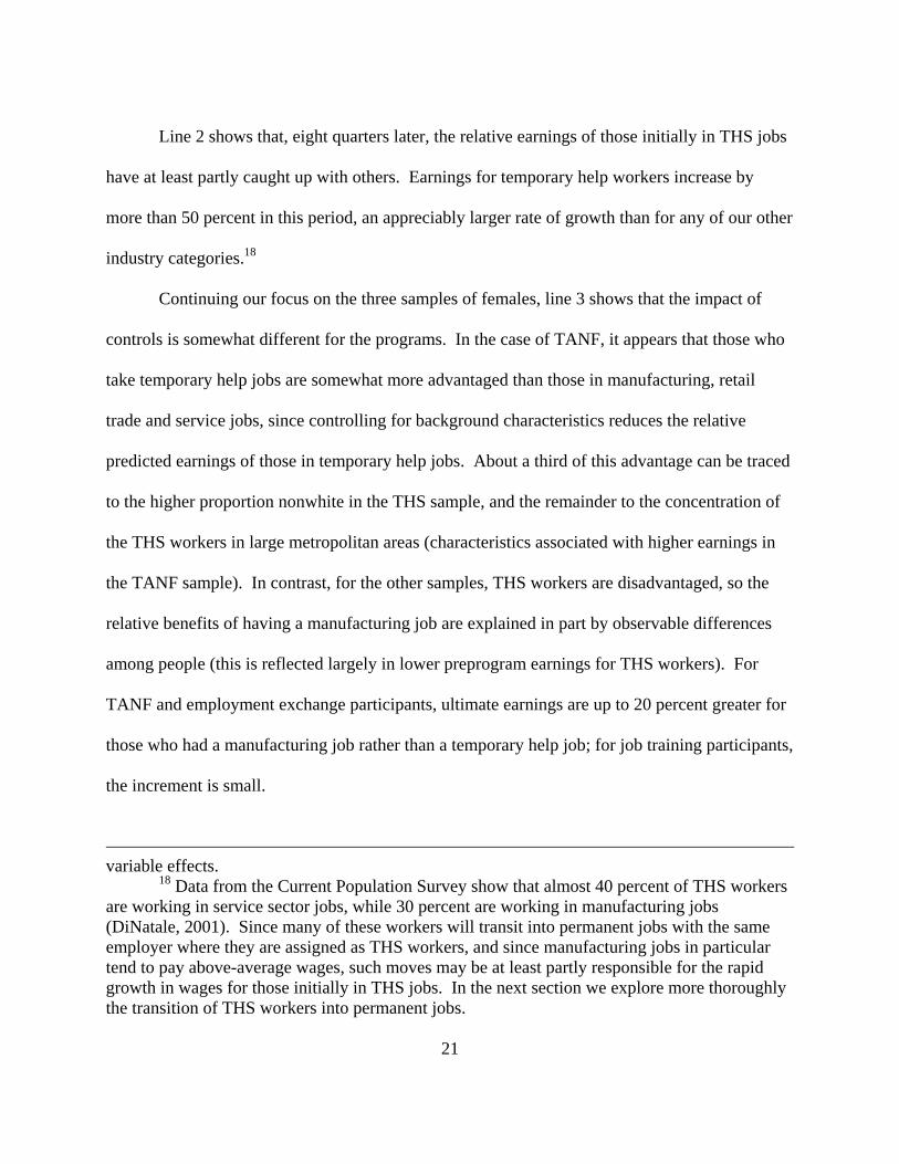
2001, respectively.8 Looking at the panels for females, the statistics confirm that TANF entrants

are substantially disadvantaged relative to the two other groups. For example, the mean number

of years of completed schooling for welfare recipients is 11.3 in both years, at least a full year

less than for the other groups. TANF recipients are younger, are more likely to be nonwhite, and

have mean prior earnings that are generally less than half those of the others. As might be

expected, TANF recipients have lower levels of job experience.

Participants in the job training and employment exchange programs differ from one

another in somewhat more complex ways. Female job training participants are older but have

about the same levels of schooling, employment and earnings as employment exchange

participants. Nonetheless, employment exchange participants are more likely to have worked

none of the prior eight quarters, implying somewhat greater variation in the sample.

When we consider males (Tables A-1 and A-2, right panels), we see that comparisons

between job training and employment exchange show patterns that are similar to those for

females. There are, however, differences in the job training program participants by year. In

1997, job training participants have appreciably higher levels of education than do those

receiving job exchange services, and nearly 17 percent—more than twice as many—have a

college degree. In contrast in 2001, the level of education for the two programs is very similar,

with 7-8 percent of individuals with college degrees in both programs.

8 See appendix tables at http://www.nber.org/data-appendix.

13

The statistics also provide information about industry of employment four quarters prior

to program entry and in the immediately subsequent quarter. We see that THS employment

exhibits a substantial increase for all our samples at program entry, but that, eight quarters later,

THS is less important. It appears that THS employment is particularly important for individuals

facing some kind of employment crisis as compared to those same individuals at other points in

their careers. In the next section, we consider whether THS employment is unique in this

respect.

In the next three sections, we focus exclusively on individuals who enter one of the three

programs in 1997. In section VII we compare the experiences of entrants in 2001 with those

who enter in 1997.

IV. Temporary Help Services as Transitional Employment

Our analysis focuses on individuals who are likely to be at a juncture in their careers, either

because they have lost a job or because they are making plans to pursue alternative employment

or vocational training. Given its explicit temporary structure, it is natural to view THS as a

transitional industry. In this section, we begin by looking at the patterns of job shift following

program entry and examining the kinds of industries that may serve this kind of transitional role.

Our conclusion is that THS appears to be unique among industries in filling this role. We then

turn to an examination of the factors that are associated with employment in the THS industry.

Table 1 provides a comparison of the industry of employment four quarters prior to

program entry and in the quarter subsequent to entry. The first line in the table shows the

proportion of people without jobs. Given the income test for TANF, it is not surprising that

14

substantially more of these individuals are without jobs than in the other programs and that the

proportion without jobs is particularly high in the quarter immediately following program entry.

Although more of those in the job training program have a job prior to program entry, we also

observe that enrollment is associated with an increase in joblessness. The reverse is true for

those who have contact with the employment exchange services, presumably reflecting the

program’s concern with immediate employment.

The percentages in the table for each industry group identify the proportion of the sample

that is employed in a job in the specified industry group in a given quarter. Individuals with jobs

in more than one industry contribute multiple counts. We include all major industry categories

in the upper panel. The panel for four-digit industries lists only those industry groups that

include at least 5 percent of jobs for at least one of our samples.

The role that temporary help jobs play in this structure can be seen in the figures for the

four-digit industries. The proportion of individuals in such jobs increases following program

enrollment for each of our samples, with the proportional increase ranging from nearly 50

percent to over 100 percent. In the quarter following enrollment, the proportion with THS jobs is

in the range of 10 percent for all samples. We undertook tabulations for all two-, three- and four-

digit industries to see if we could identify sets of industries that served the same function as THS

employment. Where we identified specific industries that attracted increases in employment

following enrollment, we found them to be of little quantitative importance. Often an industry

that appeared to serve as a transitional industry in one of our samples did not fill this role in

others. These comparisons suggest that THS is unique among industries that we can identify.

Table 2 provides information on factors associated with having jobs in THS in the quarter

15

following initial program participation. Since we are concerned about the impact of industry of

employment during this quarter, we refer to it as the “reference quarter.” For ease of

interpretation, we have divided employment into three categories: THS only, THS and some

other industry, and other industry only. The table reports coefficients from a multinomial logit

model predicting type of job, with the omitted category no employment during the quarter.9 In

almost every case, a likelihood ratio test rejected alternative models that combined these

employment categories, and in every case we rejected models that combined THS with other

employment.10 Nonetheless, for many of the variables, coefficients for the three employment

categories are similar, so that substantive differences in the determinants are small.

Among TANF and both samples of employment exchange participants, those who are

older are less likely to be working, whereas older individuals are more likely to be working

among job training participants.11 In all three samples, the relationship between age and

employment is nonlinear, as indicated by a squared term that is negative in all cases but one, and

in most cases is statistically significant. This implies that as individuals get older, in those

samples where older individuals are more likely to work, an additional year of age is associated

with smaller increases in levels of employment; and in those samples where older individuals are

9 We also fitted models that controlled for industry of employment in the year prior to

program entry. As expected, such controls reduce the impact of stable characteristics on industry choice, since such factors would partly affect industry choice through previous industry choices.

10 We tested models that constrained coefficients of all employment categories to be the same, as well as models that combined two of the three employment categories, performing a total of 20 tests. In two cases, we were unable to reject the hypothesis of equal coefficients. In the JTPA samples, for both men and women, the test failed to reject the hypothesis that categories THS and TSH plus another jobs could be combined.

11 Inferences about the impact of age are based on evaluating the derivative of the quadratic of the age function at age 33.

16

less likely to work, this effect is stronger at higher ages.

Our specification controls for education using years of education and dummies for high

school and bachelor’s degrees. The dummy coefficients identify effects of degrees beyond the

linear impacts of years of schooling. In general, greater schooling is associated with higher

levels of employment, and there is little evidence for deviations from a linear relationship. The

exception is that, in the employment exchange samples (both for males and females), those with

high school degrees are more likely to be working than the simple linear model would imply.

As might be expected, prior employment is a strong predictor of employment in the

reference quarter; we see that the three coefficients measuring employment in the prior eight

quarters are substantial, implying an impact of employment of roughly similar size in all our

samples. Those who have no observed employment during the prior eight quarters are

particularly unlikely to hold a job in the reference quarter. While there are few consistent

differences in the determinants of THS and the determinants of other employment, we do

observe that those who have worked continuously in the prior eight quarters are generally less

likely to be in THS than in other employment.

Prior earnings are related to employment in a complex way. The coefficients for earnings

in the year immediately prior are generally positive, while the coefficients for earnings two years

earlier are generally negative. This may be interpreted as implying that it is growth in earnings

that is predictive of employment. In most cases, the sum of these coefficients is positive, as

might be expected, so higher average earnings are associated with a greater chance of

employment. As a rule, prior earnings are less positively associated with temporary help work

than with other employment, and in some samples, those with higher prior earnings are less

17

likely to be employed in temporary help than to be not employed at all.

The coefficients for county unemployment rate confirm that those in depressed counties

are less likely to be employed; in four of the five samples, they are particularly unlikely to

combine a temporary help job with another job. There is no consistent relationship between the

county unemployment rate and holding a temporary help job as compared with another job. In

addition, those in metropolitan counties are much more likely to be in temporary help jobs than

those in nonmetropolitan counties. Differences between large and small metropolitan areas are

modest, as are differences between suburban and central metropolitan counties.

Overall, we can conclude that age, education, prior work experience and the local

economy predict who will be employed, but these variables contribute relatively little toward

distinguishing temporary help employment from other employment. In contrast, race is among

the most important predictors of temporary help employment, with nonwhites much more likely

to be in temporary help employment in all of our samples.12 This is particularly notable, since

the relationship between other employment and race is generally small and inconsistent across

our samples. Andersson et al. (2002) and Heinrich et al. (2005) similarly find that both black

and other nonwhite minorities are more likely to be employed in the temporary help services

sector. Andersson et al. also find that black males are more likely than any other group to

“escape” a pattern of persistently low earnings through temporary help employment.

These results suggest that explanations about selection into temporary help jobs that rest

primarily on arguments about general levels of human capital miss the mark. What matters most

12 The overwhelming majority of nonwhites in the programs we are considering are

African American.

18

is “race and place.” The explanation for the concentration of temporary help employment in

metropolitan areas is undoubtedly the need for temporary help services to operate in an

environment with a sufficient number of primary employers. We suspect that the large impact of

race stems from employer difficulty judging worker productivity. If employers believe they are

less able to judge the ability of nonwhite workers or that nonwhite workers are generally less

productive, they may be less willing to hire nonwhite workers into regular jobs that imply long-

term commitments. In the absence of effective legal prohibition against use of race by

employers in hiring, temporary help jobs may provide valuable opportunities for nonwhites. In

section XIII below, we return to the question of how the nonwhite experience may differ from

that of whites in our sample.

V. Impacts of Temporary Help Experience on Earnings and Employment

To examine the impact of temporary help employment on ultimate earnings, we estimate a model

that predicts earnings eight quarters after the reference quarter. Controls include basic human

capital measures as well as indicators of prior employment experience, corresponding to the

control variables in the logit equations reported in Table 2. In addition, we control for industry

prior to program entry, since we are interested in determining the impact of a temporary help job

following program participation, not effects of prior experience.13 Based on the same model, we

also perform a difference-in-difference analysis, where the dependent variable is the difference

13 The measure of prior industry is based on industry of employment in all four quarters

prior to program entry. Each industry dummy is coded one if there is any quarter in which the industry of employment falls in the specified category. Results are not sensitive to inclusion of these measures.

19

in earnings between the outcome quarter and the quarter nine quarters prior to program entry.14

The program evaluation literature underscores the importance of taking account of the

way in which program participants are selected (as reflected, for example, in the “Ashenfelter

dip”) in any attempt to identify program effects on the basis of comparisons between participants

and others (Heckman, LaLonde and Smith, 1999). The analysis here differs from the standard

evaluation in that all individuals in our sample participate in a program. Insofar as selection into

a given program per se is important in determining outcomes, our design controls for this

selection. Nonetheless, prior employment experiences must be controlled for, as we expect them

to be related to job entry following program participation. 15 The difference-in-difference

analysis allows us to control for stable differences across individuals that may lead them to take

different kinds of jobs.

Estimated effects on earnings

Estimated coefficients for these regression equations are reported in Table A-3. In

general, coefficients for control variables are as expected, and, although there are some

differences across our five samples, few are statistically significant and substantively

important.16 Among the control variables for prior employment, the most important are the

14 Such a symmetrical difference-in-difference specification controls for program

selection by earnings if the time-varying component of earnings has a simple autoregressive structure (Ashenfelter and Card, 1985).

15 Dyke et al. (2006) evaluate job training for TANF participants using a similar design, although they control for prior labor market activity with a matching methodology.

16 One inconsistency across samples is in the effect of race. We find that nonwhite TANF recipients have higher earnings than other TANF recipients, whereas in the other samples nonwhite earnings are lower, in keeping with findings based on representative samples. The estimated impact in the TANF sample very likely reflects the strong selection of nonwhites into welfare. In a study of six metropolitan areas, Hotchkiss, King and Mueser (2005) also find that

20

measures of earnings, both in the year immediately prior to program entry and in the previous

year.

Table 3 reports predicted quarterly earnings in the eighth quarter after the reference

quarter based on the regressions in Table A-3 using the mean values of variables in the specified

sample. For comparison, unadjusted earnings in the reference quarter and the outcome quarter

are presented, along with predicted impacts of employment in various sectors relative to those

not employed. 17 Focusing first on the samples of females, line 1 shows that mean earnings in

the reference quarter of those with only a temporary help job are below those for individuals

employed in all the other sectors, and that, except for retail trade jobs, the differences are

substantial. Controlling for individual characteristics (not shown) confirms that these patterns

are not primarily due to differences in measured characteristics. Clearly, entering temporary

help employment in the quarter after program entry is associated with a substantial immediate

income decrement relative to most other kinds of employment. On the other hand, looking at

those who hold jobs in multiple sectors, the role of temporary help employment is less clearly

damaging, since those who hold THS jobs and other jobs have earnings at or close to the level

for those in most other sectors. Among those with jobs in a single major industry, those with

manufacturing jobs usually have the highest earnings, although service and “other” jobs have

similar or higher earnings in some cases.

employment and earnings for nonwhites among TANF and AFDC recipients are higher than for whites.

17 Changes in the relative impacts of industries between lines 2 and 3 are equivalent to the explained portion of the Oaxaca-Blinder decomposition. Our use of a single equation constrains variable impact estimates to be the same for all industries, so the explained portion of the difference between industries i and j can be written unambiguously as ( )i jX X B− , where

and i jX X are vectors of means for the industries and B is a vector of coefficients indicating

21

Line 2 shows that, eight quarters later, the relative earnings of those initially in THS jobs

have at least partly caught up with others. Earnings for temporary help workers increase by

more than 50 percent in this period, an appreciably larger rate of growth than for any of our other

industry categories.18

Continuing our focus on the three samples of females, line 3 shows that the impact of

controls is somewhat different for the programs. In the case of TANF, it appears that those who

take temporary help jobs are somewhat more advantaged than those in manufacturing, retail

trade and service jobs, since controlling for background characteristics reduces the relative

predicted earnings of those in temporary help jobs. About a third of this advantage can be traced

to the higher proportion nonwhite in the THS sample, and the remainder to the concentration of

the THS workers in large metropolitan areas (characteristics associated with higher earnings in

the TANF sample). In contrast, for the other samples, THS workers are disadvantaged, so the

relative benefits of having a manufacturing job are explained in part by observable differences

among people (this is reflected largely in lower preprogram earnings for THS workers). For

TANF and employment exchange participants, ultimate earnings are up to 20 percent greater for

those who had a manufacturing job rather than a temporary help job; for job training participants,

the increment is small.

variable effects.

18 Data from the Current Population Survey show that almost 40 percent of THS workers are working in service sector jobs, while 30 percent are working in manufacturing jobs (DiNatale, 2001). Since many of these workers will transit into permanent jobs with the same employer where they are assigned as THS workers, and since manufacturing jobs in particular tend to pay above-average wages, such moves may be at least partly responsible for the rapid growth in wages for those initially in THS jobs. In the next section we explore more thoroughly the transition of THS workers into permanent jobs.

22

The largest categories of employment for all our samples are retail trade and service. For

all female samples, the estimated impact on ultimate earnings of a retail trade job is close to that

of a temporary help job. Service jobs produce incomes about 10 percent higher than temporary

help jobs. Those with jobs in multiple sectors–whether or not they hold a THS job–generally

have higher earnings than those with jobs in single sectors, except for manufacturing.

Line 4 indicates that the impact of holding any job–regardless of industry–is positive

across the three samples of females. The employment exchange sample yields estimates of the

impact of holding a job that are substantially above estimates for the other samples. Parallel (and

very similar) estimates based on the difference-in-difference model are presented in Table A-4.

If we aggregate all of the industries other than THS into a single category, this allows us

to compare THS workers with the “average” alternative. Earnings in the outcome quarter for this

category are about 10 percent higher than for THS workers, a difference that is statistically

significant in about a third of the cases.19

Our conclusion is that temporary help employment has few deleterious effects on

earnings relative to other industries for women eight quarters later. Earnings growth is greater

than any other employment sector and ultimate earnings are on a par with those obtained in the

most common industries. Outcomes for those with any employment in the reference quarter are

appreciably better than for those who don’t obtain employment.

Patterns for males are similar to those for females. Earnings in the reference quarter for

those in THS jobs alone are appreciably below earnings in all other industry categories, and less

19 Across the three programs, we consider the direct and difference-in-difference

estimates, observing two statistically significant estimates out of six. See Table A-5.

23

than half of earnings in manufacturing. However, earnings growth for those who begin in

temporary help is much higher, about 50 percent over the two year period, compared to less than

25 percent for other categories. As a result, the difference between temporary help and the

highest paid industries is substantially reduced in the outcome quarter. Line 3 indicates that

more than half of the remaining difference is explained by individual characteristics and prior

labor market measures.20 In the employment exchange sample, we see that those with any

employment have appreciably higher earnings than those without jobs, but that those in

temporary help have earnings at least slightly below those in every other sector. Those with

manufacturing jobs have ultimate earnings that are predicted to be 43 percent above

observationally similar individuals with temporary help jobs. If we aggregate all industries

outside of THS, the increment is 31 percent (see Table A-5). Finally, looking at predicted

earnings of males who hold both a THS job and a job in another sector, we see that the predicted

earnings are somewhat higher than for those with just THS jobs and comparable to those for all

industry groups except for manufacturing and “other.”

Estimated effects on employment

Table A-6 provides estimated results for a linear probability model in which the

dependent variable is employment eight quarters after the reference quarter. Control variables

are identical to those in the Table A-3. Table 4 provides parallel measures indicating expected

levels of employment eight quarters later based on sector of employment in the reference quarter.

The patterns of results parallel those for earnings (reported in Table 3) fairly closely. The

20Up to a fifth of the original difference is explained by the larger number of nonwhites

and slightly lower level of education in the THS sample. The remainder is explained by the lower level of prior earnings we observe among THS workers.

24

likelihood of employment eight quarters later is strongly associated with employment in any

sector in the reference quarter. Differences between men and women are small in the two

programs they have in common. Although those in temporary help jobs are somewhat less likely

to work in the outcome quarter than those in most other categories, the difference declines once

we control for individual characteristics (line 2). In fact, the difference between temporary help

workers and others in terms of ultimate employment is, as might be expected, substantially

smaller than the difference in earnings.21 Those who combine jobs in more than one industry

during the reference quarter generally have higher rates of later employment than other

categories.22

VI. Transitions between Sectors

The pattern described above in which individuals in temporary help service jobs begin with

lower earnings that increase faster over time reflects in part their movement into more

remunerative jobs outside the temporary help sector. In Table 5, we examine movements

between sectors over eight quarters. The tabs on the left of the table indicate the employment

sector during the reference quarter, and row entries indicate the percentages of each group in the

indicated categories eight quarters later. These tabulations show that those in THS jobs are much

more likely to move into another major sector than are individuals in any other major sector.

Consider the proportion of individuals in temporary help service positions who remain in

21 Table A-7 presents results based on aggregating all employment outside THS. 22 As in the case of earnings, substantive conclusions for the difference-in-difference

analyses are similar. A partial exception is that for employment exchange participants (both male and female) the impact of reference quarter employment is approximately half as large in the difference-in-difference estimates. Compare Table A-4 with line 3 of Table 4.

25

any service position. Among TANF recipients, some 28 percent of THS employees are in

service positions (including THS) eight quarters later, whereas 42 percent of other service

workers are in some kind of service position. The comparisons are even more dramatic for

females entering job training or the employment exchange, where over 50 percent of other

service workers remain in service positions, compared to 28 percent of THS workers.

We can also see that temporary help workers are more likely to move into manufacturing

positions than are any other category of worker, with the exception of those in manufacturing or

in multiple sectors. For example, among females receiving employment exchange services who

are in THS positions in the reference quarter, 8.9 percent are in manufacturing eight quarters

later.23 For those in retail trade, service or other industries, no more than 4 percent move to the

manufacturing sector eight quarters later. THS workers are also very likely to end up in jobs in

multiple sectors, with more than one in ten THS workers so classified eight quarters later.

The importance of moves between industries is illustrated in Table 6. Lines 1 and 2 are

based on estimates from a model that controls for both reference quarter industry and outcome

quarter industry. The estimates in line 1 confirm the view that once we have taken into account

whether the individual is employed and the industry of employment in the outcome quarter, prior

industry of employment is relatively unimportant. Among TANF participants, those with

temporary help jobs are predicted to have earnings in the outcome quarter that are $421 higher

than those with no jobs (line 4 of Table 3); once industry in the outcome quarter is controlled,

that increment declines to $123 (line 1 of Table 6). Similarly, ultimate earnings are expected to

23 Moves by THS workers to manufacturing may partly reflect reclassification of

temporary help workers to permanent status within a firm. See footnote 18.

26

be $263 higher for those with manufacturing jobs than for temporary help jobs, a difference that

declines to $81 (and is not statistically significant) when ultimate industry is controlled. This

basic pattern is the same for all programs and for males and females; the primary way that

reference quarter industry influences outcomes is through its impact on ultimate industry of

employment.

Coefficients in line 2 show that movement into other employment is particularly valuable

for those with reference quarter jobs in temporary help. In every sample, those who ultimately

end up in temporary help jobs have the lowest earnings of any industry category, and the

difference is often substantial. This contrasts with estimates in Table 3, which show that a

temporary help job in the reference quarter is not associated with appreciably lower earnings

than many other categories. Clearly, those who do not move out of temporary help jobs face

substantially poorer prospects. This contrasts with individuals initially in retail trade jobs, who

do less well than those in temporary help (Table 3), but if they stay in retail trade, their earnings

are actually higher than temporary help workers who stay in temporary help (line 2 of Table 6).

VII. Changes in the Role of Temporary Help Employment: Comparisons with 2001

The previous analyses consider the impacts of temporary help employment for those facing

employment difficulties in 1997, a period of extraordinary economic growth in Missouri and the

nation as a whole. Missouri’s unemployment rate was approximately 4 percent during 1997 and

early 1998 when individuals entered the programs and obtained initial jobs, and it had declined

further, to around 3 percent, eight quarters later when we consider their employment outcomes.

27

Over the three years 1997-1999, employment in Missouri grew by 4.4 percent.24 It is possible

that the role of temporary help may not be reproduced in a period of slower growth. Temporary

help jobs may be harder to get when the economy is not growing, and those who take them may

have a harder time moving onward from them.

We have therefore replicated our analysis for those entering these programs in 2001.

During 2001, the unemployment rate in Missouri increased from about 4 percent at the beginning

of the year to about 5 percent at the end. Eight quarters later, unemployment had increased to

over 5.5 percent, peaking at 6 percent around the middle of 2004. Missouri experienced an

overall employment decline of 1.5 percent during the period.25 Thus, although the recession in

Missouri and the rest of the nation was mild by historical standards, the difference in labor

market conditions between 1997-1999 and 2001-2003 was substantial.

The programs underwent changes between 1997 and 2001, and there is no certainty that

the selection of individuals or the program impacts will be precisely the same. Welfare reform at

the state and federal levels affected the TANF program over this period, although the basic

structure of the program, and especially its emphasis on employment, was in place by 1997. In

addition, the formal structure of job training programs under WIA, which replaced JTPA in

2000, was altered in many ways. Among the most important differences is that WIA formally

provides sequential access to several levels of job search services, with significantly fewer

clients receiving training. Nonetheless, WIA has much in common with JTPA. Like JTPA,

much effort is focused on identifying prospective participants and selecting those viewed as most

24 Specifically, employment growth was measured for January 1997-January 2000. 25 Employment growth for January 2001-January 2004.

28

appropriate for the program, and services are often provided by the same organizations.

There have been some changes in administration of employment exchange services over

the period 1997-2001. By 2001, most job exchange services were provided in “one-stop” centers

offering a variety of job-related services (including job training under WIA), replacing the stand-

alone offices that previously supported the state’s Unemployment Insurance program.

Nonetheless, in both 1997 and 2001, a large share of clients consisted of individuals receiving

Unemployment Insurance payments who were required to participate in the program. In both

periods, program access remained open, so anyone could obtain services. The amount of time a

client spent with a counselor or in job-related programs was generally quite limited.

As noted above, when we compare the characteristics of individuals in the three

programs (Tables A-1 and A-2), the patterns of participant characteristics across programs are

similar for the two periods. Comparing Table 7 with Table 1, we see that in 2001 THS

employment continues to play the transitional role that we observed in 1997, with increased

temporary help employment immediately following program entry. There are some differences,

however. Both TANF and job training participants have appreciably higher levels of THS

employment prior to program participation than do participants in 1997. Thus, for job training

participants the increase in THS employment between the prior quarter and the immediately

subsequent quarter in 2001 is smaller, and for TANF recipients we observe a small decline.

Nonetheless, there is no alternative industry that serves as a transition structure, and the decline

observed for THS among TANF recipients is smaller than the overall decline in employment.

We replicate our analysis predicting industry of employment in the quarter following

program entry; results for 2001 are reported in Table A-8, paralleling those reported in Table 2.

29

The similarities in the patterns of the coefficients are striking, and most differences are not

statistically significant.26 We see that employment is more strongly associated with education—

but not necessarily high school graduation—in 2001 than in 1997. One difference is that the

selection of nonwhites into THS employment is somewhat weaker in 2001, and THS

employment is somewhat less strongly associated with the large metropolitan areas. Still, the

conclusion that “race and place” are the two most important determinants of THS employment

continues to be true in 2001.

Table 8 provides estimates based on program participants in 2001 of the effect of THS

and other employment during the quarter following participation on earnings eight quarters later.

The first and most important conclusion is that the pattern of results is very similar to that for

1997 program participants. Yet there are a number of statistically significant differences. For

example, mean initial (reference year) earnings are often higher for TANF participants in 2001,

whereas earnings eight quarters later are lower. For females obtaining employment exchange

services, earnings are, similarly, initially higher in 2001, but they are also higher in the outcome

quarter. For females and males in job training, differences between years are small and not

statistically significant. For males in the job exchange program, initial earnings are higher in

2001 than in 1997, but outcome earnings are inconsistent across initial occupation.

The patterns of effects for industries correspond closely. Perhaps most significant, if we

examine the impact of a THS job as compared to no job (column 2, line 4), the difference

between the estimated effects for 1997 and 2001 is never statistically significant. In both

26 Statistical significance for differences between the 1997 and 2001 analyses are based

on one-to-one comparisons of parallel coefficient estimates for a given program.

30

periods, temporary help employment is associated with a larger expected benefit for those in the

employment exchange program than for those in other programs.

Relative to other employment, the impact of THS employment is estimated to be slightly

less beneficial in the later period. For example, for male employment exchange participants in

1997, the benefit of having an initial THS job relative to no job was $915 (line 4, Table 3). The

additional increment of having a manufacturing job was $1,401. In 2001, the comparable benefit

for a THS job was similar ($1,049), but the increment over that for a manufacturing job had

increased to $1,756. This is typical of the observed differences for both men and women. The

differences over time are never more than a few hundred dollars, but they are generally

consistent across programs even where they are not statistically significant. Based on the two

estimation approaches (line 4 and Table A-9), if we consider all alternative industries and

combinations of industries, we have 60 comparisons of the increment of an industry relative to

THS. In 48 of these comparisons, the benefit of having an alternative job relative to a THS job

increased between 1997 and 2001. We see the same pattern if we consider analyses that

compare THS with an aggregated category of other industries (compare Tables A-5 and A-10).

We also examined the effect of initial THS employment for the 2001 samples on whether

the individual is employed eight quarters later, corresponding with the estimates reported in

Table 4 for 1997.27 Our findings for employment correspond closely with those for earnings.

Although the benefit of having a temporary help job relative to having no job remains

unchanged, the incremental benefit of other kinds of jobs has increased in 2001. This

27 Estimates for industries are reported in Table A-11; those aggregating non-THS

employment are reported in Table A-12.

31

improvement is apparent for all samples except for the sample of males participating in the

employment exchange services. In this latter, very large sample, the effects of THS employment

relative to other industries are essentially the same for 1997 and 2001.

Taken together, the comparison of estimates of impact on earnings and employment for

program participants in 2001 and 1997 confirms the view that, in a sluggish labor market,

alternatives to temporary help employment provide greater relative benefits than when the

economy is strong. The consistency of these results across programs implies that our findings

are not an artifact of the changes in program structure that occurred over this period.

We performed analyses for program enrollees in 2001 looking at the transitions between

sectors over the eight quarters following the reference quarter and the relative importance of

initial industry and ultimate industry in determining earnings. These analyses, which parallel

those reported in Tables 5 and 6 for 1997 are reported in Tables A-13 and A-14. As might be

expected, in the more recent period, individuals are more likely to find themselves without a job

in the final quarter, but the pattern of results is very similar to the earlier results.

Notwithstanding the differences highlighted in this section, analyses for 2001 produce

substantive conclusions that are identical to those for 1997. It is clear that whatever role the

temporary help sector plays in the careers of individuals facing employment difficulties, this

does not depend critically on economic growth.

VIII. Nonwhites

We have observed that nonwhites are appreciably more likely to work for THS firms than are

whites and that this relationship remains strong even after controlling for demographic

characteristics and metropolitan status. In order to provide insight into the role that THS

32

employment may play for nonwhites, we have undertaken separate analyses for this group.

First, we have examined the pattern of THS employment prior to and immediately

following program participation, considering nonwhites separately by gender for each of our

programs. We observe that THS employment for nonwhites increases as it does for the full

sample. Measured as a proportion of all nonwhite workers, the growth in THS employment is

greater than that for whites, but as a proportion of prior THS employment, the increase is

somewhat smaller. This suggests that the transitional role of THS employment is at least as

important for nonwhites as for whites but that THS employment provides nontransitional

employment for a larger share of nonwhite workers.

Replicating the analysis predicting THS employment (three categories of employment

contrasted to not employed) in the reference quarter, we found that the pattern of coefficients

corresponded, in substance, to those reported above (Tables 2 and A-8). As in the full sample,

we found no evidence that differences in human capital (as proxied by age and education) played

an important role in allocating nonwhites to THS jobs. We conclude that it is unlikely that the

overrepresentation of nonwhites in THS employment reflects differences in unmeasured levels of

human capital. As expected, we found that metropolitan status was strongly related to THS

employment, paralleling the results in the full sample.

If the returns for THS employment are greater for nonwhites, this may provide an

explanation for the overrepresentation of THS workers. Alternatively, if nonwhites face

discrimination in hiring for direct employment jobs, this could increase hiring rates of nonwhites

by THS firms, causing nonwhites to gravitate toward such jobs even in the absence of greater

benefits. Estimates of the impacts of reference quarter industry on earnings in our sample of

33

nonwhites differ in modest ways from those for the full sample reported in Tables 3 and 8.

Among TANF recipients, earnings for nonwhites tend to be above those for whites, a difference

that remains when individual characteristics are controlled. For other programs, however, the

reverse is true. The impact of holding a job appears to differ by program as well. For TANF

recipients, the impact of employment on ultimate earnings is generally 10-30 percent greater in

the nonwhite samples. In contrast, for the employment exchange participants, nonwhite impacts

are generally smaller than for whites. When we compare THS employment with employment in

other industries, there is little evidence that nonwhite returns differ from those of whites.

We do observe that nonwhites are more likely than whites to remain in THS positions in

the two years following program participation. For example, among all men in the employment

exchange sample who were in THS positions in 1997, only 20 percent remained in those jobs

two years later (Table 5). In contrast, among nonwhites, this proportion was 27 percent. It also

appears that nonwhites are less likely to move from THS jobs into manufacturing jobs than are

whites. Yet analyses that examine the importance of movement out of temporary help positions

(corresponding to Tables 6 and A-14) indicate that such movement is as important for nonwhites

as whites. These results imply that although nonwhites experience lower levels of mobility

toward high paying jobs, the benefits of employment in particular industries are similar. Overall,

analyses focusing on the nonwhite sample suggest that the mechanisms underlying THS

employment for nonwhites operate much the same as for whites.

IX. Robustness Tests of Industry Impact Estimates

Implicit in our estimates of the effect of current industry of employment on later earnings and

employment is the assumption that no unmeasured individual characteristics affect both industry

34

and ultimate earnings. We believe the approach taken here minimizes the importance of such

factors. The analysis above controls for a variety of measures reflecting pre-program labor

market experience, as well as standard demographic characteristics. Because we observe people

in a period when they are experiencing employment distress, the randomness of the labor market

may be of greater importance than at other times in their lives. The assumption that unmeasured

factors do not seriously bias results is supported by our earlier results based on TANF recipients

in Missouri and North Carolina (Heinrich, et al., 2005), which found no evidence that selection

into initial jobs altered estimates.

Nonetheless, it is difficult to assure that the individuals who obtain jobs, or obtain jobs in

various industries, are not different in unmeasured ways that influence ultimate employment. In

a recent analysis of the effects of Catholic school attendance on student outcomes, Altonji, Elder

and Taber (2005) suggest that information on the likely impact of unmeasured factors can be

obtained by examining those variables used to control for measured differences. In particular,

they argue that individual characteristics captured in measured variables may be expected to be

similar to unmeasured factors influencing individual outcomes. Following an earlier analysis by

Murphy and Topel (1990), they propose a statistical test to determine whether observed estimates

of causal impacts are likely to be spurious.

Formal structure28

Consider our estimation equation

Y D X uα γ ε= + + + , (1)

28 For details of this approach, see Altonji, et al. (2005), from which the following

discussion is largely drawn.

35

where Y is the outcome measure (quarterly earnings or employment), D is a vector of dummy

variables identifying industry of employment in the reference quarter with no job the omitted

category, X is a vector of control variables (including a constant), ε is the component of

unmeasured determinants that reflects factors that may be associated with industry of

employment in the reference quarter, and u is an independent error reflecting variation that is

unstable from quarter to quarter. and α γ are vectors of coefficients that we have estimated by

OLS under the assumption that ( )uε + is uncorrelated with D or X. The methods presented here

are designed to help in considering whether the correlation between and D ε may cause the

estimated coefficients α̂ to be spurious.

We wish to separately consider each of the seven industry categories that are used to

identify employment during the reference quarter. We therefore focus on individuals in each

industry category, comparing them with individuals with no jobs. For simplicity, our analysis

will assume that there are no interaction effects between D and X in predicting earnings or

employment.

Consider the relationship between the dummy identifying employment in a particular

industry k and the other factors predicting the outcome variable, that is, Xγ and ε . Focusing on

the sample limited to those with no job 0( 1)D = or those with a job in industry k ( 1)kD = ,

consider *kD , the linear projection of kD onto Xγ and ε ,

*0 , ( )k k X k kD Xγ εφ φ γ φ ε= + + . (2)

If 0kεφ > , this implies that the estimate of kα based on (1) will be biased. In particular, the

standard formula for bias implies that

36

( )ˆ( )( )k k k

k

VarEVar Dε

εα α φ= + , (3)

where kD is the industry dummy purged of its correlation with X.29 If unmeasured factors

influencing earnings and employment are similar to measured factors, we might expect that

, and X k kγ εφ φ would be similar. Altonji et al. (2005) show that if there are a large enough

number of variables predicting the outcome and if no small subset is disproportionately

important in terms of explanatory power, we expect ,k X kε γφ φ= . Since the error term is likely to

contain some factors that are truly random, they argue that it is plausible to assume that

,k X kε γφ ρφ= with 0 1ρ≤ ≤ .

Using the bias estimate in (3), we can see that the true coefficient would be zero if

*k kε εφ φ= , with *

kεφ defined by

* ( )ˆ( )

kk k

Var DVarεφ α

ε≡ , (4)

where we have substituted the estimated value ˆkα for ˆ( )kE α . The ratio *,/k X kε γφ φ indicates how

large the coefficient for the unobserved error term in (2) would have to be relative to the

coefficient for observed determinants of the outcome in order for ˆkα to be entirely spurious.

The extent of the bias is conditional onρ , which is not observed. When *,/k X kε γφ φ ρ> ,

the bias toward zero in kα is less than the absolute value of ˆkα . If *,0 /k X kε γφ φ ρ≤ ≤ , this

implies that the bias toward zero exceeds ˆkα , so that kα is expected to have the opposite sign of

29 kk kD D X β

∧

= − , where kβ∧

is the vector of coefficients estimated from a regression of

kD on X.

37

ˆkα . When *,/ 0k X kε γφ φ < , the unbiased estimate of kα will be greater in absolute value than ˆkα ,

i.e, the bias is away from zero for any 0ρ > .30

Since there is no way to determine the exact size of ρ , we will interpret *,/k X kε γφ φ in

terms of plausible possible values. If *,/k X kε γφ φ is larger than one, this implies that in order

for kα to be zero (or of opposite sign of ˆkα ), unmeasured determinants would have to be more

strongly related to the industry than observed variables, that is, 1ρ > . Assuming this is

implausible, we can take this as evidence that the estimate is not entirely spurious. A negative

ratio suggests that unmeasured determinants would need to be qualitatively different than

measured determinants to render the estimated coefficient entirely spurious, that is, it would

require 0ρ < , which we again view as implausible.

If the ratio *,/k X kε γφ φ is between zero and one, the estimated coefficient would be spurious

for some ρ between zero and one. Since this is a plausible range, implying that the unmeasured

determinants were similar to the measured determinants, we conclude that the estimated

coefficient could be entirely spurious, or even of opposite sign from the true value. Of course, in

the absence of an independent measure of ρ , we have essentially no information on the true

coefficient value.

The details of the implementation of this test are provided in the Appendix.

30 Estimating the exact size of the bias conditional on ρ is somewhat involved; see

Altonji et al. for details.

38

Results

Table 9 provides diagnostics relevant to estimated effects of industry in the quarter

following program entry on earnings eight quarters later, which are reported in Table 3 (program

entry in 1997) and Table 8 (program entry in 2001). We focus on estimates of the impact

relative to the no employment category. The estimates in line 4 of those tables are reproduced in

line 2 of Table 9. Line 1 of Table 9 presents the simple difference in earnings between those

with reference category jobs in a given industry and those with no jobs. The difference between

estimates in lines 1 and 2 indicates how controls affect the estimate. Where the difference is

large, this implies that controls predicting earnings are strongly related to the industry, and in

those cases we expect that our diagnostics will imply that the observed coefficient could be

spurious. Line 4 lists the value of the implied ratio *,/k X kε γφ φ , where ,X kγφ is based on all

variables taken together, as specified in the formal structure presented above. In lines 5 and 6,

we have used an estimate that decomposes the factors predicting earnings into educational

measures, labor force indicators, and other controls. In line 5, we use the education measures in

constructing the ratio, and in line 6 labor market experience is used. (Further details are

provided in the Appendix.) In the discussion that follows, if the implied ratio is between 0.0 and

1.2, we assume that the estimated coefficient could well be spurious; a ratio outside that range

will be taken as an indicator that the estimated coefficient is not spurious.31

Considering first TANF recipients in 1997, we see that line 4 implies that the estimated

31 Our choice of the 1.2 threshold is somewhat arbitrary, reflecting our view that a

difference in the relationship between measured and unmeasured factors greater than 20 percent may be viewed as implausible if one believes that these should be “similar,” as implied by the argument in Altonji et al.

39

effects could easily be spurious. The same conclusion holds if we consider prior market activity,

as indicated in line 6. In contrast, the results reported in line 5 show that, for five of the seven

industry categories, the unmeasured determinants would have to be related to industry in a very

different fashion than is education for estimates to be completely spurious.

As we look across the different samples, we see that there are substantial differences in

the value of the ratio, although there are also some regularities. For THS, considering the results

in line 4 (based on all variables), we see that seven of the ten ratios are outside the range (0.0-

1.2), implying that the estimated coefficients are not spurious. If we use education as the

comparison measure (line 5), we count four outside that range, and if we examine prior market

activity (line 6), there are six. Hence, in appreciably more than half of the cases, the unmeasured

determinants of earnings would have to differ quite dramatically from the measured variables—

in terms of their relationship with THS employment—for the estimated impact of THS

employment to be spurious.

If we look at other industries, the categories of retail trade and the multiple industries

category that includes THS also yield ratios that are usually outside the 0-1.2 range, suggesting a

robust underlying impact. In contrast, the implied ratios for coefficients of the three other

industry categories support the robustness of these coefficients in only about a third of the cases.

These results reflect the fact that in some cases, the measured variables that predict

earnings are more strongly associated with industry differences than in other cases. The

variation across tests presented here underscores the point that these tests are not definitive. Not

only is there no certainty that unmeasured factors will be related to industry as are measured

determinants, but it is clear that there is no “typical” measured determinant. Nonetheless, the

40

tests do allow us to reject the view that estimated coefficients can be fully explained by

unmeasured factors that are similar to measured factors.

We estimated ratios corresponding to those in Table 9 using employment during the

outcome quarter as the dependent variable. In this case, results are somewhat different. For

every industry, the ratios were in the range 0-1.2 in at least two-thirds of the cases. For THS, in

80 percent of the tests, the ratio was in this range. Although individual industry results for

specific samples differed depending on which ratio was considered, the overall pattern of results

was the same. These results suggest that in the case of employment, it is much easier to argue

that unmeasured factors may be responsible for inducing spurious coefficients estimates.

Differences in the results for earnings and employment may reflect difficulties in

applying these diagnostic methods. Altonji et al. (2005) caution that where measured variables

explain only a small portion of the variance in the dependent variable, making inferences about

the structure of unmeasured factors is risky. In the case of earnings, measured variables explain

between 28 and 57 percent of the variance in the stable portion of earnings, with most between

40 and 50 percent. This means that slightly more than half of the variation is due to unmeasured

factors. In contrast, in the case of employment, in most cases, measured variables explain less

than 25 percent of the variance. The test is therefore less likely to provide useful information in

the latter case.

Overall, our results support the view that estimated effects of reference quarter

industry—and especially THS employment—on outcome earnings are very likely at least partly

causal. Although one cannot reject the possibility that unmeasured factors both induce

individuals to take certain kinds of jobs and affect earnings, the particular structure of the

41

unmeasured correlates of industry would have to be quite different than measured factors in most

cases to imply that estimated effects are zero. It appears implausible that all estimated effects of

THS and other industries on earnings are spurious. Although findings are less supportive of the

view that employment effects of reference quarter industry are causal, our ability to make

inferences is limited by the structure of the test we are using.

IX. Conclusion

Perhaps the most notable finding of this study is that the basic patterns of THS effects are very

similar across participants in three different programs and two points in time for both men and

women. The female samples receiving employment exchange services and job training are very

heterogeneous and substantially different from the TANF recipients, yet the role of temporary

help employment is remarkably similar. While earnings for men are higher and estimated

impacts are somewhat larger, again it is the similarities in results that are most striking.

In all of our samples, there is little question that, on average, those who can obtain

manufacturing jobs or jobs in selected other industries during the reference quarter have higher

ultimate earnings than those who obtain THS jobs. This earnings advantage is larger in a

recessionary period. But for many of these individuals, job choices are undoubtedly very

limited, and difficulties obtaining desirable jobs are particularly severe during economic

downturns. We see no other jobs filling a similar transitional role to that of temporary help

employment for individuals facing employment difficulties. For many individuals, temporary

help employment may well be available when other kinds of jobs are not. The concerns that

individuals who make the choice to take such a job will remain trapped in low wage and unstable

jobs appear to be unfounded; we see no evidence that a strategy of waiting for a “better” job

42

yields any benefits at all.

In terms of the implications for workforce development policies, our results imply that

both males and females, coming through the employment exchange, job training or TANF

programs, fare better in terms of earnings and earnings growth when they take jobs with

temporary help service firms if the alternative is no employment. If temporary help service firms

facilitate quicker access to jobs for those seeking employment assistance, then encouraging the

use of these labor market intermediaries to expand access to employment networks for

individuals seeking jobs should generate net benefits. And even if temporary help jobs do

supplant some jobs, since many of these jobs are in the retail trade and service sectors, the costs

are small. Nonetheless, it is clear that, for most low-wage or disadvantaged workers, the key to

labor market success via the path of a temporary help services firm is through a subsequent

transition to a job in another sector. Those who do not move out of temporary help jobs face

substantially poorer earnings prospects. If policymakers consider a greater role for temporary

help services firms for those seeking employment assistance, tracking these firms’ success in

facilitating placements of workers into permanent jobs in other sectors is particularly important

in evaluating and improving the effectiveness of such policies.

43

References

Altonji, Joseph G., Todd E. Elder and Christopher R. Taber. 2005. “Selection on Observed and Unobserved Variables: Assessing the Effectiveness of Catholic Schools.” Journal of Political Economy, 113(1): 151-184. Antoni, Monfred and Elke Jahn. 2007. “Do Changes in Regulation Affect Employment Duration in Temporary Work Agencies?” Paper presented at meetings of the Society of Labor Economists. Andersson, Fredrik, Harry J. Holzer and Julia I. Lane. 2002. “The Interactions of Firms and Workers in the Low-wage Labor Market.” Working paper, U.S. Census Bureau. Andersson, Fredrik, Harry J. Holzer and Julia I. Lane. 2008. “Temporary Help Agencies and the Advancement Prospects of Low Earners.” In this volume. Andersson, Fredrik, Harry J. Holzer and Julia I. Lane. 2005. Moving Up or Moving On: Who Advances in the Low-Wage Labor Market? New York: Russell Sage Foundation. Ashenfelter, Orley and David Card. 1985. “Using the Longitudinal Structure of Earnings to Estimate the Effect of Training Programs.” Review of Economics and Statistics 67: 648-660. Autor, David and Susan N. Houseman. 2005. “Do Temporary Help Jobs Improve Labor Market Outcomes for Low-Skilled Workers? Evidence from Random Assignments.” Working paper, MIT Economics Department. Blank, Rebecca M. 1998. “Contingent Work in a Changing Labor Market.” In Richard B. Freeman and Peter Gottschalk, eds., Generating Jobs: How to Increase Demand for Less-Skilled Workers. New York: Russell Sage Foundation. Booth, Alison L., Marco Francesconi and Jeff Frank. 2002. “Temporary Jobs: Stepping Stones or Dead Ends?” The Economic Journal 112(127): 189-213. Cohany, Sharon R. 1998. “Workers in Alternative Employment Arrangements: A Second Look.” Monthly Labor Review 121(11): 3-21. Dyke, Andrew, Carolyn J. Heinrich, Peter R. Mueser, Kenneth R. Troske and Kyung-Seong Jeon. 2006. “The Effects of Welfare-to-Work Program Activities on Labor Market Outcomes.” Journal of Labor Economics 24(3, July): 567-608. DiNatale, Marisa. 2001. “Characteristics and Preferences for Alternative Work Arrangements, 1999.” Monthly Labor Review, 121(5): 3-12. Even, William E. and David A. Macpherson. 2003. “The Wage and Employment Dynamics of

44

Minimum Wage Workers.” Southern Economic Journal 69(3): 676-690. Gagliarducci, Stefano. 2005. “The Dynamics of Repeated Temporary Jobs.” Labour Economics 12: 429-448. Garcia-Perez, J. Ignacio and Fernando Munoz-Bullon. 2005. “Temporary Help Agencies and Occupational Mobility.” Oxford Bulletin of Economics and Statistics 67(2): 163-180. Heckman, James J., Robert J. LaLonde and Jeffrey A. Smith. 1999. “The Economics and Econometrics of Active Labor Market Programs.” In Orley Ashenfelter and David Card, eds., Handbook of Labor Economics, Volume 3A. New York: Elsevier. Heinrich, Carolyn J., Peter R. Mueser and Kenneth R. Troske. 2005. “Welfare to Temporary Work: Implications for Labor Market Outcomes.” Review of Economics and Statistics 87(1): 154-170. Heinrich, Carolyn J. 2005. “Temporary Employment Experiences of Women on Welfare.” Journal of Labor Research 26(2): 335-50. Hotchkiss, Julie, Christopher King and Peter R. Mueser. 2005. "The Determinants of Welfare Exit and Employment." Chapter 3 in Christopher King and Peter Mueser, Welfare and Work: Experiences in Six Cities. Kalamazoo, Michigan: Upjohn. Houseman, Susan N., Arne L. Kalleberg and George A. Erickcek. 2003. “The Role of Temporary Agency Employment in Tight Labor Markets.” Industrial and Labor Relations Review 57(1): 105-127. Houseman, Susan N. and Anne E. Polivka 1999. “The Implications of Flexible Staffing Arrangements for Job Stability. Working paper, W.E. Upjohn Institute. Kvasnicka, Michael. 2005. "Does Temporary Agency Work Provide a Stepping Stone to Regular Employment?" SFB 649 Discussion Paper 2005-031, Sonderforschungsbereich 649, Humboldt University, Berlin, Germany. Lane, Julia, Kelly S. Mikelson, Pat Sharkey and Doug Wissoker. 2003. “Pathways to Work for Low-Income Workers: The Effect of Work in the Temporary Help Industry.” Journal of Policy Analysis and Management 22(4, Fall): 581-598. Murphy, Kevin M. and Robert H. Topel. 1990. “Efficiency Wages Reconsidered: Theory and Evidence.” In Yoram Weiss and Robert H. Topel, eds., Advances in the Theory and Measurement of Employment. New York: St. Martin’s Press. Nollen, Stanley D. 1996. “Negative Aspects of Temporary Employment.” Journal of Labor Research 17(4 Fall): 567-581.

45

Pavetti, LaDonna, M. Ihcelle K. Derr, Jacquelyn Anderson, Carole Trippe and Sidnee Paschal. 2000. “The Role of Intermediaries in Linking TANF Recipients with Jobs.” Paper presented at the Federal Reserve Bank of New York. Pawasarat, John. 1997. “The Employment Perspective: Jobs Held by the Milwaukee County AFDC Single Parent Population (January 1996-March 1997).” Working paper, Employment and Training Institute, Milwaukee, Wisconsin. Poppe, Nan, Julie Strawn and Karin Martinson. 2003. “Whose Job Is It? Creating Opportunities for Advancement.” In Robert P. Giloth, ed.,Workforce Intermediaries in the 21st Century. Philadelphia: Temple University Press. Segal, Lewis M. and Daniel G. Sullivan. 1997. “The Growth of Temporary Services Work.” Journal of Economic Perspectives 11(2, Spring): 117-136. U.S. Bureau of Labor Statistics (2005) “Discontinued CES data on SIC,” http://www.bls.gov/ces/cesoldsic.htm.

46

Appendix: Implementation of Robustness Tests of Industry Impact Estimates

We reproduce equations (1) and (4) for convenience:

Y D X uα γ ε= + + + (1)

* ( )ˆ( )

kk k

Var DVarεφ α

ε≡ (4)

The estimate ˆkα is based on (1); however, the other terms in *kεφ are based on the null hypothesis

that this coefficient is zero and so are estimated in a regression corresponding to (1) but omitting

D. ,X kγφ is calculated using γ̂ estimated in that same equation.

It is also necessary to identifyε , which is the component in earnings or employment that

may be tied to individual characteristics or decisions made eight quarters earlier; which is in

contrast to random variation in earnings due to variation in u. This is accomplished using

earnings in adjacent quarters for a given individual. In particular, we rewrite the equation

identifying the determinants of outcome earnings or employment to distinguish across quarters:32

[ ]tt t tY X uγ π ε= + + , (5)

where we assume an autoregressive error structure of the form 1t t tu ru v−= + , tv is an

independent error term, and and rπ are parameters. The variable t indexes quarters, and we

take the outcome quarter (which is eight quarters after the reference quarter) as t=0, so we have

1 at 0t tπ = = . At t=0, (5) is equivalent to (1) with the industry dummies omitted. The term ε

identifies the stable component of the unmeasured determinants of Y, and the term π allows for it

to grow or decline in importance.

32 Reference quarter industry is omitted, given the null hypothesis that industry has no

causal impact.

47

The expression in brackets, [ ]ttuπ ε + , can be estimated as the residual of a regression of

earnings on X in a given quarter t. The variances and covariances of the residuals for three

successive quarters (the outcome quarter, and quarters immediately prior and subsequent to the

outcome quarter) can then be used to estimate , , and ( )r Varπ ε .33

The estimate of ,X kγφ is obtained directly from the regression of the industry dummy for k

in a regression limited to those in that industry and in no job during the reference quarter, i.e.,

0 , ( )k k X kD X vγφ φ γ= + + .

However, as Murphy and Topel (1990) note, it may be that we believe omitted determinants of

income are more closely associated with certain observed measures than with others. We have

grouped selected variables so that the relationship for each grouping can be considered. In

particular, we estimate ikφ in the equation

0k k ik ii

D Z vφ φ ′= + +∑ ,

where ˆj i

i j jX G

Z Xγ∈

= ∑ , ˆ jγ is the estimated coefficient of Xj in the regression predicting the

outcome, and Gi is the set of variables in group i. The groups are constructed to include all

33 Denoting [ ]t

t tY uπ ε≡ + , the six equations defining the system are written as

11 0 1

0 1 02

1 1 12

1 1

0 02

1 1

( , ) ( ) ( )

( , ) ( ) ( )

( , ) ( ) ( )

( ) ( ) ( )( ) ( ) ( )

( ) ( ) ( )

Cov Y Y Var rVar u

Cov Y Y Var rVar u

Cov Y Y Var r Var u

Var Y Var Var uVar Y Var Var u

Var Y Var Var u

π ε

π ε

ε

π ε

ε

π ε

−− −

− −

−− −

= +

= +

= +

= +

= +

= +

These six equations can be solved for the six unknowns, , , ( ),r Varπ ε Var(u-1), Var(u0), and Var(u1). Murphy and Topel use a related method to identify the stable and transient components of earnings.

48

variables in X. If we believe that unmeasured determinants of earnings or employment are

similar to a particular set of variables, the value of ikφ associated with that group may provide a

better comparison to the error term than the full set of variables. In addition to reporting

*,/k X kε γφ φ (based on all variables), we report the implied ratio * /k ikεφ φ for education variables

(years of education, high school degree, college degree) and for prior employment activities (five

measures of work activity in the two years prior to program entry).

4 Quarters before Entry

1 Quarter after Entry

4 Quarters before Entry

1 Quarter after Entry

4 Quarters before Entry

1 Quarter after Entry

4 Quarters before Entry

1 Quarter after Entry

4 Quarters before Entry

1 Quarter after Entry

No job 47.49 52.68 36.60 40.75 36.26 33.39 33.36 34.74 35.25 32.05Major industry group

0 Agriculture, forestry, and fishing 0.68 0.35 1.11 0.83 1.16 0.59 1.52 0.83 1.88 1.501 Mining, construction 0.43 0.53 0.50 0.69 0.91 1.01 3.53 4.00 9.86 11.09

2, 3 Manufacturing 5.99 5.01 16.06 9.81 11.38 13.16 21.43 17.73 16.88 19.21

4 Transportation, communications, electric, gas, and sanitary services 1.50 1.42 3.15 2.95 2.72 3.09 6.87 9.31 5.00 5.56

5 Wholesale trade, retail trade 22.82 18.85 16.97 14.73 21.83 21.66 17.31 15.59 19.29 19.146 Finance, insurance, and real estate 1.59 1.51 3.65 4.79 3.60 3.97 1.68 1.72 1.52 1.58

7, 8 Services 28.79 28.66 29.29 35.28 29.01 35.58 23.22 29.76 16.81 22.159 Public administration 0.68 0.57 1.17 2.15 1.62 1.79 1.55 2.41 1.81 1.71

4-digit industry5810 Eating and drinking places 11.98 8.90 5.10 4.38 8.71 8.18 4.33 3.50 6.42 6.157363 THS 5.86 8.55 5.18 9.11 3.87 8.73 6.54 11.10 4.08 8.788051 Skilled nursing care facilities 5.32 4.51 3.17 3.67 3.04 3.33 0.96 0.79 0.68 0.698062 General medical and surgical hospitals 1.51 1.18 5.21 2.10 2.22 2.09 1.39 0.56 0.69 0.64

Note: Counts include any job, so individuals who hold more than one job are counted multiple times

Employment Exchange Job Training Employment Exchange

Table 1: Distribution of Employment Across Industries Prior and Subsequent to Program Entry in 1997

TANF Job TrainingFemales Males

Table 2: Multinomial Logit Estimation of Job Choice: Quarter Following Program Entry in 1997

Job in THS

Job in THS and

Other Industry

Job, but None in

THSJob in THS

Job in THS and

Other Industry

Job, but None in

THSJob in THS

Job in THS and

Other Industry

Job, but None in

THSJob in THS

Job in THS and

Other Industry

Job, but None in

THSJob in THS

Job in THS and

Other Industry

Job, but None in

THSAge 0.131 0.133 0.026 0.071 0.071 0.045 0.054 0.018 -0.013 0.108 0.057 0.080 0.053 0.039 -0.026

(0.030) (0.036) (0.013) (0.049) (0.052) (0.021) (0.009) (0.009) (0.004) (0.061) (0.059) (0.029) (0.008) (0.009) (0.004)Age square *100 -0.203 -0.237 -0.065 -0.093 -0.103 -0.063 -0.092 -0.063 -0.008 -0.126 -0.083 -0.119 -0.089 -0.095 0.002

(0.048) (0.058) (0.020) (0.061) (0.065) (0.026) (0.013) (0.013) (0.005) (0.076) (0.075) (0.035) (0.012) (0.012) (0.005)

Years of education 0.063 0.031 0.055 0.226 0.067 0.038 0.084 0.117 0.041 -0.019 0.060 -0.143 0.022 0.019 0.014(0.034) (0.036) (0.015) (0.070) (0.078) (0.033) (0.019) (0.018) (0.008) (0.078) (0.076) (0.038) (0.016) (0.016) (0.008)

High school degree -0.022 0.015 -0.030 -0.553 -0.208 -0.259 0.084 0.149 0.206 -0.121 -0.312 0.456 0.035 0.204 0.371(0.100) (0.108) (0.045) (0.275) (0.290) (0.126) (0.062) (0.062) (0.028) (0.313) (0.310) (0.167) (0.053) (0.053) (0.026)

College degree -0.220 -0.278 -0.127 -0.577 -0.272 0.121 -0.131 -0.219 0.101 -0.171 -1.309 0.171 -0.063 -0.079 -0.093(0.315) (0.363) (0.145) (0.390) (0.443) (0.189) (0.098) (0.092) (0.044) (0.430) (0.454) (0.190) (0.088) (0.087) (0.041)

Nonwhite 0.884 0.714 0.248 0.520 0.686 0.121 0.445 0.336 -0.103 0.994 1.082 0.225 0.501 0.386 -0.169(0.082) (0.087) (0.037) (0.181) (0.198) (0.088) (0.038) (0.038) (0.019) (0.235) (0.226) (0.120) (0.034) (0.034) (0.017)

1.224 1.545 1.130 1.817 2.373 0.968 1.033 1.383 1.152 1.419 0.839 0.888 1.275 1.719 1.187(0.176) (0.199) (0.079) (0.393) (0.450) (0.175) (0.089) (0.091) (0.041) (0.478) (0.520) (0.245) (0.079) (0.081) (0.038)

0.072 0.340 0.183 -0.308 -0.232 0.007 -0.045 0.134 0.307 -0.186 0.460 -0.059 0.260 0.402 0.424(0.104) (0.108) (0.051) (0.221) (0.229) (0.105) (0.054) (0.051) (0.025) (0.280) (0.282) (0.140) (0.049) (0.047) (0.023)

-0.328 -0.038 -0.233 -0.232 0.328 -0.433 -0.396 -0.296 -0.451 -0.992 -0.399 -0.412 -0.481 -0.269 -0.388(0.134) (0.158) (0.054) (0.319) (0.366) (0.125) (0.063) (0.069) (0.028) (0.412) (0.423) (0.183) (0.055) (0.059) (0.026)

0.029 0.046 0.051 0.007 0.008 0.005 -0.008 0.012 0.015 -0.025 0.007 0.017 -0.032 -0.015 0.020(0.009) (0.009) (0.004) (0.011) (0.012) (0.005) (0.003) (0.003) (0.001) (0.013) (0.011) (0.004) (0.003) (0.002) (0.001)-0.041 -0.032 -0.035 -0.032 -0.023 0.001 -0.021 -0.027 -0.015 -0.027 -0.019 -0.006 -0.024 -0.035 -0.013(0.009) (0.009) (0.004) (0.013) (0.013) (0.005) (0.003) (0.003) (0.001) (0.012) (0.011) (0.004) (0.003) (0.003) (0.001)

Proportion of previous 8 quarters workingWorking all of previous 8 quartersNo work in any of previous 8 quarters

Females Males

TANF Employment ExchangeJob TrainingEmployment Exchange

Total annual earnings in the prior year /1000Total annual earnings two years prior /1000

Job Training

Table 2 -- Continued

Job in THS

Job in THS and

Other Industry

Job, but None in

THSJob in THS

Job in THS and

Other Industry

Job, but None in

THSJob in THS

Job in THS and

Other Industry

Job, but None in

THSJob in THS

Job in THS and

Other Industry

Job, but None in

THSJob in THS

Job in THS and

Other Industry

Job, but None in

THSSt. Louis central 0.606 0.248 -0.014 1.476 0.780 0.195 0.711 0.574 -0.159 0.193 0.769 0.170 0.555 0.356 -0.040

(0.104) (0.110) (0.044) (0.274) (0.246) (0.101) (0.046) (0.046) (0.021) (0.289) (0.307) (0.128) (0.041) (0.042) (0.019)

Kansas City central 0.855 0.662 -0.074 1.637 0.795 0.035 0.764 0.742 -0.223 0.535 1.016 0.294 0.689 0.827 0.138(0.107) (0.111) (0.047) (0.284) (0.266) (0.114) (0.054) (0.052) (0.026) (0.332) (0.343) (0.161) (0.049) (0.047) (0.024)

Suburban metro 0.684 0.431 -0.088 1.174 0.385 -0.011 0.679 0.755 -0.059 0.452 0.755 -0.107 0.696 0.855 0.250(0.125) (0.130) (0.050) (0.287) (0.269) (0.101) (0.054) (0.050) (0.023) (0.324) (0.337) (0.140) (0.050) (0.046) (0.022)

Small metro 0.659 0.569 0.006 1.277 -0.037 -0.185 0.646 0.724 0.086 0.347 0.800 -0.267 0.719 0.893 0.133(0.124) (0.125) (0.048) (0.299) (0.333) (0.113) (0.055) (0.051) (0.023) (0.371) (0.371) (0.173) (0.046) (0.043) (0.021)

-0.905 -3.359 -3.188 -7.893 -3.065 -1.356 -4.664 -5.628 -2.822 0.341 -3.807 -0.191 -1.187 -2.017 -2.352(1.721) (1.976) (0.719) (4.133) (3.811) (1.501) (0.725) (0.744) (0.243) (5.610) (5.648) (2.574) (0.597) (0.638) (0.247)

Note: Coefficients on the dummy variables for each of the four quarters and the constant are not reported. Coefficient standard errors are in parentheses.

Unemployment rate in county at current quarters

Females MalesTANF Job Training Employment Exchange Job Training Employment Exchange

No Job THSManufac-

turing Retail Trade Service1 OtherTHS and Any Other Industry

Any IndustryNot THS

TANF 0 1,131 1,763 1,188 1,547 2,147 1,632 1,766

(0) (35) (52) (19) (22) (60) (38) (42)

1,008 1,818 1,831 1,597 1,953 2,449 2,060 1,922(14) (58) (75) (31) (34) (81) (67) (57)

1,164 1,585 1,848 1,556 1,747 2,051 1,737 1,730(15) (51) (62) (31) (29) (58) (55) (49)

0 421 684 393 584 887 574 566(0) (54) (64) (35) (33) (61) (57) (52)

Job Training0 1,529 2,748 1,727 2,968 3,315 2,494 2,849

(0) (95) (122) (100) (98) (147) (148) (148)

1,941 2,838 2,968 2,657 3,464 3,300 3,140 3,352(52) (172) (138) (139) (101) (130) (172) (174)

2,193 2,789 2,909 2,882 3,057 3,063 3,040 3,214(55) (159) (137) (123) (80) (116) (166) (140)

0 596 716 689 864 870 847 1,021(0) (169) (147) (135) (99) (129) (176) (152)

Employment Exchange0 1,745 3,748 1,877 2,639 3,724 2,616 3,056

(0) (23) (61) (14) (15) (42) (30) (27)1,252 2,515 3,535 2,215 2,956 3,821 3,112 3,250

(11) (37) (33) (19) (19) (34) (38) (29)

1,578 2,605 3,186 2,449 2,783 3,192 2,986 3,020(13) (35) (28) (21) (17) (26) (33) (25)

0 1,027 1,608 872 1,205 1,614 1,408 1,443(0) (37) (31) (25) (22) (30) (36) (29)

3. Mean earnings 8 quarters later controlling characteristics

1. Initial mean earnings

2. Mean earnings 8 quarters later

3. Mean earnings 8 quarters later controlling characteristics

4. Impact on earnings, relative to no job category

4. Impact on earnings, relative to no job category

2. Mean earnings 8 quarters later

4. Impact on earnings, relative to no job category

3. Mean earnings 8 quarters later controlling characteristics

Table 3: Predicted Earnings and Impact by Industry of Employment in Quarter Following Program Entry in 1997

1. Initial mean earnings

2. Mean earnings 8 quarters later

One Industry Multiple Industries

Panel A - Females

1. Initial mean earnings

No Job THSManufac-

turing Retail Trade Service1 OtherTHS and Any Other Industry

Any IndustryNot THS

Job Training0 1,661 3,795 2,412 4,739 5,557 3,014 5,648

(0) (158) (172) (233) (230) (516) (190) (676)2,402 2,590 4,603 2,894 4,774 5,004 3,822 4,484(113) (249) (202) (226) (269) (243) (302) (260)2,574 3,458 4,386 3,490 4,340 4,526 4,216 4,283(121) (303) (210) (272) (202) (182) (293) (252)

0 884 1,812 915 1,766 1,952 1,642 1,708(0) (329) (243) (301) (238) (222) (322) (284)

Employment Exchange0 1,716 5,119 2,628 3,369 4,519 2,667 4,133

(0) (25) (33) (24) (30) (31) (25) (51)1,575 2,393 5,218 3,161 3,706 4,954 3,082 4,434

(14) (37) (35) (29) (35) (29) (39) (38)

2,147 3,061 4,463 3,400 3,646 4,227 3,507 4,133(17) (44) (28) (31) (32) (24) (42) (32)

0 915 2,316 1,254 1,499 2,081 1,360 1,986(0) (47) (34) (36) (36) (29) (45) (37)

1Excluding THS. Note: Standard errors are in parentheses.

2. Mean earnings 8 quarters later

Multiple Industries

Table 3 -- Continued

One Industry

4. Impact on earnings, relative to no job category

3. Mean earnings 8 quarters later controlling characteristics

1. Initial mean earnings

2. Mean earnings 8 quarters later

3. Mean earnings 8 quarters later controlling characteristics

4. Impact on earnings, relative to no job category

Panel B - Males

1. Initial mean earnings

No Job THSManufac-

turingRetail Trade Service1 Other

THS and Any Other Industry

Any Industry Not

THS

0.455 0.682 0.650 0.679 0.706 0.725 0.744 0.727(0.004) (0.013) (0.017) (0.008) (0.007) (0.015) (0.014) (0.013)

0.494 0.628 0.657 0.643 0.663 0.668 0.670 0.671(0.004) (0.014) (0.017) (0.008) (0.008) (0.016) (0.015) (0.013)

0 0.134 0.163 0.149 0.169 0.174 0.176 0.177(0) (0.014) (0.017) (0.009) (0.009) (0.016) (0.015) (0.014)

Job Training0.575 0.753 0.761 0.731 0.767 0.741 0.819 0.807

(0.011) (0.027) (0.022) (0.021) (0.013) (0.020) (0.025) (0.022)

0.603 0.736 0.733 0.719 0.750 0.726 0.791 0.773(0.010) (0.028) (0.024) (0.022) (0.014) (0.020) (0.029) (0.025)

0 0.132 0.130 0.115 0.147 0.122 0.188 0.170(0) (0.030) (0.026) (0.024) (0.018) (0.023) (0.031) (0.027)

Employment Exchange0.417 0.698 0.775 0.708 0.749 0.787 0.786 0.799

(0.003) (0.006) (0.004) (0.004) (0.003) (0.004) (0.006) (0.004)

0.473 0.694 0.738 0.692 0.727 0.742 0.755 0.754(0.002) (0.006) (0.005) (0.004) (0.003) (0.005) (0.006) (0.005)

0 0.221 0.265 0.218 0.254 0.268 0.281 0.281(0) (0.007) (0.006) (0.005) (0.004) (0.005) (0.006) (0.005)

0.470 0.646 0.790 0.706 0.711 0.763 0.806 0.783(0.015) (0.038) (0.022) (0.032) (0.023) (0.020) (0.030) (0.027)

0.517 0.658 0.753 0.682 0.703 0.730 0.782 0.737(0.014) (0.035) (0.025) (0.032) (0.024) (0.021) (0.034) (0.029)

0 0.142 0.236 0.166 0.187 0.213 0.266 0.221(0) (0.038) (0.028) (0.035) (0.028) (0.026) (0.038) (0.033)

Employment Exchange0.377 0.641 0.784 0.725 0.721 0.754 0.723 0.796

(0.002) (0.006) (0.003) (0.004) (0.004) (0.003) (0.006) (0.004)

0.451 0.660 0.736 0.693 0.703 0.707 0.709 0.740(0.002) (0.006) (0.004) (0.004) (0.004) (0.003) (0.005) (0.004)

0 0.210 0.286 0.242 0.252 0.257 0.258 0.289(0) (0.006) (0.004) (0.005) (0.005) (0.004) (0.006) (0.005)

1Excluding THS.Note: Standard errors are in parentheses.

Multiple Industries

Panel A - Females

Panel B - Males

2. Probability of employment 8 quarters later controlling characteristics

3. Impact on probability of employment, relative to no job category

3. Impact on probability of employment, relative to no job category

1. Probabilty of employment 8 quarters later

2. Probability of employment 8 quarters later controlling characteristics

1. Probabilty of employment 8 quarters later

2. Probability of employment 8 quarters later controlling characteristics

1. Probabilty of employment 8 quarters later

1. Probabilty of employment 8 quarters later

2. Probability of employment 8 quarters later controlling characteristics

3. Impact on probability of employment, relative to no job category

TANF

Job Training

Table 4: Predicted Probabilility of Employment by Industry in Quarter Following Program Entry in 1997

1. Probabilty of employment 8 quarters later

2. Probability of employment 8 quarters later controlling characteristics

3. Impact on probability of employment, relative to no job category

3. Impact on probability of employment, relative to no job category

One Industry

Table 5: Transition between Sectors Over Eight Quarters: Program Entry, 1997

Reference Quarter Employment No Job

Service, including

THS ManufacturingRetail trade Other

Multiple sectors Total

TANF No job 54.5 18.8 3.9 11.5 4.5 6.7 100.0One THS 31.8 28.0 6.3 10.3 10.3 13.3 100.0Sector Manufacturing 35.0 14.5 24.0 11.4 4.3 10.8 100.0

Retail trade 32.1 18.0 4.0 28.7 5.3 12.0 100.0Service1 29.4 42.5 3.2 8.9 5.2 10.8 100.0Other 27.6 19.2 2.4 10.0 29.6 11.3 100.0

Multiple THS and any other industry 25.6 30.1 4.3 10.1 10.5 19.4 100.0Sectors Any industry not THS 27.3 26.0 5.0 15.7 9.2 16.9 100.0

Job Training No job 42.5 28.2 6.0 7.7 9.3 6.2 100.0One THS 24.7 28.2 7.3 5.4 21.6 12.7 100.0Sector Manufacturing 23.9 16.1 39.1 7.8 8.6 4.6 100.0

Retail trade 26.9 22.6 2.7 28.8 10.7 8.2 100.0Service1 23.3 54.1 2.2 4.7 7.9 7.8 100.0Other 25.9 15.2 3.0 5.3 40.5 10.1 100.0

Multiple THS and any other industry 18.1 35.3 6.9 7.3 13.4 19.0 100.0Sectors Any industry not THS 19.3 28.6 9.3 8.1 18.3 16.5 100.0

Employment Exchange No job 58.3 17.7 4.0 8.5 6.9 4.5 100.0One THS 30.2 27.6 8.9 8.0 14.0 11.3 100.0Sector Manufacturing 22.5 9.6 49.6 5.3 5.8 7.3 100.0

Retail trade 29.2 15.1 4.0 35.0 7.0 9.7 100.0Service1 25.1 51.5 2.8 5.9 6.4 8.4 100.0Other 21.3 13.6 3.3 6.1 47.0 8.6 100.0

Multiple THS and any other industry 21.4 28.4 10.0 9.3 15.0 15.8 100.0Sectors Any industry not THS 20.1 24.9 9.5 13.4 15.7 16.5 100.0

Job Training No job 53.0 13.1 9.2 5.0 15.4 4.5 100.0One THS 35.4 19.9 13.7 4.4 15.5 11.2 100.0Sector Manufacturing 21.0 6.6 46.6 4.9 12.9 8.1 100.0

Retail trade 29.4 18.6 5.4 24.0 10.3 12.3 100.0Service1 28.9 41.4 7.9 4.1 11.8 5.9 100.0Other 23.7 10.8 6.7 3.2 48.2 7.5 100.0

Multiple THS and any other industry 19.4 25.1 15.4 4.0 18.3 17.7 100.0Sectors Any industry not THS 21.7 18.3 17.0 5.2 21.7 16.1 100.0

Employment Exchange No job 62.3 9.2 6.0 5.9 12.7 3.9 100.0One THS 35.9 20.4 13.2 6.8 12.8 10.9 100.0Sector Manufacturing 21.6 4.6 53.3 3.3 10.3 6.9 100.0

Retail trade 27.5 10.3 6.0 34.1 11.5 10.6 100.0Service1 27.9 39.9 5.4 6.1 11.4 9.3 100.0Other 24.6 5.6 5.5 3.6 54.7 6.1 100.0

Multiple THS and any other industry 27.7 16.1 15.2 8.7 16.9 15.3 100.0Sectors Any industry not THS 20.4 13.7 14.6 11.0 23.3 17.1 100.01Excluding THS.

Employment Eight Quarters Later (Percent)

Panel A - Females

Panel B - Males

Impacts Relative to No Job THS Manufacturing Retail Trade Service1 OtherTHS and Any Other Industry

Any Industry Not THS

TANF 123 204 97 187 280 184 124(40) (48) (26) (25) (46) (43) (39)

1250 3054 1920 2371 3314 1928 2346(46) (41) (26) (23) (36) (44) (36)

Job Training76 45 456 319 269 242 355

(127) (114) (102) (76) (99) (133) (115)2194 4278 2597 3705 4217 2712 3337(157) (113) (101) (69) (88) (155) (122)

Employment Exchange283 362 269 370 422 420 411(29) (25) (20) (17) (24) (28) (22)

2011 4301 2686 3291 4187 2706 3520(38) (24) (20) (16) (20) (37) (25)

Job Training328 378 356 842 614 430 522

(254) (194) (234) (186) (174) (250) (219)

3117 5957 4329 5170 6099 3471 5242(290) (184) (246) (177) (161) (321) (259)

Employment Exchange70 593 320 404 637 181 553

(36) (27) (28) (29) (23) (35) (29)

2451 5718 3855 4366 5390 3175 4692(47) (25) (28) (27) (21) (47) (33)

1Excluding THS.Note: Standard errors are in parentheses.

Table 6: Predicted Earnings and Impact by Employment in Reference and Outcome Quarter: 1997

1. Impact of reference quarter industry, controlling outcome industry

One Industry Multiple Industries

Panel A - Females

1. Impact of reference quarter industry, controlling outcome industry

1. Impact of reference quarter industry, controlling outcome industry

2. Impact of outcome quarter industry, controlling reference quarter industry

2. Impact of outcome quarter industry, controlling reference quarter industry

2. Impact of outcome quarter industry, controlling reference quarter industry

1. Impact of reference quarter industry, controlling outcome industry2. Impact of outcome quarter industry, controlling reference quarter industry

1. Impact of reference quarter industry, controlling outcome industry

2. Impact of outcome quarter industry, controlling reference quarter industry

Panel B - Males

4 Quarters before Entry

1 Quarter after Entry

4 Quarters before Entry

1 Quarter after Entry

4 Quarters before Entry

1 Quarter after Entry

4 Quarters before Entry

1 Quarter after Entry

4 Quarters before Entry

1 Quarter after Entry

No job 40.99 52.32 25.41 37.29 33.47 38.61 22.54 34.85 34.77 39.03

Major industry group0 Agriculture, forestry, and fishing 0.57 0.42 1.08 0.76 0.60 0.58 0.80 0.75 0.87 1.091 Mining, construction 0.67 0.44 0.98 0.82 1.24 1.13 3.57 3.62 6.52 7.48

2, 3 Manufacturing 6.03 2.93 23.20 9.63 11.55 10.14 34.90 19.14 19.00 17.23

4 Transportation, communications, electric, gas, and sanitary services 2.23 1.65 3.71 3.13 4.04 2.94 6.06 6.92 5.82 4.82

5 Wholesale trade, retail trade 24.46 18.98 19.33 17.19 21.79 20.23 18.21 17.94 19.84 18.366 Finance, insurance, and real estate 2.17 1.41 4.58 4.40 4.95 4.46 1.73 1.96 1.99 1.70

7, 8 Services 33.80 29.29 31.58 38.62 28.34 31.45 23.11 28.18 16.64 19.469 Public administration 0.75 0.55 1.12 1.65 1.79 1.71 1.37 1.96 1.63 1.60

4-digit industry5810 Eating and drinking places 11.67 8.88 5.60 5.32 7.35 6.95 5.17 4.76 5.76 5.607363 THS 7.23 6.81 7.49 9.12 3.11 5.94 8.58 11.34 3.19 6.398051 Skilled nursing care facilities 5.38 5.01 2.95 3.59 2.41 2.67 0.68 0.77 0.49 0.58

Employment Exchange Job Training Employment Exchange

Table 7: Distribution of Employment Across Industries Prior and Subsequent to Program Entry in 2001

TANF Job TrainingFemales Males

No Job THS Manufacturing Retail Trade Service1 OtherTHS and Any Other Industry

Any IndustryNot THS

TANF 0 1,158 2,046 1,213 1,671 2,367 1,897 1,777

(0) (43) (79) (18) (23) (68) (55) (54)

767 1,488 1,770 1,227 1,675 2,097 1,900 1,635(13) (67) (103) (28) (30) (81) (80) (63)

878 1,331 1,681 1,238 1,523 1,764 1,642 1,492(15) (54) (75) (28) (25) (57) (59) (50)

0 453 803 360 645 886 764 614(0) (56) (77) (32) (30) (59) (61) (52)

Job Training0 1,711 3,918 1,722 2,361 3,444 2,523 3,110

(0) (114) (217) (60) (62) (167) (103) (138)

1,914 2,593 3,622 2,048 2,709 3,679 2,928 3,084(51) (173) (160) (85) (80) (141) (166) (135)

1,930 2,526 3,067 2,377 2,860 3,308 2,944 3,050(52) (152) (126) (102) (68) (111) (143) (118)

0 596 1,137 447 930 1,379 1,014 1,120(0) (162) (135) (115) (87) (123) (153) (130)

Employment Exchange0 2,246 4,558 2,153 3,277 4,615 3,105 3,844

(0) (44) (45) (29) (26) (53) (51) (53)1,408 2,818 4,056 2,326 3,384 4,321 3,327 3,567

(16) (63) (41) (26) (28) (48) (64) (43)

1,636 2,922 3,776 2,757 3,215 3,616 3,326 3,424(17) (57) (41) (30) (24) (34) (57) (37)

0 1,286 2,140 1,121 1,579 1,980 1,690 1,788(0) (60) (45) (35) (30) (38) (60) (41)

Table 8: Predicted Earnings and Impact by Industry of Employment in Quarter Following Program Entry in 2001

1. Initial mean earnings

2. Mean earnings 8 quarters later

One Industry Multiple Industries

Panel A - Females

4. Impact on earnings, relative to no job category

3. Mean earnings 8 quarters later controlling characteristics

1. Initial mean earnings

2. Mean earnings 8 quarters later

3. Mean earnings 8 quarters later controlling characteristics

4. Impact on earnings, relative to no job category

1. Initial mean earnings

2. Mean earnings 8 quarters later

3. Mean earnings 8 quarters later controlling characteristics

4. Impact on earnings, relative to no job category

No Job THS Manufacturing Retail Trade Service1 OtherTHS and Any Other Industry

Any IndustryNot THS

Job Training0 1,734 5,026 2,558 2,848 3,683 2,469 4,044

(0) (133) (225) (105) (116) (134) (130) (200)

2,416 2,080 4,866 2,804 2,971 4,080 2,920 3,953(85) (193) (167) (157) (142) (179) (204) (192)

2,364 2,755 4,067 3,134 3,318 3,889 3,668 3,928(82) (207) (139) (169) (142) (133) (202) (174)

0 392 1,703 771 955 1,525 1,305 1,564(0) (225) (161) (188) (165) (156) (220) (193)

Employment Exchange0 2,062 5,965 3,213 4,372 5,605 3,052 4,893

(0) (50) (53) (99) (76) (70) (52) (86)

1,808 2,458 5,333 3,300 4,335 4,928 3,011 4,495(20) (63) (38) (51) (52) (41) (61) (55)

2,068 3,116 4,873 3,712 4,077 4,493 3,576 4,363(22) (73) (40) (44) (44) (34) (72) (50)

0 1,049 2,805 1,644 2,010 2,425 1,509 2,296(0) (76) (47) (49) (49) (41) (76) (55)

1Excluding THS.Note: Standard errors are in paretheses.

4. Impact on earnings, relative to no job category

1. Initial mean earnings

2. Mean earnings 8 quarters later

3. Mean earnings 8 quarters later controlling characteristics

3. Mean earnings 8 quarters later controlling characteristics

Panel B - Males

4. Impact on earnings, relative to no job category

1. Initial mean earnings

2. Mean earnings 8 quarters later

Table 8 -- ContinuedMultiple IndustriesOne Industry

Dependent Variable: Earnings 2 Years After Reference Quarter

THS Manufacturing Retail Trade Service1 OtherTHS and Any Other Industry

Any Industry NotTHS

1. Simple difference between industry and no job 810 823 589 945 1,440 1,052 9142. Estimated industry impact, all measured factors controlled 421 685 393 584 888 574 5663. (Standard error) (54) (64) (35) (33) (61) (57) (52)4. Implied ratio: All measured and unmeasured determinants 0.27 1.15 0.50 0.41 0.43 0.31 0.425. Implied ratio: Education and unmeasured determinants 1.21 -0.81 -2.60 0.93 0.66 22.99 1.456. Implied ratio: Prior market activity and unmeasure determinants 0.77 0.44 0.45 0.41 0.54 0.46 0.42

Job Training1. Simple difference between industry and no job 897 1,027 716 1,523 1,359 1,199 1,4112. Estimated industry impact, all measured factors controlled 597 717 690 865 871 849 1,0233. (Standard error) (169) (147) (135) (100) (129) (177) (152)4. Implied ratio: All measured and unmeasured determinants 0.54 0.73 3.06 0.42 0.54 0.66 0.825. Implied ratio: Education and unmeasured determinants 0.85 -0.34 -0.67 0.45 -7.50 -3.17 -3.426. Implied ratio: Prior market activity and unmeasure determinants 0.76 0.38 5.31 0.62 0.49 0.68 0.81

Employment Exchange1. Simple difference between industry and no job 1,263 2,283 963 1,704 2,569 1,860 1,9982. Estimated industry impact, all measured factors controlled 1,027 1,608 872 1,205 1,614 1,408 1,4433. (Standard error) (37) (31) (25) (22) (30) (36) (29)4. Implied ratio: All measured and unmeasured determinants 1.36 0.62 1.91 0.80 0.56 1.03 0.825. Implied ratio: Education and unmeasured determinants 1.63 -0.60 -1.13 0.60 0.71 1.49 1.376. Implied ratio: Prior market activity and unmeasure determinants 2.24 0.53 1.68 0.85 0.58 1.24 0.80

1. Simple difference between industry and no job -247 1,768 57 1,938 2,168 985 1,6472. Estimated industry impact, all measured factors controlled 429 1,170 96 1,369 1,628 1,224 1,1183. (Standard error) (816) (602) (744) (589) (548) (797) (703)4. Implied ratio: All measured and unmeasured determinants -0.28 0.49 2.03 0.58 0.87 -4.74 0.575. Implied ratio: Education and unmeasured determinants -0.08 -0.15 -0.01 0.27 -0.47 -0.22 -0.746. Implied ratio: Prior market activity and unmeasure determinants -0.99 0.27 -0.07 0.37 0.40 0.76 0.47

Employment Exchange1. Simple difference between industry and no job 818 3,643 1,586 2,131 3,379 1,507 2,8592. Estimated industry impact, all measured factors controlled 915 2,317 1,254 1,499 2,081 1,360 1,9863. (Standard error) (47) (34) (36) (36) (29) (45) (37)4. Implied ratio: All measured and unmeasured determinants -55.08 0.59 1.09 0.86 0.52 1.99 0.795. Implied ratio: Education and unmeasured determinants -1.60 -0.84 -59.07 0.26 4.68 -8.91 0.986. Implied ratio: Prior market activity and unmeasure determinants 3.72 0.62 1.08 0.91 0.57 1.77 0.83

TANF

Job Training

Table 9: Robustness Tests for Estimated Impact of Industry on EarningsOne Industry Multiple Industries

Panel A - Females, Program Entry 1997

Panel B - Males, Program Entry 1997

Industry in Reference Quarter

Table 9 - Continued

Dependent Variable: Earnings 2 Years After Reference Quarter

THS Manufacturing Retail Trade Service1 OtherTHS and Any Other Industry

Any Industry NotTHS

1. Simple difference between industry and no job 721 1,003 460 908 1,331 1,133 8682. Estimated industry impact, all measured factors controlled 453 804 360 645 887 765 6153. (Standard error) (56) (77) (32) (30) (59) (61) (52)4. Implied ratio: All measured and unmeasured determinants 0.38 0.89 0.73 0.49 0.51 0.48 0.535. Implied ratio: Education and unmeasured determinants 0.80 -3.75 -137.96 1.26 0.95 2.39 -2.636. Implied ratio: Prior market activity and unmeasure determinants 0.46 0.50 0.63 0.47 0.50 0.47 0.41

Job Training1. Simple difference between industry and no job 679 1,708 134 794 1,765 1,014 1,1702. Estimated industry impact, all measured factors controlled 597 1,139 447 931 1,381 1,016 1,1223. (Standard error) (162) (135) (115) (87) (123) (153) (130)4. Implied ratio: All measured and unmeasured determinants 1.36 6.25 -0.46 -3.74 0.84 3.77 2.875. Implied ratio: Education and unmeasured determinants 0.27 -6.70 -0.35 1.24 0.52 1.81 0.796. Implied ratio: Prior market activity and unmeasure determinants 1.10 5.34 -2.49 5.53 1.37 1.44 1.37

Employment Exchange1. Simple difference between industry and no job 1,411 2,648 918 1,976 2,913 1,919 2,1592. Estimated industry impact, all measured factors controlled 1,286 2,140 1,121 1,579 1,980 1,690 1,7883. (Standard error) (60) (45) (35) (30) (38) (60) (41)4. Implied ratio: All measured and unmeasured determinants 3.21 0.73 -2.94 1.35 0.71 2.40 1.575. Implied ratio: Education and unmeasured determinants 1.04 -0.45 -1.57 0.38 0.60 1.04 0.836. Implied ratio: Prior market activity and unmeasure determinants -48.84 0.72 -3.11 1.70 0.79 6.46 2.12

1. Simple difference between industry and no job -336 2,451 389 555 1,664 505 1,5372. Estimated industry impact, all measured factors controlled 390 1,705 771 955 1,527 1,307 1,5673. (Standard error) (225) (161) (189) (166) (157) (221) (194)4. Implied ratio: All measured and unmeasured determinants -0.32 0.83 -1.01 -1.27 3.43 -1.00 19.715. Implied ratio: Education and unmeasured determinants 0.33 -0.80 -4.05 0.45 2.30 -1.40 -5.796. Implied ratio: Prior market activity and unmeasure determinants -1.79 1.07 -1.23 -11.71 2.62 -11.09 2.52

Employment Exchange1. Simple difference between industry and no job 649 3,524 1,491 2,527 3,119 1,203 2,6872. Estimated industry impact, all measured factors controlled 1,049 2,806 1,644 2,010 2,425 1,509 2,2963. (Standard error) (76) (47) (49) (49) (41) (76) (55)4. Implied ratio: All measured and unmeasured determinants -1.51 0.67 -7.72 1.50 0.90 -4.61 1.665. Implied ratio: Education and unmeasured determinants -0.72 -0.40 -1.10 0.26 -2.02 -0.69 1.416. Implied ratio: Prior market activity and unmeasure determinants -2.71 1.10 15.03 1.64 0.99 -11.05 2.20

Panel C - Females, Program Entry 2001

Panel D - Males, Program Entry 2001

Industry in Reference Quarter

One Industry

TANF

Job Training

1Excluding THS.Note: Line 4 indicates the ratio between the coefficient of the error term and the coefficient for measured variables in a regression predicting industry during the reference quarter that would be necessary in order for the estimated coefficient in line 2 to be spurious. Line 5 provides the implied ratio where the measured variable is a composite variable identifying educational attainment, and line 6 a composite variable identifying prior employment activity.

Multiple Industries

ˆ kφ

ˆ kφ

ˆ kφ

ˆ kφ

ˆ kφ

ˆ kφ

ˆ kφ

ˆ kφ ˆ kφ ˆ kφ

ˆ kφ ˆ kφ ˆ kφ

ˆ kφ ˆ kφ ˆ kφ

ˆ kφ ˆ kφ ˆ kφ

ˆ kφ ˆ kφ ˆ kφ

ˆ kφ

ˆ kφ ˆ kφ ˆ kφ

ˆ kφ

ˆ kφ ˆ kφ ˆ kφ

ˆ kφ

ˆ kφ ˆ kφ ˆ kφ

ˆ kφ

ˆ kφ ˆ kφ ˆ kφ

ˆ kφ

ˆ kφ ˆ kφ ˆ kφ

ˆ kφ

ˆ kφ ˆ kφ ˆ kφ

APPENDIX TABLES

The Role of Temporary Help Employment in Low-wage Worker Advancement

Carolyn J. Heinrich LaFollette School of Public Affairs University of Wisconsin-Madison

Peter R. Mueser

Department of Economics University of Missouri-Columbia

Kenneth R. Troske

Department of Economics University of Kentucky

October 2007

Mean SD Mean SD Mean SD Mean SD Mean SDAge 28.04 7.57 37.18 10.46 34.24 11.01 38.84 10.62 33.70 10.93Age squared 843.42 476.34 1491.44 838.44 1293.86 825.05 1621.74 860.86 1255.09 812.86Number of years of education 11.31 1.60 12.42 1.61 12.31 1.64 13.00 2.27 12.30 1.67High school degree1 0.577 0.494 0.869 0.337 0.871 0.336 0.866 0.340 0.870 0.337College degree1 0.011 0.104 0.055 0.228 0.077 0.267 0.170 0.375 0.077 0.266Nonwhite 0.381 0.486 0.329 0.470 0.267 0.442 0.281 0.449 0.234 0.424Proportion of previous 8 quarters working 0.512 0.363 0.627 0.383 0.628 0.395 0.658 0.375 0.632 0.395Working all of previous 8 qtrs 0.174 0.379 0.359 0.480 0.391 0.488 0.379 0.485 0.396 0.489No work in any of previous 8 qtrs 0.193 0.395 0.159 0.365 0.180 0.385 0.143 0.350 0.180 0.385Total annual earnings in the prior year 3,909 4,811 8,972 10,992 8,944 10,319 13,850 16,953 12,747 15,349Total annual earnings two years prior 3,566 5,057 8,935 10,632 7,847 10,197 14,160 16,759 11,355 15,330St. Louis County and St. Louis City 0.247 0.432 0.270 0.444 0.218 0.413 0.293 0.455 0.205 0.404Kansas City central area (Jackson County) 0.160 0.367 0.135 0.342 0.101 0.301 0.149 0.356 0.105 0.306Suburban areas 0.106 0.308 0.151 0.358 0.126 0.332 0.200 0.400 0.141 0.348Small metro 0.121 0.326 0.100 0.299 0.125 0.331 0.081 0.273 0.134 0.340Outside metro 0.365 0.482 0.344 0.475 0.430 0.495 0.278 0.448 0.416 0.493Quarter 1997:1 0.213 0.409 0.288 0.453 0.224 0.417 0.341 0.474 0.240 0.427Quarter 1997:2 0.237 0.425 0.242 0.428 0.199 0.400 0.239 0.427 0.178 0.383Quarter 1997:3 0.282 0.450 0.289 0.453 0.315 0.464 0.225 0.418 0.291 0.454Quarter 1997:4 0.268 0.443 0.181 0.385 0.262 0.440 0.195 0.396 0.291 0.454Earnings in quarter following program entry 710 1,200 1,576 2,534 1,845 3,002 2,760 6,109 2,591 3,903Earnings 8 quarters after reference quarter 1,421 1,890 2,677 2,858 2,430 2,841 3,646 4,330 3,353 4,035Employment 8 quarters after reference quarter 0.571 0.495 0.687 0.464 0.642 0.479 0.652 0.477 0.626 0.484

Industry 4 quarters prior to program entryNo job 0.475 0.499 0.366 0.482 0.360 0.480 0.333 0.472 0.357 0.479Only one sector THS 0.028 0.165 0.027 0.162 0.019 0.138 0.033 0.178 0.021 0.145 Manufacturing 0.040 0.196 0.139 0.346 0.088 0.284 0.178 0.383 0.134 0.340 Retail trade 0.158 0.365 0.108 0.310 0.150 0.357 0.083 0.276 0.119 0.323 Service (excluding THS) 0.168 0.374 0.193 0.394 0.201 0.401 0.123 0.329 0.098 0.297 Other 0.042 0.200 0.094 0.292 0.103 0.304 0.159 0.366 0.196 0.397

Multiple sectors THS and any other Industry 0.031 0.172 0.025 0.156 0.020 0.141 0.033 0.178 0.021 0.142 Any industry not THS 0.059 0.235 0.049 0.216 0.058 0.233 0.057 0.232 0.055 0.228Industry in reference quarterNo job 0.526 0.499 0.408 0.491 0.334 0.471 0.347 0.476 0.325 0.468Only one sector THS 0.046 0.210 0.048 0.214 0.044 0.205 0.053 0.225 0.046 0.208 Manufacturing 0.031 0.173 0.069 0.254 0.086 0.281 0.115 0.319 0.131 0.337 Retail trade 0.126 0.332 0.081 0.273 0.127 0.333 0.067 0.251 0.098 0.297 Service (excluding THS) 0.147 0.354 0.199 0.399 0.192 0.394 0.129 0.336 0.089 0.285 Other 0.035 0.185 0.092 0.289 0.086 0.280 0.154 0.361 0.182 0.386Multiple sectors THS and Any Other Industry 0.039 0.195 0.043 0.203 0.048 0.214 0.058 0.234 0.048 0.215 Any industry not THS 0.049 0.215 0.060 0.237 0.083 0.276 0.076 0.265 0.081 0.273Industry 8 quarters after reference quarterNo job 0.429 0.495 0.313 0.464 0.358 0.479 0.348 0.477 0.374 0.484Only one sector THS 0.034 0.180 0.030 0.170 0.023 0.151 0.038 0.192 0.024 0.154 Manufacturing 0.046 0.209 0.073 0.260 0.086 0.281 0.139 0.346 0.135 0.342 Retail trade 0.133 0.340 0.085 0.279 0.113 0.317 0.058 0.234 0.085 0.279 Service (excluding THS) 0.199 0.400 0.282 0.450 0.220 0.414 0.136 0.343 0.096 0.294 Other 0.063 0.244 0.133 0.339 0.116 0.320 0.200 0.400 0.209 0.406Multiple sectors THS and Any Other Industry 0.037 0.189 0.031 0.174 0.024 0.154 0.031 0.173 0.024 0.154 Any industry not THS 0.058 0.235 0.053 0.224 0.059 0.236 0.050 0.218 0.054 0.225Number of observations1Degree dummies are coded 1 for those with at least the specified degree.

135,91126,048 5,384 114,375 3,023

Job TrainingEmployment

Exchange

Table A-1: Means and Standard Deviations for Individuals Entering Programs in 1997Females

TANF Job TrainingEmployment

Exchange

Males

Mean SD Mean SD Mean SD Mean SD Mean SDAge 28.17 7.64 36.99 10.94 35.89 12.07 38.49 10.98 35.88 12.03Age squared 852.03 485.97 1487.96 847.35 1433.42 923.21 1601.72 859.31 1432.10 921.54Number of years of education 11.29 1.54 12.29 1.45 12.45 1.45 12.50 1.57 12.36 1.46High school degree1 0.586 0.493 0.879 0.327 0.934 0.249 0.885 0.319 0.925 0.263College degree1 0.008 0.091 0.043 0.204 0.081 0.273 0.068 0.252 0.075 0.264Nonwhite 0.414 0.493 0.365 0.481 0.238 0.426 0.358 0.480 0.225 0.418Proportion of previous 8 quarters working 0.572 0.354 0.736 0.326 0.700 0.376 0.761 0.320 0.690 0.381Working all of previous 8 qtrs 0.205 0.404 0.429 0.495 0.474 0.499 0.473 0.499 0.462 0.499No work in any of previous 8 qtrs 0.145 0.353 0.075 0.264 0.141 0.348 0.069 0.253 0.149 0.356Total annual earnings in the prior year 4,718 6,469 11,661 14,511 13,792 15,203 17,664 18,226 19,302 29,751Total annual earnings two years prior 4,904 8,168 11,827 13,819 12,489 14,730 18,295 20,247 17,663 23,801St. Louis County and St. Louis City 0.266 0.442 0.279 0.449 0.205 0.403 0.311 0.463 0.188 0.391Kansas City central area (Jackson County) 0.162 0.368 0.131 0.338 0.114 0.318 0.185 0.388 0.124 0.329Suburban areas 0.105 0.307 0.131 0.338 0.172 0.377 0.132 0.339 0.170 0.375Small metro 0.119 0.324 0.118 0.323 0.131 0.337 0.100 0.300 0.136 0.343Outside metro 0.347 0.476 0.341 0.474 0.378 0.485 0.271 0.445 0.383 0.486Quarter 2001:1 0.223 0.416 0.278 0.448 0.234 0.423 0.322 0.467 0.257 0.437Quarter 2001:2 0.239 0.427 0.217 0.412 0.259 0.438 0.199 0.399 0.237 0.425Quarter 2001:3 0.270 0.444 0.289 0.453 0.261 0.439 0.249 0.433 0.249 0.432Quarter 2001:4 0.268 0.443 0.216 0.411 0.246 0.431 0.229 0.420 0.257 0.437Earnings in quarter following program entry 757 1,293 1,651 2,491 2,213 3,354 2,249 3,313 3,041 6,541Earnings 8 quarters after reference quarter 1,152 1,736 2,523 2,681 2,691 3,321 3,185 3,584 3,476 4,568Employment 8 quarters after reference quarter 0.499 0.500 0.688 0.463 0.625 0.484 0.654 0.476 0.600 0.490

Industry 4 quarters prior to program entryNo job 0.408 0.492 0.253 0.435 0.289 0.453 0.225 0.418 0.299 0.458Only one sector THS 0.033 0.179 0.034 0.182 0.016 0.126 0.040 0.196 0.016 0.124 Manufacturing 0.041 0.198 0.202 0.402 0.111 0.314 0.298 0.458 0.183 0.387 Retail trade 0.170 0.375 0.116 0.320 0.149 0.356 0.088 0.283 0.119 0.324 Service (excluding THS) 0.193 0.395 0.184 0.387 0.218 0.413 0.095 0.294 0.111 0.314 Other 0.049 0.217 0.111 0.314 0.143 0.351 0.138 0.345 0.206 0.405

Multiple sectors THS and any other industry 0.039 0.194 0.041 0.198 0.016 0.124 0.046 0.210 0.015 0.122 Any industry not THS 0.066 0.248 0.060 0.238 0.058 0.233 0.069 0.254 0.051 0.219Industry in reference quarterNo job 0.523 0.500 0.370 0.483 0.358 0.479 0.344 0.475 0.360 0.480Only one sector THS 0.037 0.190 0.043 0.203 0.031 0.173 0.056 0.229 0.032 0.175 Manufacturing 0.019 0.137 0.067 0.249 0.086 0.280 0.131 0.338 0.145 0.352 Retail trade 0.139 0.346 0.098 0.297 0.125 0.330 0.083 0.276 0.100 0.300 Service (excluding THS) 0.174 0.379 0.221 0.415 0.196 0.397 0.118 0.323 0.096 0.294 Other 0.034 0.181 0.082 0.274 0.100 0.300 0.133 0.339 0.168 0.374Multiple sectors THS and any other industry 0.031 0.174 0.049 0.216 0.031 0.173 0.058 0.234 0.032 0.176 Any industry not THS 0.043 0.203 0.071 0.257 0.074 0.262 0.077 0.267 0.067 0.250Industry 8 quarters after reference quarterNo job 0.501 0.500 0.312 0.463 0.375 0.484 0.346 0.476 0.400 0.490Only one sector THS 0.021 0.144 0.024 0.152 0.014 0.119 0.035 0.184 0.016 0.126 Manufacturing 0.023 0.149 0.076 0.265 0.077 0.267 0.139 0.346 0.135 0.341 Retail trade 0.129 0.335 0.099 0.299 0.112 0.315 0.085 0.279 0.092 0.290 Service (excluding THS) 0.197 0.398 0.274 0.446 0.223 0.416 0.122 0.327 0.104 0.305 Other 0.066 0.249 0.141 0.348 0.139 0.346 0.206 0.404 0.200 0.400Multiple sectors THS and any other industry 0.019 0.136 0.017 0.128 0.011 0.103 0.023 0.151 0.013 0.113 Any industry not THS 0.044 0.206 0.058 0.234 0.048 0.215 0.044 0.206 0.041 0.198Number of observations1Degree dummies are coded 1 for those with at least the specified degree.

94,46624,300 5,647 79,042 4,258

Job TrainingEmployment

Exchange

Table A-2: Means and Standard Deviations for Individuals Entering Programs in 2001Females

TANF Job TrainingEmployment

Exchange

Males

Dependent VariableTANF

Job Training

Employment Exchange Job Training

Employment Exchange TANF

Job Training

Employment Exchange Job Training

Employment Exchange

-230.73 -2676.45 -1788.66 -4476.70 -2035.69 298.32 -506.06 116.82 -802.43 -351.44(184.26) (603.77) (120.90) (1137.43) (150.14) (211.26) (1433.33) (350.16) (2960.47) (361.79)

9.58 102.25 77.60 201.01 110.19 -5.21 30.78 1.67 47.99 51.70(9.50) (23.91) (4.16) (47.30) (5.35) (10.93) (57.25) (12.10) (124.04) (12.94)

-31.89 -159.85 -115.56 -301.85 -174.88 -29.70 -105.34 -43.76 -205.44 -149.08(14.94) (29.61) (5.50) (58.00) (7.11) (17.22) (71.06) (16.03) (152.29) (17.22)

64.78 170.56 96.10 185.04 89.72 42.74 114.43 51.09 -23.16 60.08(11.29) (37.90) (8.76) (62.04) (10.86) (13.04) (90.82) (25.57) (162.14) (26.32)

154.57 190.22 171.20 50.55 308.94 82.76 -409.07 117.49 521.47 282.99(34.81) (142.92) (29.93) (273.33) (37.50) (40.19) (343.75) (87.58) (717.90) (90.96)

230.71 262.18 522.74 164.55 224.28 -22.06 98.74 139.06 -428.09 -375.32(112.12) (209.62) (44.95) (316.38) (57.14) (129.39) (502.21) (131.36) (829.64) (138.40)

117.29 -165.51 -30.49 -552.05 -448.98 200.39 82.43 95.99 -135.71 -177.88(29.29) (99.84) (19.61) (194.91) (24.85) (33.81) (239.85) (57.31) (509.55) (60.11)

-36.58 -563.24 -119.47 557.94 -186.41 -1149.74 -2505.56 -1269.44 -2780.12 -2137.24(71.07) (223.13) (47.94) (450.42) (60.64) (70.26) (496.90) (134.05) (1105.05) (141.64)

-3.61 13.90 54.88 3.87 213.63 -378.96 -657.31 -861.18 -847.68 -900.21(40.27) (119.49) (26.08) (230.95) (32.67) (45.03) (280.30) (74.86) (595.66) (78.17)

-49.21 -188.49 25.26 873.34 86.13 88.88 435.25 346.15 3635.93 362.37(41.98) (151.86) (32.93) (323.78) (41.83) (48.46) (365.18) (96.36) (847.64) (101.46)

71.77 51.62 73.27 55.44 72.63(3.52) (5.87) (1.39) (6.94) (1.23)

45.38 63.84 34.93 37.29 38.38(3.27) (6.37) (1.40) (7.15) (1.22)

St. Louis central 238.36 411.10 390.02 596.43 462.67 160.26 143.56 142.62 412.67 106.12(34.94) (115.55) (21.87) (214.21) (27.31) (40.27) (275.49) (63.62) (561.35) (66.00)

Kansas City central 244.72 493.21 274.38 65.29 302.02 175.49 215.70 46.88 255.62 22.99(36.71) (129.08) (27.08) (254.45) (33.38) (42.33) (309.04) (79.08) (667.62) (80.91)

Suburban metro 148.22 331.35 300.38 737.01 703.84 110.58 589.21 449.80 1579.89 545.74(39.11) (115.17) (23.92) (227.49) (29.47) (45.15) (276.03) (69.84) (595.88) (71.15)

-35.25 120.72 -2.23 151.94 -6.90 4.56 183.78 -40.88 433.42 -18.69(38.10) (129.72) (24.00) (289.78) (30.06) (44.01) (312.05) (70.25) (760.97) (72.91)

Total annual earnings in the prior year/1000

Total annual earnings two years prior/1000

Small metro

No work in any of previous 8 quarters

Working all of previous 8 quarters

Age squared/100

High school degree

College degree

Nonwhite

Years of education

Table A-3 Estimates for Regression Equations Predicting Earnings Eight Quarters After Reference Quarter, Program Entries in 1997

Constant

Age

Proportion of previous 8 quarters working

Earnings Eight Quarters After Reference Quarter

Females Males Females Males

Differenced Earnings

Dependent VariableTANF

Job Training

Employment Exchange Job Training

Employment Exchange TANF

Job Training

Employment Exchange Job Training

Employment Exchange

62.57 66.73 65.11 170.68 138.19 25.40 93.61 14.95 510.28 54.97(32.03) (94.04) (22.00) (184.88) (28.34) (37.01) (226.05) (64.39) (485.12) (68.75)

149.93 528.51 169.78 293.87 286.95 154.07 727.52 220.35 946.45 195.82(31.61) (93.29) (20.03) (194.47) (25.34) (36.52) (224.45) (58.62) (510.07) (61.47)

68.96 166.06 -23.65 -108.43 -73.65 27.41 537.53 163.27 803.86 25.57(31.21) (102.82) (20.74) (198.62) (25.19) (36.05) (247.31) (60.71) (520.98) (61.12)

Industry in Prior Year60.24 15.58 -54.15 -548.18 -201.42 201.04 466.79 101.10 720.86 150.03

(43.02) (141.36) (35.70) (266.27) (43.48) (49.26) (336.98) (104.15) (692.66) (105.14)

-29.10 231.18 -104.15 -62.23 -78.47 157.98 1450.76 332.67 1899.03 328.56(43.73) (127.86) (30.21) (226.89) (33.88) (50.36) (305.93) (88.24) (593.21) (82.00)

15.93 -15.58 -38.91 -108.00 -72.93 381.71 1214.97 517.96 2707.63 685.52(31.30) (114.04) (24.24) (245.59) (32.60) (35.27) (271.04) (70.12) (636.64) (78.49)

-0.22 176.78 -86.53 -31.85 -247.80 326.23 989.47 368.05 1826.51 377.71(30.70) (103.80) (23.03) (228.02) (32.78) (35.03) (247.15) (67.01) (592.04) (79.15)

-1.79 -283.99 -63.26 94.35 -38.28 195.47 542.47 249.10 1565.60 460.36(43.47) (123.12) (26.65) (215.31) (30.26) (50.02) (291.86) (77.62) (556.63) (73.02)

41.67 -61.23 -115.36 -136.84 -311.13 293.09 306.62 384.42 347.22 362.95(38.65) (132.87) (31.65) (243.94) (39.21) (44.45) (317.99) (92.33) (637.08) (94.70)

13.77 109.65 30.00 -238.05 42.48 233.65 332.41 236.20 1198.01 451.76(31.12) (104.10) (20.99) (207.26) (27.29) (35.69) (249.11) (61.23) (542.02) (65.91)

Industry in reference quarter421.09 595.88 1027.41 883.94 914.62 524.98 610.31 1332.79 802.12 1300.03(53.51) (168.98) (37.19) (329.46) (46.52) (61.82) (407.21) (108.85) (867.61) (112.83)

684.07 715.72 1608.25 1812.05 2316.46 681.99 243.69 1852.96 1191.37 2506.74(63.88) (146.51) (31.17) (243.47) (33.59) (73.82) (352.74) (91.16) (638.98) (81.34)

392.64 689.14 871.50 915.23 1253.52 491.11 490.16 942.87 552.87 1376.11(34.77) (134.52) (25.10) (300.53) (35.64) (40.13) (323.89) (73.44) (790.85) (86.46)

583.55 864.15 1205.29 1766.16 1499.28 678.21 711.82 1305.63 1338.13 1683.50(33.07) (99.42) (21.82) (238.08) (36.40) (38.14) (238.81) (63.85) (624.90) (88.28)

887.29 869.99 1614.21 1951.64 2080.56 949.21 735.60 1486.02 1897.47 2046.00(60.62) (128.91) (29.62) (221.55) (29.45) (69.96) (310.34) (86.64) (580.56) (71.33)

573.50 846.78 1408.27 1641.53 1360.00 654.83 787.22 1423.82 1317.86 1669.53(57.29) (176.32) (35.75) (321.74) (45.28) (66.19) (425.05) (104.62) (847.05) (109.82)

566.07 1020.68 1442.59 1708.28 1986.27 614.30 958.56 1568.63 1571.85 2146.91(51.69) (152.02) (28.71) (283.87) (37.22) (59.73) (366.21) (84.01) (746.07) (90.27)

-2229.07 1401.51 -4990.92 -7518.97 -4675.95 -1517.71 6696.09 -4125.79 9347.04 -805.64(707.16) (2293.58) (381.29) (5445.26) (514.05) (816.85) (5500.37) (1115.25) (14261.32) (1246.21)

Adj. R2 0.1637 0.2420 0.2789 0.2412 0.0877 0.0679 0.0400 0.0214 0.0423 0.0324Note: Standard errors of coefficients are in parentheses.

Unemployment rate in county in outcome quarter

Other

Quarter 2

Table A-3 -- Continued

THS

Manufacturing

Service (excluding THS)

Retail trade

THS and any other Industry

Any industry not THS

Service (excluding THS)

Other

THS and any other industry

Any industry not THS

Retail trade

THS

Manufacturing

Quarter 3

FemalesEarnings Eight Quarters After Reference Quarter

FemalesDifferenced Earnings

MalesMales

Quarter 4

THSManufac-

turing Retail Trade Service1 OtherTHS and Any Other Industry

Any IndustryNot THS

Difference-in-Difference Estimates, Relative to No JobTANF

525 682 491 678 949 655 614(62) (74) (40) (38) (70) (66) (60)

0.154 0.171 0.180 0.204 0.207 0.186 0.173(0.018) (0.021) (0.012) (0.011) (0.020) (0.019) (0.017)

Job Training610 244 490 712 736 787 959

(407) (353) (324) (239) (310) (425) (366)

0.075 0.056 0.053 0.086 0.074 0.111 0.113(0.023) (0.020) (0.019) (0.014) (0.018) (0.024) (0.021)

Employment Exchange

1,333 1,853 943 1,306 1,486 1,424 1,569(109) (91) (73) (64) (87) (105) (84)

0.092 0.141 0.103 0.122 0.145 0.138 0.150(0.005) (0.004) (0.004) (0.003) (0.004) (0.005) (0.004)

Job Training

802 1,191 553 1,338 1,897 1,318 1,572(868) (639) (791) (625) (581) (847) (746)

0.055 0.139 0.126 0.110 0.139 0.169 0.165(0.032) (0.023) (0.029) (0.023) (0.021) (0.031) (0.027)

Employment Exchange

1,300 2,507 1,376 1,684 2,046 1,670 2,147(113) (81) (86) (88) (71) (110) (90)

0.087 0.156 0.121 0.124 0.140 0.124 0.158(0.005) (0.003) (0.004) (0.004) (0.003) (0.005) (0.004)

1Excluding THS.Note: Standard errors are in parentheses.

Impact on probability of employment

Table A-4: Predicted Earnings and Employment and Impact by Industry in Quarter Following Program Entry in 1997: Difference-inDifference Estimates

Impact on probability of employment

Industry Multiple Industries

Panel A - Females

Impact on probability of employment

Impact on probability of employment

Impact on probability of employment

Impact on earnings

Impact on earnings

Impact on earnings

Impact on earnings

Impact on earnings

Panel B - Males

No Job THSTHS and Any Other Industry

Other Employment

TANF 0 1,131 1,632 1,529

(0) (35) (38) (14)1,008 1,818 2,060 1,869

(14) (58) (67) (20)1,165 1,577 1,731 1,719

(15) (51) (55) (18)0 413 566 554

(0) (54) (57) (24)0 517 648 633

(0) (62) (66) (27)

-554 -141 12 0(24) (54) (57) (0)-633 -116 15 0(27) (62) (66) (0)

Job Training0 1,529 2,494 2,786

(0) (95) (148) (56)

1,941 2,838 3,140 3,221(52) (172) (172) (59)

2,197 2,783 3,033 3,027(55) (159) (166) (49)

0 586 836 830(0) (169) (176) (75)

0 586 765 632(0) (407) (425) (180)

-830 -244 6 0(75) (166) (173) (0)-632 -46 132 0

(180) (400) (417) (0)

Employment Exchange0 1,745 2,616 2,859

(0) (23) (30) (14)1,252 2,515 3,112 3,052

(11) (37) (38) (12)1,585 2,607 2,984 2,863

(13) (35) (34) (10)0 1,022 1,400 1,278

(0) (38) (36) (17)

0 1,328 1,416 1,361(0) (109) (105) (48)

-1,278 -256 122 0(17) (37) (35) (0)

-1,361 -33 56 0(48) (106) (101) (0)

Table A-5: Predicted Earnings and Impact for THS and Other Employment in Quarter Following Program Entry in 1997

1. Initial mean earnings

2. Mean earnings 8 quarters later

Panel A - Females

3. Mean earnings 8 quarters later controlling characteristics

1. Initial mean earnings

2. Mean earnings 8 quarters later

3. Mean earnings 8 quarters later controlling characteristics

4. Impact on earnings, relative to no job category

3. Mean earnings 8 quarters later controlling characteristics

7. Impact on earnings based on difference-in-difference, relative to the non-THS Category

6. Impact on earnings, relative to the non-THS category

6. Impact on earnings, relative to the non-THS category

7. Impact on earnings based on difference-in-difference, relative to the non-THS Category

5. Impact on earnings based on difference-in-difference, relative to no job category

4. Impact on earnings, relative to no job category

4. Impact on earnings, relative to no job category

5. Impact on earnings based on difference-in-difference, relative to no job category

5. Impact on earnings based on difference-in-difference, relative to no job category

1. Initial mean earnings

2. Mean earnings 8 quarters later

6. Impact on earnings, relative to the non-THS category

7. Impact on earnings based on difference-in-difference, relative to the non-THS Category

Table A-5 -- Continued

No Job THSTHS and Any Other Industry

Other Employment

Job Training0 1,661 3,014 4,608

(0) (158) (190) (190)2,402 2,590 3,822 4,528(113) (249) (302) (114)2,572 3,464 4,221 4,291(122) (304) (294) (95)

0 892 1,649 1,719(0) (330) (322) (158)

0 807 1,316 1,397(0) (867) (847) (413)

-1,719 -826 -70 0(158) (320) (309) (0)

-1,397 -590 -81 0(413) (839) (813) (0)

Employment Exchange0 1,716 2,667 4,104

(0) (25) (25) (16)1,575 2,393 3,082 4,447

(14) (37) (39) (15)2,157 3,084 3,531 4,029

(17) (44) (42) (12)

0 927 1,374 1,872(0) (47) (45) (22)

0 1,304 1,675 1,977(0) (113) (110) (52)

-1,872 -945 -498 0(22) (46) (44) (0)

-1,977 -673 -302 0(52) (110) (106) (0)

Note: Standard errors are in parentheses.

7. Impact on earnings based on difference-in-difference, relative to the non-THS Category

6. Impact on earnings, relative to the non-THS category

7. Impact on earnings based on difference-in-difference, relative to the non-THS Category

3. Mean earnings 8 quarters later controlling characteristics

Panel B - Males

5. Impact on earnings based on difference-in-difference, relative to no job category

5. Impact on earnings based on difference-in-difference, relative to no job category

1. Initial mean earnings

2. Mean earnings 8 quarters later

3. Mean earnings 8 quarters later controlling characteristics

4. Impact on earnings, relative to no job category

1. Initial mean earnings

2. Mean earnings 8 quarters later

4. Impact on earnings, relative to no job category

6. Impact on earnings, relative to the non-THS category

Dependent VariableTANF

Job Training

Employ-ment

ExchangeJob

Training

Employ-ment

Exchange TANF Job

Training

Employ-ment

ExchangeJob

Training

Employ-ment

ExchangeConstant 0.333 0.211 0.164 0.159 0.233 0.084 -0.449 -0.283 -0.429 -0.261

(0.049) (0.107) (0.022) (0.133) (0.019) (0.061) (0.082) (0.017) (0.108) (0.015)Age -0.002 0.011 0.008 0.005 0.002 0.007 0.013 0.006 0.005 0.005

(0.003) (0.004) (0.001) (0.006) (0.001) (0.003) (0.003) (0.001) (0.005) (0.001)Age squared/100 -0.005 -0.020 -0.013 -0.012 -0.006 -0.016 -0.019 -0.010 -0.009 -0.009

(0.004) (0.005) (0.001) (0.007) (0.001) (0.005) (0.004) (0.001) (0.006) (0.001)Years of education 0.009 0.006 0.002 0.004 0.004 0.005 0.007 0.000 0.010 0.001

(0.003) (0.007) (0.002) (0.007) (0.001) (0.004) (0.005) (0.001) (0.006) (0.001)High school degree -0.003 0.060 0.020 0.015 0.009 -0.014 0.029 0.016 -0.010 0.017

(0.009) (0.025) (0.005) (0.032) (0.005) (0.012) (0.020) (0.004) (0.026) (0.004)College degree -0.029 -0.052 0.000 -0.074 -0.011 0.004 -0.023 -0.002 -0.079 -0.012

(0.030) (0.037) (0.008) (0.037) (0.007) (0.038) (0.029) (0.006) (0.030) (0.006)Nonwhite 0.036 -0.012 0.001 -0.039 -0.028 0.066 0.008 0.015 -0.011 -0.009

(0.008) (0.018) (0.004) (0.023) (0.003) (0.010) (0.014) (0.003) (0.019) (0.003)Proportion of previous 8 quarters working 0.237 0.130 0.232 0.293 0.265 -0.772 -0.262 -0.237 -0.244 -0.262

(0.019) (0.040) (0.009) (0.053) (0.008) (0.020) (0.029) (0.006) (0.040) (0.006)Working all of previous 8 quarters -0.015 -0.007 0.014 0.011 0.029 -0.104 0.030 0.023 0.052 0.048

(0.011) (0.021) (0.005) (0.027) (0.004) (0.013) (0.016) (0.004) (0.022) (0.003)No work in any of previous 8 quarters -0.055 -0.075 -0.060 0.049 -0.039 0.084 0.107 0.127 0.216 0.138

(0.011) (0.027) (0.006) (0.038) (0.005) (0.014) (0.021) (0.005) (0.031) (0.004)Total annual earnings in the prior year/1000 0.003 0.001 0.001 0.001 0.001

(0.001) (0.001) (0.000) (0.001) (0.000)Total annual earnings two years prior/1000 0.001 0.002 -0.001 0.000 0.000

(0.001) (0.001) (0.000) (0.001) (0.000)St. Louis central 0.046 0.014 0.053 0.079 0.041 0.038 0.011 0.017 0.018 0.019

(0.009) (0.021) (0.004) (0.025) (0.004) (0.012) (0.016) (0.003) (0.021) (0.003)Kansas City central 0.026 0.031 0.029 0.028 0.029 0.007 0.002 -0.002 -0.024 0.004

(0.010) (0.023) (0.005) (0.030) (0.004) (0.012) (0.018) (0.004) (0.024) (0.003)Suburban metro 0.015 0.008 0.032 0.062 0.046 0.011 -0.022 0.006 0.021 0.028

(0.010) (0.020) (0.004) (0.027) (0.004) (0.013) (0.016) (0.003) (0.022) (0.003)Small metro 0.006 0.034 0.021 0.070 0.013 0.011 0.016 0.003 0.006 0.002

(0.010) (0.023) (0.004) (0.034) (0.004) (0.013) (0.018) (0.003) (0.028) (0.003)

Table A-6: Estimates for Regression Equations Predicting Employment Eight Quarters After Reference Quarter: Program Entry 1997

Employment Eight Quarters After Reference QuarterFemales Males Females

Differenced EmploymentMales

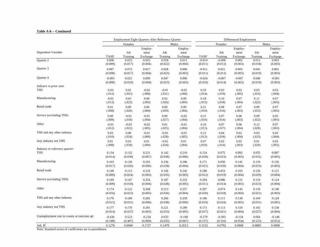
Table A-6 -- Continued

Dependent VariableTANF

Job Training

Employ-ment

ExchangeJob

Training

Employ-ment

Exchange TANF Job

Training

Employ-ment

ExchangeJob

Training

Employ-ment

ExchangeQuarter 2 0.006 0.023 0.025 0.018 0.011 -0.014 -0.006 0.002 0.012 0.003

(0.009) (0.017) (0.004) (0.022) (0.004) (0.011) (0.013) (0.003) (0.018) (0.003)Quarter 3 0.007 0.072 0.017 0.028 0.006 -0.011 0.021 0.005 0.041 0.001

(0.008) (0.017) (0.004) (0.023) (0.003) (0.011) (0.013) (0.003) (0.019) (0.003)Quarter 4 -0.003 0.022 0.009 0.047 0.006 -0.024 -0.007 -0.007 0.040 -0.001

(0.008) (0.018) (0.004) (0.023) (0.003) (0.010) (0.014) (0.003) (0.019) (0.003)Industry in prior yearTHS -0.01 0.01 -0.02 -0.01 -0.02 0.10 0.03 0.03 0.03 0.03

(.012) (.025) (.006) (.031) (.006) (.014) (.019) (.005) (.025) (.004)Manufacturing -0.01 0.03 0.00 0.02 0.00 0.18 0.10 0.07 0.11 0.07

(.012) (.023) (.005) (.026) (.004) (.015) (.018) (.004) (.022) (.003)Retail trade 0.01 0.00 0.00 0.00 0.00 0.21 0.08 0.07 0.09 0.07

(.008) (.020) (.004) (.029) (.004) (.010) (.016) (.003) (.023) (.003)Service (excluding THS) 0.00 -0.01 -0.01 0.00 -0.02 0.21 0.07 0.06 0.09 0.05

(.008) (.018) (.004) (.027) (.004) (.010) (.014) (.003) (.022) (.003)Other -0.01 -0.03 -0.02 0.01 -0.01 0.16 0.07 0.06 0.12 0.07

(.012) (.022) (.005) (.025) (.004) (.015) (.017) (.004) (.020) (.003)THS and any other industry 0.03 0.00 -0.01 -0.03 -0.01 0.12 0.04 0.02 0.03 0.02

(.010) (.024) (.006) (.028) (.005) (.013) (.018) (.004) (.023) (.004)Any industry not THS 0.01 0.03 0.01 -0.02 0.01 0.07 0.02 0.03 0.01 0.03

(.008) (.018) (.004) (.024) (.004) (.010) (.014) (.003) (.020) (.003)Industry in reference quarterTHS 0.134 0.132 0.221 0.142 0.210 0.154 0.075 0.092 0.055 0.087

(0.014) (0.030) (0.007) (0.038) (0.006) (0.018) (0.023) (0.005) (0.032) (0.005)Manufacturing 0.163 0.130 0.265 0.236 0.286 0.171 0.056 0.141 0.139 0.156

(0.017) (0.026) (0.006) (0.028) (0.004) (0.021) (0.020) (0.004) (0.023) (0.003)Retail trade 0.149 0.115 0.218 0.166 0.242 0.180 0.053 0.103 0.126 0.121

(0.009) (0.024) (0.005) (0.035) (0.005) (0.012) (0.019) (0.004) (0.029) (0.004)Service (excluding THS) 0.169 0.147 0.254 0.187 0.252 0.204 0.086 0.122 0.110 0.124

(0.009) (0.018) (0.004) (0.028) (0.005) (0.011) (0.014) (0.003) (0.023) (0.004)Other 0.174 0.122 0.268 0.213 0.257 0.207 0.074 0.145 0.139 0.140

(0.016) (0.023) (0.005) (0.026) (0.004) (0.020) (0.018) (0.004) (0.021) (0.003)THS and any other industry 0.176 0.188 0.281 0.266 0.258 0.186 0.111 0.138 0.169 0.124

(0.015) (0.031) (0.006) (0.038) (0.006) (0.019) (0.024) (0.005) (0.031) (0.005)Any industry not THS 0.177 0.170 0.281 0.221 0.289 0.173 0.113 0.150 0.165 0.158

(0.014) (0.027) (0.005) (0.033) (0.005) (0.017) (0.021) (0.004) (0.027) (0.004)Unemployment rate in county at outcome qtr -0.436 0.523 -0.234 0.633 -0.168 -0.270 -0.303 -0.154 0.064 -0.146

(0.189) (0.407) (0.069) (0.635) (0.067) (0.237) (0.316) (0.054) (0.523) (0.053)Adj. R2 0.1276 0.0940 0.1727 0.1478 0.2013 0.1532 0.0792 0.0868 0.0883 0.0908Note: Standard errors of coefficients are in parentheses.

Differenced EmploymentEmployment Eight Quarters After Reference QuarterFemales MalesFemales Males

No Job THSTHS and Any Other Industry

Other Employment

0.455 0.682 0.744 0.697(0.004) (0.013) (0.014) (0.005)

0.494 0.628 0.670 0.657(0.004) (0.014) (0.015) (0.005)

0 0.133 0.175 0.163(0) (0.014) (0.015) (0.006)

0 0.153 0.186 0.190(0) (0.018) (0.019) (0.008)

-0.163 -0.030 0.012 0(0.006) (0.014) (0.015) (0)

-0.190 -0.037 -0.004 0(0.008) (0.018) (0.019) (0)

Job Training0.575 0.753 0.819 0.760

(0.011) (0.027) (0.025) (0.008)

0.604 0.736 0.790 0.741(0.010) (0.028) (0.029) (0.009)

0 0.132 0.186 0.137(0) (0.030) (0.031) (0.013)

0 0.073 0.109 0.076(0) (0.023) (0.024) (0.010)

-0.137 -0.005 0.050 0(0.013) (0.029) (0.031) (0)

-0.076 -0.003 0.033 0(0.010) (0.023) (0.024) (0)

Employment Exchange0.417 0.698 0.786 0.757

(0.003) (0.006) (0.006) (0.002)

0.474 0.694 0.754 0.727(0.002) (0.006) (0.006) (0.002)

0 0.220 0.280 0.253(0) (0.007) (0.006) (0.003)

0 0.223 0.293 0.273(0) (0.008) (0.008) (0.004)

-0.253 -0.033 0.027 0(0.003) (0.007) (0.006) (0)

-0.273 -0.050 0.021 0(0.004) (0.008) (0.008) (0)

6. Impact on probability of employment based on difference-in-difference, relative to the non-THS category

6. Impact on probability of employment based on difference-in-difference, relative to the non-THS category

4. Impact on probability of employment based on difference-in-difference, relative to no job category

1. Probabilty of employment 8 quarters later

3. Impact on probability of employment, relative to no job category

Table A-7: Predicted Probabilility of Employment for THS and Other Employment in Quarter Following Program Entry in 1997

Panel A - Females

2. Probability of employment 8 quarters later controlling characteristics

1. Probabilty of employment 8 quarters later

3. Impact on probability of employment, relative to no job category

4. Impact on probability of employment based on difference-in-difference, relative to no job category

6. Impact on probability of employment based on difference-in-difference, relative to the non-THS category

TANF

1. Probabilty of employment 8 quarters later

2. Probability of employment 8 quarters later controlling characteristics

3. Impact on probability of employment, relative to no job category

4. Impact on probability of employment based on difference-in-difference, relative to no job category

2. Probability of employment 8 quarters later controlling characteristics

5. Impact on probability of employment, relative to the non-THS category

5. Impact on probability of employment, relative to the non-THS category

5. Impact on probability of employment, relative to the non-THS category

Table A-7 -- Continued

No Job THSTHS and Any Other Industry

Other Employment

0.470 0.646 0.806 0.752(0.015) (0.038) (0.030) (0.011)

0.516 0.658 0.782 0.724(0.014) (0.035) (0.034) (0.011)

0 0.142 0.266 0.207(0) (0.038) (0.038) (0.018)

0 0.055 0.168 0.134(0) (0.032) (0.031) (0.015)

-0.207 -0.065 0.059 0(0.018) (0.037) (0.036) (0)

-0.134 -0.079 0.034 0(0.015) (0.031) (0.030) (0)

Employment Exchange0.377 0.641 0.723 0.757

(0.002) (0.006) (0.006) (0.002)

0.451 0.660 0.709 0.715(0.002) (0.006) (0.005) (0.002)

0 0.209 0.258 0.264(0) (0.006) (0.006) (0.003)

0 0.087 0.124 0.140(0) (0.005) (0.005) (0.002)

-0.054 -0.006 -0.022 0(0.006) (0.006) (0.006) (0)

-0.140 -0.053 -0.016 0(0.002) (0.005) (0.005) (0)

Note: Standard errors are in parentheses.

5. Impact on probability of employment, relative to the non-THS category

4. Impact on probability of employment based on difference-in-difference, relative to no job category

4. Impact on probability of employment based on difference-in-difference, relative to no job category

1. Probabilty of employment 8 quarters later

2. Probability of employment 8 quarters later controlling characteristics

3. Impact on probability of employment, relative to no job category

Panel B - Males

6. Impact on probability of employment based on difference-in-difference, relative to the non-THS category

2. Probability of employment 8 quarters later controlling characteristics

5. Impact on probability of employment, relative to the non-THS category

1. Probabilty of employment 8 quarters later

3. Impact on probability of employment, relative to no job category

6. Impact on probability of employment based on difference-in-difference, relative to the non-THS category

Job Training

Table A-8: Multinomial Logit Estimation of Job Choice: Quarter Following Program Entry: 2001

Job in THS

Job in THS and

Other Industry

Job, but none in

THSJob in THS

Job in THS and

Other Industry

Job, but none in

THSJob in THS

Job in THS and

Other Industry

Job, but none in

THSJob in THS

Job in THS and

Other Industry

Job, but none in

THSJob in THS

Job in THS and

Other Industry

Job, but none in

THSConstant -5.622 -6.214 -1.429 -4.546 -4.181 0.242 -4.828 -4.588 -1.020 -7.703 -4.303 -0.267 -3.456 -3.458 0.069

(0.673) (0.800) (0.254) (1.207) (1.134) (0.487) (0.390) (0.392) (0.148) (1.257) (1.197) (0.561) (0.345) (0.353) (0.131)Age 0.115 0.164 0.014 0.019 0.021 -0.037 0.032 -0.006 -0.017 0.162 0.101 0.021 0.055 0.046 -0.022

(0.034) (0.044) (0.013) (0.045) (0.042) (0.018) (0.012) (0.012) (0.004) (0.050) (0.048) (0.021) (0.011) (0.012) (0.004)Age squared /100 -0.171 -0.290 -0.047 -0.021 -0.032 0.031 -0.064 -0.033 -0.001 -0.210 -0.150 -0.044 -0.095 -0.103 -0.001

(0.054) (0.071) (0.020) (0.057) (0.054) (0.023) (0.016) (0.017) (0.006) (0.065) (0.064) (0.027) (0.015) (0.016) (0.005)

0.056 0.040 0.056 0.065 0.057 -0.004 0.189 0.229 0.162 0.127 -0.036 -0.002 0.050 0.061 0.063(0.040) (0.044) (0.015) (0.080) (0.074) (0.033) (0.029) (0.029) (0.012) (0.078) (0.077) (0.036) (0.026) (0.027) (0.010)

High school degree 0.055 0.072 -0.021 0.292 0.014 0.084 -0.328 -0.525 -0.252 0.073 0.271 0.207 -0.308 -0.351 -0.021(0.114) (0.125) (0.045) (0.309) (0.271) (0.121) (0.109) (0.108) (0.042) (0.290) (0.276) (0.140) (0.088) (0.088) (0.037)

College degree 0.314 0.444 -0.100 0.075 -0.109 0.099 -0.467 -0.457 -0.201 -0.392 0.019 0.014 -0.233 -0.322 -0.159(0.342) (0.373) (0.171) (0.399) (0.409) (0.184) (0.140) (0.136) (0.056) (0.403) (0.439) (0.180) (0.134) (0.137) (0.050)

Nonwhite 0.574 0.491 0.177 0.339 0.433 0.236 0.266 0.103 -0.008 0.504 0.364 0.130 0.320 0.281 0.047(0.092) (0.101) (0.037) (0.175) (0.170) (0.077) (0.051) (0.052) (0.020) (0.184) (0.185) (0.090) (0.045) (0.046) (0.019)

1.128 1.348 1.153 1.385 2.078 1.032 0.466 1.220 0.921 1.193 1.703 0.356 0.787 1.172 0.975(0.203) (0.235) (0.080) (0.424) (0.428) (0.177) (0.130) (0.141) (0.050) (0.419) (0.443) (0.212) (0.115) (0.120) (0.045)

-0.019 0.401 0.154 -0.466 -0.446 -0.193 0.021 0.043 0.258 -0.004 0.407 0.145 0.186 0.391 0.327(0.111) (0.118) (0.048) (0.207) (0.194) (0.091) (0.072) (0.071) (0.027) (0.219) (0.218) (0.106) (0.067) (0.066) (0.025)

-0.253 0.003 0.011 -0.035 0.122 0.270 -0.435 -0.079 -0.437 -0.457 -0.161 -0.067 -0.383 -0.211 -0.321(0.170) (0.207) (0.059) (0.405) (0.432) (0.150) (0.096) (0.110) (0.037) (0.397) (0.419) (0.185) (0.079) (0.086) (0.033)

0.021 0.032 0.036 0.000 0.000 0.004 -0.005 0.007 0.008 -0.036 -0.050 0.000 -0.024 -0.023 0.001(0.009) (0.008) (0.004) (0.010) (0.010) (0.003) (0.003) (0.003) (0.001) (0.010) (0.011) (0.003) (0.003) (0.003) (0.000)

-0.017 -0.010 -0.015 -0.012 -0.020 -0.006 -0.010 -0.021 -0.010 -0.012 -0.017 0.000 -0.018 -0.021 -0.002(0.008) (0.008) (0.003) (0.010) (0.010) (0.004) (0.003) (0.003) (0.001) (0.009) (0.010) (0.003) (0.003) (0.003) (0.000)

Females MalesTANF Employment ExchangeJob Training

Years of education

Proportion of previous 8 quarters working

Working all of previous 8 quarters

No work in any of previous 8 quarters

Employment ExchangeJob Training

Total annual earnings in the prior year /1000Total annual earnings two years prior /1000

Table A-8 -- Continued

Job in THS

Job in THS and

Other Industry

Job, but none in

THSJob in THS

Job in THS and

Other Industry

Job, but none in

THSJob in THS

Job in THS and

Other Industry

Job, but none in

THSJob in THS

Job in THS and

Other Industry

Job, but none in

THSJob in THS

Job in THS and

Other Industry

Job, but none in

THSSt. Louis central 0.527 0.384 -0.061 1.322 0.791 0.160 0.808 0.622 -0.254 0.831 0.872 0.142 0.623 0.478 -0.217

(0.115) (0.126) (0.044) (0.225) (0.207) (0.089) (0.064) (0.065) (0.023) (0.237) (0.230) (0.104) (0.056) (0.059) (0.021)Kansas City central 0.588 0.471 -0.181 1.024 0.639 0.129 0.832 0.855 -0.203 0.643 0.668 0.049 0.717 0.787 -0.013

(0.117) (0.129) (0.047) (0.256) (0.237) (0.105) (0.072) (0.070) (0.028) (0.262) (0.255) (0.113) (0.061) (0.062) (0.024)Suburban metro 0.249 0.411 -0.218 0.450 0.759 0.336 0.737 0.510 -0.078 0.758 0.761 0.143 0.597 0.778 0.107

(0.142) (0.145) (0.052) (0.295) (0.239) (0.103) (0.070) (0.071) (0.025) (0.310) (0.301) (0.126) (0.065) (0.064) (0.023)

0.248 0.243 0.040 0.386 0.558 0.257 0.484 0.570 0.053 0.429 0.611 -0.135 0.541 0.758 0.070(0.140) (0.151) (0.049) (0.301) (0.246) (0.102) (0.079) (0.075) (0.027) (0.320) (0.294) (0.129) (0.065) (0.063) (0.024)

-0.025 -0.220 0.034 -0.310 -0.027 0.090 -0.137 -0.211 0.024 0.177 -0.206 -0.150 -0.115 -0.091 -0.085(0.095) (0.102) (0.041) (0.197) (0.171) (0.085) (0.060) (0.059) (0.023) (0.198) (0.191) (0.099) (0.055) (0.052) (0.021)

-0.305 -0.353 0.020 -0.557 -0.487 -0.064 -0.271 -0.335 -0.111 -0.286 -0.603 -0.375 -0.222 -0.352 -0.224(0.099) (0.102) (0.040) (0.188) (0.173) (0.078) (0.060) (0.059) (0.023) (0.200) (0.192) (0.092) (0.054) (0.054) (0.021)

-0.464 -0.930 -0.210 -0.314 -0.794 -0.337 -0.289 -0.527 -0.361 -0.364 -0.897 -0.429 -0.296 -0.642 -0.459(0.110) (0.127) (0.044) (0.206) (0.218) (0.091) (0.066) (0.068) (0.025) (0.228) (0.231) (0.106) (0.058) (0.061) (0.022)

-9.917 -9.014 -3.586 -7.036 -7.084 3.816 -6.941 -8.420 -2.045 10.365 6.578 5.174 -2.991 -1.752 -1.599(3.084) (3.453) (1.109) (6.086) (6.004) (2.520) (1.890) (2.023) (0.546) (6.228) (6.268) (3.082) (1.548) (1.640) (0.515)

Note: Standard errors of coefficients are in parentheses.

MalesTANF Job Training Employment Exchange Job Training Employment Exchange

Quarter 3

Quarter 4

Unemployment rate in county at current qtr

Small metro

Quarter 2

Females

Difference-in-Difference Estimates, Relative to No Job No Job THS Manufacturing Retail Trade Service1 OtherTHS and Any Other Industry

Any IndustryNot THS

TANF 0 437 756 401 679 813 734 644

(0) (69) (94) (39) (36) (72) (75) (64)

Job Training0 428 711 511 875 1,236 1,056 1,094

(0) (217) (181) (154) (117) (165) (206) (174)

Employment Exchange

0 1,339 2,097 1,270 1,723 1,947 1,847 1,899(0) (79) (59) (46) (39) (50) (79) (54)

Job Training

0 597 1,646 942 794 1,508 1,607 1,556(0) (324) (231) (271) (238) (225) (317) (279)

Employment Exchange

0 1,458 2,635 1,825 2,118 2,351 1,815 2,302(0) (117) (72) (76) (76) (63) (117) (85)

1Excluding THS.Note: Standard errors are in parentheses.

Impact on earnings

Impact on earnings

Panel B - Males

Impact on earnings

Impact on earnings

Impact on earnings

Table A-9: Predicted Earnings and Impact by Industry of Employment in Quarter Following Program Entry in 2001: Difference-in-Difference EstimatesOne Industry Multiple Industries

Panel A - Females

No Job THSTHS and Any Other Industry

Other Employment

TANF 0 1,158 1,897 1,601

(0) (43) (55) (15)767 1,488 1,900 1,557(13) (67) (80) (19)

879 1,322 1,633 1,449(15) (54) (59) (16)

0 443 754 570(0) (56) (61) (22)

0 428 725 594(0) (69) (75) (27)

-570 -128 184 0(22) (57) (61) (0)-594 -166 131 0(27) (69) (75) (0)

Job Training0 1,711 2,523 2,701

(0) (114) (103) (51)1,914 2,593 2,928 2,899

(51) (173) (166) (51)

1,927 2,525 2,943 2,894(52) (153) (143) (43)

0 597 1,016 966(0) (162) (154) (68)

0 422 1,048 869(0) (217) (206) (91)

-966 -369 49 0(68) (159) (149) (0)

-869 -447 179 0(91) (213) (200) (0)

Employment Exchange0 2,246 3,105 3,529

(0) (44) (51) (17)

1,408 2,818 3,327 3,441(16) (63) (64) (16)

1,644 2,926 3,335 3,290(17) (58) (57) (13)

0 1,282 1,691 1,646(0) (60) (60) (22)

0 1,336 1,846 1,731(0) (79) (79) (29)

-1,646 -363 45 0(22) (59) (59) (0)

-1,731 -395 115 0(29) (78) (77) (0)

1. Initial mean earnings

2. Mean earnings 8 quarters later

6. Impact on earnings, relative to the non-THS category

7. Impact on earnings based on difference-in-difference, relative to the non-THS Category

4. Impact on earnings, relative to no job category

4. Impact on earnings, relative to no job category

5. Impact on earnings based on difference-in-difference, relative to no job category

5. Impact on earnings based on difference-in-difference, relative to no job category

4. Impact on earnings, relative to no job category

3. Mean earnings 8 quarters later controlling characteristics

7. Impact on earnings based on difference-in-difference, relative to the non-THS Category

6. Impact on earnings, relative to the non-THS category

6. Impact on earnings, relative to the non-THS category

7. Impact on earnings based on difference-in-difference, relative to the non-THS Category

5. Impact on earnings based on difference-in-difference, relative to no job category

Table A-10: Predicted Earnings and Impact for THS and Other Employment in Quarter Following Program Entry in 2001

1. Initial mean earnings

2. Mean earnings 8 quarters later

Panel A - Females

3. Mean earnings 8 quarters later controlling characteristics

1. Initial mean earnings

2. Mean earnings 8 quarters later

3. Mean earnings 8 quarters later controlling characteristics

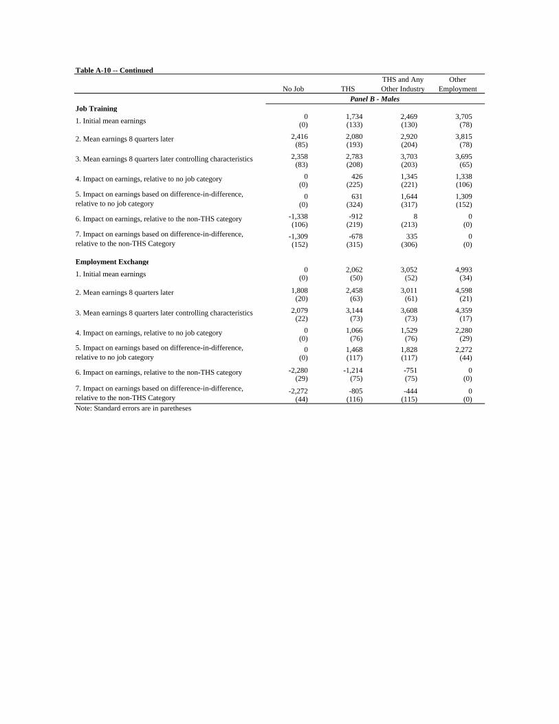
Table A-10 -- Continued

No Job THSTHS and Any Other Industry

Other Employment

Job Training0 1,734 2,469 3,705

(0) (133) (130) (78)2,416 2,080 2,920 3,815

(85) (193) (204) (78)2,358 2,783 3,703 3,695

(83) (208) (203) (65)0 426 1,345 1,338

(0) (225) (221) (106)0 631 1,644 1,309

(0) (324) (317) (152)-1,338 -912 8 0(106) (219) (213) (0)

-1,309 -678 335 0(152) (315) (306) (0)

Employment Exchange0 2,062 3,052 4,993

(0) (50) (52) (34)

1,808 2,458 3,011 4,598(20) (63) (61) (21)

2,079 3,144 3,608 4,359(22) (73) (73) (17)

0 1,066 1,529 2,280(0) (76) (76) (29)

0 1,468 1,828 2,272(0) (117) (117) (44)

-2,280 -1,214 -751 0(29) (75) (75) (0)

-2,272 -805 -444 0(44) (116) (115) (0)

Note: Standard errors are in paretheses.

5. Impact on earnings based on difference-in-difference, relative to no job category

5. Impact on earnings based on difference-in-difference, relative to no job category

1. Initial mean earnings

2. Mean earnings 8 quarters later

3. Mean earnings 8 quarters later controlling characteristics

4. Impact on earnings, relative to no job category

1. Initial mean earnings

2. Mean earnings 8 quarters later

4. Impact on earnings, relative to no job category

6. Impact on earnings, relative to the non-THS category

3. Mean earnings 8 quarters later controlling characteristics

Panel B - Males

7. Impact on earnings based on difference-in-difference, relative to the non-THS Category

6. Impact on earnings, relative to the non-THS category

7. Impact on earnings based on difference-in-difference, relative to the non-THS Category

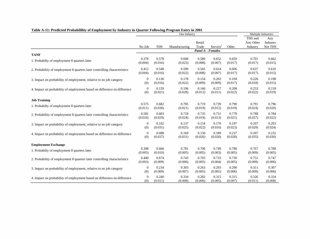
No Job THS ManufacturingRetail Trade Service1 Other

THS and Any Other Industry

Any Industry Not THS

TANF0.378 0.578 0.608 0.589 0.652 0.659 0.701 0.662

(0.004) (0.016) (0.023) (0.008) (0.007) (0.017) (0.017) (0.015)

0.412 0.548 0.590 0.565 0.614 0.606 0.637 0.610(0.004) (0.016) (0.022) (0.008) (0.007) (0.017) (0.017) (0.015)

0 0.136 0.178 0.154 0.202 0.194 0.226 0.198(0) (0.016) (0.022) (0.009) (0.009) (0.017) (0.018) (0.015)

0 0.159 0.196 0.166 0.227 0.208 0.233 0.218(0) (0.021) (0.028) (0.012) (0.011) (0.022) (0.022) (0.019)

Job Training0.575 0.682 0.785 0.719 0.739 0.790 0.791 0.796

(0.011) (0.030) (0.021) (0.019) (0.012) (0.019) (0.024) (0.020)

0.581 0.683 0.718 0.735 0.751 0.778 0.788 0.784(0.010) (0.029) (0.024) (0.019) (0.013) (0.021) (0.027) (0.022)

0 0.102 0.137 0.154 0.170 0.197 0.207 0.203(0) (0.031) (0.025) (0.022) (0.016) (0.023) (0.029) (0.024)

0 0.088 0.169 0.150 0.189 0.237 0.207 0.232(0) (0.037) (0.031) (0.026) (0.020) (0.028) (0.035) (0.030)

Employment Exchange0.398 0.666 0.781 0.706 0.749 0.780 0.767 0.788

(0.003) (0.010) (0.005) (0.005) (0.003) (0.005) (0.009) (0.005)0.440 0.674 0.743 0.703 0.733 0.730 0.751 0.747

(0.003) (0.009) (0.006) (0.005) (0.004) (0.005) (0.009) (0.006)

0 0.234 0.303 0.263 0.293 0.290 0.311 0.307(0) (0.009) (0.007) (0.005) (0.005) (0.006) (0.009) (0.006)

0 0.240 0.334 0.282 0.315 0.315 0.326 0.334(0) (0.011) (0.008) (0.006) (0.005) (0.007) (0.011) (0.008)

One Industry Multiple Industries

Panel A - Females

1. Probabilty of employment 8 quarters later

2. Probability of employment 8 quarters later controlling characteristics

1. Probabilty of employment 8 quarters later

2. Probability of employment 8 quarters later controlling characteristics

3. Impact on probability of employment, relative to no job category

3. Impact on probability of employment, relative to no job category

4. Impact on probability of employment based on difference-in-difference

2. Probability of employment 8 quarters later controlling characteristics

3. Impact on probability of employment, relative to no job category

4. Impact on probability of employment based on difference-in-difference

Table A-11: Predicted Probabilility of Employment by Industry in Quarter Following Program Entry in 2001

4. Impact on probability of employment based on difference-in-difference

1. Probabilty of employment 8 quarters later

No Job THS ManufacturingRetail Trade Service1 Other

THS and Any Other Industry

Any Industry Not THS

Job Training0.520 0.595 0.798 0.679 0.701 0.706 0.750 0.784

(0.013) (0.032) (0.017) (0.025) (0.020) (0.019) (0.028) (0.023)

0.524 0.637 0.725 0.691 0.732 0.713 0.779 0.769(0.012) (0.030) (0.020) (0.024) (0.020) (0.019) (0.029) (0.025)

0 0.113 0.202 0.168 0.208 0.189 0.255 0.245(0) (0.032) (0.023) (0.027) (0.024) (0.022) (0.032) (0.028)

0 0.115 0.225 0.152 0.185 0.217 0.232 0.259(0) (0.039) (0.028) (0.032) (0.028) (0.027) (0.038) (0.033)

Employment Exchange

0.367 0.580 0.784 0.706 0.726 0.724 0.691 0.770(0.003) (0.009) (0.004) (0.005) (0.005) (0.004) (0.008) (0.005)

0.413 0.609 0.738 0.685 0.709 0.698 0.694 0.729(0.002) (0.008) (0.004) (0.005) (0.005) (0.004) (0.008) (0.006)

0 0.196 0.325 0.272 0.296 0.285 0.281 0.316(0) (0.009) (0.005) (0.005) (0.005) (0.005) (0.008) (0.006)

0 0.193 0.340 0.284 0.301 0.289 0.282 0.322(0) (0.010) (0.006) (0.006) (0.006) (0.005) (0.010) (0.007)

1Excluding THS.Note: Standard errors are in parentheses.

Multiple IndustriesOne Industry

Panel B - Males

4. Impact on probability of employment based on difference-in-difference

2. Probability of employment 8 quarters later controlling characteristics

3. Impact on probability of employment, relative to no job category

4. Impact on probability of employment based on difference-in-difference

1. Probabilty of employment 8 quarters later

1. Probabilty of employment 8 quarters later

2. Probability of employment 8 quarters later controlling characteristics

3. Impact on probability of employment, relative to no job category

Table A-11 -- Continued

No Job THSTHS and Any Other Industry

Other Employment

TANF 0.378 0.578 0.701 0.630

(0.004) (0.016) (0.017) (0.005)

0.412 0.547 0.636 0.595(0.004) (0.016) (0.017) (0.005)

0 0.135 0.224 0.183(0) (0.016) (0.018) (0.007)

0 0.157 0.231 0.202(0) (0.021) (0.022) (0.008)

-0.183 -0.048 0.041 0(0.007) (0.017) (0.018) (0)

-0.202 -0.045 0.029 0(0.008) (0.021) (0.022) (0)

Job Training0.575 0.682 0.791 0.756

(0.011) (0.030) (0.024) (0.008)

0.581 0.683 0.787 0.752(0.010) (0.029) (0.027) (0.008)

0 0.101 0.206 0.171(0) (0.031) (0.029) (0.013)

0 0.087 0.206 0.192(0) (0.037) (0.035) (0.016)

-0.171 -0.070 0.035 0(0.013) (0.030) (0.028) (0)

-0.192 -0.105 0.014 0(0.016) (0.036) (0.034) (0)

Employment Exchange0.398 0.666 0.767 0.755

(0.003) (0.010) (0.009) (0.002)

0.440 0.674 0.751 0.729(0.003) (0.009) (0.009) (0.002)

0 0.234 0.310 0.289(0) (0.009) (0.009) (0.003)

0 0.239 0.326 0.312(0) (0.011) (0.011) (0.004)

-0.289 -0.055 0.021 0(0.003) (0.009) (0.009) (0)

-0.312 -0.073 0.014 0(0.004) (0.011) (0.011) (0)

Table A-12: Predicted Probabilility of Employment for THS and Other Employment in Quarter Following Program Entry in 2001

Panel A - Females

2. Probability of employment 8 quarters later controlling characteristics

1. Probabilty of employment 8 quarters later

2. Probability of employment 8 quarters later controlling characteristics

3. Impact on probability of employment, relative to no job category

4. Impact on probability of employment based on difference-in-difference, relative to no job category

4. Impact on probability of employment based on difference-in-difference, relative to no job category

1. Probabilty of employment 8 quarters later

5. Impact on probability of employment, relative to the non-THS category

6. Impact on probability of employment based on difference-in-difference, relative to the non-THS category

1. Probabilty of employment 8 quarters later

5. Impact on probability of employment, relative to the non-THS category

2. Probability of employment 8 quarters later controlling characteristics

6. Impact on probability of employment based on difference-in-difference, relative to the non-THS category

5. Impact on probability of employment, relative to the non-THS category

6. Impact on probability of employment based on difference-in-difference, relative to the non-THS category

3. Impact on probability of employment, relative to no job category

3. Impact on probability of employment, relative to no job category

4. Impact on probability of employment based on difference-in-difference, relative to no job category

No Job THSTHS and Any Other Industry

Other Employment

Job Training0.520 0.595 0.750 0.734

(0.013) (0.032) (0.028) (0.009)

0.524 0.636 0.778 0.725(0.012) (0.030) (0.029) (0.009)

0 0.112 0.254 0.201(0) (0.032) (0.032) (0.015)

0 0.116 0.234 0.208(0) (0.039) (0.038) (0.018)

-0.201 -0.088 0.053 0(0.015) (0.031) (0.030) (0)

-0.208 -0.092 0.026 0(0.018) (0.037) (0.036) (0)

Employment Exchange0.367 0.580 0.691 0.742

(0.003) (0.009) (0.008) (0.002)

0.414 0.610 0.695 0.711(0.002) (0.008) (0.008) (0.002)

0 0.196 0.281 0.297(0) (0.009) (0.008) (0.003)

0 0.193 0.282 0.305(0) (0.010) (0.010) (0.004)

-0.297 -0.101 -0.016 0(0.003) (0.008) (0.008) (0)

-0.305 -0.113 -0.024 0(0.004) (0.010) (0.010) (0)

Note: Standard errors are in parentheses.

6. Impact on probability of employment based on difference-in-difference, relative to the non-THS category

5. Impact on probability of employment, relative to the non-THS category

6. Impact on probability of employment based on difference-in-difference, relative to the non-THS category

2. Probability of employment 8 quarters later controlling characteristics

5. Impact on probability of employment, relative to the non-THS category

1. Probabilty of employment 8 quarters later

3. Impact on probability of employment, relative to no job category

4. Impact on probability of employment based on difference-in-difference, relative to no job category

4. Impact on probability of employment based on difference-in-difference, relative to no job category

1. Probabilty of employment 8 quarters later

2. Probability of employment 8 quarters later controlling characteristics

3. Impact on probability of employment, relative to no job category

Panel B - Males

Table A-12 -- Continued

Table A-13: Transition between Sectors Over Eight Quarters: 2001

Reference Quarter Employment No Job

Service, including temp help Manufacturing

Retail trade Other

Multiple sectors Total

TANF No job 62.2 16.7 1.8 10.3 4.9 4.2 100.0One THS 42.2 26.5 4.4 8.6 10.7 7.6 100.0

Sector Manufacturing 39.2 13.3 22.5 10.9 6.4 7.7 100.0Retail trade 41.1 15.5 1.8 28.2 5.6 7.8 100.0Service1 34.8 41.5 1.5 8.6 5.8 7.7 100.0Other 34.1 15.9 1.6 9.6 31.6 7.3 100.0

Multiple THS and any other industry 29.9 30.3 2.5 13.5 9.5 14.3 100.0Sectors Any industry not THS 33.8 23.5 2.8 17.6 9.6 12.8 100.0

Job Training No job 42.5 26.6 6.6 8.2 11.0 5.1 100.0One THS 31.8 32.6 9.1 7.0 14.5 5.0 100.0

Sector Manufacturing 21.5 16.8 42.8 7.2 7.5 4.3 100.0Retail trade 28.1 16.3 3.1 35.1 8.0 9.4 100.0Service1 26.1 50.2 1.7 4.0 9.2 8.8 100.0Other 21.0 14.5 3.3 5.6 49.1 6.5 100.0

Multiple THS and any other industry 20.9 27.7 10.1 10.4 17.6 13.3 100.0Sectors Any industry not THS 20.5 29.9 6.7 11.5 16.7 14.7 100.0

Employment Exchange No job 60.2 16.5 2.9 8.5 8.8 3.2 100.0 100

One THS 33.4 28.4 5.5 8.0 17.9 6.8 100.0Sector Manufacturing 21.9 7.7 56.2 3.9 5.8 4.6 100.0

Retail trade 29.4 13.9 2.3 38.4 8.4 7.6 100.0Service1 25.1 54.0 1.4 5.4 7.7 6.4 100.0Other 22.0 11.6 3.6 4.8 52.4 5.5 100.0

Multiple THS and any other industry 23.3 29.4 7.7 11.1 17.6 10.9 100.0Sectors Any industry not THS 21.2 25.7 6.9 12.7 18.9 14.6 100.0

Job Training No job 48.0 13.4 10.1 6.7 17.4 4.5 100.0

One THS 40.5 21.5 10.1 4.2 15.6 8.0 100.0Sector Manufacturing 20.2 8.6 48.1 5.0 14.1 3.9 100.0

Retail trade 32.1 7.9 6.8 31.6 10.7 11.0 100.0Service1 29.9 37.1 3.6 7.6 14.9 7.0 100.0Other 29.4 9.0 5.3 2.3 48.7 5.3 100.0

Multiple THS and any other industry 25.0 22.6 11.7 9.7 17.7 13.3 100.0Sectors Any industry not THS 21.7 15.6 14.6 11.9 22.9 13.4 100.0

Employment Exchange No job 63.3 8.9 5.4 6.2 13.4 2.9 100.0

One THS 42.0 17.2 10.9 7.4 15.3 7.2 100.0Sector Manufacturing 21.6 4.5 58.5 3.0 8.2 4.2 100.0

Retail trade 29.4 8.1 4.3 39.8 10.8 7.6 100.0Service1 27.4 45.2 3.3 6.1 11.6 6.4 100.0Other 27.6 5.7 4.5 3.6 54.1 4.6 100.0

Multiple THS and any other industry 30.9 16.0 12.7 9.6 19.2 11.6 100.0Sectors Any industry not THS 23.0 14.7 11.6 13.1 23.6 14.1 100.0

1Excluding THS.

Employment Eight Quarters Later

Panel A - Females

Panel B - Males

Impacts Relative to No Job THS Manufacturing Retail Trade Service1 Other

THS and Any Other

Industry

Any Industry Not

THS

TANF 155 277 86 180 312 298 171(42) (58) (24) (23) (45) (46) (39)

1059 2968 1749 2293 2837 1810 2192(55) (54) (25) (22) (33) (58) (39)

Job Training277 337 122 364 541 302 384

(123) (106) (89) (67) (97) (116) (99)

1878 4396 2574 3300 3767 2785 3426(161) (104) (90) (64) (80) (190) (109)

Employment Exchange414 455 305 484 596 464 531(47) (39) (28) (24) (31) (47) (33)

2472 4922 2997 3727 4441 3004 3954(67) (37) (28) (23) (27) (77) (39)

Table A-14: Predicted Earnings and Impact by Employment in Reference and Outcome Quarter: 2001

1. Impact of reference quarter industry, controlling outcome industry

One Industry Multiple Industries

Panel A - Females

1. Impact of reference quarter industry, controlling outcome industry

1. Impact of reference quarter industry, controlling outcome industry

2. Impact of outcome quarter industry, controlling reference quarter industry

2. Impact of outcome quarter industry, controlling reference quarter industry

2. Impact of outcome quarter industry, controlling reference quarter industry

Impacts Relative to No Job THS Manufacturing Retail Trade Service1 Other

THS and Any Other

Industry

Any Industry Not

THS

Job Training13 352 234 218 563 319 468

(167) (125) (143) (125) (119) (165) (145)

2421 5879 3555 4010 4809 2819 4451(203) (127) (143) (123) (104) (243) (182)

Employment Exchange135 620 506 548 730 92 626(61) (40) (40) (41) (34) (61) (45)

2586 6354 4232 5004 5768 3406 5096(82) (39) (40) (39) (31) (91) (54)

1Excluding THS.Note: Standard errors are in parentheses.

Table A-14 -- ContinuedOne Industry Multiple Industries

1. Impact of reference quarter industry, controlling outcome industry2. Impact of outcome quarter industry, controlling reference quarter industry

1. Impact of reference quarter industry, controlling outcome industry

2. Impact of outcome quarter industry, controlling reference quarter industry

Panel B - Males