The Role of Spike Patterns in Neuronal Information Processing
264
DISS. ETH NO. 16464 The Role of Spike Patterns in Neuronal Information Processing A Historically Embedded Conceptual Clarification A dissertation submitted to the SWISS FEDERAL INSTITUTE OF TECHNOLOGY ZURICH for the degree of Doctor of Sciences (Dr. sc. ETH Z¨ urich) presented by Markus Christen Lic. phil. nat., Universit¨ at Bern born 07. 01. 1969 accepted on the recommendation of Prof. Dr. Rodney Douglas, Examiner PD Dr. Ruedi Stoop, Co-Examiner, Supervisor Prof. Dr. Michael Hagner, Co-Examiner 2006
Transcript of The Role of Spike Patterns in Neuronal Information Processing

DISS. ETH NO. 16464
The Role of Spike Patternsin Neuronal Information Processing
A Historically Embedded
Conceptual Clarification
A dissertation submitted to the
SWISS FEDERAL INSTITUTE OF TECHNOLOGY ZURICH
for the degree of
Doctor of Sciences (Dr. sc. ETH Zurich)
presented by
Markus ChristenLic. phil. nat., Universitat Bern
born 07. 01. 1969
accepted on the recommendation of
Prof. Dr. Rodney Douglas, ExaminerPD Dr. Ruedi Stoop, Co-Examiner, Supervisor
Prof. Dr. Michael Hagner, Co-Examiner
2006

ii
Author:Markus Christen, lic. phil. nat.Institute of NeuroinformaticsWinterthurerstrasse 190
8057 Zurich
c© 2006 BrainformBozingenstrasse 5, 2502 Biel, Switzerlandhttp://www.brainform.com
Print: Printy, Theresienstrasse 69, 80333 MunchenPrinted in Germany
ISBN-10: 3-905412-00-4ISBN-13: 978-3-905412-00-4
Purchase order: [email protected]
This work is subject to copyright. All rights are reserved, whether the whole or part of the mate-
rial is concerned, specifically the rights of translation, reprinting, reuse of illustrations, recitation,
broadcasting, reproduction on microfilm or in any other way, and storage in data banks. Duplica-
tion of this publication or parts thereof is permitted only with prior permission from the current
publishers. No part of this publication may be stored in a retrieval system, or transmitted in any
form or by any means, electronic, mechanical, photocopying, recording or otherwise, without prior
permission from the publishers. You are not allowed to modify, amend or otherwise change this
work without prior consent from the the current publishers. All copyright for this work will remain
the property of the author.
Acknowledgements
Writing a PhD thesis is embedded in a net of relations and conditions. Therefore, I havemany thanks to express. First, I’m indebted to my PhD supervisor, PD Dr. Ruedi Stoop.He not only made it possible for me to re-enter science after a longer stay in professionallife. He also is convinced of the idea that one should find one’s own topic instead of beingassigned to one. He offered help, when it was important, and recalcitrance, when it wasnecessary in order to sharpen my own ideas. He finally allowed my expeditions into thefields of humanities, which made it possible to combine two cultures in this interdisciplinaryPhD, which usually remain separated. Profs. David Gugerli and Michael Hagner werethe exponents on the other side of this cultural divide, who provided assistance and manyhelpful comments. Sincere thanks go to both of them.
I was lucky that I was integrated in a small, but busy group of excellent physicists andengineers. We not only shared science, but also life and beer to some degree – an aspect thatnever should be underestimated. Specific thanks go to Albert Kern for his assistance inunderstanding the correlation integral, to Thomas Ott for many clusterings and to Jan-
Jan van der Vyver for programming, computer, and language help. Various alumni andvisitors of the Stoop group and many more people in the Institute of Neuroinformaticscould be mentioned as well. I cut short by thanking Profs. Rodney Douglas and Kevan
Martin, who made it possible that such an institute can exist. Furthermore, I’m verymuch obliged to those, who provided data that have been used in this study and made itpossible to analyze the tools introduced by this work. My thanks go to Alister Nicol
of the Cognitive & Behavioural Neuroscience Lab of the Babraham Institute in Cambridge,Adam Kohn of the Center of Neural Science of the New York University, Valerio Mante
and Matteo Carandini of the Smith Kettlewell Eye Research Institute in San Francisco,and Kevan Martin of the Institute of Neuroinformatics.
The historical part of this PhD originated in the Max Planck Institute for the History ofScience in Berlin. Many thanks go to Profs. Michael Hagner and Hans-Jorg Rhein-
berger, who made it possible to join this exciting community from December 2004 to March2005. I also thank Urs Schoepflin for his helpful comments for my bibliometric studiesand the participants of the colloquium of the ‘Abteilung III’ that commented and criticizedthe first version of this part. I finally thank Robert Ruprecht and Adrian Whatley
for proofreading the scientific and the historical part of this thesis. They are certainly notto blame for the remaining mistakes. The most important thanks are always expressed atthe end: I thank my parents and my sisters for their existence, and Meret for her love.
Markus Christen, November 2005
iii

iv

Contents
Acknowledgements iii
Zusammenfassung ix
Summary x
Statement xii
1 Introductory Remarks 11.1 Goals of this Study . . . . . . . . . . . . . . . . . . . . . . . . . . . . . . . . . 11.2 Methodology . . . . . . . . . . . . . . . . . . . . . . . . . . . . . . . . . . . . 31.3 Organization of the Thesis . . . . . . . . . . . . . . . . . . . . . . . . . . . . . 3
1.3.1 Main Line of Argumentation . . . . . . . . . . . . . . . . . . . . . . . 31.3.2 Typographic Structure and Layout . . . . . . . . . . . . . . . . . . . . 5
1.4 Abbreviations and List of Symbols . . . . . . . . . . . . . . . . . . . . . . . . 61.4.1 Abbreviations . . . . . . . . . . . . . . . . . . . . . . . . . . . . . . . . 61.4.2 List of Symbols . . . . . . . . . . . . . . . . . . . . . . . . . . . . . . . 6
I Historical Roots of the Information Processing Brain 9
2 The Brain on the Cusp of the Information Age 112.1 Introduction . . . . . . . . . . . . . . . . . . . . . . . . . . . . . . . . . . . . . 11
2.1.1 The Information Processing Brain . . . . . . . . . . . . . . . . . . . . 112.1.2 The Historical Context . . . . . . . . . . . . . . . . . . . . . . . . . . . 13
2.2 Cornerstones of the Information Age . . . . . . . . . . . . . . . . . . . . . . . 152.2.1 The Conceptualization of Information . . . . . . . . . . . . . . . . . . 152.2.2 Information Theory . . . . . . . . . . . . . . . . . . . . . . . . . . . . 162.2.3 Cybernetics . . . . . . . . . . . . . . . . . . . . . . . . . . . . . . . . . 19
2.3 Preconditions for the Information Processing Brain . . . . . . . . . . . . . . . 212.3.1 The Scheme for Analysis . . . . . . . . . . . . . . . . . . . . . . . . . . 212.3.2 The Neuron Doctrine . . . . . . . . . . . . . . . . . . . . . . . . . . . 232.3.3 Spikes and Messages . . . . . . . . . . . . . . . . . . . . . . . . . . . . 252.3.4 Measuring Single Fibres . . . . . . . . . . . . . . . . . . . . . . . . . . 28
v

vi CONTENTS
3 The Birth of the Information Processing Brain 313.1 1940-1970: Overview . . . . . . . . . . . . . . . . . . . . . . . . . . . . . . . . 313.2 1940-1970: Detailed Analysis . . . . . . . . . . . . . . . . . . . . . . . . . . . 33
3.2.1 A new Role for the Neuron? . . . . . . . . . . . . . . . . . . . . . . . . 333.2.2 Applying the Information Vocabulary . . . . . . . . . . . . . . . . . . 353.2.3 The Emergence of a Toolbox for Spike Train Analysis . . . . . . . . . 513.2.4 The (Random) Network . . . . . . . . . . . . . . . . . . . . . . . . . . 533.2.5 The Active and Reliable Brain . . . . . . . . . . . . . . . . . . . . . . 563.2.6 The Modelling Approach . . . . . . . . . . . . . . . . . . . . . . . . . 61
4 1940 – 1970: The Dynamics of Research 654.1 Journals and Publications . . . . . . . . . . . . . . . . . . . . . . . . . . . . . 654.2 Conferences . . . . . . . . . . . . . . . . . . . . . . . . . . . . . . . . . . . . . 694.3 Protagonists . . . . . . . . . . . . . . . . . . . . . . . . . . . . . . . . . . . . . 754.4 Synopsis: Qualitative and Quantitative Analysis . . . . . . . . . . . . . . . . 86
4.4.1 Up to 1940: Preconditions . . . . . . . . . . . . . . . . . . . . . . . . . 864.4.2 1940-1970: Main Developments . . . . . . . . . . . . . . . . . . . . . . 88
II Patterns in Neuronal Spike Trains 91
5 Neural Coding and Computation 935.1 Neural Coding . . . . . . . . . . . . . . . . . . . . . . . . . . . . . . . . . . . 93
5.1.1 What is a ‘Neural Code’? . . . . . . . . . . . . . . . . . . . . . . . . . 935.1.2 Rate Coding vs. Temporal Coding . . . . . . . . . . . . . . . . . . . . 1005.1.3 Single Neurons vs. Neuronal Assemblies . . . . . . . . . . . . . . . . . 102
5.2 Neural Computation . . . . . . . . . . . . . . . . . . . . . . . . . . . . . . . . 103
6 Defining Patterns 1056.1 Characteristics of Patterns . . . . . . . . . . . . . . . . . . . . . . . . . . . . . 105
6.1.1 Defining ‘Spike Pattern’ . . . . . . . . . . . . . . . . . . . . . . . . . . 1056.1.2 Types of Events . . . . . . . . . . . . . . . . . . . . . . . . . . . . . . 1086.1.3 The Stability of Patterns . . . . . . . . . . . . . . . . . . . . . . . . . 111
6.2 The Background of a Pattern . . . . . . . . . . . . . . . . . . . . . . . . . . . 1136.2.1 The Significance of Patterns . . . . . . . . . . . . . . . . . . . . . . . . 1136.2.2 The Poisson Hypothesis . . . . . . . . . . . . . . . . . . . . . . . . . 1136.2.3 Randomization Methods . . . . . . . . . . . . . . . . . . . . . . . . . . 116
6.3 Noise and Reliability . . . . . . . . . . . . . . . . . . . . . . . . . . . . . . . . 1196.3.1 What is Noise in Neuronal Systems? . . . . . . . . . . . . . . . . . . . 1196.3.2 Noise Sources in Neurons . . . . . . . . . . . . . . . . . . . . . . . . . 1196.3.3 The Reliability of Neurons . . . . . . . . . . . . . . . . . . . . . . . . . 1226.3.4 Can Neurons Benefit from Noise? . . . . . . . . . . . . . . . . . . . . . 124
6.4 Functional Aspects of Spike Patterns . . . . . . . . . . . . . . . . . . . . . . . 1256.4.1 Causing Patterns: Network, Oscillation, Synchronization . . . . . . . . 1266.4.2 Using Patterns: LTP and Coincidence-Detection . . . . . . . . . . . . 131
6.5 Spike Patterns: Examples . . . . . . . . . . . . . . . . . . . . . . . . . . . . . 134

CONTENTS vii
6.6 The Stoop-Hypothesis . . . . . . . . . . . . . . . . . . . . . . . . . . . . . . . 1376.6.1 Neurons as Limit Cycles . . . . . . . . . . . . . . . . . . . . . . . . . . 1386.6.2 Locking – The Coupling of Limit Cycles . . . . . . . . . . . . . . . . . 1396.6.3 Emergence of a Coding Scheme . . . . . . . . . . . . . . . . . . . . . . 1416.6.4 The Role of Patterns . . . . . . . . . . . . . . . . . . . . . . . . . . . . 1466.6.5 The Integral Framework . . . . . . . . . . . . . . . . . . . . . . . . . . 148
7 Detecting Patterns 1517.1 The Problem of Pattern Detection . . . . . . . . . . . . . . . . . . . . . . . . 151
7.1.1 Outlining the Problem . . . . . . . . . . . . . . . . . . . . . . . . . . . 1517.1.2 Pattern Detection Methods: Overview . . . . . . . . . . . . . . . . . . 1527.1.3 Spike Train Distance Measures: Overview . . . . . . . . . . . . . . . . 153
7.2 Histogram-based Pattern Detection . . . . . . . . . . . . . . . . . . . . . . . . 1557.2.1 Classes of Histograms . . . . . . . . . . . . . . . . . . . . . . . . . . . 1557.2.2 1D Interval Histograms . . . . . . . . . . . . . . . . . . . . . . . . . . 160
7.3 Correlation Integral based Pattern Discovery . . . . . . . . . . . . . . . . . . 1637.3.1 The Correlation Integral . . . . . . . . . . . . . . . . . . . . . . . . . . 1637.3.2 Smeared log-log Steps . . . . . . . . . . . . . . . . . . . . . . . . . . . 1647.3.3 Pattern Length Estimation . . . . . . . . . . . . . . . . . . . . . . . . 166
7.4 Template-based Pattern Recognition . . . . . . . . . . . . . . . . . . . . . . . 1707.4.1 The Template Approach . . . . . . . . . . . . . . . . . . . . . . . . . . 1707.4.2 Problems with Templates . . . . . . . . . . . . . . . . . . . . . . . . . 171
7.5 Clustering-based Pattern Quantification . . . . . . . . . . . . . . . . . . . . . 1737.5.1 The Clustering Algorithm . . . . . . . . . . . . . . . . . . . . . . . . . 1737.5.2 Relating Patterns and Clusters . . . . . . . . . . . . . . . . . . . . . . 174
7.6 The LZ-Distance of Spike Trains . . . . . . . . . . . . . . . . . . . . . . . . . 1777.6.1 The LZ-Distance Measure . . . . . . . . . . . . . . . . . . . . . . . . . 1787.6.2 Assessment of the LZ-Distance . . . . . . . . . . . . . . . . . . . . . . 179
7.7 Pattern Detection: Summary . . . . . . . . . . . . . . . . . . . . . . . . . . . 183
8 Investigating Patterns 1858.1 Description of the Data . . . . . . . . . . . . . . . . . . . . . . . . . . . . . . 185
8.1.1 Rat Data: Olfactory System (mitral cells) . . . . . . . . . . . . . . . . 1858.1.2 Cat Data: Visual System (LGN, striate cortex) . . . . . . . . . . . . . 1868.1.3 Monkey Data: Visual System (LGN, V1, MT) . . . . . . . . . . . . . 186
8.2 First Prediction: Firing statistics . . . . . . . . . . . . . . . . . . . . . . . . . 1878.3 Second Prediction: Firing Reliability . . . . . . . . . . . . . . . . . . . . . . . 1898.4 Third Prediction: Neuronal Clustering . . . . . . . . . . . . . . . . . . . . . . 1928.5 Fourth Prediction: Classes of Firing . . . . . . . . . . . . . . . . . . . . . . . 1958.6 Fifth Prediction: Pattern Stability . . . . . . . . . . . . . . . . . . . . . . . . 196
9 Conclusions 1999.1 Support for the Stoop-Hypothesis . . . . . . . . . . . . . . . . . . . . . . . . . 1999.2 The Stoop-Hypothesis in the General Context . . . . . . . . . . . . . . . . . . 2019.3 Outlook: Experimental Approaches . . . . . . . . . . . . . . . . . . . . . . . . 201

viii CONTENTS
III Appendix 203
Figures 205
Tables 206
Bibliography 207
Index 241
List of Publications 245
Curriculum Vitae 247
Zusammenfassung
Es ist heutzutage ein Gemeinplatz, das Gehirn als informationsverarbeitendes System zubetrachten. Obgleich dieser Ausdruck sowohl innerhalb der Neurowissenschaft wie auchin einem weiteren Umfeld breite Verwendung findet, druckt er kein prazises Verstandnisuber die Vorgange im Nervensystem aus. Klar ist zwar, dass der Begriff nicht (mehr)eine enge Analogie zwischen klassischen Computern und dem Gehirn zum Ausdruck brin-gen soll. Heute wird vielmehr ein prinzipieller Unterschied zwischen diesen beiden Artender Informationsverarbeitung postuliert. Der Informationsbegriff der Neurowissenschaft wieauch die mit der Informationsverarbeitung verbundenen Prozesse, die oft als ein neuronalerKode (neural code) oder eine neuronale Berechnung (neural computation) aufgefasst werden,bleiben damit weiterhin Gegenstand intensiver Forschungen. Diese Forschungen benotigenklare und definierte Begriffe. Die vorliegende Arbeit will zu dieser Klarung beitragen, indemder Begriff des ‘Feuermusters’ (spike pattern) definiert und hinsichtlich seiner Anwendungim Kontext des neural coding und der neural computation dargelegt werden soll.
Diese Arbeit verbindet eine naturwissenschaftliche Analyse – welche die Begriffsklarung,eine Hypothesenbildung und die Untersuchung experimenteller Daten umfasst – mit einerwissenschafthistorischen Untersuchung. Letztere will die historischen Wurzeln der heutigenDebatten um neural coding und neural computation freilegen. Der Schwerpunkt der his-torischen Analyse liegt in den 1940er bis 1960er Jahren – jenen Jahrzehnten also, in welcheneine Verwissenschaftlichung des Informationsbegriffs im Verbund mit der aufkommendenInformationstheorie und Kybernetik stattfand, die zu einem eigentlichen ‘Informations-Vokabular’ fuhrten, mit zentralen Begriffen wie Kode (code), Berechnung (computation)und Rauschen (noise). Im historischen Teil werden zudem jene zuvor stattgefundenen Ent-wicklungen innerhalb der Neurowissenschaft skizziert, welche Voraussetzungen fur die An-wendbarkeit des ‘Informations-Vokabulars’ schufen. Wichtige Beispiele sind die Entwicklungvon Geraten fur die zuverlassige Messung des neuronalen Feuerns und die Diskussion ubermessages in solchen Messungen des neuronalen Feuerverhaltens. Danach zeigen wir anhandeines detaillierten historischen Analyse-Schemas auf, welche Entwicklungen zum Begriff des‘informationsverarbeitenden Gehirns’ beigetragen haben. Diese Untersuchung wird mit bib-liometrischen und scientometrischen Analysen erganzt, welche zur Identifikation wichtigerKonferenzen und zentraler Protagonisten des damaligen Diskurses dienen.
Auch der naturwissenschaftliche Teil beinhaltet eine Ubersicht uber einige der heutewichtigen Theorien uber die neuronale Kodierung bzw. die neuronale Informationsverar-beitung. Danach folgt eine Scharfung des Begriffs ‘Feuermuster’ anhand seiner vielfaltigenVerwendungsweisen in der wissenschaftlichen Literatur. Wir zeigen auf, dass dieser Begriffimmer zusammen mit statistischen Hypothesen uber das ‘Nicht-Muster’ verwendet wer-
ix

x CONTENTS
den muss, geben eine Ubersicht der gangigen Randomisierungsverfahren und diskutierendie Rolle des neuronal noise. Danach prasentieren wir im Detail eine von Ruedi Stoop
und Mitarbeitern entwickelte Hypothese, in welcher die verschiedenen diskutierten Aspekte– insbesondere die Feuermuster und neuronal noise – eine Verbindung eingehen. DieseStoop-Hypothese basiert auf der Feststellung, dass sich kortikale Neuronen unter quasi-stationaren Bedingungen als Grenzzyklen beschreiben lassen. Diese werden von den zahlre-ichen einkommenden synaptischen Impulsen (Hintergrund-Aktivitat, oft als eine Form vonneuronal noise aufgefasst), die sich unter der Bedingung der Quasi-Stationaritat als kon-stanten Strom auffassen lassen, getrieben. Die Kopplung solcher Grenzzyklen fuhrt zumgenerischen Phanomen der Frequenzeinrastung (locking). Damit lasst sich ein Schema neu-ronaler Kodierung erstellen, wonach sich die unterschiedliche Hintergrund-Aktivitat zweierNeuronen, die wiederum Ausdruck spezifischer sensorischer Information sind, in ein spezi-fisches Feuermuster niederschlagen.
Aufbauend auf dieser Hypothese werden funf Voraussagen abgeleitet, welche sich beider Untersuchung neuronaler Daten zeigen lassen sollten. Demnach sollte erstens nur eineMinderheit von kortikalen Neuronen eine mit dem Poisson-Modell vereinbare Feuerstatistikzeigen. Zweitens erwarten wir Unterschiede in der Zuverlassigkeit des Feuerns hinsichtlichdes timings von Nervenimpulsen und der Reproduzierbarkeit spezifischer Feuermuster jenach Ort der Messung entlang des Pfades der neuronalen Informationsverarbeitung. Drittenssollten sich in der parallelen Messung einer Vielzahl von Neuronen Gruppen von Neuronenmit ahnlichen Feuermustern finden. Viertens erwarten wir, dass eine bereits festgestellteKlassierung von Neuronen in drei Gruppen (solche mit unkorreliertem Feuern, solche mitinstabilen Feuermustern und solche mit stabilen Feuermuster) auch im von uns untersuchtenDatenset feststellbar ist. Funftens erwarten wir, dass Feuermuster, die mutmasslich Ergebniseiner neuronalen Informationsverarbeitung sind, in einem von uns definierten Sinn stabilersind als solche, die von Stimulus-Eigenschaften herruhren, die vermutlich fur den Organismuskeine Rolle spielen.
Ein zentraler Teil der Arbeit bildet eine Darstellung des Problems der Erkennung vonFeuermustern. Wir bieten dazu eine Ubersicht uber gangige Histogramm und Templatebasierende Methoden und zeigen die damit verbundenen Schwierigkeiten auf. Danach prasen-tieren wir eine Reihe neuer Methoden fur die Mustererkennung, basierend auf dem Korre-lationsintegral, dem sequenziellen superparamagnetischen Clustering-Algorithmus und derLempel-Ziv-Komplexitat. Moglichkeiten und Grenzen dieser Methoden werden im Detailvorgefuhrt und in einem allgemeinen Schema zum Problem der Mustererkennung in neu-ronalen Daten – so genannten spike trains – integriert.
Im empirischen Teil zeigen wir einerseits die Anwendbarkeit der von uns entwickel-ten Methoden auf. Andererseits konnten wir, obwohl die uns zur Verfugung gestande-nen Daten ursprunglich fur anderweitige Zwecke erhoben wurden und damit nicht op-timal waren, die genannten Hypothesen bestatigen. Dies sind wichtige Indizien fur dieGultigkeit der Stoop-Hypothese zur neuronalen Informationsverarbeitung. Eine eigentlicheexperimentelle Prufung der Hypothese war indes aufgrund externer Grunde nicht moglich.Wir zeigen deshalb auch, welche weiteren Schritte fur die Prufung der Stoop-Hypotheseangezeigt sind. In ihrer Gesamtheit soll die vorliegende Arbeit auch als Einfuhrung indie Problematik der neuronalen Informationsverarbeitung verstanden werden. Aus diesemGrund wurde auf gestalterische Fragen grossen Wert gelegt, so dass diese Arbeit dem Leserals Hilfsmittel und Nachschlagewerk dienen kann.

Summary
Today, understanding the brain as a ‘information processing device’ is a commonplace. Al-though this expression is widely used within and outside of neuroscience, it does not reallyexpress a precise understanding of the neuronal processes. However, it is clear that the‘information processing brain’ does no longer express a close relationship between classical(digital) computers and the brain. Rather, a clear distinction between these two modesof information processing is postulated. Nevertheless, the concept of information in neuro-science, as well as the related concepts of neural coding and neural computation, are still atopic of intensive research within neuroscience. This also requires some clarification on theconceptual level. This PhD thesis intends to contribute to this clarification by defining theterm ‘spike pattern’ and by evaluating the application of this concept within the frameworkof neural coding and neural computation.
This thesis unifies a scientific analysis – including a conceptual clarification, the formu-lation of a hypothesis and data analysis – with a historical investigation. The latter intendsto analyze the historical roots of today’s discussion on neural coding and neural compu-tation. The focus of the historical analysis lies in the period of the 1940s to 1960s – thedecades in which a scientific conceptualization of information in relation to the emerginginformation theory and cybernetics is observed. This led to the formation of a ‘informationvocabulary’, whose central terms are ‘code’, ‘computation’ and ‘noise’. Furthermore, in thehistorical part, those development within the history of neuroscience before this period thatformed the preconditions for the application of this vocabulary will be sketched. Importantexamples are the construction of measurement devices that allowed the reliable recording ofneuronal firing, and the discussion about ‘messages’ in neuronal data. Then we show, usinga detailed scheme of analysis, which specific developments led to the formation of the notionof a ‘information processing brain’. This investigation is accompanied by several bibliomet-ric and scientometric studies, which lead to the identification of important conferences andprotagonists during this period.
The scientific part also includes a review of some current theories of neural coding andneural information processing. This will be followed by a sharpening of the concept of‘spike pattern’, referring to its current use in the neuroscience literature. We show thatthis concept always involves a clear statistical hypothesis of a ‘non-pattern’, we provide aoverview of the common randomization methods for spike data and we discuss the role ofneuronal noise. Then we present a hypothesis, developed by Ruedi Stoop and co-workers(Stoop-hypothesis), in which the discussed concept – notably spike patterns and noise – canbe put in a common context. The Stoop-hypothesis is based on the finding that corticalneurons under quasi-stationary conditions can be described as limit cycles. They are driven
xi

xii CONTENTS
by the numerous incoming synaptic impulses (background-activity, often understood as oneaspect of neuronal noise) which result, assuming a Gaussian central limit behavior, in aalmost constant current. The coupling of limit cycles leads to the generic phenomenonof locking. In this way a coding scheme emerges such that the background-activity thatis imposed on two coupled neurons reflecting specific sensory information, is encoded in aspecific firing pattern. Based on this hypotheses, five predictions are derived: First, weexpect that only a minority of neurons display a Poisson firing statistics. Second, weexpect a different reliability of timing and pattern for neurons measured along the neuronalinformation processing pathway. Third, in multi-array recordings, we expect groups ofneurons that show a similar firing behavior. Fourth, we expect to reproduce earlier findingsof three classes of neuronal firing (uncorrelated firing, unstable and stable pattern firing)in our extended data set. Fifth, we expect that firing patterns that may reflect neuronalcomputation are more stable (in a precise sense defined by us) than patterns that reflectaspects of stimuli that are probably of no interest for the organism.
A central part of this work consists in providing a discussion of the pattern detectionproblem. We give an overview of current histogram and template based methods for patterndetection and discuss the difficulties that arise when these methods are applied. Thenwe provide several novel methods for pattern detection based on the correlation integral,the sequential superparamagnetic clustering algorithm, and the Lempel-Ziv-complexity.Possibilities and limitations of these methods are outlined in detail and integrated in ageneral scheme of the spike pattern detection problem.
In the empirical part, we demonstrate the application of the developed methods. Wewere furthermore able to verify our predictions although the data available was not optimalfor us. These indicators support the Stoop-hypothesis. However, a detailed experimentaltest of the hypothesis was not possible due to external reasons. Therefore, we also discussfurther experimental steps that may serve for testing the hypothesis. In total, this thesis canalso be understood as an introduction into the problem of neuronal information processing.Therefore, care has been used on the structure and layout of this thesis, so that it can serveas a help and a reference book for the interested reader.

Statement
This thesis was embedded in, and financed to a substantial degree by, the Swiss NationalScience Foundation project No. 247076 Locking als makroskopisches Antwortverhalten undMittel der Informationskodierung von kortikalen Neuronen: Vergleich zwischen Messung undSimulation. Within this framework, the study focussed on a hypothesis developed by Ruedi
Stoop and co-workers. This hypothesis is presented in detail in section 6.6.
Several parts of this PhD thesis have been published in scientific journals and conferenceproceedings: The correlation integral pattern discovery method [428, 429, 431], which is de-scribed in section 7.3; and the Lempel-Ziv distance measure [426, 430], which is describedin section 7.6. Furthermore, most of the results provided in chapter 8 have been either pre-sented at the 2005 NDES conference in Potsdam (18.–22. September 2005, data describedin section 8.2 and 8.5) or are contained in a submission (the, extended, results of section 8.4in [425]). Some of the data presented in Chapter 8 (cat striate cortex) were already used ina series of publications in our group in a similar context [701, 704, 705]. The results of thebibliometric analysis in the historical part (chapter 4) are also contained in a submission[303].
I obtained specific support by members of our group for the following aspects used inthis thesis: The C program used for calculating the correlation integral was provided byAlbert Kern; the C++ program used for clustering was provided by Thomas Ott, andvital background information in order to evaluate the potential of correlation integral patterndiscovery has been provided by Ruedi Stoop.
xiii

xiv CONTENTS

Chapter 1
Introductory Remarks
In the first chapter, the goals, the methods used, and the main line of argumenta-
tion are presented. The thesis is divided in two parts. The historical part discusses
the history of the ‘information processing brain’ and uncovers the historical roots
of central concepts – notably ‘neural code’, ‘neural noise’ and ‘neural computation’.
The scientific part provides a framework for defining the term ‘spike pattern’ within
the current discussion on neural coding and computation, relates this concept with
a hypothesis on neural information processing, discusses the methodological prob-
lems associated with spike pattern detection and demonstrates the application of
our methods for a variety of neuronal data. The chapter concludes with a list of
the abbreviations and symbols used.
1.1 Goals of this Study
Today, biological neural systems are viewed as an alternative information processing para-digm, that often proves far more efficient than conventional signal processing. Althoughthe underlying structures (neurons and their connectivity) can be accurately modelled, theprinciples according to which they process information are not well understood. The searchfor general principles of neuronal information processing is a characteristic aspect of modernneuroscience, where concepts originating from a technological world – code, noise, computa-tion – entered the biological world. As growing evidence suggests that neuronal informationencoding differs largely from that of traditional signal processing, the brain became a modelfor new technology that, however, is still waiting to be developed.
The concept of ‘neural coding’ is a general term that unifies many different questionswhose solutions may contribute to such a new technology. One basic question within thisframework is, what ‘information’ in a neural context really means and how this ‘information’is ‘encoded’ and ‘processed’ within the neural system. The number of proposals that addressthese and related questions is enormous, but they usually refer to some kind of ‘pattern’within spike trains that reflects the information or its processing. Consequently, the detec-tion of pattern occurrence can be considered a fundamental step in the analysis of neuronal
1

2 CHAPTER 1. INTRODUCTORY REMARKS
coding. However, although spike patterns are generally believed to be a fundamental con-cept in neuroscience, their definition is dependent on circumstances and intentions: Patterncan be detected in single spike trains or multiple spike trains, others focus on higher-orderpatterns or suggest to allow time-rescaling of parts of the data. Thus, a clarification of theconcept of patterns in spike trains, as well as an evaluation of their possible meaning for theneural system within a theoretical framework, is still lacking.
According to the preliminary concept (dated September 30th, 2001) and the researchplan (dated May 06th, 2003) of this thesis, the work is embedded into a theoretical frame-work developed by Ruedi Stoop an co-workers, which is presented in detail in section 6.6.Briefly, the Stoop-hypothesis postulates that most neurons can be described as noise-drivenlimit cycles, whose coupling lead to the generic phenomenon of locking. In this way, a cod-ing scheme emerges such that the changing background-activity, imposed on two coupledneurons and reflecting specific sensory information, is encoded in specific firing patterns.Latter are subject of a pattern detection problem, whose solution requires methods that aredeveloped within this thesis.
This work was largely financed by the Swiss National Science Foundation (SNF) projectNo. 247076 Locking als makroskopisches Antwortverhalten und Mittel der Information-skodierung von kortikalen Neuronen: Vergleich zwischen Messung und Simulation. Un-fortunately, the SNF did not concede the money for the biological part of the project. Wewere therefore not able to perform the necessary experiments in order to test the predic-tions that emerge within the progress of this study. We thus focussed on methodologicalquestions by introducing and discussing several new methods for spike train analysis (seechapter 7). We are very thankful, that Adam Kohn (Center of Neural Science, New YorkUniversity), Valerio Mante and Matteo Carandini (Smith-Kettlewell Eye ResearchInstitute, San Francisco), Kevan Martin (Institute of Neuroinformatics, ETH/UniversityZurich), and Alister Nicol (Cognitive & Behavioural Neuroscience Lab, The BabrahamInstitute, Cambridge), provided us with data that allowed the test of our methods and thefinding of some empirical support for the framework developed. According to the researchplan, the scientific part this work intends to...
... clarify the concept ‘spike pattern’,
... relate the pattern concept to the general framework of computation by locking,
... discuss the methodological problems associated with pattern detection,
... introduce novel, unbiased methods for spike pattern detection,
... test these methods for model and in vivo data.
This thesis intends to embed the specific methodological and empirical investigationsrelated to spike patterns into a broader presentation of the main theoretical problems thatare currently discussed within the neural coding debate. We believe, that such a discussionshould not be ‘historically blind’ and should therefore outline how ‘neural coding’ becamea relevant topic within neuroscience. In order to clarify the historical context and originsof the concepts, which are prominent in today’s computational neuroscience, we providea introduction to the historical roots of the information processing brain by focusing thetime period 1940 to 1970 in the first part of this thesis. The historical analysis of thisdevelopment leading to the ‘information processing brain’ should...

1.2. METHODOLOGY 3
... provide a scheme for analysis in order to discuss the historical development,
... outline the characteristic elements of this development,
... show the emergence of main concepts of today’s discussions,
... discuss the role of information theory and cybernetics,
... underlie the historical analysis with bibliometric and scientometric studies.
The historical analysis has been mainly performed from the end of December 2004 to thebeginning of March 2005 at the Max-Planck-Institute for the History of Science in Berlin.The author intended to provide an interdisciplinary PhD thesis that tries to bridge the gapbetween ‘science’ and ‘humanities’, first stated by P.E. Snow in his Rede lecture in 1959[235]. This also incorporates the combination of two different writing styles. Therefore,special diligence has been used for formal aspects, so that the thesis can also serve as aguide of reference for readers interested in these topics.
1.2 Methodology
The historical part is based on an extensive literature search covering more than 500 publica-tions, conference-proceedings, books and further sources. These sources have been obtainedby systematically tracking all historical references in today’s literature and the earlier litera-ture, until (to some degree) the body of literature represented a ‘closed network’ of citationson the matters of interest in this thesis. Furthermore, several journals have been thoroughlyanalyzed for the time period 1940 to 1970 in order to receive a more complete picture on thepublication activity of the period under investigation. The bibliometric and scientometricanalysis are based on the ISI Web of Knowledge databases, the MedLine database and aself-created conference database. The methodological details of the individual investigationsare outlined in sections 4.1, 4.2 and 4.3. Around 350 references, which have been actuallyused for the historical part, are listed in the first section of the bibliography. Secondaryliterature (historical and philosophical, around 60 references) is listed in a separate section.Due to time restrictions, we did not include an extensive archive search for persons andinstitutions of particular interest.
To embed the scientific part of this thesis in the actual discussion on neural coding,again an extensive literature search has been undertaken covering about 500 publications.The largest part of this survey is cited and listed in the third section of the bibliography.The models and programs used in this thesis have been developed in the Mathematica
software environment. For the biological experiments, we relied on external collaborators.The experimental procedures used by them are described in section 8.1.
1.3 Organization of the Thesis
1.3.1 Main Line of Argumentation
Since the mid 20th century, the ‘information processing brain’ became a central term withinneuroscience for describing the functional processes within neural systems. We are inter-ested in the origin of this term and the concepts that form the theoretical framework of

4 CHAPTER 1. INTRODUCTORY REMARKS
"Information processing brain"
- Origin? - Concepts?
Historical part Scientific part
Find relevantperiod
Develop schemeof analysis
Describe pre-conditions
Describe"transition"
Effects of"informationvocabulary"
bibliometric/scientometric
support
bibliometric/scientometric
support
Scientific conceptualization
of information
Describe generalframework
Define"spike pattern"
Describemethodology
Apply tospike data
Evaluate hypothesis
Noise &reliability
Review maintheoreticalframeworks
Present alternativeframework
Figure 1.1: Scheme of argumentation (see text).
the information processing brain – notably neural coding and neural computation (for anoverview of the argumentation, see Fig. 1.1). The origin of the term is analyzed in the his-torical part of the thesis. We first show (also using bibliometric tools, see chapter 4) that the‘information processing brain’ became an important term in the decades after the SecondWorld War (1940s to 1960s) – the same period when the scientific conceptualization of infor-mation (reflected in the emergence of information theory and cybernetics) can be observed(chapter 2). We then develop a scheme of analysis for analyzing the historical developmentin more detail. We sketch the situation in neuroscience in the various identified fields that

1.3. ORGANIZATION OF THE THESIS 5
set the preconditions for applying the ‘information vocabulary’ in neuroscience (chapter 2).We then get an overview of the historical roots of the concepts ‘neural code‘, ‘neural noise’and ‘neural computation’ that are now widely used in (computational) neuroscience. Thehistorical analysis is supported by a quantitatively oriented bibliometric analysis focussingon journal publications and conference proceedings in the period of investigation (chapter4). In this way, we identify the main scientific protagonists of that period and analyze theirinfluence on a broader scientific audience.
For the scientific part, we outline today’s neural coding discussion by presenting a def-inition of neural coding, which is based on a literature study, and by (shortly) discussingthe concept of neural computation (chapter 5). Then we provide a definition of spike pat-terns including all different kinds of patterns that have been proposed in the literature. Weshow that any pattern definition needs the definition of a ‘background’ and we introduce themain statistical null hypothesis proposed in the literature that serve as tests for detectingpatterns. We furthermore provide an overview on neuronal noise and the main theoreticalframeworks, where spike patterns gain a functional role. This discussion is concluded bypresenting the Stoop-hypothesis that combines the various concepts (coding, computation,pattern, noise) into a general theoretical framework by postulating, that neurons should bedescribed as noise-driven limit cycles, where changes in the background-activity are encodedin specific firing patterns (chapter 6). This leads to a pattern detection problem, which isexemplified by five predictions that emerge out of the general framework provided by theStoop-hypothesis. Therefore, we provide an in-depth discussion of the problem on patterndetection and introduce new methods for pattern discovery (chapter 7). These methods arethen applied to spike data originating from various sources (chapter 8). The findings areused to evaluate the predictions of the hypothesis presented in chapter 6. Finally, we list themain open questions and possible further experiments in order to test the Stoop-hypothesisin more details (chapter 9).
1.3.2 Typographic Structure and Layout
Side-boxes emphasize a
main conclusion.
We use several typographic and graphical means to guide the readerthrough the thesis, to show connections and links between the differ-ent topics we discuss, and to emphasize the main points. The generalstory is contained in the body text.1 Each chapter starts with a chap-ter abstract, that outlines the main points that will be discussed inthe chapter. Names of persons are printed in Capital letters, names of institutionsor titles of papers and books are printed in italic letters, and web-resources are printed intypewriter letters. For the citation form, we chose the classical scientific form by usingnumbers referring to the bibliography at the end of the thesis. Citations are marked usingdouble-quotes “ ” and a index number combined with a page reference (e.g. [123]:23-24indicates a citation in reference number 123 spanning from page 23 to 24.
“Within the historical part, important citations are accentuated in a separateparagraph.”
1Footnotes are used to outline minor side aspects or to explain a certain point in more detail. They areused mainly in the historical part.

6 CHAPTER 1. INTRODUCTORY REMARKS
In the historical part, authorship and year of publication of references are explicitly men-tioned in the text, if they are necessary for understanding the argument. Single quotationmarks ‘ ’ are used for all other quotations.
In-depth texts: They are used to discuss special aspects in more detail or to provide
examples for some definitions. Examples are numbered according to their appearance
in each chapter (e.g. example 2.1 would be the first example in the second chapter).
Definition 1.1 Within the scientific part, concept we want to clarify are outlined in defi-nitions. They are numbered according to their appearance in each chapter.
In the appendix, we provide the list of figures and tables, the bibliography, the in-dex (containing catchwords and names) and personal information (publications and a shortbiography) about the author of the thesis.
1.4 Abbreviations and List of Symbols
1.4.1 Abbreviations
BCL Biological computer laboratoryC-distance Correlation distanceEDVAC Electronic discrete variable automatic computerEEG Electro-encephalogramEPSP Excitatory postsynaptic potentialfMRI functional magnetic resonance imagingGABA Gamma-amino butyric acidISI Interspike intervalISP Intensive Study ProgramLGN Lateral geniculate nucleusLTD Long term depressionLTP Long term potentiationLZ-distance Lempel-Ziv-distanceMT Middle temporal areaNMDA N-methyl-D-asparateNRP Neurosciences Research ProgramPET Positron emission tomographyPSTH Post (Peri) stimulus time histogramSfN Society for NeuroscienceV1 Primary visual cortex
1.4.2 List of Symbols
A = a1, a2, . . . Alphabet of symbols ai
α Fitting parameter (exponential eαt or power-law t−α fit)[−b, b] Matching interval (of a template)

1.4. ABBREVIATIONS AND LIST OF SYMBOLS 7
cv Coefficient of variationc(Xn) Size of PXn
C(m)N Correlation integral
C Set of codewordsd(Xn,Yn) Lempel-Ziv distance between the bitstrings Xn and Yn
Ei,j The i-th event in a sequence originating from the j-th neuronfc Code relationfΩK(φ) Circle mapF Fano factorF(κ) Fit-coefficientgK(φ) Phase-response functionI CurrentI Set of code input wordsK Coupling parameterKx(t) Template kernelK(Xn) Lempel-Ziv complexity of Xn
κ Parameter determining the cut-off interval of a distributionl Length of a sequence / periodicity of an oscillationlPl(m) The length of Pl(m)L Length of a spike trainm Embedding dimensionM(t∗) Matching functionMtresh Matching thresholdM(t∗) MatchingM(t∗) Matching stringM(y) Measurement of y(t)N Number of (embedded) pointsN(Xi,∆Xi) The number of appearance of intervals Xi ± ∆Xi within a spike trainN(Pl(m)) The number of appearance of Pl(m) within a spike trainN exp(Pl(m)) The expected number of appearance of Pl(m) within a spike trainω Frequency (of an oscillation)Ω Winding number (for gK(φ1) ≡ 0)pi,j The probability of occurrence of Ei,j
pi The relative frequency of intervals Xi ± ∆Xi within a spike trainpi,j The probability of occurrence of Xi,j ± ∆Xi,j
P(t) Poisson processPl Pattern group of a sequence of length lPl(m) The m-th element of Pl
PXn Set of phrasesΠ = πi Partition of a state spaceπi The i-th part of a partition, labelled by a symbol ai
φ Phaser = r1, . . . rn Spike train, local rate representationρ Rate of a Poisson processs Cluster stabilitysP Pattern stability

8 CHAPTER 1. INTRODUCTORY REMARKS
S Number of spike trains within a data setσ(y) Variance of the time series yt = (t1, . . . , tL) Spike train of length L, timing representationtc Code transformationδt Sampling rate of a measurement M(y)T Duration of a spike trainTi,j Timing of Ei,j
∆Ti,j Jitter of Ti,j
Tpop Time scale of a population codeTrate Time scale of a rate codeTspike Time scale of a single spikeTtime Time scale of a temporal codeT TemperatureTl(t) Templateτi The i-th bin∆τ Bin widthθ(·) Heaviside functionx = x1, . . . xL Spike train of length L, ISI representationx = x1, . . . xl Template sequenceXi,j Time interval between Ei,j and Ei+1,j′
∆Xi,j Variation of Xi,j
Xn = x1, . . . , xn Bitstring of length n, xi ∈ 0, 1Xn(i, j) Phraseξ(m)k Point embedded in dimension m
y(t) Real-valued function of ty = y1, . . . yn Time series of length n, resulting from a measurement of y(t)〈y〉 Mean of y〈y1, y2〉 Dot product of two time series (or vectors) of equal length
Part I
Historical Roots of theInformation Processing Brain
9


Chapter 2
The Brain on the Cusp of theInformation Age
This chapter outlines the context in which we place our historical analysis. We
set our main focus of analysis on the scientific activities in the period from 1940
to 1970. We explain our notion of the concept ‘information age’ as a period of
the scientific conceptualization of information by including a short overview of
the genesis of information theory and cybernetics. After introducing a general
scheme for analysis that splits the historical development in six strands, we con-
clude by outlining the main developments that set the precondition for applying
the information-vocabulary in brain research.
2.1 Introduction
2.1.1 The Information Processing Brain
The report of the Neurosciences Research Program work session on ‘neural coding’ in Jan-uary 1968 starts with the sentence:
“The nervous system is a communication machine and deals with information.Whereas the heart pumps blood and the lungs effect gas exchange, whereas theliver processes and stores chemicals and the kidney removes substances from theblood, the nervous system processes information” [177]:227.
This sentence outlines a development that led to today’s widely used notion of the‘information processing brain’ [434]. The basic unit of the brain, the neuron, is consideredto be an entity that “transmits information along its axon to other neurons, using a neuralcode” [646]:R542. Finally, the ‘neural coding problem’ is described as “the way information(in the syntactic, semantic and pragmatic sense) is represented in the activity of neurons”[468]:358. However, the terms ‘information’, its ‘processing’ or the ‘neural code’ are often
11
12 CHAPTER 2. THE BRAIN ON THE CUSP OF THE INFORMATION AGE
just vaguely defined and used in a rather general sense – also within neuroscience.1 Thisindicates, that the scientific problems associated with these terms are not solved.
The term ‘information
processing brain’ reflects
a new viewpoint on bio-
logical processes.
The term ‘information processing brain’ must be distinguished fromthe much more narrow metaphor of the ‘brain as a computer’. The lattermakes stronger claims about the way the processes in the brain should beunderstood, for example by suggesting Alan Turing’s concept of com-putation [248] as an useful framework for understanding the processeswithin neuronal networks. Today, the ‘brain-computer analogy’ is a his-torical metaphor in the sense that it is no longer considered as a guiding
principle that may help to understand the functioning of brains. Rather, it is emphasizedthat the brain implements an ‘alternative way’ of signal processing which is distinct from to-day’s computers [434]. In a broader context, the term ‘information processing brain’ reflectsseveral important changes in the way biology in general and brain research in particular havebeen performed during the last few decades. Three observations demonstrate this change:
• ‘Information’ has become a central concept in the biological sciences. Processes inmolecular biology, developmental biology and neuroscience are often considered asprocesses where ‘information’ is ‘read’, ‘transformed’, ‘computed’ or ‘stored’.2
• ‘Neuroscience’ is a modern term, introduced in the late 1950s.3 Its introduction indi-cates that new disciplines, notably molecular biology, were considered to be importantfor understanding the brain.
• Today, the brain is not only an entity that can be explained or modelled using recenttechnological concepts. It also became an entity, whose analysis may help to improve,or find new, technology.4
These observations open a wide field of questions for historians and philosophers ofscience. Some of them have already been discussed, for example the introduction of theinformation vocabulary in molecular biology and developmental biology.5 Also the historyof brain research in general up to the 20th century has been well analyzed.6 The history of
1A conceptual remark: We use the term ‘brain research’ to indicate any scientific activity that hasthe brain of animals or humans as its subject. The term ‘neuroscience’ refers to research focussing onthe functional organization and the resulting behavior of the brain [298]:7. In a standard textbook oftoday, Principles of Neuroscience, Eric Kandel, James Schwartz and Thomas Jessell define the taskof neuroscience “to explain behavior in terms of the activities of the brain” [535]:5 As the ‘informationprocessing brain’ is generally analyzed in the context of explaining behavior, we use ‘neuroscience’ to denotethe research activity that interests us since the 1940s and ‘brain research’ as a more general term that coversalso earlier developments.
2As an example consider the review-article Protein molecules as computational elements in living cellsby Dennis Bray in 1995 [399], where he describes proteins in cells as functional elements of biochemical‘circuits’ that perform computational tasks like amplification, integration and information storage.
3The term ‘neuroscience’ was probably first used in its modern sense by Ralph Gerard in the late 1950s(see [293]:Preface).
4The mission statement of the Institute of Neuroinformatics of the University/ETH Zurich may serveas an example: it claims to “discover the key principles by which brains work and to implement these inartificial systems that interact intelligently with the real world” (see http://www.ini.ethz.ch/).
5For developmental biology see for example Susan Oyama [330]. For molecular biology see for exampleLily Kay [323].
6As examples, consider the monograph of Olaf Breidbach [299] and the references therein and themonograph of Michael Hagner [317].

2.1. INTRODUCTION 13
neuroscience since the mid 20th century, however, has been less well analyzed, although thisperiod is characterized by an institutionalization of neuroscience, and an enormous growthof both the number of scientists and the number of publications in the field (see section 4.1).The introduction of the ‘information vocabulary’ (for a precise definition of this term seesection 2.2.2) in neuroscience also falls in this period. This development is the main focusof the historical part of this thesis. We want to know:
• What were the preconditions for applying the ‘information vocabulary’?
• What was the motivation for its introduction?
• What was the effect of this new terminology within neuroscience?
These questions are addressed mainly in chapters 2 and 3, whereas chapter 4 provides aquantitative support for some of our conclusions.
2.1.2 The Historical Context
The turn of 18th to the 19th century is often considered as the beginning of ‘modern’ brainresearch in the sense that the brain was no longer considered as the ‘organ of the soul’.Rather the question emerged, whether one can understand a human being by understandinghis (material) brain.7 In the period between the beginning of the 19th century and themiddle of the 20th century, major concepts of modern brain research were developed: theneuron-doctrine, the reflex-arc theory, the localization of functional units (e.g. Broca’sarea) in cortex and the development of experimental techniques for stimulating the brain invivo. The last decades of this period (from 1900) will be outlined in section 2.3.
The Second World War is often considered as a turning point in the development ofscience in the western world.8 Several different aspects mark this transition. The first aspectconcerns the involvement of scientists in war-related research programs. Although scientistsalready gained a big influence in the First World War, in the Second World War scientistswere organized in very large and interdisciplinary scientific projects – the most famous oneis the Manhattan project. The second aspect concerns the destruction of a whole scientificculture in Germany (starting from before the war due to the persecution of Jewish scientist),from which immigration countries, especially the United States, could profit to a substantialdegree.9 This aspect and its influence on the development of neuroscience will be analyzedin further detail in section 4.3. A third, directly war-related aspect is the creation of a newtool for scientific work, the computer. Its development was largely driven by the need forcomputer power for ballistic calculations. Beside these more direct effects, several indirecteffects are important (in the following, we focus on developments in the United States). First,new research topics emerged, also as a result of the interdisciplinary cooperations betweenscientist in order to attack war-related problems. Warren Weaver – at that time directorof the scientific department of the Rockefeller Foundation – characterized this transition in
7See Breidbach: [299], [298]:8-9; Clarke/Jacyna: [304]; and Hagner: [318], [319]:11-12.8Consider for example the contributions in Mendelsohn et al. [327].9Theodore Bullock, one of the protagonists in the early neural coding debate (see chapter 4), mentioned
in his autobiography, that up to the 1930s, it was the goal of privileged American physiologists to do a post-doc in Europe, especially Germany or Scandinavia [302]:119.

14 CHAPTER 2. THE BRAIN ON THE CUSP OF THE INFORMATION AGE
1948 as an orientation towards problems of ‘organized complexity’ [275]. Biological questionsbecame attractive for basic (theoretical) sciences. Second, new research fields also emergedshortly after the War – most prominently cybernetics and information theory (see 2.2),but also general systems theory and operations research. A third important aspect is thechange in financing structure. This development has been well studied for the United States,where the military (the Department of Defense and the military-controlled Atomic EnergyCommission) became a major funding source for science and kept this position in the ColdWar period. Lily Kay has expounded the influence of this transition on the developmentof molecular biology [323]. It would be of great interest to analyze, how the emergingneuroscience were affected by this shift in financing. In so far as the funding sources werementioned in the papers we investigated, military support was quite frequently evident,although we did not quantify this aspect.10
We did not analyze to what extent brain research was directly involved in war-relatedresearch activities. We found, however, no indications of a directly, war-induced change inresearch topics or institutional structures in brain research. Concerning the indirect aspects,the opening of the disciplinary boundaries is a central element that influenced neurosciencesince the mid 20th century – at least in the United States, as the neuroscientists Maxwell
Cowan, Donald Harter and Eric Kandel recently noted [305]:345-347. They identifiedthree major events in this respect: The activities of David McKenzie Rioch, who broughttogether scientists from behavioral research and brain research at the Walter Reed ArmyInstitute in the mid 1950s; the establishment of the Neurosciences Research Program (NRP)in 1962 by Francis Schmitt and collaborators; and the creation of the first department ofneurobiology in the United States at the Harvard Medical School by Stephen Kuffler in1967. Note that all three events happened quite some time after the war. This indicates, thatthe disciplinary boundaries of brain research remained stable for a longer period comparedto genetics and the emerging molecular biology.
The founding of the NRP is directly related to the success of molecular biology in breakingthe ‘genetic code’ and the new tools that were provided by molecular biology [338, 341]. Thisaspect is demonstrated by the following statement of Francis Schmitt in a NRP progressreport of 1963: “This ’new synthesis’ [is] an approach to understanding the mechanismsand phenomena of the human mind that applies and adapts the revolutionary advances inmolecular biology achieved during the postwar period. The breakthrough to precise knowl-edge in molecular genetics and immunology – ‘breaking the molecular code’ – resulted fromthe productive interaction of physical and chemical sciences with the life sciences. It nowseems possible to achieve similar revolutionary advances in understanding the human mind.”(quoted from [341]:530). The NRP program was established in 1962 at the MassachusettsInstitute of Technology (MIT) by Francis Schmitt and other collaborators. It intended tointegrate the classical neurophysiological studies (top down approach) with the new meth-ods provided by molecular biology (bottom-up approach). This interdisciplinary approachwas decisive for Schmitt. In a handwritten memo, dated September 1961, he listed nine‘basic disciplines’ for his – then named – ‘mental biophysics project’: solid-state physics,quantum chemistry, chemical physics, biochemistry, ultrastructure (electron microscopy and
10Today, the increasing influence of military funding on neuroscience – especially on technology-orientedaspects like the development of brain-machine interfaces (in 2003 and 2004, the Defence Advanced ResearchProjects Agency invested almost 10% of its whole research budget, 24 Million Dollars, into projects of thisfield) – has recently led to some criticism [321].

2.2. CORNERSTONES OF THE INFORMATION AGE 15
x-ray diffraction), molecular electronics [!], computer science, biomathematics and literatureresearch [341]:532. One month later, he expanded the list to 25 fields, many of which fall intothe ‘top-down approach’. Since its beginning, the NRP sponsored meetings, work sessions(usually with 10-25 participants), and Intensive Study Programs (∼150 participants) forsenior and junior scholars. It published timely summaries of these deliberations in the formof the Neurosciences Research Program Bulletins, which were distributed worldwide with nocharge (up to January 1, 1971; later, a charge was added) to individual scientists, laborato-ries and libraries. A large part of these texts has been published in Neurosciences ResearchSymposium Summaries, of which seven volumes were published from 1966 to 1973. The goalof these instruments was to “facilitate and promote rapid communication within the fieldof neuroscience” [215]:vii. In 1982, the NRP moved from MIT to the Rockefeller Univer-sity. The various NRP activities were very important for the emergence of a neurosciencecommunity in the United States in the early 1960s [341]:546.
Since the 1960s, a large increase in both the number of publications and the number ofjournals within neuroscience can be observed (see chapter 4, Figs. 4.1 and 4.2). However,it is striking that the history of modern neuroscience (since the mid 20th century) does notcontain scientific breakthroughs comparable to those that happened in molecular biology,as Hagner and Borck pointed out [316]. The introduction of new theoretical concepts(like the Hebbian rule, long-term potentiation) and technologies (for example brain imagingtechnologies like PET and fMRI) happened rather gradually. Furthermore, ‘modern’ con-cepts like the neural net and the Hebbian rule have clearly identifiable forerunners in the19th century – an aspect that has been analyzed in detail by Olaf Breidbach [299, 300].We can therefore expect, that also the integration of the information vocabulary (which wasformulated in detail just after the Second World War, see next section) into neuroscience andthe emergence of the ‘information processing brain’ happened gradually and is not relatedto a single scientific breakthrough.
2.2 Cornerstones of the Information Age
2.2.1 The Conceptualization of Information
The ‘information age’
denotes the time period
of the scientific concep-
tualization of informa-
tion.
The phrase ‘information age’ has become one of several labels for the cur-rent era. We are not interested in the questions of which criteria shouldbe used to identify the ‘information age’ and which historical develop-ments can be considered as its forerunners. We rather propose to relatethe term ‘information age’ to the scientific conceptualization of the term‘information’ – a historical process that has been analyzed in detail byWilliam Aspray in 1985 [295]. We identify the ‘information age’ withthe period in which models to explain computation, new scientific fields(information theory and cybernetics) and – most importantly – the computer, have beendeveloped and obtained relevance for analyzing scientific problems in many different fields.Thus, the beginning of the information age can be located in the 1930s and its durationcovers our period of interest (1940 to 1970).
The scientific conceptualization of information occurred during the decade that followedthe Second World War [295]:117. In that period, a small group of mathematically oriented

16 CHAPTER 2. THE BRAIN ON THE CUSP OF THE INFORMATION AGE
scientists – identified as Warren McCulloch, Walter Pitts, Claude Shannon, Alan
Turing, John von Neumann and Norbert Wiener [295] – developed a theoretical basisfor conceptualizing ‘information’, ‘information processing’ (or ‘computation’) and ‘coding’.They created or specified the vocabulary for today’s widespread discussion about informationprocessing in natural (and even social) systems. The involvement of these persons in thedebate on neuronal information processing is one aspect we consider in our historical analysis.
In parallel to this development, an increased importance of mathematics and ‘mathemat-ical thinking’ in engineering and (later) in biology can be observed.11 The Bell Laboratoriesillustrate this development ([328]: Chapter 1):Early industrial mathematicians were hiredas consultants for individual engineering groups. In May 1922, the Engineering Departmentat Western Electric (which later founded the Bell Laboratories) created a small, separatemathematical section, that mainly consisted of one mathematician – T.C. Fry. In 1925,Fry’s group was integrated in the newly formed Bell Laboratories. This group prosperedand, in the 1930s, acquired direct control of a fund of its own and no longer operatedas a mere consulting unit. Mathematics became a fundamental science in building up anationwide (U.S.A.) communication infrastructure (e.g. the use of graph theory for con-structing efficient telephone-networks). In 1964, Fry estimated the growth of the number ofindustrial mathematicians in the United States by counting the members of the AmericanMathematical Society employed by industry or government. By that standard, there wasonly one industrial mathematician in 1888, 15 in 1913, 150 in 1938 and 1800 in 1963 –approximately an exponential growth rate (quoted from [328]:77). The conceptualization ofinformation in combination with a growing importance of ‘mathematical thinking’ enhancedthe development of new, mathematically oriented disciplines such as information theory andcybernetics, which soon had a considerable influence on biology.
2.2.2 Information Theory
Information theory studies information12 in signalling systems from a very general pointof view in order to derive theorems and limitations universally applicable to all systemsthat can be understood as ‘signalling systems’. The famous ‘schematic diagram of a generalcommunication system’ of Claude Shannon [227] (Fig. 2.1) identifies the involved entitiesas ‘information source’, ‘message’, ‘transmitter’ (or encoder), ‘signal’, ‘channel’, ‘noise’,‘receiver’ (or decoder) and ‘destination’. The main practical problem which the theoryintends to solve, is the reliability of the communication process. The reliability is affectedby channel noise and various kinds of source-channel mismatch. The semantics aspect, the‘meaning’, of the message are considered as irrelevant for this engineering problem – the
11In 1941, the mathematician T.C. Fry, the first ‘pure’ mathematician in the Bell Laboratories, charac-terized ‘mathematical thinking’ by four attributes: a preference for results obtained by reasoning as opposedto results obtained by experiments; a critical attitude towards the details of a demonstration (‘hair-splitting’from an engineer’s point-of-view); a bias to idealize any situation with which the mathematician is con-fronted (‘ignoring the facts’ from an engineer’s point-of-view); and, finally, a desire for generality (quotedfrom [328]:4). Millman noted that this definition “still agrees well with usage at Bell Laboratories”. Theseattributes are also appropriate to describe the ‘cultural divide’ between the mathematical sciences andbiology, as Evelyn Fox Keller pointed out ([309]: Chapter 3).
12The term ‘information’ was used many years before the emergence of information theory. It was recordedin print in 1390 to mean “communication of the knowledge or ‘news’ of some fact or occurrence” (OxfordEnglish Dictionary, quoted from [295]:117). The word derives from the Latin informatio. It is also used inthe sense of ‘instruction’, ‘accentuation’ and ‘shaping’ [339].

2.2. CORNERSTONES OF THE INFORMATION AGE 17
Figure 2.1: Shannon’s scheme of a communication system, taken from [227]. The term ‘channel’,
which is not mentioned in the diagram, denotes the small square on which the noise source acts.
famous ‘semantics disclaimer’. The necessity to detach semantics for being able to derivea measure for information in an engineering context had already been formulated in 1928by R. Hartley. His goal was to find a “quantitative measure [for information] wherebythe capacities of various systems to transmit information may be compared” [116]:535. Thisrequires an elimination of (what he called) the psychological factor in order “to establisha measure for information in terms of purely physical quantities” [116]:536. His proposalincluded a logarithmic law by defining H = log sn, where H is the information measure, sthe number of symbols available and n the length of the symbol sequences. Furthermore,he also discussed the problem of (in today’s terminology) the bandwidth of the channel.13
Although Shannon’s work had its precursors, he presented in 1948 the first generalframework, where aspects like ‘noise’, ‘channel capacity’ and ‘code’ found a precise definition.His concept of an information measure operates with the probabilities pi of symbols si,i = 1, . . . , s, by defining H = −
∑ni=1 pi log2 pi. The choice of the base of the logarithm
corresponds to the choice of a unit for measuring information. The common base is 2 andthe measure is called the ‘bit’ – a contraction of ‘binary digit’ proposed by J.W. Tuckey.Maybe the most important contribution from a theoretical point of view was Shannon’sfundamental theorem for a noiseless channel, which set a limit on the information that can betransmitted over a channel. Furthermore, his work set a framework for further investigatingseveral practical problems, e.g. error-correcting codes.
In the years after the publication of Shannon’s article A mathematical theory of com-munication in 1948, information theory became a ‘hot topic’ in many fields of science. Thisis surprising indeed, as the ‘founding article’ was technically written, appeared in a special-ized journal and pertained to no other field than telecommunication. Henry Quastler,a promoter of information theory in biology, noted in a well-written summary of informa-tion theory, that the article “did not look like an article designed to reach wide popularityamong psychologists, linguists, mathematicians, biologists, economists, estheticists, histo-
13Other precursors of information theory are Leo Szilard [244] (who related the problem of informationto entropy), R.A. Fisher [82] (who discussed information loss in a statistical context) and H. Nyquist (whodiscussed information transmission in an engineering context, telegraph transmission theory).

18 CHAPTER 2. THE BRAIN ON THE CUSP OF THE INFORMATION AGE
rians, physicists... yet this has happened” [188]:4. Three causes explain the fast-risingpopularity of information theory. First, the coincidence of the publication of Shannon’swork with Norbert Wieners monograph on cybernetics (see below). In this framework,information played a crucial role for controlling systems. Also cybernetics became popularvery rapidly and both new fields supported each other in this respect. The second reasonis that Warren Weaver, an influential figure in science promotion at that time, acknowl-edged the work of Shannon and published with him in 1949 the book The mathematicaltheory of communication that made the theory accessible to a broader public [226] (note theshift from A mathematical theory... to The mathematical theory...). The third reason is thatthe vocabulary of information theory, exemplified by the ‘general scheme’ (Fig. 2.1), wasattractive for many other branches of science. We classify this spectrum of application alongthe dimension of how much ‘meaning’ (the forbidden term of information theory) is relatedto the problem under investigation. At the one end of the spectrum, where ‘meaning’ isirrelevant, information theory provided a framework to further develop coding theory, prob-ability theory and statistical physics. This is the most ‘accepted’ extension of informationtheory for the exponents of this field. A review of developments in information theory inthe 1950s, published in 1961 by H. Goldstine in Science, did not discuss any applicationof information theory in other than exact sciences [104]. Also today, the standard textbooksElements of Information Theory, published in 1991 and written by Thomas Cover andJoy Thomas, discusses application of information theory only to physics, mathematics,statistics, probability theory, computer and communication science – with economics (port-folio theory) as the only social science exception [437]:2. At the other end of the spectrum,information theory was used to discuss human communication processes. For example, thethird symposium on information theory of the Royal Institution in 1955 focussed on theo-retical and mathematical aspects of human communication [66]. Many psychologists usedinformation theory to estimate human channel capacities, for example at the Bell Laborato-ries [328]:454-464. These studies were related to the problem of sensory coding, as we willdiscuss in section 3.2.2.
The information vocabu-
lary: code/coding, noise,
channel, information,
and information process-
ing (computation).
Any application of information theory to fields where the problem of‘meaning’ appeared, was accompanied by persistent warnings. For exam-ple Shannon made this point explicit several times when applications ofinformation theory to other fields were discussed at the Macy conferences.In the discussion of the paper Communication patterns in problem-solvinggroups, presented by the social scientist Alex Bavelas in 1951, he notedin the discussion: “Well, I don’t see too close a connection between thenotion of information as we use it in communication engineering and what
you are doing here. (...) I don’t see quite how you measure any of these things in terms ofchannel capacity, bits and so one. I think you are in somewhat higher levels semanticallythan we are dealing with the straight communication problem” [260]:22. Also the leadingBritish information theoretician, Colin Cherry, criticized the extrapolation of informationtheory to other fields (see [323]:146). An advocate against an uncritical use of informationtheory was the logician Yehoshua Bar-Hillel. In 1953, he noted: “Unfortunately, how-ever, it often turned out that impatient scientists in various fields applied the terminologyand the theorems of Communication Theory to fields in which the term ‘information’ wasused, presystematically, in a semantic sense, that is, one involving contents or designata ofsymbols, or even in a pragmatic sense, that is, one involving the users of these symbols”

2.2. CORNERSTONES OF THE INFORMATION AGE 19
[22]:147-148. Although there were several attempts to clarify the notion of ‘meaning’ ininformation theory, a satisfactory solution has not yet been provided.14 For the developingneuroscience, however, information theory provided a vocabulary of new terms that shouldbecome important. This information vocabulary consists of the terms ‘(neural) code’ or‘coding’, ‘(neural) noise’, ‘(neural) channel’, and ‘(neural) information’, respectively ‘infor-mation processing’ (computation).
2.2.3 Cybernetics
The emergence of cybernetics in the 1940s as a general framework to understand processesin different scientific disciplines is a major event in the modern history of science.15 Severalhistorical roots of cybernetics have been identified by historians. However, the question thatcan be considered as the ‘founding problem’ of cybernetics was related to the scientific needsof the Second World War. At that time, a problem arose in connection with anti-aircraftfire control. Targets performed haphazard evasive maneuvers to confuse gun directors.From a theoretical point of view, this can be interpreted as a ‘noise problem’, where thetarget coordinate x(t) had some resemblance to a random noise signal. If the time untilan anti-aircraft projectile fired at time t reaches its target is t′, a prediction of the futuretarget coordinate x(t + t′) is needed. Norbert Wiener at the Massachusetts Instituteof Technology and Andrei Kolmogorov in the Soviet Union independently found a wayto estimate the future coordinate [328]:43-45.16 Wiener’s treatment of the subject was,however, considered to be too mathematical by many engineers. The internal nicknameof Wiener’s original yellow-covered publication was the ‘yellow peril’ [328]:43 and the jokecirculated that some copies should have been given to the enemy such that they would wastetheir time by trying to understand the paper (quoted after [323]:121). His paper was, afterthe war, sidestepped in a later investigation of the problem by R.B. Blackman, H.W.
Bode and C.E. Shannon. Engineers preferred the latter, because it used familiar conceptsabout filters and noise. This disruption between a purely mathematical-abstract treatmentand a more engineering-orientated treatment of the prediction problem might also be thereason why information theory is primarily connected with Shannon, although Wieners
analysis of the prediction and feedback problem also involved a definition of ‘information’.
14The earliest attempt traces back to Donald MacKay, a leading figure in the early neural coding debate,who noted as early as 1948 that the concept of information in communication theory should be supplementedby a concept of ‘scientific information’ (quoted after [22]:Footnote 2). In 1956, MacKay presented a definitionof ‘meaning’ as ‘selective information’ [148]. Another attempt was made in 1953 by Yehoshua Bar-Hill
and Rudolf Carnap. Their proposal, however, was restricted to formal languages [22]. An extension of thisapproach has been undertaken by J. Hintikka [122] in 1968. A more modern approach is Fred Dretske’sconcept of semantic information [307], proposed in 1981.
15A recent overview can be found in the collection of essays in the second volume of the re-issued Macyconferences proceedings [333, 334]. Another informative essay, that especially focusses on the role of Nor-
bert Wiener is Peter Galison’s essay The Ontology of the Enemy: Norbert Wiener and the CyberneticVision [310]. An introduction into the history of cybernetics is also provided by Norbert Wiener himselfin his introduction of his monograph Cybernetics: or Control and Communication in the Animal and theMachine [280]:1-29.
16Wiener did not know about the Russian activities during the war, but he later appreciated the contri-
bution of Kolmogorov. It is furthermore interesting to note that Kolmogorov’s work was published in1941 in a Russian journal, whereas the work of Wiener was only a secret, internal report, that had beendistributed in 1943 within a few research groups in the US and Great Britain. Wiener’s book on this subjectappeared in 1949.

20 CHAPTER 2. THE BRAIN ON THE CUSP OF THE INFORMATION AGE
Wiener’s solution of the prediction problem did not have practical implication (a mech-anized, usable version of his anti-aircraft predictor was finished after the war), but he wasable to put the problem in a more general framework, applicable to biological systems.17
Furthermore, Wiener was able to propagate this view. Famous stages in this process werethe publication of the paper Behavior, Purpose and Teleology [208] in 1943,18 the founda-tion of the Teleological Society (John von Neumann, Warren McCulloch and Rafael
Lorente de No were among the participants) [310]:248, the start of the Macy ’s conferenceseries in 1946, and – finally – the publication of the ground breaking monograph Cybernet-ics: or Control and Communication in the Animal and the Machine [280] in 1948. Soonafter this rather short period, cybernetics became an integrating science that claimed tobe applicable to many different fields in technical sciences, biology and social sciences. Cy-bernetics took much inspiration from neurophysiological knowledge, as nervous systems area prime example of ‘purposeful feedback systems’. The more important aspect is, how-ever, that cybernetics promoted a principle, which claimed that the behavior and thoughtprocesses of brains are accessible by studying machines. This principle of the cyberneticresearch program was most stringently formulated in the answer of Arturo Rosenblueth
and Norbert Wiener to the critique of Taylor:
“We believe that men and other animals are like machines from the scien-tific standpoint because we believe that the only fruitful methods for the studyof human and animal behavior are the methods applicable to the behavior ofmechanical objects as well. Thus, our main reason for selecting the terms inquestion was to emphasize that, as objects of scientific enquiry, humans do notdiffer from machines” [207]:320.
Cybernetics promoted
the epistemic ideal of
understanding neural
processes as ‘machine-
like’ processes.
Many scientists working in cybernetics referred explicitly to this prin-ciple. One example is Ross Ashby, who wrote in his monograph Designfor a Brain, which appeared in 1952: “The work has as basis the fact thatthe nervous system behaves adaptively and the hypothesis that it is es-sentially mechanistic; it proceeds on the assumption that these two dataare not irreconcilable.”[19]:v. Furthermore, the principle was extendedtowards an epistemic ideal on the nature of explanation: Understandingthe brain means, in its last consequence, building a brain. In the 1960s
and early 1970s, this epistemic ideal can regularly be found in the cybernetic community.The biologist John Young, wrote in 1964: “if we understand the nervous system we shouldbe able to take it to pieces, repair it, and even make others like it”[288]:10. The theoreticianMichael Arbib noted in 1972: “If you understand something, you can ’build’ a machineto imitate it.”[14]:4. This idea of analogy and imitation was pushed even further in orderto become the credo of neuromorphic engineering, which has been summarized by James
17Interestingly, a similar development happened in Germany during the war. The engineer Hermann
Schmidt brought together a group of engineers and biologists in 1940 to discuss control mechanisms intechnical and biological systems [118]:420-421. This meeting did, however, not have any consequences onthe development of biology in Germany and the early German roots of cybernetics were rediscovered after‘American’ cybernetics had become established.
18The fact that the paper used rather ill-defined concepts, which was criticized by the philosopher Richard
Taylor [245], did not influence the impact of the paper.
2.3. PRECONDITIONS FOR THE INFORMATION PROCESSING BRAIN 21
Anderson and Edward Rosenfeld in 1988 as “if you really understand something, youcan usually make a machine do it” [294]:xiii.
It is noticeable that in the neurophysiological literature we considered, explicit referencesto the cybernetic vocabulary (like ‘feedback’, ‘control system’ etc.) were rare. One reasonfor this is certainly that we put more emphasize on the neural coding problem, where thisterminology was less necessary in order to explain the phenomena of interest. There wasprobably also some scepticism concerning the analogy between the living and the non-living, as a comment of J. Pringle and V. Wilson in 1952 indicates: “While there isnot yet agreement among biologists about the value of some of the analogies which may bedrawn between the functioning of the living and the non-living, there can be no doubt thatmuch may be learned from the methods used by control-system engineers in the analysisand synthesis of self-regulating machinery. The neurophysiologist, who is still at the stageof preliminary analysis, can be grateful for any hints that may enable him to plan hisexperiments economically, and to acquire his results in a form that will make easier theultimate task of synthesis of an understanding of the working of the whole of the nervoussystem and, ideally, of the whole of the living body”[185]:221. The integrative study ofbrains and machines was, as Arbib pointed out in a retrospect [367]:vii in 1987, abandonedby the mid 1960s. Scientists focussed rather on the development of artificial intelligence – awhole new field of interest for historical studies, which we do not discuss in this thesis.19
2.3 Preconditions for the Information Processing Brain
2.3.1 The Scheme for Analysis
In brain research of the 19th and early 20th century, the processes performed by nerves andbrains are usually described using terms like ‘nerve energy’, ‘spread of activity’, or ‘actioncurrent’ – but not by using terms like ‘information processing’, ‘neural coding’ or ‘neuralcomputation’. As soon as the expression ‘information processing brain’ is intended to de-note more than a crude analogy and becomes an explicit topic of research, several questionshave to be answered by scientists: What is ‘information’? How is it represented? What is‘processing’ of information? Where does ‘processing’ take place? What are the proper meth-ods and experimental techniques to analyze neuronal ‘information processing’? We orderthese and related questions in a scheme that subdivides the historical development into sixstrands. The scheme is two-dimensionally: The first dimension distinguishes between spatialscales: a micro-scale (concerning the functional units) and a macro-scale (the arrangementof functional units into networks). The second dimension distinguishes between qualitativeaspects: structural aspects (which entity is doing the processing? where in the brain hap-pens this processing?), dynamic aspects (what is processed? how is it processed? is thedynamics driven internally or externally?) and aspects concerning the methods used (howshould the structure and its dynamics be investigated?). This scheme serves as a map thatwill guide us through the historical analysis. In this way, we obtain a clearer picture aboutthe transitions in each strand that finally lead to the notion of the ‘information processingbrain’. The map, however, does not intend to list all activities in brain research at that time.Figure 2.2 shows the map with the strands (topics). However, not all of them are of equal
19A history of the roots of artificial intelligence was published by Howard Gardner in 1985 [311].

22 CHAPTER 2. THE BRAIN ON THE CUSP OF THE INFORMATION AGE
Structure
Dynamics
Methods
micro-level macro-level
Neuron-doctrine
Localizationdebate
'Messages'in nerve fibres
'Active' vs.'passive' brain
Emergence of single-cellelectrophysiology
From invasive tonon-invasive methods
Functional unitidentification
Establishmentof the spike
Figure 2.2: A map outlining different strands of the historical development along a spatial scale
axis (micro, macro) and a qualitative axis (structure, dynamics, methods). Topics at the borders
of each strand are indicated by light-grey elipses.
interest for us. In the following, only the micro-level will be discussed in more detail. There,however, some ‘boundary topics’ that emerge between the strands are also of interest for us:The question of how to link measured neuronal dynamics with single-cell-activity (structure-dynamics boundary) and the establishment of the spike as a basic entity for describing thedynamics based on new measurement instruments (dynamics-methods boundary).
We conclude this section with three remarks concerning the strands on the macro-level:The neuro-anatomical localization of cognitive functions was the subject of widespread dis-cussions long before the 20th century. This discussion is well analyzed in the history of brainresearch [296, 299, 345] and we only make a brief comment on Karl Spencer Lashley.20
His contribution is known as the ‘mass action’ hypothesis [141], which he developed in the1920s in order to understand learning processes. Lashley saw a connection between themass of functionally effective cerebral tissue and the rate of learning. His main point wasthat, in the case of complex behavior, there is no specialization within an area of the cor-tex. Rather, the dynamic formation of cell groups for different, especially ‘higher’ functionaltasks, becomes the relevant process. Later, he related this concept to an essentially randomconnectivity of (cortical) neurons and he was thus one of the promoters of a ‘statisticalperspective’ in respect to the brain (i.e. neural connectivity, see section 3.2.4).
The second remark concerns the differentiation between an ‘active’ and a ‘passive’ brain:In the 1950s and 1960s, the first half of the 20th century’s history of brain research was
20See [299]: chapter 10 and the references therein, and [290] for a contemporary (1961) review

2.3. PRECONDITIONS FOR THE INFORMATION PROCESSING BRAIN 23
seen as a time when the brain was considered to be a passive entity that is only reacting toexternal stimuli [184]:1. The ‘switch’ from a passive to an active brain has been interpretedas a remarkable event in favor of a new, ‘cybernetic’ view of the brain, which has to be ‘active’in order to perform processes like goal-oriented behavior (see for example the Note by theEditors of the Macy conference proceedings of 1952, [261]:xvi). The main exponent, to whomthe ‘passive’ view was attributed, was Charles Scott Sherrington, who presented in1906 in his monograph The Integrative Action of the Nervous System the view of the brain asa ‘reflex-machine’ [229]. However, such a ‘switch’ from a ‘passive’ to an ‘active’ brain is notso easy to pin down in the history of brain research. The neurophysiologist Mary Brazier
noted in a review in 1957 that there were indeed several early indicators of ‘intrinsic activity’in the brain [44]:224. Electrical measurements and later the introduction of the electro-encephalogram (EEG) by Hans Berger in the 1920s [297] further indicated that there isintrinsic activity in the brain, which led the German neurologist Kurt Goldstein in 1934to formulate a ‘first principle’ of a theoretical analysis of the nervous system: “Das Systembefindet sich nie in Ruhe, sondern in einer dauernden Erregung” [103]:69. Consequently, thetransition we are interested in, did not concern the ‘passive-active’ separation per se, butthe explanation of the latter on a micro-scale. For example, early theoretical speculations byLawrence Kubie in 1930 about the nature of spontaneous activity introduced the conceptof excitation moving in closed circuits [135]:167. Later, the concept of ‘spontaneous activity’has been interpreted as an aspect that makes neurons ‘unreliable’ in a technical sense.
The third remark concerns the methods used on the macro level. The main experimentaltechniques used in neurophysiology until around the 1920s can be summarized as ‘stimula-tion’ and ‘ablation’ – the mechanical, electrical or chemical stimulation of brain tissue orthe removal of parts of the brain. Although one might think that these two techniques areentirely independent, their application before 1800 usually had the same effect [272]:435.This arose from the fact that the nervous tissue was commonly stimulated by sticking aneedle or scalpel into it, pinching or compressing it, or by applying a necrotizing solutionto it. These rather primitive experimental techniques were dramatically improved by thedevelopment of electrical stimulation and the beginning of electrophysiology – a historicallywell documented improvement in brain research.21 Later, a shift to non-invasive methodscan be observed – an important example is the EEG, introduced in the 1920s by Hans
Berger [297]. For our purposes, however, a different kind of ‘noninvasive methodology’will become important, the modelling approach (see section 3.2.6).
2.3.2 The Neuron Doctrine
First precondition: Neu-
rons as units of informa-
tion processing.
The emergence and the establishment of the neuron doctrine is a histori-cally well-analyzed process, that extends over many decades.22 There wasa dispute over whether the brain should be considered as a fully connectednetwork (a syncytium) or as a network of discrete units (the neurons)connected by synapses.23 This dispute ranged over several decades, untilGeorge Palade and Sanford Palay showed in 1954 using electron
21For a short introduction see [331]:477-479. Later, also ‘involuntary ablations’ as a result of battlefieldinjuries in the First World War became a major source of knowledge [103].
22An analysis on the formation of the neuron doctrine has been provided by G.M. Shepherd in 1991 [340].23The term ‘synapse’ was introduced in 1897 by Charles Scott Sherrington, see [111], or [331]:479-480.

24 CHAPTER 2. THE BRAIN ON THE CUSP OF THE INFORMATION AGE
microscopy, that no protoplasmic continuity is present at the synaptic junction of neurons.For our purpose, however, we don’t have to outline this discussion. The main point is, thatin the 1930s, the neuron doctrine was accepted by the majority of the neurophysiologists24
and probably by all researchers that tried to develop models of neural systems (e.g. Nicolas
Rashevsky in the 1930s). Although the detailed mechanics of signal generation and prop-agation in neurons, and signal transmission via synapses between neurons, were not known,the ‘neuron doctrine’ provided the structural basis for applying the information vocabulary,as there must be a clearly identifiable entity that performs ‘information processing’ or ‘cod-ing’ or that can act as a ‘channel’. Such an entity can then also be related to technical unitsthat may serve as ‘artificial neurons’ in artefacts that model the brain. Also later, in theprocess of integrating the information vocabulary in neuroscience, the assumption that theneuron is the basic unit of information processing was seldom challenged.
The acceptance of the neuron doctrine led to a new problem for the functional analysis ofneurons performed by electrophysiologists: how can the measured activity be attributed tosingle neurons? This attribution has to include a theoretical hypothesis about the ‘normalfiring behavior’ of single neurons, as different measurements (i.e. irregular versus regularfiring) were obtained. When Edgar Adrian and Yngve Zotterman investigated thismatter in the 1920s, they suggested that regularity of firing indicates that a single neuronhas been measured. They derived this criterion from empirical observations as well astheoretical considerations. Some of their recordings of peripheral fibres originating fromend-organs (sensory nerve cells such as stretch receptors) in muscles displayed a regular25
(periodic) firing pattern. They explained this observation as follows: “(...) the responsesoccur so regularly that it is quite impossible that they should be produced by two or moreend-organs acting independently” [10]:156. And furthermore: “(...) it is not surprising thatan end-organ should produce a regular series of discharges under a steady stimulation: itwould have been much more so had the discharge been irregular” [10]:157. Certainly, theargument that regular firing indicates the measurement of a single nerve fibre (and thus asingle end organ) is problematic: first, one cannot exclude the possibility that some singlefibres fire irregularly – a problem that Adrian and Zotterman were aware of [11]:478,but that did not lead to a revision of the criterion. Second, Adrian and Zotterman alsodescribed the phenomenon of adaptation – the decrease in firing frequency when a constantstimulus is applied to the end organ. For attributing a certain measurement to a singleneuron, adaptation could become a problem, although they did not discuss it explicitly. Infact, regular firing was also considered in later publications in the 1930s as the criterion toidentify single fibres in peripheral nerves [7]:599, [117]:284,286.
For Adrian, the regular firing of an end-organ was not only a criterion for single fibreidentification, but also an indicator for the reliability of the functioning of the sensory system– thus it was also supported by theoretical considerations. He argued against those who tookthe “machine-like regularity of behavior” of the frog’s muscle spindle as an argument thatthe working of the nervous system cannot be described by mechanical descriptions: “Butthose who dislike mechanism might well retort that the sense organs would be of little useto the body if they could not be trusted to give the same message for the same stimulus.
24In the 1930s, there was still some opposition to the neuron doctrine, especially in continental Europe,as John Szentagothai describes in an autobiographical retrospection [342].
25A sequence of interspike intervals (ISI) is denoted as regular by Adrian and Zotterman, when the ISIsvaried less than 10% [11]:479.

2.3. PRECONDITIONS FOR THE INFORMATION PROCESSING BRAIN 25
The receptor and effector apparatus must respond with rigid precision if the central nervoussystem is to be in full control, and it is only in the central nervous system that our modelsmay be of questionable value” [6]:27. In summary, the neuron as the basic functional unitthat performs what was later called ‘information processing’ was established. However, itsidentification in an experiment relied upon theoretical considerations about the ‘machine-like regularity’ of the neuron. These considerations were justified by the argument, thatneurons act as reliable transmitters of ‘messages’. This constrained the criterion for singleneuron identification to neurons of the (mostly sensory) periphery. In other words, notonly the practicability (i.e. the larger size and better accessibility of the neurons), but alsotheoretical reasons restricted the first single unit experiments to peripheral neurons.
2.3.3 Spikes and Messages
Second precondition:
Nerve impulses as carri-
ers of neural messages.
The second requirement for applying the information vocabulary to neuralsystems was the identification of entities that indicate the dynamics ofthe system. It is not surprising that these entities were found in theelectrical domain. The development of instruments (see next section) thatwere able to measure fast events in neural systems on a millisecond timescale allowed the identification of an entity that may serve the purpose ofcommunication: the ‘nerve impulse’, ‘action potential’ or ‘spike’ – a phenomenon that waspreviously called an ‘action current’.26 These entities allowed the abstraction of the ‘spiketrain’ as a set of discrete events in time. Furthermore, they were the basis for attributinga ‘digital character’ to the nervous system. The characteristic properties of such impulses –electrical excitability, uniform conduction rate of impulses under uniform conditions, all-or-none response, and absolute refractoriness during response [33] – were discovered step by stepin the decades up to the 1930s. According to Edgar Adrian, it was the work of Francis
Gotch, a physiologist in Oxford, and Keith Lukas [146], carried out at the beginning ofthe 20th century, that “gave us for the first time a clear idea of what may be called thefunctional value of the nervous impulse” [8]:13-14. They reported two main features of nerveimpulses: first, they showed that there must be a finite time interval between the impulses(this was later called ‘refractory period’). Second, they speculated that the only valuableinformation of the impulse is its existence or absence, whereas the amplitude of the impulseis not carrying any information – the first time neural activity obtained a ‘digital character’.This speculation was later extended to the so-called ‘all-or-nothing law’, whose introductionin the 1920s is attributed to Adrian.
This functional importance of nerve impulses drastically simplified the analysis of pro-cesses in neural systems, as Adrian noted in a retrospection in 1947: “(...) if all nerveimpulses are alike and all messages are made up of them, then it is at least probable that allthe different qualities of sensation which we experience must be evoked by a simple type ofmaterial change” [4]:14. Thus, the processes in the neural system became simple and attrac-tive to be investigated, as sequences of spikes are considered as carriers of the rich universeof human experiences and thought. The nerve impulse was established as the “basis and
26Today, the term ‘spike’ is generally used, whereas in the period of the establishment of the spike theterm ‘nerve impulse’ was common and gradually replaced ‘action current’. The term ‘action potential’ wasused when the mechanism of spike generation was the object of analysis.

26 CHAPTER 2. THE BRAIN ON THE CUSP OF THE INFORMATION AGE
only basis of all nervous communication” [4]:12. The consolidation of the ‘nerve impulse’ in-troduced a new framework for analyzing the neuronal effect that result from sensory events.These effects became time series showing the occurrence of impulses, and changes in theseseries can be related to changes in the stimulus condition. In this way, the idea of a ‘mes-sage’, that is embedded in these series, is born. Adrian is considered by Justin Garson
to be the first who introduced terms like ‘message’ and ‘information’ in order to explainneuronal processes [312] (see also section 3.2.2, paragraph ‘neural information’). In his bookThe basis of sensation that appeared in 1928, he formulated this idea as follows:
“Sensation is aroused by the messages which are transmitted through thenerves from the sense organs to the brain, and this [his book] is a description ofthe nature of the sensory message and the way in which it can be recorded andanalyzed” [8]:5.
In this framework, the activity of neurons becomes a tractable subject of investigation,as its “(...) sensory messages are scarcely more complex than a succession of dots in theMorse Code” [6]:12. Adrian started to investigate these ‘messages’ in more detail in the1920s, when he found two characteristics: the frequency of the impulses increases with thestimulus-intensity (the load on the muscle) and it decreases in time if the stimulus-intensitywas hold fixed. The first observation was later called ‘frequency coding’27, according towhich the frequency reflects the intensity of a stimulus. The second observation is denotedby Adrian as ‘adaptation’. This is considered as a means by which the nervous systemcan maintain efficiency, as it would be inefficient when a sensor signals a high but constantstimulus intensity with a high firing frequency. Not the signalling of the intensity per se butthe signalling of changes in intensity are considered to be relevant for the organism.
In his monograph of 1932, Adrian started to speculate further about the nature of themessages by expanding the linguistic connotation of the term ‘message’: “(...) the messagemay be like a succession of numbers, or words, sentences” [6]:17 and by asking, whether themessages are related to the “character” of the impulses [6]:56. Moreover, Adrian’s experi-mental setup allowed him to ask new questions: the first question related to the classificationof neuronal discharge according to several firing patters. In 1930, Adrian proposed threeclasses of firing: continuous and regular firing, irregular firing at lower frequencies, andgrouped discharge [7]:598. A second question was whether impulses of different neuronsmight be synchronized [7]:603-604. A third question was to investigate neuronal firing un-der different states of activity, e.g. awake vs. anesthetized [5]. Finally, systems other thansomatosensory receptors also became objects of investigation. Keffer Hartline and C.
Graham, for example, applied Adrian’s experimental setup in 1932 to the visual senses, thephoto-receptors of the retina of limulus [117].
To what extent the problematic character of the ‘message-analogy’ was expounded in theneurophysiology-community up to the 1930s was not investigated by us in detail. We actuallyfound only one critical remark, but this has been expressed by a notability. Sherrington
27From today’s perspective, Adrian is considered as the originator of the concept of ‘rate coding’ [651]:7.This is, however, not completely correct, as today’s concept of rate coding (see section 5.1.2) not only statesthe existence of an integration time scale Trate much larger than the time scale Tspike of a single spike, butalso that the arrangements of spikes in time intervals smaller than Trate is irrelevant for coding. In Adrian’sconcept, the latter point was not fulfilled, as regularity of firing was also the criterion to assign spikes tosingle fibres.

2.3. PRECONDITIONS FOR THE INFORMATION PROCESSING BRAIN 27
advised in his monograph Man on his Nature against an uncritical use of the term andput the neural activity back in his general framework of the nervous system as a complexreflex-apparatus:
“We sometimes call these electrical potentials ‘messages’, but we have to bearin mind that they are not messages in the sense of meaningful symbols. To callthem ‘signals’ presupposes an interpreter, but there is nothing to read ‘signals’any more than ‘messages’. The signals travel by simply disturbing electricallythe next piece of their route. All is purely mechanical” [228]:168.
Adrian was aware of this critique [4]:48, but still proposed to use the term ‘message’,albeit with some prudence. The main problem for him was in any case the interpretation ofthe ‘message’ by the central nervous system: “They [neurons] have a fairly simple mechanismwhen we treat them as individuals: their behaviour in the mass may be quite another story,but this is for future work to decide” [6]:94. This is the problem that has to be solved inorder to attack Adrian’s final goal, “(...) to find out how the activity of the brain is relatedto the activity of the mind” [4]:2. An indication that Adrian still had a rather vagueconcept of ‘information’ is given by comparing his use of this term with the use of the term‘message’. In 1928, he seemed to have distinguished these two terms: the ‘message’ wasattached to the activity of a single neuron, whereas the ‘information’ of the whole sensationis represented in the activity of many neurons. For the latter, one has to “think in termsof areas containing many receptors and not in terms of the single receptor when we aretrying to estimate what sort of information reaches the central nervous system” [8]:98. Thisdifferentiation between ‘message’ and ‘information’ is, however, lost in his later monographof 1947, where he used these two terms interchangeably [4]:28. This loss in differentiationindicates that Adrian still used these terms in a rather unprecise way.
Although the nerve impulse became in the 1930s the basic entity that reflects the relevantprocesses within nervous systems, a new complication also arose in this period, focussed onthe conditions that lead to nerve impulses. Such experiments were performed in particularby the American physiologists E.A. Blair and Joseph Erlanger [35, 36, 37]), who founda remarkable variability of neuronal response. When they exposed several neurons to thesame stimulus condition, they found that “fibers composing a peripheral nerve range widelyin their reactivities” [36]:524. This variability concerned the threshold of irritability as wellas the latency of the response. Furthermore, the same neuron may also respond variablyto the same stimulation. Similar findings had been published one year earlier, in 1932, byA.-M. Monnier and H.H. Jasper working at the Sorbonne in Paris [162]. The variabilityshows up in the form of the action potential, the latency, or the sequence of action potentialsproduced by the stimulation. The Belgian physiologist Charles Pecher was interestedin these phenomena and took the findings of Blair and Erlanger as an inspiration tostatistically analyze the fluctuations between different nerve fibers. He stimulated two closefibres of the same nerve in the frog close to the threshold of irritability. In this way, he couldbe sure that the fluctuations measured were not a result of fluctuations in the stimulationdevice. He showed that “les fluctuations d’excitabilite des fibres d’un nerf se produisentindependamment dans chacune d’elles. Ces fluctuations sont desordnonnees” [173]:842. In1939, he published a more detailed analysis, where he also considered fluctuations of irri-tability in single nerve cells as well as fluctuations in latency [172]. Now it seems, that –

28 CHAPTER 2. THE BRAIN ON THE CUSP OF THE INFORMATION AGE
although one has found a clearly identifiable marker of the dynamics of the neuron, the‘spike’ – the neuron expresses intrinsic variability.
Pecher as well as Blair and Erlanger speculated about possible causes of this vari-ability. Whereas the latter only offered speculations about “spontaneous variations” in theneuronal threshold of excitation [35]:316, Pecher provided a detailed analysis of the phe-nomenon. He first considered several possibilities of how the experimental setup (changein electrode position, temperature etc. could have induced the variability. Each possibilitywas discussed and rejected. Then he considered the hypothesis that only a small number ofmolecules is involved in the mechanism of excitation, whose fluctuations cause the variabil-ity. Although he was not in the position to attack this problem experimentally, he suggestedthat the mechanism of excitation has intrinsically stochastic elements [172]:149-150.
In summary, the ‘nervous impulse’ was established in the 1930s as the legitimate entitythat describes the dynamics of neural systems on a small scale. This entity has furthermoregained the role of forming ‘messages’ that are transmitted by nerve fibres. The generationof nervous impulses by neurons, however, had an element of variability in the sense thattheir presence or absence at a certain time cannot be guaranteed when comparing similarneurons stimulated with equal stimuli or even comparing the responses of the same neuronat different times. In this way, a basis for applying concepts such as ‘code’ (the ‘message’encodes a stimulus) and ‘noise’ (the cause for variability in firing) was established .
2.3.4 Measuring Single Fibres
Third precondition: The
ability to measure and
store spike train data.
“The history of electrophysiology has been decided by the history of elec-tric recording instruments” [6]:2. This remark of Adrian, made in 1932,accentuates the decisive importance of the instruments available for elec-trophysiologists – an aspect that he emphasized in all of his three mono-graphs of 1928, 1932 and 1947. In The Basis of Sensation [8], Adrian
discussed in a whole chapter the history of recording instruments andalso in the landmark publication series in 1926, the first [9] of the three papers dedicatedto the messages of sensory fibres was entirely devoted to the build-up of his measurementinstrument. The challenge that has to be solved such that nervous impulses can be mea-sured reliably and interpreted as ‘messages’ consists of three steps. First, the instrumentmust be able to follow the fast transients of an impulse. Second, the instrument mustmeasure weak potential changes. Third, the instrument must store the measurement in auseful format. The first challenge had been addressed in the beginning of the 20th century,when the introduction of Lippmann’s capillary electro-meter allowed the first direct mea-surement of an action potential in a muscle by John Burdon-Sanderson in 1903. Thestring-galvanometer, introduced by the Dutch physiologist Wilhelm Einthoven, allowed afurther improvement of measurement techniques [331]:478. Alexander Forbes and Alan
Gregg were among the first in 1915 to publish measurements of action currents in nervesusing the string galvanometer [87]. In their measurement (of a group of nerve fibres), how-ever, the action current is still far from a discrete event (see Fig. 2.3, left) and expandedover almost 20 ms. The instruments were not able to measure the (much weaker) electricalactivity of single units as well as the fast transients involved when nerve impulses occur –the latter due to the considerable inertia of the instruments.
A solution of this problem was developed not in neurophysiology, but in communica-

2.3. PRECONDITIONS FOR THE INFORMATION PROCESSING BRAIN 29
1915 1922 1939
Figure 2.3: The emergence of the spike: Left: The single spike in 1915 using the string galvanometer
and no amplification (Top line: excursion of the string; second line: time of stimulation; bottom line:
oscillation of a tuning fork for time measurement, one period = 10 ms, measured by Forbes/Gregg,
[87]). Middle: The single spike in 1922 using amplification and the oscilloscope. The curve is a
drawing from the screen, the dots mark a time interval of 1 ms (measured by Gasser/Erlanger
[88]). Right: The first intracellularly measured action potential of 1939, the time marker indicate
2 ms intervals (giant squid axon, measured by Hodgkin/Huxley [123].
tion engineering [8]:39. The three-electrode valve, which was developed on a large scalein the First World War, became the basis for amplifiers that fulfilled the requirement formeasuring electrical events in nerves. The first proposals to use valve amplifiers date backto the First World War. According to Forbes and Thacher, the American physiologistH.B. Williams proposed in the spring of 1916 the use of electron tubes to amplify actioncurrents in the nervous system [86]:409. Soon after the war was over, valve-amplifiers wereapplied to physiological research by Forbes in the United States, by Daly in England andby Hober in Germany [8]:42. The lack of a suitable instrument to display the recordings,however, made these first attempts impractical for investigating neuronal activity in detail.This problem was attacked by Herbert Spencer Gasser and Joseph Erlanger atthe beginning of the 1920s. They combined the valve amplifier with a cathode ray oscillo-graph, whose picture “may be drawn or photographed” [88]:523. The impulse, however, stillemerged from a whole nerve (see Fig. 2.3, middle). It was Adrian, who obtained in themid 1920s the first measurements of single nerve fibres. The first measurement of an actionpotential, where the electrode pas put inside a giant squid axon, was performed in 1939 byAlan L. Hodgkin and Andrew F. Huxley [123] (see Fig. 2.3, right).
Thus, at the beginning of the 1920s, the electrical activity could be measured and dis-played – but storage of the data was still rather difficult, as the picture displayed by theoscillograph was usually too faint to be photographed properly. As Adrian remarked, thisexperimental setup was not able to investigate the ‘stimulus-response’ problem on the neu-ronal level, as “(...) the cathode ray oscillograph can only be used in experiments where thesame sequence of action currents can be repeated over and over again and it is not suitablefor recording an irregular series of action currents such as are produced by the activity of thecentral nervous system” [9]:49-50. One had to find a way to record and store time series ofneural measurements, which are the basis of any discussion relating sensory events to neuralevents. A spike train does not immediately follow from the establishment of the single spike.Adrian solved this task. He combined the capillary electrometer with the valve-amplifier.

30 CHAPTER 2. THE BRAIN ON THE CUSP OF THE INFORMATION AGE
1926
1934
Figure 2.4: The emergence of the spike train: Above: Spike train measured by Adrian in 1926
[9]. Below: ‘modern’ appearance of a spike train, measured by Bronk/Ferguson in 1934 [46].
The capillary electrometer basically consists of mercury in a glass capillary, in which the sur-face tension depends on the potential. Potential changes lead to a up and down movementof the mercury in the capillary. By moving a photographic plate or film behind the capillary,the desired time series is obtained. As is obvious when looking at Fig. 2.4 (top), the spiketrains obtained by Adrian’s measurement instrument in 1926 were still rather difficult tointerpret. It seems, however, that the electrophysiologists improved the measurement in arather short time. A publication of 1934 by D.W. Bronk and L.K. Ferguson not onlycontained pictures of spike trains where the impulses are clearly identifiable, but they alsodid not discuss in any detail the way the measurement was performed. This indicates, thatthe recording of spike trains was at that time already based on an established methodology(Fig. 2.4 bottom).
The measurement made by Adrian and other neurophysiologists were still extracellularmeasurements. Several important improvements of this technology fall in the period after1940, such as the development of first sharp glass electrodes for intracellular single cellmeasurement in 1949 by G. Ling and Ralph Gerard [145],28 the development of thevoltage-clamp technique in the same year by Kenneth Cole (a technique to stabilize themembrane potential and to measure the ion fluxes involved in action potential generation[535]:152) and the first intracellular measurements of spinal motor-neurons by John Eccles
in 1953 and of cortical neurons by Charles Phillip in 1956 [299]:271-272. These improvementsalso allowed a more precise electrical stimulation of neurons – also an important aspect inorder to be able to investigate the input-output-behavior of neurons more precisely. Despitethese improvements that were still to come, in the 1930s, a technique was available toinvestigate neuronal processes on a micro-scale, which was the main technical preconditionfor the ‘information processing’ and ‘neural coding’ debate that followed later.
28The measurement of Hodgkin/Huxley of 1939 [123] were performed in the giant axon of a squid, whichare much larger than neurons in the central nervous system.

Chapter 3
The Birth of the InformationProcessing Brain
This chapter outlines the major scientific developments that led to the notion of an
‘information processing brain’. Within our scheme, the focus will be on the ‘micro-
dynamics’, which have been increasingly described using the information vocabu-
lary, and the ‘macro-dynamics’, where the brain-computer analogy emerged. This
development was accompanied by a critical attitude of many neurophysiologists to-
wards the usefulness of information theoretic concepts in neuroscience. We com-
plement this analysis with comments on the discussion of the role of the neuron,
its integration in (model) networks, and on the emerging influence of statistical
and modelling methods in order to understand neurons and neuronal networks.
3.1 1940-1970: Overview
What happened between 1940 and 1970 in order that the parlance of the ‘informationprocessing brain’ became widespread? Using our general scheme introduced in section 2.3.1,we identify the following topics that will be investigated in detail in this chapter:
• Micro-structure: After the neuron became the accepted basic structural unit of thenervous system, the question of what role neurons should play emerged. We focus onthe question of whether it has been considered as a ‘reliable’ or an ‘unreliable’ element.
• Micro-dynamics: The parlance of ‘messages’ led to the question of whether the commu-nication scheme provided by information theory can be adapted to the nervous system.We investigate how the information vocabulary was used in a neuroscience context.
• Micro-methodology: The improved measurement technology used for measuring singleunits led to the question of how to deal with the data. We demonstrate how statisticalmethods have increased in importance.
31

32 CHAPTER 3. THE BIRTH OF THE INFORMATION PROCESSING BRAIN
Structure
Dynamics
Methods
micro-level macro-level
New rolesfor neurons
Networkconcepts
Application of information vocabulary
Reliability outof noisy elements
Spike trainstatistics
NeuralModelling
Firingstatistics
Analog ordigital?
Brain-computeranalogy
Neuron-doctrine
Localizationdebate
'Messages'in nerve fibres
'Active' vs.'passive' brain
Emergence of single-cellelectrophysiology
From invasive tonon-invasive methods
Dynamics & network-change
Figure 3.1: A map outlining the main transitions in the different strands of the historical devel-
opment along a spatial scale axis (micro-macro) and a qualitative dimension (structure, dynamics,
methods). Topics at the borders of each strand are indicated by light-grey spots.
• Macro-structure: The establishment of the neuron doctrine led to the question of howthese neurons are arranged. We focus on network-topologies proposed to resolve theproblem.
• Macro-dynamics: The variability of neural firing as well as the concept of spontaneousactivity led to the question of whether reliable system behavior can be obtained using‘unreliable’ components. This discussion led to the brain-computer analogy.
• Macro-methodology: In the period under investigation, a large increase in the numberof models of neurons and neuronal networks can be observed. This reflects an extensionof the ‘non-invasive’ investigation of the brain using simulation techniques.
Again, at the boundaries of the different ‘areas’ of our map, several questions emerge. Atthe structure-dynamics-boundary, one may localize the question of whether the brain shouldbe considered mainly an ‘analogue’ or a ‘digital’ device – or a mixture of both. This topic,however, has only been discussed for a rather short period as a problem per se and soonwas integrated in other types of discussion, e.g. the coding problem or the brain-computeranalogy. We therefore forgo discussing this aspect.1 Furthermore, on the macro-scale, the
1The digital notion is usually referred to the ‘all-or-none law’, according to which, in the words of Mary
Brazier (1964), “a neuron either was or was not active – a yes-no proposition of great attraction for all who

3.2. 1940-1970: DETAILED ANALYSIS 33
question of the influence of the dynamics on the network found an influential answer –Hebb’s rule [119]. This aspect is too copious and will not be discussed by us. Finally, onthe dynamics-methodology-boundary, one finds the question, which statistical model shouldbe chosen to describe the firing of neurons, and the famous problem, to what extent theanalogy between brain and computer is useful for understanding the functioning (not thestructure) of the brain. These aspects will be included in the discussion on spike trainstatistics and the topic ‘reliability out of noisy elements’.
3.2 1940-1970: Detailed Analysis
3.2.1 A new Role for the Neuron?
Opposition against the
‘noisy neuron’: the fea-
ture detector.
Also after 1940, measuring single nerve fibres was still technically demand-ing. The results of research concerning neuronal variability in the 1930s(section 2.3.3), however, induced a transition in the sense that ‘unstable’measurements are not the result of imperfect instruments, but expressan intrinsic variability of neuronal firing. This change in viewpoint hadseveral consequences:
• The question emerged as to which processes cause the ‘noise’. This could only bestudied parallel to the analysis of the processes that produce action potentials andthat transmit them across the synapse. This aspect will be discussed in section 3.2.2.
• The standpoint evolved that the responses of the nervous systems to stimuli could onlybe investigated from a statistical point of view (see this section and 3.2.3).
• Modelers were confronted with the question of how to express this statistical compo-nent – in the element itself or in the connectivity of the system (see section 3.2.4).
• Finally, the emerging ‘brain-computer analogy’ was confronted with the question ofhow a system composed of unreliable elements could show stable behavior. This aspectwill be discussed in section 3.2.5.
An integrative view of the ‘noisy neuron’ and the consequences that follow for themethodology applied to them, was published in 1968 by Delisle Burns in his monographThe Uncertain Nervous System [57]. His main point was that “a meaningful statement canonly be made about the relation between stimulus and response in terms of the probabilitythat the unit will respond to the average test stimulus.” The neural signals have to betreated as “signals in a noisy communication system” [57]:18. This viewpoint also shiftedthe burden of being the elementary functional unit away from the single neuron to groupsof neurons, that could provide the necessary averaging function. This opinion was, however,not undisputed in the neurophysiology community. Two exponents, Horace Barlow and
think in the yes-no format of relays” [42]:88. In that sense, the digital notion was assumed by the model ofMcCulloch-Pitts of 1943 (see section 3.2.6). The ‘digital’ notion was a way to simplify modelling, whereasreal neurons have quickly been characterized as entities, where analogue and digital aspects were important.The significance of this distinction was also questioned as early as in 1950 at the 7th Macy conference [92].

34 CHAPTER 3. THE BIRTH OF THE INFORMATION PROCESSING BRAIN
Theodore Bullock, who were leading figures in the early neural coding discussion, pre-sented arguments and theoretical models that object to the view of Burns and would later(after 1970) become important concepts in neuroscience.
Bullock argued in 1969 at the Jacques Loeb Memorial Lecture explicitly against Burns:“The postulate, that neurons are basically so unreliable that only a probabilistic statementabout their message content is meaningful, is inherently nearly impossible to establish andhas probably not been established yet in any single case” [49]:566-567. He presented severaltheoretical reasons as well as empirical evidence for this statement: First, variations inresponse may indicate that the state of the system has changed in a biologically significantway. Second, one may measure an irrelevant output variable or assume the wrong input: Forexample, if latency precision is relevant, then variability in the interspike interval sequenceis not relevant. In the visual system, cells are known that follow other parameters than lightintensity, and keeping intensity constant does not mean than one has to expect the sameoutput. Third, the noise may be of significant physiological value. Thus “irregularity shouldnot be called noise without a showing or argument that in the context of the functionof the system it is irrelevant and undesirable” [49]:569. He then lists several examplesof reliability in the nervous system and concludes that “the proposition that the nervoussystem operates mainly probabilistically with unreliable components is an unprovable articleof belief” [49]:581. Thus, for Bullock, the neuron may be a complex entity – according tohim the “complexity-within-unity” was the price for the consolidation of the neuron doctrine,as he already stated in 1959 [55]:1002 – but certainly not an unreliable one.
Barlow had a role for the neuron in mind that also could not cope with unreliability. Hecan be considered as the father of the ‘feature detector’ idea, whereby the activity of singleneurons codes for perceptually significant events (for a history of this concept see [598]).This idea traces back to his 1953 publication on Summation and inhibition in the frog’sretina, where he discusses the response to moving stimuli of so-called ‘on-off’ and ‘off’ units(ganglion cells) in the retina of a frog. In this paper he noted that “it is difficult to avoidthe conclusion that the ‘on-off’ units are matched to this stimulus and act as ‘fly detectors”’[29]:86. This conception was consistent with his considerations on redundancy reductionthat is supposed to happen along the sensory pathway and that he expressed at severalconferences at that time (e.g. [26, 28]). The idea of redundancy reduction basically statesthat the same sensory information is represented in the activity of fewer and fewer neuronsand was developed by Barlow in the late 1950s and 1960s. In 1969, he already found arather concise formulation of what later would become the ‘grandmother cell hypothesis’:“Thus, what seems to happen is that the number of neurons available to represent theinformation increases at the higher level, but these neurons have such highly specific triggerfeatures that any given neuron is only activated infrequently: the information comes to berepresented by fewer and fewer impulses among more and more fibers. (..) In fact, the type ofcoding we are talking about is taking us in the direction of representing the whole or, at least,a large part of the sensory input by activity in one or a small number of neurons selected fromamong a very large population” [24]:224. He opposed not only the concept of the ‘unreliableneuron’, but also the concept in which a neuron only plays the role of a single componentperforming logical functions that are provided by the ‘neural circuitry’ in the McCulloch
sense [24]:223 (see section 3.2.6). The formulation of Barlow’s ‘single neuron doctrine’ in1972 was then just a logical step, where the single neuron has become an important entityto be analyzed in detail: “Thus we gain support from this neuropsychical comparison for

3.2. 1940-1970: DETAILED ANALYSIS 35
the concept of a neuron as a reliable element capable of performing a responsible role in ourmental life” [23]:223.2
3.2.2 Applying the Information Vocabulary
In the decades after the Second World War, the usage of the terms ‘information’, ‘noise’ and‘coding’ in papers dealing with the nervous system increased steadily (see Fig. 4.1.b). It isobvious to relate this development with the emergence of information theory and cybernet-ics.3 Of particular interest was the question whether the concepts introduced by Shannon’sgeneral communication scheme can be adapted to questions relevant in neuroscience. Howcan ‘biological’ concepts like ‘stimulus’ and ‘response’ be related to an engineering terminol-ogy speaking about ‘information’ and ‘message’, ‘channel’ and ‘noise’, ‘coding’ and ‘reliablecommunication’? In neurophysiology, these questions were usually discussed on the micro-level. The main reason is presumably that the entities on the macro-level like the behavioralresponse that could be related to the concepts of Shannon’s scheme, are much harder toquantify than the entities on the micro-level (i.e. the spikes). In this section, we discuss indetail, how the dynamics on the micro-level – the processes performed by (usually) singleneurons – was related to the terms ‘channel’, ‘code’, ‘noise’ and ‘information’. The mainfocus is put on the concept of ‘code’ by presenting several examples of codes.
The neural channel and
the idea of informa-
tion maximization in-
spired temporal codes.
The Neural Channel: The first practical problem of relevance for neu-rophysiologists that emerged out of Shannon’s approach was to calcu-late the channel capacity (also called ‘information-capacity’) of sensorysystems and single neurons. As early as in 1950, Homer Jacobson pub-lished in Nature an estimation of the channel capacity of the human ear(8000 bits/second for a single ear) [127], followed one year later by anestimate for the human eye (4.3 ×106 bits/second for a single eye) [126].Although he also tried to calculate an estimate for single sensory neurons, he was only ableto calculate the information capacity indirectly based on the number of neurons (= numberof nerve fibres in the optic or acoustic nerve) involved in the systems. He obtained very lownumbers of only a few bits/second per neuron.
As the practical problems in estimating the neuronal channel capacity were considerable,and as it was unclear what the information really is that the neuron receives with itsdendrites and passes along its axon, the discussion about neuron channel capacity becamepredominantly a theoretical discussion. This discussion was closely related to the questionof what ‘code’ the neuron might use. Warren McCulloch was one of the protagonists inthese early attempts to estimate the channel capacity. His intention, however, encompassed
2The ‘single neuron doctrine’ was in accordance to the concept of the ‘command neuron’. H. Atwood
and C. Wiersma described this concept in 1967 as follows: “At present, the labelling of an interneuronas a ‘command fibre’ signifies only that its activity calls into play a readily recognizable behavioral act.The term is of convenience for descriptive purposes and presupposes very little concerning the details of themechanisms by which the motor axons are excited” [21]:259. Later, the notion of the ‘command neuron’became an influential concept in invertebrate neuroscience, implying that the neuron has some criticalfunction in the generation of normally occurring behavior [549].
3Contemporary commentators already drew this conclusion. A.A. Verveen and H.E. Derksen, forexample, noted in 1965: “The expressions ‘coding’ and ‘noise’ have been introduced in neurophysiologysince the advent of information theory” [255]:153.

36 CHAPTER 3. THE BIRTH OF THE INFORMATION PROCESSING BRAIN
much more than just obtaining a number. He saw the neuron as an entity that evolvedin order to maximize information capacity. At the third conference on information theoryin London (see chapter 4) in 1955 he replied to a critical statement questioning the use ofcalculating the neuronal channel capacity:
“I presume, the real objection here is to my supposition of a purpose in max-imizing the flow of information – I, personally, know no objection to teleologyprovided the mechanism is specified, but my faith in evolution antecedes informa-tion theory. All living things have to find energetic Lebensraum between highlyorganized energy of light from the sun and ultimate heat-death – Warmetod.(...) Since the nervous system has contact with the totality of the world (...) bymeans of signals, I thoroughly expect that when we understand its ineluctablelimitation, we will find that it maximizes the transmission of information byproper coding” [273]:343.
For McCulloch, calculating the channel capacity was a way to show that the ‘informa-tion perspective’ allows to understand what neurons do. His first publication on this subjectin 1952, together with Donald MacKay, was thus not discussing the channel capacity perse, but the authors tried to find an argument for the encoding that a neuron performs. Thatthe spike is the relevant entity to look at, was clear to them:
“Now a neuronal impulse carries information, in the sense that it indicatessomething of the state of affairs at its point of origin. It is able, moreover,on arriving at an axonal termination, to affect the probability of occurrence ofan impulse in the axon of the cell with which its ‘synapses’. Thus, whateverelse does or does not ‘cross a synapse’, it is safe to say that information does”[150]:128.
McCulloch and MacKay did not calculate the channel capacity of the neuron in thesense that they made an input-output comparison, but they focussed on the informationcontent of a spike train by comparing two encoding schemes: One, called ‘binary modu-lation’, is the scheme that derived from the famous McCulloch-Pitts-paper A logicalcalculus of the ideas immanent in nervous activity [159] of 1943. In modern terminology,the spike train is considered as a bitstring with bin-width ∆τ and its information capacity isjust given as 1/∆τ . The second coding scheme, called ‘pulse interval modulation’, estimatesthe information capacity based on the assumption that the varying intervals between spikescarry the information. Without outlining the detailed argument,4 MacKay and McCul-
loch concluded that a neuron operating on a pulse-interval modulation code could transmitseveral times more information per second than a binary modulation system and estimatedthe maximal information capacity as 1000-3000 bits/second. This result was not taken asa ‘proof’ for the latter coding scheme: “Perhaps the most realistic conclusion is a negativeone. The thesis that the central nervous system ‘ought’ to work on a binary basis ratherthan on a time-modulation basis receives no support from considerations of efficiency as faras synaptic circuits of moderate complexity are concerned” [150]:135. Their result, however,
4There was indeed an error in the calculation of MacKay and McCulloch, which was corrected by themin a later publication in 1956 [273]:336. Some further assumptions, like a uniform probability distributionfor the interspike intervals, were questioned later as well.
3.2. 1940-1970: DETAILED ANALYSIS 37
served as an argument to theoretically investigate the question of channel capacity based onthe argument of efficiency.
An interesting theoretical objection to the approach of McCulloch and MacKay hasbeen provided in 1960 by Anatol Rapoport and William Horvath. Both had closeconnection to the Rashevsky school (see section 3.2.6) and investigated the problem froma real-number perspective. For McCulloch, the spike train was considered in both codingschemes as a ‘digital’ string, coarse-grained by the absolute refractory period of firing. Onthe other hand, for Rapoport, the spike train should be described by real numbers and theimpossibility of determining these numbers exactly is represented by a perturbing function.In this way, they obtained even higher channel capacities of up to 4000 bits/second [193].The focus of Rapoport and Horvath was not to argue for a certain coding scheme, butfor a certain mathematical approach.
It was clear that a purely theoretical investigation of the channel capacity problem wasnot satisfying. In 1955, at the third conference on information theory in London, McCul-
loch, together with Patrick Wall, Jerome Lettvin and Walter Pitts, re-evaluatedthe problem of neuronal channel capacity by including experimental data [273]. They wereinterested in whether other physiological effects beside the refractory period may limit theinformation capacity – and indeed found some. The maximum sustained frequency of firingwas overestimated, and bursts may appear, that set a constraint on the possible ordering ofthe spikes in time. Numerical estimations of the information capacity that emerged out ofthe experiments were presented at the conference, but not included in the proceedings. Themain argument in the paper was, however, not to provide a correct estimation. Rather, theydiscussed the importance of information theoretic concepts for neurophysiological problemsby replying to doubts that were obviously around in the neurophysiological community, ex-pressed in the introduction of the paper: “It was assumed that the nervous system had notevolved in such a way as to treat information with the highest efficiency within its physicallimitations, also it was concluded that no maximum principle of predictive value could befound. If that was so, information theory could not have the power as a predictive weaponin neurophysiology, which the principle of entropy has in thermodynamics” [273]:329. Al-though McCulloch made clear in the discussion of the paper (see quotation above) thathe did not agree with this view, other neurophysiologists again cast doubts on the wholeapproach. I.C. Whitfield, who worked in the auditory system of cats, noted: “The ran-dom nature of the sequences [of pulses] would seem to indicate that no information is beingcarried in terms of individual pulse position. Calculations of channel capacity based on suchconcepts would appear to be invalid for the auditory system at any rate” [273]:343.
In the 1960s, several experimentalists adopted the question. In the journal Kybernetik,a debate between Otto-Joachim Grusser and Horace Barlow emerged concerning aformula to calculate the information capacity, where the parameters refer to experimentallymeasurable entities. Grusser and collaborators attacked the problem by first estimatingthe coding properties of the system. They measured the relation between the strength ofa stimulation and the emerging spike train in the visual system. Due to the increase ofstatistical fluctuations in spike trains in neurons along the visual pathway, they rejected the‘optimal code’ (pulse interval modulation):
“Wir haben nachgewiesen, dass eine erhebliche statistische Fluktuation neu-ronaler Entladungsmuster unter vollig konstanten Lichtreizbedingungen besteht,

38 CHAPTER 3. THE BIRTH OF THE INFORMATION PROCESSING BRAIN
(...) und dass die statistische Ungewißheit der Signalubertragung zunimmt, jemehr Neuronen zwischen dem Eingang und dem Ausgang liegen. (...) Der ‘Code’fur die ubermittelte Information besteht [in ihm] lediglich aus einer bestimmtenAnzahl von Entladungen, wobei die Einzel intervalle der Signale nicht wichtigsind” [109]:189.
Based on these conclusions, they calculated a much lesser neural channel capacity of20-120 bits per second. In this coding scheme (‘rate coding’ in today’s terminology), anew time scale relevant for the functioning of the nervous system emerged: the integrationtime: “Aus sinnesphysiologischen Daten muß man fur den zentralen Summationsprozeß eineZeitkonstante zwischen 15 und 80 msec fordern” [110]:210. Shortly after the publication ofGrussers result, Barlow pointed out a mathematical error in the formula used. But thiswas not the major point of his critique. He pointed out the problems that emerge when anew time constant – the integration time – enters the game, and he was uneasy with theconclusion concerning coding Grusser made:
“I agree that the mean frequency of impulses appears to be the main information-bearing feature of nervous messages, especially in the peripheral neurones of anafferent chain. But there is enormous potential information capacity in the de-tailed timing of impulses, and the possibility that it is utilized should not beneglected, especially in view of the facts of sound localization” [25].
Again, the idea of optimality is connected to the question of coding.5 It became clear,that the channel capacity is difficult to estimate and cannot be separated from the questionof what ‘code’ the neuron actually uses. In 1967, Richard Stein provided a detailed anal-ysis of the problem based on the assumption of a frequency code, but by taking into accountthe different variants of statistical dependencies between succeeding ISIs [238]. The numbersobtained for neural channel capacity in this way were much lower than the original numbersof McCulloch or Rapoport. Stein also set a counter point against McCullochs orig-inal idea of optimality, but kept information theory as a possible tool for neurophysiology:“(...) the aim of the biological organism is maximum survival, not information transmis-sion. However, once one understands how the nervous system codes the patterns which arenecessary for its survival, information theory should provide a very useful way to measureefficiency and to compare different sensory modalities and different levels of the nervoussystem” [238]:825.
As a culmination of the channel capacity discussion, we mention the publication ofGeorg Farber, who provided in 1968 an extensive overview of several empirical studieson the channel capacity of neurons in a variety of sensory systems. Almost all of themlisted channel capacities of the order of 10-100 bits/second [77]:21. Furthermore, a remarkof Farber indicated that neurophysiologists often questioned the relevance of such investi-gations [77]:28. This sceptical attitude presumably expresses the general critique within theneuroscience community towards the usefulness of concepts of information theory withinneuroscience. This explains, why in the 1970s the question of neuronal channel capacity
5It is interesting to note that optimality in terms of energy was probably not considered at that time,at least based on our literature review. The earliest considerations of the efficiency in terms of energy perspike we found dates back to 1974 [180].

3.2. 1940-1970: DETAILED ANALYSIS 39
was only occasionally discussed, as far as we can conclude based on our literature study. Itis, however, interesting to note that one of today’s exponents of the neural coding debate,Moshe Abeles, was at the beginning of his scientific career also interested in the neuronalchannel capacity [3].6 The channel capacity discussion obviously has kept its role as a mo-tivator for the neural coding problem.
The neural code discus-
sion is characterized by
an increase of the num-
ber of candidate codes.
The Neural Code: The notion of a ‘(neural) code’ did not appear in theneurophysiological literature we investigated before the onset of informa-tion theory. The term was also not used in Adrian’s main publicationsof the 1920s and 1930s on sensory messages, although A.E. Fessard
expressed in 1962 at the Leiden symposium Information processing in thenervous system, that the notion of a code in the nervous system grew outof the experiments of Adrian [91]:416. After the onset of informationtheory and cybernetics at the end of the 1940s, this changed. The first written entry wefound on neural coding traces back to the Macy conference of 1950, where Ralph Gerard
presented his talk on Some problems concerning digital notions in the central nervous system[92]. In the discussion, John von Neumann used the term ‘coded’ in context to neuralmessages at first – but in a sense that questioned its value for describing neural processes:
“It seems to me that we do not know at this moment to what extent codedmessages are used in the nervous system. It certainly appears that other typesof messages are used, too; hormonal messages, which have a ‘continuum’ andnot a ‘coded’ character, play an important role and go to all parts of the body.Apart from individual messages, certain sequences of messages might also havea coded character. (...) The last question that arises in this context is whetherany of the coded ways in which messages are sent operate in any manner similarto our digital system” [259]:20-21.
Here, von Neumann refers to the ‘code’ in the sense defined by information theory.The following discussion on coding among the Macy conference participants, however, didnot lead to a satisfactory answer on the meaning of ‘coding’ in the context of the nervoussystem. Rather, Gregory Bateson mentioned the “obscure” character of the concept ofa code in the nervous system [259]:26 and J.H. Bigelow finally criticized that the term‘code’ is not defined in the discussion [259]:35.
Although the critique of the unclear meaning of the term ‘code’ in relation to neuronalprocesses was a constant companion of the following years, the terminology of informationtheory became more and more popular in neurophysiology in the 1950s. Horace Barlow
may serve as an example. In 1953 in his seminal paper on Summation and inhibition in theretina Barlow considered the optic nerve as a “communication channel” and the retinaas a “filter rejecting unwanted information and passing useful information” [29]:70/87. Heassimilated the information vocabulary in his later publications (see e.g. [26]:222-223,225).
6Abeles showed, using the pulse interval modulation assumption, that the Poisson distribution rather
than the uniform distribution of intervals is optimal for information transmission – a result that had alreadybeen published in 1963 by the German engineer H. Marko, see [77]:18. Furthermore, as early as 1957, Mc-
Culloch mentioned the work of Alexander Andrew, who showed that changing the uniform distributionof intervals into one where shorter ones have higher probability increases channel capacity [156]:191.
40 CHAPTER 3. THE BIRTH OF THE INFORMATION PROCESSING BRAIN
Barlow emphasized that the sensory pathway should not only be understood as a trans-mitter of information, but also as an information processor. The sensory systems filter outthose stimuli that serve as ‘passwords’ for specific responses of the organism. These ‘pass-words’ are the relevant information, and he formulated in 1961 the hypothesis, “that sensoryrelays recode sensory messages so that their redundancy is reduced but comparatively littleinformation is lost” [26]:225. In this publication, his concept of coding is compatible withthe information theoretic concept, as codewords of frequent events should be shorter thancodewords for rare events: “The principle of recoding is to find what messages are expectedon the basis of past experience and then to allot outputs with few impulses to these ex-pected inputs, reserving the outputs with many impulses for the unusual or unexpectedinputs” [26]:230.
In the late 1950s and 1960s, ‘neural coding’ became a relevant issue in the developingneuroscience. This is indicated by the growth in number of ‘candidate codes’. In the 1950s,basically four codes were considered: the classical ‘labelled line’ code, the ‘frequency code’based on Adrian’s findings and the two proposals discussed in the channel capacity problem,the ‘binary modulation’ and the ‘pulse interval modulation’ codes.7 Experimentally, the firstand the second candidates were actually supported best; also because the notion of whatis encoded – the modality or the intensity of a stimulus – is clear. Later, however, timingaspects were increasingly considered to be important. In the discussion about neuronalchannel capacity, the postulate of ‘maximizing information transmission’ led to the idea,that the information could be coded in intervals and patterns of intervals. Rapoport, oneof the exponents in the channel capacity discussion, expressed the attractiveness of thisconcept at the symposium on Information processing in the nervous system 1962 in Leidenas follows:
“This idea [a pattern code] is very attractive to those who would think of theoperation of the nervous system in the language of digital computers, because afixed temporal pattern, although in principle subject to a continuous deforma-tion, has a strong resemblance to a digital code. It is in fact a generalizationof the Morse code. It is also like a template of a key. The discovery of suchpatterns would immediately pose a challenging decoding problem” [192]:21-22.
The timing of nerve impulses had already been investigated before this theoretical ar-gument was used8, but it was not discussed within a coding framework. In 1950, however,
7Interestingly John von Neumann had already proposed in 1950 at the 7th Macy conference, thatthe correlation between spike trains could serve as a potential information carrier: “For neural messagestransmitted by the sequences of impulses, as far as we can localize the state of the transmitted informationat all, it is encoded in the time rate of these impulses. If this is all there is to it, then it is a veryimperfect digital system. As far as I know, however, nobody has so far investigated the next plausiblevehicle of information: the correlations and time relationships that may exist between trains of impulsesthat pass through several neural channels concurrently” [259]:21. In 1958, he recapitulated this proposalin his monograph The Computer and the Brain [266]:80. However, von Neumann’s proposal was rarelyinvestigated at that time, because such correlations were difficult to measure and because the statisticaldifficulties involved in analyzing higher-order correlations are considerable.
8For example H. Blaschko and colleagues investigated the phenomenon of two types of responses of theclaw motor system of crustacea (fast and very strong, or slow, sustained and of moderate strength) andshowed that a single additional stimulation impulse may change the response from the first to the secondtype [38].

3.2. 1940-1970: DETAILED ANALYSIS 41
Cornelius Wiersma and R. Adams published evidence that solely the timing of impulsesby unchanged frequency of firing may have a functional role in the nervous system. Theyinvestigated to what extent the slow and the fast response of the claw muscles are deter-mined by the sequence of the time intervals between the impulses. They found, that anarrangement of impulses in ‘double-shocks’ can give a much more pronounced reaction thanthe same number of impulses arranged regularly. Although the effect was not stable (insome fibres, the effect only occurred rarely and also the strength of the fast response wasunequal), the result was immediately put in a ‘neural coding’ context:
“The conditions which prevail during stimulations with double shocks arealmost certainly far removed from any occurring under normal circumstances.These experiments serve, however, to show that synaptic structures may beprofoundly influenced by impulse-spacing. This is of general interest, because itseems possible that impulse patterns do play a role in transmission in the centralnervous system” [281]:31.
Later, in 1953, Wiersma (together with S. Ripley) investigated the phenomenon fur-ther by systematically varying the spacing between the impulses. They showed that thespacing effect is a “real junctional effect occurring at the postulated facilitatory loci be-tween the nerve impulse and the muscular contraction” [200]:12. They classified the nervefibres associated with the motor control of the claw as either ‘pattern-sensitive’ or ‘pattern-insensitive’. They also discuss the possible gain of pattern sensitive systems, especially inmaintaining maximal economy of the neuromuscular junction, because only the spacing ofthe impulses could determine which motor response is generated. Furthermore, they spec-ulated on the general benefit of spike patterns: “Pattern sensitive and pattern insensitivesynapses might conceivably be responsible for the ‘unscrambling’ of complex informationarriving in one sensory axon” [200]:15.9
The results of Wiersma were often considered as an important example indicating apossible role for patterns, although the results were obtained at the motor periphery of aninvertebrate. The term ‘spatio-temporal pattern’ became an attractive concept (see for ex-ample Weddell’s review of 1955 [276]:132) and people started to look for other systems,where one might find a relevant influence of the timing of spikes. Most of these studieswere not successful in finding a functional role for patterns.10 This, however, did not stopthe discussion about pattern codes, as the ‘theoretical advantage’ of patterns for solving a
9In 1965, D. Wilson and W. Davis demonstrated that the natural stimulation of the crustacea motorsystem indeed showed the pattern characteristics that had been found using artificial stimulation [283]. In1969, H. Gillary and D. Kennedy showed, that the discharge of crustacea motor-neurons in a pattern ofrepetitive bursts can be more effective in causing contractions than an impulse train of the same averagefrequency [100]. The discussion on this matter has been continued by Donald Wilson (and others) underthe heading of the ‘catch property’ of muscles in several animals [282, 56]. Also Wilson was interested inthis topic in the 1960s, using insects as model animals [285, 283].
10For example William Uttal stimulated the ulnar nerve of human subjects extracorporeally with atriplet of three pulses in different temporal arrangements but with inter-pulse intervals such that the stimuliwere fused into a single sensation. The experiment showed, that the intensity of the perception was onlyrelated to the amplitude of the individual pulses, but not to the temporal microstructure [253, 252]. W.
Douglas and colleagues investigated in 1956, to what extent the effector system (the aortic nerve) ofthe vertebrate baroreceptor system (a sensory system that controls the blood pressure and the frequency ofheart beating) is influenced by the arrangements of the spikes in time. Earlier investigations claimed that thearrangement in bursts, which are phase-locked to the heart beat (the natural stimulus of the baro-receptors),
42 CHAPTER 3. THE BIRTH OF THE INFORMATION PROCESSING BRAIN
neural coding task was too tempting. In 1962, R. Melzack and P.D. Wall elaboratedthe pattern concept in the context of somesthesis by eight propositions. Their central ideawas, that the receptors are not transmitting modality-specific information (in other words,they opposed a labelled line code for the somesthetic system) but produce multi train pat-terns of nerve impulses. These patterns can be ‘read’ by higher order neurons using a wholeset of variations in presynaptic axonal arborization, in synaptic strength, temporal summa-tion, coincidence detection and adaption. Thus, each discriminable somesthetic perceptionis represented by a unique pattern of nerve impulses [160]. Also in 1962, at the conferenceon Neural theory and modelling, Richard Reiss emphasized the promising possibility ofspike pattern codes, as they would enable the nervous system to take “full advantage of theinformation capacity of pulse interval coding” [199]:134. The main problem, he thought, isthat “one of the most striking features of the neurophysiological literature, from the theo-retical standpoint, is the absence of an adequate terminology for describing (and thereforethinking about) pulse patterns” [199]:135-136. At the same conference, Leon D. Harmon
(an engineer) also discussed the possible important role of temporal patterns for neuralcoding, but he also made clear that the neurophysiology community is divided on this mat-ter: “A bit of controversy among physiologists is apparent here, some believing stronglythat discrete-interval information is important, others feeling that in most cases averagefrequency information alone is utilized” [115]:11. This sceptical attitude is well mirrored byJohn Eccles note, stated at the 1962 symposium Information processing in the nervoussystem in Leiden: “There is a growing belief that significant information is carried in codedform by this temporal pattern [of impulse discharges]. However, it must be recognized thatthis temporal pattern is likely to be lost, or at least smeared, when several lines are con-verging on a neurone, each with its own temporal pattern of impulses, and I would thinkthat several serially arranged smears give complete erasure of a pattern” [91]:142. AlsoBullock discussed at the same symposium the possibility of pattern codes – but notedthat the empirical basis for analyzing this aspect is still rather poor [53].
The next years were dominated by extending the empirical basis on this matter.11 Mary
Brazier mentioned at the 1962 conference on Information storage and neural control that“a great deal of work in many laboratories is currently being devoted to pulse-intervalanalysis of the message set up by stimulation of receptors” [43]:235. One important studyin this respect was provided by J. Segundo, G. Moore, L. Stensaas and T. Bullock
in 1963. They studied the sensitivity of neurons in Aplysia to spike patterns using thesame approach of Ripley and Wiersma. They tested a whole set of patterns (the firingfrequency was kept constant) and investigated the probability of firing of the postsynapticneuron dependending on the pattern type. The focus was, however, the detailed mechanism
is the most appropriate stimulus for the effector [73]. When systematically changing the arrangements ofthe spikes, but keeping the mean frequency the same, Douglas did not find this effect [72]:242. In 1960, atthe conference on information theory in London, Lawrence Viernstein and Robert Grossman presentedresults from neurons of the cochlear nucleus of cats indicating that the patterns of discharge were highlyirregular despite an unchanging stimulus (continuous tone) [256]. They concluded, that the results excludeany ‘pattern code’, referring specifically to the proposal of a pulse interval modulation code by MacKay
and McCulloch (see above).11The number of neural modelling studies on this matter was much smaller. Beside the ‘resonant network’
of Richard Reiss [199], we only found one model study performed in 1967 by Lester Fehmi and Theodore
Bullock. Their neural network model was able to discriminate between different sequences of impulses withthe same average frequency [80].

3.2. 1940-1970: DETAILED ANALYSIS 43
of spike generation in the postsynaptic neuron based on the induced excitatory postsynapticpotentials (EPSPs). They showed that changes in the timing of the input produce definitechanges in the magnitude of the output, both in terms of depolarization induced and of spikesevoked. The following properties contribute to timing-dependence: temporal summation ofsuccessive EPSPs, interaction, and post-spike excitability. This result has been put in thecontext of information processing. They called spike patterns that are effective on the postsynaptic neuron, ‘words’; and the “optimal production of spikes will depend on adequatetiming or ‘words’ ” [224]. They furthermore claimed that such a sensitivity to timing wouldbe biologically advantageous, especially in areas of sensory convergence, for it provides anadditional coding parameter. In a later paper in 1965, the analysis was refined using a moresophisticated statistical apparatus [223]. In this contribution, however, they did not discussthe coding aspect. Many other studies investigated specific timing aspects in a variety ofsystems: the electro-sensory systems in electric fish [112], the cerebellum [40], the auditorysystem [203, 121, 202] – just to mention a few.
This growing number of studies had a profound effect on the neural coding discussion.By integrating the possibility that the precise timing of a spike may bear information, thenumber of ‘codes’ increased. In Bullock’s and Adrian Horridge’s monumental workon Structure and Function in the Nervous Systems of Invertebrates of 1965, five basic typesof ‘code’ were listed [52]:273. In 1967 at the first Intensive Study Program of the NRP,Vernon Mountcastle already presented seven possible ‘codes’ (he called the listing notcomprehensive) [165]: Four variants of a frequency code (in single axons, in populations, timederivatives of the frequency profile, and frequency modulation), a code based on the internalstructure of the spike train (pattern code), coincidence-gating and labelled lines. Note, thatnow also variant of population codes (frequency code in populations, coincidence-gating)were mentioned. Mountcastle also expressed the warning that code relations discoveredby the experimenter may be irrelevant for the brain. In 1968, Bullock presented a list of 10‘codes’ [50]: Four variants of a frequency code (the most recent interval, the weighted averageover some time interval, the frequency increment expressed as additional impulses per unittime, and frequency modulation), three codes where exact timing matters (the instance ofoccurrence, temporal microstructure, and shift in latency or phase) two ‘statistical codes’(interval variation (changes in ISI distributions), and probability of missing, e.g. in periodicfiring), and burst code (spike number in a burst or duration of a burst). Mountcastle’s aswell as Bullock’s listings indicate the tendency, to relate any possible information-bearingaspect of a spike train to the coding problem. This tendency reached its cumulation inthe Neurosciences Research Program work session on Neural Coding, held on January 21-231968. The organizer was Bullock and the session gathered the major figures in the neuralcoding debate at that time.12 The initial question of the symposium – “Is the code of thebrain about to be broken?” [177]:225 – was only mentioned as a pro forma general aims,as the participants did “(...) not believe that there is a single ‘neural code’ (...) that canbe cracked” [177]:231. Rather, the work session started with a whole set of questions, thatreflect the disparate character of what is called the ‘coding problem’:
• What is meant by a code in the context of the nervous system?
12Among the participants were: Horace Barlow, George Gerstein, Leon Harmon, Donald MacKay,Vernon Mountcastle, Donald Perkel, Jose Segundo and Richard Stein

44 CHAPTER 3. THE BIRTH OF THE INFORMATION PROCESSING BRAIN
• What modes of representation are theoretically plausible?
• How is a candidate code established?
• How can signal and noise be distinguished?
• Are there rules or principles about the kinds of codes?
• What do ‘resolution’, ‘noise’, ‘ambiguity’, ‘redundancy’, and ‘reliability’ mean?
The work session report starts with a discussion of the notion of ‘coding’. Several possi-bilities are considered: A cryptographic code as a mapping between symbol sets (the geneticcode served as an example), the disparate meanings of ‘code’ in the field of digital computers(‘code’ as a repertoire of elementary instructions, ‘code’ as program text, or ‘code’ as a set ofrules by which data are represented electrically within the workings of the computer). Thesecodes display a “rigid, mechanical aspect” and can be ‘cracked’ – but the ‘neural code’ seemsnot to be of this kind. The term is rather considered to reflect all signal-processing activi-ties of neurons – or in the words of Bullock: “To ask how the sequences [of impulses] aregenerated and what features of the sequences are read by the decoding cell, i.e. every post-synaptic cell, is equivalent to asking what might be the code or codes; what is the languageof the nerves” [51]351. This relativization is not only the result of the several theoreticaldifficulties that emerged in a system where timing aspects (delays, coincidence etc.) areimportant, the basis set of symbols is rather unclear, transmission and ‘computation’ seemsto be involved and where a change in medium (as in the genetic code) is not clearly seenexcept in primary receptors and effectors. It is furthermore the variety of the experimentalphysiological findings of the last decade that have entered the coding debate:
“The representation and transformation of information in nervous systemsgoes on continually, and any division of the ‘message’ into discrete ‘symbols’ isarbitrary, doing a greater or lesser degree of violence to the physiological reality.Moreover, many different kinds of representations and transformations are em-ployed by different parts of the nervous system, by different species, and perhapsto some extent by different individuals within a species, or by a given individualat different times (labile coding) It also seems clear that various ‘encoding’ and‘decoding’ schemes are adaptive; they are especially suited to their individualroles in the functioning of the organism. It follows, then, that we cannot investi-gate ‘coding’ or representation of information in nervous systems in general butmust begin by studying a multitude of specific examples with sufficient thorough-ness and compass to provide a strong foundation for subsequent generalizationabout modes and properties of ‘neural coding’ [177]:231.
In other words, the situation has become very complicated, which is reflected by the43 ‘candidate codes’ that are listed in the appendix of the session report. Some of thecandidates are highly speculative and lack an empirical basis.13 Especially ‘pattern codes’were considered rather sceptically, as findings for pattern codes were “rare (...) because the
13An interesting proposal was made by Bernard Strehler, a biologist who later became a key figurein aging research and the recent pattern coding debate (see section 6.5). He proposed a detailed model ofaxonal delay-lines, where spike pattern codes could make sense for neuronal information processing: “In the

3.2. 1940-1970: DETAILED ANALYSIS 45
demands are stringent for suitable preparations” [177]:257, and because spike patterns “makehigh demands on precision of timing and are therefore susceptible to deterioration by noise”[177]:259. In the report, more than 200 publications are listed that fall into the field of ‘neuralcoding’ (the list was explicitly called non-exhaustive). Despite this obvious ‘complexification’of the problem, a general scheme of ‘neural communication’ was proposed at the worksession, involving a referent (some aspect of a physical signal), the transformation of thesignal, the transmission of the transformed signal, and the interpretation of the transformedsignal. Thus, the concept of ‘neural coding’ involves the clarification and embedding of allinformation-related processes for a neuronal (mostly sensory) system in a general scheme.
The problem of ‘neural coding’ was addressed explicitly within the NRP only at the endof the 1960s. Beside the work session of 1968, The Second Study Program of 1969 includedseveral papers on neural coding, where the problem was further subdivided: Segundo de-fined a code as a mapping between two classes of physical events [222]. Perkel emphasized,that one has to differ between a ‘neuron-centered’ and the ‘observer-centered’ study of neuralcoding [176] (the former was later called the ‘organism point-of-view’, see section 5.1.1.).14
C.A. Terzuolo and Stein finally emphasized the use of proper statistics and proposed touse the terminology of signal-processing (i.e. considering the frequency space) for attackingthe problem of neural coding [246, 237]. As a last witness for this complexification of theneural coding debate, we call William Uttal. He, together with Madelon Kristoff,stated, that “the important point is that at each stage in the chain of nervous transmis-sion the same information may be presented by almost unrecognizable different patterns ofphysical and electrochemical energies. Thus, when we talk about ‘the’ nervous code, it isabsolutely critical to define the transmission link or level about which we are speaking. (...)The code must be broken for each of the separate recording stages. (...) The specific level ofcode under investigation in the neurophysiological laboratory is simply a function of wherethe electrode is placed” [251]:263. Investigating neural coding must therefore consider manydifferent possibilities, as “sensory coding, in all cases, must be considered to be a multidi-mensional process with overlapping and redundant codes found at all levels” [250]:364.
No consensus on a pre-
cise definition of ‘neural
noise’ has been obtained.
Neural Noise: The electrophysiological studies in the 1930s indicatedthat neurons show a certain variability in their responses. This phe-nomenon motivated two different kinds of questions: The neurophysiol-ogists started to become interested in the causes of this variability – onthe one hand, because such studies help to investigate the mechanism ofaction potential generation; on the other hand, because the explanation
present model, the concept is developed that the various patterns impinging from the environment throughthe sense organs are coded (either by the sensors themselves or at a more central station) in the formof unique time sequences of pulses; and, further, that the ‘selection’ of appropriate responses is achievedthrough decoder systems that operate analogously to tRNA function and consist of single cells which are theindividual decoder elements.(...) The striking feature of the model is its essential simplicity and its analogyto well-established mechanisms which are known to operate at the molecular-genetic level” [243]:587.
14The distinction between ‘sign’ and ‘code’, proposed by W.R. Uttal in 1973, may be mentioned here.If an observed regularity in nature only has a meaning for an external observer, then the regularity iscalled a ‘sign’ – e.g. when diagnosing a disease or when doing a weather forecast. If the regularity has ameaning for the system in the sense that it is involved in some identifiable functional role, such a regularityis called a ‘code’ [249]. All codes employ signs but not all signs are necessarily involved in codes – they areepiphenomena.

46 CHAPTER 3. THE BIRTH OF THE INFORMATION PROCESSING BRAIN
of the variability may also shed light on the causes for spontaneous activity. The modelers,however, were confronted with the question of how the variability of neuronal response canbe linked with the stability of the behavior of the whole system. If the building blocks of atechnological system (like a computer) showed such a variability, the system would not work.Within this context ‘variability’ is interpreted as ‘unreliability’. The question of building‘reliable’ systems out of ‘unreliable’ elements became thus a central question in the emergingautomata science, as we will discuss in more detail in section 3.2.5.
In this section, we discuss, how neurophysiologists attacked the problem and how theconcept of ‘biological noise’ developed.15 The concept of ‘noise’ appeared in the 1950s wheresensory systems (especially vision) were studied from an information theoretic point-of-view.The term ‘noise’ was used in the Shannon sense as a disturber of a communication process,which is for example exemplified by Richard FitzHug’s description of the problem: “Inthe process of coding, the statistical fluctuations in the durations of the impulse intervalsrepresent noise in engineering terminology” [85]:933. To some extent, the brain becomes acommunication engineer, as “the problem of the analysis of a nerve fiber message by thebrain is similar to the engineering problem of detection of a signal in a noisy communica-tion channel” [85]:939.16 The term ‘noise’, however, also appeared in the 1950s in anothercontext: in studies that focused on synaptic processes. Paul Fatt and Bernhard Katz
used the term ‘biological noise’ explicitly in a Nature publication of 1950 [79], where theypresented an observation, that later became fundamental for explaining synaptic transmis-sion. They reported, that the membrane potential of a muscle fibre near an endplate (thesynapse between motor neuron and muscle cell, with acetylcholine as neurotransmitter)showed constant fluctuations. The amplitude of the fluctuations indicate “a local mecha-nism by which acetylcholine is released at random moments, in fairly large quantities; andthe most plausible explanation is the occurrence of excitation at individual nerve termi-nals, evoked by spontaneous fluctuations of their membrane potential” [79]:598.17 Thus,the ‘noise’ in neural systems is not only an effect that emerges as a result of an artificialstimulation experiment. It can also be observed in a (more or less) undisturbed systemand it has a physiological effect even when the system is not stimulated. ‘Biological noise’could thus provide a mechanism for spontaneous activity. Fatt and Katz, however, didnot intend to interpret this result in the sense that the neural system may act in some‘random’ way due to noise. Rather, they proposed in 1952 to use the term ‘random’ withcaution: “This random sequence of miniature potentials should, however, be interpretedwith some caution. It evidently means that in this particular set of observations there wasno noticeable interaction between the various contributing units, but it does not prove thatthe constituent units themselves discharge in a completely random manner” [78]:123.
The spontaneous release of synaptic transmitters as well as failures in synaptic transmis-sion provided a first basis for investigating the cause of neural noise. In the 1960s, however,there was no general agreement on the influence of noise on neural systems, and even onthe meaning of the term itself. This is shown by the discussions in several conferences in
15For today’s concept of neuronal noise we refer to section 6.3.16In 1957, Kuffler described the task of the brain in almost the same terms: “The analysis of the
nerve fiber message by the brain is similar to the engineering problem of detection of a signal in a noisycommunication channel” [136]:699.
17The term ‘random’ means in this context, that the distribution of time intervals between the dischargesmeasured in the muscle fibre have Poisson characteristics.

3.2. 1940-1970: DETAILED ANALYSIS 47
the early 1960s. At the Leiden symposium Information processing in the nervous system in1962, the problem of noise has been discussed repeatedly. Bernstein defined ‘noise’ justas “anything that is not significant to the system [91]:42. Bigelow remarked, that thedifference between noise and signal is relative to the frame of reference [91]:43 Scheffler,finally, even found a functional role for noise as “background noise is a fine thing to regulatethe sensitivity of a system” [91]:274. This short overview indicates the nonuniform use of theconcept of noise. Also Mary Brazier observed at the 1962 conference on Information stor-age and neural control this vagueness in the use of the term ‘noise’: “(...) neurophysiologistsuse this term in the vernacular rather than in its critically defined sense. This is becausewe do not usually apply the criteria for randomness when speaking of biological noise. Asa matter of fact, many use the term ‘noise’ in quite the opposite sense from that defined bymathematical theory. In the neurophysiological journals, we frequently find ‘noise’ used todescribe disorderly, unpredictable activity in which no regularity can be detected” [43]:232.And at the same conference, Salzberg pointed out, that “there are many things whichpeople refer to as noise that are quite different from one another” [210]:22. This confusionindicated, that the phenomenon itself should be described more precisely. Some technical-oriented researchers became interested in the properties of neural noise in spectral terms.A.A. Verveen and H.E. Derksen published in 1965 precise measurements of the mem-brane voltage fluctuations and found a 1/f relationship (f stands for the frequency in thespectrum) in the noise power spectrum – a type of power spectrum which “is well known inphysics and technology. It is called by different names such as current noise, flicker noise orexcess noise. It is found in carbon resistors, carbon microphones, (...)., vacuum tubes, (...)[and] semiconductors” [255]:155. As they could put the noise problem back in the technicalcontext, where noise was well studied, they hoped to find an explanation for noise in termsof ion conduction on a molecular scale. One year later, they indeed were able to show thatthe 1/f noise is related to the flux of potassium ions [71].
Although this finding may explain what in the 1930s had been hypothesized as ‘thresholdfluctuation’, the neurophysiologists were more interested in the question of which cause ofnoise should be considered as the most relevant one in terms of firing variability. William
Calvin and Charles Stevens presented an answer in 1967 and 1968 and concluded, thatsynaptic noise, and not threshold fluctuations, is the main source for firing variability [65, 64].This was also supported by modelers like Richard Stein in the mid 1960s [240, 239]. Thus,at the end of the 1960s, a clearer understanding of the main causes of noise (synaptic effects)and its main effects (variability in firing) was reached. Calvin and Stevens further noted,that noise should not be considered as an “imperfection in the machinery of the nervoussystem which could be eliminated or at least minimized by proper ‘design’ of spike-generatingmembrane; rather, it is inherent in the integration process” [64]:585.
A new hypothesis emer-
ged in the 1950s and
1960s: Neural noise may
have a functional role.
The communication ansatz for explaining the role of noise is thusconsidered as a wrong perspective on the problem. Rather, the questionshould be asked, whether the neural system could derive any functionalgain from noise. Neurophysiologists had already considered this possibil-ity in the 1950s. L.R. Gregory presented these different perspectivesin 1961: “It is well known that all communication systems are ultimatelylimited by random noise, which tends to cause confusion between signals.It seems impossible that the nervous system can be an exception, and so it is hardly adiscovery that there is ‘noise’ in nerve fibres, and in the brain. (...) It is interesting in this

48 CHAPTER 3. THE BIRTH OF THE INFORMATION PROCESSING BRAIN
connection that Granit (1955) has recently summarized the evidence for random firing ofthe optic nerve but has not interpreted this as a background ‘noise’ level against which vi-sual signals must be discriminated, but rather regards is as necessary for keeping the highercenters active. (...) Given the engineering viewpoint, we should ask how the system is de-signed to minimize the effect of the background noise, and this is quite a different sort ofquestion, leading to quite different experiments” [105]:328-329. In 1966, Lawrence Pinneo
expressed this possible new role for noise very clearly, attacking those scientists (explicitlyM. Treisman and Donald Hebb) who considered noise as a disturbance for importantfunctional aspects for the nervous system like perception and learning:
“These two papers [of Treisman and Hebb] illustrate widely held miscon-ception of brain function, namely, that the spontaneous random or backgrounddischarge of neurons has little or no functional value; that is, this activity has nofunctional value for the organism and therefore is noise in the communicationssense of the word” [182]:242.
He listed several findings that indicate a functional role for ‘noise’. For example, thespontaneous activity in the visual system is highest during dark adaption, when visualsensitivity is greatest and lowest under conditions of high illumination when sensitivity ispoorest. Noise must thus be seen as something that helps the system and not as somethingthat disturbs it. The concept of ‘noise’ in the Shannon sense was thus opposed in neuro-science and led to the opinion that noise may have indeed an important role for neurons.Or as J.S. Griffith noted in 1971: “We must therefore be prepared to contemplate thepossibility that, in many brain neurones, the potential variability of output which is presum-ably there as a consequence of the mechanism of quantization of synaptic transmission (orpossibly for other reasons) might be ‘deliberately’ exaggerated to almost any extent undernormal operating conditions. If so, then it would not be reasonable that such variabilityshould necessarily be called ‘unreliability’ ” [106]:27.
There were seldom at-
tempts to define ‘neural
information’, rather the
usefulness of information
theory was doubted.
Neural Information: According to an analysis by Justin Garson
[312], Adrian used the term ‘information’ at first in a ‘modern’ sense,i.e. relating the term to the content of sequences of nerve impulses. Inthis way, combined with the establishment of the spike train and of itsmathematical abstraction (a series of event-times), the basis for a quan-titative notion of ‘information’ in the sense of Shannon’s informationmeasure has been set. In the 1950s, the hopes for a successful applicationof Shannon’s approach were still intact. For example in 1958 FitzHug
expressed this hope as follows: “This paper may stimulate productive application of commu-nication theory to the largely unknown processes of detection and integration in the nervoussystem” [84]:691. This hope was not fulfilled. Rather, explicit definitions of ‘information’ ina neuronal context are very rare in the literature of the period we investigated. If they areprovided, they remain rather vague (e.g. R.W. Gerard defined the term in his openingaddress at the 1962 Leiden conference as “the organization or pattern of input and output”[91]:4) or explicitly undefined. The NRP work session report on Neural Coding remarkedon this point at the beginning, that the term ‘information’ is not defined but is used “inits more colloquial non-Shannon sense; the information we discuss is not necessarily mea-

3.2. 1940-1970: DETAILED ANALYSIS 49
surable in bits” [177]:227 (footnote). What was the reason for this failure to determine aprecise, quantitative definition of ‘neural information’?
This failure to find a generally accepted and precise definition of ‘neural information’went along with an increasing scepticism towards the usefulness of information theory forneuroscience, as well as for biology in general.18 Compared to the development in molecularbiology, however, the disillusioning statements were found some years later, although “neu-rophysiologists have been prominent among those who wished to explore the potentialities[of information theory] for their field” [43]:230, as Mary Brazier pointed out in 1962.This critical attitude was expressed in various conferences at the end of the 1950s and thebeginning of the 1960’s. At the 1959 conference on Self-organizing systems, McCulloch
expressed his critique against using the information theoretic concepts of redundancies ofcode and channel in order to understand the reliability of biological systems [155]:265. Atthe 1962 conference on Information storage and neural control, the usefulness of informa-tion theory was discussed several times. Bernard Salzberg, for example, expressed thiscritical attitude as follows:
“With reference to the theme of this symposium, one might say that infor-mation theory provides insight for analyzing and improving storage and commu-nication processes, but does not unravel the bewildering complexities associatedwith significance, meaning, or value judgement. From my personal experiencewith the problems of physiological signal analysis, this fact lies at the core of thedifficulties which the life sciences face in applying information theory to theirproblem” [210]:16.
The difficulties when applying an information theoretic terminology to processes in neu-ronal systems were increasingly considered in the 1960s, also by prominent advocates ofinformation theory. Anatol Rapoport noted at the 1962 Leiden conference that “infor-mation is much more elusive than either matter or energy; its measurement is much moredependent on certain frames of reference, definitions and conventions” [192]:16. Donald
MacKay for his part presented in 1965 a whole set of difficulties when applying informationtheory to neurobiological problems: “The first [consideration] concerns the difficulty, in a
18A prominent example ist the failure of Henry Quastler to establish a theory of biological informationapplicable to molecular biology in the 1950s. Quastler, an Austrian scientist who emigrated at the onset ofthe Second World War to the United States, was committed to the general usefulness of information theory[191]. However, as Lily Kay showed, he failed to create an experimental setup in order to investigate hisclaims and, in combination with his premature death, this meant that his quantitative studies were laterforgotten. The second of the two conferences on Information Theory in Biology organized by Quastler in1956, reflected this disenchantment towards the use of information theory for problems in molecular biology.The recordings of the final round table discussion started with the words: “Information theory is very strongon the negative side, i.e. in demonstrating what cannot be done; on the positive side its application tothe study of living things has not produced many results so far; it has not yet led to the discovery of newfacts, nor has its application to known facts been tested in critical experiments. To date, a definite andvalid judgment on the value of information theory in biology is not possible” [189]:399. Also McCulloch
expressed doubts on the usefulness of information theory for problems in biological communication, whenanswering the invitation from Yockey to the second Symposium on Information Theory in Biology in 1956(quoted after Kay [323]:175-176). A comment made ten years later by Donald MacKay serves as a lastexample: “Those who remember the high hopes generated among biologists and others, that informationtheory would provide a new interlingua for science, may be somewhat surprised that so few applications ofShannon’s mathematics have been made in Biology, and that so few even of these have proved worthwhile”[147]:637.

50 CHAPTER 3. THE BIRTH OF THE INFORMATION PROCESSING BRAIN
living organism, of identifying the categories in terms of which to analyze a stimulus forpurposes of information measurement.(..) The second is that even when we have decided onour categories, the probabilities pi are often impossible to determine with any confidence.(...) The third consideration is that in many neural processes, the engineer’s ability torecord for optimal efficiency has no parallel, so that the relevance of Shannon’s measure iscorrespondingly reduced” [147]:637. Mary Brazier commented on this situation in 1962,saying that “it is so difficult to define information measures for ensembles in biology thatmost biologists who use information theory usually do not attempt to do so in a quantitativeway. Generally, they do not actually measure the information; and hence, they fail to exploitthe full potentialities of the theory” [43]:240. At the end of the 1960s the role of informationtheory for understanding neuronal systems is apparently considered as basically useless bymany neuroscientists. K.N. Leibovic expressed this rather clearly in the final session atthe 1969 symposium on Information Processing in The Nervous System:
“I submit that ‘information theory’ in the sense of Shannon or Wiener istoo restrictive for our purposes. (..) Shannon’s theory is, of course, quite rele-vant to problems of signal transmission, including channel capacity and coding.But, when one is dealing with biological information in the broad sense, it is wellnot to identify ‘information’ with a narrow definition from engineering science”[142]:335-336.
Similar statements are available from several conferences. For example a short meetingreport in Science about a Japanese-US meeting on spike train analysis in 1967 stressed that“the consensus of opinions appeared to be that although information theory has played animportant role in the development of modern communication techniques, it presently hasvery limited applications to biological systems” [274]:1025. George Moore, an importantpromotor of statistical methods in neuroscience, wrote in a review in 1966: “The promiseheld out to students of the nervous system by information theory (statistical communicationtheory) since the publication nearly two decades ago of the classical monograph of Shannon
& Weaver has been realized to a disappointingly small extent. (...) At best, in fact, theconcepts and constructs of information theory are metaphors when applied to the nervoussystem, and the questionable aptness of these metaphors lies at the heart of the difficulty. Itis thus important to exercise great caution in the identification of the formal entities definedby information theory (e.g. the source, the source alphabet, the channel, etc.) with therealities encountered in neurophysiological investigations” [163]:507.
What was the reason for this change of mind? Certainly, the difficult methodologicalproblem that arose when applying the theory to biological systems was one cause. Fur-thermore, the neurophysiologists were not interested in the kind of answers informationtheory may provide. As Donald MacKay had said at the 1962 Leiden conference: “Theimpression I get from my friends who are neurophysiologists, however, is that the bulk ofthings that really baffle them at this stage are not waiting for a numerical answer; and thatin nine cases out of ten what is needed is more an aid to intuition, based perhaps on thequalitative notions of information theory (...) rather than the development of mathemati-cal theories leading to numerical predictions” [42]:92. Also Mary Brazier answered thequestion (the title of her talk in 1962) How can models from information theory be used inneurophysiology? by referring to the future:
3.2. 1940-1970: DETAILED ANALYSIS 51
“In closing, let me say that the application of quantitative information theoryto neurophysiology lies largely in the future. Possibly a partial answer to thequestion in the title of this paper is that if information theory has not led to theuncovering of many new facts in neurophysiology, it may have led to many newideas” [43]:240.
The failure to find a precise notion of ‘neural information’ therefore reflects the loss incredibility of information theory within neuroscience. The neuroscientists of the 1950s and1960s were not able to relate Shannon’s concept of information with their measurements.Later, several attempts to restore the credibility of information theory followed, for exampleby Reinhard Eckhorn and Bertram Popel [74].19 Although we did not investigate themore recent attempts to use concepts of information theory in neuroscience systematically,it is noticeable that the theory has regained its reputation within neuroscience [398, 651].We suppose, that this accompanies the ‘second boom’ of theoretical neuroscience (see sec-tion 4.1), in which detailed and large-scale computational modelling provided a new tool forinvestigating neuronal systems. Within such a framework, the signal as well as the physi-ological boundary conditions are unter full control of the experimenter and allow a preciseapplication of the theoretical apparatus provided by information theory.
3.2.3 The Emergence of a Toolbox for Spike Train Analysis
A new demand: spike
data must be analyzed
statistically.
The development of single cell recording, starting in the 1920s, substan-tially increased the amount of data available to investigate the neuronalsystem on a micro-scale. A statistical analysis of the data, however, wasstill rather difficult, because data generation was very time consuming.Photographic film was the medium used to record and store data obtainedfrom neurophysiological measurements [63] and numerical data were usu-ally obtained by manually reviewing the film, e.g. to obtain sequences of interspike interval(ISI) times. About eight man hours of work were required to analyze 2-3 minutes of record-ings in this way [58]:243. Not until the late 1950s, when methods for automated generationof numerical data as well as computers for performing the statistical analysis were availablefor neurophysiology laboratories [96], was a statistical analysis of neurophysiological datafeasible. It is thus not surprising that only very few papers used histograms before 1960.Probably the first histogram was published by Brink and colleagues in 1946 [45], followedby some contribution by the Japanese neurophysiologist Hagiwara in 1949 and 1950 (see[163], the diagrams were not named ‘histograms’).
As soon as the technology allowed a statistical treatment of the data obtained by sin-gle cell electrophysiology, the need to look at the data from a statistical perspective wasemphasized (see also section 3.2.1). George Gerstein, who pioneered the application ofstatistical methods for spike train analysis, promoted in his Science paper of 1960 the useof statistics to detect stimulus-response relations “buried in a background of spontaneousactivity” and argued against the “tedious ‘hand and eye’ measurements of strip-film records”[95]:1811. In the same year, he published, together with Nelson Kiang, the first ‘methodpaper’ on spike train analysis, introducing the ISI and the post-stimulus time histogram in a
19Their contribution started with the sentence: “Many neurophysiologists believe that the application ofinformation theory to neuronal data is not meaningful” [74]:191.

52 CHAPTER 3. THE BIRTH OF THE INFORMATION PROCESSING BRAIN
formal way [96].20 Two years later, R.W. Rodieck, together with Kiang and Gerstein,extended the set of available statistical methods by emphasizing that “it is clear, that casualvisual inspection will not provide adequate descriptions of the spike trains” [201]:355. Theinterest in a statistical approach to neuronal data increased significantly in the followingyears. The first review paper, provided by George Moore, Donald Perkel and Jose
Segundo in 1966, listed more than 130 references on this matter – the majority dated from1960 to 1965.
This period of rapid development of statistical methods for neuronal data led to someconfusion. A stronger theoretical underpinning was required. Perkel, Gerstein andMoore noted in 1967 several problems: “(a) inconsistency of nomenclature and notationin this field, (b) difficulties, not always well enough appreciated, in assigning measures ofstatistical significance to experimental findings, (c) presentations of experimental data inseveral forms that are in fact mathematically derivable from each other, and (d) the riskof attributing particular physiological significance to results that illustrate purely mathe-matical theorems of that are more plausibly attributable to change effects” [178]:393. Theygrounded the statistical methods for spike train analysis in the theory of stochastic pointprocesses, which serves now as the general theoretical framework [178, 179].21 The computerpower available at that time did, however, not allow the analysis of large scale data sets ofsimultaneously recorded neurons (proposed e.g. by Walter Rosenblith [206]:538 in 1959and introduced by Gerstein and W.A. Clark [98] in 1964) and higher order correlations.This is supposedly a reason that explains the focus on single cell electrophysiology in the1970s, expressed by the ‘single neuron doctrine’ of Barlow.
The emerging statistical viewpoint within neuroscience not only provided the tool setfor practically applying the theoretical apparatus of information theory (e.g. for estimatingprobability distributions), it also set new constraints on the execution of neurophysiologicalexperiments. An important requirement is stationarity, i.e. the probability distributiondescribing the firing of the neuron should not change in time. This is a strong requirementfor biological systems, and it is usually granted that the system under investigation canonly fulfill it to some extent. Furthermore, the statistical approach determined new entitiesthat are considered as the ‘true’ response of the neuron (the ‘mean response’) – an aspectwe already discussed in section 3.2.1. Finally, the question emerged, as to whether onecan find a stochastic model that describes neuronal firing. As we will discuss this problemfurther in the scientific part of this thesis (see section 6.2.2), we add some more remarkson this aspect. The first studies in this respect can be traced back to the early 1950s andwere performed by Japanese researchers: in 1950 by Yasuji Katsuki and colleagues [130]and in 1954 by Susumu Hagiwara [113]. Both studies considered the interspike intervaldistributions as emerging from a random (Poisson) process, although the amount of datawas rather poor. We did not find further studies in this respect – probably due to the high
20For a classification of histograms we refer to section 7.2.1.21In this respect it is interesting to note that this framework emerged out of an industrial problem: the
failure and replacement of technical components, such as electrical light bulbs. This problem lead to thedevelopment of reneval theory, the study of ‘self-renewing aggregates’. As it became clear that this theoryis applicable for serval classes of problems, especially in combination with increasing interest in operationsresearch, the theory was popularized in the early 1960s by the British statistician D.R. Cox in his monographRenewal Theory [70]. Cox later provided – together with P.A.W. Lewis – a second monograph on theStatistical Analysis of Series of Events [69]. Both monographs became standard theoretical references forspike train analysis.

3.2. 1940-1970: DETAILED ANALYSIS 53
investment in work such an analysis needed. But in the 1960s, several authors discussedthis point – and a rather conflicting picture emerged: Some studies confirmed the earlyJapanese findings: In 1961, R.G. Grossman and L.J. Viernstein reported the resultsof 31 neurons measured in the cochlear nucleus of the cat (spontaneous activity) – 30 ofthem showed Poisson characteristics in their discharges [108]. In 1963, T.J. Biscoe andA. Taylor investigated the firing of chemoreceptor afferent fibres from the cat carotid body.By analyzing the ISI distribution and calculating the coefficient of variation, they concludedthat the spike trains satisfy two criteria for a random series – a more prudent statement[31]:343. In 1965, D.R. Smith and G.K. Smith analyzed the spontaneous firing of corticalneurons in the unanesthetized cat forebrain, which was isolated from the remaining nervoussystem by a cut across the midbrain at the tentorium cerebelli [234]. Two groups of ISIdistributions emerged: the larger group of cells (25 neurons) show an exponential decay,and the smaller group (15 neurons) a “nonlinear” distribution (in the log-plot). The latterhas been explained as the overlap of two Poisson processes with different rates.
The Poisson process for explaining the properties of spontaneous (and evoked) firing wasattractive, as the statistical model is simple and mathematically easy to handle. However,the majority of investigations concerning this issue in the 1960s showed a much more complexsituation. In 1962, Rodiek and colleagues used this problem to present their statisticaltoolkit for spike train analysis [201]. They displayed the results obtained from four units(cat cochlear nucleus, spontaneous activity), which they considered as representatives of fourclasses of firing, each class consisted of about 1
4 of all neurons studied (the total number wasnot provided). One showed Poisson characteristics in the ISI histogram. The second unitshowed pacemaker activity (firing of periodicity 1 with quasi Gaussian time jitter). Thethird neuron showed burst-firing characteristics (two length scales). And the last neuronwas characterized as “unimodal, asymmetric and non-exponential” (from today’s perspectiveit probably has long-tail characteristics). Their results differ “markedly” from the earlierresults of Grossmann and Viernstein (see above), as they noted. This classification ofneuronal firing into several types of distributions was found in several other studies (1964 byP.O. Bishop and colleagues [32], in the same year by A.V.M. Herz and colleagues [120], in1965 by V. Braitenberg and colleagues [41] and in 1966 by L.M. Aitkin and colleagues[12]. Furthermore, several other studies failed to find Poisson firing characteristics intheir data (in 1964 by Edward Evarts [76], in the same year by Gian Poggio andLawrence Viernstein [183], in 1964 by V.E. Amassian and colleagues [13] and in 1966by H. Nakahama and colleagues [168]. This brief overview indicates that the Poisson
model fails to describe the majority of the data. Thus, the question emerges, how and whyhave these early investigations been overruled by today’s opinion, whereby the Poisson
model is considered as the adequate statistical model for neuronal firing. We discuss thismatter in more detail in section 6.2.2.
3.2.4 The (Random) Network
The use of the term ‘network’ in the neurophysiological literature indicates the intentionto understand the functioning of the nervous system by analyzing how the single unitsare connected [299]:349. We did not investigate when this perspective began to become
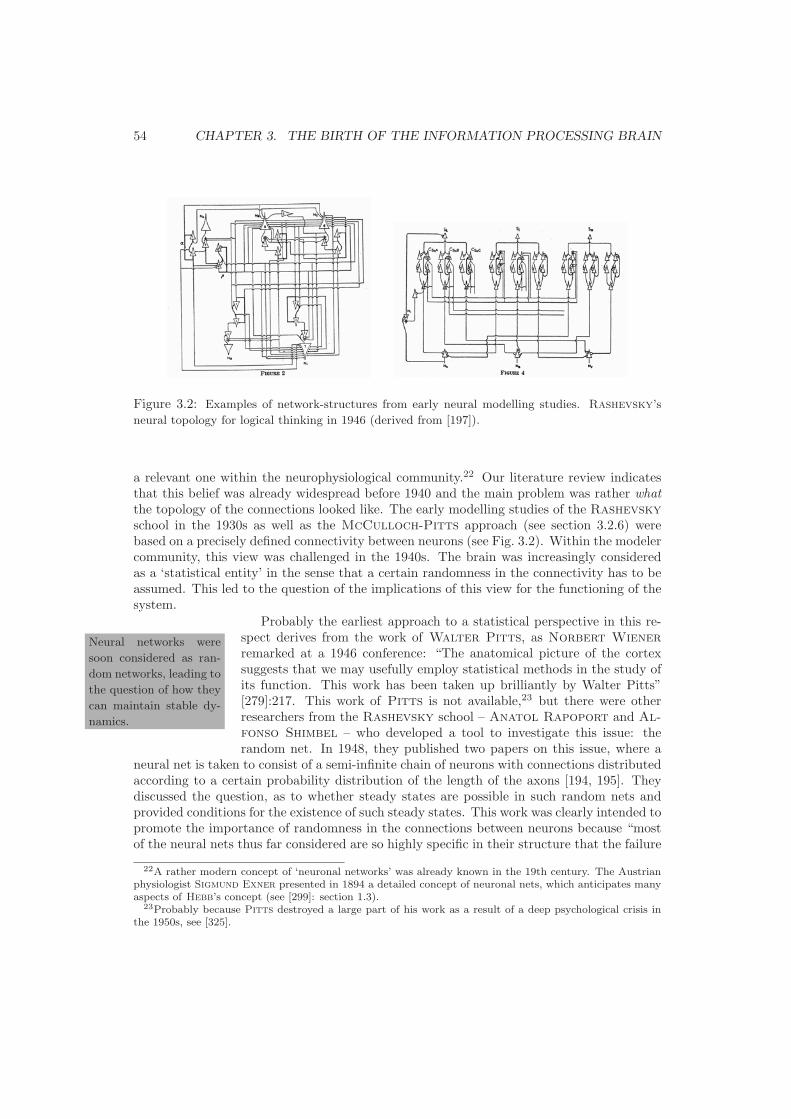
54 CHAPTER 3. THE BIRTH OF THE INFORMATION PROCESSING BRAIN
Figure 3.2: Examples of network-structures from early neural modelling studies. Rashevsky’s
neural topology for logical thinking in 1946 (derived from [197]).
a relevant one within the neurophysiological community.22 Our literature review indicatesthat this belief was already widespread before 1940 and the main problem was rather whatthe topology of the connections looked like. The early modelling studies of the Rashevsky
school in the 1930s as well as the McCulloch-Pitts approach (see section 3.2.6) werebased on a precisely defined connectivity between neurons (see Fig. 3.2). Within the modelercommunity, this view was challenged in the 1940s. The brain was increasingly consideredas a ‘statistical entity’ in the sense that a certain randomness in the connectivity has to beassumed. This led to the question of the implications of this view for the functioning of thesystem.
Neural networks were
soon considered as ran-
dom networks, leading to
the question of how they
can maintain stable dy-
namics.
Probably the earliest approach to a statistical perspective in this re-spect derives from the work of Walter Pitts, as Norbert Wiener
remarked at a 1946 conference: “The anatomical picture of the cortexsuggests that we may usefully employ statistical methods in the study ofits function. This work has been taken up brilliantly by Walter Pitts”[279]:217. This work of Pitts is not available,23 but there were otherresearchers from the Rashevsky school – Anatol Rapoport and Al-
fonso Shimbel – who developed a tool to investigate this issue: therandom net. In 1948, they published two papers on this issue, where a
neural net is taken to consist of a semi-infinite chain of neurons with connections distributedaccording to a certain probability distribution of the length of the axons [194, 195]. Theydiscussed the question, as to whether steady states are possible in such random nets andprovided conditions for the existence of such steady states. This work was clearly intended topromote the importance of randomness in the connections between neurons because “mostof the neural nets thus far considered are so highly specific in their structure that the failure
22A rather modern concept of ‘neuronal networks’ was already known in the 19th century. The Austrianphysiologist Sigmund Exner presented in 1894 a detailed concept of neuronal nets, which anticipates manyaspects of Hebb’s concept (see [299]: section 1.3).
23Probably because Pitts destroyed a large part of his work as a result of a deep psychological crisis inthe 1950s, see [325].

3.2. 1940-1970: DETAILED ANALYSIS 55
of even one neuron to function renders the entire mechanism useless” [232]:41. In 1950,Shimbel wrote that the “most serious shortcoming of the method of McCullloch-Pitts
lies in the fact that it assumes an extremely detailed knowledge of the neural pattern underconsideration” [231]:242. As an alternative approach, “the notion of probability in study-ing the structure and function of the nervous system” [231]:243 must be considered. Alsoat the famous Hixon symposium in 1948, this point was discussed. Lashely said: “Theanatomical variability [of the nervous system] is so great as to preclude, I believe, any theorywhich assumes regularity and precision of anatomical arrangements. Such facts lead me tobelieve that theories of neuron interaction must be couched, not in terms of the activity ofindividual cells but in terms of mass relations among the cells” [128]:70. The zoologist Paul
Weiss expressed a similar opinion: “The study of the developed nervous system, with whichthe anatomist, physiologist, and psychologist are usually working, suggests a high degree ofprecision in the arrangement of the constituent elements, but it must be realized that thisimpression is illusory. The organizational stability of a performance of the nervous systemis much greater than the precision of the underlying structural apparatus” [128]:72-73.
The requirement for randomness concerning neuronal connectivity was soon adopted bythe modeler community, although they had now to solve the problem of how the requirementfor a random assembly of elements can be linked with stable dynamics: Ross Ashby ana-lyzed this problem in 1950 using a purely mathematical model and came to the conclusionthat “randomly assembled dynamical systems have only a small chance of being stable. (...)So it is clear, for instance, that in a discussion of cerebral dynamics one may not postu-late a randomly assembled system unless one is prepared to accept the implied instability”[20]:481. Ashby, however, changed his opinion on this matter, as two years later he declaredin his monograph Design for a Brain randomness in connectivity to be a necessary propertyof neuronal systems: “Any system which shows adaption must (...) be assembled largely atrandom, so that its details are determined not individually but statistically” [19]:v.
In the 1950s, random connections in neural nets forming the cerebral cortex became anassumption for several important models: Karl Pribram mentioned in a review in 1960 inthis respect the models of Hebb, Licklider, MacKay, Milner, and Uttley [184]:26-27.A.M. Uttley emphasized the need for a statistical approach very clearly: “There is reasonto believe that many of the complexities of the cerebral cortex are due to an organization thatis fundamentally of a statistical nature” [233]. He used this approach to build a card-sortermachine, where the connections between the input elements and the indicators are randomlyassigned. His machine was able to classify punch-cards, which he took as an indication thatsimilar processes may be at work in the nervous system: “Assuming that connections areformed as a result of this chance proximity, it can be shown that a classification system willarise to some extent” [254]:482.
An influential contribution was provided by R.L. Beurle in 1956 [30]. He discussed theproblem of how activity in a randomly connected net of model neurons spreads, and whathappens if some property of the individual cell – like size, extent of the axon, dendritic struc-ture or threshold – changes with repeated use. Beurle’s work is based on the assumption,that the “apparently very large random factor in the distribution of neurons and the wayin which their dendrites and axon fibres spread amongst each other” is a marked featureof certain parts of the cortex [30]:56. He also sets his work in opposition to the automataapproach (see next section): “The comparisons that have been made in the past betweenthe properties of computing machines and living organisms are interesting when made in
56 CHAPTER 3. THE BIRTH OF THE INFORMATION PROCESSING BRAIN
relation to abstract fundamental concepts, but less productive when details are considered.This is because, in the detailed design of most large computing machines, components areconnected together exactly according to some specification, and have a precise function inrelation to all other components. This specific organization in a computer contrasts with theapparently very large random factor in the interconnexions between neurons in many partsof the cortex” [30]:83. At that time, there was not much statistical information availableabout the structure of the cortex, so, as Beurle notes, one might still have the opinionthat the random structure of the mass of cells he considered does not bear a very closerelationship to the actual physiological structure. The main point, however, is that simpleand ordered forms of activity-spread can be observed in such a network: plane, spherical andcircular waves and vortex effects. There was, however, also the problem that his networkof simple model neuron often tended either to become completely quiescent or completelyactive. This was interpreted that the mass has a sensitive threshold for stimulation andmay act as an on/off switch comparable to the shifting of attention in an organism. Byimplementing modifications of the elements, trial and error learning, conditioned responses,and the ability to regenerate internally a sequence of past events can be observed. Thus, aconnection between ordered structures of behavior resulting from a probabilistic microstruc-ture was established – or in the words of Beurle: “(...) some of the basic forms of behaviorof living organisms can be simulated by a mass of simple units without the necessity ofpostulating a large degree of specific organization of these units” [30]:83. This is a majorinsight that inspired later probabilistic approaches to the nervous system.
However, the problem of how a highly connected, but randomly connected aggregate ofneurons is able to maintain a state of intermediate activity was not satisfyingly solved. In1962, Ashby, von Foerster and Waker provided a more realistic analysis of this matter:again the network evolved in either a completely quiet or a completely active state [18]. Oneyear later, J.S. Griffith offered a solution in his study using the same model of Ashby
and colleagues. He showed that the desired stability could be achieved by allowing eithersome order in connectivity on a large scale or by introducing inhibitory connections [107].The assumption of random connections later also served as a guiding principle for neuralnetworks, as fo example Frank Rosenblatt pointed out [204]. This aspect, however, willnot be discussed by us.
3.2.5 The Active and Reliable Brain
The ‘noisy’ and ‘sponta-
neously active’ brain was
soon be considered as a
model for technology.
Many different empirical and theoretical investigations in the period from1940 to 1970 focussed on the activity of the whole brain or large parts ofit, for example the studies on learning by Donald Hebb, or the use of theEEG. We, however, will focus only one aspect: how the notion of a ‘spon-taneous active’ brain was consolidated in that period and to what extentthis led to the problem of how ‘reliable’ system behavior could result from‘unreliable’ components. The latter was discussed in the emerging theory
of automata and computer science and became an important aspect of the brain-computeranalogy. In the 1950s and 1960s, a line has been drawn between a period before the 1940s,when the brain was considered as ‘passive reflex machine’, and the time after the 1940s,when the brain had become an ‘active device’. In Delisle Burns’s monograph on Theuncertain nervous system that appeared 1968, this point of view is well-documented: “Un-

3.2. 1940-1970: DETAILED ANALYSIS 57
til some twenty years ago, attempts to explain function in the intact nervous system werenecessarily dependent upon the results of experiments employing relatively large stimulat-ing and recording electrodes. (...) As a result, the physiologist unwittingly left his readerswith an impression that central neurones only discharged when instructed to do so by aneurophysiologist – the system appeared to be an immense assembly of wholly predictablerelationships. The widespread, recent use of micro-electrodes has done much to alter thispicture. One is now forced to think of most, if not all, central neurones as continually active”[57]:162. We showed (see section 2.3.1) that such a sharp transition line cannot be drawn,as there were experimental findings and theoretical models in which ‘spontaneous activity’was playing a role, well before the 1940s. However, the ‘active brain’ became the dominantidea after 1940. An important promotor of this point of view is certainly Karl Spencer
Lashley. He expressed this opinion very clearly at his talk on The Problem of Serial Orderin Behavior at the Hixon symposium in 1948:
“Neurological theory has been dominated by the belief that the neurons ofthe central nervous system are in an inactive or resting state for the greater partof the time (...). Such a view is incompatible both with the widespread effects ofstimulation which can be demonstrated by changes in tonus and also with recentevidence from electrical recording of nervous activity. (...) It is probably not farfrom the truth to say that every nerve cell of the cerebral cortex is involved inthousands of different reactions. The cortex must be regarded as a great networkof reverberatory circuits, constantly active” [139]:131.
Lashley contrasted his concept with the more static model of McCulloch and Pitts
(see next section), where neurons are embedded in networks performing logical functions. Herather proposed that “the analysis must be extended to the properties of such nets, the wayin which they are broken up into reactive patterns in the spread of excitation, to give, forexample, directional propagation or its equivalent. I strongly suspect that many phenomenaof generalization, both sensory and conceptual, are products, not of simple switching, butof interaction of complex patterns of organization within such systems” [139]:134. Lashley
emphasized this point in the discussion following his talk: “I agree thoroughly with Dr.McCulloch that the transmission of excitation by the individual neuron is the basic prin-ciple of nervous organization. However, the nervous activity underlying any bit of behaviormust involve so many neurons that the action of any one cell can have little influence uponthe whole. I have come to feel that we must conceive the nervous activity in terms of theinterplay of impulses in a network of millions of active cells” [139]:145
In the 1950s, the ‘spontaneous activity’ of several neural (sensory) system was investi-gated, where the term ‘spontaneous’ is usually understood as denoting the “activity observedin the experimental situation in the absence of deliberate stimulation” [151]:377 (see also[136]:697). Donald Hebb made clear that the term ‘spontaneous’ would not involve anynon-mechanistic, metaphysical forces acting within the system: “Spontaneity of firing bycentral neural cells is not philosophic indeterminacy, as some writers have thought; the‘spontaneity’ means only that synaptic stimulation is not the sole cause of firing” [119].These studies in sensory systems have usually been put in the context of the ‘noise’ prob-lem. In that sense, spontaneous activity was one aspect of noise that disturbs informationtransmission (see section 3.2.2). S.W. Kuffler, however, presented an alternative view in
58 CHAPTER 3. THE BIRTH OF THE INFORMATION PROCESSING BRAIN
the sense that the representation of information is just the modulation of the spontaneousactivity [136]:699. This line of argumentation leads to the discussion on the functional rele-vance of noise (see section 3.2.2). In the review of Pribram of 1960 [184], the studies madein Burns’ laboratory in the late 1950s [59] were considered as the ones that consolidatedthe concept of ‘spontaneous activity’. In these studies, brain tissue was completely isolatedneurally from other nervous tissue. In that case, the neurons are indeed quiescent, but alsoeasily aroused to prolonged activity: “Hence, at ‘rest’, they [the neurons] may be conceivedto be just below the excitatory level for continuous self-excitation” [184]:2. In 1962, Burns,together with G.K. Smith published another study demonstrating that in the unstimulated(cat) brain, almost all neurons exhibit spontaneous activity [58]. Thus, spontaneous activitywas an accepted phenomenon in the 1960s.
For the theoretically oriented neuroscientists, these findings posed a problem: How canthe neural system function when the neurons themselves are unreliable in the sense thatthey show variable response and spontaneous activity. For logical nets of the McCulloch-Pitts-type, this was indeed a problem, although there were some attempts in the 1960s toassess the stability of these nets in noisy conditions [39]. The interesting point is, however,that spontaneous activity, as well as the problem of random connectivity discussed earlier,was soon put in a technological context. Griffith for example, who provided a solution ofthe stability-problem of random nets (see prior section), declared in 1963 that “such masses[of randomly connected cells] are potentially useful for the construction of artificial brain-like systems” [107]:308. The fascinating question for the emerging ‘bionics’ communityin the early 1960s was, as von Foerster mentioned: “What are the structures whichmake complex systems immune against errors of all kinds?” [257]:x. A main figure in thisdiscussion was John von Neumann, who attacked the problem of the Synthesis of reliableorganisms from unreliable components (the title of his 1956-paper [267]) in a sophisticatedway. As a major problem concerning the construction of such systems he identified “notso much that incorrect information will be obtained, but rather that irrelevant results willbe produced” [267]:62. Not the single error is relevant, but the fact that errors accumulatesuch that the long-run behavior of the system is unreliable. To solve this problem, heintroduced the ‘multiple line trick’ or ‘multiplexing’ – which later led to the theory ofredundancy in computer design [181] –, a ‘majority rule’, and a ‘restoring organ’.24 In thisway, the system operates along several parallel pathways and is able to compare after eachprocessing step the outcomes of the parallelly processed information and, using the resultof this comparison, to maintain the correct outcome. The system is organized in such amanner, “that a malfunction of the whole automaton cannot be caused by the malfunctionof a single component, or of a small number of components, but only by the malfunctioningof a large number of them” [267]:70. Von Neumann’s solution, however, could only dealwith unreliability expressed in the components, but not in their connectivity. In 1963, S.
Winograd and J.D. Cowan included the latter aspect and came to a similar conclusion toGriffith, whereas randomness in connectivity within certain modules should be combined
24In 1957, also Henry Quastler noted the importance of redundancy: “It is possible that there is amessage for engineers in the organization of biological computers. Traditionally, the engineer’s ideal is toeliminate redundancy and to perfect elementary reliability, and this is achieved during a more or less extendedperiod of collecting case histories and correcting specific shortcomings. As systems become very complicated,this method becomes less and less feasible” [190]:194. The solution is thus to combine redundancy with lowelementary reliability.
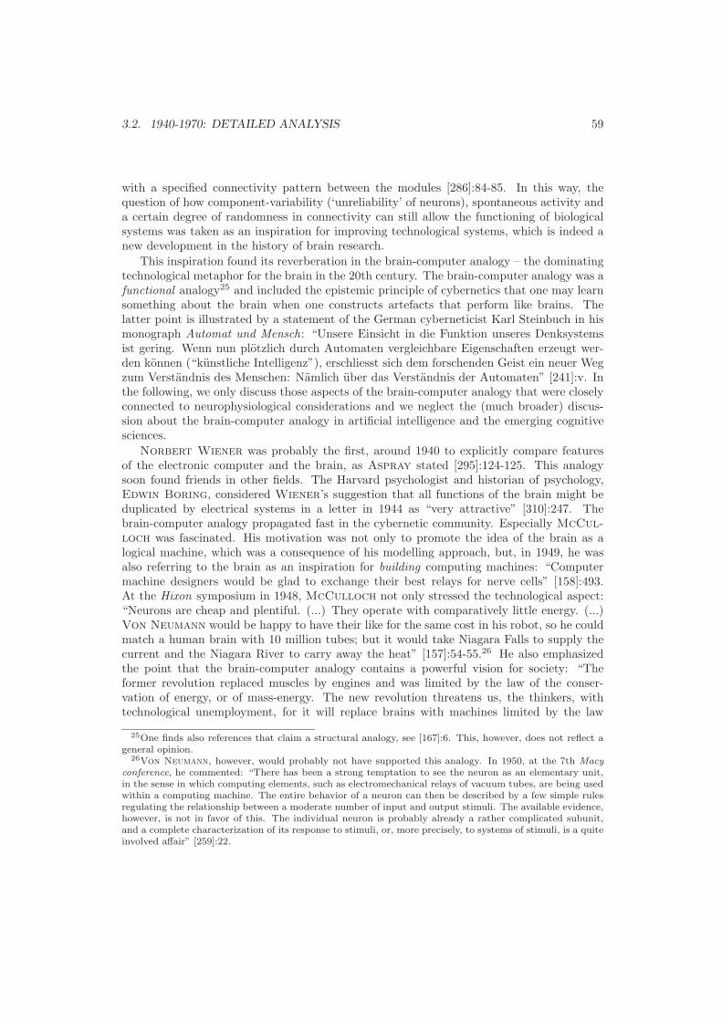
3.2. 1940-1970: DETAILED ANALYSIS 59
with a specified connectivity pattern between the modules [286]:84-85. In this way, thequestion of how component-variability (‘unreliability’ of neurons), spontaneous activity anda certain degree of randomness in connectivity can still allow the functioning of biologicalsystems was taken as an inspiration for improving technological systems, which is indeed anew development in the history of brain research.
This inspiration found its reverberation in the brain-computer analogy – the dominatingtechnological metaphor for the brain in the 20th century. The brain-computer analogy was afunctional analogy25 and included the epistemic principle of cybernetics that one may learnsomething about the brain when one constructs artefacts that perform like brains. Thelatter point is illustrated by a statement of the German cyberneticist Karl Steinbuch in hismonograph Automat und Mensch: “Unsere Einsicht in die Funktion unseres Denksystemsist gering. Wenn nun plotzlich durch Automaten vergleichbare Eigenschaften erzeugt wer-den konnen (“kunstliche Intelligenz”), erschliesst sich dem forschenden Geist ein neuer Wegzum Verstandnis des Menschen: Namlich uber das Verstandnis der Automaten” [241]:v. Inthe following, we only discuss those aspects of the brain-computer analogy that were closelyconnected to neurophysiological considerations and we neglect the (much broader) discus-sion about the brain-computer analogy in artificial intelligence and the emerging cognitivesciences.
Norbert Wiener was probably the first, around 1940 to explicitly compare featuresof the electronic computer and the brain, as Aspray stated [295]:124-125. This analogysoon found friends in other fields. The Harvard psychologist and historian of psychology,Edwin Boring, considered Wiener’s suggestion that all functions of the brain might beduplicated by electrical systems in a letter in 1944 as “very attractive” [310]:247. Thebrain-computer analogy propagated fast in the cybernetic community. Especially McCul-
loch was fascinated. His motivation was not only to promote the idea of the brain as alogical machine, which was a consequence of his modelling approach, but, in 1949, he wasalso referring to the brain as an inspiration for building computing machines: “Computermachine designers would be glad to exchange their best relays for nerve cells” [158]:493.At the Hixon symposium in 1948, McCulloch not only stressed the technological aspect:“Neurons are cheap and plentiful. (...) They operate with comparatively little energy. (...)Von Neumann would be happy to have their like for the same cost in his robot, so he couldmatch a human brain with 10 million tubes; but it would take Niagara Falls to supply thecurrent and the Niagara River to carry away the heat” [157]:54-55.26 He also emphasizedthe point that the brain-computer analogy contains a powerful vision for society: “Theformer revolution replaced muscles by engines and was limited by the law of the conser-vation of energy, or of mass-energy. The new revolution threatens us, the thinkers, withtechnological unemployment, for it will replace brains with machines limited by the law
25One finds also references that claim a structural analogy, see [167]:6. This, however, does not reflect ageneral opinion.
26Von Neumann, however, would probably not have supported this analogy. In 1950, at the 7th Macy
conference, he commented: “There has been a strong temptation to see the neuron as an elementary unit,in the sense in which computing elements, such as electromechanical relays of vacuum tubes, are being usedwithin a computing machine. The entire behavior of a neuron can then be described by a few simple rulesregulating the relationship between a moderate number of input and output stimuli. The available evidence,however, is not in favor of this. The individual neuron is probably already a rather complicated subunit,and a complete characterization of its response to stimuli, or, more precisely, to systems of stimuli, is a quiteinvolved affair” [259]:22.

60 CHAPTER 3. THE BIRTH OF THE INFORMATION PROCESSING BRAIN
that entropy never decreases” [157]:42. Donald MacKay, a companion of McCulloch
in this respect, saw also a link in direction of psychiatry. He hoped, that the knowledgegained by using this analogy may help to establish a “working link between the conceptsof psychiatry and those of physiology and anatomy.(...) The considerable effort going intothis theoretical model-making is justified chiefly by the hope that out of it may come a wayof describing the thinking process, sufficiently close to psychiatric realities to be useful indiagnosis, yet sufficiently operational and objective to allow the physiologist to make hismaximum contribution to the study and treatment of mental illness” [149]:266-267.
In the small community [295], in which the brain-computer analogy was developed, itslimitations had been realized. John von Neumann was probably the most careful in thisrespect. At the Hixon symposium, he stated: “It is very obvious that the brain differsfrom all artificial automata that we know; for instance, in the ability to reconstruct itself(as in the case of mechanical damage). It is always characterized by a very great flexibilityin the sense that animals with look reasonably alike and do the same thing, may do it byrather different cerebral mechanisms. Furthermore, though all humans belong to the samecategory and do the same things, outwardly, in some cases they are using different cerebralmechanisms for the same things, so there seems to be a flexibility of pathways” [128]:109.In his talk at the symposium, John von Neumann also took the analogy as an inspirationfor building a new type of automata. These systems should not be designed down to everydetail, but only “on some general principles which concern it, plus a machine which can putthese into effect, and will construct the ultimate automaton and do it in such a way that youyourself don’t know any more what the automaton will be” [128]:110. A (first) cumulationof this program was the publication of the anthology Automata Studies in 1956, whose listof contributors included the major protagonists in the field [225].27.
In the following years, the differences between brains and computers became the focusof research. Beside the points already mentioned above made by von Neumann, the in-trinsic activity of neural systems have also become a point that distinguishes them fromcomputers. Theodore Bullock noted in 1961: “Nervous systems are not like presentcomputers, even complex ones, but have oscillators and built-in stored patterns; they donot give outputs predictable by their inputs or externally controlled ‘instructions’ ” [54]:65.The issue of the brain-computer analogy was also disputed at a work session of the Neuro-sciences Research Program in 1964 about Mathematical concepts of central nervous systemfunction. H. Goldstine provided an overview of four main differences between brains andcomputers: 1) Computers function either analogically or digitally, but nervous systems ap-pear to function by a combination of the two methods. 2) Parts of the nervous system utilizefrequency-modulation coding rather than the binary coding of the computer. 3) The level ofmathematical precision of the nervous system is considerably less than that of a computer.4) Computers do not share with the brain its structural redundancy [236]:116 These obvi-ous differences as well as a critical attitude of many neurophysiologists toward modellingstudies led the cybernetics community to take this critique on board by using one of twostrategies, either weakening the analogy, or stressing that a ‘new’ concept of computationwill be necessary to understand biological computation. In his 1961 monograph with theprovocative title The Brain as a Computer, F.H. George acknowledged that “the brain is
27The contributors were: W.R. Ashby, J.T. Culberson, M.D. Davis, S.C. Cleene, K. de Leeuw, D.M.
MacKay, J. McCarthy, M.L. Minsky, E.F. Moore, C.E. Shannon, N. Shapiro, A.M. Uttley and J.
von Neumann.

3.2. 1940-1970: DETAILED ANALYSIS 61
clearly a vastly complicated system, and there is an obvious naivety – doubtless irritatingto a neurophysiologist – in such statements as, ‘just a switching device’, ‘the eyes are like atelevision scanning system’, ‘the brain is a complex digital (and analogue) computer’, andso one” [89]:310. He concluded that “we still have a very long way to go before we can fitall the empirical facts together, especially at the molecular level, to supply anything like theworking model we need” [89]:380. Ross Ashby was in favor of the second strategy. In his1966 review on the use of mathematical models and computer technology in neuroscience,he wrote: “What has been found by computer studies in the last ten years thus suggeststhat one central problem of the ‘higher’ functions in the brain is to discover its methods forprocessing information. The methods we know today tend to be inefficient to ‘astronomical’degree: the living brain may well know better” [17]:104. Some attempts to ‘copy’ the brainin this respect had already been undertaken at that time. One obvious example is the de-velopment of neural nets – whose history we cannot provide in this thesis. Another exampleis the founding of the Biological Computer Laboratory (BCL) by Heinz von Foerster atthe University of Illinois in January 1958.28 The BCL was in its initial phase an activepromoter of concepts like ‘self-organization’ and ‘bionics’ (this word was coined in 1958 ata conference organized by the BCL by John E. Steele) and turned later to the socialsciences. A complete history of how brain research inspired computer technology, however,remains to be written.
3.2.6 The Modelling Approach
Models were a permanent companion of brain research. The number of available models,however, increased considerably in the 1950s and 1960s. In 1964 Leon Harmon identifiedmore than 50 models that were created from 1940 to 1964 [115]:20. A literature review onthis subject in 1968 listed more than 500 articles devoted to neural modelling [144]:247. Wetherefore only briefly discuss the contributions of the Rashevsky school and the famousproposal made by McCulloch and Pitts in 1943. For a short contemporary review of1966 we refer to the publication of Harmon and Lewis [114]:519-530. Three causes arementioned when the usefulness of models is discussed [114]:516. First, models serve as akind of ‘summary’ of the current knowledge about the system under investigation. It isthus a prerequisite for a model that it is accurate both quantitatively and qualitatively withrespect to the phenomenon under investigation up to the degree of precision that has beenchosen by the investigator. Second, with validity tentatively established, one may attemptto discover new properties of the model, that might, for example, lead to new experiments.Third, the model may serve as a tool to test hypotheses about the system more rapidly andeconomically than direct physiological measurements permit.
The emergence of the computer as a research tool, however, supplemented this list. First,it changed the perspective towards the processes in the nervous system by putting an em-phasis on the information processing aspects of the nervous system. Harmon and Lewis
wrote in their 1966 review: “The advent of digital- and analog-computer technology, wellestablished by the mid-1950s, added new dimensions to the foundations on which neuro-physiological research is based. Nervous systems began to be considered more and moreexplicitly as processors of information, literally as biological computers” [114]:530. Second,
28Albert Muller has provided a historical overview of the BCL [329].
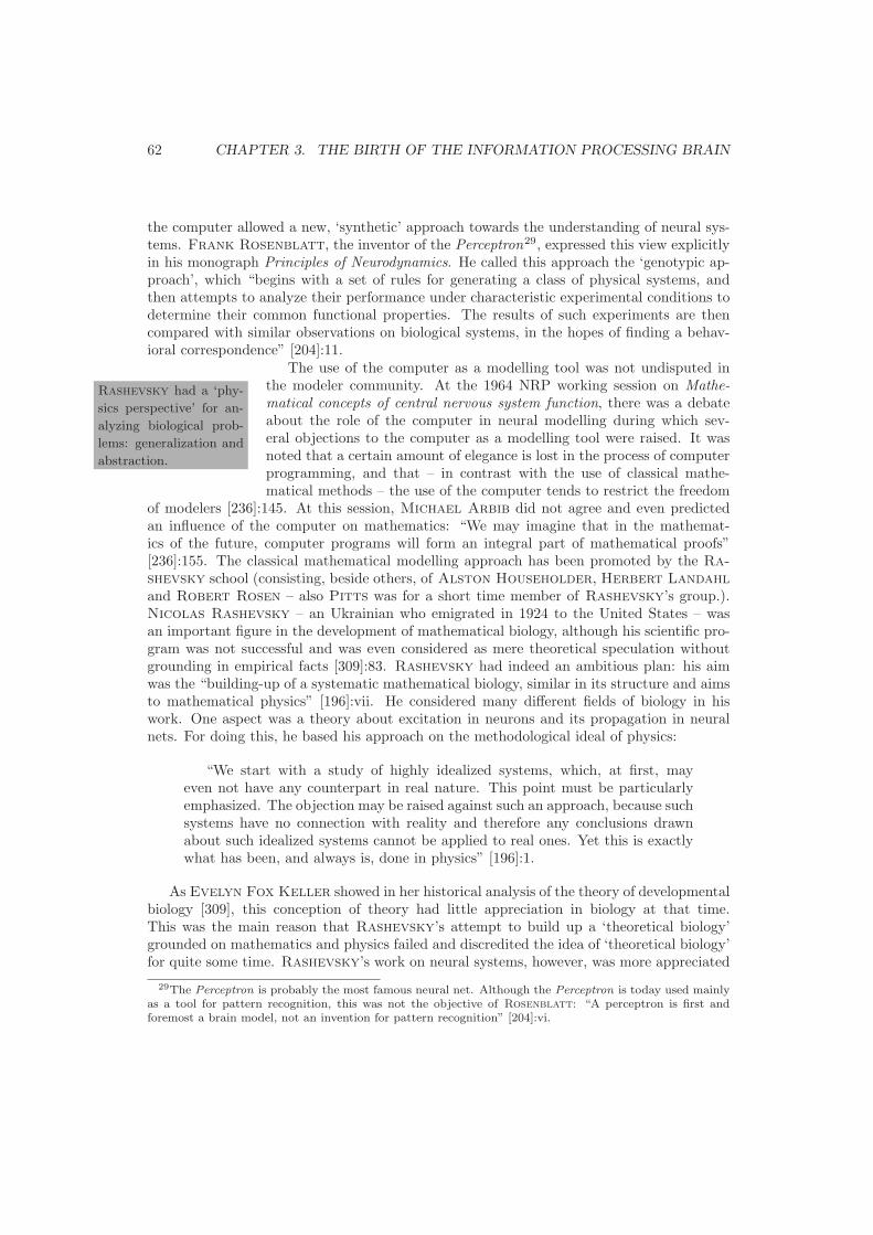
62 CHAPTER 3. THE BIRTH OF THE INFORMATION PROCESSING BRAIN
the computer allowed a new, ‘synthetic’ approach towards the understanding of neural sys-tems. Frank Rosenblatt, the inventor of the Perceptron29, expressed this view explicitlyin his monograph Principles of Neurodynamics. He called this approach the ‘genotypic ap-proach’, which “begins with a set of rules for generating a class of physical systems, andthen attempts to analyze their performance under characteristic experimental conditions todetermine their common functional properties. The results of such experiments are thencompared with similar observations on biological systems, in the hopes of finding a behav-ioral correspondence” [204]:11.
Rashevsky had a ‘phy-
sics perspective’ for an-
alyzing biological prob-
lems: generalization and
abstraction.
The use of the computer as a modelling tool was not undisputed inthe modeler community. At the 1964 NRP working session on Mathe-matical concepts of central nervous system function, there was a debateabout the role of the computer in neural modelling during which sev-eral objections to the computer as a modelling tool were raised. It wasnoted that a certain amount of elegance is lost in the process of computerprogramming, and that – in contrast with the use of classical mathe-matical methods – the use of the computer tends to restrict the freedom
of modelers [236]:145. At this session, Michael Arbib did not agree and even predictedan influence of the computer on mathematics: “We may imagine that in the mathemat-ics of the future, computer programs will form an integral part of mathematical proofs”[236]:155. The classical mathematical modelling approach has been promoted by the Ra-
shevsky school (consisting, beside others, of Alston Householder, Herbert Landahl
and Robert Rosen – also Pitts was for a short time member of Rashevsky’s group.).Nicolas Rashevsky – an Ukrainian who emigrated in 1924 to the United States – wasan important figure in the development of mathematical biology, although his scientific pro-gram was not successful and was even considered as mere theoretical speculation withoutgrounding in empirical facts [309]:83. Rashevsky had indeed an ambitious plan: his aimwas the “building-up of a systematic mathematical biology, similar in its structure and aimsto mathematical physics” [196]:vii. He considered many different fields of biology in hiswork. One aspect was a theory about excitation in neurons and its propagation in neuralnets. For doing this, he based his approach on the methodological ideal of physics:
“We start with a study of highly idealized systems, which, at first, mayeven not have any counterpart in real nature. This point must be particularlyemphasized. The objection may be raised against such an approach, because suchsystems have no connection with reality and therefore any conclusions drawnabout such idealized systems cannot be applied to real ones. Yet this is exactlywhat has been, and always is, done in physics” [196]:1.
As Evelyn Fox Keller showed in her historical analysis of the theory of developmentalbiology [309], this conception of theory had little appreciation in biology at that time.This was the main reason that Rashevsky’s attempt to build up a ‘theoretical biology’grounded on mathematics and physics failed and discredited the idea of ‘theoretical biology’for quite some time. Rashevsky’s work on neural systems, however, was more appreciated
29The Perceptron is probably the most famous neural net. Although the Perceptron is today used mainlyas a tool for pattern recognition, this was not the objective of Rosenblatt: “A perceptron is first andforemost a brain model, not an invention for pattern recognition” [204]:vi.
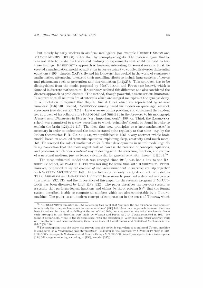
3.2. 1940-1970: DETAILED ANALYSIS 63
– but mostly by early workers in artificial intelligence (for example Herbert Simon andMarvin Minsky [309]:88) rather than by neurophysiologists. The reason is again that hewas not able to relate his theoretical findings to experiments that could be used to testthese findings. Rashevsky’s approach is, however, interesting for several reasons. First, hecreated a mathematical model of excitation in nerves using two coupled first-order differentialequations ([196]: chapter XXIV). He and his followers thus worked in the world of continuousmathematics, attempting to extend their modelling efforts to include large systems of nervesand phenomena such as perception and discrimination [144]:253. This approach has to bedistinguished from the model proposed by McCulloch and Pitts (see below), which isfounded in discrete mathematics. Rashevsky realized this difference and also considered thediscrete approach as problematic: “The method, though powerful, has one serious limitation:It requires that all neurons fire at intervals which are integral multiples of the synapse delay.In our notation it requires that they all fire at times which are represented by naturalnumbers” [196]:540. Second, Rashevsky usually based his models on quite rigid networkstructures (see also section 3.2.4). He was aware of this problem, and considered the randomnet approach of his collaborators Rapoport and Shimbel in the foreword to his monographMathematical Biophysics in 1948 as “very important work” [196]:xx. Third, the Rashevsky
school was committed to a view according to which ‘principles’ should be found in order toexplain the brain [124]:114-115. The idea, that ‘new principles’ or a ‘new mathematics’ isnecessary in order to understand the brain is stated quite regularly at that time – e.g. by theItalian theoretician E.R. Caianiello, who published in 1961 a very abstract ‘whole brainmodel’ based on so-called ‘neuronic equations’ explaining sleep, creativity (and much more)[62]. He stressed the role of mathematics for further developments in neural modelling: “Itis my conviction that the most urgent task at hand is the creation of concepts, equations,and problems, which offer a natural way of dealing with the structure, function, and controlof a neuronal medium, just as tensor calculus did for general relativity theory” [61]:101.30
The most influential model that was emerged since 1940, also has a link to the Ra-
shevsky school, as Walter Pitts was working for some time with Rashevsky. Pitts,however, published A logical calculus of the ideas immanent in nervous activity togetherwith Warren McCulloch [159] . In the following, we only briefly describe this model, asTara Abraham and Gualtiero Piccinini have recently provided a detailed analysis ofthis matter [292, 335] and the importance of this paper for the research program of McCul-
loch has been discussed by Lily Kay [322]. The paper describes the nervous system asa system that performs logical functions and claims (without proving it)31 that the formalsystem described is able to compute all numbers which are also computable by a Turing
machine. The paper uses a modern concept of computation in the sense of Turing, which
30Claude Shannon remarked in 1964 concerning this point that “perhaps the call for a ‘new mathematics’
reflects only that the problem is new to mathematicians” [236]:142. As a ‘new’ approach, however, that hasbeen introduced into neural modelling at the end of the 1960s, one may mention statistical mechanics. Someearly attempts in this direction were made by Wiener and Pitts, as J.D. Cowan remarked in 1967. Hefound it remarkable, “that in the 20 years since, with the exception of Wiener’s own rather abstract workon Hamiltonians and neuromechanics, there is no trace of Hamiltonians and Statistical Mechanics in thefield” [68]:186.
31The assumption that the paper had proven that the model is equivalent to a universal Turing machineis considered as a “widespread misinterpretation” [153]:xviii in the foreword by Seymour Papert to Mc-
Culloch’s monograph Embodiments of Mind, although McCulloch himself propagated this misconception[154]:368 (page numbering according to [153], see also [335]).

64 CHAPTER 3. THE BIRTH OF THE INFORMATION PROCESSING BRAIN
led McCulloch to the conclusion (stated in 1949) that “the brain is a logical machine”[158]:492. Furthermore, the simplifying assumptions (the all-or-none ‘law’ and the discretiza-tion of time) in the paper supported an information perspective towards the neural system inthe sense that spike trains can be considered as binary strings. The paper was accompaniedby a short extension, where Herbert Landahl, together with McCulloch and Pitts,introduced a statistical viewpoint in the sense that the logical relations among the actionsof neurons in a net have been converted into statistical relations among the frequencies oftheir impulses ([137] see also [124]:Part 3). The neurophysiology community largely ignoredthe paper, and even logicians had their doubts about the quality of the contribution.32 Onthe other hand, the paper had a tremendous theoretical influence among neural modelers aswell as computer scientists (see section 4.3).33 The automata approach towards modellingneuronal systems is considered as a direct result of the work of McCulloch and Pitts
[142]: vii, and even John von Neumann utilized the McCulloch-Pitts notation for thelogical design of the EDVAC computer (according to Goldstine [236]:117).34 The modelitself, however, was soon considered as an inadequate description of neuronal processes.
32Frederic Fitch wrote in his review on the paper: “Symbolic logic is used freely, and indeed rather
carelessly. The notation is unnecessary complicated, and the number of misprints is so great that the reviewerwas unable to decipher several crucial parts of the paper. (...) In any case there is no rigorous constructionof a ‘logical calculus’ ” [83]:49.
33Consider also the introduction to the re-issued paper of McCulloch-Pitts [294]:15-17.34
Goldstine’s comment is not quite correct, as von Neumann did not use the notation in the sameway as McCulloch and Pitts. In his famous First Draft of a Report on the EDVAC of 1945 [269], hemade a close neuron analogy in which he presented the neuron as a purely digital device, in contrast to hislater statements on the neuron at the Macy conferences. His First Draft is considered to be a foundingpaper on the modern digital computer and it is thus of considerable interest that the biological inspirationwas outlined rather extensively in this paper. The first EDVAC, however, was not build according to von
Neumann’s report, but by the Moore school design group. For a history of the EDVAC consider [314, 344].

Chapter 4
1940 – 1970: The Dynamics ofResearch
This chapter complements the historical analysis with bibliometric and sciento-
metric investigations. We we analyze the increase of the number of publications
and journals since the Second World War. We focus on major conferences and
investigate, to what extent they can be grouped in thematic clusters, which serve
for identifying protagonists that distributed ideas on neural coding and informa-
tion processing in different scientific communities. Based on a citation analysis,
the influence of selected protagonists will be further investigated. We conclude this
chapter by a summary of the historical analysis.
4.1 Journals and Publications
Journals serve as an important communication tool within scientific communities. Newtopics are accompanied by the founding of new journals or by an increase in the number ofarticles on the new topic. We investigate this matter for the time period since the SecondWorld War (the onsets of the databases used are 1945 and 1965) up to the present time.
Methods: We investigate the number of journals and publications using the Med-Line and the ISI Web of Knowledge databases.1 Both databases are hosted in theUnited States and introduce a well-known bias towards mainstream and anglophonejournals (latter will become important in the citation analysis). Referencing and pos-sible search strategies are not equivalent in both databases. To estimate the number ofneuroscience papers (‘neuro-papers’) dealing explicitly with neurons or neural systems
1MedLine is a public database hosted by the National Institutes of Health of the United States.Access via http://www.ncbi.nlm.nih.gov/entrez/query.fcgi. The database covers papers associatedwith biomedical research. The ISI Web of Knowledge is a integrated Web-based platform contain-ing the Science Citation Index Expanded, the Social Sciences Citation Index and the Arts & Human-ities Citation Index and is hosted by The Thomson Corporation. Access (subscription necessary) viahttp://go5.isiknowledge.com/portal.cgi/
65

66 CHAPTER 4. 1940 – 1970: THE DYNAMICS OF RESEARCH
in either database, we used the following search strategies: In the ISI Web of Knowledgedatabase, the ‘general search’ interface was used and we looked for papers that con-tained the truncated search term ‘neur∗’ in their title for periods of fife years, beginningin 1945 (onset of the database). The constraint ‘Title only’ was necessary, as papers upto 1991 are only accessible via title search, whereas papers after 1991 are accessible byfull-text-search (abstracts). In MedLine (onset of the database: 1965), the search in-volves titles and abstracts (if available) and truncation search is not possible. We usedthe boolean search expression ‘neuron OR neural’. The number of ‘coding’ and ‘infor-mation processing’ papers was only estimated for MedLine, as words indicating suchpapers tend more to show up in abstracts than in titles. We used the following booleansearch expressions: ‘(neuron OR neural) AND (code OR coding)’ for neural codingpapers, and ‘(neuron OR neural) AND (information AND processing)’ for neural infor-mation processing papers. To compare the results for the period 1991-2004, a similaranalysis has been performed using the ISI Web of Knowlede database. They confirmedthe results obtained by the MedLine analysis (results not shown). We estimated thenumber of neuroscientists by the members of the Society of Neuroscience (SfN)2 – theoldest and largest institution in neuroscience, founded in 1968 under the leadership ofthe psychologist Neil Miller, the biochemist (and later behavioral scientist) Ralph
Gerard and the neurophysiologist Vernon Mountcastle [305]:347.
We estimated the growth of the number of ‘neuroscience journals’ using the ISI Webof Knowledge database and by including all journals classified as ‘neuroscience’ journalsthat hat an impact factor of at least 2 in the Journal Citation Report of 2003.3 We com-plemented this list with journals known to be important for neuroscience or theoreticalneuroscience from the categories ‘behavior’, ‘biophysics’, ‘computer systems: artificialintelligence’, ‘computer systems: cybernetics’, ‘computer systems: interdisciplinary ap-plications’, ‘multidisciplinary sciences’ and ‘physiology’. For ‘theoretical neuroscience’journals, the impact-factor criterium has not been applied. The latter journals are(in brackets: impact factor, year of founding, journal country; ordered according totime of funding): Bulletin of Mathematical Biophysics (1.468, 1938, USA), since 1972:Bulletin of Mathematical Biology ; Biophysical Journal (4.463, 1960, USA); Kybernetik(1.933, 1961, Germany), since 1975: Biological Cybernetics; Journal of Theoretical Bi-ology (1.550, 1961, USA); BioSystems (0.971, 1967, England); IEEE Transactions onSystems, Man and Cybernetics (1.029 (B), 1971, USA): separated later in three partsA,B,C; Neural Networks (1.774, 1988, England); Neural Computation (2.747, 1989,USA); Neurocomputing (0.592, 1989, Netherlands); Network: Computation on Neu-
2Access via www.sfn.org3The following journals listed in our journal count (see below) were present or were founded during 1940-
1970 (in brackets: year of founding, today’s journal country): Proceedings of the Royal Society of London(1841, England), Nature (1869, England), Proceedings of the National Academy of Sciences USA (1877,USA), Brain (1878, England), Journal of Physiology – London (1878, England), Behavioral Neuroscience(1887, USA), Clinical Neurophysiology (1897, Ireland), Journal of Comparative Neurology (1891, USA),Science (1895, USA), American Journal of Physiology (1898, USA), Journal of General Physiology (1918,USA), Physiological Review (1921, USA), Journal of Experimental Biology (1927, England), Journal ofNeurophysiology (1938, USA), Annual Review of Physiology (1939, USA), Journal of Neuropathology andExperimental Neurology (1942, USA), Journal of Neurochemistry (1956, England), Experimental Neurology(1959, USA), Biophysical Journal (1960, USA), Acta Neuropathologica (1961, Germany), Kybernetik (1961,Germany), Journal of Theoretical Biology (1961, USA), Neuropharmacology (1962, England), Neuropsy-chologia (1963, England), Journal of Neurological Sciences (1964, Netherlands), Psychophysiology (1964,USA), Biological Psychiatry (1965, USA), Neuroendocrinology (1965, Switzerland), Cortex (1965, Italy), Ex-perimental Brain Research (1966, Germany), BioSystems (1967, England), Frontiers in Neuroendocrinology(1969, USA), Psychopharmacology (1969, Germany) and Journal of Neurobiology (1969, USA).

4.1. JOURNALS AND PUBLICATIONS 67
1970 -1974
1975 -1979
1980 -1984
1985 -1989
1990 -1994
1994-1999
2000 -2004
a)
b)
1965 -1969
1
2
3
4
Ratio[%] Neuro vs. all
Code vs. neuro
Processing vs. neuro
20'000
40'000
60'000
80'000
100'000
120'000
45-49
50-54
5559
60-64
65-69
70-74
75-79
80-84
85-89
90-94
95-99
00-04
SfN members
Neuro-papers in ISI
Neuro-papers in MedLine
# papers / members
Figure 4.1: The neuroscience boom since the Second World War: a) Increase of the number of
‘neuro-papers’ contained in the MedLine and the ISI Web of Knowledge databases. b) Relative
increase of the number of ‘neuro-papers’ and of ‘neural coding’ and ‘neural information processing’
papers in MedLine (see text).
ral Systems (2.208, 1990, England); IEEE Transactions on Neural Networks (1.666,1990, USA); Neural Computation Applications (0.449, 1992, USA); Journal of Com-putational Neuroscience (2.776, 1994, USA); Neural Processing Letters (0.631, 1994,Belgium); Neuroinformatics (-, 2003, USA). In this way, a total of 130 ‘important jour-nals’ has been obtained. For each journal, its funding year (= the year of publishing ofthe first issue) and its present home country (publisher) have been evaluated.
The bibliometric analysis confirms the expected increase of publication activity in neuro-science: both databases show a similar increment in absolute number, which is furthermorecomparable to the growth of the number of scientists (Fig. 4.1.a). The ratio of all ‘neuro-papers’ compared to all papers indexed in MedLine demonstrate an increasing interest inneuroscience within biological and medical research in general. Finally, the ratio of all ‘neu-ral coding papers’ and ‘neural information processing papers’ compared to all ‘neuro-papers’point out an increasing interest in explicitly addressing neural coding or neural informationprocessing as a topic of research (Fig. 4.1.b). Remind, that the absolute numbers obtainedby the analysis should be taken with a pinch of salt, as the search strategies used are notexhaustive. However, this first approximation on the dynamics of research in neuroscienceindicates that analyzing the brain by explicitly focussing on its information processing ca-
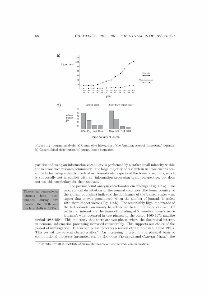
68 CHAPTER 4. 1940 – 1970: THE DYNAMICS OF RESEARCH
USA Eng Ned Rest USA Eng Ned Rest
10
2030
4050
60
relativefraction[%]
Journal count Scaled with impact factor
Home country of journal
45-49
50-54
5559
60-64
65-69
70-74
75-79
80-84
85-89
90-94
95-99
00-04
140
120
100
80
60
40
20
# journals
All journals
Theoretical journals
a)
b)
year
Figure 4.2: Journal analysis: a) Cumulative histogram of the founding years of ‘important’ journals.
b) Geographical distribution of journal home countries.
pacities and using an information vocabulary is performed by a rather small minority withinthe neuroscience research community. The large majority of research in neuroscience is pre-sumably focussing either biomedical or bio-molecular aspects of the brain or neurons, whichis supposedly not in conflict with an ‘information processing brain’ perspective, but doesnot use this vocabulary for their analysis.
Theoretical neuroscience
journals have been
founded during two
phases: the 1960s and
the late 1980s to 1990s.
The journal count analysis corroborates our findings (Fig. 4.2.a). Thegeographical distribution of the journal countries (the home country ofthe journal publisher) indicates the dominance of the United States – anaspect that is even pronounced, when the number of journals is scaledwith their impact factor (Fig. 4.2.b). The remarkably high importance ofthe Netherlands can mainly be attributed to the publisher Elsevier. Ofparticular interest are the times of founding of ‘theoretical neurosciencejournals’, what occurred in two phases: in the period 1960-1971 and the
period 1988-1994. This indicates, that there are two phases where the theoretical interestin neuronal information processing increased considerably. This supports our choice of theperiod of investigation. The second phase indicates a revival of the topic in the mid 1980s.This revival has several characteristics:4 An increasing interest in the physical basis ofcomputational processes (promoted e.g. by Richard Feynman and Carver Mead), the
4Rodney Douglas, Institute of Neuroinformatics, Zurich: personal communication.

4.2. CONFERENCES 69
Conference name, source Date Place # Part. Abbr.1. Macy conference, [333]:383 08./09. March 1946 New York 21 M1+
2. Macy conference, ASC 17./18. October 1946 New York 25 M2+
3. Macy conference, ASC 13./14. March 1947 New York 26 M3+
4. Macy conference, ASC 23./24. October 1947 New York 23 M4+
5. Macy conference, ASC Spring 1948 New York 28 M5+
6. Macy conference, [258] 24./25. March 1949 New York 23 M67. Macy conference, [259] 23./24. March 1950 New York 24 M78. Macy conference, [260] 15./16. March 1951 New York 23 M89. Macy conference, [262] 20./21. March 1952 New York 27 M910. Macy conference, [263] 22.-24. April 1953 Princeton, NJ 28 M10
Table 4.1: Conferences of the Macy-cluster. Abbreviation: ASC: American Society for Cybernetics.
The exact date of the 5th Macy conference could not be evaluated. Abbreviation marked with +
indicate members of a stable sub-cluster (see Fig. 4.3).
revival of the neural network approach after the introduction of the Hopfield-network,and the Carmel symposium Computational Neuroscience in 1987. In 1988, Terrence
Sejnowski, Christoph Koch and Patricia Churchland reviewed the research programof the new field ‘computational neuroscience’ [665] in an article in Science. In the 1990s,several new institutes in computational neuroscience (or neuroinformatics, the term used inEurope) have been founded. This second phase is not subject of our historical analysis.
4.2 Conferences
Conferences are important scientific marked places, where new ideas and concepts are pre-sented. The analysis of our historical sources led to the identification of several conferences,where neural coding and related issues had been discussed. In this section, we group themaccording to similarities such that ‘clusters’ of conferences represent scientific communities.This serves as a basis to identify persons (next section), that are present in several clustersand serve as ‘ambassadors’ of scientific ideas. We investigated the major conferences in thefields cybernetics (with focus on the Macy conferences), information theory in relation tobiology and neuroscience in relation to the Neurosciences Research Program as well as con-ferences that focus neural modelling and theoretical aspects. We did, however, not intendto analyze all conferences in the fields mentioned that happened between 1940 and 1970,as this would be far too ambitious. We have chosen the following conferences: For cyber-netics, we mainly focussed on the Macy conferences5 (10 conferences). For neuroscience,
5Sources: The re-issued Macy Proceedings [332, 333] and the website of the American Society for Cy-bernetics (ASC): http://www.asc-cybernetics.org/foundations/history/MacySummary.htm#Part1. Theparticipant lists given by the ASC and listed in the original publication did not always match. We used theoriginal numbers whenever possible provided by [332]. For the years 1946 (October), 1947 and 1948 we re-ferred to the ASC numbers. The representative of the Joshia Macy Jr. Foundation, Frank Fremont-Smith,was included in the count. The Macy meeting 1942 on “cerebral inhibition” with 20 participants[261]:xix –among them members of the later core group of the Macy conferences like Gregory Bateson, Lawrence
Frank, Frank Fremont-Smith, Lawrence Kubie, Warren McCulloch, Margaret Mead and Arthur
Rosenblueth – was not considered in the analysis. The Joshia Macy Jr. Foundation Conference Programalso included a series of five conferences on the ‘Nerve Impulse’ from 1950 to 1954 [166]. Based on our (notenclosing) analysis, these conferences focussed on physiological aspects like action potential generation and

70 CHAPTER 4. 1940 – 1970: THE DYNAMICS OF RESEARCH
Conference name, source Date Place # Part. Abbr.NRS summaries 1 (9), [221] 1963-64 Cambridge, MA 108 N1NRS summaries 2 (6), [220] 1965-66 Cambridge, MA 102 N21. ISP, [187] July 1966 Boulder, CO 64* N3NRS summaries 3 (6), [219] 1967-68 Cambridge, MA 97 N4NRS summaries 4 (5), [218] 1966-1968 Cambridge, MA 108 N5NRS summaries 5 (5), [216] 1967-1969 Cambridge, MA 114 N62. ISP, [217] 21.07. - 08.08. 1969 Boulder, CO 92* N7NRS summaries 6 (5), [215] 1968-70 Cambridge, MA 103 N8NRS summaries 7 (4), [214] 1970-71 Cambridge, MA 85 N9
Table 4.2: Work sessions and ISP of the NRP-cluster. In brackets: number of work sessions.
Abbreviations: NRS: Neurosciences Research Symposium. ISP: Intensive Study Program. Numbers
of participants marked with * indicate the number of contributing authors and not of participants.
we focussed on the activity of the Neurosciences Research Program in the 1960s and early1970s, which are published in a series of proceedings and monographs (45 work sessions and3 Intensive Study Programs).6 Figure 4.3.a provides an overview of the distribution of theconferences over the time of investigation, indicating, that the majority of the conferences(especially the NRP work session) were located in the 1960s. As we were not interested in adetailed analysis of clustering of topics within the NRP sessions, the 45 NRP work sessionshave been aggregated into eight groups according to the participant lists of the NeuroscienceResearch Symposium Summaries. Finally, all conferences, that were found during our searchfor historical sources, were considered (17 conferences). This lead to a total of 38 ‘confer-ences’ that were analyzed as described in the methods section below. In a contemporaryoverview in 1961 by the German cybernetics Karl Steinbuch [241]:136, more potentiallyinteresting conferences were listed: The first (1949) and the second (1952) London sympo-sium on information theory7, the second and third (1958,1961) Congres International deCybernetique in Namur (Belgium), and several conferences about the emerging computerscience that have taken place since the mid 1950s, for example the World Conferences ofthe International Federation for Information Processing (IFIP, in 1959, 1962, 1965, 1968for the period of interest), the National Conventions of the Institutes of Radio Engineers(together with the American Institute of Electrical Engineers the precursor of the Instituteof Electrical and Electronics Engineers) and the National Conferences of the Association ofComputing Machinery.8.
Methods: To obtain the conference clusters, we use the sequential superparamagneticclustering paradigm (for details, see section 7.5). Two different types of ‘distances’
not on coding issues.6Source: [212, 213, 214, 215, 216, 217, 218, 219, 220, 187, 221]. The events were called “work session’,
workshop’ or ‘symposium’ – we use ‘work session’ as general term. The work sessions usually took place atthe MIT [338]. For our analysis, we only considered those work sessions that were published in the sevenvolumes of the Neuroscience Research Symposium Summaries. The fourth Intensive Study Program of 1977has been excluded from the analysis.
7These conferences focussed on either mathematical and philosophical aspects or telecommunicationaspects [66]:v and did not discuss applications on biological questions.
8We took a sample (IFIP-proceedings: http://www.informatik.uni-trier.de/ ley/db/conf/ifip/ and[129]) to check whether neuro-related aspects were discussed to a considerable amount at those conferences.The result indicated, that applications on biological systems and problems played probably only a veryremote role within these conferences at that time.

4.2. CONFERENCES 71
between conferences are applied: The first distance measure, the participant distance,is given as the size of the intersection of the participant sets of two conferences. Inthat way, two conferences are ‘close’ if the same people participate in both conferences.To calculate the participant distance, we created a database containing all names ofresearchers that were either listed as participants or – if a participant list was notavailable – listed as contributors to the proceedings. The name data base contains1481 names, whereas we have checked in three independent runs to verify name iden-tities. For the NRP work sessions, we created aggregated lists according to the 8volumes of the Neuroscience Research Symposium Summaries, covering 4 to 9 worksessions. The pairwise comparison of all conferences leads to the sizes of intersectionsets. The obtained numbers are normalized by the largest intersection set, and then 1 issubtracted. The absolute value of the result is taken as the distance between two con-ferences. Thus, a distance 0 indicates that exactly the same participants were presentin both conferences, and a distance 1 indicates, that no person was in both conferences.The resulting distance matrix is used as input for the clustering algorithm.
The second distance measure, the topic distance, follows the idea, that two confer-ences are close if the relative number of contributions that have been assigned to certaintopics are similar. For each conference, a six-dimensional ‘topic vector’ is constructedby counting the number of contributions that fall into the following classes:
• Theoretic: Contributions of the fields mathematics, physics, statistics and infor-mation theory.
• Molecular Level : Contributions that deal with aspects of the molecular biologyof cells/neurons like genetic studies, protein studies, and membrane studies.
• Neuron Level : Contributions that deal with very small neuronal networks, singleneurons or parts of neurons, e.g. electrophysiological input-output-studies, spiketrain analysis, work on synapses, coding properties of single neurons or smallneuronal networks, influence of chemicals on single cells, as well as biomorphicmodelling on the single neuron level.
• Neuronal System: Contributions that deal with brains and neuronal networks ona ‘system-level’ and is based on, or is in close connection to, experimental work inbiological systems , e.g. sensory and motor systems, developmental aspects, EEGstudies, neuroanatomy, as well as biomorphic modelling on a systems level.
• Behavioral : Contributions dealing with social systems, language, learning and be-havior without linking this analysis with experimental work in neuronal systems.
• Cybernetic: Contributions of the fields automata theory, ‘pure’ (non-biomorphic)modelling, and theories of control and self-organization
Each ‘topic vector’ is normalized by the total number of the Contributions. Thedistance between two conferences is obtained by calculating the dot product betweentwo vectors, subtracting 1 from the result and taking the absolute value. In this way,the distance 1 indicates that the topic vectors are orthogonal (i.e. the conferences dealtwith completely different topics) and a distance 0 indicates, that in both conferencesbasically the same topics were discussed to the same degree. Again, the resultingdistance matrix is used as input for the clustering algorithm. As the topic distancecontains more ambiguity (in assigning contributions to classes) than the participantdistance, latter will be used for identifying scientific communities (clusters) and formeris used for validating the results.

72 CHAPTER 4. 1940 – 1970: THE DYNAMICS OF RESEARCH
Conference name, source Date Place # Part. Abbr.The Hixon Symposium, [128] 20.-25. Sept. 1948 Pasadena, CA 19 T1Information Theory in Biology, [191] Summer 1952 Urbana, IL 15* T23. Symposium on Inf. Theory, [66] 12.-16. Sept. 1955 London, UK 50* T3+
1er congr. int. de cybernetique, [186] 26.-29. June 1956 Namur, Belgium 79* T4+
Information Theory in Biology, [287] 29.-31. Oct. 1956 Gatlinburg, TN 32* T5Mechan. of Thought-Processes, [169] 24.-27. Nov. 1958 Teddington, UK 211 T6+
Self-Organizing Systems, [289] 05.-06. May 1959 Chicago, IL 19* T7+
4th Symposium on Inf. Theory, [67] 29.08. - 02.09. 1960 London, UK 53* T8+
Principles of Self-Organization, [257] 08./09. June 1961 Urbana, IL 39 T9+
Inf. Storage and Neural Control, [81] 1962 Houston, TX 16 T10Cybernetic Problems in Bionics, [170] 03.-05. May 1966 Dayton, OH 69* T11+
School on Neural Networks, [60] June 1967 Ravello, Italy 22* T12+
Inf. Proc. in the Nervous Sys., [142] 21.-24. Oct. 1968 Buffalo, NY 67 T13+
Table 4.3: Theory-Cluster. Numbers of participants marked with * indicate the number of con-
tributing authors and not of participants. Abbreviation marked with + indicate members of a stable
sub-cluster (see Fig. 4.3).
The cluster analysis led to the following result: Using the participant distance, fourclusters are identified: The most stable cluster is – as expected – the Macy cluster (Table4.1). The conferences of this cluster are close by construction, as the Macy conferences wereorganized around a large core-group of participants. The Macy cluster is subdivided into twosub-clusters, indicating, that the number of visitors in the first five conferences were smallerand that the members of the core group were more disciplined in attending the conferences.The second stable cluster is the one formed by most of the NRP work sessions and IntensiveStudy Programs (Table 4.2). The late NRP work sessions and study programs are not partof the cluster, using both distance measures. This indicates an alternation of generations incombination with a change of focus within the NRP events, happening at the beginning of the1970s. This result supports our focus on the period 1940-1970. The third emerging clusteris called the ‘theory cluster’, as it contains the conferences dealing with information theory,cybernetics and neural modelling (Table 4.3). The theory cluster is less stable than the twoother clusters, indicating a larger mean distance between the conferences. Furthermore, thetheory cluster splits into two moderate stable clusters, one of which contains all cyberneticand information theory conferences, the second containing the two ‘information theory inbiology’ conferences organized by Quastler, the Hixon symposium and the conference oninformation storage and neural control. The remaining conferences are contained in a fourth
Conference name, source Date Place # Part. Abbr.Principles of Sensory Comm., [205] 19.07. 01.08. 1959 Cambridge MA 42 B1Inf. Proc. in the Nervous Sys., [91] 10.-17. Sept. 1962 Leiden, Netherlands 66 B2Neural Theory and Mod., [198] 04.-06. Dec. 1962 Ojai, CA 36 B31. Int. Symp. on Skin Senses [132] March 1966 Tallahassee, FL 459 B43. ISP, [213] 24.07. - 11.08. 1972 Boulder, CO 124* B5NRS summaries 8 (5), [212] 1970-72 Cambridge, MA 113 B6
Table 4.4: Remaining conferences of clustering process, called ‘biology-cluster’. Numbers of par-
ticipants marked with * indicate the number of contributing authors and not of participants.

4.2. CONFERENCES 73
Cluster-Analysis:- 38 conferences- Distance: participants
Macy-Cluster(very stable) Theory-Cluster
(pretty stable)
NRP-Cluster(stable)
1963-1971
Biology-Cluster(remaining conferences)
1959-1973
Macy1946-1948
Macy1949-1953
"Cyber"1955-1968
"Bio"1948-1962
b)
5
10
15
20
25
30a)
1945-1949
1950-1954
1955-1959
1960-1964
1965-1979
1970-1974
# ofconferences
Figure 4.3: Cluster analysis of conferences. a) Histogram of conferences considered in the analysis.b) The result of clustering using the participant distance.
group called ‘biology cluster’ because they mostly deal with biological topics (Table 4.4). Inthis group, also the remaining NRP events are contained. Figure 4.3.b gives an overview ofthe cluster-analysis.
The 1962 symposium on
‘Information Processing
in the Nervous System’
marks the credibility of
analyzing neuronal infor-
mation processing.
When using the topic distance, the clustering analysis led to a com-parable result. In detail, however, some differences emerge (results notdisplayed). Almost all Macy conferences as well as most of the NRPconferences again form clusters. The most stable cluster is, however, asub-group of the theory cluster, formed by the conferences dealing withself-organization and cybernetics. Again, a ‘biology cluster’ remains. Wealso added the two distance matrices and used the result as input for theclustering algorithm. An interesting result of this approach is that theHixon symposium becomes a part of the Macy cluster, indicating a close-ness in respect to participants and topics. The Hixon symposium is thus in the same lineof tradition of the early interdisciplinary conferences of the 1940s and early 1950s.10 Whenlooking at the distribution of conferences along the time axis, one sees that the number of
10The Hixon symposium is a historically well-analyzed conference and it is considered as a starting pointof cognitive science, see [311].
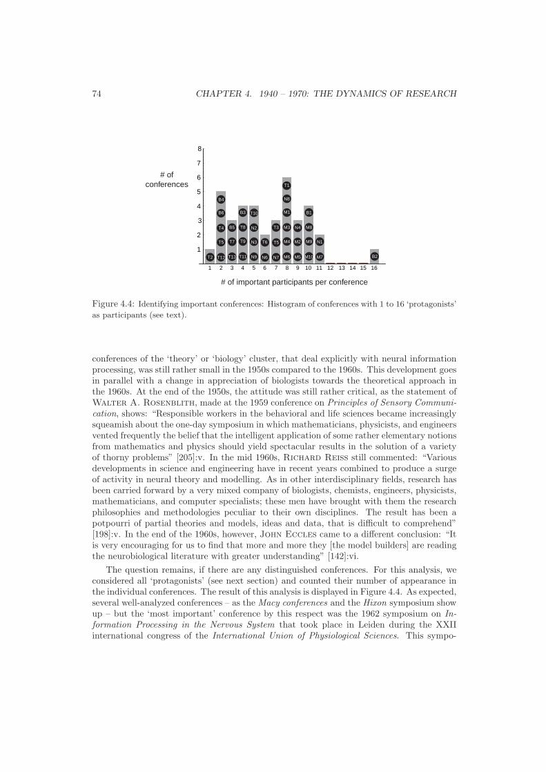
74 CHAPTER 4. 1940 – 1970: THE DYNAMICS OF RESEARCH
1 2 3 4 5 6 7 8 9 10 11 12 13 14 15 16
1
2
3
4
5
6
7
8
B2T2 M7
N1
N6
T6
N7
T3
M10
M9
M8
B1
T11
T9
T8
B3
N9
N3
N2
T10
M5
M2
N4
T13
T7
B5
M6
M4
M3
M1
N8
T1
T12
T5
T4
B6
B4
T5
# of important participants per conference
# ofconferences
Figure 4.4: Identifying important conferences: Histogram of conferences with 1 to 16 ‘protagonists’
as participants (see text).
conferences of the ‘theory’ or ‘biology’ cluster, that deal explicitly with neural informationprocessing, was still rather small in the 1950s compared to the 1960s. This development goesin parallel with a change in appreciation of biologists towards the theoretical approach inthe 1960s. At the end of the 1950s, the attitude was still rather critical, as the statement ofWalter A. Rosenblith, made at the 1959 conference on Principles of Sensory Communi-cation, shows: “Responsible workers in the behavioral and life sciences became increasinglysqueamish about the one-day symposium in which mathematicians, physicists, and engineersvented frequently the belief that the intelligent application of some rather elementary notionsfrom mathematics and physics should yield spectacular results in the solution of a varietyof thorny problems” [205]:v. In the mid 1960s, Richard Reiss still commented: “Variousdevelopments in science and engineering have in recent years combined to produce a surgeof activity in neural theory and modelling. As in other interdisciplinary fields, research hasbeen carried forward by a very mixed company of biologists, chemists, engineers, physicists,mathematicians, and computer specialists; these men have brought with them the researchphilosophies and methodologies peculiar to their own disciplines. The result has been apotpourri of partial theories and models, ideas and data, that is difficult to comprehend”[198]:v. In the end of the 1960s, however, John Eccles came to a different conclusion: “Itis very encouraging for us to find that more and more they [the model builders] are readingthe neurobiological literature with greater understanding” [142]:vi.
The question remains, if there are any distinguished conferences. For this analysis, weconsidered all ‘protagonists’ (see next section) and counted their number of appearance inthe individual conferences. The result of this analysis is displayed in Figure 4.4. As expected,several well-analyzed conferences – as the Macy conferences and the Hixon symposium showup – but the ‘most important’ conference by this respect was the 1962 symposium on In-formation Processing in the Nervous System that took place in Leiden during the XXIIinternational congress of the International Union of Physiological Sciences. This sympo-

4.3. PROTAGONISTS 75
sium, judged as an ‘experiment’ by R.W. Gerard in his opening address, indicates araise in credibility of questions of neural information processing, as,“no one has previouslyshown the temerity, nor has any congress had the courage to invite such temerity, to stagea week-long Symposium, not as an isolated unit but as part of a large Congress” [91]:3.The organizers intended to gather three different groups of scientists: neurophysiologists,behavior researchers and ‘theorists’ (modelling, system theory, computer experts and math-ematicians). The entire symposium and its discussions have been published, whereas thetranscripts have been minimally altered by the editors. The congress served as an excellentsource and has been used extensively in our detailed analysis in the previous chapter.
4.3 Protagonists
The cluster analysis of the conferences serves as a starting point for identifying scientistswhich are frequently present in the four scientific communities identified. We are interestedin the question, whether we can identify protagonists that played a major role in developingand distributing the ideas and concepts related to the ‘information processing brain’.
Methods: Using our name database of conferences, we identified all persons that par-ticipated in at least 5 conferences to obtain our set of analysis. In this set, we includedpersons, that were identified in the previous chapter as prominent researchers in ourfield of interest. These persons are A. Rapoport, H.B. Barlow, M.A. Brazier, C.
Cherry, J.P. Segundo and C.E. Shannon. We counted the number of participationsin conferences of each cluster identified using the ‘participant distance’. Persons, thatwere only present in one cluster, are called ‘cluster persons’. Persons, present in twoclusters, are called ‘border crossers’. Persons, present in at least 3 clusters are called‘ambassadors’. We furthermore checked for persons, whose multiple presence in theNRP- and biology clusters was due to the fact that they participated in the two NRP-conferences that fell in the biology cluster. Those persons represent the continuationof the NRP community into the 1970s and were neglected when identifying ‘bordercrossers’ or ‘ambassadors’. The members of the set of all ‘border crossers’ and ‘ambas-sadors’ are called ‘protagonists’. For all ‘protagonists’, their year of birth and death,the name of the institution they were affiliated longest for 1940-1960, their origin andtheir main field of work have been evaluated. For six ‘protagonists’, whose choice willbe justified in the main text, a detailed bibliometric analysis is performed using theISI Web of Knowledge database. First, the number of papers per year present in thedatabase for the period 1945 up to the death of the person as well as the number ofcitations per year for the period of 1945-2004 have been evaluated. The presence ofhomonyms has been carefully checked. Furthermore, the publications and citationsis analyzed according to the ISI subject categories in order to investigate, in whichmain fields they published and in which main fields they had the strongest impact.Categories, that contained less than 1% of the citations are excluded from the analysis(Reichard: 0.5%). The ISI subject categories refer to the journals in which a paperis published. Papers in Science and Nature, for example, are classified as ‘interdisci-plinary science’. A publication in such a journal, or a citation within a publication insuch a journal, leads to a score. As the analysis led to almost 100 subject categories inwhich the papers of the protagonists, or the people who cited them, fell, they have beengrouped to 8 classes with comparable total number of citations and with a comparablethematic connection:

76 CHAPTER 4. 1940 – 1970: THE DYNAMICS OF RESEARCH
• Neuroscience: Neurosciences.
• Biology - Systems: Anatomy & morphology, behavioral sciences, biodiversity,conservation biology, developmental biology, ecology, endocrinology, & metabolism,entomology, environmental sciences, evolutionary biology, marine & freshwater bi-ology, microscopy, oceanography, plant sciences, zoology.
• Medicine: Anesthesiology, cardiac & cardiovascular system, clinical neurology,ergonomics, hematology, medicine: general & internal, medicine: research & ex-perimental, nutrition & dietetics, obstetrics & gynecology, oncology, ophthalmol-ogy, orthopedics, otorhinolaryngology, parasitology, pathology, peripheral vascu-lar disease, pharmacology & pharmacy, psychiatry, public environmental & oc-cupational health, radiology, nuclear medicine & medical imaging, rehabilitation,sport sciences, surgery, toxicology, tropical medicine.
• Human Sciences: Communication, education & educational research, history& philosophy of science, humanities: multidisciplinary, information science &library science, management, operations research & management science, philos-ophy, psychology, psychology: applied, psychology: biological, psychology: clini-cal, psychology: experimental, psychology: mathematical, psychology: multidis-ciplinary, religion, social issues, social sciences: interdisciplinary, social sciences:mathematical methods, sociology.
• Multidisciplinary Sciences: Multidisciplinary sciences.
• Technical Sciences: Automation & control systems, computer science: arti-ficial intelligence, computer science: cybernetics, computer science: hardware,& architecture, computer science: information systems, computer science: in-terdisciplinary applications, computer science: software engineering, computerscience: theory & methods, engineering: biomedical, engineering: chemical, engi-neering: electrical & electronic, engineering: industrial, engineering: mechanical,engineering: multidisciplinary, instruments & instrumentation, materials science:multidisciplinary, robotics, telecommunications.
• Basic Sciences: Chemistry: multidisciplinary, chemistry: physical, electrochem-istry, mathematics: applied, mathematics: interdisciplinary applications, mechan-ics, optics, physics: applied, physics: fluids & plasma, physics: mathematical,physics: multidisciplinary, statistics & probability.
• Biology – Cells: Biochemistry & molecular biology, biophysics, cell biology,genetics & heredity, physiology.
The relative numbers of publications and citations, that fall in each of these eightcategories, are displayed in a ‘spider diagram’.
Our analysis has lead to the following groups of persons. In total, 32 cluster persons(results not shown), 20 border crossers (Table 4.5) and 12 ambassadors (Table 4.6) wereidentified. As expected, the cluster persons belong to either the Macy cluster (the personsof the core group) or the NRP cluster. When considering the Macy core group, we see that24 persons participated in at least 5 Macy conferences. Half of them were protagonists,indicating the strong interdisciplinary interest of those scientists. Of special interest arethe ambassadors. Although Warren McCulloch was the ‘most busy’ conference visitor,the person most evenly present in all four clusters was Donald MacKay. However, withRalph Gerard, Julian Bigelow and Heinz von Foerster, the Macy community

4.3. PROTAGONISTS 77
Macy cluster NRP cluster Theory cluster Biology cluster10: WH Pitts (T: 2) 8: TH Bullock (B: 4) 4: GA Pask (B: 1) 4: C Pfaffmann (N: 1)9: H Kluver (T: 1) 8: R Galambos (B: 2) 3: C Cherry (B: 1) 2: MA Brazier (T: 2)9: G Bateson (T: 1) 8: PA Weiss (T: 1) 3: H Quastler (M: 1)7: HL Teuber (N: 4) 5: F Morrell (T: 1) 2: A Rapoport (B: 1)6: HW Brosin (B: 1) 5: VB Mountcastle (B: 2)6: R Lorente de No (T: 1) 4: DM Wilson (B: 1)6: J von Neumann (T: 1)3: CE Shannon (N: 1)
Table 4.5: Border crossers: Persons that participated in conferences of 2 clusters. In brackets: The
number of participations in conferences of another cluster. Abbreviations: B: biology cluster, M:
Macy cluster, N: NRP cluster, T: theory cluster.
has accounted (beside McCulloch) three more persons to the group of the ambassadors.Four of the other ambassadors (Barlow, Eccles, Wall, Wiersma) were physiologistsby training, whereas the other three (Harmon, Reichard, Selfridge) descent from abasic science or engineering tradition with some affinity to biological questions (especiallyWerner Reichard).
The ‘protagonists’ repre-
sent a considerable part
of the ‘scientific elite’ of
the 1940s to 1960s.
In total, 32 persons were identified as ‘protagonists’. They representa considerable part of the ‘scientific elite’ of the 1940s to 1960s – at leastin the emerging neuroscience (e.g. Eccles, Gerard, Barlow), infor-mation and computer science (e.g. Shannon, Selfridge, von Neu-
mann), and cybernetics (e.g. McCulloch, MacKay, Pask) as well aspeople with an outstanding interdisciplinary reference (e.g. Bateson,Rapoport, von Foerster). This shows, that scientific questions re-lated to the brain, and neuronal information processing in particular were indeed of greatinterest of outstanding scientists at that time.
The classification of the protagonists according to origin leads to three results. First,25 of 32 persons originate or migrated to the USA (15 persons were born in the UnitedStates, Table 4.7). This indicates again, that the geographical origin of the ‘informationprocessing brain’ is the United States (however, our analysis did not cover any sources in
Name Macy NRP Theory Biology20: WS McCulloch 10 1 9 013: DM MacKay 1 6 4 212: RW Gerard 9 0 2 110: JH Bigelow 8 1 0 19: H von Foerster 5 0 3 16: WE Reichardt 0 3 1 25: JC Eccles 0 3 1 15: LD Harmon 0 2 1 25: OG Selfridge 0 1 3 15: PD Wall 0 2 1 25: CA Wiersma 0 1 1 34: HB Barlow 0 1 2 1
Table 4.6: Ambassadors: Persons that participated in conferences of at least 3 clusters.

78 CHAPTER 4. 1940 – 1970: THE DYNAMICS OF RESEARCH
Name Birth, death Place of work FieldJulian H. Bigelow 1897-1979 I Advanced Study, Princeton Technical ScienceMary A. Brazier 1908-1988 U California, Los Angeles NeuroscienceHenry W. Brosin ? U Pittsburg Medical ScienceTheodore H. Bullock 1915-2005 U California, San Diego NeuroscienceRobert Galambos 1914* Walter Reed Army I, Silver Spring MD NeuroscienceRalph W. Gerard 1900-1974 U Chicago Biology: cellsLeon D. Harmon ? Bell Laboratories, Murray Hill NJ Technical scienceWarren S. McCulloch 1898-1968 U Illinois (later: MIT) Biology: cellsFrank Morrell 1926-1996 Stanford U NeuroscienceVernon B. Mountcastle 1918* John Hopkins S of Medicine, Baltimore NeuroscienceCarl Pfaffmann 1913-1994 Brown U, Providence Human ScienceWalter H. Pitts 1923-1969 U Chicago Basic scienceClaude E. Shannon 1916-2001 Bell Laboratories, Murray Hill NJ Basic scienceCornelius A. Wiersma 1925-2001 CalTech, Pasadena NeuroscienceDonald M. Wilson ? U California, Berkeley Neuroscience
Table 4.7: ‘Important people’ of American origin. Abbreviations: U: University; I: Institute; S:
School. For some persons, no assured source for the date of birth and death have been found.
the Soviet Union). Second, the persons that immigrated into the US (10 in total) – mostlydue to the war induced transitions – account for a considerable part of the ‘American’scientific power in this field (Table 4.8). Third, researchers from the United Kingdom weredominant within the groups of non-Americans (Table 4.9). We choose the following sixpersons for a citation analysis: Warren McCulloch, who is the ‘ambassador’ with thehighest number of conference participations, and, as the historical analysis showed, wasinvolved in many important developments that lead to the ‘information processing brain’ –notably in neural modelling, the neuronal channel capacity discussion and the establishmentof the brain-computer analogy. Donald MacKay, who was probably the intellectually mostcomprehensive researcher within the domain, which is reflected in his various publications inmany different as well as in the fact, that we has present in conferences of all four clusters.Ralph Gerard, who was descended (as McCulloch) from the Macy tradition, was co-organizer of the important 1962 conference in Leiden and was founding member of the
Name Birth, death Place of work Field OriginGregory Bateson 1904-1980 Stanford U Human sci. UK (1939)Heinrich Kluver 1897-1979 U Chicago Biology: sys. Germany (1923)Rafael Lorente de No 1902-1990 Rockefeller I, New York Biology: cells Spain (1931?)Henry Quastler 1908-1963 U Illinois, Urbana Biology: cells Austria (1939)Anatol Rapoport 1911* U Michigan, Ann Harbor Multidisc. sci. Ukraina (1922)Oliver G. Selfridge ? MIT, Cambridge Technical sci. UK (age of 14)Hans-Lukas Teuber 1916-1977 New York U Neurosci. Germany (1941)Heinz von Foerster 1912-2002 U Illinois, Urbana Multidisc. sci. Austria (1948)John von Neumann 1903-1957 I Adv. Study, Princeton Basic sci. Hungary (1930)Paul Alfred Weiss 1898-1989 U Chicago Biology: sys. Austria (1939?)
Table 4.8: ‘Important people’, emigrants to the US. Abbreviations: U: University; I: Institute; sci:
science. The year in brackets after the country of origin indicates the time of emigration. For some
persons, no assured source for the date of birth and death have been found.

4.3. PROTAGONISTS 79
Name Birth, death Place of work Field OriginHorace B. Barlow 1921* Cambridge U Neurosci. UKColin Cherry 1914-1981 Imperial College, London Basic sci. UKJohn C. Eccles 1903-1997 Australian National U, Canberra Neurosci. AustraliaDonald M. MacKay 1922-1987 King’s College, London Human sci. UKGordon A. Pask 1928-1996 Systems Research Ltd, London Multidisc. sci. UKWerner E. Reichardt 1924-1992 MPI biol. Kybernetik, Tubingen Neurosci. GermanyPatrick D. Wall 1925* MIT (later: U College, London) Neurosci. UK
Table 4.9: ‘Important people’, non-Americans. Abbreviations: U: University; sci: science.
Society of Neuroscience. As fourth and fifth persons, we chose the two neurophysiologistsHorace Barlow and Theodore Bullock (latter is not classified as ‘ambassador’), whowere major figures in the early neural coding debate, as the historical analysis showed.Finally, we have chosen Werner Reichardt as sixth person, as he was later an importantpromotor of cybernetics in Germany and showed up surprisingly frequent in the conferenceswe investigated. We also performed a citation analysis for Heinz von Foerster. Due to thecomparatively low number of entrances in the ISI Web of Knowledge database, we excludedhim later from the analysis. The ‘ambassadors’ Bigelow, Eccles, Harmon, Selfrigde
and Wall, and Wiersma were not considered as a result of their seldom appearance in thehistorical analysis, or due to time constraints.
Protagonists – Short Biographies: We provide short biographies of the six personsidentified as ‘protagonists’:11
• Horace B. Barlow (1921*): Horace Basil Barlow was born 1921 as sonof Alan and Nora Barlow – which were part of the Darwin-Wedgwood familyand Barlow is thus the great-grandson of Charles Darwin. After gettingmedically qualified at Cambridge University, the Harvard Medical School, and theUniversity College Hospital (1947), he became a research student under Adrian
(1947-1950) in Cambridge. In the 1960s, he became professor of physiology atthe University of California in Berkeley. In 1973, he returned to England andbecame research professor in the physiological laboratory in Cambridge (he retiredin 1987). Barlow’s main field of work was visual neurophysiology, where heintroduced the concept of a ‘feature detector’ (see section 3.2.1).
• Theodore H. Bullock (1915*): Theodore Holmes Bullock was born onMay 16 1915 in Nanking, China as the son of Presbyterian missionary parents. Hemade his studies at the University of California in Berkeley, where he received hisBA in 1936 and his PhD in 1940. His appointments were at the Yale UniversitySchool of Medicine and the University of Missouri, until he got a permanentposition at the University of California in Los Angeles (1946-1966). From 1966he changed to the University of California in San Diego, where he remainedprofessor until 1982. His main field of work was invertebrate neurobiology and
11Our main sources are: Barlow: Laudatio in honor of the Australia Prize, awarded to Barlow in1993 (https://sciencegrants.dest.gov.au/SciencePrice/Pages/PreviousPrizeWinners.aspc) and the in-ternet encyclopedia Wikipedia (http://www.wikipedia.org). Bullock: His autobiography [302]. Ger-
ard: Obituary in Behavioral Science [90]. MacKay: Obituary in Nature [326]. McCulloch: dic-tionary entry of Lettvin [324] and Wikipedia. Reichardt: Obituary of the Max-Planck-Societyhttp://www.kyb.tuebingen.mpg.de/re/obituary.html

80 CHAPTER 4. 1940 – 1970: THE DYNAMICS OF RESEARCH
his two volume treatise with Adrian Horridge, Structure an Function on theNervous System of Invertebrates, became a standard textbook.
• Ralph W. Gerard (1900-1974): Ralph Waldo Gerard was born in Harvey,Illinois in 1900. He received his BS in 1919 and his PhD in 1921 at the Universityof Chicago and later, in 1924, the MD degree from the Rush Medical College. In1926 he worked in Europe (England and Germany) and returned in 1927 to theUniversity of Chicago, where he remained in the Physiology Department until1952. He then became Director of Laboratories at the Neuropsychiatric Instituteof the Medical School (University of Illinois). In 1955, he became professor ofbehavioral science. In the same year, he helped to found the Medical HealthResearch Institute at the Institute of Michigan in Ann Harbor, where he alsobecame professor of neurophysiology and physiology (1955-63). From 1963 hehelped organize the Irvine Campus of the University of California and served asdean of its Graduate Division until his retirement in 1970. His field of interestranged from neurophysiology to behavioral sciences. He had also a special interestin questions of education and teaching.
• Donald M. MacKay (1922-1987): Donald MacCrimmon MacKay wasborn in 1922. After a training in physics and a three year wartime experience inradar research, he joined in 1946 the King’s College in London, where he turnedhis attention to high-speed analogue computers and their possible relevance tothe human brain. He was among the first British scientists who appreciatedinformation theory and cybernetics in setting theoretical limits to the performanceof the human brain. In 1960, he moved to Keele University, where he founded theDepartment of Communication and Neuroscience. This institution soon became ainterdisciplinary research institute of international standing. MacKay also madeseveral philosophical contributions to the debate about free will and determinism,as well to religious questions, as he was an active churchman. He was also aneffective communicator of scientific and philosophical ideas.
• Warren S. McCulloch (1898-1968): Warren Sturgis McCulloch wasborn in Orange, New Jersey. He first studied medicine in Yale and ColumbiaUniversity in New York and received his MD in 1927. Later, he also obtaineda training in neurophysiology (1928-1931), studied mathematical physics (1931-1932) and worked as a clinician from 1932 to 1934. Then, he joined the YaleLaboratory of Neurophysiology, where he became an assistant professor in 1941.His mentor was Dusser de Barenne. In 1941, McCulloch joined the IllinoisNeuropsychiatric Institute as associate professor of psychiatry at the Universityof Illinois, where, in 1942, he took Walter Pitts as student. In the 1940sMcCulloch joined the ‘teleological society’ of Wiener and later became thechairman of the Macy conferences. In 1951, he moved his group to the MIT(Pitts was already at the MIT), where he stayed until his death. McCulloch
had many fields of interest, besides neurophysiology especially in cybernetics. Hewas founding member and first president (1967-1968) of the American Society ofCybernetics.
• Werner E. Reichardt (1924-1992): Werner Reichardt was born 1924 inBerlin. Right after his high school graduation in 1941, he was called to the Luft-waffe and served in a technical unit developing long distance radio communicationfor weather forecasts. In 1943, Reichardt joined a resistance group trying toestablish a radio contact with the Western Allies. These activities were discov-ered at the end of 1944, Reichardt was arrested and expected his execution.

4.3. PROTAGONISTS 81
Neuroscience
Biol: systems
Medicine
Human sci.
Multidisciplinary sci.Technical sci.
Basic sci.
Biol: cells
Neuroscience
Biol: systems
Medicine
Human sci.
Multidisciplinary sci.
Technical sci.
Basic sci.
Biol: cells
McCulloch
# of citations /publications
Publications
Citations:
Publications Citations
100
200
300
400
500
600
45-49
50-54
5559
60-64
65-69
70-74
75-79
80-84
85-89
90-94
95-99
00-04
10
20
30
Total
Bull Math Biophys
Difference
year
102030 10 20 30 102030 10 20 30
Axes: %
Figure 4.5: Citation analysis for McCulloch . Above, the number of citations (all papers, only
[159], difference between both) and the number of publications per 5-year-period since 1945 (note
that the number of publications in the graph is scaled with 10 to increase visibility). Below, the
classification of the publications of McCulloch and the citations of his work. The distribution of
the citations of the McCulloch-Pitts paper is indicated by the grey line (unfilled area).
In the last days of the Nazi regime he managed a narrow escape during a rebel-lion of prisoners and could hide himself in Berlin until the end of the war. Afterthe war, Reichardt studied physics at the Technical University in Berlin andfinished his studies with a doctoral thesis in solid state physics in 1952. In the1950s, he started to work with the visual system of insects. In 1954, he was in-vited by Max Delbruck to the California Institute of Technology in Pasadena.Back to Germany, Reichardt became in 1955 Research Assistant at the MPI furphysikalische Chemie in Gottingen. In 1958, a research group for cybernetics wasestablished at the MPI fur Biologie in Tubingen. In 1960, he became professor inTubingen. A separate building for his department was opened in 1965 and wastransformed into the Max-Planck-Institute fur biologische Kybernetik in 1968.
The bibliometric analysis for the six protagonists shows a more detailed picture (note,that in the graphs the number of publications are scaled with 10 to increase visibility). Itis clearly visible, that the results of the citation analysis of the ‘Macy-persons’, McCul-
loch (Fig. 4.5) and Gerard (Fig. 4.6) are very different, although they worked in quite
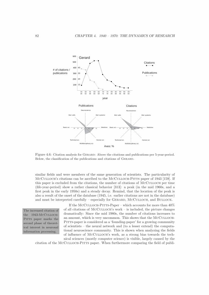
82 CHAPTER 4. 1940 – 1970: THE DYNAMICS OF RESEARCH
Gerard
# of citations /publications Publications
Citations
year
Neuroscience
Biol: systems
Medicine
Human sci.
Multidisciplinary sci.
Technical sci.
Basic sci.
Biol: cells
Neuroscience
Biol: systems
Medicine
Human sci.
Multidisciplinary sci.
Technical sci.
Basic sci.
Biol: cells
Publications Citations
100
200
300
400
500
600
45-49
50-54
5559
60-64
65-69
70-74
75-79
80-84
85-89
90-94
95-99
00-04
10
20
30
40
102030 10 20 30 102030 10 20 30
Axes: %
Figure 4.6: Citation analysis for Gerard: Above the citations and publications per 5-year-period.
Below, the classification of the publications and citations of Gerard.
similar fields and were members of the same generation of scientists. The particularity ofMcCulloch’s citations can be ascribed to the McCulloch-Pitts paper of 1943 [159]. Ifthis paper is excluded from the citations, the number of citations of McCulloch per time(fife-year-period) show a rather classical behavior [313]: a peak (in the mid 1960s, and afirst peak in the early 1950s) and a steady decay. Remind, that the location of the peak isalso a result of the onset of the database (1945, i.e. earlier citations are not in the database)and must be interpreted carefully – especially for Gerard, McCulloch, and Bullock.
The increased citation of
the 1943-McCulloch-
Pitts paper marks the
second phase of theoret-
ical interest in neuronal
information processing.
If the McCulloch-Pitts-Paper – which accounts for more than 40%of all citations of McCulloch’s work – is included, the picture changesdramatically: Since the mid 1980s, the number of citations increases toan amount, which is very uncommon. This shows that the McCulloch-Pitts-paper is considered as a ‘founding-paper’ for a growing communityof scientists – the neural network and (to a lesser extend) the computa-tional neuroscience community. This is shown when analyzing the fieldsof influence of McCulloch’s work, as a strong bias towards the tech-nical sciences (mostly computer science) is visible, largely caused by the
citation of the McCulloch-Pitts paper. When furthermore comparing the field of publi-

4.3. PROTAGONISTS 83
Barlow
# of citations /publications
Publications
Citations
Neuroscience
Biol: systems
Medicine
Human sci.
Multidisciplinary sci.
Technical sci.
Basic sci.
Biol: cells
Neuroscience
Biol: systems
Medicine
Human sci.
Multidisciplinary sci.
Technical sci.
Basic sci.
Biol: cells
Publications Citations
200
400
600
800
1000
1200
1400
45-49
50-54
5559
60-64
65-69
70-74
75-79
80-84
85-89
90-94
95-99
00-04
2010
year
102030 10 20 30 102030 10 20 30
Axes: %
Figure 4.7: Citation analysis for Barlow. Above the number of citations and publications per
5-year-period. Below the classification of publications and citations according to different fields.
cation activity with the field of citation, one sees that the publications of McCulloch inMedicine (the field with the largest fraction of McCulloch’s publications) is not stronglyacknowledged. The peak in the field ‘multidisciplinary’ in the publications when comparedwith the citations is a general phenomena, that is also visible when looking at other protag-onists. This results from publications in interdisciplinary journals (e.g. Nature or Science),which usually are not again cited in a publication of a multidisciplinary journal, but mostlyin special journals. Furthermore, publications in interdisciplinary journals are used to pro-mote own work, such that citations in such contributions often refer to work published inspecialized journals.12 Because of that effect, the number of publications in the field ‘multi-disciplinary science’ is usually larger than the number of citations in that field. The graph ofthe citation analysis of Gerard shows a classical course: a peak in the mid 1960s, followedby a decay in citations. Also when the fields of publication are compared with the fields ofcitations, a much more regular picture emerges, as Gerard was recognized basically in thesame fields where he published. An exception is his work in psychology (human sciences),which is obviously less well recognized than his work in cellular biology and medicine.
12Urs Schoepflin, MPI for the History of Science, Berlin: personal communication.

84 CHAPTER 4. 1940 – 1970: THE DYNAMICS OF RESEARCH
Bullock
# of citations /publications
Neuroscience
Biol: systems
Medicine
Human sci.
Multidisciplinary sci.
Technical sci.
Basic sci.
Biol: cells
Neuroscience
Biol: systems
Medicine
Human sci.
Multidisciplinary sci.
Technical sci.
Basic sci.
Biol: cells
Publications Citations
200
400
600
800
1000
45-49
50-54
5559
60-64
65-69
70-74
75-79
80-84
85-89
90-94
95-99
00-04
20
10
Publications
Citations:
Total
"Structure and ..."
Difference
102030 10 20 30 102030 10 20 30
Axes: %
Figure 4.8: Citation analysis for Bullock. Above the number of citations and publications per
5-year-period. Below the classification of publications and citations according to different fields.
The two biologists of the protagonists investigated – Barlow and Bullock – showthe highest number of citations in general. This indicates a different citation culture inbiology when comparing with other fields. There are, however, some interesting differences:Almost a quarter of Bullock’s citations emerge from his well-known standard monographStructure and function in the nervous systems of invertebrates [52], which appeared in 1965and was very soon acknowledged in the community (Fig. 4.8). Barlow, on the other hand,has various, well-cited publications, but no single publication that accounts for a significantamount of the total number of citations (Fig. 4.8). Barlow furthermore publishes not manypaper per year – but when he publishes, it is usually well-acknowledged in the community.The citations increase considerably in the mid 1960s, indicating that Barlow became aprominent scientist in that period. The fact that Barlow’s citations usually fall in the cat-egory neuroscience (which is a modern category), together with the still not decreasing curveof citations, indicate, that he is still well acknowledged in neuroscience today. Bullock’sincreasing importance in the mid 1960s is basically ascribed to his monograph, although afirst increase in importance is already visible at the beginning of the 1960s. He furthermoreshows the most stable publication-citation comparison concerning the distribution of cita-tions within categories. Whereas Barlow’s work has some impact in the technical sciences,

4.3. PROTAGONISTS 85
Neuroscience
Biol: systems
Medicine
Human sci.
Multidisciplinary sci.
Technical sci.
Basic sci.
Biol: cells
Neuroscience
Biol: systems
Medicine
Human sci.
Multidisciplinary sci.
Technical sci.
Basic sci.
Biol: cells
# of citations /publications
Publications
Citations
Publications Citations
102030 10 20 30102030 10 20 30
Axes: %
100
200
300
400
500
600
45-49
50-54
5559
60-64
65-69
70-74
75-79
80-84
85-89
90-94
95-99
00-04
year
10
20
30
40
Figure 4.9: Citation analysis for MacKay: Above the number of citations and publications per
5-year-period. Below the classification of publications and citations according to different fields.
human sciences and medicine as well, the work of Bullock is restricted to the biologicalsciences.
The two multidisciplinary European scientists – MacKay and Reichardt – display alsointeresting differences in the citation analysis. For both, the absolute numbers of citationsare considerably smaller than those of Barlow and Bullock. At least for Reichardt, thisdifference may reflect the bias of the ISI-database towards American and English journals, asa considerable part of his publications are not contained in the ISI database, which distortsthe citation analysis.13 The citation analysis of MacKay shows a peak in the mid 1970s,the same time he also published the most (Fig. 4.9). His citations decay slowly, indicating,that he is still rather influential. MacKay shows publication activity in all fields, whichdemonstrates his broad interdisciplinary interest. He is most cited in the category humansciences (especially in psychology). Reichard’s citations, finally, show the slowest increaseof all six protagonists (Fig. 4.10). His citations reach a peak in the early 1990s (after his
13The official website of the Max-Planck-Society (http://www.kyb.mpg.de/∼wreichardt) lists 70 journalarticles, 27 conference papers, 24 book chapters and 5 popular scientific publications. The ISI Web ofKnowledge database contained 59 entries. Conference proceedings, popular science publications are, how-ever, usually not contained in the database. Concerning the analysis of Reichardt’s work, the number ofhomologes was quite large and needed a considerable amount of work to check individual entries.

86 CHAPTER 4. 1940 – 1970: THE DYNAMICS OF RESEARCH
Reichardt
year
# of citations /publications
Publications
Citations
Neuroscience
Biol: systems
Medicine
Human sci.
Multidisciplinary sci.
Technical sci.
Basic sci.
Biol: cells
Neuroscience
Biol: systems
Medicine
Human sci.
Multidisciplinary sci.
Technical sci.
Basic sci.
Biol: cells
Publications Citations
102030 10 20 30 102030 10 20 30
100
200
300
400
500
600
45-49
50-54
5559
60-64
65-69
70-74
75-79
80-84
85-89
90-94
95-99
00-04
10
20
Axes: %
Figure 4.10: Citation analysis for Reichardt. Above the number of citations and publications
per 5-year-period. Below the classification of publications and citations according to different fields.
death). The analysis of Reichardt’s publications according to category shows a ‘double-peak’ characteristic for interdisciplinary work, as he published in neuroscience as well as intechnical science journals. His major impact, however, lies in the biological sciences.
4.4 Synopsis: Qualitative and Quantitative Analysis
We conclude the historical analysis by a synopsis, where we integrate the results of thehistorical (qualitative) and scientometric (quantitative) analysis. We shortly review thepreconditions of the ‘information processing brain’ that there established until the 1930s,summarize the main developments in the 1940s to 1960s and list the open achievements andquestions, that were set at the beginning of the 1970s. Figure 4.11 provides an overview.
4.4.1 Up to 1940: Preconditions
The conceptualization of the ‘information processing brain’ needed a clear picture of theactivity on the micro scale, in order that an entity is able to perform the ‘processing’ and

4.4. SYNOPSIS: QUALITATIVE AND QUANTITATIVE ANALYSIS 87
1920s1930s
1940s
1950s
1960s
Early modelling
Emergence of thespike / spike train
Neural variability& active brain
Conceptualizationof information
Use ofinformationvocabulary:
neural channel
neural code
Searchfor
biological(neural)
information
&
How usefulis information
theory?
Growingnumber of
neural models
&
Emergenceof the
brain-computeranalogy
Growingnumber of
candidate codesGrowing
doubts oninformation-approach
Bionicinspiration
No definitionof "neural
information"
No stabilizedconcept of
"neural code"
Singleneurondoctrine
definedstatistical
toolset
Findingnew roles
for neurons
Determiningelements ofvariability:
neural noise&
network-connectivity
How does reliabilityemerge out of
unreliable elements?
Consequencesof neuronalvariability
Development of statisticaltoolbox forspike trainanalysis
McCulloch-Pitts-model
New instruments
Unclearrole of"neuralnoise"
Neuron doctrine
Figure 4.11: An overview of the main historical developments, that lead to the notion of the
‘information processing brain’ in the 1940s to 1960s.
another entity is able to represent the ‘information’. The first aspect – the neuron as ba-sic processor – was based on the neuron doctrine, which at that time was sufficiently firm(although not proven) to serve as justification. The second aspect needed the emergence ofthe single, ‘digital’ spike and the spike train, that can be measured reliably. The spike trainand his mathematical abstraction (as series of event-times or ‘interspike intervals’) then canserve as a bearer of information that is accessible for further (theoretical) analysis. The cre-ation of the spike train required instruments that were able to measure and store the spikes.The American physiologists Forbes, Gasser and Erlanger and the British physiologists

88 CHAPTER 4. 1940 – 1970: THE DYNAMICS OF RESEARCH
Lucas and Adrian were prominent among those scientists, that enabled this development.Adrian had furthermore a distinguished role, as he described the neural communicationproblem comprehensively and by using the concept of a ‘message’ that nerve fibres trans-mit. The establishment of the spike train was, however, not unproblematic. Improvementsin measuring spikes, e.g. by Pecher, also showed an intrinsic variability of neuronal firing,that can no more be attributed to unreliable instruments. Furthermore, the mass actionhypothesis of Lashley advanced the perspective of a ‘active brain’, whose elements (theneurons) are capable of spontaneous activity. From a technical point of view, these aspectsmake the neuron ‘unreliable’. This had two important consequences for the later develop-ment: First, the ‘unreliable neuron’ hampered the application of the information vocabularyas it was unclear, to what extend one can understand the variability as resulting from noise.Second, the ‘unreliable neuron’ also served as an inspiration for technology development,which was recognized very early – notably by McCulloch and von Neumann – and thequestion emerged, how one could build reliable machines out of unreliable components.
In the 1930s, neurons and the brain also became object of a rigid mathematical approachin order to model their behavior. A protagonist in this respect was Rashevsky, whose pro-gram of mathematical biophysics, especially in the field of cell and molecular biology, laterwas discredited as being too theoretical and lacking empirical grounding. In neural mod-elling, however, he (and later his students) insisted on the use of a continuous mathematicsinstead of the discrete approach of McCulloch/Pitts. In this sense he was more prudentin respect of the mechanization of neural processes. Furthermore, he later supported the sta-tistical approach in respect of neural connectivity. We therefore suppose, that Rashevsky
can be considered as one precursor of today’s dynamical systems and statistical physics ap-proach towards the modelling of neural systems, although the McCulloch/Pitts modelhad a much larger appreciation within the theoretical community at that time (and now).
4.4.2 1940-1970: Main Developments
A first important step towards the information processing brain was the conceptualization ofinformation, which included the emergence of information theory and cybernetics. However,not all of the persons identified as main protagonists in this respect – Warren McCulloch,Walter Pitts, Claude Shannon, Alan Turing, John von Neumann and Norbert
Wiener – were equally important in the following historical developments. McCulloch
was a decisive figure in the whole development due to several reasons: First, as shownby the bibliometric analysis, he introduced together with Pitts a very influential neuralmodel based on the ‘digital character’ of the spike and the neuron doctrine, especiallyfor the ‘second phase’ of interest in theoretical questions of neural information processing(since the 1980s). Second, he was chairman of the Macy conferences. Although questionsof neural information processing were not in the focus of this conference series, the Macydiscussions anticipate several aspects, like neural coding and the technical implications ofneuronal information processing, that later became important. Third, as our cluster analysishas shown, McCulloch was a busy ambassador of his ideas, especially in the theoreticalneuroscience community. Also von Neumann was an important figure, as a shift of his focustowards problems of neural information processing emerged since the 1940s. In particular, hetook the inspirational value of neuronal information processing for technological systems veryserious (much more than McCulloch) and developed a precise framework to study these

4.4. SYNOPSIS: QUALITATIVE AND QUANTITATIVE ANALYSIS 89
questions within the emerging automata theory. His contributions at the Macy discussionsdemonstrate a prudent and sophisticated approach towards questions of neural coding. Thework of Pitts is more difficult to judge, as much of his work has been destroyed. Itseems that he was interested in a ‘statistical physics’ approach towards processes in neuralsystems, which undoubtedly would have been an innovation at that time. He was, however,not present in many different communities and, besides the McCulloch/Pitts paper, notan influential person, especially within the biological community. Shannon shows up in ouranalysis in two respects (besides being the ‘founder’ of information theory): First, he wascritical towards an extended application of information theory, although his critique mainlyfocussed applications towards human systems, where semantics is inevitable. Second, heshowed an interest in questions of biological information, which is shown in his later work onbuilding ‘intelligent artefacts’ and his participations at biological conferences. Wiener andTuring, finally, do not show up in our analysis to a relevant degree. They supposedly failedto gain any involvement in the ‘neural coding’ and ‘neural information processing’ discussion,although Wiener can be considered as the founder of the brain-computer analogy. However,one has to keep in mind that we did not discuss the development of artificial intelligence,where Turing was a more important figure.¡
The conceptualization of information promoted several new fields of discussion: Thefirst concerns the application of the information vocabulary on neural systems, exemplarilyshown in the work of Barlow and FitzHug in the visual system in the 1950s. At thesame time, a discussion on neural channel capacity emerged, promoted by McCulloch,MacKay and Rapoport. This discussion was entangled with the question, which ‘code’a neuron may use. Together with the assumption of ‘information capacity maximization’(proposed by McCulloch), the field for new, temporal, codes was open. One example is the‘pattern code’, that was found to be an attractive theoretical concept (e.g. by Rapoport
and Harmon) and found support by experiments performed by Wiersma. In the late 1950sand early 1960s, several conferences – among them the 1962 Leiden conference organized byGerard – discussed this matter. In that time, the neural coding debate had his first peak –some important persons in this respect are Barlow, Bullock, Mountcastle, Segundo
and Uttal. Unlike the discussion about the genetic code (that happened at the same), nostabilized concept of a ‘neural code’ emerged, rather an explosion of candidate codes wasvisible – exemplified in the NRP work session on neural coding of 1968.
Another field of discussion can be grouped around the concept of ‘neural information’.In the early 1950s, this discussion was already resumed in the field of molecular biology(Quaster), where it lead to a disappointing result. The discussion of the concept of neuralinformation – by Brazier, MacKay and Rapoport and others – had a similar faith: agrowing scepticism within the neuroscience community towards the useability of informationtheory within their field. The same scepticism also emerged towards the brain-computeranalogy, that was further developed in the 1950s in the cybernetic (and artificial intelligence)community (e.g. by Ashby and George). More and more, however, it was clear that thisanalogy should not be used to explain the brain (although for example the Perceptron hasbeen introduced by Rosenblatt for exactly that purpose), but to find new technology. This‘bionic inspiration’ was first formulated by McCulloch and von Neumann and pushedforward especially by von Foerster.
A recalcitrant problem was neuronal variability that inspired the search for neuronal noisesources (e.g. by Fatt/Katz, and later by Verveen/Derksen and Calvin/Stevens). It

90 CHAPTER 4. 1940 – 1970: THE DYNAMICS OF RESEARCH
also led to a growing importance of statistical aspects in respect of neuronal connectivity.For the modeler community, a new challenge was born, as one had to assess, whether theseaspects of randomness still allow a stable systems behavior. For the neurophysiologist,on the other hand, two problems emerged: First, a new need for statistical tools thatallow the handling of variability emerged. This led in the 1960s to the development andconsolidation of a statistical toolbox for spike train analysis (Gerstein, Moore, Perkel,Stein). Second, a dispute about the consequences of neuronal variability for measuringneuronal activity emerged: One side argued, that only the mean response of a neuron canbe considered as relevant – for the experimentalist and for the neuron (Burns), whereasothers refuse the notion of ‘neuronal unreliability’ (Barlow, Bullock). Latter standpointwas successful in the sense that it was able to formulate a new role for neurons as ‘featuredetector’, leading to the single neuron doctrine. In this field of discussion, also a newstandpoint emerged that criticized the usage of the term ‘noise’ as a disturbing element.Rather, it was argued, that noise in biological systems might indeed have a functional role,although no consensus emerged, what this role could be.
In summary, the situation in the early 1970s led to the following specification of theinformation processing brain: The information vocabulary has been introduced and ‘tested’within the context provided by the emerging neuroscience. Scientists that investigatedexplicitly the signal processing properties of neuronal systems started to use terms like‘neural code’, ‘neural information’ or ‘neural noise’. In that sense these concepts became partof the vocabulary of neuroscience. However, the ‘test’ of these terms also showed that precisedefinitions in the sense of information theory were not practicable within neuroscience.Alternative and generally accepted concepts were not found, rather an increasing numberof proposals (especially for a ‘neural code’) made it necessary to use these concepts in ametaphorical sense and not as precisely defined scientific concepts. The turn from the 1960sto 1970s marks the end of a period, where a first attempt to integrate and conceptualizethe information vocabulary within neuroscience has been made. However, at the end of the1960s, a large variety of models as well as a mathematical toolbox for spike train analysiswas available. This allowed a steady but slow growth of those fields of neuroscience wherethe development of theoretical concepts that describe the information processing propertiesof the brain was in the focus. This growths increased markedly in the mid 1980s, leadingto a ‘second phase’ of interest in the theoretical investigation of the information processingbrain. Although we did not investigate this point in detail, we suspect that the increasedpossibilities of computational modelling was a major driving force for this development.In this development, physicists and computer scientists that had a much larger affinity tothe information vocabulary entered neuroscience. This also enforced the interest in findingmore precise definitions for ‘neural information’, ‘neural code’ or ‘neural noise’. Up to now,however, a ‘success’ in this respect has not been reached.

Part II
Patterns in Neuronal SpikeTrains
91


Chapter 5
Neural Coding andComputation
This chapter sets a general framework for the spike pattern discussion by defining
the terms ‘neural coding’ and ‘neural computation’. We start from the finding
that the early neural coding debate did not solve the coding problem. We list the
main difficulties that appear when the concepts ‘code’ and ‘computation’ are used
to denote processed in neural systems and present a definition of both terms.
5.1 Neural Coding
5.1.1 What is a ‘Neural Code’?
A code defines the possi-
ble sequences of inputs,
outputs and their inter-
relation.
When referring to processes performed by neurons, the terms ‘coding’and ‘computation’ are widely used in today’s (theoretical) neuroscience[443, 651]. As our historical analysis suggests, we distinguish two phaseswhere ‘neural coding’ and ‘neural computation’ became (more) intensivelystudied topics of neuroscience. The first phase (1940s to early 1970s)ended without obtaining any generally accepted concept of a ‘neural code’or ‘neural information processing’. In the second phase (starting in themid 1980s), the situation has not changed fundamentally. Although the brain-computeranalogy of the early days of the neural coding debate is no more considered as adequate fordefining these terms precisely [544]:98, neural coding is still an important issue. On the otherhand, some believe that the terms ‘code’ and ‘computation’ are inadequate for describingneural processes [296]:153,167; [517, 336]. Any such conclusion depends on the definitionof the terms involved. We first focus on the term of a ‘neural code’. It is undisputedthat the meaning of ‘code’ in the sense of codification (a legal term) or in the sense of acomputer code (a symbolic arrangement of data or instructions in a computer program) do
93

94 CHAPTER 5. NEURAL CODING AND COMPUTATION
not apply when using the term ‘neural code’. As shown in chapter 3, the term ‘neural code’appeared in neuroscience after the introduction of Shannon’s scheme of a communicationsystem (see Fig. 2.1) [227], although the term usually has not been used in the precisedefinition of a (discrete) transducer proposed by Shannon. In the mathematical notationof Kolmogorov [133], the communication scheme is translated into a chain of operationsξ → η → η′ → ξ′, where η → η′ stands for a transmitting device, ξ → η for a codingoperation and η′ → ξ′ for a decoding operation (ξ stands for a message and η stands fora signal). Any such communication process can only operate (and be observed) with finiteprecision. Whatever entities ξ and η are composed of, in the act ob observing them weattribute numbers or other types of symbols to them. In that sense, the most generaldefinition of a code is that of a relation between sets of symbols [437]. We define:
Definition 5.1 A countable set of symbols A = a1, a2, . . . is called alphabet. A finite,arbitrarily arranged string of symbols of length l (ai, ai+1, . . . , ai+l) from an alphabet A iscalled word.1
Definition 5.2 For two alphabets A, B, a mapping fc : A → B relating words of A withwords of B is called code relation. If fc is injective, the code relation is called non-degenerative, if fc is bijective, the code relation is called uniquely decodable.
Definition 5.3 For two alphabets A, B and a code relation fc : A → B, we call the set ofall words of A that can serve as input for fc the code input set I and the set of all words ofB that can form the image set of fc the codeword set C.
Definition 5.4 For a code input set I, a codeword set C and a code relation fc, the triplet(fc, I, C) is called code.
This definition is very general and applies for any relationship between two entitiesdescribed by two sets of symbols. The term ‘symbol’ refers here in most cases to measurementvalues that provide information about the state of the system. Thus, the alphabet is formedby rational numbers. The main point is that analyzing processes in a natural system in theframework of a code consists in determining fc together with I and C. This is the reason,why not only fc (as for example proposed by [652]), but the whole tripled should be calledcode.2 The question is now: how are fc, I, and C determined?
In linguistics and semiotics, three restrictions hold for a justified application of the term‘code’: First, symbols are a special type of signs whose meaning can only be understood byincorporating the interpreter of the symbol and the conventions that attribute certain entitiesto a symbol.3 Second, fc is the result of in principle arbitrary and modifiable conventions[296]:167. Third, the rules used to relate phrases of I and C do not only have a syntactic,
1Note, that the indices i of ai within the word denotes the position of the symbol in the word and notthe number of the symbol in the alphabet. The same symbol can appear several times in a word.
2We follow the proposal of Uttal, according to which a code consists of sets of symbols used to representmessages (patterns of organization) and the set of rules that govern the selection and use of these symbols[249]:208. Some remarks to the use of the terms ‘encoding’ and ‘decoding’: Former mainly refers to sensorysystem (a stimulus is encoded), whereas latter is usually used in the sense of ‘cracking the code’.
3Several different interpretations of the concept of symbol exist: In the typology of Charles Sanders
Peirce, signs are classified as icon, index and symbol, whereas the latter is characterized by a purely arbitraryattribution between the entity and the symbol that stands for this entity.
5.1. NEURAL CODING 95
but also a semantic and pragmatic character [308]:57-61. The linguistic notion of a codeassumes the existence of a well-known language that serves as a foundation for defining thecode by its users (i.e. the attribution of phrases from I to C). From this perspective, singleneurons or groups of neurons lack principal arbitrariness of choosing a specific code relation.Furthermore, the semantic and pragmatic character of neural signals as well as the existenceof symbols, the ‘symbol restriction’, are (in the best case) unclear. Therefore, linguists andsemiotics refuse the notion of a ‘code’ when referring to neural systems [308]:31.
However, it is not compulsory to give up the notion of a ‘code’ when one is unable to fulfillall restrictions formulated above. If we agree that information theory is ‘allowed’ to used theterm code, then semantic and pragmatic constraints can be neglected. On the other hand,syntactic constraints are present due to the physical structure of the system performing thecode relation that sets some limits upon the succession of states, e.g. due to the inertia ofthe system, and thus restricts the set of possible sequence of symbols (i.e. measurementvalues). The term ‘symbol’ is furthermore used much more ‘liberal’ in information theory,referring to the signs used to represent messages. In the following, we use this broadermeaning of ‘symbol’. The second restriction, the requirement of arbitrariness, cannot beneglected completely. When a communication system is constructed, fc can indeed bechosen arbitrarily to some degree so that the system is able to fulfill a certain purpose –e.g. to maximize channel capacity or to hide encoded information (cryptography). If therestriction of arbitrariness would be given up completely, the use of the term ‘code’ becomesmeaningless. Otherwise, one could say that a falling stone ‘encodes’ a certain height at time tin a certain speed at time t. The system that ‘codes’ for something must have a certain degreeof freedom in respect to relate the input with its output. At that point it is important tomention that the physical process which performs the code relation (the code transformation,see below) is not arbitrary at all, but has to be as deterministically as possible in order toprovide a reliable coding. The question is now: what degree of arbitrariness in determiningfc is allowed? The answer to this question is provided by analyzing the history of the system.The ‘genetic code’ serves as an example: Here, arbitrariness means that there is no chemicalnecessity that determined which nucleotide tripled codes for which amino acid. In genetics,the emergence of this relation is considered as a ‘frozen accident’. But the physical process,that relates a specific nucleotide triplet to a specific amino acid is chemically determined bythe tRNA molecule. The degree of arbitrariness is very low, as the system cannot change therelation any more after the ‘frozen accident’ happened. If the fact that the ‘frozen accident’could have happened different, is considered as a sufficient degree of arbitrariness, the useof the term ‘code’ for the genetic code is justified. Also under this assumption the geneticcode should not be mistaken for a code in the linguistic sense.
Is a certain degree of arbitrariness also fulfilled for a ‘neural code’? In other words: is thesystem able to change the input-output-attribution over time? The answer to this questiondepends on the spatial and temporal scale of the analysis: If, for example, a single synapseis considered and the input string is a time series of the number of transmitter moleculessecreted by the synapse in a small time unit and the output string is a series of values of thepost-synaptic membrane potential, then the relation is fully determined up to a stochasticmoment given by diffusion processes and channel gating. On a larger spatio-temporal scale,however, effects like adaption and long-term potentiation serve as a basis for arbitrarinessin the sense that there is no temporally invariant mapping from a given stimulus intensityto a resulting spike train [312]. We propose that this degree of arbitrariness is sufficient not

96 CHAPTER 5. NEURAL CODING AND COMPUTATION
to exclude the notion of a ‘neural code’ a priori. To discuss the ‘symbol restriction’ in aneural code, we introduce the type-token distinction, that originates from the logician andphilosopher Charles Sanders Peirce [174]:
Definition 5.5 The type of a symbol (word) denotes the abstract entity that represents thesemantic content of the symbol (word). We use the term represent to denote the relationbetween a type and its semantic content.
Definition 5.6 The token of a symbol denotes the physical entity that stands for the symbol.We use the word realize to denote the relation between a token and a type. We call the tokenswhich realize the symbols of the code input set the input tokens and the tokens which realizethe symbols of the codeword set the output tokens.
Definition 5.7 If input tokens and output tokens are given, we call the physical process tcthat transforms input tokens in output tokens the code transformation.
An event is a significant
moment in time that is
represented by a symbol.
In a technical coding context, the type-token relation is unambiguous,as the code is constructed on the type level in order to serve its purposedefined on the semantic level. Later, the tokens are chosen such thatthe realizations of phrases and codewords is reliable given the noise of thesystem. The ‘semantic’ aspect refers to the functional value of the phrasesand codewords (see Fig. 5.1). When – as in neuronal systems – one does
not construct the code but one analyzes whether a certain process can be understood as acode, the problem gets more complicated. One has to answer the question, whether tokenscan be identified in neural processes to which symbols can be attributed. This problem isrelated to the fundamental challenge for explaining neural mechanisms: how to decomposethe central nervous system into functionally meaningful parts [337]:49. This decompositioninvolves a spatial aspect (e.g. expressed by the localization debate) and a temporal aspect.Latter involves the search of certain entities that express significant moments in time withinthe processes of the system. We call these entities events, which are represented by symbols.Note, that the term ‘event’ can correspond to either a token (a specific event in space-time) or a type. In other words, there must be a natural coarse-graining of the parameterunder investigation. One may certainly argue that the measurement itself produces a coarse-graining, as the measurement resolution is finite. Each single measurement point, however,stands probably not for a significant event of the system. One has to find a way to separatethe significant events from all other phenomena that can be measured at some level oforganization in the brain. These events are then related to symbols.
The spike is the ‘classical event’ that serves as a basis for analyzing neuronal processes ina coding framework [651] (see section 2.3.3). The ‘all-or-none’ character of spikes made themcandidates for a symbolic description – e.g. by using the symbol ‘123’ to indicate that a spikeoccurred 123 ms after a certain reference point in time. Three objections have been raisedthat question spikes as basic entities for discussing neural coding: A theoretical objectiondenying the possibility that spikes may serve as symbols; an empirical objection referring toother possible tokens that may serve as basis for defining symbols; and a practical objectionstating that the determination of spike trains based on measurements (the spike sortingproblem) is not sufficiently reliable. We shortly discuss the first two problems. For the thirdproblem we refer to section 6.1.2.

5.1. NEURAL CODING 97
Stimulus Response
Codeinput set
Codewordset
Inputtokens
Outputtokens
fc
tc
Type level
Token level
Semantic level
realize
represent
cons
truc
t a c
ode a
code
deco
de
Figure 5.1: The several dimension of a code relation in natural systems: The semantic level defines
the experiment in which a stimulus is presented to the system in order to get a certain response.
The type level is the level where the definition of a code is applied. The physical processes that
realize the code happen on the token level.
The first objection claims, that spikes cannot be symbols due to two reasons [336]:First, spike times are continuous variables. Thus, the number of possible spike events isuncountable and one is not able to relate spike times with a countable alphabet. Second,the assumption that single spikes are functionally significant is unwarranted. The firstarguments reminds of the dispute between McCulloch and Rapoport, whether a real-valued or a discrete mathematics should be used in order to model neural systems (seesection 3.2.2). This distinction, however, misses the point. The problem is rather, if acoarse-graining on the temporal micro-scale is present or not. If it is present, it will show upalso using a real-valued mathematics. McCulloch and Pitts assumed an universal coarsegraining when presenting their model in 1943 (the synaptic delay) – which is certainly ashortcoming. However, although synaptic delays or spike-widths are variable, they are notarbitrary small – a coarse graining is thus possible. Furthermore, measurements involvea finite sampling rate. The ‘empirical world’ in which measurements are performed andtheories are tested is thus always a ‘discrete’ world. The argument, whereby the singlespike is not functionally significant, is an empirical question – but does not affect the morefundamental problem whether one can relate a single spike with a symbol or not. Spikesmight just not be the relevant tokens. Indeed, other events within spike trains have beenproposed to be relevant, e.g. bursts, local firing rates etc. (see section 6.1.2). All these events,however, are characterized using the spike-times of the individual spikes. In that sense, thesymbolic representation of the spike train as sequence of event-times is a prerequisite indeedfor analyzing the problem. We thus consider the first objection as unsupported. The secondobjection, the possibility that other tokens than spikes – like local field potentials [408]or neurochemical aspects [343] – are more relevant for understanding a code relation is arelevant point. This aspect, however, has to be decided empirically and is not a fundamentalargument against the role of spikes in a coding relation. We will in the following restrict

98 CHAPTER 5. NEURAL CODING AND COMPUTATION
0 0 0 0 0 0 0 0 0 01 1 1x1 x2 x3
t1 t2 t3
t = 0 t = T
Raw data
timing representation
interval representation
bitstring representation
spike threshold
time
∆τ
Figure 5.2: Different representations of spike trains: Raw data (in this picture, no real data
are displayed) is given as voltage per sampling time unit (symbolized by dots). By defining a
spike threshold, a spike train is obtained in the timing representation t1, t2, t3 and the interval
representation x1, x2, x3. After choosing a bin-with ∆τ , one obtains the bitstring representation.
ourselves to spikes as the fundamental event in order to discuss the neural coding problem.The recording of spikes leads to the notion of a ‘spike train’:
Definition 5.8 A sequence of points in time t = (t1, . . . , tL) indicating the occurrence ofspikes attributed to a single neuron of length L is called spike train.
A spike train according to Def. 5.8 is in the timing representation. An equivalent represen-tation of a spike train is given by the sequence of interspike intervals (ISI): x = (x1, . . . , xL),where xi = ti−1 − ti (x1 is the time interval from the beginning of the measurement to thefirst spike) – the interval representation. Usually, spike trains are analyzed in the timingor the interval representation. Another form of representation is obtained by transformingthe spike train t = t1, . . . , tL into a bitstring – the bitstring representation – a standardprocedure for applying methods of information theory [74]. For this transformation, themeasurement interval [0, T ] is partitioned into n bins of width ∆τ (n∆τ = T ). If at leastone spike falls into the i-th bin, the letter ‘1’ (and otherwise the letter ‘0’) is written at thei-th position of the string. Usually, ∆τ is chosen so that maximally one spike falls into onebin. This is achieved by setting ∆τ = Tspike ≈ 1 ms, as the spike-widths is (in most cases)of the same order. The result is a string of the form Xn = (x1 . . . xn) (see Fig. 5.2). Anotherrepresentation is the local rate representation of a spike train: If [0, T ] is partitioned into nbins of width ∆τ (n∆τ = T ) where ∆τ 1 ms, one calculates the firing rate ri for eachbin (in spikes/second) and obtains the desired representation: r = r1, . . . rn. Spike trainsserve as basis for defining further events of interest that consist of several spikes (like burstor spike patterns) or that are calculated out of spike trains (like local firing rates). If otherevents than spikes are of interest, their time of occurrence are calculated and a new symbolstring is obtained that is object of the analysis. We conclude that the processes in neuronscan be investigated from a coding perspective, because one is in principle able to identifysymbols when describing the process, and because a sufficient degree of arbitrariness for thecode relation is given. ‘Decoding’ a neural code needs the solution of three problems:
1. One has to identify entities in the input as well as the output of a process that standfor types which are in a code relation. In this respect, one has to decide, whether one

5.1. NEURAL CODING 99
chooses an external view or an ‘organism point-of-view’ [394, 454, 555].4 Which of thetwo perspectives one wants to adopts depends on the problem one wants to solve.
2. One has to identify a physical process that serves as a code transformation. The merecorrelation between two classes of tokens is not sufficient. Here, the problem emergeswhether the physical process identified should be understood as a code transformationor as some kind of computation (see section 5.2).
3. A neural code has a functional role [417]. Events that represent information whichis not used by the organism are of no interest for establishing a code, as one expectsthat the nervous system encodes stimuli that have a significance for the organism[450]. A behaving animals is not a passive sensor, but seeks for sensory input (e.g.in olfaction [555]). Thus, one has to identify on the semantic level an appropriatestimulus-response-pair that may have significance for the organism.
Therefore, the neural coding problem cannot be solved ‘by construction’ (semantic level→ type level → token level), but needs two parallel approaches (semantic level → typelevel and token level → type level, see 5.1). The final goal, describing the triplet (fc, I, C),depends furthermore on the spatial and temporal scale considered as relevant. Sometimes,the problem of neural coding has been addressed when analyzing the information flow fromstimulus to behavior [467, 533] – thus, the spatial scale would involve the whole organism.This problem cannot be practically handled. A coding problem in the sense that I standsfor all possible ‘stimulus phrases’ and C stands for all possible ‘behavioral response’ wouldoverload the code relation fc and makes it impossible to handle as soon as the organismunder investigation reaches a certain level of complexity. Furthermore, the processes involvedwould probably be more successfully analyzed in the framework of a ‘computation’ than ofa ‘code’. The proposal of Johnson [533] that the ultimative test of the correctness of aneural code would be to apply an electrical stimulation mimicking the sensory input suchthat a expected behavior is the result is inadequate, as it involves far more aspects than merecoding. Therefore, coding is experimentally analyzed on a much smaller spatial scale andinvolves in most cases sensory stimuli – physical entities characterized by spatial, temporaland quality (e.g. luminance) parameters – of one modality as input tokens and neuralresponses in the form of spikes or membrane potentials of a single neuron or small groups ofneurons as output tokens. The code relation is a function that describes the spike train as theresponse of a neuron to a certain stimulus [347]. Decoding is understood as constructing an‘inverse filter’ that operates on the spike train(s) and produces an estimate of the unknownstimulus waveform [468]:358.
The usual approach to solve this problem is based on a Bayesian scheme [621]: Differentstimuli are presented many times to obtain a histogram of responses for each stimulus,leading to an estimation of the probability that a particular response occurred given that aparticular stimulus occurred. Once this probability is known, Bayes’ theorem is applied toderive the probability that a particular stimulus occurred given that a particular responseoccurred. In a similar way, in the framework of information theory, the mutual information
4The ‘organism point-of-view’ refers to the fact, that the neuron receiving a stimulus is not able toperform the averaging that is used when an external observer investigates a code relation. The neuron israther confronted with the question of how much it could infer from a single observation. In this respect,measures like ‘specific information’ [456] and ‘stimulus-specific information’ [411] have been proposed.

100 CHAPTER 5. NEURAL CODING AND COMPUTATION
between input and output is calculated [577]. For both approaches, a significant numberof data is required in order to properly estimate the underlying probability distributionsneeded for information-theoretic based calculations [578]. This problem is intrinsic to anyinformation theoretic approach. Therefore, these studies involve in most cases only a fewcells: the sensory cells and the neurons that pool the information received from the sensorycells and transmit them to neurons of the central nervous system. Most studies of neuralcoding are thus studies on sensory coding: the transformation of a stimulus into spike trains.To conclude, we discuss in some more detail the temporal and the spatial aspect of neuralcoding. The first aspect leads to the ‘rate code’ vs. ‘temporal code’ distinction, the secondaspects is discussed in the context of ‘single neuron coding’ vs. ‘population coding’.
5.1.2 Rate Coding vs. Temporal Coding
The issue of the rate vs.
temporal code discussion
is the relevant time scale.
If one assumes that the information processed by a neuronal system ispresent in the spike trains of the neurons involved, then only the timingof the spikes matters. The rate code vs. temporal code distinction isa matter of the relevant time scale. The rate coding hypothesis claimsthat the mean firing rate – the average number of spikes in some timeinterval (time scale: averaging interval) – carries the relevant information,
whereas the temporal coding hypothesis claims that the precise placement of the spikes intime (time scale: jitter, see Def. 6.4) is (also) significant [450]. The averaging interval isusually of the order of 10-100 ms, the jitter interval is of the order of 1-10 ms.
Rate Code: The hypothesis of a rate code states that it is sufficient to understandneural coding such that the spike train is an estimator of a time-varying firing proba-bility [740]. In our framework, the symbols in I and/or C refer to firing rates measuredover a certain time interval. The term ‘firing rate’ has two different meanings depend-ing on the way of averaging [651]: The first possibility is to average the spike countover the whole length T of the spike train of a trial, the ‘spike count rate’. The secondpossibility is to average over shorter time intervals, which leads to the ‘time-dependentfiring rate’ that measures the probability of spike occurrence for a certain time. Inpractical applications, the post-stimulus time histogram obtained from several trials ofthe same experiment serves as an estimate of the time dependent firing rate. The con-venient way to model a spike train in the rate code picture is to use a inhomogeneousPoisson process that includes absolute and relative refractory periods in order to takecare of the specific biophysical properties of a neuron. The rate code hypothesis andthe Poisson hypothesis (see section 6.2.2) are closely connected in the sense that ratecoding is compatible which a Poisson distribution of the spike times within intervalsmaller than the time interval chosen for calculating the firing rate. The rate codehypothesis is often related to the ‘feature detector’ concept, where the time-dependentfiring rate reflects the time course of the intensity of a certain feature of the stimulus.The sensory modality is preserved by combining a rate code with a ‘labelled line’ code,because no other means internal to the spike train can convey the modality. Rate codesare interpreted by neurons or populations of neurons that have sufficiently long inte-gration times [468]. This requirement motivates a common counter argument againstthe rate code hypothesis: reaction times for stimuli can be very fast (in the visualsystem in the order of 150 ms [724]) and it is unclear how this can be achieved by arate code that needs a certain averaging time for each neuron in the processing chain.

5.1. NEURAL CODING 101
It has been claimed [491] that even transmitting the simplest signals reliably using arate code requires either excessive long observation times, or excessive large numbersof redundant neurones.
Formally, we define a rate code as follows:
Definition 5.9 Assume a spike train as output of a coding procedure, let Tspike be the timescale of the spike, and let Trate be a time interval such that Trate Tspike. If symbols of C areattributed to events in time intervals such that the temporal arrangement of spikes withinTrate does not affect the attribution of the symbol, then we call this code a rate code.
Temporal Code: Theoretical considerations on the increased information capacity ofa system using the precise timing of spikes compared to rate coding were an importantmotivation for developing concepts of time coding (see section 3.2.2). Also later, thisargument has been used repeatedly, e.g. by Strehler in 1977 [242] and by Sofky in1996 [687]. Furthermore, time coding allows the possibility that a spike train containsmore than one type of information [609] and may even allow to code for informationof different sensory modality [160]. These arguments lead to an increasing interest intemporal coding since the 1980s in the community of empirical neuroscientists [480, 693]as well as in the modelling community [499, 718]. The concept of a ‘temporal code’can mean two different things: Either is the temporal structure in the response adirect consequence of temporal structure in the input, or the temporal structure in theresponse that carries information results from the dynamics of individual neurons orthe network. It has been suggested to call the first possibility ‘temporal coding’ andthe second ‘temporal encoding’ [723]. It is undisputed that temporal coding is realizedby neuronal systems, e.g. in the auditory system of barn owls and bats, and in theelectrosensory organs of several electric fish [418, 419], indicating that some neuronsare capable to reliably transmit the temporal structure of the input to succeedingstructures. It is more controversial, however, if also temporal encoding (referred by [723]as ‘true’ temporal coding) is possible. A recent review paper [626] concluded based ondata of primate visual and motor cortex that the evidence for a role for precisely timedspikes relative to other spike times (variance/jitter: 1-10 ms) is inconclusive. The dataindicate that the signalling evident in neural signals is restricted to the spike count andthe precise times of spikes relative to stimulus onset (response latency) [738]. Otherinvestigators claimed, that it is not possible to recover information about the temporalpattern of synaptic inputs from the pattern of output spikes [669, 667]. This claim isbased on a model of balanced excitation and inhibition, which is said to be consistentwith the observed variability of cortical spike trains. There was, however, a debatewhether the model would still allow temporal coding [686, 668]. Other investigatorsnoticed that finding additional information in the temporal structure of the encodedstimulus does not mean that this information is used by the organism [625, 739].
Based on the idea, that the distinction between rate code and time code is a matter oftime scales, we define a temporal code as follows:
Definition 5.10 Assume a spike train as the output of a coding procedure and let Ttime bea time interval such that Trate Ttime > Tspike. If symbols of C are attributed to events ina spike train such that the temporal arrangement of spikes within Ttime does not affect theattribution of the symbol, but the temporal arrangement of spikes within Trate does affect thisattribution, then we call this code a temporal code.

102 CHAPTER 5. NEURAL CODING AND COMPUTATION
This definition follows the intuition that a neuron may be coding for something or fornothing without any observable change in its firing rate [735]. We will define the conceptof temporal structure more rigorously when introducing the concept of ‘spike pattern’. Fur-thermore, synchronous firing and coincidence detection have a close relation to the conceptof temporal coding as there is as well a (small) time scale involved that defines if spikesare considered as being synchronous or coincident. These aspects will be discussed in moredetail in sections 6.4.1 and 6.4.2.
5.1.3 Single Neurons vs. Neuronal Assemblies
The issue of the single
neuron vs. neuronal as-
sembly discussion is the
significance of the corre-
lation of firing.
The single neuron vs. neuronal assemblies discussion deals with the spa-tial aspect of coding. As in the first discussion, the distinction betweensingle neuron coding and population coding is to some degree arbitrary, asit is obvious that the functioning of a nervous systems is the result of theactivity of many neurons. Thus, population coding is today an implicittheoretical assumption underlying most of the work done in neural cod-ing. The distinction between single neuron coding and population codingis made upon the role one acknowledges to the single neuron. One can
ask: Does the cortex function by pooling together large numbers of essentially independentneuronal signals as in an election, or does it work through the coordination of its elementsas in a symphony [450]? The metaphor of an ‘election’ puts emphasis on the importance ofsingle neurons.
Single Neurons: The discussion to what extent the activity of single neurons matterfor the functioning of the whole system traces back to the mid 20th century (see section3.2.1). In this picture, the neuron acts as a feature detector embedded in a network oflabelled lines and, as one goes along the different pathways, the neurons become moreand more specialized for a certain feature of the stimulus. Hypothetically, at the endof such a neuronal structure, a neuron would sit that represents specific objects (likea grandmother – thus the name ‘grandmother cell hypothesis’). In the motor system,a similar picture holds, as so-called ‘command neurons’ would initiate certain types ofmovements by activating specific central pattern generators that provide the temporalstructure of impulses needed to lead to a coordinated action of muscle groups in orderto perform a behavior [549]. It is undisputed that there are ‘important neurons’ inneural systems – especially in systems of invertebrates – which fulfill the requirementsformulated in the single neuron picture [382]. For more complex nervous systems, thisframework has, however, been criticized: The number of neurons in the brain is toosmall in order to represent all possible sensory input an organism is confronted duringits lifetime. Furthermore, this framework is not compatible with the redundancy ofbrain functions which shows up after lesions of certain brain structures [656].
The second alternative, catched by the metaphor of a ‘symphony’, became more attrac-tive in recent years. An important reason of the development are improvements in multielectrode recording techniques. As described in section 3.2.3, this technique has alreadybeen introduced in the mid 20th century, but the lack of statistical tools and computerpower to deal with multi electrode data combined with the ‘neuron doctrine’ formulated inthe late 1960s led to a dominance of single neuron recordings. Today, multi electrode arrayrecordings have become a standard tool in neuroscience [412]. They allow stable recordings
5.2. NEURAL COMPUTATION 103
for long periods (several hours [618]). This makes it possible to ask questions concerningthe encoding of task-relevant information in awake and behaving animals [446], and even touse signals derived from multi electrode array recordings to control movements of a robotarm (e.g. [753] in rat motor cortex).
Neuronal Assemblies: In the 1980s and 1990s, the ensemble activity as well ascircuit-oriented concepts became a major focus of research in neural coding [447, 461].The relevant question in this framework is to find criteria that assign neurons to acertain assembly, which performs a ‘population code’. In Hebb’s original model, anassembly is differentiated by others when the neurons of the assembly show higher ac-tivation than the other neurons. Later, the concept of synchronously firing neuronsthat form assemblies has been introduced (this aspect we discuss in more detail insection 6.4.1). More generally, any set of neurons in which a coordinated timing ofaction potentials is observed that could code for messages can form a population [451].Several new statistical concepts have been introduced to deal with such populations.A common example is the population vector used for computing movement directionsin the primary motor cortex of primates [493]. Later, an information-theoretic anal-ysis demonstrated that such interactions caused by correlated neuronal activity carryadditional information about movement direction beyond the firing rates of indepen-dently acting neurons [601]. Such observations are necessary to be able to claim theexistence of a population code. The main problem of the population coding hypothesisstill is to find a reliable criterium that defines the clusters of neurons forming a pop-ulation. One has to take into account that the interactions that define such a clusteris context-dependent and dynamic on several different time scales [735]. It is also aproblem to estimate to what extent a certain population is able to represent more thanone message. If assembles are defined by neurons with similar firing rates, co-activationof several assemblies in order to allow parallel processing would be impossible. Assem-blies that use spatio-temporal patterns on the other hand could represent more thanone message.
The single neuron vs. population coding discussion is orthogonal to the rate vs. temporalcoding discussion. Single neuron as well as populations can use rate codes or temporal codes.We propose the following definition of a population code
Definition 5.11 We call a criteria that groups a set of spike trains in a certain class inorder to analyze a coding procedure a population criteria and the resulting set of neurons apopulation.
Definition 5.12 If there exists a population criterion and a time interval Tpop such that thepopulation criteria can be applied for defining output tokens of a code relation leading to asymbolic labelling of populations, then the code is called population code.
5.2 Neural Computation
A problematic connotation of the ‘neural coding’ metaphor is that one may understandneuronal processes as a mere transmission of information [296]:153, e.g. in the sense thatthe ‘eye transmits the information it sees to the brain’. The use of the term ‘code’ does

104 CHAPTER 5. NEURAL CODING AND COMPUTATION
not necessarily presuppose such a view, as the code relation fc is very broadly defined.Nevertheless the question emerges if neural coding is accompanied by ‘neural computation’.This leads to the question how ‘neural computation’ should be defined. One may be temptedto use the formal definition of computation, originally proposed by Turing [248] in order tounderstand ‘neural computation’. However, neuroscientists generally agree, that Turing’sdefinition of computation (for a formal definition we refer to [680]) is not an adequatedefinition for neural computation [434]. An alternative approach is the use of a more generalframework. It has been proposed, to understand computation as any form of process inneuronal systems where information is transformed [450, 683] or destroyed [286]. Thisapproach is certainly confronted with the problem to find a definition for transformation ofinformation, such that not almost all natural systems count as computational informationprocessors [315]. Furthermore, defining computation as transformation of information wouldprobably lead to the conclusion, that every coding step along sensory pathways is also acomputation step, which would make the two concept interchangeable.
The terms ‘code’ and
‘computation’ reflect dif-
ferent perspectives on
the same process.
A more precise approach for defining natural computation resides inthe context of measurement and prediction, presented by Stoop et al.[695, 696]. In this approach, not individual strings but classes of stringsshould be considered as input. Computation is then defined by describinga measure of computation that expresses, how much, in a statistical sense,the computation simplifies inferring future from past results. Computa-tion thus calculates the average over all problems the natural system is
able to solve. In this picture, the computation is performed by maps that transfer inputstrings to output strings, measures the reduction in complexity [697] and averages this re-duction over all possible input-output relations for the system under investigation. Usingthis approach, intermittent systems, for example, perform almost no computation. Maximalcomputation is performed by trivial maps (e.g. f(x) ≡ 0). The definition of natural compu-tation in the sense of Stoop allows to relate computation to our definition of coding suchthat computation expresses a special property of the code relation fc. Coding reflects theprocess of transforming words of I in words of C, whereas computation reflects the changeof information of the code relation in a statistical sense, by taking into account the averagechange of information when fc is performed on all words of I.
Definition 5.13 If a code (fc, I, C) is given, then computation refers to the change ofinformation measured over all possible input words of the code relation.
In this sense, every code in a natural system stands also for a computation performed bythe physical process that transforms input tokens in output tokens. But the concepts arenot interchangeable, as they refer to different perspectives on the problem. Two problemsremain open: First, what is the basic unit that performs computation in nervous systems?Candidates are not only single neurons [383, 542], but also synapses [761], or groups ofneurons like cortical columns. Certainly, in our framework, all of them could serve com-putational purposes as long as measurements are possible in order to construct a code. Inthat sense, it depends on the observer’s standpoint and interest which process the observerwants to understand. Second, to what extent do long-term changes in the system, usuallyrelated to learning, affect our definition of computation (and coding)? Take the example ofprecise relative timings of spikes which may induce LTP [450]. This aspect will be discussedin some more detail in section 6.4.2.

Chapter 6
Defining Patterns
In this chapter, we introduce a general definition of a spike pattern along with the
notions of the ‘background’ and the ‘stability’ of a pattern. These definitions are
then related to the concepts of reliability of firing and neural noise. In a second
step, we review experimental findings of spike patterns in different neural systems
and major theories that claim a functional role of patterns. In a third step, we
present a hypothesis, where reliability, noise and coding merge.
6.1 Characteristics of Patterns
6.1.1 Defining ‘Spike Pattern’
Any concept of ‘pattern’
goes along with a defini-
tion of its ‘background’.
Several important concepts in science – like ‘system’, ‘complexity’, and‘pattern’ – are often used ambiguously. This ambiguity is expressed bya general and imprecise usage of these terms. This is not a problemper se, as the phenomenological description of a difficult problem needssuch vague concepts. But their ambiguous use indicates an insufficientunderstanding of the object to which they refer. Precise definitions donot forbid to use the concepts in their vague sense, but provide an option for clarification, ifnecessary.1 The concept ‘pattern’ falls into this category of terms. In its widest sense, theword stands for any kind or regularity that could be the object of a scientific investigation.In philosophy of science, a definition has been proposed by Daniel Dennett, accordingto which a ‘real’ pattern is an entity that can be described in a more efficient way [306].The scientific task is then to find this simpler description. In this sense of ‘pattern’, onecan consider ‘spike patterns’ as regularities in spike trains whose appearance give a specificinformation about the task the neuron is doing – e.g. the appearance of bursts in spiketrains as an indicator for complex cells [420]. From this point of view, almost all studies
1Precise definitions are not suited for all cases. Take the example of ‘complexity’, where a definitionhas been given by the complexity measure of Kolmogorov and Chaitin, which is adequate for describingproblems of computational complexity, but inadequate for natural systems [697].
105

106 CHAPTER 6. DEFINING PATTERNS
in neuronal electrophysiology intend to find spike patterns and the term does not express aspecific problem to solve.
If the concept of spike pattern is put in the discussion of neural coding or computation,one assumes that patterns should help to explain the coding or the computation performedby the system. For example, spike patterns may express the message being encoded, the sig-nature of the biophysical spike generation mechanism or even changes in the noise that affectthe system. In this context, the term ‘spike pattern’ should not be restricted to sequencesof single spikes. Rather, any pattern of events, which can be defined using single spikes (likebursts or local firing rates) is a candidate for a spike pattern. The events that form a patternare arranged along a time axis. They also can have a spatial character in the sense that theevents are (or are constructed out of) spikes originating from different neurons. Practically,finding a pattern requires the creation of experiments in which regularities appear that canbe separated from a background. One has to find an experimental procedure that can berepeated sufficiently often so that all relevant parameters remain sufficiently equal in eachrepetition.
Definition 6.1 A background is a statistical hypothesis about the arrangement of eventswithin sets of spike trains.
Definition 6.2 A spike pattern of length l is a repeated sequence of l events in a set ofspike trains whose repeated appearance is improbable when assuming a certain background.
Four types of spike pat-
terns: Order, scaled, in-
terval, and timing pat-
terns.
A pattern is an abstraction on the type level, i.e. the sequence ofevents is a type (see Def. 5.5). Every pattern on the type level has asmany counterparts on the token level, as the pattern repeats itself in thedata. Because an experimentalist can only control the stimulus, but notthe internal state of the system sufficiently precisely, some events withinthe sequence will not always appear when the whole sequence appearsand the timing of the events will not always be the same either. This
leads to the concepts of ‘variation’ and ‘jitter’. Furthermore, there are different kinds ofsequences with increasing constraints: The most liberal way to define a repeating sequenceis by demanding that the order of appearance of the events that form the spike patternstays the same [559]. Then, one can demand that the relative time intervals between theevents of a repeating sequence remain fixed (proposed e.g. in [445]). Furthermore, one candemand that the absolute time intervals between the events remain fixed (e.g. [353, 444]).Finally, one can demand that the timing of the events in respect to an external time frameremains constant (e.g. [477]). We introduce the following notation:
Ei,j An event E in a sequence (i = 1, . . . , l denotes its position in a sequenceof length l, j = 1, . . . S denotes the number of the spike train from whichthe event emerges).
pi,j The probability that an event Ei,j appears in the sequence.
Xi,j The time interval between the events Ei,j and Ei+1,j′ in a sequence.
Ti,j The timing of the event Ei,j by referring to an external time frame.

6.1. CHARACTERISTICS OF PATTERNS 107
We remind that the term ‘event’ refers to tokens an types, whereas the term ‘pattern’only refers to types. The event Ei,j in a pattern then also denotes a type. If a sequence isrepeated n times in the data and we want to refer to the specific event Ei,j that appears inthe k-th repetition of the sequence (1 ≤ k ≤ n), then we write Ei,j(k) and the expressiondenotes a token. For Xi,j and Ti,j , we proceed likewise.
Definition 6.3 For n repetitions of a sequence of events in a data set and the set of all timeintervals between the the events Ei,j and Ei+1,j′ in the sequence Xi,j(k), k = 1, . . . , n, thevariation ∆Xi,j of replication of Xi,j is:
∆Xi,j =maxXi,j(k) − minXi,j(k)
2
Definition 6.4 For n repetitions of a sequence of events in a data set and the set of alltimings of the event Ei,j Ti,j(k), k = 1, . . . , n, the jitter ∆Ti,j of Ti,j is:
∆Ti,j =maxTi,j(k) − minTi,j(k)
2
Definition 6.5 For probabilities of appearance of two succeeding events of a pattern pi,j
and pi+1,j′ , the probability of appearance of the time interval between the two events pi,j is
pi,j = (1 − pi,j)(1 − pi+1,j′)
Variance, jitter and probability of appearance indicate the noise level of the system and theprecision of sequence replication: If variance and jitter are high and pi,j is low, the noiselevel is high and the precision is low. Vice versa, the noise level is low and the precision ishigh. The concepts ‘noise level’ and ‘precision’ are, however, not used by us as quantitative,but as qualitative terms. Based on this notation and the previous definitions, four differenttypes of spike patterns are defined:
Definition 6.6 A order pattern of length l is a sequence of 2-tuples of the form:
(p1,j , E1,j), . . . (pl,j′ , El,j′)
Definition 6.7 A scaled pattern of length l is a sequence of 3-tuples of the form:
p1,j ,X1,j ,∆X1,j), · · · , (pl,j′ ,Xl,j′ ,∆Xl,j′)
whereas for the n appearances of the sequence in the data there exist n− 1 numbers rk ∈ R,k = 2, . . . , n such that the following condition is fulfilled:
rk · Xi,j(k) = Xi,j(1) ∀(i = 1, . . . l; j = 1, . . . S; k = 2, . . . n)
Definition 6.8 A interval pattern of length l is a sequence of 3-tuples of the form:
(p1,j ,X1,j ,∆X1,j), · · · , (pl,j′ ,Xl,j′ ,∆Xl,j′)

108 CHAPTER 6. DEFINING PATTERNS
Definition 6.9 A timing pattern of length l is a sequence of 3-tuples of the form:
(p1,j , T1,j ,∆T1,j), . . . , (pl,j′ , Tl,j′ ,∆Tl,j′)
Some additional remarks on notation: For j = 1 we speak of single train patterns, forj ≥ 2 we speak of multi train patterns. A timing pattern of length 1 where the externaltime frame is given by a stimulus onset is also called latency pattern. A interval pattern oflength l > 1 where all events originate from different spike trains is also called T-pattern[586]. A multi train interval pattern where Xi,j = 0, ∀ i = 1, . . . l holds is also called unitaryevent [511]. A simple type of interval patterns is the frequent emergence of specific timescales (interval patterns of length 1), compared to a Poisson background. Furthermore,the interspike intervals of interval pattern must not necessarily be intervals of succeedingspikes, although we usually refer to interval patterns where no such ‘additional’ spikes areallowed, unless otherwise mentioned. Finally we note, that many pattern detection methods(see next chapter) only look for patterns where pi,j = 1 holds.
6.1.2 Types of Events
In this section, we specify what types of events can occur in spike patterns. We list theevents according to the degree of ambiguity when attributing tokens found in the data tothe event of a pattern:
1. Single spikes: A single spike shows up as peak in the voltage trace of a measure-ment. The ambiguity of the event ‘single spike’ consists in discriminating betweenpeaks originating from an action potential and peaks resulting from other electricalphenomena, in determining the time point when the spike occurred and in attributingpeaks to action potentials originating from different neurons (spike sorting problem).
2. Inequalities: It has been proposed [47, 230] to consider inequalities one obtainswhen succeeding interspike intervals are compared as events that form patterns.2 Theambiguity is to determine, when two succeeding ISI should be considered as equal.
3. Bursts: A group of succeeding spikes considerably closer than other spikes is calledburst. The additional ambiguity relies in finding a criterion that allows to distinguishgroups of spikes, that are classified as bursts, from other spikes.
4. Local firing rates: By assuming a time interval Trate over which the firing rate isaveraged, local firing rates are defined as events that could be part of a pattern [723].The additional ambiguity is to find Trate.
5. Patterns: Its also possible to consider a certain pattern as an event and look forpatterns of patterns (higher order pattern), e.g. patterns of unitary events.
2Consider the following example: A short sequence of ISI is given as (2,5,2,2,7,8,4). The sequence ofinequalities is obtained as follows: The first and the second ISI is compared. As 2 is smaller than 5, onewrites ‘–’. Then the second and the third ISI are compared. 5 is bigger than 2, thus one writes ‘+’. Thethird and the fourth ISI are compared. They are equal, thus one writes “0”. Proceeding in this way the ISIsequence is transformed to the sequence of inequalities (– + 0 – – +). A pattern could be (– +).

6.1. CHARACTERISTICS OF PATTERNS 109
time
single train multi train
order pattern
scaled pattern
interval pattern
timing pattern
spike spike spike spikeburst burst burst burst
firing rate
time
time
time
rx
rx rate value indicating event Xlength of averaging interval
time
Text Text Text Text
Text external timing
time
time
time
time
time
time
time
time
time
time
time
time
time
time
time
1
neuronnumber
2
3
4
1
neuronnumber
2
3
4
1
neuronnumber
2
3
4
1
neuronnumber
2
3
4
unitary events
Text Text Text
< < > < < > < < >
inequality pattern: (- - + )
Figure 6.1: Examples of all possible types of spike patterns in the single and multi train case.
Single train (from above): Order pattern between two types of events; inequality pattern (see
6.1.2); interval pattern of rate events; latency pattern. Multi train: order pattern; scaled interval
pattern; interval pattern of unitary events (a higher order pattern); timing pattern.
In principle, several types of events could form a single pattern, for example an orderpattern (spike of neuron 1, burst of neuron 2, spike of neuron 3). Such combined patterns,however, are supposedly only rarely considered in the literature (we found no such example).The most common patterns involve either the events ‘single spike’ or ‘burst’. Patterns oflocal firing rates are less common and usually fall into the discussion of rate coding [723],although they are sometimes placed into the temporal coding debate [492].
Spikes and Spike Sorting: In intracellular recordings (sharp electrodes or patchclamp), the identification of spikes usually is less problematic than in extracellularrecordings, where the voltage trace of an electrode contains more peaks of variableform and amplitude. Only in the optimal case, one type of unvarying peaks can clearly
110 CHAPTER 6. DEFINING PATTERNS
be distinguished from low amplitude noise. Otherwise, many different kinds of peaksare visible, which indicates, that more than one neuron has been measured. In thissituation, the problem of spike sorting arises, i.e. attributing voltage waveforms toindividual neurons. This problem gains special attention when dealing with multielectrode array recordings, as one is not able to optimize the recording quality tothe same degree by optimal placing of the electrode as in a single electrode recording[497]. The classical approach to solve the spike sorting problem is template-based[2, 98]: Based on (usually) visual inspections, templates are chosen and the data arethen processed by a computer to generate the spike trains of all neurons measuredby he electrode. This approach cannot handle the problem that the waveforms ofindividual spikes of single neurons are variable. This variability is due to changes in thebackground activity correlated to the depth of anesthesia [539] and due to correlation ofthe waveform to the length of the precedent ISI [473] – like for example a broadening ofthe action potential during repetitive activation [436]. Furthermore, spikes occurringat the same time might not be distinguishable [568], which produces a bias againstcoincident spikes. Such effects certainly affect the pattern analysis. For example ithas been shown that they can lead to apparent temporal ordering effects betweenneurons in the absence of any specific temporal relationship [641]. Thus, spike sorting,especially in multi train recordings, is still considered an important problem. The spikesorting problem is furthermore a good example of how theoretical expectations influencewhat is really measured – this corresponds to the classical argument of philosophy ofscience that observations are ‘theory-laden’ [320]. Novel proposals for the spike sortingproblem are based on clustering techniques [640] and Markov analysis of the waveformvariability [638].
Firing Classes and Bursts: The firing behavior of (cortical) neurons as a response tosustained current injections is generally classified into the categories of regular-spiking,intrinsically bursting, fast-spiking cells and chattering cells (a variant of a burstingfiring type) [435, 436, 506, 602, 623]. These firing classes emerge as a result of the typeand densities of ion channels and the dendritic geometry [587]. The majority of corticalcells, usually pyramidal or spiny stellate cells, are classified as regular-spiking. Theyadapt strongly during maintained stimuli. Fast-spiking cells can sustain very high firingfrequencies with little or no adaptation. Morphologically, they are smooth or sparselyspiny, non-pyramidal cells and are likely to be GABAergic inhibitory interneurons.Intrinsically bursting cells are usually large layer 5 pyramidal cells. They generatebursts of action potentials in response to depolarization through intrinsic membranemechanisms. Chattering cells are usually pyramidal cells and generate 20 to 70 Hzrepetitive bursts firing in response to supra-threshold depolarizing current injections.The intra-burst frequency is high (350-700 Hz) and the action potentials have a shortduration (< 0.55 ms). Beside this classification, model studies suggest that burstingmay also result as a network effect [396].
Recognizing a burst as such is an easy task in some cases, as they appear as astereotypical sequence of two to five fast spikes and of a duration of 10-40 ms riding upona slow depolarizing envelope. These sequences are usually terminated by a profoundafterhyperpolarization leading to a long ISI [543]. This appearance of two length-scales (the ISI of spikes within bursts and the interval between bursts, the interburstinterval) also shows up in the ISI histogram in a typical way (see section 7.2.1). Thereis, however, no general agreement on the exact size of the smaller time scale. Inhippocampus, bursts are considered as a series of two or more spikes with ≤6 msintervals [518], whereas in thalamic spike trains the interval is shorter (<4ms) [733].
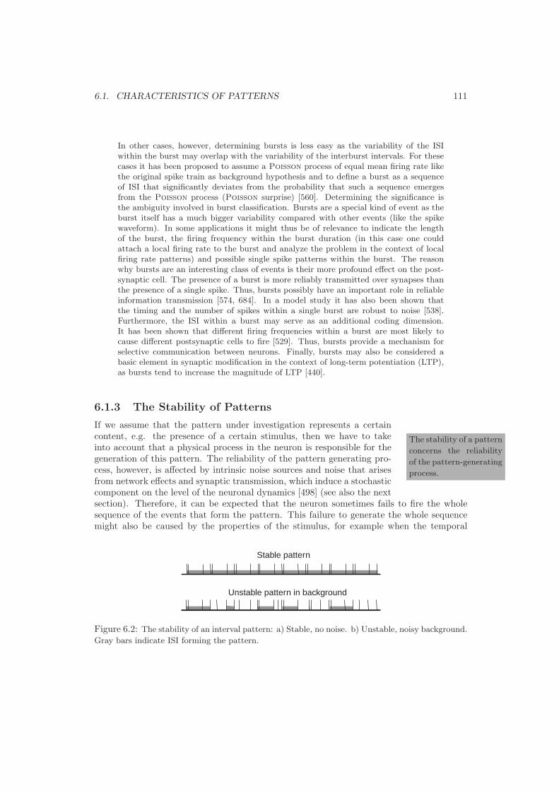
6.1. CHARACTERISTICS OF PATTERNS 111
In other cases, however, determining bursts is less easy as the variability of the ISIwithin the burst may overlap with the variability of the interburst intervals. For thesecases it has been proposed to assume a Poisson process of equal mean firing rate likethe original spike train as background hypothesis and to define a burst as a sequenceof ISI that significantly deviates from the probability that such a sequence emergesfrom the Poisson process (Poisson surprise) [560]. Determining the significance isthe ambiguity involved in burst classification. Bursts are a special kind of event as theburst itself has a much bigger variability compared with other events (like the spikewaveform). In some applications it might thus be of relevance to indicate the lengthof the burst, the firing frequency within the burst duration (in this case one couldattach a local firing rate to the burst and analyze the problem in the context of localfiring rate patterns) and possible single spike patterns within the burst. The reasonwhy bursts are an interesting class of events is their more profound effect on the post-synaptic cell. The presence of a burst is more reliably transmitted over synapses thanthe presence of a single spike. Thus, bursts possibly have an important role in reliableinformation transmission [574, 684]. In a model study it has also been shown thatthe timing and the number of spikes within a single burst are robust to noise [538].Furthermore, the ISI within a burst may serve as an additional coding dimension.It has been shown that different firing frequencies within a burst are most likely tocause different postsynaptic cells to fire [529]. Thus, bursts provide a mechanism forselective communication between neurons. Finally, bursts may also be considered abasic element in synaptic modification in the context of long-term potentiation (LTP),as bursts tend to increase the magnitude of LTP [440].
6.1.3 The Stability of Patterns
The stability of a pattern
concerns the reliability
of the pattern-generating
process.
If we assume that the pattern under investigation represents a certaincontent, e.g. the presence of a certain stimulus, then we have to takeinto account that a physical process in the neuron is responsible for thegeneration of this pattern. The reliability of the pattern generating pro-cess, however, is affected by intrinsic noise sources and noise that arisesfrom network effects and synaptic transmission, which induce a stochasticcomponent on the level of the neuronal dynamics [498] (see also the nextsection). Therefore, it can be expected that the neuron sometimes fails to fire the wholesequence of the events that form the pattern. This failure to generate the whole sequencemight also be caused by the properties of the stimulus, for example when the temporal
Stable pattern
Unstable pattern in background
Figure 6.2: The stability of an interval pattern: a) Stable, no noise. b) Unstable, noisy background.
Gray bars indicate ISI forming the pattern.

112 CHAPTER 6. DEFINING PATTERNS
overlap of stimuli does not allow a neuron to finish the firing of the sequence [444]. Thestability of a pattern concerns the question to what extent a neuron is not able to fire thewhole pattern when confronted with a stimulus that usually generates this pattern [661]. Ifa pattern is unstable in that sense, one expects that not only the sequence of events thatdefines the patterns is present, but also subsequences. The so-called ‘ghost doublets’ [565]that have been detected in single spike trains when looking for interval patterns of length3 are an example of such fragments of sequences. We exemplify the concept of patternstability in Fig. 6.2: The first spike train describes an ideal case, in which the whole spiketrain consists of the repetition of an interval pattern of length 3. The second spike traindescribes the situation, in which the interval pattern and its fragments are immersed in anoisy background. To obtain a formal definition of the stability of a pattern, we restrict ourdiscussion to single train interval patterns where pi,j ≡ 1, ∀i, j and discuss spike trains inthe interval representation. For simplifying notation, we write Xi for Xi,j and define:
Definition 6.10 For interval pattern (X1,∆X1), · · · , (Xl,∆Xl) of length l, the set P l
that contains this sequence and all its subsequences is called pattern group
Pl = (Xi,∆Xi), · · · , (Xi+k,∆Xi+k),
where k = 0, . . . , l − 1 and i = 1, . . . , l − k.
Example 6.1: If the interval pattern is given as 2,3,6,4,8 (we assume ∆Xi ≡ 0 to
simplify notation), then the pattern group is (2),(3),(6),(4),(8),(2,3),(3,6),(6,4),(4,8),
(2,3,6),(3,6,4),(6,4,8), (2,3,6,4),(3,6,4,8),(2,3,6,4,8). If the interval pattern is given as
2,2,2,2,2, then the pattern group is (2),(2,2),(2,2,2),(2,2,2,2),(2,2,2,2,2).
The size of P l depends on the number of equivalent (Xi,∆Xi) in the sequence. If(Xi,∆Xi) = (Xi′ ,∆Xi′) for all i = i′, then P l has l(l+1)
2 elements. If (Xi,∆Xi) =(Xi′ ,∆Xi′) applies for certain i, i′, the set is smaller, depending on the relative positionof the equivalent (Xi,∆Xi) within the sequence. We introduce the following notation:
pi The relative frequency of intervals Xi ± ∆Xi within the data.
N(Xi,∆Xi) The number of appearance of intervals Xi ±∆Xi within the data.
Pl(m) The m-th element of P l
N(Pl(m)) The number of appearance of Pl(m) within the data.
N exp(Pl(m)) The expected number of appearance of Pl(m) within the data.
lPn(m) The length of Pl(m)
Although the expression N exp(Pl(m)) could be approximated analytically, it is for prac-tical applications more appropriate to shuffle the ISI of the spike train and to determine

6.2. THE BACKGROUND OF A PATTERN 113
N exp(Pl(m)) based on the shuffled train. After having determined the number of appear-ances of each sequence of the pattern group for the original and the shuffled train, thepattern stability is defined as follows:
Definition 6.11 For a pattern group P l of an interval pattern, the stability sP of thepattern is
sP =∑
m lPl(m)|N(Pl(m)) − N exp(Pl(m))|2
∑l N((Xi,∆Xi))
,
In this way 0 ≤ sP ≤ 1. If the ISI of a sequence a1, . . . , al only appear within thedata as part of the whole sequence, then sP = 1. Such a pattern is maximally stable. Ifthe sequence and its fragments appear as expected by chance, then sP ≈ 0. There aretwo interpretations of this case: Either one assumes ISI-shuffling as the correct background(see next section) and one concludes that no pattern is present, or one assumes a Poisson
background and concludes the presence of an unstable pattern.
6.2 The Background of a Pattern
6.2.1 The Significance of Patterns
We introduced the term ‘background’ (Def. 6.1) as a statistical concept that describes the‘unpatterned’ firing of a cell. In this way, we implicitly attach a certain ‘meaning’ to thepattern as it may represent a stimulus feature, which is relevant for an animal [671]. Fromthe organism point-of-view, a pattern may serve to predict the presence of a stimulus-feature. This is one way to understand the term ‘significance’. There are, however, twonotions of ‘significance’: First, a pattern can be significant in relation to a backgroundmodel. Establishing this ‘statistical significance’ is a mathematical problem. Second, apattern can be significant in the sense that it allows the establishment of a code relation byrelating patterns with symbols. In this framework, a pattern is significant because it has aninformational content that is important for the behavior of the organism. Describing thisrelation is an empirical problem. Both aspects of significance are, however, interrelated.A wrong background model can lead to the detection of ‘wrong patterns’ which, in laterexperiments, cannot be related to any behavioral significance. In this section, we deal withthe statistical significance of a pattern.
6.2.2 The Poisson Hypothesis
Poisson hypothesis: A
inhomogeneous Poisson
process with refractory
period is a good model
for spike data.
In principle, the probability of an event occurring at any given time coulddepend on the entire history of preceding events. If this is not the caseand the events are statistically independent, then they are the resultof a Poisson process [443, 543, 651, 732] – a popular assumption forneuronal firing (especially for cortical neurons). An important reason forits popularity is its simplicity from a stochastic modelling point of view.In this framework, a spike train is seen as the result of a point process,which is defined as follows:

114 CHAPTER 6. DEFINING PATTERNS
Definition 6.12 Let (t0, tL) be a ordered set of points such that 0 = t0 < t1 < . . . < tL.The series is generated by a Poisson process P(t), t ≥ 0 with rate ρ > 0 if
1. P(0) = 0
2. the random variables P(tk) − P(tk1), k = 1, . . . , L are mutually independent
3. for any 0 ≤ ti < tj and k ∈ N0, P(tj) − P(ti) is a Poisson random variable withprobability distribution
PrP(tj) − P(ti) = k =(ρ(tj − ti))k
k!e−ρ(tj−ti)
If ρ is constant, the Poisson process is called homogeneous. If ρ(t) depends on time,the Poisson process is called inhomogeneous.
The following two statistical measures are important for identifying a Poisson processes:
Definition 6.13 If y = y1, . . . yn is a time series with mean 〈y〉 and variance σ(y), thenthe coefficient of variation cv and the Fano factor F are defined as
cv =
√σ(y)〈y〉 F =
σ(y)〈y〉
If a spike train is given, then the following conditions must be fulfilled in order to claim,that a Poisson process is an appropriate statistical model for the train [432, 543, 692]:
1. The ISI distribution has an exponential decay.
2. For the coefficient of variation of the ISIs cv ∼ 1 holds.
3. For the Fano Factor of the spike count F ∼ 1 holds
4. Consecutive ISIs are statistically independent.
The ISI distribution is usually approximated by the 1D histogram (see section 7.2.1).For calculating cv and F , one has to check the presence of negative correlation on a shorttime scale and positive correlation on a long time scale. Otherwise, when choosing thecounting window unfavorable, one may wrongly conclude that a Poisson process generatedthe spike train [380]. Tests for independence usually rely on the autocorrelation or on testing,whether a Markov-dependency can be found in the data [102, 673]. Such tests are difficultto perform if the firing rate is not stationary [523]. In this case it is difficult to distinguishbetween dependencies that contradict the Poisson hypothesis and non-stationary firingthat still could be modelled by an inhomogeneous Poisson model using an appropriaterate function. A stochastic process is stationary, when its probability distribution doesnot change in time. As the sampling time of a process is always finite, stationarity can,strictly speaking, never be positively established. Only non-stationarity can be detected.Several tests for stationarity have been developed – many of them in the field of economicsand financial markets, where large time series are available. In electrophysiology, however,

6.2. THE BACKGROUND OF A PATTERN 115
it is much more difficult to obtain stationary time series that cover a time interval whichis much longer than the longest characteristic time scale relevant for the evolution of thesystem. As the internal dynamics of the neural system cannot be fully controlled, one has toexpect an increasing non-stationarity the longer the measurement lasts (e.g. due to effects ofadaptation). One way to avoid this problem is to perform different trials and to concatenatethe trains of each trial to one spike train. This new train can, for example, be checked forstationarity using the Kolmogorov-Smirnov test on the distributions obtained for thefirst half of the train and the second half of the train [690]. In general, a practical way fordetecting non-stationarity is to measure the desired property (e.g. the mean ISI) for severalsegments of the data and to check, if they are sufficiently equal.
Is is well-known, that the assumption of independence does not hold for short ISI due tothe absolute and relative refractory period in neuronal firing. The absolute refractory periodis the time interval after occurrence of a spike during which it is not possible to induce a newspike. The relative refractory period is a time interval during which the probability of firinggradually increases to the ‘normal value’. The length of both absolute and relative refractoryperiod depends on the type of neuron (e.g. in retinal ganglion cells both periods are of theorder of several milliseconds [389], whereas in neurons of the corticospinal tract they are ofthe order of one millisecond [622]). Various neuron models based on the Poisson modelcan take these effects into account and, furthermore, include a time-varying rate function.[389, 433, 443]. The Poisson hypothesis claims that a (inhomogeneous) Poisson modelwhich includes refractoriness is a reasonably good description of a significant amount ofspike train data [443, 247]. In the context of our pattern discussion, the hypothesis alsoclaims that the only relevant events that could form patterns are local firing rates. Lookingfor patterns on a finer time scale would not make any sense.
But is the Poisson hypothesis true? The historical analysis demonstrated that thisquestion was already investigated in the sixties to a considerable degree – but a consensus wasnot reached (see section 3.2.3). The majority of the findings indicated that the hypothesisis incorrect. Furthermore, seldom all four conditions that should be fulfilled in order toclaim a Poisson process as an adequate statistical model had been tested. The fourthcondition (Markov dependence) is – in the papers reviewed for this PhD thesis – almostnever mentioned, when the validity of the Poisson hypothesis is claimed. On the otherhand, studies, that looked for this dependence indeed found Markov dependencies up tothe fourth order [209, 230]. Also, most of the newer studies usually use the first three criteriato claim the validity of the Poisson hypothesis. A study of Bair et al., based on the spiketrains of 212 cells in the area MT of macaque monkey, showed that about half of the cells firein accordance to the Poisson hypothesis [377, 378]. This claim was based on the argument,that the distribution of the interspike intervals (and interburst intervals, if the cells wherebursting cells) are of exponential type. A study of Sofky and Koch investigated thismatter using data of 16 cells of V1 (15 non-bursting cells) and 409 neurons of MT (233non-bursting cells) of macaque monkey [685]. As the firing rates were variable, the spiketrains have been split into smaller trains with stationary rates. Those with comparable rateshave been concatenated. By using the coefficient of variation criteria for the concatenatedtrains, it has been concluded that the Poisson hypothesis holds for almost all cells. Similarstudies in the area MT of macaque monkey report a cv even higher than 1 [405, 667].
Although often stated, such positive tests in favor of the Poisson hypothesis, are notincompatible with the existence of patterns in spike train. Only spike trains that fulfill all

116 CHAPTER 6. DEFINING PATTERNS
four criteria of the Poisson hypothesis cannot contain repeating sequences above a certainchance level. This can be easily shown by a simple thought experiment: Assume a spike trainin interval representation generated by a Poisson process. From this spike train, n intervalsthat match the templates (X1 ± ∆X1), (X2 ± ∆X2) and (X3 ± ∆X3) are extracted andarranged to n sequences of the form ((X1,∆X1), (X2,∆X2), (X3,∆X3)). These sequencesthen are randomly reinserted into the train at random positions. The resulting train stillfulfills the criteria 1 to 3 and only misses criterium 4.
6.2.3 Randomization Methods
The Poisson model serves as an important null hypothesis for several pattern detectionmethods. It is, however, not the only possible background. In this section we review themost common null hypotheses (ways of randomization) for pattern detection (see figure 6.3):
1. Uniform randomization: The assumption that every order or timing of events ortime interval between events (latter only over a certain interval) is equally probable.A uniform background is common when looking for order patterns. Examples: [559].
2. Homogenous Poisson randomization: The assumption that the events are Pois-
son distributed. The homogeneous Poisson randomization changes the probabilitydistribution of the original measurement unless the original data were itself Poisson
distributed. Examples: [353, 560, 586, 722].
3. Inhomogeneous Poisson randomization: Like method 2), but taking changes infiring rate into account. This is done by either using a rate function based on knowledgeof the stimulus dynamics (e.g. periodic) or by calculating the firing rate and then byperforming homogeneous Poisson randomization only for events that belong to aninterval with quasi-stationary firing rate. Examples: [353, 722]
4. ISI-shuffling: A common way of randomization for interval patterns: The orderof succeeding intervals is randomly rearranged but the intervals themselves are notchanged. This preserves the 1D ISI histogram. In principle, large changes in firing ratescan be considered by shuffling time segments with quasi-stationary rates separately(inhomogeneous ISI-shuffling). Examples: [444, 725]
5. Spike-jitter randomization: This randomization assumes a jitter ∆T and redis-tributes the timing ti of each spike i within the interval [ti − ∆T, ti + ∆T ] uniformly.Examples: [348, 442].
6. Spike shuffling: This randomization is applied for multi train patterns and allowsto keep the post stimulus time histogram (PSTH) unchanged: For each bin used togenerate the PSTH, the membership of a spike to a train is randomly rearranged.Examples: [562, 639, 725].
7. Spike-count match randomization: This randomization is a more restrictive vari-ant of the spike shuffled background: The shuffling of spikes within a bin across thespike trains is restricted, such that the spike counts of each trial before and after shuf-fling remains comparable, and by forbidding shuffles that would generate ISI shorterthan the empirically derived refractory period. Examples: [379, 627].

6.2. THE BACKGROUND OF A PATTERN 117
before randomization after randomization
uniform
Homogeneous Poisson
Inhomogeneous Poisson
ISI shuffled
firingrate
time
time
spike jittered
spike shuffled
spike count match
time time
time
time
firingrate
time
time
time time
time
∆T: jitter interval
time
time
time
time
time
1
neuronnumber
2
3
4
∆τ
time
time
time
time
1
neuronnumber
2
3
4
time
time
time
time
1
neuronnumber
2
3
4
time
time
time
time
1
neuronnumber
2
3
4
∆τ
∆τ
∆τ
Figure 6.3: Schematic overview of different methods for randomization (see text).
The background models differ in the degree of randomness they impose on the originaldata. This affects the significance of found patterns when compared with the statistical null:In the studies mentioned above, all backgrounds except the last one [379, 627] have led tothe conclusion that patterns have been found. Therefore, when comparing such studies onehas to take into account which way of randomization has been used. Also the use of patterndetection methods should include an assessment of the degree of randomness introduced bythe shuffling procedures (see example 6.2).
Example 6.2: To demonstrate the degree of randomness introduced by the differentshuffling procedures, we use a set of 10 trial spike trains obtained from simple cells
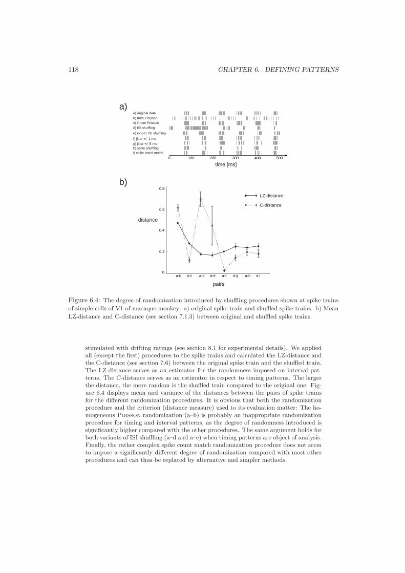
118 CHAPTER 6. DEFINING PATTERNS
100 200 300 400 500
a-c a-e a-g a-i0
0.2
0.4
0
a) original data
b) hom. Poissonc) inhom Poissond) ISI shuffling
e) inhom. ISI shuffling
f) jitter +/- 1 ms
g) jitter +/- 5 msh) spike shufflingi) spike count match
time [ms]
a-b a-d a-f a-h
pairs
distance
0.6
0.8
a)
b)LZ-distance
C-distance
Figure 6.4: The degree of randomization introduced by shuffling procedures shown at spike trains
of simple cells of V1 of macaque monkey: a) original spike train and shuffled spike trains. b) Mean
LZ-distance and C-distance (see section 7.1.3) between original and shuffled spike trains.
stimulated with drifting ratings (see section 8.1 for experimental details). We appliedall (except the first) procedures to the spike trains and calculated the LZ-distance andthe C-distance (see section 7.6) between the original spike train and the shuffled train.The LZ-distance serves as an estimator for the randomness imposed on interval pat-terns. The C-distance serves as an estimator in respect to timing patterns. The largerthe distance, the more random is the shuffled train compared to the original one. Fig-ure 6.4 displays mean and variance of the distances between the pairs of spike trainsfor the different randomization procedures. It is obvious that both the randomizationprocedure and the criterion (distance measure) used to its evaluation matter: The ho-mogeneous Poisson randomization (a–b) is probably an inappropriate randomizationprocedure for timing and interval patterns, as the degree of randomness introduced issignificantly higher compared with the other procedures. The same argument holds forboth variants of ISI shuffling (a–d and a–e) when timing patterns are object of analysis.Finally, the rather complex spike count match randomization procedure does not seemto impose a significantly different degree of randomization compared with most otherprocedures and can thus be replaced by alternative and simpler methods.

6.3. NOISE AND RELIABILITY 119
6.3 Noise and Reliability
6.3.1 What is Noise in Neuronal Systems?
Two views of noise: An
‘unwanted’ component
whose magnitude one
wants to determine. Or:
a component that the
system uses.
From the perspective of the observer of a system, two classes of noise aredistinguished [536]: Measurement noise (or additive noise) refers to thecorruption of observations by errors that are independent of the dynamicsof the system. Measurement noise is a unwanted noise component andone tries to minimize it by optimizing the experimental design and mea-surement instruments, so that no relevant information about the systemis lost. Dynamical Noise, in contrast, is a result of a feedback process bywhich the system is perturbed by a small random amount at each timestep. This noise results due to stochastic elements in signal generation.In spike trains, dynamical noise may affect the probability of spike appearance as well asspike timing. There is, however, a different perspective on the problem of neural noise, asthe distinction between ‘signal’ and ‘noise’ is a distinction usually made from the observer’sperspective. What appears as noise for the observer, may have importance for the neuron.In other words, from the ‘neuron perspective’, the important question is whether noise canhave any functional role for a neuron. This perspective has already been formulated in themid 20th century as we have shown in the historical analysis (see section 3.2.2).
To assess the influence of noise, one distinguishes between internal and external noise. Byinternal noise, we refer to the variability of the spike generating processes (channel gating,ion fluxes etc.) that are attributed to the neuron under investigation. External noise isattributed to the variability of (at least) three aspects: First, the (possible) noisy characterof the input which emerges from the activity of all neurons projecting to the neuron underinvestigation. Second, the activity of glia cells that are known to influence neuronal firing[476]. Third, fluctuations in the extracellular chemical environment of the neuron underinvestigation. The influence of these external noise sources is difficult to measure. Especiallythe second and third aspect are seldom investigated, whereas the first aspect is analyzedunter the general notion of ‘background activity’ (see below). It is an open question whetherinternal or external noise sources have a ‘purely’ random basis (i.e. referring to quantumeffects) or express a higher-dimensional deterministic part of the dynamics. One can suspectthat especially external noise sources are of the latter case [642, 730].
6.3.2 Noise Sources in Neurons
In the historical part we have demonstrated that the ‘noisiness’ of neurons became a con-troversial topic as soon as the information vocabulary was applied in neuroscience. Later,several neuronal sources of noise have been investigated. The underlying goal of these in-vestigations is to estimate to what extent these noise sources change the timing of spikes,suppress spikes that ‘should’ occur due to the stimulus characteristics or generate sponta-neous spikes. Today, a rather complete picture of neuronal noise sources is available (seeFig. 6.5). We list these sources according to the pathway of incoming signals and concentrateour discussion on cortical neurons:
1. Background activity: Background activity is a component of noise in cortical neu-rons for in vivo conditions. Although also glia cell activity and fluctuations in the
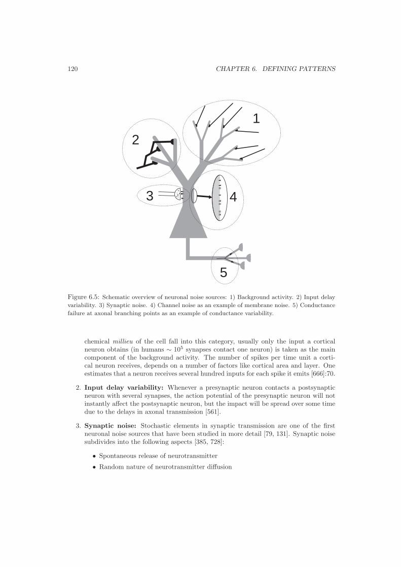
120 CHAPTER 6. DEFINING PATTERNS
1
2
3 4
5
Figure 6.5: Schematic overview of neuronal noise sources: 1) Background activity. 2) Input delay
variability. 3) Synaptic noise. 4) Channel noise as an example of membrane noise. 5) Conductance
failure at axonal branching points as an example of conductance variability.
chemical millieu of the cell fall into this category, usually only the input a corticalneuron obtains (in humans ∼ 105 synapses contact one neuron) is taken as the maincomponent of the background activity. The number of spikes per time unit a corti-cal neuron receives, depends on a number of factors like cortical area and layer. Oneestimates that a neuron receives several hundred inputs for each spike it emits [666]:70.
2. Input delay variability: Whenever a presynaptic neuron contacts a postsynapticneuron with several synapses, the action potential of the presynaptic neuron will notinstantly affect the postsynaptic neuron, but the impact will be spread over some timedue to the delays in axonal transmission [561].
3. Synaptic noise: Stochastic elements in synaptic transmission are one of the firstneuronal noise sources that have been studied in more detail [79, 131]. Synaptic noisesubdivides into the following aspects [385, 728]:
• Spontaneous release of neurotransmitter
• Random nature of neurotransmitter diffusion

6.3. NOISE AND RELIABILITY 121
• Chemical reactions in the synaptic cleft
• Varying number of released vesicles during stimulation
• Varying size of released vesicles.
• Varying number of postsynaptic receptors activated by transmitter release
4. Membrane noise: Membrane noise is a collective term for several aspects that af-fect the cell membrane. The most important component is called channel noise, therandomly opening and closing of (usually voltage gated) ion channels [71, 755]. Aminor noise source in membranes, called Johnson noise, is caused by thermal effects.Certainly, also small lesions in the membrane are a noise source.
5. Conductance variability: The current flow within the neuron as well as axonalaction potential spread may be affected by the internal cellular structure (cytoskeletonetc.). This aspect has been, however, rarely investigated (we found no reference on thismatter). One aspect of conductance variability is caused by axonal branching points,as sometimes the action potential does not reach some of the synaptic terminals of theaxon and is unable to induce a reaction at the postsynaptic site [417].
Experiments to investigate the significance of each noise source are not easy to conduct.It is obvious that there is a large difference between the in vitro and the in vivo condi-tion, as in latter case the background activity will play a major role [523]. Usually, theterm ‘spontaneous activity’ is used when referring to the spiking activity of a single neurondriven by background noise [603]. The role of the background noise for the variability ofneuronal firing will be discussed in the next section. Concerning the other noise sources,estimations have been conducted in empirical as well as model studies using detailed neuronsimulations. Already one of the first (empirical) studies on this issue (1968) concluded thatsynaptic noise mainly accounts for the observed firing variability [64]. A model study whichinvestigated the magnitudes of the voltage standard deviations of thermal noise, channelnoise and synaptic noise in a space-clamped somatic membrane patch confirmed this finding[591]: Thermal noise and Na+ channel noise were one magnitude lower (2 × 10⁻² mV and6×10−2 mV) compared to K+ channel noise and synaptic noise (5×10⁻¹ mV and 9×10⁻¹
mV). Which aspect of synaptic noise is the most relevant? This question has, for example,been analyzed in hippocampal neurons. Four potential causes for synaptic unreliability havebeen investigated: Threshold fluctuations at the postsynaptic site, conduction failures at thepresynaptic site, temperature, and probabilistic transmitter release. The study concludedthat the probabilistic release mechanisms at low capacity synapses are the main cause ofunreliability of synaptic transmission [361].
The dominant role of synaptic noise does not mean that membrane noise is unable toinduce spontaneous spikes or a failure of firing a spike. Several model studies suggest, that‘additional’ or ‘missing’ spikes also can occur due to membrane noise [424, 659, 755, 756].This is so because what matters is not the total number of ion channels – this number ishigh and fluctuations would usually have been averaged out – but the number of channelsthat are open near threshold – which is considerably smaller. Moreover, the membranepatches involved in spike generation or transmission, such as nodes of Ranvier, also containonly small numbers of channels, so that fluctuations in channel gating cause fluctuations infiring. Counteracting channel noise needs an increase in the number of ion channels. This

122 CHAPTER 6. DEFINING PATTERNS
implies a large energetic investment for the cell, not only because of the costs of creatingthe channel but also because large ionic currents imply a greater accumulation of ions andthus increase the demand of ion pumps. As the energetic costs per action potential areconsiderable,3 channel noise is probably the result of a trade-off between the energetic costsassigned with higher channel numbers and the reliability of firing. The role of input delayvariability has been investigated in experimental as well as in model studies [410, 597].These studies concluded that the standard deviation of the output jitter in spike timing islinearly related to the standard deviation of the input jitter with a constant smaller thanone. Furthermore, anatomical studies (reviewed in [561]) suggest a interbouton-distance ofaround 15 µm, implying a delay of only a few µs. Therefore, input delay variability hasprobably no decisive role as a noise source.
6.3.3 The Reliability of Neurons
Reliability (variability)
concerns the ability of
neurons to react similar
to similar inputs.
The historical analysis demonstrated that neuronal ‘(un)reliability’ hasbeen analyzed as soon as an experimental setup that provided stablemeasurements of spikes were available (1930s, see section 2.3.3). It laterbecame an important issue when the question emerged how a reliable sys-tem behavior could emerge out of unreliable elements (see section 3.2.5).In other words, if we discuss the reliability (or variability) of neuronalfiring, we are judging the performance of the neuron from an observer-
point-of-view. The basic idea is to expose a neuron to identical stimulus conditions and tosee, whether identical responses result. Sometimes, the term ‘variability’ of firing is usedto classify single spike trains in the sense that ‘variable’ trains are Poisson trains (e.g. in[523]). We, however, suggest not to use the terms ‘variability’ or ‘reliability’ for this type ofproblem (i.e. the question, what degree of randomness a spike train has). These conceptsshould refer to the problem, whether a neuron is able to maintain a certain firing behaviorin different trials. For this problem, different measures of reliability have been proposed:
1. The simplest measure or reliability is the spike count in a certain time window,respectively the Fano factor of the spike count [277] (alternatively, the coefficient ofvariation of the spike count is used as a measure of variability).
2. Another possible measure is to evaluate, if a certain firing rate pattern is preserved.The simplest such pattern is to compare the peak firing rates [654].
3. A common measure refers to the reliable spike timing of some particular spikes, whichis usually measured based on the post stimulus time histogram (PSTH). This measureneeds a criterion to identify the ‘important spikes’ whose reliable preservation of spiketiming is considered as relevant. Usually, this is done by smoothing the PSTH by somefilter function and to define a threshold value to determine the important spikes. Thereliability is then measured as the fraction of spikes that lie in the ‘important peaks’
3In a study on photo-receptors and interneurons in the fly compound eye [553], the energy consumptions interms of ATP molecules has been determined. It has been estimated, that the cell needs 104 ATP moleculesto transmit a bit in a chemical synapse and 106 − 107 ATP molecules for graded signals in an interneuronor a photoreceptor. These numbers are five to eight orders of magnitude higher than the thermodynamicminimum required for these operations.

6.3. NOISE AND RELIABILITY 123
of the PSTH and the precision is defined as the mean standard deviation of the spiketimings for all spikes that are part of these ‘important peaks’ [588] (a similar approachwhere the spikes of different trials are projected to one train has been proposed in[725]). An alternative measure only concerns the timing of the first spike (reliabilityof response latency) [616]. If the spike timing of all spikes is considered, distancemeasures are applied (see section 7.6).
4. Finally, the reliable presence of certain interval patterns could serve as a measurefor reliability. In this respect, distance measures that take the temporal order of spikesinto account could serve as a measure. We will present this approach in more detailin section 7.6. (a comparable approach is the use of the entropy of spike trains [453]).
Either coding or compu-
tation can be called ‘reli-
able’.
These measures of reliability fall into the context of the neural cod-ing discussion: Can a neuron maintain a certain encoding of (sensory)information? This addresses the general problem whether a neuron isable to transmit information reliably. An alternative concept of reliabil-ity refers to neural computation. Here, the question is: Can a neuronalways perform the same computation when the set of inputs the neuronis confronted with corresponds to the same type of computation? To test this variant ofreliability, one has to find a set of different inputs that nevertheless leads to the same output(in one of the four meanings above). To analyze to what extent a certain input affects thereliability of computation, the following test procedure has been proposed [442]: Choose atime interval, bin the time axis using this interval and jitter the spikes within the borders ofeach bin. As long as the choice of the partitioning interval does not change the reliability ofthe output of the system, one is within the class of inputs that generates the same output.Note that reliability in this context also can mean that a neuron always generates a randomoutput for a large class of inputs. Such a neuron could be considered as a ‘reliable noisegenerator’. In other words, the concept of reliability is dependent on the context one isinterested in – neural coding or neural computation. The determination of the reliability ofneurons in experiments has to consider several practical problems:
1. One will expect a difference in reliability under in vitro or in vivo conditions. It isgenerally assumed that this difference results from the higher background activity, andis not due to changes in internal noise sources in the neuron [523].
2. The design of the experiment is also important. Measuring the reliability of responsefor directly injected current inputs will lead to different results than measuring the reli-ability for stimuli the neuron receives via the sensory pathway. There is the possibilitythat variability emerges due to overlooked sources of variability in the experimentaldesign. For example, a study showed that eye movements cause a large component ofresponse variance in alert monkeys [515]. It is thus crucial that eye position duringdata collection is carefully monitored, when doing such studies in the visual system.Besides, one has also to take into account the firing rates one obtains, as for high firingrates, spike timing reliability could be a result of the refractory period of neurons [389].
3. The kind of stimulus used will have an impact on the result of reliability estimations.First, the stronger the stimulus the more reliable the neuron reacts (for example strong
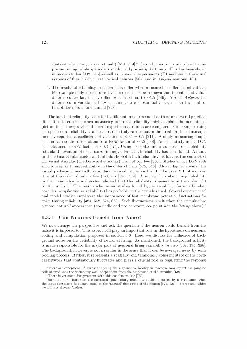
124 CHAPTER 6. DEFINING PATTERNS
contrast when using visual stimuli) [644, 749].4 Second, constant stimuli lead to im-precise timing, while aperiodic stimuli yield precise spike timing. This has been shownin model studies [402, 516] as well as in several experiments (H1 neurons in the visualsystems of flies [453]5, in rat cortical neurons [588] and in Aplysia neurons [48]).
4. The results of reliability measurements differ when measured in different individuals.For example in fly motion-sensitive neurons it has been shown that the inter-individualdifferences are large, they differ by a factor up to ∼3.5 [749]. Also in Aplysia, thedifferences in variability between animals are substantially larger than the trial-to-trial differences in one animal [758].
The fact that reliability can refer to different measures and that there are several practicaldifficulties to consider when measuring neuronal reliability might explain the nonuniformpicture that emerges when different experimental results are compared. For example, usingthe spike count reliability as a measure, one study carried out in the striate cortex of macaquemonkey reported a coefficient of variation of 0.35 ± 0.2 [211]. A study measuring simplecells in cat striate cortex obtained a Fano factor of ∼1.2 [448]. Another study in cat LGNcells obtained a Fano factor of ∼0.3 [575]. Using the spike timing as measure of reliability(standard deviation of mean spike timing), often a high reliability has been found: A studyin the retina of salamander and rabbits showed a high reliability, as long as the contrast ofthe visual stimulus (checkerboard stimulus) was not too low [390]. Studies in cat LGN cellsshowed a spike timing reliability in the order of 1 ms [575, 645]. Also in higher areas of thevisual pathway a markedly reproducible reliability is visible: In the area MT of monkey,it is of the order of only a few (∼3) ms [376, 409]. A review for spike timing reliabilityin the mammalian visual system showed that the reliability is generally in the order of 1to 10 ms [375]. The reason why newer studies found higher reliability (especially whenconsidering spike timing reliability) lies probably in the stimulus used. Several experimentaland model studies emphasize the importance of fast membrane potential fluctuations forspike timing reliability [384, 548, 624, 662]. Such fluctuations result when the stimulus hasa more ‘natural’ appearance (aperiodic and not constant, see point 3 in the listing above).6
6.3.4 Can Neurons Benefit from Noise?
We now change the perspective and ask the question if the neuron could benefit from thenoise it is imposed to. This aspect will play an important role in the hypothesis on neuronalcoding and computation proposed in section 6.6. Here, we discuss the influence of back-ground noise on the reliability of neuronal firing. As mentioned, the background activityis made responsible for the major part of neuronal firing variability in vivo [369, 374, 388].The background, however, is not irregular in the sense that it can be averaged away by somepooling process. Rather, it represents a spatially and temporally coherent state of the corti-cal network that continuously fluctuates and plays a crucial role in regulating the response
4There are exceptions: A study analyzing the response variability in macaque monkey retinal ganglioncells showed that the variability was independent from the amplitude of the stimulus [438].
5There is yet some disagreement with this conclusion, see [750].6Some authors claim that the increased spike timing reliability could be caused by a ‘resonance’ when
the input contains a frequency equal to the ‘natural’ firing rate of the neuron [525, 526] – a proposal, whichwe will not discuss further.

6.4. FUNCTIONAL ASPECTS OF SPIKE PATTERNS 125
strength of cortical neurons to sensory inputs [373, 422, 479]. Furthermore, model studiessuggest that background noise might also enhance the precision of spike timing [763]. Severalother studies showed that the background noise a neuron receives correlates with stimulusproperties and is thus potentially an additional information source for the neuron [745, 749].Finally, background noise may have furthermore supportive functions in sensory systemsfor several specific purposes (enhancement of contrast invariance of orientation tuning [365],improved encoding of the stimulus waveform in the auditory system [569]). Such findingshave been recently connected to a concept developed in physics: stochastic resonance.
Stochastic Resonance: The phenomenon of stochastic resonance has been found innoise driven, periodically modulated bistable systems. When the intensity of the ex-ternal noise is properly tuned to the internal parameters of the bistable system, thenthe external noise and the periodic driving mechanism interact by pumping power fromthe whole noise spectrum into a single mode which is coherent with the signal. Thisproduces a well defined peak in the power spectrum of the output signal and the corre-sponding signal to noise ratio has a maximum. For larger noise amplitudes the signalis increasingly corrupted. In the past years, this concept of stochastic resonance hasgained much attention in biology. Several authors suppose that stochastic resonanceplays an important role in the nervous system [728, 754]. This speculation is supportedby physiological experiments and model studies: The phenomenon of stochastic reso-nance has for example been demonstrated for voltage-dependent ion channels [391] andcrayfish mechanoreceptors [463]. Model studies showed the phenomenon of stochasticresonance in pattern detection experiments using holographic neurons [702] or in ex-periments using the FitzHugh-Nagumo model [589]. They show how neurons may usenoise in order to enhance their sensitivity to detect external stimuli. One model studygave more insight into the detailed process of stochastic resonance on the level of themembrane. In a model study with Hodgkin-Huxley-type neurons, the influence ofnoise on the detection and timing precision of neural signals has been investigated. Ithas been shown, that the timing precision is improved by internal noise sources only fordeterministically subthreshold stimuli [634]. In a detailed model of a morphologicallyreconstructed neocortical pyramidal neuron, it furthermore has been shown, that theintroduction of voltage fluctuations increased responsiveness. This again is consideredas a possible example of stochastic resonance [522].
6.4 Functional Aspects of Spike Patterns
In this section, we discuss some main theoretical frameworks, which may explain the presenceand functional role of patterns. Early investigations (1960s) distinguished two causes fortemporal patterns found in neuronal spike trains: Either neurons follow patterned time cuesof stimuli, or patterns result from intrinsic timing cues (e.g. pacemaker cells) [54]. Thisbasic distinction that either aspects inherent to neurons (like refractoriness) or aspects ofthe stimulus cause the presence of patterns, is still made [400]. It, however, disregards therole of the neuronal network in which the neuron is embedded as a specific connectivity mayfavor certain types of patterns and exclude others [704]. Thus, patterns may result fromthree general causes: The temporal structure of the stimulus, the biophysical properties ofneurons, or the network connectivity. This classification of potential causes does not implya functional classification. For example, stimulus aspects may cause patterns which are
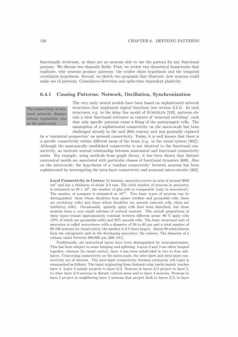
126 CHAPTER 6. DEFINING PATTERNS
functionally irrelevant, as there are no neurons able to use the pattern for any functionalpurpose. We discuss two thematic fields: First, we review two theoretical frameworks thatexplicate, why neurons produce patterns: the synfire chain hypothesis and the temporalcorrelation hypothesis. Second, we sketch two proposals that illustrate, how neurons couldmake use of patterns: Coincidence-detection and spike-time dependent plasticity.
6.4.1 Causing Patterns: Network, Oscillation, Synchronization
The connectivity of neu-
ronal networks displays
certain regularities also
on the micro-scale.
The very early neural models have been based on sophisticated networkstructures that implement logical functions (see section 3.2.4). In suchstructures, e.g. in the delay line model of Strehler [243], patterns ob-tain a clear functional relevance as causers of ‘neuronal switching’, suchthat only specific patterns cause a firing of the postsynaptic cells. Theassumption of a sophisticated connectivity on the micro-scale has beenchallenged already in the mid 20th century and was gradually replaced
by a ‘statistical perspective’ on network connectivity. Today, it is well known that there isa specific connectivity within different areas of the brain (e.g. in the visual system [362]).Although the anatomically established connectivity is not identical to the functional con-nectivity, an intricate mutual relationship between anatomical and functional connectivityexists. For example, using methods from graph theory, it has been shown that distinctanatomical motifs are associated with particular classes of functional dynamics [688]. Alsoon the micro-scale, the hypothesis of a ‘random connectivity’ between neurons has beensophisticated by investigating the intra-layer connectivity and neuronal micro-circuits [462].
Local Connectivity in Cortex: In humans, neocortex covers an area of around 2600cm2 and has a thickness of about 2-4 mm, The total number of neurons in neocortexis estimated as 28 × 109, the number of glia cells is comparable (only in neocortex!).The number of synapses is estimated as 1012. Two basic types of neurons can bedistinguished: those whose dendrites bear spines (stellate and pyramidal cells, theseare excitatory cells) and those whose dendrites are smooth (smooth cells, these areinhibitory cells). Occasionally, sparsely spiny cells have been described, but theseneurons form a very small subclass of cortical neurons. The overall proportions ofthese types remain approximately constant between different areas: 80 % spiny cells(70% of which are pyramidal cells) and 20% smooth cells. The basic structural unit ofneocortex is called minicolumn with a diameter of 50 to 60 µm and a total number of80-100 neurons (in visual cortex, the number is 2.5 times larger). About 80 minicolumnsform the ontogenetic unit in the developing neocortex: the column. The diameter of acolumn varies between 300-600 µm [460, 611].
Traditionally, six neocortical layers have been distinguished by neuroanatomists.This has been subject to some lumping and splitting: Layers 2 and 3 are often lumpedtogether, whereas (in visual cortex), layer 4 has been subdivided in two to four sub-layers. Concerning connectivity on the micro-scale, the inter-layer and intra-layer con-nectivity are of interest. The inter-layer connectivity between excitatory cell types issummarized as follows: The input originating from thalamic relay nuclei mainly reacheslayer 4. Layer 4 mainly projects to layer 2/3. Neurons in layers 2/3 project to layer 5,to other layer 2/3 neurons in distant cortical areas and to layer 4 neurons. Neurons inlayer 5 project to neighboring layer 5 neurons that project back to layers 2/3, to layer

6.4. FUNCTIONAL ASPECTS OF SPIKE PATTERNS 127
6 neurons, that project back to the thalamus and to layer 4, and finally to subcorticalareas. Layer 5 is thus expected to be the main output area [416, 459, 636, 719].
Furthermore, there is a specific intra-layer-connectivity, which has been extensivelyanalyzed, e.g. in the barrel cortex of rats. The most information is available for layers4, 5 and 2/3. In layer 4 (rat barrel cortex), around 70 % of the excitatory cell are spinystellate cells and 15 % are pyramidal cells. These cells are highly connected withina single barrel: 91% of the axons and 97% of the dendrites of neurons remain withinthe home barrel, and also the analysis of functional connections showed, that synaptictransmission appears to be restricted to a single barrel. This motivates the claim that abarrel acts as a single processing unit. Pairwise testing of neurons with distances below200 µm show, that one fifth of the pairs were directly connected. The probability ofconnectivity of a single excitatory neuron in a barrel is estimated in the order of 0.31-0.36. It is furthermore claimed, that L4 excitatory neurons mediate a reliable and strongfeed-forward excitation of thalamic signals within L4 and to L2/3, so that layer 4 actsas an amplifier of thalamo-cortical signals. [475, 474, 580, 636]. The layers 2/3 receivetheir input mainly from layer 4. The (functional) connectivity of the pyramidal cells hasbeen estimated as 0.09. More than 70 % of all synapses on a layer 2/3 pyramidal celloriginate from other pyramidal cells within a radius of 600 µm [519, 619, 691]. Layer5 is the major cortical output layer. The two major layer 5 pyramidal cell subtypesare intrinsically burst spiking and regular spiking. It has been estimated that eachpyramidal neuron is connected to at least 10% of the neighboring pyramidal cells by fastexcitatory glutamate synapses. It has been proposed, that (tufted) layer 5 pyramidalneurons form local networks of around 300 µm diameter consisting of a few hundredneurons, which are extensively interconnected with reciprocal feedback. Statisticalanalysis of the synaptic innervation suggest that the network is not randomly arranged,the degree of specificity of synaptic connections seems to be high [474, 594, 595, 664].
There is an ongoing debate, how precisely the connectivity pattern within a micro-circuitreplicates [689] and to what extent neocortical micro-circuits discovered in primary sensoryareas generalize to the whole cortex [459]. Furthermore, it is not clear, how fast the networkconnectivity can change, e.g. due to learning. Recent studies showed rather discrepantresults [631]: Two studies in mice revealed different surviving times of spines. In one study[727], even the stablest pool (60% of spines) had a limited lifetime of about 100 days (barrelcortex), whereas in a second study [512], about 96% of spines remained stable for over amonth, translating to a half-life of more than 13 months. This implies that synapses couldpersist throughout a mouse’s lifetime (visual cortex). It furthermore remains open if thetime-scale of changes on the anatomical level is the same as the time scale of changes onthe functional level. The question whether the structure of a specific micro-circuit prohibitscertain spike patterns is probably hard to answer. Model studies suggest, that already thepositioning of a single synapse along the distal-proximal axes may matter. Earlier studiesclaimed that the size of the individual somatic EPSP is independent of the dendritic inputlocation [585, 584]. More recent model studies, however, argue that this independence isonly valid for the in vitro case and that in vivo, distal synapses become weaker than proximalsynapses [579]. This results from a several-fold increase in dendritic membrane conductancedue to the activity of many synapses in vivo. They concluded that the dendritic location(proximal versus distal) of even a single excitatory synapse activated in the presence ofmassive background synaptic bombardment can have a noticeable effect on axonal spikeoutput (shifting or disappearing of spikes) [577].

128 CHAPTER 6. DEFINING PATTERNS
The synfire hypothesis
may explain information
transmission, but not in-
formation processing.
Due to the difficult questions that emerge when the micro-structureof the neuronal network is related to the occurrence of specific temporalpatterns, statistical approaches are used. They assume a locally randomconnectivity based on a certain probability of connectivity, but requiresome ordered connectivity pattern on the level of groups of neurons. Afamous hypothesis of this type is the synfire hypothesis.7 The focus of the
synfire hypothesis is the transmission of information by putting emphasis on synchronousfiring events, but it doesnot provide a scheme of how this information is processed.
The Synfire Hypothesis: The synfire hypothesis claims the existence of networksof groups of cells with converging connections between these groups (synfire chains)[350, 352, 358]. Each link in a synfire chain consists of a set of synchronously firingneurons. Each set excites synchronous firing in the next set, which in turn excite thenext set of neurons synchronously etc. The prerequisites of the hypothesis are: 1)The cells in the sending node are indeed firing synchronously. 2) The synapses mustbe strong enough to ensure synchronous firing of the cells in the receiving node. 3)A mechanism exists that prevents an accumulation of a small jitter in firing times ofthe synchronous volleys. Synfire chains imply the existence of multi train patterns ofsingle spikes that stretch over time intervals of up to hundreds of milliseconds. Severalclaims about the existence of such patterns have been made (see section 6.5). Some ofthese studies explicitly tested whether the detected multi train patterns are consistentwith the synfire chain hypothesis. In one study, two alternatives have been investigated[639]: Either the patterns are the result of slow dendritic processes [381] or they emergeas the result of superposition of periods of regular firing across different neurons. Thefirst alternative has been considered as unlikely, as it is hard to imagine that a neuronis able to ‘remember’ a given spike for a delay of hundreds of milliseconds and to fire asecond, precisely (± 1 ms) timed spike, while (between these two spikes) the same cellfires other spikes. The second alternative leads to the expectation, that mostly singlespike patterns should be detected, which was not the case in the study. Furthermore,there was no excess of intervals in the range of 15-100 ms: the corresponding periodsof the observed in vitro oscillations, making it unlikely that such oscillations werepresent. The authors concluded that the patterns found are best explained by thesynfire hypothesis. A second, in vitro study in rat V1 investigated spontaneous firingand found synchronous spikes correlated among networks of layer 5 pyramidal cells[592]. These networks consisted in 4 or more cells. Sets of neurons are also sequentiallyactivated several times. These findings are compatible with the synfire hypothesis. Ina further study in cat LGN it has been shown that neighboring geniculate neuronswith overlapping receptive fields of the same type (on-center or off-center) often firespikes, that are synchronized within 1 ms [363]. They project to a common corticaltarget, where synchronous spikes are more effective in evoking a postsynaptic response,which is again compatible with the synfire chain model. Finally, the plausibility ofthe synfire hypothesis has been tested in several model studies. One study came tothe conclusion, that a near-synchronous wave of activity can propagate stably alonga synfire chain [520]. A second model demonstrated how a synfire chain of excitatoryneurons in combination with two globally inhibitory interneurons that provide delayedfeed-forward and fast feedback inhibition recognizes order patterns (a certain sequenceof neurons that fired) [530].
7In 1953, George H. Bishop and Margaret Chalre proposed a model of propagation of neuronalexcitation that may be called a forerunner of the synfire model of Abeles, see [34]: Figure 3.

6.4. FUNCTIONAL ASPECTS OF SPIKE PATTERNS 129
Generally, synchronization as well as oscillations in neuronal firing are phenomena, thatare considered important for temporal representation and long-term consolidation of infor-mation in the brain (see [413] for a recent review). First, we briefly discuss oscillations.Oscillations express themselves via periodically appearing interval patterns in single spiketrains. For the general case, we can define oscillations as follows
Definition 6.14 A single spike train which is described as the repetition of a interval pat-tern (p1,j ,X1,j ,∆X1,j), · · · , (pl,j ,Xl,j ,∆Xl,j) of length l is said to reflect an oscillation ofperiodicity l.
A more detailed introduction into oscillations within the framework of dynamical sys-tems theory is provided in section 6.6.1. It is well-known that several types of neuronsare capable to generate intrinsic oscillations [576]. Oscillations appear in several functionalunits of the nervous system: the olfactory system, the visual system, the hippocampus andin the somatosensory and motor cortices [507] (some further examples will be provided insection 6.5). Their functional role is usually associated with the possibility that oscillationsmay serve as a timing framework necessary for ensembles of neurons to perform specificfunctions [414, 478, 717]. A study in rat cortex for example demonstrated, that oscilla-tions induce sinusoidal subthreshold oscillations, and thus periodically recurring phases ofenhanced excitability of the neuron [746]. Weak and short-lasting EPSP evoke dischargesonly if hey are coincident within a few milliseconds with these active membrane responses.Thus, oscillations seem to impose a precise temporal window for the integration of synapticinputs, favoring coincident detection. But the detection of oscillations does not imply perse that they have a function. One example, where oscillations are probably not functionallyrelevant, are oscillatory patterns in the visual system due to the phase locking of neuronalresponses to the refresh rate of computer display monitors, on which visual stimuli are dis-played. Such oscillations are a well-known artefact in visual experiments [483]. In the catvisual system, for example, it has been shown that almost all LGN cells and substantialfractions of simple and complex cells are sensible for a refresh rate of 60 Hz [757]. It is alsoknown that retinal and LGN neurons of cats can lock to the flicker frequencies from fluores-cent tubes (100 Hz), which result of the 50 Hz alternating current current [472]. Anotherstudy in V1 of macaque monkey demonstrated that more than 50% of all measured neuronssynchronized to the refresh rate of 60 Hz [604]. This type of oscillations, however, does notseem to have perceptual consequences [734]8 – but this temporal artefact has a significantinfluence when analyzing single and multi train patterns in the visual system, especiallywhen cross-correlation techniques are used [757].
Synchronization is always a multi train phenomenon and shows up as a successionof unitary events. The basic problem when claiming the occurrence of synchronization isthe same as in pattern detection in general: One has to determine a time interval withinwhich spikes are called ‘synchronous’ [734] and one has to compare the empirically derivednumber of unitary events with the number obtained after a certain type of randomization[503]. Synchronized oscillations show up as unitary events of a certain periodicity andare thus a higher order pattern. Alike oscillations, synchronization in neuronal firing has
8One the other hand, these findings may be a neurophysiological basis for the discomfort reported by indi-viduals working in environments illuminated by fluorescent tubes or for more severe effects like photosensitiveepilepsy, headaches and eyestrain [537, 581].

130 CHAPTER 6. DEFINING PATTERNS
been found in the visual system (retina, LGN, V1 [734]), the olfactory system – where (asshown in bees) the blocking of synchronization impairs the discrimination of molecularlysimilar odors [713] and (as shown in locust) neurons capable to read out the synchronizedoscillatory firing of groups have been found [582] – and the motor system, where (as shownin macaque monkey) synchronization (∆Xi,j = 5 ms) is associated with distinct phasesin the planning and execution of voluntary movements [650]. Basically two possibilitiesconcerning the functional role of synchronization are discusses: It might allow a reliableinformation transfer and offers an additional coding dimension for increased informationtransfer. The first possibility is discussed within the synfire chain model so that we focushere only the second aspect. Generally, as neuronal responses may synchronize without arise in neuronal firing rate, an additional coding dimension is provided [452]. In vision,this might solve the ‘bottleneck problem’: As the number of possible patterns of unitaryevents largely exceeds the number of ganglion cells, this might allow the retina to compressa large number of distinct visual messages into a small number of optic nerve fibers [606].Experimental studies have shown that (in salamander retina) nearby neurons fire up to20-fold more often synchronously than expected, given the fact that they share the sameinput ([607], ∆Xi,j = 20 ms) and that (in cat LGN) considerably more information canbe extracted from two cells if temporal correlations between them are considered [441] (theaverage increase is 20 % for strongly correlated pairs of neurons). The additional codingdimension is also expressed by the idea that transiently synchronized groups of neuronsreflect a read-out of a certain spike pattern. A model study demonstrated, that the patternof synaptic connections can be set such that synchronization within a group of neuronsoccurs only for selected spatiotemporal spike patterns [524]. However, also synchronizationcan appear without having any functional role. For example, synchronization may emergeas a mere coincidence when measuring two pacemaker neurons or may result from a commoninput source [179, 734]. Difficulties may also arise with the classical test used for detectingsynchrony, the cross-correlogram. Based on this test, a peak at zero time is taken as evidencefor synchronous firing of two neurons. This condition, however, is not sufficient. A studyusing model LGN neurons demonstrated that also in the absence of any synaptic or spikesynchronizing interaction between two geniculate neurons, slow covariations in their restingpotentials can generate a cross-correlogram with a center peak. This can erroneously betaken as evidence for a fast spike timing synchronization [407].
The Temporal Correlation Hypothesis: A theoretical framework where both oscil-lations and synchronization gain a functional interpretation is the temporal correlationhypothesis. The hypothesis addresses the following problem: If an assembly of neuronscodes for a single perceptual object then a mechanism should bind the different sensorialmodalities of the object together (‘binding problem’). The basic idea (first proposed1974 [161]) is that the discharges of neurons undergo a temporal patterning and be-come synchronized if they participate in the encoding of related information [747]. Thefollowing predictions derive from this hypothesis [677]: 1) Spatially segregated neuronsshould exhibit synchronized response periods if they are activated by stimuli that aregrouped into a single perceptual object. 2) Individual cells should be able to rapidlychange the partners of synchronous firing, if stimulus configurations change and requirenew associations. 3) If more than one object is present, several assemblies separatedby different synchronization patterns should emerge. Several studies claimed to havefound support for these predictions: In the primary visual cortex (cat, monkey), neu-

6.4. FUNCTIONAL ASPECTS OF SPIKE PATTERNS 131
ronal oscillations in the gamma frequency band (40-60 Hz) have been found that occurin synchrony from spatially separated neurons (same column, across columns, and be-tween the two hemispheres), that the synchronization is influenced by global stimulusproperties, and that set of cells with overlapping but differently tuned receptive fieldssplit into two independently synchronized assemblies [465, 470, 471, 508]. These andother findings (reviewed in [469, 505, 637, 678, 679]) made the temporal correlationhypothesis a widely debated proposal.
Severe critique was raised against the temporal correlation hypothesis. It appeareddifficult to replicate the results reported by the Singer and Eckhorn group. Eitheroscillations were not found or, if they were, they appeared to be rhythmic responsesnot correlated to the stimulus [759, 484, 726], but rather resulting from spontaneousoscillations of a subpopulation of retinal ganglion cells [501]. Recently, a careful experi-mental study in area MT that tested whether neuronal synchrony constitutes a generalmechanism of visual feature binding did not find evidence for the temporal correlationhypothesis [632]. Furthermore it has been criticized that the time necessary to establishan oscillatory group (tenths of milliseconds) is not compatible with the fast reactiontimes observed [726] (this critique has later been rejected, see [679]) and that oscilla-tions, which are not a response to a visual feature, will seriously disrupt the system, ifoscillatory activity is important for the establishment of synchrony [503]. In a detailedcritical review in 1999, the temporal correlation hypothesis has been classified as in-complete because it describes the signature of binding without detailing how bindingis computed [666]. Moreover, while the theory is proposed for early stages of corticalprocessing, both neurological evidence and the perceptual facts of binding suggest thatit must be a higher-level process. Finally, the architecture of the cerebral cortex prob-ably lacks the mechanisms needed to decode synchronous spikes and to treat them as aspecial code. These problems may explain why a considerable shift in argumentation ofthe supporters of the temporal correlation hypothesis has occurred [633]: At the onsetof the theory, Singer insisted particularly on the occurrence of oscillations. Later, inthe mid 1990s, the reference to oscillations gradually vanished, giving a growing weightto the occurrence of synchronization. In the same period, Singer began to developthe hypothesis, that oscillations, besides being a prerequisite, might also be a conse-quence of synchronization. These, and other, shifts in argumentation demonstrate thecontroversial character of the temporal correlation hypothesis.
6.4.2 Using Patterns: LTP and Coincidence-Detection
Whoever claims a functional role of patterns has to show how neurons can use them. Thereare three perspectives on this matter that either focus the synapse, the neuron, or thenetwork. The synaptic perspective refers to the effect of patterns on a single synapse. Thisaspect was already analyzed in the early 1950s and is one of the first examples indicatinghow temporal structure might be important for neuronal information processing (see section3.2.2). Later, this discussion led to the concepts of long-term potentiation and long-termdepression. The neuronal perspective concerns the effect of patterns on single neurons. Themajor theoretical concept in this respect is the proposal that neurons act as coincidence-detectors: They fire with high probability if they receive unitary events as input.9 Thenetwork perspective concerns the effects of patterns on a whole neuronal network. The
9An alternative proposal is that intracellular signalling pathways allow a storage of spatio-temporalsequences of synaptic excitation, so that each individual neuron can recognize recurrent patterns that have

132 CHAPTER 6. DEFINING PATTERNS
conceptual and methodological difficulties related with this issue are, however, considerableand we will not discuss it in more detail.
There is evidence for two
classes of synapses: reli-
able and unreliable ones.
We first discuss the effect of patterns on single synapses. The het-erogeneity in release probability of transmitter after arrival of a spikeat a synapse is remarkable. Even synapses within an ostensibly homoge-nous population, such as those arising from a single presynaptic axon andterminating on a single postsynaptic target, have different release prob-abilities [760]. Changes of the release probability of single synapses over
timescales of milliseconds up to seconds are discussed in the context of short-term plasticity[443, 543]. This is also a widely discussed field that we are not able to review in detail. Aninteresting question, however, is whether the release probabilities of synapses form a contin-uous spectrum, or if classes of synapses in terms of their release probability can be formed.For the latter possibility, evidence in several systems has been found: In a study [521] inNMDA-receptor mediated synapses of hippocampal rat cells in vitro, it has been shown, thattwo classes of synapses can be distinguished: ∼15% of the synapses have a strong releaseprobability (0.37 ± 0.04), the rest has a low release probability (0.06 ± 0.01). A second studyin rat hippocampus (glutamate synapses) claimed the existence of two classes of synapses ofcomparable size in terms or release probability [655]. In the auditory cortex (mice in vitro),two such classes have been found, too [371]: In this study 37 synaptic connections in 35 pairsof pyramidal neurons of layer 2/3 (two were reciprocally connected) have been investigated.In 24 connections, transmission (defined as a detectable postsynaptic event) occurred with alow probability (0.13 ± 0.02), in the other 13 connections, the probability was high (0.68 ±0.02). Generally, more and more indications show that the synaptic strength is not describedby a continuum of efficacy, but rather expresses itself in discrete states [610]. Based on thesefindings one may postulate two classes of synapses, ‘reliable’ and ‘unreliable’ ones. Whatdoes this mean for the effect of a pattern on the temporal structure of the postsynapticexcitation? ‘Unreliable’ synapses will certainly fail to transform the pattern into a equallypatterned postsynaptic stimulation. But even ‘reliable’ synapses may achieve this task onlyfor short patterns – a problem that is enhanced when taking conductance failures at axonalbranching points into account. To what extent a neuron may use this fact for a ‘filtering’of patterns is an open question [417]. Therefore, one must assume that a pattern of sin-gle spikes will usually not be transformed into a postsynaptic stimulation of equal temporalstructure. For any theory that relates patterns with an information-bearing symbol that hasto be ‘transmitted’ reliably, this is a severe problem. One possible way out of this problem isto consider burst patterns, as bursts are more reliably transmitted over a single synapse (seesection 6.1.2). For the neuromuscular junction, this issue has been analyzed in detail. It iswell-known that a burst-input to the neuromuscular junction in Aplysia, crayfish, and frogleads to a stronger excitation of the muscle [731, 270, 271]. For Aplysia, it has been shownthat the mean release of acetylcholine is sensitive to the temporal pattern of firing, evento patterns of time scales much faster than the time scale on which the release is averaged[403, 404, 743]. For cortical neurons, a study in superior cervical ganglion cells of the ratsuggests that burst-patterns may determine the type of neurotransmitter which is released(acetylcholine vs. a non-cholinergic neurotransmitter – two substances which regulate the
excited the neuron in the past [381]. This interesting theoretical proposal is, however, difficult to analyzeempirically and we found no experimental paper on this issue.

6.4. FUNCTIONAL ASPECTS OF SPIKE PATTERNS 133
stimulation of catecholamine biosynthesis in the postsynaptic neuron) [528]. Newer studieson the influence of patterns on synapses of nerve cells of the central nervous system fall intothe discussion of spike-time dependent plasticity.
Spike-Time Dependent Plasticity: The basic idea of spike-time dependent plastic-ity is, that a certain pattern of spikes arriving at a synaptic site changes the strength ofthe synapse. The first concepts studied in this respect are long-term potentiation (LTP)and long-term depression (LTD). They have become very popular in the last decades,as they provide a possible physiological basis for Hebb’s postulate [397], whereby a neu-ronal connection is strengthened if pre- and postsynaptic neurons are active together.Later, the concept of short-term plasticity was introduced, although the distinctionbetween short and long-term plasticity is somewhat arbitrary [543]. The reason whyLTP and LTD are linked with the spike pattern discussion is that – to induce LTP inthis case – synaptic activation should occur during postsynaptic depolarization. Thiscoincidence of synaptic stimulation and postsynaptic membrane depolarization may beinduced by succeeding spikes – but also possibly by action potential back-propagatinginto dendrites [593]. Therefore, a time window for sequentially arriving spikes exists sothat the synaptic changes can take place [449, 500]. It has been shown using repetitivepair-pulsed stimulations, that through a ‘delay-line’ mechanism, temporal informationcoded in the timing of individual spikes can be converted and stored as spatially dis-tributed patterns of persistent synaptic modifications in a neural network [393]. Thereare, however, cell-type specific temporal windows for such synaptic modifications [392].
Early LTP-studies have been undertaken in the hippocampus and used stimuliwell beyond the normal physiological firing rates of hippocampal neurons (e.g. [653]).Later studies showed the induction of LTP also for stimulation at frequencies andpatterns comparable to those exhibited by hippocampal neurons in behaving animals[552]. Today, LTP and LTD are considered as a general class of synaptic phenomena.Neurons can vary in terms of the specific form of LTP and LTD they express and ithas thus been claimed that it is no longer productive to debate the generic questionof whether LTP and LTD are synaptic mechanisms for memory [590]. Rather, LTPand LTD are experimental phenomena that demonstrate the repertoire of long-lastingmodifications of which individual synapses are capable – but it is very difficult to provethat these modifications subserve essential functional roles. It is clear, however, thatthese mechanisms could enable neurons to convey an array of different signals to theneural circuit in which it operates [346].
Coincidence detection
provides a functional
role for unitary events.
If synchrony is claimed to be important in neural coding, it must makea difference for a neuron if they receive many coincident spikes or not. Itis not disputed that such coincidence-detection plays an important role insensory systems that are able to precisely encode temporal properties ofthe stimulus. Examples are localization systems for electric fields or sonorwaves (e.g. electric fish, bats) [419]. It is more controversial if corticalneurons could also act as coincidence detectors. This discussion started in the early 1980sbased on a model of Abeles that related the incoming excitatory and inhibitory postsy-naptic potentials to the intracellular membrane potential fluctuations and to the firing rateof a single neuron [357]. From this model, the strength of the synapses was assessed in twoways: the ability of several synchronous presynaptic spikes to initiate a postsynaptic spike(synchronous gain of the synapse) and the ability of several asynchronous presynaptic spikesto add a spike to the output spike train (asynchronous gain). It was found that for the con-

134 CHAPTER 6. DEFINING PATTERNS
ditions prevailing in the brain’s cortex, the synchronous gain is almost always higher. Out ofthis, it has been concluded that cortical neurons could act as a coincidence detector. Later,several theoretical arguments have been raised in favor of coincidence-detection when com-pared to the concept of integrate-and-fire neurons [546]: First, neuronal systems utilizingcoincidence detection can process information much faster. Considering the adaptive valueof processing speed, this provides a teleological argument in favor of coincidence detection.Second, neurons operating as integrators will integrate all incoming activity including noiseand potentially misleading signals. Systematic influences are transmitted to other neuronsand potentially accumulate along processing pathways, as the information is integrated. Asystem operating in the coincidence mode could discard a substantial fraction of erroneouspostsynaptic potentials. Third, in an network employing coincidence detection, the contri-bution of individual postsynaptic potentials is much higher because fewer inputs are neededto drive a cell if they arrive in synchronous volleys. Thus, the size of functionally effectiveneuronal populations can be smaller.
A major point of critique against the coincidence-detector model was, that the membraneconstant must be at least one order of magnitude smaller (∼1 ms instead of > 10 ms asmeasured in cortical neurons) in order that coincident spikes can have an effect as a result oftheir arrival within a time window of ∼1 ms [669]. Model studies, however, claimed that thetime window for synaptic integration in passive dendritic trees can be much smaller than themembrane time constant [545], and that the temporal synchronization of excitatory inputscan indeed increase the firing rate of a neuron if the total number of synchronized spikesis not too high [387]. By using another neuronal model it has further been demonstrated,that voltage-gated Na+ and K+ conductances endow cortical neurons with an enhancedsensitivity to rapid depolarization that arise from synchronous excitatory synaptic inputs.Thus, basic mechanisms responsible for action potential generation seem to enhance thesensitivity of cortical neurons to coincident synaptic inputs [372]. Although it remains openwhether coincidence detection is a phenomenon of which neurons generally make use, thereis evidence to claim a role of coincidence detection in the in vivo condition.
6.5 Spike Patterns: Examples
Many types of patterns
have been found, but
were seldom related to
a theory that explains
their function.
In this section we review interval and timing patterns of single spikes,which are hypothesized to be important in neuronal information process-ing. We focus on sensory systems. Pattern in the motor system areusually discussed in the context of central pattern generators [415] thatcannot be discussed additionally. Several scientist were very active in in-vestigating the functional role of spike patterns. To gain a short overview,we introduce the most important protagonists of the last 20 years (al-phabetical order): The Israeli scientist Moshe Abeles introduced the
synfire hypothesis, the coincidence detection model (see sections 6.4.1 and 6.4.2) and wasinvolved in the development of several methods for spike pattern detection, especially formulti train patterns in order to find experimental support for the synfire hypothesis (seesection 7.1.2). Barry Connors, Michael Gutnick and David McCormick investi-gated neuronal firing in order to find intrinsic firing classes (see section 6.1.2). George
Gerstein pioneered the use of statistical methods for spike train analysis (see also section

6.5. SPIKE PATTERNS: EXAMPLES 135
3.2.3 and introduced the term ‘favored pattern’, as well as several methods for pattern de-tection (see section 7.1.2). William R. Klemm and C.J. Sherry investigated the serialdependence of interspike intervals by looking at patterns of increasing or decreasing inter-val sequences (order patterns) and claimed that the nervous system processes informationon a moment-to-moment basis in terms of ‘bytes’ of short sequences of spikes with specificpatterns of relative interspike duration [541, 672, 540]. Remy Lestienne and Bernard L.
Strehler found interval patterns up to length 5 in a variety of data sets, and postulatedthat the mammalian brain uses precise patterns of discharges to represent and store specificinformation [714, 566] – a strong claim that was attenuated in later studies [563, 562].
In the visual system, the investigation of spike patterns was either related to thediscussion of firing reliability (see section 6.3) or to their potential role in neural informationprocessing. Only the latter aspect will be discussed here. In the vertebrate retina (retinalganglion cells), multi train interval patterns of single spikes are usually investigated [605] –in most cases synchronized firing (Xi,j = 0) although the allowed interval variance ∆Xi,j
can be quite high. This is justified with the low spontaneous firing rate of these cells. Onestudy distinguishes three types of synchronized firing according to the difference in variance[406]: Narrow correlations (∆Xi,j ≤ 1 ms), medium correlations (1 < ∆Xi,j ≤ 10 ms), andbroad correlations (10 < ∆Xi,j ≤ 50 ms). Narrow correlations are postulated to emergefrom electrical junctions between neighboring ganglion cells, whereas medium correlationsseem to emerge from shared excitation from amacrine cells via electrical junctions. It isbelieved that the firing patterns in the optic nerve are strongly shaped by electrical couplingin the inner retina. It has been proposed that transient groups of synchronously firingneurons code for visual information. This is supported by a study in salamander retina[660] where it has been estimated that more than 50 % of all spikes recorded from theretina emerged from synchronous firing (∆Xi,j ≤ 25 ms) of several ganglion cells – muchmore than expected by chance. But also other types of patterns may be important: Astudy focussing on timing patterns in single spike trains of cat retinal ganglion and LGNcells showed that these cells can exhibit a stimulus-dependent jitter (∆Ti,j = 5 ms) [643].In the primary visual area, different kinds of patterns have been investigated. A series ofexperiments in V1 (and the inferior temporal cortex) of macaque monkey was based onrate and timing (latency) patterns [649, 647]. The stimuli were static Walsh patterns,so that temporal modulations in the response cannot result from temporal modulations ofthe stimulus. The studies showed that modulations in the rate profile (derived from thePSTH) as well as latency modulations were correlated to changing stimuli and could not beascribed to changes in the spike count alone. It has been proposed that these modulationsserve as representations in a code relation, as the spike count alone underestimates theamount of information contained in the spike train by at least 50% [648]. Single and multitrain interval patterns were also found by several investigators: A study in primary visualand medial prefrontal cortex of mice (in vitro) claimed the existence of multi train intervalpatterns of lengths 2 to 9 using different background models (ISI shuffling, spike shuffling)[527]. Another study in cat striate cortex found single spike interval patterns of severallengths in 16 of 27 spike trains, using ISI shuffling as background model [445]. Both studiesdid, however, not evaluate whether the appearance of patterns is related to changes instimuli or behavior. Single train interval patterns of length 3 have also been found in thearea 18 of the visual cortex of monkeys [714, 566]. More detailed calculations have beenperformed for data obtained in the fly visual system, especially from the motion-sensitive
136 CHAPTER 6. DEFINING PATTERNS
neuron H1 [651]. One study demonstrated, that two close spikes carry far more than twicethe information carried by a single spike [401]. Another study claimed, that the neurontransmits information about the visual stimulus at rates of up to 90 bits/sec – within afactor of 2 for the physical limit set by the entropy of the spike train itself [715].
In the auditory system (cochlear ganglion cells, auditory brain stem nuclei, auditorycortical areas), patterns that represent the temporal structure of a stimulus (e.g. phaselocking to sinusoidal tones) have been extensively analyzed. We do not intend to reviewthese studies (see [551] for an overview). Far less studies have been made on spike patterns,which are not directly reflecting the temporal structure of auditory stimuli. Studies foundmulti train interval patterns of length 2-5 in the spontaneous firing of the auditory thalamusof cats [744] and rats [721]. In neither case, the functional significance of this finding has beeninvestigated. Newer studies focussed on patterns that seem to code for sound localization.Several types of patterns have been found (in the auditory cortex of cats) whose occurrenceis correlated to a certain orientation of the sound source in space: Single train intervalpatterns [609], multi train interval patterns [489] and timing (latency) patterns [488]. It is,however, suggested, that the majority of the location-related information which is presentin spike patterns relies in the timing of the first spike [488].
Olfaction is a chemical sense, differing largely from senses which process physical inputlike photon density (vision) or air pressure / particle velocity (audition). A major distinctionis the synthetic property of olfaction, i.e. the ability to assign a specific identity to a greatnumber of component mixtures [555, 554]. In humans, there are as many as 1000 differenttypes of receptors present on the cell surfaces of the olfactory receptor neurons, allowingthe discrimination of many thousands of different odors [481]. Therefore, a specific odor isnot recognized by translating the activation of a single receptor into spiking activity in asingle neuron. Rather, it is assumed that odor identity is encoded in the activity of manycells in the output neurons of the olfactory system (in vertebrates: the mitral cells of theolfactory bulb). Thus olfactory coding is a typical example of a population code. A well-studied system in this respect is the antennal lobe of the locust. One study demonstrated,that individual odors are related to single train interval patterns, which remain stable forrepeated presentations (separated by seconds to minutes) of the same odor [556]. Olderstudies emphasize the important role of coherent oscillations of many neurons (expressed inoscillations of the local field potential) for olfaction encoding [557]. This led to the hypothesisthat odors are represented by spatially and temporally distributed ensembles of coherentlyfiring neurons. Alternatively, oscillations may provide the background for establishing arank order of action potentials produced by neurons participating in coding [752]. In thisscheme, the order of recruitment of neurons in an oscillating assembly is stimulus-specific.In the vertebrate olfactory system, the situation is less clear. Although single train intervalpatterns of length 2 (background: inhomogeneous Poisson) have been detected in theolfactory bulb of rats [562], no correlations between patterns and type of stimulus have beenfound. Oscillations are often found in the vertebrate olfactory system – usually reflected inthe local field potential, or in subthreshold oscillations of the membrane potential of mitralcells in the frequency range of 10-50 Hz [455]. As mentioned earlier (see section 6.4.1),these oscillations seem to trigger the precise occurrence of action potentials generated inresponse to EPSPs and thus play a role for ensuring spike-time reliability. Newer studiesfor the vertebrate system also support that the identity and concentration of odors may berepresented by spatio-temporal sequences of neuronal group activation [689].

6.6. THE STOOP-HYPOTHESIS 137
Many examples of spike patterns have been found in the hippocampus. Early studiesfocussed scaled patterns (inequality pattern, see footnote 3 in this chapter), claiming thatsuch patterns show up more frequently than expected (uniform background) during REMsleep, behavioral arousals and learning [47, 596]. Multi train interval patterns have beenfound in both awake and sleeping rat hippocampus [614]. Furthermore, it has been shownthat spike sequences observed during wheel running were ‘replayed’ at a faster time-scaleduring single sharp-wave bursts of slow-wave sleep. It was hypothesized that the endoge-nously expressed spike sequences during sleep reflect reactivation of the circuitry modifiedby previous experience. Also order patterns have been investigated: A study demonstrated,that correlated activity of rat hippocampal cells during sleep reflects the activity of thosecells during earlier spatial exploration [681]. Also the order in which the cells fired duringspatial explorations is preserved. An example of a timing pattern, finally, is the well-knownphenomenon of phase precession for spatial behavior in hippocampal cells [583]. There, thetime frame is given by the theta rhythm (5-10 Hz) oscillation of extracellular current andthe pattern consists of the phase of spikes relative to this time frame.
The search for patterns was also extended to somatosensory systems and highercortical areas. An example of a timing pattern emerges in the pain system. Recordings inthalamic neurons responding to noxious stimulation showed that timing patterns emerged(time frame: stimulus onset) that change for different stimulus-intensities [75]. Also in thehaptic sense, the existence of spike patterns has been claimed [164, 612]. These single traininterval patterns, however, reflect in their ISI the stimulus period (the Meissner or quicklyadapting afferents). If neurons of somesthetic cortex are measured, these patterns becomenoisier in the sense that the period of the stimulus is still visible in the autocorrelogram,but no more in the ISI histogram. Single train interval patterns have been found in therecordings of the spontaneous activity of neurons in the substantia nigra zona compacta, thenucleus periventricularis hypothalami, the locus coeruleus, the nucleus raphe magnus andthe nucleus hypothalamus posterior of rats in vivo [421, 550]. The studies, however, madeno attempt to investigate the significance of these patterns. Finally, several studies lookedfor the occurrence of multi train interval patterns in relation to behavioral tasks. In a studyon the frontal cortex of monkey, where the activity of up to 10 single units was recordedin parallel, excess of patterns was found in 30-60% of the cases (∆Xi,j = 1 − 3 ms) [351].Different patterns emerged for different behavior of the monkey. A similar result emergedin a study in the premotor and prefrontal cortex [639]. Here, multi train interval patterns(l = 2) have been found in 24 of 25 recording sessions, whose occurrence was correlatedto behavior. A study in the temporal cortex of rats found multi train interval patterns ina Go/NoGo reaction task, some of which were specific for one condition [721]. All thesestudies, however, did not make any attempt to causally relate the occurrence of patternswith a certain behavior.
6.6 The Stoop-Hypothesis
We have provided a general definition of the term ‘spike pattern’ that covers all relevant waysof its use in the neuroscience literature. We have furthermore reviewed the basic theoreticalframeworks (neural coding and computation) in which the spike pattern discussion is placed,as well as the main theories and mechanisms, where spike patterns may gain a functional

138 CHAPTER 6. DEFINING PATTERNS
role (synfire chains, temporal correlation hypothesis, coincidence detection, spike-timingdependent plasticity), and we have outlined the main problems associated with the functionaluse of patterns (pattern stability, neuronal noise, reliability of firing). Finally, we haveshown that many findings indicate the presence of patterns in various neuronal systems andcircumstances, although their functional significance remained untested or unclear. Thisshows that a coherent picture of neural coding, neuronal computation, and the role of spikepatterns within this context is missing. Theoretical proposals like the temporal correlationhypothesis are controversial or have difficulties to unify seemingly contradictory conceptslike noise and precision in firing. We suggest that connecting the degree of precision inneuronal firing necessary such that fast and reliable responses of the organism are possiblewith the various sources of noise in the system is a major challenge for current theorieson neural coding and computation. In the following, we present a hypothesis, developedby Ruedi Stoop and co-workers in a series of publications [704]-[712] in the context ofneocortical neuron-neuron interaction (pyramidal neurons). The hypothesis combines noiseand precision of firing in an uniform framework of neuronal coding and computation. Itpostulates that neurons should be described as noise-driven limit cycles, where changes inthe background-activity are encoded in specific firing patterns. Existing support for thehypothesis based on model and in vitro studies is mentioned in the following descriptionof the hypothesis. At the end of this section, we provide some specific predictions that areconnected to the pattern detection problem an that are analyzed further in this thesis.
6.6.1 Neurons as Limit Cycles
In a quasi-stationary
state, most neurons
behave as limit cycles.
The Stoop-hypothesis is based on the well-established finding, that cor-tical neurons receive synaptic connections from numerous other neurons,whereas many of those synapses are on distal sites. Under in vivo con-ditions, distal synapses are weaker than proximal synapses (see section6.4.1). Furthermore, many incoming spikes (according to conservativeestimations several hundred, see section 6.4.1) are necessary in order to
induce a output spike in the target neuron. In an initial step, we assume that the system isin a quasi-stationary state. This means that the neuron receives in average the same (high)number of inputs. Assuming a Gaussian central limit behavior (other distributions thatallow for a well-defined average are also suitable), an almost constant current I results, thatdrives the neuron [708, 711].10 The majority of cortical neurons are regular or fast spiking(see section 6.5), i.e. they fire regularly for constant driving currents. The standard neuronalmodels have this property, too. Even networks of neuron models driven by constant externalstimuli show stable periodic firing patterns (multi train patterns) [531].
Mathematically, this behavior is described as a limit cycle – spatially extended regions inthe state space of stable behavior. In other words, the general modelling framework that is
10The following quantitative data should be available to obtain a realistic estimation of the driving currentthat a neuron receives under quasi-static conditions: a) The number of synaptic connections a specific targetneuron has with its neighborhood. b) Mean and distribution of incoming spikes per time unit. c) Thedistribution of synaptic release probabilities. d) The spatial distribution of the synapses along the proximal-distal axis. e) A function that estimates the amount of synaptic depolarization at the axonal hillnock thatresults from an EPSP generated at a specific postsynaptic site along the proximal-distal axes. Up to know,these parameters can only be defined completely in model studies, whereas for biological neurons, onlyincomplete knowledge, rough estimations, or controversial theories are available.

6.6. THE STOOP-HYPOTHESIS 139
Figure 6.6: Schematic diagram of limit cycle firing and resulting spike train: a) Firing of periodicity
1. b) Firing of periodicity 2. c) Firing of periodicity 2 with noise. The gray plain indicates the
Poincare section.
used in this hypothesis derives from dynamical systems theory. In the following, we providea short introduction to this matter (for a detailed introduction, see [368, 635, 694]). Inthis framework, neuronal firing is captured by trajectories in a state space whose dimensionis defined by the number of variables determining the system behavior. If, for example, aneuron spikes regularly in periodicity 1, this shows up as a closed trajectory (= a periodicorbit) of periodicity 1 in state space (see Fig. 6.6). The state of the system is representedby a point moving along the closed orbit so that after each ‘round’, the neuron spikes. APoincare section rectangular to the orbit results in a single point – just the result oneobtains when the spike train in the interval representation is embedded in dimension 2 (seedefinition 7.2). In this way, the notion of oscillations of periodicity l (Def. 6.14) gets astraightforward interpretation as orbits in state space of periodicity l. Note the differencebetween the terms ‘period’ and ‘periodicity’: The former denotes the duration until thepoint travelling along a periodic orbit has finished one cycle (the length of an ISI), thelatter denotes the number of loops of the limit cycle. If the limit cycle is attracting, smallnoise present in the system shows up as a perturbation of the limit cycle: The trajectoryrepresenting the system behavior ‘jiggles’ around the limit cycle, which shows up in thePoincare section as a cloud of points. Stronger noise means stronger perturbations of thelimit cycle, which can lead to a qualitative change of the system behavior.
6.6.2 Locking – The Coupling of Limit Cycles
Phase locking is a
generic phenomenon of
two coupled limit cycles.
The most simple generic system that describes the interplay betweenperiodic, quasi-periodic and chaotic movements in state space is the 1-dimensional circle map [368]. In its general case, the circle map is atwo-parametric function of the form fΩK(φ) = φ + Ω − K · g(φ) mod 1(the meaning of Ω, K and g(φ) will be described below). The circle mapdisplays a characteristic and well-analyzed behavior within the (Ω,K)parameter space, which will provide us with a tool to further analyze the interplay of twocoupled neurons. Here, we show in a first step how a coupling (excitatory or inhibitory)

140 CHAPTER 6. DEFINING PATTERNS
of two neurons operating on limit cycles is related theoretically and experimentally to thegeneric circle map. In a second step, we introduce the phenomenon of phase locking, whichwill later (next section) provide us with a coding scheme.
Let us assume that two neurons, each displaying an attracting limit cycle behavior, arerelatively strongly coupled (unidirectionally). The coupling parameter is denoted by K andit can be rescaled such that 0 ≤ K ≤ 1 (K = 0 means no coupling and K = 1 meanscritical coupling). We assume (for the beginning) that K remains unchanged. The couplingimplicates that the firing of one neuron perturbs the firing of the other, whereas the effectof the perturbation is dependent on the phase φ of the perturbing spike in relation to theunperturbed oscillation. The temporal succession of phases is captured by the phase returnfunction fΩK(φ) that has the mathematical form of a circle map [708]: fΩK(φ) : φ2 =φ1 + Ω − gK(φ1) mod 1, where the parameter Ω is the ratio of the intrinsic period of thetargeting neuron divided by the intrinsic period of the targeted neuron (called windingnumber for gK(φ1) ≡ 0, respectively K = 0), φ2 is the phase of the next perturbation, ifthe last perturbation arrived at phase φ1, and gK(φ) is the phase response function. Thelatter measures the lengthening/shortening effect to the unperturbed interspike interval asa function of the phase φ1 and depends of the coupling strength K. From an experiment,the phase return function is derived using the equation Xp + x2 = x1 + Xs (see Fig. 6.7),where Xs is the ISI between successive perturbations (resulting from the driving current I1),Xp is the ISI of the perturbed system (a function of φ), x1 is the interval between the spikeof the unperturbed train and the time, when the perturbation has been applied, and x2 isthe interval between a spike of the perturbed train and the next time of the perturbation.Dividing this equation by Xu, the ISI of the unperturbed neuron (driven by current I2), oneobtains the form of the equation:
φ2 = φ1 + Ω − gK(φ1) mod 1 where Ω =Xs
Xuand gK(φ1) =
Xp(φ1)Xu
(K)
The relative change of the interspike interval for perturbations of fixed strength K appliedat variable phases is measured experimentally. This has been performed for rat pyramidalneurons in vitro [658, 709], indicating a linear relationship for excitatory and inhibitoryconnection. This means, that gK(φ1) is of the form K · Xp(φ1)/Xu and the equation hasindeed the desired form of a general circle map.
A main objective of dynamical system analysis is to provide conditions for the parametersthat determine system behavior for which the behavior is stable. As the circle map describesthe interplay of two interacting oscillations with different frequencies ω1 and ω2, one wantsto know, whether this interplay can lead to a periodic behavior of the whole system for anappropriate choice of Ω and K. This problem has been analyzed extensively by Arnol’d
[16]. From the point-of-view of topology, the circle map can be interpreted as the Poincare-map of a trajectory whose movement on the surface of a torus is described by ω1 and ω2.If the ratio ω2/ω1 is rational (ω2/ω1 = p/q, where p, q ∈ N, p and q are coprime, andp ≤ q) the trajectory closes after q rotations (i.e. is a periodic orbit of periodicity q). Ifthe ratio is real the trajectory fills up the surface of the torus densely and the orbit isquasi-periodic. Arnol’d has shown, that for K = 0 there exist intervals within Ω, whereω1 and ω2 synchronize so that the system behavior becomes periodic. This phenomenon ofsynchronization is called phase locking – a generic phenomenon of coupled oscillators whichhas already been described in 1665 by Christiaan Huygens [125]. For each rational
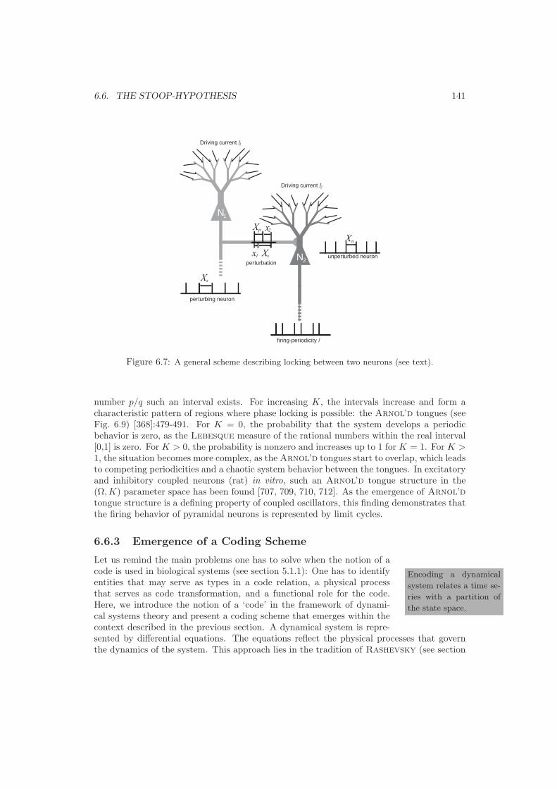
6.6. THE STOOP-HYPOTHESIS 141
Driving current I1
firing-periodicity l
N1
N2unperturbed neuron
Xu
perturbing neuron
Xs
Xp
Xs
x2
x1perturbation
Driving current I2
Figure 6.7: A general scheme describing locking between two neurons (see text).
number p/q such an interval exists. For increasing K, the intervals increase and form acharacteristic pattern of regions where phase locking is possible: the Arnol’d tongues (seeFig. 6.9) [368]:479-491. For K = 0, the probability that the system develops a periodicbehavior is zero, as the Lebesque measure of the rational numbers within the real interval[0,1] is zero. For K > 0, the probability is nonzero and increases up to 1 for K = 1. For K >1, the situation becomes more complex, as the Arnol’d tongues start to overlap, which leadsto competing periodicities and a chaotic system behavior between the tongues. In excitatoryand inhibitory coupled neurons (rat) in vitro, such an Arnol’d tongue structure in the(Ω,K) parameter space has been found [707, 709, 710, 712]. As the emergence of Arnol’d
tongue structure is a defining property of coupled oscillators, this finding demonstrates thatthe firing behavior of pyramidal neurons is represented by limit cycles.
6.6.3 Emergence of a Coding Scheme
Encoding a dynamical
system relates a time se-
ries with a partition of
the state space.
Let us remind the main problems one has to solve when the notion of acode is used in biological systems (see section 5.1.1): One has to identifyentities that may serve as types in a code relation, a physical processthat serves as code transformation, and a functional role for the code.Here, we introduce the notion of a ‘code’ in the framework of dynami-cal systems theory and present a coding scheme that emerges within thecontext described in the previous section. A dynamical system is repre-sented by differential equations. The equations reflect the physical processes that governthe dynamics of the system. This approach lies in the tradition of Rashevsky (see section

142 CHAPTER 6. DEFINING PATTERNS
Stimulus Response
Alphabet oftime series
Alphabet ofpartition
Inputtokens
Outputtoken
fc
tc
Typelevel
Tokenlevel
Semanticlevel
Partitioned state space
a
b
c
Y(T )0Y(t)
System trajectoryb
ca
behavior
System reconstructionthrough time series
Figure 6.8: Scheme describing the coding problem in the framework of dynamical systems theory.
3.2.6) and assumes real-valued mathematics as a correct basis for describing the systemunder investigation. In this way, the type level of the general coding scheme (Fig. 6.2 willbe divided into two sub-levels, a real-valued (i.e. the analytical description of the system)and a rational-valued one (i.e. the numerical description of the system, see Fig. 5.1). In thefollowing, in order to simplify notation, we assume that the system is described by a singlevariable y(t). The goal of system reconstruction is to obtain the differential equation thatgoverns the dynamics of y(t): y(t) = f(y(t), a), where a stands for a set of parametersthat determines the systems dynamics. System reconstruction is done by measuring y(t):
Definition 6.15 A measurement of a real-valued variable of a dynamical system y(t) is afunction M(y) : R → Q with
M(y(t)) = y∗(t) such that y∗(t) ∈ [y(t), y(t + δt)) ∧ y∗ ∈ Q
whereas δt is called sampling rate.
For capturing the dynamics of the system, the measurement is performed during a certaintime interval. The coarse graining imposed on the measured variable by the sampling rateof the measurement process generates symbol strings called time series:
Definition 6.16 A time series y = y1, . . . , yL that emerges by measuring a real-valuedvariable of a dynamical system y(t) during the interval [T1, T2] with sampling rate δt is thesymbol string
y∗(t1), . . . y∗(tL) with ti = δt(i − 1) + T1, i = 1 . . . L and L =T2 − T1
δt

6.6. THE STOOP-HYPOTHESIS 143
Time series are symbol strings where the symbols (= numbers) indicate the value of a cer-tain parameter at a certain time interval. Based on time series, experiments with appropriateparameter setting as well as prior knowledge on the physics of the system (i.e. assumptionsabout the physical laws that govern the dynamics) allow to obtain (in the optimal case) thedifferential equations that govern the dynamics of the system. These equations reflect thedimensionality of the state space (e.g. if y(t) describes the displacement of a simple 1D os-cillator with a single parameter (spring constant), then the state space is two-dimensional).If an analytical solution is not possible (which is the usual case when analyzing complexsystems), the embedding theorem is used for state space reconstruction [536, 635]. If weassume, that such a reconstruction has been successfully performed: What is a ‘code’ in sucha framework? Note, that the level of description of the system changed: What is referred to‘input tokens’ and ‘output tokens’ on the type level is now unified in a complete descriptionof the system. What remains to be ‘coded’? The answer to this question is: the behaviorof the system, i.e. the succession of states. We explain this point in more detail: The stateof a system is a point in the state space and the dynamics of the system is reflected by atrajectory in the state space. There now might be special regions in the state space, e.g. inthe sense that the system stays for a significant amount of time in that region. Then thestate space can be partitioned so that ‘special regions’ are separated from each other andeach part of the partition is labelled with a symbol. Whenever a trajectory enters such asymbolically labelled part of the state space, the symbol is reported and a new and simplersymbol string is generated that describes the dynamics of the system. This is the basic ideaof encoding a dynamical system [708]. In practical applications, encoding a dynamical sys-tem means to transform the time series (a symbol string) into a symbol string that emergesfrom the labelling of the partitioned state space. This string we call state series. We againassume that a single variable y(t) describes the behavior of the system and denote the stateof the system with Y (t). Then, the generation of the state series is defined as follows:
Definition 6.17 For a time series y where M(y(t)) = y∗(t) determines the state Y (t), t0 isthe beginning of the measurement and Π = πi, i ∈ N is a partition of a state space labelledby symbols of the alphabet A, a state series is the symbol string obtained by the followinginductive rule:
• Anchorage: For y∗(t0), find πi such that Y (t0) ∈ πi and report the symbol ai thatlabels πi
• Induction step:
1. For the time kδt, let Y (kδt) ∈ πi. If for (k +1)δt the condition Y ((k +1)δt) ∈ πi
is still fulfilled, repeat step 1, otherwise go to step 2.
2. Find πj = πi such that Y ((k +1)δt) ∈ πj and add the symbol aj to the string thatlabels πj. Go back to step 1, using πj instead of πi in the condition.
The state series allows the connection between the type level and the semantic level of ourcoding scheme: A specific behavior of a system as a reaction to a certain stimulus is expressedin the succession of states the system passes through in order to perform this behavior. Thissuccession of states need not always be the same, but should rather be described as a setof similar state sequences. Take the Drosophila courtship as an example: Here the courting
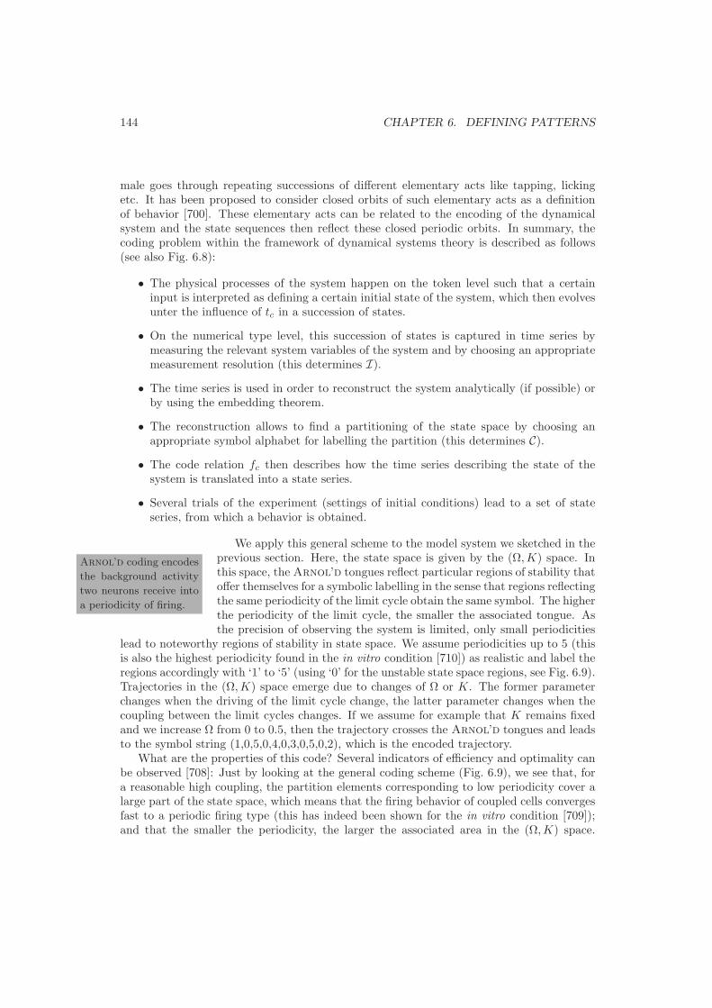
144 CHAPTER 6. DEFINING PATTERNS
male goes through repeating successions of different elementary acts like tapping, lickingetc. It has been proposed to consider closed orbits of such elementary acts as a definitionof behavior [700]. These elementary acts can be related to the encoding of the dynamicalsystem and the state sequences then reflect these closed periodic orbits. In summary, thecoding problem within the framework of dynamical systems theory is described as follows(see also Fig. 6.8):
• The physical processes of the system happen on the token level such that a certaininput is interpreted as defining a certain initial state of the system, which then evolvesunter the influence of tc in a succession of states.
• On the numerical type level, this succession of states is captured in time series bymeasuring the relevant system variables of the system and by choosing an appropriatemeasurement resolution (this determines I).
• The time series is used in order to reconstruct the system analytically (if possible) orby using the embedding theorem.
• The reconstruction allows to find a partitioning of the state space by choosing anappropriate symbol alphabet for labelling the partition (this determines C).
• The code relation fc then describes how the time series describing the state of thesystem is translated into a state series.
• Several trials of the experiment (settings of initial conditions) lead to a set of stateseries, from which a behavior is obtained.
Arnol’d coding encodes
the background activity
two neurons receive into
a periodicity of firing.
We apply this general scheme to the model system we sketched in theprevious section. Here, the state space is given by the (Ω,K) space. Inthis space, the Arnol’d tongues reflect particular regions of stability thatoffer themselves for a symbolic labelling in the sense that regions reflectingthe same periodicity of the limit cycle obtain the same symbol. The higherthe periodicity of the limit cycle, the smaller the associated tongue. Asthe precision of observing the system is limited, only small periodicities
lead to noteworthy regions of stability in state space. We assume periodicities up to 5 (thisis also the highest periodicity found in the in vitro condition [710]) as realistic and label theregions accordingly with ‘1’ to ‘5’ (using ‘0’ for the unstable state space regions, see Fig. 6.9).Trajectories in the (Ω,K) space emerge due to changes of Ω or K. The former parameterchanges when the driving of the limit cycle change, the latter parameter changes when thecoupling between the limit cycles changes. If we assume for example that K remains fixedand we increase Ω from 0 to 0.5, then the trajectory crosses the Arnol’d tongues and leadsto the symbol string (1,0,5,0,4,0,3,0,5,0,2), which is the encoded trajectory.
What are the properties of this code? Several indicators of efficiency and optimality canbe observed [708]: Just by looking at the general coding scheme (Fig. 6.9), we see that, fora reasonable high coupling, the partition elements corresponding to low periodicity cover alarge part of the state space, which means that the firing behavior of coupled cells convergesfast to a periodic firing type (this has indeed been shown for the in vitro condition [709]);and that the smaller the periodicity, the larger the associated area in the (Ω,K) space.

6.6. THE STOOP-HYPOTHESIS 145
0.2 0.4 0.6 0.8 1
0.2
0.4
0.6
0.8
1
0
0 0
1 123 34 45 5 5 5
Ω
K
Trajectory
Region A
Region B
Figure 6.9: Scheme describing Arnol’d coding in the (Ω, K) parameter space. Only areas of lock-
ing up to periodicity 5 are shown and labelled. Note, that real Arnol’d tongues (from periodicity
2 on) have curved boundaries. For further explanations, see text.
The simplest firing mode (periodicity 1) corresponds to the largest partition element in thestate space, which means that the periodicity-1 firing is most common. As (for an equalbackground activity) periodicity-1 firing is also the ‘shortest codeword’ (the sequence of thepattern only covers one ISI), the coding has a Huffman-optimality property – the mostcommon ‘codeword’ is also the less resource-intensive (in terms of the time span to ‘recognize’the ‘codeword’) and is associated to the most stable Arnol’d tongue [437].11 If we considerthe ‘biological’ background of Ω, further interesting indicators can be observed. We remindthe relation Ω = Xs/Xu. As the general noise level determines Xs (of the perturbing neuron)and Xu of the perturbed neuron, a homogeneous change of the network activity affecting thenoise level for both neurons in the same way does not change the state. Only the emergenceof a local gradient moves the trajectory and changes the state sequence. This is plausible, aslocal changes should induce such differences. Also LTP or LTD can have a role in changingthe background activity a neuron perceives, if a substantial number of (distal) synapses thatprovide the background changed their synaptic strength due to this effect. Learning in thispicture means for example, that the perturbing neuron gets a larger current inflow, increasesthe cycle time of its limit cycle and thus changes the periodicity of the output spike train ofthe perturbed neuron – which results in a change of the state sequence (‘something has beenlearned’). As the effect of synaptic plasticity on the single neuron-neuron coupling is small(the EPSP increases only in the order of 50%) it might be more reasonable to speculate, thatsynaptic plasticity is as a statistically relevant phenomenon than changes the sensibility ofthe neuron for its noisy background. But also a homogeneous increase in network activitycan have an influence: Then, the system is operating in a faster mode.
11Note, that for very small K, this type of optimality is not fulfilled, as the unstable regions in state space(the symbol ‘0’) cover the largest part of the state space.

146 CHAPTER 6. DEFINING PATTERNS
Changes in the parameter K, on the other hand, also can change the state sequenceone obtains. Consider the example, that the parameters K and Ω are bounded such thatonly trajectories in the region A are possible (see Fig. 6.9). No state sequence that encodestrajectories within this area can contain the symbols 2 and 1. However, if K changes suchthat the trajectories are contained in region B, this is possible, which could be related achange of the global state of the system. The biological interpretation of K is the coupling ofneurons. This coupling can, however, consist of two types: a synaptic type and a coincidence-firing type. First, the synaptic type means, that there must be a synapse sufficiently strongto provide a reasonable coupling. Assuming the correctness of the postulate of two classesof synapses in terms of release probability (see section 6.4.2), only the (fewer) ‘strong’synapses would probably provide a sufficient coupling. Synaptic plasticity would then bea mean to increase K. One has, however, take into account that even the strong synapseswill fail quite often to induce an EPSP. Burst-firing could then be a further way to obtainthe desired coupling and to change K by longer or shorter bursts. The coincidence-typeof coupling finally provides a solution of the problem, that the synfire hypothesis is only atheory that describes the stable propagation of activity - but not its role in a code relation.In this picture, the perturbed neuron is not coupled to a single neuron, but to a group ofsynchronously firing neurons. Chances in K are then expressed by the number of coincidentspikes. In that way, the proposed coding scheme integrates aspects considered in the ratecoding picture (the firing rate determines the background) and the time coding picture.
To summarize, neurons on a limit-cycle solution are able to combine noise (backgroundfiring) and precise timing in the following sense: The noise can be thought of as the drivingsource for the neuron, if it follows a central limit theorem behavior closely enough. Super-imposed on noise, the neuron emits and receives precisely timed firing events. The Arnol’d
tongue structure that emerges from the locking of two neurons provides a coding scheme,where analog information (e.g. given by the rate function of a group of neurons providingthe synaptic background) is converted into an essentially digital one, namely the periodicityof firing. Let I1 and I2 be two currents that drive neuron one and two. Then the codingscheme can be described as [699]:
currents I1, I2 → periodicity l
In this way, the amount of a current driving a neuron is coded with reference to thecurrent driving the target neuron. As the outcome, the encoded information is of analogand the coded information is of digital type. Thus, from a technical point-of-view, the codingscheme is an analog to digital converter.
6.6.4 The Role of Patterns
Three classes of firing:
random firing, pattern
firing and patterns in a
background.
What is the role of patterns within the above sketched framework? Threedifferent aspects have to be considered: First, how do the periodicitiesshow up in the in vivo condition? Second, how can the different findingsabout the existence of various kinds of patterns be related to this scheme?Third, what are the consequences of the need of a noisy background forthe types of neuronal firing one expects? The first aspect concerns thequestion, why the periodicities do not show up as regular spike trains

6.6. THE STOOP-HYPOTHESIS 147
in the in vivo condition, although experiments performed under the in vitro condition haveindeed led to regularly patterned spike trains [658, 709]. The reason is that the assumption ofquasi-stationary of the noisy input is not fulfilled in the in vivo condition, as one is less ableto maintain quasi-stationarity by choosing appropriate experimental conditions. However,the system can still be locked, if the noisy input changes in a correlated way (i.e. the ratio Ωremains constant), but this does not show up in the spike train. If one would know, how thedriving changes, one would be able to rescale the spike train and the periodicity would bevisible again. Indeed, experimental and model studies, where the change in driving is knownby the experimentator and one is able to do this rescaling, demonstrates the plausibility ofthis scenario: If Hodgking-Huxley neuron coupled via α-type synapses are driven undernon-quasi-stationary conditions, locking remains, expect for the case when the modulationsubstantially interferes with the neuron’s own firing frequency [699]. This has an importantconsequence for the design of neurophysiological experiments: Because of the strong responseand suppressed adaptation, this is the preferred experimental situation. However, it justmight miss the ‘normal’ working condition of the brain. When detailed compartment modelsare used to test, whether locking remains under non-quasi-stationary conditions, the resultis again positive [698]. Finally, in the in vitro condition, where the background driving ofboth neuron has been modulated to some degree such that Ω remains unchanged, againlocking is preserved (unpublished results of a diploma thesis of T. Geiges performed underthe supervision of R. Stoop). Recent investigations on neural background activity (seesection 6.3) indicate correlated activity that may also provide the conditions that locking ispreserved. The fact, that one does usually not see the firing periodicity in single neuronalspike trains does therefore not rule out the hypothesis. Concerning the second aspects, toalmost all types of patterns presented in our general overview (see section 6.1.1) a role withinthis framework can be attributed:
• Order patterns: They may reflect a stable network structure in noisy condition.
• Scaled patterns: They may represent firing periodicities for a changing background,where the change is slow compared to the mean ISI of the spike train under consider-ation.
• Interval patterns: They may represent firing periodicities for a quasi-static back-ground (single train interval pattern). Multi train interval pattern indicate quasi-staticfiring conditions for a group of locked neurons.
• Timing patterns: They may reflect a strong perturbation signal.
The third aspect, finally, implies the existence of reliable noise generators: neurons, thatare able to maintain uncorrelated (Poisson) firing for several stimulus conditions, whereasonly the firing rate changes. This raises the question of the physiological requirements thatsuch neurons can act as ‘noise generators’. Possible causes are a specific dendritic arboriza-tion that ‘randomizes’ a correlated input, or a low number or specific distribution of ionchannels that amplifies channel noise. Taking all three aspects together, one expects tofind three classes of firing in cortical neurons, that can be sustained for various stimulus-conditions: I) The class of randomly firing neurons, i.e. the ‘noise generators’, which es-sentially provide the energy source for the network activity. II) The class of neurons where
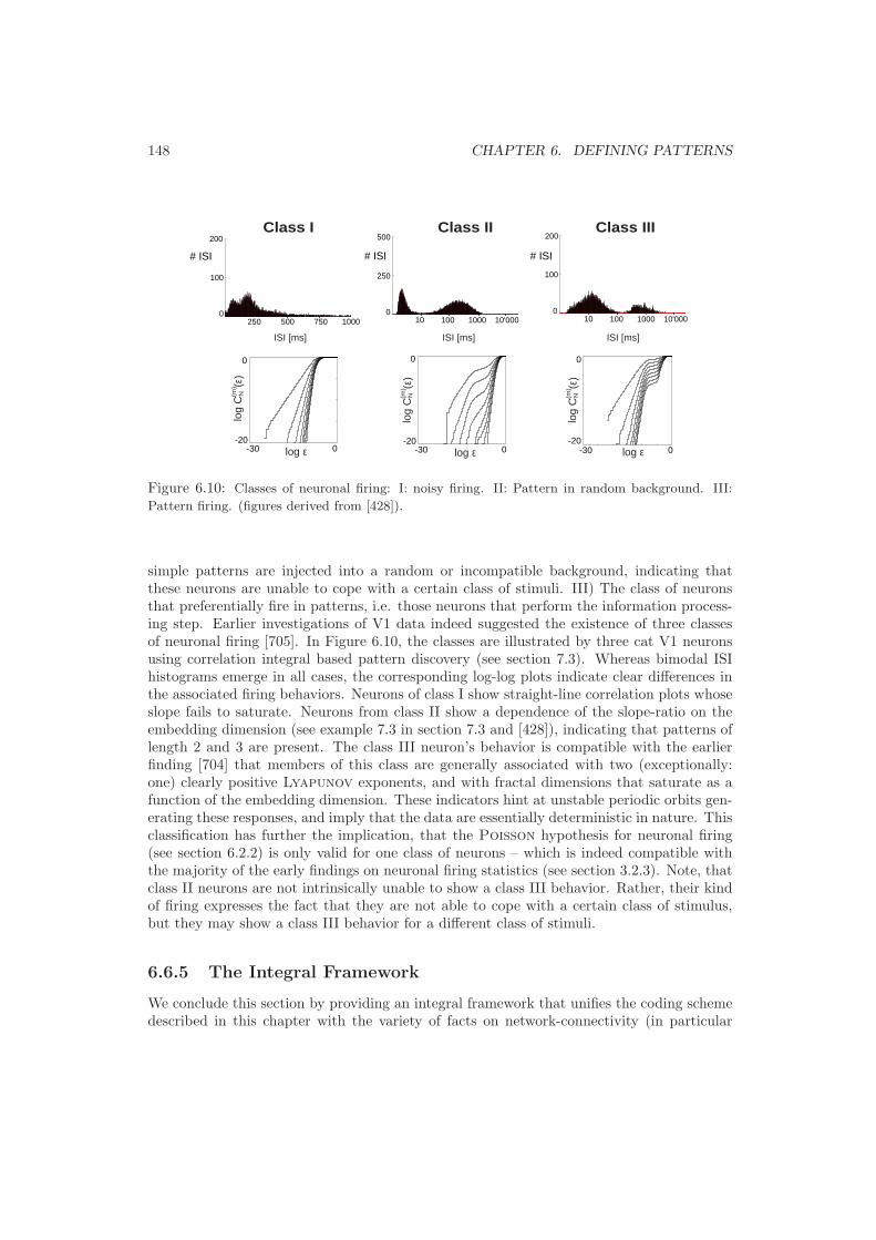
148 CHAPTER 6. DEFINING PATTERNS
0500 1000
100
200
0
250
500
10
200
0-30
0
-20
0
-200-30
0
-200-30
100
log ε log ε log ε
log
C
(ε)
(m)
N
log
C
(ε)
(m)
N
log
C
(ε)
(m)
N
Class I Class II Class III
ISI [ms]
# ISI
100 1000 10'0000
10 100 1000 10'000250 750
ISI [ms]ISI [ms]
# ISI# ISI
Figure 6.10: Classes of neuronal firing: I: noisy firing. II: Pattern in random background. III:
Pattern firing. (figures derived from [428]).
simple patterns are injected into a random or incompatible background, indicating thatthese neurons are unable to cope with a certain class of stimuli. III) The class of neuronsthat preferentially fire in patterns, i.e. those neurons that perform the information process-ing step. Earlier investigations of V1 data indeed suggested the existence of three classesof neuronal firing [705]. In Figure 6.10, the classes are illustrated by three cat V1 neuronsusing correlation integral based pattern discovery (see section 7.3). Whereas bimodal ISIhistograms emerge in all cases, the corresponding log-log plots indicate clear differences inthe associated firing behaviors. Neurons of class I show straight-line correlation plots whoseslope fails to saturate. Neurons from class II show a dependence of the slope-ratio on theembedding dimension (see example 7.3 in section 7.3 and [428]), indicating that patterns oflength 2 and 3 are present. The class III neuron’s behavior is compatible with the earlierfinding [704] that members of this class are generally associated with two (exceptionally:one) clearly positive Lyapunov exponents, and with fractal dimensions that saturate as afunction of the embedding dimension. These indicators hint at unstable periodic orbits gen-erating these responses, and imply that the data are essentially deterministic in nature. Thisclassification has further the implication, that the Poisson hypothesis for neuronal firing(see section 6.2.2) is only valid for one class of neurons – which is indeed compatible withthe majority of the early findings on neuronal firing statistics (see section 3.2.3). Note, thatclass II neurons are not intrinsically unable to show a class III behavior. Rather, their kindof firing expresses the fact that they are not able to cope with a certain class of stimulus,but they may show a class III behavior for a different class of stimuli.
6.6.5 The Integral Framework
We conclude this section by providing an integral framework that unifies the coding schemedescribed in this chapter with the variety of facts on network-connectivity (in particular

6.6. THE STOOP-HYPOTHESIS 149
inter-layer connectivity, see section 6.4.1), patterns found in sensory input to cortical layers(see section 6.5), and finally LTP and coincidence detection (see section 6.4.2). The integralframework is described in Fig. 6.11. We demonstrate using this scheme, how differentaspects of stimuli can be combined and new combinations can be learned. To keep thegeneral description simple, we do not make detailed descriptions on what exactly the stimulusconsists of. We further assume, that we are dealing with visual and auditory input. Weassume three stimuli, A, B and C. A and B may stand for different visual aspects of a singleobject, C may stand for a acoustic feature of this object, whose association to the object hasto be learned. Input on the feature A emerges from the thalamus and includes (as shownin section 6.5) multi train patterns (unitary events). This input is probably a mixture ofmulti train interval patterns, that show up as unitary events and reflect the informationabout A (see section 6.5) and uncorrelated spikes reflecting the activation of the specificpatch in the visual field. The input is sent to layer 4, where it activates a group of ‘noisegenerators’ through distal synapses, such that patterns of unitary events in the retinal inputdo not show up in the output. The uncorrelated firing of these neuron groups drive twogroups of limit cycle firing neurons: One group is again in layer 4 – which is plausible as theconnectivity between layer 4 neurons is high. This group also receives thalamic input on thestimulus A on proximal synapses. The proximal input allows spiking only if the number ofcoincident spikes emerging from the input is high enough, thus this group filters out thosespikes that are attributed to A from noisy spikes that may also be part of the input. Thesecond target group of the ‘noisy’ neurons lies in layer 2/3, where another group of limitcycle neurons is situated. The noisy input on distal synapses drives the neuron on a limitcycle solution that is associated with the general activity level of stimulus A, whereas theseneurons are perturbed by those neurons of layer 4, which filtered out the specific coincidentspikes associated with stimulus A and transmit them according to the synfire model. Theoutput of these neurons thus reflects a pattern coding for the activity level of the importantaspects of stimulus A. The same process also holds for stimulus B. For stimulus C, however,we assume that this is not the case: Although the processes in layer 4 are comparable, the‘noisy’ input of layer 4 to the group of layer 2/3 neurons is considered to be too weak toinduce limit cycle firing. The perturbation the neurons of the group obtain does thereforenot lead to a phase-locked output as described by Fig. 6.7. Thus, these neurons are class IIneurons, where only short patterns are present in a random background.
In the following, we describe, how the stimulus features A and B are combined (whichcan be considered as a solution of the binding problem) and how the binding of the featuresA and C can be learned: The A output is sent to a group of noisy neurons in layer 5,which produce again a uncorrelated output reflecting the activity of the important aspectsof stimulus A. This output is sent to three different groups of neurons: The first group ofneurons receives this input on distal synapses as a limit cycle driving current. This group isperturbed by the pattern reflecting stimulus B, such that the emerging pattern reflects thecombination of both aspects. The second group lies in layer 2/3 and targets those neurons,that are unable to cope with stimulus C. When the stimuli A and C are correlated, we expecteffects of LTP such that the synapses get stronger and the neurons changes from a class II toa class III firing. This new output is sent to neurons in layer 5, where it perturbs the limitcycle firing of another group of neuron, also driven by the noisy output representing theimportant features of stimulus A. In this way, the system has learned to associate stimuliA and C. This scheme is certainly still rather simple, but it could serve as a reference for a

150 CHAPTER 6. DEFINING PATTERNS
Laye
r 4
Laye
r 2/
3La
yer
5
ThalamusInput B
ThalamusInput A
ThalamusInput C
Output AB Output AC(after learning)
Figure 6.11: Stoop-hypothesis: integral framework. Class I neurons are in bright grey, class III
neurons are dark and class II neurons are in mid grey color. For further explanation see text
model study or to derive new experiments (see chapter 8). As we were not able to performsuch experiments, we now derive the following experimental predictions, that can be testedusing the data set that was available to us:
• Concerning the general firing statistics, we expect that only a minority of neuronsshows Poisson firing (the ‘noisy’ neurons), whereas the majority of the neurons showa deterministic behavior, which is reflected in long tail distributions.
• We expect different reliability on different stages of the information flow: The thalamicinput should display high reliability both in respect of timing and patterns. Highercortical areas should loose their timing precision but keep their pattern precision.
• We expect different clustering of neurons in terms of their pattern distance: Before thestimulus, the groups are unstable, whereas during stimuli, we expect stable groups.
• We should be able to find the three classes of neuronal firing, whereas classes I and IIIshould be larger than class II, if the set of different stimuli used is large.
• We should see differences between the stability of patterns that reflect stimulus timingnot used by the system (‘temporal coding’ according to section 5.1.2) compared topatterns that reflect computation (‘temporal encoding’): Latter should be more stable,as former are not relevant for the system.

Chapter 7
Detecting Patterns
In this chapter we outline the pattern detection problem and introduce several
methods for solving it. Conceptually, we differ between pattern discovery, pattern
recognition and pattern quantification. We review common methods for pattern
detection in spike trains. As limiting the bias for pattern detection is one of the
main requirements for any method applied in this respect, we introduce several
methods that fulfill this requirement and compare them to classical ones.
7.1 The Problem of Pattern Detection
7.1.1 Outlining the Problem
Three basic concepts:
Pattern discovery, pat-
tern recognition and pat-
tern quantification.
There is a close relation between the method used for finding patterns indata and the pattern one actually finds. Prior knowledge is introducedin several ways in the task of pattern detection: by the experimentalsetup (e.g. which stimuli are considered as ‘important’), the measure-ment (e.g. by choosing a certain measurement resolution), uncertaintiesin determining the events that are considered important (e.g. spikes orbursts, see section 6.1.2), the time span before and after the stimulus thatis considered relevant, the method used for pattern detection, and the background selectedto confirm the existence of a pattern [439, 490]. As consequence, patterns can remain un-observed due to an observer’s bias. Any method for pattern detection should minimize thebiases it introduces and should be aware of the remaining ones.1 When one looks for pat-
1Data obtained from neuronal systems furthermore suffer in many cases from a sampling problem: Onlya very small fraction of, mostly large, neurons can actually be measured in order to obtain spike data. Multielectrode array recordings and spike trains obtained using voltage-sensitive dyes may diminish this problemto a certain degree, but even today’s technology is confronted with the problem that only a small part ofa neuronal network of interest can actually be measured. This sampling problem gains importance whenlooking at multi train patterns [353]: Since only a limited number of neurons is examined, any multi trainpattern found may be part of a larger pattern which involves neurons that are not under investigation. It isthus possible, that different patterns are associated with the same subpattern.
151

152 CHAPTER 7. DETECTING PATTERNS
terns in a certain set of data, different concepts come into play: pattern discovery, patternrecognition and pattern quantification. The term pattern discovery is used, when no as-sumptions about the probability of appearance pi,j of events forming a certain pattern, thevariation of inter-event intervals ∆Xi,j or jitter ∆Ti,j are made. The term pattern recogni-tion is used, when such assumptions are indeed made – e.g. by predefining a template.2 Theterm pattern quantification is used, when the number of patterns is determined and com-pared with the number that is present in the data after choosing a certain randomizationmethod. Certainly, also pattern discovery and pattern recognition include the comparisonwith randomized data, although the conclusion whether patterns are present or not may notrely on a quantification but, for example, on a comparison between two graphical displays.For some questions (e.g. determining the reliability of neuronal firing), whole spike trainsare compared. This leads to the idea of a distance measure that is used to quantify thedifference (or similarity) between spike trains.
7.1.2 Pattern Detection Methods: Overview
Any pattern detection method relies on an appropriate description of the spike data. Usually,the spike trains are analyzed in the timing, the interval, or the bitstring representation (seesection 5.1.1). After choosing an event type which is considered as important for the problemunder investigation, the spike trains are translated into symbol strings of the particularevents that conserve the timing (or only the order) of the events. These strings are objectof the analysis. If patterns of joint spike activity in a set of simultaneously recorded spiketrains are subject to investigation, then the data set may also consist of bitstrings acrossthe trials. This means, that for a certain bin τi one checks for each train j = 1, . . . , S if aspike appears in this bin at position j. If this is the case, one writes ‘1’, otherwise ‘0’. Theresult of this procedure are sequences of bitstrings of length S representing the joint-spikeactivity [510, 514].
The first statistical methods used for pattern discovery were histogram-based (see section3.2.3). This approach relies on the counting of events, or sequences of events, available in thedata. We will discuss and classify histogram-based methods in more detail in the followingsection. A second method for pattern discovery relies on the correlation integral [428, 429].This method will be discussed in more detail in section 7.3. A further approach for patterndiscovery relies on the concept of the ε-machine [671, 670]. As input, single spike trainstransformed into bitstrings are used. The method finds the minimal hidden Markov modelthat is able to generate the bitstring. Pattern recognition methods rely on prior informationabout the potential pattern condensed in a template, which predefines the sequence and thematching interval. Template methods are widely used in spike train analysis [353, 444, 720],and also provide a way for pattern quantification. We will discuss them in more detail insection 7.4. When multi train patterns are in the focus of the analysis, the number of possiblepatterns becomes very large – especially when interval or timing patterns are considered. Toovercome this problem, usually only order patterns [559] or synchronous firing are considered.The restriction to unitary events is common, as several theoretical frameworks are availableto discuss the obtained results (the synfire hypothesis or the temporal correlation hypothesis,
2We note, that the term ‘pattern recognition’ is also widely used in the field of neural networks. Herethe term denotes the classification-ability of neural networks [558].
7.1. THE PROBLEM OF PATTERN DETECTION 153
see section 6.4.1). Several methods are available to deal with such patterns. Usually, thedata are transferred to bitstrings that represent the joint spiking activity (see above) and theassumption of independent firing is taken as null hypothesis [511, 514] (for a refinement of themethod that takes non-stationarity into account see [509, 510], for an older approach usingthe joint firing rate see [93]). Recently, several sophisticated methods that take higher orderinteractions into account (conditional inference [513], log-linear models [600], information-geometric measures [615]) have been proposed. These methods, however, face the practicalproblem that many possibilities have to be taken into account what makes the calculationcomputationally expensive. Furthermore, a large amount of individual trials is required,that often cannot be obtained in neuronal experiments. One of the few methods able to dealwith multi train interval patterns is the T-pattern algorithm, a method originally proposedfor the analysis of behavioral data [586].
T-Patterns: The T-pattern algorithm spots multi train interval patterns of singlespikes (see Def. 6.8), whereas all spikes of single patterns emerge from different neurons.The algorithm starts with a pairwise comparison of spike trains. Let t1, . . . , tn andt∗1, . . . , t∗n be such a pair. For a spike ti a so-called ‘critical interval’ [ti + ta, ti + tb],where ta < tb, is determined, so that no other spike of the first train is in the interval[ti, ta] and the number of spikes within the critical interval of the second spike train issignificantly higher than expected (Poisson null hypothesis, see below). The bordersta and tb are chosen so that there is a single spike of the second train that fulfillsti + ta ≤ t∗j ≤ ti + tb and that the probability that this happens per chance is belowa certain significance level. The expected number of spikes in the critical interval isbased on the assumption that the spikes of both trains emerge from two non-correlatedPoisson processes. To obtain longer patterns, the patterns resulting from all pairwisecomparisons of spike trains are considered singular events (hierarchical approach). Theprocedure is repeated, until a predefined hierarchical level is reached. The algorithmdelivers all patterns that are significant in the above defined sense and the number ofrepetitions of each such pattern. A method for finding multi train interval patternsthat is related to the T-pattern algorithm is based on Fisher’s exact probability test[486] – a computationally expensive method as soon as longer patterns are considered.The built-in way of randomization may be problematic for some applications. Testsperformed by us show that Poisson randomization leads to higher number of patternsin spike trains compared with ISI shuffling. When the T-pattern algorithm has beenapplied to data sets (rat olfactory bulb, see section 8.1.1) and the minimal number ofpattern occurrence has been set high (50), the number of different patterns found inthe ISI shuffled set was in the order of 50%–80% of the number found in the unshuffledset. When the minimal number of occurrence has been set low (5), still 25%–30% of thepatterns remained in the shuffled set. As we showed in section 6.2.3, the homogeneousPoisson randomization is probably uneligible for interval patterns as the degree ofrandomness introduced is too high and disregards the known statistical dependencies ofsucceeding spikes. It is therefore recommendable not to use the built-in randomizationprocedure in the Theme algorithm in order to analyze T-patterns, but to randomizethe data separately using ISI shuffling, is interval patterns are subject of analysis.
7.1.3 Spike Train Distance Measures: Overview
Spike train distance measures allow to quantify the similarity of neuronal firing. This allowsthe solution of two problems of spike train analysis. First, it provides a tool for classifying
154 CHAPTER 7. DETECTING PATTERNS
neurons. In this way, information on the functional connectivity of the probed neuronalnetwork can be gained from multi-electrode array recordings, or the distance may serve asa population criterium (see definition 5.11). Second, it provides a measure of the reliabilityof neuronal firing by calculating the mean distance of spike trains obtained in trials of thesame experiment. The larger the mean distance, the less reliable the neuron’s firing is.The similarity of neuronal firing is quantified by using measures usually called ‘distances’,although the fulfillment of the axioms of a metric (a distance is always ≥ 0, symmetric andsatisfies the triangle inequality) is seldom checked. We nevertheless speak of spike traindistance measures. A variety of distances has been proposed (see Figure 7.1):
• Spike count distance: This measure considers spike trains as similar if they have asimilar number of spikes (or, more generally, events). If L is the number of spikes inthe first train t and L∗ is the number of spikes in the second train t∗, then the distanceis defined as d(t, t∗) = |L−L∗|
maxL,L∗ . Temporal structure is not taken into account.
• Firing rate distance: For the firing rate distance, the measurement interval overwhich a spike train has been sampled is partitioned into segments of width Trate. Foreach segment, the local firing rate is calculated and the spike train is transformed insequences of rate values. The distance of two such sequences r1, . . . rn and r′1, . . . r′nis defined as
∑i(ri−r′i)
2. One may also calculate the difference of the two (continuous)approximate firing rate functions obtained by the shifting window approach. The timewindow has to be predefined.
• Cost-function distances: A family of spike train distance measures is based on theso-called ‘metric space analysis’ [742, 741]. The basic idea is to define a cost-functionthat determines the costs of transforming one spike train into another by moving,deleting and inserting spikes. The cost function has to be predefined.
• Correlation distances: Correlation distances refer to the correlation of spike trains,i.e. expressed by the hight of the highest peak in the pairwise cross-correlogram oftwo spike trains [748] or by synchronized activity measured by the so-called gravi-tational clustering approach [495, 496, 573]. Another correlation distance is basedon a convolution of a spike train with an exponential or gaussian kernel. The dis-tance is then calculated either as the integral over the difference of the convolvedtrains [737] or as the normalized dot product of the convolved trains [663]. The lat-ter correlation distance – in the following referred as C-distance – is calculated asd(t, t∗) = 1 − f(t)·f(t∗)
‖f(t)‖‖f(t∗)‖ , where f(t) denotes the convolved train. This distancemeasure requires prior information by determining the width of the Gaussian kernel.
• Information distances: Information distances are applied on spike trains in thebitstring representation. Here, several different concepts exist, relying on the Kullback-Leibler distance [532] or the Kolmogorov complexity [386]. The latter proposal emergesfrom DNA sequence analysis [570] and basically compares the lengths of the shortestdescriptions of two bitstrings representing spike trains. Another distance proposesto use the average change in the bitstring representations of a given spike train forincreasing bin-with [628]. The change is measured as the mean of the number ofsymbol-switches per bit-coded spike train. In this measure, spike trains with similar
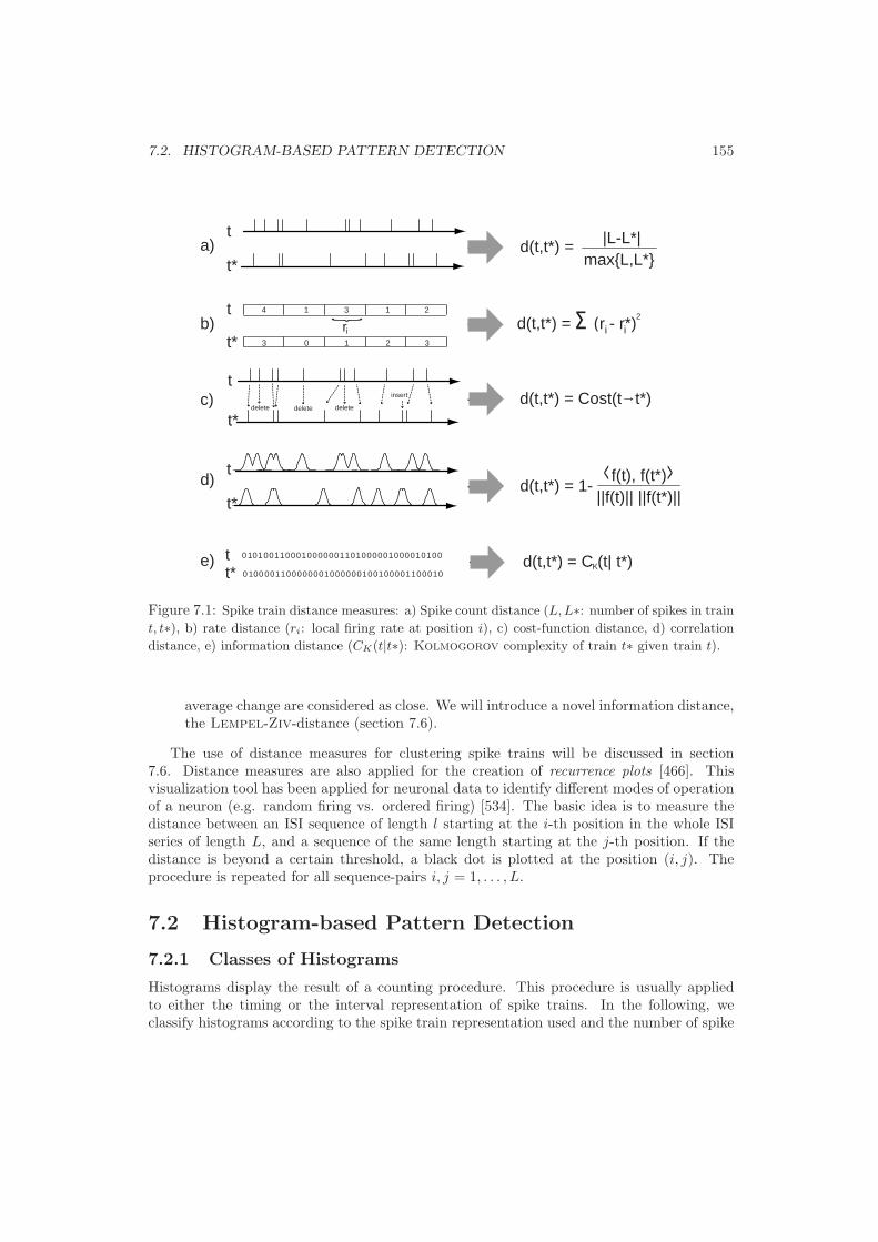
7.2. HISTOGRAM-BASED PATTERN DETECTION 155
4 1 3 1 2
3 0 1 2 3
insert
delete deletedelete
0 101 11 1 11 1 1 1 100 000 000000 0 00000 0000 0 00
0 100 11 0 00 0 0 0 000 000 000100 0 10010 0011 0 10
a)
b)
c)
d)
e)
i
ri
2
K
i
d(t,t*) =
d(t,t*) = Σ (r - r*)
d(t,t*) = Cost(t t*)
d(t,t*) = C (t| t*)
maxL,L*|L-L*|
d(t,t*) = 1- ||f(t)|| ||f(t*)||
f(t), f(t*)>>
t
t*
t
t*
t
t*
t
t*
tt*
Figure 7.1: Spike train distance measures: a) Spike count distance (L, L∗: number of spikes in train
t, t∗), b) rate distance (ri: local firing rate at position i), c) cost-function distance, d) correlation
distance, e) information distance (CK(t|t∗): Kolmogorov complexity of train t∗ given train t).
average change are considered as close. We will introduce a novel information distance,the Lempel-Ziv-distance (section 7.6).
The use of distance measures for clustering spike trains will be discussed in section7.6. Distance measures are also applied for the creation of recurrence plots [466]. Thisvisualization tool has been applied for neuronal data to identify different modes of operationof a neuron (e.g. random firing vs. ordered firing) [534]. The basic idea is to measure thedistance between an ISI sequence of length l starting at the i-th position in the whole ISIseries of length L, and a sequence of the same length starting at the j-th position. If thedistance is beyond a certain threshold, a black dot is plotted at the position (i, j). Theprocedure is repeated for all sequence-pairs i, j = 1, . . . , L.
7.2 Histogram-based Pattern Detection
7.2.1 Classes of Histograms
Histograms display the result of a counting procedure. This procedure is usually appliedto either the timing or the interval representation of spike trains. In the following, weclassify histograms according to the spike train representation used and the number of spike

156 CHAPTER 7. DETECTING PATTERNS
trains involved (see Table 7.2.1). We start with some preliminary remarks on binning : Thecounting requires a binning of the time axes. Let T be the time interval covering the wholemeasurement (timing representation of the spike train) or the length of the longest interval(interval representation of a spike train). Binning means, that a bin-size ∆τ is chosen suchthat n∆τ = T (n is the number of bins). In principle, it’s also possible to use bins of variablesize. Take the example of a timing representation of a spike train t1, . . . , tk. . . . , tl, . . . tL:The number of spikes tk, . . . tl for which (i−1)∆τ ≤ tk ≤ . . . ≤ tl < i∆τ represent the valueof the i-th bin. The choice of ∆τ depends on the problem under investigation.
Histograms of single spike trains, timing representation: These are the concep-tually most simple histograms. Several possibilities emerge. If the histogram ranges over thewhole measurement, then the histogram obtained is similar to the local rate representationof a spike train (see section 5.1.1). In case of a periodic stimulus, or some intrinsic period-icity present within the single spike train, a histogram over this period can be obtained –the phase histogram. It serves as a tool to analyze phase locking. One can also determine atime interval T ∗ and count the spike times from the first spike of the train t1 until t1 + T ∗.If this is repeated for all spikes, one obtains the auto-correlogram. It serves as an estimationof the autocorrelation function.
Histograms of multi spike trains, timing representation: A histogram over sev-eral spike trains originating from many trials of the same experiment is called post-stimulustime histogram (PSTH) or peri-stimulus time histogram. It serves as an estimation of thefiring rate function. Also the phase histogram can be obtained from many spike trains in thesame way as for single spike trains. If, however, a periodic sequence of stimulus-occurringtimes serves as a reference to count the spike times of two spike trains simultaneously, oneobtains several variants of joint-peri-stimulus histograms: The original proposal was thejoint peri-stimulus-time scatter diagram [99] which can also be displayed in the same way asa 2D interval histogram (see below). An improvement of the joint peri-stimulus-time scatterdiagram is called joint peri-stimulus diagram [359, 494]. Furthermore, a similar constructionas the auto-correlogram is possible for two different spike trains, where the spike-times ofone train serve as reference for counting the spike-times of other spike trains. The resultinghistogram is called cross-correlogram. It estimates the cross-correlation function and servesas a tool to investigate the mutual dependence of spike trains and to derive their underlying(functional, not anatomical [608]) connectivity (e.g. shared input vs. synaptic connection)[179]. If this procedure is applied for two spike trains originating from the same neuron(different trials of the same experiment), it serves as a tool to differ between stimulus-driven and intrinsic oscillations. Intrinsic oscillations show up as periodic structures in theauto-correlogram but disappear in the cross-correlogram of different trials, whereas thesestructures remain if the oscillations emerge from the stimulus (shift-predictor). Anotherapplication of the cross-correlogram is the information train technique [487]. The basicidea of this approach is, to first generate the cross-correlogram and then to build a spiketrain using only those spikes contributing to the main peaks of the cross-correlogram. Thecharacteristics of the new train is its time-locked relationship with the original train. Thecross-correlogram technique can also be extended to three spike trains. This joint impulseconfiguration scatter diagram displays the relative timing of nerve impulses in 3 simulta-neously monitored neurons [354, 175]. The time intervals between impulses are plotted ontriangular coordinates. This technique allows to analyze various connectivity patterns ofthree neurons and serves as a method to detect interval patterns of length 2 [355].

7.2. HISTOGRAM-BASED PATTERN DETECTION 157
timing representation interval representation
Timing of trial: local rate Interval histograms of order nsingle train Periodic timing: phase histogram and dimension m.
Timing relative to spikes: Scaled histogramsauto-correlogram Local trend histogram
Timing of many trials, one neuron: post-stimulus time histogram
Cross-interval histograms of or-der n and dimension m
Timing of stimulus-occurrence, two neurons:joint peri-stimulus histogram
multi train Timing relative to spikes of different trials, oneneuron: shift-predictor.Timing relative to spikes of two neurons:cross-correlogramTiming relative to spikes of three neurons:joint-impulse configuration scatter diagram
Table 7.1: Overview of histograms of single/multi spike trains in timing/interval representation.
Histograms of single and multi spike trains, interval representation: In thisrepresentation, histograms of different order and different dimension are distinguished:
Definition 7.1 For a spike train in the interval representation x1, . . . xL, a histogramthat displays the result of counting the occurrences of the n-th order intervals
n∑k=1
xk, . . . ,L∑
k=L−n
xk
in the spike train is called a n-th order histogram.
Creating a set of ISI that contains all n-th order intervals up to a certain nmax allowsthe search for interval patterns where additional spikes are allowed. The 1D histogramof all intervals between spikes up to a certain maximal time interval is called cumulativehistogram [714]). The set of all n-th order intervals can also serve as basis for other methodsfor pattern discovery, e.g. the correlation integral based method (see next section). Fordefining m-dimensional histograms, we introduce the procedure of embedding, a standardprocedure in nonlinear dynamics [458, 536, 635, 657, 716]:
Definition 7.2 For a spike train in the interval representation x1, . . . xL, the points ξ(m)k
ξ(m)k = xk, xk+1, . . . , xk+(m−1), k = 1, . . . , L − m + 1
are called embedded points and m is called the embedding dimension.
Definition 7.3 For a spike train in the interval representation x1, . . . xL, a histogramthat displays the result of counting the occurrences of intervals embedded in dimension m
ξ(m)1 , . . . , ξ
(m)L−m+1
is called a m-dimensional histogram (mD histogram).

158 CHAPTER 7. DETECTING PATTERNS
0 1000 2000 3000 4000
1000
500
0 50 10020 40 600
20
40
60
6 %13 %45 %36 %
xi
x i +1
a)
b)
c)
T [ms]
x [ms]i
# x i
Figure 7.2: Example of a 2D interval histogram: a) Spike train of a noisy, unstable neural oscillator.
b) 1D histogram of the spike train. c) 2D histogram. Gray-scales indicate the percentage of points
lying in the corresponding region of the plot.
Example 7.1: Consider the ISI series x1, x2, x3, x4, x5. The second order interval
histogram counts the intervals x1 + x2, x2 + x3, x3 + x4, x4 + x5. The 2D histogram
counts the sequences (x1, x2), (x2, x3), (x3, x4), (x4, x5). A second-order 2D histogram
counts the sequences (x1 + x2, x2 + x3), (x2 + x3, x3 + x4), (x3 + x4, x4 + x5).
The most common interval histogram is the first order 1D histogram [356], on whichthe Tuckwell classification scheme is based (see below). The first order 2D histogram –also called joint ISI histogram, scatter diagram, scatter plot, or return plot [201, 674, 675]– serves as a simple tool for pattern detection (see below). First order 3D histogram arealso used occasionally, although the graphical display is more complex [464]. Histogramsof higher dimensions can not any more be displayed. The correlation integral analysisoffers an alternative to deal with higher dimensions (see next section). Rarely used arethe scaled histogram (a histogram of the intervals between every 2m-th spike, where m is apositive integer [201]) and the local trend histogram (a histogram that counts the sequencesof differences of succeeding ISI of length 3 (xi+1 − xi, xi+1 − xi+2, xi+2 − xi+3) [482]). Inprinciple, it is also possible to consider histograms of intervals between spikes of differentspike trains. Due to practicability, this approach is usually restricted to the comparison oftwo spike trains. The first-order histogram of intervals between the spikes of two spike trainsis called cross interval histogram [179]. The sum of all cross interval histograms (usually upto a certain upper bound) corresponds to the cross-correlogram.
2D Interval Histograms: The 2D interval histogram of variable order is a convenienttool for interval pattern detection. It is able to take the serial order of intervals intoaccount, can easily be displayed, allows to estimate the length of the pattern, and a(preliminary) quantification when the histogram is displayed as a contour plot [97]. Tointroduce the 2D histogram in more detail, we use model data generated by a noisy(σ of additive gaussian noise: 2 ms) unstable neuronal oscillator that switches betweenperiodicity-1 (ISI: 30 ms) and periodicity-2 firing (ISI-sequence: (20,45) ms). In thefirst order 2D histogram, five different point clusters emerge, that are indicated bytheir centers of gravity (30,30), (20,45), (45,20), (30,20) and (45,30). The differencesin point-density are displayed by the contour plot. The gray scalings represent thepercentage of points that lie in the corresponding region compared to the total number

7.2. HISTOGRAM-BASED PATTERN DETECTION 159
of points displayed in the plot (Fig. 7.2). By systematically increasing the order ofthe 2D-histogram, information about the length of patterns is obtained: Assume thatthe ISI sequence x1, . . . xl is repeatedly present in a spike train. In the first-order2D histogram, l − 1 clusters with centers of gravity of the form (xi, xi+1) for i =1, . . . , l − 1 will be present. In the second order 2D-histogram, l − 2 clusters withcenters of gravity of the form (xi, xi+2) will be present. Proceeding in this way, thenumber of clusters diminished up to the l-th order 2D-histogram where only the clusterwith center of gravity (x1, xl) remains. Thus, this procedure allows to estimate thelength of a pattern. Figure 7.3 demonstrates this by using a spike train obtained by aPoisson spike generator with refractory period. In the spike train, the interval pattern(15, 2), (27, 2), (39, 2) has been inserted (see Def. 6.8). The first order histogramdisplays the two clusters with centers of gravity (15, 27) and (27, 39). The second orderhistogram displays only one cluster with center of gravity (42, 66). In the third-orderhistogram, no large cluster is visible.
To demonstrate the potential for pattern detection using the 2D histogram on realspike data, we display the result from four data files derived from extracellular fieldpotential measurements of neurons from the primary visual cortex of macaque monkey(data description see section 8.1). Three files (Fig. 7.4 a,c,d) derive from complex cellsstimulated with drifting gratings (drift frequency 6.25 Hz), one file (Fig. 7.4 b) derivesfrom a simple cell stimulated with drifting gratings of frequency 12.5 Hz. In Fig. 7.4.a,a regular structure of point clusters is visible (∼40% of the points belong to theseclusters), whose centers of gravity are roughly described as (9n1, 9n2), n1, n2 ∈ N –indicating a high frequency periodic firing, which is corroborated by calculating theFourier-spectrum of the spike train (data not shown). The large clusters in Fig 7.4.bresult from the drift frequency of the grating, which is reproduced by the firing of thesimple cell – a robust indicator for the identification of simple cells [682]. The 2Dhistogram reveals fine-structure within the large clusters – indicating periodic firing ofhigh frequency. In Fig. 7.4.c, ∼20% of all ISI pairs are described by the expression (a, b)and (b, a), where a ∼1 ms and b ∈ (0, 20] ms – indicating the presence of patterns in thetrain (compared to a Poisson background). Fig. 7.4.d displays the 2D histogram of aspike train that shows an exponential decay in the 1D-histogram and a cv of 1.02. As
28% 44% 28%
50
50
0
x
x
k+1
k
39% 36% 25%90
90
0 (x + x )i i+1 k
(x +
x
)j
j+1
k+1
22% 61% 17%
150
90
0 (x + x + x )i i+1 i+2 k
(x +
x
+ x
)
jj+
1
j
+2
k+
1
first order second order third order
Figure 7.3: Using the order of 2D histograms for pattern length estimation: The first order 2D
histogram of a spike train with a pattern of length 3 leads to two clusters, the second-order histogram
to one cluster and in the third order histogram the large cluster disappears. The gray-scale code
shows the percentage of points that lie in the corresponding region.

160 CHAPTER 7. DETECTING PATTERNS
10 20 30 40 50
10
20
30
40
50
0
19 %24 %39 %
x i +1
x i
a) 18 %
20 40 600
20
40
60
x i
x i +1
19 %22 %39 %
20 %
20 40 60 80 1000
20
40
60
80
100
c)
b)
3000
300
x i
x i +1
13 %23 %41 %22 %
20 40
20
4020 %20 %22 %17 %
21 %
0x i
x i +1
d) 50
30
10
3010 50
Figure 7.4: 2D histograms for neuronal data (macaque V1): a) Point clusters indicating high
frequency oscillation. b) Fine-structure in point clusters resulting from drifting grating stimulation
of simple cells indicating high frequency oscillation. c) High probability of a specific (symmetric)
firing pattern d) Firing of Poisson type cell shows no specific structures.
the 2D histogram does not indicate a serial dependence of the ISI, one may concludethat a Poisson process is a valid statistical model of the spike train.
7.2.2 1D Interval Histograms
The 1D interval histogram is (beside the PSTH) the most common histogram in neuroscience.We therefore briefly discuss the Tuckwell classification scheme for 1D histograms [732]and introduce a measure to distinguish exponential histograms from long-tail histograms.The Tuckwell classification scheme distinguishes 10 classes (see also Fig. 7.5):
1. Exponential distribution: Indicating very large EPSPs with Poissonian arrivingtimes being transformed on a one-to-one basis to action potentials.
2. Gamma-like distribution: Indicating an absolute and relative refractory period inneuronal firing. Probably only a few EPSPs occurring in a short time interval aresufficient to make the neuron firing, whereas inhibition is unlikely.
3. Gaussian distribution: Indicating that a large number of EPSPs is necessary toinduce spiking, whereas significant inhibition is unlikely.

7.2. HISTOGRAM-BASED PATTERN DETECTION 161
1) Exponential
2) Gamma
3) Gaussian
4) Delta
5) Long-tail
6) Uniform
7) Exponential, linear combination
8) Bimodal A
8) Bimodal B
8) Bimodal C
9) Multi-modal A
10) L-shaped
9) Multi-modal B
Figure 7.5: The Tuckwell classification scheme. The histograms were obtained using model data.
4. Delta-like distribution: Indicating intrinsic oscillatory firing behavior (e.g. pace-maker cells).
5. Long-tail distribution: Indicating a significant amount of inhibition. For the dis-tinction between exponential distributions and long-tail distributions see below.
6. Uniform distribution: Indicating a cell in different firing states such that the dis-tribution is the linear combination of several densities.
7. Linear combination of exponential distributions: Indicating a change of statein firing of type 1.
8. Bimodal distributions: Several kinds are distinguished: 8A indicates burst firing,8B could result from a change in firing state of type 2, and 8C indicates the presenceof two clearly distinguishable length scales possibly due to periodic stimulation.
9. Multi-modal distributions: Indicating periodic stimulation. One distinguishes be-tween low-frequency (A) and high frequency (B) stimulation.
10. L-shaped distribution: Indicating a cell in different firing states whereas one suchstate is bursting.

162 CHAPTER 7. DETECTING PATTERNS
5 10 20 50 100 2001
510
50100
500
100 200 500 15001
2
5
10
20
50
100
F (2): -7
Exp(t)Pow(t)
Exp(t)Pow(t)
x i x i
# x i# x i
a) b)
log F (2): 5log
Figure 7.6: Comparing exponential vs. power-law fits of distributions (log-log plots): a) Fitting a
exponential distribution. b) Fitting a long-tail distribution.
The distinction between exponential and long-tail distributions is of interest, as lattermay indicate a power-law that describes the firing of the neuron. The observation of power-law distributions can have far-reaching consequences. For example, for the typically observeddecay exponent, the expectation (or mean) does not exist, making it impossible to speak of amean interspike interval. Power-law decaying probability distributions indicate the presenceof long (time-)correlations as exemplified, e.g., by intermittent systems. To quantify, ifa certain distribution is closer to a exponential or a long tail type, we use the followingprocedure: Let Ni be the number of ISI that fall into the i-th bin τi (i = 1, . . . , n) of thehistogram approximating the probability distribution. To avoid tampering effects of shortISI, the bin number m with Nm = maxN1, . . . , Nn is identified. A cut-off parameterκ ∈ N determines, up to which bin number κm the left side of the distribution is removed(a reasonable choice is κ=2). For the remaining distribution, the best fits (minimizingmean square errors) of an exponential function Exp(t) = e−αt and a power-law functionPow(t) = t−α are calculated (α: fitting parameter). The fit coefficient is defined as:
Definition 7.4 For the best exponential fit function Exp(t) of the shortened distributiongiven by (τκm+1, Nκm+1), . . . (τn, Nn) and the best power-law fit function Pow(t), the fit-coefficient F(κ) is defined as:
F(κ) =1√
2(n − κm)
(n∗∑
i=κm+1
(Exp(i∆τ) − Ni)2 −n∗∑
i=2κ+1
(Pow(i∆τ) − Ni)2)
where∑n∗
i=2κ+1 indicates that the sum only goes over those bins τi where Ni = 0.
The distribution is of long-tail type for F(κ) > 0 and of exponential type for F(κ) < 0.If F(κ) ≈ 0, neither function fits the distribution well. As one fit is usually far better thanthe other, we use the logarithm Flog(κ) = sig(F(κ)) ln(abs(F(κ)), for −1 < F(κ) < 1 :Flog(κ) = 0. In Fig. 7.6.a and 7.6.b, we display two distributions generated from modelspike trains – one distribution is of exponential type, and one is of long-tail type. Thevalues of Flog(κ) obtained of this example are -7 for the exponential distribution and 5 forthe long-tail distribution.

7.3. CORRELATION INTEGRAL BASED PATTERN DISCOVERY 163
7.3 Correlation Integral based Pattern Discovery
Correlation integral
based pattern discovery
gives information on
pattern type, pattern
length and noise level.
Histogram-based tools for pattern detection require considerable effortswhen longer patterns are investigated. Furthermore, the binning intro-duces an unwanted bias, e.g. when the noise level of the system is in-vestigated. To offer an alternative for interval patterns, we introduceda unbiased statistical approach for pattern detection based on the corre-lation integral [428, 429]. The method is usually applied to spike trainsin the interval representation. If interval patterns with additional spikesare object of the analysis, then the set of all n-th order intervals up to achosen nmax is investigated.
7.3.1 The Correlation Integral
The correlation integral was originally designed for the determination of the correlationdimension [504]. In this section we explore its potential for the detection of interval patternsin spike trains. Consider a spike train in the interval representation x1, . . . xL that isembedded in the dimension m. The correlation integral is defined as follows:
Definition 7.5 For a spike train in the interval representation x1, . . . xL embedded in thedimension m, the correlation integral C
(m)N (ε) is
C(m)N (ε) =
1N(N − 1)
∑i=j
θ(ε − ‖ξ(m)i − ξ
(m)j ‖),
where θ(x) is the Heaviside function (θ(x) = 0 for x ≤ 0 and θ(x) = 1 for x > 0) and N isthe number of embedded points (N ≤ L − m + 1)
Calculating C(m)N (ε) scales with ∼ N2, making this method computationally inexpensive
compared to template-based methods (see section 7.4). Different norms ‖ · ‖ can be usedto compute C
(m)N (ε). In most cases, the maximum norm is advantageous, as this choice
speeds up the computation, and allows an easy comparison of results obtained for differentembedding dimensions. Alternatively, the Euclidean norm is used. The connection betweenC
(m)N (ε) and interval patterns is surprisingly simple: Patterns lead to clusters in the embed-
ding space. For the calculation of C(m)N (ε), an embedded point ξ
(m)0 is chosen at random.
Then, the number of points entering its ε-neighborhood is evaluated, as ε is enlarged. Ifthe chosen point belongs to a cluster, many points will join the ε-neighborhood. Once thecluster size is reached, less points are recruited, leading to a slower increase of C
(m)N (ε).
When, as required by the correlation integral, an average over different points is taken,pieces of fast increase of C
(m)N (ε) interchange with pieces of slow increase. This leads to a
staircase-like graph of the correlation integral. The denser the clustered regions, the moreprominent the step-wise structures. Plotting C
(m)N (ε) on a log-log scale not only preserves
these structures but enhances the representation of small-scale steps (in the following, weuse the logarithm over basis 2). To show the emergence of steps, we constructed a seriesfrom a repetition of the sequence 1,2,4, where the sequence numbers can be interpreted
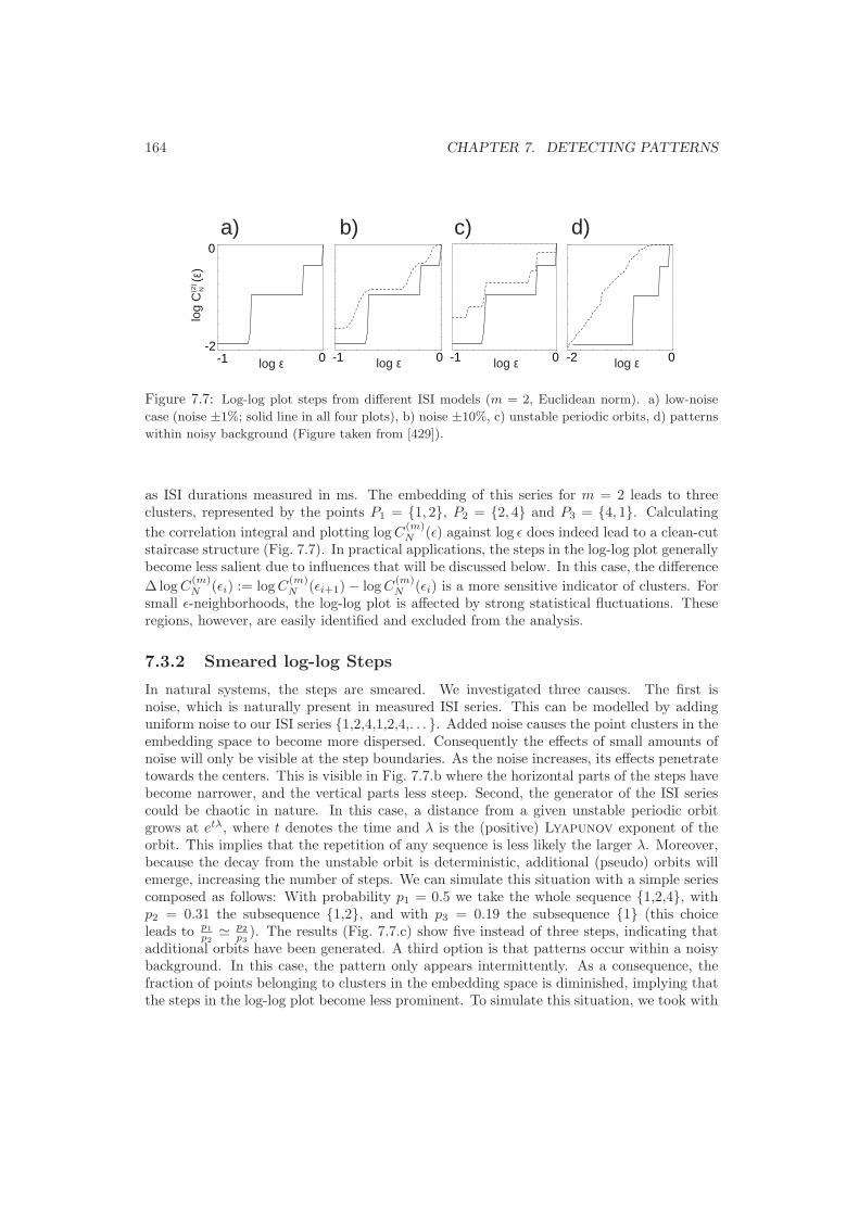
164 CHAPTER 7. DETECTING PATTERNS
-1 0 -1 0 -2 0
a) b) c)
log ε log ε log ε
log
C
(ε)
(2)
0
-2-1 0log ε
d)
N
Figure 7.7: Log-log plot steps from different ISI models (m = 2, Euclidean norm). a) low-noise
case (noise ±1%; solid line in all four plots), b) noise ±10%, c) unstable periodic orbits, d) patterns
within noisy background (Figure taken from [429]).
as ISI durations measured in ms. The embedding of this series for m = 2 leads to threeclusters, represented by the points P1 = 1, 2, P2 = 2, 4 and P3 = 4, 1. Calculatingthe correlation integral and plotting log C
(m)N (ε) against log ε does indeed lead to a clean-cut
staircase structure (Fig. 7.7). In practical applications, the steps in the log-log plot generallybecome less salient due to influences that will be discussed below. In this case, the difference∆ log C
(m)N (εi) := log C
(m)N (εi+1) − log C
(m)N (εi) is a more sensitive indicator of clusters. For
small ε-neighborhoods, the log-log plot is affected by strong statistical fluctuations. Theseregions, however, are easily identified and excluded from the analysis.
7.3.2 Smeared log-log Steps
In natural systems, the steps are smeared. We investigated three causes. The first isnoise, which is naturally present in measured ISI series. This can be modelled by addinguniform noise to our ISI series 1,2,4,1,2,4,. . . . Added noise causes the point clusters in theembedding space to become more dispersed. Consequently the effects of small amounts ofnoise will only be visible at the step boundaries. As the noise increases, its effects penetratetowards the centers. This is visible in Fig. 7.7.b where the horizontal parts of the steps havebecome narrower, and the vertical parts less steep. Second, the generator of the ISI seriescould be chaotic in nature. In this case, a distance from a given unstable periodic orbitgrows at etλ, where t denotes the time and λ is the (positive) Lyapunov exponent of theorbit. This implies that the repetition of any sequence is less likely the larger λ. Moreover,because the decay from the unstable orbit is deterministic, additional (pseudo) orbits willemerge, increasing the number of steps. We can simulate this situation with a simple seriescomposed as follows: With probability p1 = 0.5 we take the whole sequence 1,2,4, withp2 = 0.31 the subsequence 1,2, and with p3 = 0.19 the subsequence 1 (this choiceleads to p1
p2 p2
p3). The results (Fig. 7.7.c) show five instead of three steps, indicating that
additional orbits have been generated. A third option is that patterns occur within a noisybackground. In this case, the pattern only appears intermittently. As a consequence, thefraction of points belonging to clusters in the embedding space is diminished, implying thatthe steps in the log-log plot become less prominent. To simulate this situation, we took with
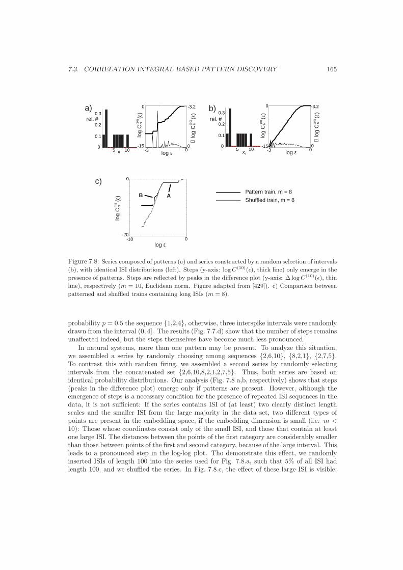
7.3. CORRELATION INTEGRAL BASED PATTERN DISCOVERY 165
0
-15
-3.2
0
log
C
(ε)
(10)
∆ lo
g C
(
ε)(1
0)
log ε
b)
NN
-3
log
C
(ε)
(10)
N
0
-15
-3.2
0
∆ lo
g C
(
ε)(1
0)
N
5 10
0.1
0.2
0.3
0.1
0.2
0.3
5 10
a)
00
0x
rel. #rel. #
ix i log ε-3 0
0
0
-10-20
AB
c)
Shuffled train, m = 8
Pattern train, m = 8
log
C
(ε)
(m)
N
log ε
Figure 7.8: Series composed of patterns (a) and series constructed by a random selection of intervals
(b), with identical ISI distributions (left). Steps (y-axis: log C(10)(ε), thick line) only emerge in the
presence of patterns. Steps are reflected by peaks in the difference plot (y-axis: ∆ log C(10)(ε), thin
line), respectively (m = 10, Euclidean norm. Figure adapted from [429]). c) Comparison between
patterned and shuffled trains containing long ISIs (m = 8).
probability p = 0.5 the sequence 1,2,4, otherwise, three interspike intervals were randomlydrawn from the interval (0, 4]. The results (Fig. 7.7.d) show that the number of steps remainsunaffected indeed, but the steps themselves have become much less pronounced.
In natural systems, more than one pattern may be present. To analyze this situation,we assembled a series by randomly choosing among sequences 2,6,10, 8,2,1, 2,7,5.To contrast this with random firing, we assembled a second series by randomly selectingintervals from the concatenated set 2,6,10,8,2,1,2,7,5. Thus, both series are based onidentical probability distributions. Our analysis (Fig. 7.8 a,b, respectively) shows that steps(peaks in the difference plot) emerge only if patterns are present. However, although theemergence of steps is a necessary condition for the presence of repeated ISI sequences in thedata, it is not sufficient: If the series contains ISI of (at least) two clearly distinct lengthscales and the smaller ISI form the large majority in the data set, two different types ofpoints are present in the embedding space, if the embedding dimension is small (i.e. m <10): Those whose coordinates consist only of the small ISI, and those that contain at leastone large ISI. The distances between the points of the first category are considerably smallerthan those between points of the first and second category, because of the large interval. Thisleads to a pronounced step in the log-log plot. Tho demonstrate this effect, we randomlyinserted ISIs of length 100 into the series used for Fig. 7.8.a, such that 5% of all ISI hadlength 100, and we shuffled the series. In Fig. 7.8.c, the effect of these large ISI is visible:

166 CHAPTER 7. DETECTING PATTERNS
Embedding dimension m
1 2 3 4 5 6 7
Patt
ern
size
l 1 0 0 0 0 0 0 02 1 1 1 1 1 1 13 3 2 1 1 1 1 14 6 4 3 2 2 2 25 10 8 6 4 2 2 26 15 12 9 7 5 3 3
Table 7.2: Maximum number of steps s(m, n) as a function of the embedding dimension m and
pattern length l.
For m = 8, the pronounced step A emerges in the patterned series as well as in the shuffledseries, whereas the smaller steps B emerging from the sequences are not present in theshuffled train. Remember that the question whether step A should count as an indicationof a pattern depends on the chosen background. If not ISI shuffling, but a homogeneousPoisson background is considered as relevant, then the appearance of a particular lengthscale is also considered a pattern.
7.3.3 Pattern Length Estimation
Once the presence of patterns has been established, an estimate of the pattern length canbe given. That this is possible is motivated by the following argument. Using the maximumnorm, the distance between two points is defined as the largest coordinate difference. An in-crease of the embedding dimension yields ever more coordinate pairs, causing the presence ofa particularly large difference to dominate. Consequently, the number of steps calculated forpattern length l decreases with increased embedding dimension m. The maximum numberof steps s(l,m) can be numerically computed as follows. We start from a series generated bya repetition of a sequence of length l. Additionally, we require that the elements x1, . . . , xlyield distinct coordinate differences |xi − xj |. After choosing an embedding dimension m, ldistinct embedded points are generated. On this set of points, the maximum norm inducesclasses of equal inter-point distances. The number of these classes equals s(l,m). The ac-tual calculation of s(l,m) can be done using a computer program (which exhausts ordinarycomputer capabilities very quickly), or by an unexpectedly involved analytical calculation[620]. The lowest numbers s(l,m) are given in Table 7.2. They clearly confirm the antic-ipated decrease of the number of steps as a function of m. For the series generated fromthe sequence 5, 24, 37, 44, 59, our correlation integral approach is able to reproduce thepredicted decrease of s(l,m) (Fig. 7.9.a): In embedding dimension m = 1, all ten possiblenonzero differences are visible. As m increases towards 5, the number of steps decreases inaccordance with Table 7.2, remaining constant for m > 5.
The behavior reported in Table 7.2 only holds if the series are created by repeatinga pattern based on distinct inter-coordinate differences. In more general cases, the exactdetermination of the pattern length is hampered by a basic difficulty: If one single stepemerges, this can either be due to a interval pattern of length 2 or two interval patterns of

7.3. CORRELATION INTEGRAL BASED PATTERN DISCOVERY 167
length 1. A greater number of steps further complicates this problem. As a consequence,Table 7.2 can only serve as a rough guideline. Fortunately, a helpful indicator for the patternlength exists. A pattern will emerge in the embedded ISI series in its most genuine form (itis neither cut into pieces, nor spoilt by foreign points) if the pattern length equals the chosenembedding dimension (l = m). In Fig. 7.9.a, the most pronounced steps appear at m = 5,correctly indicating a pattern of length l = 5. To investigate the reliability of the criterionin natural settings, noise was added to the series generated from the sequence 5, 24, 37,44, 59. For the following, we define the noise strength as the ratio of the noise samplinginterval over the shortest sequence interval. The results (Fig. 7.9 b-f) demonstrate that thepattern length can be reliably estimated up to a noise level of 512% (Fig. 7.9.e), where themost pronounced step still appears at m = 5. The number of steps for m < 5 is affected bythe noise: For m = 1, for example, 9 steps are present at 8% noise (Fig. 7.9.b), 7 steps at32% (Fig. 7.9.c) and 3 steps at 128% (Fig. 7.9.d). The step-structure disappears, if the noiselevel reaches the size of the largest sequence element (Fig. 7.9.f). Thus, the observation thatthe most pronounced step appears at l = m, yields a valuable criterion for estimating thepattern length.
We found that this criterion also extends to less ideal settings. To illustrate, we injectedthe sequences 5, 25, 10, 2 and 5, 25, 10, 2, 17, 33, each with probability p = 0.06, into anoisy background generated by a homogeneous Poisson process with refractory period. ThePoisson distribution was tuned to produce a mean identical with that of the patterns. The
log ε
log
C
(ε)
(m)
N
log ε
log
C
(ε)
(m)
N
0
-3
a) b)m = 1
m = 2
m = 3
m = 4
m = 5-8
c)
d)
-4-4-3
0 e) f)
0 0
log ε-4 0
Figure 7.9: Dependence of step appearance from noise level. a): The number of steps decreases
as the embedding dimension increases (m = 1, . . . , 8; sequence length: 5). At m = 1 there are 10
steps, in agreement with Table 7.2. b-f): Behavior in the presence of additive noise (noise levels
8%, 32%, 128%, 512% and 1024%, see text). The number of steps for m = 1, . . . , 4 decreases for
increased noise. The clearest step always emerges for m = 5, indicating a sequence of length 5
(Figure taken from [429]).

168 CHAPTER 7. DETECTING PATTERNS
0-20
0
-200-20
a) b) c)
log ε log εlog ε
log
C
(ε)
(m)
m = 4 m = 6
m = 3
m = 4
-15 0-15
0
N
0
-20
Figure 7.10: Pattern-length indicator l = m: Sequences of length n in a homogeneous Poisson
background (embedding dimensions m = 1, . . . , 8): a) l = 4 – most pronounced step at m = 4; b)
l = 6 – most pronounced step at m = 6. c) Sequences of l = 3 and l′ = 4 included with different
ratios (3 : 1 solid line, 1 : 3 dashed line) – most pronounced step where m equals the length of the
dominating sequence (Figure taken from [429]).
clearest steps emerge at the embedding dimensions 4 and 6 (Fig. 7.10.a,b) showing that alsoin this case the pattern length can be estimated. We refined our investigation by varying theinjection probabilities. Using the sequences 4, 17, 12 and 5, 25, 10, 2, the first sequencewas chosen with p = 0.12 and the second with p = 0.04. We compared this series witha series based on interchanged probabilities. The outcome shows that the clearest stepsemerge for m = n where the pattern with the higher probability dominates (Fig. 7.10.c). Ifthe two probabilities are similar, the estimation may be hampered by effects of interference.A means of quantifying the ‘clarity’ of a step, is to calculate the ratio between the slopes ofthe flat and of the steep part of the steps. Consistently, the embedding dimension for whichthe slope-ratio reaches a minimum coincides with the pattern length.
Currently, alternative models of noisy backgrounds exist. To show that our results holdregardless of the model applied, we injected the sequence 33, 14, 22 into backgrounds gen-erated by a) a homogeneous Poisson process with refractory period, b) an inhomogeneous,sinusoidally modulated Poisson process with refractory period, and c) a uniform randomprocess on the interval (0, 46], using injection probabilities p ∈ 0, 0.03, 0.09, 0.15. The re-sults show that the nature of the noisy background has a negligible influence on the patterndetectability. Instead, the injection probability is decisive (Fig. 7.11). Whereas two sharp
m 1 2 3 4
fm
sm0.27 0.19 0.20 0.30
Table 7.3: Ratio of the flat slope (fm) over the steep slope (sm) of a step, as a function of the
embedding dimension m, of the data shown in Fig. 7.12.

7.3. CORRELATION INTEGRAL BASED PATTERN DISCOVERY 169
0
0.08
0
0.08
0
0.08
c)b)a)p = 0
p = 0.03
p = 0.09
p = 0.15
log ε-10 0 -10 0 -8 0
∆ lo
g C
(ε
)(3
)
0
0.08
N
Figure 7.11: Detection of sequences injected (with p = 0, 0.03, 0.09, 0.15) into random backgrounds
based on the difference quotient: a) Homogeneous Poisson background, b) inhomogeneous Pois-
son background, c) uniform background. Already at a low injection probability of p = 0.03, a
hump emerges (dashed boxes). At p = 0.09, smaller peaks indicate the statistically significant
accumulation of pattern-induced distances (m = 3) (Figure taken from [429]).
peaks are obtained for p = 0.15 and p = 0.09 (arrows), only one large hump emerges forp = 0.03. A single broad peak indicates a reduced frequency of short intervals, which is thefirst indicator of patterns at lowest injection probability. Two narrow peaks indicate thepattern-generated statistically significant accumulation of particular distances.
Example 7.2: We demonstrate the use of correlation integral based pattern discoveryusing data obtained from striate cortex of cats (for details see section 8.1). First, weshow the determination of the length of interval patterns: In Fig. 7.12, we display thelog-log plot of the correlation integral for the embedding dimensions m = 1, . . . , 8 forone spike train. It can be seen that the steps are expressed differently in the differentembedding dimension. To quantify these differences, the ratio of the slope of the flatpart on the left side of the step fm and the slope of the step sm is calculated fordifferent embedding dimensions m (Table 7.3.3). This analysis reveals ratio minima atm = 2 and m = 3, indicating that patterns of length 2 and 3 are present. As a secondexample, we display the log-log plots for spike trains from a neuron under differentstimulus conditions. Here, a pattern-sharpening effect can be observed in the log-logplot [704]. These examples demonstrates how information about pattern length andnoise level can be obtained by comparing the plots for different embedding dimensions.
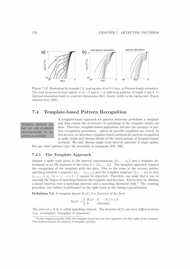
170 CHAPTER 7. DETECTING PATTERNS
-20 0-20
0
log ε
log
C
(ε)
(m)
s
f
f
f
f
s
s
s
4
4
3
3
2 2
11
N
a) b)
0-300-30
0
-20
sub-optimal stimulation optimal stimulation
log ε log ε
log
C
(ε)
(m)
NFigure 7.12: Illustration for example 7.2: Log-log plot of cat V1 data. a) Pattern-length estimation:
The most pronounced steps appear at m = 2 and m = 3, indicating patterns of length 2 and 3. b)
Optimal stimulation leads to a pattern sharpening effect, clearly visible in the log-log plot (Figure
adapted from [429]).
7.4 Template-based Pattern Recognition
Template methods are
fast, yet only if reliable
prior-knowledge of the
pattern is available.
A template-based approach for pattern detection predefines a templateand then counts the occurrence of matchings of the template within thedata. Therefore, template-based approaches fall into the category of pat-tern recognition procedures – unless all possible templates are tested. Inthis section, we introduce template-based methods for pattern recognitionin spike trains and discuss details of the shortcomings of template-basedmethods. We only discuss single train interval patterns of single spikes.
For any other pattern type, the procedure is analogous [423, 490].
7.4.1 The Template Approach
Assume a spike train given in the interval representation x1 . . . , xL and a template de-termined as an ISI sequence of the form x = x1, . . . xl. The template approach requiresthe comparison of the template with the data. Due to the noise in the system, perfectmatching between a sequence xi, . . . xi+l−1 and the template sequence x1, . . . xl so thatxj−i+1 = xj , ∀j = i, . . . i + l − 1 cannot be expected. Therefore, one must find a way toquantify the degree of matching between the template and the data. This is done by defininga kernel function over a matching interval, and a matching threshold [444].3 The countingprocedure (see below) is performed on the spike train in the timing representation.
Definition 7.6 A template kernel Kx(t) is a function of the form
Kx(t) =
K(t) if − b ≤ t ≤ b0 otherwise
The interval [−b, b] is called matching interval. The function K(t) can have different forms(e.g. rectangular, triangular or gaussian).
3In the original proposal [444], the template kernel has not been applied to the first spike of the template.This underestimates the number of template matches.

7.4. TEMPLATE-BASED PATTERN RECOGNITION 171
Definition 7.7 For a interval sequence x1, . . . xl and a template kernel Kx(t), a templateTl(t) of length l is
Tl(t) = Kx(t) +l∑
k=1
Kx
(t −
k∑i=1
xi
)
The interval sequence x1, . . . xl used to define the template is called template sequence.
Definition 7.8 For a spike train t1, . . . , tL and a template Tl(t), the matching functionM(t∗) of the template set at position t∗ of the spike train is
M(t∗) =∑
∀ti≥t∗−b
Tl(ti − t∗)
Definition 7.9 For a matching function M(t∗) and a matching threshold Mtresh, the match-ing M(t∗) of the template put at position t∗ of the spike train is
M(t∗) =
1 if M(t∗) − Mtresh ≥ 00 otherwise
Usually, the matching is calculated for succeeding values of t∗ = t∗1, . . . , t∗n and the obtained
values 0 or 1 are then written in a matching string M = M(t∗1) . . .M(t∗n).
The procedure to calculate the number of template matches is described as follows (seeFig 7.4.1): For a given spike train and a template, a bin-size ∆τ (e.g. 1 ms) and a matchingthreshold Mtresh are chosen. Then, the matching string is calculated for t∗ = i · ∆τ wherei = 0, . . . , n (n is the number of bins that cover the measurement interval of the spike train).The number of switches 0 → 1 in the matching string defines the number of templatematches. If the matching string already starts with a ‘1’, then 1 is added to the number ofswitches. Note, that this general procedure allows the detection of patterns where additionalspikes are allowed. It is certainly possible to restrict the template approach to detect intervalpatterns where no such spikes are allowed.
7.4.2 Problems with Templates
Template based methods suffer from two fundamental difficulties. First, the detection relieson the set of pre-chosen templates. As the patterns are a priori unknown, large templatesets are required that include all potential patterns. Second, a bias is introduced by choosingthe template kernel (choice of K(t) and [−b, b]). Especially the choice for a tolerance fortemplate matching is problematic. Adopted matching intervals range from fractions of one[714] to a few milliseconds [720], demonstrating the difficulty in determining the requiredaccuracy. We illustrate both aspects separately.
Combinatorial explosion: Unbiased template-based pattern detection would requiretesting all possible templates (the ad hoc method [353]). The number of operations requiredfor unbiased testing can be estimated as follows: Let x1, . . . , xL be a spike train in theinterval representation with xmin denoting the smallest and xmax the largest element. Letx1, . . . xl be the template sequence and [−b, b] be the matching interval. An optimal binsize of ∆τ = 2b yields N = xmax−xmin
∆τ values to test, and N l templates to match. Moreover,

172 CHAPTER 7. DETECTING PATTERNS
0 1 11 0
Template kernel
Template
Template matching
Matching stringgeneration
t
K(t)
tx1 x2
-b b
t*
etc. t
t
∆τ
Calculate M(t)
Figure 7.13: The basic template matching algorithm (from top to bottom): First, a template kernel
K(t) with matching interval [−b, b] is defined. Then, by choosing a template sequence x1, x2, the
template is generated. Then, after defining a matching threshold, the matching function for a
certain t∗ determined if the template matches a spike train (M(t∗) = 1 in the example). By
applying this procedure from the beginning of the spike train and for steps ∆τ , one obtains the the
matching string M. The number of switches 0 → 1 defines the number of template matches.
an unbiased template analysis requires choosing a set B of distinct matching intervals. Thisleads to ∼ lB(L− l+1)N l templates that need to be compared. The problem is aggravated,when interval patterns in multiple spike trains are target of the analysis, as the templateshave to be applied to all possible combinations of spike trains. It is evident that an efficienttemplate analysis can only be performed for small l. This problem can be reduced using thebootstrap method [353]: The basic idea is to perform the template analysis only for smalll. Longer templates are then created by using only those intervals that have been found toform short interval patterns.
Matching interval: A way to minimize the number of templates to be tested is to geta valuable estimation of the size of the matching interval: This can be obtained by applyingthe 2D histogram or the correlation integral method. If the noise that affects the patternis small the clusters in the embedding space are dense, which shows up accordingly in the2D histogram or in the slope of the steps in the correlation integral. On the other hand, bysystematically varying the matching interval for a given template, one is also able to obtainan estimation for the noise level, as the number of matchings of templates reaches a plateau
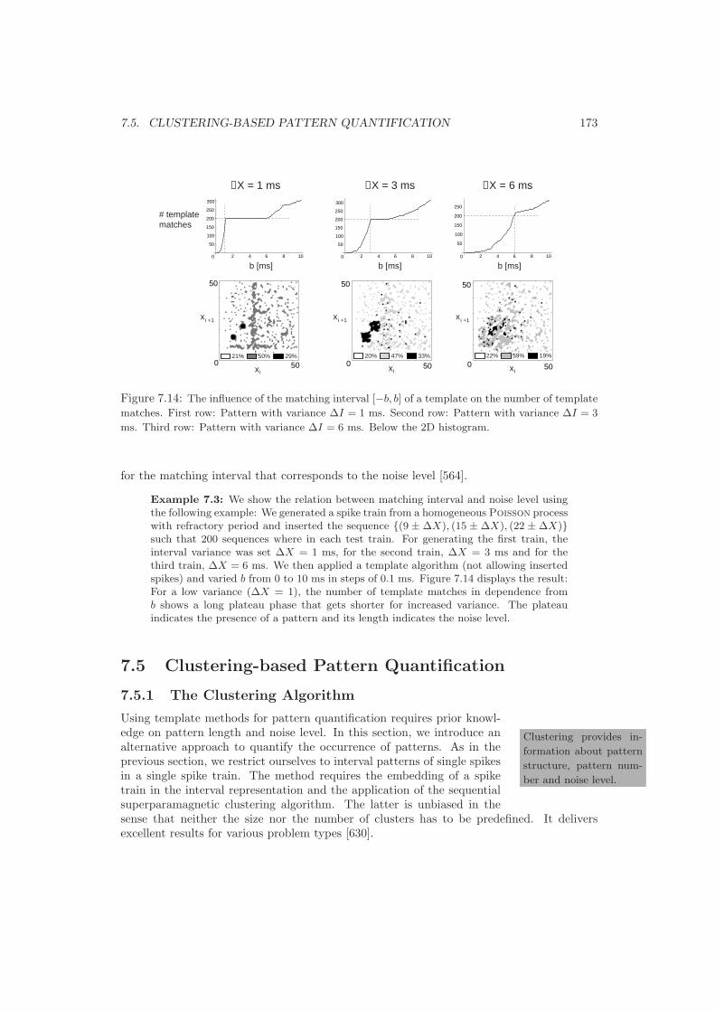
7.5. CLUSTERING-BASED PATTERN QUANTIFICATION 173
2 4 6 8 10
50
100
150
200
250
300
50
50
2 4 6 8 10
50
100
150
200
250
300
2 4 6 8 10
50
100
150
200
250
0 0 0
21% 50% 29% 20% 47% 33% 22% 59% 19%0 50
50
0 50
50
0
# templatematches
∆X = 1 ms ∆X = 3 ms ∆X = 6 ms
b [ms] b [ms] b [ms]
xi
xi +1
xi xi
xi +1 xi +1
Figure 7.14: The influence of the matching interval [−b, b] of a template on the number of template
matches. First row: Pattern with variance ∆I = 1 ms. Second row: Pattern with variance ∆I = 3
ms. Third row: Pattern with variance ∆I = 6 ms. Below the 2D histogram.
for the matching interval that corresponds to the noise level [564].
Example 7.3: We show the relation between matching interval and noise level usingthe following example: We generated a spike train from a homogeneous Poisson processwith refractory period and inserted the sequence (9 ± ∆X), (15 ± ∆X), (22 ± ∆X)such that 200 sequences where in each test train. For generating the first train, theinterval variance was set ∆X = 1 ms, for the second train, ∆X = 3 ms and for thethird train, ∆X = 6 ms. We then applied a template algorithm (not allowing insertedspikes) and varied b from 0 to 10 ms in steps of 0.1 ms. Figure 7.14 displays the result:For a low variance (∆X = 1), the number of template matches in dependence fromb shows a long plateau phase that gets shorter for increased variance. The plateauindicates the presence of a pattern and its length indicates the noise level.
7.5 Clustering-based Pattern Quantification
7.5.1 The Clustering Algorithm
Clustering provides in-
formation about pattern
structure, pattern num-
ber and noise level.
Using template methods for pattern quantification requires prior knowl-edge on pattern length and noise level. In this section, we introduce analternative approach to quantify the occurrence of patterns. As in theprevious section, we restrict ourselves to interval patterns of single spikesin a single spike train. The method requires the embedding of a spiketrain in the interval representation and the application of the sequentialsuperparamagnetic clustering algorithm. The latter is unbiased in thesense that neither the size nor the number of clusters has to be predefined. It deliversexcellent results for various problem types [630].
174 CHAPTER 7. DETECTING PATTERNS
Sequential Superparamagnetic Clustering: The conceptual idea of superparam-agnetic clustering can be outlined as follows: Data points are interpreted as particlesto which a Potts-spin is assigned. Each particle can interact via its spin with theparticles of a defined neighborhood (usually k-nearest neighbors) . The particles tendto align the direction of their spins depending on the interaction strength, whereasthermal fluctuation opposes this tendency. The interaction strength is a decreasingfunction of the distance between the points. Groups of particles with aligned spinsform clusters, whose size diminish with increasing temperature T. Groups of particleswith strong interaction are able to resist this tendency of disintegration. Thus, the sizeof this cluster is stable over a broad range of T. Clustering is applied for a certainrange of T = 0, . . . , Tend in steps of ∆T. Usually at T = 0, one cluster is present,which breaks up into smaller clusters for increasing T. The sequential approach allowsto take inhomogeneities in the data space into account: The data points of the densestcluster are removed and the clustering algorithm is reapplied to the remaining dataset as well as to the removed cluster. The application of superparamagnetic clusteringalgorithm requires the determination of several parameters. The most important onesare minsize (the minimal size of clusters) and sθ (the minimal required cluster sta-bility), which define the resolution of the clustering procedure. The other parametersare only of minor interest and basically influence the efficiency of the algorithm. Inthis way, the clustering algorithm comes equipped with an intrinsic measure for clusterstability s, with 0 ≤ s ≤ 1. It sequentially reveals clusters according to their stabil-ity, i.e. the most stable cluster is detected first and the remaining cluster is the leaststable one. The result of clustering is displayed in a dendrogram that indicates howlarger clusters break apart into smaller clusters. Furthermore, the size of the clusterN, Tmax (the temperature, where all clusters have disintegrated), the cluster stabilitys (the temperature range over which the cluster remains stable relative to Tmax), Tcl
(the temperature range over which the cluster remains stable) and Tferro (the tempera-ture, where the cluster is still in the ferromagnetic phase, i.e. all spins are aligned) aredisplayed. For a formal description of the algorithm, we refer to Ref. [629].
The superparamagnetic clustering algorithm delivers the size of a cluster and its centerof gravity, the standard deviation for each coordinate of the center of gravity and the indexnumbers of the points which form the cluster. It provides the following information:
• When stable clusters emerge, they indicate the presence of patterns (see below).
• The coordinates of the centers of gravity of the clusters provide information about theinterval pattern.
• The standard deviations of the coordinates of the centers of gravity provide informationabout the cluster density and thus about the noise level.
• By using the index numbers of the points one gains information about the exactoccurrence of the patterns within the spike train.
7.5.2 Relating Patterns and Clusters
We have already noticed (section 7.3), that interval patterns in spike trains show up asclusters in the embedding space. In this paragraph, we outline this connection in moredetail. We assume that the interval pattern (X1,∆X1), . . . (Xl,∆Xl) is present in the spike
7.5. CLUSTERING-BASED PATTERN QUANTIFICATION 175
train x1, . . . xL. Embedding the spike train leads to points ξ(m)k = (xk, . . . , xk+(m−1)),
k = 1, . . . , N , where k is the index number of the point, m is the embedding dimension andN = L − m + 1 is the number of generated points. The clusters that emerge due to thepresence of the pattern consist of points of the form ξ(m) = (Xi ± ∆Xi), . . . (Xj ± ∆Xj)where j − i = m − 1. The number of points forming the cluster equals the number ofrepetitions of the pattern in the spike train. In other words, if the embedding of a spiketrain leads to clusters in the embedding space, the centers of gravity of the clusters indicatewhat patterns may be present. The density of the clusters indicate the noise level.
We outline in the following how one infers a pattern from clusters obtained in differ-ent embedding dimensions (see also example 7.5). We assume that we have embeddeda spike train in the interval representation that contains only one unknown pattern oflength l in different embedding dimensions m = 2, . . . ,M (the case m = 1 is in mostcases uninteresting). For m = 2, l − 1 clusters will emerge, whose centers of gravity canbe described as (c1
1, c12), . . . , (c
l−11 , cl−1
2 ). In the symbol cij , i denotes the number of the
cluster and j denotes the coordinate number within each center of gravity. When (as weassume) the clusters emerge from only one pattern, they can be re-numbered such thatc12 ≈ c2
1, c22 ≈ c3
1, . . . , cl−22 ≈ cl−1
1 . For m = 3, l − 2 clusters will appear where a similarrelation can be obtained for the coordinates ci
j of the centers of gravity. For m = l, only onecluster will emerge and for m > l, no more cluster will appear. The systematic comparison ofthe centers of gravity of clusters obtained in different embedding dimensions will thus resultin the pattern present in the data (see also example 7.5 below). This approach may becomecomplicated if many different patterns are present in the data as several combinations haveto be tested. This is, however, a problem for all pattern detection methods.
Cluster stability: In practical applications the parameter stabmin provides additionalinformation on the noise level of the system: if clusters remain stable for large values ofstabmin, the noise level is low. It is, however, important to notice, that the embedding ofpatterned data will automatically lead to stable and unstable clusters. To discuss this pointin more detail, we again assume that repeating sequences of the form (X1 ±∆X1, . . . , Xl ±∆Xl) are present in a spike train. Thus, points (Xl−j+1, . . . , Xl, xi+j , . . . , xi+(m−1)) and(xi, . . . , xi+(m−1)−j ,X1, . . . , Xj), 0 < j < m and m ≤ l + 1 will emerge in the embeddingspace of dimension m, where only the first or last j < m coordinates derive from the pattern(see Fig. 7.15 as an example). These points form unstable clusters, as m − j coordinatesemerge from the random background and not from the pattern. Unstable means, that theclusters decrease rapidly in size for increasing temperature T. This fact is expressed in amuch higher standard deviation of some coordinates of the centers of gravity of unstableclusters – namely those coordinates which are not related to the pattern. Clusters relatedto patterns, on the other hand, show a substantial decrease of the standard deviation for allcoordinates of the center of gravity of the cluster at some critical temperature T′ (due tothe split of a larger cluster) and an almost constant size for a range [T′,T′′].
Example 7.4: Starting point is a ISI series provided by a uniform random pro-cess on the interval [1,20], into which the sequence (2,15,8) and all its subsequences(2, 15), (15, 8), (2), (15), (8) have been injected. Furthermore, uniform noise has beenadded to the series. Its embedding in m = 1, 2, 3 (see Fig. 7.15.a) and the application ofthe clustering algorithm resulted in several clusters. The centers of gravity of the stableclusters are (as expected) (2.0), (15.0), (8.0) for m = 1, (2.0, 15.1), (15.1, 8.0) for m = 2and (2.0, 15.0, 8.0) for m = 3 (encircled clusters in Fig. 7.15.a). The pattern group

176 CHAPTER 7. DETECTING PATTERNS
0
5 10 15 20
5
10
15
20
5 10 15 20
0
5
10
15
20
05
1015
20
0
5
1015
20
xi
xi
xi
xi+1
x i+1
xi+2
m = 1
m = 2 m = 3
a)
0
Temperature T
coor
dina
te v
alue
s
clus
ter
size
T' = 0.05
5
10
15
0.02 0.04 0.06 0.08 0.1 0.120
100
200
300
ccc
1
2
3
0.02 0.04 0.06 0.08 0.1 0.12
3
3
3
stablecluster
unstable cluster
b)
Figure 7.15: Relating patterns and clusters. a) Embedding of a spike train containing one pattern
(example 7.5) in m = 1, . . . , 3. Encircled are clusters, whose centers of gravity correspond to the
sequences forming the pattern. c) Identifying clusters related to patterns using the criterion of
cluster-stability for m = 3 (see text).
is thus reconstructed as P3 = (2), (15), (8), (2, 15), (15, 8), (2, 15, 8). Note, that onecannot expect perfect matches when comparing according coordinates of the centers ofgravity in different embedding dimensions (15.0 15.1 in the example).
To demonstrate the criterion of cluster-stability, we consider the emergence of thestable cluster indicating the sequence (2,15,8) in m = 3 (Fig. 7.15.b). In this cluster,all coordinates of the center of gravity have settled down to the values 2, 15, and 8,their standard deviations remain small and the cluster size remains largely unchangedfor 0.05 ≤ T ≤ 0.12. In clusters that emerge from points, where only the first twocoordinates emerge from the pattern, the situation is different: In the example, the

7.6. THE LZ-DISTANCE OF SPIKE TRAINS 177
third coordinate of the center of gravity changes its value considerably for increasingT, its standard deviation stays large compared to those of the other coordinates andthe cluster size also diminishes considerably for increasing T. If stabmin is chosenappropriately, these unstable clusters will not emerge as clusters in the algorithm.
As the clustering approach is able to quantify a whole pattern group, the method issuited to determine the stability of a pattern (see section 6.1.3). If, however, the number ofpatterns present in the data as well as the noise level are high, the clustering based methodmay only be used as a tool to find an appropriate template.
7.6 The LZ-Distance of Spike Trains
Spike trains with similar,
but distributed patterns
are close when measured
by the LZ-distance.
A thorough classification of spike trains requires two ingredients: Thechoice of an appropriate distance measure, and an efficient clustering al-gorithm [477]. In this section, we focus on the first step. For the secondstep, we use the sequential superparamagnetic clustering algorithm (seeprevious section). We introduce a novel distance measure based on theLempel-Ziv-complexity (LZ-complexity) [143] that does not require tun-ing parameters, is easy to implement and computationally cheap. Themeasure is applied to spike trains transformed into bitstrings and considers spike trainswith similar compression properties as close. Used in spike train clustering, the measuregroups together spike trains with similar but possibly delayed firing patterns (Fig. 7.16).This is important as neurons that receive similar input or/and perform similar computa-tions might have a tendency to respond by similar patterns. Due to the complex neuronal
a)
b)c)
d)
Input
Output
Figure 7.16: Outline of the spike train clustering problem: Multi electrode array recordings probe
the spatio-temporal activity within a neural net. Correlation-based distance measures allow to
group together spike trains with synchronous spike patterns (a,b; pattern marked with grey bar),
but fail to group trains with delayed patterns (c,d).
178 CHAPTER 7. DETECTING PATTERNS
connectivity of the cortex, similar firing patterns may occur delayed in different neurons anddistance measures focussing on synchronized firing would not be able to classify such cellsas similar. Furthermore, when firing reliability of single neurons under in vivo conditionsis considered, the measure again allows to deal with different delays of firing patterns thatmay appear in the different trials of the same experiment. Such differences may result frominfluences to the neuron under investigation that are, in the in vivo condition, beyond theexperimenter’s control. This is of special importance when the firing reliability of neuronsin higher cortical areas is considered as it is known that timing reliability, measured bydistances focussing on synchronized firing, will be lost. Thus, the LZ-distance measures anadditional aspect of neuronal firing reliability.
7.6.1 The LZ-Distance Measure
The LZ-distance measure is applied to spike trains in the bitstring representation (see sec-tion 5.1.1). This string can be viewed as being generated by a more general informationsource. For this source, we want to find the optimal coding [437]. This coding is based onparsing, a procedure to partition the string into non-overlapping substrings, according tosome procedure. Based on the concept of LZ-complexity, two distinct parsing procedureshave been introduced [143, 291]. Both of them follow the same basic idea: strings are se-quentially parsed into sequences that have not occurred. To explain the differences amongthe two procedures, we introduce the following definitions:
Definition 7.10 For a bitstring Xn = (x1 . . . xn) of length n (xi ∈ 0, 1), a procedure thatpartitions Xn in non-overlapping substrings is called a parsing. If all substrings of a certainstring Xn generated by a parsing are distinct, then the parsing is called a distinct parsing.
Definition 7.11 For a bitstring Xn of length n, a substring starting at position i and endingat position j of the string which is the result of a parsing procedure is called a phrase Xn(i, j).The set of phrases generated by a parsing of Xn is denoted with PXn
and the number of phrases|PXn
| is denoted by c(Xn)
Definition 7.12 If Xn is a bitstring of length n, the set of all substrings of Xn is calledvocabulary, denoted VXn .
Assume a bitstring Xn that has been parsed up to position i, so that PXn(1,i) is the setof phrases generated so far and VXn(1,i) is the vocabulary of the parsed substring Xn(1, i).The question is: What will be the next phrase Xn(i + 1, j)? According to the originallyproposed parsing procedure [143], it will be the first substring which is not yet an elementof VXn(1,i) (LZ-76). According to the second proposed parsing procedure [291], it will be thefirst substring which is not an element of PXn(1,i) (LZ-78). As an illustration, take the string0011001010100111. Using the LZ-76 procedure, it will be parsed as 0|01|10|010|101|00111,whereas it will be parsed as 0|01|1|00|10|101|001|11 using the LZ-78 procedure.
Definition 7.13 If Xn is a bitstring, the Lempel-Ziv-complexity K(Xn) (LZ-complexity) ofXn is defined as
K(Xn) =c(Xn) log c(Xn)
n
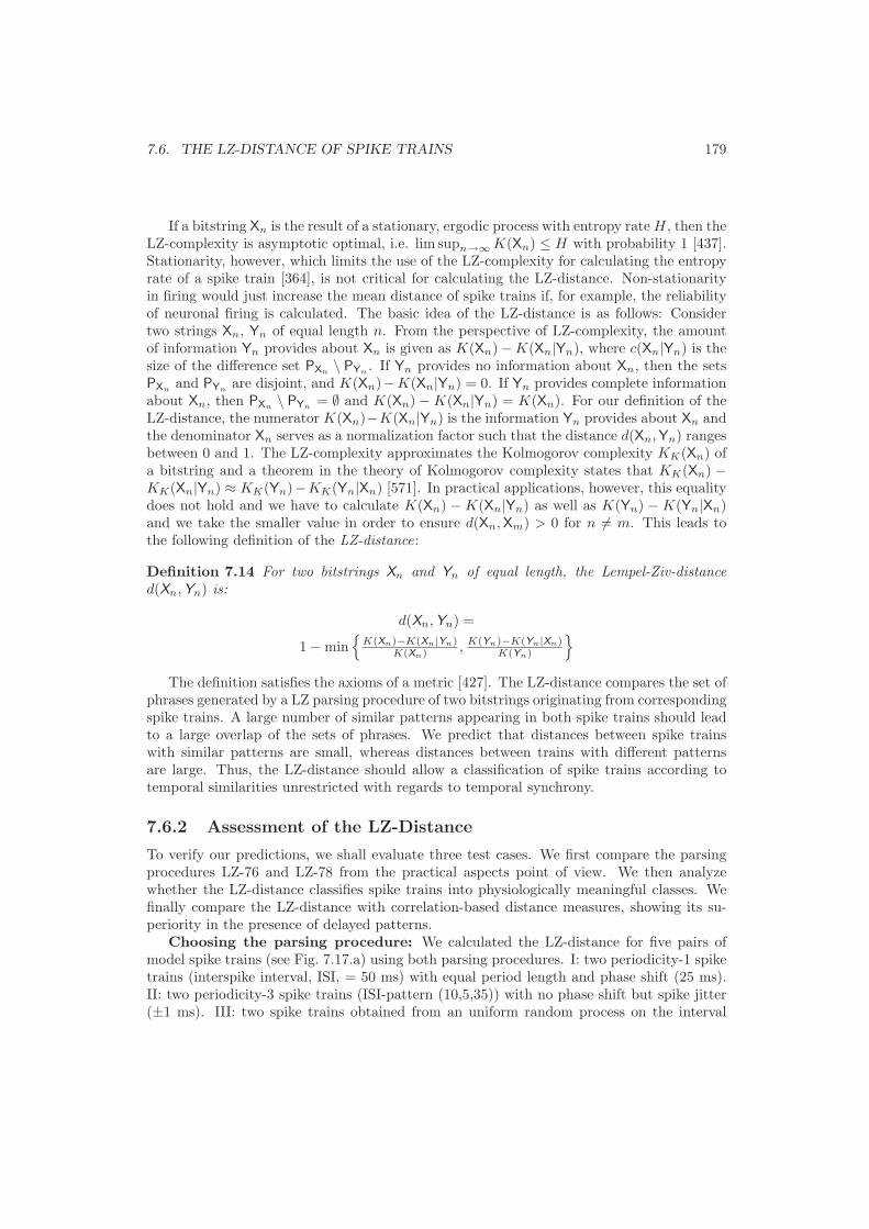
7.6. THE LZ-DISTANCE OF SPIKE TRAINS 179
If a bitstring Xn is the result of a stationary, ergodic process with entropy rate H, then theLZ-complexity is asymptotic optimal, i.e. lim supn→∞ K(Xn) ≤ H with probability 1 [437].Stationarity, however, which limits the use of the LZ-complexity for calculating the entropyrate of a spike train [364], is not critical for calculating the LZ-distance. Non-stationarityin firing would just increase the mean distance of spike trains if, for example, the reliabilityof neuronal firing is calculated. The basic idea of the LZ-distance is as follows: Considertwo strings Xn, Yn of equal length n. From the perspective of LZ-complexity, the amountof information Yn provides about Xn is given as K(Xn)−K(Xn|Yn), where c(Xn|Yn) is thesize of the difference set PXn
\ PYn. If Yn provides no information about Xn, then the sets
PXnand PYn
are disjoint, and K(Xn)−K(Xn|Yn) = 0. If Yn provides complete informationabout Xn, then PXn \ PYn = ∅ and K(Xn) − K(Xn|Yn) = K(Xn). For our definition of theLZ-distance, the numerator K(Xn)−K(Xn|Yn) is the information Yn provides about Xn andthe denominator Xn serves as a normalization factor such that the distance d(Xn,Yn) rangesbetween 0 and 1. The LZ-complexity approximates the Kolmogorov complexity KK(Xn) ofa bitstring and a theorem in the theory of Kolmogorov complexity states that KK(Xn) −KK(Xn|Yn) ≈ KK(Yn)−KK(Yn|Xn) [571]. In practical applications, however, this equalitydoes not hold and we have to calculate K(Xn) − K(Xn|Yn) as well as K(Yn) − K(Yn|Xn)and we take the smaller value in order to ensure d(Xn,Xm) > 0 for n = m. This leads tothe following definition of the LZ-distance:
Definition 7.14 For two bitstrings Xn and Yn of equal length, the Lempel-Ziv-distanced(Xn,Yn) is:
d(Xn,Yn) =
1 − min
K(Xn)−K(Xn|Yn)K(Xn) , K(Yn)−K(Yn|Xn)
K(Yn)
The definition satisfies the axioms of a metric [427]. The LZ-distance compares the set of
phrases generated by a LZ parsing procedure of two bitstrings originating from correspondingspike trains. A large number of similar patterns appearing in both spike trains should leadto a large overlap of the sets of phrases. We predict that distances between spike trainswith similar patterns are small, whereas distances between trains with different patternsare large. Thus, the LZ-distance should allow a classification of spike trains according totemporal similarities unrestricted with regards to temporal synchrony.
7.6.2 Assessment of the LZ-Distance
To verify our predictions, we shall evaluate three test cases. We first compare the parsingprocedures LZ-76 and LZ-78 from the practical aspects point of view. We then analyzewhether the LZ-distance classifies spike trains into physiologically meaningful classes. Wefinally compare the LZ-distance with correlation-based distance measures, showing its su-periority in the presence of delayed patterns.
Choosing the parsing procedure: We calculated the LZ-distance for five pairs ofmodel spike trains (see Fig. 7.17.a) using both parsing procedures. I: two periodicity-1 spiketrains (interspike interval, ISI, = 50 ms) with equal period length and phase shift (25 ms).II: two periodicity-3 spike trains (ISI-pattern (10,5,35)) with no phase shift but spike jitter(±1 ms). III: two spike trains obtained from an uniform random process on the interval

180 CHAPTER 7. DETECTING PATTERNS
200 400 6000VIVIIIIIIa)
b)t [ms]
5 10 15 20 25
0.2
0.4
0.6
0.8
1
1 2 3 40t [sec] t [sec]
0
0.2
0.4
0.6
0.8
1
d(x,y)
LZ-76 LZ-78
Figure 7.17: Distances of pairs of spike trains. a) Raster plot of pairs I-V. b) Distances of pairs
I-V in dependence from the length of the spike train for LZ-76 and LZ-78 parsing.
[1, 50]. IV: a periodicity-1 (ISI = 50 ms) and a periodicity-3 (ISI-pattern (10,5,35)) spiketrain with coincident spikes. V: two periodicity-1 spike trains with different period lengths(50 ms,15 ms). In order to analyze the convergence behavior, for LZ-76 parsing, the lengthof the trains have been increased from 100 ms up to 4000 ms in steps of 100 ms. For LZ-78parsing, the lengths of the trains have been increased from 1 sec up to 25 sec in steps of1 sec. The results (Fig. 7.17.b) show that the distance based on LZ-76 parsing convergesfaster than LZ-78 parsing. Furthermore, same pairs lead to different distances: Using LZ-76parsing, the trains I are close, the trains IV and V are rather distant and the trains II andIII are most distant. Using LZ-78 parsing, the trains I are close as well, but the trains IIand III are less close, and the trains IV and V are most distant. This demonstrates, thatthe LZ-distance based on LZ-78 parsing is more noise-robust than LZ-76 parsing. The latterconsiders similar, but noisy trains (II) as most distant, whereas the first measure considersspike trains with distinct firing behaviors (IV, V) as most distant. The evaluation of theparsing procedure explains this difference: In LZ-76 parsing, the lengths of the phrasesincrease much faster during the procedure than in the LZ-78 parsing, because |VXn(1,i)| |PXn(1,i)|. Therefore, the probability that strings obtained from two similar but noisyspike trains contain many different phrases is higher for the LZ-76 if compared to the LZ-78parsing. As noise robustness is important when dealing with neuronal data, LZ-78 is bettersuited for practical purposes, also because it is computationally cheaper.
Spike train classification: To test whether the LZ-distance sorts spike trains in phys-iologically meaningful categories, we generate a set of spike trains with in vivo and modeldata of comparable firing rate (80-90 spikes/second), as it is obvious that groups of spiketrains that differ in firing rate are easily recognized using the LZ-distance. Our multi traindata set contains five classes with nine spike trains of 2400 ms length each. Class A: Spiketrains of a complex cell (macaque monkey visual cortex data, for further explanation seenext section) driven by drifting gratings of 6.25 Hz. Class B: Spike trains of a simple celldriven by drifting gratings of 12.5 Hz. Class C: Spike trains of a homogeneous Poisson
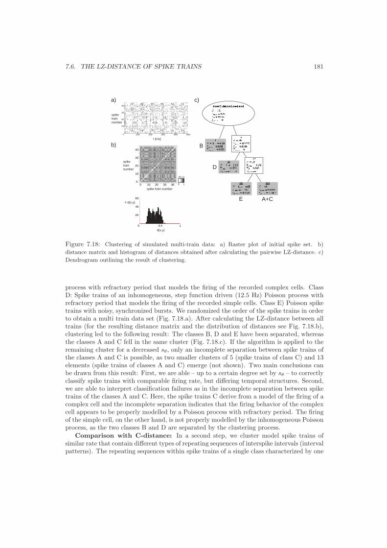
7.6. THE LZ-DISTANCE OF SPIKE TRAINS 181
spike trainnumber
100 200 300 400 500
10
20
30
40
0
t [ms]
0 10 20 30 400
10
20
30
40
0 0.5 1
20
40
60
spike trainnumber
d(x,y)
# d(x,y)
b)
spike train number
d(x,y)
0 1
a) c)
B
D
E A+C
Figure 7.18: Clustering of simulated multi-train data: a) Raster plot of initial spike set. b)
distance matrix and histogram of distances obtained after calculating the pairwise LZ-distance. c)
Dendrogram outlining the result of clustering.
process with refractory period that models the firing of the recorded complex cells. ClassD: Spike trains of an inhomogeneous, step function driven (12.5 Hz) Poisson process withrefractory period that models the firing of the recorded simple cells. Class E) Poisson spiketrains with noisy, synchronized bursts. We randomized the order of the spike trains in orderto obtain a multi train data set (Fig. 7.18.a). After calculating the LZ-distance between alltrains (for the resulting distance matrix and the distribution of distances see Fig. 7.18.b),clustering led to the following result: The classes B, D and E have been separated, whereasthe classes A and C fell in the same cluster (Fig. 7.18.c). If the algorithm is applied to theremaining cluster for a decreased sθ, only an incomplete separation between spike trains ofthe classes A and C is possible, as two smaller clusters of 5 (spike trains of class C) and 13elements (spike trains of classes A and C) emerge (not shown). Two main conclusions canbe drawn from this result: First, we are able – up to a certain degree set by sθ – to correctlyclassify spike trains with comparable firing rate, but differing temporal structures. Second,we are able to interpret classification failures as in the incomplete separation between spiketrains of the classes A and C. Here, the spike trains C derive from a model of the firing of acomplex cell and the incomplete separation indicates that the firing behavior of the complexcell appears to be properly modelled by a Poisson process with refractory period. The firingof the simple cell, on the other hand, is not properly modelled by the inhomogeneous Poissonprocess, as the two classes B and D are separated by the clustering process.
Comparison with C-distance: In a second step, we cluster model spike trains ofsimilar rate that contain different types of repeating sequences of interspike intervals (intervalpatterns). The repeating sequences within spike trains of a single class characterized by one

182 CHAPTER 7. DETECTING PATTERNS
200 400 600 800 1000
10
20
0
spike trainnumber
t [ms]
0 0.5 1
15030
0 0.5 1
d(x,y) d(x,y)
# d(x,y)
a)
b)
c)
E
D
A
B C
Figure 7.19: Comparison of distance measures. a) Test trains b) Distributions of LZ-distances
(left) and C-distance. c) Dendrogram of clustering the spike train set using the LZ-distance: All
five classes are clearly recognized.
type of interval pattern are not synchronized, but randomly distributed within each train.This challenging task for spike train clustering is performed using the LZ-distance andthe C-distance ( [663], see 7.1.3), the latter is a common distance measure for spike trainclustering problems [477]. We generated five classes of spike trains, characterized by thefollowing interval patterns. Class A: (4,4), class B: (13,13,13), class C: (5,20,3), class D:(3,16,3,16), and class E: (1,4,7,2,6,11). Each spike train (five per class) was generated suchthat 50% of the interspike intervals of the train originate from the sequence and 50% froma homogeneous Poisson process. The rate of the process has been adapted for each classin order to generate almost identical mean firing rates for all spike trains (92-94 spikes persecond). The order of the spike trains was again randomized to generate our multi traindata set (Fig. 7.19.a). To this data set, sequential superparamagnetic clustering has beenapplied, using both the LZ- and the C-distance. The result shows a clear difference betweenthe two distance measures: Whereas the LZ-distance allowed a clear-cut separation of allfive classes (Fig. 7.19.c), the use of the C-distance did not lead to any classification (data notshown). This noticeable difference in performance becomes transparent, if the distributionof the distances is compared (Fig. 7.19.b). For the LZ-distance, their range is ∼0.4 witha multi-modal distribution (indicating the structure within the data set), whereas for theC-distance their range is ∼0.1 with a unimodal distribution. The latter observation impliesthat a re-scaling would not allow a performance increase. This demonstrates that the LZ-distance is a more general measure allowing to classify spike trains with delayed patterns.The usual correlation measures that focus on synchronized firing fail in such situations.

7.7. PATTERN DETECTION: SUMMARY 183
incr
ease
d bi
as
Problem type
Pattern detectionFiring reliability
within single train
comparing trials
Patternstability
Trialdistances
classificationcode relation
spike trainclustering
choosepattern type
choosebackground
spike trainrepresentation
spike trainshuffling
Distance measure:- evaluate quality of statistical null hypothesis
Correlation integral:- pattern discovery- noise level- pattern length (if dominating pattern)
Clustering:- pattern quantification- noise level- pattern elements
Histograms:- pattern discovery- noise level- pattern length (if dominating pattern)- pattern elements
Templates:- pattern quantification- noise level - pattern length- pattern elements
Figure 7.20: The pattern detection problem: Overview of problem types and methods.
7.7 Pattern Detection: Summary
We conclude this chapter by providing an integrative overview of the presented pattern de-tection methods. We distinguish two basic problem types: The reliability of firing discussionand the pattern detection problem. The problem of firing reliability subdivides in two cases:First, the question to what extent spike trains of several trials of the same experiment differ(see section 6.3.3). Second, the question to what extent a single neuron fires reliably duringa certain period. The adequate way to solve the former problem is to define an appropri-ate distance measure and to calculate the distances of the different trials. The higher thevariance of the distances, the less reliable is the firing. The latter problem is solved bycalculating the pattern stability (see section 6.1.3).
The pattern detection problem can also serve two purposes: First, classifying sets ofspike trains according to similarities in firing. Second, detecting patterns and putting themin a coding/computation framework. The first sub-case, the spike train clustering problem,relies on the choice of a distance measure and a clustering algorithm (see section 7.6). Thesecond sub-case requires a more detailed analysis: One first has to determine the pattern

184 CHAPTER 7. DETECTING PATTERNS
type of interest, which leads to an appropriate transformation of the original data (section6.1.1). If for example burst patterns are of interest, then one transforms a spike trainin a series that indicates only the occurrence times of bursts, neglecting the occurrencetimes of single spikes. Second, one has to choose an appropriate way of randomization(section 6.2.3). In order to evaluate the degree of randomness introduced in the data,the distance between the original train and the shuffled train can be calculated, using anappropriate distance measure. Third, one has to choose the appropriate method by takingcare of the bias they introduce: The correlation integral based pattern discovery is lessbiased than the histogram-based approaches (the latter needs the definition of a bin-size),although it provides a more detailed analysis about the elements of the pattern. For patternquantification, the clustering approach is less biased than the template-based approach,unless all possible templates and matching intervals are tested. The template approach,however, may allow better comparison of different data sets. The statistical significance ofthe results obtained is tested by applying the same methods to the randomized trains. Thesignificance in context of a code relation, finally, has to be evaluated in specific experiments.Figure 7.20 provides an overview of the pattern detection problem.
Chapter 8
Investigating Patterns
In this chapter we test the methods of chapter 7 and evaluate the predictions that
emerge from the Stoop-hypothesis presented in section 6.6.5: We investigate the
firing statistics in the visual system of cat and macaque monkey, and the olfactory
system of rat, we analyze the firing reliability in the visual system of the monkey,
we perform clustering of cell groups in the olfactory system, we test for patterns
in the visual system of cat and monkey, and probe the pattern stability for selected
cells in the visual system of macaque monkey.
8.1 Description of the Data
8.1.1 Rat Data: Olfactory System (mitral cells)
The rat data derive from experiment performed by Alister Nicol of the Cognitive &Behavioral Neuroscience Lab, Babraham Institute, Cambridge (UK). Neuronal activity ofanaesthetized rats was sampled by means of a micro-electrode array positioned in the olfac-tory bulb (25% urethane, intraperitoneal, 1.5g per kg body weight). Micro-electrode arrayscomprised 30 electrodes (6 × 5, 350 µm separation). Odors, carried as saturated vapors innitrogen gas (odorless), were mixed in various concentrations with dry air and were deliveredfor 10 seconds to the rat via the mask. Breathing was monitored and onset of odor deliverywas timed to mid-expiration. Neuronal activity was sampled in the 10 second period beforeodor onset (the pre-stimulus period) and the 10s period of odor presentation (the during-stimulus period). Spikes were detected when a triggering threshold was crossed by therecorded signal from each electrode. This threshold was set at ≥ 2 × the background noiselevel. The activities of single or multiple neurons were detected in the activity sampled byeach electrode. The activities of individual neurons were discriminated from multiple neuronactivity using a Kohonen network to cluster principle components derived from the actionpotential waveforms, allowing discrimination of activity from 1-6 neurons at each active site.In this way, simultaneous recordings from 54 neurons were made. Odor presentations were10s in duration. Four different odors (amyl acetate, M-Butanol, DL-camphor, cineole) were
185

186 CHAPTER 8. INVESTIGATING PATTERNS
Area Animal # cells # stimuli # files analyzedLGN cat 6 3 18
monkey 9 6-7 27V1 cat 4 3-6 17
monkey 28 5 140MT monkey 7 16 35
olfactory bulb rat 54 16 ∼5100
Table 8.1: Overview data set. All measurements have been performed in the in vivo condition
presented in four different concentrations (5.42 ×10⁻⁸ mol, 2.71 ×10⁻⁷ mol, 1.36 ×10⁻⁶
mol, 5.42 ×10⁻⁶ mol). Thus, pre- and during-stimulus recordings were made under a totalof 16 different stimulus conditions. For each condition, there were three trials, resulting ina total of 96 spike trains per neuron. The total number of files analyzed by us was ∼5100,as not all cells have been recorded in all stimulus conditions. All procedures used for datacollection conformed to the Animals (Scientific Procedures) Act, 1986 (U.K. Home Office).
8.1.2 Cat Data: Visual System (LGN, striate cortex)
The cat data used in the analysis derive from two sources: The LGN data derive fromin vivo measurement of an anesthetized cat performed by Valerio Mante and Matteo
Carandini from the Smith-Kettlewell Eye Research Institute, San Francisco (USA). Thedetailed experimental procedures are outlined in Ref. [485]. We analyzed the responses of sixcells to three classes of stimuli: sinusoidal gratings with randomly changing spatial frequencyand direction, a cartoon movie, and a natural stimulus video. Each stimulus class consistedof 2-4 different stimuli of 10-30 seconds duration. The stimuli were shown repeatedly (15-25times in randomized order). To avoid stimulus onset artifacts, the first 50 ms of each trialwere deleted. By concatenating these recordings we obtained 18 cell, and stimulus, specificISI series. The V1 data derive from a series of in vivo experiments dedicated to the study ofcontrast dependence of neural activity in cat visual cortex performed by Kevan Martin ofthe Institute of Neuroinformatics, University and ETH Zurich (Switzerland). The detailedexperimental procedures are outlined in Ref. [599], with the modifications according to Ref.[360]. An analysis of the data from our side has been published in Refs. [701, 704]. We used17 spike trains from 4 unspecified neurons from unspecified layers (12 trains display evokedactivity, 5 spontaneous activity) for our analysis.
8.1.3 Monkey Data: Visual System (LGN, V1, MT)
The monkey data derive from measurements in the LGN, V1 and area MT of macaquemonkey, performed by Adam Kohn of the Center of Neural Science, New York University(USA). The detailed experimental procedures are outlined in [547]. Measurements of LGNcells have been performed in sufentanil citrate anesthetized macaque monkey to 2-3 trialsof drifting sine-wave gratings of increasing temporal frequency (6 to 7 different frequencies).The duration of each measurement was 5 seconds, 9 cells have been measured. For mosttests, we only considered the three most responsive stimulus conditions and generated ourtest files by concatenating the trains of the two or three trials. The measurements of V1

8.2. FIRST PREDICTION: FIRING STATISTICS 187
cells have been performed in two different experimental conditions: A total of 10 complexand 6 simple cells has been recorded in sufentanil citrate anesthetized macaque responding60-125 trials of drifting sine-wave gratings of five different orientations (usually in 22.5
steps). The stimuli typically last for 2.5 sec. and are separated by intervals of 3 sec (gray,isoluminant screen). The five different orientations have been shown in block randomizedfashion. The second set of recordings derives from six pairwise simultaneously measurementsof, leading to a total of 12 complex cells. The measurements of MT cells (7 in total)have been performed in sufentanil citrate anesthetized macaque with drifting sine-wavegratings. 16 orientations of the stimulus and one presentation of a blank screen to measurethe spontaneous rate have been performed, the stimuli lasted 1.28 seconds. We took the 5most responsive measurements and concatenated the single trials to in total 35 files. Table8.1 gives an overview of the complete data set.
8.2 First Prediction: Firing statistics
To test the first prediction, whereas only a minority of neurons display a firing statisticsthat is consistent with the Poisson hypothesis (see section 6.2.2), we investigate all spiketrains of our data set by using the fit-coefficient F(κ) according to Def. 7.4.
Methods: For the neurons from the visual system, we only took the files derivingfrom the three (in one case: two) most responsive stimulus conditions in order to haveenough ISI for a proper statistics (for the cat V1 data, we took all files). This led to aset of in total 166 files. Inappropriate files were excluded using the following criteria:All files that display a bimodal distribution of the type 8C (Tuckwell classification)have been excluded (32 files). In order to check for stationarity, the trains have beenpartitioned into 2 or 4 parts (depending on the number of ISI per file). If the varianceof the firing rate within the parts of one train was high (cv > 0.1), we calculated Flog(κ)for each part separately and excluded files where the differences of Flog(κ) were largerthan 2 (5 in total). We finally checked for a cut-dependence of the classification (seebelow). We calculated F(κ) for κ = 2 and 3. If Flog(3) led to a different classificationthan Flog(2) (see below), the file was excluded (4 in total). For the remaining 125 files,Flog(2) has been calculated and the files were classified as follows:
• Exponential (exp): Flog(2) < −2
• Not attributable (na): −2 ≤ Flog(2) ≤ 2
• Power-law (pow): Flog(2) > 2
Neurons, where the majority of the assigned files was in either class, were classifiedaccordingly. Neurons, were some of the assigned files were exponential and otherspower-law, were classified as ‘switcher’. For the olfactory system, we only used fileswith a firing rate of at least 20 spikes/second that emerged from cells that have beenmeasured in at least 90% of all 96 trials. The total set consisted of 25 cells, none ofwhich showed a ISI distribution of type 8C. As most of the files were still rather short,we could not test for stationarity and cut-dependence.
The result of our analysis is plotted in Fig. 8.1 (visual system) and Fig. 8.2 (olfactorysystem). We find that the majority of the cells display long-tail ISI distributions. This isin contrast to the Poisson hypothesis. More than half of the cells fall into the category
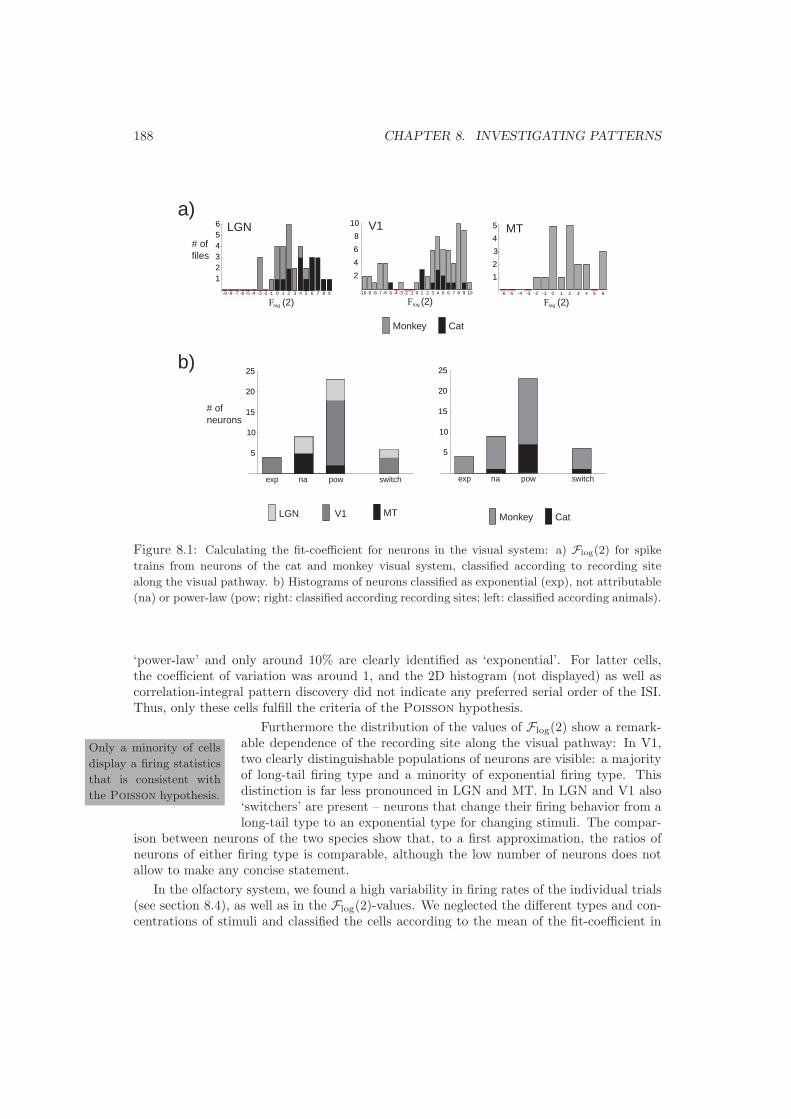
188 CHAPTER 8. INVESTIGATING PATTERNS
-9 -8 -7 -6 -5 -4 -3 -2 -1 0 1 2 3 4 5 6 7 8 9
123456
-10 -9 -8 -7 -6 -5 -4 -3 -2 -1 0 1 2 3 4 5 6 7 8 9 10
2
4
6
8
10
-6 -5 -4 -3 -2 -1 0 1 2 3 4 5 6
1
2
3
4
5LGN V1 MT# of files
CatMonkey
# of neurons
CatMonkey
a)
b)
F (2)log F (2)log F (2)log
5
10
15
20
25
V1LGN MT
exp na pow switch
5
10
15
20
25
exp na pow switch
Figure 8.1: Calculating the fit-coefficient for neurons in the visual system: a) Flog(2) for spike
trains from neurons of the cat and monkey visual system, classified according to recording site
along the visual pathway. b) Histograms of neurons classified as exponential (exp), not attributable
(na) or power-law (pow; right: classified according recording sites; left: classified according animals).
‘power-law’ and only around 10% are clearly identified as ‘exponential’. For latter cells,the coefficient of variation was around 1, and the 2D histogram (not displayed) as well ascorrelation-integral pattern discovery did not indicate any preferred serial order of the ISI.Thus, only these cells fulfill the criteria of the Poisson hypothesis.
Only a minority of cells
display a firing statistics
that is consistent with
the Poisson hypothesis.
Furthermore the distribution of the values of Flog(2) show a remark-able dependence of the recording site along the visual pathway: In V1,two clearly distinguishable populations of neurons are visible: a majorityof long-tail firing type and a minority of exponential firing type. Thisdistinction is far less pronounced in LGN and MT. In LGN and V1 also‘switchers’ are present – neurons that change their firing behavior from along-tail type to an exponential type for changing stimuli. The compar-
ison between neurons of the two species show that, to a first approximation, the ratios ofneurons of either firing type is comparable, although the low number of neurons does notallow to make any concise statement.
In the olfactory system, we found a high variability in firing rates of the individual trials(see section 8.4), as well as in the Flog(2)-values. We neglected the different types and con-centrations of stimuli and classified the cells according to the mean of the fit-coefficient in
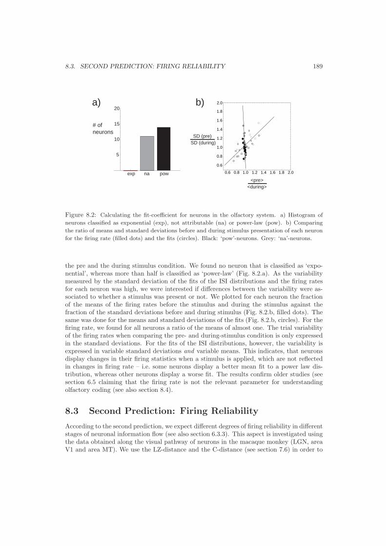
8.3. SECOND PREDICTION: FIRING RELIABILITY 189
0.6 0.8 1.0 1.2 1.4 1.6 1.8 2.0
0.6
0.8
1.0
1.2
1.4
1.6
1.8
2.0
<pre><during>
SD (pre)SD (during)
exp na pow
5
10
15
20a) b)
# ofneurons
Figure 8.2: Calculating the fit-coefficient for neurons in the olfactory system. a) Histogram of
neurons classified as exponential (exp), not attributable (na) or power-law (pow). b) Comparing
the ratio of means and standard deviations before and during stimulus presentation of each neuron
for the firing rate (filled dots) and the fits (circles). Black: ‘pow’-neurons. Grey: ‘na’-neurons.
the pre and the during stimulus condition. We found no neuron that is classified as ‘expo-nential’, whereas more than half is classified as ‘power-law’ (Fig. 8.2.a). As the variabilitymeasured by the standard deviation of the fits of the ISI distributions and the firing ratesfor each neuron was high, we were interested if differences between the variability were as-sociated to whether a stimulus was present or not. We plotted for each neuron the fractionof the means of the firing rates before the stimulus and during the stimulus against thefraction of the standard deviations before and during stimulus (Fig. 8.2.b, filled dots). Thesame was done for the means and standard deviations of the fits (Fig. 8.2.b, circles). For thefiring rate, we found for all neurons a ratio of the means of almost one. The trial variabilityof the firing rates when comparing the pre- and during-stimulus condition is only expressedin the standard deviations. For the fits of the ISI distributions, however, the variability isexpressed in variable standard deviations and variable means. This indicates, that neuronsdisplay changes in their firing statistics when a stimulus is applied, which are not reflectedin changes in firing rate – i.e. some neurons display a better mean fit to a power law dis-tribution, whereas other neurons display a worse fit. The results confirm older studies (seesection 6.5 claiming that the firing rate is not the relevant parameter for understandingolfactory coding (see also section 8.4).
8.3 Second Prediction: Firing Reliability
According to the second prediction, we expect different degrees of firing reliability in differentstages of neuronal information flow (see also section 6.3.3). This aspect is investigated usingthe data obtained along the visual pathway of neurons in the macaque monkey (LGN, areaV1 and area MT). We use the LZ-distance and the C-distance (see section 7.6) in order to

190 CHAPTER 8. INVESTIGATING PATTERNS
5 10 15 20 25 30 35 40
0.2
0.4
0.6
0.8
1.0
200 400 600 800 1000
0.2
0.4
0.6
0.8
1.0
00
Firing rate [spikes/sec]
Dis
tanc
e
LZ-distance C-distance
a) b)
Dis
tanc
e
Firing rate [spikes/sec]
Figure 8.3: Relation between the C/LZ-distances and the firing rate for Poisson spike trains: a)
Small firing rates. b) Asymptotic behavior for large firing rates.
investigate firing reliability in terms of the mean distance between a set of spike trains ofone neuron obtained under equal stimulus conditions. The LZ-distance measures reliabilityin terms of similar firing patterns, whereas the C-distance indicates the similarity of firingin terms of spike timing.
Methods: We use recordings of 9 LGN neurons, 10 complex neurons in V1, 6 simpleneurons in V1 and 7 neurons in area MT as described in section 8.1.3. For the LGN-cells, 6-7 stimulus conditions have been evaluated. However, only 2-3 trials per stimulushave been performed. This limits the significance of the results obtained for this classof cells. For the V1 cells, 10 trials have been taken per cell and per stimulus (5orientations). For the MT cells, 6 trials have been taken (16 orientations). For eachset of spike trains emerging from trials performed on a specific cell and using a specificstimulus, the mean C- and LZ-distance between the trains have been calculated (thestandard deviation of the Gaussian kernel of the C-distance was 1 ms).
We expect an interrelation between the mean rate and the mean distance for each setof spike trains, because a higher firing rate increases the chance of coincident spikes andleads to smaller mean C-distances just because the rate is higher. We use the followingapproach to compare the reliability of neuronal firing independently of the firing rate.It is well-known that the most random distribution of events in time is provided by aPoisson process. Mean distances obtained by analyzing real data of a specific neuroncan then be compared with mean distances of a set of Poisson spike trains withsimilar rate. The larger the deviation, the more reliable (in terms of the distance used)fires this neuron. To investigate this aspect in more detail, we generated by meansof a Poisson process in total 72 classes of 10 spike trains each (duration: 10 secondsper train) with mean firing rates ranging from 0 spikes/second to 1000 spikes/secondsampled with a resolution of 1 ms. The majority of the trains had (physiologically

8.3. SECOND PREDICTION: FIRING RELIABILITY 191
meaningful) firing rates of 1-100 spikes/second. To analyze the limit behavior, alsohigher firing rates were used. For each class, the mean C- and LZ-distance have beencalculated (Fig. 8.3). For the C-distance we see that it is basically linearly related tothe firing rate for small rates and that it asymptotically approaches d(t, t∗) 0 forlarge firing rates. This is plausible, as the probability that the convolved trains overlapscales linearly with the increase in number of (randomly distributed) spikes for smallfiring rates and saturates asymptotically for large firing rates. By testing several fit-functions (polynomials, exponential and power-law functions) we found that a fourthorder polynomial of the type f(x) = ax4 + bx3 + cx2 + dx + e provided the best fitin terms of minimized mean-square errors (for a firing rate of 0, the function has apoint of discontinuity, as the mean distance would be zero). This function is taken asthe Poisson reference for the C-distance. The relation between the LZ-distance andthe firing rate is more complex. For small firing rates (up to ∼10 spikes/second) wefind a steady increase of the mean distances up to ∼0.2, which is followed by a veryslow increase for larger firing rates until ∼500 spikes/second. For larger firing rates,we find a symmetry along the vertical axis x = 500, which is plausible, because in thebit-coded spike trains basically a switch between the letters ‘0’ and ‘1’ is observed asthe spike train predominately consists of spikes. Again, several fit-functions have beentested. We obtained the best fit by using a fourth-order polynomial for the interval[0,20] spikes/second and a quadratic function for the interval [20,980] spikes/second.We use this composed function as the Poisson reference for the LZ-distance. Thedegree of discrepancy of the neuronal data to these two Poisson reference functions isour measure for the reliability of firing in terms of the C/LZ-distances. The discrepancyis measured as the average mean distance of all data points from these functions.
Four classes of reliabil-
ity: High for timing and
pattern (LGN), low for
timing and pattern (V1
complex), high or timing
and low for pattern (V1
simple), high for pattern
and low for timing (MT).
The results of the analysis of the four cell types investigated are dis-played in Fig. 8.4. Each point in the graph reflects the mean distanceof all trials of a single stimulus parameter (orientation) for a single neu-ron calculated using the LZ-distance (light grey) or the C-distance (darkgrey). The curves shown are the Poisson reference functions. We thendetermined the deviations of the mean distances of the trials from thePoisson reference for each distance measure and for each class of neu-rons in the different brain areas. As the standard deviations of the datasets obtained in this way (LGN, V1C, V1S, MT) were high, we pairwisetested the null-hypothesis that the two sets derive from the same dis-tribution using the non-parametric Wilcoxon-Mann-Whitney u-test withsignificance levels p < 0.05 and p < 0.001 (two-sided). The results are displayed in Fig. 6.For the C-distance, the data sets obtained from the MT-cells and the V1 complex cells arenot distinguished for p < 0.05 and p < 0.001, whereas the other sets are indeed recognizedas distinct distributions. For the LZ-distance and a significance level of p < 0.05, the datasets V1C and V1S, as well as V1S and LGN are not distinguished, but MT was classifiedas distinct. For the higher significance level p < 0.001, the data sets V1C, V1S, and LGN,as well as LGN and MT were not distinct. Taken together, the results suggest the followinginterpretation: In terms of the ‘timing deviation’ of the data from the Poisson reference,the V1 simple cells have the highest value, i.e. have the highest timing reliability, followedby the LGN cells and the MT/V1 complex cells. In terms of the ‘pattern deviation’ ofthe data from the Poisson reference, the MT neurons have the highest value, i.e. have thehighest ‘pattern reliability’, followed by the LGN, V1 simple and complex cells. Thus, the

192 CHAPTER 8. INVESTIGATING PATTERNS
0 40 80 1200.0
0.2
0.4
0.6
0.8
1.0
0 40 80 1200.0
0.2
0.4
0.6
0.8
1.0
0 40 80 1200.0
0.2
0.4
0.6
0.8
1.0
0 40 80 1200.0
0.2
0.4
0.6
0.8
1.0LGN
V1S
V1C
MT
Firing rate [spikes/sec]
Dis
tanc
e
LZ-distance C-distance
0.02 0.04 0.06 0.08 0.1
0.05
0.1
0.15
0.2
0.25
LGN
V1S
V1C
MT
V1S
LGN
MT
V1C
LGNV1SV1C MT
LGNV1SV1C MT
0
t < 0.001
t < 0.001
t < 0.05
a) b)Mean deviation from Poisson
using the LZ-distance
Mea
n de
viat
ion
from
Poi
sson
usin
g th
e C
-dis
tanc
e
Figure 8.4: Firing reliability determination of visual neurons: a) Relation between the C/LZ-
distances and the firing rate for spike trains obtained from neurons of areas LGN, V1 (comples:
V1C, and simple: V1S), and MT in macaque monkey. b) Timing and Pattern deviation from the
Poisson reference of neurons measured in areas LGN, V1 (complex/simple cells) and MT.
complex cells are closest to the Poisson model in both respects, whereas the MT cells havea considerable ‘pattern reliability’ and the V1 simple cells a considerable ‘timing reliability’.The LGN cells display both characteristics up to some degree, although we have to remindthat the number of trials per stimulus conditions in this case is low and requires a carefulinterpretation.
8.4 Third Prediction: Neuronal Clustering
We investigate the third prediction by analyzing the functional clustering within a neu-ronal network of an olfactory sensor when confronted by a specific odor. We address thisquestion using the LZ-distance and the C-distance as population criteria and the sequentialsuperparamagnetic clustering paradigm.
Methods: We use the LZ- and C-distance measure and the sequential superpara-magnetic clustering algorithm as explained in sections 7.6 and 7.5 on the completeolfactory data set described in section 8.1.1. The clustering parameters have been cho-sen as follows: minsize = 2 and sθ = 0.04. For the C-distance, spike trains that share alarge number of synchronous spikes are considered to be close. Therefore, the measurereflects the criterion of synchronization in neuronal group formation. As the intertrial-variability in the data set was high, and the number of trials per stimulus was low, we

8.4. THIRD PREDICTION: NEURONAL CLUSTERING 193
focussed our analysis on differences between the pre-stimulus and the during-stimuluscondition of the neuronal network, disregarding the identity and concentration of theapplied odors. The analysis has been performed in a three-step procedure: First, wedetermined the number of clusters of neurons in each of the 96 periods of recording,using both the LZ-distance and the C-distance. Second, based on this result, the meanand the standard deviation of the number of clusters across trials for both conditionswas calculated. For each neuron we then determined the mean size of the clusters towhich it belonged in the activity in the pre-stimulus period, and in the during-stimulusperiod. Periods of recording were excluded if no clusters formed. Such periods occurredin all four odors as well as in the pre- and during-stimulus period using both distancemeasures (LZ-distance: 11 times / C-distance: 18 times). Third, to quantify the inter-actions of each neuron with each other neuron in the during-stimulus period comparedto the pre-stimulus period, we assigned to each neuron a vector, whose componentsindicate the number of times the specified neuron finds itself in a cluster with anotherneuron. For example, for the i-th neuron, the vector has the form ni = (x1, . . . , x54),where xj indicates the number of times the i-th neuron is in the same group as thej -th neuron. The distance between two such vectors ni and nj is simply
d(ni, nj) = 1 − ni · nj
‖ni‖‖nj‖Using this measure, the proximity of two neurons indicates that they often partic-
ipate in the same cluster. Clustering with this distance measure works out the degreeof interrelation of neurons within the network, averaged over all trials (‘clusters amongpartners’). We determined the dendrogram for sθ = 0.02 such that also clusters oflow stability are detected. Based on the dendrogram showing the breakdown in clus-ters for decreasing cluster stability s, we identified the values of s, where new clustersemerged. The result (the dependence of the number of clusters on a required stabilitys) is displayed in diagrams for the pre- and during-stimulus condition. The diagramsindicate the ’stability behavior’ of the network in terms of the mean stability of in-terrelationships between neurons expressed via the LZ-distance or the C-distance. Ifthere are many clusters for high values of s, then the interrelatedness of the neuronsin the network is stable. Note, that in this analysis two different kinds of clusters areinvestigated. In the first step, the resulting clusters reflect the degree of relatedness ina single period of recording. In the third step, the resulting clusters reflect the meandegree of relatedness between the neurons of the network over all stimulus conditions.
Stable neuron clusters
signal odor presentation.
We first estimate the intertrial-variability of single cell firing by usinga moderate criterion, the change in firing rate over a coarse time scale.We calculated the firing rate vector of each spike train by partitioning thespike train in 10 ms segments and calculating the firing rate (spikes/sec)in each segment. The vectors obtained in this way reflect the change infiring rate of each spike train. For each neuron, the distances between all 96 firing ratevectors have been obtained by calculating the pairwise dot product. The resulting distancematrix has been used as input for the clustering algorithm. In neither case did clustersemerge, demonstrating that even when the same odor was applied in the same concentration,the intertrial-variability in firing rate was too high and prevented the formation of clustersin the three periods of activity recorded under matched stimulus conditions. For someneurons, we directly calculated the coefficient of variation in the average firing rate for spiketrains obtained unter matched stimulus conditions. In the large majority, the coefficient

194 CHAPTER 8. INVESTIGATING PATTERNS
c)
Odor1 Odor2 Odor3 Odor4 All files
2
4
6
8
10
# ofclusters
0
0.2 0.4 0.6 0.8
5
10
15
20
25
# ofclusters
Cluster stability s
0
d)
2
4
6
8
10
12
14
Odor1 Odor2 Odor3 Odor4 All files
# ofclusters
During-stimulusPre-stimulus
a)
0.2 0.4 0.6 0.8
5
10
15
20
25
# ofclusters
0
b)
Cluster stability s
0
LZ-distance C-distance
Figure 8.5: Olfactory neural network clustering, measured by the LZ-distance (left) and the C-
distance: a/c) Number of clusters in the pre- and during-stimulus condition. b/d) Stability of
‘clusters among partners’ (see text).
lay between 0.5-1.5, further indicating high intertrial-variability. This high variability inthe network requires an approach that compares the mean behavior of the network in thepresence or absence of an odor. It also confirms that, in this data, the firing rate of theindividual neuron is not an adequate means for understanding olfactory coding.
We performed the procedure described in the methods section using the LZ-distance asa similarity measure for clustering. The result of our analysis is shown in Fig. 8.5.a/b: Wefind that the number of clusters emerging on stimulus presentation does not per se indicatewhether the network is in a pre-stimulus or a during-stimulus condition. Also odor identitycannot be determined in this way. The large standard deviations reflect the intertrial-variability of the network behavior (Fig. 8.5.a/c). The analysis of the stability-behavior ofthe network (Fig. 8.5.b) provides new insight: the number of stable clusters (large values ofs) is lower in the pre-stimulus condition than in the during-stimulus condition; the numberof unstable clusters (small s) tends to be larger for a given s in the pre-stimulus conditionwhen compared with the during-stimulus condition. For s = 0.54, four clusters emerge inthe during-stimulus condition. This number increases to seven until an abrupt increase inthe number of clusters occurs at s = 0.08 . In the pre-stimulus condition we observe a single

8.5. FOURTH PREDICTION: CLASSES OF FIRING 195
cluster. Here, an even more abrupt increase in number sets in at s = 0.12. We performedthe same analysis using the C-distance for clustering. In this way, we focus on groups ofsynchronously firing neurons. As in the previous case, the number of pre- or during-stimulusclusters provide no information per se about stimulus presence or absence (Fig. 8.5.c). Thisresult is rather surprising, as the emergence of synchronization is considered as a possibleindicator for the presence of an odor. In this data, however, this seems not to be the case.The analysis of the stability behavior of the network shows that there is greater similaritybetween pre- and during-stimulus activity when considered in terms of synchronization ofthe network than when considered in terms of the LZ-distance (Fig. 8.5.d). Although aslightly higher degree of cluster stability is visible in the during-stimulus condition than forthe pre-stimulus condition (6 clusters emerge for s = 0.32 compared to s = 0.22 for thepre-stimulus condition), the effect is much less pronounced compared to that in the caseof the LZ-distance. This again indicates that synchronization effects in network behaviordo not necessarily reflect stimulus onset. In summary, our electrode array recordings fromthe olfactory bulb (mitral cell layer) of the rat reveal that stable inter-neuron relationships,expressed by the LZ-distance, emerge during odor presentation, and that these relationshipsare more stable than the synchronization of the neurons. These clusters reflect stimulus-evoked stabilization of the network-dynamics as expected by our hypothesis.
8.5 Fourth Prediction: Classes of Firing
Earlier investigations (see section 6.6.4) suggest the existence of three classes of neuronalfiring [429, 705]. According to our fourth prediction (section 6.6.5), we expect to reproducethis finding when analyzing the extended data set.
Methods: We apply the correlation integral based pattern discovery method as de-scribed in section 7.3 to our data set. We restrict ourselves to the data obtained in thevisual system, because the spike trains are generally much longer than those obtainedfrom the olfactory system and thus lead to statistically more reliable results (45 filesof LGN, 157 files of area V1 and 35 files of area MT). Eight files with a very smallnumber of ISI have been excluded from the analysis. The spike trains were embeddedin dimensions m = 1, . . . , 10. To distinguish steps in the log-log plot that emerged asa result of different length scales (which disappear for Poisson randomization) fromsteps that emerge from repeating sequences, we randomly shuffled the ISI of each trainand re-applied the correlation integral algorithm to the shuffled data. Each file has beenclassified according to the classes described in section 6.6.4. The most often representedclass in all five trials of a neuron determined, to which class the neuron belongs. Ineight neurons we found files, where different stimulus conditions led to a classificationinto groups I or III respectively. These cells were excluded from the analysis.
Three classes of neuronal
firing are also found in
the extended data set.
We found in all areas of the visual system of cat and monkey fromwhich data was available files and neurons of all three classes (fig. 8.6) Thefirst and the third class are more or less equal in size, whereas the secondclass is usually smaller. The analysis of the shuffled files (not displayed)showed that the majority of files that are categorized into classes I, II orIII remain in the same class after shuffling, indicating that the steps resultfrom pronounced differences in lengths scales and not from repeating sequences. However,

196 CHAPTER 8. INVESTIGATING PATTERNS
5
10
15
20
20
40
60
80
5
10
15
20
5
10
15
20
25
5
10
15
20
25
class I class II class III
LGN
class I class II class III
V1
class I class II class III
MT
class I class II class III class I class II class III
CatMonkey
CatMonkey
V1LGN MT
# of neurons
# of files
a)
b)
Figure 8.6: Pattern discovery in visual neuron spike trains: a) Number of files classified as I, II or
III in each visual area. b) number of neurons in each class, subdivided according to visual area and
species.
differences between the areas are visible: In LGN, none of the 45 files was classified inanother class after shuffling. In V1, 20 of 149 files that were classified in classes III or II fellafter shuffling in the classes II or I. In area MT, 4 of 35 files were re-classified after shuffling.This indicates, that interval patterns of l > 1 are present in at least some files in highercortical areas. As the number of neurons that we investigated is still rather limited, we cannot make any decisive statement about the relative sizes of each class in the several areasof the brain investigated. Furthermore, the stimulus used was in most cases not optimal forour analysis: neurons (V simple cells and some LGN neurons) that reproduce in their firingthe temporal structure of the stimulus (drifting gratings) certainly show two different lengthscales in the resulting spike trains – which again shows up as steps in the log-log plot. Toavoid this problem, more and different types of stimuli (as in the cat data) should have beenused. Unfortunately, we did not have access to this type of data.
8.6 Fifth Prediction: Pattern Stability
We apply our definition of pattern stability on data obtained from two complex V1 cells ofmacaque monkey. Both cells show a sharp peak at ∼100 Hz in the power spectrum (notdisplayed) that indicates oscillatory firing. The shift predictor indicates, that the oscillationof one neuron (neuron A) is driven by an external stimulus (possibly the frame rate of 100

8.6. FIFTH PREDICTION: PATTERN STABILITY 197
500
50
-
500
50
500
50
500
50
58 %16 %
81 %6 %
25 %35 %
29 %43 %
a)
b)
x i +1
x i +1
x i x i
0.05
0.1
0.15
0.2
0.25
0.05
0.1
0.15
0.2
SP SP
c) Periodicity 1 Periodicity 2
Neuron A
Neuron B
Neuron A
Neuron B
File 1 File 2
File 1 File 2
file 1
file 1
file 2
file 2
Figure 8.7: Pattern stability: a) 2D histogram of driven neuronal oscillator (neuron A). b) 2D
histogram of intrinsic neuronal oscillator (neuron B). c) Stability of all cells of the periodicity-1
oscillatory pattern for different matching intervals [−b, b] (right) and the stability of the periodicity-2
oscillatory pattern for optimal matching intervals (left).
Hz of the monitor on which the stimulus has been presented), whereas the second neuron(neuron B) is an intrinsic oscillator. We are interested, whether we find differences in thestability of the patterns associated with oscillatory firing.
Methods: We apply the definition of pattern stability of section 6.1.3. For patternquantification, we use a template-based approach as described in section 7.4 (no ad-ditional spikes were allowed within a sequence). To identify the template sequenceand the matching intervals adjusted to the individual noise levels of the files, we usesequential superparamagnetic clustering as described in section 7.5. For the clustering

198 CHAPTER 8. INVESTIGATING PATTERNS
algorithm, the parameters were set as: minsize: 25 and sθ: 5. We applied the cluster-ing algorithm to two files per neuron, where the most stablest clusters have been found.All files had large, stable clusters of points of the type (a, a), and smaller clusters of thetype (a, b) and (b, a) (a, b indicate ISI of different length scales). This indicates, that thefiring of both neurons is characterized by a firing of two periodicities: a periodicity-1firing – indicated by a pattern of the type a, a, a, a, . . . – and a periodicity-2 firing– indicated by a pattern of the type a, b, a, b, . . .. The noise affecting the firing ofneurons A and B, respectively, was different. In neuron A, the standard deviation ofthe coordinates of the stable clusters was in the order of 3 ms, whereas in neuron B,the standard deviation was in the order of 1 ms for the smaller coordinate and 2 ms forthe larger coordinate. This shows that the firing of neuron A is noisier as the firing ofneuron B, which is also clearly visible in the 2D histogram (Fig. 8.7.a/b). Therefore,for the template algorithm, the following sequences were investigated. For periodicity-1firing of cell A, the template had the form 9, 9, 9, . . . with matching interval [−3, 3]and for cell B, the template sequence was the same but the matching interval was[−2, 2]. To test the influence of the matching interval on the result, we also appliedthe algorithm to the files of A with matching interval [−2, 2] and to the ones of Bwith [−3, 3]. The result (not shown) shows that the matching interval suggested byclustering lead to the higher values in either case. This supports our claim, that theclustering algorithm provides optimal value for constructing the template sequence andthe matching interval.
The intrinsic periodicity-
2 pattern is much stabler
than the driven one.
After calculating the stability of the patterns associated with firing ofperiodicity-1 and periodicity-2 for both files of each neuron, we find nodifference of pattern stability for periodicity-1 firing between the drivenand the intrinsic neuronal oscillator (Fig. 8.7.c right). For neuron B(intrinsic oscillator) the stability values obtained for both files are com-parable (around 0.1), whereas for the driven oscillator, the stability values
of the two files are rather different (005 to 0.15). For periodicity-2 firing, a different pic-ture emerged. Here, the template algorithm was applied to the two files of cell A usingtemplate sequences of the form 9, 19, 9, 19, 9, . . . with matching intervals [−3, 3] for bothlength scales as suggested by the result of clustering. For the files of cell B, the templatesequence had the form 9, 2, 9, 2, 9, . . . with matching intervals [−2, 2] for the larger, and[−1, 1] for the smaller length scale (as suggested by clustering). Here (Fig. 8.7.c left), theintrinsic oscillator shows a three times more stable firing pattern of periodicity 2 than thedriven oscillator. The periodicity-2 firing of the intrinsic oscillator (cell B) is therefore amore stable phenomenon, as one would expect it in the framework of the Stoop-hypothesis,where higher periodicities may emerge as a result of a computation.

Chapter 9
Conclusions
In this chapter, we summarize the main achievements of the scientific part of the
thesis: We show to what extend the results of the previous chapter support the
Stoop-hypothesis, we put this result in the general context of neural coding and
computation, and include the more specific points on spike patterns, noise and
their functional role. We finalize this chapter by outlining possible experiments in
order to approach the open questions.
9.1 Support for the Stoop-Hypothesis
We have shown in the previous chapter that our predictions formulated in section 6.6.5 havebeen confirmed, although the available data were not optimal in all cases:
• The analysis of the ISI distributions demonstrated that the Poisson hypothesis doesnot cope with the majority of the data we investigated. The number of ‘Poisson neu-rons’ – i.e. neurons that are compatible with all conditions for claiming the validity ofthe Poisson hypothesis – was indeed surprisingly small. This finding is, however, notnecessarily contradicting the prediction of the Stoop-hypothesis that a considerablenumber of ‘noisy neurons’ (class I neurons) should be present, as class I neurons mustnot necessarily display a distinct Poisson firing statistics. When comparing the resultof the ISI distribution analysis with the result of correlation integral pattern discov-ery, we find that neurons classified as ‘not attributable’ often also fall into class I.Furthermore, the analysis of the firing statistics revealed a certain dependence on thefiring statistics from the stimulus. In the visual system, we found neurons classified as‘switcher’ – neurons that display exponential or long-tail firing statistics for differentstimulus conditions. In the olfactory system, we found a stimulus-related change of thefiring statistic variability. Both findings may be further analyzed when better data areavailable. We have to remind that, in the olfactory system, the spike trains availablefor calculating the distribution were rather short. In the visual system, on the otherhand, almost all files analyzed emanate from evoked and not from spontaneously activeneurons. Although non of the few files of spontaneous activity that were available to us
199

200 CHAPTER 9. CONCLUSIONS
were classified as exponential, it would be advantageous to include spontaneous spiketrains into the analysis, since many older studies on this matter based their findingson both spontaneous and evoked firing. Finally, the data that were available for uswere not sampled in order to obtain a representative set of neurons in respect to firingstatistics. Our result therefore do not allow a quantitative estimation of the sizes of thepopulations of exponential-firing or long-tail-firing neurons. It would be advantageousto have data that emerge from experiments with a broader class of stimuli.
• The analysis of firing reliability in the different visual areas also confirmed our ex-pectation that the reliability in respect of timing and patterns depends on whetherthe neuron acts more as a ‘information transmitter’ or as a ‘information processer’.Some aspects need, however, a careful interpretation. Our measure of reliability isbased on the deviation from a Poisson reference. Using the LZ-distance, the meandistance of some spike trains obtained in multiple presentations of a single stimuluscondition is higher than the Poisson reference – especially in area MT. Thus, theneurons may deviate from the reference function not in the sense that certain specificfiring patterns are replicated in the different trials, but that different firing patternsare present in different trials of a single stimulus condition. This interpretation maybe explained within the framework of the Stoop-hypothesis, as we expect that highercortical areas, where different types of computation may take place – as area MT –,display different types of patterns, whose actual presence and weighting in differenttrials of a single stimulus condition may change in the in vivo condition. This type offiring would, however, be well distinguished from Poisson firing.
• The result obtained by clustering of olfactory spike trains offers a promising approachfor analyzing the behavior of large neuronal networks, as it introduces an alterna-tive approach for studying neuronal population coding in the olfactory system. Wefound that stabilization of neural firing patterns, rather than synchronization, mayfaithfully represent an odor. This stabilization of the network can be interpreted asfollows: in prestimulus activity, the network is in a state with many unstable clus-ters. The network is thus in a ’preparatory state’ such that many potential neuronalgroups are available for encoding a given stimulus. During stimulus presentation, sta-ble clusters emerge out of these ’potential’ clusters, possibly representing the odor.This type of behavior is much less apparent using the C-distance, indicating that theeffect of synchronization is of less importance than might be theoretically predictedfor understanding population coding in the vertebrate olfactory system. This effect ofstabilization of a pattern is compatible with the Stoop-hypothesis, because we expectan increased computation during a stimulus. This is expressed in more stable patternthat lead to more stable clusters when the LZ-distance is used for clustering. Furtherstudies should focus on the question, whether clusters of spike trains can be related tospecific stimuli. This would need more trials per stimulus condition to cope with thelarge inter-trial variability.
• Our pattern discovery results basically confirmed the existence of the three firingclasses predicted by the Stoop-hypothesis. The classification obtained by analyzingthe monkey data was, however, more difficult to achieve as we found more ‘borderline’
9.2. THE STOOP-HYPOTHESIS IN THE GENERAL CONTEXT 201
cases. This might result from the fact that the set of stimuli used for obtaining themonkey data was more uniform as compared to the cat data.
• The concept of pattern stability was only applied to files of two neurons. We considerthis analysis as a preliminary test for the concept of pattern stability. It may be usedin experiments, where we can separate between patterns emerging from temporal cuesof the stimulus and pattern emerging as a result of a computational process. We hadcreated an experimental protocol on this matter,1 but were unable to find investigatorsthat could perform the necessary experiments.
9.2 The Stoop-Hypothesis in the General Context
The Stoop-hypothesis unifies several seemingly contradictory concepts in neural coding:Although the generic scheme of neuronal locking is based on neuron-neuron interaction, thegeneral framework emphasizes the role of groups of neurons. The hypothesis combines arate coding perspective (which provides the driving of a neuron) with a temporal codingperspective (the perturbation of the limit cycle and the emergence of a phase-locked firingbehavior). It attributes a precise role for the most important component of neuronal noisein the in vivo condition, the background activity, within neuronal information processing. Itfinally provides an alternative, dynamical systems based approach for understanding neuralcoding and neural computation. Based on a reconstruction of a system and a state spacepartition, the dynamics of neurons is encoded in state sequences that can be a further ob-ject of an analysis, using e.g. the Stoop-measure for computation. Results demonstratethat the computation improves when a neuron changes from a sub-optimal to an optimalstimulus [695]. Most of the discussed theoretical proposals concerning neural coding andneural computation – the synfire chain model, coincidence detection, and spike-timing de-pendent plasticity – can be related to the Stoop-hypothesis. Synfire chains, for example,might reliably transmit perturbation signals (synchronous spikes) to remote cortical areas.Coincidence detection provides us with a means to control the coupling parameter K bychanging the number of coincident spikes and thus the perturbation strength. Also spiketiming dependent plasticity might in principle be a way to change K. However, the chancesin synaptic strength induced by LTP or LTD are rather small and we therefore suggestthat spike timing dependent plasticity should be seen as a statistical effect changing manysynapses and thus the driving of of a neuron – or, in other words, the parameter Ω. Thetemporal correlation hypothesis in the sense of Singer et al., however, is not integrated inour framework, as we consider the binding of features as a result of locking expressed in theperiodicity of a spike train. In this way, we avoid a discussion on the several controversialaspects of the temporal correlation hypothesis.
9.3 Outlook: Experimental Approaches
Several constraints limited the empirical investigation of the prediction of the Stoop-hypothesis. The funding of the project did not allow to perform own experiments and the
1Markus Christen: Spike patterns in neuronal information processing – an experimental setup, 2003(working paper)

202 CHAPTER 9. CONCLUSIONS
available data were not in all respect optimal for the questions we are interested in. There-fore, there is still a need for an empirical underpinning of central claims of the hypothesis.The main open questions are:
• To what physical limits extends locking? This includes the testing of biological per-turbation profiles like different kinds of burst patterns, of the generic locking scheme(Fig. 6.7) with other neurons than pyramidal neurons in vitro and of the generallocking scheme in vivo. Furthermore, the highest possible perturbation frequenciesat which the locking phenomenon is still observable should be determined in in vitroexperiments.
• Can locking persist under dynamic network activity? This includes the test in vivothat locking remains under homogeneously changed activity, the determination of thesmallest input that triggers observable locking, and the determination of the dynamicrange that is applicable without loss of locking. Finally, inhomogeneous changes shouldresult in changing periodicities, which again should be observable in the in vitro con-dition, where the inhomogeneous change can be controlled by the experimentator. Asalready indicated in section 6.6, model studies demonstrate that locking persists alsounder changing driving conditions [698, 699]. This suggests that experiments in thisrespect lead to results in favor of the Stoop-hypothesis.
• What is the physiological background of the three classes of firing we postulated?One must find a clear reason how class I neurons are able to erase timing cues in thestimulus (for example provided by drifting gratings or the frame rate) and produce anoutput that only correlates with a general activity level.
• The integral framework presented by us can serve as a paradigm for large scale neuralmodelling using simple types of neurons, where the two basic types (class I and classIII) are implemented and connected according Fig. 6.11. Within this scheme, also theeffect of LTP as a means to increase the driving of limit cycle firing could be tested.Furthermore, recent work2 focusses the connection between architecture and compu-tation within neuronal networks. The results indicate that a fractal and recurrentnetwork architecture is optimal for information speed and computation (measured ac-cording to Ref. [695]). These promising results are object of a follow-up PhD studyby Stefan Martignoli.
In this work, we have clarified the term ‘spike pattern’, discussed the problem of patterndetection and we have introduced novel methods for solving this problem. We furthermorehave shown, how the Stoop-hypothesis is related to the current discussion on neural codingand neural computation, why the Stoop-hypothesis is interesting, and that the data avail-able to us support prediction of this hypothesis. We believe that the tests outlined abovewould help to further understand and complete the hypothesis and exploit its potential forobtaining a deeper understanding of the information processing brain.
2A diploma thesis performed by Stefan Martignoli in 2005, as well as ongoing work that is currentlysubmitted or in preparation (C Wagner & R Stoop: Neocortex’s small world of fractal coupling / C Wagner& R Stoop: Neocortex’s architecture optimizes synchronization and information propagation under a totalconnection length constraint. / S. Martignoli & R Stoop: Cortical recurrent connections maximize a measureof computation).

Part III
Appendix
203


List of Figures
1.1 Scheme of argumentation . . . . . . . . . . . . . . . . . . . . . . . . . . . . . 4
2.1 Shannon’s scheme of a communication system . . . . . . . . . . . . . . . . . 172.2 Scheme for historical analysis: before transition . . . . . . . . . . . . . . . . . 222.3 The emergence of the spike . . . . . . . . . . . . . . . . . . . . . . . . . . . . 292.4 The emergence of the spike train . . . . . . . . . . . . . . . . . . . . . . . . . 30
3.1 Scheme for historical analysis: after transition . . . . . . . . . . . . . . . . . . 323.2 Examples of network-structures from early neural modelling studies . . . . . 54
4.1 The neuroscience boom since the Second World War . . . . . . . . . . . . . . 674.2 Journal analysis . . . . . . . . . . . . . . . . . . . . . . . . . . . . . . . . . . . 684.3 Cluster analysis of conferences . . . . . . . . . . . . . . . . . . . . . . . . . . 734.4 Identifying important conferences . . . . . . . . . . . . . . . . . . . . . . . . . 744.5 Citation analysis for McCulloch . . . . . . . . . . . . . . . . . . . . . . . . 814.6 Citation analysis for Gerard . . . . . . . . . . . . . . . . . . . . . . . . . . . 824.7 Citation analysis for Barlow . . . . . . . . . . . . . . . . . . . . . . . . . . . 834.8 Citation analysis for Bullock . . . . . . . . . . . . . . . . . . . . . . . . . . 844.9 Citation analysis for MacKay . . . . . . . . . . . . . . . . . . . . . . . . . . 854.10 Citation analysis for Reichardt . . . . . . . . . . . . . . . . . . . . . . . . . 864.11 Overview historical developments . . . . . . . . . . . . . . . . . . . . . . . . . 87
5.1 The dimensions of a code relation . . . . . . . . . . . . . . . . . . . . . . . . . 975.2 Representations of spike trains . . . . . . . . . . . . . . . . . . . . . . . . . . 98
6.1 Types of spike patterns . . . . . . . . . . . . . . . . . . . . . . . . . . . . . . 1096.2 The stability of an interval pattern . . . . . . . . . . . . . . . . . . . . . . . . 1116.3 Methods of randomization . . . . . . . . . . . . . . . . . . . . . . . . . . . . . 1176.4 The degree of randomization introduced by shuffling procedures . . . . . . . . 1186.5 Neuronal noise sources . . . . . . . . . . . . . . . . . . . . . . . . . . . . . . . 1206.6 Limit cycle firing . . . . . . . . . . . . . . . . . . . . . . . . . . . . . . . . . . 1396.7 Locking and Arnol’d coding . . . . . . . . . . . . . . . . . . . . . . . . . . . 1416.8 The coding problem in the framework of dynamical systems theory . . . . . . 1426.9 Arnol’d coding in the (Ω,K) parameter space . . . . . . . . . . . . . . . . . 1456.10 Classes of neuronal firing . . . . . . . . . . . . . . . . . . . . . . . . . . . . . 148
205
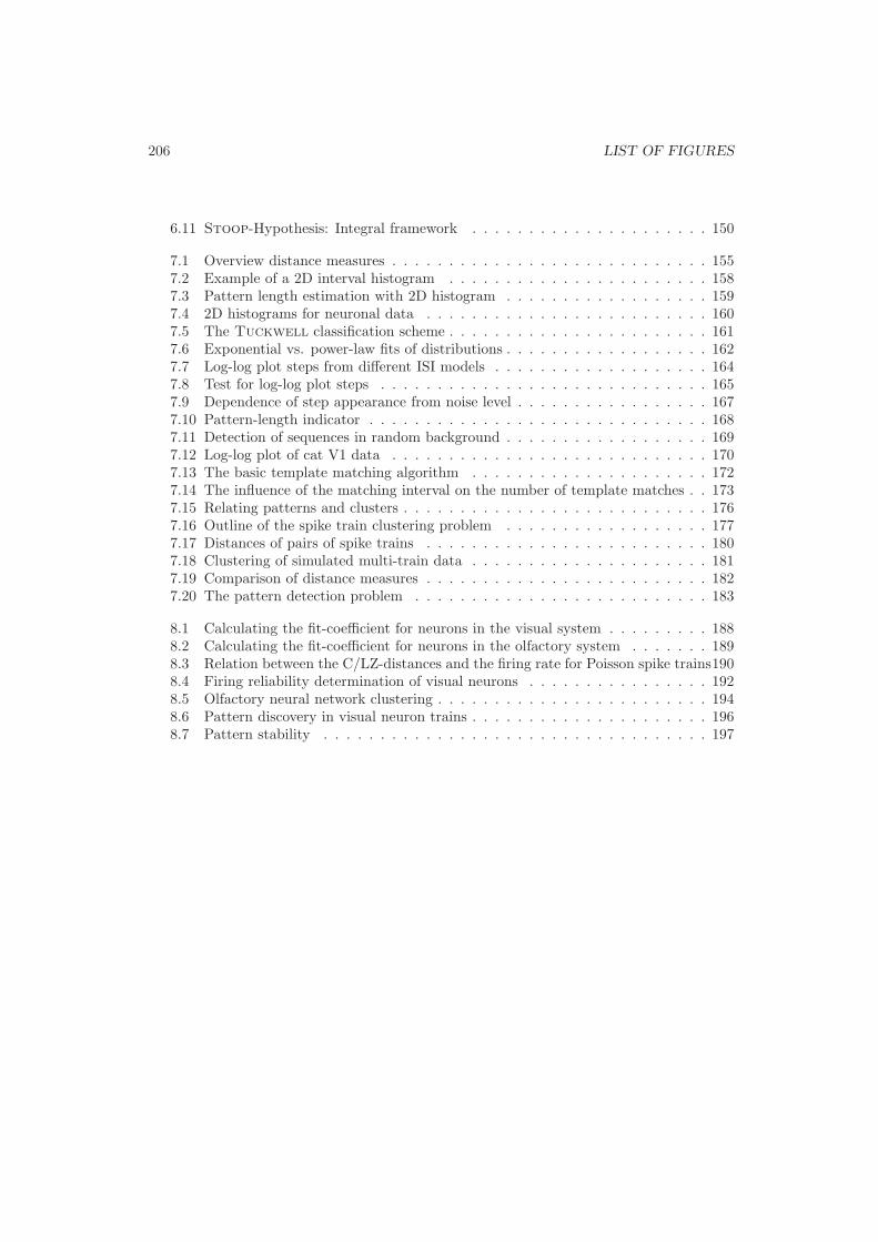
206 LIST OF FIGURES
6.11 Stoop-Hypothesis: Integral framework . . . . . . . . . . . . . . . . . . . . . 150
7.1 Overview distance measures . . . . . . . . . . . . . . . . . . . . . . . . . . . . 1557.2 Example of a 2D interval histogram . . . . . . . . . . . . . . . . . . . . . . . 1587.3 Pattern length estimation with 2D histogram . . . . . . . . . . . . . . . . . . 1597.4 2D histograms for neuronal data . . . . . . . . . . . . . . . . . . . . . . . . . 1607.5 The Tuckwell classification scheme . . . . . . . . . . . . . . . . . . . . . . . 1617.6 Exponential vs. power-law fits of distributions . . . . . . . . . . . . . . . . . . 1627.7 Log-log plot steps from different ISI models . . . . . . . . . . . . . . . . . . . 1647.8 Test for log-log plot steps . . . . . . . . . . . . . . . . . . . . . . . . . . . . . 1657.9 Dependence of step appearance from noise level . . . . . . . . . . . . . . . . . 1677.10 Pattern-length indicator . . . . . . . . . . . . . . . . . . . . . . . . . . . . . . 1687.11 Detection of sequences in random background . . . . . . . . . . . . . . . . . . 1697.12 Log-log plot of cat V1 data . . . . . . . . . . . . . . . . . . . . . . . . . . . . 1707.13 The basic template matching algorithm . . . . . . . . . . . . . . . . . . . . . 1727.14 The influence of the matching interval on the number of template matches . . 1737.15 Relating patterns and clusters . . . . . . . . . . . . . . . . . . . . . . . . . . . 1767.16 Outline of the spike train clustering problem . . . . . . . . . . . . . . . . . . 1777.17 Distances of pairs of spike trains . . . . . . . . . . . . . . . . . . . . . . . . . 1807.18 Clustering of simulated multi-train data . . . . . . . . . . . . . . . . . . . . . 1817.19 Comparison of distance measures . . . . . . . . . . . . . . . . . . . . . . . . . 1827.20 The pattern detection problem . . . . . . . . . . . . . . . . . . . . . . . . . . 183
8.1 Calculating the fit-coefficient for neurons in the visual system . . . . . . . . . 1888.2 Calculating the fit-coefficient for neurons in the olfactory system . . . . . . . 1898.3 Relation between the C/LZ-distances and the firing rate for Poisson spike trains1908.4 Firing reliability determination of visual neurons . . . . . . . . . . . . . . . . 1928.5 Olfactory neural network clustering . . . . . . . . . . . . . . . . . . . . . . . . 1948.6 Pattern discovery in visual neuron trains . . . . . . . . . . . . . . . . . . . . . 1968.7 Pattern stability . . . . . . . . . . . . . . . . . . . . . . . . . . . . . . . . . . 197

List of Tables
4.1 Conferences of the Macy-cluster . . . . . . . . . . . . . . . . . . . . . . . . . . 694.2 Work sessions and ISP of the NRP-cluster . . . . . . . . . . . . . . . . . . . . 704.3 Theory-Cluster . . . . . . . . . . . . . . . . . . . . . . . . . . . . . . . . . . . 724.4 Biology cluster . . . . . . . . . . . . . . . . . . . . . . . . . . . . . . . . . . . 724.5 Border crossers . . . . . . . . . . . . . . . . . . . . . . . . . . . . . . . . . . . 774.6 Ambassadors . . . . . . . . . . . . . . . . . . . . . . . . . . . . . . . . . . . . 774.7 ‘Important people’ of American origin . . . . . . . . . . . . . . . . . . . . . . 784.8 ‘Important people’, emigrants to the US . . . . . . . . . . . . . . . . . . . . . 784.9 ‘Important people’, non-Americans . . . . . . . . . . . . . . . . . . . . . . . . 79
7.1 Overview histograms . . . . . . . . . . . . . . . . . . . . . . . . . . . . . . . . 1577.2 Maximum number of steps s(l,m) . . . . . . . . . . . . . . . . . . . . . . . . 1667.3 Slope ratio determination . . . . . . . . . . . . . . . . . . . . . . . . . . . . . 168
8.1 Overview data set . . . . . . . . . . . . . . . . . . . . . . . . . . . . . . . . . 186
207

208 LIST OF TABLES

Bibliography
[1] Historical Sources (up to ∼1980)[2] Abeles M, and MH Goldstein (1977): Multispike train analysis. Proceedings of the IEEE 65(5): 762-
773.
[3] Abeles M, and Y Lass (1975): Transmission of information by the axon: II the channel capacity.Biological Cybernetics 19: 121-125.
[4] Adrian ED (1947): The physical background of perception. Clarendon Press, Oxford.
[5] Adrian ED, and G Moruzzi (1939): Impulses in the pyramidal tract. Journal of Physiology 97: 153-199.
[6] Adrian ED (1932): The mechanism of nervous action. University of Pennsylvania Press, Philadelphia.
[7] Adrian ED (1930): The effect of injury on mammalian nerve fibres. Proceedings of the Royal Societyof London B 106: 596-618.
[8] Adrian ED (1928): The basis of sensation. Christophers, London.
[9] Adrian ED (1926): The impulses produced by sensory nerve endings. Part I. Journal of Physiology61: 49-72.
[10] Adrian ED, and Y Zotterman (1926): The impulses produced by sensory nerve-endings. Part 2. Theresponse of a single end-organ. Journal of Physiology 61: 151-171.
[11] Adrian ED, and Y Zotterman (1926): The impluse produced by sensory nerve endings. Part 3. Impulsesset up by touch and pressure. Journal of Physiology 61: 465-483.
[12] Aitkin LM, CW Dunlop, and WR Webster (1966): Click-evoked response patterns of single units inthe medial geniculate body of the cat. Journal of Neurophysiology 29(1): 109-123.
[13] Amassian VE, J Macy Jr., HJ Waller, HS Leader, and M Swift (1964): Transformation of afferentactivity at the cuneate nucleus. In: RW Gerard, and JW Duyff: Information processing in the nervoussystem. Excerpta Medica Foundation, Amsterdam, New York: 235-254.
[14] Arbib MA (1972): The metaphorical brain. An introduction to cybernetics as artificial intelligenceand brain theory. John Wiley & Sons Inc., New York.
[15] Arbib MA (1969): Automata theory as an abstract boundary condition for the study of informationprocessing in the nervous system. In: KN Leibovic: Information processing in the nervous system.Springer Verlag, Berlin, Heidelberg, New York: 3-19.
[16] Arnol’d IV (1965): Small denominators I, Mappings of the circumference onto itself. Transactions ofthe American Mathematical Society (Series 2) 46: 213-284.
[17] Ashby WR (1966): Mathematical models and computer analysis of the function of the central nervoussystem. Annual Review of Physiology 28: 89-106.
[18] Ashby WR, H von Foerster, and CC Walker (1962): Instability of pulse activity in a net with threshold,Nature 196: 561-562.
[19] Ashby, WR (1952): Design for a brain. John Wiley & Sons Inc., New York.
[20] Ashby WR (1950): The stability of a randomly assembled nerve-network. Electroencephalography andClinical Neurophysiology 2(4): 471-482.
209
210 BIBLIOGRAPHY
[21] Atwood HL, and CAG Wiersma (1967): Command interneurons in the crayfish central nervous system.Journal of Experimental Biology 46: 249-261.
[22] Bar-Hillel Y, and R Carnap (1953): Semantic information. British Journal of the Philosophy of Science4: 147-157.
[23] Barlow HB (1972): Single units and sensation: a neuron doctrine for perceptual psychology? Percep-tion 1: 371-394. Reprinted in: JA Anderson, A Pellionisz, and E Rosenfeld (eds.): Neurocomputing2. Directions for research. MIT Press, Cambridge: 218-234.
[24] Barlow HB (1969): Trigger features, adaptation and economy. In: KN Leibovic (ed.): Informationprocessing in the nervous system. Springer Verlag, Berlin, Heidelberg, New York: 209-230.
[25] Barlow HB (1963): The information capacity of nervous transmission. Kybernetik 2(1): 1.
[26] Barlow HB (1961): Possible principles underlying the transformations of sensory messages. In: WARosenblith: Sensory Communication, MIT-Press, Cambridge: 217-234.
[27] Barlow HB (1961): The coding of sensory messages. In: WH Thorpe, and OL Zangwill (eds.): Currentproblems in animal behaviour. Cambridge University Press, Cambridge: 331-360.
[28] Barlow HB (1959): Sensory mechanisms, the reduction of redundancy, and intelligence. In: NationalPhysical Laboratory: Mechanisation of Thought-Processes, volumes I/II. London, Her Majesty’s Sta-tionery Office: 537-574.
[29] Barlow HB (1953): Summation and inhibition in the frog’s retina. Journal of Physiology 119: 69-88.
[30] Beurle RL (1956): Properties of a mass of cells capable of regenerating pulses. Philosophical Transac-tions of the Royal Society of London B 240(669): 55-94.
[31] Biscoe TJ, and A Taylor (1963): The discharge pattern recorded in chemoreceptor afferent fibresfrom the cat carotid body with normal circulation and during perfusion. Journal of Physiology 168:332-344.
[32] Bishop PO, WR Levick, and WO Williams (1964): Statistical analysis of the dark discharge of lateralgeniculate neurons. Journal of Physiology 170: 598-612.
[33] Bishop GH (1956): Natural history of the nerve impulse. Physiological Review 36: 376-399.
[34] Bishop GH, and M Clare (1953): Sequence of events in optic cortex response to volleys of impulses inthe radiation. Journal of Neurophysiology 16(5): 490-498.
[35] Blair EA, and J Erlanger (1935): On the process of excitation by brief shocks in axons. AmericanJournal of Physiology 114: 309-316.
[36] Blair EA, and J Erlanger (1933): A comparison of the characteristics of axons through their individualelectrical responses. American Journal of Physiology 106: 524-564.
[37] Blair EA, and J Erlanger (1932): Responses of axons to brief shocks. Proceedings of the Society ofexperimental Biology and Medicine 29: 926-927.
[38] Blaschko H, M Cattell, and JL Kahn (1931): On the nature of the two types of response in theneuromuscular system of the crustacean claw. Journal of Physiology 73: 25-35.
[39] Blum M (1962): Properties of a neuron with many inputs. In: H von Foerster, and W George:Principles of self-organization. Pergamon Press, New York: 95-119.
[40] Braitenberg V (1961): Functional interpretation of cerebellar histology. Nature 190: 539-540.
[41] Braitenberg V, G Gambardella, and U Vota (1965): Observation on spike sequences from sponta-neously active Purkinje cells in the frog. Kybernetik 2(5): 197-205.
[42] Brazier MA (1964): The biologist and the communication sciences. In: RW Gerard, and JW Duyff:Information processing in the nervous system. Excerpta Medica Foundation, Amsterdam, New York:87-94.
[43] Brazier MA (1963): How can models from information theory be used in neurophysiology? In: WSFields, and W Abbott (eds.): Information storage and neural control. Charles C. Thomas Publisher,Springfield, Illinois: 230-242.
[44] Brazier MA (1957): Rise of neurophysiology in the 19th century. Journal of Neurophysiology 20(2):212-226.

BIBLIOGRAPHY 211
[45] Brink F, DW Bronk and MG Larrabee (1946): Chemical excitation of nerve. Annals of the New YorkAcademy of Sciences, 47, 457-485, 1946.
[46] Bronk DW, and LK Ferguson (1934): The nervous control of intercostal respiration. American Journalof Physiology 110: 700-707.
[47] Brudno S, and TJ Marczynski (1977): Temporal patterns, their distribution and redundancy in trainsof spontaneous neuronal spike intervals of the feline hippocampus studied with a non-parametrictechnique. Brain Research 125: 65-89.
[48] Bryant HL, and JP Segundo (1976): Spike initiation by transmembrane current: A white noise analysis.Journal of Physiology 260: 279-314.
[49] Bullock TH (1970): The reliability of neurons. The Journal of General Physiology 55: 565-584.
[50] Bullock TH (1968): The Representation of information in neurons and sites for molecular participation.Proceedings of the National Academy of Science USA 60(4): 1058-1068.
[51] Bullock TH (1967): Signals and neuronal coding. In: GC Quarton, T Melnechuk, and FO Schmitt(eds.): The neurosciences. A study program. The Rockefeller University Press, New York: 347-352.
[52] Bullock TH, and GA Horridge (1965): Structure and function in the nervous systems of invertebrates,volume I. W.H. Freeman and Company, San Francisco, London.
[53] Bullock TH (1964): Transfer functions at synaptic junctions. In: RW Gerard, and JW Duyff (eds.):Information processing in the nervous system. Excerpta Medica Foundation, Amsterdam, New York:98-108.
[54] Bullock TH (1961): The origins of patterned nervous discharge. Behaviour 17: 48-59.
[55] Bullock TH (1959): Neuron doctrine and electrophysiology. Science 129: 997-1002.
[56] Burke RE, P Rudomin, and FE Zajac (1970): Catch properties in single mammalian motor units.Science 168: 122-124.
[57] Burns BD (1968): The uncertain nervous system. Edward Arnold Ltd., London.
[58] Burns BD, and GK Smith (1962): Transmission of information in the unaenesthetized cat’s isolatedforebrain. Journal of Physiology 164: 238-251.
[59] Burns BD (1958): The mammalian cerebral cortex. Edward Arnold Ltd., London.
[60] Caianiello ER (ed.) (1968): Neural networks. Proceedings of the school on neural networks. SpringerVerlag, Berlin, Heidelberg, New York.
[61] Caianiello ER (1964): Mathematical and physical problems in the study of brain models. In: RF Reiss:Neural theory and modeling. Stanford University Press, Stanford: 98-104.
[62] Caianiello ER (1961): Outline of a theory of thought-processes and thinking machines. Journal ofTheoretical Biology 2: 204-235.
[63] Calvin WH (1968): Evaluating membrane potential and spike patterns by experimenter-controlledcomputer display. Experimental Neurology 21: 512-534.
[64] Calvin WH, and CF Stevens (1968): Synaptic noise and other sources of randomness in motorneuroninterspike intervals. Journal of Neurophysiology 31(4): 574-587.
[65] Calvin WH, and CF Stevens (1967): Synaptic noise as a source of variability in the interval betweenaction potentials. Science 155: 842-844.
[66] Cherry C (ed.) (1956): Information Theory. Papers read at a symposium on ‘information theory’ heldat the Royal Institution. London, September 12th to 16th 1955. Butterworths Scientific Publications,London.
[67] Cherry C (ed.) (1961): Information Theory. Papers read at a symposium on ‘information theory’held at the Royal Institution, London, August 29th to September 2nd 1960. Butterworths ScientificPublications, London.
[68] Cowan JD (1968): Statistical mechanics of nervous nets. In: ER Caianiello: Neural networks. SpringerVerlag, Berlin, Heidelberg, New York: 181-188.

212 BIBLIOGRAPHY
[69] Cox DR, and PAW Lewis (1966): The statstical analysis of series of events. Methuen & Co Ltd.,London.
[70] Cox DR (1962): Renewal theory. Methuen & Co. Ltd., London.
[71] Derksen HE, and AA Verveen (1966): Fluctuations of resting neural membrane potential. Science 151:1388-1389.
[72] Douglas WW, JM Ritchie, and W Schaumann (1956): A study of the effect of the pattern of electricalstimulation of the aortic nerve on the reflex depressor responses. Journal of Physiology 133: 232-242.
[73] Ead HW, JH Green and E Neil (1952): A comparison of the effects of pulsative and non-pulsativeblood flow through the caroid sinus on the reflexogenic activity of the sinus baroreceptors in the cat.Journal of Physiology 118: 509-519.
[74] Eckhorn R, and B Popel (1974): Rigorous and extended application of information theory to theafferent visual system of the cat. I. Basic concepts. Kybernetik 16: 191-200.
[75] Emmers R (1976): Thalamic mechanisms that process a temporal pulse code for pain. Brain Research103: 425-441.
[76] Evarts EV (1964): Temporal patterns of discharge of pyramidal tract neurons during sleep and wakingin the monkey. Journal of Neurophysiology 27(2): 152-171.
[77] Farber G (1968): Berechnung und Messung des Informationsflusses der Nervenfaser. Kybernetik 5(1):17-29.
[78] Fatt P, and B Katz (1952): Spontaneous subthreshold activity at motor nerve endings. Journal ofPhysiology 117: 109-128.
[79] Fatt P, and B Katz (1950): Some observations on biological noise. Nature 166: 597-598.
[80] Fehmi LG, and TH Bullock (1967): Discrimination among temporal patterns of stimulation in acoomputer model of a coelenterate nerve net. Kybernetik 3(5): 240-249.
[81] Fields WS, and W Abbott (eds.) (1963): Information storage and neural control. Charles C. ThomasPublisher, Springfield, Illinois.
[82] Fisher RA (1925): Theory of statistical estimation. Proceedings of the Cambridge Philosophical Society22: 700-725.
[83] Fitch FB (1944): Review of: Warren S. McCulloch and Walter Pitts. A logical calculus of the ideasimmanent in the nervous activity. The Journal of Symbolic Logic 9(2): 49-50.
[84] FitzHugh R (1958): A statistical analyzer for optic nerve messages. The Journal of General Physiology41(4): 675-692.
[85] FitzHugh R (1956): The statistical detection of treshold signals in the retina. The Journal of GeneralPhysiology 40(6): 925-947.
[86] Forbes A, and C Thacher (1920): Amplification of action currents with the electron tube in recordingwith the string galvanometer. The American Journal of Physiology 52(3): 409-471.
[87] Forbes A, and A Gregg (1915): Electrical studies in mammalian reflexes. I. The flexion reflex. AmericanJournal of Physiology 37: 118-176.
[88] Gasser HS, and J Erlanger (1922): A study of the action currents of nerve with the athode rayoscillograph. American Journal of Physiology 62: 496-524.
[89] George FH (1961): The brain as a computer. Pergamon Press, Oxford.
[90] Gerard LB, JG Miller, and A Rapoport (1975): Ralph Waldo Gerard. Behavioral Science 20(1): 1-8.
[91] Gerard RW, and JW Duyff (eds.) (1964): Information processing in the nervous system. Proceed-ings of the International Union of Physiological Sciences, volume III. Excerpta Medica Foundation,Amsterdam, New York.
[92] Gerard RW (1951): Some of the problems concerning digital notions in the central nervous system.In: H von Foerster, M Mead, and HL Teuber: Cybernetics. Circular causal and feedback mechanismsin biological and social systems. Transactions of the seventh conference (March 23-24, 1950), NewYork : 11-57.

BIBLIOGRAPHY 213
[93] Gerstein GL, DH Perkel, and KN Subramanian (1978): Identification of functionally related neuralassemblies. Brain Research 140: 43-62.
[94] Gerstein GL, and DH Perkel (1972): Mutual temporal relationship among neuronal spike trains.Biophysical Journal 12: 453-473.
[95] Gerstein GL (1960): Analysis of firing patterns in single neurons. Science, 131, 1811-1812, 1960.
[96] Gerstein GL, and NY-S Kiang (1960): An approach to the quantitative analysis of electrophysiologicaldata from single neurons. Biophysical Journal 1: 15-28.
[97] Gerstein GL, and B Mandelbrot (1964): Random walk models for the spike activity of a single neuron.Biophysical Journal 4: 41-68.
[98] Gerstein GL, and WA Clark (1964): Simultaneous studies of firing patterns in several neurons. Science143: 1325-1327.
[99] Gerstein GL, and DH Perkel. Simultaneously recorded trains of action potentials: Analysis and func-tional interpretation. Science 164, 828-830, 1969.
[100] Gillary HL, and D Kennedy (1969): Neuromuscular effects of impulse pattern in a crustacean Mo-toneuron. Journal of Neurophysiology 32: 607-612.
[101] Gillary HL, and D Kennedy (1969): Pattern generation in a crustacean motoneuron. Journal ofNeurophysiology 32: 595-606.
[102] Glaser EM, DS Ruchkin (1976): Principles of neurobiological signal analysis. New York, San Francisco,London. Academic Press.
[103] Goldstein K (1934): Der Aufbau des Organismus. Martinus Nijhoff, Den Haag.
[104] Goldstine HH (1961): Information theory. Science 133: 1395-1399.
[105] Gregory RL (1961): The brain as an engineering problem. In: WH Thorpe, and OL Zangwill (eds.):Current problems in animal behaviour. Cambridge University Press, Cambridge: 307-330.
[106] Griffith JS (1971): Mathematical neurobiology. Academic Press, London, New York.
[107] Griffith JS (1963): On the stability of brain-like structures. Biophysical Journal 3: 299-308.
[108] Grossman RG, and LJ Viernstein (1961): Discharge patterns of neurons in cochlear nucleus. Science134: 99-101.
[109] Grusser, O-J, KA Hellner, and U Grusser-Cornehls (1962): Die Informationsubertragung im afferentenvisuellen System. Kybernetik 1(5): 13-192.
[110] Grusser O-J (1962): Die Informationskapazitat einzelner Nervenzellen fr die Signalubermittlung imZentralnervensystem. Kybernetik 1(5): 209-211.
[111] Grundfest H (1957): Excitations at synapses. Journal of Neurophysiology 20(3): 316-327.
[112] Hagiwara S, and H Morita (1963): Coding mechanisms of electroreceptor fibers in some electric fish.Journal of Neurophysiology 26: 551-567.
[113] Hagiwara S (1954): Analysis of interval fluctuation of the sensory nerve impulse. Japanese Journal ofPhysiology 4: 234-240.
[114] Harmon LD, and ER Lewis (1966): Neural Modeling. Physiological Review 46: 513-591.
[115] Harmon LD (1964): Problems in neural modeling. In: RF Reiss: Neural theory and modeling. StanfordUniversity Press, Stanford: 9-30.
[116] Hartley RVL (1928): Transmission of information. Bell System Technical Journal 7: 535-563.
[117] Hartline HK, CH Graham (1932): Nerve impulses from single receptors in the eye. Journal of Cellularand Comparative Physiology 1(2): 277-295.
[118] Hassenstein B (1960): Die bisherige Rolle der Kybernetik in der biologischen Forschung. III. Diegeschichtliche Entwicklung der biologischen Kybernetik bis 1948. Naturwissenschaftliche Rundschau11: 419-424.
[119] Hebb DO (1949/1961): The organization of behavior. A neuropsychological theory. John Wiley &Sons Inc., New York.

214 BIBLIOGRAPHY
[120] Herz AVM, O Creutzfeldt, and JM Fuster (1964): Statistische Eigenschaften der Neuronaktivitat imascendierenden visuellen System. Kybernetik 2(2): 61-71.
[121] Hind JE, JM Goldberg, DD Greenwood, and FE Rose (1963): Some discharge characteristics of singleneurons in the inferior colliculus of the cat. II Timing of the discharges and observations on binauralstimulation. Journal of Neurophysiology 26(4): 321-341.
[122] Hintikka J (1968): The varieties of information and scientific explanation. In: B Rootselaar, JF vander Staal: Logic, methodology and philosophy of science, vol. 3. Amsterdam: 311-331.
[123] Hodgkin AL, and AF Huxley (1939): Action potentials recorded from inside a nerve fibre. Nature 144:710-711.
[124] Householder AS, and HD Landahl (1945): Mathematical biophysics of the central nervous system.The Principia Press Inc., Bloomington, Indiana.
[125] Huygens C (1673): Horologium Oscillatorium. Muguet, Paris.
[126] Jacobson H (1951): The information capacity of the human eye. Science 113: 292-293.
[127] Jacobson H (1950): The information capacity of the huma ear. Science 112: 143-144.
[128] Jeffress LA (ed.) (1951): Cerebral mechanisms in behavior. The Hixon symposium. John Wiley &Sons, New York.
[129] Kalenich WA (ed.) (1966): Information processing 1965. Proceedings of the IFIP congress 65. SpartanBooks, Washington D.C.
[130] Katsuki Y, S Yoshino, and J Chen (1950): Action currents of the single lateral-line nerve fiber of fish.1. On the spontaneous discharge. Japanese Journal of Physiology 1: 87-99.
[131] Katz B, and R Miledi (1970): Membrane noise produced by acetylcholine. Nature 226: 962-963.
[132] Kenshalo DR (ed.) (1968): The skin senses. Proceedings of the first international symposium on theskin senses. Charles C. Thomas Publisher, Springfield, Illinois.
[133] Kolmogorov AN (1957): The theory of transmission of information. In: The session of the Academy ofSciences of the USSR on Scientific Problems of Industrial Automation, October 15-20 1956. Reprintedin: AN Shiryayev (ed.): Selected works of A.N. Kolmogorov, volume III: 6-30.
[134] Kolmogorov AN (1941): Interpolation und Extrapolation von stationaren zufalligen Folgen. Bulletinde l’academie des Sciences de l’Union des Republiques Sovjetiques Socialistes 5: 11-14.
[135] Kubie L (1930): A theoretical application to some neurological problems of the properties of excitationwaves which move in closed circuits. Brain 53: 166-177.
[136] Kuffler SW, R FitzHugh, and HB Barlow (1957): Maintained activity on the cat’s retina in light anddarkness. The Journal of General Physiology 40(5): 683-702.
[137] Landahl HD, W McCulloch, and W Pitts (1943): A statistical consequence of the logical calculus ofnervous nets. Bulletin of Mathematical Biophysics 5: 135-137.
[138] Landahl HD (1939): Contributions to the mathematical biophysics of the central nervous system.Bulletin of Mathematical Biophysics 1(2): 95-118.
[139] Lashley KS (1951): The problem of serial order in behavior. In: LA Jeffress (ed.): Cerebral mechanismsin behavior. John Wiley & Sons, New York: 112-146.
[140] Lashley KS (1933): Integrative functions of the cerebral cortex. Physiological Reviews 13(1): 1-42.
[141] Lashley KS (1931): Mass action in cerebral function. Science 73: 245-254.
[142] Leibovic KN (1969): Information processing in the nervous system. Springer Verlag, Berlin, Heidel-berg, New York.
[143] Lempel A, and Ziv J (1976): On the complexity of finite sequences. IEEE Transactions on InformationTheory IT-22: 75-81.
[144] Lewis RE (1968): The iron wire model of the neuron: A review. In: HL Oestreicher, and DR Moore:Cybernetic problems in bionics. Gordon and Breach Science Publishers Inc., New York, London, Paris:247-273.

BIBLIOGRAPHY 215
[145] Ling G, RW Gerard (1949): The normal membrane potential of frog sartorius fibers. Journal ofCellular and Comparative Physiology 34: 383-394.
[146] Lucas K (1917): The conduction of the nervous impulse. Longmans, Green and Co., London.
[147] MacKay DM (1966): Information in brains and machines. In: WA Kalenich (ed.): Information pro-cessing 65. Spartan Books, Washington: 637-643.
[148] MacKay DM (1956): The place of ‘meaning’ in the theory of information. In: C Cherry (ed.): Infor-mation theory. Butterworths Scientific Publications, London: 215-225.
[149] MacKay DM (1954): On comparing the brain with machines. American Scientist 42: 261-268.
[150] MacKay DM, and W McCulloch (1952): The limiting information capacity of a neuronal link. Bulletinof Mathematical Biophysics 14: 127-135.
[151] Martin AR, and C Branch (1958): Spontaneous activity of betz cells in cats with midbrain lesions.Journal of Neurophysiology 21: 368-379.
[152] Marczynski TJ, and CJ Sherry (1971): A new analysis of trains of increasing or decreasing interspikeintervals treated as self-adjusting sets of ratios. Brain Research 35: 533-538.
[153] McCulloch W (1965): Embodiments of mind. The MIT Press, Cambridge, Massachusetts.
[154] McCulloch W (1964): A historical introduction to the postulational foundations of experimental epis-temology. In: FSC Northrop and HH Livingston (eds.): Cross-cultural understanding: Epistemologyin antrhopology. Harper & Row Publishers Inc., New York. Reprinted in: W McCulloch: Embodimentsof mind: 359-372.
[155] McCulloch W (1960): The reliability of biological systems. In: MC Yovits, and S Cameron: Self-organizing systems. Pergamon Press, Oxford: 264-281.
[156] McCulloch W (1957): Biological computers. IRE Transactions on Electronic Computers, September:190-192.
[157] McCulloch W (1951): Why the mind is in the head. In: LA Jeffress (ed.): Cerebral mechanisms inbehavior. John Wiley & Sons, New York: 42-57.
[158] McCulloch W (1949): The brain as a computing machine. Electrical Engineering 68: 492-497.
[159] McCulloch W, and W Pitts (1943): A logical calculus of the ideas immanent in nervous activity.Bulletin of Mathematical Biophysics 5: 115-133.
[160] Melzack R, and PD Wall (1962): On the nature of cutaneous sensory mechanisms. Brain 85: 331-356.
[161] Milner PM (1974): A model for visual shape recognition. Psychological Review 81(6): 521-535.
[162] Monnier A-M, HH Jasper (1932): Recherche de la relation entre les potentiels d’action elementaires etla chronaxie subordination, nouvelle demonstration du fonctionnement par “tout ou rien” de la fibrenerveuse. Comptes rendus des sceances de la societe de biologie et ses filiales 110: 547-549.
[163] Moore GP, DH Perkel and JP Segundo. Statistical analysis and functional interpretation of neuronalspike data. Annual Review of Physiology, 28, 493-522, 1966.
[164] Mountcastle VB (1975): The view from within: Pathways to the study of perception. John Hopkinsmedical journal (supplement) 136: 109-131.
[165] Mountcastle VB (1967): The problem of sensing and the neural code of sensory events. In: GCQuarton, T Melnechuk, and FO Schmitt (eds.): The neurosciences. A study program. The RockefellerUniversity Press, New York: 393-408.
[166] Nachmansohn D, H Merritt (1954): Nerve Impulse. Josiah Macy Jr. Foundation, New York.
[167] Nachrichtentechnische Gesellschaft im VDE Fachausschuss ‘Informations- und Systemtheorie’ (Hg.)(1961): Aufnahme und Verarbeitung von Nachrichten durch Organismen. S. Hirzel, Stuttgart.
[168] Nakahama H, S Nishioka, T Otsuka, and S Aikawa (1966): Statistical dependence between interspikeintervals of spontaneous activity in thalamic lemniscal neurons. Journal of Neurophysiology 29(5):921-941.
[169] National Physical Laboratory (1959): Mechanisation of Thought-Processes, volumes I/II. London, HerMajesty’s Stationery Office.

216 BIBLIOGRAPHY
[170] Oestreicher HL, and DR Moore (eds.) (1968): Cybernetic problems in bionics. Gordon and BreachScience Publishers Inc., New York, London, Paris.
[171] Pattee HH (1974): Discrete and continuous processes in computers and brains. In: M Conrad, WGuttinger, and M Dal Cin (eds.): Physics and mathematics of the nervous system. Springer-Verlag,Berlin, Heidelberg, New York: 128-148.
[172] Pecher C (1939): La fluctuation d’excitabilite de la fibre nerveuse. Archives Internationales de Phys-iologie XLIX(2): 129-152.
[173] Pecher C (1937): Fluctuations independantes de l’exitabilite de deux fibres d’un meme nerf. Comptesrendus des sceances de la societe de biologie et ses filiales. 124: 839-842.
[174] Peirce CS (1906/1960): Prolegomena to an apology for pragmaticism. In: C Hartshorne, and P Weiss:Collected Papers of Charles Sanders Peirce, volume III/IV. Cambridge. The Belknap Press of HarvardUniversity Press: Paragraph 4.537.
[175] Perkel DH, GL Gerstein, MS Smith, and WG Tatton (1975): Nerve-impulse patterns: a quantitativedisplay technique for three neurons. Brain Research 100: 271-296.
[176] Perkel DH (1970): Spike trains as carriers of information. In: FO Schmitt (ed.): The Neurosciences.2. study program. The Rockefeller University Press, New York: 587-596.
[177] Perkel DH, and TH Bullock (1968): Neural Coding. Neuroscience Research Progress Bulletin 6(3):221-348.
[178] Perkel DH, GL Gerstein, and GP Moore (1967): Neural spike trains and stochastic point processes. I.The single spike train. Biophysical Journal 7: 391-418
[179] Perkel DH, GL Gerstein and GP Moore. Neuronal spike trains and stochastic point processes. IISimultaneous spike trains. Biophysical Journal, 7, 419-440, 1967.
[180] Pfaffenhuber E (1974): Sensory coding and economy of nerve impulses. In: M Conrad, W Guttinger,and M Dal Cin (eds.): Physics and mathematics of the nervous system. Springer Verlag, Berlin,Heidelberg, New York: 469-483.
[181] Pierce WH (1965): Failure-tolerant computer design. Academic Press, New York, London.
[182] Pinneo LR (1966): On noise in the nervous system. Psychological Review 73(3): 242-247.
[183] Poggio GF, and LJ Viernstein (1964): Time series analysis of impulse sequences of thalamic somaticsensory neurons. Journal of Neurophysiology 27(4): 517-545.
[184] Pribram K (1960): A review of theory in physiological psychology. Annual Review of Psychology 11:1-40,
[185] Pringle JWS, and VJ Wilson (1952): The response of a sense organ to a harmonic stimulus. Journalof Experimental Biology 29: 220-234.
[186] Province de Namur (1958): 1er congres international de cybernetique. Namur, AssociationInternationale de Cybernetique.
[187] Quarton GC, T Melnechuk, and FO Schmitt (eds.) (1967): The neurosciences. A study program. TheRockefeller University Press, New York.
[188] Quastler H (1958): A primer of information theory. In: HP Yockey, RL Platzman, and H Quastler(eds.): Symposium on information theory in biology. Pergamon press, London: 3-49.
[189] Quastler H (1958c): The status of information theory in biology. In: HP Yockey, RL Platzman, andH Quastler (eds.): Symposium on information theory in biology. Pergamon Press, London: 399-402.
[190] Quastler H (1957): The complexity of biological computers. IRE Transactions on Electronic Comput-ers, September: 192-194.
[191] H Quastler (ed.) (1953): Essays on the use of information theory in biology. University of IllinoisPress, Urbana.
[192] Rapoport A (1964): Information processing in the nervous system. In: RW Gerard, and JW Duyff(eds.): Information processing in the nervous system. Excerpta Medica Foundation, Amsterdam, NewYork: 16-23.
BIBLIOGRAPHY 217
[193] Rapoport A, and W Horvath (1960): The theoretical channel capacity of a single neuron as determinedby various coding systems. Information and Control 3: 335-350.
[194] Rapoport A, and A Shimbel (1948): Steady states in random nets: I. Bulletin of MathematicalBiophysics 10: 211-220.
[195] Rapoport A (1948): Steady states in random nets: II. Bulletin of Mathematical Biophysics 10: 221-226.
[196] Rashevsky N (1948): Mathematical Biophysics. The University of Chicago Press, Chicago.
[197] Rashevsky N (1946): The neural mechanism of logical thinking. Bulletin of Mathematical Biophysics8: 29-40.
[198] Reiss RF (ed.) (1964): Neural theory and modeling. Proceedings of the 1962 Ojai Symposium. StanfordUniversity Press, Stanford.
[199] Reiss RF (1964): A theory of resonant networks. In: RF Reiss (ed.): Neural theory and modeling.Stanford University Press, Stanford: 105-137.
[200] Ripley SH, and CAG Wiersma (1953): The effect of spaced stimulation of excitatory and inhibitoryaxons of the crayfish. Physiologia Comparata et Oecologia 3: 1-17.
[201] Rodieck RW, NY-S Kiang, and GL Gerstein (1962): Some quantitative methods for the study ofspontaneous activity of single neurons. Biophysical Journal 2: 351-368.
[202] Rose JE, JF Brugge, DJ Anderson, and JE Hind (1967): Phase-locked resonse to low-frequency tonesin single auditory nerve fibers of the squirrel monkey. Journal of Neurophysiology 30: 769-793.
[203] Rose JE, DD Greenwood, JM Goldberg, JE Hind (1963): Some discharge characteristics of singleneurons in the inferior colliculus of the cat. I. Tonotopical organization, relation of spike-count to toneintensity, and firing patters of single elements. Journal of Neurophysiology 26(2): 294-319.
[204] Rosenblatt F (1962): Principles of neurodynamics. Spartan Books, Washington D.C.
[205] Rosenblith WA (ed.) (1961): Sensory Communication, Contributions to the symposium on principlesof sensory communication. MIT Press, Cambridge and John Wiley & Sons,New York, London.
[206] Rosenblith WA (1959): Some quantifiable aspects of the electrical activity of the nervous system (withemphasis upon responses to sensory simuli). Reviews of Modern Physics 31(2): 532-545.
[207] Rosenblueth A, and N Wiener (1950): Purposeful and non-purposeful behavior. Philosophy of Science17: 318-326.
[208] Rosenblueth A, N Wiener, and J Bigelow (1943): Behavior, Purpose and Teleology. Philosophy ofScience 10: 18-24.
[209] Rudolfer SM, and HU May (1975): On the Markov properties of interspike times in the cat optic tract.Biological Cybernetics 19: 197-199.
[210] Saltzberg B (1963): What is information theory? In: WS Fields, and W Abbott(eds.): Informationstorage and neural control. Charles C. Thomas Publisher, Springfield, Illinois.
[211] Schiller PH, BL Finlay, and SF Volman (1976): Short-term resopnse variability of monkey striateneurons. Brain Research 105: 347-349.
[212] Schmitt FO, G Adelman, and FG Worden (eds.) (1977): Neurosciences research symposium sum-maries, volume 8. MIT Press, Cambridge, London.
[213] Schmitt FO, and F Worden (ed.) (1974): The neurosciences. Third study program. The MIT Press,Cambridge, London.
[214] Schmitt FO, G Adelman, and FG Worden (eds.) (1973): Neurosciences research symposium sum-maries, volume 7. MIT Press, Cambridge, London.
[215] Schmitt FO, G Adelman, T Melnechuk, and FG Worden (eds.) (1972): Neurosciences research sym-posium summaries, volume 6. MIT Press, Cambridge, London.
[216] Schmitt FO, G Adelman, T Melnechuk, and FG Worden (eds.) (1971): Neurosciences research sym-posium summaries, volume 5. MIT Press, Cambridge, London.

218 BIBLIOGRAPHY
[217] Schmitt FO (ed.) (1970): The neurosciences. Second study program. The Rockefeller University Press,New York.
[218] Schmitt FO, T Melnechuk, GC Quarton, and G Adelman (eds.) (1970): Neurosciences research sym-posium summaries, volume 4. MIT Press, Cambridge, London.
[219] Schmitt FO, T Melnechuk, GC Quarton, and G Adelman (eds.) (1969): Neurosciences research sym-posium summaries, volume 3. MIT Press, Cambridge, London.
[220] Schmitt FO, T Melnechuk, and GC Quarton (eds.) (1967): Neurosciences research symposium sum-maries, volume 2. MIT Press, Cambridge, London.
[221] Schmitt FO, and T Melnechuk (eds.) (1966): Neurosciences research symposium summaries, volume1. MIT Press, Cambridge, London.
[222] Segundo JP (1970): Communication and coding by nerve cells. In: FO Schmitt (ed.): The neuro-sciences. Second study program. The Rockefeller University Press, New York: 569-586.
[223] Segundo JP, DH Perkel, and GP Moore (1966): Spike probability in neurones: Influence of temporalstructure in the train of synaptic events. Kybernetik 3(2): 67-82.
[224] Segundo JP, GP Moore, LJ Stensaas, and TH Bullock (1963): Sensitivity of neurones in Aplysia totemporal patternof arriving inpulses. The Journal of Experimental Biology 40: 643-667.
[225] Shannon CE, and J McCarthy (eds.) (1956): Automata studies. Princeton University Press, Princeton,New Jersey.
[226] Shannon CE, and W Weaver (1949): The mathematial theory of communication. University of IllinoisPress, Urbana.
[227] Shannon CE (1948): A mathematical theory of communication. The Bell Systems Technical Journal27: 379-423. Reprinted with corrections.
[228] Sherrington CS (1940/1951): Man on his nature. Cambridge University Press, Cambridge.
[229] Sherrington CS (1906/1909) The integrative action of the nervous system. Constable and CompanyLdt., London.
[230] Sherry CJ, and TJ Marczynski (1972): A new analysis of neuronal interspike intervals based oninequality tests. International Journal of Neuroscience 3: 259-270.
[231] Shimbel A (1950): Contributions to the mathemathical biophysics of the central nervous system withspecial references to learning. Bulletin of Mathematical Biophysics 12: 241-275.
[232] Shimbel A, and A Rapoport (1948): A statistical approach to the theory of the central nervous system.Bulletin of Mathematical Biophysics 10: 41-55.
[233] Sholl DA, and AM Uttley (1953): Pattern discrimination and the visual cortex. Nature 171: 387-388.
[234] Smith DR, and GK Smith (1965): A statistical analysis of the continual activity of single corticalneurones in the cat unanaesthetized isolated forebrain. Biophysical Journal 5: 47-74.
[235] Snow CP (1959): The two cultures and the scientific revolution. Cambridge University Press, NewYork.
[236] Stark L, and JF Dickson (1966): Mathematical concepts of central nervous system function. In:FO Schmitt, and T Melnechuk (eds.): Neuroscience Research Symposium Summaries 1. MIT-Press,Cambridge: 109-178.
[237] Stein RB (1970): The role of spike trains in transmitting and distorting sensory signals. In: FO Schmitt(ed.): The neurosciences. Second study program. Rockefeller University Press, New York: 597-604.
[238] Stein RB (1967): The information capacity of nerve cells using a frequency code. Biophysical Journal7: 797-826.
[239] Stein RB (1967): Some models of neuronal variability. Biophysical Journal 7: 37-68.
[240] Stein RB (1965): A theoretical analysis of neuronal variability. Biophysical Journal 5: 173-194.
[241] Steinbuch K (1961): Automat und Mensch. Uber menschliche und maschinelle Intelligenz. SpringerVerlag, Berlin, Gottingen, Heidelberg.
[242] Strehler BL (1977): Time, cells, and aging. New York, San Francisco, London. Academic Press.

BIBLIOGRAPHY 219
[243] Strehler BL (1969): Information handling in the nervous system: An analogy to molecular-geneticcoder-decoder mechanisms. Perspectives in Biology and Medicine 12: 584-612.
[244] Szilard L (1929): Uber die Entropieverminderung in einem thermodynamischen System bei Eingriffenintelligenter Wesen. Zeitschrift fur Physik 53: 840-856.
[245] Taylor R (1950): Comments on a mechanistic conception of purposefulness. Philosophy of Science 17:310-317.
[246] Terzuolo CA (1970): Data transmission by spik trains. In: FO Schmitt (ed.): The neurosciences.Second study program. Rockefeller University Press, New York: 661-671.
[247] Tomko GJ, and DR Crapper (1974): Neuronal variability: non-stationary responses to identical visualstimuli. Brain Research 79: 405-418.
[248] Turing AM (1936): On computable numbers, with an application to the Entscheidungsproblem. Pro-ceedings of the London Mathematical Society 42(2): 230-265.
[249] Uttal WR (1973): The psychobiology of sensory coding. Harper and Row, New York.
[250] Uttal WR (1969): Emerging principles of sensory coding. Perspectives in Biology and Medicine 12:344-368.
[251] Uttal WR, and M Krissoff (1968): Response of the somesthetic system to patterned trains of electricalstimuli. In: DR Kenshalo (ed.): The skin senses. Charles C. Thomas Publisher, Springfield: 262-303.
[252] Uttal WR (1960): The three stimulus problem: A further comparison of neural and psychophysicalresponses in the somesthetic system. Journal of Comparative and Physiological Psychology 53(1):42-46.
[253] Uttal WR (1959): A comparison of neural and psychophysical responses in the somesthetic system.Journal of Comparative and Physiological Psychology 52: 485-490.
[254] Uttley AM (1954): The classification of signals in the nervous system. Electroencephalography andClinical Neurophysiology 6: 479-494.
[255] Verveen AA, and HE Derksen (1965): Fluctuations in membrane potential of axons and the problemof coding. Kybernetik 2(4): 152-160.
[256] Viernstein LJ, and RG Grossman (1961): Neural discharge patterns in the transmission of sensoryinformation. In: C Cherry: Information theory. Butterworth, London: 252-269.
[257] Von Foerster H, and GW Zopf (eds.) (1962): Principles of self-organization. International tracts incomputer science and technology and their applications, volume 9. Pergamon Press, New York.
[258] Von Foerster H (ed.) (1950): Cybernetics. Circular causal and feedback mechanisms in biological andsocial systems, transactions of the sixth conference (march 24-25, 1949). New York. Re-issued in C.Pias (2003).
[259] Von Foerster H, M Mead, and HL Teuber (eds.) (1951): Cybernetics. Circular causal and feedbackmechanisms in biological and social systems, transactions of the seventh conference (march 23-24,1959). New York. Re-issued in C. Pias (2003).
[260] Von Foerster H, M Mead, and HL Teuber (eds.): Cybernetics. Circular causal and feedback mechanismsin biological and social systems, transactions of the eigtht conference (march 15-16, 1951). New York.Re-issued in C. Pias (2003).
[261] Von Foerster H, M Mead, and HL Teuber (1952): A note by the editors. In: H von Foerster, M Mead,and HL Teuber (eds.): Cybernetics. Circular causal and feedback mechanisms in biological and socialsystems, transactions of the eigtht conference (march 15-16, 1951). New York: xi-xx.
[262] Von Foerster H, M Mead, and HL Teuber (eds.) (1953): Cybernetics. Circular causal and feedbackmechanisms in biological and social systems, transactions of the ninth conference (march 20-21, 1952).New York. Re-issued in C. Pias (2003).
[263] Von Foerster H, M Mead, and HL Teuber (eds.) (1954): Cybernetics. Circular causal and feedbackmechanisms in biological and social systems, transactions of the tenth conference (april 22-24, 1953).New York. Re-issued in C. Pias (2003).
[264] Von Monakow C (1914): Die Lokalisation im Grosshirn und der Abbau der Funktion durch kortikaleHerde. Verlag von J.F. Bergman, Wiesbaden.

220 BIBLIOGRAPHY
[265] Von Neumann J (1966): The theory of self-reproducing automata. Edited and completed by AWBurcks. University of Illinois Press, Urbana.
[266] Von Neumann J (1958): The computer and the brain. Yale University Press, New Haven, London.
[267] Von Neumann J (1956): Probabilistic logics and the synthesis of reliable organisms from unreliablecomponents. In: CE Shannon, and J McCarthy (eds.): Automata studies. Princeton University Press,Princeton: 43-98.
[268] Von Neumann J (1951): The general and logical theory of automata. In: LA Jeffress (ed.): Cerebralmechanisms in behavior. John Wiley & Sons, New York: 1-41.
[269] Von Neumann J (1945/1993): First draft of a report on the EDVAC. Unpublished manuscript.Reprinted in: IEEE Annals of the History of Computing 15(4): 27-75.
[270] Wakabayashi T, and T Kuroda (1977): Effect of stimulation with impulse trains of various patterns,including adaptional type, on frog’s nerve-muscle and spinal reflex preparations. Tohoku Journal ofexperimental Medicine 121: 219-229.
[271] Wakabayashi T, and T Kuroda (1977): Responses of crayfish muscle preparations to nerve stimulationwith various patterns of impulse sequence. Effects of intermittent, intercalated and adaptational typesof impulse sequence. Tohoku Journal of experimental Medicine 121: 207-218.
[272] Walker AE (1957): Stimulation and Ablation. Their role in the history of cerebral physiology. Journalof Neurophysiology 20(4): 435-449.
[273] Wall PD, JY Lettvin, W McCulloch, and W Pitts (1956): Factors limiting the maximum impulsetransmitting ability of an afferent system of nerve fibres. In: C Cherry (ed.): Information Theory.Butterworths Scientific Publications, London: 329-344.
[274] Wayner MJ, and Y Oomura (1968): Meeting report: Neuronal Spike Trains. Science 160: 1025-1026.
[275] Weaver W (1948): Science and complexity. American Scientist 36: 536-544.
[276] Weddell G (1955): Somesthesis and the chemical senses. Annual Review of Psychology 6: 119-136.
[277] Whitsel BL, RC Schreiner, and GK Essick (1977): An analysis of variability in somatosensory corticalneuron discharge. Journal of Neurophysiology 40(3): 589-607.
[278] Wiener N (1949): Extrapolation, interpolation and smoothing of stationary time series. John Wiley& Sons Inc., New York.
[279] Wiener N (1949): Time, communication, and the nervous system. Annals of the New York Academyof Sciences 50(4): 197-220.
[280] Wiener N (1948): Cybernetics, or control and communication in the animal and the machine. MITPress, Cambridge.
[281] Wiersma CA, and RT Adams (1950): The influence of nerve impulse sequence on the contractions ofdifferent crustacean muscles. Physiologia Comparata et Oecologia 2: 20-33.
[282] Wilson DM, and JL Larimer (1968): The catch property of ordinar muscle. Proceedings of the NationalAcademy of Science USA 61: 909-916.
[283] Wilson DM, and WJ Davis (1965): Nerve impulse patterns and reflex control in the motor system ofthe crayfish claw. Journal of Experimental Biology 43: 193-210.
[284] Wilson DM, and RJ Wyman (1965): Motor output patterns during random and rhythmic stimulationof locust thoracic ganglia. Biophysical Journal 5: 121-143.
[285] Wilson DM (1964): The origin of the flight-motor command in grasshoppers. In: RF Reiss (ed.):Neural theory and modeling. Stanford University Press, Stanford: 331-345.
[286] Winograd S, and JD Cowan (1963): Reliable computation in the presence of noise. MIT ResearchMonograph, volume 2. MIT Press, Cambridge.
[287] Yockey HP, RL Platzman, and H Quastler (eds.) (1958): Symposium on information theory in biology.Pergamon Press, London.
[288] Young JZ (1964): A model of the brain. Clarendon Press, Oxford.

BIBLIOGRAPHY 221
[289] Yovits MC, and S Cameron (1960): Self-organizing systems. Proceedings of an interdisciplinary con-ference. Pergamon Press, Oxford, London.
[290] Zangwill OL (1961): Lashley’s concept of cerebral mass action. In: WH Thorpe, and OL Zangwill(eds.): Current problems in animal behavior. Cambridge University Press, Cambridge: 59-86.
[291] Ziv J, and A. Lempel (1978): Compression of individual sequences by variable rate coding. IEEETransactions on Information Theory IT-24: 530-536.
Secundary Literature[292] Abraham TH (2002): (Physio)logical circuits: The intellectual origins of the McCulloch-Pitts neural
network. Journal of the History of the Behavioral Sciences 38(1): 3-25.
[293] Adelman G, and BH Smith (eds.) (2004): Encyclopedia of neuroscience, third edition. Elsevier, Am-sterdam.
[294] Anderson JA, and E Rosenfeld (eds.) (1988): Neurocomputing. Foundations of research. MIT Press,Cambridge, London.
[295] Aspray W (1985): The scientific conceptualization of information: a survey. Annals of the History ofComputing 7(2): 117-140.
[296] Bennett MR, and PMS Hacker (2003): Philosophical foundations in neuroscience. Blackwell Publish-ing, Malden MA.
[297] Borck C (2002): Das elektrische Gehirn. Geschichte und Wissenskultur der Elektroenzephalographie.Habilitationsschrift, Institut fur Geschichte der Medizin, Freie Universitat Berlin. Erschienen 2005 als:Hirnstrome. Eine Kulturgeschichte der Elektroenzephalographie. Wallstein Verlag, Gottingen.
[298] Breidbach O (2001): The origin and development of the neurosciences. In: PK Machamer, R Grush,and P McLaughlin (eds.): Theory and method in the neurosciences. University of Pittsburgh Press,Pittsburgh: 7-29.
[299] Breidbach O (1997): Die Materialisierung des Ichs: Eine Geschichte der Hirnforschung im 19. und20. Jahrhundert. Suhrkamp Verlag, Frankfurt.
[300] Breidbach O (1995): From associative psychology to neuronal networks: The historical roots of Hebb’sconcept of the memory trace. In: N Elsner and R Menzel (eds.): Gottinger Neurobiologietagung 1995.Thieme Verlag, Stuttgart: 58.
[301] Breidbach O (1993): Nervenzellen oder Nervennetze? Zur Entstehung des Neuronenkonzeptes. In: EFlorey, and O Breidbach: Das Gehirn - Organ der Seele? City: Berlin Publisher: Akademie-VerlagPages: 81-126
[302] Bullock TH (1996: Theodore H. Bullock. In: LR Squire: The history of neuroscience in autobiography,volume 1. Society of Neuroscience, Washington D.C.
[303] Christen M (2006): Varieties of publication patterns in neuroscience at the cognitive turn. Journal ofthe History of the Neurosciences, submitted.
[304] Clarke E, and LS Jacyna (1987): Nineteenth century origins of neuroscientific concepts. University ofCalifornia Press, Berkeley.
[305] Cowan WM, DH Harter, and ER Kandel (2000): The emergence of modern neuroscience. Someimplications for neurology and psychiatry. Annual review of Neuroscience 23: 343-391.
[306] Dennett DC (1991): Real patterns. The Journal of Philosophy 88(1): 27-51.
[307] Dretske FI (1981/1999): Knowledge and the flow of information. MIT Press, Cambridge.
[308] Eco U (1972/2002): Einfuhrung in die Semiotik. Wilhelm Fink Verlag, Munchen..
[309] Fox Keller E (2002): Making sense of life. Explaining biological development with models, metaphors,and machines. Harvard University Press, Cambridge.
[310] Galison P (1994): The ontology of the enemy: Norbert Wiener and the cybernetic vision. CriticalInquiry 21: 228-266.
[311] Gardner HE (1985): The mind’s new science: A history of the cognitive revolution. Basic books, NewYork.
222 BIBLIOGRAPHY
[312] Garson J (2003): The introduction of information into neurobiology. Philosophy of Science 70: 926-936.
[313] Glanzel W, and U Schoepflin (1994): A stochastic model for the ageing of scientific literature. Scien-tometrics 30(1): 49-64.
[314] Godfrey MD, and DF Hendry (1993): The computer as von Neumann planned it. IEEE Annals of theHistory of Computing 15(1): 11-21.
[315] Grush R (2001): The semantic challenge to computational neuroscience. In: PK Machamer, R Grush,and P McLaughlin: Theory and method in the neurosciences. University of Pittsburgh Press, Pitts-burg: 155-172.
[316] Hagner M, and C Borck (2001): Mindful practices: on the neurosciences in the twentieth century.Science in Context 14(4): 507-510.
[317] Hagner M (1997/2000): Homo cerebralis: Der Wandel vom Seelenorgan zum Gehirn. Insel-Verlag,Frankfurt a.M.
[318] Hagner M (1993): Das Ende vom Seelenorgan. In: E Florey, and O Breidbach (eds.): Das Gehirn.Organ der Seele. Akademie Verlag, Berlin: 3-22.
[319] Hagner M (1999): Ecce Cortex. Beitrage zur Geschichte des modernen Gehirns. Wallstein Verlag,Gottingen.
[320] Hardcastle VG, C Stewart (2003): Neuroscience and the art of single cell recording. Biology andPhilosophy 18: 195-208.
[321] Hoah H (2003): Remote control. Nature 423: 796-799.
[322] Kay LE (2001): From logical neurons to poetic embodiments of mind: Warren S. McCulloch’s projectin neuroscience. Science in Context 14(4): 591-614.
[323] Kay LE (2000/2001): Who wrote the book if life? A history of the genetic code. Stanford UniversityPress, Stanford. German: Das Buch des Lebens. Wer schrieb den genetischen Code. Carl HanserVerlag, Munchen.
[324] Lettvin J (1999): McCulloch, Warren S. In: RA Wilson, and FC Keil: The MIT encyclopedia of thecognitive sciences. MIT press, Cambridge: 512-513.
[325] Lettvin J (1999): Pitts, Walter. In: RA Wilson, and FC Keil: The MIT encyclopedia of the cognitivesciences. MIT press, Cambridge: 651.
[326] Longuet-Higgins HC (1987): Donald MacKay (1922-1987). Nature 326: 446.
[327] Mendelsohn E, MR Smith, and P Weingart (eds.) (1988): Science, technology, and the military.Kluver, Dordrecht.
[328] Millman S (ed.) (1984): A history of engineering and science in the Bell system. CommunicationSciences (1925-1980). AT&T Bell Laboraties, Indianapolis.
[329] Muller A (2000): Eine kurze Geschichte des BCL. Osterreichische Zeitschrift fr Geschichtswis-senschaften 11 (1): 9-30.
[330] Oyama S (1985/2002): The ontogeny of information. Developmental systems and evolution. DukeUniversity Press, Durham.
[331] Penzlin H (2000): Die vergleichende Tierphysiologie In: I Jahn : Geschichte der Biologie. Spektrumakademischer Verlag, Heidelberg, Berlin: 461-498.
[332] Pias C (ed.) (2003): Cybernetics - Kybernetik. The Macy conferences 1946-1953. Transac-tions/Protokolle. Diaphanes Verlag, Zurich, Berlin.
[333] Pias C (ed.) (2004): Cybernetics - Kybernetik. The Macy conferences 1946-1953. Essays & documents/ Essays & Dokumente. Diaphanes Verlag, Zurich, Berlin.
[334] Pias C (2004): Zeit der Kybernetik – eine Einstimmung. In: Pias C (ed.) (2004): Cybernetics - Ky-bernetik. The Macy conferences 1946-1953. Essays & documents / Essays & Dokumente. DiaphanesVerlag, Zurich, Berlin: 9-41.
[335] Piccinini G (2004): The first computational theroy of mind and brain: A close look at McCulloch andPitt’s “Logical calculus of ideas immanent in nervous activity‘”. Synthese 141.2: 175-215.

BIBLIOGRAPHY 223
[336] Piccinini G (2004): Symbols, strings, and spikes. Unpublished manuscript, available under:http://artsci.wustl.edu/∼gpiccini
[337] Revonsuo A (2001): On the nature of explanation in neuroscience. In: PK Machamer, R Grush, andP McLaughlin: Theory and method in the neurosciences. University of Pittsburgh Press, Pittsburg:45-69.
[338] Schmiff FO (1992): The neurosciences research program: A brief history. In: F Samson, and GAdelman (eds.): The neurosciences: Paths of discovery II. Birkhauser Verlag, Boston, Basel, Berlin.
[339] Schnelle H (1976): Information. In: Historisches Worterbuch der Philosophie. Schwabe Verlag, Basel:356-357.
[340] Shepherd GM (1991): Foundations of the neuron doctrine. Oxford University Press, Oxford.
[341] Swazey JP (1975/1992): Forging a Neuroscience Community: A Brief History of the NeurosciencesResearch Program. In: FG Worden, JP Swazey, and G Adelman (eds.): The Neurosciences: Paths ofDiscovery, I. Birkhauser, Boston, Basel, Berlin.
[342] Szentagothai J (1975): From the last skirmishes around the neuron theory to the functional anatomy ofneuron networks. In: FG Worden, J Swazey, and G Adelman: The neurosciences – Paths of discovery.MIT Press, Cambridge: 103-120.
[343] Thagard P (2002): How molecules matter to mental computation. Philosophy of Science 69: 429-446.
[344] Williams MR (1993): The origins, uses and fate of the EDVAC. IEEE Annals of the History ofComputing 15(1): 22-38.
[345] Young RM (1970): Mind, brain, and adaption in the nineteenth century: Cerebral localization andits biological context from Gall to Ferrier. Clarendon Press, Oxford.
Scientific Literature (∼1980 – 2005)[346] Abbott LF, WG Regehr (2004): Synaptic computation. Nature 431: 796-803.
[347] Abbott LF (1994): Decoding neuronal firing and modelling neural networks. Quarterly Review ofBiophysics 27(3): 291-331.
[348] Abeles M, and I Gat (2001): Detecting precise firing sequences in experimental data. Journal ofNeuroscience Methods 107: 141-154.
[349] Abeles M, H Bergman, I Gat, I Meilijson, E Seidemann, and N Tishby (1995): Cortical activity flipsamong quasi-stationary states. Proceedings of the National Academy of Science USA 92: 8616-8620.
[350] Abeles M, Y Prut, H Bergman, and E Vaadia (1994): Synchronization in neuronal transmission andits importance for information processing. Progress in Brain Research 102: 395-404.
[351] Abeles M, H Bergman, E Margalit, and E Vaadia (1993): Spatiotemporal firing patterns in the frontalcortex of behaving monkeys. Journal of Neurophysiology 70(4): 1629-1638.
[352] Abeles M (1991): Corticonics. Neural circuits of the cerebral cortex. Cambridge University Press,Cambridge.
[353] Abeles M, and GL Gerstein (1988): Detecting spatiotemporal firing patterns among simultaneouslyrecorded single neurons. Journal of Neurophysiology 60(3): 909-924.
[354] Abeles M (1983): The quantification and graphic display of correlations among three spike trains.IEEE Transactions on Biomedical Engineering BME-30(4): 235-239.
[355] Abeles M, F de Ribaupierre, and Y de Ribaupierre (1983): Detection of single unit responses which areloosely time-locked to a stimulus. IEEE Transactions on Systems, Man, and Cybernetics SMC-13(5):683-691.
[356] Abeles M (1982): Quantification, smoothing, and confidence limits for single-units’ histograms. Journalof Neuroscience Methods 5: 317-325.
[357] Abeles M (1982): Role of the cortical neuron: Integrator or coincidence detector? Israel Journal ofMedical Sciences 18: 83-92.
[358] Abeles M (1982): Local cortical circuits. An electrophysiological study. Berlin, Heidelberg, New York,Springer.

224 BIBLIOGRAPHY
[359] Aertsen AMHJ, GL Gerstein, MK Habib, and G Palm (1989): Dynamics of neuronal firing correlation:Modulation of “effective connectivity”. Journal of Neurophysiology 61(5): 900-917.
[360] Ahmed B, JC Anderson, KAC Martin, and JC Nelson (1997): Map of the synapses onto layer 4 basketcell of the primary visual cortex of the cat. Journal of Computational Neuroscience 380(2): 230-242.
[361] Allen C, and CF Stevens (1994): An evaluation for causes for unreliability of synaptic transmission.Proceedings of the National Academy of Science USA 91: 10380-10383.
[362] Alonso J-M, WM Usrey, and RC Reid (2001): Rules of connectivity between geniculate cells andsimple cells in cat primary visual cortex. The Journal of Neuroscience 21(11): 4002-4015.
[363] Alonso J-M, WM Usrey, and RC Reid (1996): Precisely correlated firing in cells of the lateral geniculatenucleus. Nature 383: 815-819.
[364] Amigo JM, J Szczepanski, E Wajnryb, and MV Sanchez-Vives (2004): Estimating the entropy rate ofspike trains via Lempel-Ziv-complexity. Neural Computation 16: 717-736.
[365] Anderson JS, I Lampl, DC Gillespie, and D Ferster (2000): The contribution of noise to contrastinvariance of orientation tuning in cat visual cortex. Science 290: 1968-1972.
[366] Arbib MA (ed.) (1998): The Handbook of Brain Theory and Neural Networks. MIT Press, Cambridge.
[367] Arbib MA (1987): Brains, machines, and mathematics. Springer Verlag, New York, Berlin, Heidelberg.
[368] Argyris J, G Faust, and M Haase (1995): Die Erforschung des Chaos. Vieweg, Braunschweig, Wies-baden.
[369] Arieli A, A Sterkin, A Grinvald, and A Aertsen (1996): Dynamics of ongoing activity: Explanation ofthe large variability in the evoced cortical responses. Science 273: 1868-1871.
[370] Arthur B, and R Stoop (2004): Drosophila m. – where normal males tend to be female and thesupermachos are fruitless. Procceedings of NOLTA.
[371] Atzori M, S Lei, DIP Evans, PO Kanold, E Phillips-Tanse, O McIntyre, and CJ McBain (2001):Differential synaptic processing separates stationary from transient inputs to the auditory cortex.Nature Neuroscience 4(12): 1230-1237.
[372] Azouz R, and CM Gray (2000): Dynamic spike treshold reveals a mechanism for synaptic coincidencedetection in cortical neurons in vivo. Proceedings of the National Academy of Science USA 97(14):8110-8115.
[373] Azouz R, and CM Gray (1999): Cellular mechanisms contributing to response variability of corticalneurons in vivo. The Journal of Neuroscience 19(6): 2209-2223.
[374] Bach M, and J Kruger (1986): Correlated neuronal variability in monkey visual cortex revealed by amulti-microelectrode. Experimental Brain Research 61: 451-456.
[375] Bair W (1999): Spike timing in the mammalian visual system. Current Opinion in Neurobiology 9:447-453.
[376] Bair W, and C Koch (1996): Temporal precision of spike trains in extrastriate cortex of the behavingmacaque monkey. Neural Computation 8: 1185-1202.
[377] Bair W, C Koch, W Newsome, and K Britten (1994): Power spektrum analysis of bursting cells inarea MT in the behaving monkey. The Journal of Neuroscience 14(5): 2870-2892.
[378] Bair W, C Koch, W Newsome, and K Britten (1994): Relating temporal properties of spike trains fromarea MT neurons to the behavior of the monkey. In: G Buzsaki, R Llinas, W Singer, A Berthoz, andY Christen: Temporal coding in the brain. Berlin, Heidelberg, New York. Springer Verlag: 221-250.
[379] Baker SN, and RN Lemon (2000): Precise spaciotemporal repeating patterns in monkey primary andsupplementary motor areas occur at chance levels. Journal of Neurophysiology 84: 1770-1780.
[380] Barberini CL, GD Horwitz, and WT Newsome (2001): A comparison of spiking statistics in motionsensing neurones of flies and monkeys. In: JM Zanker, and J Zeil: Motion vision – computational,neural and ecological constraints. Springer Verlag, Berlin, Heidelberg, New York.
[381] Barlow HB (1996): Intraneuronal information processing, directional selectivity and memory forspatio-temporal sequences. Network: Computation in Neural Systems 7: 251-259.
BIBLIOGRAPHY 225
[382] Barlow HB (1992): Single cells versus neuronal assemblies. In: A Aertsen, and V Braitenberg: Infor-mation processing in the cortex. Berlin, Heidelberg. Springer Verlag: 169-173.
[383] Barlow HB (1992): Neurons as computational elements. In: A Aertsen, and V Braitenberg: Informa-tion processing in the cortex. Berlin, Heidelberg. Springer Verlag: 175-178.
[384] Beierholm U, CD Nielsen, J Ryge, P Alstrøm, and O Kiehn (2001): Characterization of reliability ofspike timing in spinal interneurons during oscillating inputs. Journal of Neurophysiology 86: 1858-1868.
[385] Bekkers JM, GB Richerson, and CF Stevens (1990): Origin von variability in quantal size in culturedhippocampal neurons and hippocampal slices. Proceedings of the National Academy of Science USA87: 5359-5362.
[386] Bennett CH, P Gacs, M Li, PMB Vitanyi, and WH Zurek (1998): Information distance. IEEE Trans-actions on information theory 44(4): 1407-1423.
[387] Bernander O, C Koch, and M Usher (1994): The effect of synchronized inputs at the single neuronlevel. Neural Computation 6: 622-641.
[388] Bernander O, RJ Douglas, KAC Martin, and C Koch (1991): Synaptic background activity influencesspatiotemporal integration in single pyramidal cells. Proceedings of the National Academy of ScienceUSA 88: 11569-11573.
[389] Berry MJ, and M Meister (1998): Refractoriness and neural precision. The Journal of Neuroscience18(6): 2200-2211.
[390] Berry MJ, DK Warland, and M Meister (1997): The structure and precision of retinal spike trains.Proceedings of the National Academy of Science USA 94: 5411-5416.
[391] Bezrukov SM, and I Vodyanoy (1995): Noise-induced enhancement of signal transduction acrossvoltage-dependent ion channels. Nature 378: 362-364.
[392] Bi G-q, and M-m Poo (2001): Synaptic modification by correlated activity: Hebb’s postulate revisited.Annual Review of Neuroscience 24: 139-166.
[393] Bi G-q, and M-m Poo (1999): Distributed synaptic modification in neural networks induced by pat-terned stimulation. Nature 401: 793-796.
[394] Bialek W, F Rieke, R de Ruyter van Steveninck, and D Warland (1991): Reading a neural code.Science 252: 1854-1857.
[395] Blank DA (2001): Firing rate amplification and collective bursting in models of recurrent neocorticalnetworks. PhD thesis, Swiss Federal Institute of Technology.
[396] Blank DA, and R Stoop (1999): Collective bursting in populations of intrinsically nonbursting neurons.Zeitschrift fur Naturforschung A 54: 617-627.
[397] Bliss TVP, and GL Collingridge (1993): A synaptic model of memory: long-term potentiation in thehippocampus. Nature 361: 31-39.
[398] Borst A, and FE Theunissen (1999): Information theory and neural coding. Nature Neuroscience2(11): 947-957.
[399] Bray D (1995): Protein molecules as computational elements in living cells. Nature 376: 307-312.
[400] Brenner N, O Agam, W Bialek, and R de Ruyter van Steveninck (2002): Statistical properties of spiketrains: universal and stimulus-dependent aspects. Physical Review E 66: 031907-1-14.
[401] Brenner N, SP Strong, R Koberle, W Bialek, and R de Ruyter van Steveninck (2000): Synergy in aneural code. Neural Computation 12: 1531-1552.
[402] Brette R, and E Guigon (2003): Reliability of spike timing is a general property of spiking modelneurons. Neural Computation 15: 279-308.
[403] Brezina V, PJ Church, and KR Weiss (2000): Temporal pattern dependence of neuronal peptidetransmitter release: Models and experiments. The Journal of Neuroscience 20(18): 6760-6772.
[404] Brezina V, IV Orekhova, and KR Weiss (2000): The neuromuscular transform: The dynamic, nonlinearlink between motor neuron firing patterns and muscle contraction in rhythmic behaviors. Journal ofNeurophysiology 83: 207-231.
226 BIBLIOGRAPHY
[405] Britten K, MN Shadlen, W Newsome, and JA Movshon (1993): Responses of neurons in macaque MTto stochastic motion signals. Visual Neuroscience 10: 1157-1169.
[406] Brivanlou IH, DK Warland, and M Meister (1998): Mechanisms of concerted firing among retinalganglion cells. Neuron 20: 527-539.
[407] Brody CD (1998): Slow covariations in neuronal resting potentials can lead to artefactually fast cross-correlations in their spike trains. Journal of Neurophysiology 80: 3345-3351.
[408] Bullock TH (1997): Signals and signs in the nervous system: The dynamic anatomy of electricalsignals is probably information-rich. Proceedings of the National Academy of Science USA 94: 1-6.
[409] Buracas GT, AM Zador, MR DeWeese, and TD Albright (1998): Efficient discrimination of temporalpatterns by motion-sensitive neurons in Primate Visual Cortex. Neuron 20: 959-969.
[410] Burkitt AN, and GM Clark (1999): Analysis of integrate-and-fire neurons: synchronization of synapticinput and spike output. Neural Computation 11: 871-901.
[411] Butts DA (2003): How much information is associated with a particular stimulus. Network: Compu-tation in Neural Systems 14: 177-187.
[412] Buzsaki G (2004): Large-scale recording of neuronal ensembles. Nature Neuroscience 7(5): 446-451.
[413] Buzsaki G, and A Draguhn (2004): Neuronal oscillations in cortical networks. Science 304: 1926-1929.
[414] Buzsaki G, and JJ Chrobak (1995): Temporal structure in spatially organized neuronal ensembles: arole for interneuronal networks. Current Opinion in Neurobiology 5: 504-510.
[415] Calabrese RL, and E De Schutter (1992): Motor-pattern-generating networks in invertrebrates: mod-eling our way towards understanding. Trends in Neuroscience 15(11): 439-445.
[416] Calvin WH (1998): Cortical Columns, Modules, and Hebbian Cell Assemblies. In: MA Arbib (ed.).The Handbook of Brain Theory and Neural Networks. MIT Press, Cambridge Massachusetts: 269-272.
[417] Cariani P (1995): As if time really mattered: temporal strategies for neural coding of sensory infor-mation. Communicaton and Cognition – Artificial Intelligence 12(1-2): 157-219.
[418] Carr CE, and MA Friedman (1999): Evolution of time-coding systems. Neural Computation 11: 1-20.
[419] Carr CE (1993): Processing of temporal information in the brain. Annual Review of Neuroscience 16:223-243.
[420] Cattaneo A, L Maffei, and C Morrone (1981): Patterns in the discharge of simple and complex visualcortical cells. Proceedings of the Royal Society of London B 212: 279-297.
[421] Chen Y-Q, and Y-H Ku (1992): Properties of favored patterns in spontaneous spike trains and re-sponses of favored patterns to electroacupuncture in evoked trains. Brain Research 578: 297-304.
[422] Cecchi GA, M Sigman, J-M Alonso, L Martinez, DR Chialvo, and MO Magnasco (2000): Noise inneurons is message dependent. Proceedings of the National Academy of Science USA 97(10): 5557-5561.
[423] Chi Z, PL Rauske and D Margoliash. Detection of spike patterns using pattern filtering, with appli-cation to sleep replay in birdsong. Neurocomputing 52-54, 19-24, 2003.
[424] Chow CC, and JA White (1996): Spontaneous action potentials due to channel fluctuations. Biophys-ical Journal 71: 3013-3021.
[425] Christen M, A Nicol, K Kendrick, T Ott, and R Stoop (2006): Odour encoding in olfactory neuronalnetworks beyond synchronisation. NeuroReport, submitted.
[426] Christen M, A Kohn, T Ott, and R Stoop (2006): A novel distance measure for classification ofneuronal firing. Journal of Neuroscience Methods, in press.
[427] Christen M (2005): Proof that the LZ-distance satisfies the axioms of a metric. Working paper.
[428] Christen M, A Kern, J-J van der Vyver and R Stoop (2004): Pattern detection in noisy signals.Proceedings of ISCAS 4 : 669-672.
[429] Christen M, A Kern, A Nikitchenko, W-H Steeb, and R Stoop (2004): Fast spike pattern detectionusing the correlation integral. Physical Review E 70: 011901-1-7.
BIBLIOGRAPHY 227
[430] Christen M, T Ott, R Stoop (2004): Spike train clustering using a Lempel-Ziv distance measure.Procceedings of NOLTA: 379-382.
[431] Christen M, A Kern, and R Stoop (2003): A Correlation Integral Based Method for Pattern Recogni-tion in Series of Interspike Intervals. In: Proceedings of the IEEE Conference on Nonlinear Dynamicsof Electronic Systems NDES 2003: 49-52.
[432] Christodoulou C, and G Bugmann (2001): Coefficient of variation (CV) vs mean interspike interval(ISI) curves: What do they tell us about the brain? Neurocomputing 38-40: 1141-1149.
[433] Christodoulou C, and G Bugmann (2000): Near Poisson-firing produced by concurrent excitation andinhibition. BioSystems 58: 41-48.
[434] Churchland PS, and TJ Sejnowski (1992): The computational brain. MIT Press, Cambridge, England.
[435] Connors BW, and MJ Gutnick (1990): Intrinsic firing patterns of diverse neocortical neurons. Trendsin Neuroscience 13(3): 99-104.
[436] Connors BW, MJ Gutnick, and DA Prince, (1982): Electrophysiological properties of neocorticalneurons in vitro. Journal of Neurophysiology 488(6): 1302-1320.
[437] Cover TM, and JA Thomas (1991): Elements of Information Theory. John Wiley & Sons Inc., NewYork.
[438] Croner LJ, KP Purpura, and E Kaplan (1993): Response variability in retinal ganglion cells of pri-mates. Proceedings of the National Academy of Science USA 90: 8128-8130.
[439] Crutchfield JP (1994): The calculi of emergence: Computation, dynamics and induction. In: Pro-ceedings of the Oji International Seminar ‘Complex Systems – from Complex Dynamics to ArtificialReality’, Physica D special issue.
[440] Dan Y, and M-m Poo (2004): Spike timing-dependent plasticity of neural circuits. Neuron 44: 23-30.
[441] Dan Y, J-M Alonso, WM Usrey, and RC Reid (1998): Coding of visual information by preciselycorrelated spikes in the lateral geniculate nucleus. Nature Neuroscience 1(6): 501-507.
[442] Date A, E Bienenstock, and S Geman (1998): On the temporal resolution of neural activity. TechnicalReport, Division of Applied Mathematics, Brown University, Providence.
[443] Dayan P, and LF Abbott (2001): Theoretical neuroscience. MIT Press, Cambridge, London.
[444] Dayhoff JE, and GL Gerstein. Favored Patterns in Spike Trains. I. Detection. Journal of Neurophysi-ology, 49(6), 1334-1348, 1983.
[445] Dayhoff JE, and GL Gerstein (1983). Favored Patterns in Spike Trains. II. Application. Journal ofNeurophysiology, 49(6): 1349-1363.
[446] Deadwyler SA, and RE Hampson (1997): The significance of neural ensemble codes during behaviorand cognition. Annual Review of Neuroscience 20: 217-244.
[447] Deadwyler SA, and RE Hampson (1995): Ensemble activity and behavior: What’s the code? Science270: 1316-1317.
[448] Dean AF (1981): The variability of discharge of simple cells in the cat striate cortex. ExperimentalBrain Research 44: 437-440.
[449] Debanne D, BH Gahwiler, and SM Thompson (1994): Synchronous pre- and postsynaptic activityinduces associative long-term depression in area CA1 of the rat hippocampus in vitro. Proceedings ofthe National Academy of Science USA 91: 1148-1152.
[450] deCharms RC, and AM Zador (2000): Neural representation and the cortical code. Annual Review ofNeuroscience 23: 613-647.
[451] deCharms RC (1998): Information coding in the cortex by independent or coordinated populations.Proceedings of the National Academy of Science USA 95(26): 15166-15168.
[452] deCharms RC, and MM Merzenich (1996): Primary cortical representation of sounds by the coordi-nation of action-potential timing. Nature 381: 610-613.
[453] de Ruyter van Steveninck R, GD Lewen, SP Strong, R Koberle, and W Bialek (1997): Reproducibilityand variability in neural spike trains. Science 275: 1805-1808.

228 BIBLIOGRAPHY
[454] de Ruyter van Steveninck R, and W Bialek (1988): Real-time performance of a movement-sensitiveneuron in the blowfly visual system: Coding and information transfer in short spike sequences. Pro-ceedings of the Royal Society of London B 234: 379-414.
[455] Desmaisons D, J-D Vincent, P-M Lledo (1999): Control of action potential timing by intrinsic subtresh-old oscillations in olfactory bulb output neurons. The Journal of Neuroscience 19(24): 10727-10737.
[456] DeWeese MR, and M Meister (1999): How to measure the information gained from one symbol.Network: Computation in Neural Systems 10: 325-339.
[457] Diesmann M, M-O Gewaltig, and A Aertsen (1999): Stable propagation of synchronous spiking incortical networks. Nature 402: 529-533.
[458] Ding M, C Grebogi, E Ott, T Sauer, and JA Yorke (1993): Estimating correlation dimension fro achaotic time series: when does plateau onset occur? Physica D 69: 404-424.
[459] Douglas RJ, and KAC Martin (2004): Neuronal circuits of the neocortex. Annual Review of Neuro-science 27: 419-451.
[460] Douglas RJ, and KAC Martin (1998): Neocortex. In: GM Sheperd: The synaptic organization of thebrain. Oxford University Press: 459-509.
[461] Douglas RJ, and KAC Martin (1991): Opening the grey box. Trends in Neuroscience 14(7): 286-293.
[462] Douglas RJ, and KAC Martin (1991): A functional microcirquit for cat visual cortex. Journal ofPhysiology 440: 735-769.
[463] Douglass JK, L Wilkens, E Pantazelou, and F Moss (1993): Noise enhancement of information transferin crayfish mechanoreceptors by stochastic resonance. Nature 365: 337-340.
[464] Eagan KP, and LD Partridge (1989): The sequential-interval state space: a means of displayingtemporal information in neuron firing. Journal of Neuroscience Methods 27: 245-252.
[465] Eckhorn R, R Bauer, W Jordan, M Brosch, W Kruse, M Munk, and HJ Reitboek (1988): Coherentoscillations: a mechanism for feature linking in the visual cortex? Biological cybernetics 60: 121-130.
[466] Eckmann JP, OS Kamphorst and D Ruelle (1987): Recurrence plots of dynamical systems. EurophysicsLetters 4: 973-977.
[467] Eggermont JJ (2001): Between sound and perception: reviewing the search for a neural code. HearingResearch 157: 1-42.
[468] Eggermont JJ (1998): Is there a neural code? Neuroscience & Biobehavorial Reviews 22(2): 355-370.
[469] Engel AK, P Fries, and W Singer (2001): Dynamic predictions: Oscillations and synchrony in top-down processing. Nature Reviews Neuroscience 2: 704-716.
[470] Engel AK, P Konig, AK Kreiter, and W Singer (1991): Interhemispheric synchronization of oscillatoryneuronal responses in cat visual cortex. Science 252: 1177-1179.
[471] Engel AK, P Konig, and W Singer (1991): Direct physiological evidence for scene segmentation bytemporal coding. Proceedings of the National Academy of Science USA 88: 9136-9140.
[472] Eysel UT, and U Burandt (1984): Fluorescent tube light evokes flicker responses in visual neurons.Vision Research 24(9): 943-948.
[473] Fee MS, PP Mitra, and D Kleinfeld (1996): Variability of extracellular spike waveforms of corticalneurons. Journal of Neurophysiology 76(6): 3823-3833.
[474] Feldmeyer D, and B Sakmann (2000): Synaptic efficacy and reliability of exitatory connections betweenthe principal neurones of the input (layer 4) and output layer (layer 5) of the neocortex. Journal ofPhysiology 525: 31-39.
[475] Feldmeyer D, V Egger, J Lubke, and B Sakmann (1999): Reliable synaptic connections between pairsof exitatory layer 4 neurones within a single ’barrel’ of developing rat somatosensory cortex. Journalof Physiology 521: 169-190.
[476] Fellin T, and G Carmignoto (2004): Neurone-to-astrocyte signalling in the brain represents a distinctmultifunctional unit. Journal of Physiology 559(1): 3-15.
[477] Fellous J-M, PHE Tiesinga, PJ Thomas, and TJ Sejnowski (2004): Discovering spike patterns inneuronal responses. Journal of Neuroscience 24(12): 2989-3001.

BIBLIOGRAPHY 229
[478] Fellous J-M, AR Houweling, RH Modi, RPN Rao, PHE Tiesinga, and TJ Sejnowski (2001): Fre-quency dependence of spike timing reliability in cortical pyramidal cells and interneurons. Journal ofNeurophysiology 85: 1782-1787.
[479] Ferster D (1996): Is neural noise just a nuisance? Science 273: 1812.
[480] Ferster D, and N Spruton (1995): Cracking the neuronal code. Science 270: 756-757.
[481] Firestein S (2001): How the olfactory system makes sense of scents. Nature 413: 211-218.
[482] Fitzurka MA, and DC Tam (1999): A joint interspike interval difference stochastic spike train analysis:detecting local trends in the temporal firing pattern of single neurons. Biological Cybernetics 80: 309-326.
[483] Fleishman LJ, and JA Endler (2000): Some comments on visual perception and the use of videoplayback in animal behavior studies. Acta Ethologia 3: 15-27.
[484] Fregnac Y, V Bringuier, and A Baranyi (1994): Oscillatory activity in visual cortex: A critical re-evaluation. In: G Buzsaki, R Llinas, W Singer, A Berthoz, and Y Christen: Temporal coding in thebrain. Berlin, Heidelberg, New York. Springer-Verlag: 81-102.
[485] Freeman TC, S Durand, DC Kiper, and M Carandini (2002): Suppression without inhibition in visualcortex. Neuron 35: 759-771.
[486] Frostig RD, Z Frostig, and RM Harper (1990): Recurring discharge patterns in multiple spike trains:I Detection. Biological Cybernetics 62: 487-493.
[487] Frostig RD, Z Frostig, and RM Harper (1984): Information trains. The technique and its uses in spiketrain and network analysis, with examples taken from the Nucleus Parabrachialis Medialis duringsleep-wake states. Brain Research 322: 67-74.
[488] Furukawa S, and JC Middlebrooks (2002): Cortical representation of auditory space: information-bearing features of spike patterns. Journal of Neurophysiology 87: 1749-1762.
[489] Furukawa S, and JC Middlebrooks (2000): Coding of sound-source location by ensembles of corticalneurons. The Journal of Neuroscience 20(30): 1216-1228.
[490] Gat I, and N Tishby (2001): Spotting neural spike patterns using an adversary background model.Neural Computation 13: 2709-2741.
[491] Gautrais J, and S. Thorpe (1998): Rate coding versus temporal order coding: a theoretical approach.BioSystems 48: 57-65.
[492] Geisler WS, DG Albrecht, RJ Salvi, and SS Saunders (1991): Discrimination performance of singleneurons: rate and temporal-pattern information. Journal of Neurophysiology 66: 334-362.
[493] Georgopoulos AP, AB Schwartz, and RE Kettner (1986): Neuronal population coding of movementdirection. Science 233: 1416-1419.
[494] Gerstein GL, P Bedenbaugh and AMHJ Aertsen (1989): Neuronal Assemblies, IEEE Transactions onBiomedical Engineering 36(1): 4-14.
[495] Gerstein GL, and AMHJ Aertsen (1985): Representation of cooperative firing activity among simul-taneously recorded neurons. Journal of Neurophysiology 54(6): 1513-1528.
[496] Gerstein GL, DH Perkel, and JE Dayhoff (1985): Cooperative firing activity in simultaneously recordedpopulations of neurons: detection and measurement. The Journal of Neuroscience 5(4): 881-889.
[497] Gerstein GL, MJ Bloom, IE Espinosa, S Evanczuk, and MR Turner (1983): Design of a laboratoryfor multineuron studies. IEEE Transactions on Systems, Man, and Cybernetics SMC-13(5): 668-676.
[498] Gerstner W, and W Kistler (2002): Spiking Neuron Models: Single Neurons, Populations, Plasticity.Cambridge University Press, Cambridge.
[499] Gerstner W, AK Kreiter, H Markram, and AVM Herz (1997): Neural codes: firing rates and beyond.Proceedings of the National Academy of Science USA 94: 12740-12741.
[500] Gerstner W, R Kempter, JL van Hemmen, and H Wagner (1996): A neuronal learing rule for sub-millisecond temporal coding. Nature 383: 76-78.
[501] Ghose GM, and RD Freeman (1992): Oscillatory discharge in the visual system: Does it have afunctional role? Journal of Neurophysiology 68(5): 1558-1574.

230 BIBLIOGRAPHY
[502] Gil Z, and BW Connors (1999): Efficacy of Thalamocortical and Intracortical Synaptic Connections:Quanta, Innervation and Reliability. Neuron 23: 385-397.
[503] Golledge HDR, CC Hilgetag, and MJ Tovee (1996): Information processing: A solution to the bindingproblem? Current Biology 6(9): 1092-1095.
[504] Grassberger P, and I Procaccia (1984): Dimensions and entropies of strange attractors from a fluctu-ating dynamics approach. Physica D 13: 34-54.
[505] Gray CM (1999): The temporal correlation hypothesis of visual feature integration: Still alive andwell. Neuron 24: 31-47.
[506] Gray CM, and DA McCormick (1996): Chattering cells: superficial pyramidal neurons contributingto the generation of synchronous oscillations in the visual cortex. Science 274: 109-113.
[507] Gray CM (1994): Synchronous oscillations in neuronal systems: Mechanisms and functions. Journalof Computational Neuroscience 1: 11-38.
[508] Gray CM, P Konig, AK Engel, and W Singer (1989): Oscillatory responses in cat visual cortex exhibitinter-columnar synchronization with reflects global stimulus properties. Nature 338: 334-337.
[509] Grun S, M Diesmann, A Aertsen (2002a). Unitary events in multiple single-neuron spiking activity: Idetection and significance. Neural Computation, 14: 43-80
[510] Grun S, M Diesmann, A Aertsen (2002b). Unitary events in multiple single-neuron spiking activity:II nonstationary data. Neural Computation 14: 81-119
[511] Grun S, M Diesmann, F Grammont, A Riehle, A Aertsen(1999). Detecting unitary events withoutdiscretization of time. Journal of Neuroscience Methods 93: 67-79.
[512] Grutzendler J, N Kasthuri, and W-B Gan (2002): Long-term dendritic spine stability in the adultcortex. Nature 420: 812-816.
[513] Gutig R, A Aertsen, S Rotter (2003). Analysis of higher-order neuronal interactions based on condi-tional inference. Biological Cybernetics 88: 352-359.
[514] Gutig R, A Aertsen, S Rotter (2001). Statistical significance of coincident spikes: Count-based versusrate-based statistics. Neural Computation 14: 121-153.
[515] Gur M, A Beylin, and DM Snodderly (1997): Response variability of neurons in primary visual cortex(V1) of alert monkeys. The Journal of Neuroscience 17(8): 2914-2920.
[516] Gutkin B, GB Ermentrout, and M Rudolph (2003): Spike generating dynamics and the conditions forspike-time precision in cortical neurons. Journal of Computational Neuroscience 15: 91-103.
[517] Halpern BP (2000): Sensory coding, decoding and representations: Unnecessary and troublesomconstructs? Physiology & Behavior 69: 115-118.
[518] Harris KD, H Hirase, X Leinekugel, DA Henze, and G Buzsaki (2001): Temporal interaction betweensingle spikes and complex spike bursts in hippocampal pyramidal cells. Neuron 32: 141-149.
[519] Hellwig B (2000): A quantitative analysis of the local connectivity between pyramidal neurons inlayers 2/3 of the rat visual cortex. Biological Cybernetics 82: 111-121.
[520] Herrmann M, JA Hertz, and A Prugel-Benett (1995): Analysis of synfire chains. Network: Computa-tion in Neural Systems 6: 403-414.
[521] Hessler NA, AM Shirke, and R Malinow (1993): The probability of transmitter release at a mammaliancentral synapse. Nature 366: 569-572.
[522] Ho N, and A Destexhe (2000): Synaptic background activity enhances the responsiveness of neocorticalpyramidal neurons. Journal of Neurophysiology 84: 1488-1496.
[523] Holt GR, WR Sofky, C Koch and R Douglas (1996): Comparison of discharge variability in vitro andin vivo in cat visual cortex. Journal of Neurophysiology 75(5): 1806-1814.
[524] Hopfield JJ, and CD Brody (2001): What is a moment? Transient synchrony as a collective mechanismfor spatiotemporal integration. Proceedings of the National Academy of Science USA 98(3): 1282-1287.
[525] Hunter JD, and JG Milton (2003): Amplitude and frequency dependence of spike timing: Implicationsfor dynamic regulations. Journal of Neurophysiology 90: 387-394.
BIBLIOGRAPHY 231
[526] Hunter JD, JG Milton, PJ Thomas, and JD Cowan (1998): Resonance effect for neural spike timereliability. Journal of Neurophysiology 80: 1427-1438.
[527] Ikegaya Y, G Aaron, R Cossart, D Aronov, I Lampl, D Ferster, and R Yuste (2004): Synfire chainsand cortical songs: temporal modules of cortical activity. Science 304: 559-564.
[528] Ip NY, and RE Zigmond (1984): Pattern of presynaptic nerve activity can determine the type ofneurotransmitter regulating a postsynaptic event. Nature 311: 472-474.
[529] Izhikevich EM, NS Desai, EC Walcott, and FC Hoppensteadt (2003): Bursts as a unit of neuralinformation: selective communication via resonance. Trends in Neurosciences 26(3): 161-167.
[530] Jin DZ (2004): Spiking neural network for recognizing spatiotemporal sequences of spikes. PhysicalReview E 69: 021905-1-13.
[531] Jin DZ (2002): Fast convergence of spike sequences to periodic patterns in recurrent networks. PhysicalReview Letters 89(20): 208102-1-4.
[532] Johnson DH, CM Gruner, K Baggerly, and C Seshagiri (2001): Information-theoretic analysis of neuralcoding. Journal of computational neuroscience 10: 47-69.
[533] Johnson KO (2000): Neural coding. Neuron 26: 563-566.
[534] Kaluzny P, and R Tarnecki (1993): Recurrence plots of neuronal spike trains. Biological Cybernetics68: 527-534.
[535] Kandel ER, JH Schwartz, and TM Jessell (2000): Principles of neural science. McGraw-Hill, NewYork.
[536] Kantz H, and T Schreiber (2000): Nonlinear Time Series Analysis. Cambridge University Press,Cambridge.
[537] Krolak-Salmon P, M-A Henaff, C Tallon-Baudry, B Yvert, M Guenot, A Vighetto, F Mauguiere and OBertrand (2002): Human lateral geniculate nucleus and visual cortex respond to screen flicker. Annalsof Neurology 53: 73-80.
[538] Kepecs A, and J Lisman (2003): Information encoding and computation with spikes and bursts.Network: Computation in Neural Systems 14: 103-118.
[539] Kisley MA, and GL Gerstein (1999): Trial-to-trial variability and state-dependent modulation ofauditory-evoked responses in cortex. The Journal of Neuroscience 19(23): 10451-10460.
[540] Klemm WR, and CJ Sherry (1982): Do neurons process information by relative intervals in spiketrains? Neuroscience & Biobehavorial Reviews 6: 429-437.
[541] Klemm WR, and CJ Sherry (1981): Serial order in spike trains: What’s it “trying to tell us?” Inter-national Journal of Neuroscience 14: 15-33.
[542] Koch C, and I Segev (2000): The role of single neurons in information processing. Nature Neuroscience3(supplement): 1171-1177.
[543] Koch C (1999): Biophysics of Computation. Information Processing in Single Neurons. Oxford Uni-versity Press, New York, Oxford.
[544] Koch C, and G Laurent (1999): Complexity and the nervous system. Science 284: 96-98.
[545] Koch C, M Rapp, and I Segev (1996): A brief history if time (constants). Cerebral Cortex 6: 93-101.
[546] Konig P, AK Engel, and W Singer (1996): Integrator or coincidence detector? The role of the corticalneuron revisited. Trends in Neuroscience 19: 130-137.
[547] Kohn A, and MA Smith (2005): Stimulus dependence of neuronal correlation in primary visual cortexof the macaque. The Journal of Neuroscience 25(14): 3661-3673.
[548] Kretzberg J, M Egelhaaf, and A-K Warzecha (2001): Membrane potential fluctuations determinethe precision of spike timing and synchronous activity: a model study. Journal of ComputationalNeuroscience 10: 79-97.
[549] Kupfermann I, and Weiss KR (1978): The command neuron concept. The Behavioral and BrainSciences 1: 3-39.

232 BIBLIOGRAPHY
[550] Ku Y-H, and X-Q Wang (1991): Favored patterns in spontaneous spike trains. Brain Research 559:241-248.
[551] Langner G (1992): Periodicity coding in the auditory system. Hearing Research 60: 115-142.
[552] Larson J, D Wong, and G Lynch (1986): Patterned stimulation at the theta frequency is optimal forthe induction of hippocampal long-term potentiation. Brain Research 368: 347-350.
[553] Laughlin SB, R de Ruyter van Steveninck, and JC Anderson (1998): The metabolic cost of neuralinformation. Nature Neuroscience 1(1): 36-41.
[554] Laurent G, M Stopfer, RW Friedrich, MI Rabinovich, A Volkovskii, and HDI Abarbanel (2001): Odorencoding as an active, dynamical process: experiments, computation, and theory. Annual Review ofNeuroscience 24: 263-297.
[555] Laurent G (1999): A systems perspective on early olfactory coding. Science 286: 723-728.
[556] Laurent G, M Wehr, and H Davidowitz (1996): Temporal representation of odors in an olfactorynetwork. The Journal of Neuroscience 16(12): 3837-3847.
[557] Laurent G, and H Davidowitz (1994): Encoding of ofactory information with oscillating neural assem-blies. Science 265: 1872-1875.
[558] Le Cun Y, and Y. Bengio (1998): Pattern recognition. In: MA Arbib: The handbook of brain theoryand neural networks. The MIT Press, Cambridge: 711-715.
[559] Lee AK, and MA Wilson (2004): A combinatorical method for analyzing sequential firing patternsinvolving an arbitrary number of neurons based on relative time order. Journal of Neurophysiology92: 2555-2573.
[560] Legendy CR, and M Salcman (1985): Bursts and recurrence of bursts in the spike trains of sponta-neously active striate cortex neurons. Journal of Neurophysiology 53(4): 926-939.
[561] Lestienne R (2001): Spike timing, synchronization and information processing on the sensory side ofthe central nervous system. Progress in Neurobiology 65: 545-591.
[562] Lestienne R, HC Tuckwell, M Chalansonnet, and M Chaput (1999): Repeating triplets of spikes andoscillations in the mitral cell discharge of freely breathing rats. European Journal of Neuroscience 11:3185-3193.
[563] Lestienne R, and HC Tuckwell (1998): The significance of precisely replicating patterns in mammalianCNS spike trains. Neuroscience 82(2): 315-336.
[564] Lestienne R (1996): Determination of the precision of spike timing in the visual cortex of anesthetisedcats. Biological Cybernetics 74: 55-61.
[565] Lestienne R (1988): Differences between monkey visual cortex cells in triplet and ghost doublet infor-mational symbol relationships. Biological Cybernetics 59: 337-352.
[566] Lestienne R, and BL Strehler (1987): Time structure and stimulus dependence of precisely replicatingpatterns present in monkey cortical neuronal spike trains. Brain Research 437: 214-238.
[567] Letelier J-C, and PP Weber (2000): Spike sorting based on discrete wavelet transform coefficients.Journal of Neuroscience Methods 101: 93-106.
[568] Lewicki MS (1998): A review of methods for spike sorting: the detection and classification of neuralaction potentials. Network: Computation in Neural Systems 9: R53-R78.
[569] Lewis ER, KR Henry, and WM Yamada (2000): Essential roles of noise in neural coding and in studiesof neural coding. BioSystems 58: 109-115.
[570] Li M, JH Badger, X Chen, S Kwong, P Kearney, and H Zhang (2001): An information-based sequencedistance and its application to whole mitochondrial genome phylogeny. Bioinformatics 17(2): 149-154.
[571] Li M, and P Vitanyi (1997): An introduction to Kolmogorov complexity and its applications. SpringerVerlag, Berlin.
[572] Lindner JF, BK Meadows, TL Marsh, and WL Ditto (1998): Can neurons distinguish chaos fromnoise? International Journal of Bifurcation and Chaos 8(4): 767-781.
[573] Lindsey BG, KF Morris, R Shannon and GL Gerstein (1987): Repeated patterns of distributed syn-chrony in neuronal assemblies. Journal of Neurophysiology 78: 1714-1719.
BIBLIOGRAPHY 233
[574] Lisman J (1997): Bursts as a unit of neural information: making unreliable synapses reliable. Trendsin Neuroscience 20(1): 38-43.
[575] Liu RC, S Tzonev, S Rebrik, and KD Miller (2001): Variability and information in a neural code ofthe cat lateral geniculate nucleus. Journal of Neurophysiology 86: 2789-2806.
[576] Llinas R (1988): The intrinsic electrophysiological properties of mammalian neurons: Insights intocentral nervous system function. Science 242: 1654-1664.
[577] London M, A Schreibman, M Hausser, ME Larkum, and I Segev (2002): The information efficacy ofa synapse. Nature Neuroscience 5(4): 332-340.
[578] London M, A Shcreibman, and I Segev (2002): Estimating information theoretic quantitites of spike-trains using the context three weighting algoithm. Supplementary material of London et al. (2002),Nature Neuroscience 5(4).
[579] London M, and I Segev (2001): Synaptic scaling in vitro and in vivo. Nature Neuroscience 4(9):853-855.
[580] Lubke J, V Egger, B Sakmann, and D Feldmeyer (2000): Columnar organization of dentrides andaxons of single and synaptically coupled excitatory spiny neurons in layer 4 of the rat barrel cortex.Journal of Neuroscience 20(14): 5300-5311.
[581] Lyskow E, V Ponomarev, M Sandstrom, KH Mild, and S Medvedev (1998): Steady-state visual evokedpotentials to computer monitor flicker. International Journal of Psychophysiology 28: 285-290.
[582] MacLeod K, A Backer, and G Laurent (1998): Who reads temporal information contained acrosssynchronized and oscillatory spike trains? Nature 395: 693-698.
[583] Magee JC (2003): A prominent role for intrinsic neuronal properties in temporal coding. Trends inNeuroscience 26(1): 14-16.
[584] Magee JC (2000): Dendritic integration of excitatory synaptic input. Nature Reviews: Neuroscience1: 181-190.
[585] Magee JC, and EP Cook (2000): Somatic EPSP amplitude is independent of synapse location inhippocampal pyramidal neurons. Nature Neuroscience 3(9): 895-903.
[586] Magnusson MS (2000). Discovering hidden time patterns in behavior: T-patterns and their detection.Behavior Research Methods, Instruments & Computers 32(1): 93-110.
[587] Mainen ZF, and TJ Sejnowski (1996): Influence of dendritic structure on firing pattern in modelneocortical neurons. Nature 382: 363-366.
[588] Mainen ZF, and TJ Sejnowski (1995): Reliability of spike timing in neocortical neurons. Science 268:1503-1506.
[589] Makarov VA, VI Nekorkin, and MG Velarde (2001): Spiking behavior in a noise-driven system com-bining oscillatory and excitatory properties. Physical Review Letters 86(15): 3431-3434.
[590] Malenka RC, and MF Bear (2004): LTP and LTD: an embarrassment of riches. Neuron 44(1): 5-21.
[591] Manwani A, and C Koch (1999): Detecting and estimating signals in noisy cable structures I: neuronalnoise sources. Neural Computation 11: 1797-1829.
[592] Mao B-Q, F Hamzei-Sichani, D Aronov, RC Froemke, and R Yuste (2001): Dynamics of spontaneousactivity in neocortical slices. Neuron 32: 883-898.
[593] Markram H, J Lubke, M Frotscher, and B Sakmann (1997): Reglation of synaptic efficacy by coinci-dence of postsynaptic APs and EPSPs. Science 275: 213-215.
[594] Markram H (1997) A Network of Tufted Layer 5 Pyramidal Neurons. Cerebral Cortex 7: 523-533.
[595] Markram H, J Lubke, M Frotscher, A Roth, and B Sakmann (1997): Physiology and anatomy ofsynaptic connections between thick tufted pyramidal neurons in the developing rat neocortex. Journalof Physiology 500: 409-440.
[596] Marczynski TJ, LL Burns, and GT Marczynski (1980): Neuronal firing patterns in the feline hip-pocampus during sleep and wakefulness. Brain Research 185: 139-160.
[597] Marsalek P, C Koch, and J Maunsell (1997): On the relationship between synaptic input and spikeoutput jitter in individual neurons. Proceedings of the National Academy of Science USA 94: 735-740.

234 BIBLIOGRAPHY
[598] Martin KAC (1994): A brief history of the “feature detector”. Cerebral Cortex 4: 1-7.
[599] Martin KAC, and D. Whitteridge (1984): Form, function and intracortical projection of spiny neuronesin the striate visual cortex of the cat. Journal of Physiology 353: 463504.
[600] Martignon L, G Deco, K Laskey, M Diamond, W Freiwald, E Vaadia (2000). Neural coding: Higher-order temporal patterns in the neurostatistics of cell assemblies. Neural Computation 12: 2621-2653.
[601] Maynard EM, NG Hatsopoulos, CL Ojakangas, BD Acuna, JR Sanes, RA Normann, and JP Donoghue(1999): Neuronal interactions improve cortical population coding of movement direction. The Journalof Neuroscience 19(18): 8038-8093.
[602] McCormick DA, BW Connors, JW Lighthall, and DA Prince (1985): Comparative electrophysiologyof pyramidal and sparsely spiny stellate neurons of the neocortex. Journal of Neurophysiology 54(4):782-806.
[603] McCormick DA (1999) Spontaneous activity: signal or noise? Science 285: 541-543.
[604] Mechler F, RM Shapley, MJ Hawken, and DL Ringach (1996): Video refresh entrains neurons inmonkey V1 cortex. Society of Neuroscience Abstracts 22: 1704.
[605] Meister M, and MJI Berry (1999): The neural code of the retina. Neuron 22: 435-450.
[606] Meister M (1996): Multineuronal codes in retinal signalling. Proceedings of the National Academy ofScience USA 93: 609-614.
[607] Meister M, L Lagnado, and DA Baylor (1995): Concerted signalling by retinal ganglion cells. Science270: 1207-1210.
[608] Melssen WJ, and WJM Epping (1987): Detection and estimation of neural connectivity based oncrosscorrelation analysis. Biological Cybernetics 57: 403-414.
[609] Middlebrooks JC, AE Clock, L Xu, and DM Green (1994): A panoramic code for sound location bycortical neurons. Science 264: 842-844.
[610] Montgomery JM, and DV Madison (2004): Discrete synaptic states define a major mechanism ofsynaptic plasticity. Trends in Neurosciences 27(12): 744-750.
[611] Mountcastle VB (1997): The columnar organization of the neocortex. Brain 120: 701-722.
[612] Mountcastle VB (1993): Temporal order determinants in a somesthetic frequency discrimination:Sequential order coding. Annals of the New York Academy of Sciences 682: 150-170.
[613] Nadasdy Z (2000): Spike sequences and their consequences. Journal of Physiology (Paris) 94: 505-524.
[614] Nadasdy Z, H Hirase, A Czurko, J Csicsvari, and G Buzsaki (1999): Replay and time compressio ofrecurring spike sequences in the Hippocampus. The Journal of Neuroscience 19(21): 9497-9507.
[615] Nakahara H, and S Amari (2002). Information-geometric measure for neural spikes. Neural Computa-tion 14: 2269-2316.
[616] Nawrot MP, A Aertsen, and S Rotter (2003): Elimination of response latency variability in neuronalspike trains. Biological Cybernetics 88: 321-334.
[617] Nelson SB (2002): Cortical microcircuits: Diverse or canonical? Neuron 36: 19-27.
[618] Nicolelis MAL, AA Ghanzanfar, BM Faggin, S Votaw, and LMO Oliveira (1997): Reconstructing theengram: Simultaneous, multisite, many single neuron recordings. Neuron 18: 529-537.
[619] Nicoll A, and C Blakemore (1993) Patterns of local connectivity in the neocortex. Neural Computation5: 665-680.
[620] Nikitchenko A, M Christen, and R Stoop(2004): Correlation integral properties of embedded periodicpatterns. Unpublished manuscript.
[621] Nirenberg S, and PE Latham (2003): Decoding neuronal spike trains: How important are correlations?Proceedings of the National Academy of Science USA 100(12): 7348-7353.
[622] Novak K, de Camargo AB, Neuwirth M, Kothbauer K, Amassian VE, and Deletis V (2004): The refrac-tory period of fast conducting corticospinal tract axons in man and its implications for intraoperativemonitoring of motor evoked potentials. Clinical Neurophysiology 115(8): 1931-41.

BIBLIOGRAPHY 235
[623] Nowak LG, R Azouz, MV Sanchez-Vives, CM Gray, and DA McCormick (2003): Electrophysiologicalclasses of cat primary visual cortical neurons in vivo as revealed by quantitative analysis. Journal ofNeurophysiology 89: 1541-1566.
[624] Nowak LG, MV Sanchez-Vives, and DA McCormick (1997): Influence of low and high frequency inputson spike timing in visual cortical neurons. Cerebral Cortex 7: 487-501.
[625] Optican LM, and BJ Richmond (1987): Temporal encoding of two-dimensional patterns by single unitsin primate inferior temporal cortex. III information theoretic analysis. Journal of Neurophysiology57(1): 162-178.
[626] Oram MW, D Xiao, B Dritschel, and KR Payne (2002): The temporal resolution of neural codes: diesresponse latency have a unique role? Philosophical Transactions of the Royal Society of London B357: 987-1001.
[627] Oram MW, MC Wiener, R Lestienne, and BJ Richmond (1999): Stochastic nature of precisely timedspike patterns in visual system neuronal responses. Journal of Neurophysiology 81: 3021-3033.
[628] Oshio K-i, S Yamada, and M Nakashima (2003): Neuron classification based on temporal firing pat-terns by the dynamical analysis with changing time resolution. Biological Cybernetics 88: 438-449.
[629] Ott T, Kern A, Steeb WH, and Stoop R. (2005): Sequential clustering: Tracking down the mostnatural clusters. Journal of Statistical Mechanics: Theory and Experiment: P 11014
[630] Ott T, A Kern, A Schuffenhauer, M Popov, P Acklin, E Jacoby, and R Stoop (2004): Sequentialsuperparamagnetic clustering for unbiased classification of high-dimensional chemical data. Journal ofChemical Information and Computer Sciences 44(4): 1358-1364.
[631] Ottersen OP, and JP Helm (2002): How hardwired is the brain? Nature 420: 751-752.
[632] Palanca BJA, and GC DeAngelis (2005): Does neuronal synchrony underlie visual feature grouping?Neuron 46: 333-346.
[633] Pareti G, and A. De Palma (2004): Does the brain oscillate? The dispute on neuronal synchronization.Neurological Sciences 25: 41-47.
[634] Pei X, L Wilkens, and F Moss (1996): Noise-mediated spike timing precision from aperiodic stimuliin an array of Hodgekin-Huxley-type neurons. Physical Review Letters 77(22): 4679-4682.
[635] Peinke J, J Parisi, OE Roessler and R Stoop (1992): Encounter with Chaos. Springer Verlag, Berlin.
[636] Petersen CCH, and B Sakmann (2000): The Exitatory Neuronal Network of Rat Layer 4 Barrel Cortex.Journal of Neuroscience 20(20): 7579-7586.
[637] Phillips WA, and W Singer (1997): In search of common foundations for cortical computation. Be-havioral and brain Sciences 20: 657-722.
[638] Pouzat C, M Delescluse, P Viot, and J Diebolt (2004): Improved spike-sorting by modeling firingstatistics and burst-dependent spike amplitude attenuation: A Markov chain Monte Carlo approach.Journal of Neurophysiology 91: 2910-2928.
[639] Prut Y, E Vaadia, H Bergman, I Haalman, H Slovin, and M Abeles (1998): Spatiotemporal structureof cortical activity: properties and behavioral relevance. Journal of Neurophysiology 79: 2857-2874.
[640] Quian RQ, Z Nadasdy, and Y Ben-Shaul (2004): Unsupervised spike detection and sorting withwavelets and superparamagnetic clustering. Neural Computation 16: 1661-1687.
[641] Quirk MC, and MA Wilson (1999): Interaction between spike waveform classification and temporalsequence detection. Journal of Neuroscience Methods 94: 41-52.
[642] Rabinovich MI, and HDI Abarbanel (1998): The role of chaos in neural systems. Neuroscience 87(1):5-14.
[643] Reich DS, JD Victor, and BW Knight (1998): The power ratio and the interval map: spiking modelsand extracellular recordings. The Journal of Neuroscience 18(23): 10090-10104.
[644] Reich DS, JD Victor, BW Knight, T Ozaki, and E Kaplan (1997): Response variability and timingprecision of neuronal spike trains in vivo. Journal of Neurophysiology 77: 2836-2841.
[645] Reinagel P, and RC Reid (2002): Precise firing events are conserved across neurons. The Journal ofNeuroscience 22(16): 6837-6841.

236 BIBLIOGRAPHY
[646] Reinagel P (2002): Information theory in the brain. Current Biology 10(15): R542-544.
[647] Richmond BJ, LM Optican, and H Spitzer (1990): Temporal cording of two-dimensional patterns bysingle units in primate primary visual cortex. I. Stimulus-response relations. Journal of Neurophysi-ology 64(2): 351-369.
[648] Richmond BJ, and LM Optican (1990): Temporal encoding of two-dimensional patterns by single unitsin primate primary visual cortex. II. Information transmission. Journal of Neurophysiology 64(2): 370-380.
[649] Richmond BJ, LM Optican, M Podell, and H Spitzer (1987): Temporal encoding of two-dimensionalpatterns by single units in primate inferior temporal cortex. I. Response characteristics. Journal ofNeurophysiology 57(1): 132-146.
[650] Riehle A, S Grun, M Diesmann, and A Aertsen (1997): Spike synchronization and rate modulationdifferentially involved in motor cortical function. Science 278: 1950-1953.
[651] Rieke F, D Warland, R de Ruyter van Steveninck, and W Bialek (1999): Spikes. Exploring the NeuralCode. MIT Press, Cambridge.
[652] Ritter H, and F Schwenker (1996): Kodierung. In: G Strube (ed.): Worterbuch der Kognitionswis-senschaft. Klett-Cotta, Stuttgart: 302.
[653] Rose GM, and TV Dunwiddie (1986): Induction of hippocampal long-term potentiation using physi-ologically patterned stimulation. Neuroscience Letters 69: 244-248.
[654] Rose D (1979): An analysis of the variability of unit activity in the cat’s visual cortex. ExperimentalBrain Research 37: 595-604.
[655] Rosenmund C, JD Clements, and GL Westbrook (1993): Nonuniform probability of glutamate releaseat a hippocampal synapse. Science 262: 754-757.
[656] Sakurai Y (1996): Population coding by cell assemblies – what it really is in the brain. NeuroscienceResearch 26: 1-16.
[657] Sauer T (1994): Reconstruction of dynamical systems from interspike intervals. Physical Review Let-ters 72: 3811-3814.
[658] Schindler KA, CA Bernasconi, R Stoop, PH Goodman, and RJ Douglas (1997): Chaotic spike patternsevoked by periodic inhibition of rat cortical neurons. Zeitschrift fur Naturforschung A 52: 509-512.
[659] Schneidman E, B Freedman, and I Segev (1998): Ion channel stochasticity may be critical in deter-mining the reliability and precision of spike timing. Neural Computation 10: 1679-1703.
[660] Schnitzer MJ, and M Meister (2003): Multineuronal firing patterns in the signal from eye to brain.Neuron 37: 499-511.
[661] Schoner G, and JAS Kelso (1988): Dynamic pattern generation in behavioral and neural systems.Science 239: 1513-1520.
[662] Schreiber S, J-M Fellous, PHE Tiesinga, and TJ Sejnowski (2004): Influence of ionic conductances onspike timing reliability of cortical neurons for supratreshold rhythmic inputs. Journal of Neurophysi-ology 91: 194-205.
[663] Schreiber S, J-M Fellous, D Whitmer, PHE Tiesinga, and TJ Sejnowski (2004): A new correlation-based measure of spike timing reliability. Neurocomputing 52-54: 925-931.
[664] Schubert D, JF Staiger, N Cho, R Kotter, K Zilles, and HJ Luhmann (2001): Layer-Specific intra-columnar and transcolumnar functional connectivity of layer V pyramidal cells in rat barrel cortex.Journal of Neuroscience 21(10): 3580-3592.
[665] Sejnowski TJ, C Koch, and PS Churchland (1988): Computational neuroscience. Science 241: 1299-1306.
[666] Shadlen MN, and JA Movshon (1999): Synchrony unbound: A critical evaluation of the temporalbinding hypothesis. Neuron 24: 67-77.
[667] MN Shadlen and WT Newsome (1998): The variable discharge of cortical neurons: Implications forconnectivity, computation and information coding. Journal of Neuroscience 18(10): 3870-3896.

BIBLIOGRAPHY 237
[668] Shadlen MN, and TW Newsome (1995): Is there a signal in the noise? Current Opinion in Neurobi-ology 5: 248-250.
[669] Shadlen MN, and WT Newsome (1994): Noise, neural codes and cortical organization. Current Opin-ion in Neurobiology 4: 569-579.
[670] Shalizi CR, LK Shalizi and JP Crutchfield (2002): An algorithm for pattern discovery in time series.Santa Fe Insitute Working Paper 02-10-060.
[671] Shalizi CR, and JP Crutchfield (2001): Computational mechanics: Pattern and Prediction, Structureand Simplicity. Journal of Statistical Physics 104(3/4): 817-879.
[672] Sherry CJ, DL Barrow, and WR Klemm (1982): Serial dependencies and Markov properties of neuronalinterfspike intervals from rat cerebellum. Brain Research Bulletin 8: 163-169.
[673] Sherry CJ, and WR Klemm (1982): Failure of large doses of ethanol to eliminate Markovian serialdependencies in neuronal spike train intervals. International Journal of Neuroscience 17: 109-117.
[674] Siebler M, H Koller, G Rose and HW Muller (1991): An improved graphical method for patternrecognition from spike trains of spontaneously active neurons. Experimental Brain Research 90: 141-146.
[675] Siegel RM, and HL Read (1993): Temporal processing in the visual brain. Annals of the New YorkAcademy of Sciences 682: 171-178.
[676] Singer W (1999): Time as coding space? Current Opinion in Neurobiology 9: 189-194.
[677] Singer W (1998): Synchronization of neuronal responses as a putative binding mechanism. In: MAArbib: The handbook of brain theory and neural networks. The MIT Press, Cambridge: 960-964.
[678] Singer W, and CM Gray (1995): Visual feature integration and the temporal correlation hypothesis.Annual Review of Neuroscience 18: 555-586.
[679] Singer W (1994): Time as coding space in neocortical processing: A hypothesis. In: G Buzsaki, RLlinas, W Singer, A Berthoz, and Y Christen: Temporal coding in the brain. Berlin, Heidelberg, NewYork. Springer-Verlag: 51-79.
[680] Sipser M (1997): Introduction to the Theory of Computation. PWS Publishing Company, Boston.
[681] Skaggs WE, and BL McNaughton (1996): Replay of neuronal firing sequences in rat hippocampusduring sleep following spatial experience. Science 271: 1870-1873.
[682] Skottun BC, RL de Valois, DH Grosof, JA Movshon, DG Albrecht and AB Bonds (1991): Classifyingsimple and complex cells on the basis of response modulation. Vision Research 31(7/8): 1079-1086.
[683] Sneddon R (2001): Neural computation as an extension of information theory. Proceedings of the 8thJoint Symposium on Neural Computation. The Salk Institute, La Jolla, California.
[684] Snider RK, JF Kabara, BR Roig, and AB Bonds (1998): Burst firing and modulation of functionalconnectivity in cat striate cortex. Journal of Neurophysiology 80: 730-744.
[685] Sofky WR, and C Koch (1993): The higly irregular firing of cortical cells is inconsistent with temporalintegration of random EPSPs. The Journal of Neuroscience 13(1): 334-350.
[686] Softky WR (1995): Simple codes versus efficient codes. Current Opinion in Neurobiology 5: 239-247.
[687] Sofky WR (1996): Fine analog coding minimizes information transmission. Neural Networks 9(1):15-24.
[688] Sporns O, G Tononi, and GM Edelman (2002): Theoretical neuroanatomy and the connectivity of thecelebral cortex. Behavioral Brain Research 135: 69-74.
[689] Spors H, and A Grinvald (2002): Spatio-temporal dynamics of odor representations in the mammalianolfactory bulb. Neuron 34: 301-315.
[690] Stahel WA (2002): Statistische Datenanalyse. Vieweg, Braunschweig, Wiesbaden.
[691] Staiger JF, R Kotter, K Zilles, and HJ Luhmann (2000): Laminar characteristics of functional con-nectivity in rat barrel cortex revealed by stimulation with caged-glutamate. Neuroscience Research37: 49-58.

238 BIBLIOGRAPHY
[692] Stevens CF, and AM Zador (1998): Input synchrony and the irregular firing of cortical neurons. NatureNeuroscience 1(3): 210-217.
[693] Stevens CF, and AM Zador (1995): The enigma of the brain. Current Biology 5(12): 1370-1371.
[694] Stoop R, and Steeb W-H (2005): Berechenbares Chaos. Birkhauser, Basel.
[695] Stoop R, and N Stoop (2004): Natural computation measured as a reduction of complexity. Chaos14(3): 675-679.
[696] Stoop R, and N Stoop (2004): Computation by natural systems defined. Proceedings of ISCAS 5:664-667.
[697] Stoop R, N Stoop, and LA Bunimovich (2004): Complexity of dynamics as variability of predictability.Journal of Statistical Physics 114(3): 1127-1137.
[698] Stoop R, J Buchli, and M Christen (2004): Phase and frequency locking in detailed neuron models.In: Proceedings of the International Symposium on Nonlinear Theory and its Applications NOLTA2004: 43-46.
[699] Stoop R, J-J van der Vyver, M Christen, and A Kern (2004): Where noise and precision join forces:Coding of neural information via limit cycles. In: Proceedings of the International Symposium onNonlinear Theory and its Applications NOLTA 2004: 375-378.
[700] Stoop R, and BI Arthur (2004): Drosophila.m – where normal males tend to be female, and thesupermachos are fruitless. In: Proceedings of the International Symposium on Nonlinear Theory andits Applications NOLTA 2004: 387-390.
[701] Stoop R, DA Blank, J-J van der Vyver, M Christen, and A Kern (2003): Synchronization, chaosand spike patterns in neocortical computation. Journal of Electrical & Electronic Engineering 3(1):693-698.
[702] Stoop R, J Buchli, G Keller, and W-H Steeb (2003): Stochastic resonance in pattern recognition by aholographic neuron model. Physical Review E 67: 061918-1-6.
[703] Stoop R, and C Wagner (2003): Scaling properties of simple limiter control Physical Review Letters90: 154101-1-4.
[704] Stoop R, DA Blank, A Kern, J-J van der Vyver, M Christen, S Lecchini, and C Wagner (2002):Collective bursting in layer IV: Synchronization by small thalamic inputs and recurrent connections.Cognitive Brain Research 13: 293-304.
[705] Stoop R, J-J van der Vyver, and A Kern (2001): Detection of noisy and pattern responses in complexsystems. In: FL Neerhoff, A van Staveren, and CJM Verhoeven (eds.): Proceedings of the IEEEConference on Nonlinear Dynamics of Electronic Systems NDES : 113-116.
[706] Stoop R, DA Blank, J-J van der Vyver, and A Kern (2001): Synchronization-based computation, chaosand spike patterns in neocortical neural networks. In: V Porra, M Valtonen, I Hartimo, M Ilmonen,O Simula, and T Veijola (eds.): Circuit paradigm in the 21st century 1: 221-224.
[707] Stoop R (2000): Efficient Coding and Control in Canonical Neocortical Microcircuits. Proceedings ofthe IEEE Conference on Nonlinear Dynamics of Electronic Systems NDES : 278-282.
[708] Stoop, K Schindler, and L Bunimovich (2000): Generic origins of irregular spiking in neocorticalnetworks. Biological Cybernetics 83: 481-489.
[709] Stoop R, KA Schindler, and L Bunimovich (2000): When pyramidal neurons lock, when they respondchaotically, and when they like to synchronize. Neuroscience Research 36: 81-91.
[710] Stoop R, K Schindler, and LA Bunimovich (2000): Neocortical networks of pyramidal neurons: fromlocal locking and chaos to macroscopic chaos and synchronization. Nonlinearity 13(5): 1515-1529.
[711] Stoop R, K Schindler, and LA Bunimovich (2000): Noise-driven neocortical interaction: A simplegeneration mechanism for complex neuron spiking. Acta Biotheoretica 48: 149-171.
[712] Stoop R, KA Schindler, and LA Bunimovich (1999): Inhibitory connections enhance pattern recurrencein networks of neocortical pyramidal cells. Physics Letters A 258: 115-122.
[713] Stopfer M, S Bhagavan, BH Smith, and G Laurent (1997): Impaired odour discrimination on desyn-chronization of odour-encoding neural assemblies. Nature 390: 70-74.

BIBLIOGRAPHY 239
[714] Strehler BL, and R Lestienne (1986): Evidence on precise time-coded symbols and memory of patternsin monkey cortical neuronal spike trains. Proceedings of the National Academy of Science USA 83:9812-9816.
[715] Strong SP, R Koberle, R de Ruyter van Steveninck, and W Bialek (1998): Entropy and informationin neural spike trains. Physical Review Letters 80(1): 197-200.
[716] Takens F (1981): Detecting strange attractors in turbulence. In: DA Rand, and LS Young (eds.):Dynamical systems and turbulence. Lecture Notes in Mathematics 898, Springer, Berlin: 366-381.
[717] Tank DW, A Gelperin, and D Kleinfeld (1994): Odors, oscillations, and waves: Does it all compute?Science 265: 1819-1820.
[718] Tank DW, and JJ Hopfield (1987): Neural computation by concentrating information in time. Pro-ceedings of the National Academy of Science USA 84: 1896-1900.
[719] Tarczy-Hornoch K, KAC Martin, KJ Stratford, and JJB Jack (1999): Intracortical excitation of spinyneurons in layer 4 of cat striate cortex in vitro. Cerebral Cortex 9: 833-843.
[720] Tetko IV and AEP Villa (2001): A pattern grouping algorithm for analysis of spatiotemporal patternsin neuronal spike trains. 1. Detection of repeated patterns. Journal of Neuroscience Methods 105:1-14.
[721] Tetko IV, and AEP Villa (2001): A pattern grouping algorithm for analysis of spatiotemporal patternsin neuronal spike trains. 2. Application to simultaneous single unit recordings. Journal of NeuroscienceMethods 105: 15-24.
[722] Tetko IV, and AEP Villa (1997): Fast combinatorial methods to estimate the probability of complextemporal patterns of spikes. Biological Cybernetics 76: 397-407.
[723] Theunissen FE, and JP Miller (1995): Temporal encoding in nervous systems: A rigorous definition.Journal of Computational Neuroscience 2: 149-162.
[724] Thorpe S, D Fize, and C Marlot (1996): Speed of processing in the human visual system. Nature 381:520-522.
[725] Tiesinga PHE, J-M Fellous, and TJ Sejnowski (2002): Attractor reliability reveals deterministic struc-ture in neuronal spike trains. Neural Computation 14: 1629-1650.
[726] Tovee MJ, and ET Rolls (1992): The functional nature of neuronal oscillations. Trends in Neuroscience15(10): 387.
[727] Trachtenberg JT, BE Chen, GW Knott, G Feng, JR Sanes, E Welker, and K Svoboda (2002): Long-term in vivo imaging of experience-dependent synaptic plasticity in adult cortex. Nature 420: 788-794.
[728] Traynelis SF, and F Jaramillo (1998): Getting the most out of noise in the central nervous system.Trends in Neuroscience 21: 137-145.
[729] Troyer TW, and KD Miller (1997): Physiological gain leads to high ISI variability in a simple modelof cortical regular spiking cells. Neural Computation 9: 971-983.
[730] Tsuda I (2001): Toward an interpretation of dynamic neural activity in terms of chaotic dynamicalsystems. Behavioral and Brain Sciences 24: 793-847.
[731] Tsukada M, and N Sugano (1978): Effect of correlated adjacent interspike interval sequences of theinput on the output response in the computer-simulated neuromuscular system. Biological Cybernetics29: 69-73.
[732] Tuckwell HC (1988): Introduction to theoretical neuroniology: Volume 2. Nonlinear and stochastictheories. Cambridge University Press, Cambridge.
[733] Usrey WM (2002): The role of spike timing for thalamocortical processing. Current Opinion in Neu-robiology 12: 411-417.
[734] Usrey WM, and RC Reid (1999): Synchronous activity in the visual system. Annual Review of Phys-iology 61: 435-456.
[735] Vaadia E, and A Aertsen (1992): Coding and computation in the cortex: single-neuron activity andcooperative phenomena. In: A Aertsen, and V Braitenberg: Information processing in the cortex.Berlin, Heidelberg. Springer Verlag: 81-121.

240 BIBLIOGRAPHY
[736] van Rossum MCW (2001): The transient precision of integrate and fire neurons: effect of backgroundactivity and noise. Journal of Computational Neuroscience 10: 303-311.
[737] van Rossum MCW (2001): A novel spike distance. Neural Computation 13: 751-763.
[738] VanRullen R, R Guyonneau, and S Thorpe (2005): Spike times make sense. Trends in Neurosciences28(1): 1-4.
[739] Victor JD (2000): How the brain uses time to represent and process visual information. Brain Research886: 33-46.
[740] Victor JD (1999): Temporal aspects of neural coding in the retina and lateral geniculate. Network:Computation in Neural Systems 10: R1-R66.
[741] Victor JD and KP Purpura (1997): Metric-space analysis of spike trains: theory, algorithms andapplication. Network: Computation in Neural Systems 8: 127-164.
[742] Victor JD and KP Purpura (1996): Nature and precision of temporal coding in visual cortex: A metricspace Analysis. Journal of Neurophysiology 76(2): 1310-1326.
[743] Vilim FS, EC Cropper, DA Price, I Kupfermann, and KR Weiss (1996): Release of peptide cotransmit-ters in Aplysia: regulation and functional implicance. The Journal of Neuroscience 16(24): 8105-8114.
[744] Villa AEP, and M Abeles (1990): Evidence for spatiotemporal firing patterns within the auditorythalamus of the cat. Brain Research 509: 325-327.
[745] Volgushev M, and UT Eysel (2000): Noise makes sense in neuronal computation. Science 290: 1908-1909.
[746] Volgushev M, M Chistiakova, and W Singer (1998): Modification of discharge patterns of neocorticalneurons by induced oscillations of the membrane potential. Neuroscience 83(1): 15-25.
[747] von der Malsburg C (1981): The correlation theory of brain function. Max-Planck-Institute for Bio-physical Chemistry, Gottingen. Internal Report 81-2.
[748] Walter MA, LJ Stuart, and R Borisyuk (2003): Spike Train Correlation Visualization. In: Proceedingsof the Seventh International Conference on Information Visualization: 555-560.
[749] Warzecha A-K, J Kretzberg, and M Egelhaaf (2000): Reliability of a fly motion-sensitive neurondepends on stimulus parameters. The Journal of Neuroscience 20(23): 8886-8896.
[750] Warzecha A-K, and M Egelhaaf (1999): Variability in spike trains during constant and dynamicstimulation. Science 283: 1927-1930.
[751] Warzecha A-K, J Kretzberg, and M Egelhaaf (1998): Temporal precision of the encoding of motioninformation by visual interneurons. Current Biology 8: 359-368.
[752] Wehr M, and G Laurent (1996): Odour encoding by temporal sequences of firing in oscillating neuralassemblies. Nature 384: 162-166.
[753] Wessberg J, CR Stambaugh, JD Kralik, PD Beck, M Laubach, JK Chapin, J Kim, SJ Biggs, MASrinivasan, and MAL Nicolelis (2000): Real-time prediction of hand trajectory by ensembles of corticalneurons in primates. Nature 408: 361-365.
[754] Wiesenfeld K, and F Jaramillo (1998): Minireview of stochastic resonance. Chaos 8(3): 539-548.
[755] White JA, JT Rubinstein, and AR Kay (2000): Channel noise in neurons. Trends in Neuroscience 23:131-137.
[756] White JA, R Klink, AA Alonso, and AR Kay (1998): Noise from voltage-gated ion channels mayinfluence neuronal dynamics in the entorhinal cortex. Journal of Neurophysiology 80: 262-269.
[757] Wollman DE, and LA Palmer (1995): Phase locking of neuronal responses to the vertical refresh ofcomputer display monitors in cat lateral geniculate nucleus and striate cortex. Journal of NeuroscienceMethods 60: 107-113.
[758] Wu J-Y, Y Tsau, H-P Hopp, LB Cohen, and AC Tang, (1994): Consistency in nervous systems:Trial-to-trial and animal-to-animal variations in the responses to repeated applications of a sensorystimulus in Aplysia. The Journal of Neuroscience 14(3): 1366-1384.
[759] Young MP, K Tanaka, and S Yamane (1992): On oscillating neuronal responses in the visual cortexof the monkey. Journal of Neurophysiology 67(6): 1464-1474.

INDEX 241
[760] Zador AM (2001): Synaptic connectivity and computation. Nature Neuroscience 4(12): 1157-1158.
[761] Zador AM (2000): The basic unit of computation. Nature Neuroscience 3 (supplement): 1167.
[762] Zador AM (1998): Impact of synaptic unreliability on the information transmitted by spiking neurons.Journal of Neurophysiology 79: 1219-1229.
[763] Zhou C, J Kurths, and B Hu (2001): Array-enhanced coherence resonance: Nontrivial effects ofheterogeneity and spatia independence of noise. Physical Review Letters 87(9): 098101-1-4.
[764] Zhu JJ, and BW Connors (1999): Intrinsic firing patterns and whisker-evoked synaptic responses ofneurons in the rat barrel cortex. Journal of Neurophysiology 81: 1171-1183.
242 INDEX
Index
A
Abeles, Moshe . . . . . . . . . . . . . . . . . . 39, 133 fAdaptation. . . . . . . . . . . . . . . . . . . . . . . .24, 26Adrian, Edgar . . . . . . . . . . . . . . . . . . . 24 ff, 28Alphabet . . . . . . . . . . . . . . . . . . . . . . . . . . . . . 94Arnol’d coding. . . . . . . . . . . . . . . . . . . . . . .144Ashby, Ross . . . . . . . . . . . . . . . . . . . 20, 55, 61Auditory system . . . . . . . . . . . . . . . . . . 37, 42
B
Background. . . . . . . . . . . . . . .106, 113 – 118activity . . . . . . . . . . . . . . . . . . . . . . . . . 119
Barlow, Horace . . . . . 33, 37, 39, 77, 79, 83Bibliometrics . . . . . . . . . . . . . . . . . . . . . . . . . 65Binning. . . . . . . . . . . . . . . . . . . . . . . . . . . . . .156Bitstring . . . . . . . . . . . . . . . . . . . . . . . . . . . . . . 98Brain-computer analogy . . . . . . . . . . . 56, 59Brazier, Mary. . . . . . . . . . . . .42, 47, 50, 77 fBullock, Theodore . . . . . . . . 34, 42 f, 79, 84Burns, Delisle . . . . . . . . . . . . . . . . . 33, 56, 58Burst . . . . . . . . 43, 108, 110 f, 127, 132, 161
C
Channel . . . . . . . . . . . . . . . . . . . . . . . . . . .16, 39capacity . . . . . . . . . . . . . . 17, 35, 37 f, 40neural . . . . . . . . . . . . . . . . . . . . . . . . 19, 35
Channel noise . . . . . . . . . . . . . . . . . . . . . . . 121Cherry, Colin . . . . . . . . . . . . . . . . . . 18, 77, 79Circle map. . . . . . . . . . . . . . . . . . . . . . . . . . .139Clustering . . . . . . . . . . . . . . . . . . . 70, 163, 174
of spike trains . . . . . . . . . . . . . 192 – 195Code
definition. . . . . . . . . . . . . . . . . . . . . . . . .94neural . . . . . . . . . . . . . . . . . . . . . . . . . . . . 11neural, decoding. . . . . . . . . . . . . . . . . .98
neural, definition . . . . . . . . . . . . . . . . . 93neural, history . . . . . . . . . . . . . . . . . . . 39neural, NRP-session . . . . . . . . . . . . . . 43population . . . . . . . . . . . . . . . . . . . . . . 103rate . . . . . . . . . . . . . . . . . . . . . . . . 26, 100 fsensory. . . . . . . . . . . . . . . . . . . . . . . . . .100temporal . . . . . . . . . . . . . . . . . . . . . . . 101 f
Code relation . . . . . . . . . . . . . . . . . . . . . . . . . 94Code transformation . . . . . . . . . . . . . . . . . . 96Codeword. . . . . . . . . . . . . . . . . . . . . . . . . . . . .94Coefficient of variation . . . . . . . . . . . . . . . 114Coincidence detection. . . . . . . . . . . . . . .133 fComputation . . . . . . . . . . . . . . . . . . . . . . . 103 fCorrelation integral . . . . . . . . . . . . . . . . . . 163Cortical layers . . . . . . . . . . . . . . . . . . . . . . . 126Cybernetics . . . . . . . . . . . . . . . 15, 19, 69, 80 f
D
Distance measures . . . . . . . . . 71, 153 ff, 166LZ-distance . . . . . . . . . . . . . . . 177 – 182
E
Embedding . . . . . . . . . . . . . . . . . . . . . . . . . . 157Encoding a dynamical system. . . . . . . . 143Erlanger, Joseph . . . . . . . . . . . . . . . . . . . . . 28 fEvent . . . . . . . . . . . . . . . . . 96, 106, 108 – 111
unitary. . . . . . . . . . . . . . . . . . . . . . . . . .108
F
Fano factor . . . . . . . . . . . . . . . . . . . . . . . . . . 114Feature detector . . . . . . . . . . . . . . . . . . . . . 102Fit-coefficient . . . . . . . . . . . . . . . . . . . . . . . . 162
G
Gasser, Herbert Spencer . . . . . . . . . . . . . . 29

INDEX 243
Gerard, Ralph Waldo . . 12, 30, 66, 78, 80Gerstein, George . . . . . . . . . . . . . . . . . 51, 134
H
Histogram. . . . . . . . . . . . .51, 152, 155 – 162Hixon symposium . . . . . . . . . . . . 55, 59, 72 fHodgkin, Alan . . . . . . . . . . . . . . . . . . . . . . . . 29Huxley, Andrew. . . . . . . . . . . . . . . . . . . . . . .29
I
Information . . . . . . . . . . . . . . . . . . . . . . . . . . . 12and meaning . . . . . . . . . . . . . . . . . . . . . 18concept . . . . . . . . . . . . . . . . . . . . . . . . . . 16conceptualization . . . . . . . . . . . . . . . . . 15distance . . . . . . . . . . . . . . . . . . . . . . . . . 154history of neural. . . . . . . . . . . . . . . . . .48in molecular biology . . . . . . . . . . . . . . 49introduction in neuroscience . . . . . . 26measure of . . . . . . . . . . . . . . . . . . . . . . . 17train . . . . . . . . . . . . . . . . . . . . . . . . . . . . 156vocabulary . . . . . . . . . . . . . . . . . . . . . . . 19
Information age . . . . . . . . . . . . . . . . . . . . . . . 15Information capacity . . . . . . . . . . . . . . . . . . 35Information theory . . . . . . . . . . . . . . . . 35, 49
conferences . . . . . . . . . . . . . . . . . . . . . . . 72Interval pattern. . . . . . . . . . . . . . . . . . . . . .108
J
Jitter . . . . . . . . . . . . . . . . . . . . . . . . . . . . . . . . 107
K
Kay, Lily . . . . . . . . . . . . . . . . . . . . . . . . . . 14, 49Kolmogorov complexity . . . . . . . . . . . . . . 105
L
Lashley, Karl Spencer . . . . . . . . . . . . . 22, 57Limit cycle . . . . . . . . . . . . . . . . . . . . . . . . . . 138Localization . . . . . . . . . . . . . . . . . . . . . . . . . . 22
M
MacKay, Donald . . . . . . . 19, 36, 60, 80, 85Macy conferences . . . . . . . . . . . . . . . . 18, 69 f
McCulloch, Warren . 16, 35 f, 63 f, 80 f, 88Measurement, definition . . . . . . . . . . . . . 142Message . . . . . . . . . . . . . . . . . . . . . . 16, 26 f, 94
N
Neocortex . . . . . . . . . . . . . . . . . . . . . . . . . . . 126Network . . . . . . . . . . . 23, 53 f, 63, 126 – 129Neural modelling . . . . . . . . . . . . . . . . . . . . . 61
conferences . . . . . . . . . . . . . . . . . . . . . . . 72Neuron doctrine . . . . . . . . . . . . . . . . . . . 23, 34
single . . . . . . . . . . . . . . . . . . . . . . . . . . . . 34Neuronal firing classes . . . . . . . . . . 110, 147Neuroscience
computational . . . . . . . . . . . . . . . . . . . . 69definition. . . . . . . . . . . . . . . . . . . . . . . . .12introduction of the term . . . . . . . . . . 12journals . . . . . . . . . . . . . . . . . . . . . . . . . . 66Society of . . . . . . . . . . . . . . . . . . . . . . . . 66
Neurosciences Research Program . . . . . . 14conferences . . . . . . . . . . . . . . . . . . . . . . . 69
Noise . . . . . . . . . . . . . . . . . 16, 19, 47, 57, 125additive . . . . . . . . . . . . . . . . . . . . . . . . . 119definition . . . . . . . . . . . . . . . . . . . . . . . 119external . . . . . . . . . . . . . . . . . . . . . . . . . 119functional value . . . . 34, 47, 124 f, 145internal . . . . . . . . . . . . . . . . . . . . . . . . . 119level . . . . . . . . . . . . . . . . . . . . . . . . . . . . 107membrane. . . . . . . . . . . . . . . . . . . . . . .121neural. . . . . . . . .19, 45 f, 89, 119 – 122synaptic . . . . . . . . . . . . . . . . . . . . . . . 120 f
Noise sources . . . . . . . . . . . . . . . . . . . . . . . . 119
O
Order pattern . . . . . . . . . . . . . . . . . . . . . . . 107Oscillation . . . . . . . . . . . . . . . . . . . . . . . . . . . 129
definition . . . . . . . . . . . . . . . . . . . . . . . 129
P
Parsing . . . . . . . . . . . . . . . . . . . . . . . . . . . . . . 178Pattern discovery . . . . . . . . . 152, 163 – 169
experimental . . . . . . . . . . . . . . . . . . . 195 fPattern group . . . . . . . . . . . . . . . . . . . . . . . 112Pattern quantification. . . . .152, 173 – 177Pattern recognition . . . . . . . 152, 170 – 173

244 INDEX
Pattern stability . . . . . . . . . . . . . . . . . . . 111 ffexperimental determination. . . .196 ff
Pecher, Charles . . . . . . . . . . . . . . . . . . . . . . . 27Perceptron . . . . . . . . . . . . . . . . . . . . . . . . . . . . 62Period . . . . . . . . . . . . . . . . . . . . . . . . . . . . . . . 139Periodicity . . . . . . . . . . . . . . . . . . . . . . 129, 139Phase locking . . . . . . . . . . . . . . . . . . . . . . . . 140Phrase . . . . . . . . . . . . . . . . . . . . . . . . . . . . . . .178Pitts. . . . . . . . . . . . . . . . . . . . .16, 54, 62 f, 77 fPoisson hypothesis . . . . . . . . . . . . . 113 – 116
experimental testing . . . . . . . . . . . 187 ffPoisson model . . . . . . . . . . 52, 100, 111, 116
definition . . . . . . . . . . . . . . . . . . . . . . . 114Precision . . . . . . . . . . . . . . . . . . . . . . . . . . . . 107
Q
Quastler, Henry . . . . . . . . . . . . . . . 17, 49, 58
R
Randomization. . . . . . . . . . . . . . . . . . . . .116 ffRandomness . . . . . . . . . . . . . . . . . . . . . 46, 117
connectivity . . . . . . . . . . . . . . . . . . . . . . 54Rapoport, Anatol . . . . . . . . . 37, 40, 54, 77 fRashevsky, Nicolas . . . . . . . . . . . . . . . . . . . . 62Reichardt, Werner . . . . . . . . . . . . . 77, 80, 86Reliability
experimental determination189 – 192Reliability of firing . . . . . . . . . . . . . . . . . 122 ff
S
Scaled pattern . . . . . . . . . . . . . . . . . . . . . . . 107Schmitt, Francis . . . . . . . . . . . . . . . . . . . . . . 14Shannon, Claude . . . . . . . . . . . . . . . 16 ff, 77 fSherrington, Charles Scott . . . . . . . . 23, 26Singer, Wolf . . . . . . . . . . . . . . . . . . . . . . . . . 131Spike . . . . . . . . . . . . . . . . . . . . 25, 29, 96, 108 f
as symbol . . . . . . . . . . . . . . . . . . . . . . . . 97Spike count . . . . . . . . . . . . . . . . . . . . . 122, 154Spike pattern . . . . . . . . . . . . . . . . . . . . 40, 109
definition . . . . . . . . . . . . . . . . . . . . . . . 106examples . . . . . . . . . . . . . . . . . . . . . . . . 134in the auditory system . . . . . . . . . . 136in the hippocampus . . . . . . . . . . . . . 136in the olfactory system . . . . . . . . . . 136
in the visual system . . . . . . . . . . . . . 135protagonists . . . . . . . . . . . . . . . . . . . . . 134
Spike sorting . . . . . . . . . . . . . . . . . . . . . . . . 109Spike timing . . . . . . . . . . . . . . . . . . . . . . . . . 122Spike train. . . . . . . . . . . . . . . . . . . . . . . . . . .29 f
definition. . . . . . . . . . . . . . . . . . . . . . . . .98Spike-time dependent plasticity . . . . . . 133Spontaneous activity . . . . . . . . . . . . . . . . .57 fState . . . . . . . . . . . . . . . . . . . . . . . . . . . . . . . . 143State series . . . . . . . . . . . . . . . . . . . . . . . . . . 143Stationarity. . . . . . . . . . . . . . . . . . . . . . . . . .114Stochastic resonance . . . . . . . . . . . . . . . . . 125Stoop, Ruedi . . . . . . . . . . . . . . . . . . . .104, 138Symbol . . . . . . . . . . . . . . . . . . . . . . . . . . . 94, 97Synchronization . . . . . . . . . . . . . . . . . . . . 129 ffSynfire hypothesis . . . . . . . . . . . . . . 128, 134
T
T-pattern . . . . . . . . . . . . . . . . . . . . . . . 108, 153Template . . . . . . . . . . . . . . . . . . . . . . 170 – 173Temporal correlation hypothesis . . . . . 130Time series, definition . . . . . . . . . . . . . . . 143Timing pattern . . . . . . . . . . . . . . . . . . . . . . 108Token. . . . . . . . . . . . . . . . . . . . . . . . . . . . . . . . .96Transmitter release probability. . . . . . .132Tuckwell classification scheme. . . . . . . .160Type . . . . . . . . . . . . . . . . . . . . . . . . . . . . . . . . . 96
U
Uttal, William . . . . . . . . . . . . . . . . . . . . 41, 45
V
Variability . . . . . . 27, 45, 59, 90, 119 f, 122Variation . . . . . . . . . . . . . . . . . . . . . . . . . . . . 107Vocabulary . . . . . . . . . . . . . . . . . . . . . . . . . . 178von Neumann, John . . . . . . 16, 39 f, 58, 60
W
Weaver, Warren . . . . . . . . . . . . . . . . . . . 13, 18Wiener, Norbert . . . . . . . . . . . . . . . 16, 19, 59Wiersma, Cornelius . . . . . . . . . . . . . . 41, 77 fWord . . . . . . . . . . . . . . . . . . . . . . . . . . . . . . . . . 94

List of Publications
Scientific Journals
Christen M, A Nicol, K Kendrick, T Ott, and Stoop R (2006): Odour encoding in olfactoryneuronal networks beyond synchronisation. NeuroReport, submitted.
Christen M, A Kohn, T Ott, and R Stoop (2006): A novel distance measure for classification ofneuronal firing. Journal of Neuroscience Methods, in press.
Christen M, T Ott, A Kern, N Stoop, R Stoop (2005): Periodic economic cycles: the effect ofevolution and control. Journal of Statistical Mechanics: theory and experiment, P11013.
Christen M, A Kern, A Nikitchenko, W-H Steeb, and R Stoop (2004): Fast Spike Pattern DetectionUsing the Correlation Integral. Physical Review E 70: 011901-1-7.
Van der Vyver J-J, M Christen, N Stoop, T Ott, W-H Steeb, and R Stoop (2004) Towards genuinemachine autonomy. Robotics and Autonomous Systems 64(3): 151-157.
Stoop R, DA Blank, J-J van der Vyver, M Christen, and A Kern (2003): Synchronization, Chaosand Spike Patterns in Neocortical Computation. Journal of Electrical & Electronic Engineer-ing 3(1): 693-698.
Stoop R, DA Blank, A Kern, J-J van der Vyver, M Christen, S Lecchini, and C Wagner (2002):Collective Bursting in layer IV - Synchronization by Small Thalamic Inputs and RecurrentConnections. Cognitive Brain Research 13: 293-304
Conference Proceedings
Ott T, M Christen and R Stoop (2006): An unbiased clustering algorithm based on self-organisationprocesses in spiking networks Proceedings of the 14th Workshop on the Nonlinear Dynamicsof Electronic Systems, Dijon, France: in press.
Christen M, T Ott, A Kern, N Stoop, and R Stoop (2005): Periodic economic cycles: The effectof evolution towards criticality, and control. Proceedings of the International Symposium onNonlinear Theory and its Applications, 18. – 21.10., Bruges (Belgium).
Christen M, T Ott and R Stoop (2004); Spike train clustering using a Lempel-Ziv distance measure.Proceedings of the International Symposium on Nonlinear Theory and its Applications, 29.11– 03.12., Fukuoka (Japan): 379-382
Stoop R, J-J van der Vyver, M Christen, and A Kern (2004): Where noise and precision join forces:Coding of neural information via limit cycles. Proceedings of the International Symposiumon Nonlinear Theory and its Applications, 29.11 – 03.12., Fukuoka (Japan): 375-378
Stoop R, J Buchli, and M Christen (2004): Phase and frequency locking in detailed neuron models.Proceedings of the International Symposium on Nonlinear Theory and its Applications, 29.11– 03.12., Fukuoka (Japan): 43-46
245

246 INDEX
Christen M, A Kern, J-J van der Vyver, and R Stoop (2004): Pattern detection in noisy signals.Proceedings of the IEEE International Symposium on Circuits and Systems, 23.05 – 26.05.,Vancouver (Canada): 669-672.
Christen M, A Kern, and R Stoop (2003): Correlation Integral Based Method for Pattern Recogni-tion in Series of Interspike Intervals. In: R Stoop (ed.): Proceedings of the 11th Workshop onthe Nonlinear Dynamics of Electronic Systems, 18.05. – 22.05., Scuol (Switzerland): 49-52.
Stoop R, M Christen, J-J van der Vyver, A Kern, and C Wagner (2003): Properties of the Controlof Noisy, Stable and Chaotic Dynamics. In: R Stoop (ed.): Proceedings of the 11th Workshopon the Nonlinear Dynamics of Electronic Systems, 18.05. – 22.05., Scuol (Switzerland): 259-262.
Essays
Christen M (2006): Varieties of Publication Patterns in Neuroscience at the Cognitive Turn.Journal of the History of the Neurosciences, submitted.
Christen M (2006): Abklarung des moglichen Beitrags der Neurowissenschaft und der Verhaltens-forschung zum Verstandnis moralischer Orientierung. Pilotstudie im Rahmen des Forschungspro-jektes “Grundlagen moralischer Orientierung” des Ethik-Zentrums der Universitat Zurich, inpress.
Christen M (2005): Der Einbau von Technik in das Gehirn. Das Wechselspiel von Informationsbe-griffen und Technologieentwicklung am Beispiel des Horens. In: B Orland (ed): Interferenzen.Studien zur Kulturgeschichte der Technik Volume 9: 197-218.
Christen M (2004): Schuldige Maschinen? Systemautonomie als Herausforderung fur das Konzeptder Verantwortung. Jahrbuch fur Wissenschaft und Ethik 9: 163-191.
Christen M (2003): Die Ontologie kunstlicher Korper. Studia Philosophica 63: 65-82.
Christen M, and R Stoop (2003): Verwaltung als komplex-adaptives System: Anmerkungen ausSicht der Komplexitatsforschung. In: D Bruhlmeier, S Kux, and R Schweizer (eds): Verwal-tung im 21. Jahrhundert – gefragt und befragt. Akademieverlag, Freiburg: 235-254.
Christen M, and LR Franklin (2002): The concept of emergence in complexity science. Proceedingsof the Complex Systems Summer School, 09.06. – 06.07., Santa Fe (USA).
Editorial work
Baumann-Holzle R, C Muri, M Christen, and B Bogli (Hrsg.). Leben um jeden Preis? Entschei-dungsfindung in der Intensivmedizin. Peter Lang Verlag 2004
General Interest Publications (selection)
Christen M, and M Hagner (2006): Als das Gehirn zum Computer wurde – und umgekehrt. His-torische Wurzeln der technisch orientierten Hirnforschung. Neue Zurcher Zeitung, 31.05.2006.
Christen M (2006): Macht das Gehirn schuldig? Was Gehirnforschung zu freiem Willen undSchuldfahigkeit herausfindet. Basler Zeitung, 26.05.2003.
Christen M (2006): Das glaserne Gehirn. NZZ am Sonntag, 07.05.2006.
Christen M (2005): Hoffen auf das kunstliche Auge. Neue Zurcher Zeitung, 20.04.2005.
Christen M (2004): Horen dank einem Implantat im Hirnstamm. Neue Zurcher Zeitung, 28.01.2004.
Christen M (2004): Die nichtlineare Physik des Horens. Neue Zurcher Zeitung, 14.01.2004.

INDEX 247
Christen M (2003): Komplexitatsforschung. Ein Netz komplexer Beziehungen. Basler Zeitung,14.03.2003
Christen M (2003): Hirnchips. Technik im Gehirn. Magazin Thema im Fokus 42 (August 2003),Institut Dialog Ethik, Zurich.
Christen M, and R Stoop (2002): Auf der Suche nach dem Bit im Gehirn: Geschichte und Zukunftdes neuralen Codes. Neue Zurcher Zeitung, 30.04.2002.
Christen M (2002): “Build it, and you understand it.” Interview with John Hopfield. Bioworld2/2002: 6-9.
Bondolfi A, and M Christen (2001): Folgenreiche Fortschritte in den Neurowissenschaften. NeueZurcher Zeitung, 02.05.2001.
Christen M (2001): Hirnforschung als Inspiration fur Technik: ethische Fragen an der Mensch-Maschine-Schnittstelle. Schweizerische Apothekerzeitung 14/2001: 473-474
Christen M (2000): Psychologie auf Neurowissenschaft zuruckfuhren. Ein Gesprach mit PatriciaChurchland. Information Philosophie 5: 112-115.
Stoop R, and M Christen (2000): Auf dem Weg zum Neurocomputer. Bioworld 4/2000: 17-19

248 INDEX

Curriculum Vitae
Markus ChristenCitizen of Affoltern im Emmental (BE) and Basel (BS)Born on January 7, 1969
Education
1989-1996 University of Berne, Faculty of Science, Institute of theoreticalPhysicsDegree: Master of ScienceMain Subject: Philosophy of ScienceSubsidiary Subjects: Physics, Mathematics, BiologyLicentiate thesis: Zweifel am Rande des Chaos. Wissenschafts-theoretische Probleme der Komplexitatsforschung.
1982-1988 Gymnasium in Biel (BE)1976-1982 Primary and secondary school in Nidau (BE)
Professional experience
Since 1998 Self-employed (Atelier Pantaris, Biel). Co-organizer of the ‘BielerPhilosophietage’ (supported by the Schweizerische Akademie derGeistes- und Sozialwissenschaften).
1998-2003 Special magazines editor: usic news / usic consultants (consultingengineering, 1998-2001), Dosis (health politics, 1998-2001) andKunst + Stein (Art, Sculpture, 1998-2003).
1998-2001 Project manager at Kamber + Partner AG, Bern.Since 1993 Registered Journalist (CH-BR), specialized in Science, Medicine,
Ethics. Freelancer since 1999.1990-1999 Press and new media editor (Bieler Tagblatt since 1990. 1997-
1999: Responsible for ‘Hintergrund’), (SwissTXT since 1992,1997-1998: responsible for ‘Kultur’).
249

250 INDEX
The Brainform Dissertation series publishes research-based dissertations, habilitations, diplomatheses, project reports etc. in neuroscience and related fields. The intention is to provide asource for up-to-date research in a timely way. The series is multidisciplinary and publishesdissertations from all methodological perspectives with a substantial mathematical back-ground and a thematic focus on information processing in biological systems.
Managing editor: Markus ChristenEditorial board: Willi-Hans Steeb, Ruedi Stoop
Published contributions:
1. M. Christen: The role of spike patterns in neuronal information processing. A historicallyembedded conceptual clarification. ETH Zurich, 2006.