The Role of Omitted Variables in Estimates for a Continuous Time Cross-Lag Panel Model

By Leslie A. Shaw

Submitted to the graduate degree program in Department of Psychology and the Graduate Faculty of the University of Kansas in partial fulfillment of the requirements for the degree

of Doctor of Philosophy.

Chair: Wei Wu

Co-chair: Pascal R. Deboeck

Holger Brandt

David K. Johnson

Paul E. Johnson

Date Defended: June 28, 2016

ii

The dissertation committee for Leslie A. Shaw certifies that this is the approved version of the following dissertation:

The Role of Omitted Variables in Estimates for a Continuous Time Cross-Lag Panel Model

Chair: Wei Wu

Date Approved: June 28, 2017

iii

Abstract

One assumption in regression-based models is that no theoretically important variables have

been omitted from the model. Provided an omitted variable has a strong effect in the model, its

omission can introduce bias in one or more parameter estimates. The exact discrete model, a

continuous time panel model, has been extended to include heterogeneity in the intercept by

estimation of manifest or trait variance. The inclusion of what is equivalent to a random effect

should reduce bias due to omitted variables. Two simulations examined exact discrete model

estimates’ to see if they were robust to omission of time-invariant predictors and both time-

invariant and time-varying predictors. Auto-effects, cross-effects, and time-invariant effects were

compared by computing bias and efficiency for a two predictor model, a one predictor model

where some important variables were missing and some were present, and a model that only

estimated the dynamic process. Relative bias and relative efficiency were computed to compare

the two predictor model to the omitted variable models. Results were influenced the most by

cross-effect conditions, strength of the omitted variable, and whether the omitted variable was

related to other parameters in the model. In the first simulation, results also varied by size of the

random intercept but did not always change the overall result. In the second simulation, most

estimates showed less bias or more efficiency in the omitted variable models in conditions in

which the time-varying effect was correlated with trait variance.

iv

Acknowledgments

This project would have been impossible without the support of my community, both

near and far. Many thanks to Pascal Deboeck who continued to advise and mentor me even

though it was from two states away for the majority of this project. Time and again, you helped

refocus me on my “big” question. Paul Johnson provided guidance and assistance, invaluable to

me throughout my time at KU, whether it was providing insight into methods practices in other

fields or more practical support, which leads me to the next item on my list. I thank the Center

for Research Methods and Data Analysis and the College of Liberal Sciences at the University of

Kansas for access to their high performance computing cluster on which all of my models were

estimated. Wei Wu stepped in to be my official KU advisor, and her insightful questions helped

me to design a better project. Thanks to the other members of my committee, Holger Brandt and

David Johnson, the other students in the KU quantitative psychology program, my KU Beach

Center colleagues, and members of the accountability writing groups. With your encouragement,

I continued to push forward and was able to complete this paper – I thought it would never end!

Last, but not least, the support from family and friends was integral to my success. Specifically,

heartfelt gratitude goes out to Mary Alice Wiles, Mitchie, Gurmit, Betty, and my many,

wonderful Shaw, Hanna, and Jones relatives along with other North Carolina and Kansas friends

too numerous to name.

v

Table of Contents

Chapter 1: Introduction ................................................................................................................... 1

Longitudinal models ................................................................................................................... 2

Discrete versus continuous time ............................................................................................... 13

Exact discrete model ................................................................................................................. 15

Omitted variables ...................................................................................................................... 21

Measurement error and the exact discrete model ..................................................................... 24

Omitted variables and the EDM ............................................................................................... 26

Chapter 2: Methods ....................................................................................................................... 29

Experimental design ................................................................................................................. 29

Fixed conditions ........................................................................................................................ 29

Varying conditions .................................................................................................................... 31

Omitted predictors .................................................................................................................... 34

Chapter 3: Simulation 1 Results ................................................................................................... 40

Data generation and model convergence .................................................................................. 40

Bias ........................................................................................................................................... 41

Effects of omitted variables ...................................................................................................... 44

Relative bias .............................................................................................................................. 45

Relative efficiency .................................................................................................................... 57

Discussion ................................................................................................................................. 67

Chapter 4: Simulation 2 Results ................................................................................................... 71

Data generation and model convergence .................................................................................. 71

Bias ........................................................................................................................................... 72

vi

Effects of omitted variables ...................................................................................................... 74

Auto-effect estimates ................................................................................................................ 75

Cross-effect estimates ............................................................................................................... 86

Time-invariant estimates ........................................................................................................... 95

Discussion ............................................................................................................................... 102

Chapter 5: Conclusion................................................................................................................. 106

Limitations and future directions ............................................................................................ 109

References ................................................................................................................................... 112

Appendix A: Supplementary Simulation 1 Tables ......................................................................... 1

Appendix B: Supplementary Simulation 2 Tables.......................................................................... 1

vii

List of Figures

Figure 1. Random intercept-cross-lag panel model. ..................................................................... 13

Figure 2. Exact discrete model with time-invariant predictor and trait variance. ........................ 19

Figure 3. Data generation model. ................................................................................................. 31

Figure 4. The four types of A-matrices grouped by cross-lag simulation conditions. ................. 33

Figure 5. Data generation model with time-varying predictor. .................................................... 38

Figure 6. Bias of time-invariant effects on trait variance. ............................................................ 44

Figure 7. Relative bias of X and Y auto-effect estimates in one-way A-matrices, and A-matrices

(.5, −.45, −.3, .3), (.5, −.25, −.3, .3) and (.5, −.25, −.3, .6) for each level of the time-invariant

effect (β). ....................................................................................................................................... 46

Figure 8. Average relative bias of X and Y auto-effect estimates in A-matrix (.5, .45, -.3, .3) for

three levels of the random intercept (ξ). ....................................................................................... 47

Figure 9. Average relative bias of Y auto-effect estimates in positive A-matrices for three levels

of the random intercept (ξ). ........................................................................................................... 48

Figure 10. Relative bias of X auto-effect estimates in A-matrix (.5, -.45, -.3, .6) by random

intercept (ξ) and level of the time-invariant effect (β). ................................................................. 50

Figure 11. Relative bias of YX cross-effect estimates in one-way A-matrices with positive cross-

lags conditions without outliers. ................................................................................................... 51

Figure 12. Relative bias of YX and XY cross-effect estimates in A-matrices with positive cross-

lags for each level of the time-invariant effect (β). ....................................................................... 52

Figure 13. Relative efficiency of X auto-effect estimates for -0.30 time-invariant effects by time-

invariant correlations (r) in A-matrix (.5, -.45, .3, .3) after outliers were removed. ..................... 59

viii

Figure 14. Relative efficiency of Y auto-effect estimates for -0.05 and 0.30 time-invariant effects

by random intercept (ξ) after outliers were removed from A-matrices (.5,0, -.3, .3) and (.5, 0, -.3,

.6). ................................................................................................................................................. 60

Figure 15. Relative efficiency of Y auto-effect estimates in A-matrices with positive cross-lags

without outliers. ............................................................................................................................ 61

Figure 16. Relative efficiency of XY cross-effect estimates in A-matrices (.5, -.45, .3, .3) and (.5,

-.45, .3, .6) without outliers by level of random intercept. ........................................................... 63

Figure 17. Relative bias of auto-effect estimates in one-way A-matrices. ................................... 92

Figure 18. Relative bias of auto-effect estimates in one-way A-matrices. ................................... 93

ix

List of Tables

Table 1. Common time series models and their properties ............................................................ 5

Table 2. Example of discrete time A matrix relationship to continuous time drift matrix A# ...... 15

Table 3. Fixed simulation conditions ............................................................................................ 30

Table 4. Combinations of remaining simulation conditions ......................................................... 34

Table 5. Auto-effect bias in the one predictor model averaged by A-matrix and level of random

intercept ........................................................................................................................................ 42

Table 6. Relative bias for time-invariant effects on X and Y trait variance by balanced A-matrix

and combination of time-invariant correlation (r) and effect (β) simulation conditions ............. 54

Table 7. Relative bias for time-invariant effects on X and Y trait variance by one-way A-matrix

and combination of time-invariant correlation (r) and effect (β) simulation conditions ............. 55

Table 8. Relative bias for time-invariant effects on X and Y trait variance by negative A-matrix

and combination of time-invariant correlation (r) and effect (β) simulation conditions ............. 57

Table 9. Relative efficiency of time-invariant effects on Y trait variance by time-invariant

correlation (r) and effect (β) across levels of the random intercept for one-way A-matrix (.5, 0. -

.3, .3) ............................................................................................................................................. 66

Table 10. Relative efficiency of time-invariant effects on X and Y trait variance by time-invariant

correlation (r) and effect (β) for negative A-matrices .................................................................. 67

Table 11. Auto-effect relative bias for A-matrix (.5, -.25, .3, .6) in the 0 random intercept

correlation conditions across levels of the time-invariant correlation (r) and time-varying effect

(β) .................................................................................................................................................. 77

x

Table 12. Relative bias of auto-effects estimates for two one-way A-matrices in simulation

condition of no random intercept correlation and time-varying effect of −0.30 for the full to one

predictor comparison .................................................................................................................... 79

Table 13. Relative efficiency for positive A-matrices by level of time-varying effect and random

intercept correlation ..................................................................................................................... 84

Table 14. Relative bias of full to one predictor models comparisons in original and replaced

results in A-matrix (.5, .45, -.3, .6)................................................................................................ 88

Table 15. Relative efficiency of XY cross-effects in A-matrix (.5, .45, -.3, .3) for 0 random

intercept correlation ..................................................................................................................... 90

Table 16. Relative bias and efficiency for estimates of time-invariant effects on trait variance in

balanced A-matrices, –YX, and 0 random intercept correlation averaged across conditions ..... 97

Table 17. Relative bias and efficiency for A-matrix (.5, .45, .3, .3) with 0 random intercept

correlation................................................................................................................................... 100

Table 18. Relative bias and efficiency for estimates of time-invariant effects on trait variance in

negative A-matrices with 0 random intercept correlation averaged across conditions ............. 101

1

Chapter 1: Introduction

George Box is often quoted by quantitative psychologists with a paraphrase of the

following: “Since all models are wrong the scientist cannot obtain a ‘correct’ one by excessive

elaboration. On the contrary following William of Occam he should seek an economical

description of natural phenomenon” (Box, 1976, p. 792). Box takes this one step further and

encourages the scientist to pay attention to what is “importantly wrong”. What is important could

be based solely on the research hypothesis being tested. In longitudinal models whether or not to

focus on the dynamics of a longitudinal process is tied to the research hypothesis, determining to

some extent what is important. But dynamics can also be important if ignoring the dynamics

results in violating model estimation assumptions, such as an independent, identically distributed

error term. Patterns in the residuals associated with variables in the model can be addressed by

adding variations of included variables, such as polynomial, interaction, or serial correlation

parameters to the model. Proper specification of measured variables is only one part of correctly

specifying a model.

Another area in which models can be misspecified are omitted exogenous variables. The

researcher could have considered a predictor theoretically unimportant so the variable was not

collected, but its absence resulted in estimates that differed greatly from similar studies. Another

scenario applies to questions that cannot be asked, a problem encountered in research on

sensitive topics such as child abuse or substance use. Sometimes it is possible to identify a less

sensitive question that should be highly correlated with the question that cannot be asked. If that

substitute variable is highly correlated with the sensitive question, part of the variance for that

unasked question will be still estimated in the residual as unexplained variance. The unexplained

2

variance in our models can lead to the wrong conclusions because of how their omission impacts

other estimates in the model.

Little is known about the impact of omitted variables on the exact discrete model, a

continuous time cross-lag panel model. When properly specified, the model can produce

unbiased continuous time estimates of a dynamic process, hence the adjective exact in the name

of the model. But, if the model is not robust to omitted exogenous variables, estimates from the

exact discrete model may be of little use to the substantive researcher when testing a theory. On

the other hand, if the model is robust to omitted variables, even if the model is robust under some

but not all conditions, then the model is practically very useful for developing theories about

dynamic processes.

As discussed in the following sections, other parameters can become biased or standard

error can be wrong when variables are omitted from regression-based models, problems that can

lead to invalid inferences about strength of parameters in the population. This dissertation

provides an overview of longitudinal models, both discrete and continuous time models, and a

synthesis of the research on the consequences of omitted variables in regression-based methods.

Based on what is known about these longitudinal models and omitted variables, a simulation

design is presented to understand how exogenous omitted predictors impact continuous time

parameter estimates in the continuous time cross-lag panel model as estimated by the exact

discrete model.

Longitudinal models

There are many ways to model data that have been collected more than once on the same

person, couple, family, or other unit of measurement. In this section, time series and cross-lag

panel models (CLPM) are described as an introduction to models that produce discrete time

3

estimates. Extensions and variations were also discussed as these models were an attempt to

correct a misspecification that first showed as a pattern in the residual or non-independence

between predictors in the model and the error term. Next, continuous time is introduced to show

how it relates to discrete time, and then describe the exact discrete model, a continuous time

CLPM. The section finishes by discussing both the advantages and limitations of the exact

discrete model as understood to date.

Time Series. When one person or group has been measured on a single outcome at

equally spaced intervals across time, for example every minute for an hour, daily for three

months, or annually from college graduation to retirement, a time series model may be the

simplest model to implement. Theoretically, these time series observations xt are drawn from a

joint distribution of a random variable sequence, Xt (Brockwell & Davis, 2002). The mean of Xt

is μX(t) = E[Xt], and the autocovariance, covariance of a process with itself over time, is

𝛾𝛾𝑋𝑋(𝑟𝑟, 𝑠𝑠) = 𝐶𝐶𝐶𝐶𝐶𝐶(𝑋𝑋𝑟𝑟 ,𝑋𝑋𝑠𝑠) = 𝐸𝐸��𝑋𝑋𝑟𝑟 − 𝜇𝜇𝑋𝑋(𝑟𝑟)��𝑋𝑋𝑠𝑠 − 𝜇𝜇𝑋𝑋(𝑠𝑠)�� (1)

where r and s are integers corresponding to any two time points in the series. There are no

constraints on the values r and s can take with respect to observations in the time series.

A common practice in modeling time series data is to first remove trends, seasonal

components, outliers, and compute differences between the time points to remove any

dependence on time. Once these elements have been subtracted from the model, what remains

are the residuals. At this point in the modeling process, the focus shifts to patterns in the

unexplained variance. Ideally, those residuals will be independent of time, a condition that is

referred to as stationarity (Brockwell & Davis, 2002). An important statistical property to

understand about time series models is the condition of stationarity because stationarity is an

assumption of many longitudinal models. A series is said to be stationary if for any series

4

{𝑋𝑋𝑡𝑡, 𝑡𝑡 = 0, ±1, … }, {𝑋𝑋𝑡𝑡+ℎ, 𝑡𝑡 = 0, ±1, … } has similar properties for any integer h. Brockwell and

Davis (2002) formalize the definition with respect to the first two moments, mean and

covariance. Strict stationarity requires that (𝑋𝑋1, … ,𝑋𝑋𝑛𝑛) and (𝑋𝑋1+ℎ, … ,𝑋𝑋𝑛𝑛+ℎ) share a joint

distribution for all h and n > 0, where n refers to the number of the observation; no claims about

stationarity can be made about the time series prior to the first observation, hence the

requirement for n > 0. A less rigorous property is weak stationarity, a property that only requires

independence of time. A time series is weakly stationary if the mean of series X over time, 𝜇𝜇𝑋𝑋(𝑡𝑡),

is independent of time t and autocovariance 𝛾𝛾𝑥𝑥(𝑡𝑡 + ℎ, 𝑡𝑡) is independent of t for each h. If a time

series is stationary, computing the difference between time points does not change the

stationarity status. If the residuals are not independent across time, computing a difference can

sometimes convert a non-stationary time series to a stationary time series. Lastly, if a time series

is strictly stationary, it is also weakly stationary, but the reverse is not necessarily true

(Brockwell & Davis, 2002). For most of the models discussed in this paper, the level of

stationarity that is assumed is weak rather than strict.

Multiple estimates are used to describe dynamic models because there is more than one

process occurring over time. For example, a discrete time cross-lag panel model contains both an

autoregressive process and an independent, identically distributed (i.i.d.) error term, two different

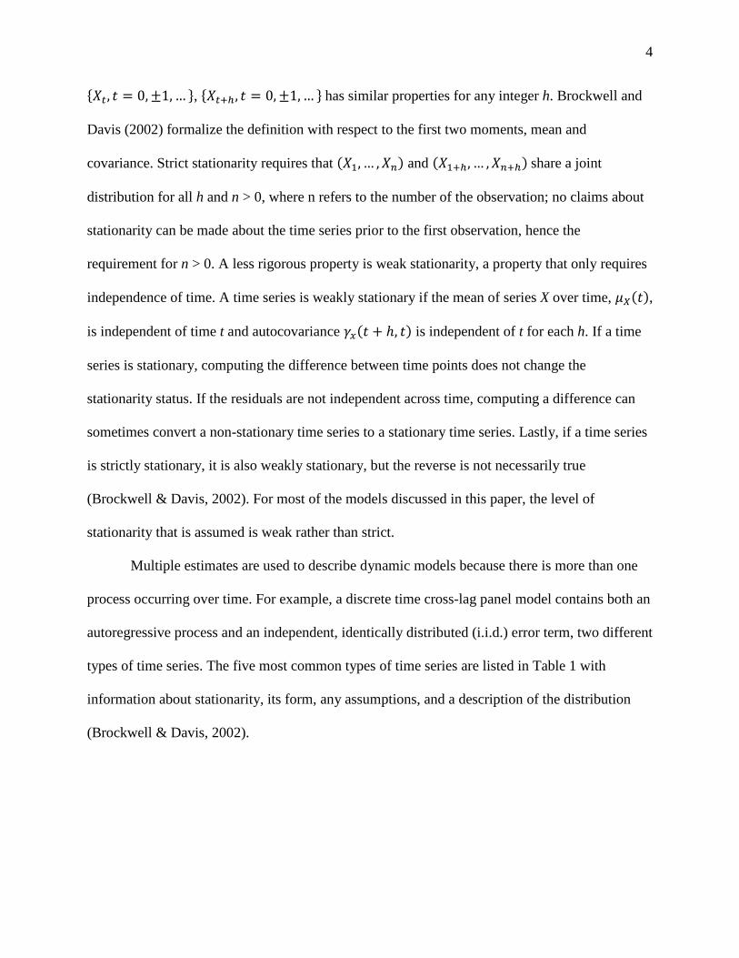
types of time series. The five most common types of time series are listed in Table 1 with

information about stationarity, its form, any assumptions, and a description of the distribution

(Brockwell & Davis, 2002).

5

Table 1. Common time series models and their properties

Type Stationary Form Assumptions Distribution

i.i.d. Yes X1, X2, …, t = 1, 2, … σ2 < ∞ {𝑋𝑋𝑡𝑡}~𝐼𝐼𝐼𝐼𝐼𝐼(0,𝜎𝜎2)

White noise Yes X1, X2, …, t = 1, 2, … {𝑋𝑋𝑡𝑡}~𝑊𝑊𝑊𝑊(0,𝜎𝜎2)

Random walk

No St = X1 + X2 + … + Xt, t = 1, 2, …

X0 = 0 {𝑋𝑋𝑡𝑡}~(0, 𝑡𝑡𝜎𝜎2)

{𝑋𝑋𝑡𝑡}~𝐼𝐼𝐼𝐼𝐼𝐼(0,𝜎𝜎2)

Moving average

Yes Xt = Zt + θZt-1, t = 0, ±1, …

{𝑍𝑍𝑡𝑡}~𝑊𝑊𝑊𝑊(0,𝜎𝜎2) {𝑋𝑋𝑡𝑡}~�0,𝜎𝜎2(1 + 𝜃𝜃2)�

θ is a real number

Auto-regressive

Yes Xt = φXt-1 + Zt, t = 0, ±1, …

{𝑍𝑍𝑡𝑡}~𝑊𝑊𝑊𝑊(0,𝜎𝜎2)

|φ| < 1 for AR(1)

Zt is uncorrelated with Xs

The simplest of time series model is referred to as i.i.d., meaning independent, identically

distributed. These random variables are independent and uncorrelated with respect to time and

have a mean of 0 and finite variance. The simplest example would be the outcome of flipping a

fair coin where the outcome of a coin flip has no influence on any other coin flip and the

expected mean of a series (.5) was subtracted from the series. One flip of the coin is not expected

to be related to any other flip of a coin in the sequence. A time series very similar to i.i.d. time

series is the white noise time series, differing from i.i.d because the white noise time series does

6

not require independence from one observation to the next. All i.i.d. series are white noise time

series, but not all white noise time series are i.i.d. Mathematically for the white noise time series

𝑋𝑋𝑡𝑡, if the autocorrelation (standardized autocovariance) for 𝑋𝑋𝑡𝑡2 is 0, then the white noise is also

i.i.d. If the autocorrelation is not equal to 0, then it is only white noise. Random walk is the first

series described here that is additive in that the series St is composed of t individual time series

that added together determine the total effect, as seen in Table 1. Each Xt in St is i.i.d. random

variables. Random walks are not stationary because although the mean is independent of time

with an expected value of 0 if the first time point is 0, the variance of the time series is dependent

on time (Brockwell & Davis, 2002).

The last two models listed in Table 1 are the moving average (MA) and the auto-

regressive (AR). MA models focus on the error term with the current value being related to the

error term from the previous time point. AR models depend on previous values of the variable

itself. The example of each model listed in the table are for MA(1) and AR(1) respectively

though other numbers could be listed in the parentheses to indicate the number of coefficients

that will be estimated and how long across time observations relate to each other. In this case, the

use of the number 1 indicates that only the previous time point is predicting the current time

point. As seen in Table 1, MA(1) is defined by white noise at the current time point and some

coefficient θ that is multiplied by a white noise term from the previous time point. These terms

are additive. Similarly, for AR(1), the process Xt is defined by a white noise term added to a

coefficient φ multiplied by Xt-1. If |φ| < 1, then the process is stationary. Also, previous values of

X are independent from the white noise in the model (Brockwell & Davis, 2002).

With AR and MA models, we see that white noise processes are additive pieces in each

model. Likewise, AR and MA models can be combined to build an auto-regressive moving

7

average (ARMA) model that are denoted by ARMA(p, q) where p refers to the auto-regressive

process and q refers to the moving average process. ARMA(1, 1) is represented by

𝑋𝑋𝑡𝑡 = 𝜑𝜑𝑋𝑋𝑡𝑡−1 + 𝑍𝑍𝑡𝑡 + 𝜃𝜃𝑍𝑍𝑡𝑡−1 (2)

where φ is the auto-regressive coefficient between Xt and Xt-1 and θ is the moving average (white

noise) coefficient for the previous time point. Zt, white noise, is modeled as a constant

(Brockwell & Davis, 2002).

Estimation. Time series models where the errors are normally distributed are obtained

from univariate stochastic model preliminary estimation (USPE) (Box & Jenkins, 1976),

estimation that returns moments. USPE is a conditional likelihood, conditional both on white

noise from the current time point and on values that were not observed but are assumed to have

occurred before data was collected. USPE can be estimated with least squares, moment estimates

from or maximum likelihood (ML). In small samples, least squares estimates are negatively

biased but bias decreases as sample size increases. Least squares estimates are consistent and

estimates are normally distributed and close to maximum likelihood values, unless the series

contains a seasonal component; unconditional sum of square should be computed in models with

seasonal data because it will be more accurate, particularly in the case of short time series where

the conditional estimation drops one time point from the estimation process but the unconditional

estimation does not.

Although most time series in economics and political science articles reviewed for this

paper focus on time series models with manifest (observed) variables, it is possible to estimate a

structural equation modeling (SEM) ARMA time series by specifying a covariance matrix as

demonstrated by van Buuren (1997), work that was evaluated and extended in two studies by

Hamaker, Dolan, and Molenaar (2002; 2003). van Buuren’s simulation showed problems with

8

MA models that Hamaker and colleagues attributed to non-invertible series or series with values

near the boundary of invertible values (2002). A non-invertible series is one in which

observations not close to the current time point have a strong influence on the current time point;

the MA coefficient |θ| > 1. An invertible series has a |θ| < 1 indicating that as time passes, distant

observations cease to influence current observations. Hamaker et al. (2002) also showed that

model estimates were not maximum likelihood estimates as van Buuren claimed but USPE

estimates, although the results would be identical for ARMA(p, 0) models.

Sample size. Sample size in the context of a single time series refers to the number of

time points. Brockwell and Davis (2002) recommended as few as 30 time points though the

number of time points is dependent on the properties of the series being modeled. Erratic

estimates may be produced by time series with only 20 or 30 observations (Beck & Katz, 1996).

Hamaker, Dolan, and Molenaar (2003) simulated series of length t = 100 for n = 1 and t = 35 for

n = 5. They recommended that for n = 1 more than 50 time points are needed.

Extensions. Two extensions of the time series models that are relevant in this paper are

multivariate time series and cross-sectional time series. Multivariate time series measure the

person (or any single unit) on more than one variable over time, and relationships can be

specified between the variables over time. If the series are weakly stationary, the series are

referred to as Xt = (Xt1, Xt2)′ with a vector of means

𝝁𝝁 = 𝐸𝐸[𝑋𝑋𝑡𝑡] = �𝐸𝐸𝑋𝑋𝑡𝑡1𝐸𝐸𝑋𝑋𝑡𝑡2� (3)

with a covariance matrix

𝛤𝛤(ℎ) = 𝐶𝐶𝐶𝐶𝐶𝐶(𝑿𝑿𝑡𝑡+ℎ,𝑋𝑋𝑡𝑡) = �𝛾𝛾11(ℎ) 𝛾𝛾12(ℎ)

𝛾𝛾21(ℎ) 𝛾𝛾22(ℎ)� (4)

where the estimation of the correlation between two different time points (i ≠ j) is

9

𝜌𝜌�𝑖𝑖𝑖𝑖(ℎ) = 𝛾𝛾�𝑖𝑖𝑖𝑖(ℎ) �𝛾𝛾�𝑖𝑖𝑖𝑖(0)𝛾𝛾�𝑖𝑖𝑖𝑖(0)�−1 2⁄

. (5)

If estimating the correlation for the same time point (i = j), Equation 1 for the series

autocovariance is used (Brockwell & Davis, 2002). The second extension of a basic time series is

the cross-sectional time series where time series data has been collected on a sample or

population (Stimson, 1985). The number of observations are usually large enough to analyze

each series in isolation, but analyzed together, questions about inter-individual variation can be

addressed (Kennedy, 2008). If the sample exceeds the number of time points and more than one

outcome variable is included in the model, this is typically referred to as a panel model or cross-

lag panel model (CLPM). In a model with two outcome variables, they regress on each other

over time, either unidirectional or bidirectional (Kline, 2011). CLPMs can be extended to include

other predictors and to test mediating relationships.

Cross-lag panel model. Stimson (1985) referred cross-sectional time series as pooled

space and time analyses, and he called the model generalized least squares (GLS) ARMA.

Specifically, the error term consists of block Toeplitz matrices like van Buuren (1997) and

Hamaker et al. (2002) used to create a covariance structure for SEM estimation of time series.

The basic form of the GLS ARMA contains a predictor xit and an error term, εit:

𝑦𝑦𝑖𝑖𝑡𝑡 = 𝑥𝑥𝑖𝑖𝑡𝑡𝛽𝛽 + 𝜀𝜀𝑖𝑖𝑡𝑡 (6)

where i stands for the number of observations ranging from 1 to n; t is the number of time points.

In Equation 6, the 𝑦𝑦𝑡𝑡−1is a not a predictor for 𝑦𝑦𝑡𝑡. Instead, the autoregressive component is

modeled in the error term. For εit, the matrix version is referred to as Ε. The error matrix is

𝜠𝜠 =

⎣⎢⎢⎡𝜎𝜎1

2𝐴𝐴 0 ⋯ 00 𝜎𝜎22𝐴𝐴 ⋯ 0⋯ ⋯ ⋯ ⋯0 0 ⋯ 𝜎𝜎𝑛𝑛2𝐴𝐴⎦

⎥⎥⎤

(7)

10

where σ2 is estimated n times for heterogeneity across units, and auto-regressive matrix A is a

matrix with band diagonal elements specified with one unique parameter, ρ:

𝑨𝑨 =

⎣⎢⎢⎡ 1 𝜌𝜌 𝜌𝜌2 ⋯ 𝜌𝜌𝑡𝑡−1

𝜌𝜌 1 𝜌𝜌 ⋯ 𝜌𝜌𝑡𝑡−2⋯ ⋯ ⋯ ⋯ ⋯𝜌𝜌𝑡𝑡−1 𝜌𝜌𝑡𝑡−2 𝜌𝜌𝑡𝑡−3 ⋯ 1 ⎦

⎥⎥⎤.

(8)

Many variations of the Toeplitz block error structure have developed and tested, one of

which that uses OLS with a panel corrected error structure (Beck & Katz, 1996). Beck and Katz

also proposed a model that included both a lagged dependent variable (LDV) and a term to

handle serially correlated errors. The errors were correlated due to inclusion of a dynamic

process as a predictor in the model and they wanted to specify a model whose predictors were

independent of the error term. Because the error is now independent, GLS estimation is not

needed in order to obtain unbiased estimates. The LDV is

𝑦𝑦𝑖𝑖𝑡𝑡 = 𝜌𝜌𝑦𝑦𝑖𝑖(𝑡𝑡−1) + 𝛽𝛽1𝑥𝑥𝑖𝑖𝑡𝑡 − 𝛽𝛽2𝑥𝑥𝑖𝑖(𝑡𝑡−1) + 𝜀𝜀𝑖𝑖𝑡𝑡. (9)

This equation models AR(1) explicitly with 𝜌𝜌𝑦𝑦𝑖𝑖(𝑡𝑡−1) term as a predictor for 𝑦𝑦𝑖𝑖𝑡𝑡; β1 is the

coefficient for 𝑥𝑥𝑖𝑖𝑡𝑡, a variable that measures an AR(1) process as well so its t-1 term was also

included as a predictor; and any MA process captured by εit contains i.i.d. errors. Instead of Z for

the white noise error process, the error term is represented by εit because its notation is more

familiar outside of time series models and because the error term is assumed to be i.i.d. but not

necessarily white noise. Beck and Katz called it the static model. Keele and Kelly (2006)

modified this formula so that x is clearly another time series that is serving as a predictor:

𝑦𝑦𝑖𝑖𝑡𝑡 = 𝜌𝜌𝑦𝑦𝑖𝑖(𝑡𝑡−1) + 𝛽𝛽𝑥𝑥𝑡𝑡 + 𝑢𝑢𝑡𝑡, (10)

𝑥𝑥𝑡𝑡 = 𝛼𝛼𝑥𝑥𝑡𝑡−1 + 𝜀𝜀1𝑡𝑡, and

𝑢𝑢𝑡𝑡 = 𝜑𝜑𝑢𝑢𝑡𝑡−1 + 𝜀𝜀2𝑡𝑡.

11

The outcome is predicted by its previous time point and the auto-regressive coefficient, a single

𝑋𝑋𝑡𝑡 term with coefficient β and error term ut. Moving to the second formula, α is the

autoregressive term for xt and it has 𝜀𝜀1𝑡𝑡~𝐼𝐼𝐼𝐼𝐼𝐼(0,𝜎𝜎2). In comparison to Equation 9, the concurrent

predictor 𝑥𝑥𝑖𝑖𝑡𝑡 is missing; only the previous time point with its auto-regressive coefficient is

modeled. The error term ut consists of an autoregressive parameter in the error process plus

𝜀𝜀2𝑡𝑡~𝐼𝐼𝐼𝐼𝐼𝐼(0,𝜎𝜎2). Note that Equation 10 has three autoregressive parameters and is preferred over

the LDV is the error term is not i.i.d. (Keele & Kelly, 2006).

Estimation. For the model that Stimson (1985) described, GLS is used to obtain

estimates. The model is generalized because weighting is used to model heteroscedasticity across

the cross sections in the σ2 terms of the matrix Ε. Hamaker and colleagues (2003) used

maximum likelihood estimation with the raw data to produce estimates for n ≥ 1 and t > n. The

process they demonstrated took advantage of full information maximum likelihood estimation

(FIML), a process that easily handles missing or differing numbers of observations.

Extensions. If the research question being asked with panel data concerns dynamics, then

Kennedy (2008) recommends that a lagged version of the outcome should be included as a

predictor, like Equations 9 and 10, and be long enough to show the pattern repeat. Other

additions include time invariant and time-varying predictors. Time-invariant predictors, such as

gender, race, or treatment group, are measured once and apply equally to all time points. Time-

varying predictors, such as size of classroom, differ across time but are not expected to have their

own autoregressive effects. These predictors differ from the predictor xit in Equation 10 because

xit regresses on the previous time point.

Panel models were initially specified as single level models but recent research has

shown that those models are likely to be misspecified. Instead, we should be considering random

12

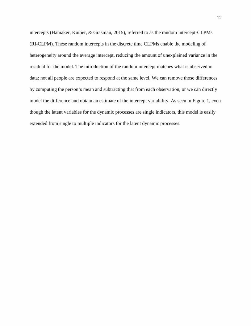
intercepts (Hamaker, Kuiper, & Grasman, 2015), referred to as the random intercept-CLPMs

(RI-CLPM). These random intercepts in the discrete time CLPMs enable the modeling of

heterogeneity around the average intercept, reducing the amount of unexplained variance in the

residual for the model. The introduction of the random intercept matches what is observed in

data: not all people are expected to respond at the same level. We can remove those differences

by computing the person’s mean and subtracting that from each observation, or we can directly

model the difference and obtain an estimate of the intercept variability. As seen in Figure 1, even

though the latent variables for the dynamic processes are single indicators, this model is easily

extended from single to multiple indicators for the latent dynamic processes.

13

Figure 1. Random intercept-cross-lag panel model. The paths of ξx and ξy on each time point of the respective dynamic process is fixed to 1 to enable the estimation of the random intercept. The paths from the latent dynamic variables X and Y to the observed indicators xt and yt are fixed to 1 for identification purposes with all other parameters freely estimated. Depending on the number of time points, the correlations between the disturbances may need to be equated to estimate a model with sufficient degrees of freedom.

Discrete versus continuous time

Discrete time series and CLPMs are popular, but they do have one assumption

that is challenging to meet: all time points are equally spaced. In psychological research, it is

challenging to collect data more than once from an individual much less repeatedly at regular

x1 x

2 x

3 x

4 x

5

y1 y2 y3 y4 y5

σY

1

1

ξy

ξx

1

1 1

1 1

1

1

1

Y1 Y2 Y3 Y4 Y5

1

1

X1 X2 X3 X4 X5

σX

σY

σX3

σY

σX

σY

σX

1 1 1 1 1

1 1 1 1 1

σX1

σY1

σ

σ

14

intervals. Sometimes this condition is met but what is meant by one unit of time can differ across

research studies. One researcher could take weekly observations and a second researcher could

take semi-monthly or monthly observations. With two different time frequencies, it can be

challenging to compare results between two studies. By shifting to continuous time, results from

those two studies can be compared because estimates describe the underlying process rather than

results tied to a specific unit of time. Discrete time estimates for any unit of time are related to

continuous time estimates through e, the base of the natural logarithm:

𝐀𝐀(∆𝑡𝑡𝑖𝑖) = 𝑒𝑒𝑨𝑨#∙∆𝑡𝑡𝑖𝑖. (11)

A refers to the autoregressive and cross-lag matrix for some lag of time Δt for individual i; the

autoregressive values are listed on the diagonal and cross-lag values are listed on the off-

diagonal. A# is the drift matrix, the continuous time A matrix of auto-effects and cross-effects,

where the autoregressive terms become auto-effects and cross-lags become cross-effects. A and

A# are both square matrices. Eigenvalues are computed when taking the logarithm of a matrix,

and the process to identify the eigenvalue uses all elements of a matrix.

An A matrix that is 1 x 1 contains the autoregressive term for a single dynamic process.

Computing the natural logarithm of A to obtain A# will always result in the same eigenvalue and

corresponding auto-effect in A# because there are no other elements in the matrix to influence the

calculation of the eigenvalue. For example, if A = 0.8, then A# = -0.22. With the introduction of

another dynamic process, A and A# become 2 x 2 matrices. All four elements are used in the

computation of the eigenvalues that are used to obtain the logarithm of a matrix so if any one of

the four elements changes in A, then every element in A# could be different. For example, as

shown in Table 2, an autoregressive value of 0.80 equals auto-effects that range from -0.14 to -

0.33, depending on the values of the other three elements in the matrix.

15

Table 2. Example of discrete time A matrix relationship to continuous time drift matrix A#

A A#

�𝑋𝑋1 𝐶𝐶𝑜𝑜 𝑋𝑋2 𝑋𝑋1 𝐶𝐶𝑜𝑜 𝑌𝑌2𝑌𝑌1 𝐶𝐶𝑜𝑜 𝑋𝑋2 𝑌𝑌1 𝐶𝐶𝑜𝑜 𝑌𝑌2

� �𝑋𝑋1 𝐶𝐶𝑜𝑜 𝑋𝑋2 𝑋𝑋1 𝐶𝐶𝑜𝑜 𝑌𝑌2𝑌𝑌1 𝐶𝐶𝑜𝑜 𝑋𝑋2 𝑌𝑌1 𝐶𝐶𝑜𝑜 𝑌𝑌2

�

�0.80 0.400.30 0.77� �−0.33 0.55

0.41 −0.37�

� 0.80 0.40−0.30 0.77� �−0.14 0.48

−0.36 −0.17�

� 0.80 −0.40−0.30 0.77� �−0.33 −0.55

−0.41 −0.37�

�0.80 0.000.10 0.77� �−0.22 0.00

0.13 −0.26�

Exact discrete model

The exact discrete model (EDM) takes a very direct approach to the estimation of

the continuous time cross-lag panel model with the estimation of a differential equation that is

related to a discrete time cross-lag panel model. Oud and Jansen (2000) introduced the EDM

estimated as a structural equation model, referring to the model as a continuous time state space

model. Described more broadly as a multivariate stochastic differential equation by Driver, Oud,

and Voelkle (n.d.), the model is the same as the one described by Voekle and colleagues in

previous papers (Voelkle & Oud, 2013; Voelkle, Oud, Davidov, & Schmidt, 2012). The model

still results in discrete time parameters being constrained to the corresponding continuous time

values, and discrete time estimates will be equivalent to the EDM estimates provided time

intervals are equal (Voelkle & Oud, 2015). The model is flexible enough to model observed

variables through single indicator constructs or multiple indicator latent variables however single

indicator constructs limit the ability to separate measurement error. The description of the EDM

16

that follows first reviews the discrete time cross-lag panel model with exogenous predictors

before describing the EDM.

In matrix form, the discrete time cross-lag panel model of order one (AR1) with

exogenous predictors is

𝜂𝜂𝑖𝑖 = 𝐀𝐀𝜂𝜂𝑡𝑡−1 + 𝐁𝐁𝑧𝑧𝑖𝑖 + 𝐌𝐌𝜒𝜒𝑡𝑡−𝑖𝑖 + 𝐖𝐖𝑖𝑖 . (12)

The measurement of a variable 𝜂𝜂𝑖𝑖 at any time is equivalent to that weighted variable at the

previous time point plus time invariant predictor z, time-varying predictor χ, and an error term W.

The coefficient matrix A provides the degree to which each outcome is related to previous

observations of η and other outcome variables; the matrix contains autoregressive coefficients on

the diagonal and cross-lag coefficients on the off-diagonal. The error term is represented by W,

a change in notation from ε to reflect the stochastic error term modeled using the Weiner process

in continuous time (Driver et al., n.d.).

In continuous time, the EDM stochastic differential equation is very similar to the

formula above. The derivative with respect to time, (dt) is

𝑑𝑑𝜂𝜂𝑖𝑖𝑡𝑡 = (𝑨𝑨𝜂𝜂𝑖𝑖𝑡𝑡 + 𝜉𝜉𝑖𝑖 + 𝑩𝑩𝑧𝑧𝑖𝑖 + 𝑀𝑀𝝌𝝌𝑖𝑖𝑡𝑡)𝑑𝑑𝑡𝑡 + 𝑮𝑮𝑑𝑑𝑾𝑾𝑖𝑖𝑡𝑡 . (13)

The vector of outcomes is η for subject i at time t. The A matrix contains auto-effects and cross-

effects, estimates of the relationship of the outcome variables over time. The term representing

the random intercept is ξ with mean of κ and variance φξ. The mean κ is the long-term intercept

of the process, like to the fixed intercept, and the variance φξ is the estimate of how individuals

differ from the average, similar to a random effect. B is the matrix of time invariant predictors,

and M is the matrix of effects of time-varying predictors on ηit. These time-varying predictors are

assumed to have no auto-effects from one time point to the next time point; otherwise they

should be modeled as another endogenous process instead of as a time-varying predictor. As

17

described by Driver and colleagues (n.d.), time-varying predictors that estimate short term

effects is an impulse. The Dirac delta, a function that is infinity at 0 and 0 elsewhere with an area

of 1, is used to estimate the effect of this impulse as follows:

𝜒𝜒𝑖𝑖𝑡𝑡 = � 𝑥𝑥𝑖𝑖𝑖𝑖𝛿𝛿𝑡𝑡−𝑖𝑖𝑖𝑖∈𝑈𝑈𝑖𝑖

. (14)

The interval of time is represented from t-1 to t though time intervals can vary across individuals.

Computationally, for a specific interval of time that maps the discrete time observations to the

continuous time estimates, the solution to the stochastic differential equation is

𝛈𝛈𝑖𝑖𝑡𝑡 = 𝑒𝑒𝐀𝐀∙𝛥𝛥𝑡𝑡𝛈𝛈𝑖𝑖𝑡𝑡0 + 𝐀𝐀−1[𝑒𝑒𝐀𝐀∙𝛥𝛥𝑡𝑡 − 𝐼𝐼]𝛏𝛏𝑖𝑖 + 𝐀𝐀−1[𝑒𝑒𝐀𝐀∙𝛥𝛥𝑡𝑡 − 𝐼𝐼]𝐁𝐁𝐳𝐳𝑖𝑖

+ � 𝑒𝑒𝐀𝐀∙(𝑡𝑡−𝑠𝑠)𝐌𝐌𝛘𝛘𝑖𝑖(𝑠𝑠)𝑑𝑑𝑠𝑠 + � 𝑒𝑒𝐀𝐀(𝑡𝑡−𝑠𝑠)𝐆𝐆𝑑𝑑𝐖𝐖𝑖𝑖(𝑠𝑠)𝑡𝑡

𝑡𝑡0

𝑡𝑡

𝑡𝑡0.

(15)

Each term in this equation has a one-to-one mapping to Equation 12. The dynamic processes in η

for individual i over time t are the sum of the drift matrix plus the random intercept ξi, the time-

invariant predictors zi, the time-varying predictors 𝛘𝛘𝑖𝑖, and the stochastic error term G. For

estimation, the time-varying term is replaced as with a summed term based on the Dirac delta

defined in Equation 14 (Driver et al., n.d.).

The error process for EDM is a stochastic error process that is a continuous time random

walk, referred to as the Weiner process, hence the use of W for the error term in Equations 12

and 13. Recall from Table 1 that a random walk is a non-stationary process because its variance

is proportional to time so the error term in the EDM is non-stationary. The integral with respect

to s represents the stochastic process for the continuous time process. G is the Cholesky

decomposition, a lower triangular matrix that is positive definite satisfying the equation Q =

18

GG*. G* is the conjugate transpose and Q will contain the covariance matrix of error terms

(Driver et al., n.d.).

𝑐𝑐𝐶𝐶𝐶𝐶 �� 𝑒𝑒𝐀𝐀(𝑡𝑡−𝑠𝑠)𝐆𝐆𝑑𝑑𝐖𝐖(𝑠𝑠)𝑡𝑡

𝑡𝑡0� = � 𝑒𝑒𝐀𝐀(𝑡𝑡−𝑠𝑠)𝐐𝐐𝑒𝑒𝐀𝐀𝑇𝑇(𝑡𝑡−𝑠𝑠)𝑑𝑑𝑠𝑠

𝑡𝑡

𝑡𝑡0

(16)

Equation 17 is the result of integrating Equation 16 where a Kronecker product ⊗ , with

A# = A ⊗ I + I ⊗ A, is used transform Equation 16 into a matrix format for computation. The

equation is

� 𝑒𝑒𝐴𝐴(𝑡𝑡−𝑠𝑠)𝑄𝑄𝑒𝑒𝐴𝐴∗(𝑡𝑡−𝑠𝑠)𝑑𝑑𝑠𝑠𝑡𝑡

𝑡𝑡0= 𝑖𝑖𝑟𝑟𝐶𝐶𝑖𝑖 �𝐴𝐴#

−1[𝑒𝑒𝐴𝐴#∙∆𝑡𝑡 − 𝐼𝐼]𝑟𝑟𝐶𝐶𝑖𝑖(𝑄𝑄)� (17)

where irow is the inverse of the row operation and the row operation takes row entries and places

them in a column vector (Driver et al., n.d.).

Predictors. Time-invariant and time-varying predictors can be included in the EDM.

Time-invariant predictors are not expected to change over time, or at least over the range of time

that is modeled for the dynamic processes. With the inclusion of time-invariant predictors,

estimates can be obtained for the effect of that predictor in continuous time, the asymptotic effect

of the total increase in the process that is expected from a one-unit increase in the predictor, and

the amount of variance and covariance in the outcomes that is associated with all time-invariant

predictors. In the EDM, the variance associated with time-invariant predictors are expected to

directly predict the dynamic process.

19

Figure 2. Exact discrete model with time-invariant predictor and trait variance. The trait variance predicts the latent dynamic process. For multiple indicator models it is possible to estimate trait variance for the manifest variables instead of the latent variables.

Time-varying predictors can be modeled in one of two ways, as a short-term effect or as a

long-term effect (Driver et al., n.d.). A short-term effect is an impulse that is not expected to

change the long-term level of a process. A long-term effect is expected to change the overall

level of the process by raising or lowering it. How this predictor should be modeled depends on

the research question. If the researcher is interested in both short term and long term effects, then

two separate models would need to be estimated because it is not possible to simultaneously

x3 x

2 x

4 x

5

y1 y5

1

1

ξy

ξx

Y1 Y2 Y3 Y4 Y5

X1 X2 X5

Time-Invariant Predictor

σX3

σY

σX

σY

σX

1 1 1 1 1

1 1 1 1 1

σY

x1

y3 y4 y2

σY σY

X3 X4

σX

20

obtain estimates about short- and long-term effects from the EDM. In a model for short-term

effects, estimates of the time-varying predictor’s effect on the process, and its covariance with

the initial time point, trait variance, and time-invariant predictors can be obtained. To estimate

long-term effects, this time-varying effect becomes another process in the drift matrix though

only latent with an auto-effect near zero, and no covariance estimates with the initial time point,

trait variance, or other predictors.

Unlike time-invariant predictors, time-varying predictors are expected to have different

values at each time point. The EDM returns a single parameter estimate reflecting its continuous

time effect on the dynamic process. The other assumption about time-varying predictors is that

they do not have a detectable auto-effect. In other words, each observation should be unrelated to

the next at the time of measurement. An example of an appropriate time-varying predictor is a

repeated measures study design where the participant randomly receives the treatment or control

condition at each time point. If the time-varying variable does have a measurable auto-effect,

then it should be modeled as part of the drift matrix to correctly specify its dynamic process

(Driver et al., n.d.).

Trait variance. Trait variance is estimated in EDM to account for heterogeneity in the

intercept, like the random intercept term in RI-CLPM. When single indicators are used to model

the dynamic process, heterogeneity is estimated for the latent dynamic process, as reflected in

Figure 2. In a model with multiple indicators, Driver et al. (n.d.) recommend estimating

heterogeneity for the manifest variables as that may improve model fit and more accurately

reflect where in the model heterogeneity would be observed in the data.

Model limitations. The EDM assumes stationarity though there are options for modeling

non-stationarity in the mean. Change in variance over time can only be modeled via an

21

exogenous time-varying predictor as described above. The model assumes that the data follows a

multivariate normal distribution, as expected given models are fit with full information

maximum likelihood. Only heterogeneity in the intercept can be modeled though heterogeneity

in slopes due to known group membership can be estimated with multiple group models (Driver,

Oud, & Voelkle, n.d.). In simulations conducted by Oud and Singer (2008), EDM was shown to

produce unbiased, efficient estimates as compared to a Kalman filter estimation of the equivalent

system in a two variable cross-lag model but to date nothing has been published regarding the

extended model.

Omitted variables

Specification errors may occur because a key explanatory variable was not included in a

model or time was specified as a linear term when a higher order polynomial would more

accurately represent the how the outcome changes longitudinally. But little is known about

omitted variables in a continuous time context. The review that follows focuses on what we do

know about omitted variables in regression-based methods to gain insight as to how omitted

variables might impact continuous time estimates and standard errors.

Single level regression. Omitted variables, also known as left out variable error (Mauro,

1990), may result in biased parameter estimates and incorrect standard errors in OLS and other

regression-based methods. How other estimates are impacted depend on whether the omitted

variable is orthogonal to other predictors in the model or not. These omissions can in turn lead to

either Type I or Type II errors. In the case of an omitted variable that is orthogonal to the other

predictors but related to the outcome, the coefficients for the other predictors will be unbiased

but have standard errors that are too large when compared to a model with all relevant variables

included in the model (Cohen, Cohen, West, & Aiken, 2003). The variance associated with the

22

omitted variable will be unexplained variance and part of the error term. Omitted predictors that

are related to the outcome and another predictor in the model will result in an error term that is

not independent of that predictor (Kennedy, 2008). The included predictor’s coefficient will be

biased provided the effect is sufficiently large on the predictor and the outcome (Mauro, 1990).

James (1980) highlighted the problem with omitted variables in path analysis when the

assumption of independence between the error term and endogenous outcomes in the model is

violated, a violation that occurs due to omitted variables. In a simple model with a standardized

single predictor (x) and outcome (y) that should include an omitted mediator (u for unmodeled),

the standardized coefficient of the outcome will be biased by the product of the correlation

between the predictor and the omitted variable and the standardized coefficient for the path from

the omitted variable to the final outcome, rxuβu. If the x and u are uncorrelated or the omitted

variable is not related to the outcome y, this bias reduces to 0. The only caveat James mentioned

to this equation was in the case of a suppressor variable. Suppression occurs when a new

predictor is added to the model that is related to other predictors in the model but not the

outcome. Omission of the new predictor will result in an estimate of x on y that is too small

(Cohen et al., 2003). Aside from considering how the omitted variable will impact estimates,

James draws attention to the strength of the effect that the omitted variable has on the outcome

and the degree to which x and u are correlated. If either coefficient or correlation are weak or

near 0, the bias in the model with be small or none. The other case where omission will not

negatively impact the model is when x and u are highly correlated. In that case, the standard

errors would be inflated for two highly correlated predictors (|r| > 0.90) in the model. The best

modeling choice in that circumstance would be the omission of one of the predictors.

23

Mauro (1990) who investigated left out variable error declined to quantify the bias,

saying instead that there are too many factors to know exactly how an omitted variable would

impact the estimates in the model. Similar to James (1980), Mauro discussed how the omitted

predictor is related to other variables in the model determines whether the omitted variable will

impact results or not. The three criteria are a substantial effect on the outcome, a substantial

correlation with another predictor, and orthogonal to all other predictors. The piece discussed by

Mauro was how the omitted variable is related to all of the predictors, not just a single predictor.

If the omitted variable is correlated with several predictors in the model, then its variance will be

represented in each predictor and so the impact of its omission should be minimized. So, it is

only when the omitted variable represents variance that none of the other predictors are

measuring that results will be biased.

Multilevel models. With the transition to multilevel models, the number of parameters

that can be impacted by omitted variables is greatly increased. With respect to mediation

modeling, the indirect effect, the level-2 variance-covariance matrix, and the total effect are

impacted if the omitted variable is a level 2 variable (Tofighi, West, & MacKinnon, 2013). In

addition to the fixed estimates in a multilevel model, random effects can be included in the

model specification. Beck and Katz (1996) view statistically significant random effects in cross-

sectional time series, time series based on a cross-section of people with more time points than

people, as a sign of an omitted variable. In other words, an omitted variable is causing the

additional variance around the estimate; if that omitted variable can be identified, then the

random effect would no longer be needed. Raudenbush and Bryk (2002) discuss how omitted

variables can result in bias but also where the model is robust to omissions. If a level 1 predictor

is omitted, and it relates to both the outcome and another predictor in the model, then one or

24

more coefficients in the model will be biased. If the predictor is continuous, then all coefficients

will be incorrect. When all of these conditions hold but the other predictor in the model is also

part of a cross-level interaction, these results will be confounded. Kennedy (2008) stated that if

fixed and random effects are statistically equal in their effect, then omitted variables will not

impact random effect estimates.

The most recent work in panel models was conducted by Hamaker and colleagues (2015)

in which they showed the necessity of a random intercept term in a CLPM. This term is needed

to separate within from between effects of the dynamic process. The heterogeneity in the

intercept is due to unmeasured variables affecting the level of the process. Without this term, the

cross-lags can have coefficients that are the negative when they should be positive, or vice-versa.

The process that appears to drive another dynamic process may be actually be driven instead.

Lastly, without the random intercept, conclusions about the dynamics could result in Type I or

Type II errors.

Measurement error and the exact discrete model

All of the research discussed in this paper applies to cross-sectional models and discrete

time-series models. Variance from omitted variables typically become unexplained variance in

the model (Cohen et al., 2003), and aside from interactions, non-differentiable from

measurement error. Previous research shows that this increased measurement error, if not

modeled, can result in biased drift parameter estimates in the EDM if the cross-lags are both

positive (Shaw, 2015); the cross-effects will also be overestimated, becoming more biased as

measurement error increases. If either cross-effect is negative, the estimates are not impacted by

the measurement error. Auto-effects will be underestimated regardless of whether the cross-

effects are positive or negative. Turning to systems literature where the first derivative is

25

interpreted as representing positive feedback or negative feedback can provide insight into these

findings. The first derivative is the rate of change, also known as the slope in regression models.

When the first derivative is positive, then the function is increasing; when the first derivative is

negative, the function is decreasing (Granville, Smith, & Langley, 1957). In a panel model, if

both variables have positive cross-effects and those effects are additive across time, the processes

being measured can become increasingly unstable. If either variable is decreasing instead of

increasing, the processes stabilize. So, in the case of measurement error, robust estimates can be

obtained from a stable process but not from an unstable process. However, outside influences

should also be considered when evaluating what in isolation what would appear to be an unstable

process. Adding an input from the outside to an unstable system can add stability (Åström &

Murray, 2008), such as the rudder added to the first airplane. In reality for non-mechanical

systems, such as those studied by psychologists, there are always outside influences. Whether

those outside influences are included in the model or not often depends on the research question.

When the impact of measurement error study on EDM was evaluated (Shaw, 2015), trait

variance was not estimated in the model so it is unclear whether the all parameter estimates

would have been robust to measurement error rather than just drift matrices with one or more

negative cross-effects. If the trait variance parameter in the EDM is modeling heterogeneity like

a random intercept, the effects of an uncorrelated omitted variable should be reflected in that

estimate. But, the differential equation solution for the EDM shown in Equation 11,

𝐀𝐀(∆𝑡𝑡𝑖𝑖) = 𝑒𝑒𝑨𝑨#∙∆𝑡𝑡𝑖𝑖,

highlights how all parameters in the model are impacted by the drift matrix, so the degree to

which other parameters are impacted is unclear. There is also the question of whether

26

coefficients for another predictor in the model will be biased. If they are uncorrelated, the other

predictor should be estimated without bias; we would expect bias when the predictor is

correlated with the omitted variable. If the variance is absorbed by the trait variance, only model

fit should change with zero bias for the estimates. Another open question is how the relationship

between the predictors influence the drift parameter estimates. Are the drift parameter estimates

robust to omitted variables as long as one cross-effect is negative, regardless of how the omitted

predictor is related to the other predictor or the outcomes?

Omitted variables and the EDM

Turning to research on omitted variables in regression provides insight on the limits a

random intercept term may have. In single level regression, the effects of omitted variables on

model estimates can impact standard errors resulting in Type I or Type II errors (Cohen et al.,

2003). Omitted variables can also result in predictors that are related to the error term, one type

of model misspecification that can also result biased coefficients (Kennedy, 2008). The degree to

which these problems occur depend upon the strength of relationship between the omitted

variable and other variables in the model (Mauro, 1990). In addition to strength impacting

estimates, suppression can also change how an omitted variable impacts a model. Characteristics

of the specific data set can change how an omitted variable effects model estimates.

Similarly, EDM continuous time estimates are sometimes biased when the data contains

measurement error. Whether the parameter estimates will be biased depends on characteristics of

the data set, in particular whether the cross-effects are positive or negative. If variance from an

omitted variable is treated in the estimation process like measurement error, then we can predict

how the model estimates will be impacted (Shaw, 2015). What is unknown about the EDM

estimated with the ctsem package (Driver et al., n.d.) is how the trait variance parameter will

27

account for heterogeneity in the intercept. Returning to the stochastic differential equation for the

EDM in Equation 15, every set of estimated parameters is impacted by the drift matrix. With the

influence of the drift matrix and omitted variables that may be related to included predictors, can

the trait variance account for omitted variable variance or at least reduce the bias so conclusions

would not be different from a correctly specified model?

To explore how omitted variable relationships with another predictor and the outcome

variables impact the drift parameters in the EDM, two simulations have been designed to test the

effects of an omitted variable on the drift matrix, both when the exogenous omitted predictor is

orthogonal to another predictor in the model and when they are related. A model that includes

trait variance and a time-invariant predictor was used for all simulation conditions.

The first simulation added a second time-invariant predictor to the data generation model

and this variable was then omitted. The impact on the drift matrix was evaluated as well as the

estimate for other time-invariant predictor. Regardless of the drift matrix values, some of the

estimates drift estimates are expected to be robust. When the omitted variable is related to the

other time-invariant predictor, drift parameters may still be robust but the size of the coefficient

for the time-invariant predictor was expected be biased. The trait variance is expected to increase

in the omitted variable condition, regardless of how the two predictors are correlated. Because

the time-invariant predictor is not correlated with the trait variance, it is not expected to absorb

all of the omitted variable variance.

The second simulation extended the first simulation by testing a time-varying predictor

that was omitted. The focus was on a time-varying predictor that has a short-term effect on the

system rather than one that represents a long-term effect. The time-varying predictor in the EDM

relates to the system dynamics and to the trait-variance, so the model may be robust to the

28

omission of a time-varying predictor when that predictor is also orthogonal to the time-invariant

predictor. That condition was tested along with models where the time-invariant and time-

varying predictor are correlated. Whether the drift parameter estimates are robust when one

predictor is omitted may depend on whether they have positive or negative effects on the drift

matrix and whether the two predictors were positively or negatively correlated in the data

generation model. Because trait variance models heterogeneity that may be due to other omitted

variables, then a time-varying predictor could be correlated with the other omitted predictor

variance represented in the trait variance. Therefore, the trait variance parameter is may absorb

more variance from the omitted time-varying predictor if the time-varying predictor was

correlated with the trait variance in the data simulation model.

29

Chapter 2: Methods

Experimental design

Two simulations were conducted to explore how omitted variables impact results from

the EDM, first with a time-varying omitted variable and second with a time-invariant omitted

variable. In order to mimic substantive research in which data is collected at discrete time points,

data was simulated against the discrete time random intercept – CLPM (Hamaker et al., 2015)

and then analyzed via the EDM in order to obtain continuous time estimates. Currently we do not

have enough information about omitted variables in the EDM to justify differing the conditions

between the time-varying simulation and the time-invariant simulation. So, unless explicitly

stated otherwise, all simulation conditions applied to both simulations.

Fixed conditions

Fixed simulation conditions are listed in Table 3, and they include number of time points,

latent dynamic variables indicators, predictors, and sample size. Number of time points and

indicators were not expected to impact simulation results that examined bias of latent parameter

estimates. A single time-invariant predictor was included to represent an exogenous predictor

that would be included by applied researcher, such as age or socio-economic status. Sample size

of 200 was selected to replicate the number tested by Hamaker and colleagues (2015) when

comparing the discrete time CLP to the RI-CLP. A single sample size is also being tested

because results in Shaw (2015) did not change significantly with respect to sample size.

30

Table 3. Fixed simulation conditions

Condition Count Comments

Time points 5 Time points were be equally spaced

Indicators per time point 1 A single-indicator model, reflecting a scenario

with a composite score rather than a multiple

indicator measurement model

Time invariant predictor 1 The predictor was regressed on by the random

intercept which in turn predicted the dynamic

outcomes.

Sample size 200 The number of observations was selected to

replicate the sample size simulation condition

used by Hamaker et al. (2015) when evaluating

the RI-CLPM.

The remaining fixed conditions applied to parameters that were be included in the data

simulation with a single value rather than a set of values. In order to constrain the number of

conditions tested, the latent autoregressive and random intercept parameters for X were

estimated for single values rather than a set of values for each parameter. The X autoregressive

parameter were set to 0.5, and the random intercept for X was set to 0.17. The time-invariant

predictor had a positive effect on both X and Y (β = 0.30 on X; β = 0.35 on Y), the two dynamic

variables in the model. The first time point had a variance of 1 and the disturbances around the

other time points were 0.1, as shown in Figure 3, a diagram of the RI-CLPM that the model that

was used as the data generation model.

31

Figure 3. Data generation model. This model served as the set of fixed simulation conditions. An exogenous variable was then be omitted during the analysis. Drift matrix, additional exogenous predictors and random intercept variance varied. Varying conditions

Dynamics in the A-matrix, random intercepts, strength of omitted predictors, and

correlation between the omitted variable and the model time-invariant varied because little is

known about how the model misspecification would impact the estimates.

A-matrix values. The primary consideration on testable estimates for the auto-effects

and cross-effects is stationarity. Both X and Y need to be stationary processes but they also need

x1 x

2 x

3 x

4 x

5

y1 y2 y3 y4 y5

1

1

ξy

ξx

1

1 1

1 1

1

1

1

Y1 Y2 Y3 Y4 Y5

1

1

X1 X2 X3 X4 X5

.17

Time-Invariant

Predictor(s) .1

.1

.1

.1

.1

.1

1 1 1 1 1

1 1 1 1 1

0.30

0.35

1

1

.05 .05 .05 .05 .05 .1

.1

.01

.5 .5 .5 .5

32

to be vector stationary (Hamilton, 1994) meaning that the pair of processes are stationary, or

costationary. If the absolute values of both A-matrix eigenvalues are both less than 1 (|𝜆𝜆𝑖𝑖| < 1),

then the condition of costationarity is met. Because omitted variable variance is expected to

manifest as measurement error, results from Shaw (2015) were used to inform simulation

conditions. The A-matrix in discrete time with two constructs is composed of four values for a

lag of 1: X1 to X2 (auto-regressive), X1 to Y2 (cross-lag), Y2 to X1 (cross-lag), and Y1 to Y2

(auto-regressive). Because auto-effects estimates were shown to be stable regardless of true

cross-effect parameters, two auto-effects were tested for Y. The auto-regressive parameters were

tested with value of 0.50 for X and 0.30 and 0.60 for Y. Cross-lag parameters Yt+1 on Xt and Xt+1

on Yt took on the following pairs of values: (−0.30, -0.45), (−0.30, -0.25), (−0.30, 0.00), (−0.30,

0.25), (−0.30, 0.45), (0.30, 0.00), (0.30, 0.25), and (0.30, 0.45). So, all matrix combinations were

evaluated to ensure that only combinations with |𝜆𝜆𝑖𝑖| < 1 were included. With 2 varying

autoregressive parameters and 8 cross-lag combinations, 16 A-matrix conditions were evaluated.

As shown in Figure 4, these 16 matrices were further described as negative, positive, balanced,

and one-way to simplify the presentation of results in the next chapters. When referenced in the

results chapters, the 4 values of the matrix are listed in parentheses to clarify which of the 16

matrices is being discussed.

33

Figure 4. The four types of A-matrices grouped by cross-lag simulation conditions.

Random intercepts. Because intraclass correlations (ICCs) can vary widely, random

intercepts that correspond to 3 ICCs of size 0.20, 0.30, and 0.55 was tested. The formula for

calculating the ICC was rearranged to compute the random intercept term,

𝜏𝜏00 =𝜎𝜎 ∙ 𝐼𝐼𝐶𝐶𝐶𝐶

1 − 𝐼𝐼𝐶𝐶𝐶𝐶 (18)

where 𝜏𝜏𝑜𝑜𝑜𝑜 is the random intercept and 𝜎𝜎 is the variance of the outcome multiplied by the sum of

the disturbances. Taking into account the variance of the initial time point simulated to equal 1

and disturbances for each remaining time points estimated at 0.1, substituting ICCs into the

formula results in the following random intercepts: 0.10, 0.17, and 0.49. The random intercept on

X was fixed to 0.17. The random intercept on Y varied across the three levels.

Negative

Positive

One-way

Balanced

34

Omitted predictors

All of the fixed and varying conditions described above were tested in two simulations.

The first simulation evaluated models with an omitted time-invariant predictor. The second

simulation evaluated models with an omitted time-varying predictor. How these omitted

variables related to the time-invariant predictor differ in the data generation process, and this

difference was why the omission of each variable type is expected to impact the model in

different ways.

Omitted time-invariant predictor. Data was simulated with a time-invariant predictor

that was omitted in the estimation step of the simulation. The simulation model was almost

identical to that shown in Figure 1. Instead of a single, time-invariant predictor that was

exogenous to the model, there were two. Three correlations were tested between these two

predictors: r = 0, r = 0.3, and r = -0.3. The time invariant predictor was generated to have the

same effect on the two dynamic processes. The parameter conditions were near zero (−0.05),

negative (-0.3), and positive (0.3). Together the 3 correlation conditions paired with 3

coefficients resulted in 9 conditions listed in Table 4.

Table 4. Combinations of remaining simulation conditions

Simulation Condition

Time-invariant Correlation

Time-invariant Beta Coefficient

1 .00 −0.05 2 .00 −0.30 3 .00 0.30 4 −.30 −0.05 5 −.30 −0.30 6 −.30 0.30 7 .30 −0.05 8 .30 −0.30

35

Simulation Condition

Time-invariant Correlation

Time-invariant Beta Coefficient

9 .30 0.30

Data generation. With 16 different conditions for the A-matrix, 3 for the random

intercept, and 9 for the relationship of the omitted time-invariant predictor to other variables in

the model, this simulation consists of 432 between conditions. A mean value of 0 has been

selected for X, Y, and the predictors in the model. A uniform distribution was used to generate

seeds for data generation. For each condition, 1000 data sets were be generated in Mplus 7.3

(Muthén & Muthén, 1998-2015) and imported into R 3.3.1 (R Core Team, 2017). Once imported

to R, time intervals of 1 for equal spacing of time points were added, lag values required by the

EDM estimation function (Driver et al., n.d.).

Estimation. The ctsem package (Driver et al., n.d.) in R 3.2.0 (R Core Team, 2017) was

used to estimate three models with each data set. The first model generated continuous time

estimates for all variables that were included in the data simulation; this model is be referred to

as the full model. The second model, referred to as the one predictor model, omitted one time-

invariant predictor while retaining the time-invariant predictor with fixed simulation conditions.

The third model estimated just the dynamic process with the trait variance and was referred to as

the dynamic model. The drift matrix parameter estimates and confidence interval, trait variance,

predictor-related estimates, convergence status, and -2 Loglikelihood and degrees of freedom

will be saved from each model. Estimates for the predictors included the time-invariant effect on

the drift matrix, on the first time point for X and Y, and in the case of the two models the

variance-covariance matrix of the time independent predictors.

Analysis. After estimating the simulated data with the EDM, the logm function in the R

package expm (Goulet et al., 2015) was used to compute the log of the A(Δti) matrix for those

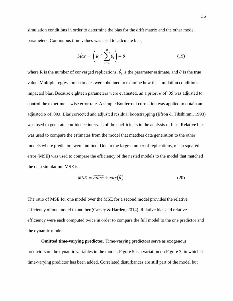
36

simulation conditions in order to determine the bias for the drift matrix and the other model

parameters. Continuous time values was used to calculate bias,

𝑏𝑏𝑏𝑏𝑏𝑏𝑠𝑠� = �𝑅𝑅−1�𝜃𝜃𝚤𝚤�𝑅𝑅

𝑖𝑖=1

� − 𝜃𝜃 (19)

where R is the number of converged replications, 𝜃𝜃𝚤𝚤� is the parameter estimate, and 𝜃𝜃 is the true

value. Multiple regression estimates were obtained to examine how the simulation conditions

impacted bias. Because eighteen parameters were evaluated, an a priori α of .05 was adjusted to

control the experiment-wise error rate. A simple Bonferroni correction was applied to obtain an

adjusted α of .003. Bias corrected and adjusted residual bootstrapping (Efron & Tibshirani, 1993)

was used to generate confidence intervals of the coefficients in the analysis of bias. Relative bias

was used to compare the estimates from the model that matches data generation to the other

models where predictors were omitted. Due to the large number of replications, mean squared

error (MSE) was used to compare the efficiency of the nested models to the model that matched

the data simulation. MSE is

𝑀𝑀𝑀𝑀𝐸𝐸 = 𝑏𝑏𝑏𝑏𝑏𝑏𝑠𝑠�2 + 𝐶𝐶𝑏𝑏𝑟𝑟�𝜃𝜃��. (20)

The ratio of MSE for one model over the MSE for a second model provides the relative

efficiency of one model to another (Carsey & Harden, 2014). Relative bias and relative

efficiency were each computed twice in order to compare the full model to the one predictor and

the dynamic model.

Omitted time-varying predictor. Time-varying predictors serve as exogenous

predictors on the dynamic variables in the model. Figure 5 is a variation on Figure 3, in which a

time-varying predictor has been added. Correlated disturbances are still part of the model but

37

were dropped from the figure in order to highlight how the time-varying predictor relates to the

other variables in the model. Parameter estimates for the predictor’s effect on the dynamic latent

variables were equated across time and the size of the effect on X should have been equal to the

size of the effect on Y in the simulation. The same three coefficients tested in the first simulation

were tested here. And like the first simulation, the time-varying predictor included a correlation

with the time-invariant predictor in the model. The 3 levels that were tested are r = 0, r = 0.3, and

r = -0.3. An additional simulation condition that was tested will be a correlation between the trait

variance and time-varying predictor. This condition was restricted to a correlation near 0 with

one trait variance parameter and 3 levels with the other trait variance parameter: r = 0, r = 0.3,

and r = -0.3.

Data generation. This simulation consists of 1296 conditions because of the addition of

the correlation between the time-varying predictor and the trait variance. Correlations between

time points for the time-varying predictor was fixed to 0 in the model, ensuring that any

estimated relationship would only be due to sampling variability in the data generating process.

The time-varying predictor was simulated to generate short-term effects, impulses, rather than

long-term effects, a change in level. Again, X, Y, and the predictors were simulated with a mean

of 0. Similarly, 1000 data sets were generated for each simulation condition in Mplus 7.3

(Muthén & Muthén, 1998-2015) with seeds drawn from a uniform distribution. After data

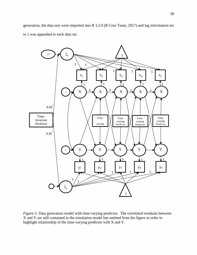
38

generation, the data sets were imported into R 3.2.0 (R Core Team, 2017) and lag information set

to 1 was appended to each data set.

Figure 5. Data generation model with time-varying predictor. The correlated residuals between X and Y are still contained in the simulation model but omitted from the figure in order to highlight relationship of the time-varying predictor with X and Y.

x1 x2 x3 x4 x5

y1 y2 y3 y4 y5

1

1

ξy

ξx

1 1 1

1 1

1

1

1

Y

Y

Y

Y

Y

1

1

X

X

X

X

X

.17

Time-Invariant Predictor

1 1 1 1 1

1 1 1 1 1

0.30*

0.35*

1

1

Time-

varying

Time-varying

Predictor Time-

varying Predictor

Time-varying

Predictor

.5 .5 .5 .5

39

Estimation. Like the omitted time-invariant predictor simulation, three models were

estimated with each data set using the ctsem package version 1.1.6 (Driver et al., n.d.) in R 3.2.0

(R Core Team, 2017). The model to match the simulated data was estimated first, followed by

the model that drops the time-varying predictor. The final model estimated only the drift matrix

and trait variance. The drift matrix parameter estimates and confidence interval, trait variance,

predictor-related estimates, convergence status, and -2 Loglikelihood and degrees of freedom

was saved from each model. Predictor related estimates include all of the time-invariant effects

as well as the effect of the time-varying predictor on the drift matrix, the initial time point for X

and Y, the variance, trait variance, and the time-invariant predictor.

Analysis. The drift parameter estimates generated from the discrete time A matrix in the

first simulation was used to compute bias (Equation 19) and MSE (Equation 20) for the drift

matrix. Relative bias and MSE was also used to evaluate the predictor estimates. Again, the full

model was compared to the one predictor model and then the full model was compared to the

dynamic model. The time-invariant predictor estimates were only present in the full and one

predictor model, which is why there was only one comparison rather than two comparison for the

auto- and cross-effects.

40

Chapter 3: Simulation 1 Results

Simulation 1 tested the EDM under two missing variable scenarios. The first scenario evaluated

estimates from a model that dropped a time-invariant predictor while keeping another time-

invariant predictor in the model. The second scenario dropped both predictors from the model.

Data generation and model convergence are described briefly followed by a summary of bias that

focuses on patterns observed across the drift and time-invariant predictor estimates. Then, the

primary focus of the results, relative bias and efficiency, are presented to describe the impact of

omitted variables on parameter estimation in the EDM. The parameters of interest are drift

parameters and the time-invariant parameters that predict trait variance rather than directly on the

dynamic process. Last, the trait variance parameters were compared across models to determine

how those estimates changed as variables were omitted from the models.

Data generation and model convergence

For 432 conditions and 1000 replications for each condition, a total of 432,000 data sets

were generated for Simulation 1. All warnings reported that the latent covariance psi matrix was

non-positive definite due to one of the random intercept terms with the smallest random intercept

condition of 0.10 being the most problematic as seen in the last column of Table A1, which

reports the percentage of warnings by combination of simulation conditions. After data

generation, the EDM was estimated three times for a total of 1,296,000 models. The first model

matched the discrete time data generation model, the second model dropped one time-invariant

predictor, and third model dropped both predictors leaving only the estimation of the dynamic

process in the drift matrix; these models are referred to as the full model, the one predictor

model, and the drift model respectively. Most of the estimated models (99.60%) estimated with

no warning messages. Eight models did not converge due to invalid boundary conditions and the

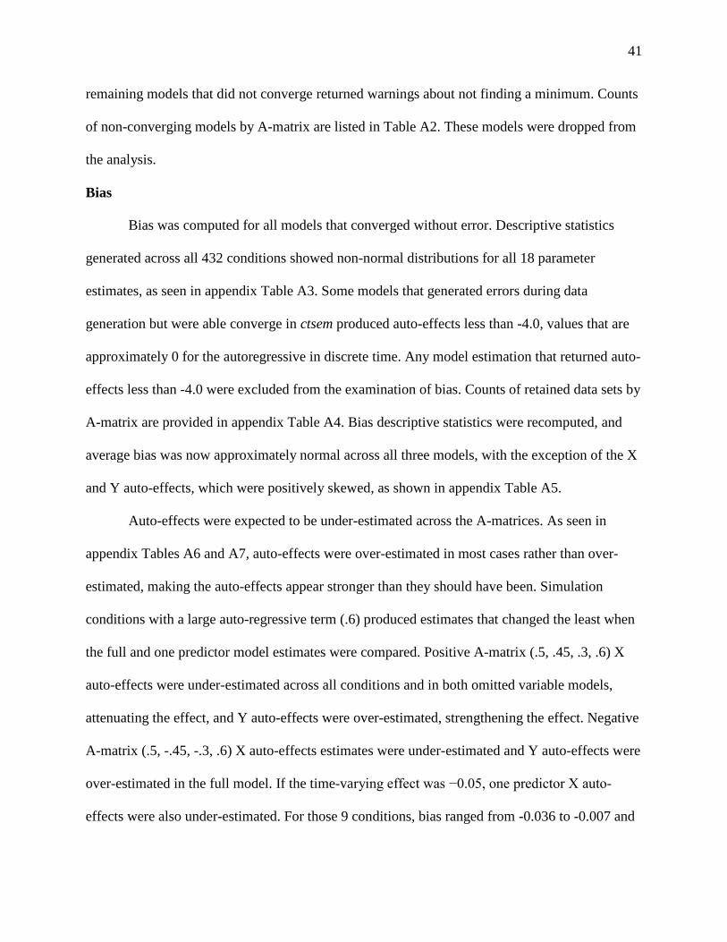
41

remaining models that did not converge returned warnings about not finding a minimum. Counts

of non-converging models by A-matrix are listed in Table A2. These models were dropped from

the analysis.

Bias

Bias was computed for all models that converged without error. Descriptive statistics

generated across all 432 conditions showed non-normal distributions for all 18 parameter

estimates, as seen in appendix Table A3. Some models that generated errors during data

generation but were able converge in ctsem produced auto-effects less than -4.0, values that are

approximately 0 for the autoregressive in discrete time. Any model estimation that returned auto-

effects less than -4.0 were excluded from the examination of bias. Counts of retained data sets by

A-matrix are provided in appendix Table A4. Bias descriptive statistics were recomputed, and

average bias was now approximately normal across all three models, with the exception of the X

and Y auto-effects, which were positively skewed, as shown in appendix Table A5.

Auto-effects were expected to be under-estimated across the A-matrices. As seen in

appendix Tables A6 and A7, auto-effects were over-estimated in most cases rather than over-

estimated, making the auto-effects appear stronger than they should have been. Simulation

conditions with a large auto-regressive term (.6) produced estimates that changed the least when

the full and one predictor model estimates were compared. Positive A-matrix (.5, .45, .3, .6) X

auto-effects were under-estimated across all conditions and in both omitted variable models,

attenuating the effect, and Y auto-effects were over-estimated, strengthening the effect. Negative

A-matrix (.5, -.45, -.3, .6) X auto-effects estimates were under-estimated and Y auto-effects were

over-estimated in the full model. If the time-varying effect was −0.05, one predictor X auto-

effects were also under-estimated. For those 9 conditions, bias ranged from -0.036 to -0.007 and

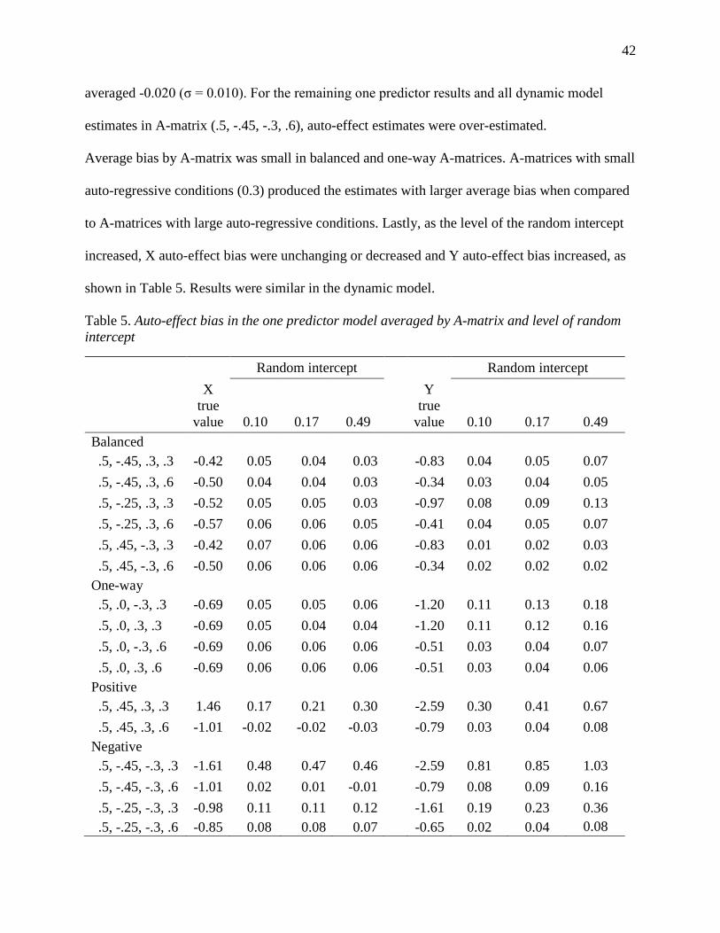
42

averaged -0.020 (σ = 0.010). For the remaining one predictor results and all dynamic model

estimates in A-matrix (.5, -.45, -.3, .6), auto-effect estimates were over-estimated.

Average bias by A-matrix was small in balanced and one-way A-matrices. A-matrices with small

auto-regressive conditions (0.3) produced the estimates with larger average bias when compared

to A-matrices with large auto-regressive conditions. Lastly, as the level of the random intercept

increased, X auto-effect bias were unchanging or decreased and Y auto-effect bias increased, as

shown in Table 5. Results were similar in the dynamic model.

Table 5. Auto-effect bias in the one predictor model averaged by A-matrix and level of random intercept

Random intercept Random intercept

X true

value 0.10 0.17 0.49

Y true

value 0.10 0.17 0.49 Balanced .5, -.45, .3, .3 -0.42 0.05 0.04 0.03 -0.83 0.04 0.05 0.07 .5, -.45, .3, .6 -0.50 0.04 0.04 0.03 -0.34 0.03 0.04 0.05 .5, -.25, .3, .3 -0.52 0.05 0.05 0.03 -0.97 0.08 0.09 0.13 .5, -.25, .3, .6 -0.57 0.06 0.06 0.05 -0.41 0.04 0.05 0.07 .5, .45, -.3, .3 -0.42 0.07 0.06 0.06 -0.83 0.01 0.02 0.03 .5, .45, -.3, .6 -0.50 0.06 0.06 0.06 -0.34 0.02 0.02 0.02 One-way .5, .0, -.3, .3 -0.69 0.05 0.05 0.06 -1.20 0.11 0.13 0.18 .5, .0, .3, .3 -0.69 0.05 0.04 0.04 -1.20 0.11 0.12 0.16 .5, .0, -.3, .6 -0.69 0.06 0.06 0.06 -0.51 0.03 0.04 0.07 .5, .0, .3, .6 -0.69 0.06 0.06 0.06 -0.51 0.03 0.04 0.06 Positive .5, .45, .3, .3 1.46 0.17 0.21 0.30 -2.59 0.30 0.41 0.67 .5, .45, .3, .6 -1.01 -0.02 -0.02 -0.03 -0.79 0.03 0.04 0.08 Negative .5, -.45, -.3, .3 -1.61 0.48 0.47 0.46 -2.59 0.81 0.85 1.03 .5, -.45, -.3, .6 -1.01 0.02 0.01 -0.01 -0.79 0.08 0.09 0.16 .5, -.25, -.3, .3 -0.98 0.11 0.11 0.12 -1.61 0.19 0.23 0.36 .5, -.25, -.3, .6 -0.85 0.08 0.08 0.07 -0.65 0.02 0.04 0.08

43

Expectations about cross-effect estimates were based on simulation conditions for

the cross-lag. If the cross-lag condition was negative, the estimates would be biased but no

direction was specified. If the cross-lag condition was positive, it was hypothesized that the

estimates would be over-estimated. Balanced A-matrix cross-effects were minimally biased as

indicated in the average bias of cross-effects in appendix Tables A8 and A9. One-way A-

matrices produced unbiased or positively biased estimates if the non-zero cross-lag condition

was negative, but only one of the two cross-effects was negatively biased if the non-zero cross-

lag condition was positive. Cross-effects in positive A-matrices were negatively biased, and

positively biased in negative A-matrix conditions, results that indicated attenuated estimates. In

the comparison of bias between the full and omitted variable models by taking the difference, the

influence of the omitted variables on estimation appeared to be largest in the dynamic model

with very few A-matrix averages not changing. If the data was generated with a large auto-

regressive conditions or with a balanced or one-way A-matrix, the change in bias from full to the

one predictor model was minimal, and in a few instances, less in the one predictor model.

Bias in the time-invariant effects for the predictor retained in the one predictor model was

expected to depend on the time-invariant correlation in negative cross-lag conditions. Negative

cross-lag conditions were equally biased across the levels of the time-invariant correlations with

no consistent differences identified across type of A-matrix. Figure 6 shows results by time-

invariant correlation for the balanced A-matrices, bias patterns that were not unique to that type

of A-matrix. Bias was predicted in the positive cross-lag condition but not dependent on any

other condition, and results were all biased in those conditions with estimates that were

attenuated. Balanced A-matrices appeared to change the least, specifically those with a large

auto-regressive term.

44

Figure 6. Bias of time-invariant effects on trait variance. Results are for balanced A-matrices at each level of the time-invariant correlation between the two time-invariant predictors in the data generation model.

Overall, bias of estimates followed patterns different than what was hypothesized. The

estimates in negative A-matrices were the most biased. Cross-lag conditions and other simulation

conditions influenced results, but in some instances, bias did not change as variables were

omitted, particularly conditions with a large auto-regressive simulation condition. Results that

explore bias across models for the same condition follow in the sections below where relative

bias and relative efficiency are presented.

Effects of omitted variables

In order to determine whether estimates from the exact discrete model were robust to

omitted variable variance, both relative bias and efficiency were calculated. Relative bias and

efficiency of the dynamic process were computed twice, for the full model versus the one

predictor model, and for the full model versus the dynamic model. Time-invariant estimates were

estimated in two of the three models so relative ratios were computed once for that part of the

-0.40-0.35-0.30-0.25-0.20-0.15-0.10-0.050.00

-0.3 0 0.3

Bias

Time-invariant correlation

X trait variance

.5, -.45, .3, .3 .5, -.45, .3, .6

.5, -.25, .3, .3 .5, -.25, .3, .6

.5, .45, -.3, .3 .5, .45, -.3, .6

-0.40-0.35-0.30-0.25-0.20-0.15-0.10-0.050.00

-0.3 0 0.3

Bias

Time-invariant correlation

Y trait variance

.5, -.45, .3, .3 .5, -.45, .3, .6

.5, -.25, .3, .3 .5, -.25, .3, .6

.5, .45, -.3, .3 .5, .45, -.3, .6

45

analysis. The full model was estimated according to the data generation model, the one predictor

model dropped one time-invariant predictor, and the dynamic model dropped all predictors.

Relative bias and relative efficiency were computed for model results with and without

outliers. Even after excluding problematic estimations based on the X auto-effect < ‑4.0, the

results still contained some relative bias or efficiency values that acted as outliers in the analysis,

particularly in the results for the estimates of time-invariant effects on trait variance. Any time

extremely large relative bias and relative efficiency results were obtained, the original bias

estimates were examined to see if a small amount of bias in one model, such as 0.005 or smaller,

was responsible for the result.

Both ratios used the full model in the numerator and the omitted variable models in the

denominator for two bias ratios and two efficiency ratios. Ratios close to 1.00, plus or minus .10,

indicate that bias or efficiency was equal in the two models. Ratios above 1.10 indicate the

omitted variable model was less biased or more efficient with ratios below .90 indicate that the

full model was less biased or more efficient. The bias results are presented first by type of

parameter estimates, auto-effect, cross-effect, and time-invariant estimate. Within each

parameter type, type of A-matrix was used to organize the sections in the following order:

balanced, one-way, positive, and negative. Organized in the same way, relative efficiency results

follow.

Relative bias

Auto-effects. Figure 7 shows a common pattern in auto-effect relative bias across A-

matrices. If the time-invariant effect was −0.05, bias was equal in the full and one predictor

models. If the time-varying effects were ±0.30, three of the four negative A-matrices and all one-

way A-matrices produced auto-effects that were less biased in the full model. Dynamic auto-

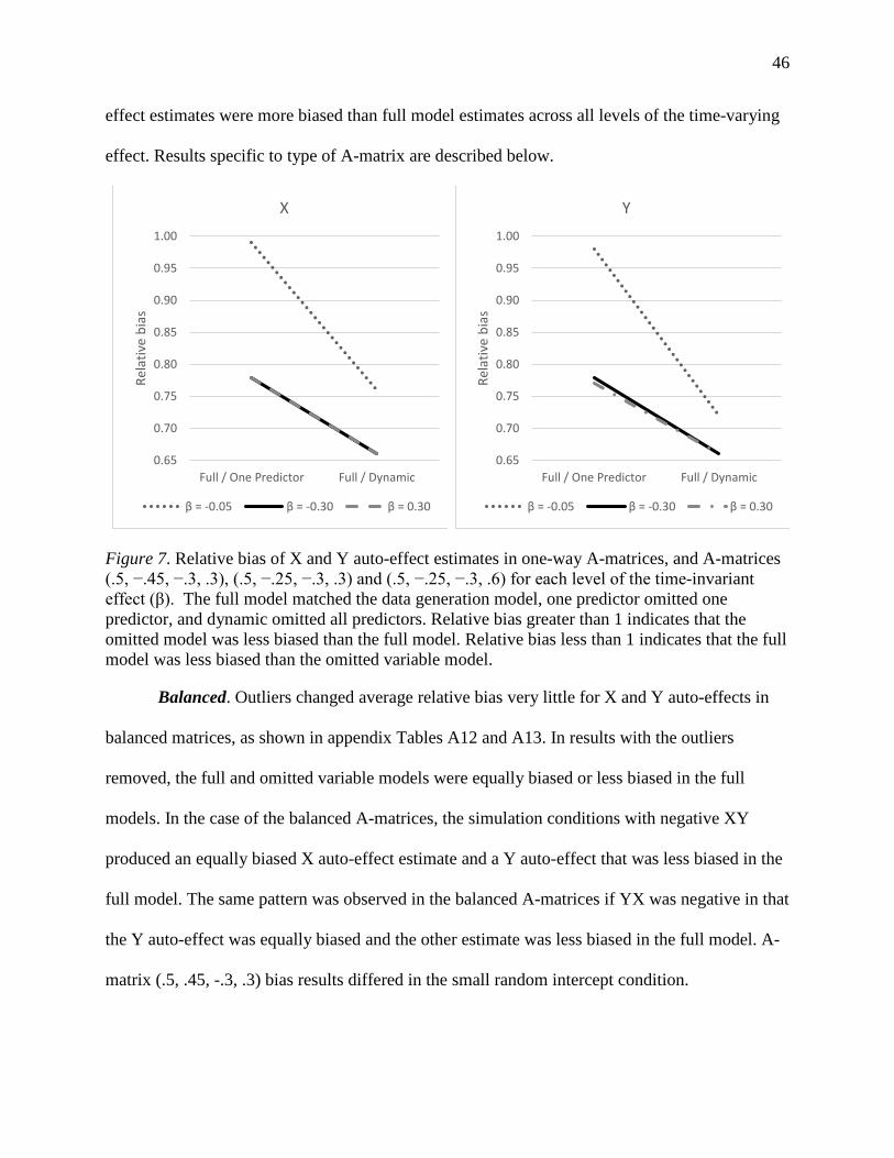
46

effect estimates were more biased than full model estimates across all levels of the time-varying

effect. Results specific to type of A-matrix are described below.

Figure 7. Relative bias of X and Y auto-effect estimates in one-way A-matrices, and A-matrices (.5, −.45, −.3, .3), (.5, −.25, −.3, .3) and (.5, −.25, −.3, .6) for each level of the time-invariant effect (β). The full model matched the data generation model, one predictor omitted one predictor, and dynamic omitted all predictors. Relative bias greater than 1 indicates that the omitted model was less biased than the full model. Relative bias less than 1 indicates that the full model was less biased than the omitted variable model.

Balanced. Outliers changed average relative bias very little for X and Y auto-effects in

balanced matrices, as shown in appendix Tables A12 and A13. In results with the outliers

removed, the full and omitted variable models were equally biased or less biased in the full

models. In the case of the balanced A-matrices, the simulation conditions with negative XY

produced an equally biased X auto-effect estimate and a Y auto-effect that was less biased in the

full model. The same pattern was observed in the balanced A-matrices if YX was negative in that

the Y auto-effect was equally biased and the other estimate was less biased in the full model. A-

matrix (.5, .45, -.3, .3) bias results differed in the small random intercept condition.

0.65

0.70

0.75

0.80

0.85

0.90

0.95

1.00

Full / One Predictor Full / Dynamic

Rela

tive

bias

X

β = -0.05 β = -0.30 β = 0.30

0.65

0.70

0.75

0.80

0.85

0.90

0.95

1.00

Full / One Predictor Full / DynamicRe

lativ

e bi

as

Y

β = -0.05 β = -0.30 β = 0.30

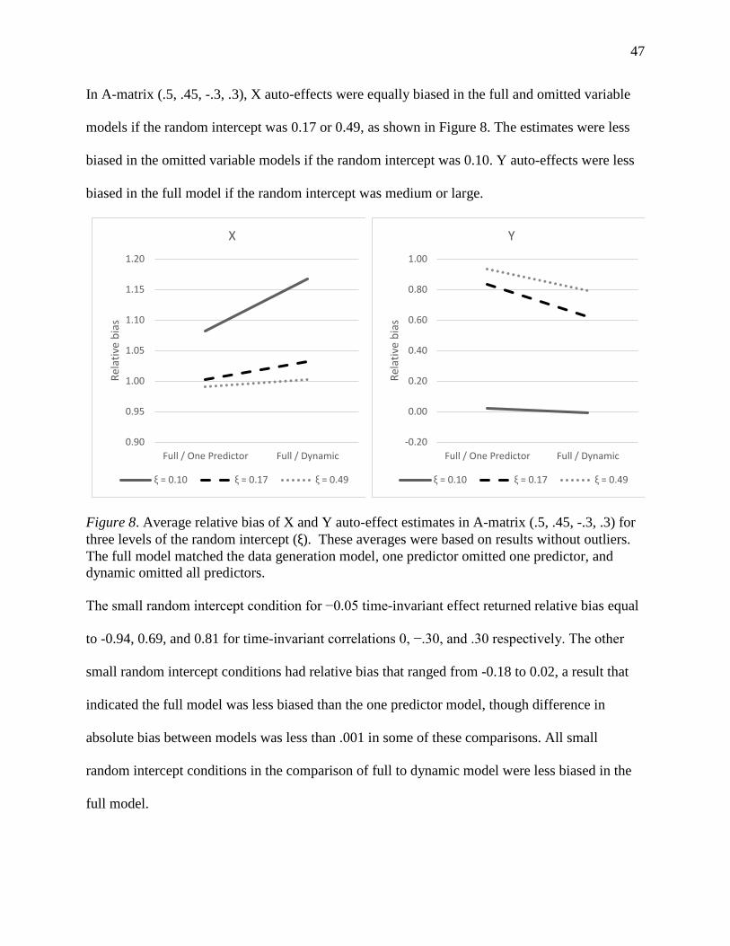
47

In A-matrix (.5, .45, -.3, .3), X auto-effects were equally biased in the full and omitted variable

models if the random intercept was 0.17 or 0.49, as shown in Figure 8. The estimates were less

biased in the omitted variable models if the random intercept was 0.10. Y auto-effects were less

biased in the full model if the random intercept was medium or large.

Figure 8. Average relative bias of X and Y auto-effect estimates in A-matrix (.5, .45, -.3, .3) for three levels of the random intercept (ξ). These averages were based on results without outliers. The full model matched the data generation model, one predictor omitted one predictor, and dynamic omitted all predictors. The small random intercept condition for −0.05 time-invariant effect returned relative bias equal

to -0.94, 0.69, and 0.81 for time-invariant correlations 0, −.30, and .30 respectively. The other

small random intercept conditions had relative bias that ranged from -0.18 to 0.02, a result that

indicated the full model was less biased than the one predictor model, though difference in

absolute bias between models was less than .001 in some of these comparisons. All small

random intercept conditions in the comparison of full to dynamic model were less biased in the

full model.

0.90

0.95

1.00

1.05

1.10

1.15

1.20

Full / One Predictor Full / Dynamic

Rela

tive

bias

X

ξ = 0.10 ξ = 0.17 ξ = 0.49

-0.20

0.00

0.20

0.40

0.60

0.80

1.00

Full / One Predictor Full / Dynamic

Rela

tive

bias

Y

ξ = 0.10 ξ = 0.17 ξ = 0.49

48

One-way. Outliers had little effect on average relative bias in the three of the four one-

way A-matrices, as indicated in appendix Tables A12 and A13. A-matrix (.5, 0, .3, .3) contained

a single condition that averaged -52.89 for relative bias of the Y auto-effect across replications.

After removal of outliers, whether the full and one predictor models were equally biased or the

full model was less biased depended on the size of the time-invariant effect, as described at the

beginning of the section.

Positive. Relative bias results differed for the two positive A-matrices. The positive A-

matrix with small auto-regressive term was equally biased in the comparison of full model to one

predictor except in conditions with time-invariant effect of ±0.30 with small random intercept, in

which case one auto-effect was equally biased and the other was less biased in the full model. In

the dynamic model, aside from the −0.05 time-invariant effect condition, the only conditions that

were equally biased were those with a large random intercept, as shown in Figure 9.

Figure 9. Average relative bias of Y auto-effect estimates in positive A-matrices for three levels of the random intercept (ξ). These averages were based on results without outliers. The full model matched the data generation model, one predictor omitted one predictor, and dynamic omitted all predictors.

0.70

0.75

0.80

0.85

0.90

0.95

1.00

1.05

1.10

1.15

1.20

Full / One predictor Full / Dynamic

Rela

tive

bias

A-matrix (.5, .45, .3, .3)

ξ = 0.10 ξ = 0.17 ξ = 0.49

0.70

0.75

0.80

0.85

0.90

0.95

1.00

1.05

1.10

1.15

1.20

Full / One predictor Full / Dynamic

Rela

tive

bias

A-matrix (.5, .45, .3, .6)

ξ = 0.10 ξ = 0.17 ξ = 0.49

49

A-matrix (.5, .45, .3, .6) relative bias results for X auto-effects, were equally biased or

less biased in the full to one predictor model comparison. With the omission of all predictors,

relative bias decreased in all but condition. That condition was 0.10 random intercept, .30 time-

invariant correlation, and −0.30 time-invariant effect, and relative bias ranged from 0.96 to 1.02,

which still indicated equal bias. In that same condition, relative bias for the Y auto-effect

decreased as more predictors were omitted, going from 1.19 to 1.04. For 22 of the other

conditions in which relative bias for X auto-effect decreased as more variables were omitted,

results for Y auto-effects were the exact opposite. The remaining four conditions produced both

X and Y auto-effect estimates that were less in the full to dynamic model comparison than in the

full to one predictor model comparison.

Negative. Negative A-matrix estimates were impacted the most by outliers. Averages by

A-matrix, both with and without outliers, are listed in appendix Tables A12 and A13. Even after

the removal of outlier auto-effect estimates, relative bias equaled -4.65 in A-matrix (.5, -.45, -.3,

.6) for X auto-effects in the comparison of the full to the one predictor model. One predictor

model results were less biased in conditions with 0.49 random intercept and time-varying effects

−0.30 and 0.30. Results for individual simulation conditions without outliers were similar to the

other negative A-matrices, relative bias that differed by level of time-invariant effect as in one-

way and balanced A-matrices.

For X auto-effects in A-matrix (.5, -.45, -.3, .6), relative bias was negative if the time-

invariant effect was −0.30 or 0.30 in the comparison between the full and one predictor model

and for every condition in the full versus dynamic model comparisons. Relative bias also

differed by level of the random intercept, as shown in Figure 10. Examination of bias values for

the condition with time-varying effect 0.3 and random intercept 0.49 showed bias of -0.0389 and

50

0.0004 in the full and one predictor models respectively. That translated to -90.98 for the relative

bias for that one condition. Relative bias results appeared extremely large, but the small amount

of bias made it look exceptionally large.

Figure 10. Relative bias of X auto-effect estimates in A-matrix (.5, -.45, -.3, .6) by random intercept (ξ) and level of the time-invariant effect (β). These averages were based on results without outliers. The full model matched the data generation model, one predictor omitted one predictor, and dynamic omitted all predictors.

Cross-effects. Only in conditions with −0.05 time-varying effect were the full and one

predictor model equally biased. Removal of outliers based on unrealistic auto-effects removed

cases in which there appeared to be a difference between models. Results averaged across A-

matrix are listed for the four cross-lag types in appendix Tables A14 and A15.

Balanced. Cross-effect bias in balanced A-matrices differed little between the full and

omitted variable models with average bias by A-matrix being equal and near 0, as shown in

appendix Tables A7 and A8. For example, in A-matrix (.5, -.45, .3, .3) the largest absolute

difference in YX bias between the full and one predictor estimates was 0.0027. With such small

differences in bias, the relative bias results depended upon differences in the one-hundredth

-0.50

-0.30

-0.10

0.10

0.30

0.50

0.70

0.90

1.10

Full / One Predictor Full / Dynamic

Rela

tive

bias

ξ is 0.10 or 0.17

β = -0.05 β = -0.30 β = 0.30

-42.00

-37.00

-32.00

-27.00

-22.00

-17.00

-12.00

-7.00

-2.00

3.00

Full / One Predictor Full / Dynamic

Rela

tive

bias

ξ is 0.49

β = -0.05 β = -0.30 β = 0.30

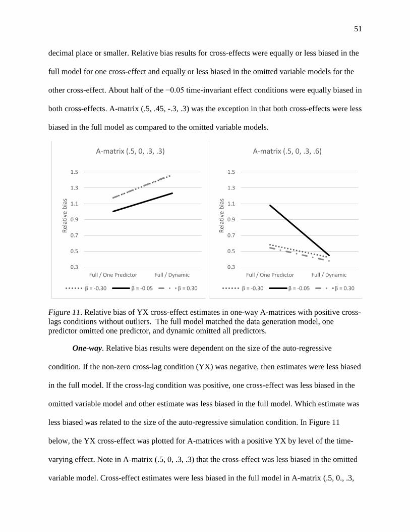
51

decimal place or smaller. Relative bias results for cross-effects were equally or less biased in the

full model for one cross-effect and equally or less biased in the omitted variable models for the

other cross-effect. About half of the −0.05 time-invariant effect conditions were equally biased in

both cross-effects. A-matrix (.5, .45, -.3, .3) was the exception in that both cross-effects were less

biased in the full model as compared to the omitted variable models.

Figure 11. Relative bias of YX cross-effect estimates in one-way A-matrices with positive cross-lags conditions without outliers. The full model matched the data generation model, one predictor omitted one predictor, and dynamic omitted all predictors.

One-way. Relative bias results were dependent on the size of the auto-regressive

condition. If the non-zero cross-lag condition (YX) was negative, then estimates were less biased

in the full model. If the cross-lag condition was positive, one cross-effect was less biased in the

omitted variable model and other estimate was less biased in the full model. Which estimate was

less biased was related to the size of the auto-regressive simulation condition. In Figure 11

below, the YX cross-effect was plotted for A-matrices with a positive YX by level of the time-

varying effect. Note in A-matrix (.5, 0, .3, .3) that the cross-effect was less biased in the omitted

variable model. Cross-effect estimates were less biased in the full model in A-matrix (.5, 0., .3,

0.3

0.5

0.7

0.9

1.1

1.3

1.5

Full / One Predictor Full / Dynamic

Rela

tive

bias

A-matrix (.5, 0, .3, .3)

β = -0.30 β = -0.05 β = 0.30

0.3

0.5

0.7

0.9

1.1

1.3

1.5

Full / One Predictor Full / Dynamic

Rela

tive

bias

A-matrix (.5, 0, .3, .6)

β = -0.30 β = -0.05 β = 0.30

52

.6) for time-varying effects −0.30 and 0.30. In those A-matrices, XY cross-effect bias was the

mirror image of the YX results.

YX Cross-effect XY Cross-effect

Figure 12. Relative bias of YX and XY cross-effect estimates in A-matrices with positive cross-lags for each level of the time-invariant effect (β). These averages were based on results without outliers. The full model matched the data generation model, one predictor omitted one predictor, and dynamic omitted all predictors.

0.75

0.80

0.85

0.90

0.95

1.00

1.05

1.10

1.15

Full / One Predictor Full / Dynamic

Rela

tive

bias

ξ is .10, .17

β = -0.30 β = -0.05 β = 0.30

0.75

0.80

0.85

0.90

0.95

1.00

1.05

1.10

1.15

Full / One Predictor Full / Dynamic

Rela

tive

bias

ξ is .10, .17

β = -0.30 β = -0.05 β = 0.30

0.75

0.80

0.85

0.90

0.95

1.00

1.05

1.10

1.15

Full / One Predictor Full / Dynamic

Rela

tive

bias

ξ is .49

β = -0.30 β = -0.05 β = 0.30

0.75

0.80

0.85

0.90

0.95

1.00

1.05

1.10

1.15

Full / One Predictor Full / Dynamic

Rela

tive

bias

ξ is .49

β = -0.30 β = -0.05 β = 0.30

53

Positive. Relative bias for positive A-matrix (.5, .45, .3, .6) conditions was near 1, which

indicated equal bias in the full and omitted variable models. Results varied in A-matrix (.5, .45,

.3, .3) across conditions. The results from the full to one predictor model comparison indicated

equal bias if the random intercept was 0.49, though YX was less biased in the omitted variable

models if the time-varying effect was not −0.05. If the random intercept was 0.10 or 0.17, then

both cross-effects were equally biased in the full to one predictor comparison. In the full to

dynamic model comparison, YX was less biased in the dynamic model and XY was less biased

in the full model. Relative bias averaged over random intercepts and time-varying effects in A-

matrix (.5, .45, .3, .3) were plotted in Figure 12.

Negative. Aside from A-matrix conditions, simulation conditions had little impact on

negative A-matrices. The only conditions that produced estimates that were equally biased was if

the time-invariant effect was −0.05 in the comparison of the full to the one predictor model.

Otherwise, both estimates were less biased in the full model. All estimates were less biased in the

full model when compared to the dynamic model.

Time-invariant predictor. Outliers in time-invariant effects on trait variance affected

results for negative A-matrix (.5, -.45, -.3, .3) the most. There were many conditions in which the

time-invariant effect was −0.30 or 0.30 that relative bias indicated less bias in the one predictor

model, but removal of outliers resulted in relative bias less than 1, results that indicated the full

model was less biased. As shown in appendix Tables A16 and A17, other A-matrix conditions

contained results with outliers that influenced relative bias, but removal of outliers reduced the

degree of bias but did not change the conclusion.

In all A-matrices, simulation conditions with −0.05 time-invariant effects and 0 time-

invariant correlation was 0 were equally biased in the models. Some other conditions were

54

equally biased, but the exact set of conditions varied by A-matrix type. In many conditions, pairs

of time-invariant effect and time-invariant correlation determined whether estimates were

equally biased or not. More specifically, whether conditions were both positive, both negative, or

opposite in sign determined results in conjunction with A-matrix type.

Balanced. Regardless of level of simulated time-invariant effect condition, if the time-

invariant correlation was 0, both effects on trait variance estimates were equally biased. In the

other conditions, one time-invariant effect on trait variance was equally biased and the other was

less biased in one model. The effect on X trait variance was equal if XY was positive, except in

A-matrix (.5, .45, -.3, .3), in which the estimate was less biased in the one predictor model.

Likewise, the effect on Y trait variance was equal if YX was positive. The other estimate was

less biased in the one predictor model if time-invariant effects and correlation were both negative

or both positive. If one was positive and the other was negative, the other estimate was less

biased in the full model. Averages by combination of simulation conditions are listed in Table 6.

Table 6. Relative bias for time-invariant effects on X and Y trait variance by balanced A-matrix and combination of time-invariant correlation (r) and effect (β) simulation conditions

(.5, .45, -.3, .6) (.5, .45, -.3, .3) All other A Simulation conditions for r / β

X trait variance

Y trait variance

X trait variance

Y trait variance

X trait variance

Y trait variance

r = 0 0 / −0.05 1.00 1.00 1.00 1.00 1.00 1.00 0 / −0.30 0.99 0.95 1.00 0.98 0.95 1.00 0 / 0.30 0.99 0.96 1.00 0.98 0.95 1.00 Opposite sign

.30 / −0.05 1.02 0.87 1.01 0.95 0.89 1.00 -.3 / 0.3 1.15 0.53 1.08 0.75 0.57 0.99 .30 / −0.30 1.16 0.52 1.08 0.75 0.57 0.99

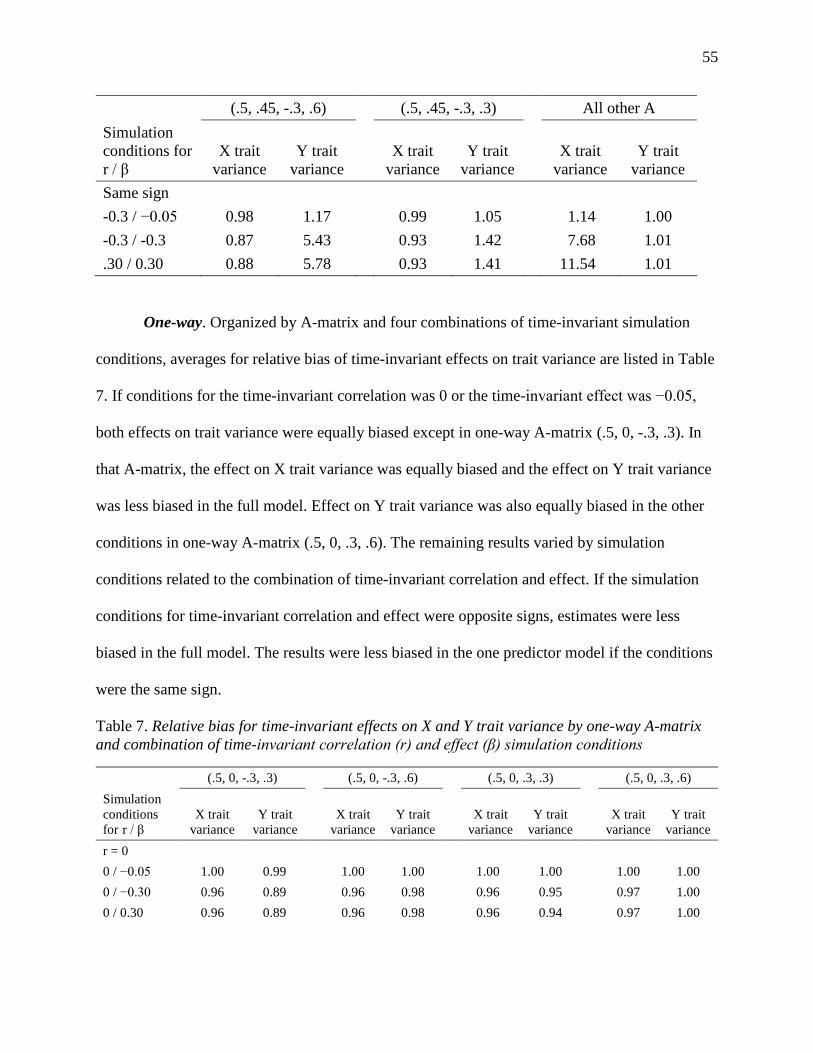
55

(.5, .45, -.3, .6) (.5, .45, -.3, .3) All other A Simulation conditions for r / β

X trait variance

Y trait variance

X trait variance

Y trait variance

X trait variance

Y trait variance

Same sign

-0.3 / −0.05 0.98 1.17 0.99 1.05 1.14 1.00 -0.3 / -0.3 0.87 5.43 0.93 1.42 7.68 1.01 .30 / 0.30 0.88 5.78 0.93 1.41 11.54 1.01

One-way. Organized by A-matrix and four combinations of time-invariant simulation

conditions, averages for relative bias of time-invariant effects on trait variance are listed in Table

7. If conditions for the time-invariant correlation was 0 or the time-invariant effect was −0.05,

both effects on trait variance were equally biased except in one-way A-matrix (.5, 0, -.3, .3). In

that A-matrix, the effect on X trait variance was equally biased and the effect on Y trait variance

was less biased in the full model. Effect on Y trait variance was also equally biased in the other

conditions in one-way A-matrix (.5, 0, .3, .6). The remaining results varied by simulation

conditions related to the combination of time-invariant correlation and effect. If the simulation

conditions for time-invariant correlation and effect were opposite signs, estimates were less

biased in the full model. The results were less biased in the one predictor model if the conditions

were the same sign.

Table 7. Relative bias for time-invariant effects on X and Y trait variance by one-way A-matrix and combination of time-invariant correlation (r) and effect (β) simulation conditions

(.5, 0, -.3, .3) (.5, 0, -.3, .6) (.5, 0, .3, .3) (.5, 0, .3, .6) Simulation conditions for r / β

X trait variance

Y trait variance

X trait variance

Y trait variance

X trait variance

Y trait variance

X trait variance

Y trait variance

r = 0 0 / −0.05 1.00 0.99 1.00 1.00 1.00 1.00 1.00 1.00 0 / −0.30 0.96 0.89 0.96 0.98 0.96 0.95 0.97 1.00 0 / 0.30 0.96 0.89 0.96 0.98 0.96 0.94 0.97 1.00

56

(.5, 0, -.3, .3) (.5, 0, -.3, .6) (.5, 0, .3, .3) (.5, 0, .3, .6) Simulation conditions for r / β

X trait variance

Y trait variance

X trait variance

Y trait variance

X trait variance

Y trait variance

X trait variance

Y trait variance

Opposite sign .30 / −0.05 0.96 0.85 0.96 0.98 0.96 0.93 0.95 1.00 −.30 / 0.30 0.78 0.48 0.77 0.89 0.79 0.69 0.75 1.02 .30 / −0.30 0.78 0.48 0.77 0.89 0.79 0.69 0.76 1.02 Same sign −.30 / −0.05 1.04 1.20 1.05 1.02 1.04 1.07 1.05 1.00 −.30 / −0.30 1.26 9.97 1.28 1.10 1.24 1.51 1.37 0.98 .30 / 0.30 1.25 8.95 1.29 1.10 1.24 1.52 1.37 0.98

Positive. Positive A-matrix (.5, .45, .3, .6) estimates of effects on trait variance were

equally biased in all conditions. Results for A-matrix (.5, .45, .3, .3) were similar to one-way A-

matrices. If the time-invariant effect was −0.05 or the time-invariant correlation was 0, both

estimates were equally biased in the full and one predictor model. For same sign pairs, the effect

on X trait variance was less biased in the full model with an average of 0.90, and the effect on Y

trait variance was less biased in the one predictor model with an average of 1.38. For opposite

sign pairs, the relative bias pattern was reversed. The effect on X trait variance was less biased in

the one predictor model with an average of 1.19, and the effect on Y trait variance was less

biased in the full model with an average of 0.73.

Negative. Average relative bias by the combination of time-invariant simulation

conditions are listed in Table 8. Only conditions with 0, −0.05 conditions for time-invariant

correlation (r) and effect (β) respectively were equally biased across the negative A-matrices.

Estimates were less biased in the full model for the other 0 time-invariant correlation conditions

and conditions in which pairs of time-invariant correlations and effects were opposite in sign. If

the pairs were the same sign, the one predictor model was less biased. Note, in the table below in

57

A-matrix (.5, -.45, -.3, .6) that the average bias was -0.96 if the simulation conditions were -.3

time-invariant correlation and −0.30 time-invariant effect. In this A-matrix, random intercept

values of 0.10, 0.17, and 0.49 had relative bias of -23.68, 15.72, and 5.08 respectively. Bias

results showed average bias in the full model was -0.122, -0.136, and -0.158 for the three random

intercept levels. In the one predictor model, average bias was -0.005, - 0.009, and -0.031 so the

one predictor model was able to produce less biased estimates of time-invariant effects on trait

variance in this set of simulation conditions.

Table 8. Relative bias for time-invariant effects on X and Y trait variance by negative A-matrix and combination of time-invariant correlation (r) and effect (β) simulation conditions

(.5,-.45, -.3, .3) (.5, -.45, -.3, .6) (.5, -.25, -.3, .3) (.5, -.25, -.3, .6) Simulation conditions for r / β

X trait variance

Y trait variance

X trait variance

Y trait variance

X trait variance

Y trait variance

X trait variance

Y trait variance

r = 0 0 / −0.05 1.00 1.00 0.99 1.00 0.99 0.99 1.00 1.00 0 / −0.30 0.89 0.90 0.84 0.90 0.83 0.81 0.93 0.94 0 / 0.30 0.89 0.90 0.83 0.90 0.82 0.81 0.93 0.94 Opposite sign .30 / −0.05 0.91 0.92 0.84 0.92 0.87 0.85 0.91 0.93 −.30 / 0.30 0.60 0.63 0.43 0.62 0.50 0.46 0.62 0.67 .30 / −0.30 0.61 0.64 0.44 0.62 0.50 0.47 0.62 0.67 Same sign −.30 / −0.05 1.10 1.09 1.23 1.09 1.15 1.19 1.10 1.08 −.30 / −0.30 1.77 1.63 -0.96 1.68 2.59 4.29 1.90 1.60 .30 / 0.30 1.72 1.60 12.31 1.66 2.54 4.17 1.90 1.61

Relative efficiency

After relative bias was computed, relative efficiency, a formula that takes into account

bias and variability, was calculated. Tables with relative efficiency averaged by A-matrix can be

found in Appendix A, Tables A17 – A21. Efficiency 1.00 ± 0.10 indicates that the full model and

the omitted variable model were equally efficient. The full model is more efficient if relative

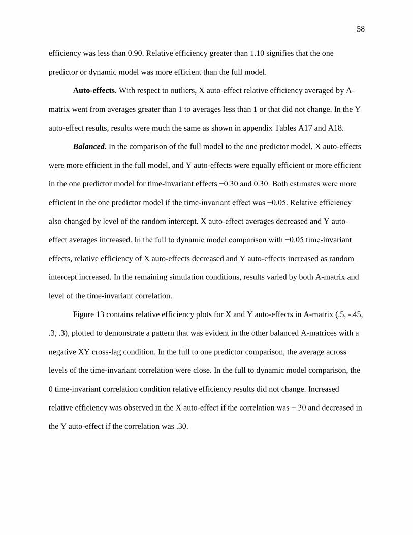
58

efficiency was less than 0.90. Relative efficiency greater than 1.10 signifies that the one

predictor or dynamic model was more efficient than the full model.

Auto-effects. With respect to outliers, X auto-effect relative efficiency averaged by A-

matrix went from averages greater than 1 to averages less than 1 or that did not change. In the Y

auto-effect results, results were much the same as shown in appendix Tables A17 and A18.

Balanced. In the comparison of the full model to the one predictor model, X auto-effects

were more efficient in the full model, and Y auto-effects were equally efficient or more efficient

in the one predictor model for time-invariant effects −0.30 and 0.30. Both estimates were more

efficient in the one predictor model if the time-invariant effect was −0.05. Relative efficiency

also changed by level of the random intercept. X auto-effect averages decreased and Y auto-

effect averages increased. In the full to dynamic model comparison with −0.05 time-invariant

effects, relative efficiency of X auto-effects decreased and Y auto-effects increased as random

intercept increased. In the remaining simulation conditions, results varied by both A-matrix and

level of the time-invariant correlation.

Figure 13 contains relative efficiency plots for X and Y auto-effects in A-matrix (.5, -.45,

.3, .3), plotted to demonstrate a pattern that was evident in the other balanced A-matrices with a

negative XY cross-lag condition. In the full to one predictor comparison, the average across

levels of the time-invariant correlation were close. In the full to dynamic model comparison, the

0 time-invariant correlation condition relative efficiency results did not change. Increased

relative efficiency was observed in the X auto-effect if the correlation was −.30 and decreased in

the Y auto-effect if the correlation was .30.

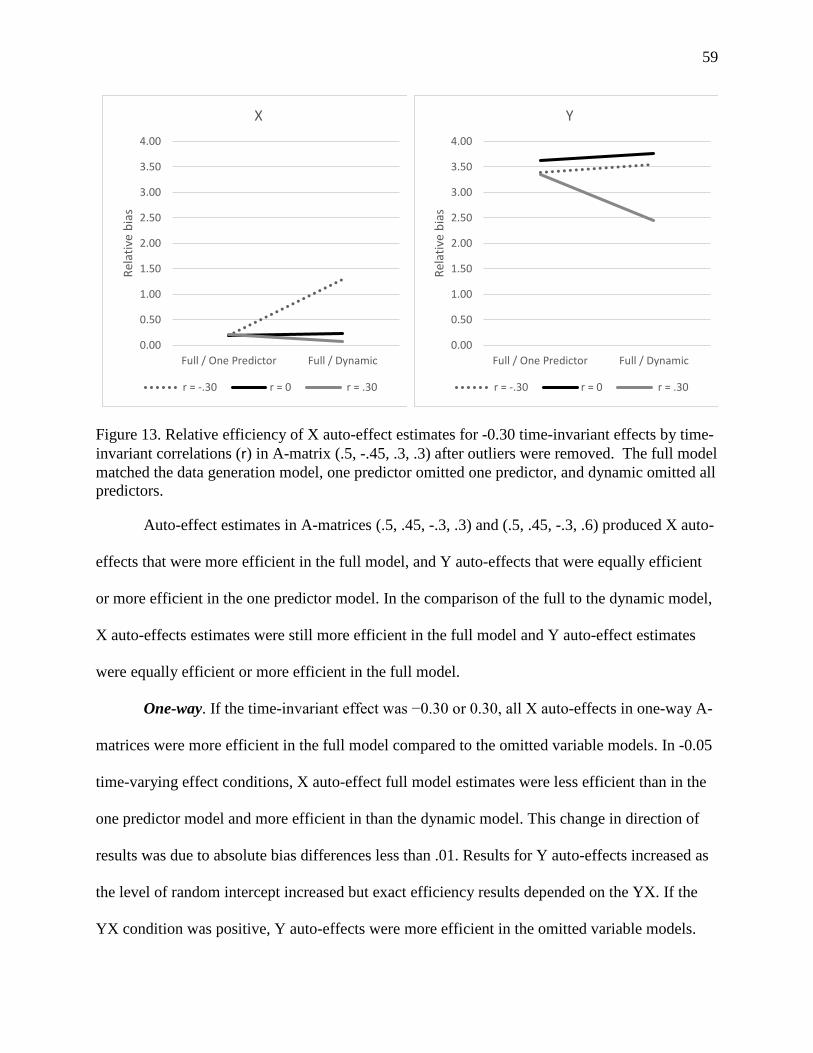
59

Figure 13. Relative efficiency of X auto-effect estimates for -0.30 time-invariant effects by time-invariant correlations (r) in A-matrix (.5, -.45, .3, .3) after outliers were removed. The full model matched the data generation model, one predictor omitted one predictor, and dynamic omitted all predictors.

Auto-effect estimates in A-matrices (.5, .45, -.3, .3) and (.5, .45, -.3, .6) produced X auto-

effects that were more efficient in the full model, and Y auto-effects that were equally efficient

or more efficient in the one predictor model. In the comparison of the full to the dynamic model,

X auto-effects estimates were still more efficient in the full model and Y auto-effect estimates

were equally efficient or more efficient in the full model.

One-way. If the time-invariant effect was −0.30 or 0.30, all X auto-effects in one-way A-

matrices were more efficient in the full model compared to the omitted variable models. In -0.05

time-varying effect conditions, X auto-effect full model estimates were less efficient than in the

one predictor model and more efficient in than the dynamic model. This change in direction of

results was due to absolute bias differences less than .01. Results for Y auto-effects increased as

the level of random intercept increased but exact efficiency results depended on the YX. If the

YX condition was positive, Y auto-effects were more efficient in the omitted variable models.

0.00

0.50

1.00

1.50

2.00

2.50

3.00

3.50

4.00

Full / One Predictor Full / Dynamic

Rela

tive

bias

X

r = -.30 r = 0 r = .30

0.00

0.50

1.00

1.50

2.00

2.50

3.00

3.50

4.00

Full / One Predictor Full / Dynamic

Rela

tive

bias

Y

r = -.30 r = 0 r = .30

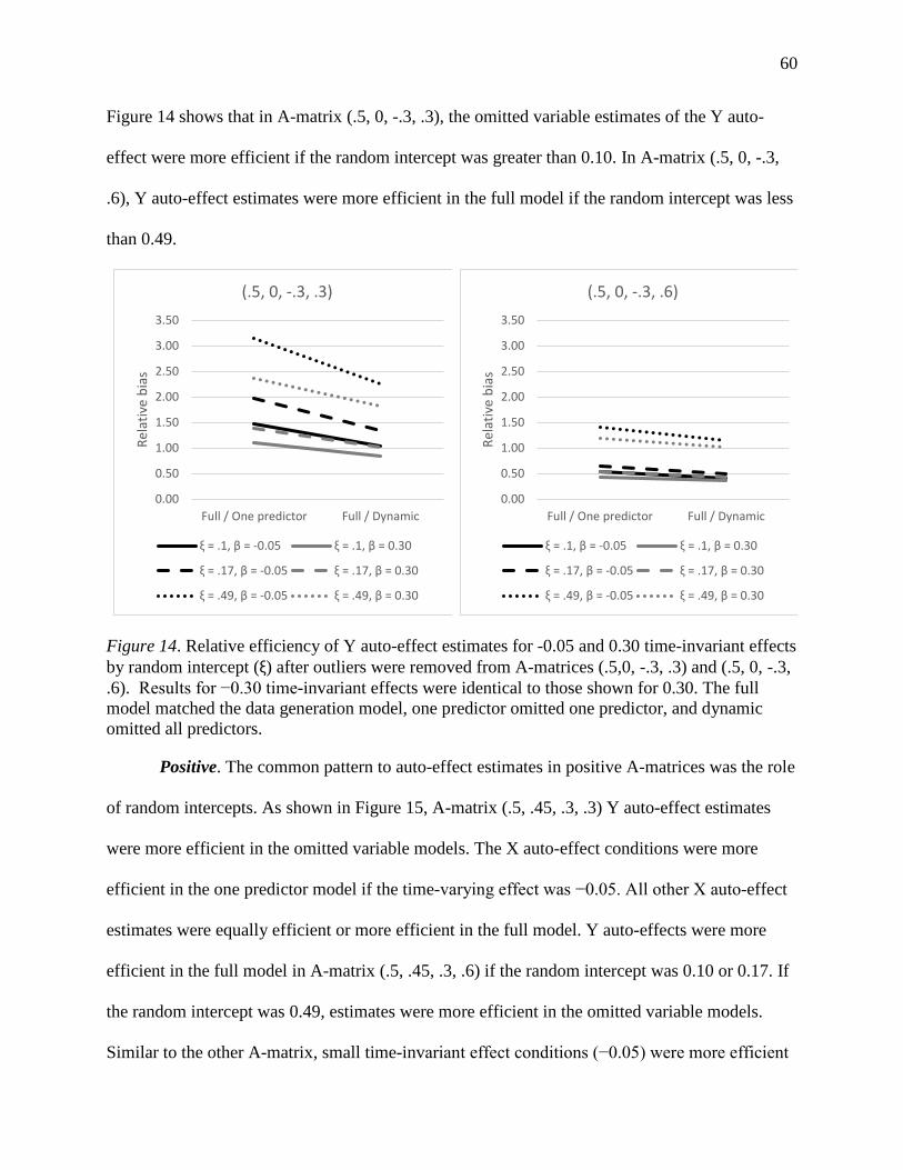
60

Figure 14 shows that in A-matrix (.5, 0, -.3, .3), the omitted variable estimates of the Y auto-

effect were more efficient if the random intercept was greater than 0.10. In A-matrix (.5, 0, -.3,

.6), Y auto-effect estimates were more efficient in the full model if the random intercept was less

than 0.49.

Figure 14. Relative efficiency of Y auto-effect estimates for -0.05 and 0.30 time-invariant effects by random intercept (ξ) after outliers were removed from A-matrices (.5,0, -.3, .3) and (.5, 0, -.3, .6). Results for −0.30 time-invariant effects were identical to those shown for 0.30. The full model matched the data generation model, one predictor omitted one predictor, and dynamic omitted all predictors.

Positive. The common pattern to auto-effect estimates in positive A-matrices was the role

of random intercepts. As shown in Figure 15, A-matrix (.5, .45, .3, .3) Y auto-effect estimates

were more efficient in the omitted variable models. The X auto-effect conditions were more

efficient in the one predictor model if the time-varying effect was −0.05. All other X auto-effect

estimates were equally efficient or more efficient in the full model. Y auto-effects were more

efficient in the full model in A-matrix (.5, .45, .3, .6) if the random intercept was 0.10 or 0.17. If

the random intercept was 0.49, estimates were more efficient in the omitted variable models.

Similar to the other A-matrix, small time-invariant effect conditions (−0.05) were more efficient

0.00

0.50

1.00

1.50

2.00

2.50

3.00

3.50

Full / One predictor Full / Dynamic

Rela

tive

bias

(.5, 0, -.3, .3)

ξ = .1, β = -0.05 ξ = .1, β = 0.30

ξ = .17, β = -0.05 ξ = .17, β = 0.30

ξ = .49, β = -0.05 ξ = .49, β = 0.30

0.00

0.50

1.00

1.50

2.00

2.50

3.00

3.50

Full / One predictor Full / Dynamic

Rela

tive

bias

(.5, 0, -.3, .6)

ξ = .1, β = -0.05 ξ = .1, β = 0.30

ξ = .17, β = -0.05 ξ = .17, β = 0.30

ξ = .49, β = -0.05 ξ = .49, β = 0.30

61

in the one predictor model. The remaining one predictor comparison and all dynamic model

comparison produced X auto-effects that were more efficient in the full model.

Figure 15. Relative efficiency of Y auto-effect estimates in A-matrices with positive cross-lags without outliers. The full model matched the data generation model, one predictor omitted one predictor, and dynamic omitted all predictors.

Negative. All four A-matrices produced outliers in the relative efficiency results. A-

matrix (.5, -.25, -.3, .6) auto-effects exceeded 900 in the comparison of the full model to the one

predictor model. Relative efficiency exceeded 13,000 in the full model to dynamic model

comparison. The only consistent set of results were found in A-matrix (.5, -.25, -.3, .6) in which

all estimates were less biased in the full model, except for the −0.05 time-varying effect

condition in which the X auto-effect was less biased in the one predictor model.

A-matrix (.5, -.45, -.3, .3) conditions produced estimates in the full to one predictor

comparison in which one or both estimates were more efficient in the one predictor model.

Dynamic model estimates were both more efficient than the full model estimates if the time-

invariant effect was −0.05 or the time-invariant correlation and effect were both 0.30 or both

−0.30. In the remaining full to dynamic model comparison, one estimate was more efficient in

0.50

1.00

1.50

2.00

2.50

Full / One predictor Full / Dynamic

Rela

tive

bias

A-matrix (.5, .45, .3, .3)

ξ = 0.10 ξ = 0.17 ξ = 0.49

0.50

1.00

1.50

2.00

2.50

Full / One predictor Full / DynamicRe

lativ

e bi

as

A-matrix (.5, .45, .3, .6)

ξ = 0.10 ξ = 0.17 ξ = 0.49

62

the dynamic model and the other estimate was equally efficient or more efficient in the full

model.

In the other two negative A-matrices, (.5, -.45, -.3, .6) and (.5, -.25, -.3, .3), 0.10 and 0.17

random intercept conditions with time-invariant effects of −0.30 and 0.30 were equally efficient

or more efficient in the full model. The 0.49 random intercept conditions with −0.30 and 0.30

time-invariant effects produced Y auto-effects that more efficient in the omitted variable models.

X auto-effects were equally efficient or more efficient in the full model. In the −0.05 time-

invariant effect conditions, which are the focus of the rest of this paragraph, all X auto-effects

were more efficient in the one predictor model. Y auto-effects were equally or more efficient in

the full model if the random intercept was 0.10 and more efficient in the one predictor model if

the random intercept was 0.17 or 0.49. All results in the full to dynamic model comparisons were

more efficient in the full model except for the Y auto-effect in the 0.49 random intercept

conditions.

Cross-effects. Relative efficiency results for cross-effects were organized by type of A-

matrix in this section.

Balanced. In the comparison of the full model to the omitted variable models time-

invariant effects −0.30 and 0.30, all X auto-effect estimates were more efficient in the full model.

Y auto-effects were also more efficient full model except for the 0.49 random intercept condition

for A-matrices (.5, -.45, .3, .3) and (.5, -.25, .3, .3). In those conditions, the Y auto-effect was

more equally efficient or more efficient in the omitted variable models. Figure 16 shows, by

example, the difference by level of random intercept that was observed in A-matrix (.5, -.45, .3,

.3) but not in A-matrix (.5, -.45, .3, .6).

63

Figure 16. Relative efficiency of XY cross-effect estimates in A-matrices (.5, -.45, .3, .3) and (.5, -.45, .3, .6) without outliers by level of random intercept. The full model matched the data generation model, one predictor omitted one predictor, and dynamic omitted all predictors.

All that was described in the paragraph above applied to conditions with −0.05 time-

invariant effect conditions in A-matrices where the XY condition was positive. In the two A-

matrices where XY was negative, A-matrices (.5, .45, -.3, .3) and (.5, .45, -.3, .3), the X auto-

effect was equally or less biased in the one predictor model and the Y auto-effect was less biased

in the full model. Both estimates were less biased in the full to dynamic model comparison.

One-way. A-matrix (.5, 0, .3, .3) contained an YX outlier that exceeded 1000 for relative

efficiency. After removal, estimation of all A-matrices produced estimates that on average were

equally efficient or more efficient in the full model when compared to the dynamic model, as

shown in appendix Tables A19 and A20. If the time-invariant effect was −0.30 or 0.30, the full

model was equally or more efficient than the one predictor model. In most conditions, if the

time-invariant effect was −0.05, one cross-effect was more efficient in the full model and other

was more efficient in the one predictor model.

0.4

0.5

0.6

0.7

0.8

0.9

1

1.1

1.2

Full / One predictor Full / Dynamic

Rela

tive

bias

A-matrix (.5, -.45, .3, .3)

ξ = 0.10 ξ = 0.17 ξ = 0.49

0.4

0.5

0.6

0.7

0.8

0.9

1

1.1

1.2

Full / One predictor Full / Dynamic

Rela

tive

bias

A-matrix (.5, -.45, .3, .6)

ξ = 0.10 ξ = 0.17 ξ = 0.49

64

Positive. In A-matrix (.5, .45, .3, .3), the omitted variable models were more efficient

across conditions. Even though all conditions were more efficient in the omitted variable models,

if the time-invariant effect and correlation pairs were (−0.30, .30) or (0.30, −.30), respectively,

relative efficiency of YX estimates ranged from 1.03 to 1.18 in the full to dynamic model

comparison. The range for the other conditions was 1.63 to 3.35. In A-matrix (.5, .45, .3, .6), YX

estimates were more efficient in the full model and XY were more efficient in the omitted

variable models. Only in −0.05 time-invariant effect conditions were one predictor estimates for

both cross-effects more efficient than estimates in the full model.

Negative. Outliers in the thousands distorted the results for negative A-matrices. After the

removal of outliers, results within A-matrices were consistent for time-varying effects −0.30 and

0.30. In A-matrix (.5, -.45, -.3, .3), all cross-effects in the full to one predictor models were more

efficient in the one predictor model. In the other A-matrices, one cross-effect was more efficient

in the full model and the other cross-effect was more efficient in the one predictor model. In the

full to dynamic model comparisons, most conditions produced the same pairs where each model

is more efficient for one of the cross-effects.

Cross-effect estimates for the −0.05 time-invariant effects conditions were more efficient

in the one predictor model across all 4 A-matrices. Full to dynamic model comparisons produced

pairs of more and less efficient cross-effects. Only in A-matrix (.45, -.45, -.3, .3) conditions with

0.10 and 0.17 random intercepts were both estimates more efficient in the dynamic model.

Time-invariant effects on trait variance. Relative bias results varied by the

combination of time-invariant correlations and effects, but aside from a single one-way A-

matrix, which is discussed in more detail below, relative efficiency results were more uniform

across simulation conditions. Because results were more uniform than those observed for relative

65

bias, the averages presented in appendix Table A21 provide sufficient information in the

balanced, one-way, and positive A-matrices. Results separated by level of time-invariant

correlation and effect are provided for negative A-matrices.

Balanced. In all conditions for the balanced A-matrices, estimates of the effect on trait

variance were more efficient in the one predictor model. As shown in appendix Table A21,

outliers produced the same results but with larger relative efficiency. Inspection of results

indicated that the difference was due to differences between the full and one predictor estimates

in the thousandth decimal place or less.

One-way. The average relative efficiency for one-way A-matrices in appendix Table A21

is representative of the results in all one-way A-matrices except in A-matrix (.5, 0, -.3, .3). A-

matrix (.5, 0, -.3, .3) estimates for the effect on X trait variance were more efficient in the one

predictor model and results did not vary by simulation condition. Relative efficiency for the

effects on Y trait variance varied by level of the time-invariant effect or both the time-invariant

effect and correlation. Differences were also observed by level of the random intercept. As

shown in Table 9, relative efficiency decreased as random intercept increased. Conditions with

−0.05 relative efficiency produced the largest relative efficiency, followed by the group of

conditions in which the time-invariant correlation was −.30, the time-invariant effect was −0.30,

or both were −0.30. If both time-invariant correlations and effects were positive, relative

efficiency was even smaller with averages near 1 but decreasing still across levels of the random

intercept.

66

Table 9. Relative efficiency of time-invariant effects on Y trait variance by time-invariant correlation (r) and effect (β) across levels of the random intercept for one-way A-matrix (.5, 0. -.3, .3)

Random intercept r β 0.1 0.17 0.49 β = −0.05

0 −0.05 1.58 1.47 1.08 −0.30 −0.05 1.61 1.40 1.09

0.30 −0.05 1.60 1.42 1.13 r = -.3 and/or β = −0.30

0 −0.30 1.12 1.01 0.86 −0.30 −0.30 1.09 1.00 0.92

0.30 −0.30 1.10 1.07 0.92 −0.30 0.30 1.12 1.07 0.90

Positive conditions

0 0.30 1.03 1.00 0.90 0.30 0.30 1.04 1.05 0.95

For those other three A-matrices, outliers only affected A-matrix (.5, 0, .3, .3). More

specifically, there was one condition with very large efficiency values in the full model, 0.49

random intercept, 0 time-invariant correlation, and -0.3 time-invariant effect. Removal of outliers

reduced that condition’s efficiency to 0.10 and the overall average relative efficiency to 4.19.

Positive. Time-invariant effects on trait variance for A-matrix (.5, .45, .3, .3) results were

more efficient in the full model. Average relative efficiency for the effect on X trait variance was

0.11 with outliers and 0.46 without outliers. The relative efficiency for the effect on Y trait

variance was 0.08 and 0.27 for with and without outliers, respectively. Outliers did not change

the results, just the degree. In A-matrix (.5, .45, .3, .6), outliers did not change average relative

efficiency at all. Effects on trait variance were more efficient in the one predictor model with

averages of 1.99 and 7.24 for X and Y trait variance respectively. Results did not vary by

individual conditions in the positive A-matrices.

67

Negative. Results by simulation conditions and A-matrices are listed in Table 10.

Relative efficiency results were largest in A-matrix if the time-varying effect condition was

−0.05. The direction of relative efficiency results did not change for the other levels of the time-

invariant effect, but results were smaller.

Table 10. Relative efficiency of time-invariant effects on X and Y trait variance by time-invariant correlation (r) and effect (β) for negative A-matrices

(.5, -.45, -.3, .3) (.5, -.45, -.3, .6) (.5, -.25, -.3, .3) (.5, -.25, -.3, .6) r / β TI on X TI on Y TI on X TI on Y TI on X TI on Y TI on X TI on Y Time-invariant β = −0.05 0 / −0.05 0.28 0.33 0.37 3.17 1.33 0.71 1.95 9.80 .30 / −0.05 0.28 0.34 0.38 3.20 1.34 0.70 2.00 9.70 -0.3 / −0.05 0.28 0.33 0.38 3.19 1.33 0.70 1.99 9.64 Time-invariant β is −0.30 or 0.30 0 / −0.30 0.23 0.28 0.29 2.12 0.94 0.48 1.67 7.81 0 / 0.30 0.24 0.28 0.29 2.20 0.92 0.48 1.67 7.99 -.3 / 0.3 0.24 0.29 0.29 2.15 0.97 0.50 1.70 7.66 .30 / −0.30 0.24 0.29 0.30 2.20 0.95 0.49 1.66 7.57 -0.3 / -0.3 0.24 0.29 0.29 2.19 0.98 0.50 1.66 7.72 .30 / 0.30 0.23 0.28 0.31 2.15 0.95 0.49 1.66 7.88

Discussion

Bias was inspected first and described for each type of A-matrix. Hypotheses were based

on the expectation that in many cases omitted variable variance would act like measurement

error in the model. In most cases, the bias that was present in the model was not in the direction

that was expected. Size of the auto-regressive condition in data generation influenced results for

auto-effects, cross-effects, and time-invariant effects on trait variance. Bias results in turn

influenced relative bias and efficiency estimates. To obtain a clearer picture as to which

conditions produced estimates robust to the omitted time-invariant variable, results were

summarized by type of A-matrix.

68

As bias results that were averaged across A-matrices show, estimates changed very little

as predictors were omitted from models in the balanced A-matrices. If results did change, it

occurred primarily in the small auto-regressive (0.3) conditions. Differences in auto-effect and

cross-effect estimates occurred in the one-hundredth decimal place or smaller, an amount that

would make little difference to the substantive researcher. The time-invariant effects were the

most biased in the full and one predictor models, but approximately equal when compared for

relative bias and efficiency. One or both of the estimates appeared to be less biased and more

efficient in the one predictor model, but often the differences were in the thousandth decimal

place or smaller. Overall, estimates from balanced A-matrices are not robust from the

perspective of equal bias and equal efficiency but equally biased if size of bias is taken into

account.

One-way A-matrix estimates were more biased than those obtained from balanced A-

matrix conditions and bias changed to a greater degree across models. Differences in estimates

were smaller if the auto-regressive condition was larger (0.6). Only in conditions with small

time-invariant effects (−0.05) were auto- and cross-effects in the one predictor model robust to

the omitted variable. Time-invariant effects, in conditions where either the time-varying effect

was small or the predictors were not correlated, were the only other conditions in which

estimates were robust to the omission. For conditions where the time-invariant effect was large

enough to be of interest to substantive researchers, auto- and cross-effects are not robust to

omitting a variable. The estimate of the other time-invariant predictor is not affected if the two

predictors are uncorrelated. One-way A-matrices are not robust to omitted variable variance.

Looking at the average bias for the positive A-matrices, auto-effect, cross-effect, and

time-invariant estimates were in many cases equally biased across models or less biased in the

69

omitted variable models. Relative efficiency results were mixed. A-matrix (.5, .45, .3, .3)

produced auto- and cross-effect estimates that were more likely to be equally efficient or more

efficient in the omitted variable models. A-matrix (.5, .45, .3, .6) produced more efficient time-

invariant estimates in the one predictor model. If equal bias paired with equal efficiency or more

efficiency in the omitted variable model are considered robust, then some positive A-matrix

estimates could be considered robust to omitted variables.

Estimates for negative A-matrices varied the most across conditions with bias increasing

across all estimates. Auto-effects and cross-effects were not robust to omitted variable variance

except in the one predictor model with near zero time-invariant estimates. Effects on trait

variance were less biased and more efficient in only one negative A-matrix in a small subset of

conditions of equal strength in effect and correlation with the omitted predictor. Overall,

negative A-matrix estimates were not robust to the omitted variable variance.

Only balanced A-matrices estimates were robust to omitted variable variance. The other

A-matrix types produced one or two estimates that could be considered robust to the omitted

variable with the positive A-matrices performing the next best. While the balanced A-matrices

have cross-effects that stabilize each other, the extra variance from the omitted variable provided

stability that was missing in the positive A-matrices. This extra variance could have suppressed

the process that would potentially explode with two positive cross-effects, making its estimates

more like a balanced A-matrix. If the variance was acting like negative variance, then that would

explain why negative A-matrices were not robust to the omitted variable variance. That extra

variance only served to suppress the negative system dynamics further. Dynamics in one-way A-

matrices did not benefit from the omitted variable variance, possibly due to cross-effect variance

only traveling one direction but not back.

70

Even though the dynamic process was not robust to omitted variable variance in one-way

and negative A-matrices, some conditions produced better time-invariant estimates after the

variable was dropped from the model.

71

Chapter 4: Simulation 2 Results

Simulation 2 also tested the EDM under two missing variable scenarios but with the

added condition of correlation between the time-varying predictor and trait variance. The three

levels of correlation were no correlation (r = 0), a negative correlation (r = −.10), or a positive

correlation (r = .10). The time-varying predictor was omitted from the first model while retaining

a time-invariant predictor. The second model omitted both time-varying and time-invariant

predictors from the estimation model. Before evaluating relative bias and relative efficiency,

information is provided about data generation and model convergence. Because results were

similar in many conditions, relative bias and efficiency results are presented together within each

section.

Data generation and model convergence

A total of 1,296,000 data sets were generated for Simulation 2 with 1000 replications for

each of the 1,296 conditions. As shown in appendix Table B1, simulated data based on the model

with no correlation between the time-varying predictor and the random intercept produced fewer

warnings in the data generation process as compared to the models with a positive or negative

correlation between those parameters. The types of warnings Mplus reported in the data

generation process indicated a non-positive definite psi matrix due to one of the random

intercepts. If that correlation was negative or positive, model warnings were also generated for

linear dependency between one of the time-varying predictors and another parameter in the

model. More warnings were also generated if the correlation was not zero with the positive A-

matrices producing the most warnings. No replications were removed due to the warnings in the

data generation process.

72

After data generation, the EDM was estimated first with the time-varying and time-

invariant predictor. This model is referred to as the full model. The second estimated model

omitted the time-varying predictor but retained the time-invariant predictor; it is referred to as

the one predictor model. The third model omitted both predictors and is referred to as the

dynamic model. A total of 3,888,000 models were estimated. Eighteen models did not converge

due to estimates that were outside of boundary conditions, and 10,424 (0.27%) converged with a

warning about not finding a minimum. The remaining models (99.72%) converged without

warning with status 0, which means the optimization process was successful (Neale et al., 2016).

Counts of non-converging models by A-matrix are listed in Table A3. Only models that

converged without warning were retained in the analysis.

Bias

Bias of auto-effects, cross-effects, and the time-invariant predictor was inspected by level

of the random intercept across the full, one predictor, and dynamic models. Auto-effects were

expected to be under-estimated, and cross-effects were hypothesized to be minimally biased if

the simulation cross-lag was negative and over-estimated otherwise. Time-invariant effects were

expected to be biased unless the time-invariant predictor was orthogonal to the time-varying

predictor. Lastly, if the time-varying predictor was correlated with trait variance and the

simulation cross-lag was negative, less bias was expected in the auto- and cross-effects.

Appendix Tables B6 – B12 contain average bias by level of the random intercept correlation and

A-matrix across the models.

As shown in appendix Tables B6 and B7, on average, all auto-effects were over-

estimated each of the three models, making the estimates appear stronger than their true value.

The only A-matrix that was under-estimated as negative A-matrix (.5, -.45, -.3, .6) in both 0 and

73

−.10 random intercept correlation conditions and over-estimated by the same amount in the .10

condition. In balanced A-matrices, the X auto-effect was equally biased across the levels of

random intercept correlation, but that was only true for Y auto-effects in two A-matrices, the two

with the large, positive XY simulation condition (.45). In one-way and negative A-matrices, bias

of dynamic model estimates were unchanged or decreased as compared to the full model if the

auto-regressive simulation condition was large (.6). Auto-effect estimates in positive A-matrix

(.5, .45, .3, .3) were equally or less biased the least in the positive random intercept correlation

conditions (.1) in both omitted variable models. The other positive A-matrix (.5, .45, .3, .6) auto-

effect estimates were under-estimated in the one predictor model as compared to the full model,

but only in the 0 random intercept correlation condition. For the remaining A-matrices

conditions, bias increased in one of both of the auto-effect estimates as predictors were omitted.

The direction and amount of bias was most influenced by type of A-matrix, the pair of

cross-lag conditions rather than by a single cross-lag alone. Average bias for cross-effects is

listed in appendix Tables B8 and B9. Size of the auto-regressive condition also influenced the

results. In most cases, large auto-regressive conditions (.6) produced less bias than the small

auto-regressive conditions (.3) in balanced, one-way, and positive A-matrices. In the 0 and −.10

random intercept correlation conditions, bias appeared to be equal or decrease in the same A-

matrices. More balanced and one-way A-matrix conditions had bias that did not change or

decreased in .10 random intercept correlation conditions. Bias in positive A-matrix (.5, .45, .3,

.6) was less in the one predictor and dynamic models than in the full model if the random

intercept correlation was not zero. Conditions with a correlation between the time-varying effect

and the random intercept, particularly a positive correlation, did reduce bias in cross-effect

estimates.

74

Time-invariant effects were negatively biased, attenuated, in the one predictor model

except in some balanced A-matrices if the random intercept correlation was −.10. Average bias

in those conditions was near zero with small auto-regressive conditions positively biased and

large auto-regressive conditions unbiased or negatively biased. Across all levels of random

intercept correlations, time-invariant effects changed little or not at all when the full and one

predictor estimates were compared. The most change was observed in the 0 random intercept

correlation condition. Level of the random intercept correlation did affect results, as

hypothesized. Appendix Tables B10 and B11 contain average bias by A-matrix for the time-

invariant effects.

Effects of omitted variables

Relative bias and relative efficiency results were organized auto-effects, cross-effects,

and time-invariant effects by A-matrix type in the sections below. In many cases, within those

categories, differences were observed across the different levels of random intercept correlation

with the time-varying effect. If results were equally biased or equally efficient those were

highlighted first followed by differences based on simulation conditions. Each type of estimate

was examined in pairs, and a recurring pattern was one estimate that favored the full model and

the other estimate favored the omitted variable model. In some cases, one of the two estimates

was equally biased or equally efficient.

The same criteria of auto-effect values < -4.0 was used to flag a set of estimates for

removal. If the auto-effect in the full model estimation was flagged as an outlier, all full model

estimates were removed. Estimates for the one predictor model were examined separately as

were the estimates for the dynamic model. The same criteria of < -4.0 was used for each model.

Fewer model estimates were considered outliers in this simulation compared to simulation 1

75

estimates, as evident if the model percentages of appendix Tables A4 and B4 are compared.

Because there were fewer outliers in the results for simulation 2, outliers are addressed for each

estimate type but not revisited as each A-matrix type results were presented.

Auto-effect estimates

The relative bias of auto-effects depended on the type of A-matrix, whether the

combination of auto- and cross-effects were relatively equal in size or stronger auto-effects are

paired with equally strong or weaker auto-effects, and some combination of the other categories

of simulation conditions. If the omitted variable model was less biased than the full model for

one auto-effect, in many cases the other auto-effect was less biased in the full model or both

models were equally biased. Lastly, combinations of simulation conditions influenced results

with more interactions noted in the comparison of the full model to the dynamic model.

In many cases, relative efficiency results differed little from the relative bias results. Due

to more similarities than not, results for relative bias and relative efficiency are presented

together in the sections below. If there were differences, those results are discussed. Similar to

simulation 1, auto-effect results were presented first, cross-effects second, and time-varying

effects on trait variance last. Appendix Tables B12 and B13 lists auto-effect relative bias

averaged by A-matrix. Relative efficiency results for auto-effects, also averaged by A-matrix, are

provided in appendix Tables B17 and B18.

Outliers. Outliers influenced relative bias and relative efficiency the most in the random

intercept correlation .10 condition. At minimum, every A-matrix had at least a few relative bias

and/or efficiency estimates that were extremely large in comparison to the other results. In all but

types but balanced A-matrices, some combinations of time-invariant correlation and time-

76

varying effect conditions produced outlier estimates, but none of the patterns were the same

across the different types of A-matrices.

The negative random intercept correlation (−.10) simulation condition appeared to

stabilize models as fewer results were impacted by outliers. If there were more than just a few

results that were affected by outliers, a pattern was discernable. A-matrix (.5, -.25, -.3, .3) was

affected by 0.10 random intercept conditions, and A-matrix (.5, -.25, .3, .3) was affected by 0.49

random intercept conditions. In three other A-matrices, time-invariant correlation and time-

varying effect combinations affected bias results but the exact combination was unique to the A-

matrix.

If the random intercept correlation was 0, most of the outliers identified in the auto-effect

were predicted by a negative cross-effect, so both negative and balanced A-matrices were

affected. Very few conditions in the positive or one-way A-matrices were impacted by outliers.

Balanced

Relative bias. The only conditions that were equally biased in the balanced A-matrix

conditions were those with −0.05 time-varying effects, and not all results in that condition were

equally biased. Across many balanced A-matrices conditions in full versus one predictor

comparison, relative bias results were pairs of more and less biased auto-effect estimates. If the

cross-lag simulation condition was negative, then the corresponding auto-effect was less biased

in the one predictor model. If the cross-lag was positive, then the corresponding auto-effect was

less biased in the full model. The last observed pattern was related to the combination of time-

invariant correlations and time-varying effects. In full to dynamic model comparisons and −.10,

.10 random intercept correlation conditions, there were cases in which both estimates were less

77

biased in the full model or both were less biased in the omitted variable model. The following

paragraphs present results related to each major pattern.

Within the 0 random intercept correlation conditions, relative bias results were the most

consistent. In the −0.05 time-varying effect conditions, auto-effects with a positive cross-lag

condition were less biased in the full model with estimates close to 1. Negative cross-lag

conditions produced auto-effects that were less biased in the one predictor model and, in some

conditions, in the dynamic model as well. The dynamic model estimates that did not follow the

pattern were those with time-invariant correlation and time-varying effect pairs that were both

−0.30 or 0.30. In this set of conditions, both estimates were less biased in the full model.

Averages for A-matrix (.5, -.25, .3, .6) are presented in Table 11 as an example of the relative

bias patterns.

Table 11. Auto-effect relative bias for A-matrix (.5, -.25, .3, .6) in the 0 random intercept correlation conditions across levels of the time-invariant correlation (r) and time-varying effect (β)

X Y

r β Full /

One Predictor Full /

Dynamic Full /

One Predictor Full /

Dynamic .00 −0.05 1.00 0.85 0.98 0.94

−.30 −0.05 1.00 0.80 0.98 0.95 .30 −0.05 1.02 0.91 0.97 0.91 .00 −0.30 1.24 1.05 0.82 0.70 .00 0.30 1.25 1.04 0.81 0.69 .30 −0.30 2.18 2.98 0.73 0.71

−.30 0.30 2.41 3.39 0.71 0.70 −.30 −0.30 2.45 0.79 0.71 0.67

.30 0.30 2.17 0.79 0.71 0.67

A-matrix (.5, .45, -.3, .3) was the exception in the 0 random intercept correlation

conditions. If the random intercept was 0.17 or 0.49 and the time-varying effect was −0.30 or

78

0.30, both estimates were less biased in the one predictor model. Inspection of bias showed that

bias differed by less than 0.01 in those conditions. So, in those cases the one predictor model was

less biased, but not at a level that would be noticeable to the substantive researcher.

In the −.10 random intercept correlation conditions, estimates for −0.30 time-varying

effect conditions were pairs in which one auto-effect was less biased in the full model and the

other auto-effect was less biased in the omitted variable models. If the time-varying effect was

0.30, the same pairs of more and less biased estimates were observed, but in conditions with −.30

time-invariant correlation, one of the two auto-effects was equally biased. For −0.05 time-

varying effects with 0 or .30 time-invariant correlation, one or both auto-effect estimates were

equally biased, but results were mixed in the −.30 time-invariant correlation conditions.

Results for the −.10 random intercept correlation conditions did not follow any

discernible pattern, and no conditions produced equally biased auto-effect estimates. The

direction of bias was consistent across the two model comparisons.

Relative efficiency. Results were most consistent in the 0 random intercept correlation by

A-matrix and level of the time-varying effect. A-matrices (.5, -.25, .3, .6) and (.5, .45, -.3, .3)

estimates were pairs of more and less efficient estimates if the time-varying effects were −0.30 or

0.30. Estimates for the other A-matrices were equally efficient or more efficient in the full

model. In the −0.05 time-varying effect conditions, most estimates were equally efficient in the

full to one predictor comparison. In the full to dynamic model comparison, one auto-effect

estimate was equally efficient and the other auto-effect was equally efficient or more efficient in

the full model.

If the random intercept correlation was −.10 or .10, relative efficiency results were

similar across the two model comparisons, full to one predictor and full to dynamic. In −0.30

79

time-varying effect conditions, one estimate was more efficient in the full model and the other

was more efficient in the omitted variable model except in A-matrix (.5, -.25, .3, .6) with small

random intercepts (0.10), where both estimates were more efficient in the omitted variable

model. In 0.30 time-varying effect conditions with negative cross-lags, the auto-effect was more

efficient in the omitted variable models. The other auto-effect estimates were also more efficient

in the omitted variable models if the random intercept was 0.10. The remaining auto-effect

results were did not follow any observable pattern.

One-way

Relative bias. Like the relative bias results for balanced matrices, three one-way A-

matrices produced auto-effect pairs in which one estimate was less biased in the full model and

the other less biased in the omitted variable model in the full to one predictor comparison. What

differed was whether the X auto-effect was less or more biased in the full model. In the balanced

A-matrices, the sign of the cross-lag simulation condition determined the direction of relative

bias for the auto-effect. In one-way A-matrices, the XY cross-lag condition was 0 but it acted

like a positive cross-lag if the other cross-lag condition was negative. Conversely, if the other

cross-lag condition was positive, 0 cross-lag produced estimates as if the cross-lag were

negative. For example, relative bias for two A-matrices across 9 conditions is shown in Table 12.

The results for these two A-matrices with 0.30 time-varying effects were very similar.

Table 12. Relative bias of auto-effects estimates for two one-way A-matrices in simulation condition of no random intercept correlation and time-varying effect of −0.30 for the full to one predictor comparison

Conditions (.5, 0, -.3, .6) (.5, 0, .3, .6) ξ r X Y X Y 0.10 .00 0.59 -2.48 1.09 0.70 0.10 −.30 0.47 -1.57 1.33 0.66 0.10 .30 0.47 -1.17 1.32 0.64

80

Conditions (.5, 0, -.3, .6) (.5, 0, .3, .6) ξ r X Y X Y 0.17 .00 0.57 1.63 1.19 0.72 0.17 −.30 0.46 5.43 1.31 0.65 0.17 .30 0.47 4.56 1.40 0.64 0.49 .00 0.57 1.01 1.09 0.74 0.49 −.30 0.47 1.17 1.30 0.72 0.49 .30 0.46 1.10 1.31 0.70

If the random intercept condition was 0.10 or 0.17, A-matrix (.5, 0, -.3, .3) results were

similar to those seen above in Table 11. If the random intercept was 0.49, the full model was less

biased than the one predictor model. In the final one-way A-matrix (.5, 0, .3, .3), estimates were

less biased in the full model than in the one predictor for ±0.30 time-varying effects. If the time-

varying effect was −0.05, the models were equally biased in that same model comparison.

Comparison of the full to dynamic model produced estimates that were less biased in the full

model across all one-way A-matrices and levels of the time-varying effect.

Of note in Table 12 were differences in the Y auto-effect results in A-matrix (.5, 0, -.3,

.6) with respect to random intercept conditions. Aside from time-varying effect of ±0.30,

random intercept conditions had minimal effects if the random intercept correlation was 0 but

more of an effect if that random intercept correlation was −.10 or .10. Like the effects of random

intercepts on relative bias for balanced A-matrices, the effects were primarily evident in

combination with other simulation conditions. Relative bias estimates that were less biased in the

one predictor model for the smaller random intercept conditions and closer to 1, which indicated

equal bias or less bias in the full model, in the large random intercept condition. A similar pattern

was seen full to dynamic model comparison.

81

Combinations of negative cross-lags, negative random intercept correlation, and negative

time-invariant correlation produced one auto-effect that was less biased in the omitted variable

model with the other auto-effect equally or less biased in the full model. The results were less

biased in the full model if the time-invariant correlation was 0 or .30. For those same negative

cross-lag A-matrices, a combination of positive random intercept correlation and 0 or -.3 time-

invariant correlation produced estimates less biased in the full model; a negative correlation

produced pairs of bias estimates.

Time-varying effects of −0.05 were equally biased or less biased in the full model as

compared to either omitted variable model as long as the random intercept correlation was 0 or

˗.1. The one exception was in A-matrix (.5, 0, .3, .3) under the following conditions in which one

auto-effect was less biased in the one predictor model: random intercept correlation ˗.1 and time-

invariant correlation 0. For random intercept correlation of .1, both auto-effects were less biased

in the omitted variable model, or one was less biased and the other was equally biased. In A-

matrix (.5, 0, .3, .6) with time-invariant correlation of .3, the auto-effects estimates were equally

biased for both model comparisons.

Relative efficiency. If the random intercept correlation was 0 and time-varying effects

were ±0.30, either both estimates were more efficient in the full model or one auto-effect

estimate was more efficient in the full model and the other auto-effect was equally efficient. For

the conditions with time-varying effect −0.05, the conditions were equally efficient in the full to

one predictor comparison but more efficient in the full model when compared to the dynamic

model.

The patterns observed for relative efficiency if the random intercept correlation was −.1

was similar to that seen in relative bias, but there were some differences. The patterns described

82

above were the same for A-matrix (.5, 0, .3, .6). However, A-matrix (.5, 0, .3, .3) estimates that

were less biased in the omitted variable models were now equally efficient in one estimate and

the other estimate was more efficient in the omitted variable models. In the remaining conditions

where the random intercept correlation was −.1 or .1, simulation conditions that produced pairs

of bias with one estimate less biased in the full model and the other less biased in the omitted

variable model had a slightly different effect on efficiency. The efficiency estimates were pairs

of equally efficient estimate paired with an estimate more efficient in the one predictor model.

The full to dynamic model comparisons for the remaining condition were primarily more

efficient in the full model.

Relative efficiency for −0.05 time-varying effect depended on the sign of the random

intercept correlation. If the correlation was -.10 and cross-lag condition was positive, one auto-

effect was more efficient in the full model while the other was more efficient in the omitted

variable model. Negative cross-lag conditions for one-way A-matrix estimates were more

efficient in the full model. For those same negative cross-lag conditions with .10 random

intercept correlation, one auto-effect estimate was equally efficient and the other was more

efficient in the omitted variable model. For the two A-matrices with positive cross-lags, both

auto-effect estimates were more efficient in the omitted variable model.

Positive

Relative bias. The negative time-varying effect (β = −0.30) produced estimates for A-

matrix (.5, .45, .3, .3) that were less biased in the full model. For that same matrix with a -0.05

time-varying effect, the estimates were equally biased or X auto-effect was less biased in the full

model and Y was equally biased. Results differed across levels of random intercept correlation in

the condition for a positive time-varying effect (β = 0.30). For zero correlation, estimates were

83

less biased in the full model. If the correlation was −.10 or .10 and the time-invariant correlation

was 0.30, estimates were less biased in the omitted variable models. Otherwise, the estimates

were equally biased or less biased in the full model.

In the positive A-matrix with a large auto-effect (.5, .45, .3, .6), in conditions with ±0.30

time-varying effect, most of the estimates were less biased in the omitted variable models. Where

the time-varying effect and time-invariant correlation were equal in size but opposite in sign, one

estimate was less biased in the full model and equally or less biased in the omitted variable

model. The pattern of pairs where each estimate is less biased in one type of model (full or

omitted variable) but not the other was observed for all conditions with time-varying effect

−0.05.

Relative efficiency. Results averaged across time-invariant correlations and random

intercepts for each A-matrix are listed in Table 13. Most notable, relative efficiency differed by

level of random intercept correlation conditions. If the random intercept correlation was 0,

estimates were more efficient in the full model if the time-varying effect was ± 0.30 and equally

efficient if the time-varying effect was −0.05. For −.10 random intercept correlation conditions

in A-matrix (.45, .45, .3, .3), estimates were equally efficient or more efficient in the full mode

for −0.30 time-varying effects. For the 0.30 time-varying effect, estimates were equally efficient

or more efficient in the omitted variable model. Only −0.05 time-varying effect conditions were

both estimates equally efficient. For that same A-matrix in .10 random intercept correlation

condition, one or both estimates were more efficient in the omitted variable models unless the

time-varying effect was −0.05, in which case one estimate was equally efficient and the other

estimate was more efficient in the full model.

84

Table 13. Relative efficiency for positive A-matrices by level of time-varying effect and random intercept correlation

(.5, .45, .3, .3) (.5, .45, .3, .6) Time-varying β

Random intercept r

Full /One predictor

Full / Dynamic

Full /One predictor

Full / Dynamic

X

−0.05 r = 0 0.99 1.04 0.94 0.92 −0.05 r = −.10 0.97 0.97 1.19 1.17 −0.05 r = .10 0.83 0.83 0.82 0.83 −0.30 r = 0 0.75 0.75 0.61 0.55 −0.30 r = −.10 0.76 0.72 2.91 2.25 −0.30 r = .10 0.95 0.93 3.42 3.18

0.30 r = 0 0.75 0.75 0.61 0.55 0.30 r = −.10 1.08 1.05 2.59 2.50 0.30 r = .10 1.05 1.00 2.36 1.90

Y

−0.05 r = 0 0.99 0.95 1.01 1.07 −0.05 r = −.10 0.98 0.96 0.70 0.70 −0.05 r = .10 1.04 1.03 1.29 1.32 −0.30 r = 0 0.76 0.72 0.80 0.75 −0.30 r = −.10 0.96 0.95 2.94 2.32 −0.30 r = .10 1.03 1.02 3.31 3.06

0.30 r = 0 0.76 0.72 0.81 0.76 0.30 r = −.10 1.13 1.12 2.38 2.30 0.30 r = .10 1.32 1.30 2.45 2.01

A-matrix (.5, .45, .3, .6) results were consistent across −.10 and .10 random intercept

correlation conditions. If the time-varying effect was −0.05, one estimate was more efficient in

the full model and the other estimate was more efficient in the omitted variable model. For the

other levels of the time-varying effect, estimates were more efficient in the omitted variable

models.

85

Negative

Relative bias. Negative A-matrix (.5, -.45, -.3, .3) auto-effects were equally biased if the

time-varying effect was -0.05 with -.10 random intercept correlations. Conditions were also

equally biased if random intercept correlation was .10 and the time-varying effects were -.005 or

0.30. In all other conditions, auto-effects were less biased in the full model.

Auto-effect estimates for the other three negative A-matrices were less biased in the full

model if the time-varying effect was −0.30 or 0.30, with the exception of time-varying effects of

0.30 and random intercept correlation .10. In those cases, the omitted variable models were less

biased in A-matrix (.5, -.25, -.3, .6), and A-matrix (.5, -.45, -.3, .6) produced auto-effect pairs

with each model type less biased in one auto-effect. If the time-varying effect was −0.05 and the

random intercept correlation was .00 or −.10, all four A-matrices produced results were equally

biased or less biased in the full model. Relative bias when the random intercept correlation was

.10 and the time-varying effect was -0.05 were less biased in the omitted model.

Relative efficiency. The A-matrices with small auto-regressive conditions (.3) produced

results different from those with large auto-regressive (.6) conditions. The full model was more

efficient for one or both auto-effects in small auto-regressive conditions with −0.30 or 0.30 time-

varying effects. Results varied by level of random intercept correlation in conditions with time-

varying effect −0.05. For random intercept correlations of 0 or −.10, the models were equally

efficient or more efficient in the full model. If the random intercept correlation was .10, one

estimate was more efficient in the full model and the other was more efficient in the omitted

variable model, or both estimates were more efficient in the omitted variable model.

In the A-matrices with the large auto-regressive condition, relative efficiency results were

similar to A-matrices with a small auto-regressive condition only in the case of time-varying

86

effect of −0.05. For A-matrix (.5, -.45, -.3, .6) and time-varying effects of −0.30, results were

pairs in which one estimate was more efficient in the full model and the other was more efficient

in the omitted variable model, or only one of the estimates would be equally efficient. For that

same A-matrix with time-varying effect 0.30, a non-zero random intercept correlation condition

resulted in both estimates more efficient in the omitted variable model. Lastly, relative efficiency

in A-matrix (.5, -.25, -.3, .6) differed by level of random intercept correlation and time-varying

effect. If the time-varying effect was −0.30, most of the auto-effect estimates were more efficient

in the full model except where the random intercept correlation was −.10, in which case one was

more efficient in the full model and the other was more efficient in the omitted variable model. If

the time-varying effect was 0.30, estimates were more efficient in the full model if the random

intercept correlation was .00, more efficient in the omitted variable model if that same

correlation was .10, and results were mixed if the correlation was −.10.

Cross-effect estimates

Cross-effect estimates in balanced and one-way A-matrices were the most frequently

equally biased, equally efficient, or both. The frequency dropped in the one-way A-matrices with

.10 random intercept correlation conditions. In positive and negative A-matrices, one estimate

was often less biased or more efficient in the full model. The same could be said for the other

estimate and the omitted variable models, or one of the two estimates would be equally biased or

efficient. The few exceptions to this pattern was for conditions with −0.05 time-varying effects.

Lastly, relative efficiency results differed little from the relative bias results for the cross-effects.

Cross-effect averages by A-matrix are listed in appendix Tables B14 and B15 for relative bias.

Appendix Tables B19 and B20 contain relative efficiency results.

87

Outliers. Examination of relative bias and efficiency results that retained outliers seemed

to indicate that negative A-matrices produced the most problematic cross-effect estimates. Both

bias and efficiency results were impacted in these matrices but not in any discernable pattern

except in A-matrix (.5, -.25, -.3, .6) in the −.10 random intercept correlation conditions. When

crossed with time-varying effect of −0.30, average relative bias was less than -4.0. Some of these

problematic estimates were removed when outliers were removed based on auto-effect estimates

that were too small. The exclusion of some estimates did not change the patterns observed, just

reduced the range in some cases.

Positive A-matrices results contained some outliers in the zero random intercept

correlation conditions, but few were observed in the other random intercept correlation

conditions. As indicated in appendix Table B4, there were some outliers in the individual model

estimates in every A-matrix type, though few problematic estimates in balanced and one-way A-

matrices. The outliers in those two types of A-matrices did not change the results described

below.

Balanced

Relative bias. No clear patterns were observed in relative bias results across conditions in

balanced A-matrices. In order to determine whether the results were due to bias that differed by

absolute amounts smaller than 0.01, relative bias less than that amount was replaced with 1.

Relative bias above that amount used the original relative bias. These modified results were more

interpretable, as shown in Table 14, which contains a subset of results from A-matrix (.5, .45, -.3,

.6) to serve as an example. In that A-matrix, if the random intercept was 0.1 or 0.17, one or both

estimates were greater than 1 in the original results, which indicated less bias in the one predictor

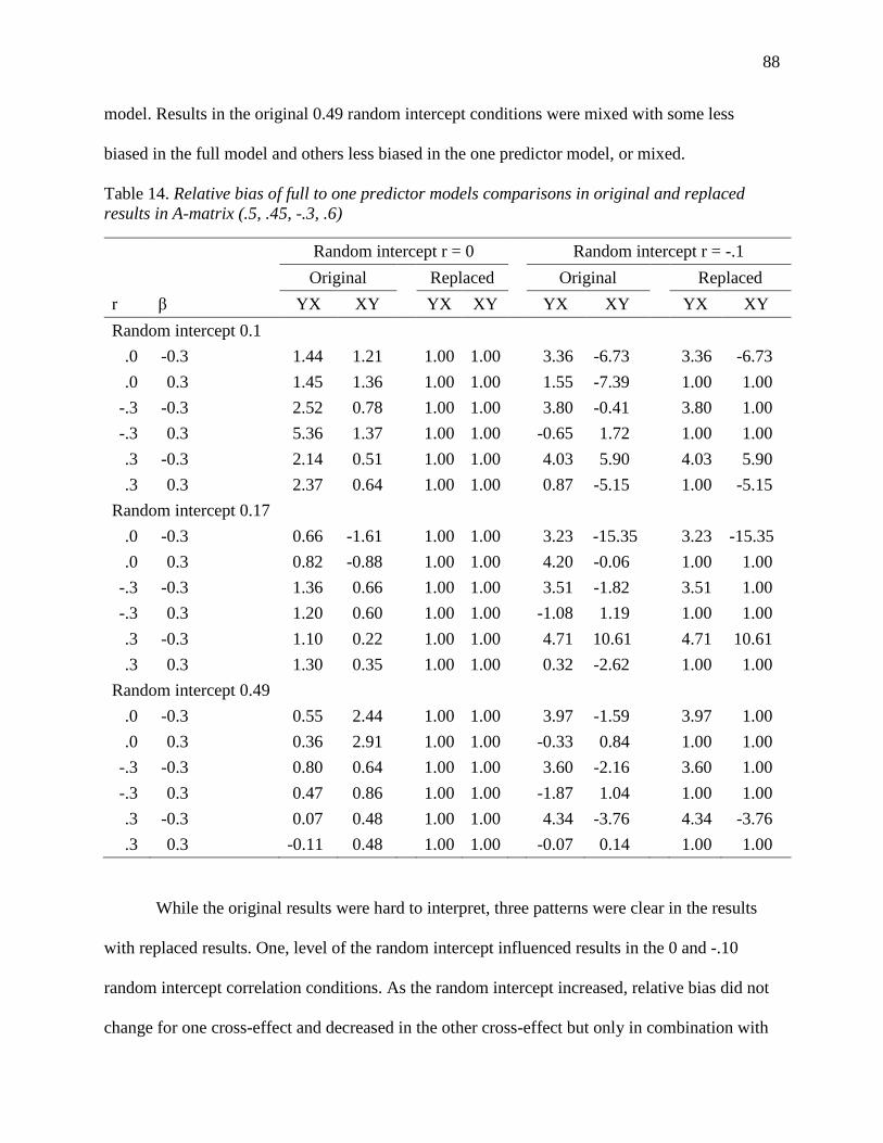
88

model. Results in the original 0.49 random intercept conditions were mixed with some less

biased in the full model and others less biased in the one predictor model, or mixed.

Table 14. Relative bias of full to one predictor models comparisons in original and replaced results in A-matrix (.5, .45, -.3, .6)

Random intercept r = 0 Random intercept r = -.1 Original Replaced Original Replaced r β YX XY YX XY YX XY YX XY Random intercept 0.1

.0 -0.3 1.44 1.21 1.00 1.00 3.36 -6.73 3.36 -6.73

.0 0.3 1.45 1.36 1.00 1.00 1.55 -7.39 1.00 1.00 -.3 -0.3 2.52 0.78 1.00 1.00 3.80 -0.41 3.80 1.00 -.3 0.3 5.36 1.37 1.00 1.00 -0.65 1.72 1.00 1.00 .3 -0.3 2.14 0.51 1.00 1.00 4.03 5.90 4.03 5.90 .3 0.3 2.37 0.64 1.00 1.00 0.87 -5.15 1.00 -5.15

Random intercept 0.17

.0 -0.3 0.66 -1.61 1.00 1.00 3.23 -15.35 3.23 -15.35

.0 0.3 0.82 -0.88 1.00 1.00 4.20 -0.06 1.00 1.00 -.3 -0.3 1.36 0.66 1.00 1.00 3.51 -1.82 3.51 1.00 -.3 0.3 1.20 0.60 1.00 1.00 -1.08 1.19 1.00 1.00 .3 -0.3 1.10 0.22 1.00 1.00 4.71 10.61 4.71 10.61 .3 0.3 1.30 0.35 1.00 1.00 0.32 -2.62 1.00 1.00

Random intercept 0.49

.0 -0.3 0.55 2.44 1.00 1.00 3.97 -1.59 3.97 1.00

.0 0.3 0.36 2.91 1.00 1.00 -0.33 0.84 1.00 1.00 -.3 -0.3 0.80 0.64 1.00 1.00 3.60 -2.16 3.60 1.00 -.3 0.3 0.47 0.86 1.00 1.00 -1.87 1.04 1.00 1.00 .3 -0.3 0.07 0.48 1.00 1.00 4.34 -3.76 4.34 -3.76 .3 0.3 -0.11 0.48 1.00 1.00 -0.07 0.14 1.00 1.00

While the original results were hard to interpret, three patterns were clear in the results

with replaced results. One, level of the random intercept influenced results in the 0 and -.10

random intercept correlation conditions. As the random intercept increased, relative bias did not

change for one cross-effect and decreased in the other cross-effect but only in combination with

89

other simulation conditions if the random intercept correlation was .10. Two, relative bias in the

.10 correlation conditions produced very cases in which both cross-effects were equally biased

but one cross-effect was equally biased 79% of the time in the full to one predictor comparison

and 81% of the time in the full to dynamic model comparison. Three, cross-effects were most

often equally biased in conditions with ±0.30 time-varying effect, 0 random intercept

correlation, and large auto-regressive terms, or 0.30 time-varying effect, -.10 random intercept

correlation, and large auto-regressive terms.

Relative efficiency. Aside from conditions with -0.05 time-varying effects, relative

efficiency results were easier to interpret than relative bias results. In the 0 random intercept

correlation conditions with ±0.30 time-varying effects, both models were more efficient in the

full model. A-matrix (.5, .45, -.3, .3) was the exception. All YX cross-effects were all less

efficiency in the full model, but XY cross-effect results varied as shown in Table 15. Relative

bias in the full to one predictor comparison depended on the level of the time-varying effect and

the time-invariant correlation, but differences were minor in most cases. Size of the random

intercept (ξ) affected results in the full to dynamic model comparison. If the random intercept

was small, relative efficiency ranged from 2.03 to 3.02 across those six conditions.

In both 0 and −.10 random intercept correlation conditions, if the time-varying effect was

−0.05, then the full and one predictor estimates were equally efficient in most cases. Only one of

the two estimates were equally efficient in the full to dynamic model comparison. For the other

time-varying effects in the −.10 random intercept correlation conditions, both estimates were

more efficient in the omitted variable models or one was more efficient in the omitted variable

models and the other was equally efficient or more efficient in the full model. Lastly, at least one

estimate was more efficient in the omitted variable models in conditions where the random

90

intercept correlation was .10. If the time-varying effect was 0.30, in many cases the other cross-

effect was also more efficient in the omitted variable models.

Table 15. Relative efficiency of XY cross-effects in A-matrix (.5, .45, -.3, .3) for 0 random intercept correlation

Time-varying β = -0.3 Time-varying β = 0.3

ξ

Time-invariant

r Full /

One predictor Full /

Dynamic

Full / One predictor

Full / Dynamic

0.10 .0 0.85 2.22 1.05 2.21 0.17 .0 0.91 0.85 0.97 0.96 0.49 .0 0.89 0.86 0.94 1.02 0.10 -.3 1.10 2.15 1.19 2.93 0.17 -.3 1.05 1.01 1.11 0.98 0.49 -.3 1.04 1.08 1.02 1.13 0.10 .3 1.00 2.03 1.26 3.02 0.17 .3 1.10 1.00 1.15 1.10 0.49 .3 1.03 1.06 1.11 1.19

One-way

Relative bias. One-way A-matrices with negative cross-lag conditions were less biased in

full model than in the omitted variable models for the 0 random intercept correlation conditions.

The exception was −0.05 time-varying effects in the comparison of the full to the one predictor

model, in which case the estimates were equally biased. In the −.10 random intercept correlation

conditions, A-matrix (.5, 0, -.3, .3) was also less biased if the time-varying effect was −0.30 or

−0.05. The only remaining conditions in which estimates for this A-matrix were less biased in

the full model was in .10 random intercept correlation and −0.30 for the time-varying effect and

the time-invariant correlation. All other conditions were pairs of more and less biased estimates

or both estimates less biased in the omitted variable models. A-matrix (.5, 0, -.3, .6) estimates

were pairs of more and less biased estimates in the −.10 random intercept correlation conditions.

91

In .10 random intercept correlation conditions, conditions with −0.30 time-varying effects and 0

or −0.30 time-invariant correlations were less biased in the full model. The remaining estimates

were both less biased in the omitted variable models or one cross-effect was less biased in the

full model and the other was less biased in the omitted variable model.

Level of random intercept affected estimates in A-matrix (.45, 0, .3, .3) in the 0 random

intercept correlation conditions. YX estimates for −0.05 and 0.30 time-varying effects were

plotted in Figure 17. In the estimates for −0.05 time-varying effect conditions, level of the

random intercept had no influence in the one predictor model but the dynamic model estimates

decreased as the random intercept increased. For the 0.30, and −0.30, time-varying effect

conditions, YX estimates decreased as random intercept increased. With respect to the pairs of

cross-effect estimates, small 0.10 random intercept conditions produced estimates that were less

biased in the one predictor model, pairs of more and less biased cross-effects if the random

intercept was 0.17, and equally biased cross-effects paired with estimates less biased in the full

model if the random intercept was 0.49. If the time-varying effect was −0.05 and the random

intercept correlation −.10, estimates were less biased in the full model. The remaining estimates

were both less biased in the omitted variable models, or one was less biased and the other was

more biased, a result more common in the full to dynamic model comparisons.

In the last A-matrix, (.5, 0, .3, .6), with ±0.30 time-varying effect conditions, one or both

cross-effects were less biased in the omitted variable models. If the time-varying effect was

−0.05 and the random intercept correlation was 0 or −.10, one estimate was always less biased in

the full model. The other estimate was equally biased or less biased in the omitted variable

models. Only in the .10 random intercept correlation conditions were both cross-effects less

biased in the omitted variable models.

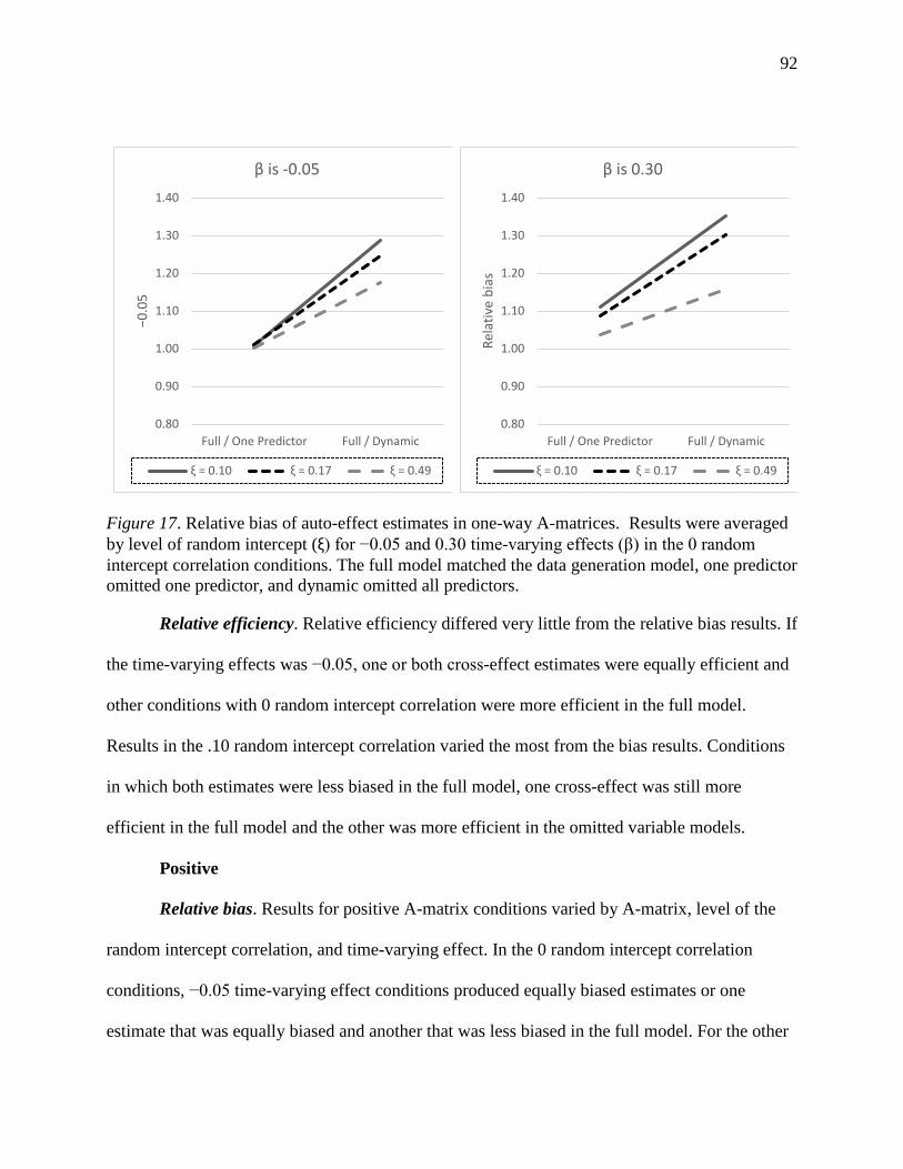
92

Figure 17. Relative bias of auto-effect estimates in one-way A-matrices. Results were averaged by level of random intercept (ξ) for −0.05 and 0.30 time-varying effects (β) in the 0 random intercept correlation conditions. The full model matched the data generation model, one predictor omitted one predictor, and dynamic omitted all predictors.

Relative efficiency. Relative efficiency differed very little from the relative bias results. If

the time-varying effects was −0.05, one or both cross-effect estimates were equally efficient and

other conditions with 0 random intercept correlation were more efficient in the full model.

Results in the .10 random intercept correlation varied the most from the bias results. Conditions

in which both estimates were less biased in the full model, one cross-effect was still more

efficient in the full model and the other was more efficient in the omitted variable models.

Positive

Relative bias. Results for positive A-matrix conditions varied by A-matrix, level of the

random intercept correlation, and time-varying effect. In the 0 random intercept correlation

conditions, −0.05 time-varying effect conditions produced equally biased estimates or one

estimate that was equally biased and another that was less biased in the full model. For the other

0.80

0.90

1.00

1.10

1.20

1.30

1.40

Full / One Predictor Full / Dynamic

−0.0

5

β is -0.05

ξ = 0.10 ξ = 0.17 ξ = 0.49

0.80

0.90

1.00

1.10

1.20

1.30

1.40

Full / One Predictor Full / Dynamic

Rela

tive

bias

β is 0.30

ξ = 0.10 ξ = 0.17 ξ = 0.49

93

levels of time-varying effects, both cross-effects were less biased in the full model. If the random

intercept correlation was −.10, −0.05 time-varying effect conditions were still equally biased

only in the 0.49 random intercept conditions in A-matrix (.5, .45, .3, .3); the other conditions

were less biased in the omitted variable models. Averages over time-varying effects for 0 and

−.10 random intercept correlations were plotted in Figure 18.

Figure 18. Relative bias of auto-effect estimates in one-way A-matrices. Results were averaged by level of random intercept (ξ) for −0.05 and 0.30 time-varying effects (β) in the 0 random intercept correlation conditions. The full model matched the data generation model, one predictor omitted one predictor, and dynamic omitted all predictors.

In A-matrix (.5, .45, .3, .3), .10 random intercept correlation conditions produced pairs of

equally biased estimate with an estimate that was less biased in one of the models, or pairs of

more and less biased estimates. A-matrix (.5, .45, .3, .6) estimates were both less biased in the

omitted variable models for ±0.30 time-varying effects; both A-matrices were less biased in the

full model if the time-varying effect was −0.05. The one exception to these patterns in the .10

random intercept correlation conditions was for conditions with .30 time-invariant correlation

0.70

0.80

0.90

1.00

1.10

1.20

1.30

1.40

1.50

1.60

Full / One Predictor Full / Dynamic

Rela

tive

bias

Random intercept r = 0

β = -0.05 β = -0.30 β = 0.30

0.70

0.80

0.90

1.00

1.10

1.20

1.30

1.40

1.50

1.60

Full / One Predictor Full / Dynamic

Rela

tive

bias

Random intercept r = -.10

β = -0.05 β = -0.30 β = 0.30

94

and −0.30 time-varying effect. Estimates were equally biased or both were less biased in the full

model.

Relative efficiency. Relative efficiency followed the same patterns as those for relative

bias in the positive A-matrices.

Negative

Relative bias. Negative A-matrix (.5, -.45, -.3, .6) produced estimates in the 0 random

intercept correlation conditions that followed a different pattern in the one predictor model than

observed in the other negative A-matrices. If the random intercept was 0.10 or 0.17 and the time-

invariant correlation was −.30, one cross-effect was less biased in the one predictor model and

the other cross-effect was less biased in the full model. If the time-invariant correlation was 0 or

.30, one estimate was equally biased and the other estimate was less biased in the full model. In

the other negative A-matrices, both estimates were less biased in the full model unless the time-

varying effect was −0.05, in which case the one predictor estimates were equally biased.

Results were very similar in the −.10 random intercept correlation conditions. Aside from

A-matrix (.5, -.45, -.3, .6), estimates were less biased in the full model if the time-varying effect

was ±0.30. A-matrix (.5, -.45, -.3, .6) was also equally biased in the −0.30 time-varying effect

conditions if the time-invariant correlation was 0 or .30; if the time-varying effect was 0.30,

results were similar to those described for the 0 random intercept correlation conditions for this

A-matrix. All estimates in the full to one predictor comparison were equally biased if the time-

varying effect was −0.05, as were the full to dynamic model comparisons as long was the time-

invariant correlation was 0 or .30. The remaining full to dynamic model comparisons were less

biased in the full model.

95

In the .10 random intercept correlation conditions, results were similar in the −0.30 time-

varying effect conditions as those for the other levels of the random intercept correlation. Results

varied by A-matrix for the −0.05 and 0.30 time-varying effects. A-matrix (.5, -.45, -.3, .3) was

equally biased. A-matrix (.5, -.45, -.3, .6) had one cross-effect that was less biased in the full

model and another cross-effect that was less biased in the omitted variable model. A-matrix (.5,

−.25, -.3, .6) produced estimates that were less biased in the omitted variable models. If the time-

varying effect was −0.05 in A-matrix (.5, -.25, -.3, .3), both estimates were less biased in the

omitted variable model, but results with 0.30 time-varying effects depended on level of the time-

invariant correlation. If the correlation was 0, one cross-effect was equally biased and the other

was less biased in the full model. If the correlation was ±.30, estimates were pairs of more and

less biased estimates or one estimate was equally biased.

Relative efficiency. Relative efficiency in negative A-matrices were the same as

described in the relative bias results except for A-matrix (.5, -.45, -.3, .3) when the random

intercept correlation was 0. In those conditions, this A-matrix produced estimates that were more

efficient in the full model, like the other negative A-matrices with ±0.30 time-varying effects.

In conditions with −0.05 time-varying effect, many of the estimates were equally efficient

in the full to one predictor comparison if the random intercept correlation was 0 or −.10. Most of

the results from the full to dynamic model comparison for the −.10 random intercept correlation

were also equally efficient. The remaining conditions produced results like relative bias results

for the near zero time-varying effect.

Time-invariant estimates

Comparisons were made between the time-invariant estimates in the full model versus the

one predictor model. Overall, simulation conditions with −.10 produced the most stable estimates

96

across all A-matrix types. The time-invariant correlation with the time-varying effect influenced

the time-invariant estimate on the random intercept. Type of A-matrix also mattered in these

results with more complex patterns observed in balanced and one-way A-matrices. Appendix

Tables B16 and B21 contain A-matrix averages of relative bias and relative efficiency

respectively.

Outliers. As shown in appendix Table B16, on average relative bias was the same with

and without outliers except for estimates in negative A-matrices. Relative efficiency did change

in both negative and balanced A-matrices. In balanced A-matrices, one time-invariant effect was

larger on average in the results with outliers but the other time-invariant effect was unaffected.

Relative efficiency changed in both time-invariant effects in negative A-matrices, as shown in

appendix Table B21. Inspection of individual conditions revealed that there were very large or

very small relative bias and efficiency results in the 0 random intercept correlation conditions.

Balanced

Relative bias. Level of random intercept correlation determined the biggest difference in

relative bias results. All conditions for random intercept correlation of −.10 were equally biased

except for A-matrix (.5, .45, -.3, .3) if the time-varying effect was −0.30 and the time-invariant

correlation was −.30 or .30. For random intercept correlation of 0.10, conditions with a time-

invariant correlation of 0.30 produced relative bias results that were equally biased in one

estimate and less biased in the omitted variable model for the other. The remaining estimates for

.10 random intercept correlation conditions were equally biased. For random intercept

correlations of 0, relative bias differed by level of the random intercept, level of time-varying

effect, or some combination of those conditions.

97

In the case of zero random intercept correlation, if the time-invariant correlation was also

zero, estimates were equally biased across all levels of the time-varying effect. If the time-

invariant correlation and the effect were opposite in sign, (−.30, 0.30) or (−0.30, 0.30), the

effects on trait variance were less biased in the full model. In the conditions where the time-

varying effect was −0.05 and time-invariant correlation was −.30, one estimate was equally

biased and the other was less biased in the full model. For that same −0.05 time-varying effect, if

the time-invariant correlation was .30, then one effect was equally biased and the other was less

biased in the full model. Lastly, if the time-invariant correlation and effect were both −0.30 or

0.30, then the one predictor model was less biased. Results for both relative bias and efficiency

are shown in Table 16.

Table 16. Relative bias and efficiency for estimates of time-invariant effects on trait variance in balanced A-matrices, –YX, and 0 random intercept correlation averaged across conditions

Relative bias Relative efficiency r β TI on X TI on Y TI on X TI on Y r = 0 0.00 −0.05 1.00 1.00 1.01 1.00 0.00 −0.30 0.99 0.98 0.95 0.95 0.00 0.30 0.99 0.98 0.95 0.95

Opposite sign −0.30 0.30 0.54 0.82 0.31 0.68 0.30 −0.05 0.87 0.97 0.77 0.93 0.30 −0.30 0.54 0.82 0.31 0.68

Same sign −0.30 −0.05 1.19 1.04 1.32 1.07 −0.30 −0.30 5.82 1.74 2.12 2.08 0.30 0.30 6.57 1.21 5.54 1.46

98

Relative efficiency. Relative efficiency results differed very little from the relative bias

results described above. Most importantly, in almost all cases results that were equally biased

were also equally efficient.

One-way

Relative bias. Results for zero random intercept correlation simulation conditions varied

by levels of time-varying effect, time-invariant correlation, or both. If the time-invariant

correlation was 0, the models were equally biased. A −.30 time-invariant correlation with −0.30

time-varying effect produced estimates that were less biased in the one predictor model; if the

time-varying effect was −0.05 one of the two estimates was still less biased in the one predictor

model but one was equally biased, and both were less biased in the full model if the time-varying

effect was 0.30. Like the negative pair of conditions, 0.30 for both time-invariant correlation and

time-varying effect resulted in estimates that were less biased in the full model. If those

conditions were opposite in sign, one negative and one positive, both estimates were less biased

in the full model. The remaining −0.05 time-varying effect conditions were equally biased.

Estimates were equally biased in the −.10 random intercept correlation conditions except

in A-matrix (.5, 0, .3, .3). In those conditions, estimates were less biased in one predictor model

if the time-invariant and time-varying effect were 0.30; the other conditions were less biased in

the full model. If the random intercept correlation was .10, models with time-varying effects

−0.30 and −0.05 were equally biased. Estimates were also equally biased if the time-invariant

correlation and time-varying effect were −.30 and 0.30 respectively. In the other 0.30 time-

varying effect conditions, one or both estimates were less biased in the one predictor model.

Relative efficiency. Relative efficiency results for time-invariant estimates in the one-

way A-matrices followed the same patterns described above for relative bias. If the results

99

differed, the relative efficiency values became smaller if less than 1 or larger if relative bias was

greater than 1. In a few cases where one time-invariant estimate was equally biased but slightly

above 1, relative efficiency could be greater than 1.10 so both estimates were now more efficient

in the omitted variable model.

Positive

Relative bias. Time-invariant correlation, time-varying effect, and random intercept

correlation all played a role in relative bias in positive A-matrices. Most −0.05 time-varying

effect conditions were equally biased. Within 0 random intercept correlation conditions, if both

time-invariant correlation and time-varying effects were −0.30 or 0.30, one estimate was equally

biased and the other was less biased in one predictor model. If the effect and correlation were

opposite in sign (.30 and −0.30 or −.30 and 0.30), one estimate was equally biased and the other

was less biased in the full model. The other conditions were equally biased. If the random

intercept correlation was −.10, A-matrix (.5, .45, .3, .6) results were equally biased except if the

time-varying effect was −0.30 and the time-invariant correlation was 0 or −.30, in which case

results were less biased in the one predictor model. A-matrix (.5, .45, .3, .3) full model estimates

were equally biased or less biased in one effect on trait variance and less biased in the other

effect. In the .10 random intercept correlation conditions with -.3 or .3 for both time-invariant

correlation and time-vary effects, estimates were equally biased in one estimate and less biased

in the one predictor model or both estimates were less biased in the one predictor model. The

effect on X trait variance was less biased in the full model in the remaining 0.30 time-varying

effect conditions. The effect on Y trait variance was also less biased in the full model in A-

matrix (.5, .45, .3, .3) and less biased in the one predictor model in A-matrix (.5, .45, .3, .6). Bias

100

averages by combination of time-invariant correlation and time-varying effect are listed in Table

17.

Table 17. Relative bias and efficiency for A-matrix (.5, .45, .3, .3) with 0 random intercept correlation

(.5, .45, .3, .3) (.5, .45, .3, .6) r β TI on X TI on Y TI on X TI on Y 0.00 −0.05 0.98 1.02 1.01 1.01 0.00 −0.30 1.02 1.01 1.07 1.06 0.00 0.30 0.94 1.11 0.84 0.89

−0.30 −0.05 1.06 0.99 1.00 0.99 −0.30 −0.30 1.24 1.01 1.19 1.14 −0.30 0.30 0.84 1.06 0.82 0.89 0.30 −0.05 0.96 1.05 1.03 1.05 0.30 −0.30 1.00 0.99 0.99 0.99 0.30 0.30 0.94 1.22 1.21 1.15

Relative efficiency. Relative efficiency results were similar to relative bias results. The

main difference was in relative bias less than 0.95 or greater than 1.05. If relative bias was

outside of that range, relative efficiency was even further away from one in the same direction.

For example, if relative bias was 0.94, then relative efficiency might be 0.89 more efficient in the

full model. Estimates between 0.95 and 1.05 remained equally efficient.

Negative

Relative bias. The level of the random intercept condition affected whether the estimates

were equally biased or not. All conditions with −.10 random intercept correlation were equally

biased as were most conditions with 0.10 random intercept correlation. In the positive correlation

conditions, the conditions that were not equally biased were less biased in the one predictor

model. Along with a small or medium random intercept, all conditions had a time-invariant

correlation of .3 with time-varying effect −0.05, 0 time-invariant correlation with 0.30 time-

101

varying effect, or correlation and effect that were both 0.30. Relative bias ranged from 1.09 to

1.28 for the effect on X trait variance, and from 1.08 to 1.26 for the effect on Y trait variance. In

conditions with 0 random intercept correlations, results depended on the combination of time-

invariant correlation and the time-varying effect, if they were both .3 or −.30, then the results

were more efficient in the one predictor model. They were also more efficient in the one

predictor model if the time-invariant correlation was −.30 and the time-varying effect was −0.05.

Equally biased conditions were few with most in the 0 time-invariant correlation paired with

−0.05 time-varying effect. The remaining conditions were less biased in the full model. Averages

by combination of time-invariant correlation and time-varying effect are listed in Table 18.

Table 18. Relative bias and efficiency for estimates of time-invariant effects on trait variance in negative A-matrices with 0 random intercept correlation averaged across conditions

Relative bias Relative efficiency TI r β TI on X TI on Y TI on X TI on Y 0.00 −0.05 0.96 0.96 0.94 0.94 0.00 −0.30 0.83 0.84 0.68 0.72 0.00 0.30 0.83 0.84 0.67 0.72

−0.30 −0.05 1.12 1.08 1.20 1.14 −0.30 −0.30 3.31 1.74 2.12 2.08 −0.30 0.30 0.46 0.52 0.24 0.31 0.30 −0.05 0.84 0.86 0.75 0.79 0.30 −0.30 0.46 0.52 0.25 0.31 0.30 0.30 -8.33 1.74 2.09 2.06

Relative efficiency. Relative efficiency results were identical to the relative bias results.

Averages for the .10 random intercept correlations that were more efficient in the one predictor

model ranged from 1.10 to 1.67 for the effect on X trait variance. For Y trait variance on those

same conditions, relative efficiency ranged from 1.08 to 1.65. Average relative efficiency for the

0 random intercept correlation conditions are shown in Table 18.

102

Discussion

Type of A-matrix followed by level of random intercept correlation influenced relative

bias and relative efficiency the most in simulation 2, the evaluation of how to omitting time-

varying predictor changes, or not, model estimates. Of particular interest was that no A-matrix

was robust to the omitted time-varying predictor for all three types of estimates examined, auto-

effects, cross-effects, and time-invariant effects, in all simulations conditions. At best, a model

might be robust in all of the three estimate types if the random intercept correlation was not zero.

With the focus was on larger patterns given the 1296 simulation conditions that were part of this

study, outliers did not drastically affect results because dropping outliers just reduced the range

for results on a simulation condition. Therefore, the discussion will focus on the results with

outliers removed.

Some estimates were biased in the full model with results in the omitted variable models

biased as well. Bias was relatively equal in some cases with differences identified in efficiency.

In other cases, the omitted variable model produced estimates that were less biased and more

efficient than the full model. If only cases in which estimates were equally biased and efficient

were considered robust, only one negative A-matrix produced robust auto- and cross-effects in a

subset of conditions. Aside from small time-varying effect conditions, there were a few other

conditions spread across the other A-matrix types that drift parameters that were robust to the

omitted variable variance. Time-invariant effects were the most robust across the simulations

conditions but only half of those estimates were equally biased and efficient. All of the results

discussed below included conditions in which estimates were equally biased and equally

efficient, conditions in which both were less biased and more efficient in the omitted variable

models, or conditions in which it was a combination of those. Under the conditions of this

103

simulation, including all of those results as robust provided better guidance than just including

only equally biased and efficient results.

Aside from the small time-varying effect conditions and positive A-matrix conditions,

there were few cases in which auto-effect estimates were equally biased, equally efficient, or

both. Balanced A-matrices estimates were only robust if the time-varying effect was near zero,

and then not in every condition. In negative A-matrices, the only exception was for −0.05 time-

varying effect conditions, conditions in which one would expect to find estimates robust to

omission due to the size of the effect, and in a group of conditions in which the time-varying

effect and correlation with the random intercept were both positive. One-way A-matrices were

robust to the omitted variable in the full to one predictor condition for the smallest time-varying

effect if the time-varying effect and random intercept were not related. If they were related, some

of the other auto-effects were less biased in both omitted variable models. Positive A-matrices

produced robust auto-effects in approximately half of its conditions. The size of the auto-

regressive, level of correlation between the time-varying effect and the random intercept, and

time-varying effects all influenced the most.

These auto-effect results were worse than expected, in particular for the small time-

varying effect condition, a condition in which the omission was not expected to impact any

results. The other interesting part of these results were the fact that negative and positive A-

matrices were robust in this condition, two A-matrix types that would be considered unstable. It

is possible that the variance from the omitted variable helped to stabilize the estimates to a small

degree.

More promising were the cross-effect estimates. In the positive A-matrices and in many

conditions in the one-way A-matrices, the models were robust to the omitted variable. The

104

results for the one-way A-matrices did vary by level of the random intercept correlation and

whether the nonzero cross-lag condition was positive or negative. Only positive cross-lag

conditions were robust to the omitted variable variance. And for the A-matrices with a small

auto-regressive condition, only −.10 and .10 random intercept correlations were robust to the

omission. Those same correlation conditions affected cross-effect estimates for positive A-

matrices, producing robust estimates. Most cross-effects in negative A-matrices were impacted

by the omitted variable variance. There was only one negative A-matrix that returned different

results in 9 conditions, all with positive time-varying effects and positive random intercept

correlation.

Balanced A-matrix results were unclear due to the small size of bias in the model

estimates with even smaller differences in many cases. Treating estimates that were minimally

different as equally biased clarified the results. Most conditions returned at least one cross-effect

that was equally biased. If the random intercept was small, it was likely that the other estimate

was equally biased or less biased in the omitted variable models. The decision to evaluate

balanced A-matrices in this manner was an attempt to understand the relative bias results.

Relative efficiency results for the balanced cross-effects, results that were not processed again,

indicated that small and medium intercepts conditions were the most robust if the random

intercept correlation was not zero. If the random intercept correlation was zero, only one

predictor model estimates were equally biased and efficient in small time-varying effect

conditions. Based on all of the results, cross-effects were relatively equal across models.

With respect to time-invariant predictors, if there was no correlation between the random

intercept and the time-varying effect, combinations of time-varying effect and the correlation

between the time-varying effect and the time-invariant effect determined whether estimates were

105

equally biased and efficient. If they were both strong but different signs (e.g. -0.30 and .30),

those conditions were less biased in the full model as were those conditions with 0 time-invariant

correlation. Otherwise, time-invariant estimates were robust in the remaining 0 random intercept

correlation conditions. For all A-matrices, most conditions with −.10 and .10 random intercept

correlations were robust to the omitted variable variance.

Looking at the bigger picture, variance from the omitted variable influenced estimates the

time-varying estimates in the positive A-matrix conditions, conditions that were most robust in

the estimation of the dynamic process. For the other combinations of cross-effects, whether a

correlation existed between the time-varying predictor and other parameters influenced results

the most. If there was a covariance of −.10 or .10 between time-varying effect and random

intercept, more estimates overall were robust to the omitted variable.

Aside from type of A-matrix, the simulation condition for correlation between the time-

varying effect and the random intercept influenced results the most. If no correlation existed,

very few auto- and cross-effects were robust to the omitted variable. The existence of that

parameter may have provided an alternate path for the variance in the model so that the variance

did not affect the dynamics to the degree it did when the correlation was zero. All models

enabled the estimation same parameters but zero correlation conditions were not able to recover

the estimate as well.

106

Chapter 5: Conclusion

In order to reflect the complexity of real data drift parameters, time-invariant correlations,

trait variance, predictor effects, and trait variance/predictor correlations were all varied in this

study. No estimates were robust to omission of a variable across all conditions, in either

simulation. There were cases in which estimates were equally biased and efficient, and cases that

depended on two or more simulation conditions. Within some conditions, the omitted variable

model estimates were less biased and more efficient. The largest pattern observed in both

simulations was pairs of results in which one estimate (e.g., X auto-effect) was less biased or

more efficient in the full model and another estimate (e.g., Y auto-effect) was less biased or more

efficient in the omitted variable model.

In simulation 1, some drift parameters (auto-effects and cross-effects) were expected to

be robust to the omitted variable variance regardless of the A-matrix simulation conditions.

When the effect of the time-invariant variable was near zero, drift estimates were robust to

omission of the time-invariant variable in 30% of the conditions. For the other conditions, 65%

estimates were either equally biased or equally efficient but not both. If bias differences less than

0.01 are considered equally biased, then the more than 90% of the estimates were equally biased.

If the time-invariant effects were ±0.30 and both cross-effects were positive, the size of trait

variance influenced estimates such that 2/3 but not all conditions were robust. Once both time-

invariant predictors were omitted from the model, the only simulation conditions that produced

equally biased and efficient estimates, or estimates in which estimates were less biased and more

efficient in the omitted variable model, were conditions with two positive cross-effects. Drift

estimates were not affected by the presence or absence of a correlation between the time-

invariant predictors in the model, but the time-invariant effects were.

107

For the time invariant predictor in simulation 1, the effect of the predictor was biased in

the model that included both time-invariant predictors and the model with a single time-invariant

predictor. Whether the estimate was robust to the omitted variable depended on how the two

time-invariant predictors were related to each other. Estimates were most robust if the two

predictors were orthogonal, if the correlation between the time-invariant predictor and omitted

variable effect were both positive, or if the correlation between the time-invariant predictor and

omitted variable effect were both negative. For the time-variant predictor correlation and time-

invariant effect simulation conditions, if one condition was negative and the other condition was

positive, the estimates were not robust to being omitted from the model. Equal strength but

opposite signed appeared to produced estimates that were less biased and more efficient only

when both time-invariant predictors are included in the model.

In simulation 2, the relationship between the time-invariant and time-varying predictors

was expected to bias estimates when these predictors were not modeled. The correlation between

the time-varying and time-invariant predictors affected time-invariant estimates, but not drift

estimates. Aside from conditions where the time-varying predictor effect was near zero, in which

cases conditions were generally robust, drift parameters were most often robust if the omitted

variable was correlated with trait variance and the auto-effect was strong. Whether the omitted

variable effect was positive or negative mattered only in the case of two negative cross-effects,

where a positive effect produced estimates less biased and more efficient in the omitted variable

models. If the time-varying predictor was orthogonal to trait variance, drift results were similar

to those in simulation 1, as were results for time-invariant effects. If the trait variance was

correlated with the omitted variable, most time-invariant estimates were robust to the omitted

variable variance.

108

In both simulations, estimates were not always equally biased and efficient if the omitted

variable effect was near zero, but in many cases the estimate was equally biased or equally

efficient. If the omitted variable effect was strong, then omitting the variable did matter to one or

more estimates in the model, supporting work by Mauro (1990). If the two predictors were

correlated, time-invariant effects were expected to be biased, however results also depended on

the level of the omitted variable’s effect. As anticipated, how omitted variables influence other

predictors is more complex than identified with single level regression (Cohen et al., 2003;

Singer & Willett, 2003).

Some estimates were robust in both simulations, but they were expected to be biased.

When cross-effects are both positive or both negative, the dynamic process can be expected to be

less stable, as cross-effects in the same direction can lead to a feedback loop. Given this

instability, results were expected to be similar when the cross-effects were both positive or

negative. Data generated with two negative cross-effects did not return estimates that were robust

to omitted variables except in a few specific conditions. On the other hand, estimates from

simulation conditions with two positive cross-effects improved the most once the predictor was

omitted from the model. Conditions with two positive cross-effects, on the other hand, were

robust to the omission. As for why the A-matrices with positive cross-effects benefitted from the

omitted variable, the variance from the omitted variable could have acted as additional input that

added stability to the system (Åström & Murray, 2008). If all the unstable systems needed was

extra variance to obtain robust estimates, however, then both the dual-negative and dual-positive

sets of simulation conditions should have returned robust estimates. However, only conditions

with two positive cross-effects consistently returned robust estimates.

109

Underlying all of these relative bias and efficiency results were estimates that were

biased, but no more than expected in many cases. Based on previous simulations (Oud, 2007),

bias was expected to be approximately 10% of the size of the estimate. Estimate bias was larger

than anticipated in two A-matrices with small auto-regressive and large cross-lag conditions. In

these two A-matrices, the amount of bias in auto- and cross-effects ranged from 14 to 36% of the

true value. The cause of the extra bias was unclear, nor was it clear if the extra bias influenced

relative bias and relative efficiency results.

Limitations and future directions

Results from this study were more complex than anticipated, starting with some warning

messages in the data generation process and some unrealistic auto-effect estimates. Even after

the removal of outliers to better observe patterns in the results, estimates were robust only in

combinations of conditions, but never across all conditions within a simulation. Lack of simpler

results may be due to the selection of simulation conditions. The broad range of conditions meant

that the simulations provided some information about robust estimates. Whether those results can

be reproduced over a range of values within will require additional study. The drift matrix

conditions should be extended to include stronger auto-effects and weaker cross-effects.

Although each A-matrix identified for the simulation conditions met the mathematical condition

for stability (Hamilton, 1994), some combinations selected for this study were more stable than

other combinations. After clarifying how these cross-effects relate to auto-effects in substantive

research and obtaining a better understanding of the mathematics related to dynamics, a more

appropriate set of cross-effect conditions should be selected for future studies.

The near zero condition of the omitted variable variance produced estimates that were not

always robust. Because of the other conditions in which presence or lack of a relationship

110

appeared to influence estimates, a true zero condition may produce results different from a near

zero condition. Testing the difference and the point at which the distance from 0 matters could

clarify the results for one-way A-matrices and for the time-invariant effects.

The single sample size of 200 was selected for the study based on the expectation that

omitted variable variance would influence the models like measurement error affected estimates

(Shaw, 2015), and if so then sample size would not matter. Because hypotheses based on the

measurement error assumption did not hold, the sample size should be revisited in future studies.

Oud and colleagues (Oud, 2007; Oud & Singer, 2008) indicated that sample size needed to be

700 or greater if trait variance was going to be included in the model. Although many

psychology studies use samples much smaller than 700, the role of sample size should be

explored with respect to omitted variables.

Determining whether an estimate was robust or not depended on bias, relative bias, and

relative efficiency results. Within this study, these statistics able to describe whether the

statistical differences were truly different such that the difference matters to the substantive

researcher. For example, if bias in one model was 0.005 and bias in the compared model was

0.0008, relative bias was large but the practical effect of that difference was minimal. If absolute

differences in bias are less than 0.01 in estimates, the conclusions drawn in substantive research

are not likely to change due to omitted variable variance.

If some assumptions are made about the variable left out of the model, the results from

this study can inform substantive research practices. In all cases, time-invariant predictors, time-

varying predictors, and dynamic processes will be omitted from the model. If the omitted time-

varying predictor is related to trait variance captured in the model, then estimates for the time-

invariant predictors in the model should be robust to omission. As for the drift estimates, the

111

results are less clear for two reasons. One, estimates were more biased and unequally biased

across models so more research is needed before definitively making a judgment about the

robustness of the estimates. Two, some simulation conditions returned estimates that changed so

little from one model to the next that the substantive researcher would not notice but resulted in

extremely large or very small relative bias and efficiency values. Once these two issues are

resolved, further guidance can be provided.

Regardless of where future research begins, amount of bias and efficiency needs to be

taken into account as does determining why some conditions were more biased than anticipated.

Building up a simulation from a simple omitted variable scenario to one more complex, and

reflective of real data, should more clearly determine conditions under which the EDM estimates

will be robust. Maybe EDM estimates will always depend upon a combination of conditions as

seen in this study. Or, results may become clearer with estimates that will always be robust along

with estimates that will always be biased. If the story can be simplified, that will benefit both

methods and substantive researchers, because variables will always be omitted from models in

substantive research. The models that psychologists develop are not getting simpler so

methodologists need to increase the complexity of simulations, enabling researchers to make

more informed decisions.

112

References

Åström, K.J., & Murray, R.M. (2008). Feedback systems: An introduction for scientists and

engineers. Princeton, NJ: Princeton University Press.

Beck, N., & Katz, J.N. (1996). Nuisance vs. Substance: Specifying and estimating time-series-

cross-section models. Political Analysis, 6(1), 1-36.

Box, G.E., & Jenkins, G.M. (1976). Time series analysis: Forecasting and control, revised ed.

Oakland, CA: Holden-Day.

Brockwell, P.J., & Davis, R.A. (2002). Introduction to time series and forecasting (2nd ed.).

Verlag, NY: Springer.

Carsey, T.M., & Harden, J.J. (2014). Monte carlo simulation and resampling methods for the

social sciences. Los Angeles, CA: Sage Publications, Inc.

Cohen, J., Cohen, P., West, S.G., & Aiken, L.S. (2003). Applied multiple regression/correlation

analysis for the behavioral sciences (3rd ed.). Mahwah, NJ: Lawrence Erlbaum

Associates.

Driver, C.C., Oud, J.H.L., & Voelkle, M.C. (n.d.). Continuous time structural equation model

with r package ctsem. Journal of Statistical Computing.

Efron, B., & Tibshirani, R.J. (1993). An introduction to the bootstrap. New York: Chapman &

Hall.

Goulet, V., Dutang, C., Maechler, M., Firth, D., Shapira, M., Stadelmann, M., & expm-

developers@lists.R-forge.R-project.org. (2015). Expm: Matrix exponential (Version

0.999-0) [R package]. Retrieved from http://CRAN.R-project.org/package=expm

Granville, W.A., Smith, P., & Langley, W.R. (1957). Elements of the differential and integral

calculus. Chicago: Ginn & Co.

113

Hamaker, E.L., Dolan, C.V., & Molenaar, P.C. (2002). On the nature of sem estimates of arma

parameters. Structural Equation Modeling: A Multidisciplinary Journal, 9(3), 347-368.

Hamaker, E.L., Dolan, C.V., & Molenaar, P.C. (2003). Arma-based sem when the number of

time points t exceeds the number of cases n: Raw data maximum likelihood. Structural

Equation Modeling: A Multidisciplinary Journal, 10(3), 352-379.

Hamaker, E.L., Kuiper, R.M., & Grasman, R.P. (2015). A critique of the cross-lagged panel

model. Psychological Methods, 20(1), 102.

Hamilton, J.D. (1994). Time series analysis. Princeton, New Jersey: Princeton University Press.

James, L.R. (1980). The unmeasured variables problem in path analysis. Journal of Applied

Psychology, 65(4), 415-421.

Keele, L., & Kelly, N.J. (2006). Dynamic models for dynamic theories: The ins and outs of

lagged dependent variables. Political Analysis, 14(2), 186-205.

Kennedy, P. (2008). A guide to econometrics (6th ed.). Oxford: Blackwell Publishing.

Kline, R.B. (2011). Principles and practice of structural equation modeling (3rd ed.). New York,

NY: Guilford Press.

Mauro, R. (1990). Understanding love (left out variables error): A method for estimating the

effects of omitted variables. Psychological Bulletin, 108(2), 314-329.

Muthén, L.K., & Muthén, B.O. (1998-2015). Mplus: Statistical analysis with latent variables:

User's guide. Los Angeles: Muthén & Muthén

Neale, M.C., Hunter, M.D., Pritikin, M.Z., Brick, T.R., Kickpatrick, R.M., Estabrook, R., . . .

Boker, S.M. (2016). Openmx 2.0: Extended structural equation and statistical modeling.

Psychometrika, 80(2), 535-549. doi: 10.1007/s11336-014-9435-8

114

Oud, J.H., & Jansen, R.A. (2000). Continuous time state space modeling of panel data by means

of sem. Psychometrika, 65(2), 199-215.

Oud, J.H.L. (2007). Comparison of four procedures to estimate the damped linear differential

oscillator for panel data. In K. v. Montfort, J. H. L. Oud & A. Satorra (Eds.),

Longitudinal models in the behavioral and related sciences (pp. 19-39). Mahwah, NJ:

Erlbaum.

Oud, J.H.L., & Singer, H. (2008). Continuous time state space modeling of panel data: Sem

versus filter techniques. Statistica Neerlandica, 62(1), 4-28.

R Core Team. (2017). R: A language and environment for statistical computing. Vienna, Austria:

R Foundation for Statistical Computing.

Raudenbush, S.W., & Bryk, A.S. (2002). Hierarchical linear models: Applications and data

analysis methods (Vol. 1): Sage.

Shaw, L.A. (2015). The impact of measurement error on continuous time panel models.

University of Kansas. ProQuest Dissertations & Theses Global database.

Singer, J.D., & Willett, J.B. (2003). Applied longitudinal data analysis: Modeling change and

event occurrence. New York, NY: Oxford University Press.

Stimson, J.A. (1985). Regression in space and time: A statistical essay. American Journal of

Political Science, 914-947.

Tofighi, D., West, S.G., & MacKinnon, D.P. (2013). Multilevel mediation analysis: The effects

of omitted variables in the 1–1–1 model. British Journal of Mathematical and Statistical

Psychology, 66(2), 290-307.

van Buuren, S. (1997). Fitting arma time series by structural equation models. Psychometrika,

62(2), 215-236.

115

Voelkle, M.C., & Oud, J.H. (2013). Continuous time modelling with individually varying time

intervals for oscillating and non‐oscillating processes. British Journal of Mathematical

and Statistical Psychology, 66(1), 103-126.

Voelkle, M.C., Oud, J.H., Davidov, E., & Schmidt, P. (2012). An sem approach to continuous

time modeling of panel data: Relating authoritarianism and anomia. Psychological

methods, 17(2), 176.

Voelkle, M.C., & Oud, J.H.L. (2015). Relating latent change score and continuous time models.

Structural Equation Modeling: A Multidisciplinary Journal, 22(3), 366-381. doi:

10.1080/10705511.2014.935918

A1

Appendix A: Supplementary Simulation 1 Tables

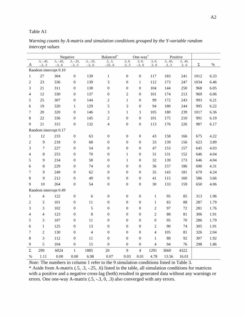
A2

Table A1

Warning counts by A-matrix and simulation conditions grouped by the Y-variable random intercept values

Negative Balanced* One-way* Positive A

.5, -.45, -.3, .3

.5, -.45, -.3, .6

.5, -.25, -.3, .3

.5, -.25, -.3, .6

.5, .3, -.25, .6

.5, 0,

.3, .3 .5, 0, -.3, .6

.5, 0,

.3, .6 .5, .45, .3, .3

.5, .45, .3, .6 Σ %

Random intercept 0.10 1 27 304 0 139 1 0 0 117 183 241 1012 6.33 2 23 336 0 139 3 0 1 112 173 247 1034 6.46 3 21 311 0 138 0 0 0 104 144 250 968 6.05 4 12 330 0 137 0 2 0 101 174 213 969 6.06 5 25 307 0 144 2 1 0 99 172 243 993 6.21 6 19 320 1 129 5 3 0 94 180 244 995 6.22 7 20 320 0 146 3 1 3 105 180 239 1017 6.36 8 22 336 0 145 2 0 0 101 175 210 991 6.19 9 21 315 0 132 4 0 0 113 176 226 987 6.17 Random intercept 0.17 1 12 233 0 63 0 0 0 43 158 166 675 4.22 2 9 218 0 68 0 0 0 33 139 156 623 3.89 3 7 227 0 54 0 0 0 47 153 157 645 4.03 4 8 253 0 70 0 1 0 31 131 152 646 4.04 5 9 234 0 58 0 1 0 32 139 173 646 4.04 6 8 229 0 74 0 0 0 36 157 186 690 4.31 7 9 249 0 62 0 0 0 35 143 181 679 4.24 8 9 212 0 49 0 0 0 41 115 160 586 3.66 9 10 264 0 54 0 0 0 30 133 159 650 4.06 Random intercept 0.49 1 4 122 0 6 0 0 0 1 95 85 313 1.96 2 3 101 0 11 0 0 0 1 83 88 287 1.79 3 3 102 0 5 0 0 0 2 97 72 281 1.76 4 4 123 0 8 0 0 0 2 88 81 306 1.91 5 3 107 0 11 0 0 0 0 95 70 286 1.79 6 1 125 0 13 0 0 0 2 90 74 305 1.91 7 2 130 0 4 0 0 0 4 105 81 326 2.04 8 3 112 0 11 0 0 0 1 88 92 307 1.92 9 5 104 0 15 0 0 0 4 94 76 298 1.86 Σ 299 6024 1 1885 20 9 4 1291 3660 4322 % 1.11 0.00 0.00 6.98 0.07 0.03 0.01 4.78 13.56 16.01 Note: The numbers in column 1 refer to the 9 simulation conditions listed in Table 3. * Aside from A-matrix (.5, .3, -.25, .6) listed in the table, all simulation conditions for matrices with a positive and a negative cross-lag (both) resulted in generated data without any warnings or errors. One one-way A-matrix (.5, -.3, 0, .3) also converged with any errors.

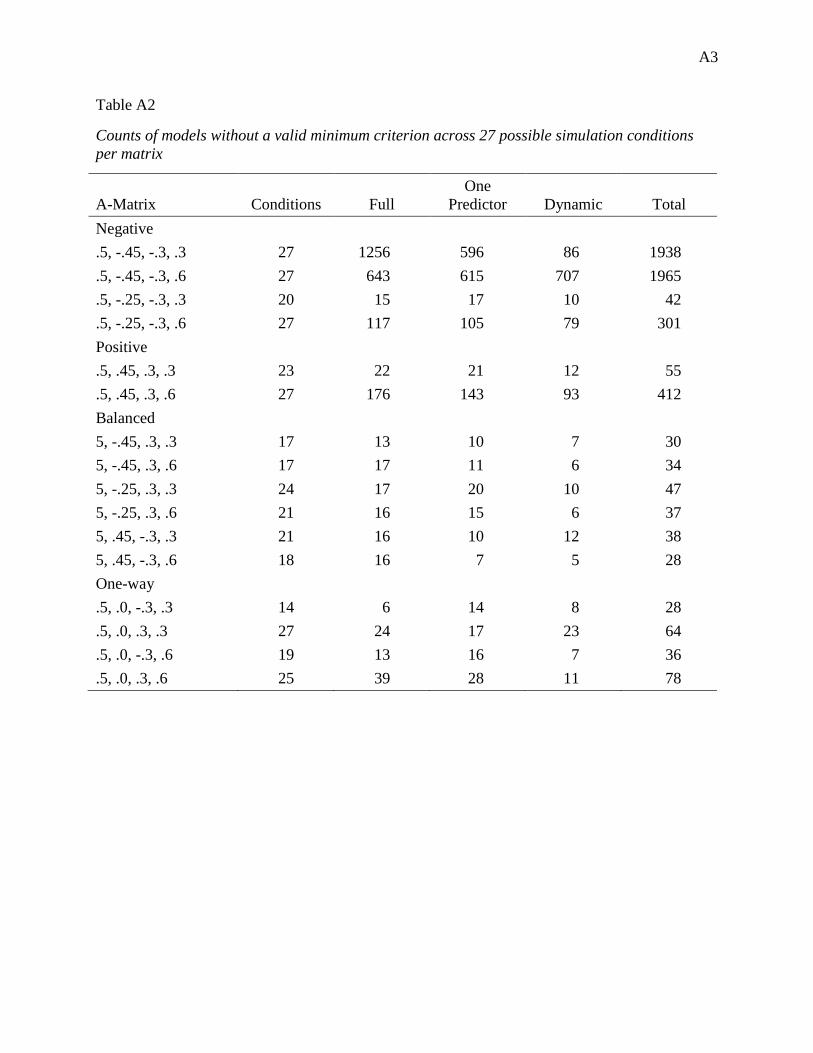
A3

Table A2

Counts of models without a valid minimum criterion across 27 possible simulation conditions per matrix

A-Matrix Conditions Full One

Predictor Dynamic Total Negative .5, -.45, -.3, .3 27 1256 596 86 1938 .5, -.45, -.3, .6 27 643 615 707 1965 .5, -.25, -.3, .3 20 15 17 10 42 .5, -.25, -.3, .6 27 117 105 79 301 Positive .5, .45, .3, .3 23 22 21 12 55 .5, .45, .3, .6 27 176 143 93 412 Balanced 5, -.45, .3, .3 17 13 10 7 30 5, -.45, .3, .6 17 17 11 6 34 5, -.25, .3, .3 24 17 20 10 47 5, -.25, .3, .6 21 16 15 6 37 5, .45, -.3, .3 21 16 10 12 38 5, .45, -.3, .6 18 16 7 5 28 One-way .5, .0, -.3, .3 14 6 14 8 28 .5, .0, .3, .3 27 24 17 23 64 .5, .0, -.3, .6 19 13 16 7 36 .5, .0, .3, .6 25 39 28 11 78

A4

Table A3

Descriptive statistics of bias across all 432 simulation conditions with all converged models

Mean SD Median Min. Max. Range Skew Kurtosis

Full

X -3.39 15.31 0.04 -102.85 0.27 103.12 -4.77 22.08 YX -3.70 16.58 0.00 -112.01 3.93 115.94 -4.78 22.23 XY -5.17 23.58 0.00 -160.82 0.26 161.08 -4.86 23.10 Y -5.54 25.60 0.04 -175.35 0.60 175.94 -4.87 23.21 Trait X on TI1 2.63 12.85 -0.20 -0.43 86.15 86.57 4.81 22.55 Trait Y on TI1 2.82 13.93 -0.23 -0.37 93.85 94.21 4.83 22.68 Trait X on TI2 -0.21 9.83 0.03 -79.02 65.06 144.08 -1.37 38.95 Trait Y on TI2 -0.23 10.66 0.03 -86.13 70.65 156.78 -1.38 39.15 One predictor

X -1.58 9.01 0.05 -87.22 0.28 87.49 -7.12 54.12 YX -1.75 9.74 0.00 -94.92 0.22 95.14 -7.14 54.51 XY -2.44 13.81 0.00 -136.51 0.27 136.78 -7.24 56.12 Y -2.57 14.99 0.05 -148.70 0.63 149.33 -7.25 56.31 Trait X on TI1 1.13 7.57 -0.22 -0.43 77.25 77.69 7.30 57.41 Trait Y on TI1 1.19 8.20 -0.28 -0.45 84.08 84.53 7.32 57.74 Dynamic

X -0.19 1.59 0.06 -15.98 0.60 16.57 -7.23 56.28 YX -0.25 1.70 0.01 -16.98 0.68 17.66 -7.20 55.74 XY -0.35 2.38 0.02 -23.67 1.12 24.79 -7.23 56.25 Y -0.30 2.59 0.07 -25.49 1.19 26.68 -7.18 55.28

A5

Table A4

Model count by level of random effect and A-matrix type after removal of model estimates with unrealistic auto-effect < -4.0 Model Percent

A-matrix Full One

predictor Dynamic Total By A-matrix Random Intercept 0.10

Negative .5, -.45, -.3, .3 4385 6460 8467 19312 71.53 .5, -.45, -.3, .6 8575 8537 8634 25746 95.36 .5, -.25, -.3, .3 8791 8885 8929 26605 98.54 .5, -.25, -.3, .6 8955 8972 8977 26904 99.64 Positive

.5, .45, .3, .3 8789 8764 8811 26364 97.64 .5, .45, .3, .6 8908 8931 8948 26787 99.21 Both

.5, -.45, .3, .3 8997 8997 8998 26992 99.97 .5, -.45, .3, .6 8996 8995 8997 26988 99.96 .5, -.25, .3, .3 8994 8994 8996 26984 99.94 .5, -.25, .3, .6 8998 8995 8997 26990 99.96 .5, .45, -.3, .3 8993 8993 8995 26981 99.93 .5, .45, -.3, .6 8994 8997 8997 26988 99.96 One-way

.5, .0, -.3, .3 8999 8998 8998 26995 99.98 .5, .0, .3, .3 8995 8993 8992 26980 99.93 .5, .0, -.3, .6 8999 9000 8998 26997 99.99 .5, .0, -3, .6 8981 8990 8996 26967 99.88 Total 138,349 140,501 142,730 421,580 Percent of Total 96.08% 97.57% 99.12% 97.59% Random Intercept 0.17 Negative .5, -.45, -.3, .3 5550 7157 8624 21331 79.00 .5, -.45, -.3, .6 8611 8591 8695 25897 95.91 .5, -.25, -.3, .3 8894 8926 8965 26785 99.20 .5, -.25, -.3, .6 8958 8964 8973 26895 99.61

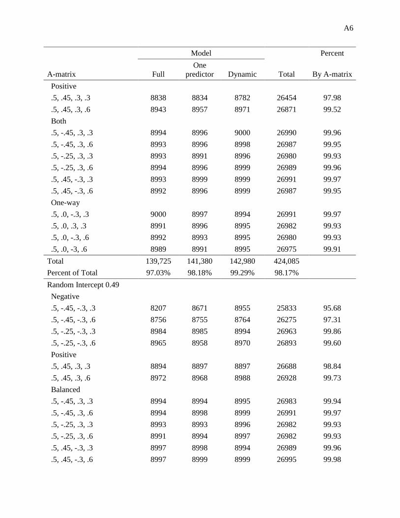
A6

Model Percent

A-matrix Full One

predictor Dynamic Total By A-matrix Positive .5, .45, .3, .3 8838 8834 8782 26454 97.98 .5, .45, .3, .6 8943 8957 8971 26871 99.52 Both .5, -.45, .3, .3 8994 8996 9000 26990 99.96 .5, -.45, .3, .6 8993 8996 8998 26987 99.95 .5, -.25, .3, .3 8993 8991 8996 26980 99.93 .5, -.25, .3, .6 8994 8996 8999 26989 99.96 .5, .45, -.3, .3 8993 8999 8999 26991 99.97 .5, .45, -.3, .6 8992 8996 8999 26987 99.95 One-way .5, .0, -.3, .3 9000 8997 8994 26991 99.97 .5, .0, .3, .3 8991 8996 8995 26982 99.93 .5, .0, -.3, .6 8992 8993 8995 26980 99.93 .5, .0, -3, .6 8989 8991 8995 26975 99.91 Total 139,725 141,380 142,980 424,085 Percent of Total 97.03% 98.18% 99.29% 98.17% Random Intercept 0.49 Negative .5, -.45, -.3, .3 8207 8671 8955 25833 95.68 .5, -.45, -.3, .6 8756 8755 8764 26275 97.31 .5, -.25, -.3, .3 8984 8985 8994 26963 99.86 .5, -.25, -.3, .6 8965 8958 8970 26893 99.60 Positive .5, .45, .3, .3 8894 8897 8897 26688 98.84 .5, .45, .3, .6 8972 8968 8988 26928 99.73 Balanced .5, -.45, .3, .3 8994 8994 8995 26983 99.94 .5, -.45, .3, .6 8994 8998 8999 26991 99.97 .5, -.25, .3, .3 8993 8993 8996 26982 99.93 .5, -.25, .3, .6 8991 8994 8997 26982 99.93 .5, .45, -.3, .3 8997 8998 8994 26989 99.96 .5, .45, -.3, .6 8997 8999 8999 26995 99.98

A7

Model Percent

A-matrix Full One

predictor Dynamic Total By A-matrix One-way .5, .0, -.3, .3 8995 8990 8999 26984 99.94 .5, .0, .3, .3 8989 8994 8990 26973 99.90 .5, .0, -.3, .6 8996 8991 8999 26986 99.95 .5, .0, -3, .6 8991 8991 8998 26980 99.93 Total 142,715 143,176 143,534 429,425 Percent of Total 99.11% 99.43% 99.68% 99.40%

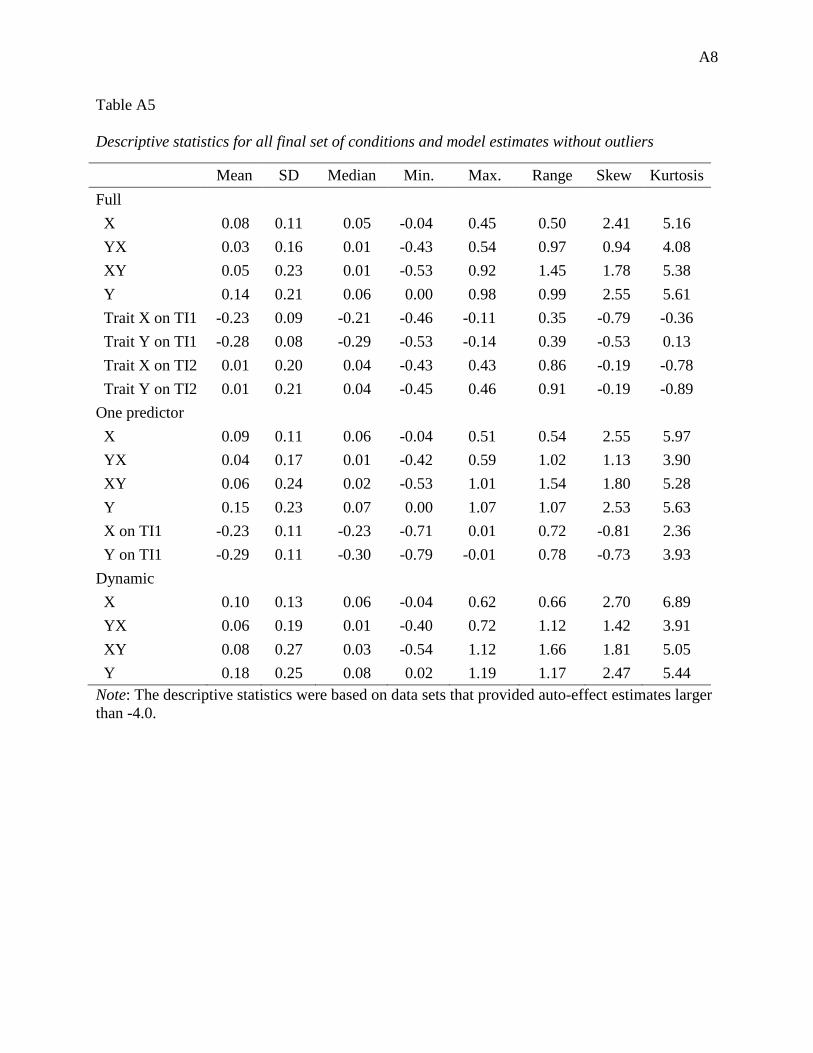
A8

Table A5

Descriptive statistics for all final set of conditions and model estimates without outliers

Mean SD Median Min. Max. Range Skew Kurtosis

Full

X 0.08 0.11 0.05 -0.04 0.45 0.50 2.41 5.16 YX 0.03 0.16 0.01 -0.43 0.54 0.97 0.94 4.08 XY 0.05 0.23 0.01 -0.53 0.92 1.45 1.78 5.38 Y 0.14 0.21 0.06 0.00 0.98 0.99 2.55 5.61 Trait X on TI1 -0.23 0.09 -0.21 -0.46 -0.11 0.35 -0.79 -0.36 Trait Y on TI1 -0.28 0.08 -0.29 -0.53 -0.14 0.39 -0.53 0.13 Trait X on TI2 0.01 0.20 0.04 -0.43 0.43 0.86 -0.19 -0.78 Trait Y on TI2 0.01 0.21 0.04 -0.45 0.46 0.91 -0.19 -0.89 One predictor

X 0.09 0.11 0.06 -0.04 0.51 0.54 2.55 5.97 YX 0.04 0.17 0.01 -0.42 0.59 1.02 1.13 3.90 XY 0.06 0.24 0.02 -0.53 1.01 1.54 1.80 5.28 Y 0.15 0.23 0.07 0.00 1.07 1.07 2.53 5.63 X on TI1 -0.23 0.11 -0.23 -0.71 0.01 0.72 -0.81 2.36 Y on TI1 -0.29 0.11 -0.30 -0.79 -0.01 0.78 -0.73 3.93 Dynamic

X 0.10 0.13 0.06 -0.04 0.62 0.66 2.70 6.89 YX 0.06 0.19 0.01 -0.40 0.72 1.12 1.42 3.91 XY 0.08 0.27 0.03 -0.54 1.12 1.66 1.81 5.05 Y 0.18 0.25 0.08 0.02 1.19 1.17 2.47 5.44 Note: The descriptive statistics were based on data sets that provided auto-effect estimates larger than -4.0.

A9

Table A6

Average bias of X auto-effect estimates for full, one predictor, and dynamic models

Full

One predictor

Dynamic

True value Mean SD

Mean SD

Mean SD

Random intercept r = 0

Balanced

.5, -.45, .3, .3 -0.42 0.04 0.01

0.04 0.01

0.05 0.01 .5, -.45, .3, .6 -0.50 0.04 0.00

0.04 0.00

0.04 0.01

.5, -.25, .3, .3 -0.52 0.03 0.01

0.04 0.01

0.05 0.01 .5, -.25, .3, .6 -0.57 0.05 0.00

0.06 0.00

0.07 0.00

.5, .45, -.3, .3 -0.42 0.06 0.00

0.06 0.00

0.06 0.00 .5, .45, -.3, .6 -0.50 0.06 0.00

0.06 0.00

0.06 0.00

One-way

.5, .0, -.3, .3 -0.69 0.04 0.00

0.05 0.01

0.07 0.01 .5, .0, .3, .3 -0.69 0.04 0.00

0.05 0.01

0.06 0.01

.5, .0, -.3, .6 -0.69 0.05 0.00

0.06 0.01

0.07 0.01 .5, .0, .3, .6 -0.69 0.06 0.00

0.06 0.01

0.07 0.01

Positive

.5, .45, .3, .3 -1.61 0.23 0.06

0.23 0.06

0.23 0.05 .5, .45, .3, .6 -1.01 -0.02 0.00

-0.02 0.00

-0.03 0.00

Negative

.5, -.45, -.3, .3 -1.61 0.43 0.02

0.47 0.03

0.55 0.04 .5, -.45, -.3, .6 -1.01 -0.02 0.01

0.01 0.02

0.05 0.03

.5, -.25, -.3, .3 -0.98 0.08 0.01

0.11 0.02

0.15 0.02 .5, -.25, -.3, .6 -0.85 0.06 0.00

0.08 0.01

0.10 0.01

A10

Table A7

Average bias of Y auto-effect estimates for full, one predictor, and dynamic models

Full

One predictor

Dynamic

True value Mean SD

Mean SD

Mean SD

Random intercept r = 0

Balanced

.5, -.45, .3, .3 -0.83 0.05 0.01

0.06 0.01

0.06 0.01 .5, -.45, .3, .6 -0.34 0.04 0.01

0.04 0.01

0.04 0.01

.5, -.25, .3, .3 -0.97 0.10 0.02

0.10 0.02

0.10 0.02 .5, -.25, .3, .6 -0.41 0.05 0.01

0.05 0.01

0.05 0.01

.5, .45, -.3, .3 -0.83 0.01 0.01

0.02 0.01

0.03 0.00 .5, .45, -.3, .6 -0.34 0.02 0.00

0.02 0.00

0.03 0.00

One-way

.5, .0, -.3, .3 -1.20 0.12 0.03

0.14 0.03

0.17 0.03 .5, .0, .3, .3 -1.20 0.12 0.02

0.13 0.02

0.14 0.02

.5, .0, -.3, .6 -0.51 0.03 0.02

0.05 0.02

0.07 0.02 .5, .0, .3, .6 -0.51 0.05 0.01

0.05 0.01

0.05 0.01

Positive

.5, .45, .3, .3 -2.59 0.44 0.16

0.46 0.16

0.50 0.14 .5, .45, .3, .6 -0.79 0.05 0.02

0.05 0.02

0.05 0.02

Negative

.5, -.45, -.3, .3 -2.59 0.84 0.09

0.89 0.11

1.01 0.11 .5, -.45, -.3, .6 -0.79 0.09 0.04

0.11 0.04

0.15 0.04

.5, -.25, -.3, .3 -1.61 0.21 0.08

0.26 0.08

0.34 0.06 .5, -.25, -.3, .6 -0.65 0.04 0.03

0.05 0.03

0.07 0.02

A11

Table A8

Average bias of YX cross-effect estimates for full, one predictor, and dynamic models

Full

One predictor

Dynamic

True value Mean SD

Mean SD

Mean SD

Random intercept r = 0

Balanced

.5, -.45, .3, .3 0.61 -0.01 0.00

-0.01 0.00

-0.01 0.00 .5, -.45, .3, .6 0.48 0.00 0.00

0.00 0.00

0.00 0.00

.5, -.25, .3, .3 0.67 -0.01 0.00

-0.01 0.00

0.00 0.00 .5, -.25, .3, .6 0.51 0.01 0.00

0.01 0.00

0.01 0.00

.5, .45, -.3, .3 -0.61 0.02 0.00

0.02 0.01

0.04 0.01 .5, .45, -.3, .6 -0.48 0.00 0.00

0.00 0.00

0.01 0.00

One-way

.5, .0, -.3, .3 -0.77 0.06 0.00

0.08 0.01

0.10 0.01 .5, .0, .3, .3 0.77 -0.04 0.00

-0.04 0.01

-0.03 0.01

.5, .0, -.3, .6 -0.55 0.02 0.00

0.03 0.01

0.04 0.01 .5, .0, .3, .6 0.55 0.00 0.00

0.00 0.00

0.01 0.00

Positive

.5, .45, .3, .3 1.46 -0.33 0.07

-0.32 0.07

-0.31 0.06 .5, .45, .3, .6 0.66 -0.08 0.01

-0.08 0.01

-0.08 0.01

Negative

.5, -.45, -.3, .3 -1.46 0.50 0.03

0.55 0.04

0.63 0.05 .5, -.45, -.3, .6 -0.66 0.05 0.01

0.08 0.02

0.11 0.02

.5, -.25, -.3, .3 -0.95 0.17 0.01

0.20 0.03

0.25 0.02 .5, -.25, -.3, .6 -0.60 0.08 0.01

0.09 0.02

0.12 0.01

A12

Table A9

Average bias of XY cross-effect estimates for full, one predictor, and dynamic models

Full

One predictor

Dynamic

True value Mean SD

Mean SD

Mean SD

Random intercept r = 0

Balanced

.5, -.45, .3, .3 -0.92 0.01 0.02

0.02 0.02

0.03 0.02 .5, -.45, .3, .6 -0.72 0.00 0.01

0.00 0.02

0.01 0.01

.5, -.25, .3, .3 -0.56 0.01 0.02

0.02 0.02

0.04 0.02 .5, -.25, .3, .6 -0.42 -0.02 0.02

-0.01 0.02

0.00 0.01

.5, .45, -.3, .3 0.92 0.01 0.01

0.01 0.01

0.02 0.00 .5, .45, -.3, .6 0.72 0.00 0.00

0.00 0.00

0.00 0.00

One-way

.5, .0, -.3, .3 0.00 0.01 0.01

0.02 0.01

0.04 0.01 .5, .0, .3, .3 0.00 0.00 0.01

0.01 0.01

0.03 0.01

.5, .0, -.3, .6 0.00 0.02 0.00

0.03 0.01

0.05 0.01 .5, .0, .3, .6 0.00 -0.06 0.01

-0.05 0.01

-0.04 0.01

Positive

.5, .45, .3, .3 2.19 -0.34 0.14

-0.35 0.13

-0.38 0.11 .5, .45, .3, .6 0.99 -0.16 0.02

-0.16 0.01

-0.16 0.01

Negative

.5, -.45, -.3, .3 -2.19 0.79 0.09

0.84 0.10

0.95 0.10 .5, -.45, -.3, .6 -0.99 0.24 0.05

0.26 0.05

0.30 0.04

.5, -.25, -.3, .3 -0.79 0.10 0.05

0.14 0.05

0.20 0.04 .5, -.25, -.3, .6 -0.50 0.11 0.02

0.12 0.02

0.15 0.02

A13

Table A10

Average bias of time-invariant effect on X trait variance for full and one predictor

Full

One predictor

True value Mean SD

Mean SD

Random intercept r = 0

Balanced

.5, -.45, .3, .3 0.55 -0.11 0.00

-0.12 0.08 .5, -.45, .3, .6 0.52 -0.13 0.00

-0.13 0.07

.5, -.25, .3, .3 0.50 -0.16 0.01

-0.17 0.06 .5, -.25, .3, .6 0.48 -0.16 0.01

-0.17 0.06

.5, .45, -.3, .3 0.16 -0.38 0.00

-0.38 0.04 .5, .45, -.3, .6 0.23 -0.35 0.00

-0.35 0.02

One-way

.5, .0, -.3, .3 0.42 -0.22 0.00

-0.23 0.04 .5, .0, .3, .3 0.42 -0.22 0.00

-0.23 0.04

.5, .0, -.3, .6 0.42 -0.23 0.00

-0.24 0.04 .5, .0, .3, .6 0.42 -0.20 0.00

-0.21 0.04

Positive

.5, .45, .3, .3 0.06 -0.29 0.03

-0.29 0.04 .5, .45, .3, .6 0.27 -0.25 0.01

-0.25 0.01

Negative

.5, -.45, -.3, .3 1.26 -0.41 0.03

-0.45 0.16 .5, -.45, -.3, .6 0.72 -0.14 0.01

-0.16 0.11

.5, -.25, -.3, .3 0.68 -0.17 0.02

-0.19 0.09 .5, -.25, -.3, .6 0.56 -0.19 0.01

-0.20 0.07

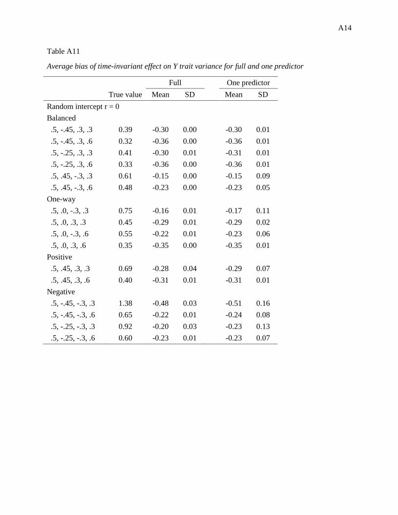
A14

Table A11

Average bias of time-invariant effect on Y trait variance for full and one predictor

Full

One predictor

True value Mean SD

Mean SD

Random intercept r = 0

Balanced

.5, -.45, .3, .3 0.39 -0.30 0.00

-0.30 0.01 .5, -.45, .3, .6 0.32 -0.36 0.00

-0.36 0.01

.5, -.25, .3, .3 0.41 -0.30 0.01

-0.31 0.01 .5, -.25, .3, .6 0.33 -0.36 0.00

-0.36 0.01

.5, .45, -.3, .3 0.61 -0.15 0.00

-0.15 0.09 .5, .45, -.3, .6 0.48 -0.23 0.00

-0.23 0.05

One-way

.5, .0, -.3, .3 0.75 -0.16 0.01

-0.17 0.11 .5, .0, .3, .3 0.45 -0.29 0.01

-0.29 0.02

.5, .0, -.3, .6 0.55 -0.22 0.01

-0.23 0.06 .5, .0, .3, .6 0.35 -0.35 0.00

-0.35 0.01

Positive

.5, .45, .3, .3 0.69 -0.28 0.04

-0.29 0.07 .5, .45, .3, .6 0.40 -0.31 0.01

-0.31 0.01

Negative

.5, -.45, -.3, .3 1.38 -0.48 0.03

-0.51 0.16 .5, -.45, -.3, .6 0.65 -0.22 0.01

-0.24 0.08

.5, -.25, -.3, .3 0.92 -0.20 0.03

-0.23 0.13 .5, -.25, -.3, .6 0.60 -0.23 0.01

-0.23 0.07

A15

Table A12

X auto-effect relative bias for comparison of full to omitted variable models averaged over A-matrix simulation conditions

Full / One Predictor Full / Dynamic With

Outliers Without Outliers

With Outliers

Without Outliers

Balanced

.5, -.45, .3, .3 0.81 0.88

0.69 0.74 .5, -.45, .3, .6 0.91 0.91

0.82 0.82

.5, -.25, .3, .3 0.84 0.82

0.66 0.64 .5, -.25, .3, .6 0.91 0.91

0.79 0.80

.5, .45, -.3, .3 1.02 1.02

1.07 1.07 .5, .45, -.3, .6 0.96 1.01

0.96 1.01

One-way

.5, .0, -.3, .3 0.86 0.84

0.66 0.67 .5, .0, .3, .3 0.81 0.85

0.66 0.70

.5, .0, -.3, .6 0.89 0.89

0.76 0.76 .5, .0, .3, .6 0.89 0.89

0.77 0.77

Positive

.5, .45, .3, .3 1.34 1.01

0.28 1.01 .5, .45, .3, .6 0.96 0.96

0.84 0.84

Negative

.5, -.45, -.3, .3 6.21 0.91

-14.70 0.78 .5, -.45, -.3, .6 1.19 -4.65

-0.29 -0.94

.5, -.25, -.3, .3 0.05 0.76

-3.84 0.55 .5, -.25, -.3, .6 1.06 0.81

-0.65 0.62

Note. Relative bias greater than 1 indicates that the omitted model was less biased than the full model. Relative bias less than 1 indicates that the full model was less biased than the omitted variable model.

A16

Table A13

Y auto-effect relative bias for comparison of full to omitted variable models averaged over A-matrix simulation conditions

Full / One Predictor Full / Dynamic With

Outliers Without Outliers

With Outliers

Without Outliers

Balanced

.5, -.45, .3, .3 1.04 0.99

0.99 0.95 .5, -.45, .3, .6 0.99 0.99

0.96 0.96

.5, -.25, .3, .3 0.95 0.97

0.91 0.93 .5, -.25, .3, .6 0.99 0.99

0.99 0.96

.5, .45, -.3, .3 0.60 0.60

0.47 0.47 .5, .45, -.3, .6 1.03 0.87

0.85 0.74

One-way

.5, .0, -.3, .3 0.84 0.85

0.68 0.68 .5, .0, .3, .3 -1.04 0.95

-1.04 0.87

.5, .0, -.3, .6 0.67 0.67

0.42 0.42 .5, .0, .3, .6 0.98 0.98

0.93 0.93

Positive

.5, .45, .3, .3 1.09 0.95

1.12 0.86 .5, .45, .3, .6 1.08 1.08

1.12 1.12

Negative

.5, -.45, -.3, .3 12.90 0.94

-1101.26 0.84 .5, -.45, -.3, .6 1.03 0.77

-0.85 0.54

.5, -.25, -.3, .3 7.54 0.81

7.27 0.61 .5, -.25, -.3, .6 0.85 0.70

-1.08 0.44

Note. Relative bias greater than 1 indicates that the omitted model was less biased than the full model. Relative bias less than 1 indicates that the full model was less biased than the omitted variable model.

A17

Table A14

YX cross-effect relative bias for comparison of full to omitted variable models averaged over A-matrix simulation conditions

Full / One Predictor Full / Dynamic With

Outliers Without Outliers

With Outliers

Without Outliers

Balanced

.5, -.45, .3, .3 1.59 1.12

2.09 1.59 .5, -.45, .3, .6 4.67 4.67

-0.52 -0.52

.5, -.25, .3, .3 1.09 1.43

0.87 1.17 .5, -.25, .3, .6 0.94 0.94

0.82 0.84

.5, .45, -.3, .3 0.74 0.74

0.50 0.50 .5, .45, -.3, .6 3.73 0.04

-2.95 -0.69

One-way

.5, .0, -.3, .3 0.83 0.79

0.58 0.58 .5, .0, .3, .3 -2.39 1.12

-2.64 1.39

.5, .0, -.3, .6 0.75 0.75

0.54 0.53 .5, .0, .3, .6 0.74 0.74

0.42 0.42

Positive

.5, .45, .3, .3 1.18 1.03

1.28 1.07 .5, .45, .3, .6 0.98 0.98

1.01 1.01

Negative

.5, -.45, -.3, .3 6.72 0.92

15.93 0.80 .5, -.45, -.3, .6 1.17 0.72

-31.96 0.48

.5, -.25, -.3, .3 0.06 0.83

-1.33 0.66 .5, -.25, -.3, .6 1.32 0.83

-0.27 0.67

Note. Relative bias greater than 1 indicates that the omitted model was less biased than the full model. Relative bias less than 1 indicates that the full model was less biased than the omitted variable model.

A18

Table A15

XY cross-effect relative bias for comparison of full to omitted variable models averaged over A-matrix simulation conditions

Full / One Predictor Full / Dynamic With

Outliers Without Outliers

With Outliers

Without Outliers

Balanced

.5, -.45, .3, .3 0.58 0.40

0.42 0.15 .5, -.45, .3, .6 2.16 2.16

2.33 2.33

.5, -.25, .3, .3 0.24 -0.11

-0.17 0.07 .5, -.25, .3, .6 1.12 1.12

1.16 1.36

.5, .45, -.3, .3 0.69 0.69

0.61 0.61 .5, .45, -.3, .6 -1.46 0.19

4.89 -0.68

One-way

.5, .0, -.3, .3 0.56 0.57

0.29 0.29 .5, .0, .3, .3 0.25 0.11

0.04 -0.06

.5, .0, -.3, .6 0.71 0.71

0.46 0.46 .5, .0, .3, .6 1.12 1.12

1.43 1.43

Positive

.5, .45, .3, .3 1.63 0.96

0.74 0.87 .5, .45, .3, .6 0.99 0.99

0.98 0.98

Negative

.5, -.45, -.3, .3 11.54 0.94

-39.53 0.83 .5, -.45, -.3, .6 0.64 0.90

-1.07 0.77

.5, -.25, -.3, .3 -11.00 0.71

2.40 0.47 .5, -.25, -.3, .6 1.68 0.90

0.11 0.74

Note. Relative bias greater than 1 indicates that the omitted model was less biased than the full model. Relative bias less than 1 indicates that the full model was less biased than the omitted variable model.

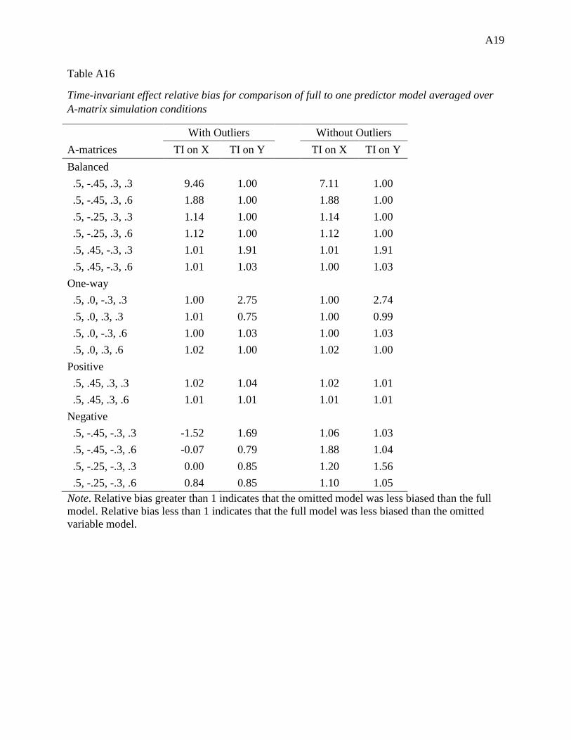
A19

Table A16

Time-invariant effect relative bias for comparison of full to one predictor model averaged over A-matrix simulation conditions

With Outliers

Without Outliers

A-matrices TI on X TI on Y

TI on X TI on Y Balanced

.5, -.45, .3, .3 9.46 1.00

7.11 1.00 .5, -.45, .3, .6 1.88 1.00

1.88 1.00

.5, -.25, .3, .3 1.14 1.00

1.14 1.00 .5, -.25, .3, .6 1.12 1.00

1.12 1.00

.5, .45, -.3, .3 1.01 1.91

1.01 1.91 .5, .45, -.3, .6 1.01 1.03

1.00 1.03

One-way

.5, .0, -.3, .3 1.00 2.75

1.00 2.74 .5, .0, .3, .3 1.01 0.75

1.00 0.99

.5, .0, -.3, .6 1.00 1.03

1.00 1.03 .5, .0, .3, .6 1.02 1.00

1.02 1.00

Positive

.5, .45, .3, .3 1.02 1.04

1.02 1.01 .5, .45, .3, .6 1.01 1.01

1.01 1.01

Negative

.5, -.45, -.3, .3 -1.52 1.69

1.06 1.03 .5, -.45, -.3, .6 -0.07 0.79

1.88 1.04

.5, -.25, -.3, .3 0.00 0.85

1.20 1.56 .5, -.25, -.3, .6 0.84 0.85

1.10 1.05

Note. Relative bias greater than 1 indicates that the omitted model was less biased than the full model. Relative bias less than 1 indicates that the full model was less biased than the omitted variable model.

A20

Table A17

X auto-effect relative efficiency for comparison of full to omitted variable models averaged over A-matrix simulation conditions

Full / One Predictor Full / Dynamic With

Outliers Without Outliers

With Outliers

Without Outliers

Balanced

.5, -.45, .3, .3 3.24 0.80

12.19 0.43 .5, -.45, .3, .6 0.80 0.80

0.40 0.40

.5, -.25, .3, .3 4.63 0.95

3.99 0.21 .5, -.25, .3, .6 1.12 1.12

0.24 0.24

.5, .45, -.3, .3 0.38 0.38

0.04 0.04 .5, .45, -.3, .6 4.15 0.46

1.87 0.04

One-way

.5, .0, -.3, .3 0.90 0.90

0.10 0.10 .5, .0, .3, .3 1.85 0.82

1.57 0.09

.5, .0, -.3, .6 1.08 1.08

0.11 0.11 .5, .0, .3, .6 1.14 1.14

0.14 0.14

Positive

.5, .45, .3, .3 21.17 4.26

4.64 1.10 .5, .45, .3, .6 0.89 0.89

0.14 0.14

Negative

.5, -.45, -.3, .3 17.21 8.24

27.12 1.25 .5, -.45, -.3, .6 33.54 1.75

3.82 0.65

.5, -.25, -.3, .3 15.29 2.36

3.70 0.58 .5, -.25, -.3, .6 3.64 1.43

148.31 0.28

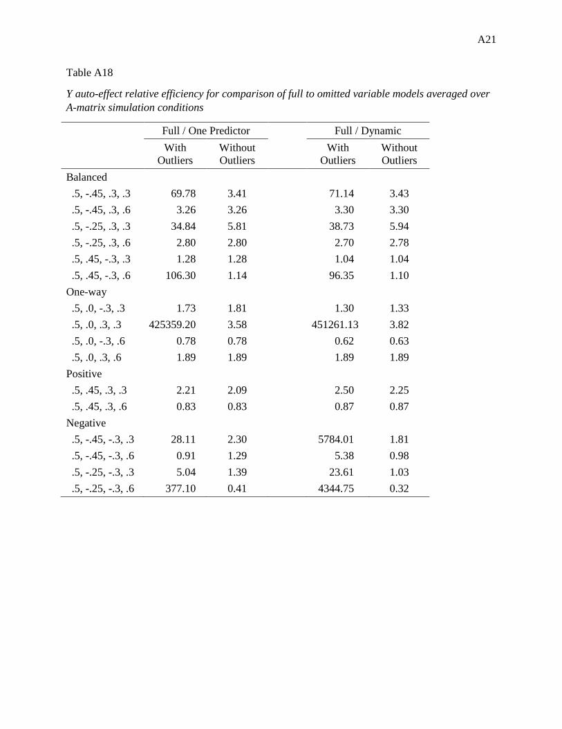
A21

Table A18

Y auto-effect relative efficiency for comparison of full to omitted variable models averaged over A-matrix simulation conditions

Full / One Predictor Full / Dynamic With

Outliers Without Outliers

With Outliers

Without Outliers

Balanced

.5, -.45, .3, .3 69.78 3.41

71.14 3.43 .5, -.45, .3, .6 3.26 3.26

3.30 3.30

.5, -.25, .3, .3 34.84 5.81

38.73 5.94 .5, -.25, .3, .6 2.80 2.80

2.70 2.78

.5, .45, -.3, .3 1.28 1.28

1.04 1.04 .5, .45, -.3, .6 106.30 1.14

96.35 1.10

One-way

.5, .0, -.3, .3 1.73 1.81

1.30 1.33 .5, .0, .3, .3 425359.20 3.58

451261.13 3.82

.5, .0, -.3, .6 0.78 0.78

0.62 0.63 .5, .0, .3, .6 1.89 1.89

1.89 1.89

Positive

.5, .45, .3, .3 2.21 2.09

2.50 2.25 .5, .45, .3, .6 0.83 0.83

0.87 0.87

Negative

.5, -.45, -.3, .3 28.11 2.30

5784.01 1.81 .5, -.45, -.3, .6 0.91 1.29

5.38 0.98

.5, -.25, -.3, .3 5.04 1.39

23.61 1.03 .5, -.25, -.3, .6 377.10 0.41

4344.75 0.32

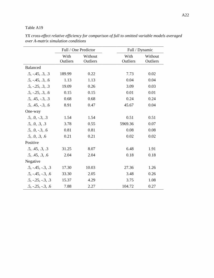
A22

Table A19

YX cross-effect relative efficiency for comparison of full to omitted variable models averaged over A-matrix simulation conditions

Full / One Predictor Full / Dynamic With

Outliers Without Outliers

With Outliers

Without Outliers

Balanced

.5, -.45, .3, .3 189.99 0.22

7.73 0.02 .5, -.45, .3, .6 1.13 1.13

0.04 0.04

.5, -.25, .3, .3 19.09 0.26

3.09 0.03 .5, -.25, .3, .6 0.15 0.15

0.01 0.01

.5, .45, -.3, .3 0.68 0.68

0.24 0.24 .5, .45, -.3, .6 8.91 0.47

45.67 0.04

One-way

.5, .0, -.3, .3 1.54 1.54

0.51 0.51 .5, .0, .3, .3 3.78 0.55

5969.36 0.07

.5, .0, -.3, .6 0.81 0.81

0.08 0.08 .5, .0, .3, .6 0.21 0.21

0.02 0.02

Positive

.5, .45, .3, .3 31.25 8.07

6.48 1.91 .5, .45, .3, .6 2.04 2.04

0.18 0.18

Negative

.5, -.45, -.3, .3 17.30 10.03

27.36 1.26 .5, -.45, -.3, .6 33.30 2.05

3.48 0.26

.5, -.25, -.3, .3 15.37 4.29

3.75 1.08 .5, -.25, -.3, .6 7.88 2.27

104.72 0.27

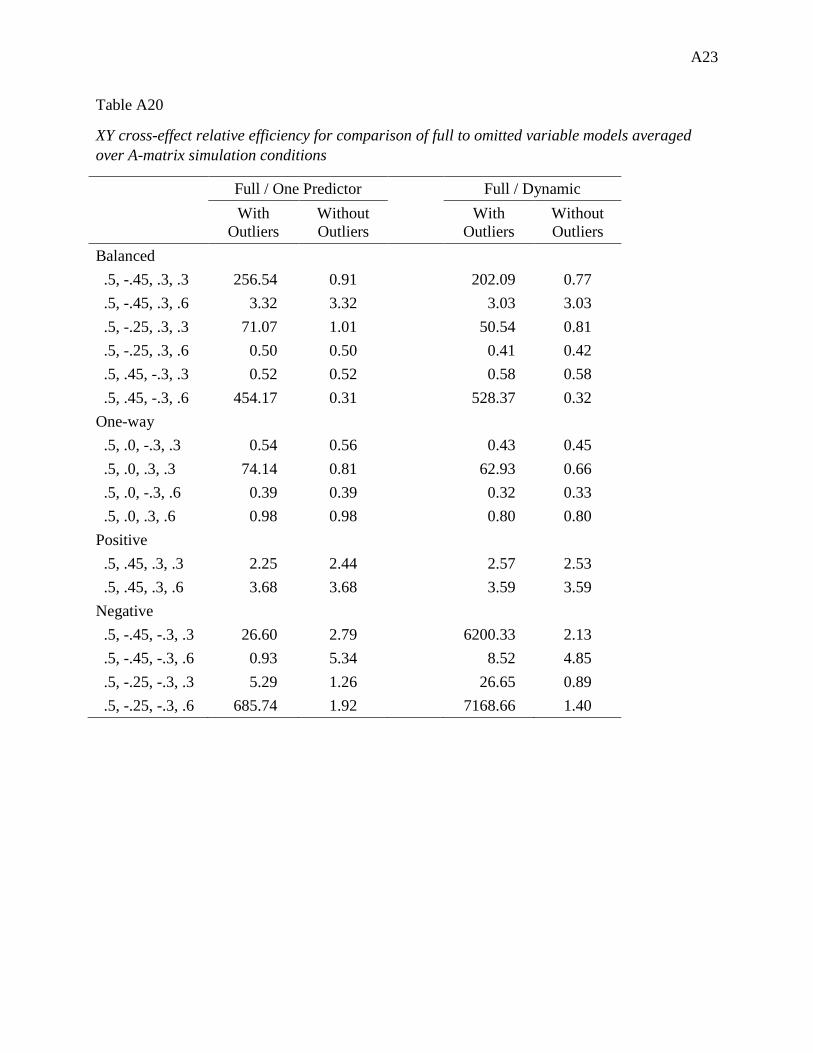
A23

Table A20

XY cross-effect relative efficiency for comparison of full to omitted variable models averaged over A-matrix simulation conditions

Full / One Predictor Full / Dynamic With

Outliers Without Outliers

With Outliers

Without Outliers

Balanced

.5, -.45, .3, .3 256.54 0.91

202.09 0.77 .5, -.45, .3, .6 3.32 3.32

3.03 3.03

.5, -.25, .3, .3 71.07 1.01

50.54 0.81 .5, -.25, .3, .6 0.50 0.50

0.41 0.42

.5, .45, -.3, .3 0.52 0.52

0.58 0.58 .5, .45, -.3, .6 454.17 0.31

528.37 0.32

One-way

.5, .0, -.3, .3 0.54 0.56

0.43 0.45 .5, .0, .3, .3 74.14 0.81

62.93 0.66

.5, .0, -.3, .6 0.39 0.39

0.32 0.33 .5, .0, .3, .6 0.98 0.98

0.80 0.80

Positive

.5, .45, .3, .3 2.25 2.44

2.57 2.53 .5, .45, .3, .6 3.68 3.68

3.59 3.59

Negative

.5, -.45, -.3, .3 26.60 2.79

6200.33 2.13 .5, -.45, -.3, .6 0.93 5.34

8.52 4.85

.5, -.25, -.3, .3 5.29 1.26

26.65 0.89 .5, -.25, -.3, .6 685.74 1.92

7168.66 1.40

A24

Table A21

Time-invariant effect relative efficiency for comparison of full to one predictor model averaged over A-matrix simulation conditions

With Outliers Without Outliers TI on X trait

variance TI on Y trait

variance TI on X trait

variance TI on Y trait

variance Balanced

.5, -.45, .3, .3 14.53 17.68

3.99 15.08

.5, -.45, .3, .6 7.63 47.10

7.63 47.10 .5, -.25, .3, .3 9.09 6.75

5.38 6.75

.5, -.25, .3, .6 10.23 34.95

10.23 34.95 .5, .45, -.3, .3 72.12 5.72

72.12 5.72

.5, .45, -.3, .6 195.11 29.23

95.11 19.54 One-way

.5, .0, -.3, .3 14.08 1.10

14.60 1.13

.5, .0, .3, .3 16.36 4698.45

11.55 4.19 .5, .0, -.3, .6 17.35 12.03

17.35 12.03

.5, .0, .3, .6 7.57 35.44

7.57 35.44 Positive

.5, .45, .3, .3 0.11 0.08

0.46 0.27

.5, .45, .3, .6 1.99 7.24

1.99 7.24 Negative

.5, -.45, -.3, .3 4.78 4.91

0.25 0.30

.5, -.45, -.3, .6 0.60 0.63

0.32 2.51 .5, -.25, -.3, .3 1.02 0.83

1.08 0.56

.5, -.25, -.3, .6 254.72 667.01 1.77 8.42

B1

Appendix B: Supplementary Simulation 2 Tables

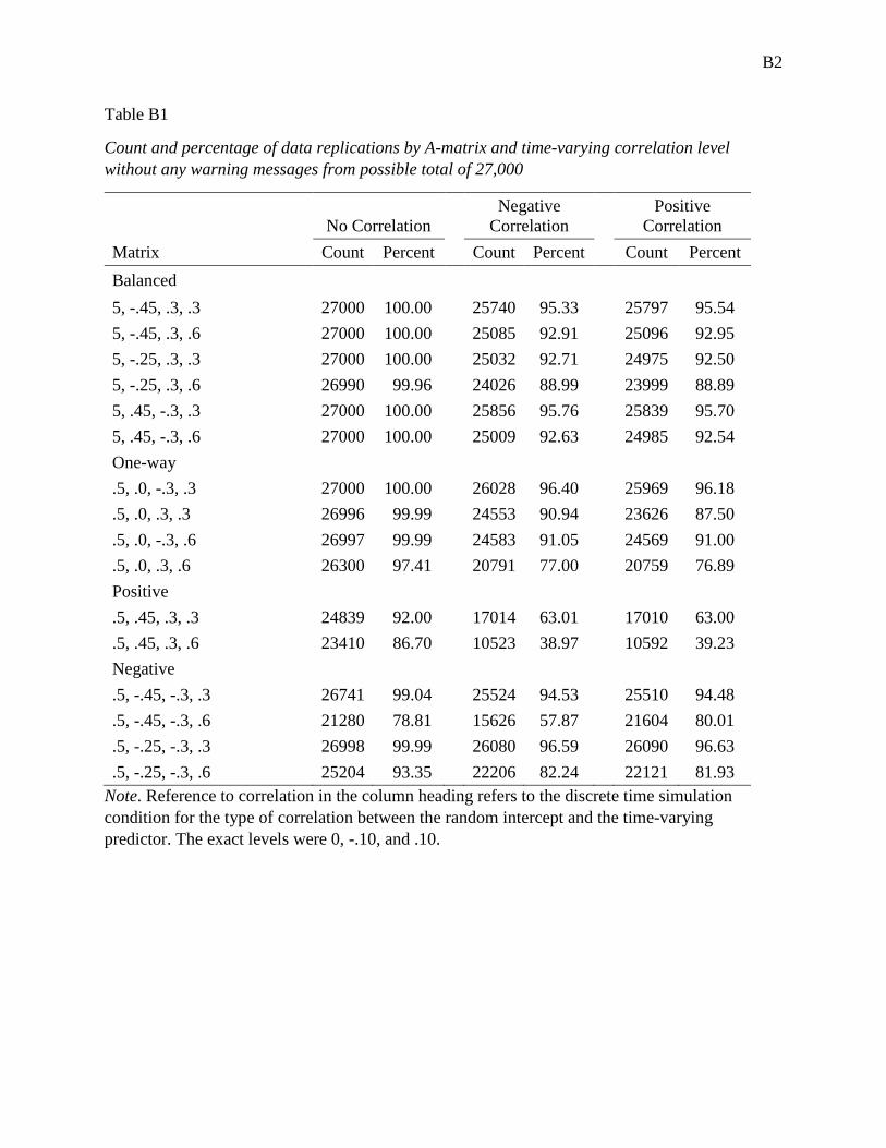
B2

Table B1

Count and percentage of data replications by A-matrix and time-varying correlation level without any warning messages from possible total of 27,000

No Correlation Negative

Correlation Positive

Correlation Matrix Count Percent Count Percent Count Percent Balanced 5, -.45, .3, .3 27000 100.00 25740 95.33 25797 95.54 5, -.45, .3, .6 27000 100.00 25085 92.91 25096 92.95 5, -.25, .3, .3 27000 100.00 25032 92.71 24975 92.50 5, -.25, .3, .6 26990 99.96 24026 88.99 23999 88.89 5, .45, -.3, .3 27000 100.00 25856 95.76 25839 95.70 5, .45, -.3, .6 27000 100.00 25009 92.63 24985 92.54 One-way .5, .0, -.3, .3 27000 100.00 26028 96.40 25969 96.18 .5, .0, .3, .3 26996 99.99 24553 90.94 23626 87.50 .5, .0, -.3, .6 26997 99.99 24583 91.05 24569 91.00 .5, .0, .3, .6 26300 97.41 20791 77.00 20759 76.89 Positive .5, .45, .3, .3 24839 92.00 17014 63.01 17010 63.00 .5, .45, .3, .6 23410 86.70 10523 38.97 10592 39.23 Negative .5, -.45, -.3, .3 26741 99.04 25524 94.53 25510 94.48 .5, -.45, -.3, .6 21280 78.81 15626 57.87 21604 80.01 .5, -.25, -.3, .3 26998 99.99 26080 96.59 26090 96.63 .5, -.25, -.3, .6 25204 93.35 22206 82.24 22121 81.93

Note. Reference to correlation in the column heading refers to the discrete time simulation condition for the type of correlation between the random intercept and the time-varying predictor. The exact levels were 0, -.10, and .10.

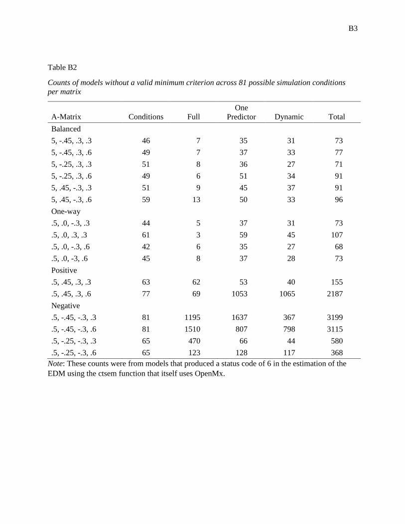
B3

Table B2

Counts of models without a valid minimum criterion across 81 possible simulation conditions per matrix

A-Matrix Conditions Full One

Predictor Dynamic Total Balanced 5, -.45, .3, .3 46 7 35 31 73 5, -.45, .3, .6 49 7 37 33 77 5, -.25, .3, .3 51 8 36 27 71 5, -.25, .3, .6 49 6 51 34 91 5, .45, -.3, .3 51 9 45 37 91 5, .45, -.3, .6 59 13 50 33 96 One-way .5, .0, -.3, .3 44 5 37 31 73 .5, .0, .3, .3 61 3 59 45 107 .5, .0, -.3, .6 42 6 35 27 68 .5, .0, -3, .6 45 8 37 28 73 Positive .5, .45, .3, .3 63 62 53 40 155 .5, .45, .3, .6 77 69 1053 1065 2187 Negative .5, -.45, -.3, .3 81 1195 1637 367 3199 .5, -.45, -.3, .6 81 1510 807 798 3115 .5, -.25, -.3, .3 65 470 66 44 580 .5, -.25, -.3, .6 65 123 128 117 368

Note: These counts were from models that produced a status code of 6 in the estimation of the EDM using the ctsem function that itself uses OpenMx.

B4

Table B3

Descriptive statistics of bias across all 1296 simulation conditions with all converged models

Mean SD Median Min. Max. Range Skew Kurtosis Full

X -0.06 1.09 0.05 -25.52 0.58 26.10 -15.17 286.87 YX -0.11 1.18 0.00 -27.78 0.70 28.48 -15.32 294.33 XY -0.14 1.66 0.01 -39.81 1.16 40.98 -15.50 303.45 Y -0.07 1.81 0.05 -43.46 1.25 44.71 -15.65 309.12 Trait X on TI1 -0.40 0.67 -0.32 -15.87 3.58 19.46 -12.57 273.08 Trait Y on TI1 -0.49 0.72 -0.37 -17.30 3.84 21.14 -12.81 282.07 One predictor

X -1.22 8.07 0.05 -87.01 0.86 87.87 -8.06 68.91 YX -0.31 38.96 -0.01 -94.36 1366.22 1460.57 33.19 1164.58 XY -1.94 12.60 0.00 -137.09 1.21 138.30 -8.20 71.41 Y -4.17 79.65 0.05 -2827.49 1.31 2828.80 -34.40 1215.03 X on TI1 0.41 6.74 -0.31 -18.70 75.55 94.24 8.78 81.32 Y on TI1 0.42 7.32 -0.37 -20.32 81.24 101.57 8.64 79.02 Dynamic

X -0.26 1.81 0.05 -18.61 1.01 19.62 -6.89 50.97 YX 2.35 89.21 0.00 -19.93 3198.93 3218.86 35.52 1268.92 XY -0.45 2.76 0.02 -28.06 1.23 29.30 -6.94 51.55 Y -5.51 171.56 0.06 -6158.71 1.34 6160.04 -35.61 1273.80

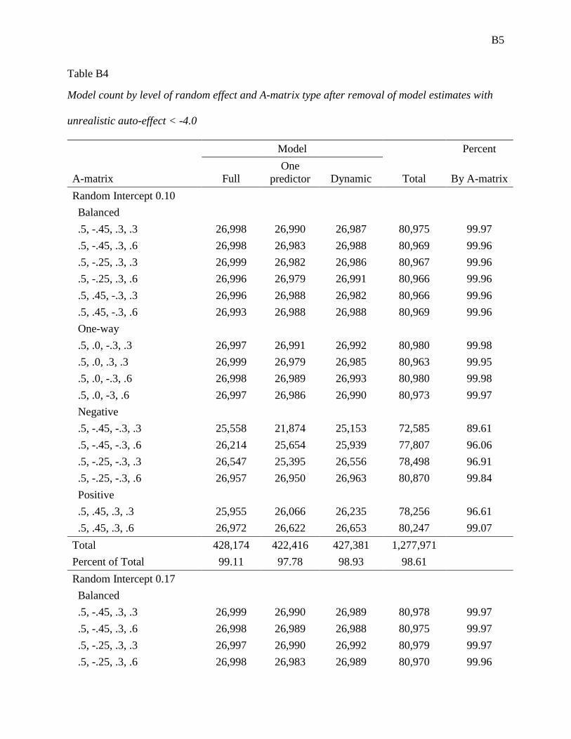
B5

Table B4

Model count by level of random effect and A-matrix type after removal of model estimates with

unrealistic auto-effect < -4.0

Model Percent

A-matrix Full One

predictor Dynamic Total By A-matrix Random Intercept 0.10 Balanced .5, -.45, .3, .3 26,998 26,990 26,987 80,975 99.97 .5, -.45, .3, .6 26,998 26,983 26,988 80,969 99.96 .5, -.25, .3, .3 26,999 26,982 26,986 80,967 99.96 .5, -.25, .3, .6 26,996 26,979 26,991 80,966 99.96 .5, .45, -.3, .3 26,996 26,988 26,982 80,966 99.96 .5, .45, -.3, .6 26,993 26,988 26,988 80,969 99.96 One-way .5, .0, -.3, .3 26,997 26,991 26,992 80,980 99.98 .5, .0, .3, .3 26,999 26,979 26,985 80,963 99.95 .5, .0, -.3, .6 26,998 26,989 26,993 80,980 99.98 .5, .0, -3, .6 26,997 26,986 26,990 80,973 99.97 Negative .5, -.45, -.3, .3 25,558 21,874 25,153 72,585 89.61 .5, -.45, -.3, .6 26,214 25,654 25,939 77,807 96.06 .5, -.25, -.3, .3 26,547 25,395 26,556 78,498 96.91 .5, -.25, -.3, .6 26,957 26,950 26,963 80,870 99.84 Positive .5, .45, .3, .3 25,955 26,066 26,235 78,256 96.61 .5, .45, .3, .6 26,972 26,622 26,653 80,247 99.07 Total 428,174 422,416 427,381 1,277,971 Percent of Total 99.11 97.78 98.93 98.61 Random Intercept 0.17 Balanced .5, -.45, .3, .3 26,999 26,990 26,989 80,978 99.97 .5, -.45, .3, .6 26,998 26,989 26,988 80,975 99.97 .5, -.25, .3, .3 26,997 26,990 26,992 80,979 99.97 .5, -.25, .3, .6 26,998 26,983 26,989 80,970 99.96

B6

Model Percent

A-matrix Full One

predictor Dynamic Total By A-matrix .5, .45, -.3, .3 26,999 26,983 26,988 80,970 99.96 .5, .45, -.3, .6 26,996 26,977 26,985 80,958 99.95 One-way .5, .0, -.3, .3 26,999 26,991 26,991 80,981 99.98 .5, .0, .3, .3 26,999 26,978 26,981 80,958 99.95 .5, .0, -.3, .6 26,998 26,991 26,991 80,980 99.98 .5, .0, -3, .6 26,997 26,986 26,992 80,975 99.97 Negative .5, -.45, -.3, .3 26,112 23,516 25,882 75,510 93.22 .5, -.45, -.3, .6 26,410 25,891 26,158 78,459 96.86 .5, -.25, -.3, .3 26,738 25,999 26,732 79,469 98.11 .5, -.25, -.3, .6 26,966 26,963 26,960 80,889 99.86 Positive .5, .45, .3, .3 26,465 26,612 26,636 79,713 98.41 .5, .45, .3, .6 26,973 26,675 26,694 80,342 99.19 Total 429,644 425,514 428,948 1,284,106 Percent of Total 99.45 98.50 99.29 99.08 Random Intercept 0.49 Balanced .5, -.45, .3, .3 26,996 26,985 26,989 80,970 99.96 .5, -.45, .3, .6 26,996 26,988 26,990 80,974 99.97 .5, -.25, .3, .3 26,995 26,989 26,993 80,977 99.97 .5, -.25, .3, .6 26,999 26,982 26,984 80,965 99.96 .5, .45, -.3, .3 26,996 26,983 26,992 80,971 99.96 .5, .45, -.3, .6 26,998 26,985 26,990 80,973 99.97 One-way .5, .0, -.3, .3 26,999 26,981 26,986 80,966 99.96 .5, .0, .3, .3 26,999 26,980 26,986 80,965 99.96 .5, .0, -.3, .6 26,998 26,984 26,988 80,970 99.96 .5, .0, -3, .6 26,998 26,990 26,988 80,976 99.97 Negative .5, -.45, -.3, .3 26,870 26,452 26,818 80,140 98.94 .5, -.45, -.3, .6 26,652 26,336 26,580 79,568 98.23

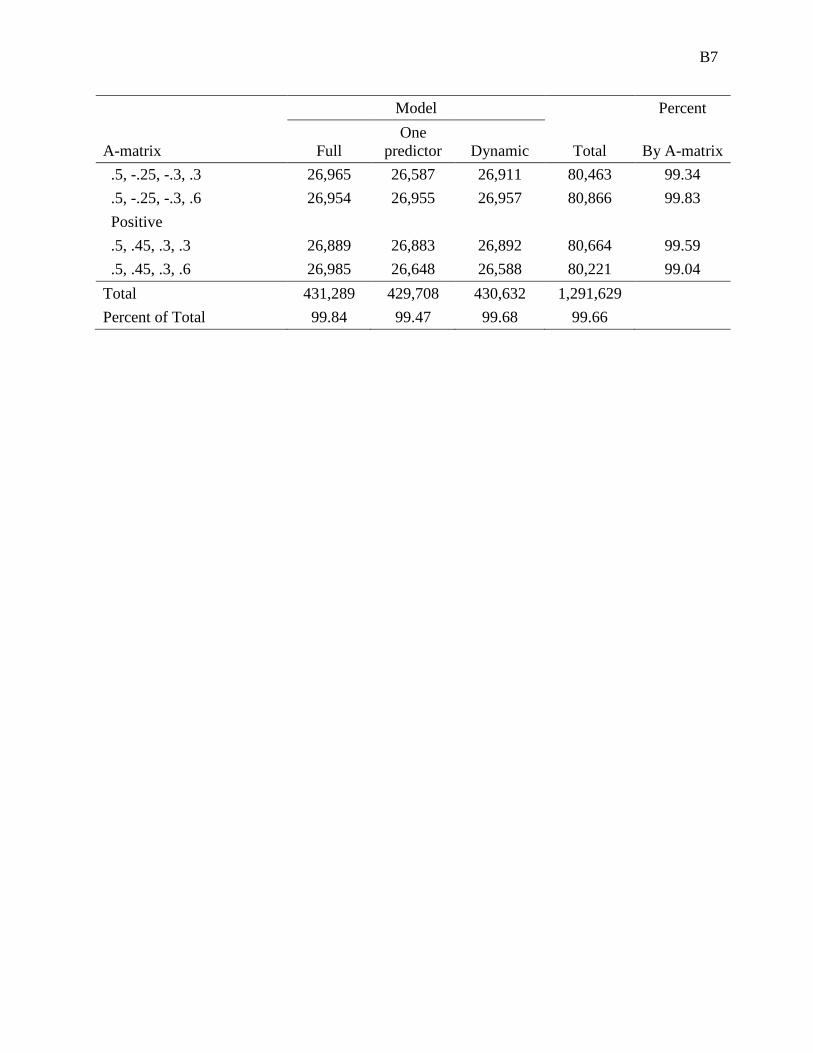
B7

Model Percent

A-matrix Full One

predictor Dynamic Total By A-matrix .5, -.25, -.3, .3 26,965 26,587 26,911 80,463 99.34 .5, -.25, -.3, .6 26,954 26,955 26,957 80,866 99.83 Positive .5, .45, .3, .3 26,889 26,883 26,892 80,664 99.59 .5, .45, .3, .6 26,985 26,648 26,588 80,221 99.04 Total 431,289 429,708 430,632 1,291,629 Percent of Total 99.84 99.47 99.68 99.66

B8

Table B5

Descriptive statistics for all final set of conditions and model estimates without outliers

Mean SD Median Min. Max. Range Skew Kurtosis Full

X 0.07 0.12 0.05 -0.30 0.58 0.88 1.90 5.01 YX 0.02 0.18 0.00 -0.88 0.70 1.57 0.55 4.82 XY 0.05 0.25 0.01 -0.61 1.16 1.78 1.63 5.30 Y 0.15 0.24 0.06 -0.34 1.25 1.59 2.39 5.61 Trait X on TI1 -0.39 0.29 -0.32 -1.92 0.08 2.00 -1.88 4.91 Trait Y on TI1 -0.48 0.30 -0.38 -2.06 -0.12 1.93 -2.00 4.87 One predictor

X 0.09 0.13 0.05 -0.09 0.62 0.71 2.47 5.69 YX 0.04 0.19 0.00 -0.53 0.73 1.26 1.21 4.15 XY 0.07 0.27 0.01 -0.57 1.21 1.78 1.97 5.88 Y 0.17 0.26 0.07 -0.10 1.31 1.41 2.52 5.84 Trait X on TI1 -0.39 0.29 -0.32 -1.86 0.07 1.94 -1.75 4.50 Trait Y on TI1 -0.48 0.30 -0.38 -2.00 0.02 2.02 -1.91 4.68 Dynamic

X 0.10 0.14 0.06 -0.14 0.61 0.75 2.47 5.75 YX 0.05 0.20 0.00 -0.54 0.72 1.26 1.39 4.04 XY 0.08 0.28 0.02 -0.57 1.23 1.80 1.96 5.64 Y 0.18 0.28 0.08 -0.17 1.34 1.51 2.49 5.70

Note: The descriptive statistics were based on data sets that provided auto-effect estimates larger than -4.0.

B9

Table B6

Average bias of X auto-effect estimates by level of the random intercept correlation for full, one predictor, and dynamic models

Full One predictor Dynamic

True value Mean SD Mean SD Mean SD Random intercept r = 0

Balanced

.5, -.45, .3, .3 -0.42 0.04 0.01 0.02 0.02 0.03 0.02 .5, -.45, .3, .6 -0.50 0.03 0.00 0.02 0.02 0.02 0.02 .5, -.25, .3, .3 -0.52 0.04 0.01 0.03 0.01 0.04 0.02 .5, -.25, .3, .6 -0.57 0.05 0.00 0.04 0.01 0.05 0.02 .5, .45, -.3, .3 -0.42 0.06 0.01 0.05 0.01 0.05 0.01 .5, .45, -.3, .6 -0.50 0.05 0.01 0.06 0.00 0.06 0.00 One-way

.5, .0, -.3, .3 -0.69 0.04 0.01 0.05 0.01 0.07 0.01 .5, .0, .3, .3 -0.69 0.03 0.00 0.04 0.00 0.05 0.00 .5, .0, -.3, .6 -0.69 0.04 0.01 0.06 0.01 0.07 0.02 .5, .0, .3, .6 -0.69 0.06 0.00 0.05 0.01 0.06 0.01 Positive

.5, .45, .3, .3 -1.61 0.23 0.07 0.26 0.07 0.26 0.07 .5, .45, .3, .6 -1.01 0.03 0.03 0.02 0.03 0.00 0.04 Negative

.5, -.45, -.3, .3 -1.61 0.31 0.04 0.46 0.03 0.56 0.04 .5, -.45, -.3, .6 -1.01 -0.04 0.02 -0.04 0.02 0.04 0.04 .5, -.25, -.3, .3 -0.98 0.07 0.01 0.09 0.01 0.14 0.02 .5, -.25, -.3, .6 -0.85 0.04 0.01 0.07 0.01 0.10 0.01 Random intercept r = -.1

Balanced

.5, -.45, .3, .3 -0.42 0.04 0.04 0.02 0.03 0.02 0.03 .5, -.45, .3, .6 -0.50 0.03 0.04 0.02 0.03 0.02 0.03 .5, -.25, .3, .3 -0.52 0.06 0.04 0.03 0.02 0.04 0.03 .5, -.25, .3, .6 -0.57 0.06 0.05 0.04 0.03 0.05 0.03 .5, .45, -.3, .3 -0.42 0.03 0.02 0.04 0.01 0.05 0.01 .5, .45, -.3, .6 -0.50 0.03 0.02 0.05 0.01 0.06 0.00

B10

Full One predictor Dynamic

True value Mean SD Mean SD Mean SD One-way

.5, .0, -.3, .3 -0.69 0.03 0.05 0.06 0.02 0.07 0.02 .5, .0, .3, .3 -0.69 0.04 0.03 0.03 0.01 0.04 0.01 .5, .0, -.3, .6 -0.69 0.03 0.06 0.07 0.02 0.07 0.02 .5, .0, .3, .6 -0.69 0.07 0.02 0.06 0.01 0.06 0.02 Positive

.5, .45, .3, .3 -1.61 0.24 0.07 0.26 0.07 0.26 0.07 .5, .45, .3, .6 -1.01 -0.10 0.09 -0.01 0.04 -0.02 0.05 Negative

.5, -.45, -.3, .3 -1.61 0.47 0.03 0.54 0.04 0.56 0.04 .5, -.45, -.3, .6 -1.01 -0.02 0.08 0.03 0.05 0.04 0.06 .5, -.25, -.3, .3 -0.98 0.07 0.06 0.14 0.04 0.15 0.03 .5, -.25, -.3, .6 -0.85 0.05 0.04 0.09 0.02 0.10 0.01 Random intercept r =.1

Balanced

.5, -.45, .3, .3 -0.42 0.04 0.05 0.02 0.03 0.02 0.03 .5, -.45, .3, .6 -0.50 0.02 0.04 0.02 0.03 0.02 0.03 .5, -.25, .3, .3 -0.52 0.05 0.05 0.03 0.02 0.04 0.02 .5, -.25, .3, .6 -0.57 0.05 0.04 0.04 0.03 0.04 0.03 .5, .45, -.3, .3 -0.42 0.04 0.02 0.04 0.01 0.05 0.01 .5, .45, -.3, .6 -0.50 0.04 0.02 0.05 0.01 0.06 0.00 One-way

.5, .0, -.3, .3 -0.69 0.07 0.05 0.07 0.02 0.07 0.01 .5, .0, .3, .3 -0.69 0.06 0.04 0.04 0.01 0.04 0.01 .5, .0, -.3, .6 -0.69 0.09 0.06 0.07 0.02 0.08 0.02 .5, .0, .3, .6 -0.69 0.07 0.02 0.06 0.01 0.06 0.02 Positive

.5, .45, .3, .3 -1.61 0.23 0.10 0.26 0.07 0.26 0.07 .5, .45, .3, .6 -1.01 -0.07 0.08 0.00 0.04 -0.01 0.05 Negative

.5, -.45, -.3, .3 -1.61 0.52 0.04 0.54 0.04 0.56 0.04 .5, -.45, -.3, .6 -1.01 -0.06 0.07 0.02 0.05 0.03 0.06 .5, -.25, -.3, .3 -0.98 0.13 0.05 0.14 0.04 0.15 0.03 .5, -.25, -.3, .6 -0.85 0.10 0.05 0.09 0.02 0.10 0.02

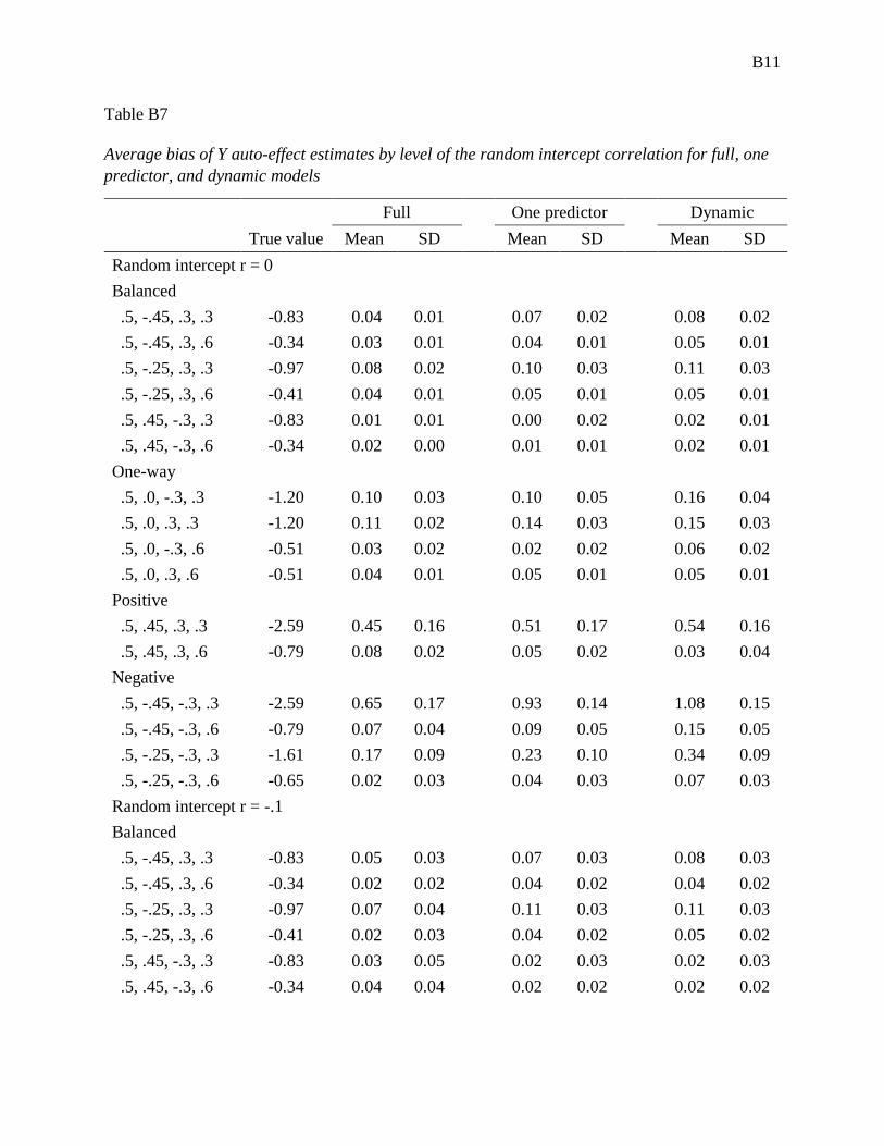
B11

Table B7

Average bias of Y auto-effect estimates by level of the random intercept correlation for full, one predictor, and dynamic models

Full One predictor Dynamic

True value Mean SD Mean SD Mean SD Random intercept r = 0

Balanced

.5, -.45, .3, .3 -0.83 0.04 0.01 0.07 0.02 0.08 0.02 .5, -.45, .3, .6 -0.34 0.03 0.01 0.04 0.01 0.05 0.01 .5, -.25, .3, .3 -0.97 0.08 0.02 0.10 0.03 0.11 0.03 .5, -.25, .3, .6 -0.41 0.04 0.01 0.05 0.01 0.05 0.01 .5, .45, -.3, .3 -0.83 0.01 0.01 0.00 0.02 0.02 0.01 .5, .45, -.3, .6 -0.34 0.02 0.00 0.01 0.01 0.02 0.01 One-way

.5, .0, -.3, .3 -1.20 0.10 0.03 0.10 0.05 0.16 0.04 .5, .0, .3, .3 -1.20 0.11 0.02 0.14 0.03 0.15 0.03 .5, .0, -.3, .6 -0.51 0.03 0.02 0.02 0.02 0.06 0.02 .5, .0, .3, .6 -0.51 0.04 0.01 0.05 0.01 0.05 0.01 Positive

.5, .45, .3, .3 -2.59 0.45 0.16 0.51 0.17 0.54 0.16 .5, .45, .3, .6 -0.79 0.08 0.02 0.05 0.02 0.03 0.04 Negative

.5, -.45, -.3, .3 -2.59 0.65 0.17 0.93 0.14 1.08 0.15 .5, -.45, -.3, .6 -0.79 0.07 0.04 0.09 0.05 0.15 0.05 .5, -.25, -.3, .3 -1.61 0.17 0.09 0.23 0.10 0.34 0.09 .5, -.25, -.3, .6 -0.65 0.02 0.03 0.04 0.03 0.07 0.03 Random intercept r = -.1

Balanced

.5, -.45, .3, .3 -0.83 0.05 0.03 0.07 0.03 0.08 0.03 .5, -.45, .3, .6 -0.34 0.02 0.02 0.04 0.02 0.04 0.02 .5, -.25, .3, .3 -0.97 0.07 0.04 0.11 0.03 0.11 0.03 .5, -.25, .3, .6 -0.41 0.02 0.03 0.04 0.02 0.05 0.02 .5, .45, -.3, .3 -0.83 0.03 0.05 0.02 0.03 0.02 0.03 .5, .45, -.3, .6 -0.34 0.04 0.04 0.02 0.02 0.02 0.02

B12

Full One predictor Dynamic

True value Mean SD Mean SD Mean SD One-way

.5, .0, -.3, .3 -1.20 0.13 0.07 0.14 0.06 0.15 0.06 .5, .0, .3, .3 -1.20 0.11 0.04 0.12 0.04 0.14 0.03 .5, .0, -.3, .6 -0.51 0.04 0.03 0.05 0.02 0.06 0.03 .5, .0, .3, .6 -0.51 0.00 0.06 0.04 0.02 0.05 0.02 Positive

.5, .45, .3, .3 -2.59 0.53 0.17 0.55 0.16 0.54 0.16 .5, .45, .3, .6 -0.79 -0.07 0.11 0.03 0.04 0.01 0.07 Negative

.5, -.45, -.3, .3 -2.59 0.95 0.14 1.06 0.15 1.09 0.14 .5, -.45, -.3, .6 -0.79 0.09 0.10 0.14 0.07 0.15 0.06 .5, -.25, -.3, .3 -1.61 0.24 0.10 0.33 0.09 0.34 0.09 .5, -.25, -.3, .6 -0.65 0.03 0.05 0.06 0.04 0.07 0.03 Random intercept r =.1

Balanced

.5, -.45, .3, .3 -0.83 0.05 0.02 0.07 0.03 0.08 0.02 .5, -.45, .3, .6 -0.34 0.03 0.02 0.04 0.02 0.04 0.02 .5, -.25, .3, .3 -0.97 0.09 0.04 0.11 0.03 0.12 0.03 .5, -.25, .3, .6 -0.41 0.03 0.04 0.04 0.02 0.05 0.02 .5, .45, -.3, .3 -0.83 0.01 0.04 0.02 0.03 0.01 0.03 .5, .45, -.3, .6 -0.34 0.03 0.04 0.02 0.02 0.02 0.02 One-way

.5, .0, -.3, .3 -1.20 0.13 0.09 0.14 0.05 0.15 0.06 .5, .0, .3, .3 -1.20 0.17 0.08 0.14 0.03 0.14 0.03 .5, .0, -.3, .6 -0.51 0.05 0.04 0.05 0.02 0.05 0.03 .5, .0, .3, .6 -0.51 0.04 0.06 0.04 0.02 0.05 0.02 Positive

.5, .45, .3, .3 -2.59 0.56 0.19 0.55 0.15 0.55 0.15 .5, .45, .3, .6 -0.79 -0.02 0.12 0.03 0.05 0.02 0.07 Negative

.5, -.45, -.3, .3 -2.59 1.02 0.12 1.06 0.14 1.09 0.14 .5, -.45, -.3, .6 -0.79 0.23 0.11 0.14 0.06 0.16 0.06 .5, -.25, -.3, .3 -1.61 0.28 0.11 0.33 0.09 0.34 0.09 .5, -.25, -.3, .6 -0.65 0.08 0.05 0.06 0.04 0.07 0.03

B13

Table B8

Average bias of YX cross-effect estimates by level of the random intercept correlation for full, one predictor, and dynamic models

Full One predictor Dynamic

True value Mean SD Mean SD Mean SD Random intercept r = 0

Balanced

.5, -.45, .3, .3 0.61 -0.02 0.00 -0.02 0.01 -0.02 0.01 .5, -.45, .3, .6 0.48 -0.01 0.00 -0.01 0.01 -0.01 0.00 .5, -.25, .3, .3 0.67 -0.02 0.01 -0.02 0.01 -0.01 0.01 .5, -.25, .3, .6 0.51 0.00 0.00 0.00 0.01 0.00 0.00 .5, .45, -.3, .3 -0.61 0.01 0.01 0.02 0.00 0.04 0.01 .5, .45, -.3, .6 -0.48 0.00 0.00 0.00 0.00 0.00 0.00 One-way

.5, .0, -.3, .3 -0.77 0.04 0.01 0.07 0.01 0.11 0.02 .5, .0, .3, .3 0.77 -0.05 0.01 -0.05 0.01 -0.04 0.01 .5, .0, -.3, .6 -0.55 0.02 0.01 0.03 0.01 0.05 0.02 .5, .0, .3, .6 0.55 0.00 0.00 0.00 0.00 0.00 0.00 Positive

.5, .45, .3, .3 1.46 -0.32 0.09 -0.34 0.08 -0.31 0.09 .5, .45, .3, .6 0.66 -0.05 0.01 -0.08 0.01 -0.11 0.04 Negative

.5, -.45, -.3, .3 -1.46 0.36 0.05 0.56 0.04 0.66 0.05 .5, -.45, -.3, .6 -0.66 0.04 0.01 0.05 0.01 0.11 0.03 .5, -.25, -.3, .3 -0.95 0.13 0.02 0.17 0.01 0.23 0.02 .5, -.25, -.3, .6 -0.60 0.07 0.01 0.09 0.01 0.12 0.01 Random intercept r = -.1

Balanced

.5, -.45, .3, .3 0.61 -0.01 0.02 -0.02 0.01 -0.02 0.01 .5, -.45, .3, .6 0.48 0.00 0.01 -0.01 0.01 -0.01 0.01 .5, -.25, .3, .3 0.67 0.00 0.02 -0.01 0.01 -0.01 0.01 .5, -.25, .3, .6 0.51 0.01 0.01 0.00 0.01 0.00 0.01 .5, .45, -.3, .3 -0.61 0.00 0.04 0.02 0.01 0.04 0.01 .5, .45, -.3, .6 -0.48 -0.03 0.03 -0.01 0.01 0.00 0.00

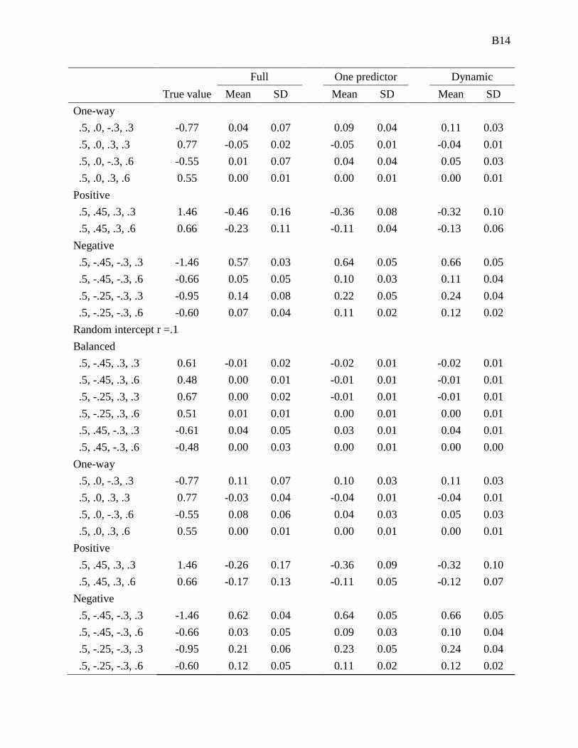
B14

Full One predictor Dynamic

True value Mean SD Mean SD Mean SD One-way

.5, .0, -.3, .3 -0.77 0.04 0.07 0.09 0.04 0.11 0.03 .5, .0, .3, .3 0.77 -0.05 0.02 -0.05 0.01 -0.04 0.01 .5, .0, -.3, .6 -0.55 0.01 0.07 0.04 0.04 0.05 0.03 .5, .0, .3, .6 0.55 0.00 0.01 0.00 0.01 0.00 0.01 Positive

.5, .45, .3, .3 1.46 -0.46 0.16 -0.36 0.08 -0.32 0.10 .5, .45, .3, .6 0.66 -0.23 0.11 -0.11 0.04 -0.13 0.06 Negative

.5, -.45, -.3, .3 -1.46 0.57 0.03 0.64 0.05 0.66 0.05 .5, -.45, -.3, .6 -0.66 0.05 0.05 0.10 0.03 0.11 0.04 .5, -.25, -.3, .3 -0.95 0.14 0.08 0.22 0.05 0.24 0.04 .5, -.25, -.3, .6 -0.60 0.07 0.04 0.11 0.02 0.12 0.02 Random intercept r =.1

Balanced

.5, -.45, .3, .3 0.61 -0.01 0.02 -0.02 0.01 -0.02 0.01 .5, -.45, .3, .6 0.48 0.00 0.01 -0.01 0.01 -0.01 0.01 .5, -.25, .3, .3 0.67 0.00 0.02 -0.01 0.01 -0.01 0.01 .5, -.25, .3, .6 0.51 0.01 0.01 0.00 0.01 0.00 0.01 .5, .45, -.3, .3 -0.61 0.04 0.05 0.03 0.01 0.04 0.01 .5, .45, -.3, .6 -0.48 0.00 0.03 0.00 0.01 0.00 0.00 One-way

.5, .0, -.3, .3 -0.77 0.11 0.07 0.10 0.03 0.11 0.03 .5, .0, .3, .3 0.77 -0.03 0.04 -0.04 0.01 -0.04 0.01 .5, .0, -.3, .6 -0.55 0.08 0.06 0.04 0.03 0.05 0.03 .5, .0, .3, .6 0.55 0.00 0.01 0.00 0.01 0.00 0.01 Positive

.5, .45, .3, .3 1.46 -0.26 0.17 -0.36 0.09 -0.32 0.10 .5, .45, .3, .6 0.66 -0.17 0.13 -0.11 0.05 -0.12 0.07 Negative

.5, -.45, -.3, .3 -1.46 0.62 0.04 0.64 0.05 0.66 0.05 .5, -.45, -.3, .6 -0.66 0.03 0.05 0.09 0.03 0.10 0.04 .5, -.25, -.3, .3 -0.95 0.21 0.06 0.23 0.05 0.24 0.04 .5, -.25, -.3, .6 -0.60 0.12 0.05 0.11 0.02 0.12 0.02

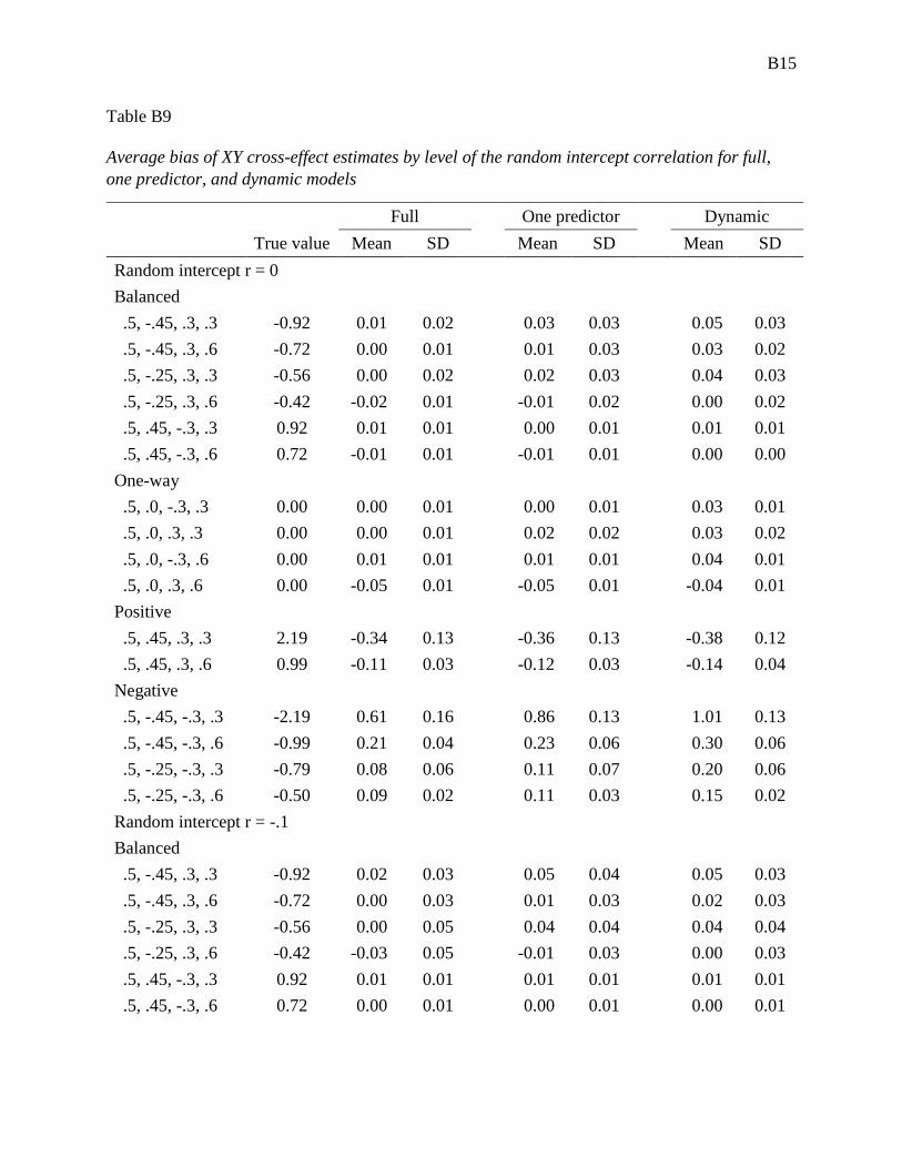
B15

Table B9

Average bias of XY cross-effect estimates by level of the random intercept correlation for full, one predictor, and dynamic models

Full One predictor Dynamic

True value Mean SD Mean SD Mean SD Random intercept r = 0

Balanced

.5, -.45, .3, .3 -0.92 0.01 0.02 0.03 0.03 0.05 0.03 .5, -.45, .3, .6 -0.72 0.00 0.01 0.01 0.03 0.03 0.02 .5, -.25, .3, .3 -0.56 0.00 0.02 0.02 0.03 0.04 0.03 .5, -.25, .3, .6 -0.42 -0.02 0.01 -0.01 0.02 0.00 0.02 .5, .45, -.3, .3 0.92 0.01 0.01 0.00 0.01 0.01 0.01 .5, .45, -.3, .6 0.72 -0.01 0.01 -0.01 0.01 0.00 0.00 One-way

.5, .0, -.3, .3 0.00 0.00 0.01 0.00 0.01 0.03 0.01 .5, .0, .3, .3 0.00 0.00 0.01 0.02 0.02 0.03 0.02 .5, .0, -.3, .6 0.00 0.01 0.01 0.01 0.01 0.04 0.01 .5, .0, .3, .6 0.00 -0.05 0.01 -0.05 0.01 -0.04 0.01 Positive

.5, .45, .3, .3 2.19 -0.34 0.13 -0.36 0.13 -0.38 0.12 .5, .45, .3, .6 0.99 -0.11 0.03 -0.12 0.03 -0.14 0.04 Negative

.5, -.45, -.3, .3 -2.19 0.61 0.16 0.86 0.13 1.01 0.13 .5, -.45, -.3, .6 -0.99 0.21 0.04 0.23 0.06 0.30 0.06 .5, -.25, -.3, .3 -0.79 0.08 0.06 0.11 0.07 0.20 0.06 .5, -.25, -.3, .6 -0.50 0.09 0.02 0.11 0.03 0.15 0.02 Random intercept r = -.1

Balanced

.5, -.45, .3, .3 -0.92 0.02 0.03 0.05 0.04 0.05 0.03 .5, -.45, .3, .6 -0.72 0.00 0.03 0.01 0.03 0.02 0.03 .5, -.25, .3, .3 -0.56 0.00 0.05 0.04 0.04 0.04 0.04 .5, -.25, .3, .6 -0.42 -0.03 0.05 -0.01 0.03 0.00 0.03 .5, .45, -.3, .3 0.92 0.01 0.01 0.01 0.01 0.01 0.01 .5, .45, -.3, .6 0.72 0.00 0.01 0.00 0.01 0.00 0.01

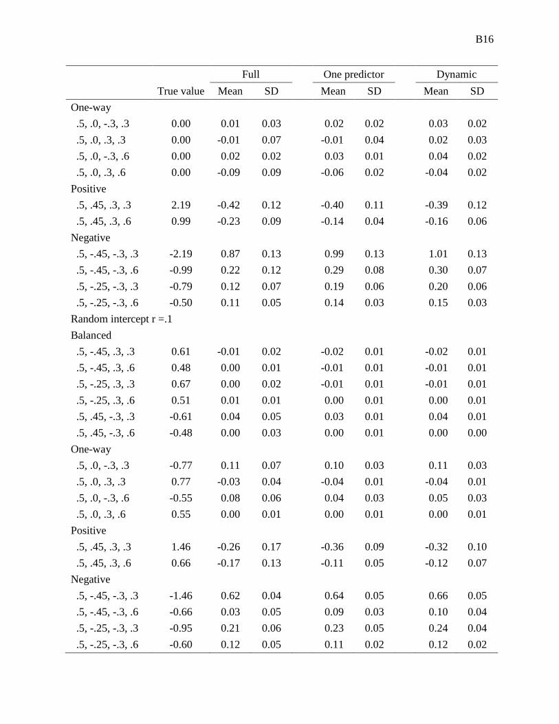
B16

Full One predictor Dynamic

True value Mean SD Mean SD Mean SD One-way

.5, .0, -.3, .3 0.00 0.01 0.03 0.02 0.02 0.03 0.02 .5, .0, .3, .3 0.00 -0.01 0.07 -0.01 0.04 0.02 0.03 .5, .0, -.3, .6 0.00 0.02 0.02 0.03 0.01 0.04 0.02 .5, .0, .3, .6 0.00 -0.09 0.09 -0.06 0.02 -0.04 0.02 Positive

.5, .45, .3, .3 2.19 -0.42 0.12 -0.40 0.11 -0.39 0.12 .5, .45, .3, .6 0.99 -0.23 0.09 -0.14 0.04 -0.16 0.06 Negative

.5, -.45, -.3, .3 -2.19 0.87 0.13 0.99 0.13 1.01 0.13 .5, -.45, -.3, .6 -0.99 0.22 0.12 0.29 0.08 0.30 0.07 .5, -.25, -.3, .3 -0.79 0.12 0.07 0.19 0.06 0.20 0.06 .5, -.25, -.3, .6 -0.50 0.11 0.05 0.14 0.03 0.15 0.03 Random intercept r =.1

Balanced

.5, -.45, .3, .3 0.61 -0.01 0.02 -0.02 0.01 -0.02 0.01 .5, -.45, .3, .6 0.48 0.00 0.01 -0.01 0.01 -0.01 0.01 .5, -.25, .3, .3 0.67 0.00 0.02 -0.01 0.01 -0.01 0.01 .5, -.25, .3, .6 0.51 0.01 0.01 0.00 0.01 0.00 0.01 .5, .45, -.3, .3 -0.61 0.04 0.05 0.03 0.01 0.04 0.01 .5, .45, -.3, .6 -0.48 0.00 0.03 0.00 0.01 0.00 0.00 One-way

.5, .0, -.3, .3 -0.77 0.11 0.07 0.10 0.03 0.11 0.03 .5, .0, .3, .3 0.77 -0.03 0.04 -0.04 0.01 -0.04 0.01 .5, .0, -.3, .6 -0.55 0.08 0.06 0.04 0.03 0.05 0.03 .5, .0, .3, .6 0.55 0.00 0.01 0.00 0.01 0.00 0.01 Positive

.5, .45, .3, .3 1.46 -0.26 0.17 -0.36 0.09 -0.32 0.10 .5, .45, .3, .6 0.66 -0.17 0.13 -0.11 0.05 -0.12 0.07 Negative

.5, -.45, -.3, .3 -1.46 0.62 0.04 0.64 0.05 0.66 0.05 .5, -.45, -.3, .6 -0.66 0.03 0.05 0.09 0.03 0.10 0.04 .5, -.25, -.3, .3 -0.95 0.21 0.06 0.23 0.05 0.24 0.04 .5, -.25, -.3, .6 -0.60 0.12 0.05 0.11 0.02 0.12 0.02

B17

Table B10

Average bias of time-invariant effect on X trait variance by level of the random intercept correlation for full and one predictor

Full One predictor

True value Mean SD Mean SD Random intercept r = 0

Balanced

.5, -.45, .3, .3 0.55 -0.11 0.00 -0.11 0.09 .5, -.45, .3, .6 0.52 -0.12 0.00 -0.12 0.08 .5, -.25, .3, .3 0.50 -0.16 0.01 -0.16 0.08 .5, -.25, .3, .6 0.48 -0.16 0.00 -0.16 0.07 .5, .45, -.3, .3 0.16 -0.37 0.01 -0.37 0.02 .5, .45, -.3, .6 0.23 -0.34 0.00 -0.35 0.03 One-way

.5, .0, -.3, .3 0.42 -0.22 0.00 -0.23 0.06 .5, .0, .3, .3 0.42 -0.22 0.00 -0.22 0.06 .5, .0, -.3, .6 0.42 -0.23 0.01 -0.23 0.06 .5, .0, .3, .6 0.42 -0.21 0.00 -0.20 0.06 Positive

.5, .45, .3, .3 0.06 -0.29 0.03 -0.29 0.03 .5, .45, .3, .6 0.27 -0.28 0.02 -0.28 0.02 Negative

.5, -.45, -.3, .3 1.26 -0.32 0.06 -0.45 0.14 .5, -.45, -.3, .6 0.72 -0.12 0.02 -0.13 0.10 .5, -.25, -.3, .3 0.68 -0.16 0.02 -0.18 0.10 .5, -.25, -.3, .6 0.56 -0.18 0.01 -0.19 0.08 Random intercept r = -.1

Balanced

.5, -.45, .3, .3 -0.92 0.02 0.03 0.05 0.04 .5, -.45, .3, .6 -0.72 0.00 0.03 0.01 0.03 .5, -.25, .3, .3 -0.56 0.00 0.05 0.04 0.04 .5, -.25, .3, .6 -0.42 -0.03 0.05 -0.01 0.03 .5, .45, -.3, .3 0.92 0.01 0.01 0.01 0.01 .5, .45, -.3, .6 0.72 0.00 0.01 0.00 0.01

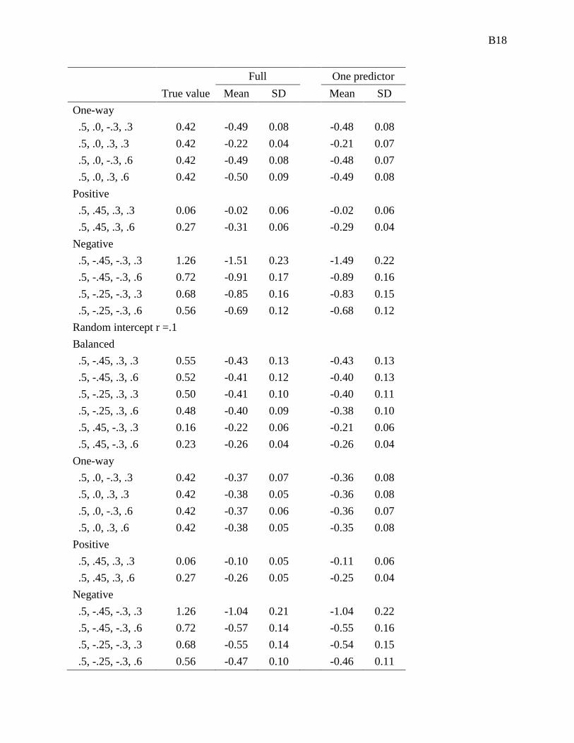
B18

Full One predictor

True value Mean SD Mean SD One-way

.5, .0, -.3, .3 0.42 -0.49 0.08 -0.48 0.08 .5, .0, .3, .3 0.42 -0.22 0.04 -0.21 0.07 .5, .0, -.3, .6 0.42 -0.49 0.08 -0.48 0.07 .5, .0, .3, .6 0.42 -0.50 0.09 -0.49 0.08 Positive

.5, .45, .3, .3 0.06 -0.02 0.06 -0.02 0.06 .5, .45, .3, .6 0.27 -0.31 0.06 -0.29 0.04 Negative

.5, -.45, -.3, .3 1.26 -1.51 0.23 -1.49 0.22 .5, -.45, -.3, .6 0.72 -0.91 0.17 -0.89 0.16 .5, -.25, -.3, .3 0.68 -0.85 0.16 -0.83 0.15 .5, -.25, -.3, .6 0.56 -0.69 0.12 -0.68 0.12 Random intercept r =.1

Balanced

.5, -.45, .3, .3 0.55 -0.43 0.13 -0.43 0.13 .5, -.45, .3, .6 0.52 -0.41 0.12 -0.40 0.13 .5, -.25, .3, .3 0.50 -0.41 0.10 -0.40 0.11 .5, -.25, .3, .6 0.48 -0.40 0.09 -0.38 0.10 .5, .45, -.3, .3 0.16 -0.22 0.06 -0.21 0.06 .5, .45, -.3, .6 0.23 -0.26 0.04 -0.26 0.04 One-way

.5, .0, -.3, .3 0.42 -0.37 0.07 -0.36 0.08 .5, .0, .3, .3 0.42 -0.38 0.05 -0.36 0.08 .5, .0, -.3, .6 0.42 -0.37 0.06 -0.36 0.07 .5, .0, .3, .6 0.42 -0.38 0.05 -0.35 0.08 Positive

.5, .45, .3, .3 0.06 -0.10 0.05 -0.11 0.06 .5, .45, .3, .6 0.27 -0.26 0.05 -0.25 0.04 Negative

.5, -.45, -.3, .3 1.26 -1.04 0.21 -1.04 0.22 .5, -.45, -.3, .6 0.72 -0.57 0.14 -0.55 0.16 .5, -.25, -.3, .3 0.68 -0.55 0.14 -0.54 0.15 .5, -.25, -.3, .6 0.56 -0.47 0.10 -0.46 0.11

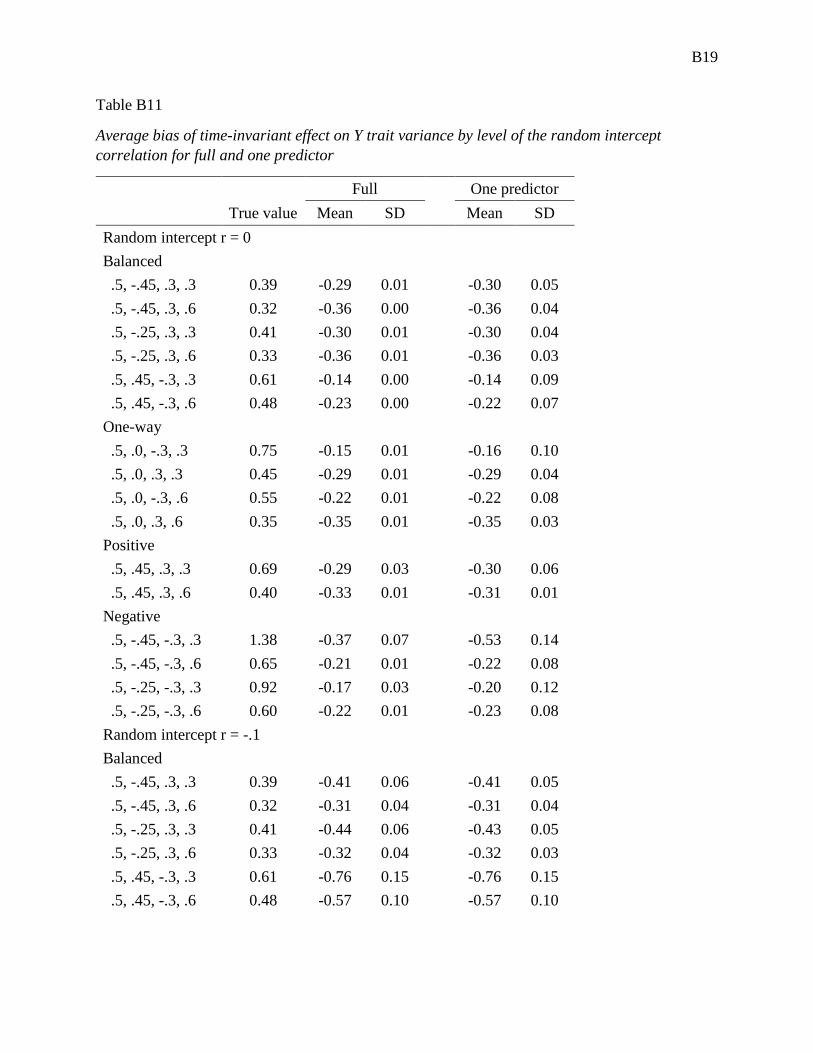
B19

Table B11

Average bias of time-invariant effect on Y trait variance by level of the random intercept correlation for full and one predictor

Full One predictor

True value Mean SD Mean SD Random intercept r = 0

Balanced

.5, -.45, .3, .3 0.39 -0.29 0.01 -0.30 0.05 .5, -.45, .3, .6 0.32 -0.36 0.00 -0.36 0.04 .5, -.25, .3, .3 0.41 -0.30 0.01 -0.30 0.04 .5, -.25, .3, .6 0.33 -0.36 0.01 -0.36 0.03 .5, .45, -.3, .3 0.61 -0.14 0.00 -0.14 0.09 .5, .45, -.3, .6 0.48 -0.23 0.00 -0.22 0.07 One-way

.5, .0, -.3, .3 0.75 -0.15 0.01 -0.16 0.10 .5, .0, .3, .3 0.45 -0.29 0.01 -0.29 0.04 .5, .0, -.3, .6 0.55 -0.22 0.01 -0.22 0.08 .5, .0, .3, .6 0.35 -0.35 0.01 -0.35 0.03 Positive

.5, .45, .3, .3 0.69 -0.29 0.03 -0.30 0.06 .5, .45, .3, .6 0.40 -0.33 0.01 -0.31 0.01 Negative

.5, -.45, -.3, .3 1.38 -0.37 0.07 -0.53 0.14 .5, -.45, -.3, .6 0.65 -0.21 0.01 -0.22 0.08 .5, -.25, -.3, .3 0.92 -0.17 0.03 -0.20 0.12 .5, -.25, -.3, .6 0.60 -0.22 0.01 -0.23 0.08 Random intercept r = -.1

Balanced

.5, -.45, .3, .3 0.39 -0.41 0.06 -0.41 0.05 .5, -.45, .3, .6 0.32 -0.31 0.04 -0.31 0.04 .5, -.25, .3, .3 0.41 -0.44 0.06 -0.43 0.05 .5, -.25, .3, .6 0.33 -0.32 0.04 -0.32 0.03 .5, .45, -.3, .3 0.61 -0.76 0.15 -0.76 0.15 .5, .45, -.3, .6 0.48 -0.57 0.10 -0.57 0.10

B20

Full One predictor

True value Mean SD Mean SD One-way

.5, .0, -.3, .3 0.75 -0.94 0.18 -0.93 0.17 .5, .0, .3, .3 0.45 -0.28 0.02 -0.29 0.05 .5, .0, -.3, .6 0.55 -0.65 0.11 -0.65 0.11 .5, .0, .3, .6 0.35 -0.35 0.04 -0.34 0.03 Positive

.5, .45, .3, .3 0.69 -0.82 0.14 -0.78 0.10 .5, .45, .3, .6 0.40 -0.44 0.07 -0.42 0.04 Negative

.5, -.45, -.3, .3 1.38 -1.64 0.24 -1.62 0.23 .5, -.45, -.3, .6 0.65 -0.79 0.13 -0.78 0.12 .5, -.25, -.3, .3 0.92 -1.15 0.21 -1.13 0.20 .5, -.25, -.3, .6 0.60 -0.72 0.12 -0.71 0.12 Random intercept r =.1

Balanced

.5, -.45, .3, .3 0.39 -0.38 0.05 -0.38 0.05 .5, -.45, .3, .6 0.32 -0.34 0.04 -0.34 0.04 .5, -.25, .3, .3 0.41 -0.40 0.05 -0.39 0.05 .5, -.25, .3, .6 0.33 -0.35 0.03 -0.35 0.04 .5, .45, -.3, .3 0.61 -0.49 0.14 -0.48 0.15 .5, .45, -.3, .6 0.48 -0.42 0.09 -0.41 0.10 One-way

.5, .0, -.3, .3 0.75 -0.60 0.16 -0.59 0.17 .5, .0, .3, .3 0.45 -0.44 0.04 -0.42 0.06 .5, .0, -.3, .6 0.55 -0.47 0.09 -0.45 0.11 .5, .0, .3, .6 0.35 -0.37 0.02 -0.36 0.03 Positive

.5, .45, .3, .3 0.69 -0.64 0.08 -0.61 0.10 .5, .45, .3, .6 0.40 -0.38 0.05 -0.37 0.04 Negative

.5, -.45, -.3, .3 1.38 -1.16 0.22 -1.15 0.22 .5, -.45, -.3, .6 0.65 -0.55 0.10 -0.54 0.12 .5, -.25, -.3, .3 0.92 -0.73 0.19 -0.73 0.20 .5, -.25, -.3, .6 0.60 -0.51 0.10 -0.49 0.11

B21

Table B12

X auto-effect relative bias for comparison of full to omitted variable models averaged over A-matrix simulation conditions

Full / One Predictor

Full / Dynamic

With Outliers

Without Outliers

With

Outliers Without Outliers

Balanced

.5, -.45, .3, .3 2.22 2.22 2.55 2.48 .5, -.45, .3, .6 2.06 2.05 -0.47 -0.46 .5, -.25, .3, .3 1.84 1.79 1.80 1.42 .5, -.25, .3, .6 1.41 1.43 1.25 1.25 .5, .45, -.3, .3 0.91 0.91 0.89 0.89 .5, .45, -.3, .6 0.71 0.71 0.70 0.70 One-way

.5, .0, -.3, .3 0.79 0.79 0.66 0.66 .5, .0, .3, .3 1.18 1.20 0.92 0.96 .5, .0, -.3, .6 0.85 0.85 0.75 0.75 .5, .0, .3, .6 1.23 1.23 1.11 1.13 Positive

.5, .45, .3, .3 0.86 0.88 0.86 0.88 .5, .45, .3, .6 1.21 1.84 -0.32 -0.33 Negative

.5, -.45, -.3, .3 0.38 0.84 0.32 0.79 .5, -.45, -.3, .6 1.49 1.31 1.18 0.27 .5, -.25, -.3, .3 0.57 0.75 0.51 0.62 .5, -.25, -.3, .6 0.77 0.81 0.68 0.69

Note. Relative bias greater than 1 indicates that the omitted model was less biased than the full model. Relative bias less than 1 indicates that the full model was less biased than the omitted variable model.

B22

Table B13

Y auto-effect relative bias for comparison of full to omitted variable models averaged over A-matrix simulation conditions

Full / One Predictor

Full / Dynamic

With Outliers

Without Outliers

With

Outliers Without Outliers

Balanced

.5, -.45, .3, .3 0.71 0.71 0.67 0.67 .5, -.45, .3, .6 0.22 0.25 0.61 0.46 .5, -.25, .3, .3 0.73 0.76 0.72 0.72 .5, -.25, .3, .6 0.77 0.79 0.85 0.81 .5, .45, -.3, .3 0.61 0.61 0.65 0.65 .5, .45, -.3, .6 0.59 0.59 0.44 0.66 One-way

.5, .0, -.3, .3 1.07 1.07 0.83 0.83 .5, .0, .3, .3 1.02 1.03 0.91 0.93 .5, .0, -.3, .6 1.20 1.20 0.84 0.84 .5, .0, .3, .6 0.67 0.67 0.56 0.57 Positive

.5, .45, .3, .3 0.97 0.96 0.91 0.94 .5, .45, .3, .6 -0.11 -0.10 0.25 0.26 Negative

.5, -.45, -.3, .3 0.39 0.85 0.46 0.81 .5, -.45, -.3, .6 0.47 1.13 -0.68 0.88 .5, -.25, -.3, .3 0.75 0.78 0.42 0.66 .5, -.25, -.3, .6 0.97 1.01 0.77 0.77

Note. Relative bias greater than 1 indicates that the omitted model was less biased than the full model. Relative bias less than 1 indicates that the full model was less biased than the omitted variable model.

B23

Table B14

YX cross-effect relative bias for comparison of full to omitted variable models averaged over A-matrix simulation conditions

Full / One Predictor

Full / Dynamic

With Outliers

Without Outliers

With

Outliers Without Outliers

Balanced

.5, -.45, .3, .3 0.41 0.41 0.52 0.53 .5, -.45, .3, .6 0.98 0.40 4.54 4.59 .5, -.25, .3, .3 0.04 0.06 -3.44 -3.33 .5, -.25, .3, .6 14.42 14.60 0.73 -0.34 .5, .45, -.3, .3 0.74 0.74 0.49 0.49 .5, .45, -.3, .6 2.32 2.32 17.35 17.29 One-way

.5, .0, -.3, .3 0.83 0.83 0.66 0.66 .5, .0, .3, .3 0.85 0.88 1.00 1.04 .5, .0, -.3, .6 0.68 0.68 4.44 4.45 .5, .0, .3, .6 -2.23 -2.21 -33.80 -33.76 Positive

.5, .45, .3, .3 0.96 0.97 1.20 1.15 .5, .45, .3, .6 1.43 1.43 1.30 1.30 Negative

.5, -.45, -.3, .3 0.30 0.84 19.99 0.79 .5, -.45, -.3, .6 0.07 0.44 0.17 0.24 .5, -.25, -.3, .3 2.13 0.80 0.97 0.70 .5, -.25, -.3, .6 0.82 0.87 0.75 0.76

Note. Relative bias greater than 1 indicates that the omitted model was less biased than the full model. Relative bias less than 1 indicates that the full model was less biased than the omitted variable model.

B24

Table B15

XY cross-effect relative bias for comparison of full to omitted variable models averaged over A-matrix simulation conditions

Full / One Predictor

Full / Dynamic

With Outliers

Without Outliers

With

Outliers Without Outliers

Balanced

.5, -.45, .3, .3 1.05 1.05 0.48 0.47 .5, -.45, .3, .6 2.30 2.47 1.61 1.64 .5, -.25, .3, .3 0.97 1.05 0.95 0.85 .5, -.25, .3, .6 0.64 0.70 0.00 0.03 .5, .45, -.3, .3 1.07 1.07 3.90 3.90 .5, .45, -.3, .6 -10.01 -10.01 -8.50 -8.90 One-way

.5, .0, -.3, .3 -0.66 -0.66 -0.19 -0.19 .5, .0, .3, .3 -0.78 -0.78 0.13 0.12 .5, .0, -.3, .6 1.07 1.07 0.75 0.73 .5, .0, .3, .6 0.61 0.61 0.38 0.32 Positive

.5, .45, .3, .3 1.05 1.00 0.98 1.00 .5, .45, .3, .6 1.35 1.35 1.25 1.25 Negative

.5, -.45, -.3, .3 0.40 0.85 0.49 0.80 .5, -.45, -.3, .6 -4.64 1.02 -0.15 0.91 .5, -.25, -.3, .3 -0.58 0.71 0.78 0.57 .5, -.25, -.3, .6 0.82 0.91 0.88 0.82

Note. Relative bias greater than 1 indicates that the omitted model was less biased than the full model. Relative bias less than 1 indicates that the full model was less biased than the omitted variable model.

B25

Table B16

Time-invariant effect relative bias for comparison of full to one predictor model averaged over A-matrix simulation conditions

With Outliers Without Outliers A-matrices TI on X TI on Y TI on X TI on Y Balanced .5, -.45, .3, .3 0.97 1.00 0.97 1.00 .5, -.45, .3, .6 0.46 1.01 0.43 1.01 .5, -.25, .3, .3 1.18 1.01 1.18 1.01 .5, -.25, .3, .6 1.15 1.01 1.15 1.01 .5, .45, -.3, .3 1.02 3.99 1.02 3.99 .5, .45, -.3, .6 1.00 1.06 1.00 1.06 One-way

.5, .0, -.3, .3 1.04 0.03 1.04 0.03 .5, .0, .3, .3 1.10 1.01 1.10 1.02 .5, .0, -.3, .6 1.03 1.07 1.03 1.07 .5, .0, .3, .6 1.07 1.02 1.07 1.02 Positive

.5, .45, .3, .3 0.98 1.04 0.98 1.02 .5, .45, .3, .6 1.03 1.04 1.03 1.04 Negative

.5, -.45, -.3, .3 0.64 0.61 0.93 0.92 .5, -.45, -.3, .6 -0.52 0.77 0.72 1.07 .5, -.25, -.3, .3 0.80 0.63 0.06 1.02 .5, -.25, -.3, .6 1.00 1.31 1.07 1.05

Note. Relative bias greater than 1 indicates that the omitted model was less biased than the full model. Relative bias less than 1 indicates that the full model was less biased than the omitted variable model.

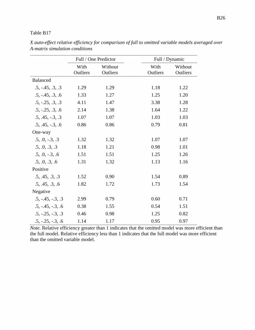
B26

Table B17

X auto-effect relative efficiency for comparison of full to omitted variable models averaged over A-matrix simulation conditions

Full / One Predictor

Full / Dynamic

With Outliers

Without Outliers

With

Outliers Without Outliers

Balanced

.5, -.45, .3, .3 1.29 1.29 1.18 1.22 .5, -.45, .3, .6 1.33 1.27 1.25 1.20 .5, -.25, .3, .3 4.11 1.47 3.38 1.28 .5, -.25, .3, .6 2.14 1.38 1.64 1.22 .5, .45, -.3, .3 1.07 1.07 1.03 1.03 .5, .45, -.3, .6 0.86 0.86 0.79 0.81 One-way

.5, .0, -.3, .3 1.32 1.32 1.07 1.07 .5, .0, .3, .3 1.18 1.21 0.98 1.01 .5, .0, -.3, .6 1.51 1.51 1.25 1.26 .5, .0, .3, .6 1.31 1.32 1.13 1.16 Positive

.5, .45, .3, .3 1.52 0.90 1.54 0.89 .5, .45, .3, .6 1.82 1.72 1.73 1.54 Negative

.5, -.45, -.3, .3 2.99 0.79 0.60 0.71 .5, -.45, -.3, .6 0.38 1.55 0.54 1.51 .5, -.25, -.3, .3 0.46 0.98 1.25 0.82 .5, -.25, -.3, .6 1.14 1.17 0.95 0.97

Note. Relative efficiency greater than 1 indicates that the omitted model was more efficient than the full model. Relative efficiency less than 1 indicates that the full model was more efficient than the omitted variable model.

B27

Table B18

Y auto-effect relative efficiency for comparison of full to omitted variable models averaged over A-matrix simulation conditions

Full / One Predictor

Full / Dynamic

With Outliers

Without Outliers

With

Outliers Without Outliers

Balanced

.5, -.45, .3, .3 0.78 0.78 0.73 0.74 .5, -.45, .3, .6 1.05 0.96 0.89 0.84 .5, -.25, .3, .3 1.37 0.85 1.29 0.79 .5, -.25, .3, .6 1.65 1.16 1.44 0.98 .5, .45, -.3, .3 1.16 1.17 1.19 1.19 .5, .45, -.3, .6 1.66 1.66 1.47 1.51 One-way

.5, .0, -.3, .3 0.99 0.99 0.86 0.86 .5, .0, .3, .3 1.14 1.17 0.99 1.01 .5, .0, -.3, .6 1.13 1.13 0.88 0.89 .5, .0, .3, .6 1.53 1.54 1.15 1.17 Positive

.5, .45, .3, .3 1.31 1.00 1.32 0.98 .5, .45, .3, .6 1.92 1.74 1.83 1.59 Negative

.5, -.45, -.3, .3 1.29 0.78 0.60 0.72 .5, -.45, -.3, .6 0.33 1.76 0.48 1.45 .5, -.25, -.3, .3 0.39 0.82 0.77 0.69 .5, -.25, -.3, .6 1.40 1.43 1.20 1.22

B28

Table B19

YX cross-effect relative efficiency for comparison of full to omitted variable models averaged over A-matrix simulation conditions

Full / One Predictor

Full / Dynamic

With Outliers

Without Outliers

With

Outliers Without Outliers

Balanced

.5, -.45, .3, .3 0.98 0.98 0.98 1.01 .5, -.45, .3, .6 5.58 1.05 6.33 1.08 .5, -.25, .3, .3 26.55 1.09 28.14 1.07 .5, -.25, .3, .6 31.32 1.06 32.42 1.03 .5, .45, -.3, .3 1.57 1.57 1.24 1.24 .5, .45, -.3, .6 1.49 1.49 1.41 1.46 One-way

.5, .0, -.3, .3 1.39 1.39 1.11 1.11 .5, .0, .3, .3 0.96 0.99 1.01 1.04 .5, .0, -.3, .6 2.03 2.03 1.73 1.73 .5, .0, .3, .6 1.09 1.10 1.05 1.07 Positive

.5, .45, .3, .3 1.52 1.07 1.67 1.21 .5, .45, .3, .6 2.03 1.99 1.86 1.77 Negative

.5, -.45, -.3, .3 2.65 0.79 0.59 0.72 .5, -.45, -.3, .6 0.30 1.02 0.43 0.92 .5, -.25, -.3, .3 0.39 0.91 0.80 0.78 .5, -.25, -.3, .6 1.05 1.08 0.91 0.93

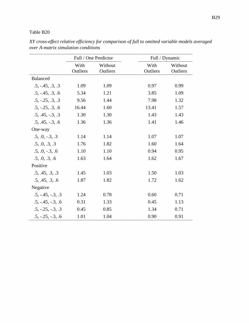
B29

Table B20

XY cross-effect relative efficiency for comparison of full to omitted variable models averaged over A-matrix simulation conditions

Full / One Predictor

Full / Dynamic

With Outliers

Without Outliers

With

Outliers Without Outliers

Balanced

.5, -.45, .3, .3 1.09 1.09 0.97 0.99 .5, -.45, .3, .6 5.34 1.21 3.85 1.09 .5, -.25, .3, .3 9.56 1.44 7.98 1.32 .5, -.25, .3, .6 16.44 1.60 13.41 1.57 .5, .45, -.3, .3 1.30 1.30 1.43 1.43 .5, .45, -.3, .6 1.36 1.36 1.41 1.46 One-way

.5, .0, -.3, .3 1.14 1.14 1.07 1.07 .5, .0, .3, .3 1.76 1.82 1.60 1.64 .5, .0, -.3, .6 1.10 1.10 0.94 0.95 .5, .0, .3, .6 1.63 1.64 1.62 1.67 Positive

.5, .45, .3, .3 1.45 1.03 1.50 1.03 .5, .45, .3, .6 1.87 1.82 1.72 1.62 Negative

.5, -.45, -.3, .3 1.24 0.78 0.60 0.71 .5, -.45, -.3, .6 0.31 1.33 0.45 1.13 .5, -.25, -.3, .3 0.45 0.85 1.34 0.71 .5, -.25, -.3, .6 1.01 1.04 0.90 0.91

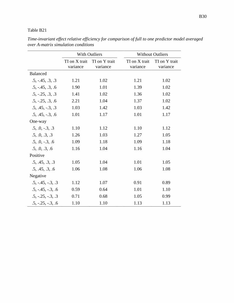
B30

Table B21

Time-invariant effect relative efficiency for comparison of full to one predictor model averaged over A-matrix simulation conditions

With Outliers

Without Outliers

TI on X trait variance

TI on Y trait variance

TI on X trait

variance TI on Y trait

variance Balanced

.5, -.45, .3, .3 1.21 1.02 1.21 1.02 .5, -.45, .3, .6 1.90 1.01 1.39 1.02 .5, -.25, .3, .3 1.41 1.02 1.36 1.02 .5, -.25, .3, .6 2.21 1.04 1.37 1.02 .5, .45, -.3, .3 1.03 1.42 1.03 1.42 .5, .45, -.3, .6 1.01 1.17 1.01 1.17 One-way

.5, .0, -.3, .3 1.10 1.12 1.10 1.12 .5, .0, .3, .3 1.26 1.03 1.27 1.05 .5, .0, -.3, .6 1.09 1.18 1.09 1.18 .5, .0, .3, .6 1.16 1.04 1.16 1.04 Positive

.5, .45, .3, .3 1.05 1.04 1.01 1.05 .5, .45, .3, .6 1.06 1.08 1.06 1.08 Negative

.5, -.45, -.3, .3 1.12 1.07 0.91 0.89 .5, -.45, -.3, .6 0.59 0.64 1.01 1.10 .5, -.25, -.3, .3 0.71 0.68 1.05 0.99 .5, -.25, -.3, .6 1.10 1.10 1.13 1.13