The role of GHG emissions from infrastructure construction ... · PDF fileThe role of GHG...
140
EU Transport GHG: Routes to 2050 II The role of GHG emissions from infrastructure construction, Contract 070307/2010/579469/SER/C2 vehicle manufacturing, and ELVs in overall transport emissions Restricted-Commercial Ref. AEA/ED56293/Task 2 Paper Draft – Issue No. 1 i The role of GHG emissions from infrastructure construction, vehicle manufacturing, and ELVs in overall transport sector emissions Nikolas Hill (AEA) Charlotte Brannigan (AEA) David Wynn (AEA) Robert Milnes (AEA) Huib van Essen (CE Delft) Eelco den Boer (CE Delft) Anouk van Grinsven (CE Delft) Tom Ligthart (TNO) René van Gijlswijk (TNO) 21st April 2011 Draft – Work in Progress
Transcript of The role of GHG emissions from infrastructure construction ... · PDF fileThe role of GHG...
EU Transport GHG: Routes to 2050 II The role of GHG emissions from infrastructure construction, Contract 070307/2010/579469/SER/C2 vehicle manufacturing, and ELVs in overall transport emissions
Restricted-Commercial Ref. AEA/ED56293/Task 2 Paper Draft – Issue No. 1 i
The role of GHG emissions from infrastructure construction, vehicle manufacturing, and ELVs in overall transport sector emissions
Nikolas Hill (AEA) Charlotte Brannigan (AEA) David Wynn (AEA) Robert Milnes (AEA)
Huib van Essen (CE Delft) Eelco den Boer (CE Delft) Anouk van Grinsven (CE Delft)
Tom Ligthart (TNO) René van Gijlswijk (TNO)
21st April 2011 Draft – Work in Progress

The role of GHG emissions from infrastructure construction, EU Transport GHG: Routes to 2050 II vehicle manufacturing, and ELVs in overall transport emissions Contract 070307/2010/579469/SER/C2
Restricted-Commercial Ref. AEA/ED56293/Task 2 Paper Draft – Issue No. 1 ii
Nikolas Hill (AEA) Charlotte Brannigan (AEA) David Wynn (AEA) Robert Milnes (AEA) Huib van Essen (CE Delft) Eelco den Boer (CE Delft) Anouk van Grinsven (CE Delft) Tom Ligthart (TNO) René van Gijlswijk (TNO)
The role of GHG emissions from infrastructure construction, vehicle manufacturing, and ELVs in overall transport sector emissions
21st April 2011 Draft – WIP
Suggested citation: Hill, N. et al (2011) The role of GHG emissions from infrastructure construction, vehicle manufacturing, and ELVs in overall transport sector emissions. Task 2 paper produced as part of a contract between European Commission Directorate-General Climate Action and AEA Technology plc; see website www.eutransportghg2050.eu

EU Transport GHG: Routes to 2050 II The role of GHG emissions from infrastructure construction, Contract 070307/2010/579469/SER/C2 vehicle manufacturing, and ELVs in overall transport emissions
Restricted-Commercial Ref. AEA/ED56293/Task 2 Paper Draft – Issue No. 1 iii
Executive Summary
Introduction
To be completed for Final version


EU Transport GHG: Routes to 2050 II The role of GHG emissions from infrastructure construction, Contract 070307/2010/579469/SER/C2 vehicle manufacturing, and ELVs in overall transport emissions
Restricted-Commercial Ref. AEA/ED56293/Task 2 Paper Draft – Issue No. 1 v
Table of Contents
Executive Summary ................................................................................................ iii
1 Introduction ...................................................................................................... 1
1.1 Topic of this paper .............................................................................................. 1
1.2 The contribution of transport to GHG emissions ................................................. 1
1.3 Background to the project and its objectives ...................................................... 4
1.4 Background and purpose of the paper ............................................................... 6
1.5 Structure of the paper ........................................................................................ 6
2 General Information ......................................................................................... 7
2.1 General emission factors for energy use ............................................................ 7
2.2 General emission factors for raw material production and for material recycling /
other disposal ............................................................................................................... 8
2.3 References........................................................................................................14
3 Infrastructure .................................................................................................. 15
3.1 Road Transport .................................................................................................15
3.2 Rail ...................................................................................................................23
3.3 Aviation .............................................................................................................44
3.4 Shipping ............................................................................................................53
3.5 Energy Carriers .................................................................................................62
4 Vehicle Manufacturing ................................................................................... 73
4.1 Road Transport .................................................................................................73
4.2 Rail ...................................................................................................................93
4.3 Aviation .............................................................................................................97
4.4 Shipping .......................................................................................................... 108
5 Vehicle Disposal ........................................................................................... 114
5.1 Road Transport ............................................................................................... 114
5.2 Rail ................................................................................................................. 118
5.3 Aviation ........................................................................................................... 119
5.4 Shipping .......................................................................................................... 123
6 Reaching Optimal Solutions ....................................................................... 125
6.1 Modal comparisons ......................................................................................... 125
6.2 Comparison of alternate scenarios .................................................................. 125
7 Summary of Key Findings and Conclusions ............................................. 126

EU Transport GHG: Routes to 2050 II The role of GHG emissions from infrastructure construction, Contract 070307/2010/579469/SER/C2 vehicle manufacturing, and ELVs in overall transport emissions
Restricted-Commercial Ref. AEA/ED56293/Task 2 Paper Draft – Issue No. 1 vi
List of Tables
Tables in the main body of the report
Table 2.1: Fuel GHG emission factors defined in SULTAN (kgCO2e/kWh) ........................ 7 Table 2.2: General GHG emission factors for materials used in road vehicles, trains,
aircraft and ships .............................................................................................. 9 Table 2.3: General GHG emission factors for materials used in the construction and
maintenance of transport infrastructure ............................................................10 Table 2.4: Estimates of GHG intensity NiMH and Li-ion batteries based on sources from
the literature .....................................................................................................13 Table 3.1: Current emission factors for road infrastructure. ..............................................20 Table 3.2: Emission reduction potential for measures in road infrastructure. ....................21 Table 3.3: Emissions of CO2 from rail lifecycle scenarios (UIC, 2009) ..............................31 Table 3.4: Rail infrastructure life cycle emissions ..............................................................33 Table 3.5: Emissions for rail infrastructure (kg CO2) .........................................................34 Table 3.6: Rail infrastructure embedded emissions from components and materials ........39 Table 3.7: Rail infrastructure construction energy consumption ........................................40 Table 3.8: Rail infrastructure construction emissions ........................................................40 Table 3.9: Rail infrastructure maintenance energy consumption .......................................41 Table 3.10: Rail infrastructure energy consumption from in use phase ...............................41 Table 3.11: Rail infrastructure emissions from in use phase ...............................................42 Table 3.12 EU Number of Airport by number of passengers carried per year (2010) (EU,
2010) ...............................................................................................................45 Table 3.13: Top Intra-EU country pairs by passengers carried in 2009 (Eurostat, 2011b) ..45 Table 3.14: Top airports in the EU-27 in terms of total passengers carried in 2009 (Eurostat,
2011c) ..............................................................................................................45 Table 3.15: Top airports in the EU-27 in terms of total freight and mail carried in 2009
(Eurostat, 2011c) .............................................................................................46 Table 3.16 : Energy Usage for Aviation Infrastructure Components (ranges of the
parameters are given based on different aircraft sizes) (Adapted from Chester and Horvarth, 2009; 2007) ...............................................................................47
Table 3.17: Key GHG equivalent emissions from Aviation Infrastructure Components (ranges of the parameters are given based on different aircraft sizes) (adapted from Chester and Horvarth, 2009; 2007) ..........................................................47
Table 3.18 Average Energy Consumption and Costs for GSE (adapted from ATAA, 1994; FFA and EPA, 1995; ) ......................................................................................49
Table 3.19: Life-cycle emissions in aviation (Simonsen, 2011) ...........................................51 Table 3.20: Life cycle CO2 emissions of selected ports .......................................................59 Table 3.21: GHG emission intensity of key pipeline raw materials ......................................64 Table 3.22: Total CO2 emissions from laying 1km of steel pipeline (Nacap, 2010) ..............65 Table 3.23: Calculated average length of electricity, natural gas and hydrogen transmission
and distribution networks per customer (Castello et al, 2005) ..........................66 Table 3.24: Methods for Recharging (SWELTRAC12, Vande Bosshe et al; in Nemry and
Bron, 2010) ......................................................................................................68 Table 4.1: Normalised reference values used in this study ...............................................73 Table 4.2: Overview of GHG emissions of passenger car production ...............................74 Table 4.3: Absolute and relative emissions of the vehicle production stage assuming an
average vehicle lifetime of 180, 000 km (g CO2 e./km) .....................................78 Table 4.4: Fuel consumption reducing technologies with the best cost/benefit ratio for
average cars (TNO, 2010) ...............................................................................79

EU Transport GHG: Routes to 2050 II The role of GHG emissions from infrastructure construction, Contract 070307/2010/579469/SER/C2 vehicle manufacturing, and ELVs in overall transport emissions
Restricted-Commercial Ref. AEA/ED56293/Task 2 Paper Draft – Issue No. 1 vii
Table 4.5 Evolution of the composition of cars from 1965-1995 (Smidt and Leithner, 1995) ........................................................................................................................80
Table 4.6: Relative change materials used .......................................................................81 Table 4.7: Material use in case of 30% weight reduction ..................................................81 Table 4.8: Fuel and Electricity consumption values used in LCA (reproduced from Table 2
of Helms et al, 2010) ........................................................................................83 Table 4.9 Vehicle performance of different trucks (adapted from Spielmann et al, 2007) .88 Table 4.10: Comparison of typical current and future conventional (intercity) and high-speed
rail rolling stock ................................................................................................96 Table 4.11: Weight distribution of domestic and international aircrafts. Assumptions from
Probe database (tonnes) (Simonsen, 2011) ................................................... 105 Table 4.12: Emissions to air during production and transportation of materials to Airbus 320,
Airbus A340-600, Boeing 737-300 and Embraer 145 (Simonsen, 2011) ........ 106 Table 4.13: Energy consumption in the production and transportation of materials to Airbus
320, Airbus A340-600, Boeing 737-300 and Embraer 145 (Simonsen, 2011) 106 Table 4.14: Energy & GHG emissions from aircraft and aircraft engine manufacturing
(Simonsen, 2011) .......................................................................................... 108 Table 4.15: Assumptions used in the estimation of lifecycle emissions from shipping ....... 109 Table 4.16: Lifecycle CO2 emissions for ships (adapted from Simonsen, 2010) ................ 110 Table 5.1: Share of use of virgin and recycled material................................................... 116 Table 5.2: Estimated Recycling rates for different materials for the period 2006-2030 .... 116

EU Transport GHG: Routes to 2050 II The role of GHG emissions from infrastructure construction, Contract 070307/2010/579469/SER/C2 vehicle manufacturing, and ELVs in overall transport emissions
Restricted-Commercial Ref. AEA/ED56293/Task 2 Paper Draft – Issue No. 1 viii
List of Figures
Figures in the main body of the report
Figure 1.1: EU27 greenhouse gas emissions by sector and mode of transport, 2007 ....... 1 Figure 1.2: Business as usual projected growth in transport‟s GHG emissions by mode .. 3 Figure 1.3: EU overall emissions trajectories against transport emissions (indexed) ........ 4 Figure 2.1: Assumed low GHG pathway emission factors for selected materials .............12 Figure 3.1 GHG emissions during 40 years of service life of a 13 m wide road in Sweden
(adapted from Stripple, 2001). .......................................................................16 Figure 3.2 GHG emissions from road surface construction and maintenance for different
road surface materials. Congestion includes all construction and maintenance related traffic congestion. Usage includes overlay roughness effects on vehicular travel and fuel consumption during normal traffic flow (after Zhang et al (2008)). ......................................................................................................17
Figure 3.3 Image of artificial light at night time in Europe (NASA). ..................................18 Figure 3.4 Impact on lighting scheme on electricity use related GHG emissions. Option 1
is „blanket lighting‟; option 2A lighting only meets British standards (Fox (2007). ...........................................................................................................20
Figure 3.5: Life-cycle analysis of rail as a whole ..............................................................26 Figure 3.6: Life-cycle analysis of rail infrastructure ..........................................................26 Figure 3.7: Schalupitz assumptions for cross-regional high speed track ..........................27 Figure3.8: Material requirements for various station types ..............................................27 Figure 3.9: Material requirements for various station types ..............................................28 Figure 3.10: Emissions from rail construction by supporting structure, split by component 29 Figure 3.11: Material breakdown for conventional ballasted track ......................................30 Figure 3.12: Material breakdown for ballastless track ........................................................30 Figure 3.13: Breakdown of embedded greenhouse gas emissions of conventional ballasted
track, for production and disposal based on 50% recycling rate .....................30 Figure 3.14: Breakdown of embedded greenhouse gas emissions for ballastless track, for
production and disposal based on 50% recycling rate ...................................30 Figure 3.15: Carbon footprint of High-Speed Rail – CO2 emissions for three scenarios
(adapted from UIC, 2009) ..............................................................................32 Figure 3.16: Carbon footprint of High-Speed Rail – % of CO2 emissions for track system,
rolling stock and operation for three scenarios (adapted from UIC, 2009) ......32 Figure 3.17: Total CO2 emissions for rail infrastructire (kg CO2) (adapted from Claro, 2010)
33 Figure 3.18: Total CO2 emissions for rail infrastructure (%) (Adapted from Claro, 2010) ....34 Figure 3.19: Overview of greenhouse gas emissions from rail infrastructure .....................36 Figure 3.20: Greenhouse gas emissions from rail infrastructure civil engineering works ....36 Figure 3.21: Rail infrastructure construction phase: Ademe, RFF, SNCF (2009) data .......37 Figure 3.22: MAGLEV construction, maintenance and repair CO2 emissions ....................38 Figure 3.23: Comparison of lifecycle emissions for Osaka – Tokyo route, Kato et al (2005)
......................................................................................................................38 Figure 3.24: Life-cycle emissions in aviation (Simonsen, 2011) .........................................51 Figure 3.25: Overview carbon footprint quay walls investigated (Luijten et al, 2010)..........55 Figure 3.26: Carbon footprint for Antarticaweg quay wall in more detail (Luijten et al, 2010)
55 Figure 3.27: CO2 emissions for 1m of quay wall (Maas, 2011)...........................................56 Figure 3.28: CO2 emissions for 1m of quay retaining wall (Maas, 2011) ............................56 Figure 3.29: Transoceanic lifecycle emissions of CO2 (adapted from Walnum 2011) ........57

EU Transport GHG: Routes to 2050 II The role of GHG emissions from infrastructure construction, Contract 070307/2010/579469/SER/C2 vehicle manufacturing, and ELVs in overall transport emissions
Restricted-Commercial Ref. AEA/ED56293/Task 2 Paper Draft – Issue No. 1 ix
Figure 3.30: Ship production and construction of port infrastructure CO2 emissions as a percentage of total vessel lifecycle emissions (adapted from Walnum, 2011 and Simonsen 2010). .....................................................................................58
Figure 3.31: Lifecycle emissions of CO2 for the Port of Oslo (Ecofys, 2007). .....................59 Figure 3.32: Life cycle emissions of selected ports ............................................................60 Figure 3.33: Geographic distribution of industrial Hydrogen production (roads2HyCom,
2009) .............................................................................................................63 Figure 3.34: Total CO2 emissions from laying 1km of steel pipeline (Nacap, 2010) ...........64 Figure 3.35: Outline flow diagram of fossil fuel and biofuels production and supply
infrastructure .................................................................................................67 Figure 3.36: Air pollutants emissions with regards to charging equipment (Nansai et al,
2001) .............................................................................................................69 Figure 3.37: Comparison of EV and GV with respect to life-cycle CO2 emissions (Nansai et
al, 2001) ........................................................................................................70 Figure 4.1 Relation between vehicle mass and GHG emission for diesel and petrol
passenger vehicles ........................................................................................75 Figure 4.2 Breakdown of raw material use and GHG emissions for small vehicles .........75 Figure 4.3 Breakdown of material composition for different vehicle classes ....................77 Figure 4.4: Contribution of different stages in the life cycle to total GHG emissions .........78 Figure 4.5: US example of emissions of conventional vehicle versus light weight vehicle
(conventional=100) ........................................................................................82 Figure 4.6: Battery production emissions (kg CO2e per kWh capacity) ............................84 Figure 4.7: Estimated proportion of GHG emissions from production and usage phases for
hybrid and electric vehicles based on different literature sources ..................85 Figure 4.8: Absolute lifecycle GHG emissions allocated to use and production (g CO2
e./km) ............................................................................................................86 Figure 4.9: Contribution of vehicle production to total lifecycle GHG emissions (gCO2e.)
(Pehnt, 2003) .................................................................................................87 Figure 4.10: Breakdown of raw material use for trucks with different GVW ........................88 Figure 4.11 GHG-emissions for different truck types (kg CO2 e per tonne km) .................89 Figure 4.12: Contribution of different stages in the life cycle to total GHG emissions
(%CO2e) ........................................................................................................90 Figure 4.13: Share of life-cycle phases in transportation air emissions (Facanha and
Horvath, 2007) ...............................................................................................91 Figure 4.14: Life Cycle Assessment of Passenger Transportation (GHG emissions in
g/PMT) (Chester and Horvarth, 2007) ............................................................97 Figure 4.15: Airbus Main Manufacturing Impacts ...............................................................98 Figure 4.16: Airbus Transportation of the A380 sections ................................................. 100 Figure 4.17: Generic material breakdown of aircraft A330-200, including main and nose
landing gears and engines (Lopes, 2010). ................................................... 100 Figure 4.18: Scope 1-3 GHG Emissions Aerospace Manufacturing Sector (tCO2-e) (NSF,
2008) ........................................................................................................... 101 Figure 4.19: Range in aerospace manufacturer carbon intensity (tCO2e/US$m revenue)
(NSF, 2008) ................................................................................................. 102 Figure 4.20: Normalised GHG Emissions from life-cycle stage of typical aircraft engine .. 105 Figure 4.21: Transoceanic lifecycle emissions of CO2 (adapted from Walnum 2011) ...... 110 Figure 4.22: Lifecycle CO2 emissions for ships (adapted from Simonsen, 2010) ............. 112 Figure 5.1 Total recovery percentages in EU Member States in 2008 .......................... 115 Figure 5.2: Key Steps in the PAMELA Process ............................................................. 120 Figure 5.3: Ariel view of the AMARG aircraft graveyard in Tucson, Arizona, USA. ........ 121 Figure 5.4: End-of-life scenario for the A330-200 aircraft (PAMELA) ............................. 122 Figure 5.5: Comparison of airborne emissions of carbon dioxide (a) production and
disposal only and (b) after use in the aircraft. .............................................. 122

EU Transport GHG: Routes to 2050 II The role of GHG emissions from infrastructure construction, Contract 070307/2010/579469/SER/C2 vehicle manufacturing, and ELVs in overall transport emissions
Restricted-Commercial Ref. AEA/ED56293/Task 2 Paper Draft – Issue No. 1 x
Glossary1
BAU Business as usual, i.e. the projected baseline of a trend assuming that there are no interventions to influence the trend.
BEV Battery electric vehicle, also referred to as a pure electric vehicle, or simply a pure EV.
Biofuels A range of liquid and gaseous fuels that can be used in transport, which are produced from biomass. These can be blended with conventional fossil fuels or potentially used instead of such fuels.
Biogas A gaseous biofuel predominantly containing methane which can be used with or instead of conventional natural gas. Biogas used in transport is also referred to as biomethane to distinguish it from lower grade/unpurified biogas (e.g. from landfill) containing high proportions of CO2.
Biomethane Biomethane is the term often used to refer to/distinguish biogas used in transport from lower grade/unpurified biogas (e.g. from landfill) used for heat or electricity generation. Biomethane is typically purified from regular biogas to remove most of the CO2.
CNG Compressed Natural Gas. Natural gas can be compressed for use as a transport fuel (typically at 200bar pressure).
CO2 Carbon dioxide, the principal GHG emitted by transport.
CO2e Carbon dioxide equivalent. There are a range of GHGs whose relative strength is compared in terms of their equivalent impact to one tonne of CO2. When the total of a range of GHGs is presented, this is done in terms of CO2 equivalent or CO2e.
DG TREN European Commission‟s Directorate-General on Transport and Energy. This DG was split in 2009 into DG Mobility and Transport (DG MOVE) and DG Energy.
Diesel The most common fossil fuel, which is used in various forms in a range of transport vehicles, e.g. heavy duty road vehicles, inland waterway and maritime vessels, as well as some trains.
EEA European Environment Agency.
EV Electric vehicle. A vehicle powered solely by electricity stored in on-board batteries, which are charged from the electricity grid.
FCEV Fuel cell electric vehicle. A vehicle powered by a fuel cell, which uses hydrogen as an energy carrier.
GHGs Greenhouse gases. Pollutant emissions from transport and other sources, which contribute to the greenhouse gas effect and climate change. GHG emissions from transport are largely CO2.
HEV Hybrid electric vehicle. A vehicle powered by both a conventional engine and an electric battery, which is charged when the engine is used.
ICE Internal combustion engine, as used in conventional vehicles powered by petrol, diesel, LPG and CNG.
Kerosene The principal fossil fuel used by aviation, also referred to as jet fuel or aviation turbine fuel in this context.
1 Terms highlighted in bold have a separate entry.

EU Transport GHG: Routes to 2050 II The role of GHG emissions from infrastructure construction, Contract 070307/2010/579469/SER/C2 vehicle manufacturing, and ELVs in overall transport emissions
Restricted-Commercial Ref. AEA/ED56293/Task 2 Paper Draft – Issue No. 1 xi
Lifecycle emissions
In relation to fuels, these are the total emissions generated in all of the various stages of the lifecycle of the fuel, including extraction, production, distribution and combustion. Also known as WTW emissions.
LNG Liquefied Natural Gas. Natural gas can be liquefied for use as a transport fuel.
LPG Liquefied Petroleum Gas. A gaseous fuel, which is used in liquefied form as a transport fuel.
MtCO2e Million tonnes of CO2e.
Natural gas A gaseous fossil fuel, largely consisting of methane, which is used at low levels as a transport fuel in the EU.
NGV Natural Gas Vehicle. Vehicles using natural gas as a fuel, including in its compressed and liquefied forms.
NOx Oxides of nitrogen. These emissions are one of the principal pollutants generated from the burning of fossil and biofuels in transport vehicles.
Options These deliver GHG emissions reductions in transport and can be technical or non-technical.
Petrol Also known as gasoline and motor spirit. The principal fossil fuel used in light duty transport vehicles, such as cars and vans. This fuel is similar to aviation spirit also used in some light aircraft in civil aviation.
PHEV Plug-in hybrid electric vehicle, also known as extended range electric vehicle (ER-EV). Vehicles that are powered by both a conventional engine and an electric battery, which can be charged from the electricity grid. The battery is larger than that in an HEV, but smaller than that in an EV.
PM Particulate matter. These emissions are one of the principal pollutants generated from the burning of fossil and biofuels in transport vehicles.
Policy instrument
These may be implemented to promote the application of the options for reducing transport‟s GHG emissions.
TTW emissions Tank to wheel emissions, also referred to as direct or tailpipe emissions. The emissions generated from the use of the fuel in the vehicle, i.e. in its combustion stage.
WTT emissions Well to tank emissions, also referred to as fuel cycle emissions. The total emissions generated in the various stages of the lifecycle of the fuel prior to combustion, i.e. from extraction, production and distribution.
WTW emissions Well to wheel emissions. Also known as lifecycle emissions.


EU Transport GHG: Routes to 2050 II The role of GHG emissions from infrastructure construction, Contract 070307/2010/579469/SER/C2 vehicle manufacturing, and ELVs in overall transport emissions
Restricted-Commercial Ref. AEA/ED56293/Task 2 Paper Draft – Issue No. 1 1
1 Introduction
1.1 Topic of this paper
This paper is one of a series of reports drafted under the EU Transport GHG: Routes to 2050 II project. These papers provide the results from each of the primary eight tasks from the project and will form the basis for chapter in the final report. This paper focuses on the role of GHG emissions from infrastructure construction, vehicle manufacturing, and ELVs in overall transport sector emissions.
1.2 The contribution of transport to GHG emissions
Transport is responsible for around a quarter of EU greenhouse gas emissions making it the second biggest greenhouse gas emitting sector after energy (see Figure 1.1). Road transport accounts for more than two-thirds of EU transport-related greenhouse gas emissions and over one-fifth of the EU's total emissions of carbon dioxide (CO2), the main greenhouse gas. However, there are also significant emissions from the aviation and maritime sectors and these sectors are experiencing the fastest growth in emissions, meaning that policies to reduce greenhouse gas emissions are required for a range of transport modes2.
Figure 1.1: EU27 greenhouse gas emissions by sector and mode of transport, 2007
12.0%
30.0%
8.0%
8.0%
3.1%
10.0%
4.7%
17.2%
0.4%
3.3%
0.4%
2.6%
0.2%
0.2%
Transport, 24.2%
Manufacturing and Construction Energy Industrial Processes
Residential Commercial Agricultrural
Other Road transport Domestic navigation
Int'l maritime Domestic aviation Int'l aviation
Rail transport Other transport
Source: EC DG Energy (2010)3
Notes: International aviation and maritime shipping only include emissions from bunker fuels
While greenhouse gas emissions from other sectors are generally falling, decreasing 15% between 1990 and 2007, those from transport have increased by 36% in the same period. This increase has happened despite improved vehicle efficiency because the amount of personal and freight transport has increased.
2 EC DG Climate Action (2010): http://ec.europa.eu/clima/policies/transport/index_en.htm
3 Based on historic data from DG Energy (2010) EU energy and transport in figures Statistical Pocketbook 2010 Luxembourg,
Publications Office of the European Union, 2010. Publication and data available for download at: http://ec.europa.eu/energy/publications/statistics/statistics_en.htm

The role of GHG emissions from infrastructure construction, EU Transport GHG: Routes to 2050 II vehicle manufacturing, and ELVs in overall transport emissions Contract 070307/2010/579469/SER/C2
Restricted-Commercial Ref. AEA/ED56293/Task 2 Paper Draft – Issue No. 1 2
In the run-up to the Conference of the Parties of the UN Framework Convention on Climate Change in December 2009, the leaders of the EU‟s Member States called for significant reductions in global greenhouse gas (GHG) emissions:
“The European Council calls upon all Parties … to agree to global emission reductions of at least 50%, and aggregate developed country emission reductions of at least 80-95%... It supports an EU objective, in the context of necessary reductions according to the IPCC by developed countries as a group, to reduce emissions by 80-95% by 2050 compared to 1990 levels.”4
The key role that transport has to play in this long-term economy-wide aspiration was underlined by European Commission President Barroso in his Political Guidelines for the next Commission5 where he emphasised the need to maintain the momentum towards a low carbon economy and towards decarbonising the transport sector in particular. In March 2010, the Commission, as part of its Europe 2020 strategy6, announced that it would make proposals to decarbonise transport, and in doing so linked the need to decarbonise transport with the wider sustainable growth agenda. These high level political statements set the framework within which the original EU Transport GHG: Routes to 2050 project was undertaken. One of the main aims of this project was to provide information and analysis to assist the Commission with its early thinking on a co-ordinated approach to reducing the GHG emissions of all modes of transport. The increasing political importance that is being attached to decarbonising transport reflects the fact that, of all the economy‟s sectors, transport has proved to be one of the most problematic in terms of reducing its GHG emissions. As mentioned earlier, since 1990, GHG emissions from transport, of which 98% are carbon dioxide (CO2), had the highest increase in percentage terms of all energy related sectors7. Furthermore, transport‟s GHG emissions are predicted to continue to increase, without additional measures, to over 2,000 MtCO2e by 2050. This increase is shown in Figure 1.2, with a split by mode of transport. The figure is an output from an Excel-based illustrative scenarios tool (IST) called SULTAN (SUstainabLe TrANsport), which was developed under the previous project in order to identify the GHG reductions that transport could potentially deliver by 2050. An increase of the order projected in Figure 1.2 would leave transport‟s GHG emissions 74% higher in 2050 than they were in 1990 (when the sector‟s emissions were nearly 1,200 MtCO2e) and around 25% above 2010 levels. Significant emissions increases between 2010 and 2050 are projected for road freight (for which an increase of more than 45% is projected), aviation (more than 50%) and maritime (more than 65%) without additional policy instruments. Whilst GHG emissions from cars are still projected to contribute the most to the sector‟s GHG emissions in absolute terms in 2050, their emissions are projected to have declined slightly from 2010 levels, as anticipated improvements in the energy efficiency of vehicles negate projected increases in demand.
4 Presidency Conclusions, Brussels European Council, 29/30 October 2009; see
http://register.consilium.europa.eu/pdf/en/09/st15/st15265.en09.pdf 5 Barroso, J (2009) Political Guidelines for the next Commission, September 2009, Brussels
6 European Commission (2010) Europe 2020: A strategy for smart, sustainable and inclusive growth COM(2010)2020, Brussels
3.3.2020. 7 DG TREN (2000) Energy and transport in figures 2008-2009

EU Transport GHG: Routes to 2050 II The role of GHG emissions from infrastructure construction, Contract 070307/2010/579469/SER/C2 vehicle manufacturing, and ELVs in overall transport emissions
Restricted-Commercial Ref. AEA/ED56293/Task 2 Paper Draft – Issue No. 1 3
Figure 1.2: Business as usual projected growth in transport’s GHG emissions by mode
Total Combined (life cycle) GHG emissions
0
500
1,000
1,500
2,000
2,500
2010 2015 2020 2025 2030 2035 2040 2045 2050
Co
mb
ine
d (
life
cy
cle
) e
mis
sio
ns
, M
tCO
2e
FreightRail
MaritimeShipping
InlandShipping
HeavyTruck
MedTruck
Van
WalkCycle
Motorcycle
PassengerRail
IntlAviation
EUAviation
Bus
Car
BAU-a total
Source: SULTAN Illustrative Scenarios Tool, developed for the EU Transport GHG: Routes to 2050 project
Notes: International aviation and maritime shipping include estimates for the full emissions resulting from journeys to EU countries, rather than current international reporting which only include emissions from bunker fuels supplied at a country level (which are lower).
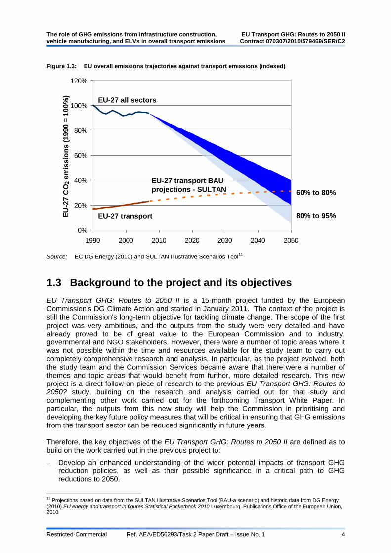
Figure 1.2 shows the baseline, as projected by SULTAN. This is consistent with the range of results from other models and tools, although many of these only project to 20308. Clearly, the predicted continued growth in the EU-27‟s GHG emissions from transport has the potential to prevent the EU meeting the long-term GHG emission reduction targets that the European Council supports, if no action is taken to reduce these emissions. Figure 1.3 demonstrates that on current trends, transport emissions could be around 30% of economy-wide 1990 GHG emissions by 20509. Whilst simplistic, in that it assumes linear reductions, the figure demonstrates that there is clearly a need for additional policy instruments to stimulate the take up of technical and non-technical options that could potentially reduce transport‟s GHG emissions. The EEA believes that all available policy instruments need to be used to achieve the ambitious GHG reduction targets10.
8 See Appendix 19 SULTAN: Development of an Illustrative Scenarios Tool for Assessing Potential Impacts of Measures on EU
transport GHG for details of the assumptions used and approach taken in the SULTAN Illustrative Scenarios Tool to projecting business as usual GHG emissions; also see http://www.eutransportghg2050.eu 9 The emissions included in this figure – for both the economy-wide emissions and those of the transport sector – include
emissions from international aviation and maritime transport, in addition to emissions from “domestic” EU transport. 10
EEA (2009) Towards a resource-efficient transport system – TERM 2009: indicators tracking transport and environment in the European Union, EEA Report No2/2010, Copenhagen.
The role of GHG emissions from infrastructure construction, EU Transport GHG: Routes to 2050 II vehicle manufacturing, and ELVs in overall transport emissions Contract 070307/2010/579469/SER/C2
Restricted-Commercial Ref. AEA/ED56293/Task 2 Paper Draft – Issue No. 1 4
Figure 1.3: EU overall emissions trajectories against transport emissions (indexed)
0%
20%
40%
60%
80%
100%
120%
1990 2000 2010 2020 2030 2040 2050
EU
-27
CO
2 e
mis
sio
ns
(1
99
0 =
10
0%
)
Source: EC DG Energy (2010) and SULTAN Illustrative Scenarios Tool
11
1.3 Background to the project and its objectives
EU Transport GHG: Routes to 2050 II is a 15-month project funded by the European Commission's DG Climate Action and started in January 2011. The context of the project is still the Commission's long-term objective for tackling climate change. The scope of the first project was very ambitious, and the outputs from the study were very detailed and have already proved to be of great value to the European Commission and to industry, governmental and NGO stakeholders. However, there were a number of topic areas where it was not possible within the time and resources available for the study team to carry out completely comprehensive research and analysis. In particular, as the project evolved, both the study team and the Commission Services became aware that there were a number of themes and topic areas that would benefit from further, more detailed research. This new project is a direct follow-on piece of research to the previous EU Transport GHG: Routes to 2050? study, building on the research and analysis carried out for that study and complementing other work carried out for the forthcoming Transport White Paper. In particular, the outputs from this new study will help the Commission in prioritising and developing the key future policy measures that will be critical in ensuring that GHG emissions from the transport sector can be reduced significantly in future years. Therefore, the key objectives of the EU Transport GHG: Routes to 2050 II are defined as to build on the work carried out in the previous project to:
- Develop an enhanced understanding of the wider potential impacts of transport GHG reduction policies, as well as their possible significance in a critical path to GHG reductions to 2050.
11
Projections based on data from the SULTAN Illustrative Scenarios Tool (BAU-a scenario) and historic data from DG Energy (2010) EU energy and transport in figures Statistical Pocketbook 2010 Luxembourg, Publications Office of the European Union, 2010.
EU-27 all sectors
EU-27 transport
EU-27 transport BAU
projections - SULTAN 60% to 80%
80% to 95%
EU Transport GHG: Routes to 2050 II The role of GHG emissions from infrastructure construction, Contract 070307/2010/579469/SER/C2 vehicle manufacturing, and ELVs in overall transport emissions
Restricted-Commercial Ref. AEA/ED56293/Task 2 Paper Draft – Issue No. 1 5
- Further develop the SULTAN illustrative scenarios tool to enhance its usefulness as a policy scoping tool and carry out further scenario analysis in support of the new project;
- Use the new information in the evaluation of a series of alternative pathways to transport GHG reduction for 2050, in the context of the 50-70% reduction target for transport from the European Commission's Roadmap for moving to a competitive low carbon economy in 205012;
As before, given the timescales being considered, the project will take a quantitative approach to the analysis where possible, and a qualitative approach where this is not feasible. The project has been structured against a number tasks, which are as follows:
Task 1: Development of a better understanding of the scale of co-benefits associated with transport sector GHG reduction policies;
Task 2: The role of GHG emissions from infrastructure construction, vehicle manufacturing, and ELVs in overall transport sector emissions;
Task 3: Exploration of the knock-on consequences of relevant potential policies;
Task 4: Exploration of the potential for less transport-intensive paths to societal goals;
Task 5: Identification of the major risks/uncertainties associated with the achievability of the policies and measures considered in the illustrative scenarios;
Task 6: Further development of the SULTAN tool and illustrative scenarios;
Task 7: Exploration of the interaction between the policies that can be put in place prior to 2020 and those achievable later in the time period;
Task 8: Development of a better understanding of the cost effectiveness of different policies and policy packages;
Task 9: Stakeholder engagement: organisation of technical level meetings for experts and stakeholders;
Task 10: Hosting the existing project website and its content;
Task 11: Ad-hoc work requests to cover work beyond that covered in the rest of the work plan.
As in the previous project, stakeholder engagement is an important element of the project. The following meetings are being scheduled:
A large stakeholder meeting currently planned for June 2011 at which the new project will be introduced to stakeholders and interim results presented.
A series of four Technical Focus Group meetings TBC. These are currently scheduled to be held at the start of May 2011 and in November 2011.
A second large stakeholder meeting at which the draft final findings of the project will be presented and discussed, anticipated to be held in February 2012.
As part of the project a number of papers will be produced, all of which will be made available on the project‟s website in draft and then final form, as will all of the presentations from the project‟s meetings.
12
Communication from the Commission to the European Parliament, the Council, the European Economic and Social Committee and the Committee of the Regions, A Roadmap for moving to a competitive low carbon economy in 2050, COM(2011) 112 final. Available from DG Climate Actions website at: http://ec.europa.eu/clima/policies/roadmap/index_en.htm

The role of GHG emissions from infrastructure construction, EU Transport GHG: Routes to 2050 II vehicle manufacturing, and ELVs in overall transport emissions Contract 070307/2010/579469/SER/C2
Restricted-Commercial Ref. AEA/ED56293/Task 2 Paper Draft – Issue No. 1 6
1.4 Background and purpose of the paper
The objective of this paper “The role of GHG emissions from infrastructure construction, vehicle manufacturing, and ELVs in overall transport sector emissions” is to better understand the significance of these emissions and their possible influence on designing optimal routes to long-term GHG reductions from transport. To date, transport sector emissions have been dominated by direct emissions associated with the operational use of vehicles. Previous research in the last ten years has shown that for passenger cars, GHG emissions from vehicle use account for approximately 80% of total life-cycle emissions. Many studies have indicated that the usage phase dominates even further for other modes of transport such as trains, aircraft, and ships, all of which have much longer lifetimes than road transport vehicles. However, there is a need to understand this in more detail and expand the scope of the analysis as some policy options may have unintended impacts on total GHG emissions that may not be immediately obvious if the emissions analysis solely focuses on in-use emissions. In the following sections, we set out our understanding of why analysis of the role of GHG emissions from infrastructure construction and maintenance, vehicle manufacturing, and vehicle disposal (end of life vehicles) is important in the context of this new study.
1.5 Structure of the paper
Following this introduction this paper is structured according to the following further 6 chapters:
2. General Information: This section a summary of the general information relevant to the analysis, including current and likely future development of GHG emission factors for energy carriers and materials.
3. Infrastructure: This section provides a review and analysis of existing evidence on the GHG emissions associated with constructing and maintaining transport infrastructure.
4. Vehicle Manufacturing: This section provides a review and analysis of existing evidence on the GHG emissions associated with the manufacture and maintenance of road vehicles, rail rolling stock, aircraft and ships.
5. Vehicle Disposal: This section provides a review and analysis of existing evidence on the GHG emissions associated with the end of life disposal of road vehicles, rail rolling stock, aircraft and ships.
6. Reaching Optimal Solutions: In this section there is an overall comparison of different transport modes, and an assessment of the possible impacts of including emissions from infrastructure and vehicle production and disposal in the relative performance of different scenario options for reducing GHG emissions in the long term to 2050.
7. Summary of Key Findings and Conclusions: This section provides a final summary of the key findings from the analysis and the conclusions that may be drawn for the rest of the work.

EU Transport GHG: Routes to 2050 II The role of GHG emissions from infrastructure construction, Contract 070307/2010/579469/SER/C2 vehicle manufacturing, and ELVs in overall transport emissions
Restricted-Commercial Ref. AEA/ED56293/Task 2 Paper Draft – Issue No. 1 7
2 General Information
Objectives: The purpose of this section is to provide a summary of the general information relevant to the analysis, i.e.:
Current and likely future development of the GHG intensity of fuels/energy carriers used in the construction and recycling/disposal of infrastructure and vehicles;
Current emission factors for the production of materials (/ key components) used in the construction of vehicles and infrastructure and indications of potential future changes in these;
Summary of Main Findings
To be completed for draft after focus group meeting on 4th May 2011
2.1 General emission factors for energy use
Life cycle estimates for different activities and components in the LCA literature invariably use different assumptions on the carbon intensity of energy consumed as a result of different activities or processes. Where possible it is desirable to normalise literature estimates, or utilise consistent assumptions in the development of new estimates for activities. In addition it is expected that the carbon intensity of different energy carriers will change markedly in the future in Europe in the process of moving towards the attainment of long-term GHG reduction targets. Emissions factors for a range of fuels (direct and indirect) were developed for the SULTAN tool in the previous Routes to 2050 study, presented in Table 2.1. These emission factors have been utilised where possible/appropriate in order to provide a unified set of assumptions for calculations carried out as part of the analysis for this paper.
Table 2.1: Fuel GHG emission factors defined in SULTAN (kgCO2e/kWh)
Fuel direct GHG emissions factor, kgCO2e/kWh
2010 2015 2020 2030 2040 2050
Electricity 0.0000 0.0000 0.0000 0.0000 0.0000 0.0000
Hydrogen 0.0000 0.0000 0.0000 0.0000 0.0000 0.0000
Gas 0.2030 0.2030 0.2030 0.2030 0.2030 0.2030
Fuel indirect GHG emissions factor, kgCO2e/kWh
2010 2015 2020 2030 2040 2050
Electricity 0.3477 0.3057 0.2636 0.1705 0.0670 0.0250
Hydrogen 0.3540 0.3541 0.3543 0.2824 0.0943 0.0347
Gas 0.0301 0.0231 0.0161 0.0161 0.0161 0.0161
Fuel lifecycle GHG emissions factor, kgCO2e/kWh
2010 2015 2020 2030 2040 2050
Electricity 0.3477 0.3057 0.2636 0.1705 0.0670 0.0250
Hydrogen 0.3540 0.3541 0.3543 0.2824 0.0943 0.0347
Gas 0.2331 0.2261 0.2191 0.2191 0.2191 0.2191

The role of GHG emissions from infrastructure construction, EU Transport GHG: Routes to 2050 II vehicle manufacturing, and ELVs in overall transport emissions Contract 070307/2010/579469/SER/C2
Restricted-Commercial Ref. AEA/ED56293/Task 2 Paper Draft – Issue No. 1 8
2.2 General emission factors for raw material production and for material recycling / other disposal
2.2.1 Approaches for accounting for material recycling
In assessing the embodied energy or emissions (or related environmental lifecycle assessment) of transport vehicles and infrastructure it is important to account correctly and consistently (as far as possible) for the method/impacts of recycling. According to Hammond, G., and Jones, C (2011), there is no single universally acceptable method which is, in part, why the subject is so widely debated and methods regularly contested. The subject is also discussed in some detail in Jones (2009). There are broadly three types of methods that can be adopted:
1. Recycled content approach (100:0 method) 2. Substitution method (also known as closed loop system expansion, or 0:100 method) 3. 50:50 method (50:50)
There are advantages and disadvantages of each approach and it is important to consider the boundaries of a study (e.g. cradle‐to‐gate, cradle‐to‐grave) to ensure the selection of an appropriate method. Most studies calculate with the use of recycled materials in the production/construction phase and therefore apply emissions of recycled materials within the initial calculations. As a consequence, these studies allocate recycling energy/emissions benefits to the recycled products. Other studies use the substitution method and calculate with virgin materials energy/emissions factors and apply a recycling stage in the end, with allocation of recycling credits at this point. In reality the true impacts are likely somewhere in-between and the 50:50 method is based on a (relatively arbitrary) mid-point between the two extremes.
2.2.2 Current
This section summarises a set of general emission factors that have been identified for use in this Task 2 analysis for selected raw materials that may be used in the production and construction and maintenance of vehicles and transportation infrastructure. These emission factors may be used in the calculation of embedded emissions of infrastructure, vehicles and disposal for each of the transport modes in the subsequent subtasks. Where data was available, emissions factors have been identified for:
Material production: typical average, virgin and recycled values.
Material disposal: recycling and landfill.
Typical recycling rates: average (global) and automotive (current and future – 2030). Recycling rates within the materials summary table have been taken from the TREMOVE model.
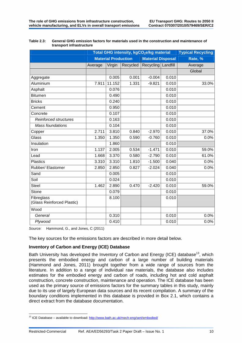
The following Table 2.2 and Table 2.3 present summaries of current emission factors for materials used in road vehicles/trains/aircraft/ships and in the construction and maintenance of transport infrastructure the will be used where appropriate in analysis for this project task.

EU Transport GHG: Routes to 2050 II The role of GHG emissions from infrastructure construction, Contract 070307/2010/579469/SER/C2 vehicle manufacturing, and ELVs in overall transport emissions
Restricted-Commercial Ref. AEA/ED56293/Task 2 Paper Draft – Issue No. 1 9
Table 2.2: General GHG emission factors for materials used in road vehicles, trains, aircraft and ships
Total GHG intensity, kgCO2e/kg material Typical Recycling Primary
Material Production Material Disposal Rate, % Source
Average Virgin Recycled Recycling Landfill Average Automotive
Global Current 2030
Aluminium 7.911 11.152 1.331 -9.821 0.010 33.0% 63.0% 98.0% (1)
Composites
SMC 8.000 8.000 0.010 n.d. 0.0% 0.0% (1)
Glass FRP 8.000 8.000 0.010 n.d. 0.0% 0.0% (1)
Carbon FRP 22.000 22.000 0.010 n.d. 0.0% 0.0% (1)
Copper 2.711 3.810 0.840 -2.970 0.010 37.0% 41.0% 80.0% (2)
Glass 1.350 1.350 0.590 -0.760 0.010 n.d. 10.0% 60.0% (2)
Lead 1.668 3.370 0.580 -2.790 0.010 61.0% 98.0% 100.0% (2)
Li-ion batteries 30.963 n.d. n.d. n.d. (3)
Magnesium 46.050 61.800 30.300 -31.500 0.010 50.0% 63.0% 100.0% (1))
NiMH batteries 23.963 n.d. n.d. n.d. (3)
Lubricating Oil 1.005 1.005 0.471 -0.534 3.939 n.d. 98.0% 98.0% (4)
Plastics (2)
ABS 3.760 3.760 2.260 -1.500 0.040 n.d. 12.0% 95.0% (2)
Polyamide (PA, Nylon) 9.140 9.140 7.640 -1.500 0.040 n.d. 27.0% 100.0% (2)
Polycarbonate 7.620 7.620 6.120 -1.500 0.040 n.d. - - (2)
Polyethylene (PE) 2.540 2.540 1.040 -1.500 0.040 n.d. 27.0% 95.0% (2)
Polyethylene terephthalate (PET)
2.540 2.540 1.040 -1.500 0.040 n.d. 27.0% 95.0% (2)
Polypropylene (PP) 4.490 4.490 2.795 -1.695 0.040 n.d. 27.0% 95.0% (2)
Polyurethane (PUR) 4.840 4.840 3.340 -1.500 0.040 n.d. 27.0% 95.0% (2)
PVC 3.100 3.100 1.980 -1.120 0.040 n.d. 12.0% 95.0% (2)
Other plastics 3.310 3.310 1.810 -1.500 0.040 n.d. 5.0% 80.0% (2)
Rubber/ Elastomer 2.850 2.850 0.827 -2.024 0.040 n.d. 82.0% 85.0% (2)
Steel
Flat carbon steel 1.487 2.355 0.884 -1.471 0.010 59.0% 100.0% 100.0% (1)
Long & special steel 1.292 2.160 0.689 -1.471 0.010 59.0% 61.0% 91.0% (1)
Cast iron 1.137 2.005 0.534 -1.471 0.010 59.0% 99.0% 99.0% (1)
Textile 19.294 19.294 15.494 -3.800 0.300 n.d. 45.0% 80.0% (5)
Wood
Plywood 0.410 0.010 - - (2)
General 0.310 0.010 - - (2)
Zinc 3.082 4.180 0.520 -3.660 0.010 30.0% 38.0% 90.0% (2)
Source: (1) WAS (2010); (2) Hammond, G., and Jones, C (2011); (3) AEA/CE (2010); (4) SimaPro (2007);
(5) DCF (2010).
The role of GHG emissions from infrastructure construction, EU Transport GHG: Routes to 2050 II vehicle manufacturing, and ELVs in overall transport emissions Contract 070307/2010/579469/SER/C2
Restricted-Commercial Ref. AEA/ED56293/Task 2 Paper Draft – Issue No. 1 10
Table 2.3: General GHG emission factors for materials used in the construction and maintenance of transport infrastructure
Total GHG intensity, kgCO2e/kg material Typical Recycling
Material Production Material Disposal Rate, %
Average Virgin Recycled Recycling Landfill Average
Global
Aggregate 0.005 0.001 -0.004 0.010
Aluminium 7.911 11.152 1.331 -9.821 0.010 33.0%
Asphalt 0.076 0.010
Bitumen 0.490 0.010
Bricks 0.240 0.010
Cement 0.950 0.010
Concrete 0.107 0.010
Reinforced structures 0.163 0.010
Mass foundations 0.104 0.010
Copper 2.711 3.810 0.840 -2.970 0.010 37.0%
Glass 1.350 1.350 0.590 -0.760 0.010 0.0%
Insulation 1.860 0.010
Iron 1.137 2.005 0.534 -1.471 0.010 59.0%
Lead 1.668 3.370 0.580 -2.790 0.010 61.0%
Plastics 3.310 3.310 1.810 -1.500 0.040 0.0%
Rubber/ Elastomer 2.850 2.850 0.827 -2.024 0.040 0.0%
Sand 0.005 0.010
Soil 0.024 0.010
Steel 1.462 2.890 0.470 -2.420 0.010 59.0%
Stone 0.079 0.010
Fibreglass (Glass Reinforced Plastic)
8.100 0.010
Wood
General 0.310 0.010 0.0%
Plywood 0.410 0.010 0.0%
Source: Hammond, G., and Jones, C (2011)
The key sources for the emissions factors are described in more detail below.
Inventory of Carbon and Energy (ICE) Database
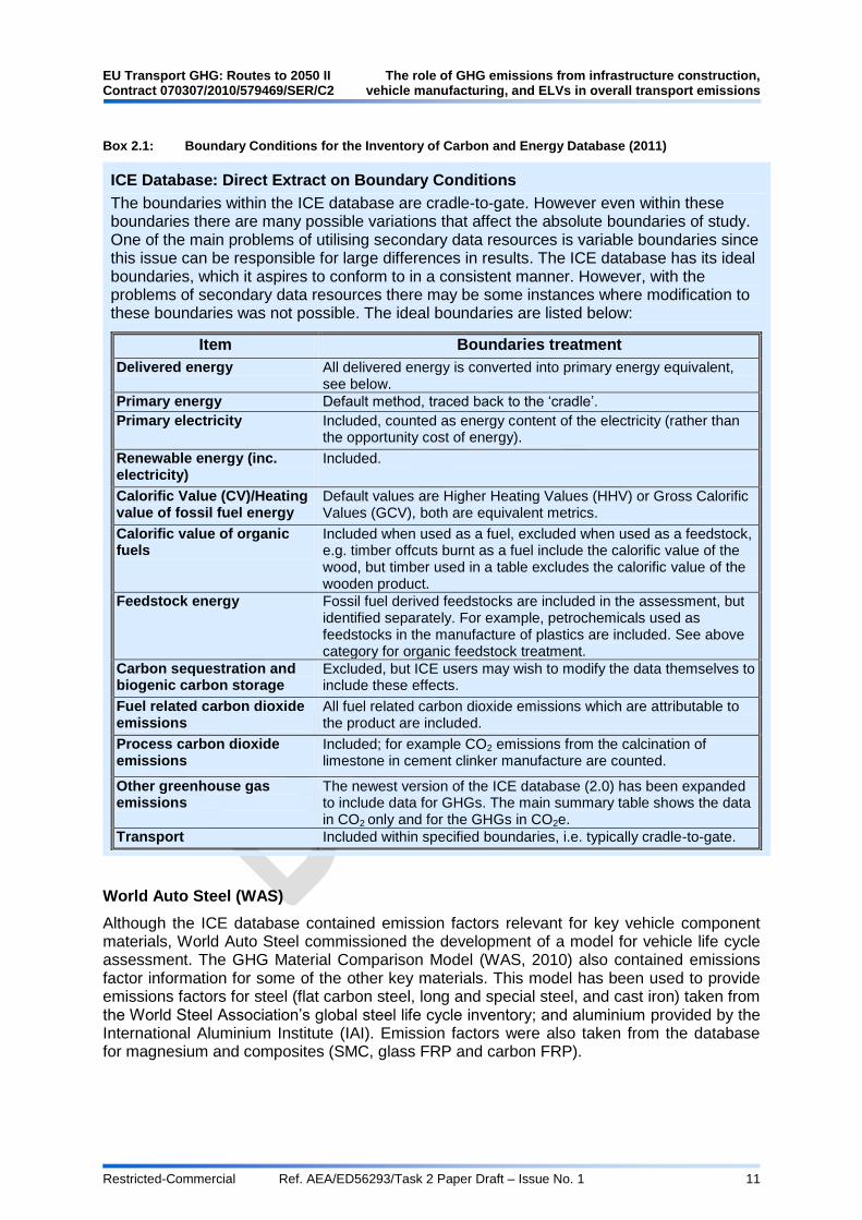
Bath University has developed the Inventory of Carbon and Energy (ICE) database13, which presents the embodied energy and carbon of a large number of building materials (Hammond and Jones, 2011) brought together from a wide range of sources from the literature. In addition to a range of individual raw materials, the database also includes estimates for the embodied energy and carbon of roads, including hot and cold asphalt construction, concrete construction, maintenance and operation. The ICE database has been used as the primary source of emissions factors for the summary tables in this study, mainly due to its use of largely European data sources and its recent compilation. A summary of the boundary conditions implemented in this database is provided in Box 2.1, which contains a direct extract from the database documentation.
13
ICE Database – available to download: http://www.bath.ac.uk/mech-eng/sert/embodied/
EU Transport GHG: Routes to 2050 II The role of GHG emissions from infrastructure construction, Contract 070307/2010/579469/SER/C2 vehicle manufacturing, and ELVs in overall transport emissions
Restricted-Commercial Ref. AEA/ED56293/Task 2 Paper Draft – Issue No. 1 11
Box 2.1: Boundary Conditions for the Inventory of Carbon and Energy Database (2011)
ICE Database: Direct Extract on Boundary Conditions
The boundaries within the ICE database are cradle-to-gate. However even within these boundaries there are many possible variations that affect the absolute boundaries of study. One of the main problems of utilising secondary data resources is variable boundaries since this issue can be responsible for large differences in results. The ICE database has its ideal boundaries, which it aspires to conform to in a consistent manner. However, with the problems of secondary data resources there may be some instances where modification to these boundaries was not possible. The ideal boundaries are listed below:
Item Boundaries treatment
Delivered energy All delivered energy is converted into primary energy equivalent, see below.
Primary energy Default method, traced back to the „cradle‟.
Primary electricity Included, counted as energy content of the electricity (rather than the opportunity cost of energy).
Renewable energy (inc. electricity)
Included.
Calorific Value (CV)/Heating value of fossil fuel energy
Default values are Higher Heating Values (HHV) or Gross Calorific Values (GCV), both are equivalent metrics.
Calorific value of organic fuels
Included when used as a fuel, excluded when used as a feedstock, e.g. timber offcuts burnt as a fuel include the calorific value of the wood, but timber used in a table excludes the calorific value of the wooden product.
Feedstock energy Fossil fuel derived feedstocks are included in the assessment, but identified separately. For example, petrochemicals used as feedstocks in the manufacture of plastics are included. See above category for organic feedstock treatment.
Carbon sequestration and biogenic carbon storage
Excluded, but ICE users may wish to modify the data themselves to include these effects.
Fuel related carbon dioxide emissions
All fuel related carbon dioxide emissions which are attributable to the product are included.
Process carbon dioxide emissions
Included; for example CO2 emissions from the calcination of limestone in cement clinker manufacture are counted.
Other greenhouse gas emissions
The newest version of the ICE database (2.0) has been expanded to include data for GHGs. The main summary table shows the data in CO2 only and for the GHGs in CO2e.
Transport Included within specified boundaries, i.e. typically cradle-to-gate.
World Auto Steel (WAS)
Although the ICE database contained emission factors relevant for key vehicle component materials, World Auto Steel commissioned the development of a model for vehicle life cycle assessment. The GHG Material Comparison Model (WAS, 2010) also contained emissions factor information for some of the other key materials. This model has been used to provide emissions factors for steel (flat carbon steel, long and special steel, and cast iron) taken from the World Steel Association‟s global steel life cycle inventory; and aluminium provided by the International Aluminium Institute (IAI). Emission factors were also taken from the database for magnesium and composites (SMC, glass FRP and carbon FRP).
The role of GHG emissions from infrastructure construction, EU Transport GHG: Routes to 2050 II vehicle manufacturing, and ELVs in overall transport emissions Contract 070307/2010/579469/SER/C2
Restricted-Commercial Ref. AEA/ED56293/Task 2 Paper Draft – Issue No. 1 12
SimaPro (2007)
Emission factors for lubricating oil were taken fro the SimaPro Ecoinvent database (2007). The database comprises of approximately 4,000 datasets for products, services and processes often used in LCA studies.
AEA/CE (2010)
The dataset compiled through work carried out by AEA/CE Delft for DG CLIMA has been used to provide emission factors for Li-ion batteries and NiMH batteries.
2.2.3 Future development
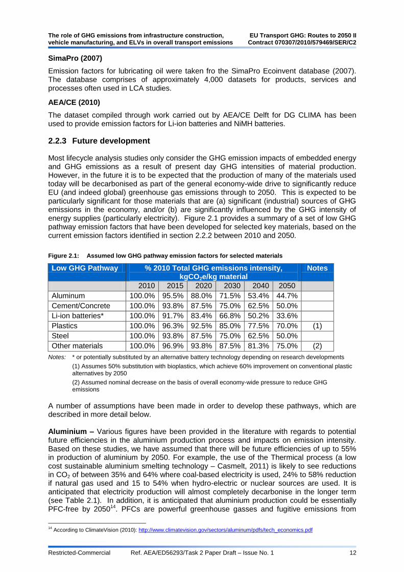
Most lifecycle analysis studies only consider the GHG emission impacts of embedded energy and GHG emissions as a result of present day GHG intensities of material production. However, in the future it is to be expected that the production of many of the materials used today will be decarbonised as part of the general economy-wide drive to significantly reduce EU (and indeed global) greenhouse gas emissions through to 2050. This is expected to be particularly significant for those materials that are (a) significant (industrial) sources of GHG emissions in the economy, and/or (b) are significantly influenced by the GHG intensity of energy supplies (particularly electricity). Figure 2.1 provides a summary of a set of low GHG pathway emission factors that have been developed for selected key materials, based on the current emission factors identified in section 2.2.2 between 2010 and 2050.
Figure 2.1: Assumed low GHG pathway emission factors for selected materials
Low GHG Pathway % 2010 Total GHG emissions intensity, kgCO2e/kg material
Notes
2010 2015 2020 2030 2040 2050
Aluminum 100.0% 95.5% 88.0% 71.5% 53.4% 44.7%
Cement/Concrete 100.0% 93.8% 87.5% 75.0% 62.5% 50.0%
Li-ion batteries* 100.0% 91.7% 83.4% 66.8% 50.2% 33.6%
Plastics 100.0% 96.3% 92.5% 85.0% 77.5% 70.0% (1)
Steel 100.0% 93.8% 87.5% 75.0% 62.5% 50.0%
Other materials 100.0% 96.9% 93.8% 87.5% 81.3% 75.0% (2)
Notes: * or potentially substituted by an alternative battery technology depending on research developments
(1) Assumes 50% substitution with bioplastics, which achieve 60% improvement on conventional plastic alternatives by 2050
(2) Assumed nominal decrease on the basis of overall economy-wide pressure to reduce GHG emissions
A number of assumptions have been made in order to develop these pathways, which are described in more detail below. Aluminium – Various figures have been provided in the literature with regards to potential future efficiencies in the aluminium production process and impacts on emission intensity. Based on these studies, we have assumed that there will be future efficiencies of up to 55% in production of aluminium by 2050. For example, the use of the Thermical process (a low cost sustainable aluminium smelting technology – Casmelt, 2011) is likely to see reductions in CO2 of between 35% and 64% where coal-based electricity is used, 24% to 58% reduction if natural gas used and 15 to 54% when hydro-electric or nuclear sources are used. It is anticipated that electricity production will almost completely decarbonise in the longer term (see Table 2.1). In addition, it is anticipated that aluminium production could be essentially PFC-free by 205014. PFCs are powerful greenhouse gasses and fugitive emissions from
14
According to ClimateVision (2010): http://www.climatevision.gov/sectors/aluminum/pdfs/tech_economics.pdf

EU Transport GHG: Routes to 2050 II The role of GHG emissions from infrastructure construction, Contract 070307/2010/579469/SER/C2 vehicle manufacturing, and ELVs in overall transport emissions
Restricted-Commercial Ref. AEA/ED56293/Task 2 Paper Draft – Issue No. 1 13
aluminium production currently account for around 9-18% of total GHG from aluminium production (WAS, 2010). Cement/concrete – Reductions in GHG from cement production have been assumed to reach 50% of 2010 levels by 2050. Best available technology is currently used in cement production, so any future savings are going to have to be achieved through the use of new technologies. The IEA (2009) developed a Cement Technology Roadmap detailing the potential developments in the technology and production process and carbon emissions reduction to 2050. The roadmap found that four key levers available to the cement industry that would enable emissions reductions in the production process, which included thermal and electric efficiency; alternative fuel use; clinker substitution; and carbon capture and storage. Roadmap indicators suggest up to a 56% reduction in emissions by 2050 might be achieved. Li-ion batteries – Figures for the potential for reduction in GHG emissions from the production of lithium ion batteries have been estimated based upon the difference between the average and the lowest figures from the literature, as summarised in Table 2.4 below.
Table 2.4: Estimates of GHG intensity NiMH and Li-ion batteries based on sources from the literature
Reference Battery Type Battery kgCO2e/kg
Samaras (2008)15
NiMH 23.1
Li-ion 24.0
Zackrissona (2010)16
Li-ion (water as solvent) 53.2
Li-ion (NMP as solvent) 33.2
AEA (2007)17
NiMH 24.8
Li-ion 39.9
Helms (2010)18
Li-ion 25.0
Notter (2010)19
Li-ion 10.4
Average NiMH 24.0
Li-ion 31.0
Lowest Li-ion 10.4
Notes: Estimates have been derived from information provided in the different reference sources. Plastics – An overall 30% improvement in emissions efficiency has been assumed for plastics compared to 2010. This is based on the assumptions that 50% of existing plastics can be substituted by bioplastic alternatives by 2050, and these bioplastics achieve on average 60% reduction in GHG compared to conventional plastics. 30% is a conservative estimate, but takes into account the uncertainties relating to the feasibility of reductions to conventional plastics and the availability of/substitution with bioplastic alternatives. Steel – GHG intensity improvements on 2010 of up to 50% by 2050 have been assumed for steel, which includes the use of a range of breakthrough technologies and processes. Some of the largest global steel producers are committed to reducing carbon emissions from their processes. For example, Corus/Tata Steel Group (6th largest global steel producer and 2nd largest steel producer in Europe) is committed to reducing carbon emissions from the steel
15
Life Cycle Assessment of Greenhouse Gas Emissions, from Plug-in Hybrid Vehicles: Implications for Policy, Constantine Samaras, and Kyle Meisterling, Environ. Sci. Technol., 2008, 42 (9), 3170-3176 • DOI: 10.1021/es702178s • Publication Date (Web): 05 April 2008 16
Zackrissona, 2010. Mats Zackrissona, Lars Avellána, and Jessica Orleniusb, Life cycle assessment of lithium-ion batteries for plug-in hybrid electric vehicles – Critical issues. 2010. 17
Hybrid Electric and Battery Electric Vehicles, Technology, Costs and benefits, work carried out by AEA for Sustainable Energy Ireland, November 2007 18
"Helms et al, 2010. Electric vehicle and plug-in hybrid energy efficiency and life cycle emissions, H. Helms, M. Pehnt, U. Lambrecht and A. Liebich, Ifeu – Institut für Energie- und Umweltforschung, Wilckensstr. 3, D-69120 Heidelberg. 18th International Symposium Transport and Air Pollution Session 3: Electro and Hybrid Vehicles, page 113 from 274. 2010." 19
Domenic A. Notter et al., Contribution of Li-Ion Batteries to the Environmental Impact of Electric Vehicles, EMPA, Switzerland, in Environ. Sci. Technol. 2010, 44, 6550–6556

The role of GHG emissions from infrastructure construction, EU Transport GHG: Routes to 2050 II vehicle manufacturing, and ELVs in overall transport emissions Contract 070307/2010/579469/SER/C2
Restricted-Commercial Ref. AEA/ED56293/Task 2 Paper Draft – Issue No. 1 14
production process by 20% compared to 1990 levels by 2020. A number of new technologies are also being explored within the steel industry which will also achieve savings in carbon emissions. These include top gas recycling blast furnaces, Hisarna, ULCORED and electrolysis (Brookes, 2008; ULCOS, 2010). The first three of these options should be combined with carbon capture and storage (CCS) to achieve the 50% savings. Allwood and Cullen (2009) also discuss a range of technologies and strategies that could reduce carbon emissions from the steel making process by 2050. These options include CCS (-27%), non-destructive recycling (-48%), reduced demand (-50%) and radical efficiency (-50%). Other materials – The information for other materials varies greatly, with some very large and some very small efficiencies to be gained over time. Therefore, a nominal decrease in emissions intensity has been assumed for the GHG pathway of up to 25% by 2050.
2.3 References
Allwood, J., and Cullen, J. (2009) Steel, aluminium and carbon: alternative strategies for meeting the 2050 carbon emissions targets, R‟09, Davos, 15th September 2009. Department of Engineering University of Cambridge, UK. http://www.lcmp.eng.cam.ac.uk/wp-content/uploads/JMA-R09-Davos-Sept-09s.pdf
Brooks, P (2008) Using technology to reduce carbon intensity in production/manufacturing – Presentation to CBI climate change summit. http://www.slideshare.net/thecbi/using-technology-to-reduce-carbon-intensity-in-productionmanufacturing-dr-paul-brooks-director-environment-climate-change-corus-presentation
Casmelt (2011) Energy Requirements and CO2 Generation, Casmelt, Australia. http://www.calsmelt.com/energy-environmental.html
Frost & Sullivan (2010) Global Electric Vehicles Lithium-ion Battery Second Life and Recycling Market Analysis, Frost & Sullivan. http://www.frost.com/prod/servlet/report-toc.pag?repid=M5B6-01-00-00-00
Hammond, G., and Jones, C (2011) Inventory of Carbon & Energy (ICE) Version 2.0, University of Bath, UK. http://www.bath.ac.uk/mech-eng/sert/embodied/
IEA (2009) Cement Technology Roadmap 2009 – Carbon Emission Reductions up to 2050, International Energy Agency and World Business Council for Sustainable Development. http://iea.org/papers/2009/Cement_Roadmap.pdf
Jones (2009). “Embodied Impact Assessment: The Methodological Challenge of Recycling at the End of Building Lifetime”, by Craig I. Jones, Construction Information Quarterly, Volume: 11 | Issue: 3, CONSTRUCTION PAPER 248. 2009.
Nemry, F., and Bons, M (2010) Plug-in Hybrid and Battery Electric Vehicles: Market Penetration Scenarios of Electric Drive Vehicles, European Commission/Joint Research Council. http://ftp.jrc.es/EURdoc/JRC58748_TN.pdf
ULCOS (2010) Ultra Low CO2 Steelmaking – Where we are today, Ultra-Low Carbon dioxide (CO2) Steelmaking http://www.ulcos.org/en/research/where_we_are_today.php
WAS (2010) GHG Material Comparison Model, World Auto Steel. http://www.worldautosteel.org/Projects/LCA-Study/2010-UCSB-model.aspx
EU Transport GHG: Routes to 2050 II The role of GHG emissions from infrastructure construction, Contract 070307/2010/579469/SER/C2 vehicle manufacturing, and ELVs in overall transport emissions
Restricted-Commercial Ref. AEA/ED56293/Task 2 Paper Draft – Issue No. 1 15
3 Infrastructure
Objectives: The purpose of this sub-task was to understand the scale of the impacts of GHG emissions associated with the creation of new transport infrastructure in the context of total transport sector emissions. This will include review and analysis of existing evidence on the GHG emissions associated with constructing:
New roads;
New conventional and high-speed railway lines;
New airports;
New port infrastructure for ships; and
New fuel/energy carrier infrastructure.
Summary of Main Findings
To be completed for draft after focus group meeting on 4th May 2011
3.1 Road Transport
3.1.1 Summary of information from the literature
Current status Road infrastructure typically consists of the roads themselves, but can also include other elements such as bridges and lighting. Although the GHG emissions attributed to the road infrastructure itself are currently not the main contributor to the total GHG emissions from the total system of road transport they are not negligible. The evidence shows that emissions related to road construction, maintenance, operation and end-of-life may range from just a few per cent to over 10% of total road lifecycle emissions (e.g. Spielmann et al (2007), Stripple (2001)). However, there are also sources that state that 35% to over 40% of the GHG emissions for the full road infrastructure system including vehicle production and use can be attributed to the road construction, maintenance and operation (Chester and Horvath, 2009; CEPAL, 2010). It is likely that in the future the indirect GHG emissions associated with road infrastructure will become increasingly important and significant as direct GHG emissions from road transport decrease as a result of advances in technology, fuel and vehicle manufacturing. In terms of the main methods associated with road infrastructure construction in Europe, the vast majority (95%) of roads are constructed by applying compacted layers of aggregates on top of the subsoil. The aggregates are mainly natural aggregates like gravel and crushed rock (COURAGE, 1999). The aggregate layers are then covered with a top layer which is often made from asphalt and otherwise made from concrete (COURAGE, 1999; COURAGE, 2009). GHG emissions associated with the construction of road infrastructure have been estimated at 9 to 27 kg CO2e.m-1.y-1. This seems to be in the same order as the combined maintenance and operation of the road are (see Table 3.1). In these figures the production, transport and application of pavement materials are included. For concrete pavements, the GHG emissions are mainly related to the use of clinker in the cement, while for asphalt concrete pavements the GHG emissions mainly stem from the production of bitumen and of the asphalt mixture Kellenberger et al (2007). The road construction itself can be attributed to approximately to 50% of the total of construction, maintenance and operation.

The role of GHG emissions from infrastructure construction, EU Transport GHG: Routes to 2050 II vehicle manufacturing, and ELVs in overall transport emissions Contract 070307/2010/579469/SER/C2
Restricted-Commercial Ref. AEA/ED56293/Task 2 Paper Draft – Issue No. 1 16
Figure 3.1 GHG emissions during 40 years of service life of a 13 m wide road in Sweden (adapted from Stripple, 2001).
0.0
0.2
0.4
0.6
0.8
1.0
1.2
1.4
1.6
1.8
2.0
Asphalt road - Hot construction
method
Asphalt road - Cold construction
method
Concrete road
ktC
O2 p
er
km
Construction Maintenance - 40 yrs Operation - 40 yrs
Maintenance is of particular concern in relation to asphalt concrete pavements; the road surface of asphalt concrete pavements is regularly removed and a new layer is subsequently applied. Maintenance actions related to road surfaces includes, in principle, all preventive and corrective maintenance. For highways and motorways, the maintenance of the road surface has a shorter cycle i.e. 10 years than the lifecycle of the total road (30-50 years).GHG emissions related to road maintenance are attributed to the use of materials like bitumen, asphalt mixture and concrete. The GHG emissions are in the order of 1 to 5 kg CO2e.m-1.y-1 (see Table 3.1) and so approximately 20% of those of the initial construction and 10% of the total including construction, maintenance and operation. Higher traffic loads on roads, especially more frequent and higher axle loads, determine the design of the road in terms of the foundation layers, intermediate layers and road surface layers required. Higher traffic loads will in general require more and stronger materials which in their turn will generally lead to higher GHG emissions. There will also be an increased need for maintenance, leading to GHG emissions associated with higher traffic loads (see e.g. Satahaye et al, 2010). It has been estimated by Zhang et al (2008) that the GHG emissions related to congestion due to road surface maintenance activities and the impact of the road surface on vehicle emissions is in the same order of magnitude as the GHG emissions for the maintenance materials and operations (see Figure 3.2).

EU Transport GHG: Routes to 2050 II The role of GHG emissions from infrastructure construction, Contract 070307/2010/579469/SER/C2 vehicle manufacturing, and ELVs in overall transport emissions
Restricted-Commercial Ref. AEA/ED56293/Task 2 Paper Draft – Issue No. 1 17
Figure 3.2 GHG emissions from road surface construction and maintenance for different road surface materials. Congestion includes all construction and maintenance related traffic congestion. Usage includes overlay roughness effects on vehicular travel and fuel consumption during normal traffic flow (after Zhang et al (2008)).
0
1
2
3
4
5
6
7
8
Concrete Cement Composite Hot Asphalt
GH
G E
mis
sio
ns,
ktC
O2e p
er
km
Congestion Useage Construction and Materials Other (EOL)
Another stage that can be distinguished is the operation stage. It includes the lighting of the road, the use of traffic lights and other traffic systems and cleaning and keeping the road ice-free (see e.g. Stripple, 2001). The operation stage contributes about 6-18 kg CO2e.m-1.y-1 (see Table 3.1). This is in the same order as the road construction itself. The contribution to the total of construction, maintenance and operation is approximately 40%. Road lighting significantly contributes to the GHG emissions of the operation stage. According to Stripple (2001), road lighting may consume 95% of the energy for the operation stages and hence may be responsible for the majority of the GHG emissions. However, lighting schemes may differ between countries (see i.e. Figure 3.3), as well as the need for illuminating roads across Europe due to differences in hours of daylight and traffic intensity. As the GHG emissions from lighting are from the use of electricity, the differing electricity mix in European countries will also influence the resulting GHG emissions.

The role of GHG emissions from infrastructure construction, EU Transport GHG: Routes to 2050 II vehicle manufacturing, and ELVs in overall transport emissions Contract 070307/2010/579469/SER/C2
Restricted-Commercial Ref. AEA/ED56293/Task 2 Paper Draft – Issue No. 1 18
Figure 3.3 Image of artificial light at night time in Europe (NASA).
Alternatives to reduce GHG emissions There are a number of methods and processes that could be employed in the road transport sector to reduce the GHG emissions at the road construction stage, including the use of alternative materials. For example, using alternative binders, such as slag cement, is a way to reduce the GHG emissions in concrete pavement. Slag cement has approximately 50% of the GHG emissions of conventional Portland cement. Naturally based pozzolanas occur in volcanic ash or even in treated plant residues may also replace clinker based cements. Pozzolanas contain reactive silica and/or alumina which, when mixed with lime in the presence of water, will set and harden like a cement. Ash from rice husks is an example of such a pozzolana and may be used in road construction (Lennox and McKenzie, 2008). For asphalt concrete pavements the use of recycled asphalt pavement avoids, among others things, the use of primary aggregates and primary bitumen and so reduces GHG emissions. The replacement of primary bitumen may be more important in terms of GHG emissions reduction than the replacement of primary aggregates. Secondary materials that replace natural aggregates in road construction may reduce the GHG emissions related to these aggregates (Chowdhury et al, 2010; Huang et al, 2009). However, some secondary materials like crushed concrete may have higher GHG emissions associated with than natural aggregates do (Chowdhury et al, 2010; Huang et al, 2009). So although certain secondary aggregates do not have a great potential to reduce GHG emissions for road infrastructure, they may have other benefits, such as the reduction of final waste and reduced land use impacts.
EU Transport GHG: Routes to 2050 II The role of GHG emissions from infrastructure construction, Contract 070307/2010/579469/SER/C2 vehicle manufacturing, and ELVs in overall transport emissions
Restricted-Commercial Ref. AEA/ED56293/Task 2 Paper Draft – Issue No. 1 19
The use of bio-fuels in the production of hot asphalt mixtures has been estimated to reduce the GHG emissions with 35% (Head et al, 2010). Another option to reduce the GHG emissions of asphalt concrete is the development of so called „cold asphalt‟. This often takes the form of an asphalt emulsion which can be produced at much lower temperatures and hence lower fuel use than in the production of conventional asphalt concrete. However, in some cases cement is added to these emulsions, which can subsequently increase GHG emissions. The use of bio-based oils and resins in these asphalt emulsions will reduce the GHG emission potential. Some companies are already using bio-based binders that (partially) replace bitumen in the road surface. This may reduce GHG emissions to 50-70% (Colas France, 2009; Colas Switzerland, 2009; and Head et al, 2010). The condition of the road surface can directly influence traffic safety, noise generation and vehicle fuel consumption (Penant, 2008; and Morgan, 2006). Road surface maintenance can therefore be optimised to fulfil GHG emission reductions and other sustainable transport and safety objectives. A promising option for porous asphalt road surfaces seems to be the use of other maintenance schemes based on rejuvenating the road surface instead of removal and reconstruction of the road surface (Head et al, 2010). The amount of emission reduction is not well known but is estimated to be in the range of 5-10%. As lighting contributes greatly to the GHG emissions related to the operation of the road, energy-efficient lighting scenarios (see Figure 3.4) may be a key option for reducing these emissions (Fox, 2007). Optimised lighting may reduce the GHG emissions to roughly 60% of the operation stages emissions. The use of intelligent lighting combined with LED illumination may substantially reduce the energy need with 70% (see LITES, 2010) and will so reduce the GHG emissions related to road lighting. Another development is the decarbonisation of the electricity production in Europe through an increase in the share of renewable sources like wind and hydro power and use of biomass as a fuel for power plants. This may lead to a reduction of the GHG emissions to around 5% of fossil based electricity.

The role of GHG emissions from infrastructure construction, EU Transport GHG: Routes to 2050 II vehicle manufacturing, and ELVs in overall transport emissions Contract 070307/2010/579469/SER/C2
Restricted-Commercial Ref. AEA/ED56293/Task 2 Paper Draft – Issue No. 1 20
Figure 3.4 Impact on lighting scheme on electricity use related GHG emissions. Option 1 is ‘blanket lighting’; option 2A lighting only meets British standards (Fox 2007).
0
10
20
30
40
50
60
Residential Area (Option 1)
Residential Area (Option 1, min. lighting)
Residential Area (Option
2A)
Traffic Route Motorway
kg
CO
2e.m
-1.y
-1
Existing Variable Part Night
Status of current road infrastructure in Europe
In 2009, there were over 56,000 kilometres of motorways and nearly 3.5 million kilometres of other roads in Europe (Eurostat, 2011). The actual totals As some countries as Italy and Greece lack data these numbers will be higher.
3.1.2 Development of emission factors for the analysis
Based on several literature sources GHG emission factors for road construction and road maintenance and operation have been established, and are displayed in Table 3.1. For roads made from asphalt concrete the emission factors identified per meter per year are of similar magnitudes; 8.9 to 10.1 kg CO2e (see Table 3.1). Concrete based roads appear to have an almost twice as high emission factor, but figures for the road surface give an opposite direction. The emission factors for road maintenance and operation show a larger variation. This is most likely related to differences in energy use for lighting.
Table 3.1: Current emission factors for road infrastructure.
Life cycle stage Detail Kg CO2e.m-1
.y-1
Source
Construction Asphalt concrete and concrete
20 10.1 0
Hot asphalt concrete21
10.7 0, 0
Cold asphalt concrete2
9.2 0, 0
Concrete2
26.7 0, 0
Hot asphalt, incl. end-of-life22
8.9 0
20
For total width of average road. 21
For road width of 13 m.
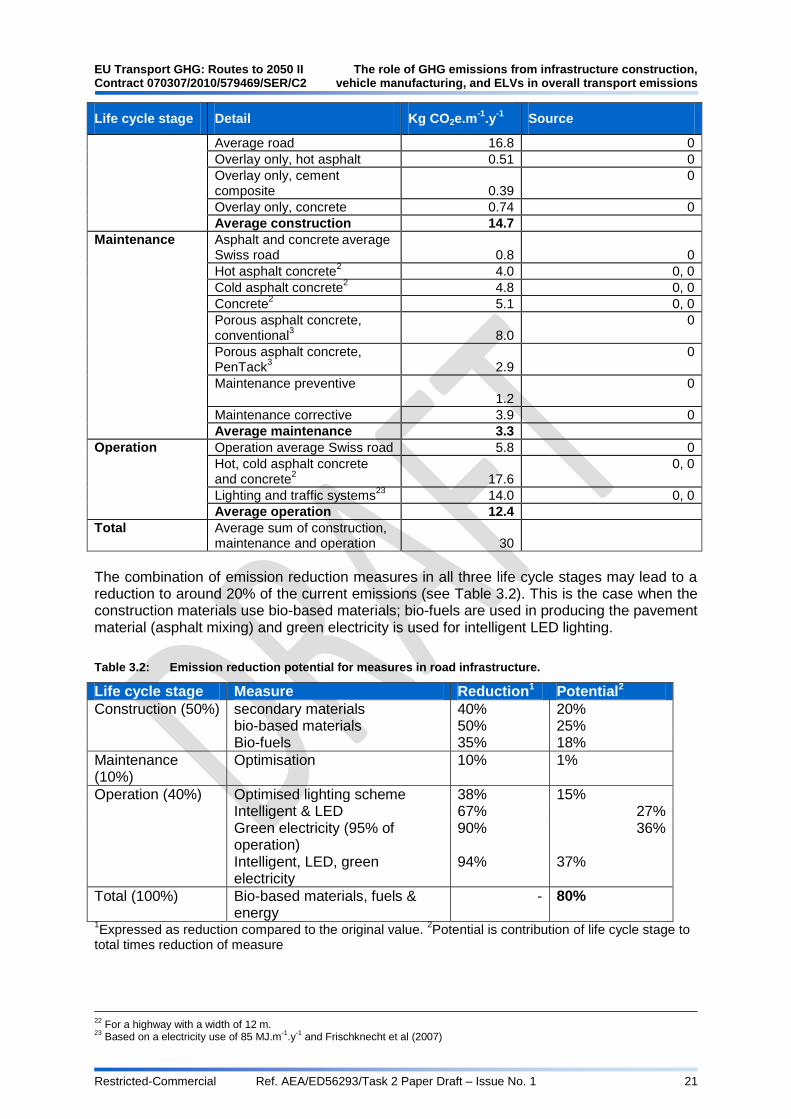
EU Transport GHG: Routes to 2050 II The role of GHG emissions from infrastructure construction, Contract 070307/2010/579469/SER/C2 vehicle manufacturing, and ELVs in overall transport emissions
Restricted-Commercial Ref. AEA/ED56293/Task 2 Paper Draft – Issue No. 1 21
Life cycle stage Detail Kg CO2e.m-1
.y-1
Source
Average road 16.8 0
Overlay only, hot asphalt 0.51 0
Overlay only, cement composite 0.39
0
Overlay only, concrete 0.74 0
Average construction 14.7
Maintenance Asphalt and concrete average
Swiss road 0.8 0
Hot asphalt concrete2
4.0 0, 0
Cold asphalt concrete2
4.8 0, 0
Concrete2
5.1 0, 0
Porous asphalt concrete, conventional
3 8.0
0
Porous asphalt concrete, PenTack
3 2.9
0
Maintenance preventive 1.2
0
Maintenance corrective 3.9 0
Average maintenance 3.3
Operation Operation average Swiss road 5.8 0
Hot, cold asphalt concrete and concrete
2 17.6
0, 0
Lighting and traffic systems23
14.0 0, 0
Average operation 12.4
Total Average sum of construction, maintenance and operation 30
The combination of emission reduction measures in all three life cycle stages may lead to a reduction to around 20% of the current emissions (see Table 3.2). This is the case when the construction materials use bio-based materials; bio-fuels are used in producing the pavement material (asphalt mixing) and green electricity is used for intelligent LED lighting.
Table 3.2: Emission reduction potential for measures in road infrastructure.
Life cycle stage Measure Reduction1 Potential2
Construction (50%) secondary materials 40% 20% bio-based materials 50% 25% Bio-fuels 35% 18%
Maintenance (10%)
Optimisation 10% 1%
Operation (40%) Optimised lighting scheme 38% 15% Intelligent & LED 67% 27% Green electricity (95% of
operation) 90% 36%
Intelligent, LED, green electricity
94% 37%
Total (100%) Bio-based materials, fuels & energy
- 80%
1Expressed as reduction compared to the original value.
2Potential is contribution of life cycle stage to
total times reduction of measure
22
For a highway with a width of 12 m. 23
Based on a electricity use of 85 MJ.m-1.y
-1 and Frischknecht et al (2007)

The role of GHG emissions from infrastructure construction, EU Transport GHG: Routes to 2050 II vehicle manufacturing, and ELVs in overall transport emissions Contract 070307/2010/579469/SER/C2
Restricted-Commercial Ref. AEA/ED56293/Task 2 Paper Draft – Issue No. 1 22
3.1.3 References
CEPAL (2010) Towards low-carbon transportation infrastructures. FAL Bulletin Issue No. 2 8 6 - Numb er 0 6 / 2 0 1 0 Chester M.V., Horvarth M., (2009) Supporting Information For: Environmental Assessment of Passenger Transportation Should Include Infrastructure and Supply Chains. http://iopscience.iop.org/1748-9326/4/2/024008/media/erl9_2_024008suppdata.pdf. Date of last access 13-04-2011 Chowdhury R., Apul D., Fry T. (2010) A life cycle based environmental impacts assessment of construction materials used in road construction. Resources, Conservation and Recycling 54 (2010) 250–255 Colas France, (2009) Developing Silent, Natural, Low Temperature, Recycled Road Products and Techniques. In: Innovative Practices for Greener Roads. IRF. http://www.irfnet.org/files-upload/pdf-files/IRF_BP_Environment_Web.pdf Date of last access 06/04/2011 Colas Switzerland, (2009) Promoting the Widespread Use of VALORCOL. In: Innovative Practices for Greener Roads. IRF. http://www.irfnet.org/files-upload/pdf-files/IRF_BP_Environment_Web.pdf Date of last access 06/04/2011 COURAGE (1999) Final Report COnstruction with Unbound Road Aggregates in Europe. 4th Framework Programme, Contract No.: RO-97-SC.2056. http://www.transport-research.info/Upload/Documents/200310/couragefrep.pdf Date of last access 13-04-2011 COURAGE (2009) Construction with Unbound Road Aggregates in Europe. Transport Research Knowledge Centre - COURAGE - Construction with Unbound Road Aggregates in Europe. Date of last access 13-04-2011 Eurostat (2011) Road, rail and navigable inland waterways networks at regional level. http://appsso.eurostat.ec.europa.eu/nui/show.do?dataset=tran_r_net&lang=en Fox P., (2007) Invest to save – sustainable street lighting, CSS Street Lighting Project SL2/2007. Available at: http://www.theilp.org.uk/uploads/File/Technical/SL2_secure.pdf Date of last access 06/04/2011 Frischknecht, R., Tuchschmid, M., Faist Emmenegger, M.,Bauer, C., Dones, R., (2007) Strommix und Stromnetz. Sachbilanzen von Energiesystemen. Final report No. 6 ecoinvent data v2.0. Editors: Dones R.. Volume: 6. Swiss Centre for LCI, PSI. Dübendorf and Villigen, CH. Gosse C., Smith B., Clarens A., (2010) Greenhouse Gas Emissions in Pavement Management Systems Civil and Environmental Engineering, University of Virginia. Poster http://www.lcacenter.org/LCAX/presentations/118.pdf Date of last Access 18-04-2011 Hammond G., Jones C., (2011) Inventory of Carbon and Energy (ICE). http://people.bath.ac.uk/cj219 Date of last access 06/04/2011 Head M.E., Ligthart T.N., Ansems A.M.M., (2010) LCA of porous with PenTack maintenance system and a comparison with traditional maintenance. TNO report TNO-034-UT-2010-01240_RPT-ML (in Dutch).

EU Transport GHG: Routes to 2050 II The role of GHG emissions from infrastructure construction, Contract 070307/2010/579469/SER/C2 vehicle manufacturing, and ELVs in overall transport emissions
Restricted-Commercial Ref. AEA/ED56293/Task 2 Paper Draft – Issue No. 1 23
Huang Y., Bird R., Heidrich O., (2009) Development of a life cycle assessment tool for construction and maintenance of asphalt pavements. Journal of Cleaner Production 17 (2009) 283–296 Kellenberger D., Althaus H.-J., Jungbluth N., Künniger T., (2007) Life Cycle Inventories of Building Products. Final report ecoinvent data v2.0. Volume: 7. Swiss Centre for LCI, Empa - TSL. Dübendorf, CH. Lennox R., MacKenzie M., (2008) Eco-Road Building for Emerging Economies: An Initial Scan for Promising Alternative Technologies. Global Transport Knowledge Partnership. LITES (2010) Led-based intelligent street lighting for energy saving. http://www.lites-project.eu/ Date of last access 08/04/2011 Morgan P., (2006) Guidance manual for the implementation of low-noise road surfaces. FEHRL Report 2006/02 http://www.trl.co.uk/silvia/Silvia/pdf/silvia_guidance_manual.pdf NASA, Visible Earth: Earth‟s city lights. Data courtesy Marc Imhoff of NASA GSFC and Christopher Elvidge of NOAA NGDC. Image by Craig Mayhew and Robert Simmon, NASA GSFC. http://visibleearth.nasa.gov/view_rec.php?id=1438 Penant C., (2008) A brief review of tyre-pavement interaction and an insight on new regulation on tyre rolling resistance in Europe. Group Michelin. http://www.road-transport-technology.org/HVTT10/Proceeding/Papers/Papers_HVTT/paper_84.pdf Sathaye N., Horvath A., Madanat S., (2010) Unintended impacts of increased truck loads on pavement supply-chain emissions. Transportation Research Part A 44 (2010) 1–15 Spielmann M., Dones R; Bauer C., (2007) Life Cycle Inventories of Transport Services. Final report ecoinvent Data v2.0. Volume: 14. Issue: 0. Swiss Centre for LCI, PSI. Dübendorf and Villigen, CH. Stripple H., (2001) Life Cycle Assessment of Road - A pilot study for inventory analysis. IVL Swedish Environmental Research Institute. www3.ivl.se/rapporter/pdf/B1210E.pdf Date of last access 06/04/2011 Zhang H., Keoleian G.A. , Lepech M.D., (2008) An integrated life cycle assessment and life cycle analysis model for pavement overlay systems, In: Life-Cycle Civil Engineering – Biondini & Frangopol (eds), ISBN 978-0-415-46857-2, 2008 pp 908-912. Available at: http://www.stanford.edu/~mlepech/pubs/ialcce.lcamodel.08.pdf. Date of last access 06/04/2011
3.2 Rail
3.2.1 Summary of information from the literature
Overview of key rail infrastructure components
Rail-related infrastructure is typically made up of a number of elements, including stations, ballast, track, tunnels, bridges, Overhead Line Equipment, signalling and telecommunications, electrified third rail, and road crossings and culverts. These elements are discussed in more detail below.
The role of GHG emissions from infrastructure construction, EU Transport GHG: Routes to 2050 II vehicle manufacturing, and ELVs in overall transport emissions Contract 070307/2010/579469/SER/C2
Restricted-Commercial Ref. AEA/ED56293/Task 2 Paper Draft – Issue No. 1 24
Stations range from simple platforms perhaps without even a bridge or under pass through to international, airport style terminuses with integrated commercial shopping centres. Ballast is the support for the rail track, and could be composed of gravel ballast or concrete. Gravel ballast requires regular maintenance as pieces fall away under the vibrations, and the support for the track needs substantiating. More ballast may be required for banking of curves on high speed lines. Depending on the required curvature, in some cases high speed lines may require banked curves or super-elevation, potentially adding to the embedded emissions. Conventional rail would not require banked curves if tilting train technology is used. Dual gauge rails are a solution to trains being set up for different gauges and incorporate a third rail to allow trains to share lines. This has the advantage of giving both lines wider geographical coverage, but requires more raw material. Narrow gauge consists mainly of yard gauge (914mm), meter gauge (1000mm), while isolated 950mm- and 1050mm track gauges also exist. The International Union of Railways (UIC) classifies this group as meter gauge. Meter gauge is narrower than standard gauge (1435mm), and certain handicaps are inherent in its narrowness (RRA, 2010). The Shinkansen high speed rail in Japan shows the benefits of wider gauge, allowing for wider trains and therefore more passengers (Dinha, 2009). The world‟s existing railway track comprises of 16.6% meter gauge (914-1067mm), 60.2% standard gauge (1435mm), and 23.2% broad gauge (1520-1676mm) (RRA, 2010). Tunnels tend to follow a standard horseshoe shape design, ensuring enough space is provided that air pressure build up is not dangerous if trains pass. For a twin track tunnel the width of the main section will be around 11m, with a height of around 9m. This creates a typical cross section of around 130m2 in which the trains may pass. Two emergency walkways are fitted, one either side of the railway lines. To avoid the likely effect of groundwater on excavation, the level of the tunnel is typically designed to be above the groundwater table by several meters (Lin, 2005). Bridges for rail can be two-span continuous bridges, long suspension bridges, lattice bridges or arch bridges (Dinha, 2009). It is not uncommon that rail bridges are combined with pedestrian or road bridges. Some may even carry both rail and road on two decks, such as the 2.2km Tsing Ma suspension bridge connecting Hong Kong mainland with Chek Lap Kok international airport on Lantau Island (Discover Hong Kong, 2007) Road crossings and culverts in a rural environment tend to be less obstructive and less frequent than those in urban environments. Recent analysis by the Network Rail in the UK assumes minor roads cross approximately every 2km in rural environments. In urban environments the roads are more likely to be major, and the same study assumes their frequency to be every kilometre (Network Rail, 2009a). Road crossings are a necessary application of ballestless track explained above. The smooth concrete allows vehicle crossing (Network Rail, 2009b). Major culverts (water pipes) require consideration every kilometer (RRA, 2010). Overhead Line Equipment (OLE), or catenaries, is used to deliver electricity to the train in an electrified rail system (Network Rail, 2009b). Construction requires steel (71%), aluminium (10%) and copper (19%) which have respective embedded emissions per rail track km of 40.9, 15.3 and 11.8 tCO2 equivalent (Network Rail, 2009b). Electrified third rail is an alternative to OLE and requires a wheel, brush or sliding shoe to draw direct current from it, which can then be returned through the wheels to the standard

EU Transport GHG: Routes to 2050 II The role of GHG emissions from infrastructure construction, Contract 070307/2010/579469/SER/C2 vehicle manufacturing, and ELVs in overall transport emissions
Restricted-Commercial Ref. AEA/ED56293/Task 2 Paper Draft – Issue No. 1 25
rails. Although primarily used in metro/inner-city type networks due to tunnelling and no direct emissions, it can also be used for conventional and high speed rail, such as sections of the Eurostar connecting London, Paris and Brussels. However, the capacity of the shoe to pick up electricity from the third rail is less than that of an OLE system, which, along with the tighter curves, limits the Eurostar speed to 161 kph in Britain (Rail Fan Europe, 2011). Signalling and telecommunications spans traffic management, automatic train protection systems and driver advice systems. Signalling train detection is the established technology used by signallers and automatic route setting systems to predict and manage conflicts between trains (RSSB, 2009). Telecommunications systems at a basic level provide the train driver with timetable information and other generic advice on paper or on a screen. The French paper-based system, and the German and Swiss electronic timetables are examples. These are the only systems that are in widespread use today (Rail Fan Europe, 2011). The greenhouse gas intensity of both the energy used in the construction of new infrastructure (e.g. electricity for tunnel boring machines) and in the production and transport of materials used in construction, is expected to reduce in the future. It will therefore be necessary to attempt to develop estimates of the likely projection in greenhouse gas intensity in order to assess the scale of potential impacts of new infrastructure construction being carried out at different time horizons up to 2050. It is also important to take into account as far as possible the lead time for the development of new infrastructure before it becomes available. The construction of rail infrastructure has different requirements in urban and rural environments, which can have large effects on both cost and greenhouse gas emissions. Retained cut or trench cutting often accompanies urban routing, and involves building a walled trench for trains to pass through beneath street level. The extent to which it is required depends on the topography of the route. Rural plain line development in the UK would typically involve just 2% retained cut. In an urban environment this is more likely to be around 50% because of the large amount of passing under roads and to reduce street level disturbance (WF-Ingbau, 2011). If situated below the groundwater table, a retained cut has to be made waterproof. This may be achieved using water resistant concrete. The structure then needs to be protected from buoyancy by means of the structure's own weight and/or by anchoring to the subsoil. Driven piles made from reinforced concrete or steel or reinforced concrete bored piles are used for anchorage (WF-Ingbau, 2011). Land take in rural environments is typically a 50m wide strip of land, allowing enough room for trains to safely pass at high speeds. For speeds above 250 kph, a greater distance between tracks (1-2 metres) is required to alleviate the pressure caused by trains passing in opposite directions (Network Rail, 2009). Land-take is significantly reduced in urban routes to a typical width of 25m because of the higher land values and likelihood of lower speed limits. It is also important to consider the demand for new rail infrastructure. It is consistently the case that high speed lines draw greater numbers of passengers in comparison with conventional rail services, increasing occupancy levels (Network Rail, 2009). This means that whilst infrastructure related greenhouse gas emissions from high speed lines and conventional lines are broadly similar, when looked at in terms of per passenger kilometre high speed lines perform better (Network Rail, 2009b).
GHG Emissions from the construction, maintenance and operation of rail
infrastructure
Data on rail infrastructure and associated GHG emissions has been collected from two different types of sources:
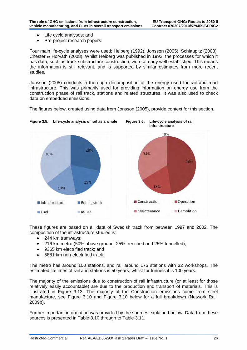
The role of GHG emissions from infrastructure construction, EU Transport GHG: Routes to 2050 II vehicle manufacturing, and ELVs in overall transport emissions Contract 070307/2010/579469/SER/C2
Restricted-Commercial Ref. AEA/ED56293/Task 2 Paper Draft – Issue No. 1 26
Life cycle analyses; and
Pre-project research papers. Four main life-cycle analyses were used; Heiberg (1992), Jonsson (2005), Schlaupitz (2008), Chester & Horvath (2008). Whilst Heiberg was published in 1992, the processes for which it has data, such as track substructure construction, were already well established. This means the information is still relevant, and is supported by similar estimates from more recent studies. Jonsson (2005) conducts a thorough decomposition of the energy used for rail and road infrastructure. This was primarily used for providing information on energy use from the construction phase of rail track, stations and related structures. It was also used to check data on embedded emissions. The figures below, created using data from Jonsson (2005), provide context for this section.
Figure 3.5: Life-cycle analysis of rail as a whole
Figure 3.6: Life-cycle analysis of rail infrastructure
These figures are based on all data of Swedish track from between 1997 and 2002. The composition of the infrastructure studied is:
244 km tramways;
216 km metro (50% above ground, 25% trenched and 25% tunnelled);
9365 km electrified track; and
5881 km non-electrified track. The metro has around 100 stations, and rail around 175 stations with 32 workshops. The estimated lifetimes of rail and stations is 50 years, whilst for tunnels it is 100 years. The majority of the emissions due to construction of rail infrastructure (or at least for those relatively easily accountable) are due to the production and transport of materials. This is illustrated in Figure 3.13. The majority of the Construction emissions come from steel manufacture, see Figure 3.10 and Figure 3.10 below for a full breakdown (Network Rail, 2009b). Further important information was provided by the sources explained below. Data from these sources is presented in Table 3.10 through to Table 3.11.

EU Transport GHG: Routes to 2050 II The role of GHG emissions from infrastructure construction, Contract 070307/2010/579469/SER/C2 vehicle manufacturing, and ELVs in overall transport emissions
Restricted-Commercial Ref. AEA/ED56293/Task 2 Paper Draft – Issue No. 1 27
Schlaupitz (2008) provides high-end estimates for stations, tunnels and bridges in the context of new electrified rail infrastructure. Tunnel proportions and earthworks vary widely from route to route, depending on factors such topography and soil conditions. They assume that an average tunnel proportion of 37% is a reasonable average to use for new lines, in comparison to 10% used in the UK (Network Rail, 2009). A summary of the rail route assumptions used is provided below:
Figure 3.7: Schalupitz assumptions for cross-regional high speed track
Chester & Horvath (2008) look in detail at different station designs and calculate in-use emissions and more detailed categories such as station cleaning and maintenance energy requirements. This study was also used to provide a total figure on all rail infrastructure energy consumption for comparison with others. Five rail transit systems are considered: the San Francisco‟s Bay Area Rapid Transit System (BART), Municipal Railway (Muni), Caltrain, Boston‟s Green Line, and the proposed California High Speed Rail (CAHSR). The BART and Caltrain systems are considered Heavy Rail Transit (HRT) while the Muni and Green Line are considered Light Rail Transit (LRT). The CAHSR is a high speed heavy real system which is expected to compete with air modes in the Sacramento to San Diego corridor. Of these five systems, only Caltrain trains are powered directly by diesel fuel while the others are powered by electricity. These four systems encompass the short and long range distance heavy and light rail systems. Figures on different average station types for various networks are provided in the table below.
Figure3.8: Material requirements for various station types
Rail system Units BART Caltrain Muni Green Line CAHSR Mean
Concrete Million cubic feet 26.0 0.6 6.8 5.9 1.1 8.1
Ballast Million cubic feet - 0.3 - - 0.5 0.2
Steel Thousand lbs 810.0 18.0 210.0 180.0 32.0 250.0
The range can be seen more clearly below:

The role of GHG emissions from infrastructure construction, EU Transport GHG: Routes to 2050 II vehicle manufacturing, and ELVs in overall transport emissions Contract 070307/2010/579469/SER/C2
Restricted-Commercial Ref. AEA/ED56293/Task 2 Paper Draft – Issue No. 1 28
Figure 3.9: Material requirements for various station types
The five systems show vastly different infrastructure configurations because of the differences in vehicle types, passengers served, and geography covered. Pre-project research papers from Network Rail in the UK were used to provide an understanding of likely practices if rail infrastructure were developed today. This gave quantities of material needed for various components of rail infrastructure and their associated embedded emissions, as well as in-use water, heating and electricity energy consumption from stations. An AEA study for Network Rail (Network Rail, 2009b) compared the environmental impact of conventional and high speed rail. As part of this study, the energy consumption and emissions resulting from rail infrastructure were also identified. Estimates for the embedded emissions from new rail infrastructure in the study were developed based on material use, materials transport (construction materials and excavated soil) and energy used for boring tunnels. Illustrative breakdowns of the materials use and greenhouse net gas emissions are provided in Figure 3.10. The analyses show that tunnelling and bridges contribute significantly to the totals, and therefore the assumptions made associated with these are therefore very important. The results also show that the type of track laid has a significant impact on the total embedded emissions, in the order of 30-40 tonnes CO2 eq per rail track km. 75% of the total embedded GHG emissions (from less than 50% of the raw materials used in the construction) can be attributed to the use of concrete and steel. According to Network Rail (2009b), the most carbon intensive aspect of rail infrastructure is Overhead Line Equipment, driven by the high embedded emissions in steel production. A breakdown of all components is provided in the figure below, split by the type of supporting structure.
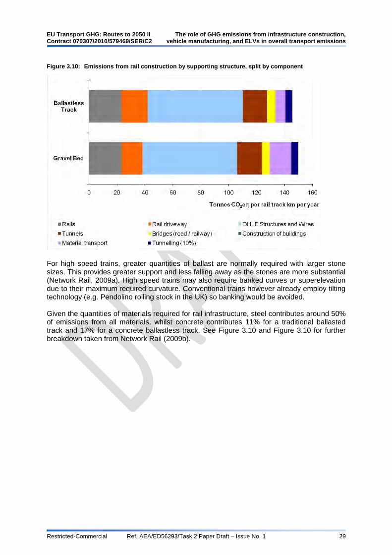
EU Transport GHG: Routes to 2050 II The role of GHG emissions from infrastructure construction, Contract 070307/2010/579469/SER/C2 vehicle manufacturing, and ELVs in overall transport emissions
Restricted-Commercial Ref. AEA/ED56293/Task 2 Paper Draft – Issue No. 1 29
Figure 3.10: Emissions from rail construction by supporting structure, split by component
For high speed trains, greater quantities of ballast are normally required with larger stone sizes. This provides greater support and less falling away as the stones are more substantial (Network Rail, 2009a). High speed trains may also require banked curves or superelevation due to their maximum required curvature. Conventional trains however already employ tilting technology (e.g. Pendolino rolling stock in the UK) so banking would be avoided. Given the quantities of materials required for rail infrastructure, steel contributes around 50% of emissions from all materials, whilst concrete contributes 11% for a traditional ballasted track and 17% for a concrete ballastless track. See Figure 3.10 and Figure 3.10 for further breakdown taken from Network Rail (2009b).

The role of GHG emissions from infrastructure construction, EU Transport GHG: Routes to 2050 II vehicle manufacturing, and ELVs in overall transport emissions Contract 070307/2010/579469/SER/C2
Restricted-Commercial Ref. AEA/ED56293/Task 2 Paper Draft – Issue No. 1 30
Figure 3.11: Material breakdown for conventional ballasted track
Total tonnes of material: 42,521
Figure 3.12: Material breakdown for ballastless track
Total tonnes of material: 38,174
Figure 3.13: Breakdown of embedded greenhouse gas emissions of conventional ballasted track, for production and disposal based on 50% recycling rate
Tonnes of CO2 per rail track km per year: 150
Figure 3.14: Breakdown of embedded greenhouse gas emissions for ballastless track, for production and disposal based on 50% recycling rate
Tonnes of CO2 per rail track km per year: 146
The embedded emissions resulting from the construction and eventual decommissioning of rail infrastructure are expected to be very significant primarily due to the very large quantities of steel and concrete used, which are both highly energy intensive in their production. Steel manufacture is highly intensive because of the reduction process which involves temperatures of around 1600OC. This can lead to considerable indirect emissions from power generation depending on the fuel source used to supply the energy.

EU Transport GHG: Routes to 2050 II The role of GHG emissions from infrastructure construction, Contract 070307/2010/579469/SER/C2 vehicle manufacturing, and ELVs in overall transport emissions
Restricted-Commercial Ref. AEA/ED56293/Task 2 Paper Draft – Issue No. 1 31
Concrete is a combination of cement and aggregate. Cement, like steel, is energy intensive and requires temperatures of around 1450OC, which could lead to high indirect emissions. Further, the chemical process of calcination, where CO2 is liberated from calcium carbonate to form quicklime, adds to its emissions intensity. The overwhelmingly dominant track form worldwide is the conventional ballasted track, which consists of flat-bottom steel rails supported on timber or pre-stressed concrete sleepers with gravel ballast. Assumptions on the amount of tunnelling and bridging were taken from IJLCA (2003). Data which supports this information is provided in Table 3.6. A study for UIC (2009) developed a carbon footprint of High-Speed rail infrastructure. As part of this study, the energy used and emissions associated with infrastructure were analysed in the context of emissions from the operation of High-Speed rail, the construction of the rolling stock, and the construction of the infrastructure itself. Three scenarios were considered:
Scenario 1: Electricity mix with low carbon footprint, average share of tunnels and bridges, high traffic on rail network, high load factor.
Scenario 2: Electricity mix with high carbon footprint, average share of tunnels and bridges, high traffic on rail network, high load factor.
Scenario 3: Electricity mix with high carbon footprint, high share of tunnels and bridges, low traffic on rail network, low load factor.
The results of these studies are provided below, and give a range of results which adds to those presented above.
Table 3.3: Emissions of CO2 from rail lifecycle scenarios (UIC, 2009)
Scenario Operation Rolling Stock Track System
gCO2 % gCO2 % gCO2 %
1 3.75 61 0.49 8 1.95 31
2 19.62 89 0.50 2 1.95 9
3 10.44 13 1.47 2 66.59 85

The role of GHG emissions from infrastructure construction, EU Transport GHG: Routes to 2050 II vehicle manufacturing, and ELVs in overall transport emissions Contract 070307/2010/579469/SER/C2
Restricted-Commercial Ref. AEA/ED56293/Task 2 Paper Draft – Issue No. 1 32
Figure 3.15: Carbon footprint of High-Speed Rail – CO2 emissions for three scenarios (adapted from UIC, 2009)
Figure 3.16: Carbon footprint of High-Speed Rail – % of CO2 emissions for track system, rolling stock and operation for three scenarios (adapted from UIC, 2009)

EU Transport GHG: Routes to 2050 II The role of GHG emissions from infrastructure construction, Contract 070307/2010/579469/SER/C2 vehicle manufacturing, and ELVs in overall transport emissions
Restricted-Commercial Ref. AEA/ED56293/Task 2 Paper Draft – Issue No. 1 33
The study results demonstrated that the share of emissions attributed to rail infrastructure are not negligible, as scenarios 1 (31%) and scenario 3 (85%) showed. However, the specific share that is attributed to infrastructure depends on a range of different factors, including the electricity mix, the traffic on the rail network and the share of bridges and tunnels (UIC, 2009). Claro (2010) identifies the emissions associated with transport infrastructure, in particular road and rail, and makes a comparison between the two, taking into consideration the full life cycle emissions of each mode. The key emissions figures related to rail and rail infrastructure are presented below.
Table 3.4: Rail infrastructure life cycle emissions
Stage Total Emissions (kg CO2) Relative emissions (%)
Manufacture of materials 6,469,524 15.24
Construction 25,321,412 59.65
Operation 9,631,600 22.69
End of life 1,026,865 2.42
Total 42,449,402 100
Figure 3.17: Total CO2 emissions for rail infrastructire (kg CO2) (adapted from Claro, 2010)

The role of GHG emissions from infrastructure construction, EU Transport GHG: Routes to 2050 II vehicle manufacturing, and ELVs in overall transport emissions Contract 070307/2010/579469/SER/C2
Restricted-Commercial Ref. AEA/ED56293/Task 2 Paper Draft – Issue No. 1 34
Figure 3.18: Total CO2 emissions for rail infrastructure (%) (Adapted from Claro, 2010)
Comparing this to other studies, the proportion of emissions attributed to construction seems quite high, i.e. in comparison to those presented in the Jonsson (2005) study (59.65%, or 74.89% when including manufacture of materials, compared to 48%). However, it appears that maintenance of the rail infrastructure has not been factored into these figures. Further, the study by Jonsson (2005) includes metro and tram systems in its calculations which may require high maintenance per track km due to the frequency of such services and convoluted urban routings with many points and crossovers.
Table 3.5: Emissions for rail infrastructure (kg CO2)
Source Emissions (kg CO2) Emissions (%)
Infrastructure life cycle 42,449,402 87.56
Vehicle propulsion 0 0
Vehicle life cycle 5,283,090 10.90
Fuel life cycle 745,505 1.54
Total emissions 48,477,997 -
Emissions per passenger transported 1.77 -
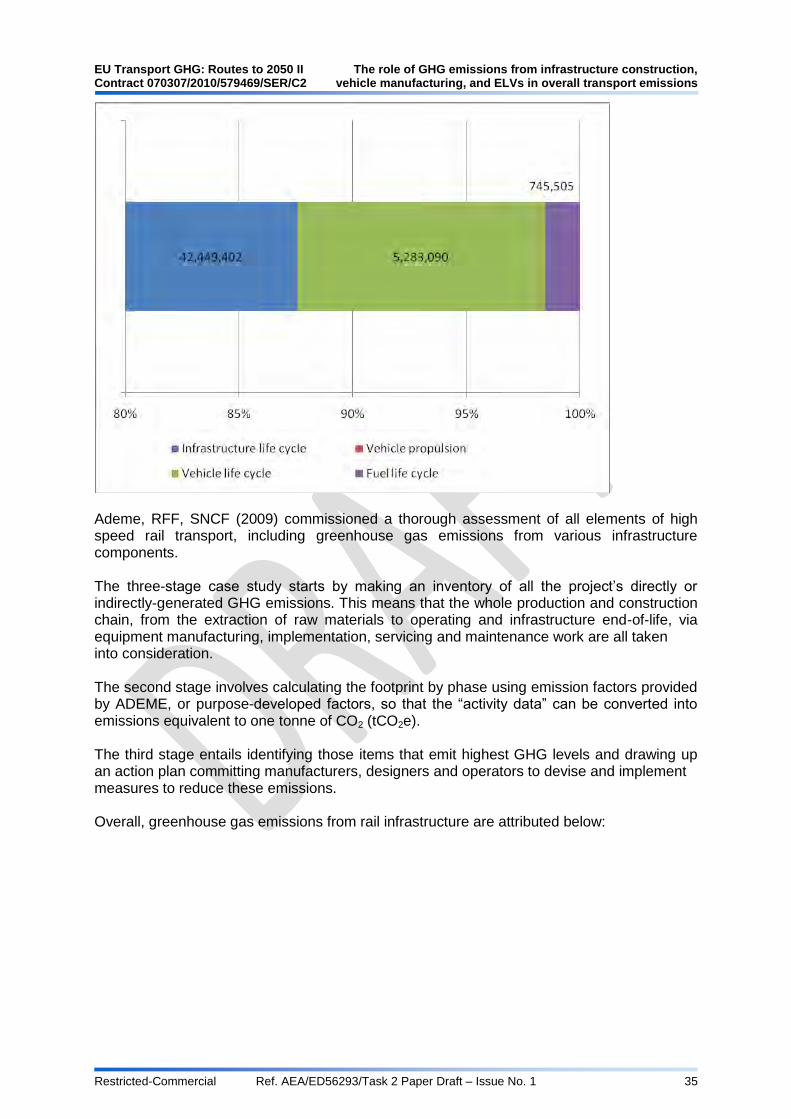
EU Transport GHG: Routes to 2050 II The role of GHG emissions from infrastructure construction, Contract 070307/2010/579469/SER/C2 vehicle manufacturing, and ELVs in overall transport emissions
Restricted-Commercial Ref. AEA/ED56293/Task 2 Paper Draft – Issue No. 1 35
Ademe, RFF, SNCF (2009) commissioned a thorough assessment of all elements of high speed rail transport, including greenhouse gas emissions from various infrastructure components. The three-stage case study starts by making an inventory of all the project‟s directly or indirectly-generated GHG emissions. This means that the whole production and construction chain, from the extraction of raw materials to operating and infrastructure end-of-life, via equipment manufacturing, implementation, servicing and maintenance work are all taken into consideration. The second stage involves calculating the footprint by phase using emission factors provided by ADEME, or purpose-developed factors, so that the “activity data” can be converted into emissions equivalent to one tonne of CO2 (tCO2e). The third stage entails identifying those items that emit highest GHG levels and drawing up an action plan committing manufacturers, designers and operators to devise and implement measures to reduce these emissions. Overall, greenhouse gas emissions from rail infrastructure are attributed below:

The role of GHG emissions from infrastructure construction, EU Transport GHG: Routes to 2050 II vehicle manufacturing, and ELVs in overall transport emissions Contract 070307/2010/579469/SER/C2
Restricted-Commercial Ref. AEA/ED56293/Task 2 Paper Draft – Issue No. 1 36
Figure 3.19: Overview of greenhouse gas emissions from rail infrastructure
Civil engineering works comprise the largest proportion of the construction phase rail infrastructure. This is broken down into the components shown below.
Figure 3.20: Greenhouse gas emissions from rail infrastructure civil engineering works
Embedded emissions from input materials comprise nearly ¾ of total construction phase emissions, or 53% of total infrastructure construction emissions. Of railway equipment (11% of total) 91% of emissions are from tracks, catenaries and work bases. Full details of this study are provided below.

EU Transport GHG: Routes to 2050 II The role of GHG emissions from infrastructure construction, Contract 070307/2010/579469/SER/C2 vehicle manufacturing, and ELVs in overall transport emissions
Restricted-Commercial Ref. AEA/ED56293/Task 2 Paper Draft – Issue No. 1 37
Figure 3.21: Rail infrastructure construction phase: Ademe, RFF, SNCF (2009) data
Construction phase Component tCO2eq
Civil engineering works Accumulated depreciation:
2,750
Ancillary work:
9,200
Input materials:
550,000
Internal energy of specific LGV buildings
1,100
Materials excavation and placement (internal processes):
41,000
Personnel transport:
47,300
Transport of materials by lorry (freight):
107,400
Connections to the existing rail network Connections to the existing rail network
55,000
Construction of TGV train sets
Construction of TGV train sets
95,000
Railway equipment SEI/CAI technical buildings:
730
Signalling equipment and hot box detector (SEI DBC):
2,200
Signalling, energy, cable routes:
5,500
Telecommunications :
730
Tracks, catenaries, work bases:
106,300
Traction supply:
1,100
Stations and other railway buildings Alteration work to existing stations
1,800
Alterations to the Technicentres:
4,000
Construction of maintenance bases:
4,500
Construction of two TGV stations:
20,000
Grand Total
1,055,610
Alternatives to reduce greenhouse gas emissions Kato et al (2005) conduct a lifecycle assessment of MAGLEV, including its infrastructure. The idea of the study is to look at the possibility that MAGLEV could compete with Shinkansen or Air travel in Japan‟s future transport strategy. A summary of the emissions from infrastructure are provided below:

The role of GHG emissions from infrastructure construction, EU Transport GHG: Routes to 2050 II vehicle manufacturing, and ELVs in overall transport emissions Contract 070307/2010/579469/SER/C2
Restricted-Commercial Ref. AEA/ED56293/Task 2 Paper Draft – Issue No. 1 38
Figure 3.22: MAGLEV construction, maintenance and repair CO2 emissions
Maintenance and repair of various components are a fraction of the emissions of the initial construction, 4% on average. This is confirmed by RTRI (2002) who state that the maintenance phase accounts for 3 to 7 % of that at the construction phase. Maglev does not however offer overall carbon savings compared to conventional high speed trains however, according to the life-cycle study of a Tokyo – Osaka route by Kato et al (2005). Lifecycle emissions per passenger kilometre are lower compared with air travel, but higher compared with Shinkansen.
Figure 3.23: Comparison of lifecycle emissions for Osaka – Tokyo route, Kato et al (2005)

EU Transport GHG: Routes to 2050 II The role of GHG emissions from infrastructure construction, Contract 070307/2010/579469/SER/C2 vehicle manufacturing, and ELVs in overall transport emissions
Restricted-Commercial Ref. AEA/ED56293/Task 2 Paper Draft – Issue No. 1 39
3.2.2 Development of emissions factors for the analysis
Data on infrastructure construction emissions factors
Table 3.6: Rail infrastructure embedded emissions from components and materials
Embedded Emissions Material Tonnes of material needed per track km
kgCO2 / tonne material
Average Lifetime
Units Medium Value
Stations Concrete 0.7 176.0 100 kgCO2 / track km
114
Bricks 1.3 192.0 100 kgCO2 / track km
250
Rail Steel 282.0 3,100.0 30 kgCO2 / track km
874,200
Ballast Gravel 7,950.0 8.0 15 kgCO2 / track km
63,600
Concrete 990.0 176.0 30 kgCO2 / track km
174,240
Ballastless track Concrete 4,500.0 176.0 60 kgCO2 / track km
792,000
Steel 132.0 3,100.0 60 kgCO2 / track km
409,200
Tunnel Soil 27,000.0 4.0 100 kgCO2 / track km
108,000
Concrete 4,400.0 176.0 kgCO2 / track km
774,400
Steel 210.0 3,100.0 kgCO2 / track km
651,000
Bridge Concrete 890.0 176.0 50 kgCO2 / track km
156,640
Steel 49.0 3,100.0 kgCO2 / track km
151,900
Retained cut Concrete 176.0 kgCO2 / track km
-
Road crossings and culverts
Concrete 176.0 kgCO2 / track km
-
Distance and curves kgCO2 / track km
-
Overhead Line Equipment Steel 500.0 3,100.0 30 kgCO2 / track km
1,550,000
Aluminium 70.5 11,000.0 30 kgCO2 / track km
775,086
Copper 138.1 1,701.0 30 kgCO2 / track km
234,919
Electrified third rail Steel 141.0 3,100.0 kgCO2 / track km
437,100
Insulator -
Points Steel GJ / track km
237
Data on construction energy consumption
Other than building a station which incorporates rail, road, metro rail and air travel, tunnelling has the highest potential for energy consumption in the construction phase. This is heavily influenced by the geology of the land being tunnelled; hard rock is energy intensive to mine and also time consuming. Bridges also have a high potential for energy consumption requirements, particularly if built over water and at great heights.

The role of GHG emissions from infrastructure construction, EU Transport GHG: Routes to 2050 II vehicle manufacturing, and ELVs in overall transport emissions Contract 070307/2010/579469/SER/C2
Restricted-Commercial Ref. AEA/ED56293/Task 2 Paper Draft – Issue No. 1 40
Table 3.7: Rail infrastructure construction energy consumption
Construction
Units Construction period
Energy Low Medium High
Low High Units
Stations Total - 5.0 GJ / track km / single track
784 3,761 42,409
Track Substructure (including embedded emissions)
GJ / track km / single track
2,161 4,642 9,436
Track Base (Including embedded emissions)
GJ / track km / single track
5,150 6,300 6,779
Track Substructure (excluding embedded emissions)
GJ / track km / single track
3,085
Blasting GJ / track km / single track
1,300
Movement of earth, stones, incl. Drilling
GJ / track km / single track
1,785
Track Base (excluding embedded emissions)
GJ / track km / single track
1,341
Welding GJ / track km / single track
9
Rail Fastening GJ / track km / single track
575
Installation GJ / track km / single track
757
Tunnel GJ / track km / single track
1,169 4,365 17,429
Bridge Years / track km
0.5 2.5 GJ / track km / single track
1,169 10,502
Materials for contact wires, transformers, signal system, stations, platforms, lighting, service roads
GJ / track km / single track
9,168
Material transport Litres of diesel
3
Data on construction emissions
For some of the elements above, readily converted information has been obtained for greenhouse gas emissions. This is presented in the table below.
Table 3.8: Rail infrastructure construction emissions
Construction
Emissions Medium value
Notes Units
Tunnel tCO2e / track km
5.0 10% of route assumed to be tunnelled, emission factor of 0.411 used
Bridge 1% of route assumed to be bridged
Material transport kgCO2 / 100 tonne km
8.4
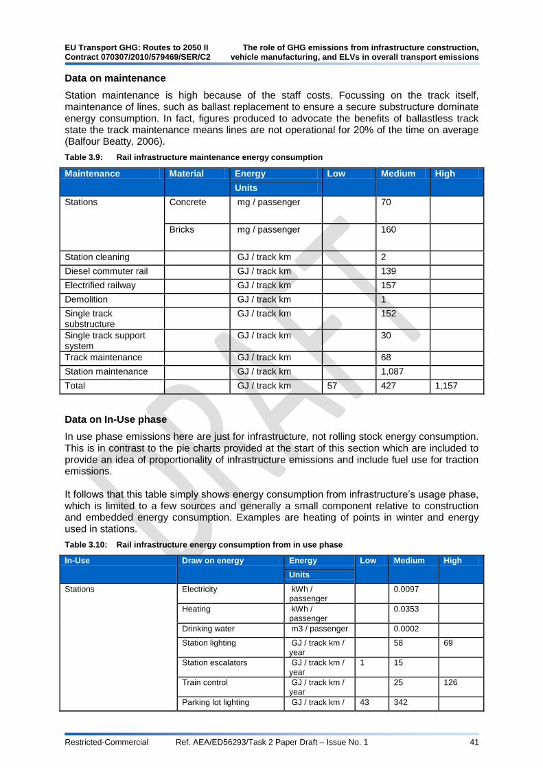
EU Transport GHG: Routes to 2050 II The role of GHG emissions from infrastructure construction, Contract 070307/2010/579469/SER/C2 vehicle manufacturing, and ELVs in overall transport emissions
Restricted-Commercial Ref. AEA/ED56293/Task 2 Paper Draft – Issue No. 1 41
Data on maintenance
Station maintenance is high because of the staff costs. Focussing on the track itself, maintenance of lines, such as ballast replacement to ensure a secure substructure dominate energy consumption. In fact, figures produced to advocate the benefits of ballastless track state the track maintenance means lines are not operational for 20% of the time on average (Balfour Beatty, 2006).
Table 3.9: Rail infrastructure maintenance energy consumption
Maintenance Material Energy Low Medium High
Units
Stations Concrete mg / passenger 70
Bricks mg / passenger 160
Station cleaning GJ / track km 2
Diesel commuter rail GJ / track km 139
Electrified railway GJ / track km 157
Demolition GJ / track km 1
Single track substructure
GJ / track km 152
Single track support system
GJ / track km 30
Track maintenance GJ / track km 68
Station maintenance GJ / track km 1,087
Total GJ / track km 57 427 1,157
Data on In-Use phase
In use phase emissions here are just for infrastructure, not rolling stock energy consumption. This is in contrast to the pie charts provided at the start of this section which are included to provide an idea of proportionality of infrastructure emissions and include fuel use for traction emissions. It follows that this table simply shows energy consumption from infrastructure‟s usage phase, which is limited to a few sources and generally a small component relative to construction and embedded energy consumption. Examples are heating of points in winter and energy used in stations.
Table 3.10: Rail infrastructure energy consumption from in use phase
In-Use Draw on energy Energy Low Medium High
Units
Stations Electricity kWh / passenger
0.0097
Heating kWh / passenger
0.0353
Drinking water m3 / passenger 0.0002
Station lighting GJ / track km / year
58 69
Station escalators GJ / track km / year
1 15
Train control GJ / track km / year
25 126
Parking lot lighting GJ / track km / 43 342
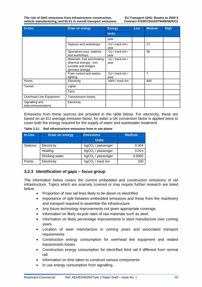
The role of GHG emissions from infrastructure construction, EU Transport GHG: Routes to 2050 II vehicle manufacturing, and ELVs in overall transport emissions Contract 070307/2010/579469/SER/C2
Restricted-Commercial Ref. AEA/ED56293/Task 2 Paper Draft – Issue No. 1 42
In-Use Draw on energy Energy Low Medium High
Units
year
Stations and workshops GJ / track km / year
27
Operations excl. stations and workshops
GJ / track km / year
86
Materials, fuel and heating (thermal energy) , incl. tunnells and bridges (primary energy)
GJ / track km / year
-
Train control and station lighting
GJ / track km / year
7
Points Electricity kWh / track km 840
Tunnel Lights
Fans
Overhead Line Equipment Transmission losses
Signalling and telecommunications
Electricity
Emissions from these sources are provided in the table below. For electricity, these are based on an EU average emission factor, for water a UK conversion factor is applied twice to cover both the energy required for the supply of water and wastewater treatment.
Table 3.11: Rail infrastructure emissions from in use phase
In-Use Draw on energy Emissions Medium
Units
Stations Electricity kgCO2 / passenger 0.004
Heating kgCO2 / passenger 0.014
Drinking water kgCO2 / passenger 0.0002
Points Electricity kgCO2 / track km 330
3.2.3 Identification of gaps – focus group
The information below covers the current embedded and construction emissions of rail infrastructure. Topics which are scarcely covered or may require further research are listed below:
Proportion of new rail lines likely to be diesel vs electrified
Importance of split between embedded emissions and those from the machinery
and transport required to assemble the infrastructure.
Any future technology improvements not given appropriate coverage.
Information on likely recycle rates of raw materials such as steel.
Information on likely percentage improvements in steel manufacture over coming
years.
Location of steel manufacture in coming years and associated transport
requirements.
Construction energy consumption for overhead line equipment and related
transmission losses
Construction energy consumption for electrified third rail if different from normal
rail.
Information on time taken to construct various components.
In use energy consumption from signalling.

EU Transport GHG: Routes to 2050 II The role of GHG emissions from infrastructure construction, Contract 070307/2010/579469/SER/C2 vehicle manufacturing, and ELVs in overall transport emissions
Restricted-Commercial Ref. AEA/ED56293/Task 2 Paper Draft – Issue No. 1 43
3.2.4 References
Balfour Beatty Rail Technologies, 2007, Embedded rail track system presentation. Available at: http://www.rfg.org.uk/files/CharlesPenny.pdf Chester, M., Horvath, A.,(2008) Environmental Life-cycle Assessment of Passenger Transportation: A Detailed Methodology for Energy, Greenhouse Gas and Criteria Pollutant Inventories of Automobiles, Buses, Light Rail, Heavy Rail and Air v.2 , University of California, Berkely. Available at: http://escholarship.org/uc/item/5670921q Claro, E (2010) Towards low-carbon transportation infrastructures, FAL Bulletin, Issue no. 286, no. 06, 2010. http://www.eclac.org/Transporte/noticias/bolfall/5/42195/FAL-286-WEB-ENG.pdf Dinha, VN., Kima, KD, Warnitchai, P (2009) Dynamic analysis of three-dimensional bridge–high-speed train interactions using a wheel–rail contact model. Available at: http://www.sciencedirect.com/science?_ob=ArticleURL&_udi=B6V2Y-4X5BP0K-1&_user=525224&_coverDate=12%2F31%2F2009&_alid=1698306829&_rdoc=2&_fmt=high&_orig=search&_origin=search&_zone=rslt_list_item&_cdi=5715&_sort=r&_st=13&_docanchor=&view=c&_ct=8571&_acct=C000026390&_version=1&_urlVersion=0&_userid=525224&md5=82d72614d0198fc9dade0fc885e6b088&searchtype=a#sec4 Discover Hong Kong (2011) Hong Kong Tourism Board description of Tsing Ma Bridge, http://www.discoverhongkong.com/eng/attractions/nt-tsingma-bridge.html, Last accessed 15/4/2011 EIR (2007) Bering Strait Tunnel, Alaska-Canada Rail. Infrastructure Corridors Will Transform Economy, by Richard Freeman and Dr. Hal Cooper, EIR (Executive Intelligence Review) Economics, 21 September 2007. Available at: http://www.larouchepub.com/eiw/public/2007/2007_30-39/2007-38/pdf/26-31_737.pdf Heiberg, E, (1992) Indirekte energibruk i persontransport, VF-rapport 20/92 IJLCA (2003) Ecology Profile of the German High-speed Rail Passenger Transport System, ICE, by Christian von Rozycki and Heinz Koeser (Martin-Luther-University, Germany) and Henning Schwarz (Deutsche Bahn AG, Germany). An LCA Case Study published in the International Journal of LCA 8 (2) 83 - 91 (2003). Jonsson, D. K., (2005) Indirekt energi för svenska väg- og järnvägtransporter, Totalförsvarets Forskningsinstitut, isbn 1650-1942. Available at: http://www.infra.kth.se/fms/pdf/FOI-R--1557--SE_v.2.pdf Lin, P.H, Tserng, H.P, Lin, C.C, (2005) Automated construction of the Paghuashan tunnel for Taiwan High Speed Rail (THSR) project. Available at: http://www.sciencedirect.com/science?_ob=MImg&_imagekey=B6V20-4HHP3GP-1-19&_cdi=5688&_user=525224&_pii=S0926580505001238&_origin=search&_coverDate=0%2F30%2F2006&_sk=999849994&view=c&wchp=dGLzVzz-zSkzk&md5=40582fba9325f7dceeb87194b1a9be5b&ie=/sdarticle.pdf Network Rail (2009a) Strategic Business Case. Available at: http://www.networkrail.co.uk/documents/About%20us/New%20Lines%20Programme/5883_Strategic%20Business%20Case.pdf Network Rail (2009b) Comparing environmental impact of conventional and high speed rail. Available at:

The role of GHG emissions from infrastructure construction, EU Transport GHG: Routes to 2050 II vehicle manufacturing, and ELVs in overall transport emissions Contract 070307/2010/579469/SER/C2
Restricted-Commercial Ref. AEA/ED56293/Task 2 Paper Draft – Issue No. 1 44
http://www.networkrail.co.uk/documents/About%20us/New%20Lines%20Programme/5878_Comparing%20environmental%20impact%20of%20conventional%20and%20high%20speed%20rail.pdf Rail Fan Europe (2011) Rail Fan Europe, Eurostar page. http://www.railfaneurope.net/tgv/eurostar.html. Last accessed 15/5/2011 Rail Safety and Standards Board UK (2009) Driver advisory information for energy management and regulation. Available at: http://www.rssb.co.uk/SiteCollectionDocuments/pdf/reports/research/T724_stage1_rpt_final.pdf RRA (2010) Position paper on track gauge, Railroad Association of South Africa. http://www.rra.co.za/?p=16022. Last accessed 15/4/2011, Schlaupitz, H., (2008) Energi- og klimakonsekvenser av moderne transportsystemer, Norsk Naturvernforbund Rapport 3/2008. Available at: http://naturvernforbundet.no/getfile.php/Dokumenter/rapporter/2008-2007/Energi%20og%20klimakonsekvenser%20av%20moderne%20transportsystemer.pdf Simonsen (2010) Transport, energi og miljø, Western Norway Research Institute. UIC (2009) Carbon footprint of High-Speed railway infrastructure: Methodology and application of High Speed railway operation of European Railways. UIC, France. http://uic.asso.fr/IMG/pdf/carbon_footprint_of_high_speed_rail_infrastructure_pre-study.pdf WF-Ingbau (2011) Wayss & Freytag Ingenieubau Company Home Site http://www.wf-ingbau.de/en/responsibilities/tunnelling/retained-cuts.html. Last accessed 15/4/2011
3.3 Aviation
3.3.1 Summary of information from the literature
Aviation infrastructure consists primarily of airport terminals, runways/tarmacs and ground support equipment (GSE). These aspects of aviation infrastructure are found at airport sites but their use depends on both the size and function of the airport. Aviation infrastructures are complex and different infrastructure systems are generally owned or operated by different organisations or companies, resulting in different impacts on energy and GHG emissions.
The Intergovernmental Panel on Climate Change (IPCC) estimated in 1999 that there was 12% inefficiency in air transport infrastructure. Since then, the International Air Transport Association (IATA) estimated that 4% efficiencies have been achieved in aviation infrastructure but there is still scope for significant improvement (IATA, 2009).
In 2008, IATA‟s work with industry partners resulted in 214 en route and 103 airport domain improvements for annual fuel savings that equated to 4 million tonnes of CO2. Using a Continuous Descent Arrival (CDA) rather than the traditional stepped approach to landing can save up to 630 kg of CO2 per landing. The number of airports by passenger carried in the EU27, EU15 and EU12 in 2010 is shown in Table 3.12. The CDA Action Plan initiated by IATA and other partners is estimated to save 500,000 tonnes of CO2 through implementing CDA at 100 airports across Europe by the end of 2013 (IATA, 2009).

EU Transport GHG: Routes to 2050 II The role of GHG emissions from infrastructure construction, Contract 070307/2010/579469/SER/C2 vehicle manufacturing, and ELVs in overall transport emissions
Restricted-Commercial Ref. AEA/ED56293/Task 2 Paper Draft – Issue No. 1 45
Table 3.12 EU Number of Airport by number of passengers carried per year (2010) (EU, 2010)
More than 10 million
5 to 10 million
1 to 5 million
500,000 to 1
million
100,000 to 500,000
15,000 to 100,000
TOTAL
EU27 30 31 94 39 116 90 400
EU15 29 27 78 35 106 81 356
EU12 1 4 16 4 10 9 44
Source: Eurostat, national sources
Accordingly to latest Eurostat figures, in 2009, more than 10% of the intra-EU transport took place between Spain and the United Kingdom (Eurostat, 2011a). Eight out of the top ten country pairs in terms of aviation passenger flow were either to or from Spain or the UK, as shown in Table 3.13. The influence of the economic crisis on the share in total international intra-EU transport of these top country-to-country flows was relatively limited according to the European Environment Agency (EEA).
Table 3.13: Top Intra-EU country pairs by passengers carried in 2009 (Eurostat, 2011b)
Rank Country Pairs Passengers carried (in
1000)
Share in total intra-
EU
1 Spain United Kingdom 30,551 10.1%
2 Germany Spain 20,391 6.7%
3 France United Kingdom 10,965 3.6%
4 Ireland United Kingdom 10,914 3.6%
5 Germany United Kingdom 10,709 3.5%
6 Germany Italy 10,414 3.4%
7 Italy United Kingdom 9,936 3.3%
8 Spain Italy 9,695 3.2%
9 Italy France 7,893 2.6%
10 France Spain 7,608 2.5%
The construction of terminals at airports contributes to the lifecycle GHG emissions of the aviation sector. Terminal construction can be likened to office buildings and shopping centres. The types of flights and airlines served at an airport will determine many of the design features of a terminal, including airport-wide services, baggage handling, areas for loading and unloading passengers and cargo, gate design and retail spaces. The top airports in the EU-27 in terms of passenger and freight carried in 2009 are shown in Table 3.14.
Table 3.14: Top airports in the EU-27 in terms of total passengers carried in 2009 (Eurostat, 2011c)
Rank Country Airport Total air transport (in 1000 passengers)
Total number of passenger
flights (in 1000)
1 UK London Heathrow 65,904 458
2 FR Paris Charles De Gaulle 57,689 497
3 DE Frankfurt Main 50,573 434
4 ES Madrid Barajas 47,944 418
5 NL Amsterdam Schiphol 43,532 383

The role of GHG emissions from infrastructure construction, EU Transport GHG: Routes to 2050 II vehicle manufacturing, and ELVs in overall transport emissions Contract 070307/2010/579469/SER/C2
Restricted-Commercial Ref. AEA/ED56293/Task 2 Paper Draft – Issue No. 1 46
Table 3.15: Top airports in the EU-27 in terms of total freight and mail carried in 2009 (Eurostat, 2011c)
Rank Country Airport Total air transport (in tons of freight/mail)
Total number of freight flights (in
1000)
1 DE Frankfurt Main 1,882,662 21
2 UK London Heathrow 1,348,914 3
3 NL Amsterdam Schiphol 1,316,848 13
4 FR Paris Charles De Gaulle
1,202,300 44
5 LU Luxembourg 627,261 10
The figures in Table 3.16 and Table 3.17 have been calculated from a UC Berkley study of lifecycle GHG emissions from aircrafts and their infrastructure (Eurostat 2011a; Eurostat, 2011b; Cester and Horvarth, 2007 & 2009). To evaluate airport impacts, the study took an average airport to make energy and GHG impacts. The top 50 US airports are responsible for 610 million of the 730 million passenger enplanements. From this, an average airport passenger enplanement of 12 million per year led Dulles Airport to be chosen as the median base line for calculations at an average airport. In all instances where ranges from this source are given, this represents the variation in impacts per vehicle type based on three typical aircrafts: Embraer 145, Boeing 737 and Boeing 747. GHG emissions from aviation infrastructure can come from the construction, operation or maintenance stages. When considering the construction of aviation infrastructure, the largest proportion of GHG emissions can be attributed to terminals, runways and tarmacs.
As shown in Table 3.16, the energy used to construct airport buildings is estimated at 549 MJ/ft2. Per aircraft-life, vehicle mile travelled and passenger mile travelled, the construction of airports uses 500-1,800 GJ, 37-210 kJ and 1.1kJ respectively (Chester and Horvarth, 2007).
When considering this construction process in terms of emissions, a range of 39-480 metric tonnes of GHG are accounted for per aircraft-life. 2.9-16g per vehicle mile and 0.089g per passenger mile travelled are the emissions calculated from the construction of airport terminals. As shown in Table 3.17, this equates to 43kg of GHG emissions for every ft2 constructed (Chester and Horvarth, 2007).
Quality and reliability characteristics influence the materials which are chosen to construct runways and the design specifications. The top 50 US airports average 3 to 4 runways which are all designed for the most demanding aircraft which will land at that airport (Chester and Horvarth, 2007).
The two primary materials commonly used to construct runways are concrete and asphalt. Asphalt has more flexibility making it less likely to crack under pressure but is not able to withstand as high temperatures as concrete. A combination of the two materials may be used at different parts of an airport based on the differences in their properties.
The energy associated with the construction of aviation infrastructure is dominated by the construction of runways and tarmacs. The energy intensive process of constructing a runway requires 136 MJ/ft2 of energy. Per vehicle mile travelled and per passenger mile travelled energy consumption associated with the runway construction process is 180-860 kJ and 4.7-5.7 kJ respectively (Chester and Horvarth, 2007).
When attributing emissions to the construction of runways, per aircraft-life emissions range from 180-2,100 metric tonnes whilst per-vehicle and per-mile emissions are 13-40g and 0.34-0.41g respectively. These calculations are based on a UC Berkley study which takes a range of life-cycle emissions from three aircrafts: Embraer 145, Boeing 737 and Boeing 747

EU Transport GHG: Routes to 2050 II The role of GHG emissions from infrastructure construction, Contract 070307/2010/579469/SER/C2 vehicle manufacturing, and ELVs in overall transport emissions
Restricted-Commercial Ref. AEA/ED56293/Task 2 Paper Draft – Issue No. 1 47
(Chester and Horvarth, 2007). When calculating the emissions associated with constructing a runway by area, an average of 10kg/ft2 is used.
In addition to the construction of terminals and runways at airports, taxiways and tarmacs are part of aviation infrastructures. Taxiways are the non-runway paths at an airport used by aircraft and tarmacs are considered the parking and staging areas near terminals, end of runways, and support facilities.
The construction of taxiways and tarmacs is estimated by UC Berkley to consume 6,400 – 77,000 GJ of energy per aircraft-life, 480-2,200 kJ of energy per vehicle-mile-travelled and 12-25 kJ of energy per passenger-mile-travelled (Eurostat, 2011b). These figures are based on a US study which uses the 6.1M ft2 of taxiway and 14M ft2 of tarmacs at Dulles airport as a typical airport which is then extrapolated. The ranges are dependent on the size and life-span of the aircraft, however this produces an estimated energy consumption for the construction of tarmacs of 95 MJ/ft2 (Eurostat, 2011a).
Table 3.16 : Energy Usage for Aviation Infrastructure Components (ranges of the parameters are given based on different aircraft sizes) (Adapted from Chester and Horvarth, 2009; 2007)
Life-Cycle Component Per Aircraft-life (GJ)
Per VMT (kJ)
Per PMT (kJ)
Per unit
Construction – Airports 500 – 1,800 GJ
37 – 210 kJ 1.1 kJ 549 MJ/ft2
Construction – Runways 2,500 – 30,000 GJ
180 – 860 kJ 4.7 – 5.7 kJ 136 MJ/ft2
Construction - Tarmacs 6,400 – 77,000 GJ
480 – 2,200 kJ
12 – 15 kJ 95 MJ/ft2
Infrastructure Operation – Runway lighting
1,200 – 3,400 GJ
86 – 400 kJ 2.2 – 2.7 kJ 471 GWH/yr*
Infrastructure Operation – Deicing Fluid Production
1,800 – 22,000 GJ
140 – 640 kJ 3.5 – 4.2 kJ 76 MJ/gal
Infrastructure Operation – Ground Support Equipment
15,000 – 170,000 GJ
1,100 – 5,100 kJ
28 – 34 kJ 47 MJ/LTO
Infrastructure Maintenance - Airports
25 – 310 GJ 1.8 – 10 kJ 0.057 kJ 28 MJ/ft2
* Total for all US airports
Table 3.17: Key GHG equivalent emissions from Aviation Infrastructure Components (ranges of the parameters are given based on different aircraft sizes) (adapted from Chester and Horvarth, 2009; 2007)
Life-Cycle Component Per Aircraft-life (Metric tonnes)
Per VMT (grams)
Per PMT (grams)
Per unit
Construction – Airports 39 – 480 2.9 – 16 g 0.089 g 43 kg/ft2
Construction – Runways 180 – 2,100 13 – 40 g
0.34 – 0.41 g
10 kg/ft2
Construction - Tarmacs 460 – 5,500 34 – 160 g 0.88 – 1.1 g 6.8 kg/ft2
Infrastructure Operation – Runway lighting
240 – 2,900 18 – 85 g 0.47 – 0.56 g
758 g/kWh
Infrastructure Operation – Deicing Fluid Production
140 – 1,600 10 – 47 g 0.26 – 0.31 g
6 kg/gal
Infrastructure Operation – Ground Support
1,100 – 13,000
82 – 390 g 2.1 – 2.6 g 4 kg/LTO

The role of GHG emissions from infrastructure construction, EU Transport GHG: Routes to 2050 II vehicle manufacturing, and ELVs in overall transport emissions Contract 070307/2010/579469/SER/C2
Restricted-Commercial Ref. AEA/ED56293/Task 2 Paper Draft – Issue No. 1 48
Life-Cycle Component Per Aircraft-life (Metric tonnes)
Per VMT (grams)
Per PMT (grams)
Per unit
Equipment
Infrastructure Maintenance - Airports
1.9 – 24 0.14 – 0.81 g 0.0045 g 2 mt/ft2
Following the construction of aviation infrastructure, there are significant emissions associated with the operational lifecycle of that equipment. The operation of runway lighting, terminal buildings, ground support equipment and the production of de-icing fluid are the largest contributors to these operational emissions from aviation infrastructure. The production of de-icing fluid for use at airports is a technology which produces GHG emissions. In the US, 35 million gallons of de-icing fluid are used each year during low temperatures (Chester and Horvarth, 2007). The large majority of airports use an ethylene or propylene glycol-based fluid. The fluid can impact water quality by reducing dissolved oxygen levels and therefore investment in appropriate precautions to manage this process is essential. Per aircraft-life (typically around 30 years), 1,800-22,000 GJ of energy and 140-1,600 metric tonnes of GHG emissions are produced as a result of de-icing fluid production technology. Per vehicle-mile-travelled this equates to 140-640 kJ or energy and 10-47g of emissions whist for passenger-miles travelled, 3.5-4.2 kJ and 0.26-0.31g of energy and emissions are associated respectively. There are case studies of where de-icing fluid can be recycled to reduce primary consumption, save energy and reduce GHG emissions. Munich Airport in Germany produces between 60-70% of its annual de-icing fluid requirements through recycling. Aircraft are de-iced on specially designated, remote areas at the airport, which are provided with a recovery system for de-icing fluids. Sprayed fluids are then stored before being trucked to a recycling facility, refined and distilled, enabling the glycol-based de-icing agent to be recovered. The process in Munich also generates „waste heat‟ as a by-product which covers a substantial share of the airport's heating requirements (ACI, 2008). Similar de-icing recovery takes place at Hamburg Airport, Germany and Zurich Airport, Switzerland. Per gallon, the production of de-icing fluid consumes 76 MJ of energy and produces 6kg of GHG emissions. From the US alone, the 35 million gallons of de-icing fluid produced annually therefore produces around 210 million kg of GHG emissions (ACI, 2008).
Runway lighting typically consists of four different types of systems; approach systems, centreline lights, touchdown lights and edge lights. The lighting systems are a necessary part of the aviation infrastructure but their use will vary seasonally and according to the daily hours of darkness of the runway location.
A US study of runway lighting inventoried the electricity consumption of airport lighting systems in 2002 (EERE, 2002). It estimated that the approach, centreline, touchdown and edge light systems consume 57, 120, 160, and 140 GWh annually across all U.S airports (EERE, 2002).
A UC Berkley study estimates that the energy consumption associated with the operation of runway lighting infrastructure is 1,200 – 3,400 GJ per aircraft-life, 86 – 400 kJ per vehicle-mile-travelled and 2.2 – 2.7 kJ per passenger-mile-travelled. Emissions from the construction of tarmacs/taxiways is lower than for runways per square foot (6.8 kg/ft2 compared to 10kg/ft2). However, per aircraft-life, vehicle-mile and passenger-mile travelled, the emissions are higher when constructing tarmacs compared to runways. Constructing tarmacs produces 460-5,500 metric tonnes of GHG emissions per aircraft-life, 34-160g per vehicle-mile-travelled and 0.88-1.1g per passenger-mile-travelled. These figures are based on a range of

EU Transport GHG: Routes to 2050 II The role of GHG emissions from infrastructure construction, Contract 070307/2010/579469/SER/C2 vehicle manufacturing, and ELVs in overall transport emissions
Restricted-Commercial Ref. AEA/ED56293/Task 2 Paper Draft – Issue No. 1 49
aircrafts at an airport in the US which has an average enplanement of 12 million passenger per year.
Ground Support Equipment used at airports uses significant amounts of energy and is mainly fuelled by either gasoline or diesel. The FAA estimated about 72,000 pieces of ground support equipment are in operation in the US alone. Although a comprehensive global inventory of GSE in operation does not exist, a study estimates that 30-40% operate on diesel fuel, 50-60% on gasoline and around 10% on alternative fuels.
The energy consumption and GHG emissions from the infrastructure operation of GSE can be estimated per aircraft-life, per vehicle mile travelled and per passenger mile travelled as shown in Table 3.16 and Table 3.17. When looking at energy consumption, the operation of GSE is attributed 15,000-170,000 GJ per aircraft life. This range is associated with the difference in both typical aircraft life and size, taking figures from three aircraft types: Embraer 145, Boeing 737 and Boeing 747. The range in energy consumption attributed to the operation of GSE per vehicle mile travelled is 1,100-5,100 kJ. Per passenger mile travelled, the energy consumption range is 28-34 kJ (Chester and Horvarth, 2007).
When looking at GHG emissions associated with the GSE infrastructure of aviation, per aircraft-life emissions range between 1,100-13,000 metric tonnes, depending on the type of aircraft and its typical lifespan. Per vehicle miles travelled emissions attributed to GSE operation is 82-390g whilst 2.1-2.6g of GHG emissions are attributed per passenger mile travelled. Per landing take-off cycle (LTO), 4 kg of GHG emissions are attributed to the operation of GSE infrastructure (Chester and Horvarth, 2007).
Table 3.18 Average Energy Consumption and Costs for GSE (adapted from ATAA, 1994; FFA and EPA, 1995;
24)
Energy consumption
(MJ per year) Conventional replacement
Electric replacement
Ground Support
Equipment
Economic Life
(years)
Use per year
(hours)
Diesel Gasoline Capital Cost US$
Maintenance Cost
Capital Cost US$
Maintenance Cost
GPU 8 2,240 2,177,229 2,955,113 $32,000 $10.44/hr - $7.83/hr
Van 8 1,987 - 1,046,574 $22,000 $10.09/hr - $10.09/hr
Pickup 8 1,722 - 906,996 $18,000 $9.65/hr $27,000 $7.24/hr
Aircraft Tug (Wide
Body) 10 1,721 6,152,726 8,072,619 $190,00 $26.41/hr $250,000 $19.71/hr
Bus 8 1,678 1,051,054 883,820 $110,000 $9.58/hr - $9.58/hr
Lift 8 1,357 - 795,653 $45,000 $13.73/hr $54,000 $10.30/hr
Cargo Loader
10 1,250 445,421 513,041 $150,000 $9.84/hr $180,000 $7.38/hr
Fuel Truck 8 1,117 699,659 588,336 $65,000 $16.83/hr - $16.83/hr
Air Start Unit
8 181 759,006 248,335 $80,000 £33.76/hr - $25.32/hr
According to a US study of four airports, seven ground access vehicles were the most significant source of mobile emissions, responsible for 45-68% of the airports‟ volatile organic compounds and 27-63% of the nitrogen oxides emitted from mobile sources (Energy and Environment Analysis, 1997)25.
24
Calculations of average operational fuel consumption calculated from [Error! Bookmark not defined.] (Load factor % x BHP x Gallons fuel per BHP/hour x Hourly use per year x MJ conversion ratio – 1 MJ = 0.007589 gallons gasoline or 0.006825 gallons diesel) 25
The four airports included in this study for the US EPA, were Baltimore-Washington International, Boston Logan International, Los Angeles International, and Phoenix Sky Harbor International.

The role of GHG emissions from infrastructure construction, EU Transport GHG: Routes to 2050 II vehicle manufacturing, and ELVs in overall transport emissions Contract 070307/2010/579469/SER/C2
Restricted-Commercial Ref. AEA/ED56293/Task 2 Paper Draft – Issue No. 1 50
Replacing GSE with alternative fuels, such as electricity, liquefied petroleum gas, and compressed natural gas could result in reduced greenhouse gas emissions. The energy use of GSE will also vary between diesel and gasoline options. Annually, an aircraft tug (for a wide body aircraft) is the piece of GSE which will typically consume the most energy. If diesel, the tug will consume 6,153 GJ whereas a gasoline alternative carrying out the same role will typically consume 31% more, 8,073 GJ (FFA and EPA, 1995). Data for other GSE which uses a large amount of energy are shown in Table 3.18. Ground Power Units are vehicles which supply power to an aircraft when it is on the ground. They can be a fixed source of power but will typically be remote to easily move between different aircrafts. In terms of ground support equipment, the GPU is the most used piece of equipment, typically being operational for 2,240 hours per year. The equipment has an economic life of 8 years and is typically either a diesel or gasoline vehicle. Annual operational energy consumption of GPUs varies depending on the vehicle fuel used; 2,177,229 MJ/year for diesel and 2,955,113 MJ/year for gasoline (FFA and EPA, 1995). Fixed gate power supply is an alternative aviation infrastructure technology to GPUs which supply aircrafts with power when they are on the ground. A fixed power supply can permit a reduction in the use of aircraft auxiliary power units and thereby reduce emissions. Airports are not required to install boarding gates that provide electricity to parked aircraft, but the Federation of Aviation Administration (FAA) report that some airports have been proactive in reducing emissions and have invested in these electric gates. The emissions attributable to the generation of electricity for fixed systems are going to be generated from an off-airport power source. These sources have greater control over emissions and a higher efficiency than on-board Alternative Power Units (APU). The EPA also acknowledges that the cost of the fuel saved is greater than the cost of electricity (FFA and EPA, 1995). When looking at the GHG emissions from infrastructure in the context of aircraft lifecycle emissions, the total emissions from infrastructure account for approximately 2.9% of lifecycle emissions from aviation. This is very small compared to the 78.6% of GHG emissions which come from the direct operation of aircrafts. This is outlined in more detail in Figure 3.24.
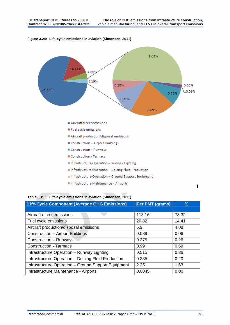
EU Transport GHG: Routes to 2050 II The role of GHG emissions from infrastructure construction, Contract 070307/2010/579469/SER/C2 vehicle manufacturing, and ELVs in overall transport emissions
Restricted-Commercial Ref. AEA/ED56293/Task 2 Paper Draft – Issue No. 1 51
Figure 3.24: Life-cycle emissions in aviation (Simonsen, 2011)
Table 3.19: Life-cycle emissions in aviation (Simonsen, 2011)
Life-Cycle Component (Average GHG Emissions) Per PMT (grams) %
Aircraft direct emissions 113.16 78.32
Fuel cycle emissions 20.82 14.41
Aircraft production/disposal emisisons 5.9 4.08
Construction – Airport Buildings 0.089 0.06
Construction – Runways 0.375 0.26
Construction - Tarmacs 0.99 0.69
Infrastructure Operation – Runway Lighting 0.515 0.36
Infrastructure Operation – Deicing Fluid Production 0.285 0.20
Infrastructure Operation – Ground Support Equipment 2.35 1.63
Infrastructure Maintenance - Airports 0.0045 0.00
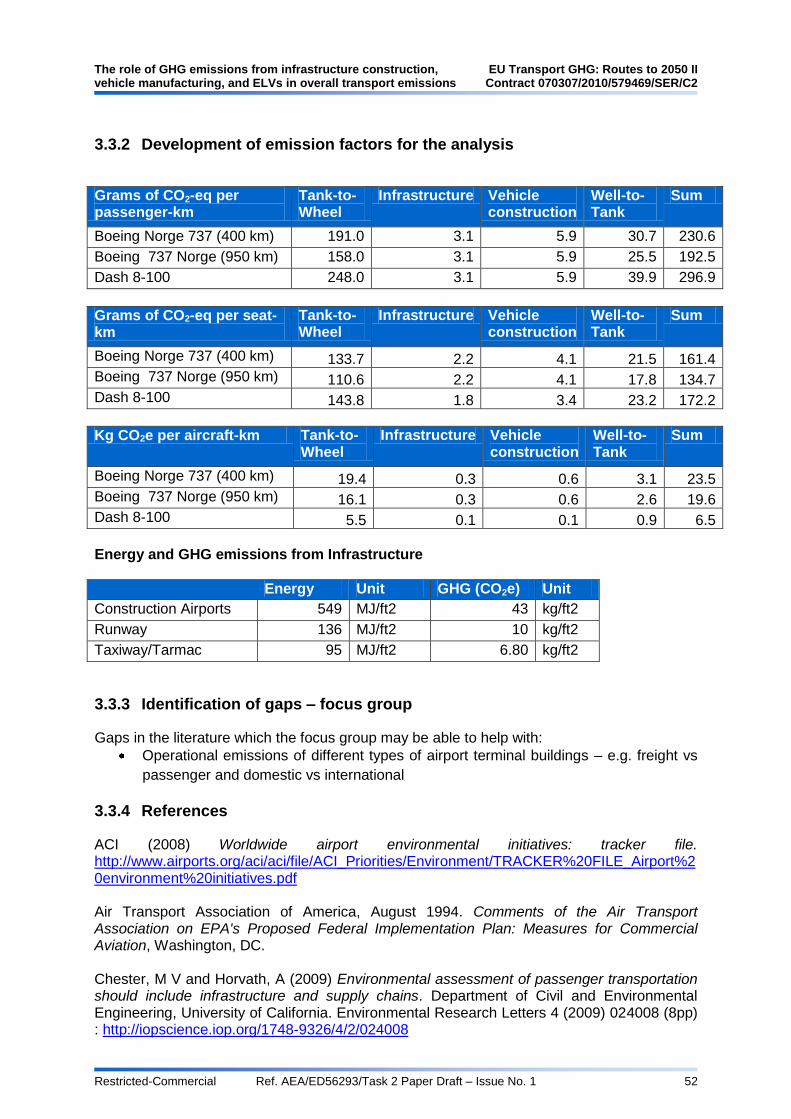
The role of GHG emissions from infrastructure construction, EU Transport GHG: Routes to 2050 II vehicle manufacturing, and ELVs in overall transport emissions Contract 070307/2010/579469/SER/C2
Restricted-Commercial Ref. AEA/ED56293/Task 2 Paper Draft – Issue No. 1 52
3.3.2 Development of emission factors for the analysis
Grams of CO2-eq per passenger-km
Tank-to-Wheel
Infrastructure Vehicle construction
Well-to-Tank
Sum
Boeing Norge 737 (400 km) 191.0 3.1 5.9 30.7 230.6
Boeing 737 Norge (950 km) 158.0 3.1 5.9 25.5 192.5
Dash 8-100 248.0 3.1 5.9 39.9 296.9
Grams of CO2-eq per seat-km
Tank-to-Wheel
Infrastructure Vehicle construction
Well-to-Tank
Sum
Boeing Norge 737 (400 km) 133.7 2.2 4.1 21.5 161.4
Boeing 737 Norge (950 km) 110.6 2.2 4.1 17.8 134.7
Dash 8-100 143.8 1.8 3.4 23.2 172.2
Kg CO2e per aircraft-km Tank-to-Wheel
Infrastructure Vehicle construction
Well-to-Tank
Sum
Boeing Norge 737 (400 km) 19.4 0.3 0.6 3.1 23.5
Boeing 737 Norge (950 km) 16.1 0.3 0.6 2.6 19.6
Dash 8-100 5.5 0.1 0.1 0.9 6.5
Energy and GHG emissions from Infrastructure
Energy Unit GHG (CO2e) Unit
Construction Airports 549 MJ/ft2 43 kg/ft2
Runway 136 MJ/ft2 10 kg/ft2
Taxiway/Tarmac 95 MJ/ft2 6.80 kg/ft2
3.3.3 Identification of gaps – focus group
Gaps in the literature which the focus group may be able to help with:
Operational emissions of different types of airport terminal buildings – e.g. freight vs
passenger and domestic vs international
3.3.4 References
ACI (2008) Worldwide airport environmental initiatives: tracker file. http://www.airports.org/aci/aci/file/ACI_Priorities/Environment/TRACKER%20FILE_Airport%20environment%20initiatives.pdf Air Transport Association of America, August 1994. Comments of the Air Transport Association on EPA's Proposed Federal Implementation Plan: Measures for Commercial Aviation, Washington, DC. Chester, M V and Horvath, A (2009) Environmental assessment of passenger transportation should include infrastructure and supply chains. Department of Civil and Environmental Engineering, University of California. Environmental Research Letters 4 (2009) 024008 (8pp) : http://iopscience.iop.org/1748-9326/4/2/024008

EU Transport GHG: Routes to 2050 II The role of GHG emissions from infrastructure construction, Contract 070307/2010/579469/SER/C2 vehicle manufacturing, and ELVs in overall transport emissions
Restricted-Commercial Ref. AEA/ED56293/Task 2 Paper Draft – Issue No. 1 53
Chester, M V and Horvath, A (2007). Environmental Life-cycle Assessment of Passenger Transportation: A Detailed Methodology for Energy, Greenhouse Gas and Criteria Pollutant Inventories of Automobiles, Buses, Light Rail, Heavy Rail and Air. UC Berkeley: UC Berkeley Center for Future Urban Transport. http://escholarship.org/uc/item/5bz4s1n3 EERE (2002) U.S. Lighting Market Characterization, Volume I: National Lighting Inventory and Energy Consumption Estimate, U.S. Department of Energy, Energy Efficiency and Renewable Energy, Prepared by Navigant Consulting, Inc., 9/2002 Energy and Environmental Analysis, Inc.,(1997) Analysis of Techniques to Reduce Air Emissions at Airports, (Arlington, VA: June 1997). EU (2010) EU energy and transport in figures: Statistical pocketbook 2010, European Union, Brussels. http://ec.europa.eu/transport/publications/statistics/statistics_en.htm Eurostat (2011a) Air transport statistics. http://epp.eurostat.ec.europa.eu/statistics_explained/index.php/Air_transport_statistics Eurostat (2011b) Intra-EU traffic at country level, Eurostat: http://epp.eurostat.ec.europa.eu/statistics_explained/index.php?title=File:Intra-EU_traffic_at_country_level_-_43_%25_of_the_2009_total_traffic_at_a_glance_(and_corresponding_2008_figures).PNG&filetimestamp=20110214144334 Eurostat (2011c) http://epp.eurostat.ec.europa.eu/statistics_explained/index.php?title=File:Top_airports_in_the_EU-27_in_terms_of_total_passengers_carried_in_2009.PNG&filetimestamp=20110214145415 FAA and EPA (1995) FAA and EPA‟s Technical Data to Support FAA’s Advisory Circular on Reducing Emissions from Commercial Aviation. Page 24-27: http://www.epa.gov/oms/regs/nonroad/aviation/faa-ac.pdf IATA (2009) A global approach to reducing aviation emissions: First stop: carbon-neutral growth from 2020. The International Air Transport Association November 2009: http://www.iata.org/SiteCollectionDocuments/Documents/Global_Approach_Reducing_Emissions_251109web.pdf Simonsen (2011) Transport, energi og Miljo: Dokumentasjonsside, http://vfp1.vestforsk.no/sip/index.html
3.4 Shipping
3.4.1 Summary of information from the literature
Port Infrastructure – An Overview
Ports provide essential connections between seaborne and land-based modes of transport. The main functions of a port are to supply services to freight (for example, storage or transhipment) and to vessels (refuelling, repairs etc). Maritime ports handle more freight than all of the other types of terminal combined (Rodrigue et al, 2009). Port facilities are determined by the type of cargo they must handle:

The role of GHG emissions from infrastructure construction, EU Transport GHG: Routes to 2050 II vehicle manufacturing, and ELVs in overall transport emissions Contract 070307/2010/579469/SER/C2
Restricted-Commercial Ref. AEA/ED56293/Task 2 Paper Draft – Issue No. 1 54
Liquid bulk cargoes, such as crude oil, are moved using pumps and pipelines; they require only limited handling equipment but may need significant storage capacity.
Dry bulk products are unpackaged goods such as ore, cereals and coal. Handling these materials requires more sophisticated equipment such as cranes, specialized grabs and conveyor belts. Some terminals have specialized storage structures such as grain silos and refrigerated warehouses.
General cargo requires a lot of labour to handle where dimensions and weights are not uniform. Containerisation of cargo has allowed handling to become mechanized and it is progressively more common for bulk products to be containerised.
Container terminals have minimal labour requirements, but generally require large amounts of space for moving and stacking containers.
Intermediate or transhipment ports are used for ship-to-ship operations. Their importance is growing, as they increase connectivity between global ports. Containers must be stored in the port temporarily, rather than being transferred directly.
The increase in containerised cargo was more than fivefold between 1990 and 2010 (UNCTAD, 2010). This has manifested a change in the configuration of port terminals, which have shifted from conventional bulk to containers since the 1960s. Generally, the larger the containerships handled by a port, the larger the required container storage area. The main elements required of a port include the docking areas for ships and refuelling infrastructure. Docking areas can be quite substantial in size, with typical 5,000-10,000 TEU post-PanaMax vessel ranging from 275-340m in length, 38-45m beam and 13-15m draught (Mayrick, 2007). Ships powered using alternative fuels such as nuclear power or hydrogen require ports that are able to store and handle these fuels. Ships can be docked for times ranging from one hour to three days. Shore-side power for ships while at dock, also known as cold-ironing, allows ships to turn off their diesel-powered auxiliary engines. A transformer is often needed for ships to be able to use shore-side electricity, and the local grid connection to the port must be upgraded. Another alternative is to use natural gas power generation. The Wittmar cold-ironing system can burn either compressed or liquefied natural gas (LNG). Infrastructure links, including rail and road, will also be of great significance when terms of port infrastructure, enabling the movement of freight to and from the ports (although dealt with under the rail and road sections above).
Construction of port infrastructure and GHG emissions
Whilst the range of infrastructure that makes up ports can be quite extensive, little literature currently exists that considers the embedded CO2 emissions associated with its production. This section considers studies where elements of port infrastructure have been considered in terms of embedded emissions or life cycle analysis. Luijten et al (2010) undertook research into the carbon footprint and CO2 emissions from port infrastructure at the Port of Rotterdam. The study considered two types of port infrastructure – road construction and quay wall construction. The individual components of these structures were categorised to assess each element of the contribution to the carbon footprint, which covered the whole process of design, construction and demolition. A number of quay wall types are used within the Port of Rotterdam. Three types of quay wall were selected for the study, which are:
Quay wall Antarticaweg – Sheetpile with concrete coping;
Quay wall Amazonehaven – Combi wall quay wall; and
Quay wall Euromax – Diaphragm quay wall with relieving floor.

EU Transport GHG: Routes to 2050 II The role of GHG emissions from infrastructure construction, Contract 070307/2010/579469/SER/C2 vehicle manufacturing, and ELVs in overall transport emissions
Restricted-Commercial Ref. AEA/ED56293/Task 2 Paper Draft – Issue No. 1 55
The key overview results of the carbon footprint for the quay wall types are shown in Figure 3.25.
Figure 3.25: Overview carbon footprint quay walls investigated (Luijten et al, 2010).
Figure 3.26 shows the CO2 emissions in more detail for the Antarticaweg quay wall. As the graph shows, CO2 emissions are dominated by the material component steel.
Figure 3.26: Carbon footprint for Antarticaweg quay wall in more detail (Luijten et al, 2010)
A Master thesis (Maas, 2011) also compares various quay wall designs with regards to CO2 emissions and LCA, including those made from concrete, steel, wood and composites. Emissions from the production of the materials, transportation and construction were all considered in the study. When comparing the carbon footprints of the four types of retaining walls, the wooden wall resulted in having the smallest carbon footprint, followed by steel and

The role of GHG emissions from infrastructure construction, EU Transport GHG: Routes to 2050 II vehicle manufacturing, and ELVs in overall transport emissions Contract 070307/2010/579469/SER/C2
Restricted-Commercial Ref. AEA/ED56293/Task 2 Paper Draft – Issue No. 1 56
concrete. The carbon footprint of the FRP panel is considerably larger. The CO2 emissions per 1 meter of each wall type were as follows:
Wood – 16 ton/kg CO2
Steel – 16.6 ton/kg CO2
Concrete – 20 ton/kg CO2
FRP – 115 ton/kg CO2.
Figure 3.27: CO2 emissions for 1m of quay wall (Maas, 2011)
Figure 3.28: CO2 emissions for 1m of quay retaining wall (Maas, 2011)
A study by Walnum (2011) considers both the direct and indirect emissions from cruise ships. The indirect emissions ideally considered would include the energy used and emissions produced during the construction, maintenance and operation of the cruise ship infrastructure, the harbours and the ship itself. The study uses the Ecoinvent database to determine such energy use and emissions. For example, a transoceanic tanker‟s life cycle CO2 emissions can be broken down as follows:
Operation of ship - 83%;
Port Operation – 15.07%;

EU Transport GHG: Routes to 2050 II The role of GHG emissions from infrastructure construction, Contract 070307/2010/579469/SER/C2 vehicle manufacturing, and ELVs in overall transport emissions
Restricted-Commercial Ref. AEA/ED56293/Task 2 Paper Draft – Issue No. 1 57
Ship Production – 2%;
Maintenance – 0.01; and
Construction of port facilities – 0.01%
Figure 3.29: Transoceanic lifecycle emissions of CO2 (adapted from Walnum 2011)
Other studies that were reviewed (Simonsen, 2010) also revealed that port infrastructure and the building of ships played a minor role in total lifecycle CO2 emissions. The combined total of emissions from these two processes varied from 2.7% for a Liquefied Natural Gas (LNG) tanker with a deadweight of 200,000 tonnes to 11.3% for a Liquefied Petroleum gas (LPG) tanker with a deadweight of 200,000 tonnes. For emissions from infrastructure alone, this ranged from >0.01% to 0.05% (see Table 4.16).

The role of GHG emissions from infrastructure construction, EU Transport GHG: Routes to 2050 II vehicle manufacturing, and ELVs in overall transport emissions Contract 070307/2010/579469/SER/C2
Restricted-Commercial Ref. AEA/ED56293/Task 2 Paper Draft – Issue No. 1 58
Figure 3.30: Ship production and construction of port infrastructure CO2 emissions as a percentage of total vessel lifecycle emissions (adapted from Walnum, 2011 and Simonsen 2010).
Port maintenance and operations and GHG emissions
A number of carbon footprint assessments have been undertaken of major ports using a methodology developed by the World Ports Climate Initiative (WPCI), which include an assessment of operational emissions. These assessments included the following emissions:
Direct emissions: Fuel usage for heating port buildings; by company owned cars; by operational vessels; and by operational machines and cranes.
Energy Indirect emissions: Electricity usage by cranes owned by port; for the purpose of harbour lighting; for buildings owned by port (e.g. heating, lighting); by lighthouses owned by port; and from other sources in port.
Other indirect emissions: car fuel usage by commuting employees (petrol and diesel); km driven by commuting employees (train, public transport, motorcycle, boat, walking and cycling), domestic business travel by plane, short-haul business travel by plane, long-haul business travel by train, business travel by taxi, business travel in non-company owned vehicles.
Available assessments include those for Oslo and Rotterdam, and a third has been undertaken for the Port of Jurong, partly using the WPCI methodology, but also drawing upon other carbon foot printing methodologies (so may not be directly comparable) (Ecofys, 2007; WPCC, 2008; Jurong Port Pte Ld, 2011). Figure 3.31 provides a detailed breakdown of CO2 emissions for the Port of Oslo for the year 2008. A large proportion of the CO2 emissions generated from port operations can be attributed to fuel for port vehicles (34% - direct emissions), electricity usage for buildings (20% - energy indirect emissions), commuting by car (17% - other indirect emissions), and harbour lighting (12% - energy indirect).

EU Transport GHG: Routes to 2050 II The role of GHG emissions from infrastructure construction, Contract 070307/2010/579469/SER/C2 vehicle manufacturing, and ELVs in overall transport emissions
Restricted-Commercial Ref. AEA/ED56293/Task 2 Paper Draft – Issue No. 1 59
Figure 3.31: Lifecycle emissions of CO2 for the Port of Oslo (Ecofys, 2007).
Table 3.20 and Figure 3.32 provide an overview of the life cycle CO2 emissions for the three ports. The differences in the methodologies used become evident here when considering the results of the LCA for Jurong Port. 88% of emissions are attributed to „other indirect emissions‟, mainly due to the inclusion of emissions from shipping vessels and tugboat operations. The proportion of „other indirect emissions‟ for Oslo and Rotterdam are 22% and 55% respectively, significantly lower. When these emissions are removed from the Jurong LCA, the proportion of „other indirect emissions‟ is reduced to 33%. Due to the differences between the ports considered in terms of size, location, port activity, cargo movements etc, it is expected that there will be variations in both the volume of emissions and proportion between types of emissions.
Table 3.20: Life cycle CO2 emissions of selected ports
Port Year Direct Emissions Energy Indirect Emissions
Other Indirect Emissions
No. % No. % No. %
Oslo 2008 594 44 463 34 289 22
Rotterdam 2007 8,960 25 7,230 20 20,100 55
Jurong* 2009 7,020 6 8,314 6 115,266 88
Jurong** 2009 7,020 31 8,314 36 7,426 33
*Other Indirect Emissions‟ in this LCA study includes shipping and tugboat operational emissions. ** Emissions for shipping and tugboat operations have been removed.

The role of GHG emissions from infrastructure construction, EU Transport GHG: Routes to 2050 II vehicle manufacturing, and ELVs in overall transport emissions Contract 070307/2010/579469/SER/C2
Restricted-Commercial Ref. AEA/ED56293/Task 2 Paper Draft – Issue No. 1 60
Figure 3.32: Life cycle emissions of selected ports
*’Other indirect emissions’ for this LCA includes shipping (vessels) and tugboats
No information was identified regarding the GHG emissions associated with maintenance operations that are carried out at ports. However, the Walnum (2011) study identified that the proportion of a tankers lifetime emissions attributed to maintenance were just 0.01%. Reducing future emissions from the construction, maintenance and operation of ports A Scandinavian consortium has developed a new process which blends contaminated sediment (extracted through dredging processes) with a special mix of binders. The resulting product is a safe construction material that can be used in ports and harbours. Contaminated sediments are usually required to be removed and treated for landfill. However, this „stabilisation and solidification‟ method takes the contaminated sediments, mixes them on site with products that bind it to create a solid material that contains the hazardous substances. A number of benefits can be achieved, including reducing the need to add to landfill, reducing treatment costs, reduces the demand for natural resources (such as blasted rock)m, and reducing the need for transport to remove the sediment/bring in new construction materials. Testing has been undertaken to assess various options for the stabilisation and solidification process, and to identify the best binder. Binders used in the tests included a mixture of cement and a Merox product (Merit 5000 – a derivative from the steel-making process). Slag can bind the heavy metals chemically at the same time as it cures. The process has been tested in the Port of Oxelosund, Sweden, where a new harbour area was being constructed. 500 cubic meters of soft sediment were dredged and strengthened with a mix of cement and Merit 5000. The composition was placed on gravel and sand whilst its properties were studied and testes undertaken for leakage etc. Results showed that there was no degradation from a chemical point of view, and no physical damage. The research also resulted in the development of guidance and design principles

EU Transport GHG: Routes to 2050 II The role of GHG emissions from infrastructure construction, Contract 070307/2010/579469/SER/C2 vehicle manufacturing, and ELVs in overall transport emissions
Restricted-Commercial Ref. AEA/ED56293/Task 2 Paper Draft – Issue No. 1 61
for using the treated sediments in harbour structures, such as paved areas, loading zones and buildings (Stabcon, 2008). In terms of potential for reducing emissions from port operations, there may be opportunities in terms of fuel used/type of vehicles used (direct emissions), use of greener electricity sources and energy efficiency improvements in terms of port building design and lighting (energy indirect emissions), and travel to/from the port by employees/users of the port (other indirect emissions). However, these emission savings may be limited when considering the full life cycle impacts of shipping, where it has been estimated that port operations may be responsible for just 15.07% of a vessels lifetime emissions (Walnum, 2011).
3.4.2 Identification of gaps – focus group
GHG emissions associated with the construction of port – more detailed emissions data required for port construction in its entirety, or more details on the materials used to make up the various components of the port.
Port maintenance – what does this consist of and what are the likely GHG emissions associated with maintenance activities?
Port operations – more detailed information on proportion of operational emissions in the context of vessel life cycle emissions. Can reductions made in efficiency in port operation energy use impact significantly on emissions? Lots of information on efficient building design and lighting (in other contexts) etc (considering that a large proportion of a port‟s operational emissions seem to come from these processes).
3.4.3 References
Ecofys (2007) Port of Oslo: CO2 emissions for the calendar year 2008, City of Oslo Port Authority. http://www.oslohavn.no/sfiles/52/50/5/file/CO2-footprint-port-of-oslo-2008-1.pdf Jurong Port Pte Ltd (2011) Jurong Port Carbon Footprint Report 2010. http://www.jp.com.sg/JurongPort/wp-content/themes/Jurong%20Port/pdf/JP-carbon-footprint-report-2011.pdf Luijten. C (2010) Carbon Footprint Port Infrastructure: The Emissions of CO2 During the Life Cycle of Port Infrastructure, Gemeente Rotterdam. TU Delft Port Seminar 2010. [Presentation] http://www.citg.tudelft.nl/live/pagina.jsp?id=5083b014-a321-4a75-a7a9-8201a9624b7f&lang=en Luijten, C., Andriessen, C., de Gijt, J., Broos, E., Zwakhals, J., and van Ewijk, H. (2010) Preliminary Results of a Research into Carbon Footprint of Port Infrastructure, TU Delft Port Seminar 2010. http://www.citg.tudelft.nl/live/pagina.jsp?id=5083b014-a321-4a75-a7a9-8201a9624b7f&lang=en Maas, T (2011) Comparison of quay wall designs in concrete, steel, wood and composites with regard to the CO2 emissions and the Life Cycle Analysis, Master Thesis, TU Delft and Gemeentewerken. http://repository.tudelft.nl/view/ir/uuid%3A11a2ea26-54ad-44e5-8186-d63d80d9014c/ Meyrick, S. (2007) International and Domestic Shipping and Ports Study. Australian Maritime Group.
The role of GHG emissions from infrastructure construction, EU Transport GHG: Routes to 2050 II vehicle manufacturing, and ELVs in overall transport emissions Contract 070307/2010/579469/SER/C2
Restricted-Commercial Ref. AEA/ED56293/Task 2 Paper Draft – Issue No. 1 62
Rodrigue, J; Comtois, C; Slack, B. (2009) The Geography of Transport Systems. Routledge: http://www.routledge.com/books/details/9780415483247/ STABCON (2008) The Recycled Port. http://www.eurekanetwork.org/showsuccessstory?p_r_p_564233524_articleId=753071&p_r_p_564233524_groupId=10137 http://www.stabcon.com/web/page.aspx?refid=12&newsid=90575&page=1 UNCTAD (2010) United Nations Conference on Trade and Development. Review of Maritime Transport. UNCTAD. http://www.unctad.org/Templates/WebFlyer.asp?intItemID=5746&lang=1 Walnum, H. J. (2011) Energy Use and CO2 Emissions from Cruise Ships – A Discussion of Methodological Issues, Vestlandsforsking Note, Norway. http://www.vestforsk.no/filearchive/vf-notat-2-2011-cruise.pdf WPCC (2008) Developing a carbon footprint: Port of Oslo, Port of Rotterdam, WPCC 9-11th July 2008, Rotterdam. http://www.wpci.nl/docs/presentations/CF_Anne%20Sigrid%20Hamran.pdf
3.5 Energy Carriers
This chapter has already discussed the infrastructure required for a range of transport modes, the GHG emissions associated with the construction and maintenance of this infrastructure, and possible impacts on emissions from future infrastructure. Energy carriers are likely to utilise some of this infrastructure (e.g. roads, refuelling stations etc). However, there is additional infrastructure specific to the use of energy carriers, which is considered further in this section. In particular, this section focuses on the infrastructure related to hydrogen and biofuel as transportation fuels and electric vehicles. Each carrier will be considered in turn, including the key infrastructure components that are required, a breakdown of the infrastructure by material type (where possible/available), existing EU infrastructure, and an overview of how increased activity may relate to the building of new infrastructure of energy carriers over time.
3.5.1 Hydrogen (H2) as a transportation fuel and its infrastructure
Hydrogen fuel infrastructure
Hydrogen is often transported from point of production to point of use by pipeline, over road (cryogenic liquid trucks or gaseous tube trailers) or by rail or barge. Transportation by pipeline is likely to be the lowest cost option. The pipes are linked to stations for the distribution and sale of hydrogen fuel. Pipelines are used to connect the point of hydrogen production or delivery of hydrogen to the point of demand. The transportation of hydrogen is usually by:
Compressed gas tube trailer trucks preferred form of distribution for low demands and close distances (below 200km)
Liquid trucks more suitable for intermediate and medium to long distances
Pipelines economic for higher demands at whatever distance (investment required for pipeline construction a key barrier. Reduced partially through the introduction of polyethylene (PE) pipes in the distribution network.
Hydrogen pipes often have to be made from stainless steel due to the requirement to resist corrosion from transporting the fuel. However, the initial capital costs are high associated

EU Transport GHG: Routes to 2050 II The role of GHG emissions from infrastructure construction, Contract 070307/2010/579469/SER/C2 vehicle manufacturing, and ELVs in overall transport emissions
Restricted-Commercial Ref. AEA/ED56293/Task 2 Paper Draft – Issue No. 1 63
with pipeline construction, one of the barriers that may have to be overcome if the network was to be expanded. Another technical barrier is the issues related to pipeline transmission, including the potential for hydrogen to embrittle the steel and welds used to fabricate the pipelines; need to control hydrogen permeation and leaks, and the need for lower cost, more reliable and more durable hydrogen compression technology. Infrastructure required for the storage and distribution of hydrogen is largely the use of pipelines, many of which are currently in existence. The roads2Hy project (2009) investigated the current hydrogen production and transportation infrastructure and concluded that there were 1,600km of hydrogen pipelines in Europe in 2009, largely in the form of 15 larger pipeline networks owned by Air Liquide, Linde (BOC), Air Products (Sapio) and some smaller network operators. Pipelines tend to be located in areas of high production density. These high density production locations were also identified and mapped by the project (see Figure 3.33).
Figure 3.33: Geographic distribution of industrial Hydrogen production (roads2HyCom, 2009)
Hydrogen Infrastructure GHG Emissions
As mentioned earlier, the majority of pipelines for transporting hydrogen are made from stainless steel, or where costs are trying to be minimised, polyethylene (PE) is used also. Using emission factors from the „general information‟ section, it is obvious that where

The role of GHG emissions from infrastructure construction, EU Transport GHG: Routes to 2050 II vehicle manufacturing, and ELVs in overall transport emissions Contract 070307/2010/579469/SER/C2
Restricted-Commercial Ref. AEA/ED56293/Task 2 Paper Draft – Issue No. 1 64
polyethylene is used in pipeline construction instead of stainless steel, it is not only cheaper, but CO2 emissions intensity is significantly less (by 59%) – see Table 3.21.
Table 3.21: GHG emission intensity of key pipeline raw materials
GHG emissions intensity, kgCO2e/kg
Average Virgin Recycled
Polyethylene (PE) 2.540 2.540 1.040
Stainless steel 6.15
Notes: EFs taken from ICE (2011) database
However, the production, installation and maintenance of pipelines extends much further than just the key pipeline materials. NACAP (a European-based company that realises large-scale pipeline systems) undertook a carbon footprint analysis of pipelines (five diameters – 16, 20, 24, 36 and 48 inch, commonly used in projects). The production process of pipes can be considered by far the largest emitter of carbon dioxide in the carbon footprint of the pipeline projects, due to the significant energy required to convert raw material into steel pipes. Equipment used in pipeline construction is also an important emitter of CO2, and is grouped into five separate equipment sections – earth moving equipment, heavy lifting equipment, typical pipeline equipment, transportation equipment and others (compressors, pumps etc), welding consumables and coating material during pipeline construction and other overheads (e.g. staff business travel etc). The CO2 emissions for each stage of this process are displayed in Figure 3.34 and Table 3.22.
Figure 3.34: Total CO2 emissions from laying 1km of steel pipeline (Nacap, 2010)

EU Transport GHG: Routes to 2050 II The role of GHG emissions from infrastructure construction, Contract 070307/2010/579469/SER/C2 vehicle manufacturing, and ELVs in overall transport emissions
Restricted-Commercial Ref. AEA/ED56293/Task 2 Paper Draft – Issue No. 1 65
Table 3.22: Total CO2 emissions from laying 1km of steel pipeline (Nacap, 2010)
CO2 emissions (t/km pipe)
Diameter (inch)
Steel production and pipe rolling
Transport (1,000 km)
Equipment fuel useage
Coating and welding
Overhead total
16 133.7 9.85 49.2 6.9 40.7 240.4
20 206.4 15.96 53.4 8.6 40.7 325.1
24 258.6 22.28 84.0 10.4 40.7 415.9
36 543.0 48.75 119.7 15.8 40.7 768.0
47 973.7 85.59 138.6 21.5 40.7 1,260.1
Steel production for each of the pipeline diameters is responsible for a significant proportion of CO2 emissions. For some of the larger diameter pipelines, a large proportion of emissions are also attributable to transport and equipment fuel usage.
Future Infrastructure build up required
Depending on the level of demand for hydrogen as a transportation fuel in the future, there may be varying requirements for the new infrastructure that is needed. There are a number of uncertainties, including how much of the existing pipeline network would be available, and suitable, in the future to deliver hydrogen fuel. The HyWays (2007) project developed a European Hydrogen Energy Roadmap which explored a range of scenarios for the uptake of hydrogen and identified the required associated transportation/delivery infrastructure. In the initial stages hydrogen is supplied by the road network. Due to the fact that the transport and logistics of hydrogen for use as a chemical is a common and widely spread business which has been in place for some decades most of the populated areas as well as main transit roads can already be reached by some kind of hydrogen supply network. Through the use of the road network, the total initial investment in infrastructure is kept to a minimum, whilst appearing to be an attractive fuel among the users. Four hydrogen supply networks are considered within the HyWays project in terms of future infrastructure build up. These are as follows:
Trailers with compressed gaseous hydrogen (bundle or tube, carrying between 3,700 Nm³ and 7,000 Nm³ of H2). CGH2 trailers are used for a flexible supply of small and medium CGH2 demand.
Trailer/container with liquefied hydrogen (carrying between 40,000 l (equivalent to 31,500 Nm³) and 50,000l (equivalent to 39,000 Nm³) of H2. LH2 trailers/containers are used for a flexible supply of a medium and large CGH2 and LH2 demand.
Pipelines with gaseous hydrogen (either hydrogen enriched gas or pure hydrogen). Pipelines are used for the supply of a high and continuous demand of H2.
Onsite supply/onsite hydrogen production (either by reforming or electrolysis). Onsite production methods are used in areas with a lacking centralised production and supply scheme (HyWays, 2007).
It was assumed that 20% of all hydrogen demand will be in liquid form. Initially, hydrogen delivered by LH2 trucks has the highest share (more than 40%). In the later phases, the supply of gaseous hydrogen will gradually be dominated by pipeline transport and distribution. Pipelines that are used for medium and large fuelling stations may become relevant once a significant market penetration of hydrogen vehicles has been achieved, but these are mostly used for local distribution in highly populated areas and for large-scale interregional energy transport.

The role of GHG emissions from infrastructure construction, EU Transport GHG: Routes to 2050 II vehicle manufacturing, and ELVs in overall transport emissions Contract 070307/2010/579469/SER/C2
Restricted-Commercial Ref. AEA/ED56293/Task 2 Paper Draft – Issue No. 1 66
The use of CGH2 trucks for distribution is a solution for the transition phase towards the use of pipelines, as well as the appearance of decentralized regional production. Onsite supply methods at the fuelling station from natural gas/biogas or electricity are considered over the whole period studied in areas where there is too little demand for more centralised schemes (HyWays, 2007).
Estimated that for all sectors, between 1 and 4 million km of distribution pipelines will be required by 2050.
15-35,000km of high pressure transmission pipelines and up to 400,000km medium pressure sub-transmission pipelines will be required.
Truck fleet necessary to supply the refuelling stations with liquefied hydrogen may reach the size of 9,000 vehicles (Castello et al, 2005).
The Castello et al (2005) study estimated the average length of hydrogen transmission and distribution networks required per customer using data obtained on the average lengths of electricity grid and natural gas transmission and distribution data (see Table 3.23). It was thought that the length of required hydrogen transmission and distribution networks should be somewhere between the averages for electricity and gas. However, it was assumed that for transmission, hydrogen would be closer to the electricity figure (as both systems interconnect production sites that are dispersed in each country), and for distribution hydrogen would be closer to the natural gas figure (as remote users will produce hydrogen on site or have it delivered in liquefied form by trucks).
Table 3.23: Calculated average length of electricity, natural gas and hydrogen transmission and distribution networks per customer (Castello et al, 2005)
Electricity Natural Gas Hydrogen
Transmission 2.6m 2.2m 2.5m
Distribution 37.7m 15.1m 20m
A study by Wietschel et al (2006) assessed the implications of developing hydrogen infrastructure in Europe against two different scenarios. The study presents the two scenarios with modelling estimates of the refuelling station infrastructure investment and capacity required across Europe. The total investment costs range from $14.7 billion (hydrogen is a 5% share of energy consumption by 2030) to $30.2 billion (20% share by 2030). This corresponds to approximately 20,887 and 53,710 hydrogen refuelling stations, equivalent to a station on average every 16.3km and 6.4km respectively based on the 341,145 km of major roads in Europe at the end of 2007 (DG Move, 2010).
3.5.2 Biofuels for transportation and related infrastructure
Biofuel infrastructure
Key elements of the required biofuel infrastructure include:
the origination of fuel (import terminals, oil refineries and biofuel production plant);
the intermediate storage (both coastal and inland);
the wholesale and fleet end use supply infrastructure (where the fleet use is for all rail, airports, marine and road use); and
the retail fuel supply infrastructure. Connecting these different elements is the transportation of fuel by pipeline, sea, road and rail. The main elements that make up this infrastructure are as follows:
Refineries and production facilities (split into bioethanol refineries and biodiesel refineries, and biomethane production facilities)
Import facilities
Pipelines

EU Transport GHG: Routes to 2050 II The role of GHG emissions from infrastructure construction, Contract 070307/2010/579469/SER/C2 vehicle manufacturing, and ELVs in overall transport emissions
Restricted-Commercial Ref. AEA/ED56293/Task 2 Paper Draft – Issue No. 1 67
Tank storage
Tankers for transport of products (using road, rail and coasters)
Retail forecourts
On-site fuel depots (road freight, bus/coach operators, aviation, rail and shipping) Figure 3.35 below provides an overview of the fossil fuel and biofuel production and supply infrastructure.
Figure 3.35: Outline flow diagram of fossil fuel and biofuels production and supply infrastructure
The primary distribution routes of biofuels are via road, rail and pipeline (although currently less so Europe). Both road and rail modes have the flexibility to transport a mixture of blends and to meet any increase in overall fuel capacity demanded. The only limitations were the need to modify the seals and linings of tankers. It is unlikely that these modifications would be a barrier to increasing biofuel distribution provided there was a customer driven economic case for this investment. With respect to future utilisation there are concerns over the technical ability of the pipeline networks to carry biofuels. For higher ethanol blends their corrosive nature, and propensity to absorb water and impurities means pipeline transportation is problematic. There is some experience in the US that is could be drawn on. For higher blend biodiesel fuels a key concern is the potential contamination of jet fuel. Evidence is provided on some worst case scenario testing, and its implications for the transporting of biofuels by pipelines. Retail forecourts are an important link in the chain because this sector supplies fuel to a large proportion of the end user market. This includes private individuals and increasingly haulage companies and public service organisations which are moving towards refuelling their vehicles at retail forecourts with payments charged to company/organisation fuel cards. Dispensing higher percentage biofuel blends within the standard pump fuel is also not without financial outlay but is feasible within the current infrastructure.

The role of GHG emissions from infrastructure construction, EU Transport GHG: Routes to 2050 II vehicle manufacturing, and ELVs in overall transport emissions Contract 070307/2010/579469/SER/C2
Restricted-Commercial Ref. AEA/ED56293/Task 2 Paper Draft – Issue No. 1 68
3.5.3 Electric vehicles and charging/battery infrastructure
Electric vehicle infrastructure
In addition to the existing road transport infrastructure, electric vehicles will require additional infrastructure in the form of recharging points and battery swap facilities. Recharging points will be required in private properties (located in garages etc), but also required on the roadside (as many urban dwellers required to park on the street), and in other public places/work places. Most electric vehicles are able to be charged from domestic wall sockets overnight. There are two main types of charging points – slow and fast charging. It is anticipated that less infrastructure would be required for electric vehicles than delivering a new alternative fuel over a new network. Fast chargers use inductive or conductive charger to vehicle coupling systems. Conductive coupling has straight forward metal to metal contact that makes a connection through physical contact. Inductive coupling makes use of the electromotive force produced by an electric current and the charging magnetic flux produced by an alternating current – effectively a transformer with the primary winding on the supply side and the secondary winding built into the vehicle side.
Table 3.24: Methods for Recharging (SWELTRAC12, Vande Bosshe et al; in Nemry and Bron, 2010)
Standard Charging Semi-fast Charging Fast Charging
Voltage/Amperage 230V, 16A 230V, 32A 480 VAC
Typical Charging Power
3.5kW 7-10kW 60-150kW
Charging Speed for a 10 kWh battery
~5-8 hours ~1-2 hours <10 minutes
Compatible charging facility
Private charging facility Private and collective charging facilities
Collective charging facilities
Vehicle equipment requirement
Higher battery capacity required
Higher battery required Low battery capacity required
On-board charger On-board charger
Cable from electricity outlet to the vehicle
Cable from the electricity outlet to the vehicle
Three phase
New dedicated circuit
Office and apartments
Applicable location Dwellings, public parking in residential areas
Office and apartments parking, leisure places (restaurants, sportive centres, cinemas etc), shopping centres
Motorways, urban areas, shopping centres
Number of outlets 1 2 2
Installation cost, including integration in the urban environment (Euro/charging post)
650 1,084 41,000
Maintenance (Euro/year)
- 267 267
Administration (Euro/year)
- 4,000 4,000
Annual total cost per socket – 10 year life (Euro/year)
65 4,321 6,317

EU Transport GHG: Routes to 2050 II The role of GHG emissions from infrastructure construction, Contract 070307/2010/579469/SER/C2 vehicle manufacturing, and ELVs in overall transport emissions
Restricted-Commercial Ref. AEA/ED56293/Task 2 Paper Draft – Issue No. 1 69
The location of infrastructure is also important. For example, fewer recharging outlets will be required in less densely populated areas. Nemry and Bron (2010) estimate that for motorways and non-urban roads, the distance between charging points could be matched to the typical; car autonomy range, which is about 80km. However, drivers may perceive this as a risk, and therefore 40km distance would need to be employed to remove this risk perception. For urban areas, the required density is much higher, but currently optimum number of recharging points is unknown. In London (urban area), the density has been estimated at 4.3 charging points per square km (about 2.6 per 1,000 inhabitants). However, this could be overestimated and it is not straightforward to estimate optimal density and distribution of charging spots and of the number of charging sockets. In addition to recharging points for electric vehicles, a further method is to use battery swap or exchange stations, which are where drivers are able to exchange their nearly empty batteries for fully charged batteries. The key benefits of battery swapping rather than plug in recharging infrastructure is the time saving involved for the driver (home charging may take a number of hours, usually overnight, whereas batteries may be swapped in a matter of minutes). Additionally, there may be price benefits for purchasers of electric vehicles as they lease batteries rather than own them.
Emissions from electric vehicle infrastructure
Little information or literature is available on the life cycle emissions associated with electric vehicle charging infrastructure or battery swapping infrastructure. Nansai et al (2001) undertook a life-cycle analysis of charging infrastructure for electric vehicles, which included the production, transportation and installation stages, and considered emissions of CO2, NOX, SOX and CO. The charging infrastructure itself constituted of the charger, storage battery and stand. With regards to CO2, the production cycle was found to account for 92% of emissions, and transportation 3%. The study estimated that the average life-cycle environmental loads of an electric vehicle including the infrastructure were 0.45 t-C of CO2, which varied depending on the regions where charging stations were installed. A comparison of life-cycle emissions from electric vehicles and gasoline vehicles revealed that manufacturing and installing infrastructure if the EV resulted in less CO2 than manufacturing and driving the gasoline vehicle (see Figure 3.37).
Figure 3.36: Air pollutants emissions with regards to charging equipment (Nansai et al, 2001)

The role of GHG emissions from infrastructure construction, EU Transport GHG: Routes to 2050 II vehicle manufacturing, and ELVs in overall transport emissions Contract 070307/2010/579469/SER/C2
Restricted-Commercial Ref. AEA/ED56293/Task 2 Paper Draft – Issue No. 1 70
Figure 3.37: Comparison of EV and GV with respect to life-cycle CO2 emissions (Nansai et al, 2001)
At the time of the study, ten electric companies supplied electricity to various regions within Japan, each with their own power stations. This resulted in regional differences in environmental loads related to electricity generation. The energy mix also varies according to time of day within electric companies. Therefore, the study used environmental loads of EV charging for the average energy mix in Japan (Nansai, 2001). One source states that for a sizeable battery swapping station, the power used to slow charge a number of EV batteries that have been swapped out of cars will be the same, on average, as if the total number of through put cars using that garage had instead of battery swapping parked up for half an hour whilst their batteries were fast charged26. What is also indiscernible from the literature is whether the infrastructure associated with recharging will be responsible for less or more emissions than those associated with battery swapping infrastructure. The emissions from electricity production and use will also need to be considered for both methods. A number of studies have considered infrastructure requirements in relation to increased future uptake. Kampman et al (2011) consider the market uptake scenarios and policy implications for electric vehicles in Europe. As part of these scenarios, the charging point infrastructure deployment was estimated. It was assumed that:
For each electric vehicle owned, one slow charging point is required, i.e. a home charging point.
For every 2,000 electric vehicles owned, two fast charging power outlets are required. In terms of projections for the number of electric vehicles owned in Europe, the most realistic scenario estimates 1.2% share in 2020, and 18% share in 2030. As an example of the required infrastructure associated with battery swapping, Better Place has installed 56 stations in Israel. This equates to every route in the nation having four
26
http://www.bnet.com/blog/electric-cars/to-charge-or-to-swap-that-is-the-question-for-evs/1641

EU Transport GHG: Routes to 2050 II The role of GHG emissions from infrastructure construction, Contract 070307/2010/579469/SER/C2 vehicle manufacturing, and ELVs in overall transport emissions
Restricted-Commercial Ref. AEA/ED56293/Task 2 Paper Draft – Issue No. 1 71
stations within 100 miles (enough capacity for 150,000 battery-switch compatible vehicles) (Nichols, 2011).
3.5.4 Identification of gaps – focus group
Very little information on the construction, maintenance or operation of energy carrier infrastructure. Any other studies?
Biofuels – future uptake and infrastructure required?
Battery recharging points – study from 2001, but any more recent information on materials used in construction, or emissions?
Battery swapping station – again, little information available regarding construction and materials, and therefore emissions associated with this stage.
Battery recharging points/swapping stations – operational emissions?
Battery recharging points/swapping stations – any further data on future infrastructure build-up requirements?
3.5.5 References
Castello, P., Tzimas, E., Moretto, P., and Peteves, S.D. (2005) Techno-economic assessment of hydrogen transmission and distribution systems in Europe in the medium and long term, Report EUR 21586 EN, EC/JRC. http://ie.jrc.ec.europa.eu/publications/scientific_publications/2005/P2005-055=EUR21586EN.pdf DG Move (2010) Statistical pocketbook 2010, European Commission http://ec.europa.eu/transport/publications/statistics/statistics_en.htm HyWays (2007) Roadmap – The European Hydrogen Energy Roadmap, EC, Brussels. http://www.hyways.de/docs/Brochures_and_Flyers/HyWays_Roadmap_FINAL_22FEB2008.pdf Kampman, B., van Essen, H., Braat, W., Grunig,M., Kantamaneni, R., and Gabel, E (2011) Impacts of Electric Vehicles Deliverable 5 – Impact analysis for market uptake scenarios and policy implications, CE Delft, Delft. NACAP (2010) Carbon footprint of pipeline projects, 44th Annual IPLOCA Convention, Venice, 27 September – 1 October 2010. http://www.iploca.com/platform/content/element/7551/NacapPresentationCarbon-FootprintofPipelineProjects.pdf Nansai, K., Tohno, S., Kono, M., Kasahara, M., and Moriguchi, Y. (2001) Life-cycle analysis of charging infrastructure for electric vehicles, Applied Energy, 70, 251-265. Nemry, F and Bron, M (2010) Plug-in Hybrid and Battery Electric Vehicles: Market Penetration Scenarios of Electric Drive Vehicles, JRC, European Communities. http://ftp.jrc.es/EURdoc/JRC58748_TN.pdf Nichols, W (2011) UK in the green car slow lane yet again, Business Green. http://www.businessgreen.com/bg/opinion/2025603/uk-left-green-car-slow-lane

The role of GHG emissions from infrastructure construction, EU Transport GHG: Routes to 2050 II vehicle manufacturing, and ELVs in overall transport emissions Contract 070307/2010/579469/SER/C2
Restricted-Commercial Ref. AEA/ED56293/Task 2 Paper Draft – Issue No. 1 72
Roads2HyCom (2009) Fuel cells and hydrogen in a sustainable energy economy: Final report of the roads2HyCom project, EC, Brussels. http://www.roads2hy.com/r2h_downloads/Roads2HyCom%20R2H8500PUv6%20-%20Final%20Report.pdf
Wietschel, M. Hasenauer, U. and de Groot, A (2006) Development of European hydrogen infrastructure scenarios – CO2 reduction potential and infrastructure investment, in Energy Policy 34 (2006) pp. 1284-1298 (31).

EU Transport GHG: Routes to 2050 II The role of GHG emissions from infrastructure construction, Contract 070307/2010/579469/SER/C2 vehicle manufacturing, and ELVs in overall transport emissions
Restricted-Commercial Ref. AEA/ED56293/Task 2 Paper Draft – Issue No. 1 73
4 Vehicle Manufacturing
Objectives: The purpose of this sub-task was to understand the scale of the impacts of GHG emissions associated with vehicle manufacturing in the context of total transport sector emissions. This includes review and analysis of existing evidence on the GHG emissions associated with the manufacture of :
Road transport vehicles;
Conventional and high-speed trains;
Aircraft; and
Ships.
Summary of Main Findings
To be completed for draft after focus group meeting on 4th May 2011
4.1 Road Transport
4.1.1 Summary of information available from the literature
Conventional passenger cars
Approach Generally, most studies illustrate the contribution of vehicle production and disposal as the share per kilometre driven over the entire lifecycle. However, assumptions like lifetime mileage, vehicle mass, material use, material emission factors, use of recycled materials, and engine type and size influence the outcome. To limit the effects of differences in data, we will normalise a number of figures (see Table 4.1:), as follows:
Use a vehicle lifetime mileage that is estimated to be around 238,000 km on average
for passenger cars, depending on the fuel type and vehicle size, see Table 4.1:
(based on the TREMOVE model version 3.3 dataset);
Fuel cycle emissions have been taken from JEC (2008). Upstream process emissions amount 12 and 14 grams of CO2E per MJ of fuel produced for petrol and diesel respectively; and
Use a standardised set of fuel consumption reference figures and fuel cycle
emissions, as given in Table 4.1:. A factor that corrects for the difference in fuel
consumption over the NEDC driving cycle and real world use has been applied.
Table 4.1: Normalised reference values used in this study
Petrol Diesel
Small Medium Large Small Medium Large
Sales weighted CO2 NEDC (g/km) 133 160 195 118 139 170
RW/TA correction factor 1.2 1.2 1.2 1.2 1.2 1.2
Sales weighted kerb mass (kg) 958 1212 1434 1091 1292 1515
Lifetime mileage (*1000 km) 138 173 199 226 304 344

The role of GHG emissions from infrastructure construction, EU Transport GHG: Routes to 2050 II vehicle manufacturing, and ELVs in overall transport emissions Contract 070307/2010/579469/SER/C2
Restricted-Commercial Ref. AEA/ED56293/Task 2 Paper Draft – Issue No. 1 74
Notes:
The RW/TA correction factor represents the ratio of real world GHG emissions and GHG emissions as measured on the type approval test. These averages are based on sales data per market segment.
The CO2 emissions of the same class diesel and petrol vehicles cannot be compared therefore, since the vehicles are not necessarily comparable.
Source: Polk 2009 sales data; TNO (2006) ; TREMOVE 3.3
Like for fuel consumption, the vehicle mass strongly influences energy consumption during vehicle production. Therefore the GHG emissions during vehicle production will be taken into account as function of the vehicle mass. The per kilometre impact of manufacturing will be estimated on the basis of the normalised data presented above and fuel consumption and vehicle production emissions depending on the vehicle size.
Material use and vehicle manufacture
The production of materials and vehicle assembly generate GHG emissions. The amount depends on the vehicle mass and factors like the mix of energy and materials used. A number of available studies have assessed the lifecycle emissions of conventional vehicles (CVs) in recent years. The table below provides information on the amount of GHGs that is accompanied with vehicle production.
Table 4.2: Overview of GHG emissions of passenger car production
Source GHG emission (tonne CO2e)
Comments
GREET 2.7 model (2009)27 7.8 Vehicle mass 1513 kg
Ford (2007) 9-10 The values represent a petrol and diesel vehicle respectively of around 1500 kg (Galaxy, S-Max).
Schweimer (2000) 4.5 - 5
The values represent a petrol and diesel vehicle respectively of around 1000 kg (Golf A4). Taking the lower weight into account, this estimate is at the lower end.
Samaras (2009) 8.5 The value represents a petrol vehicle with a weight of 1300 kg (Toyota Corolla).
Lane (2006) 4.3 Vehicle mass 1000 kg value valid for both petrol and diesel vehicle
AEA (2007) 3.8 1000 kg vehicle. Composition figures used from Lane (2006).
Helms (2010) 4.0 Average vehicle, assuming to represent 1300 kg.
VW (2009a) 5.8 Golf V 1.9 TDI. vehicle mass 1251 kg
VW (2009a) 4.9 Golf V 1.6 MPI. vehicle mass 1173 kg
VW (2009b) 6.1 VW Passat, 1429 kg petrol
VW (2009b) 5.9 VW Passat, 1479 kg diesel
TREMOVE model 2.5 Small petrol, 990 kg
When the GHG emissions figures from Table 4.1: are plotted against the weight of the vehicle, the pattern displayed in Figure 1 can be found. The difference in GHG emissions can
be explained for 68%28 by the difference in vehicle mass. In addition to mass, the difference
in GHG emission can be explained by the following factors:
Differences in material composition;
27
http://www.transportation.anl.gov/modeling_simulation/GREET/ 28
If we delete the two outlying points (1300 kg), R2 increases to 0.88.

EU Transport GHG: Routes to 2050 II The role of GHG emissions from infrastructure construction, Contract 070307/2010/579469/SER/C2 vehicle manufacturing, and ELVs in overall transport emissions
Restricted-Commercial Ref. AEA/ED56293/Task 2 Paper Draft – Issue No. 1 75
Difference is engine volume/power;
Differences in material emission factors;
Differences in the approach of recycling; and
Differences in electricity mix.
Additional studies and the possibility of taking into account the other variables playing a role in estimating vehicle production emissions would facilitate the definition of a better trend line. Analysis using the SimaPro LCA software tool showed for example that using the composition figures from Scheimer (2000) and Lane (2006), material composition differences result in a difference of about 300 kg CO2E
Figure 4.1 Relation between vehicle mass and GHG emission for diesel and petrol passenger vehicles
y = 3E-06x2 + 0,0011x
R2 = 0,682
0
2
4
6
8
10
12
800 1000 1200 1400 1600 1800
vehicle mass (kg)
GH
G e
mis
sio
n (
ton
ne
CO
2 e
q.)
Notes: The turquoise dots represent diesel vehicles, while the blue dots represent petrol vehicles.
The studies comparing petrol and diesel passenger cars show on average a greater GHG emissions impact during the vehicle production stage for diesel vehicles, although the studies investigated show quite large variations in the results. However, the lower GHG emissions during the use-phase of a diesel vehicle more than compensate for the higher energy consumption during vehicle production in all studies investigated.
Breakdown of raw material production GHG emissions
For conventional passenger cars, approximately two-thirds of the weight of the average car is metal, most of which is comprised of sheet- and rolled-steel. Plastics (of many types) also comprise a large proportion of a vehicle mass (around 15% for a conventional car). The materials used include steel, plastics, non-ferrous metals such as aluminium, glass, rubber and composites such as glass fibre. Lane (2006) provides the following figures on GHG emissions breakdown of the production of a passenger car of 1,000 kg.
Figure 4.2 Breakdown of raw material use and GHG emissions for small vehicles

The role of GHG emissions from infrastructure construction, EU Transport GHG: Routes to 2050 II vehicle manufacturing, and ELVs in overall transport emissions Contract 070307/2010/579469/SER/C2
Restricted-Commercial Ref. AEA/ED56293/Task 2 Paper Draft – Issue No. 1 76
0% 20% 40% 60% 80% 100%
gasoline
diesel
gasoline
diesel
GH
G e
mis
sio
ns
mate
rial use (
kg)
Fe
Plastics
Al
Rubber
Cu
Zn
Mg
Pb
Glass
Source: Lane, 2006
The data show that steel, plastics and aluminium are the dominant material source in vehicle production and their production is associated with more than 90% of all emissions. Lane (2006) also shows that the impact of CH4 and N2O emissions is very limited compared to the impact of CO2. Also TREMOVE contains data on the composition of vehicles. A breakdown of the composition of materials is shown in Figure 4.3. The figure shows relatively large contributions of aluminium, compared to Lane (2006) and also an increase in the use of aluminium and decrease in the use of iron with increasing vehicle size.

EU Transport GHG: Routes to 2050 II The role of GHG emissions from infrastructure construction, Contract 070307/2010/579469/SER/C2 vehicle manufacturing, and ELVs in overall transport emissions
Restricted-Commercial Ref. AEA/ED56293/Task 2 Paper Draft – Issue No. 1 77
Figure 4.3 Breakdown of material composition for different vehicle classes
0% 20% 40% 60% 80% 100%
small
medium
large
small
medium
large
gasolin
edie
sel
Iron
Steel
High-strength steels
Al
Cu
Zn
Pb
Mg
plastics
Rubber/ Elastomer
Oil
Glass
Textile
Other
Source: TREMOVE
Breakdown of energy consumption in material and vehicle production
The metal production process is very energy intensive because the ore must be mined, concentrated, and subjected to endothermic chemical reactions to yield the metal product. Schweimer (2000) shows that material production is associated with the greatest use of energy, around 57-58% emissions. Lane (2006) estimates the material use at 60% of total production emissions. The remainder CO2 emission is associated with the assembly of vehicles and vehicle parts. Burnham et al. (2007) found that the painting process accounts for a big part of the process emissions from a vehicle assembly plant. Specifically, the energy use from the painting process (curing ovens) accounts for about 20% of the vehicle assembly plant‟s total energy use, the production of vehicle components not taken into account. Energy consumption of vehicle production has been reduced by 24% by the UK motor industry in the period 1999-2008. Optimising production processes and introduction of combined heat and power and wind power explain this decrease (SMMT, 2009).
Impact of vehicle production on lifecycle emissions (2010)
Using the fuel consumption data presented in Section 5.2.1 the share of vehicle production in the total lifecycle can be estimated on the basis of data from Figure 4.1 for different classes of vehicles. The figures below present the absolute and relative contribution to the lifecycle GHG emissions.

The role of GHG emissions from infrastructure construction, EU Transport GHG: Routes to 2050 II vehicle manufacturing, and ELVs in overall transport emissions Contract 070307/2010/579469/SER/C2
Restricted-Commercial Ref. AEA/ED56293/Task 2 Paper Draft – Issue No. 1 78
Figure 4.4: Contribution of different stages in the life cycle to total GHG emissions
0%
20%
40%
60%
80%
100%
small medium large small medium large
petrol diesel
Vehicle manufacturing phase Fuel chain emissions Usage phase
For conventional passenger cars, the GHG emissions related to vehicle production range from 21 to 39 (g CO2e./km) depending on the vehicle size and engine type.
Uncertainty analysis
One of the parameters having a great impact is the lifetime mileage. Some studies present lower lifetime mileages, e.g. Schweimer (2000) and Lane (2006). If we assume all vehicles to drive 180,000 kilometres over the entire lifetime, the situation is very different. In such a scenario, the difference between small vehicles and large vehicles is much bigger. Furthermore, the share of production in the total life cycle is significantly higher.
Table 4.3: Absolute and relative emissions of the vehicle production stage assuming an average vehicle lifetime of 180, 000 km (g CO2 e./km)
Petrol Diesel
g/km % g/km %
Small 21 10% 27 12%
Medium 32 12% 36 14%
Large 43 15% 48 16%

EU Transport GHG: Routes to 2050 II The role of GHG emissions from infrastructure construction, Contract 070307/2010/579469/SER/C2 vehicle manufacturing, and ELVs in overall transport emissions
Restricted-Commercial Ref. AEA/ED56293/Task 2 Paper Draft – Issue No. 1 79
Short term and longer term fuel efficiency measures (until 2050)
Under the EU regulations in next decade, several technologies will be applied to reduce vehicle fuel consumption to 95 g/km, as identified by TNO et al (2010). Depending on the mass and materials needed, these technologies will increase or decrease the vehicle mass and CO2 emissions associated with manufacturing.
An overview of technologies available and their impacts on vehicle mass is depicted in Table 4.4 the following scale was used for the impact on vehicle kerb mass (column 2):
-5 = very high mass reduction (>-10%) -4 = high mass reduction (circa -5-10%) -3 = medium mass reduction (circa -3-5%) -2 = medium low mass reduction (circa -1-3%) -1 = low mass reduction (< -1%) 0 = none/negligible change in mass +1 = low mass increase (< +1%) +2 = medium-low mass increase (circa +1-3%) +3 = medium mass increase (circa >+3 – 5%) +4 = high mass increase (circa +5-10%) +5 = very high mass increase (>+10%)
Table 4.4: Fuel consumption reducing technologies with the best cost/benefit ratio for average cars (TNO, 2010)
Diesel Fuel consumption reduction (%)
Impact on overall vehicle mass
tyres: low rolling resistance 3 0
mild downsizing (15% cylinder content reduction)
4 -1
optimising gearbox ratios / downspeeding 3 0
Combustion improvements 2 0
aerodynamics improvement 2 0
strong downsizing (>=45% cylinder content reduction)
15 -1
Auxiliary systems improvement 11 0 to +1
start-stop 4 1
medium downsizing (30% cylinder content reduction)
7 -1
Thermal management 2,5 0 to +1
micro hybrid - regenerative breaking 6 +1
automated manual transmission 4 +1
medium (~ 25% reduction on body in white) 5 -4
strong (~40% reduction on body in white) 11 -5
lightweight components other than BIW 1,5 -1
Petrol
tyres: low rolling resistance 3 0
optimising gearbox ratios / downspeeding 4 0
Gas-wall heat transfer reduction 3 +1
low friction design and materials 2 0
cam-phasing 4 +1
aerodynamics improvement 2 0
variable valve actuation and lift 10 +1
strong downsizing (>=45% cylinder content 17 -1

The role of GHG emissions from infrastructure construction, EU Transport GHG: Routes to 2050 II vehicle manufacturing, and ELVs in overall transport emissions Contract 070307/2010/579469/SER/C2
Restricted-Commercial Ref. AEA/ED56293/Task 2 Paper Draft – Issue No. 1 80
reduction)
start-stop hybridisation 5 +1
Auxiliary systems efficiency improvement 12 0 to +1
thermodynamic cycle improvements e.g. split cycle, PCCI/HCCI, CAI 14
0 to +1
direct injection, homogeneous 5 +1
micro hybrid - regenerative breaking 7 +1
direct injection, stratified charge 9 +1
mild downsizing (15% cylinder content reduction) 5
-1
Source: TNO, et al (2010)
The impact on vehicle mass, and GHG emissions therefore, of the technologies assessed is limited and the materials used do not differ much from current materials used. This holds for the period until 2020-2030. For the period following on a possible 95 g/km regulation, no information is available. Hybridization has the biggest negative impact on vehicle mass and weight reduction has the highest positive impact on vehicle mass. The impact of other measures is limited. The impact on mass should, however, be evaluated together with the impact on fuel efficiency, since it is the overall impact that counts. Furthermore, the fuel consumption decrease outweighs the additional GHG emission generated during production in all cases. If we, for example assume that a technology that increase the vehicle mass with 1% reduces the fuel consumption with 5% (e.g. petrol direct injection), the GHG savings outweigh the additional vehicle production emissions with factor 15.
Light weight vehicles
In Table 4.5 the development of the average composition of a car over the last three decades is presented. The trend shows a significant decrease in steel, while the share of aluminium and polymers has increased over time. This trend is expected to continue over time, as the reduction of the vehicle weight has been identified as potential measure to reduce GHGs.
Table 4.5 Evolution of the composition of cars from 1965-1995 (Smidt and Leithner, 1995)
Year of Production 1965 1985 1995
Component (%) (%) (%)
Steel 76 68 63.5
Aluminium 2 4.5 7
Non-Ferro Metals 4 3 3
Polymeres 2 10 12.5
Other 16 14.5 14
Total Metals 82 75.5 73.5
The GREET 2.7 (based on a US passenger car) model contains a conventional and a light weight vehicle. The light weight vehicle is 25% more fuel efficient than the conventional vehicle, due to its lower weight. The lower weight has been achieved by a more limited use of steel and increased use of carbon fibre-reinforced plastic and aluminium. Table 4.6 and Table 4.7 depict the differences in the conventional vehicle and the light weight vehicle with respect to material use.

EU Transport GHG: Routes to 2050 II The role of GHG emissions from infrastructure construction, Contract 070307/2010/579469/SER/C2 vehicle manufacturing, and ELVs in overall transport emissions
Restricted-Commercial Ref. AEA/ED56293/Task 2 Paper Draft – Issue No. 1 81
Table 4.6: Relative change materials used
Conventional (%) Light weight (%)
Steel 62 32
Cast iron 11 4
Wrought aluminium 2 7
Cast aluminium 5 15
Carbon fibre-reinforced plastic 0 16
Copper 2 5
Source: Burnham et al., 2007; the range in material CO2 impacts is based on the GREET 2.7 model and Eco-
invent database.
Table 4.7: Material use in case of 30% weight reduction
Material Petrol Diesel
Small Medium Large Small Medium Large
initial weight (kg) 990 1287 1500 1106 1396 1757
Change in material use
Iron -49 -64 -74 -55 -69 -87
Steel -376 -488 -569 -420 -530 -667
Polymer composites 131 170 198 146 184 232
Source: TREMOVE
While the emissions per kg of material are higher for the light weight vehicle, total energy consumption during the vehicle production stage does not increase due to the use of light weight materials, as can be derived from the emission factors provide in the general information section and the GREET 2.7 model. This can be explained by the lower combined weight of light weight vehicle parts in a vehicle versus the conventional equivalent (i.e. emissions per tonne material are higher, but the total tonne material used is lower). The GREET 2.7 model shows that the greenhouse gas emissions from the production of the lightweight vehicle are slightly lower (7.8 tonne CO2e (conventional) vs. 7.6 tonne CO2e (light weight)). This implies that the use of light-weight materials increase the share of vehicle production in the overall life cycle energy consumption (i.e. because the energy consumption of the usage phase is reduced), but there is no increase in absolute terms.

The role of GHG emissions from infrastructure construction, EU Transport GHG: Routes to 2050 II vehicle manufacturing, and ELVs in overall transport emissions Contract 070307/2010/579469/SER/C2
Restricted-Commercial Ref. AEA/ED56293/Task 2 Paper Draft – Issue No. 1 82
Figure 4.5: US example of emissions of conventional vehicle versus light weight vehicle (conventional=100)
0
20
40
60
80
100
120
Conventional (1500 kg) Light weight (900 kg)
Vehicle manufacturing phase Fuel chain emissions Usage phase
Source: GREET model 2.7
Batteries, electrically powered vehicles and fuel cells
The successful deployment of PHEVs (Plug-in Hybrid Electric Vehicles) and BEVs (Battery Electric Vehicles, also called pure EVs, full EVs or simply EVs) will depend on the battery technology development and government policies. Most current HEVs (Hybrid Electric Vehicles) utilize NiMH batteries. However, the most likely alternative battery chemistry for the use in PHEVs and BEVs is Lithium-ion (Li-ion). Li-ion batteries have the advantage of higher energy densities (per unit volume and per unit mass). All current battery types have considerably lower energy density compared to petrol and diesel and thus add to the weight of the vehicle. A number of studies have assessed the lifecycle emissions of hybrid and electric vehicles compared to conventional vehicles (CVs) in recent years. The results of such analyses have been somewhat mixed depending primarily on a number of key assumptions, including:
a) The battery capacity (in kWh), which depends on the overall vehicle energy
consumption (in kWh/km) and the desired electrically powered range;
b) The emissions resulting from production (and disposal) of batteries per kWh capacity;
c) The vehicle usage and charging regime:
the relative efficiencies of conventional, hybrid and electric vehicles are
markedly different for different operational cycles (e.g. proportion of urban,
extra-urban, highway driving);
for PHEVs the proportion of the total km that will be electrically powered will
also depend on the daily usage pattern (e.g. lots of shorter journeys vs fewer
longer ones) and the battery capacity of the vehicle
d) The greenhouse gas intensity of the electricity used in BEVs and PHEVs;

EU Transport GHG: Routes to 2050 II The role of GHG emissions from infrastructure construction, Contract 070307/2010/579469/SER/C2 vehicle manufacturing, and ELVs in overall transport emissions
Restricted-Commercial Ref. AEA/ED56293/Task 2 Paper Draft – Issue No. 1 83
e) Whether the battery needs to be replaced during the lifetime of the vehicle.
The results of a number of recent studies has been analysed below. These estimates all assume that no replacement of the battery is needed during the lifetime of the vehicle. If the battery needs to be replaced, the impact of battery production would increase depending on the lifetime of the battery in relation to the vehicle lifetime. It was attempted to make these figures comparable by applying the following assumptions:
Electricity GHG intensity of the 2010 EU average mix (467 gCO2e/kWh from JEC,
2008). To illustrate the effect of different electricity sources, electricity produced from
coal is also used (the marginal electricity source in some cases (CE Delft, 2010)).
Li-ion battery packs for PHEVs and BEVs and NiMH battery packs for regular HEVs;
and
A lifetime of the vehicle of 238,000 km.
Furthermore, the fuel consumption of the HEVs and BEVs is linked to the fuel consumption of conventional vehicles in the selected studies. Despite normalisation of certain key assumptions the studies still show significant differences in the overall assessment of conventional, hybrid and electric vehicles. Most of these differences can be put down to differences in the assumed relative efficiencies of the different vehicle types. In particular the energy efficiency of BEVs relative to conventional petrol vehicles is significantly lower for Torchio (2010) and to a lesser extent Helms et al (2010), compared to other studies. This large range in assumptions can be explained by the current lack of information on the real-world performance of electric vehicles. Comparing different vehicles using standard test cycles is useful in making real-world comparisons. However, conventional vehicles and electric vehicles have optimum efficiencies at very different parts of their speed range – BEVs are most efficient in urban conditions and conventional ICE (internal combustion engine) powered vehicles are most efficient at higher speeds. Such comparisons may therefore differ significantly depending on the actual usage of the vehicle. Helms et al (2010) attempt to factor in such considerations into their assessment (see Table 4.8).
Table 4.8: Fuel and Electricity consumption values used in LCA (reproduced from Table 2 of Helms et al, 2010)
Vehicle Units Urban areas
Extra urban areas
Motorway Average Use (Germany)
Urban Use % 70% 20% 10%
Average Use (Germany)
% 29% 39% 32%
Petrol Car l/100km 7.5 5.2 6.7 6.35
Diesel Car l/100km 5.6 4 5.3 4.88
BEV kWh/100km 20.4 20.8 24.9 22.00
E-drive_PHEV % 90% 50% 10%
PHEV_Electricity kWh/100km 17.8 10.6 3.3 10.35
PHEV_Fuel l/100km 0.3 2.3 6 2.90
* PHEV in urban area assumed to have 20% lower fuel consumption than conventional vehicle
The assumed battery capacity is 25 kWh for the BEV and 12.5 kWh for the PHEV-50.

The role of GHG emissions from infrastructure construction, EU Transport GHG: Routes to 2050 II vehicle manufacturing, and ELVs in overall transport emissions Contract 070307/2010/579469/SER/C2
Restricted-Commercial Ref. AEA/ED56293/Task 2 Paper Draft – Issue No. 1 84
Note: In comparison with other sources (e.g. Notter, 2010) the BEV has a relatively high energy consumption. The fuel consumption of the PHEV vehicle reflects the overall fuel consumption over a mix of electric and ICE-mode driving.
The GHG emissions associated with battery production have been studied by different researchers. The emissions that can be allocated to the battery of the vehicle are strongly linked with the size and type of the battery. In Figure 4.6 battery production emission data from different studies is documented. In general it appears that new Li-ion battery packs likely to be used in PHEVs and BEVs have lower lifecycle GHG emissions per unit capacity than the NiMH battery packs currently used in today‟s HEVs. The production of the battery is dominated by the production of the cathode, anode and the battery pack (steel box, printed wiring board and cables). Their contribution to the overall impact of the battery is some 80% (Notter, 2010).
Figure 4.6: Battery production emissions (kg CO2e per kWh capacity)
0
50
100
150
200
250
300
NiMH Li-ion Li-ion
(NMP as
solvent)
Li-ion
(water as
solvent)
NiMH Li-ion Li-ion Li-ion
Samaras 2008 Zackrisson 2010 AEA 2007 Helms
2010
Notter
2010
Batt
ery
pro
du
cti
on
em
issio
ns,
kg
CO
2e /
kW
h c
ap
acit
y
Not only differences between battery types, but also differences within the same battery types can be observed. This can be explained by:
Limited industry experience and ongoing improvements;
different production processes;
different original data sources with different calculation methodologies / system boundaries;
battery size;
energy density;
type of solvent used;
weight per kWh of capacity;
differences in product emission factors; and
electricity mix used. The results of this analysis show that emissions from the production of a BEV could be 60-80% higher than that of a conventional equivalent vehicle, representing a significantly larger

EU Transport GHG: Routes to 2050 II The role of GHG emissions from infrastructure construction, Contract 070307/2010/579469/SER/C2 vehicle manufacturing, and ELVs in overall transport emissions
Restricted-Commercial Ref. AEA/ED56293/Task 2 Paper Draft – Issue No. 1 85
part of the total lifecycle emissions (depending on the GHG intensity of the electricity), see Figure 4.7.
Figure 4.7: Estimated proportion of GHG emissions from production and usage phases for hybrid and electric vehicles based on different literature sources
0%
10%
20%
30%
40%
50%
60%
70%
80%
90%
100%
Petr
ol C
V
Petr
ol H
EV
Petr
ol P
HE
V 3
0
Petr
ol P
HE
V 6
0
Petr
ol P
HE
V 9
0
Petr
ol C
V
Die
sel C
V
Petr
ol H
EV
Die
sel H
EV
Petr
ol P
HE
V 5
0
Die
sel P
HE
V 5
0
BE
V
Petr
ol C
V
Die
sel C
V
Petr
ol P
HE
V 5
0
BE
V
Samaras 2008 AEA 2007 Helms 2010
In-use
Production
Notes: Use data has been normalised from original sources to the GHG intensity of the EU electricity mix (based on JEC, 2008) and an assumed average EU vehicle lifetime of 238,000 km (based on data from TREMOVE). * Based on battery production GHG emissions for Li-ion batteries for PHEVs and NiMH for HEVs.
GHG emissions for production of NiMH batteries (currently used in HEVs) were estimated to be up to double the emissions for Li-ion batteries.
Although the share of vehicle production in the overall lifetime emissions increases, PHEVs and BEVs still have the potential to significantly reduce the climate impact of passenger vehicles. The absolute life cycle emissions of electric vehicles depend strongly on the source for electricity, as can be seen from Figure 4.8 the thick bars represent emissions of the average EU electricity mix in 2010, the error bars represent emissions if the electricity is produced with coal fired power plants.

The role of GHG emissions from infrastructure construction, EU Transport GHG: Routes to 2050 II vehicle manufacturing, and ELVs in overall transport emissions Contract 070307/2010/579469/SER/C2
Restricted-Commercial Ref. AEA/ED56293/Task 2 Paper Draft – Issue No. 1 86
Figure 4.8: Absolute lifecycle GHG emissions allocated to use and production (g CO2 e./km)
0
50
100
150
200
250
300
350
400
Petr
ol C
V
Petr
ol H
EV
Petr
ol P
HE
V 3
0
Petr
ol P
HE
V 6
0
Petr
ol P
HE
V 9
0
Petr
ol C
V
Die
sel C
V
Petr
ol H
EV
Die
sel H
EV
Petr
ol P
HE
V 5
0
Die
sel P
HE
V 5
0
BE
V
Petr
ol C
V
Die
sel C
V
Petr
ol P
HE
V 5
0
BE
V
Samaras 2008 AEA 2007 Helms 2010
Production Fuel Supply Fuel use Electricity use
Notes: Use data has been normalised from original sources to the GHG intensity of the EU electricity mix (based on JEC, 2008) and an assumed average EU vehicle lifetime of 238,000 km (based on data from TREMOVE). * Based on battery production GHG emissions for Li-ion batteries for PHEVs and NiMH for HEVs. The error bar represents coal fired power (900 g/kWh).
The graph shows that hybrid and electric vehicles have a clear potential to decarbonise transport. The additional production emissions for HEVs are limited, compared to their reduced fuel consumption. In the case of average 2010 EU electricity emissions, conventional vehicles need to significantly reduce their fuel consumption to be competitive from a carbon emissions point of view. BEVs and PHEVs can be even more carbon efficient if electricity is used with a low carbon content. Several factors will influence future performance:
Lower emissions of electricity production;
Energy density of batteries will likely increase in the future; and
More efficient production processes (interlinked with electricity production).
It is difficult to conclude on how these developments will sort out, but significant decarbonisation of electricity production may lead to increased productions emissions, since electricity generation may be easier to decarbonise than the industrial processes. The battery can be associated with between 5 and 20 grams CO2e per vehicle kilometre for a full electric vehicle, taking the best and worst estimates from Figure 4.8 into account. The big difference may be the result of uncertainties and limited availability of real world figures, but battery size and energy density also play a role.
Fuel cell cars
Fuel cells are a future energy system with a high potential for environmentally-friendly energy conversion. However, the fuel cell vehicle is still under development as well as the technology of fuel storage. Furthermore, the number of potential fuel chains and sources is high, which has significant influence on the total lifecycle emissions.

EU Transport GHG: Routes to 2050 II The role of GHG emissions from infrastructure construction, Contract 070307/2010/579469/SER/C2 vehicle manufacturing, and ELVs in overall transport emissions
Restricted-Commercial Ref. AEA/ED56293/Task 2 Paper Draft – Issue No. 1 87
In fuel cell vehicles, the relative contribution of vehicle production is estimated to be higher than for conventional cars because:
the production of fuel cell vehicles leads to higher environmental impacts due to the higher weight and the use of catalyst materials; and.
the absolute total impacts are lower and, thus, the relative significance of production is higher.
Figure 4.9 shows that the vehicle production emissions of fuel cell vehicles might be higher (assuming a 75% recycling of platinum group metals) than conventional passenger cars, but that the overall lifecycle GHG emissions strongly depend on the energy source used.
Figure 4.9: Contribution of vehicle production to total lifecycle GHG emissions (gCO2e.) (Pehnt, 2003)
Like electric vehicles, fuel cell vehicles also have a potential to decarbonise passenger car transport, but again, the vehicle production emissions are higher and the energy source has major influence on the total emissions.
Heavy Trucks
The information on heavy trucks is significantly more limited, as most of the available literature is focused on passenger cars. However, there are some studies assessing the life cycle emissions of heavy duty vehicles (HDVs), but they do not solely focus on the manufacturing phase of trucks. Various studies that have been identified and a database are discussed in more detail below. Based on data from the Ecoinvent database, the composition of trucks can be seen in Figure 4.10. The chart demonstrates that a truck is mainly made of steel and iron. As can be seen, the share of steel and iron in HDVs is higher than in passenger cars. The share of rubber is comparable.

The role of GHG emissions from infrastructure construction, EU Transport GHG: Routes to 2050 II vehicle manufacturing, and ELVs in overall transport emissions Contract 070307/2010/579469/SER/C2
Restricted-Commercial Ref. AEA/ED56293/Task 2 Paper Draft – Issue No. 1 88
Figure 4.10: Breakdown of raw material use for trucks with different GVW
0% 20% 40% 60% 80% 100%
diesel pass.car
16t
28t
40t
Fe
lead
aluminium
glass
rubber
plastic
copper
Source: SimaPro/Ecoinvent data, Lane 2006
Notes: see Table 4.9 for the most important parameters
Based on the same database, the amount of CO2 per tonne km is known for different lifecycle phases for different trucks (16, 28 and 32 tonnes). In Table 4.9 the assumptions are shown, which are used to calculate the CO2 emissions.
Table 4.9 Vehicle performance of different trucks (adapted from Spielmann et al, 2007)
Average load Lifetime vkm performance
Lifetime tkm performance
tonnes vkm tkm
Lorry>16t 9.5 540,000 5,130,000
Lorry >28t 9.8 540,000 5,292,000
Lorry >32t 18 540,000 9,720,000
Figure 4.11 shows the CO2 emissions produced during the vehicle production stage. The amount of CO2-emitted during production phase is around 6.0-7.3 g CO2-eq. per ton km. The lower emissions in the usage phase for the largest truck of 32 tonnes can be explained by the high average load compared to the other two categories.
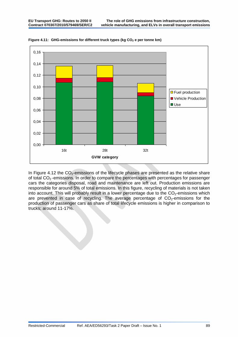
EU Transport GHG: Routes to 2050 II The role of GHG emissions from infrastructure construction, Contract 070307/2010/579469/SER/C2 vehicle manufacturing, and ELVs in overall transport emissions
Restricted-Commercial Ref. AEA/ED56293/Task 2 Paper Draft – Issue No. 1 89
Figure 4.11: GHG-emissions for different truck types (kg CO2 e per tonne km)
0,00
0,02
0,04
0,06
0,08
0,10
0,12
0,14
0,16
16t 28t 32t
GVW category
Fuel production
Vehicle Production
Use
In Figure 4.12 the CO2-emissions of the lifecycle phases are presented as the relative share of total CO2 -emissions. In order to compare the percentages with percentages for passenger cars the categories disposal, road and maintenance are left out. Production emissions are responsible for around 5% of total emissions. In this figure, recycling of materials is not taken into account. This will probably result in a lower percentage due to the CO2-emissions which are prevented in case of recycling. The average percentage of CO2-emissions for the production of passenger cars as share of total lifecycle emissions is higher in comparison to trucks; around 11-17%.

The role of GHG emissions from infrastructure construction, EU Transport GHG: Routes to 2050 II vehicle manufacturing, and ELVs in overall transport emissions Contract 070307/2010/579469/SER/C2
Restricted-Commercial Ref. AEA/ED56293/Task 2 Paper Draft – Issue No. 1 90
Figure 4.12: Contribution of different stages in the life cycle to total GHG emissions (%CO2e)
0%
10%
20%
30%
40%
50%
60%
70%
80%
90%
100%
16t 28t 32t
GVW category
Fuel production
Vehicle Production
Use
Facanha and Horvath (2007) have compared the life-cycle emission factors related to road, rail and air transportation of freight in the United States. The study includes all life-cycle phases and is focused on long-distance transportation. In Figure 4.13 the share of emissions is presented for all life-cycle phases. CO2 emissions related to the vehicle (production) have a share of 10% of overall life cycle emissions. Like for passenger cars CO2 is mostly emitted in the vehicle use phase. Increasing vehicle fuel efficiency and reducing emission factors from fuel combustion emissions will therefore be most effective in reducing the total emissions, rather than reducing CO2 emissions in the manufacturing phase of trucks. The study does not provide details about the vehicle production stage and total mileage assumed.

EU Transport GHG: Routes to 2050 II The role of GHG emissions from infrastructure construction, Contract 070307/2010/579469/SER/C2 vehicle manufacturing, and ELVs in overall transport emissions
Restricted-Commercial Ref. AEA/ED56293/Task 2 Paper Draft – Issue No. 1 91
Figure 4.13: Share of life-cycle phases in transportation air emissions (Facanha and Horvath, 2007)
Gaines et al. (1998) shows that lower tailpipe emissions do not necessarily implicate lower total lifecycle emissions. The study considered the largest category of US trucks; over-the-road tractor semitrailer combinations (18-wheelers) weighing over 26,000 lb. Most trucks in this category weigh 60,000-80,000 lb. The study found 38 g CO2e/vkm for vehicle production, assuming a lifetime mileage of 1,2 million kilometres. This roughly corresponds with the values for the 40t truck from the Ecoinvent database, presented above, if corrected for the lifetime mileage and the use of recycled materials by Gaines et al (1998). The study dhows that weight reduction of 15-20% can be achieved if aluminium and magnesium are used. This kind of weight reduction would lead to a reduction in the fuel consumption. The study calculated the impact of a mass reduction of 1 tonne on the total lifecycle emissions. It concludes that the lifetime impacts are limited (1-3%), but depending the type of goods shipped. Replacing steel by aluminium in order to decrease the weight of a truck leads to slightly higher energy use. Concerning CO2-emissions the manufacturing of trucks results in relatively lower emissions compared to passenger cars. Approximately 5% of the total emissions (vehicle production, fuel production and vehicle use) can be accounted to the manufacturing of trucks. The percentage can even decrease in case the use of recycled materials increases. The relative share of production emissions can rise in the future when fuel efficiency will increase and cleaner fuels will be used. On the other hand vehicle production will probably also become more sustainable and recycling options will be developed further.
4.1.2 References
AEA (2007) Hybrid Electric and Battery Electric Vehicles, Technology, Costs and benefits, November 2007
The role of GHG emissions from infrastructure construction, EU Transport GHG: Routes to 2050 II vehicle manufacturing, and ELVs in overall transport emissions Contract 070307/2010/579469/SER/C2
Restricted-Commercial Ref. AEA/ED56293/Task 2 Paper Draft – Issue No. 1 92
CE Delft (2010) Green Power for Electric Cars: Development of policy recommendations to harvest the potential of electric vehicles, Delft, January 2010 Facanha, C and Horvath, A (2007)„Evaluation of Life-Cycle Air Emission Factors of Freight Transportation’, ICF International, Department of Civil and Environmental Engineering, University of California L. Gaines, F. Stodolsky, and R. Cuenca (1998) Argonne National Laboratory Transportation Technology R&D Center, Office of Heavy Vehicle Technologies U.S. Department of Energy, „Life-Cycle Analysis for Heavy Vehicles’ JEC (2008) Well-to-Wheels analysis of future automotive fuels and powertrains in the European context, EUCAR / JRC / CONCAWE Helms, H., Pehnt, M., Lambrecht, U. and Liebich, A, (2010) Electric vehicle and plug-in hybrid energy efficiency and life cycle emissions, Ifeu – Institut für Energie- und Umweltforschung, Wilckensstr. 3, D-69120 Heidelberg. 18th International Symposium Transport and Air Pollution Session 3: Electro and Hybrid Vehicles, page 113 from 274. 2010. Notter, D.A. et al., (2010) Contribution of Li-Ion Batteries to the Environmental Impact of Electric Vehicles, EMPA, Switzerland, in Environ. Sci. Technol. 2010, 44, 6550–6556 Samaras, C and Meisterling, K (2009) Life Cycle Assessment of Greenhouse Gas Emissions from Plug-in Hybrid Vehicles: Implications for Policy, Environ. Sci. Technol., 2008, 42 (9), 3170-3176 • DOI: 10.1021/es702178s • Publication Date (Web): 05 April 2008 Schweimer, G.W (2000) Life Cycle Inventory for the Golf A4, Research, Environment and Transport, Volkswagen AG, Wolfsburg, Marcel Levin, Center of Environmental Systems Research, University of Kassel J. Smidt and R. Leithner, (1995) „Automobilrecycling’ Berlin : Springer-Verlag, 1995. Spielmann, M., Bauer, C., Dones, R., Tunchschmid, M. (2007) Transport Services ecoinvent report no 14. Swiss Centre for Life Cycle Inventories, Dübendorf, 2007 TNO (2006) Review and analysis of the reduction potential and costs of technological and other measures to reduce CO2-emissions from passenger cars, Final Report, Contract nr. SI2.408212 Delft, October 31, 2006 TNO et al, (2010) (draft report) Support for the revision of Regulation (EC) No 443/2009 on CO2 emissions from cars Service request #1 for Framework Contract on Vehicle Emissions Framework Contract No ENV.C.3./FRA/2009/0043 Draft Interim report Date: March 7, 2011 Marco F. Torchio, a, and Massimo G. Santarellia, (2010) Energy, environmental and economic comparison of different powertrain/fuel options using well-to-wheels assessment, energy and external costs – European market analysis. 2010. VW (2009a) The Golf Environmental Commendation, detailed version VW (2009b) The Passat Environmental Commendation, detailed version Zackrisson, M., Avellán, L., and Orlenius, J (2010) Life cycle assessment of lithium-ion batteries for plug-in hybrid electric vehicles – Critical issues.

EU Transport GHG: Routes to 2050 II The role of GHG emissions from infrastructure construction, Contract 070307/2010/579469/SER/C2 vehicle manufacturing, and ELVs in overall transport emissions
Restricted-Commercial Ref. AEA/ED56293/Task 2 Paper Draft – Issue No. 1 93
4.2 Rail
4.2.1 Summary of information from the literature
A number of studies are available in the literature that assesses the lifecycle emissions from rail rolling stock production, operation and disposal. The breakdown of embedded GHG emissions due to the materials used to construct rail vehicles is dominated by the use of steel and aluminium in both heavy and light rail vehicles – see Figure 4.14.
Figure 4.14: Breakdown of material use for a light and heavy electric rail vehicle
57.3%
26.7%
2.5%7.3%
1.7% 1.3%
3.1%
Heavy Rail VehicleSteel
Aluminium
Copper
Plastic
Glass
Lubricating oil
Wood
54.3%
14.5%1.0%
18.6%
3.4%5.4% 2.8%
Light Rail VehicleIron alloys
Nonferrous metals
Inorganic materials
Plastics
Other materials
Organic substances
Electronics
Source: Heavy vehicle estimates based on electric multiple unit material breakdown from AEA (2007).
Light rail vehicle estimates based on data from Siemens (2010)
However, it can be difficult at times to compare different studies due to different boundaries, methodologies and coverage. For example, some studies, like UIC (2009) incorporate significant estimates for energy and emissions resulting from major revisions to heavy rail rolling stock. These can account for a significant component of the total for the lifetime of the vehicle‟s operation, as illustrated in Figure 4.15. However, these emissions do not appear to be included in some other studies.
Figure 4.15: Energy consumption and GHG emissions from the lifecycle of a high speed train
61.1%
2.9%
35.8%
0.2%Energy
Production of train
Maintenance & Cleaning of a ICE
Revision of ICE
Disposal
55.1%
3.4%
40.8%
0.8%GHG
Production of train
Maintenance & Cleaning of a ICE
Revision of ICE
Disposal
Source: UIC (2009)
Unlike most of the studies identified, the assessment from ADEME (2010) also included an estimate of the greenhouse gas emissions resulting from the energy consumption from the manufacture of the rolling stock, in addition to the usual assessment of emissions due to

The role of GHG emissions from infrastructure construction, EU Transport GHG: Routes to 2050 II vehicle manufacturing, and ELVs in overall transport emissions Contract 070307/2010/579469/SER/C2
Restricted-Commercial Ref. AEA/ED56293/Task 2 Paper Draft – Issue No. 1 94
material use. As illustrated in Figure 4.14, this is a significant component accounting for 41% of the assessed total GHG emissions from manufacture.
Figure 4.16: Breakdown of material use for a light and heavy electric rail vehicle
Mater-ials59%
Energy41%
TGV-Duplex Production, tCO2
Source: ADEME (2010)
Different methodologies of accounting for materials, energy and emissions at different lifecycle stages can also lead to quite different results. For example, in Figure 4.17 is presented estimates of the emissions from production and disposal of an electric railcar based on two alternative methodologies of accounting for recycled material – (i) the production emissions estimated on the basis of average recycled content of materials, or (ii) the total net emissions calculated on the basis of virgin materials, plus 80% recycling at the end of life. As can be seen, these different approaches give quite different results.
Figure 4.17: Breakdown of material use, production and disposal GHG emissions by material for an electric rail vehicle
27.167.3 83.9
-28.10.1
-28.1
55.812.6
108.7
138.6
-90.7
0.0
-90.7
47.9
-150
-100
-50
0
50
100
150
200
250
300
Tonnes Material
CO2e: Production (recycled content)
CO2e: Production
(virgin material)
CO2e: Recycling
CO2e: Other Disposal
CO2e: End of Life Total
Net CO2e: Production + End of Life
To
nn
es b
y M
ate
rial T
yp
e
Steel Aluminium Copper Glass Lubricating oil Wood Plastic
Notes: Estimates based on electric multiple unit material breakdown from AEA (2007). Assumes 80% recycling for breakdown of net figure.

EU Transport GHG: Routes to 2050 II The role of GHG emissions from infrastructure construction, Contract 070307/2010/579469/SER/C2 vehicle manufacturing, and ELVs in overall transport emissions
Restricted-Commercial Ref. AEA/ED56293/Task 2 Paper Draft – Issue No. 1 95
In terms of the relative significance of GHG emissions from the different lifecycle phases of the train, reasonable comparability between different studies can be achieved through normalising to the same electricity emission factor. The following Figure 4.18 provides a comparison of the relative significance of emissions from the train construction, maintenance and operational phases. This clearly illustrates the over-riding significance of operational energy consumption, which accounts for around 95% of all emissions resulting from the train lifecycle assuming an average EU electricity mix over a 30-year operational lifetime. For highly decarbonised electricity mixes this proportion will be lower. The train construction and maintenance phases are dominated by the emissions resulting from the production of steel and aluminium. Therefore it seems unlikely this balance would change significantly in the future given these materials and electricity generation are all likely to significantly decarbonise by 2050. However, some studies suggest that an increasing use of composite materials (like carbon fibre reinforced plastic) to reduce vehicle weight may alter the balance somewhat, as these currently require large amounts of energy to produce, but have low end of life recyclability (Lee, 2010). The degree to which this may alter the balance of emissions between construction/disposal and operation is at the moment uncertain. TBC after focus group meeting…
Figure 4.18: Breakdown of GHG emissions across the lifecycle of different train models
96.9% 95.1% 94.9% 92.9% 94.0%
0%
10%
20%
30%
40%
50%
60%
70%
80%
90%
100%
Shinkansen ICE TGV-Duplex Hitachi Super Express
AGV
KATO (2005) UIC (2009) ADEME (2010) AEA (2011)
% o
f T
rain
Lif
ecycle
GH
G e
mis
sio
ns
Train construction Train maintenance and repair Train operation
Notes: Estimates based on information collected from different literature sources, with train operational emissions normalised to projected 30-year average EU electricity mix between 2010 and 2040.

The role of GHG emissions from infrastructure construction, EU Transport GHG: Routes to 2050 II vehicle manufacturing, and ELVs in overall transport emissions Contract 070307/2010/579469/SER/C2
Restricted-Commercial Ref. AEA/ED56293/Task 2 Paper Draft – Issue No. 1 96
Table 4.10: Comparison of typical current and future conventional (intercity) and high-speed rail rolling stock
Type of train Conventional Rail (Intercity) High Speed Rail
Train Model Class 91
IC225
Class 390 Pendolino
Hitachi Super
Express
Class 373
Eurostar
TGV Reseau
TGV Duplex
AVE S103 Velaro
Shinkan-sen 700 Series
AGV
Year 1989 2003 Future 1993 1992-6 1995-7 2004 1998 Future
Max Speed 200 225 200 300 300 300 350 300 350
Service Speed 200 200 200 300 300 300 300 300 300
Seating Capacity 536 439 649 750 377 545 404 1323 650
Length (m) 247 215 260 394 200 200 200 400 250
Vehicles per unit 11 9 10 20 10 10 8 16 14
Tare mass (tonnes) 498 460 412 723 386 384 425 634 510
Mass per vehicle (tonnes)
45.3 51.1 41.2 36.2 38.6 38.4 53.1 39.6 36.4
Mass per train metre (tonnes)
2.02 2.14 1.58 1.84 1.93 1.92 2.13 1.59 2.04
Mass per seat (tonnes) 0.93 1.05 0.63 0.96 1.02 0.70 1.05 0.48 0.78
Energy consumption (kWh/seat-km)
0.035 0.033 0.028 0.041 0.039 0.037 0.039 0.029 0.033
GHG emissions (kgCO2e/seat-km)*
0.0074 0.0070 0.0059 0.0087 0.0083 0.0079 0.0082 0.0062 0.0070
Improvement over historic stock
N/A N/A 20% N/A N/A N/A N/A N/A 15%
Source: Estimates based information from AEA (2007).
Notes: * Calculated based on projected 30-year average EU electricity mix between 2010 and 2040.
4.2.2 Identification of gaps – focus group
Gaps in the literature which the focus group may be able to add to:
Possible differences between electric and diesel rolling stock;
The extent to which composite materials are likely to replace existing materials (steel,
aluminium in future rail rolling stock design.
4.2.3 References
ADEME (2010). 1st Bilan Carbone - global railway carbon footprint, 2010. Available at: http://bilan-carbone-lgvrr.fr/en/information-documents
AEA (2011). Updated analysis by AEA based on work carried out for Network Rail (AEA 2009).
AEA (2009): Comparing environmental impact of conventional and high speed rail, a report by AEA for Network Rail, 2009. Available at: http://www.networkrail.co.uk/aspx/5892.aspx
KATO (2005). A life cycle assessment for evaluating environmental impacts of inter-regional high-speed mass transit projects, by Hirokazu KATO, Naoki SHIBAHARA, Motohiro OSADA, and Yoshitsugu HAYASHI, Journal of the Eastern Asia Society for Transportation Studies, Vol. 6, pp. 3211 - 3224, 2005, available at: http://www.easts.info/on-line/journal_06/3211.pdf
Lee (2010). Assessing environmentally friendly recycling methods for composite bodies of railway rolling stock using life-cycle analysis, Cheul-Kyu, Lee et al, Transportation Research

EU Transport GHG: Routes to 2050 II The role of GHG emissions from infrastructure construction, Contract 070307/2010/579469/SER/C2 vehicle manufacturing, and ELVs in overall transport emissions
Restricted-Commercial Ref. AEA/ED56293/Task 2 Paper Draft – Issue No. 1 97
Part D: Transport and Environment, Volume 15, Issue 4, June 2010, Pages 197-203. Available from: http://trid.trb.org/view.aspx?id=917779
Siemens (2011). Metro Oslo - Environmental Product Declaration according to ISO 14021, downloaded April 2011: http://www.industry.siemens.com/topics/global/de/environmental-care/energieeffizienz/case-metro-oslo/Documents/oslo_umweltdeklaration_en.pdf
UIC (2009). Carbon Footprint of High-Speed railway infrastructure (Pre-Study) - Methodology and application of High Speed railway operation of European Railways. A report for the International Union of Railways (UIC), 2010. Available from UIC‟s website at: http://www.uic.org/IMG/pdf/carbon_footprint_of_high_speed_rail_infrastructure_pre-study.pdf
4.3 Aviation
4.3.1 Summary of information from the literature
The primary GHG emissions and energy factors in the manufacturing of aircraft are related to the electricity used at the manufacturing facilities and the diesel fuel consumed in truck transportation moving parts for assembly (EIOLCA, 2007). The GHG effects of vehicle manufacturing typically account for between 5-11% of aircraft life-cycle GHG emissions. For smaller vehicles, such as the Embraer 145, the emissions produced during manufacturing are smaller than for larger aircrafts, such as the Boeing 747. This is due to the larger amount of materials needed to manufacture a 397,900 lbs Boeing 747 compared to the 5,335 lbs Embraer 145. However, as shown in Figure 4.19, GHG emissions from manufacturing may be smaller for smaller aircraft but spread out over fewer passenger-mile-travelled (PMT) over the life-cycle of an aircraft.
Figure 4.19: Life Cycle Assessment of Passenger Transportation (GHG emissions in g/PMT) (Chester and Horvarth, 2007)
The manufacturing process of an aircraft vehicle consists of six major subassemblies: the fuselage or body; the empennage or tail assembly; the wings, the landing gear assemblies, the powerplant (jet engine) and the flight control systems and instruments. Although using a similar assembly line process to the automotive sector for manufacturing vehicles, production volume is much lower in aircraft manufacturing.

The role of GHG emissions from infrastructure construction, EU Transport GHG: Routes to 2050 II vehicle manufacturing, and ELVs in overall transport emissions Contract 070307/2010/579469/SER/C2
Restricted-Commercial Ref. AEA/ED56293/Task 2 Paper Draft – Issue No. 1 98
The manufacturing of aircrafts is a systematic series of „positions‟ and „setbacks‟, where, for example, a wing assembly may only encompass one position, but within this position there may be three setbacks. Environmental protection laws have developed stringent codes limiting water flows and emissions from aircraft manufacturing facilities. The use of solvents and cleaning processes in particular can benefit from environmental processes, such as steam vapour degreasing systems. In compliance with federal laws, aircraft companies have been using fewer solvents and looking for better ways to clean parts, such as steam vapour degreasing systems29.
Figure 4.20: Airbus Main Manufacturing Impacts30
The EIOLCA (Economic Input-Output Life Cycle Assessment) method estimates the materials and energy resources required for, and the environmental emissions resulting from, activities including aircraft manufacturing (EioLCA, 2007). The manufacturing of aircraft results in large CAP emissions (where not so significantly for rail modes). About 70% of SO2 and 40% of manufacturing NOX result in electricity generation during aircraft manufacturing. Around 50% of CO emissions and 20% of VOC emissions in manufacturing result from truck transportation in transporting parts and materials for final assembly (EioLCA, 2007). Vehicle manufacturing accounts for between
8% to 36% of SO2;
7% to 48% of CO;
29
http://www.madehow.com/Volume-2/Business-Jet.html 30
http://www.obsa.org/Lists/Documentacion/Attachments/144/Part_II_Enviromental_EN.pdf

EU Transport GHG: Routes to 2050 II The role of GHG emissions from infrastructure construction, Contract 070307/2010/579469/SER/C2 vehicle manufacturing, and ELVs in overall transport emissions
Restricted-Commercial Ref. AEA/ED56293/Task 2 Paper Draft – Issue No. 1 99
1% to 7% of NOX;
9% to 42% of VOC;
58% to 90% of Pb; and
8% to 41% of PM10 total life-cycle emissions (ECOLCA, 2007).
As shown in Figure 4.19, the smaller percentages relate to the Boeing 737, the larger percentage the Boeing 747, and the Embraer 145 lies between the two. The lead (Pb) emissions, which make up the majority of total emissions, result from the production of nonferrous metals for the aircraft during the manufacturing process. As part of the manufacturing process, Airbus introduced the "base coat, clear coat" painting method, which requires only one layer of thick paint and a layer of varnish or clear coat for protection (Davies, 2011). Standard methods can require up to six coats of paint, thus the Airbus method shows a significant reduction. In connection with this reduction in paint volume, manufacturing infrastructure reduces the emissions produced as part of the vehicle painting process. An optimised ventilation system reduces energy consumption by 50,000 kilowatt hours during the average 16-day processing time for an A380 aircraft – a 32-tonne reduction of CO2 per plane. Airbus is one of the world's leading commercial and military aircraft manufacturers. The company's own manufacturing, production and sub-assembly of parts for Airbus aircraft are distributed around 15 sites in Europe. Final assembly production of aircraft takes place in France, Germany, Spain and since 2009, China. Airbus Transport International, operates the five A300-600ST Super Transporters, (nicknamed Belugas) used to carry aircraft sections between the different European manufacturing sites shown in Figure 4.21. Based in France, it is licensed for world-wide cargo charter operations and, since its creation in 1996, has successfully transported parts from Airbus‟ manufacturing facilities in Europe to the final assembly lines in Toulouse and Hamburg. For the A380, aircraft components are shipped via a multimodal transport network that combines marine, river and road transport, when they are far too large for the Belugas. In the future, larger aircrafts may be temporarily limited in their transportation as a result of current infrastructure limitations which would need to be modified.

The role of GHG emissions from infrastructure construction, EU Transport GHG: Routes to 2050 II vehicle manufacturing, and ELVs in overall transport emissions Contract 070307/2010/579469/SER/C2
Restricted-Commercial Ref. AEA/ED56293/Task 2 Paper Draft – Issue No. 1 100
Figure 4.21: Airbus Transportation of the A380 sections
The impact on climate change of CFRP (carbon-fibre-reinforced-polymer) stands as the most environmental harmful process of the manufacturing of aircraft (56.6% in relation to the global processes contribution), despite being far less used that aluminium or steel that have a combined contribution of 21.6% to the total process contribution. CFRP only represents 9% of the aircraft weight, as shown in Figure 4.22, but is by far the largest composite in use according to a life-cycle assessment study of an A330-200 (Lopes, 2010).
Figure 4.22: Generic material breakdown of aircraft A330-200, including main and nose landing gears and engines (Lopes, 2010).
An NSF International & Trucost report based on information from 37 aerospace manufacturing companies, each of which had operations in FY2007, looked at the impacts of aircraft manufacturing. The report includes the following manufacturing industries: aircraft, aircraft engine and engine parts, other aircraft parts and auxiliary equipment.

EU Transport GHG: Routes to 2050 II The role of GHG emissions from infrastructure construction, Contract 070307/2010/579469/SER/C2 vehicle manufacturing, and ELVs in overall transport emissions
Restricted-Commercial Ref. AEA/ED56293/Task 2 Paper Draft – Issue No. 1 101
The average aerospace company in the Trucost database (4,500 companies) had revenues of about $17 billion and GHG emissions of 4 million tCO2-e in 2007. Trucost uses the GHG protocol corporate accounting standard which recognises GHG emissions into Scope 1, 2 and 3 whereby:
Scope 1: Direct GHG caused by a company‟s fuel combustion or emitted through industrial processes owned or controlled by a company.
Scope 2: Indirect GHG emissions from purchased electricity.
Scope 3: Indirect emissions from suppliers (other than electricity suppliers) that provide goods or services purchased by a company.
Figure 4.23 shows that across these three scopes, the majority (93%) of GHG emissions from aerospace manufacturers originates from within the supply chain. Whilst 7% is from electricity suppliers, 86% is from other suppliers within the supply chain.
Figure 4.23: Scope 1-3 GHG Emissions Aerospace Manufacturing Sector (tCO2-e) (NSF, 2008)
According to the Trucost database, around 60% of aerospace manufacturers do not report their emissions. Of those which report their emissions, companies that are more carbon efficient and have lower carbon intensity that their peers will be better positioned to succeed in the face of GHG regulatory costs. As shown in Figure 4.24, the range in carbon intensities in the aerospace manufacturing industry is moderate, running from 115 tCO2-e/US$m revenue to over three times that amount (384 tCO2-e/US$m).

The role of GHG emissions from infrastructure construction, EU Transport GHG: Routes to 2050 II vehicle manufacturing, and ELVs in overall transport emissions Contract 070307/2010/579469/SER/C2
Restricted-Commercial Ref. AEA/ED56293/Task 2 Paper Draft – Issue No. 1 102
Figure 4.24: Range in aerospace manufacturer carbon intensity (tCO2e/US$m revenue) (NSF, 2008)
The widespread network of manufacturing plants required to manufacture aircrafts results in transport emissions. Emissions from the manufacture of composites are significant due to this logistical factor as well as a result of the high temperatures required to produce carbon fibres. The advanced composite process of autoclave modelling produces denser, void free modelling but requires higher hear and pressure during the curing process. Manufacturing composites in autoclaves is estimated to produce 2% of NOx emissions by weight (Omega, 2011). Shelf life and storage of composite pre-manufactured uncured tape (prepreg) and constituent raw materials required from this process also produced emissions although the civil aircraft manufacturing industry uses a „just in time‟ approach that cannot be applied in military applications. Integrated approaches between different industrial sectors involved in air transport manufacturing offers improved efficiencies. This has been demonstrated through the Airbus ACADEMY project that which successfully piloted new methods for adapting the EU‟s Eco-Management and Audit Scheme (EMAS) to its aeronautical corporate partners31. Although Europe‟s aeronautical sector contains around 100,000 businesses, less than five percent of EU companies in the sector are certified with ISO 14001 standards and intricate life cycles involved in manufacturing aircraft products have previously presented obstacles that inhibited wider cooperation32.
Opportunities to reduce emissions from manufacturing process in the future
Carbon Fibre - When looking at future materials in the manufacturing of aircrafts, carbon fibre is likely to play a key role in reducing GHG emissions and fuel consumption. Grob Aerospace built a SPn business aircraft entirely from carbon fibre, using low temperature and pressure curing processes. In terms of both manufacturing and operation, the all composite SPn light business het is one of the greenest aircrafts ever built in its category. Compared to aluminium fuselage and wing manufacturing, the carbon fibre alternative is less energy intensive as a result of lower temperatures and pressures during the curing processes. Grob Aerospace's "wet-in-wet" technology developed to cure aircraft composite structures is inherently energy efficient because it does not require high-temperature autoclaves for curing. Instead, structures are cured at relatively low temperatures of 60-80oC. This gives up to a 25% reduction in primary energy consumption for the production of the SPn airframe compared to an all-aluminium airframe structure33.
31
(LIFE04 ENV/FR/000353) 32
http://ec.europa.eu/environment/life/themes/management/features2010/airtransport.htm 33
http://www.airframer.com/news_story.html?release=2124

EU Transport GHG: Routes to 2050 II The role of GHG emissions from infrastructure construction, Contract 070307/2010/579469/SER/C2 vehicle manufacturing, and ELVs in overall transport emissions
Restricted-Commercial Ref. AEA/ED56293/Task 2 Paper Draft – Issue No. 1 103
Composite construction compared with aluminium places lower demands on the use of raw materials and energy in its processes. 33kg of basic raw materials are required to produce 1kg of the final product of an aluminium aircraft, whereas only 5kg of raw materials are required to produce 1kg of the final product of a SPn33. In addition, when comparing the carbon fibre SPn manufacturing process to that of all-aluminium airframes, SPn achieves up to an 82% savings in residues from ore extraction and between 67% and 90% lower use of non-regenerative resources. Furthermore, the limited use of chemical solvents during the carbon fibre production process leads to a 16-28% lowering in emissions from NMVOC33. For the production of metal aircraft, an anodic oxidation protective coating is required against corrosion, which is highly energy intensive, contains chromic acids and causes highly toxic waste waters. In the production of aircraft made of carbon fibre none of these toxic substances are used. Mechanical Milling of Fuselage Panels (LIFE 05 ENV/F/000062) - In conjunction with Dufieux Industrie, Airbus have developed a new milling machine which produces nose fuselage panels 50% faster and cheaper than traditional methods and thus lowers environmental impacts. Reducing the thickness of aluminium aircraft panels is traditionally a labour intensive milling process which requires using a chemical bath, producing hazardous by-products34. Introduced in 2006 under the European Commission‟s LIFE Programme, the alternative non-chemical process produces only aluminium shavings as a by-product which are collected, recycled and sold back to the supplier. When considering the future impact of emissions from manufacturing as a result of this technology, the following yearly eco-efficiency benefits should be considered35:
Water savings of 225,000 m3 per year equivalent to the consumption of a city of 4,000 inhabitants;
Waste reduction of >16,000 tonnes (hazardous and domestic waste);
50% gain on operating costs;
20% gain on cost of each manufactured unit;
50% gain on production cycle time; and
57% economy on electricity consumption. Bombardier Aerospace Belfast has contributed research to the Next Generation Composite Wing (NGCW) Programme which brings 17 organisations together on the development of future composite wing technologies36. The Irish company are responsible for the design, development, certification and manufacture of the CSeries carbon composite outer wing, including the control surfaces and the integration of the wing systems. The Resin Transfer Infusion (RTI) process used is a hybrid of Resin Transfer Moulding (RTM) and autoclave processing. It uses dry fabrics to create the structure and then injects resin into the structure once it is placed in the autoclave, resulting in material savings and reduced cycle times36. The carbon fibre composites used as part of this process reduce the airframe weight to make a direct contribution to both fuel burn and operating efficiency of aircrafts. A quantified emissions saving when compared with all-aluminium alternatives is not known. The European Commission‟s Clean Sky Joint Technology Initiative (JTI)37 of February 2008 was designed to stimulate research, development and deployment of technology to reduce GHG emissions from aviation. With implementation years between 2008 and 2013, the initiative will have an impact on manufactures of aircraft in the future38. 34
Mechanical Milling of Fuselage Panels (LIFE 05 ENV/F/000062) http://ec.europa.eu/environment/life/themes/water/lists/scarcity.htm 35
http://www.obsa.org/Lists/Documentacion/Attachments/144/Part_II_Enviromental_EN.pdf 36
http://www.aero-mag.com/features/19/20099/105/ 37
Clean Sky Join Technology Initiative http://www.cleansky.eu/ 38
http://www.flightglobal.com/articles/2010/10/05/348002/europes-clean-sky-programme-confident-of-achieving-engine-
demonstrator.html

The role of GHG emissions from infrastructure construction, EU Transport GHG: Routes to 2050 II vehicle manufacturing, and ELVs in overall transport emissions Contract 070307/2010/579469/SER/C2
Restricted-Commercial Ref. AEA/ED56293/Task 2 Paper Draft – Issue No. 1 104
Objectives include developing technologies that will allow reductions in aviation CO2 emissions by 50% through fuel efficiencies and reductions in NOx emissions by 80% by 2020. The public-private partnership also seeks to establish a "green" product life cycle, from the design to the disposal/recycling of materials and components38. As part of the initiative, six Integrated Technology Demonstrators (ITDs) have been targeted: Smart fixed-wing aircraft - Focus is on an innovative "smart wing" design and the integration of novel engine concepts, including the resulting modifications of the aircraft. The goal is to reduce the medium- and long-range aircraft fuel burn and emissions by around 10% to 20%. Green regional aircraft - The objective is to validate and demonstrate the technologies best fitting the pollution and noise reduction goals set for the regional aircraft that will enter the market in the 2020s. This includes using new structures and materials to reduce weight, configurations for low aerodynamic noise, and the integration of technologies developed in other ITDs. Green rotorcraft - Rotorcrafts are flying machines that use rotorblades, including helicopters and gyroplanes. The demonstration of diesel engine integration, airframe drag minimisation features and advanced electrical systems will enable the reduction of fuel consumption and elimination of noxious hydraulic fluids in these vehicles. Sustainable and green engines - This ITD addresses engine design, noise reduction, NOx emissions reductions, and reduced fuel use. System for green operations - This ITD creates value for improved aircraft operation through the management of aircraft energy and the management of mission and trajectory. Eco-design - This ITD implements a strategy for design, development, manufacturing, use and recycling, covering airframes and systems38. Ubiquitously across aircraft engine manufacturers, the design goal is to boost propulsive and thermal efficiency to reduce fuel burn and carbon dioxide emissions. However, this involves designing a larger engine fan and a smaller core, which presents the unwanted issue of increased weight. The ITD target this problem to ensure that future aircraft manufacturing can meet demand whilst minimising the impact of aviation on global GHG emissions. When considering aircraft engines, 99.9% of the GHG emissions associated with a typical aircraft engine occur during the „in-service‟ life cycle phase. As shown in the normalised figures in Figure 4.25, when considering the emissions from the engine use as 1, less than 0.001 of the GHG emissions are a result of the manufacturing process.

EU Transport GHG: Routes to 2050 II The role of GHG emissions from infrastructure construction, Contract 070307/2010/579469/SER/C2 vehicle manufacturing, and ELVs in overall transport emissions
Restricted-Commercial Ref. AEA/ED56293/Task 2 Paper Draft – Issue No. 1 105
Figure 4.25: Normalised GHG Emissions from life-cycle stage of typical aircraft engine
Source: Rolls-Royce (Personal contact with Nigel Marsh, Rolls-Royce)
However, when looking at engine manufacturing as part of the wider aircraft manufacturing process, the environmental impact is significant. A life-cycle study of an A330-200 found that despite representing only 17% of the total aircraft weight, the engine structure emerged as having the largest contribution for many environmental impact categories over the manufacturing of other components. These included metal depletion, urban land occupation and particulate matter formation39.
4.3.2 Development of emission factors for the analysis
A study of aircraft manufacturing materials, the Probe database, assumes aircrafts consist of two main types of materials: aluminium and hard plastic. The weight distribution in tonnes is shown below:
Table 4.11: Weight distribution of domestic and international aircrafts. Assumptions from Probe database (tonnes) (Simonsen, 2011)
Weight in tons. Domestic International
Aluminium 55 216
Hard Plastic 6 24
Total 61 240
39
https://dspace.ist.utl.pt/bitstream/2295/792342/1/Tese_JoaoVascoLopes.pdf

The role of GHG emissions from infrastructure construction, EU Transport GHG: Routes to 2050 II vehicle manufacturing, and ELVs in overall transport emissions Contract 070307/2010/579469/SER/C2
Restricted-Commercial Ref. AEA/ED56293/Task 2 Paper Draft – Issue No. 1 106
Table 4.12: Emissions to air during production and transportation of materials to Airbus 320, Airbus A340-600, Boeing 737-300 and Embraer 145 (Simonsen, 2011)
Airbus A320 Aluminium (tons) Hard plastic (tons) Total
Airbus A320
CH4 2.0 0.03 2.0
CO2 480.1 20.08 500.1
N2O 0.0 0.00 0.0
CO2e 643.9 21.0 664.8
Airbus A340-600
CH4 8.4 0.11 8.5
CO2 2007.2 84.61 2091.8
N2O 0.1 0.00 0.1
CO2e 2692.2 88.3 2780.5
Boeing 737-300
CH4 1.6 0.02 1.6
CO2 373.4 15.61 389.0
N2O 0.0 0.00 0.0
CO2e 500.8 16.30 517.1
Embraer 145
CH4 0.6 0.01 0.6
CO2 132.4 5.54 137.9
N2O 0.0 0.00 0.0
CO2e 177.6 5.78 183.4
Table 4.13: Energy consumption in the production and transportation of materials to Airbus 320, Airbus A340-600, Boeing 737-300 and Embraer 145 (Simonsen, 2011)
Energy Consumption Aluminium GJ Hard-plastic GJ Sum
Airbus A320
Nuclear power 911 42 953
Biomass 64 2 66
Lignite (Brown coal) 522 37 559
Natural gas 1,745 85 1,830
Oil 1,059 61 1,120
Geothermal 0 0 0
Waste 126 12 138
Secondary raw material -7 -13 -21
Solar Energy 1 0 1
Hard coal 1,577 5 1,582
Hydropower 674 2 676
Wind Power 28 1 28
SUM 6,701 234 6,934
Airbus A340-600
Nuclear power 3,807 179 3,986
Biomass 268 7 275
Lignite (Brown coal) 2,182 156 2,338

EU Transport GHG: Routes to 2050 II The role of GHG emissions from infrastructure construction, Contract 070307/2010/579469/SER/C2 vehicle manufacturing, and ELVs in overall transport emissions
Restricted-Commercial Ref. AEA/ED56293/Task 2 Paper Draft – Issue No. 1 107
Energy Consumption Aluminium GJ Hard-plastic GJ Sum
Natural gas 7,296 359 7,655
Oil 4,429 257 4,685
Geothermal 0 0 0
Waste 529 50 578
Secondary raw material -30 -57 -87
Solar Energy 5 0 5
Hard coal 6,595 21 6,616
Hydropower 2,820 9 2,828
Wind Power 115 4 119
SUM 28,016 984 29,000
Boeing 737-300
Nuclear power 708 33 741
Biomass 50 1 51
Lignite (Brown coal) 406 29 435
Natural gas 1,357 66 1,424
Oil 824 47 871
Geothermal 0 0 0
Waste 98 9 108
Secondary raw material -6 -10 -16
Solar Energy 1 0 1
Hard coal 1,227 4 1,231
Hydropower 525 2 526
Wind Power 21 1 22
SUM 5,212 182 5,393
Embraer 145
Nuclear power 251 12 263
Biomass 18 0 18
Lignite (Brown coal) 144 10 154
Natural gas 481 24 505
Oil 292 17 309
Geothermal 0 0 0
Waste 35 3 38
Secondary raw material -2 -4 -6
Solar Energy 0 0 0
Hard coal 435 1 436
Hydropower 186 1 187
Wind Power 8 0 8
SUM 1,848 64 1,913

The role of GHG emissions from infrastructure construction, EU Transport GHG: Routes to 2050 II vehicle manufacturing, and ELVs in overall transport emissions Contract 070307/2010/579469/SER/C2
Restricted-Commercial Ref. AEA/ED56293/Task 2 Paper Draft – Issue No. 1 108
Table 4.14: Energy & GHG emissions from aircraft and aircraft engine manufacturing (Simonsen, 2011)
Manufacturing Energy Unit GHG (CO2e) Unit
Small Aircraft 63 TJ/plane 5.1 kg/plane
Midsize Aircraft 213 TJ/plane 17 kg/plane
Large Aircraft 776 TJ/plane 63 kg/plane
Small Aircraft Engine 7 TJ/eng 592 mt/eng
Midsize Aircraft Engine 14 TJ/eng 1140 mt/eng
Large Aircraft Engine 27 TJ/eng 2192 mt/eng
4.3.3 Identification of gaps – focus group
Gaps in the literature which the focus might be able to help with:
Changes in the future – any other potential manufacturing technologies that are expected to come to market?
Regulatory pressures on manufacturers specifically – found information on regulation of aviation but primarily related to operational emissions and not manufacturing.
4.3.4 References
EIOLCA (2007) http://www.eiolca.net/ Chester, M., and Horvarth, A (2007) Environmental life-cycle assessment of passenger transport: An energy, greenhouse gas and critical pollutant inventory of rail and air transportation, Report to the University of California Transportation Centre. http://www.uctc.net/papers/844.pdf Davies, C (2011) Environmental aviation – Airbus‟ eco-friendly manufacturing initiatives: http://www.manufacturingdigital.com/tags/a380/environmental-aviation-airbus-eco-friendly-manufacturing-initiatives Lopes, J (2010) Life cycle assessment of the Airbus A330-200 aircraft, Instituto Superior Tecnico. https://dspace.ist.utl.pt/bitstream/2295/792342/1/Tese_JoaoVascoLopes.pdf NSF (2008) Sector Briefing: GHG Emissions. Aerospace Manufacturing Industry. http://www.nsf.org/business/newsroom/pdf/MSR_Sector_Briefing_Aerospace.pdf Omega (2011) Could composites hold the key to improved emissions performance? http://www.omega.mmu.ac.uk/could-composites-hold-a-key-to-improved-emissions-performance.htm
4.4 Shipping
4.4.1 Summary of information from the literature
The CO2 emissions associated with manufacturing of vessels for international and inland shipping is mainly resulting from the production and processing of steel and the energy consumption at shipyards. The direct energy associated with the construction of ships can be attributed to handling and transport, (e.g. raw materials, fabricated sections and blocks etc); fabrication processes (e.g. cutting processes, forming, welding); assembly of steel plates and

EU Transport GHG: Routes to 2050 II The role of GHG emissions from infrastructure construction, Contract 070307/2010/579469/SER/C2 vehicle manufacturing, and ELVs in overall transport emissions
Restricted-Commercial Ref. AEA/ED56293/Task 2 Paper Draft – Issue No. 1 109
sections; construction of 2D and 2D blocks; erection and assembly of blocks on berth or in dock; outfitting operations; tests and trials (Sharma, 2005). To get an indication of the relevance of the manufacture-related CO2 emissions compared to the use phase of freight vessels, a basic calculation has been made for two ends of the spectrum in terms of load capacity: a bulk tanker and a barge. The following is assumed:
Table 4.15: Assumptions used in the estimation of lifecycle emissions from shipping
Feature Transoceanic tanker Barge Source
Expected life span 30 years 25 years -
Load capacity 150.000 ton 1500 ton -
Empty weight 12% (~18.000 ton) 18% (~270 ton) Calculated on basis of five examples obtained from (Ecoinvent, 2007; 3). Ship class shares from (IHS Fairplay, 2011)
Fuel consumption 1.5 g/tkm 9 g/tkm (HIS Fairplay, 2011)]
CO2-emission 4.8 g CO2/tkm 28.7 g CO2/tkm Calculated (87% C-content)
Average load 65% 65% Estimation; including return trips
Annual performance 100.000 km 25.000 km Estimation
Furthermore it is assumed that the ship completely consists of carbon steel made of virgin material, and that the CO2 emission resulting from the production process of the ship itself equals 10% of the CO2 emission of manufacturing of the steel for the ship. CO2-emissions for steel manufacturing and recycling have been taken from [AEA spreadsheet]. The rough calculations indicate that for both the tanker and the barge the production phase contributes approximately 3% to the life cycle CO2 emission of the ship. In case the ship is recycled at the end of its service life, a part of this CO2 emission is compensated (see section 5.4) resulting in a net contribution of production plus demolition of approximately 1.2%. Apparently the economy of scale in terms of ship building material, as expected from a tanker, plus its longevity in kilometers, is perfectly compensated by the fact that the burden of the use phase is also much lower due to economy of scale. It is expected that for other types of ship, e.g. container ships and dry bulk carriers, the CO2
ratio of production and use will be in the same range. A study by Walnum (2011) referred to in section 3.4.1), considers both the direct and indirect emissions from cruise ships. The indirect emissions ideally considered would include the energy used and emissions produced during the construction, maintenance and operation of the cruise ship infrastructure, the harbours and the ship itself. The study uses the Ecoinvent database to determine such energy use and emissions. For example, a transoceanic tanker‟s life cycle CO2 emissions can be broken down as follows:
Operation of ship - 83%;
Port Operation – 15.07%;
Ship Production – 2%;
Maintenance – 0.01; and
Construction of port facilities – 0.01%

The role of GHG emissions from infrastructure construction, EU Transport GHG: Routes to 2050 II vehicle manufacturing, and ELVs in overall transport emissions Contract 070307/2010/579469/SER/C2
Restricted-Commercial Ref. AEA/ED56293/Task 2 Paper Draft – Issue No. 1 110
Figure 4.26: Transoceanic lifecycle emissions of CO2 (adapted from Walnum 2011)
Therefore, in this case, CO2 emissions attributed to ship production were only 2% of a transoceanic tanker‟s lifecycle emissions. Simonsen (2010) identifies the CO2 emissions associated with each of the lifecycle stages for a range of ship types. The results are presented in Table 4.16 and Figure 4.27 below. Whilst the results demonstrate that the largest proportion of emissions can be attributed to the Tank to Wheel stage (ship operation), CO2 emissions associated with ship production can account for between 2.26% to 12.46% of total lifecycle emissions for ships.
Table 4.16: Lifecycle CO2 emissions for ships (adapted from Simonsen, 2010)
Ship type (ship DWT) Tank to Wheel Infrastructure
Ship Production Well to tank
Crude oil tanker (300,000) 91.17 0.04 6.10 2.69
Crude oil tanker (160,000) 92.62 0.03 4.62 2.74
Crude oil tanker (100,000) 92.30 0.02 4.95 2.73
Crude oil tanker (70,000) 91.71 0.02 5.57 2.71
Crude oil tanker (35,000) 92.24 0.01 5.03 2.72
Crude oil tanker (5,000) 93.24 0.00 4.00 2.75
Products tanker (60,000) 92.18 0.02 5.08 2.72
Products tanker (40,000) 91.72 0.01 5.57 2.71
Products tanker (15,000) 93.30 0.01 3.94 2.76
Products tanker (7,500) 93.63 0.00 3.60 2.77
Products tanker (3,000) 93.62 0.00 3.61 2.76
Chemical tanker (20,000) 94.30 0.01 2.90 2.78
Chemical tanker(15,000) 93.37 0.01 3.86 2.76
Chemical tanker (7,500 94.09 0.01 3.12 2.78

EU Transport GHG: Routes to 2050 II The role of GHG emissions from infrastructure construction, Contract 070307/2010/579469/SER/C2 vehicle manufacturing, and ELVs in overall transport emissions
Restricted-Commercial Ref. AEA/ED56293/Task 2 Paper Draft – Issue No. 1 111
Ship type (ship DWT) Tank to Wheel Infrastructure
Ship Production Well to tank
Chemical tanker (3,000) 93.38 0.01 3.86 2.76
LPG tanker (3,000) 93.05 0.01 4.19 2.75
LPG tanker (50,000) 85.03 0.00 12.46 2.51
LNG tanker (200,000) 94.30 0.01 2.90 2.78
LNG tanker (100,000) 94.78 0.01 2.41 2.80
Bulk carrier (200,000) 91.77 0.05 5.47 2.71
Bulk carrier (150,000) 91.28 0.04 5.99 2.70
Bulk carrier (80,000) 89.97 0.03 7.35 2.66
Bulk carrier (47,500) 90.62 0.02 6.68 2.68
Bulk carrier (22,500) 92.42 0.01 4.84 2.73
Bulk carrier (5,500) 91.32 0.00 5.98 2.70
General cargo (10,000) 94.87 0.01 2.32 2.80
General cargo (7,500) 94.08 0.01 3.13 2.78
General cargo (3,000) 91.64 0.01 5.65 2.71
General cargo/ container (10,000) 94.92 0.01 2.26 2.80
General cargo/ container (7,500) 93.06 0.01 4.18 2.75
General cargo/ container (3,000) 94.60 0.01 2.61 2.79

The role of GHG emissions from infrastructure construction, EU Transport GHG: Routes to 2050 II vehicle manufacturing, and ELVs in overall transport emissions Contract 070307/2010/579469/SER/C2
Restricted-Commercial Ref. AEA/ED56293/Task 2 Paper Draft – Issue No. 1 112
Figure 4.27: Lifecycle CO2 emissions for ships (adapted from Simonsen, 2010)
Methods can be employed at the design stage to reduce energy use in the ship production process. These methods include reducing the hull steel weight; using alternative materials; and reducing the weight and power requirements of engines, machines, equipment and fittings. Measures can also be taken at the fabrication stage to improve energy efficiency. These measures include rationalisation of inter-process transportation and material handling; improvement of bending and forming operations; using large sizes of steel plates; improving welding operations; improving the accuracy of edge preparation; minimisation of welding lengths; maximisation of down-hand welding; minimisation of cutting lengths of steel plates; widespread use of computer-aided marking and cutting; and minimisation of scrap and waste by the efficient use of plate nesting and minimisation of rework (Sharma, 2005). Reducing the weight of a vessel should have limited effect on the life cycle CO2 emission, based on the indicative values. The indirect effect of weight reduction, namely increased load capacity, might have a more distinct effect – in the opposite direction. Weight savings by the use of e.g. aluminium will cancel this out again, at least partially, because of a high CO2 emission resulting from the production of aluminium.

EU Transport GHG: Routes to 2050 II The role of GHG emissions from infrastructure construction, Contract 070307/2010/579469/SER/C2 vehicle manufacturing, and ELVs in overall transport emissions
Restricted-Commercial Ref. AEA/ED56293/Task 2 Paper Draft – Issue No. 1 113
4.4.1 Identification of gaps – focus group
Gaps in the literature which the focus group may be able to add to:
TBC
4.4.2 References
Ecoinvent (2007) Ecoinvent 2.0, report no. 14 – Life cycle inventories for water transport. IHS Fairplay (2011) IMO Ship Identification Number scheme, HIS Fairplay. http://www.ihsfairplay.com/About/IMO_standards/IMO_standards.html Sharma, M.A (2005) Life cycle assessment of ships, Maritime transportation and exploration of ocean and coastal resources, Taylor and Francis Group, London. http://teaching.alexeng.edu.eg/Naval/MShama/LCASO-215.pdf Simonsen, M (2010) Transport, energi og Miljo: Dokumentasjonsside, http://vfp1.vestforsk.no/sip/index.html (2009) ship-breaking.com information and analysis bulletin on ship demolition #17, September 2009. [3] ship-breaking.com information and analysis bulletin on ship demolition #17, September 2009. http://www.hiswasymposium.com/assets/files/pdf/2010/Gijlswijk.pdf - study by TNO – production of ship hulls – different materials and LCA…

The role of GHG emissions from infrastructure construction, EU Transport GHG: Routes to 2050 II vehicle manufacturing, and ELVs in overall transport emissions Contract 070307/2010/579469/SER/C2
Restricted-Commercial Ref. AEA/ED56293/Task 2 Paper Draft – Issue No. 1 114
5 Vehicle Disposal
Objectives: The purpose of this sub-task was to understand the scale of the impacts of GHG emissions associated with vehicle disposal in the context of total transport sector emissions. This includes review and analysis of existing evidence on the GHG emissions associated with the disposal of:
Road transport vehicles;
Conventional and high-speed trains;
Aircraft; and
Ships.
Summary of Main Findings
To be completed for draft after focus group meeting on 4th May 2011
5.1 Road Transport
5.1.1 Summary of information from the literature
Concerning emissions the studies available differ in the method of emission allocation. Most studies calculate with the use of recycled materials (Burnham, 2006; Samaras, 2009; Schweimer, 2000) and therefore apply production emissions of recycled materials. As a consequence, these studies allocate emissions benefits to the recycled products used. Other studies (AEA, 2007) calculate with virgin materials and the corresponding production emissions and apply a recycling stage in the end, with allocation of recycling credits to the vehicle. There is yet no standardised approach to calculate the impact of recycling. The method that calculates with virgin materials and applies recycling credits in the ELV phase lead to bigger recycling impacts, since the share of recycled production in material streams is higher in the vehicle scrapping phase than in the production phase. It is important, however, to note that recycling should not be counted twice. However, may be a smaller % recycled material in production to the degree of recycling at the end of the vehicle life. There was information on both of these within the general data that was sent around.
Vehicle end-of-life practice
Vehicle end-of-life disposal has been regulated for N1 and M1 vehicles, albeit not the GHG emissions or energy use of this phase: Directive 2000/53 (the so called ELV Directive) sets targets for re-use and recovery of vehicles parts. The main objective is to prevent and reduce the waste from vehicles and to improve the environmental performance of involved actors. Producers, distributors, insurance companies, collectors and treatment operators in the EU all share responsibility for meeting these targets:
Effective January 1, 2006, 80% of ELV by weight must be reused or recycled, with a total recovery of 85%.
Effective January 1, 2015, 85% of ELV by weight must be reused or recycled, with a total recovery of 95%.

EU Transport GHG: Routes to 2050 II The role of GHG emissions from infrastructure construction, Contract 070307/2010/579469/SER/C2 vehicle manufacturing, and ELVs in overall transport emissions
Restricted-Commercial Ref. AEA/ED56293/Task 2 Paper Draft – Issue No. 1 115
New vehicles must be 85% reusable or recyclable (by mass) and 95% recoverable, effective 2008, to receive type-approval in the European Union. The following definitions are used in this section:
Reuse: „any operation by which components of end-of-life vehicles are used for the same purpose for which they were originally conceived‟
Recycling: „the reprocessing in a production process of the waste materials for the original purpose or for other purposes but excluding energy recovery‟. In case of a car materials which are suitable for recycling are mostly steel, glass, plastics etc.
Recovery: „the recovery of waste by means of recycling, re‑use or reclamation or any
other process with a view to extracting secondary raw materials or the use of waste as a source of energy‟.
Dismantling can be identified as the first step in the recovery of an end-of-life vehicle. Components suitable for reuse are taken out and (hazardous) operational fluids are removed before the car is brought to a shredder installation. The shredder residue is separated in different fractions (ferro, non-ferro, plastics etc.) for further treatment. Those fractions can be recycled by for example the steel industry. According to a study of the Public Waste Agency of Flanders post shredder technology (PST, used to separate the shredder residue) is necessary to meet the European ELV-targets in case a car is not dismantled before going into the shredder. (OVAM, 2008) In Figure 5.1 the total recovery percentages of the EU Member States are presented for the year 2008. Not every Member State recovers the same amount of end-of-life vehicles. Germany, the United Kingdom, France, Spain and Italy are accountable for 75% of all deregistrations of vehicles (Eurostat, 2011).
Figure 5.1 Total recovery percentages in EU Member States in 2008
Total recovery percentages in EU Member States in 2008
0%
10%
20%
30%
40%
50%
60%
70%
80%
90%
100%
BE BG CZ DK DE EE IE EL ES FR IT CY LV LT LU HU NL AT PL PT RO SI SK FI SE UK NO LI
Member State
perc
en
tag
e
recovery
recycling
reuse
As is depicted in Figure 5.1 recycling has the highest share. This can be partly be explained by the high amount of steel in a car (the steel carcass).
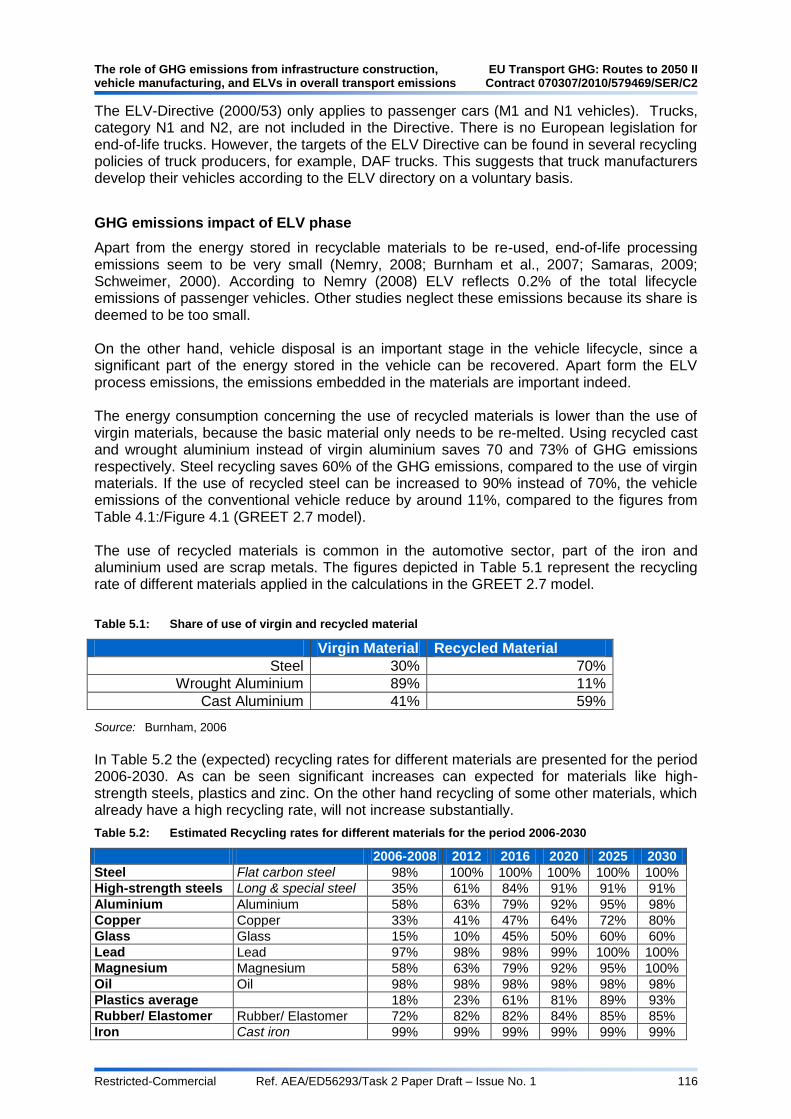
The role of GHG emissions from infrastructure construction, EU Transport GHG: Routes to 2050 II vehicle manufacturing, and ELVs in overall transport emissions Contract 070307/2010/579469/SER/C2
Restricted-Commercial Ref. AEA/ED56293/Task 2 Paper Draft – Issue No. 1 116
The ELV-Directive (2000/53) only applies to passenger cars (M1 and N1 vehicles). Trucks, category N1 and N2, are not included in the Directive. There is no European legislation for end-of-life trucks. However, the targets of the ELV Directive can be found in several recycling policies of truck producers, for example, DAF trucks. This suggests that truck manufacturers develop their vehicles according to the ELV directory on a voluntary basis.
GHG emissions impact of ELV phase
Apart from the energy stored in recyclable materials to be re-used, end-of-life processing emissions seem to be very small (Nemry, 2008; Burnham et al., 2007; Samaras, 2009; Schweimer, 2000). According to Nemry (2008) ELV reflects 0.2% of the total lifecycle emissions of passenger vehicles. Other studies neglect these emissions because its share is deemed to be too small. On the other hand, vehicle disposal is an important stage in the vehicle lifecycle, since a significant part of the energy stored in the vehicle can be recovered. Apart form the ELV process emissions, the emissions embedded in the materials are important indeed. The energy consumption concerning the use of recycled materials is lower than the use of virgin materials, because the basic material only needs to be re-melted. Using recycled cast and wrought aluminium instead of virgin aluminium saves 70 and 73% of GHG emissions respectively. Steel recycling saves 60% of the GHG emissions, compared to the use of virgin materials. If the use of recycled steel can be increased to 90% instead of 70%, the vehicle emissions of the conventional vehicle reduce by around 11%, compared to the figures from Table 4.1:/Figure 4.1 (GREET 2.7 model). The use of recycled materials is common in the automotive sector, part of the iron and aluminium used are scrap metals. The figures depicted in Table 5.1 represent the recycling rate of different materials applied in the calculations in the GREET 2.7 model.
Table 5.1: Share of use of virgin and recycled material
Virgin Material Recycled Material
Steel 30% 70%
Wrought Aluminium 89% 11%
Cast Aluminium 41% 59%
Source: Burnham, 2006
In Table 5.2 the (expected) recycling rates for different materials are presented for the period 2006-2030. As can be seen significant increases can expected for materials like high-strength steels, plastics and zinc. On the other hand recycling of some other materials, which already have a high recycling rate, will not increase substantially.
Table 5.2: Estimated Recycling rates for different materials for the period 2006-2030
2006-2008 2012 2016 2020 2025 2030
Steel Flat carbon steel 98% 100% 100% 100% 100% 100%
High-strength steels Long & special steel 35% 61% 84% 91% 91% 91%
Aluminium Aluminium 58% 63% 79% 92% 95% 98%
Copper Copper 33% 41% 47% 64% 72% 80%
Glass Glass 15% 10% 45% 50% 60% 60%
Lead Lead 97% 98% 98% 99% 100% 100%
Magnesium Magnesium 58% 63% 79% 92% 95% 100%
Oil Oil 98% 98% 98% 98% 98% 98%
Plastics average 18% 23% 61% 81% 89% 93%
Rubber/ Elastomer Rubber/ Elastomer 72% 82% 82% 84% 85% 85%
Iron Cast iron 99% 99% 99% 99% 99% 99%

EU Transport GHG: Routes to 2050 II The role of GHG emissions from infrastructure construction, Contract 070307/2010/579469/SER/C2 vehicle manufacturing, and ELVs in overall transport emissions
Restricted-Commercial Ref. AEA/ED56293/Task 2 Paper Draft – Issue No. 1 117
2006-2008 2012 2016 2020 2025 2030
Textile Textile 45% 45% 50% 60% 70% 80%
Zinc Zinc 30% 38% 45% 60% 75% 90%
Other fluids Other fluids 70% 70% 80% 99% 99% 99%
Other metals Other metals 40% 55% 65% 65% 65% 70%
Source: TREMOVE
Future prospects
The 2015 standards for recycling can be observed as high with a recycling rate of 85% and a recovery rate of 95%. This implies that the potential of recycling of additional materials is limited. Recycling of the plastic components does not significantly change the GHG impacts, compared to recovery (Schmidt, Dahlqvist et al., 2004). An Austrian study concludes that optimisation options are limited and expensive (Neubacher, 2005). DAF Trucks has stated on its website that their trucks are designed to be recycled for 93% (and recovered for 96%) (DAF, 2011) However, there is no guarantee those recycling rates are met by the disposal of trucks. It is recommended to investigate the possibilities to include trucks in the ELV-Directive in the future in order to guarantee the recycling rates from which car producers state that it is feasible. Battery recycling is an issue that will need attention in the next decades, since recycling will be an important pre-requisite preventing an increase in ELV emissions. This is not only important from a climate point of view, but also from a pollution point of view (acidification). The ELV Directive covers all passenger vehicles including batteries, but particular attention may still be needed for the batteries.
5.1.2 References
AEA (2007) Hybrid Electric and Battery Electric Vehicles, Technology, Costs and benefits, November 2007 A. Burnham, M. Wang, and Y. Wu, (2006) Development and Applications of GREET 2.7 - The Transportation Vehicle-Cycle Model, Energy Systems Division, Argonne National Laboratory. 2006. DAF (2011) „Levenscyclus: Drie fasen: productie, gebruik en afdanking‟ Last retrieved on April 7, 2011 http://www.daf.com/NL/About-DAF/Environment/Pages/Product-lifecycle.aspx Eurostat (2011) „End-of-life vehicles‟ Last retrieved on April 8, 2011 http://epp.eurostat.ec.europa.eu/portal/page/portal/waste/data/wastestreams/elvs Nemry (2008) Environmental Improvement of Passenger Cars (IMPRO-car), Françoise NEMRY, Guillaume LEDUC, Ignazio MONGELLI, Andreas UIHLEIN Neubacher, F (2005) Evaluation of the Measures and Targets of the Austrian End-of-Life Vehicles Ordinance with regard to the Implementation of the Directive 2000/53/EC, VDI MSc Process Engineering, M.S. Technology & Policy (M.I.T.) OVAM (2008) H. De Baets, „Validation of the recycling percentages for end-of-life vehicles at shredder companies and flotation units‟

The role of GHG emissions from infrastructure construction, EU Transport GHG: Routes to 2050 II vehicle manufacturing, and ELVs in overall transport emissions Contract 070307/2010/579469/SER/C2
Restricted-Commercial Ref. AEA/ED56293/Task 2 Paper Draft – Issue No. 1 118
Samaras, C and Meisterling, K (2009) Life Cycle Assessment of Greenhouse Gas Emissions from Plug-in Hybrid Vehicles: Implications for Policy, Environ. Sci. Technol. 2009. W. Schmidt, E. Dahlqvist, M. Finkbeiner, S. Krinke, S. Lazzari, D. Oschmann, S. Pichon and C. Thiel (2004) „Life Cycle Assessment of Lightweight and End-of-Life Scenarios for Generic Compact Class Passenger Vehicles‟ In: International Journal of Life Cycle Assesment 9 (6) 405 – 416 (2004) Schweimer, G (2000) Life Cycle Inventory for the Golf A4, Research, Environment and Transport, Volkswagen AG, Wolfsburg, Marcel Levin, Center of Environmental Systems Research, University of Kassel Lane (2006) Lifecycle assessment of vehicle fuels and technologies. s.l. : A study carried out for the London Borough of Camden. SMMT (2009) Tenth annual sustainability report 1999 – 2008, The Society of Motor Manufacturers and Traders, 2008, Londen, United Kingdom Pehnt (2003) Assessing Future Energy and Transport Systems: The Case of Fuel Cells Part 2: Environmental Performance, Martin Pehnt, Institute for Energy and Environmental Research Heidelberg (Ifeu), in : Environmental Performance [Int J LCA 8 (6) 365 – 378 (2003)]
5.2 Rail
5.2.1 Summary of information from the literature
Little information has been identified in the literature specifically on the end-of-life phase of rail rolling stock, although this phase is often accounted for within broader analyses, such as previously presented in Figure 4.15. Although there is very little information available in the literature, one study by KATO (2005) reports the recycling of the Japanese Shinkansen trains is over 90%. No comparable information has been identified for European heavy rail rolling stock, however information from Siemens (2011) suggests that 68% of the Oslo metro railcar is expected to be recycled. It is anticipated that a higher proportion of heavy rail rolling stock is recyclable due to their higher proportional content of steel and aluminium (see Figure 4.14). As already discussed in the earlier section on vehicle manufacturing (section 4.2), the specific methodology for accounting for recycling has a significant bearing on the analysis. TBC after focus group meeting…
5.2.2 Identification of gaps – focus group
Gaps in the literature which the focus group may be able to add to:
Disposal methods – energy use and emissions from the process of recycling parts
compared with disposal of them. May be very different for different materials
End of life rail rolling stock legislation or regulation??
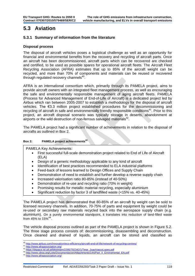
EU Transport GHG: Routes to 2050 II The role of GHG emissions from infrastructure construction, Contract 070307/2010/579469/SER/C2 vehicle manufacturing, and ELVs in overall transport emissions
Restricted-Commercial Ref. AEA/ED56293/Task 2 Paper Draft – Issue No. 1 119
5.3 Aviation
5.3.1 Summary of information from the literature
Disposal process
The disposal of aircraft vehicles poses a logistical challenge as well as an opportunity for financial and environmental benefits from the recovery and recycling of aircraft parts. Once an aircraft has been decommissioned, aircraft parts which can be recovered are checked and certified, to be used as possible spares for operational aircraft fleets. The Aircraft Fleet Recycling Association (AFRA) estimates that up to 85% of the aircraft weight can be recycled, and more than 70% of components and materials can be reused or recovered through regulated recovery channels40. AFRA is an international consortium which, primarily through its PAMELA project, aims to provide aircraft owners with an integrated fleet management process, as well as encouraging the safe and environmentally responsible management of aging aircraft fleets. PAMELA (Process for Advanced Management of End-of-Life of Aircraft) is a dedicated project led by Airbus which ran between 2005-2007 to establish a methodology for the disposal of aircraft vehicles. The €3.3 million project established procedures for the decommissioning and recycling of aircraft in safe and environmentally friendly responsible conditions41. Prior to this project, an aircraft disposal scenario was typically storage in deserts, abandonment at airports or the wild destruction of non-ferrous salvaged materials42. The PAMELA project had a significant number of achievements in relation to the disposal of aircrafts as outlined in Box 2.
Box 2: PAMELA project achievements43
The PAMELA project has demonstrated that 80-85% of an aircraft by weight can be sold to licensed recovery channels. In addition, 70-75% of parts and equipment by weight could be re-used or secondary raw materials recycled back into the aerospace supply chain (e.g. aluminium). On a purely environmental standpoint, it translates into reduction of land-filled waste
from 45% to 15%44.
The vehicle disposal process outlined as part of the PAMELA project is shown in Figure 5.2. The three stage process consists of: decommissioning, disassembling and deconstruction. Once cleaned and drained of liquids, an aircraft can be stored and classified as
40
http://www.airbus.com/innovation/eco-efficiency/aircraft-end-of-life/network-of-recycling-centres/ 41
http://www.afraassociation.org/ 42
https://dspace.ist.utl.pt/bitstream/2295/792342/1/Tese_JoaoVascoLopes.pdf 43
http://www.obsa.org/Lists/Documentacion/Attachments/144/Part_II_Enviromental_EN.pdf 44
http://www.afraassociation.org/
PAMELA Key Achievements:
First successful full-scale demonstration project related to End of Life of Aircraft (ELA)
Design of a generic methodology applicable to any kind of aircraft
Identification of best practices recommended to ELA industrial platforms
Feed-back of lessons learned to Design Offices and Supply Chain
Demonstration of need to establish and further develop a reverse supply chain
Increased valorisation ratio 80-85% (instead of 40-50%)
Demonstration of re-use and recycling ratio (70% in weight)
Promising results for metallic material recycling, especially aluminium
Significant reduction by factor 3 of landfilled waste (<15% vs. 40-45%)

The role of GHG emissions from infrastructure construction, EU Transport GHG: Routes to 2050 II vehicle manufacturing, and ELVs in overall transport emissions Contract 070307/2010/579469/SER/C2
Restricted-Commercial Ref. AEA/ED56293/Task 2 Paper Draft – Issue No. 1 120
decommissioned. The second stage, disassembly, is the activities required to remove all the valuable components from an aircraft, which can be re-used in another aircraft45. This stage will include the removal of high value components, such as engines which will have a high monetary value when sold back into service. Once this stage has been completed, an aircraft can be dismantled, which involves aiming to achieve as a high a recycling rate as possible by separating recyclable metals and plastics from non-recyclable materials.
Figure 5.2: Key Steps in the PAMELA Process
Source: http://www.obsa.org/Lists/Documentacion/Attachments/144/Part_II_Enviromental_EN.pdf
Dismantling facilities
The PAMELA project was followed by a second phase under the TARMAC-AEROSAVE (Tarbes Advanced Recycling and Maintenance Aircraft Company), the first industrial company to manage end-of-life aircraft46. The joint venture between Airbus and waste management company SITA France offers storage, maintenance and „smart dismantling‟ of aircraft47. A TARMAC-Aerosave end-of-life centre in Tarbes, France benefits from the dismantling and recycling practice lessons learned from PAMELA. A US facility which offers end-of-life management solutions is the Aerospace Maintenance and Regeneration Group (AMARG), also known as The Boneyard. This United States Air Force aircraft and missile storage and maintenance facility is located on Davis-Monthan Air Force Base in Tuscon, Arizona. Taking care of more than 4,400 aircraft, the site is the sole repository of out-of-service aircraft from all branches of the US government48. There are four categories of aircraft storage for planes at AMARG:
Long Term - Aircraft are kept intact for future use
Parts Reclamation - Aircraft are kept, picked apart and used for spare parts
Flying Hold - Aircraft are kept intact for shorter stays than Long Term
Excess of US Department of Defence - Aircraft are sold off whole or in parts
45
http://www.aels.nl/en/disassembly_and_dismantling/definitions 46
http://www.obsa.org/Lists/Documentacion/Attachments/144/Part_II_Enviromental_EN.pdf 47
http://www.tarmacaerosave.aero/dismantling.html 48
US Air Force (2008) Aerospace Maintenance and Regeneration Group. Davis-Monthan Air Force Base. Available at: http://www.dm.af.mil/library/factsheets/factsheet.asp?id=4383

EU Transport GHG: Routes to 2050 II The role of GHG emissions from infrastructure construction, Contract 070307/2010/579469/SER/C2 vehicle manufacturing, and ELVs in overall transport emissions
Restricted-Commercial Ref. AEA/ED56293/Task 2 Paper Draft – Issue No. 1 121
At the 2,600 acre AMARG site, there is an inventory of more than 4,200 aircraft, 40 aerospace vehicles and 350,000 line items of production tooling. Part of this inventory is shown in Figure 5.3. In 2005, the Commodities Division reclaimed and shipped worldwide 19,194 parts valued at almost $568 million. The financial benefits of the recovery and dismantling at the AMRG site are understood more clearly than the emissions saved. AMARG estimates that for every US$1 the federal government spends operating the facility, it saves or produces US$11 from harvesting spare parts and selling off inventory49.
Figure 5.3: Ariel view of the AMARG aircraft graveyard in Tucson, Arizona, USA.
Source: http://www.artificialowl.net/2008/05/amarc-biggest-plane-graveyard-tucson.html
Recyclable materials & associated emissions
As discussed, using the PAMELA methodology, up to 85% of the weight of an aircraft can be recycled, and more than 70% of components and materials can be reused or recovered through regulated recovery channels. Aluminium is the primary material used in the construction of aircrafts, contributing to the majority of the weight in both the fuselage and wings of aircrafts. Figure 5.4 provides an end-of-life aircraft scenario for an A330-200 under the PAMELA project. In total, 71,898Kg of the aircraft has recyclable value at the end of life stage, equating to 68% of the total aircraft weight. Of this 68%, 43% is purely aluminium which can be recycled, representing the largest recyclable material from the vehicle. Airbus estimates that the recycling process for aluminium consumes 90% less energy than its initial primary production50. Figure 5.4 shows that from a PAMELA project scenario, composites from aircraft fuselage, stabilisers and engine structures have no valuable weight based on a typical disposal scenario of 50% incineration : 50% landfill. Composites from the wings of the aircraft under this scenario are similarly incinerated and landfilled at a 50/50 ratio.
49
US Air Force (2008) Aerospace Maintenance and Regeneration Group. Davis-Monthan Air Force Base. Available at: http://www.dm.af.mil/library/factsheets/factsheet.asp?id=4383 50
http://www.airbus.com/innovation/eco-efficiency/aircraft-end-of-life/network-of-recycling-centres/

The role of GHG emissions from infrastructure construction, EU Transport GHG: Routes to 2050 II vehicle manufacturing, and ELVs in overall transport emissions Contract 070307/2010/579469/SER/C2
Restricted-Commercial Ref. AEA/ED56293/Task 2 Paper Draft – Issue No. 1 122
Figure 5.4: End-of-life scenario for the A330-200 aircraft (PAMELA)
Source: https://dspace.ist.utl.pt/bitstream/2295/792342/1/Tese_JoaoVascoLopes.pdf
In the future, the recycling of composites has potential to increase the GHG emissions savings from the end of life aircraft stage. Advanced composites are not widely recycled at present but instead are either sent to landfill or incinerated at high temperatures. This process gives rise to hazardous air pollutants and wastes whilst reducing the overall aircraft recyclable rates51. A strategic goal to boost the use of lightweight composites has been set by the US Department of Defence to achieve a 100-fold increase in use in the next 30 years. The next generation of civil aircraft are likely to employ optimised composite structures with complex shape designs and equally sophisticated manufacturing processes. An Omega study by the University of Sheffield52 found that
Figure 5.5: Comparison of airborne emissions of carbon dioxide (a) production and disposal only, and (b) after use in the aircraft.
51
http://www.omega.mmu.ac.uk/could-composites-hold-a-key-to-improved-emissions-performance.htm 52
http://www.omega.mmu.ac.uk/Downloads/Final-Reports/34%20Final%20Report%20Composite%20materials.pdf

EU Transport GHG: Routes to 2050 II The role of GHG emissions from infrastructure construction, Contract 070307/2010/579469/SER/C2 vehicle manufacturing, and ELVs in overall transport emissions
Restricted-Commercial Ref. AEA/ED56293/Task 2 Paper Draft – Issue No. 1 123
Figure 5.4 compares the emissions of carbon dioxide produced by aluminium alloy, GLARE53 and carbon fibre epoxy resin composites. Graph (a) accounts for production and disposal only, showing that aluminium produces less carbon dioxide than alternative composite materials. However, when including the operational stage in graph (b), the heavier aluminium overtakes the lighter composite materials to produce more carbon dioxide overall.
5.3.2 Identification of gaps – focus group
Gaps in the literature which the focus group may be able to add to:
Disposal methods – energy use and emissions from the process of recycling parts
compared with disposal of them. May be very different for different materials.
End of life aviation legislation.
5.4 Shipping
5.4.1 Summary of information from the literature
On a global scale, for vessels of different sizes it is not very well known which dismantling routes are followed to which extent. What is most important from the perspective of greenhouse gas emissions, is the extent to which steel is being recycled. Given the positive economic value it is expected that this extent is high, irrespective of the physical final destination of the ship. The CO2 emissions related to the actual dismantling process and treatment of other materials is expected to be of minor importance. Some CO2 emission will result from (controlled or uncontrolled) incineration of combustible materials like plastics and hydraulic oil. Ship scrapping products can be divided into a number of categories:
Useable materials, equipment and machinery;
Repairable engines, machinery, and equipment;
Recycled materials, equipment,, and engines; and
Waste. The ship scrapping process results in the following:
Ferrous materials: steel plates and sections, pipes stiffened panels, cast iron, cast steel etc;
Non-ferrous materials: copper, brass, bronze, aluminium, zinc etc;
Non-metalic materials;
Equipment: electrical, navigation, electronic, communication etc; and
Machinery: cranes, winches, motors, pumps etc, and engines: main and auxiliary (Sharma, 2005).
Steel recycling is credited for the fact that keeping the steel in the loop avoids primary steel production elsewhere. Assuming a steel recycling rate of 95%, the disposal of a vessel leads to a CO2 „credit‟ of approximately 2% of its life cycle emission. This is based on the approach introduced in section 4.4. All in all, the contribution of production plus disposal to the ship‟s life cycle CO2 emission is expected to be in the order of 1%. Energy efficiency of ship scrapping could be improved through the development of appropriate management systems. Such systems may include:
53
GLARE is a hybrid GLAss-REinforced fibre metal laminate

The role of GHG emissions from infrastructure construction, EU Transport GHG: Routes to 2050 II vehicle manufacturing, and ELVs in overall transport emissions Contract 070307/2010/579469/SER/C2
Restricted-Commercial Ref. AEA/ED56293/Task 2 Paper Draft – Issue No. 1 124
Maximising reuse, recover and repair of materials, fittings, equipment, machinery, engines etc;
Minimising wastes and recycled materials, machinery, equipment, engines etc; and
Minimising energy consumption and the negative environmental impacts (Sharma, 2005).
5.4.2 References
Sharma, M.A (2005) Life cycle assessment of ships, Maritime transportation and exploration of ocean and coastal resources, Taylor and Francis Group, London. http://teaching.alexeng.edu.eg/Naval/MShama/LCASO-215.pdf
5.4.3 Identification of gaps – focus group
Gaps in the literature which the focus group may be able to add to:
Disposal methods – energy use and emissions from the process of recycling parts
compared with disposal of them. May be very different for different materials.
End of life shipping legislation.
EU Transport GHG: Routes to 2050 II The role of GHG emissions from infrastructure construction, Contract 070307/2010/579469/SER/C2 vehicle manufacturing, and ELVs in overall transport emissions
Restricted-Commercial Ref. AEA/ED56293/Task 2 Paper Draft – Issue No. 1 125
6 Reaching Optimal Solutions
Objectives: The purpose of this sub-task was to provide:
A summary comparison of current and (possible) future relative significance of emission components versus vehicle in-use emissions by mode of transport;
An assessment of the possible impacts of including emissions from infrastructure and vehicle production and disposal in the relative performance of different scenario options for reducing GHG emissions in the long term to 2050.
Summary of Main Findings
To be completed for final draft after focus group meeting on 4th May 2011 later in the project
6.1 Modal comparisons
To be completed for final draft after focus group meeting on 4th May 2011 later in the project Will include summary example comparison of current and (possible) future relative significance of emission components vs vehicle in-use emissions by mode.
6.2 Comparison of alternate scenarios
To be completed for final draft after focus group meeting on 4th May 2011 later in the project Will include comparisons based on scenarios to be developed later in the project on alternative routes to 60% reduction in transport GHG by 2050

The role of GHG emissions from infrastructure construction, EU Transport GHG: Routes to 2050 II vehicle manufacturing, and ELVs in overall transport emissions Contract 070307/2010/579469/SER/C2
Restricted-Commercial Ref. AEA/ED56293/Task 2 Paper Draft – Issue No. 1 126
7 Summary of Key Findings and Conclusions
To be completed for final draft after focus group meeting on 4th May 2011 later in the project once all other sections are complete. Will include possible options to reduce/minimise emissions


The Gemini Building Fermi Avenue Harwell International Business Centre Didcot Oxfordshire OX11 0QR
Tel: 0870 190 1900 Fax: 0870 190 6318
www.aeat.co.uk