The Risk and Return of Impact Investing Funds

Jessica Jeffers∗ Tianshu Lyu† Kelly Posenau‡

November 2021

Abstract

We provide the first analysis of the risk exposure and consequent risk-adjusted performance of

impact investing funds, private market funds with dual financial and social goals. We introduce a

new dataset of impact fund cash flows constructed from financial statements. When accounting for

market risk exposure, impact funds underperform the market, though not more so that comparable

private market strategies. We exploit known distortions in measures of VC performance to char-

acterize the risk profile of impact funds. Impact funds have substantially lower market beta than

VC funds, contradicting the idea of sustainability as a “luxury good.” We find that impact fund

cash flows do not exhibit positive correlation with a public market sustainability factor, consistent

with the idea that private and public market sustainability strategies capture distinct exposures.

The authors thank Shawn Cole, Shaun Davies, Peter Dunbar, Arpit Gupta, Wendy Hu, Arthur Korteweg, StefanNagel, Veronika Pool, Tristan Reed, Morten Sorensen, and conference and seminar participants where we have presentedthis paper. This work is supported by the David G. Booth Endowment and the Fama-Miller Center at the Universityof Chicago Booth School of Business. We are also grateful to IPC/PERC for access to Burgiss data, and to the ImpactFinance Research Consortium and funds participating in its Impact Finance Database.∗University of Chicago, Booth: jessica.jeffers@chicagobooth.edu†Yale University, SOM: tianshu.lyu@yale.edu‡University of Chicago, Booth: kposenau@chicagobooth.edu

1 Introduction

As major societal problems like climate change and inequality grow, investors and the public have

become increasingly interested in whether financial markets can be harnessed to help address these

issues. Industry participation in sustainable finance and responsible investing has exploded in recent

years, with global sustainable investing assets amounting to $30.7 trillion in 2018, a 34 percent increase

in two years (GSIA, 2018). While social and environmental responsibility are often debated in the

context of public markets, private markets are uniquely suited to address these challenges because of

their dominance in early-stage and growth transactions. At these early stages in companies’ lifespans,

capital providers exert more influence on both deal sourcing and governance than what they would be

able to achieve in public markets (Phalippou, 2017; Gompers et al., 2020).

Impact investing is the practice of using private market strategies to target both financial returns

and a social or environmental goal. Although impact investing is a rapidly growing asset class, with

$715 billion in assets under management globally, relatively little is known about the financial proper-

ties of this approach (Hand et al., 2020; Burton et al., 2021). In particular, to the best of our knowledge

no work has addressed the riskiness of impact investing or its financial performance adjusted for market

risk exposure.1

This paper fills a gap in the literature by characterizing the risk-adjusted return of impact investing

and its risk properties relative to other strategies. Three reasons motivate us. First, establishing risk

and return properties is a critical component of understanding the feasibility and future of impact

investing—even (perhaps especially) if impact investing is not a strategy that maximizes returns.

If impact is concessionary, it is essential to describe the magnitude of the potential risk-adjusted

concession in order to understand who will be able or willing to participate in these strategies. Likewise,

characterizing the riskiness of impact investing can also illuminate how impact investing fits into

existing portfolios.2

Second but equally important, a large debate over the returns of impact investing reflects divergent

theories of the market. Under standard assumptions (perfect and complete capital markets, rational

and informed investors), constrained strategies like impact investing must have lower risk-adjusted

returns than unconstrained strategies (Brest et al., 2018; Barber et al., 2021). If these standard1Barber et al. (2021) take an important first step in understanding the performance of impact investing by bench-

marking impact fund performance using IRRs and multiples. However, without fund cash flows, they are unable tospeak to the risk exposure or risk-adjusted performance of impact funds. Similarly, Cole et al. (2020) abstract from riskexposures in their analysis of long-run returns to impact investing.

2Some have argued that impact investing is only meaningful when it has additionality, and that impact investmentsshould be motivated by a moral imperative rather than a financial one (e.g. Phalippou (2017)). We do not disagree withthese positions. Our focus in this paper is descriptive rather than prescriptive.

1

assumptions fail, however, the inequality need not hold. This is in line with recent work by Cole et al.

(2020), which finds that markets are imperfectly integrated and that impact investing extracts value

from this market friction, leading to potentially higher returns than unconstrained strategies. Risk is

a critical part of this debate: concessionary absolute returns may still be consistent with a profitable

strategy if the strategy hedges risks. Profitable risk-adjusted returns for a constrained strategy would

provide evidence in favor of the violation of standard market assumptions.

Third, the risk profile of impact investing sheds light on different models about the risk of sustain-

able and green assets. The covariance of impact investing with the market is in theory ambiguous. On

one hand, Bansal et al. (2018) document that socially responsible investing (SRI) in public markets

is highly pro-cyclical. Extending this theory to private markets, we might expect the market beta

of impact investing to be high, and higher than comparable nonimpact private strategies.3 On the

other hand, Nofsinger and Varma (2014) and Pástor and Vorsatz (2020) find evidence that sustainable

mutual funds outperform during market crises. Recent work by Gibson et al. (2019) and Wang and

Sargis (2020) suggests that ESG investing in public markets can reduce portfolio risk. This counter-

cyclical view of sustainable investing would correspond to a lower market beta for impact relative to

nonimpact strategies. There are additional risk factors that an impact investor may be interested in

hedging. For example, evidence indicates that climate risk is a growing concern for investors (Krueger

et al., 2020), and that it may be mispriced in financial markets (Andersson et al., 2016; Engle et al.,

2020). By focusing on solutions to climate and other risks, impact investing may serve as a hedge for

downside risks, implying a potentially lower beta than comparable nonimpact strategies.

Private market funds in general, and impact investing funds in particular, present several challenges

for studying risk and return. Infrequent and highly skewed payoffs make it difficult to use traditional

linear factor modeling techniques. Small sample sizes and young funds exacerbate these problems. To

address these issues in the VC literature, Korteweg and Nagel (2016) develop the Generalized Public

Market Equivalent (GPME), an extension of the Public Market Equivalent (PME) first proposed by

Kaplan and Schoar (2005). As Korteweg and Nagel (2016) show, although the PME has many useful

features for assessing the performance of venture capital, it assumes a restricted market equity premium

and risk-free rate. As a result, the PME systematically overestimates the performance of high-beta

assets in times of rising public equity markets. This bias grows with the asset’s market beta.

Our key insight is to leverage these known biases in performance measures to back out the risk

properties of impact investing. Given that our sample time period is one of rising public equity markets,3Previous work has found evidence of a sizeable market beta for venture capital (VC) investing strategies. For

example, Cochrane (2005) finds a beta of 1.9.

2

the distance between PME and GPME (the “PME wedge”) informs us about the relative market beta

of the underlying asset. If impact investing is a high-beta asset, then its PME wedge will be positive;

if it is a low-beta asset (beta less than one), the PME wedge will be negative. Moreover, artificially

levering up the strategy, and thus amplifying its beta, should amplify the PME wedge: if unlevered

beta is positive, the PME wedge will increase. This reasoning extends to relative properties across

strategies. For example, if impact investing has a higher (lower) beta than VC, its PME wedge will be

greater (smaller) than the PME wedge of VC.

The same logic can be applied to other factor covariances. We derive the relative covariance of

impact investing with different public factors, such as a sustainability index, by estimating PME and

GPME with the alternative factor and comparing the new PME wedge across impact and nonimpact

strategies. Finally, we extend our model to multiple factors, and test whether impact investing cash

flows are spanned by a combination of the market and other factors.

We use two sources of data for impact investing cash flows, both stemming from work done as

part of the Impact Finance Research Consortium (IFRC), a cross-school collaboration to build data

on impact investing funds. First, as part of the IFRC effort, we collect annual and quarterly financial

statements directly from impact funds and manually convert them into a standardized database cover-

ing contributions and distributions net of fees, as well as net asset value (NAV), among other variables.

Our aim is to eventually make the resulting Impact Finance Database (IFD) available for researchers.

As of this writing, the IFD contains cash flows for 62 funds from 1999 through 2017. After restricting

analysis to funds targeting market-rate returns and with sufficient data, we are left with 48 distinct

funds. Second, we leverage the comprehensive list of past and existing impact funds created by the

IFRC, and search for these funds in Preqin. We find cash flows for an additional 46 impact funds,

bringing our total sample to 94 funds.

We construct comparison fund groups using fund cash flows from Preqin, and in the appendix

include comparisons to Burgiss as well. Benchmark comparison groups serve two purposes. First,

benchmarking to a well-understood asset class helps us understand performance in an established

context. For this purpose, our first comparison group is the universe of US-based VC funds over the

same time period as our sample. We choose VC because it is the asset class most representative

of impact funds overall (Geczy et al., 2020), and its risk and return properties have been studied

extensively (Korteweg, 2019). The second purpose of benchmarking is to try to isolate the influence of

the impact component. As a second comparison group, we match each impact fund in our sample to

a Preqin fund with the same vintage, asset type, and as close as possible on size. Perfectly controlling

for everything outside impact is not possible, but this smaller benchmark helps us to address the effect

3

of characteristics known to influence risk exposure.

We find that after properly accounting for risk exposure and the rising market equity premium,

impact funds underperform the public market by $0.45 per $1 invested over the 1999-2017 time period.

Market risk exposure alone cannot explain the low returns of impact investing. At the same time, we

find VC underperforms public benchmarks by an average $0.44 per $1 invested over the same time

period. A value-weighted portfolio that goes long $1 in VC and short $1 in impact funds has a negative

market risk-adjusted return of −$0.15. The equal-weighted long-short portfolio has a positive market

risk-adjusted return of $0.02. Matched funds perform somewhat better, with a loss of “only” $0.31

per $1 invested. A portfolio long in matched funds and short impact yields a value-weighted return of

−$0.05 and an equal-weighted return of $0.04, neither statistically different from zero. Our results are

thus consistent with previous findings that private market strategies have generally underperformed

public markets in the past two decades. We show this pattern extends to impact funds, but not more

so than comparable private market strategies.

Our findings provide a new perspective for the debate on financial performance and market com-

pleteness. On one hand, we confirm that the constrained impact strategy is concessionary relative to

the risk-return frontier that can be achieved in public markets. On the other hand, impact returns

are not clearly concessionary relative to private market benchmarks after accounting for systematic

risk. Since VC participants (for example) could in principle invest in the same deals as impact funds,

this points to the failure of one or more assumptions in private markets. Cole et al. (2020) argue that

imperfect integration of international capital markets enable profitable impact investing strategies.

Other possibilities include information barriers, investor biases, and distortions to competition in both

capital and product markets.

Our second main result is that impact investing is substantially less sensitive to movements in

public equity markets than VC, and to a lesser extent, than matched funds. The PME overestimates

impact performance relative to the GPME in our time period, consistent with a market beta greater

than one.4 When we artificially lever up our impact fund cash flows, the PME wedge increases, also

consistent with a positive beta that grows as the strategy is levered up. However, this wedge grows

more slowly for impact funds than for VC and matched funds. We can reject that impact beta is

close to VC beta. A portfolio that goes long $1 in VC and short $1 in impact still has a positive

beta, indicating greater market risk exposure for VC than for impact. The difference with matched

funds is lower, but still consistent with a particularly low beta for impact. Overall, impact is not as

pro-cyclical as we would expect for a “luxury good”, or at least not as much as VC. Instead, adding4This statement holds true in times of rising market equity premia, which we show is the case for our sample period.

4

impact investments to a private market investor’s VC portfolio reduces overall market risk exposure.

Third, impact investing captures distinctive risk exposures. While impact fund returns are not

spanned by the market and a small growth factor, we cannot reject that a two-factor model with the

market and a public market sustainability index does not span impact returns. In contrast, neither of

these multifactor models span VC cash flows better than the single-factor market risk model, in the

sense that the negative magnitude of absolute returns cannot be explained by exposure to these risk

factors. We also consider the model of an investor who cares about sustainability, and invests only

in the public market sustainability index. In this setting, impact underperforms the sustainability

benchmark, while both benchmarks outperform. This indicates that if investors are targeting exposure

to a public sustainability factor, then impact investing is not a profitable means to gain this exposure.

Our work contributes to the broader understanding of SRI and environmental, social, and gover-

nance (ESG) factors. Most existing work has focused on public markets, exploring investor taste for

“green” strategies (Hartzmark and Sussman, 2019; Krueger et al., 2020; Pastor et al., 2019; Fama and

French, 2007) and the pricing of ESG factors (Ilhan et al., 2021; Bansal et al., 2018). Renneboog et al.

(2008) provide an overview of SRI in mutual funds. We extend this work to private markets, which

present a different set of challenges and opportunities for sustainability-minded investors. Companies

seeking capital in the impact investing market are typically orders of magnitude smaller than public

companies, with completely different expected growth paths and risk considerations. The potential for

impact is also distinct from public market investments. Investors, via funds, have substantially more

influence over the development of portfolio companies than they would in public companies.

Data limitations have kept the literature on impact investing sparse, but this paper joins a few

others in the burgeoning literature on impact investing. On the descriptive side, Burton et al. (2021)

introduce a new database on investor and firm characteristics in impact investing, and provide essential

statistics to understand this emerging space; Geczy et al. (2020) detail the contracting and governance

practices of impact investing funds.5 On the theory side, Chowdhry et al. (2019), Oehmke and Opp

(2020) and Green and Roth (2020) propose models for the existence and usefulness of impact investing.

Two other papers study the financial performance of private impact investing funds: Barber et al.

(2021) use a willingness-to-pay model to show that investors accept 2.5%-3.7% lower internal rates

of return (IRRs) for impact funds, and Cole et al. (2020) find that a large impact investor’s long-

run returns outperformed the market by 15% over nearly seven decades of investing activity. We

provide a new perspective to these two papers by explicitly addressing the risk exposure of impact5Both projects are related to the Impact Finance Database introduced in this paper: Geczy et al. (2020) leverage the

contract data portion of the IFD, and several of the individuals involved in the Impact Investment Database describedin Burton et al. (2021) also contribute actively to the IFRC.

5

cash flows.In our sample, impact underperforms relative to public markets, but not more so than

comparable strategies after accounting for market risk exposure. An advantage of our data is that we

can differentiate impact funds that are explicitly concessionary from funds that state their intention

to achieve market-rate returns. Our current results pertain to the latter only.

Last, this paper contributes to a rich asset pricing literature on the risk and return of PE and

VC cash flows, starting with Cochrane (2005) and Korteweg and Sorensen (2010). More recently,

Ang et al. (2018) estimate a PE-specific return series using a Bayesian approach and assuming a

linear factor structure. Gupta and Van Nieuwerburgh (2019) propose a new method to risk-adjust PE

returns and estimate factor risk exposures for each cash flow horizon. We build heavily on the GPME

approach introduced by Korteweg and Nagel (2016), leveraging the distortions that they document to

back out the risk properties of impact and VC funds. This approach allows us to directly compare

VC and impact funds in an intuitive way. A key difference between this method annd Gupta and

Van Nieuwerburgh (2019) is that the latter uses expectations of stochastic discount factors (SDFs)

from dividend strip prices, while we rely on the realized SDF.

The remainder of the paper proceeds as follows. We describe our data in Section 2 and our approach

and predictions in Section 3. In Section 4, we show results relative to market exposure, and in Section 5

we introduce other factors. Section 6 concludes.

2 Data

One of the challenges in studying impact investing is the lack of data. We overcome this challenge

by creating a new dataset of impact investing cash flows from new and preexisting data sources. This

section explains our data sources and construction. We start with the sample of impact funds, then

describe benchmark VC and matched funds, followed by summary statistics for all three samples. We

also describe the data for the public market replicating portfolios used in the GPME approach, which

we further describe in Section 3.2.

2.1 Impact Investing Funds

This paper uses a new data source, the Impact Finance Database (IFD), that we developed as

part of the IFRC, a collaboration across the Wharton School of Business, Harvard Business School,

and the University of Chicago’s Booth School of Business. The IFD encompasses multiple datasets,

covering four key aspects of impact funds: their financial cash flows, impact reports, legal documents,

and management practices. This paper focuses specifically on the financial component of the IFD.

6

The goal of the IFRC is to make the IFD available for outside research once there is a critical mass of

funds.6

With the support of the IFRC, we collect financial statements directly from impact investing funds.

These include both audited annual financial statements and intermediate quarterly statements, when

available. We carefully convert these raw financial statements into two standardized cash flow panels,

one at an annual frequency and the other at a quarterly frequency. The variables that we track include

contributions to the fund, distributions out of the fund, and net asset value (NAV). At the time of

writing the IFD covers annual cash flows for 62 funds and quarterly cash flows for 48 of these funds.

The sample covers vintage years 1999 through 2015, with cash flow data through the end of 2017.

Impact funds include funds that target market-rate returns, as well as funds that target a positive

but below-market return. We typically obtain this information from disclosures made during fund-

raising, such as prospectuses. For this paper, we focus on market-rate-seeking funds. We also limit

our analysis to funds open for at least three years, and with no data gaps at the annual level. This

results in an initial dataset of 48 funds.

We augment our IFD sample with data from Preqin. We leverage the comprehensive list of impact

funds created by the IFRC to identify 46 additional funds in the Preqin cash flow database, after

applying the same filters as above. Preqin impact funds tend to be larger than IFD funds, though

still small relative to private equity in general. When compared to Burgiss, Preqin funds appear to

be somewhat negatively selected (see Appendix B). This helps to balance out any potential positive

selection bias in IFD-participating funds.

Our total sample for analysis consists of 94 funds. We use quarterly data if available (87 funds),

otherwise annual data (7 funds). Cash flows reflect returns to LPs net of fees, except for the final

distribution when funds are still open at the end of our sample, where we follow Harris et al. (2014)

and Korteweg and Nagel (2016) and use NAV as the final distribution. This final cash flow does not

account for future fees.

Geczy et al. (2020) analyze the legal documents of funds in the IFD. Virtually all IFD funds

display commitments to impact in their contracts. Term lengths are typically ten years, and the

largest investors in market rate-seeking impact funds are high net worth individuals and development

finance institutions, but investors also include institutional investors and foundations. We check the

websites and any available information for the Preqin funds, and retain only ones that clearly signal a

dual mandate for the fund, targeting financial and social or environmental returns.

Impact funds share salient characteristics with VC funds. Their function is to raise capital to invest6More information on the data and initiative can be found at https://impactfinanceresearchconsortium.org/.

7

in private companies, and the legal and compensation structure of impact funds is generally similar to

that of VC funds (Geczy et al., 2020). One difference is that impact funds tend to invest across lifecycle

stages, with portfolio companies ranging from early stage to mature even within a fund. Impact funds

can use both debt and equity, but generally tend to favor equity. The use of equity makes VC a better

comparison group than buyout, especially when thinking about how the high leverage structure of

buyout funds can affect their market beta. Like VC funds, impact funds also tend to hold minority

stakes. Common exits for impact fund portfolio companies are sales and redemptions.

In Figure 1, we report on the geographic focus of the impact funds in our sample. About a third

of our funds focus on the Americas, and one fifth on the Middle East and Africa.. Roughly one sixth

of our funds are generalist investing across regions, and another sixth focus on Asia and the Pacific.

The remaining tenth of funds focus on Europe. Figure 2 reports on the industry focus of funds in our

sample, obtained from Preqin for both IFD and Preqin funds. Some funds invest across industries, and

therefore appear in multiple categories in the graphic. The most common category for our sample is

consumer discretionary, followed by information technology, verticals, healthcare, and financial services

(which includes microfinance). Our funds also commonly invest in telecommunications, industrials,

business services, energy, and natural resources. A third of our funds simply report a diversified

industry focus. The least common industry group, represented by a little under a tenth of our funds,

is real estate.

Additionally, we plot the histogram of asset classes for the impact fund sample in Figure 3. A

majority of impact funds are equity funds from VC, followed by buyout, expansion, and generalist

equity funds. Mezzanine, real assets, and other funds are also represented in the sample, but in much

smaller numbers. Lastly, Figure 4 shows the sequence number of the funds in our sample. First-time

funds represent about 40% of our sample, second-time funds 32%, third-time funds 16%, and the

remaining 12% are later follow-ons.

2.2 Non-impact Funds

We contrast impact investing funds with two benchmarks: VC funds and a group of private market

funds matched on asset class, vintage, and size. Comparing impact to these two benchmarks serves

two different purposes. The first purpose of benchmark comparison is to contextualize results relative

to a known asset class. VC is a well-understood asset class with a robust market. VC and impact

share significant similarities and VC is overall the closest asset class to impact, as described above, so

examining how the impact market compares to the VC market in a general sense is a useful way to

8

understand impact performance in an established context. The second purpose of benchmarking is to

try to isolate the influence of the impact component. For this purpose, we match each impact fund

as closely as possible to peer funds on characteristics that may affect risk-return relationships. Our

thought experiment is: if an investor has a choice between investing $1 in our benchmark PE markets

or $1 in the impact market, what are the implications?

Brown et al. (2015) document strengths and limitations of different commercially available data

sets for VC and matched benchmark cash flows. We present our main results using benchmark cash

flows from Preqin. Preqin gathers information from public sources, direct requests, and requests made

under the Freedom of Information Act (FOIA). A strength of Preqin is its accessibility, but a potential

weakness is that its sample can be prone to survivorship bias and selection issues. Since we draw on

Preqin for part of our impact sample, we use Preqin as our main benchmark, but we show our results

are robust to using benchmark cash flows from Burgiss in appendix B. Burgiss provides information

management services to institutional investors, and makes anonymized data from these funds accessible

to researchers. Burgiss data therefore tends to be less sensitive to survivorship bias and has broader

representation. We find VC funds in Burgiss tend to perform slightly better than VC funds in Preqin.

To construct our general VC benchmark, we follow Korteweg and Nagel (2016) and restrict the

sample of Preqin funds to funds with at least $5 million in assets, and funds with a US focus. We

include venture, early stage, and late stage fund types, and remove any impact funds that we can

identify. To mirror the time period of our impact fund sample, we include VC funds with vintages

from 1999 through 2015 and cut off cash flows after 2017. We also drop the funds with less than 3

years of data.

To construct our matched benchmark, we match each impact fund to a fund in Preqin based on

general asset class and vintage with the closest size. Because Preqin asset classes are slightly different

than the asset classes in the impact sample, we make the following adjustments: we match generalist

equity impact funds to balanced Preqin funds and impact generalist, debt, and real estate funds to

Preqin general venture funds. This gives us a narrower comparison, but is noisier as a group. We

allow for funds with a non-US fund focus, but find that most of the matched sample has a focus on

the US. We cut off cash flows for each matched fund based on the final cash flow date in the impact

sample. We convert the cash flows to quarterly frequency to better match the structure of the impact

fund data.

9

2.3 Sample Construction and Statistics

Table 1 provides summary statistics for our sample of impact and benchmark funds. Impact funds

are smaller than the median VC fund, with a median size of $141 million compared to $280 million for

VC funds, though a handful of outliers bring the average size of impact funds higher. Impact funds

(by design) have a similar size to the matched group, which has a median size of $179 million. Both

absolute performance measures (IRR and multiple) and the PME ratio suggest impact underperforms

relative to the benchmarks.

For descriptive purposes, we construct PMEs following Kaplan and Schoar (2005) (see Section 3.1

for more detail). On average, all of the funds underperform the market (i.e., they have a PME less

than one). Impact as an asset class is the worst performing group of funds, with an average PME of

0.75. VC funds have a PME of 0.88 and matched benchmark funds have a PME of 0.96.

We have fewer earlier vintage years for our impact funds than for VC funds, and correspondingly

fewer cash flows. The matched benchmark funds are explicitly matched on vintage year, and have a

similar number of cash flows.

Figure 5 plots the unadjusted performance over vintage years of both the impact and VC funds.

Panel (a) shows the performance in terms of IRR and Panel (b) shows total value to paid in (TVPI).

For each vintage year, the IRR or TVPI is calculated by taking the median of fund level IRR or TVPI

respectively. We use the median because the mean is more sensitive to outliers. Both in terms of

IRR and TVPI, the unadjusted performance shows similar patterns. In recent years, VC consistently

outperforms impact funds in unadjusted performance, while impact funds do better in earlier years

(1999-2000) (though small sample numbers especially in the beginning of the sample period mean these

patterns should be read with caution). In Panel (a), we add the annual return of the S&P 500 total

return index for each year as a public market comparison point. S&P index returns are more volatile

than impact and VC IRRs, and they do not consistently outperform private market strategies in all

years.

Figure 6 reports on the timing of distributed cash flows as a percent of fund size for impact funds

and VC funds. Overall, the profiles are similar, though statistics are noisier for impact funds at the

monthly level. We plot the smoothed cash flow profile at an annual level in Figure 7. The profiles

are still similar, with distributions as a percent of fund size increasing in years 5 through 7 of funds.

However, the median impact fund has larger payouts than the median VC fund, in addition to a very

large final period NAV distribution payout.

10

2.4 Public Market Replicating Portfolios

To compute the GPME, we require public benchmark portfolios that replicate the capital accu-

mulation and payouts of our private market funds. We use the 1-month T-bill for the risk free rate

and the CRSP value-weighted index for the market return. For additional factors, we use the small-

growth portfolio return among the six portfolios underlying Fama and French (1993) factors and the

Dow-Jones Sustainability World Index. The T-bill rate, CRSP value-weighted index and small growth

portfolio return are from Ken French’s website and the Dow Jones Sustainability index is extracted

from Bloomberg terminal.

3 Characterizing Risk and Return in Private Market Capital

In this section, we review the predominant measurements of performance in the private equity

literature and how their various assumptions distort performance evaluation. We then use these dis-

tortions to characterize how PME and GPME will behave under different risk properties and generate

predictions for our analysis.

3.1 Public Market Equivalent (PME)

Originally developed by Kaplan and Schoar (2005), the PME provides a measure of economic

performance for illiquid private equity investments by benchmarking them to what investors would

have made, had they invested the same cash flows in the public market. Formally, the Kaplan and

Schoar (KS) PME is calculated as follows:

PMEKS =

∑tdistributiont

1+Rmt∑t

callt1+Rmt

(1)

where distribution is a cash flow from the fund back to the investor, call is a cash flow from the

investor into the fund, and Rmt is the total return on the market from the inception of the fund to the

time of the distribution or call.7 Conceptually, each cash flow is discounted by the opportunity cost

for a representative PE investor of an equivalent cash flow invested over the same time period in the

public market. The PME improves on previous standards of performance (such the IRR and multiple)

by accounting for the opportunity cost of capital.

Sorensen and Jagannathan (2015) demonstrate that the PME is also a valid measure of performance

from an asset pricing perspective. Given an investor with log-utility preferences, the PME discount7Later, we redefine the PME as a difference rather than a ratio in order to compare it with the GPME.

11

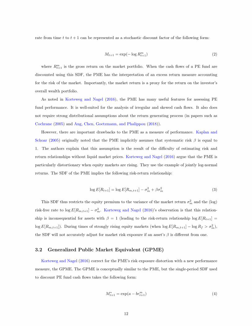
rate from time t to t+ 1 can be represented as a stochastic discount factor of the following form:

Mt+1 = exp(− logRmt+1) (2)

where Rmt+1 is the gross return on the market portfolio. When the cash flows of a PE fund are

discounted using this SDF, the PME has the interpretation of an excess return measure accounting

for the risk of the market. Importantly, the market return is a proxy for the return on the investor’s

overall wealth portfolio.

As noted in Korteweg and Nagel (2016), the PME has many useful features for assessing PE

fund performance. It is well-suited for the analysis of irregular and skewed cash flows. It also does

not require strong distributional assumptions about the return generating process (in papers such as

Cochrane (2005) and Ang, Chen, Goetzmann, and Phalippou (2018)).

However, there are important drawbacks to the PME as a measure of performance. Kaplan and

Schoar (2005) originally noted that the PME implicitly assumes that systematic risk β is equal to

1. The authors explain that this assumption is the result of the difficulty of estimating risk and

return relationships without liquid market prices. Korteweg and Nagel (2016) argue that the PME is

particularly distortionary when equity markets are rising. They use the example of jointly log-normal

returns. The SDF of the PME implies the following risk-return relationship:

logE[Rt+1] = logE[Rm,t+1]− σ2m + βσ2

m (3)

This SDF thus restricts the equity premium to the variance of the market return σ2m and the (log)

risk-free rate to logE[Rm,t+1] − σ2m. Korteweg and Nagel (2016)’s observation is that this relation-

ship is inconsequential for assets with β = 1 (leading to the risk-return relationship logE[Rt+1] =

logE[Rm,t+1]). During times of strongly rising equity markets (when logE[Rm,t+1] − logRf > σ2m),

the SDF will not accurately adjust for market risk exposure if an asset’s β is different from one.

3.2 Generalized Public Market Equivalent (GPME)

Korteweg and Nagel (2016) correct for the PME’s risk exposure distortion with a new performance

measure, the GPME. The GPME is conceptually similar to the PME, but the single-period SDF used

to discount PE fund cash flows takes the following form:

M∗t+1 = exp(a− brmt+1) (4)

12

Under this flexible SDF, the PME is a special case when a = 0 and b = 1. The authors then

compound the single-period SDF in order to find the multi-period SDF that can price cash flows over

varying time horizons. For each cash flow j, the multi-period SDF is calculated from the first cash

flow t to the payoff horizon of cash flow j, represented as h(j).

Mh(j)t+h(j) = Π

h(j)i=1M(t+ i) = exp(ah(j)− bfh(j)t+h(j)) (5)

In the log-normality example from the previous subsection, this SDF implies the log-linear β pricing

relationship in Equation 6 that appropriately accounts for market risk exposure (when a and b are

estimated to reflect the market return and risk-free rate). We describe the estimation procedure for

parameters a and b in Section 4.1 and Appendix A.

logE[Rt+1] = rf + β(logE[Rm,t+1]− rf ) (6)

The GPME takes a benchmarking perspective, asking how an investment adds value to an investor’s

portfolio that would not be attainable from other factors. Instead of using a ratio as in the classic

PME formulation in Kaplan and Schoar (2005), the GPME in Korteweg and Nagel (2016) is defined as

the sum of discounted distributions minus the sum of discounted contributions, using the multi-period

discount rate:

GPMEi =

J∑j=1

Mh(j)t+h(j)Distributionsi,t+h(j) −

J∑j=1

Mh(j)t+h(j)Callsi,t+h(j) (7)

Each cash flow is discounted to time t, including the initial investment. Moreover, each cash flow

is normalized by the size of the fund. Because of this, the GPME can be described as the NPV of $1

invested in the fund. Under the null hypothesis of no abnormal performance, E[GPMEi] = 0.

The GPME has its own limitations. Gredil, Sorensen, and Waller (2019) show that an NPV-based

estimator of fund performance may suffer more bias for samples with longer fund life, something

we confirm in Appendix C.3. Nonetheless, we show in Appendix B.3 that our results are not due to

different fund lives for our benchmark funds. We also show in Appendix C.1 and C.2 that our approach

is robust to concerns about finite sample performance and number of cash flows.

3.3 Prediction Development

In this section, we explain how we can characterize risk and performance properties of different

asset classes using the properties of PME and GPME. We start with predictions regarding market

13

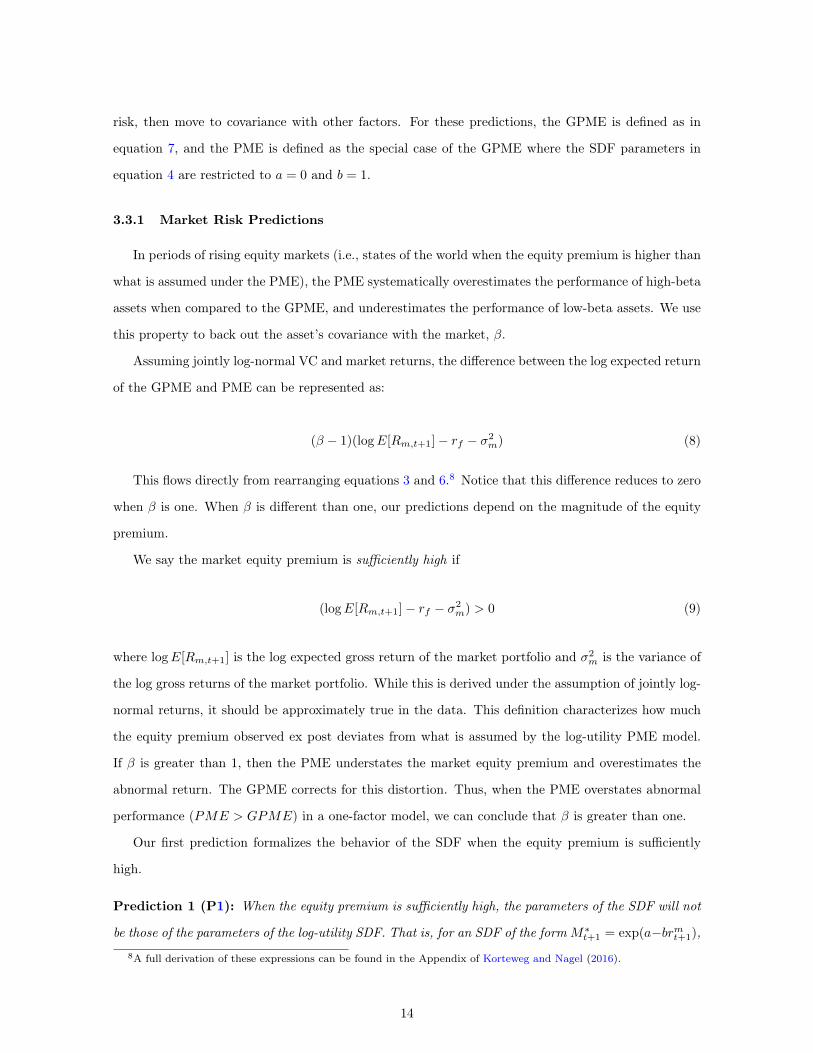
risk, then move to covariance with other factors. For these predictions, the GPME is defined as in

equation 7, and the PME is defined as the special case of the GPME where the SDF parameters in

equation 4 are restricted to a = 0 and b = 1.

3.3.1 Market Risk Predictions

In periods of rising equity markets (i.e., states of the world when the equity premium is higher than

what is assumed under the PME), the PME systematically overestimates the performance of high-beta

assets when compared to the GPME, and underestimates the performance of low-beta assets. We use

this property to back out the asset’s covariance with the market, β.

Assuming jointly log-normal VC and market returns, the difference between the log expected return

of the GPME and PME can be represented as:

(β − 1)(logE[Rm,t+1]− rf − σ2m) (8)

This flows directly from rearranging equations 3 and 6.8 Notice that this difference reduces to zero

when β is one. When β is different than one, our predictions depend on the magnitude of the equity

premium.

We say the market equity premium is sufficiently high if

(logE[Rm,t+1]− rf − σ2m) > 0 (9)

where logE[Rm,t+1] is the log expected gross return of the market portfolio and σ2m is the variance of

the log gross returns of the market portfolio. While this is derived under the assumption of jointly log-

normal returns, it should be approximately true in the data. This definition characterizes how much

the equity premium observed ex post deviates from what is assumed by the log-utility PME model.

If β is greater than 1, then the PME understates the market equity premium and overestimates the

abnormal return. The GPME corrects for this distortion. Thus, when the PME overstates abnormal

performance (PME > GPME) in a one-factor model, we can conclude that β is greater than one.

Our first prediction formalizes the behavior of the SDF when the equity premium is sufficiently

high.

Prediction 1 (P1): When the equity premium is sufficiently high, the parameters of the SDF will not

be those of the parameters of the log-utility SDF. That is, for an SDF of the formM∗t+1 = exp(a−brmt+1),

8A full derivation of these expressions can be found in the Appendix of Korteweg and Nagel (2016).

14

a 6= 0 and b 6= 1.

When Prediction 1 is true, then the distortions of the PME will be relevant for assets with a β

different from one. From Equation 8, we derive the following prediction.

Prediction 2 (P2): When the market equity premium is sufficiently high, PME overstates abnormal

performance for high-beta (β>1) assets and understates abnormal performance for low-beta (β<1)

assets. If PME = GPME, then β = 1.

We use our predictions to compare the β of impact to the β of a set of benchmark funds. From

Equation 8, within the same time period, the distortion of PME relative to GPME depends on the

magnitude of β. Defining the PME wedge as PME −GPME, we make the following prediction.

Prediction 3 (P3): When the market equity premium is sufficiently high, and all else equal, the

relative magnitude of the PME wedge reflects the relative magnitude of the asset’s beta. If (PME −

GPME)Benchmark > (PME −GPME)Imp, then βBenchmark > βImp.

We also use artificially levered cash flows to give more accurate bounds on β. This exercise was

first developed in Korteweg and Nagel (2016). We simulate increasing β by increasing a leverage factor

k applied to fund cash flows and then estimating the PME and GPME of the levered cash flows using

the original SDFs. The levered cash flows are calculated as:

Li,t+h(j) = Ci,t+h(j) + k(Ci,t+h(j) − Cif,t+h(j)) (10)

where Ci,t+h(j) are the cash flows from the original fund and Cif,t+h(j) are the cash flows from the

risk-free rate replicating portfolio which matches the capital call schedule of the original fund while

investing in the risk-free asset. Funds are indexed by i, t is time, j denotes cash flow time, h(j) denotes

time horizon, and k is a leverage factor. We assume k ≥ −1, i.e. no net short-selling of the original

fund cash flows.

When the asset has a positive β with no leverage, imposing more leverage to the cash flows will

inflate the β of levered cash flows. Reversely, if the β of the asset is negative with zero leverage,

levering up will decrease β. Thus if the unlevered β of the cash flows is positive, then the PME wedge

increases as the artificial leverage factor increases. This reflects the fact that the PME becomes a

worse measure of performance as β moves away from one.

Prediction 4 (P4): When the market equity premium is sufficiently high, the PME wedge increases

with k if βunlevered > 0. The wedge decreases with k if βunlevered < 0.

15

Building on Prediction 2, the PME wedge should be positive when k is such that the levered β is

greater than one, and negative when k is such that the levered β is less than one.

Prediction 5 (P5): When the market equity premium is sufficiently high, the PME wedge is positive

when k is such that βk > 1, and negative when k is such that βk < 1. The wedge crosses the x axis

when k is such that βk = 1.

Combining P4 and P5, we can back out approximate asset β by looking at the plot of the PME

wedge against the leverage factor k. If the wedge is decreasing, β < 0; if the wedge is increasing but

less than 0 at k = 0, then 0 < β < 1; and if the wedge is increasing and greater than 0 at k = 0, then

β > 1. We use these predictions to determine whether impact behaves like a “luxury good,” in a very

pro-cyclical way, or whether it is more of a hedging strategy as suggested by Gibson et al. (2019) and

Wang and Sargis (2020).

3.3.2 Predictions for Covariance with Other Factors

So far we have limited ourselves to a CAPM model where the return on the market portfolio

represents the return on the investor’s wealth portfolio. We may care about covariance with other

factors, for example a public sustainability factor. We can use the same intuition for different public

market indexes that may reasonably capture alternative assets that represent the impact investor’s

wealth portfolio.

We start by generalizing Equation 8 to any public-market factor X.

(β − 1)(logE[RX,t+1]− rf − σ2X) (11)

Our predictions now depend on the magnitude of the equity premium for X. The equity premium

of public-market factor X is sufficiently high if

(logE[RX,t+1]− rf − σ2X) > 0 (12)

The equity premium is low (not sufficiently high) if

(logE[RX,t+1]− rf − σ2X) < 0 (13)

When the equity premium is low, the PME overstates the public equity premium and underestimates

the abnormal return when βX > 1. In that case, when PMEX > GPMEX , we can conclude that

16

βX < 1.

Prediction 6 (P6): If the equity premium is sufficiently high for a public market factor X, then a

positive PME wedge implies a βX > 1 for that factor.

If the equity premium is low for a public market factor X, then a negative wedge implies a βX > 1

for that factor.

Similarly, we can apply the logic of P4 and P5 and use artificial leveraging in these one-factor

models to back out the covariance structure of impact investing returns relative to public market

factor X.

Prediction 7 (P7): If the equity premium is sufficiently high for a public market factor X, then a

positive relationship between the PME wedge and the amount of artificial leverage applied to cash flows

indicates a βX > 0 for that factor.

If the equity premium is low for a public market factor X, then a negative relationship between the

PME wedge and the amount of artificial leverage applied to cash flows indicates a βX > 0.

Finally, we can examine the risk profile of impact investing cash flows more generally using mul-

tifactor models. In these exercises, we examine what publicly traded factors span impact investing

returns. To undertake this analysis, we test whether impact and benchmark cash flows have abnormal

performance when discounted with SDFs that account for different risk factors.

Prediction 8 (P8): If impact investing returns are spanned by public market factors, then the GPME

with respect to these factors is zero when cash flows are discounted with a multifactor SDF.

A significant non-zero GPME with a multifactor SDF indicates that impact investing cannot be

replicated with these public market factors.

4 Impact Investing Funds and Market Risk

In this section, we test how constrained impact investing strategies perform relative to public and

private markets. To do so, we approximate the return on the impact investor’s wealth portfolio with

the return on the market and examine implications for risk and risk-adjusted performance relative to

the market. We first examine each strategy’s performance through PME and GPME, then compare

strategies using long-short portfolios. Our third subsection focuses on the market risk exposure, or

beta, of each strategy.

17

4.1 PME and GPME Estimation with Market Factor

We use two SDFs to price impact and PE cash flows: the GPME is abnormal performance when

the SDF MGPMEt+1 = exp(a− b log(Rm,t+1)) is used to price cash flows; the PME restricts this SDF to

a special case where a = 0 and b = 1.

We begin by estimating the parameters for MGPMEt+1 . We follow Korteweg and Nagel (2016) and

create public market replicating portfolios of the risk-free rate and the gross market return, for each

impact, VC, and matched fund in our sample. The purpose of these public market replicating portfolios

is to create a cash flow series for an investor that invests in and receives distributions from public assets

at roughly the same time intervals as the fund cash flow series we are interested in pricing. We then use

GMM to find the parameters of the stochastic discount factor such that the expected sum of discounted

cash flows across all replicating portfolios is equal to zero. In order to create a consistent measure of

performance, we price public market portfolios that replicate impact, VC, and matched funds, and use

the one set of parameters throughout our analysis. More details on the estimation method and the

relevant assumptions can be found in Appendix A.

The results of our estimation of SDF parameters are in Table 2. In the first column, the PME

implicitly assumes that the coefficient associated with the risk-free rate (a) is 0 and the slope coefficient

on the market return (b1) is 1. Our estimates in the second column demonstrate that the ex-post SDF is

very different from the PME assumptions. Using the procedure described above to estimate the realized

SDF, we find the slope coefficient on the log market return is 3.913 and the coefficient associated with

the risk-free rate is 0.195. These estimates are consistent with relatively “hot” equity markets and

Prediction 1.

We examine the magnitude of the market equity premium more directly by computing a sample

estimate for our sample period:

log Rm − rf − S2m ≈ 0.002 > 0

where log Rm is the natural logarithm of sample expected gross return of the market portfolio and

S2m is the sample variance of the log returns. This is consistent with a sufficiently high market equity

premium during our time period. The market risk of impact funds is thus a relevant concern for

understanding performance, and PME will distort performance upwards for riskier assets.

We now examine how the SDFs from Table 2 price the impact and VC fund cash flows. From

18

equation 7, fund-level GPME is given by:

GPMEi =

J∑j=1

Mh(j),GPMEt+h(j) Ci,t+h(j)

For fund i, cash flow time j, cash flow horizon h(j), and cash flows C. Fund-level PME is given as:

PMEi =

J∑j=1

Mh(j),PMEt+h(j) Ci,t+h(j)

In Table 3, we report the average performance of impact and benchmark (VC and matched) funds

under PME and under the market risk GPME SDF, using the SDF parameters from Table 2. We

report standard errors in parentheses and p-values of the J-test of whether (G)PME = 0 in brackets.9

Panel (a) presents our results for impact funds. We find a negative impact PME of −$0.20 per $1

of capital committed. The p-value is small, but this in part reflects the fact that the SDF parameters

for the PME are assumed (a = 0 and b = 1) rather than estimated. We also find that the market risk

GPME of impact funds is negative and statistically different from zero. After properly accounting for

risk, impact funds underperform the market index by $0.45 per $1. The overestimation of the PME

relative to the GPME suggests that impact has a market β greater than 1, in line with Prediction 2.

The underperformance of impact investing relative to public markets is consistent with the general

underperformance of constrained strategies.

However, impact’s underperformance relative to the market appears to reflect the broader under-

performance of VC over the same time period. In panel (b), we show the VC PME is also negative,

if slightly less so than the impact PME: an abnormal loss of $0.13 per $1 of capital committed. The

VC GPME is similar to the impact GPME, at a risk-adjusted loss of $0.44 per $1 of capital com-

mitted. We can reject zero pricing errors. As with impact, the PME overestimates the performance

of VC. These results are consistent with a β of VC larger than 1 (Prediction 2), as has been found

in previous literature (see e.g. Boyer et al. (2018),Cochrane (2005)). Appropriately accounting for

risk exposure suggests that an investor would fare about equally poorly adding impact or VC to her

portfolio. The similar performance of these two private market strategies suggests that private markets

are imperfectly integrated, as in Cole et al. (2020).

We report the results for the matched benchmark funds in panel (c). We find a less negative PME

of −$0.03 per $1 capital committed for this group, and a GPME of −$0.31. We cannot reject zero

pricing errors with either measure. The PME-GPME wedge is larger than impact, but smaller than9For our J-test, we adjust the spectral density matrix for correlation between pricing errors as well as estimation error

when applicable (see Appendix A for more details).

19

VC, suggesting that matched funds have a market risk exposure in between that of impact funds and

that of VC funds. A public market equity investor would seem to do slightly better investing in the

matched group of funds than in impact. We evaluate this claim next.

4.2 Long-Short Portfolios

We directly test the performance of impact relative to the two PE benchmarks by creating portfolios

of cash flows that go long $1 in each benchmark and short $1 in impact funds. This is not a replicable

strategy, but is meant to test relative differences in performance between the benchmarks and impact.

We do this in two ways. First, we look at equal-weighted long-short portfolios as statistical tests of

the PME and GPME differences in Table 3. Second, we consider value-weighted long-short portfolios

to give us a better picture of the performance of the asset class as a whole.

4.2.1 Equal-Weighted Long-Short Portfolios

To conduct statistical tests of performance differences in Table 3 between impact and benchmark

funds, we use the SDF estimates from Table 2 to price 14 equal-weighted cash flow portfolios that go

“long” benchmark funds and “short” impact funds. We create these portfolios by taking equal-weighted

averages of all benchmark or impact funds with the same vintage year. Each of the 14 portfolios then

corresponds to a vintage year in the impact sample. We normalize each of the long-short portfolios’

cash flows so that the portfolios reflect the relative number of funds in each vintage. Another way to

think of this exercise conceptually is as the return on a strategy that invests $1 in a randomly selected

benchmark fund and sells $1 in a randomly selected impact fund.

We present estimates of the PME and GPME for the 14 equal-weighted portfolios in Table 4. Panel

(a) presents results using VC funds on the long side, and Panel (b) presents results using matched

funds on the long side (both go short impact funds). The first column in both panels contains the PME

estimates that assume the strategy has β = 0, effectively discounting the long-short cash flows by the

risk-free rate. The second column contains the GPME estimates. Both PME and GPME estimates of

these strategies are positive, but we can only reject zero pricing errors in the case of the PME, where

we restrict the SDF to a = 0 and b = 1. When we adjust for market risk exposure with the GPME,

we can no longer reject zero pricing errors; in other words, we can no longer reject comparable market

risk-adjusted performance for impact funds relative to benchmark funds.

20

4.2.2 Value-Weighted Long-Short Portfolios

We also price value-weighted long-short portfolios in order to better measure relative performance

differences between a marginal dollar invested in nonimpact and impact strategies. Conceptually, we

invest $1 in the basket of benchmark funds available in our time period, and sell $1 in the basket of

impact funds available during the same time.

We do this exercise for two reasons. First, most performance benchmarks across asset classes

are market-value weighted. Second, equal weighted portfolios may be more likely to misrepresent

performance in the case of impact investing. This is because a marginal dollar invested in impact is

more likely to be invested in larger funds, but the impact market as a whole is comprised of very small

funds. As a result, equal-weighted portfolios will overweight smaller funds relative to their proportion

of capital in the asset class. While equal-weighting measures the return on a randomly selected fund,

value-weighting measures the return on a randomly invested dollar.

We approximate this conceptual exercise by creating fund size-weighted portfolios of fund cash flows

for each vintage year in the sample. These portfolios are constructed as a short portfolio of impact

funds’ size-weighted cash flows subtracted from a long portfolio of benchmark funds’ size-weighted

cash flows. The result is 14 weighted long-short portfolios of cash flows, one for each vintage year in

the impact sample. Because the distribution of vintages in the impact fund sample differs from the

overall distribution of PE fund vintages, we normalize vintage long-short portfolio cash flows such that

the cash flows in each vintage reflects that vintage’s size relative to other vintages.

Table 5 presents the PME and GPME estimates of our value-weighted portfolios, using SDF es-

timates from Table 2. The PME and GPME of this value-weighted long-short strategy reflect the

performance of benchmark funds relative to impact funds for an investor with a stake in the basket

of impact funds during our sample period. Again, Panel (a) presents results using VC funds on the

long side, and Panel (b) presents results using matched funds on the long side. Value-weighting yields

smaller estimates than equal-weighting, reflecting the influence of smaller funds and vintages. When

smaller funds and vintages are given less weight, the performance of benchmark funds relative to im-

pact funds worsens. PME estimates remain positive but smaller than those in Table 4, and GPME

estimates become negative.

On a value-weighted basis, the risk-adjusted returns of going long VC and shorting impact are

negative, −$0.15 per $1 of committed capital, and we can reject zero pricing errors. We cannot

reject zero pricing errors for PME estimates or for the GPME estimate of the portfolio that goes long

in matched funds and short in impact funds. We conclude that impact performs better as a class

21

than VC in our sample period, and neither better nor worse than the sample of matched funds. While

constrained strategies do worse on both an absolute and risk-adjusted basis relative to an unconstrained

strategy (investing in a public market index), our results suggest that impact investors can do as well

as other private market investors. This is potentially due to impact investing extracting value from

private market frictions, such as information barriers.

Whether value- or equal-weighted, we find positive PMEs and a postive wedge between the PME

and GPME estimates of the long-short strategies. We can conclude that the β of these strategies are

not zero because the GPME and PME estimates are not the same. In line with Prediction 3, our

results indicate that βBenchmark > βImp. We examine the relative β of both strategies in more detail

in the next section.

4.3 Backing Out Market Risk Exposure Using Artificial Leverage

The relatively small PME wedge of impact relatively to the other private market strategies suggests

that impact funds have a low β with public markets. In this section, we use artificial leverage to bound

the β of impact relative to our two benchmarks, and thus inform the debate about the risk of sustainable

and green assets. We use the SDF estimates in Table 2 to price levered cash flows given in equation 10.

We apply this leverage strategy first to the fund cash flows directly, then to the cash flows from our

long-short portfolio strategy.

4.3.1 PME-GPME Wedges

We plot the PME wedge for impact and both benchmarks in Figure 8. We create 95% confidence

intervals by bootstrapping the wedge estimates 1,000 times. At k = 0, there is no additional leverage

and the wedge is the difference between the PME and GPME estimates as in Section 4.1. As we

increase k to a leverage factor of 1 and 2, we artificially increase the β of the cash flows. Thus,

for any asset with a positive β, we expect an increasing wedge with the addition of more leverage

(Prediction 4). If an asset is already a high-beta asset at k = 0, this additional leverage should lead

to an increasing wedge as the PME becomes a more distortionary measure of performance. If an asset

has a β = 1, then the GPME and PME should coincide at k = 0 and we would expect to see a positive

slope with the addition of more leverage, crossing the x axis at k = 0.

We can also apply negative leverage to the cash flows, replicating a decrease in β. Given a high-beta

asset, we can determine how much de-leveraging is necessary to achieve a β = 1 by examining at what

value of k the wedge is equal to zero. As k nears −1, the wedge should become negative as levered β

falls below one and the PME begins to understate performance.

22

The line for VC funds is consistent with Predictions 4 and 5: as the leverage factor and thus β

increase, the PME wedge increases as well, as we would expect for a high-beta asset. The wedge is also

close to 0 around leverage factor -0.5. These two findings, along with those from the previous section,

suggest a VC β of approximately 1/0.5 = 2 > 1.

In contrast, the wedge for impact appears relatively flatter across leverage factors, only slightly

increasing in k. A constant wedge would imply a β close to zero, as additional leverage does not affect

the wedge magnitude. However, we can reject a zero wedge at k = 0 with 95% confidence, suggesting

that β must be at least one. The relatively flat slope of the wedge line suggests that β is not much

higher than one. We cannot infer more specifics about the absolute level of impact β from Figure 8,

but we can rule out that the sensitivity is as large as VC. This reinforces our conclusion from Table ??

that βV C > βImp.

The matched fund wedge is flatter than the VC line, but steeper than impact. At higher factors of

leverage, the separation across the three strategies becomes clearer, with VC most sensitive to market

risk, impact least, and the matched benchmark in between. The higher sensitivity of the matched

benchmark to leverage factors suggests that impact’s lower β is not entirely explained by size, asset

class, or vintage. We do not find impact is countercyclical in absolute, but adding impact to a VC

portfolio does reduce overall market risk exposure.

4.3.2 Long Short Portfolio Wedges

To supplement this analysis, we also apply artificial leverage to the value-weighted long-short cash

flow portfolios from Section 4.2. Applying artificial leverage to the net cash flows is another way to test

both whether the β of the benchmarks and impact are different and whether the β of the benchmarks

are greater than the β of impact. If a benchmark and impact β are the same, then the β of that

long-short portfolio should be zero, and the PME wedge should stay constant as we increase k.

We can formalize this intuition in the context of the jointly log-normal model used at the outset

of Section 3 in Equation 8. From equation 11, the wedge for benchmark B under jointly log-normal

returns is:

(βB − 1)(logE[Rm,t+1]− rf − σ2m)

The wedge for impact is then:

(βImp − 1)(logE[Rm,t+1]− rf − σ2m)

23

This implies that the wedge of the net cash flows is:

(PMEB −PMEImp)− (GPMEB −GPMEImp) = (PMEB −GPMEB)− (PMEImp −GPMEImp)

Which can then be written as

(βB − 1)(logE[Rm,t+1 − rf − σ2m)− (βImp − 1)(logE[Rm,t+1]− rf − σ2

m)

Given that the equity premium is the same in both samples, this expression reduces to:

(βB − βImp)(logE[Rm,t+1]− rf − σ2m) (14)

Given a large market equity premium (relative to σ2m), a positive wedge is indicative of βB−βImp > 0. A

negative wedge indicates that βB−βImp < 0. If the equity premium was small (i.e., logE[Rm,t+1]−rf <

σ2m), then the opposite predictions would hold.

What we observe in Figure 9 is a wedge that is increasing in artificial leverage k for both benchmarks.

The positive slope of both lines indicates that the β of the net cash flows is positive: as k increases,

the GPME becomes more negative and the wedge increases. This is further evidence that the β of

both benchmarks is greater than the β of impact, although we note that our confidence intervals are

too large to statistically reject a zero wedge at any value of the leverage factor. We see these results as

further suggestive evidence that impact investing provides market hedging services beyond its features

(size, asset class) as a private equity class.

5 Impact Investing Funds and Other Factors

What other financial risks are inherent in an impact investing strategy? Section 4 characterizes the

market β of impact funds, i.e., the covariance of these cash flows with the market. In this section, we

use the same tools to characterize the covariance of impact fund cash flows with other factors. We first

examine whether private sustainable investing is different from public sustainable investing strategies.

Then we test whether additional risk factors span impact investing cash flows.

5.1 Abnormal Performance and Risk Exposure to Other Factors

We can approximate the covariance of impact fund cash flows with any factor by replicating the

analysis in Section 4, using a one-factor SDF with the alternative factor of interest in place of the

24

Market Risk SDF. Predictions 6 and 7 highlight that the interpretation of the analysis depends on the

magnitude of the public market premium with that factor. If the market premium for the factor of

interest is sufficiently high, then predictions are the same as for the market factor. However, if the

market premium is low, our predictions flip.

We investigate impact and benchmark funds’ risk exposure to a sustainability index factor. We

start by examining the magnitude of the equity premium on the sustainability index by computing its

sample estimate:

log RSI − rf − S2SI ≈ −0.002 < 0

where log RSI is the natural logarithm of sample expected gross return of the sustainability index and

S2SI is the sample variance of the log returns. This corresponds to the scenario in which the equity

premium is low.We are in the second case of Prediction 6: a negative PMESI wedge would imply a

βSI > 1 with the sustainability index.

Table 6 reports the one-factor SDF estimate and Table 7 gives the PME and GPME estimates

using the sustainability index as the public market return of interest. Our estimates show that the

ex-post SDF using sustainability as the benchmark is also very different from the SDF with log-

utility assumptions. We find a slope coefficient on log sustainability returns of 2.49 and an intercept

coefficient of 0.06. The PME and GPME estimates are different between impact, VC, and matched

funds. With risk adjustment relative to the sustainability index, VC funds gain $0.15 and matched

funds gain $0.28 per $1 capital committed, while impact funds lose $0.16 per $1 capital committed.

The overperformance of benchmark funds relative to the sustainability index is consistent with a

concessionary return for sustainable strategies in public markets. The PME overestimates impact

fund performance and underestimates VC and matched fund performance relative to the GPMESI .

However, given the wide error bands on all of the GPME estimates, we cannot draw conclusions on

sustainability β by looking at the “wedge” with zero leverage.

In Figure 10, we show what happens to the wedge for different levels of artificial leverage. Since

the sustainability premium is relatively small, we are in the second case of Prediction 7: an increasing

wedge, as we see for VC and impact funds, implies negative covariance with the sustainability index.

A decreasing wedge, as we see for matched funds, implies positive covariance with the sustainability

index. The bounds on these estimates are large and the results should be taken with caution, but

they highlight that sustainability in private markets, for example via impact investing, is distinct from

sustainability in public markets.

25

5.2 PME and GPME Estimation with Two Factors

The one-factor GPME model can be extended to incorporate multiple factors. The SDF in this

case is

MGPMEt+1 = exp(a− b′ log(Ft+1))

where f is the number of public market factors, b is an f × 1 vector of factor loadings, and log(Ft+1)

is f × 1 vector of public market factor returns at time t+ 1.

We use the simplest multi-factor GPME with f = 2 to test whether impact, VC, and matched

fund returns can be spanned by additional risk factors. We augment the Market Risk SDF with a

sustainability factor or the small-growth portfolio from Fama and French (1993). The results are in

Table 8. As in Table 3, Panel (a) provides estimates for impact funds, Panel (b) for VC funds, and

Panel (c) for matched funds. In the first column, we repeat the GPME estimates from the one-factor

market risk model as a reference. The last two columns correspond to two-factor SDFs with the

market and small-growth portfolio (second column) or with the market and sustainability index (third

column).

Our first observation is that, consistent with Korteweg and Nagel (2016), adding the small-growth

factor has little effect on the GPME for VC funds. Replacing the small-growth factor with the sustain-

ability index produces similar results. For VC funds, we find a negative GPME of −$0.42 to −$0.44

per $1 of capital committed in all three specifications.

We run the same three models on our impact funds. Similar to Market Risk SDF, we get an

abnormal performance of −$0.42 per $1 invested after adding the small-growth factor. Adding the

sustainability index yields a higher estimate of −$0.33. We cannot reject zero pricing errors in this

model, which implies that these two factors span impact returns. However, the standard error for this

estimate is large. An interval of a single standard error would encompass the GPME estimates in the

other two specifications.

For matched funds, we find an abnormal performance of −$0.28 per $1 committed after adding the

small-growth factor, which is similar to −$0.31 with the Market Risk SDF. Adding the sustainability

index to the market factor also does not change the estimate much, at −$0.30 per $1 committed.

For VC funds, we can reject zero pricing errors in all models, and find a significant abnormal loss

both economically and statistically. We can reject zero pricing errors for impact funds in the first

two models, and find negative performance on par with VC’s negative performance. We cannot reject

zero pricing errors for impact funds when we add the sustainability index as a factor, though the

point estimate remains significantly negative from an economic standpoint. Matched funds appear to

26

perform somewhat better than VC or impact funds, and we cannot reject zero pricing errors in any

of the specifications. Whatever additional factor we add, matched funds perform better than impact

and VC funds after appropriate risk adjustments, consistent with Section 4.

6 Conclusion

In this paper, we provide a characterization of the risk profile and risk-adjusted performance of

impact investing. To do this, we develop a new approach to derive risk properties of private market asset

classes, building on insights from Korteweg and Nagel (2016). While we apply it to impact investing

in this paper, our approach can easily be extended to examining other private market strategies in

the future. We use this to show, for example, that the market beta of impact funds is statistically

significantly lower than the market beta of VC funds. When accounting for market risk exposure,

impact funds underperform the market but do not perform worse than comparable private market

strategies.

Our findings shed light on theories of the market as well as the nature of green assets. Our

finding that impact underperforms both the S&P 500 and a public sustainability index is consistent

with impact investing as a constrained strategy that necessarily leads to lower returns. We find a

similar effect for VC and matched benchmark funds, suggesting that private markets violate perfect

and complete market assumptions. Our finding that impact outperforms VC funds in a value-weighted

long-short portfolio is consistent with market frictions in private markets overall. Impact investors may

be constrained, but seem to be able to capture value that general VC investors miss. This could be

due to information barriers, investor biases, or distortions to competition in both capital and product

markets.

Risk is an important element in this story. Our finding that the beta of impact is lower than the

beta of benchmarks, and in particular VC, is consistent with a counter-cyclical interpretation of impact

strategies. Although absolute measures of performance are lower during periods of hot equity markets,

impact investing acts as a relative hedge against downside risk.

27

References

Andersson, M., P. Bolton, and F. Samama (2016). Hedging climate risk. Financial Analysts Jour-

nal 72 (3), 13–32.

Ang, A., B. Chen, W. N. Goetzmann, and L. Phalippou (2018). Estimating Private Equity Returns

from Limited Partner Cash Flows. Journal of Finance 73 (4), 1751–1783.

Bansal, R., D. A. Wu, and A. Yaron (2018). Is socially responsible investing a luxury good? Available

at SSRN 3259209 .

Barber, B. M., A. Morse, and A. Yasuda (2021). Impact investing. Journal of Financial Eco-

nomics 139 (1), 162 – 185.

Boyer, B., T. D. Nadauld, K. P. Vorkink, and M. S. Weisbach (2018). Private equity indices based on

secondary market transactions. Technical report, National Bureau of Economic Research.

Brest, P., R. J. Gilson, and M. A. Wolfson (2018). Essay: How investors can (and can’t) create social

value. J. Corp. L. 44, 205.

Brown, G. W., O. R. Gredil, and S. N. Kaplan (2019). Do private equity funds manipulate reported

returns? Journal of Financial Economics 132 (2), 267–297.

Brown, G. W., R. S. Harris, T. Jenkinson, S. N. Kaplan, and D. T. Robinson (2015). What do different

commercial data sets tell us about private equity performance? Available at SSRN 2706556 .

Burton, M. D., S. A. Cole, A. Dev, C. Jarymowycz, L. Jeng, J. Lerner, F. Mashwama, C. Xu, and

R. Zochowski (2021). The project on impact investments’ impact investment database. Harvard

Business School Entrepreneurial Management Working Paper (20-117), 20–117.

Chowdhry, B., S. W. Davies, and B. Waters (2019). Investing for impact. The Review of Financial

Studies 32 (3), 864–904.

Cochrane, J. H. (2005). The risk and return of venture capital. Journal of Financial Economics 75 (1),

3–52.

Cole, S., M. Melecky, F. Mölders, and T. Reed (2020). Long-run Returns to Impact Investing in

Emerging Market and Developing Economies.

Engle, R. F., S. Giglio, B. Kelly, H. Lee, and J. Stroebel (2020). Hedging climate change news. Review

of Financial Studies 33 (3), 1184–1216.

28

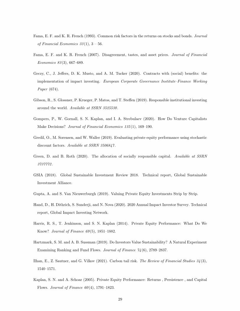
Fama, E. F. and K. R. French (1993). Common risk factors in the returns on stocks and bonds. Journal

of Financial Economics 33 (1), 3 – 56.

Fama, E. F. and K. R. French (2007). Disagreement, tastes, and asset prices. Journal of Financial

Economics 83 (3), 667–689.

Geczy, C., J. Jeffers, D. K. Musto, and A. M. Tucker (2020). Contracts with (social) benefits: the

implementation of impact investing. European Corporate Governance Institute–Finance Working

Paper (674).

Gibson, R., S. Glossner, P. Krueger, P. Matos, and T. Steffen (2019). Responsible institutional investing

around the world. Available at SSRN 3525530 .

Gompers, P., W. Gornall, S. N. Kaplan, and I. A. Strebulaev (2020). How Do Venture Capitalists

Make Decisions? Journal of Financial Economics 135 (1), 169–190.

Gredil, O., M. Sorensen, and W. Waller (2019). Evaluating private equity performance using stochastic

discount factors. Available at SSRN 3506847 .

Green, D. and B. Roth (2020). The allocation of socially responsible capital. Available at SSRN

3737772 .

GSIA (2018). Global Sustainable Investment Review 2018. Technical report, Global Sustainable

Investment Alliance.

Gupta, A. and S. Van Nieuwerburgh (2019). Valuing Private Equity Investments Strip by Strip.

Hand, D., H. Dithrich, S. Sunderji, and N. Nova (2020). 2020 Annual Impact Investor Survey. Technical

report, Global Impact Investing Network.

Harris, R. S., T. Jenkinson, and S. N. Kaplan (2014). Private Equity Performance: What Do We

Know? Journal of Finance 69 (5), 1851–1882.

Hartzmark, S. M. and A. B. Sussman (2019). Do Investors Value Sustainability? A Natural Experiment

Examining Ranking and Fund Flows. Journal of Finance 74 (6), 2789–2837.

Ilhan, E., Z. Sautner, and G. Vilkov (2021). Carbon tail risk. The Review of Financial Studies 34 (3),

1540–1571.

Kaplan, S. N. and A. Schoar (2005). Private Equity Performance: Returns , Persistence , and Capital

Flows. Journal of Finance 60 (4), 1791–1823.

29

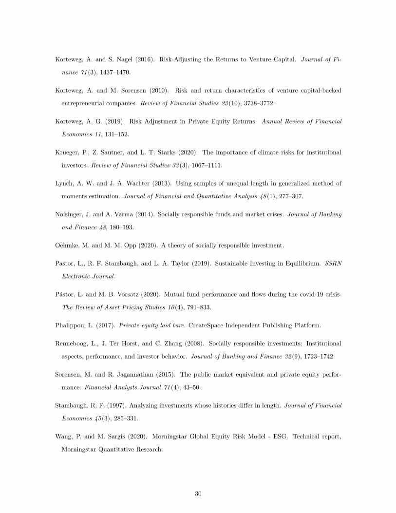
Korteweg, A. and S. Nagel (2016). Risk-Adjusting the Returns to Venture Capital. Journal of Fi-

nance 71 (3), 1437–1470.

Korteweg, A. and M. Sorensen (2010). Risk and return characteristics of venture capital-backed

entrepreneurial companies. Review of Financial Studies 23 (10), 3738–3772.

Korteweg, A. G. (2019). Risk Adjustment in Private Equity Returns. Annual Review of Financial

Economics 11, 131–152.

Krueger, P., Z. Sautner, and L. T. Starks (2020). The importance of climate risks for institutional

investors. Review of Financial Studies 33 (3), 1067–1111.

Lynch, A. W. and J. A. Wachter (2013). Using samples of unequal length in generalized method of

moments estimation. Journal of Financial and Quantitative Analysis 48 (1), 277–307.

Nofsinger, J. and A. Varma (2014). Socially responsible funds and market crises. Journal of Banking

and Finance 48, 180–193.

Oehmke, M. and M. M. Opp (2020). A theory of socially responsible investment.

Pastor, L., R. F. Stambaugh, and L. A. Taylor (2019). Sustainable Investing in Equilibrium. SSRN

Electronic Journal .

Pástor, L. and M. B. Vorsatz (2020). Mutual fund performance and flows during the covid-19 crisis.

The Review of Asset Pricing Studies 10 (4), 791–833.

Phalippou, L. (2017). Private equity laid bare. CreateSpace Independent Publishing Platform.

Renneboog, L., J. Ter Horst, and C. Zhang (2008). Socially responsible investments: Institutional

aspects, performance, and investor behavior. Journal of Banking and Finance 32 (9), 1723–1742.

Sorensen, M. and R. Jagannathan (2015). The public market equivalent and private equity perfor-

mance. Financial Analysts Journal 71 (4), 43–50.

Stambaugh, R. F. (1997). Analyzing investments whose histories differ in length. Journal of Financial

Economics 45 (3), 285–331.

Wang, P. and M. Sargis (2020). Morningstar Global Equity Risk Model - ESG. Technical report,

Morningstar Quantitative Research.

30

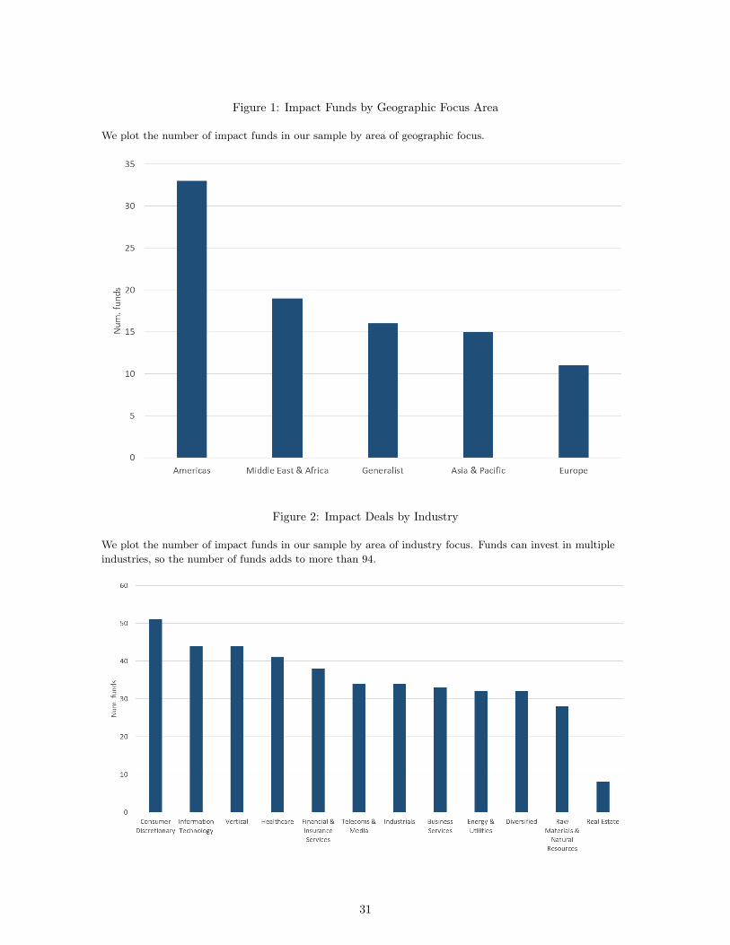
Figure 1: Impact Funds by Geographic Focus Area

We plot the number of impact funds in our sample by area of geographic focus.

Figure 2: Impact Deals by Industry

We plot the number of impact funds in our sample by area of industry focus. Funds can invest in multipleindustries, so the number of funds adds to more than 94.

31

Figure 3: Impact Funds by Asset Class

We plot the number of impact funds in our sample by asset class. VC funds are equity funds that invest withan early stage focus. Other equity funds include late stage and more generalist funds. Buyout funds areequity funds with a buyout focus that use leverage. Debt funds are private funds that originate loans toportfolio companies. Real asset funds invest in physical assets. The remainder of impact funds are generalist,that invest with a variety of styles in companies at various stages.

32

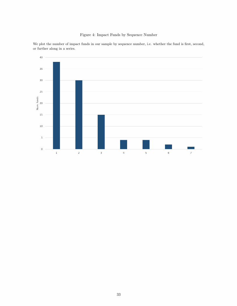
Figure 4: Impact Funds by Sequence Number

We plot the number of impact funds in our sample by sequence number, i.e. whether the fund is first, second,or further along in a series.

33

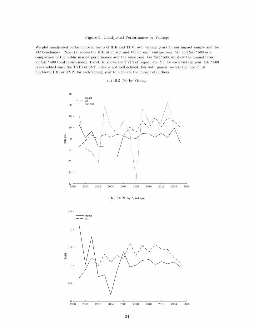
Figure 5: Unadjusted Performance by Vintage

We plot unadjusted performance in terms of IRR and TPVI over vintage years for our impact sample and theVC benchmark. Panel (a) shows the IRR of impact and VC for each vintage year. We add S&P 500 as acomparison of the public market performance over the same year. For S&P 500, we show the annual returnfor S&P 500 total return index. Panel (b) shows the TVPI of impact and VC for each vintage year. S&P 500is not added since the TVPI of S&P index is not well defined. For both panels, we use the median offund-level IRR or TVPI for each vintage year to alleviate the impact of outliers.

(a) IRR (%) by Vintage

1998 2000 2002 2004 2006 2008 2010 2012 2014 2016-40

-30

-20

-10

0

10

20

30

40

IRR

(%

)

ImpactVCS&P 500

(b) TVPI by Vintage

1998 2000 2002 2004 2006 2008 2010 2012 2014 20160

0.5

1

1.5

2

2.5

TV

PI

ImpactVC

34

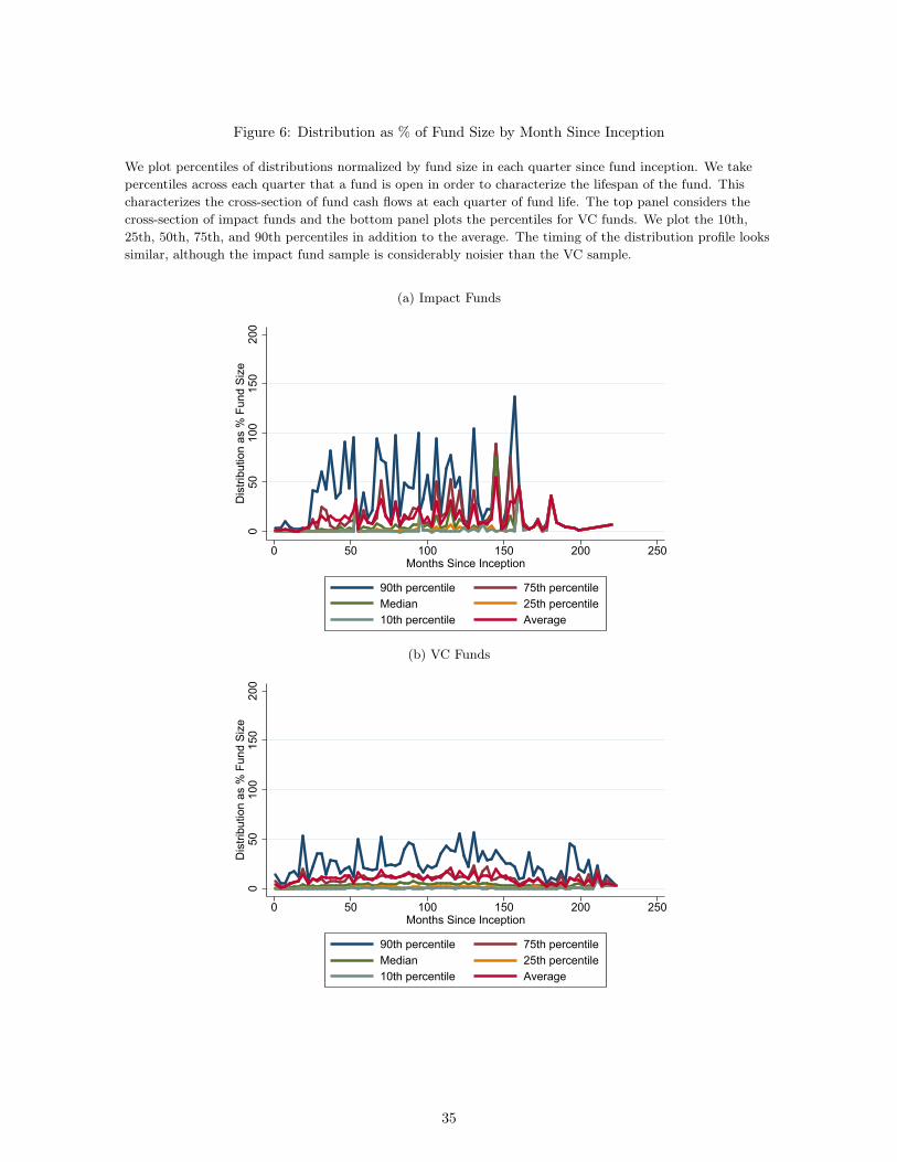
Figure 6: Distribution as % of Fund Size by Month Since Inception

We plot percentiles of distributions normalized by fund size in each quarter since fund inception. We takepercentiles across each quarter that a fund is open in order to characterize the lifespan of the fund. Thischaracterizes the cross-section of fund cash flows at each quarter of fund life. The top panel considers thecross-section of impact funds and the bottom panel plots the percentiles for VC funds. We plot the 10th,25th, 50th, 75th, and 90th percentiles in addition to the average. The timing of the distribution profile lookssimilar, although the impact fund sample is considerably noisier than the VC sample.

(a) Impact Funds

050

100

150

200

Dis

tribu

tion

as %

Fun

d Si

ze

0 50 100 150 200 250Months Since Inception

90th percentile 75th percentileMedian 25th percentile10th percentile Average

(b) VC Funds

050

100

150

200

Dis

tribu

tion

as %

Fun

d Si

ze

0 50 100 150 200 250Months Since Inception

90th percentile 75th percentileMedian 25th percentile10th percentile Average

35

Figure 7: Distribution as % of Fund Size by Year Since Inception

We plot percentiles of distributions normalized by fund size in each year since fund inception. This results ina smoothed version of Figure 6. We sum total distributions in a given year (including the final period NAV)and divide by the total committed capital of the fund. We take percentiles across each year that a fund isopen in order to characterize the cross-section of fund. As in Figure 6, the distribution profile looks similar,with an increase in distributions as a percent of fund size around years 5 to 7. The impact funds have verylarge final period NAV payouts compared to VC funds. Impact’s median distribution at each year is higherthan for VC funds.

(a) Impact Funds

050

100

150

200

Dis

tribu

tion

as %

Fun

d Si

ze

0 5 10 15 20Years Since Inception

90th percentile 75th percentileMedian 25th percentile10th percentile Average

(b) VC Funds

050

100

150

200

Dis

tribu

tion

as %

Fun

d Si

ze

0 5 10 15 20Years Since Inception

90th percentile 75th percentileMedian 25th percentile10th percentile Average

36

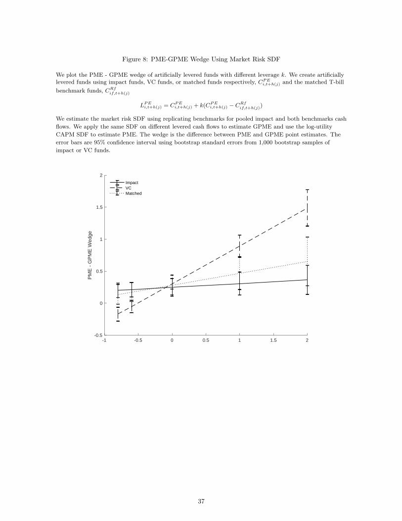
Figure 8: PME-GPME Wedge Using Market Risk SDF

We plot the PME - GPME wedge of artificially levered funds with different leverage k. We create artificiallylevered funds using impact funds, VC funds, or matched funds respectively, CPE

i,t+h(j) and the matched T-billbenchmark funds, CRf

if,t+h(j)

LPEi,t+h(j) = CPE

i,t+h(j) + k(CPEi,t+h(j) − CRf

if,t+h(j))

We estimate the market risk SDF using replicating benchmarks for pooled impact and both benchmarks cashflows. We apply the same SDF on different levered cash flows to estimate GPME and use the log-utilityCAPM SDF to estimate PME. The wedge is the difference between PME and GPME point estimates. Theerror bars are 95% confidence interval using bootstrap standard errors from 1,000 bootstrap samples ofimpact or VC funds.

-1 -0.5 0 0.5 1 1.5 2-0.5

0

0.5

1

1.5

2

PM

E -

GP

ME

Wed

ge

ImpactVCMatched

37

Figure 9: PME-GPME Wedge of Long-Short Portfolio

We create two portfolios, one that is long VC funds and short impact funds, and the other that is longmatched funds and short impact funds. Both portfolios presented here are value-weighted. We createartificially levered cash flows of each strategy similar to Figure 8. For each level of artificial leverage k, weplot the difference between the PME and GPME point estimate of the long-short portfolio. The error barsare 95% confidence interval using bootstrap standard errors from 1,000 bootstrap samples of the long-shortportfolio.

(a) Value-Weighted

-1 -0.5 0 0.5 1 1.5 2-2

-1

0

1

2

3

4

PM

E -

GP

ME

Wed

ge

Long VCLong Matched

38

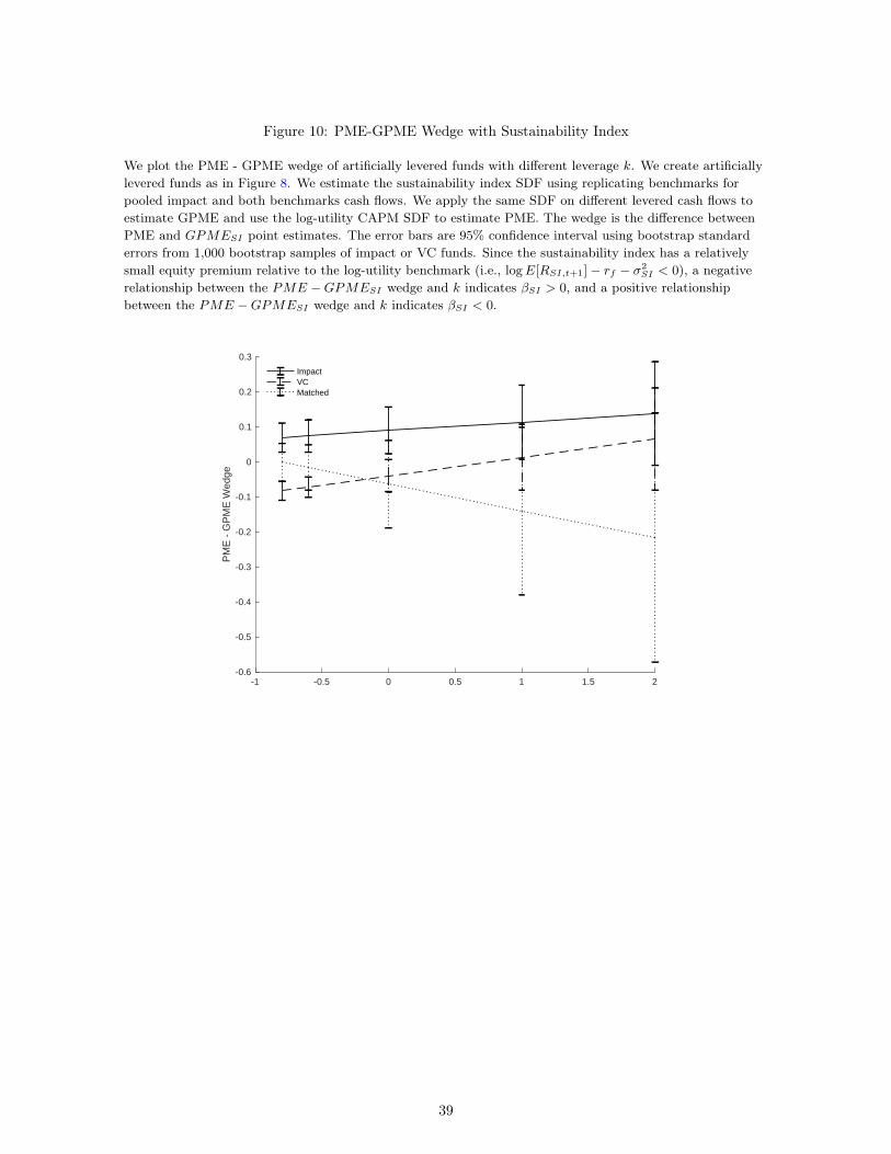
Figure 10: PME-GPME Wedge with Sustainability Index

We plot the PME - GPME wedge of artificially levered funds with different leverage k. We create artificiallylevered funds as in Figure 8. We estimate the sustainability index SDF using replicating benchmarks forpooled impact and both benchmarks cash flows. We apply the same SDF on different levered cash flows toestimate GPME and use the log-utility CAPM SDF to estimate PME. The wedge is the difference betweenPME and GPMESI point estimates. The error bars are 95% confidence interval using bootstrap standarderrors from 1,000 bootstrap samples of impact or VC funds. Since the sustainability index has a relativelysmall equity premium relative to the log-utility benchmark (i.e., logE[RSI,t+1]− rf − σ2

SI < 0), a negativerelationship between the PME −GPMESI wedge and k indicates βSI > 0, and a positive relationshipbetween the PME −GPMESI wedge and k indicates βSI < 0.

-1 -0.5 0 0.5 1 1.5 2-0.6

-0.5

-0.4

-0.3

-0.2

-0.1

0

0.1

0.2

0.3

PM

E -

GP

ME

Wed

ge

ImpactVCMatched

39

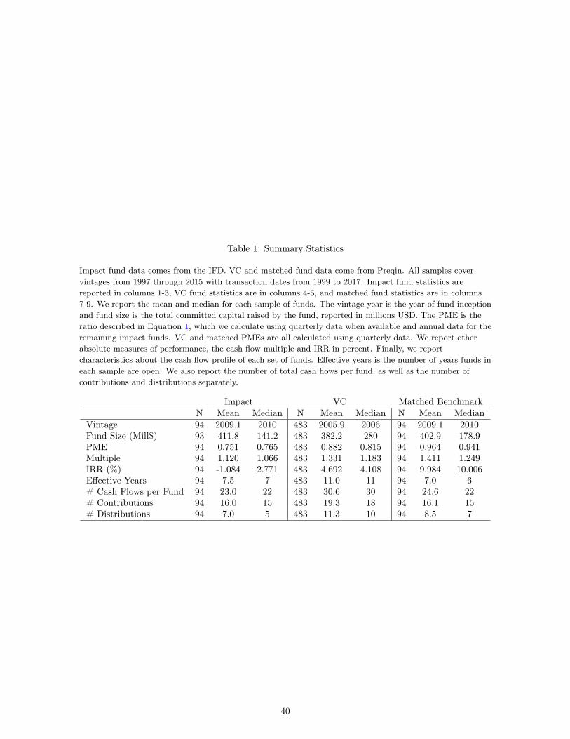
Table 1: Summary Statistics

Impact fund data comes from the IFD. VC and matched fund data come from Preqin. All samples covervintages from 1997 through 2015 with transaction dates from 1999 to 2017. Impact fund statistics arereported in columns 1-3, VC fund statistics are in columns 4-6, and matched fund statistics are in columns7-9. We report the mean and median for each sample of funds. The vintage year is the year of fund inceptionand fund size is the total committed capital raised by the fund, reported in millions USD. The PME is theratio described in Equation 1, which we calculate using quarterly data when available and annual data for theremaining impact funds. VC and matched PMEs are all calculated using quarterly data. We report otherabsolute measures of performance, the cash flow multiple and IRR in percent. Finally, we reportcharacteristics about the cash flow profile of each set of funds. Effective years is the number of years funds ineach sample are open. We also report the number of total cash flows per fund, as well as the number ofcontributions and distributions separately.

Impact VC Matched BenchmarkN Mean Median N Mean Median N Mean Median

Vintage 94 2009.1 2010 483 2005.9 2006 94 2009.1 2010Fund Size (Mill$) 93 411.8 141.2 483 382.2 280 94 402.9 178.9PME 94 0.751 0.765 483 0.882 0.815 94 0.964 0.941Multiple 94 1.120 1.066 483 1.331 1.183 94 1.411 1.249IRR (%) 94 -1.084 2.771 483 4.692 4.108 94 9.984 10.006Effective Years 94 7.5 7 483 11.0 11 94 7.0 6# Cash Flows per Fund 94 23.0 22 483 30.6 30 94 24.6 22# Contributions 94 16.0 15 483 19.3 18 94 16.1 15# Distributions 94 7.0 5 483 11.3 10 94 8.5 7

40

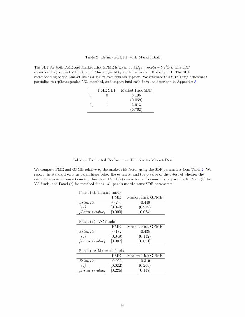
Table 2: Estimated SDF with Market Risk

The SDF for both PME and Market Risk GPME is given by M∗t+1 = exp(a− b1rMt+1). The SDF

corresponding to the PME is the SDF for a log-utility model, where a = 0 and b1 = 1. The SDFcorresponding to the Market Risk GPME relaxes this assumption. We estimate this SDF using benchmarkportfolios to replicate pooled VC, matched, and impact fund cash flows, as described in Appendix A.

PME SDF Market Risk SDFa 0 0.195

(0.069)b1 1 3.913

(0.762)

Table 3: Estimated Performance Relative to Market Risk

We compute PME and GPME relative to the market risk factor using the SDF parameters from Table 2. Wereport the standard error in parentheses below the estimate, and the p-value of the J-test of whether theestimate is zero in brackets on the third line. Panel (a) estimates performance for impact funds, Panel (b) forVC funds, and Panel (c) for matched funds. All panels use the same SDF parameters.

Panel (a): Impact fundsPME Market Risk GPME

Estimate -0.200 -0.448(sd) (0.040) (0.212)[J-stat p-value] [0.000] [0.034]

Panel (b): VC fundsPME Market Risk GPME

Estimate -0.132 -0.435(sd) (0.049) (0.132)[J-stat p-value] [0.007] [0.001]

Panel (c): Matched fundsPME Market Risk GPME

Estimate -0.026 -0.310(sd) (0.022) (0.209)[J-stat p-value] [0.226] [0.137]

41

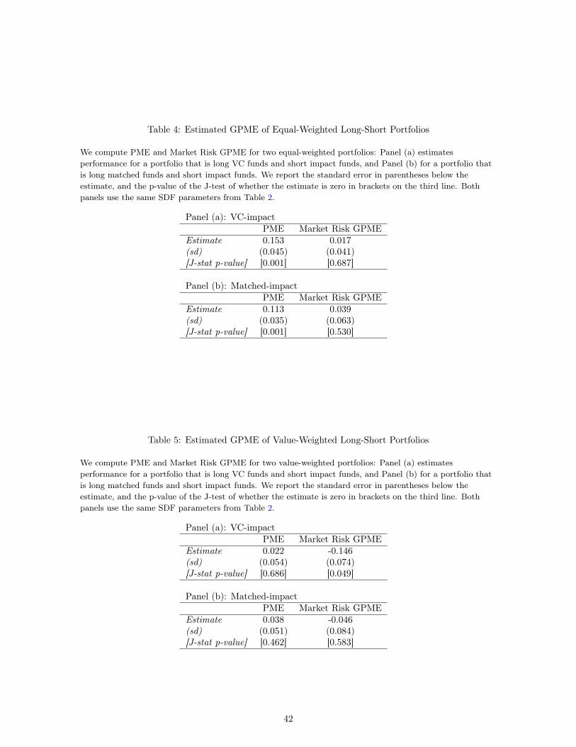
Table 4: Estimated GPME of Equal-Weighted Long-Short Portfolios

We compute PME and Market Risk GPME for two equal-weighted portfolios: Panel (a) estimatesperformance for a portfolio that is long VC funds and short impact funds, and Panel (b) for a portfolio thatis long matched funds and short impact funds. We report the standard error in parentheses below theestimate, and the p-value of the J-test of whether the estimate is zero in brackets on the third line. Bothpanels use the same SDF parameters from Table 2.

Panel (a): VC-impactPME Market Risk GPME

Estimate 0.153 0.017(sd) (0.045) (0.041)[J-stat p-value] [0.001] [0.687]

Panel (b): Matched-impactPME Market Risk GPME

Estimate 0.113 0.039(sd) (0.035) (0.063)[J-stat p-value] [0.001] [0.530]

Table 5: Estimated GPME of Value-Weighted Long-Short Portfolios

We compute PME and Market Risk GPME for two value-weighted portfolios: Panel (a) estimatesperformance for a portfolio that is long VC funds and short impact funds, and Panel (b) for a portfolio thatis long matched funds and short impact funds. We report the standard error in parentheses below theestimate, and the p-value of the J-test of whether the estimate is zero in brackets on the third line. Bothpanels use the same SDF parameters from Table 2.

Panel (a): VC-impactPME Market Risk GPME

Estimate 0.022 -0.146(sd) (0.054) (0.074)[J-stat p-value] [0.686] [0.049]

Panel (b): Matched-impactPME Market Risk GPME

Estimate 0.038 -0.046(sd) (0.051) (0.084)[J-stat p-value] [0.462] [0.583]

42

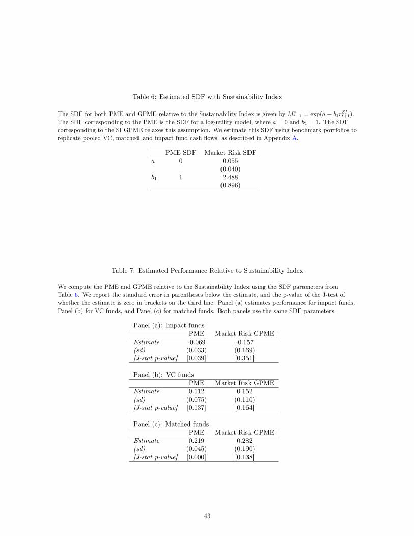
Table 6: Estimated SDF with Sustainability Index

The SDF for both PME and GPME relative to the Sustainability Index is given by M∗t+1 = exp(a− b1rSIt+1).

The SDF corresponding to the PME is the SDF for a log-utility model, where a = 0 and b1 = 1. The SDFcorresponding to the SI GPME relaxes this assumption. We estimate this SDF using benchmark portfolios toreplicate pooled VC, matched, and impact fund cash flows, as described in Appendix A.

PME SDF Market Risk SDFa 0 0.055

(0.040)b1 1 2.488

(0.896)

Table 7: Estimated Performance Relative to Sustainability Index

We compute the PME and GPME relative to the Sustainability Index using the SDF parameters fromTable 6. We report the standard error in parentheses below the estimate, and the p-value of the J-test ofwhether the estimate is zero in brackets on the third line. Panel (a) estimates performance for impact funds,Panel (b) for VC funds, and Panel (c) for matched funds. Both panels use the same SDF parameters.

Panel (a): Impact fundsPME Market Risk GPME

Estimate -0.069 -0.157(sd) (0.033) (0.169)[J-stat p-value] [0.039] [0.351]

Panel (b): VC fundsPME Market Risk GPME

Estimate 0.112 0.152(sd) (0.075) (0.110)[J-stat p-value] [0.137] [0.164]

Panel (c): Matched fundsPME Market Risk GPME

Estimate 0.219 0.282(sd) (0.045) (0.190)[J-stat p-value] [0.000] [0.138]

43

Table 8: GPME with Multi-Factor SDF

We compute the GPME for different factor models: one-factor model with market factor only, two-factormodel with market and small growth, and two-factor model with market and sustainability index. We reportthe standard error in parentheses below the estimate, and the p-value of the J-test of whether the estimate iszero in brackets on the third line. Panel (a) estimates performance for impact funds, Panel (b) for VC funds,and Panel (c) for matched funds. Both panels use the same SDF parameters; each column has its own set ofSDF parameters corresponding to the relevant model.

Panel (a): Impact fundsMarket Factor Market and Market and

Only Small Growth SustainabilityEstimate -0.448 -0.421 -0.332(sd) (0.212) (0.177) (0.292)[J-stat p-value] [0.034] [0.017] [0.255]

Panel (b): VC fundsMarket Factor Market and Market and

Only Small Growth SustainabilityEstimate -0.435 -0.417 -0.422(sd) (0.132) (0.111) (0.121)[J-stat p-value] [0.001] [0.000] [0.000]

Panel (c): Matched fundsMarket Factor Market and Market and

Only Small Growth SustainabilityEstimate -0.310 -0.280 -0.299(sd) (0.209) (0.175) (0.292)[J-stat p-value] [0.137] [0.111] [0.306]

44

A Estimation Method

A.1 Pricing Cash Flows for Public Market Replicating Portfolios

We follow Korteweg and Nagel (2016) in the construction and pricing of public market replicating

cash flows. We pay into the replicating fund at the same time and with the same magnitude as PE

fund contributions. When the PE fund makes a distribution at time t + h(j), we assume that public

market replicating funds make a payout equal to the sum of

1. Return accumulated since t+ h(j − 1)

2. A fraction πj of capital in the fund since t+ h(j − 1):

πj = min

(h(j)− p10− p

, 1

)Where p is time since last payout in years.

This second piece constrains the effective life of the replicating funds to 10 years. In robustness tests,

we found little change in results when we extended the effective life of replicating funds beyond 10

years. The final period NAV is treated as a distribution in this set up. This opens our analysis up to

potential issues related to the manipulation of NAV by fund managers, as discussed in Brown, Gredil,

and Kaplan (2019). We also rely heavily on this single period distribution for very young funds, that

have not had many distributions.

We thus have cash flows for PE funds, risk-free rate funds f , and market funds M for the set of

both benchmark funds (NB funds) and impact funds (NImp funds). As in Korteweg and Nagel (2016),

we form the following matrix of cash flows with dimensions (NB +NImp)× 3× J :

Yi,t+h(j) =

Ci,t+h(j)

Cif,t+h(j)

CiM,t+h(j)

Pricing errors for each i of the NB +NImp funds are:

ui(θ) =

J∑j=1

Mh(j)t+h(j)(θ)Yi,t+h(j)

45

We form the GMM estimator as:

θ = arg minθ

(1

N

∑i

ui(θ)

)′

0 0 0

0 1 0

0 0 1

(

1

N

∑i

ui(θ)

)

Where we put positive weight only on the replicating funds to ensure that our SDF perfectly prices

these cash flows. Importantly, the set of ui is for all NB+NImp funds. We pool the cash flows together

in order to have a consistent SDF for comparing benchmark and impact funds. Additionally, the GMM

procedure requires both a large number of funds and non-overlapping time periods.

Estimating the SDF from the pooled set of replicating funds requires an assumption that our

replicating funds’ cash flow profiles are relatively similar to the original set of benchmark and impact

funds. This assumption is also present in Korteweg and Nagel (2016). On top of this assumption,

we also need to assume that the timing of cash flows between VC, matched, and impact funds are

similar. This assumption allows us to use the same SDF to price VC, matched, and impact fund

cash flows, attributing differences in performance to group-level differences rather than to bias in the

timing of cash flows. Because we have more VC replicating funds in our SDF estimation, a violation of

this assumption will result in a GPME that reflects differences in the realization of the SDF for each

set of cash flows more than it reflects differences in performance between VC, matched, and impact

funds. Fortunately, Figures 6 and 7 provide evidence in favor of the similarity of cash flow profiles:

distributions are steady between years 3 and 10.

With the parameters of the SDF that correctly prices the benchmark cash flows, we discount cash

flows of impact, VC, and matched funds separately. We use a J-statistic to test whether the pricing

errors of each set of funds are jointly zero. Thus we test whether the GPME estimates for i ∈ NV C are

jointly zero separately from whether the GPME estimates for i ∈ NImp are jointly zero, and likewise

for i ∈ NMatch.

A.2 Spectral Density Matrix Adjustments

There is potentially substantial correlation between the ui from the previous section if they are

measured over overlapping time periods. We follow Korteweg and Nagel (2016) and correct for this

correlation using the following spectral density matrix in our tests:

S = Λ12 ΓΛ

12

46

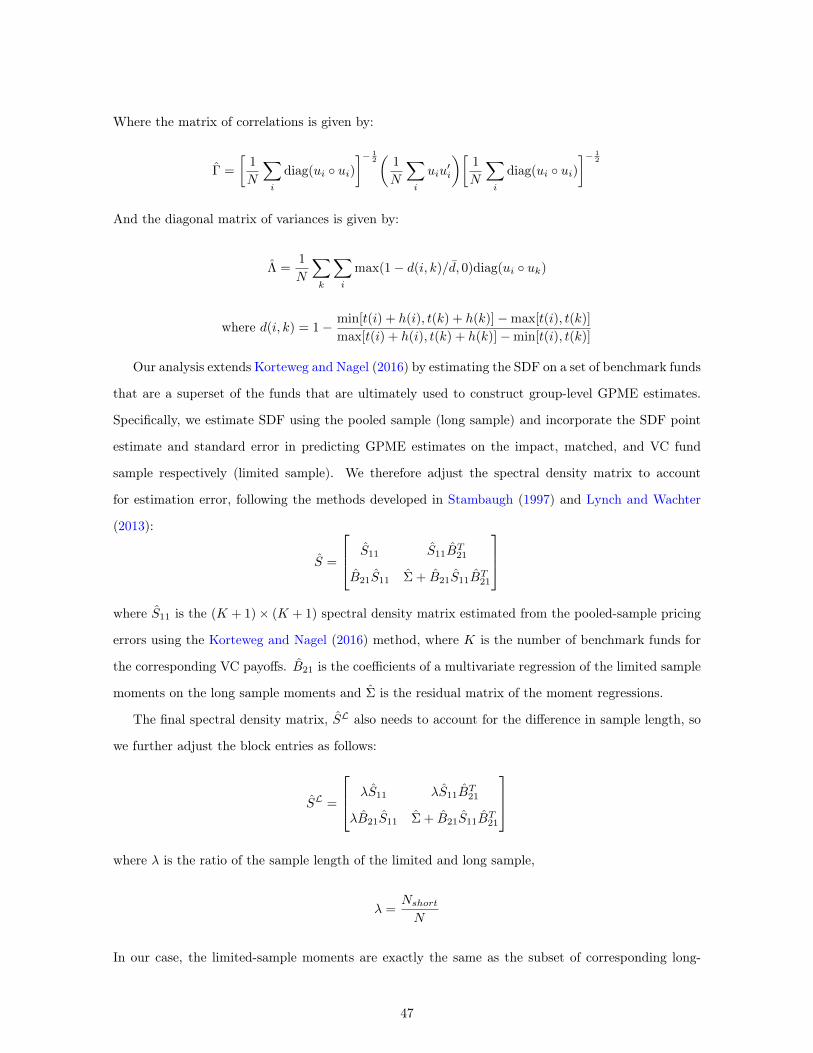
Where the matrix of correlations is given by:

Γ =

[1

N

∑i

diag(ui ◦ ui)]− 1

2(

1

N

∑i

uiu′i

)[1

N

∑i

diag(ui ◦ ui)]− 1

2

And the diagonal matrix of variances is given by:

Λ =1

N

∑k

∑i

max(1− d(i, k)/d, 0)diag(ui ◦ uk)

where d(i, k) = 1− min[t(i) + h(i), t(k) + h(k)]−max[t(i), t(k)]

max[t(i) + h(i), t(k) + h(k)]−min[t(i), t(k)]

Our analysis extends Korteweg and Nagel (2016) by estimating the SDF on a set of benchmark funds

that are a superset of the funds that are ultimately used to construct group-level GPME estimates.

Specifically, we estimate SDF using the pooled sample (long sample) and incorporate the SDF point

estimate and standard error in predicting GPME estimates on the impact, matched, and VC fund

sample respectively (limited sample). We therefore adjust the spectral density matrix to account

for estimation error, following the methods developed in Stambaugh (1997) and Lynch and Wachter

(2013):

S =

S11 S11BT21

B21S11 Σ + B21S11BT21

where S11 is the (K + 1)× (K + 1) spectral density matrix estimated from the pooled-sample pricing

errors using the Korteweg and Nagel (2016) method, where K is the number of benchmark funds for

the corresponding VC payoffs. B21 is the coefficients of a multivariate regression of the limited sample

moments on the long sample moments and Σ is the residual matrix of the moment regressions.

The final spectral density matrix, SL also needs to account for the difference in sample length, so

we further adjust the block entries as follows:

SL =

λS11 λS11BT21

λB21S11 Σ + B21S11BT21

where λ is the ratio of the sample length of the limited and long sample,

λ =NshortN

In our case, the limited-sample moments are exactly the same as the subset of corresponding long-

47

sample moments, since the long sample is the super-set of funds in the limited sample. Therefore, we

have

B21 =

1 0 0

0 1 0

0 0 1

The resulting adjusted spectral density matrix SL is a (2K + 2) × (2K + 2) matrix, including the

moments from VC payoff and benchmark payoffs from both the long and limited sample.

Note that, we do not need to use the efficient estimators developed by Lynch and Wachter (2013)

as we are using a pre-specified weighting matrix instead of the optimal weighting matrix W = S−1.

Thus, the variance of moment conditions is

var(g) = (I − d(d′Wd)−1d′W )S(I −Wd(d′Wd)−1d′)

where W is a (2K + 2)× (2K + 2) zero matrix with diagonal entries of 1 for corresponding benchmark

fund payoffs of the pooled sample, which are the only moments used to estimate the SDF. And a J-test

on GPME is

gV Cvar(gV C)−1gV C ∼ χ2(1)

48

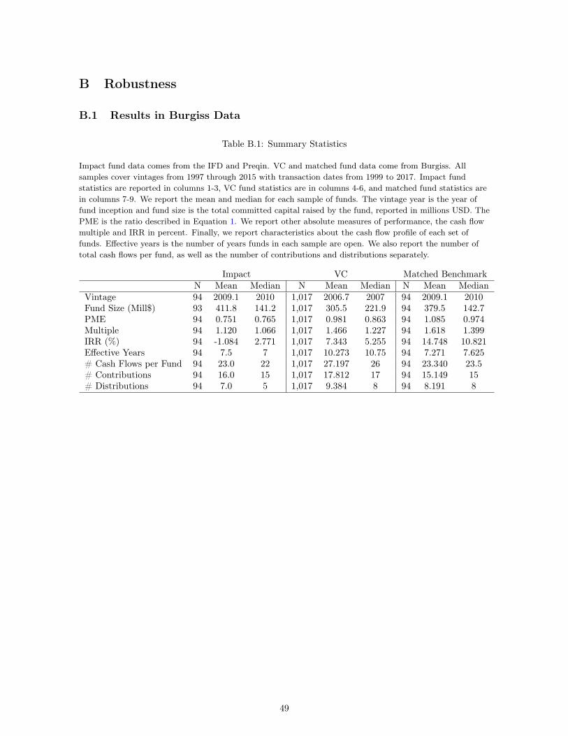
B Robustness

B.1 Results in Burgiss Data

Table B.1: Summary Statistics

Impact fund data comes from the IFD and Preqin. VC and matched fund data come from Burgiss. Allsamples cover vintages from 1997 through 2015 with transaction dates from 1999 to 2017. Impact fundstatistics are reported in columns 1-3, VC fund statistics are in columns 4-6, and matched fund statistics arein columns 7-9. We report the mean and median for each sample of funds. The vintage year is the year offund inception and fund size is the total committed capital raised by the fund, reported in millions USD. ThePME is the ratio described in Equation 1. We report other absolute measures of performance, the cash flowmultiple and IRR in percent. Finally, we report characteristics about the cash flow profile of each set offunds. Effective years is the number of years funds in each sample are open. We also report the number oftotal cash flows per fund, as well as the number of contributions and distributions separately.

Impact VC Matched BenchmarkN Mean Median N Mean Median N Mean Median

Vintage 94 2009.1 2010 1,017 2006.7 2007 94 2009.1 2010Fund Size (Mill$) 93 411.8 141.2 1,017 305.5 221.9 94 379.5 142.7PME 94 0.751 0.765 1,017 0.981 0.863 94 1.085 0.974Multiple 94 1.120 1.066 1,017 1.466 1.227 94 1.618 1.399IRR (%) 94 -1.084 2.771 1,017 7.343 5.255 94 14.748 10.821Effective Years 94 7.5 7 1,017 10.273 10.75 94 7.271 7.625# Cash Flows per Fund 94 23.0 22 1,017 27.197 26 94 23.340 23.5# Contributions 94 16.0 15 1,017 17.812 17 94 15.149 15# Distributions 94 7.0 5 1,017 9.384 8 94 8.191 8

49

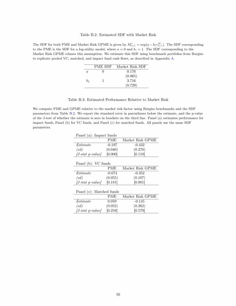
Table B.2: Estimated SDF with Market Risk

The SDF for both PME and Market Risk GPME is given by M∗t+1 = exp(a− b1rMt+1). The SDF correspondingto the PME is the SDF for a log-utility model, where a = 0 and b1 = 1. The SDF corresponding to theMarket Risk GPME relaxes this assumption. We estimate this SDF using benchmark portfolios from Burgissto replicate pooled VC, matched, and impact fund cash flows, as described in Appendix A.

PME SDF Market Risk SDFa 0 0.176

(0.065)b1 1 3.716

(0.729)

Table B.3: Estimated Performance Relative to Market Risk

We compute PME and GPME relative to the market risk factor using Burgiss benchmarks and the SDFparameters from Table B.2. We report the standard error in parentheses below the estimate, and the p-valueof the J-test of whether the estimate is zero in brackets on the third line. Panel (a) estimates performance forimpact funds, Panel (b) for VC funds, and Panel (c) for matched funds. All panels use the same SDFparameters.

Panel (a): Impact fundsPME Market Risk GPME

Estimate -0.197 -0.432(sd) (0.040) (0.270)[J-stat p-value] [0.000] [0.110]

Panel (b): VC fundsPME Market Risk GPME

Estimate -0.074 -0.352(sd) (0.055) (0.107)[J-stat p-value] [0.181] [0.001]

Panel (c): Matched fundsPME Market Risk GPME

Estimate 0.059 -0.145(sd) (0.052) (0.262)[J-stat p-value] [0.258] [0.579]

50

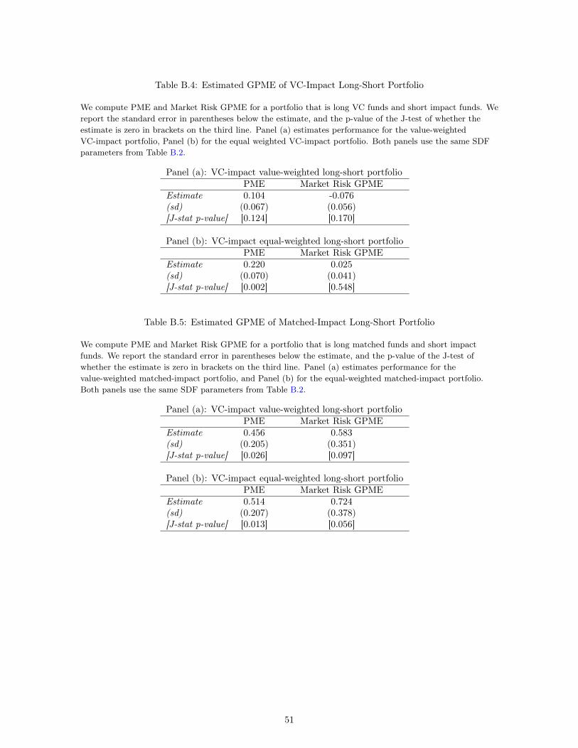
Table B.4: Estimated GPME of VC-Impact Long-Short Portfolio

We compute PME and Market Risk GPME for a portfolio that is long VC funds and short impact funds. Wereport the standard error in parentheses below the estimate, and the p-value of the J-test of whether theestimate is zero in brackets on the third line. Panel (a) estimates performance for the value-weightedVC-impact portfolio, Panel (b) for the equal weighted VC-impact portfolio. Both panels use the same SDFparameters from Table B.2.

Panel (a): VC-impact value-weighted long-short portfolioPME Market Risk GPME

Estimate 0.104 -0.076(sd) (0.067) (0.056)[J-stat p-value] [0.124] [0.170]

Panel (b): VC-impact equal-weighted long-short portfolioPME Market Risk GPME

Estimate 0.220 0.025(sd) (0.070) (0.041)[J-stat p-value] [0.002] [0.548]

Table B.5: Estimated GPME of Matched-Impact Long-Short Portfolio

We compute PME and Market Risk GPME for a portfolio that is long matched funds and short impactfunds. We report the standard error in parentheses below the estimate, and the p-value of the J-test ofwhether the estimate is zero in brackets on the third line. Panel (a) estimates performance for thevalue-weighted matched-impact portfolio, and Panel (b) for the equal-weighted matched-impact portfolio.Both panels use the same SDF parameters from Table B.2.

Panel (a): VC-impact value-weighted long-short portfolioPME Market Risk GPME

Estimate 0.456 0.583(sd) (0.205) (0.351)[J-stat p-value] [0.026] [0.097]

Panel (b): VC-impact equal-weighted long-short portfolioPME Market Risk GPME

Estimate 0.514 0.724(sd) (0.207) (0.378)[J-stat p-value] [0.013] [0.056]

51

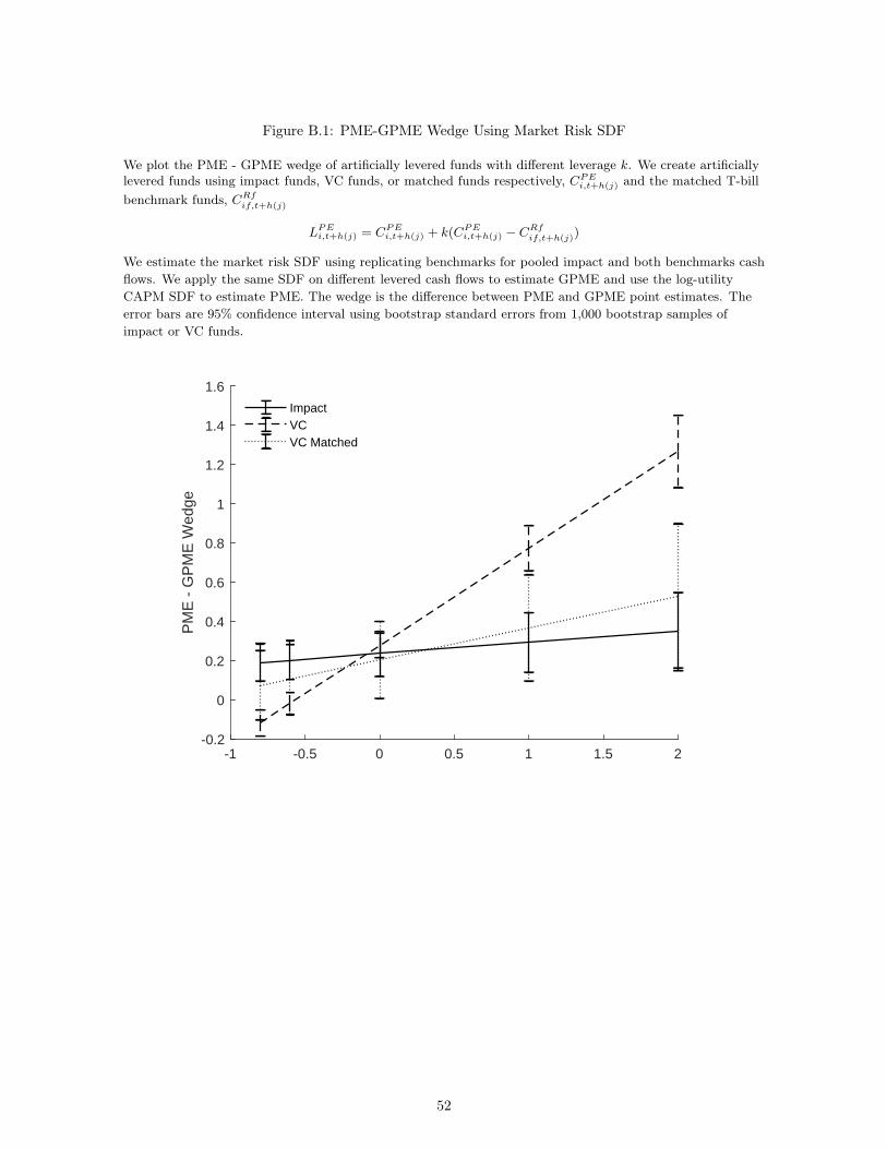
Figure B.1: PME-GPME Wedge Using Market Risk SDF

We plot the PME - GPME wedge of artificially levered funds with different leverage k. We create artificiallylevered funds using impact funds, VC funds, or matched funds respectively, CPE

i,t+h(j) and the matched T-billbenchmark funds, CRf

if,t+h(j)

LPEi,t+h(j) = CPE

i,t+h(j) + k(CPEi,t+h(j) − CRf

if,t+h(j))

We estimate the market risk SDF using replicating benchmarks for pooled impact and both benchmarks cashflows. We apply the same SDF on different levered cash flows to estimate GPME and use the log-utilityCAPM SDF to estimate PME. The wedge is the difference between PME and GPME point estimates. Theerror bars are 95% confidence interval using bootstrap standard errors from 1,000 bootstrap samples ofimpact or VC funds.

-1 -0.5 0 0.5 1 1.5 2-0.2

0

0.2

0.4

0.6

0.8

1

1.2

1.4

1.6

PM

E -

GP

ME

Wed

ge

ImpactVCVC Matched

52

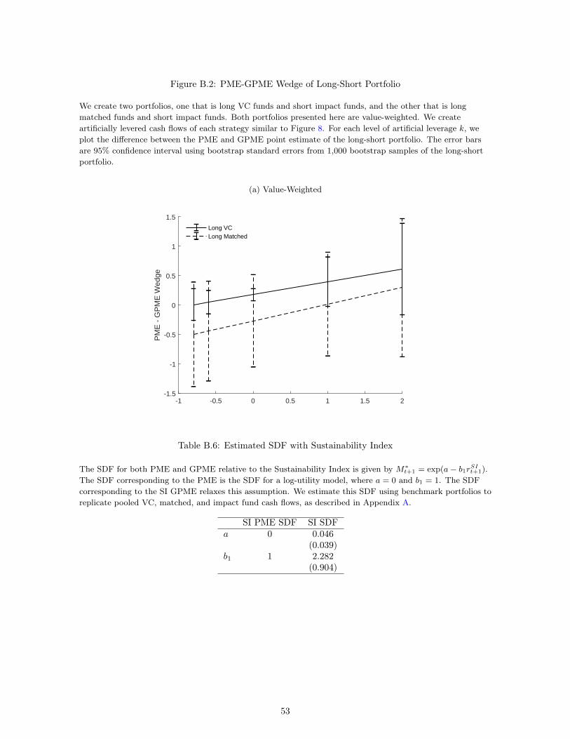
Figure B.2: PME-GPME Wedge of Long-Short Portfolio

We create two portfolios, one that is long VC funds and short impact funds, and the other that is longmatched funds and short impact funds. Both portfolios presented here are value-weighted. We createartificially levered cash flows of each strategy similar to Figure 8. For each level of artificial leverage k, weplot the difference between the PME and GPME point estimate of the long-short portfolio. The error barsare 95% confidence interval using bootstrap standard errors from 1,000 bootstrap samples of the long-shortportfolio.

(a) Value-Weighted

-1 -0.5 0 0.5 1 1.5 2-1.5

-1

-0.5

0

0.5

1

1.5

PM

E -

GP

ME

Wed

ge

Long VCLong Matched

Table B.6: Estimated SDF with Sustainability Index

The SDF for both PME and GPME relative to the Sustainability Index is given by M∗t+1 = exp(a− b1rSIt+1).

The SDF corresponding to the PME is the SDF for a log-utility model, where a = 0 and b1 = 1. The SDFcorresponding to the SI GPME relaxes this assumption. We estimate this SDF using benchmark portfolios toreplicate pooled VC, matched, and impact fund cash flows, as described in Appendix A.

SI PME SDF SI SDFa 0 0.046

(0.039)b1 1 2.282

(0.904)

53

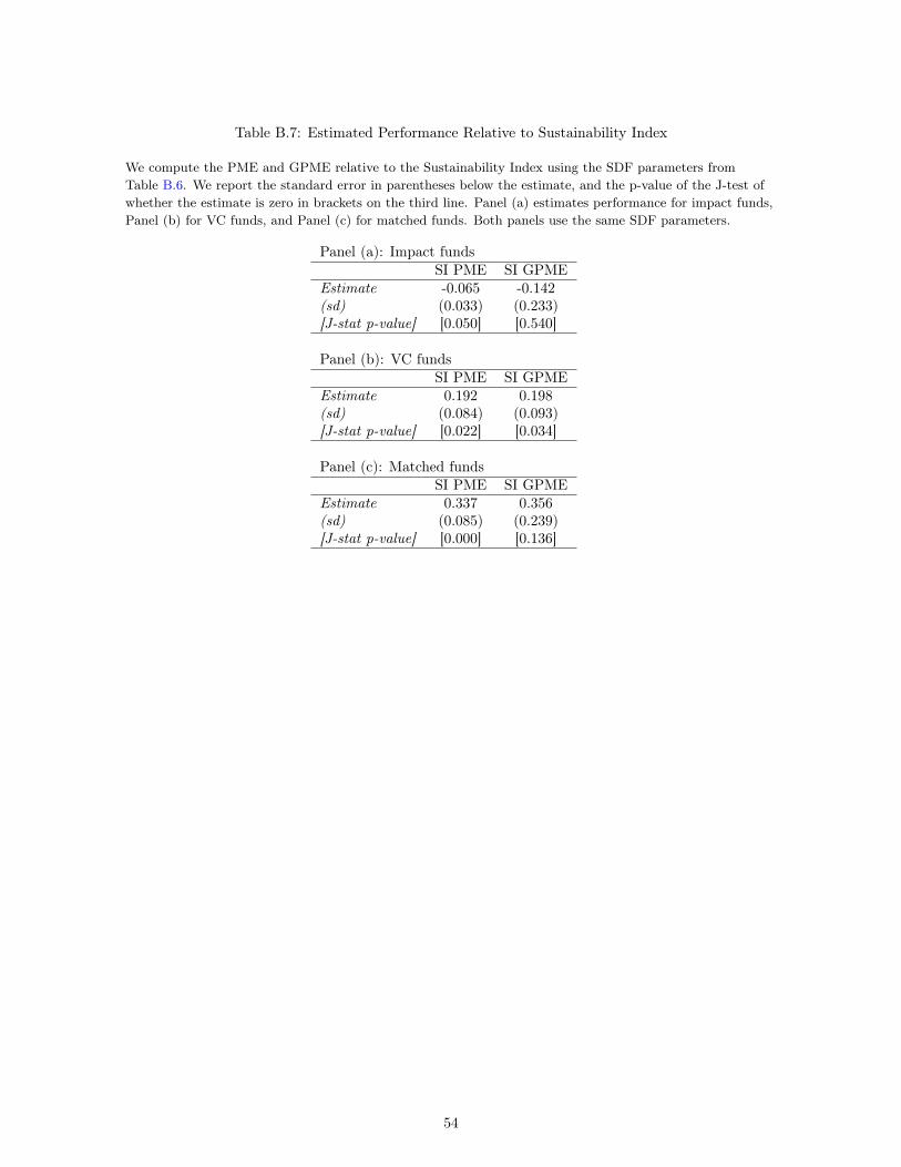
Table B.7: Estimated Performance Relative to Sustainability Index

We compute the PME and GPME relative to the Sustainability Index using the SDF parameters fromTable B.6. We report the standard error in parentheses below the estimate, and the p-value of the J-test ofwhether the estimate is zero in brackets on the third line. Panel (a) estimates performance for impact funds,Panel (b) for VC funds, and Panel (c) for matched funds. Both panels use the same SDF parameters.

Panel (a): Impact fundsSI PME SI GPME

Estimate -0.065 -0.142(sd) (0.033) (0.233)[J-stat p-value] [0.050] [0.540]

Panel (b): VC fundsSI PME SI GPME

Estimate 0.192 0.198(sd) (0.084) (0.093)[J-stat p-value] [0.022] [0.034]

Panel (c): Matched fundsSI PME SI GPME

Estimate 0.337 0.356(sd) (0.085) (0.239)[J-stat p-value] [0.000] [0.136]

54

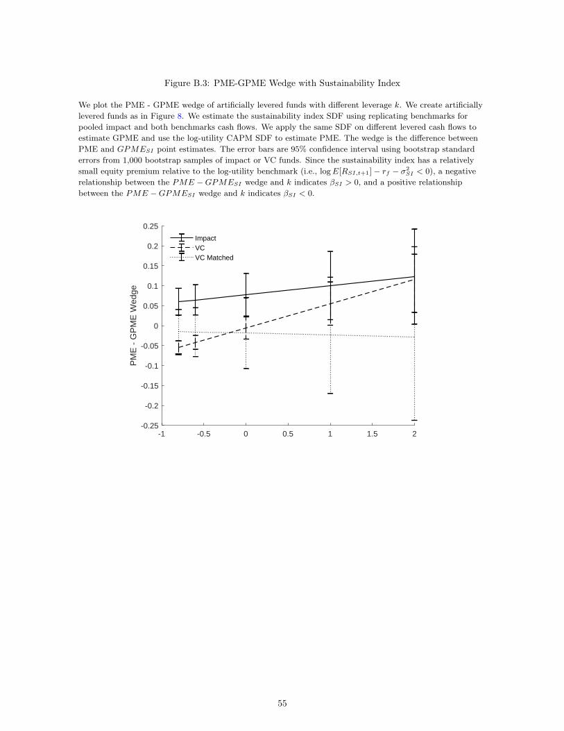
Figure B.3: PME-GPME Wedge with Sustainability Index

We plot the PME - GPME wedge of artificially levered funds with different leverage k. We create artificiallylevered funds as in Figure 8. We estimate the sustainability index SDF using replicating benchmarks forpooled impact and both benchmarks cash flows. We apply the same SDF on different levered cash flows toestimate GPME and use the log-utility CAPM SDF to estimate PME. The wedge is the difference betweenPME and GPMESI point estimates. The error bars are 95% confidence interval using bootstrap standarderrors from 1,000 bootstrap samples of impact or VC funds. Since the sustainability index has a relativelysmall equity premium relative to the log-utility benchmark (i.e., logE[RSI,t+1]− rf − σ2

SI < 0), a negativerelationship between the PME −GPMESI wedge and k indicates βSI > 0, and a positive relationshipbetween the PME −GPMESI wedge and k indicates βSI < 0.

-1 -0.5 0 0.5 1 1.5 2-0.25

-0.2

-0.15

-0.1

-0.05

0

0.05

0.1

0.15

0.2

0.25

PM

E -

GP

ME

Wed

ge

ImpactVCVC Matched

55

Table B.8: GPME with Multi-Factor SDF

We compute the GPME for different factor models: one-factor model with market factor only, two-factormodel with market and small growth, and two-factor model with market and sustainability index. We reportthe standard error in parentheses below the estimate, and the p-value of the J-test of whether the estimate iszero in brackets on the third line. Panel (a) estimates performance for impact funds, Panel (b) for VC funds,and Panel (c) for matched funds. Both panels use the same SDF parameters; each column has its own set ofSDF parameters corresponding to the relevant model.

Panel (a): Impact fundsMarket Factor Market and Market and

Only Small Growth SustainabilityEstimate -0.432 -0.415 -0.327(sd) (0.270) (0.239) (0.544)[J-stat p-value] [0.110] [0.082] [0.548]

Panel (b): VC fundsMarket Factor Market and Market and

Only Small Growth SustainabilityEstimate -0.352 -0.332 -0.433(sd) (0.107) (0.096) (0.163)[J-stat p-value] [0.001] [0.001] [0.008]

Panel (c): Matched fundsMarket Factor Market and Market and

Only Small Growth SustainabilityEstimate -0.145 -0.108 -0.237(sd) (0.262) (0.239) (0.541)[J-stat p-value] [0.579] [0.651] [0.662]

B.2 Matched Benchmark by Asset Class, Vintage, Sequence Number, and

Size

In our main analysis, we construct our matched benchmark by matching each impact fund to a

fund in Preqin with the same vintage and general asset class, and closest size. In this section, we

perform an alternative matching process in order to address the concern that some of the performance

differences of impact funds compared to our benchmarks are due to the fact that impact funds are

relatively new, that is they are early in their fund sequence. In particular, we match on the same

vintage and general asset class, and closest sequence number and size. We does not match exactly on

sequence number because there are not always some Preqin funds with the exact same vintage, asset

class and sequence number as each impact fund in our sample.

The last three columns of Table B.9 show the summary statistics of the selected funds with this

alternative matching procedure. The matched funds have almost identical sequence number distribu-

tion as impact funds, even if we are not matching exactly on sequence number. The size difference

56

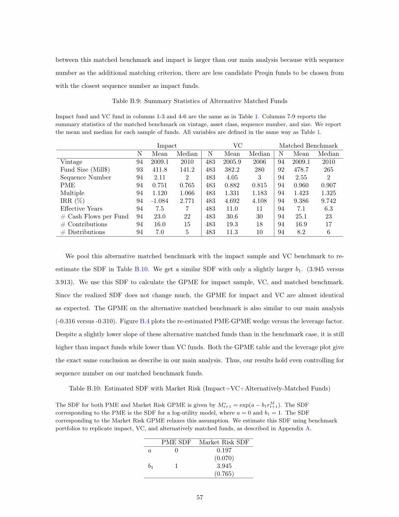
between this matched benchmark and impact is larger than our main analysis because with sequence

number as the additional matching criterion, there are less candidate Preqin funds to be chosen from

with the closest sequence number as impact funds.

Table B.9: Summary Statistics of Alternative Matched Funds

Impact fund and VC fund in columns 1-3 and 4-6 are the same as in Table 1. Columns 7-9 reports thesummary statistics of the matched benchmark on vintage, asset class, sequence number, and size. We reportthe mean and median for each sample of funds. All variables are defined in the same way as Table 1.

Impact VC Matched BenchmarkN Mean Median N Mean Median N Mean Median

Vintage 94 2009.1 2010 483 2005.9 2006 94 2009.1 2010Fund Size (Mill$) 93 411.8 141.2 483 382.2 280 92 478.7 265Sequence Number 94 2.11 2 483 4.05 3 94 2.55 2PME 94 0.751 0.765 483 0.882 0.815 94 0.960 0.907Multiple 94 1.120 1.066 483 1.331 1.183 94 1.423 1.325IRR (%) 94 -1.084 2.771 483 4.692 4.108 94 9.386 9.742Effective Years 94 7.5 7 483 11.0 11 94 7.1 6.3# Cash Flows per Fund 94 23.0 22 483 30.6 30 94 25.1 23# Contributions 94 16.0 15 483 19.3 18 94 16.9 17# Distributions 94 7.0 5 483 11.3 10 94 8.2 6

We pool this alternative matched benchmark with the impact sample and VC benchmark to re-

estimate the SDF in Table B.10. We get a similar SDF with only a slightly larger b1. (3.945 versus

3.913). We use this SDF to calculate the GPME for impact sample, VC, and matched benchmark.

Since the realized SDF does not change much, the GPME for impact and VC are almost identical

as expected. The GPME on the alternative matched benchmark is also similar to our main analysis

(-0.316 versus -0.310). Figure B.4 plots the re-estimated PME-GPME wedge versus the leverage factor.

Despite a slightly lower slope of these alternative matched funds than in the benchmark case, it is still

higher than impact funds while lower than VC funds. Both the GPME table and the leverage plot give

the exact same conclusion as describe in our main analysis. Thus, our results hold even controlling for

sequence number on our matched benchmark funds.

Table B.10: Estimated SDF with Market Risk (Impact+VC+Alternatively-Matched Funds)

The SDF for both PME and Market Risk GPME is given by M∗t+1 = exp(a− b1rMt+1). The SDF

corresponding to the PME is the SDF for a log-utility model, where a = 0 and b1 = 1. The SDFcorresponding to the Market Risk GPME relaxes this assumption. We estimate this SDF using benchmarkportfolios to replicate impact, VC, and alternatively matched funds, as described in Appendix A.

PME SDF Market Risk SDFa 0 0.197

(0.070)b1 1 3.945

(0.765)

57

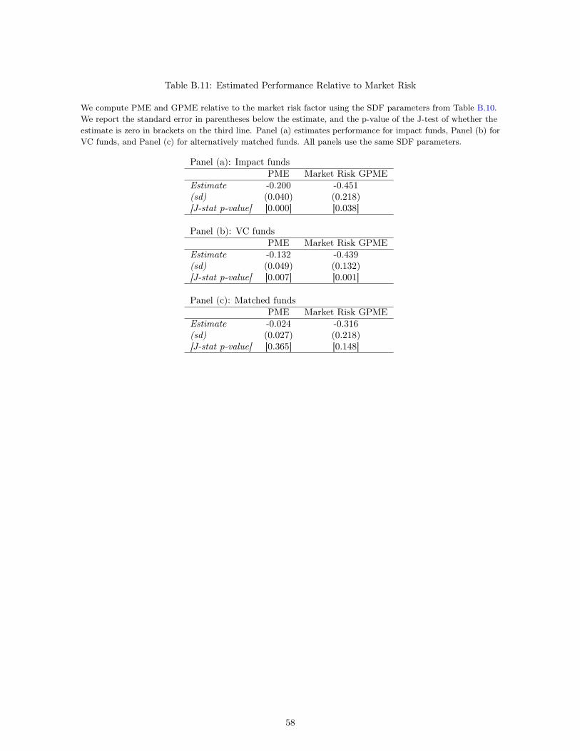
Table B.11: Estimated Performance Relative to Market Risk

We compute PME and GPME relative to the market risk factor using the SDF parameters from Table B.10.We report the standard error in parentheses below the estimate, and the p-value of the J-test of whether theestimate is zero in brackets on the third line. Panel (a) estimates performance for impact funds, Panel (b) forVC funds, and Panel (c) for alternatively matched funds. All panels use the same SDF parameters.

Panel (a): Impact fundsPME Market Risk GPME

Estimate -0.200 -0.451(sd) (0.040) (0.218)[J-stat p-value] [0.000] [0.038]

Panel (b): VC fundsPME Market Risk GPME

Estimate -0.132 -0.439(sd) (0.049) (0.132)[J-stat p-value] [0.007] [0.001]

Panel (c): Matched fundsPME Market Risk GPME

Estimate -0.024 -0.316(sd) (0.027) (0.218)[J-stat p-value] [0.365] [0.148]

58

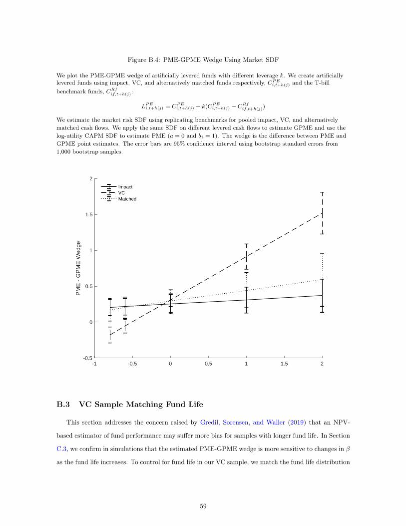
Figure B.4: PME-GPME Wedge Using Market SDF

We plot the PME-GPME wedge of artificially levered funds with different leverage k. We create artificiallylevered funds using impact, VC, and alternatively matched funds respectively, CPE

i,t+h(j) and the T-billbenchmark funds, CRf

if,t+h(j):

LPEi,t+h(j) = CPE

i,t+h(j) + k(CPEi,t+h(j) − CRf

if,t+h(j))

We estimate the market risk SDF using replicating benchmarks for pooled impact, VC, and alternativelymatched cash flows. We apply the same SDF on different levered cash flows to estimate GPME and use thelog-utility CAPM SDF to estimate PME (a = 0 and b1 = 1). The wedge is the difference between PME andGPME point estimates. The error bars are 95% confidence interval using bootstrap standard errors from1,000 bootstrap samples.

-1 -0.5 0 0.5 1 1.5 2-0.5

0

0.5

1

1.5

2

PM

E -

GP

ME

Wed

ge

ImpactVCMatched

B.3 VC Sample Matching Fund Life

This section addresses the concern raised by Gredil, Sorensen, and Waller (2019) that an NPV-

based estimator of fund performance may suffer more bias for samples with longer fund life. In Section

C.3, we confirm in simulations that the estimated PME-GPME wedge is more sensitive to changes in β

as the fund life increases. To control for fund life in our VC sample, we match the fund life distribution

59

of our VC benchmark sample to our impact sample and re-estimate the PME and GPMEs.10 We take

a two-step process to match the fund life distribution: (i) we match the vintage distribution of the VC

sample to the vintage distribution of our impact sample by keeping all of the VC funds in the most

populated impact vintage year (2010), and then randomly drop VC funds in other vintage years in

proportion to the impact vintage distribution; (ii) for each vintage year, we cut off VC fund cash flows

at the mean impact fund life within that year. The last three columns of Table B.12 show the summary

statistics of the VC sample matched by fund life. We can see that while maintaining similar size as

the full VC sample, this matched sample follows closely the vintage and effective years distribution of

the impact fund sample.

Table B.12: Summary Statistics of VC Matched by Fund Life

Impact fund and VC fund in columns 1-3 and 4-6 are the same as in Table 1. Columns 7-9 reports thesummary statistics of the fund-life-matched sample constructed by the process described above. We reportthe mean and median for each sample of funds. All variables are defined in the same way as Table 1.

Impact Funds All VC Funds VC Matched by Fund LifeN Mean Median N Mean Median N Mean Median

Vintage 51 2009.5 2010 483 2005.9 2006 144 2009.4 2010Fund Size (Mill$) 51 95.3 74.4 483 382.2 280 144 370.0 286PME 51 0.777 0.767 483 0.882 0.815 144 1.002 0.933

Multiple 51 1.123 1.081 483 1.331 1.183 144 1.429 1.274IRR (%) 51 1.526 3.327 483 4.692 4.108 144 12.42 9.328Effective Years 51 6.7 6.0 483 11.0 11 144 6.5 5.8# Cash Flows per Fund 51 18.7 16 483 30.6 30 144 23.0 21# Contributions 51 13.3 12 483 19.3 18 144 16.0 16# Distributions 51 5.4 2 483 11.3 10 144 7.0 5

We pool the fund-life-matched VC sample with the IFD impact sample and re-estimate the SDF in

Table B.13. Despite having a larger b1, the SDF is consistent with the relatively “hot” equity markets

in our main results. In Figure B.5, we plot the re-estimated PME-GPME wedge as a function of the

artificial leverage factor, separately for fund-life-matched VC and impact funds. There is still a much

higher slope for the matched VC funds, suggesting that impact funds have a lower β than VC even

after controlling for fund life. This confirms and strengthens our main results that impact funds have

a substantially lower market beta than venture capital funds.10This robustness test was conducted with the original sample of 51 impact funds. We are working on repeating this

for the expanded sample of 94 impact funds.

60

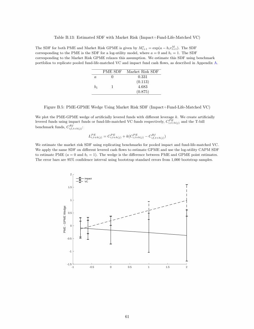
Table B.13: Estimated SDF with Market Risk (Impact+Fund-Life-Matched VC)

The SDF for both PME and Market Risk GPME is given by M∗t+1 = exp(a− b1rMt+1). The SDF

corresponding to the PME is the SDF for a log-utility model, where a = 0 and b1 = 1. The SDFcorresponding to the Market Risk GPME relaxes this assumption. We estimate this SDF using benchmarkportfolios to replicate pooled fund-life-matched VC and impact fund cash flows, as described in Appendix A.

PME SDF Market Risk SDFa 0 0.331

(0.113)b1 1 4.683

(0.875)

Figure B.5: PME-GPME Wedge Using Market Risk SDF (Impact+Fund-Life-Matched VC)

We plot the PME-GPME wedge of artificially levered funds with different leverage k. We create artificiallylevered funds using impact funds or fund-life-matched VC funds respectively, CPE

i,t+h(j) and the T-billbenchmark funds, CRf

if,t+h(j):

LPEi,t+h(j) = CPE

i,t+h(j) + k(CPEi,t+h(j) − CRf

if,t+h(j))

We estimate the market risk SDF using replicating benchmarks for pooled impact and fund-life-matched VC.We apply the same SDF on different levered cash flows to estimate GPME and use the log-utility CAPM SDFto estimate PME (a = 0 and b1 = 1). The wedge is the difference between PME and GPME point estimates.The error bars are 95% confidence interval using bootstrap standard errors from 1,000 bootstrap samples.

-1 -0.5 0 0.5 1 1.5 2-1.5

-1

-0.5

0

0.5

1

1.5

2

PM

E -

GP

ME

Wed

ge

ImpactVC

61

C Simulations

C.1 Finite-Sample Performance of PME-GPME Wedge

Our main result uses the difference in the PME-GPME wedge between impact and VC funds as

an indication of their difference in β. As stated in Section 3.3, this method is based on the following

equation:

logE[RGPME ]− logE[RPME ] = (β − 1)(logE[Rm,t+1]− rf − σ2m) (15)

This equation shows that in true expectations, we can have a one-to-one relationship between the

PME-GPME wedge and β. However, the relationship is not exact when we estimate the wedge in

finite samples, especially in small samples like ours. In particular, our results depend on the fact that

the following relationship holds in the finite sample:

logE[RGPME ]− logE[RPME ] = f(PME −GPME) (16)

where f is an strictly increasing function.

We verify this relationship using Monte Carlo simulations. To create simulated fund cash flows, we

first assume that the log market return follows

ft = rf + γσ2 − 1

2σ2 + σεt (17)

where εt ∼ N(0, 1), rf is a constant log risk-free rate, γ is risk aversion coefficient, and V ar(ft) = σ2.

This specification guarantees that the log SDF with the form

mt = a− γft (18)

prices the risk-free rate and market factor perfectly in population, with a = (γ − 1)rf + 12γ(γ − 1)σ2.

We then model fund returns with any arbitrary β as

rt = rf + βγσ2 − 1

2β2σ2 + βσεt + ηt −

1

2ω2 (19)

One can easily show that such fund returns satisfy the definition of β:

β =Cov(rt, ft)

σ2=Cov(rt, σεt)

σ2(20)

62

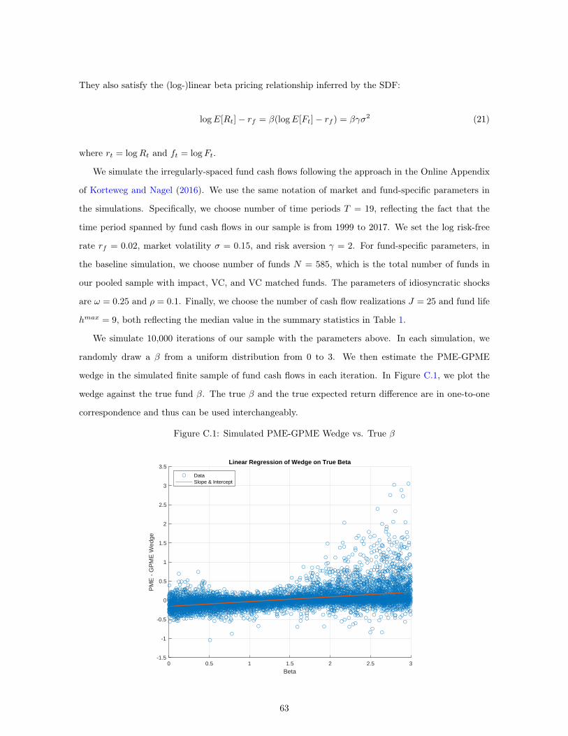
They also satisfy the (log-)linear beta pricing relationship inferred by the SDF:

logE[Rt]− rf = β(logE[Ft]− rf ) = βγσ2 (21)

where rt = logRt and ft = logFt.

We simulate the irregularly-spaced fund cash flows following the approach in the Online Appendix

of Korteweg and Nagel (2016). We use the same notation of market and fund-specific parameters in

the simulations. Specifically, we choose number of time periods T = 19, reflecting the fact that the

time period spanned by fund cash flows in our sample is from 1999 to 2017. We set the log risk-free

rate rf = 0.02, market volatility σ = 0.15, and risk aversion γ = 2. For fund-specific parameters, in

the baseline simulation, we choose number of funds N = 585, which is the total number of funds in

our pooled sample with impact, VC, and VC matched funds. The parameters of idiosyncratic shocks

are ω = 0.25 and ρ = 0.1. Finally, we choose the number of cash flow realizations J = 25 and fund life

hmax = 9, both reflecting the median value in the summary statistics in Table 1.

We simulate 10,000 iterations of our sample with the parameters above. In each simulation, we

randomly draw a β from a uniform distribution from 0 to 3. We then estimate the PME-GPME

wedge in the simulated finite sample of fund cash flows in each iteration. In Figure C.1, we plot the

wedge against the true fund β. The true β and the true expected return difference are in one-to-one

correspondence and thus can be used interchangeably.

Figure C.1: Simulated PME-GPME Wedge vs. True β

0 0.5 1 1.5 2 2.5 3

Beta

-1.5

-1

-0.5

0

0.5

1

1.5

2

2.5

3

3.5

PM

E -

GP

ME

Wed

ge

Linear Regression of Wedge on True Beta

DataSlope & Intercept

63

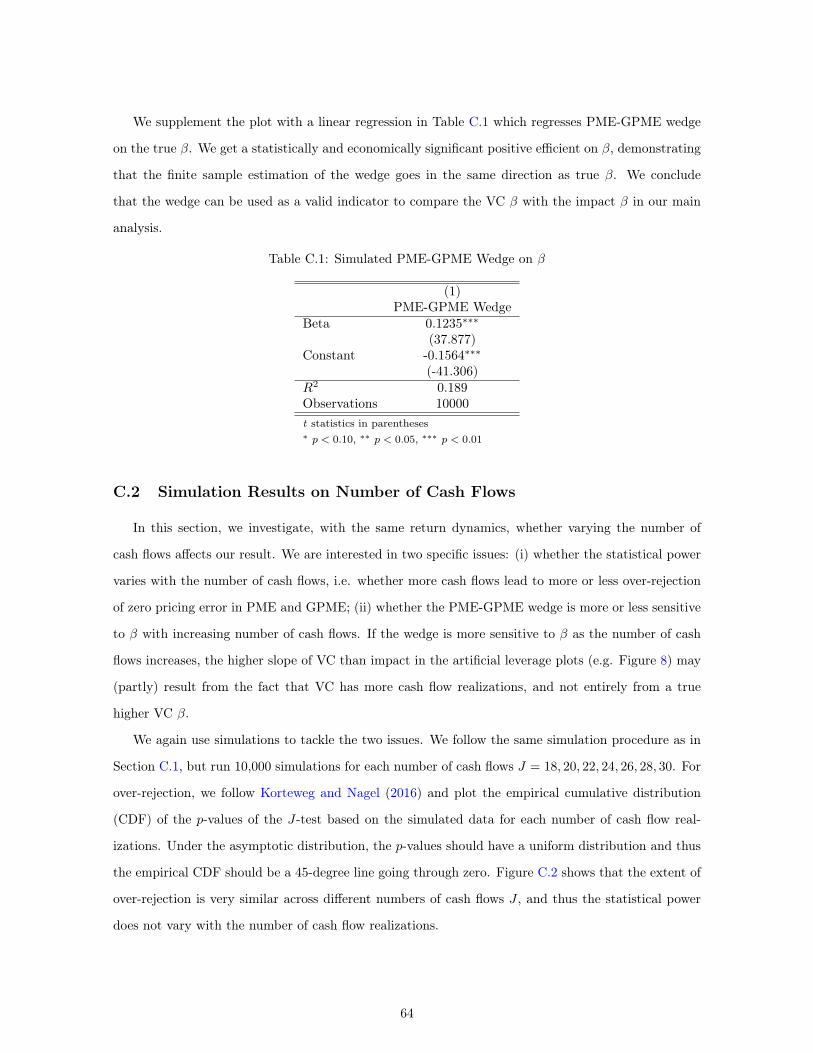
We supplement the plot with a linear regression in Table C.1 which regresses PME-GPME wedge

on the true β. We get a statistically and economically significant positive efficient on β, demonstrating

that the finite sample estimation of the wedge goes in the same direction as true β. We conclude

that the wedge can be used as a valid indicator to compare the VC β with the impact β in our main

analysis.

Table C.1: Simulated PME-GPME Wedge on β

(1)PME-GPME Wedge

Beta 0.1235∗∗∗(37.877)

Constant -0.1564∗∗∗(-41.306)

R2 0.189Observations 10000t statistics in parentheses∗ p < 0.10, ∗∗ p < 0.05, ∗∗∗ p < 0.01

C.2 Simulation Results on Number of Cash Flows

In this section, we investigate, with the same return dynamics, whether varying the number of

cash flows affects our result. We are interested in two specific issues: (i) whether the statistical power

varies with the number of cash flows, i.e. whether more cash flows lead to more or less over-rejection

of zero pricing error in PME and GPME; (ii) whether the PME-GPME wedge is more or less sensitive

to β with increasing number of cash flows. If the wedge is more sensitive to β as the number of cash

flows increases, the higher slope of VC than impact in the artificial leverage plots (e.g. Figure 8) may

(partly) result from the fact that VC has more cash flow realizations, and not entirely from a true

higher VC β.

We again use simulations to tackle the two issues. We follow the same simulation procedure as in

Section C.1, but run 10,000 simulations for each number of cash flows J = 18, 20, 22, 24, 26, 28, 30. For

over-rejection, we follow Korteweg and Nagel (2016) and plot the empirical cumulative distribution

(CDF) of the p-values of the J-test based on the simulated data for each number of cash flow real-

izations. Under the asymptotic distribution, the p-values should have a uniform distribution and thus

the empirical CDF should be a 45-degree line going through zero. Figure C.2 shows that the extent of

over-rejection is very similar across different numbers of cash flows J , and thus the statistical power

does not vary with the number of cash flow realizations.

64

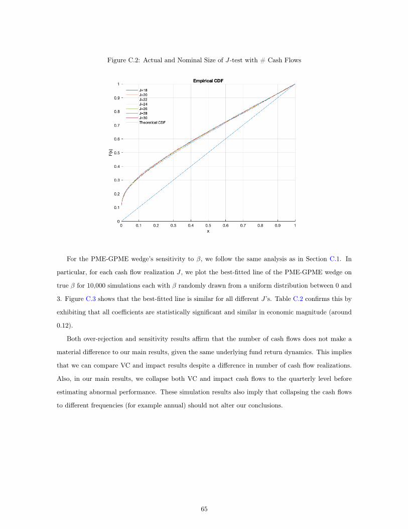
Figure C.2: Actual and Nominal Size of J-test with # Cash Flows

For the PME-GPME wedge’s sensitivity to β, we follow the same analysis as in Section C.1. In

particular, for each cash flow realization J , we plot the best-fitted line of the PME-GPME wedge on

true β for 10,000 simulations each with β randomly drawn from a uniform distribution between 0 and

3. Figure C.3 shows that the best-fitted line is similar for all different J ’s. Table C.2 confirms this by

exhibiting that all coefficients are statistically significant and similar in economic magnitude (around

0.12).

Both over-rejection and sensitivity results affirm that the number of cash flows does not make a

material difference to our main results, given the same underlying fund return dynamics. This implies

that we can compare VC and impact results despite a difference in number of cash flow realizations.

Also, in our main results, we collapse both VC and impact cash flows to the quarterly level before

estimating abnormal performance. These simulation results also imply that collapsing the cash flows

to different frequencies (for example annual) should not alter our conclusions.

65

Figure C.3: Simulated PME-GPME Wedge vs. True β with # Cash Flows

0 0.5 1 1.5 2 2.5 3

Beta

-0.2

-0.15

-0.1

-0.05

0

0.05

0.1

0.15

0.2

0.25

PM

E -

GP

ME

Wed

ge

J=18J=20J=22J=24J=26J=28J=30

Table C.2: PME-GPME Wedge on β with # Cash Flows

J 18 20 22 24 26 28 30Beta 0.1294∗∗∗ 0.1168∗∗∗ 0.1242∗∗∗ 0.1287∗∗∗ 0.1186∗∗∗ 0.1210∗∗∗ 0.1205∗∗∗

(38.724) (36.940) (35.430) (36.244) (36.257) (35.346) (36.499)Constant -0.1630∗∗∗ -0.1467∗∗∗ -0.1555∗∗∗ -0.1609∗∗∗ -0.1508∗∗∗ -0.1503∗∗∗ -0.1523∗∗∗

(-42.318) (-38.442) (-38.557) (-39.041) (-38.767) (-37.545) (-39.329)R2 0.200 0.184 0.173 0.182 0.181 0.175 0.176Observations 9,999 9,995 9,999 9,998 10,000 9,999 9,997t statistics in parentheses∗ p < 0.10, ∗∗ p < 0.05, ∗∗∗ p < 0.01

66

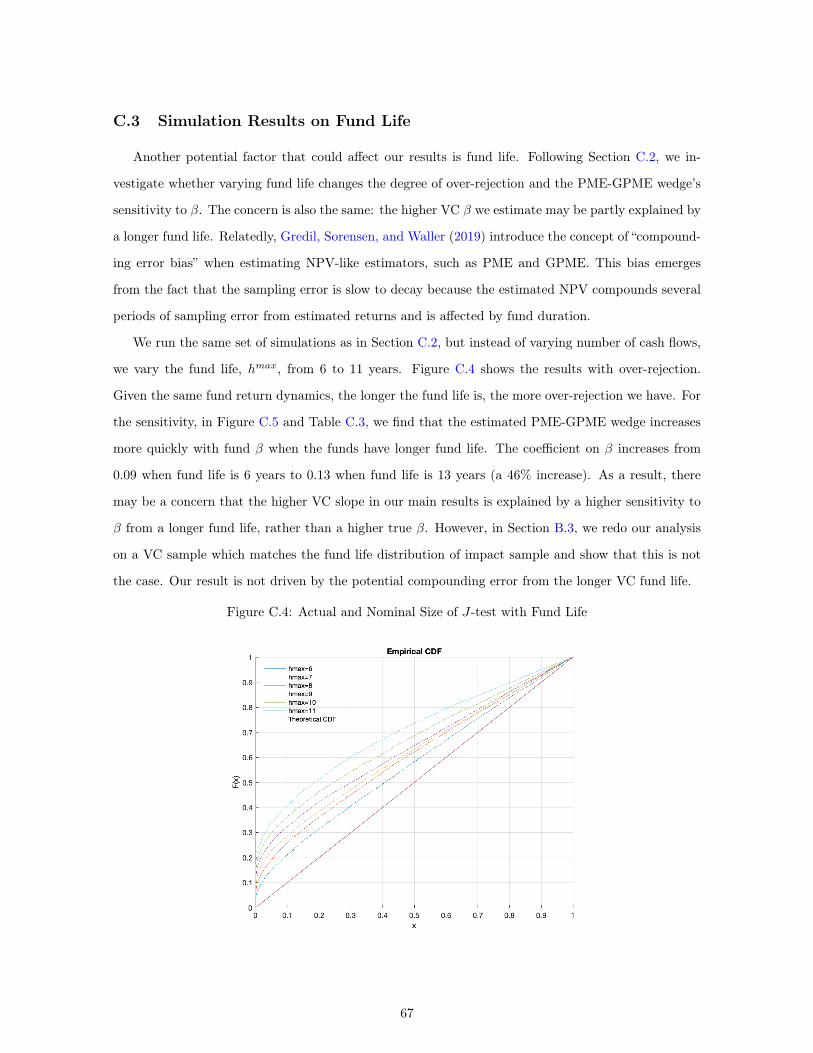
C.3 Simulation Results on Fund Life

Another potential factor that could affect our results is fund life. Following Section C.2, we in-

vestigate whether varying fund life changes the degree of over-rejection and the PME-GPME wedge’s

sensitivity to β. The concern is also the same: the higher VC β we estimate may be partly explained by

a longer fund life. Relatedly, Gredil, Sorensen, and Waller (2019) introduce the concept of “compound-

ing error bias” when estimating NPV-like estimators, such as PME and GPME. This bias emerges

from the fact that the sampling error is slow to decay because the estimated NPV compounds several

periods of sampling error from estimated returns and is affected by fund duration.

We run the same set of simulations as in Section C.2, but instead of varying number of cash flows,

we vary the fund life, hmax, from 6 to 11 years. Figure C.4 shows the results with over-rejection.

Given the same fund return dynamics, the longer the fund life is, the more over-rejection we have. For

the sensitivity, in Figure C.5 and Table C.3, we find that the estimated PME-GPME wedge increases

more quickly with fund β when the funds have longer fund life. The coefficient on β increases from

0.09 when fund life is 6 years to 0.13 when fund life is 13 years (a 46% increase). As a result, there

may be a concern that the higher VC slope in our main results is explained by a higher sensitivity to

β from a longer fund life, rather than a higher true β. However, in Section B.3, we redo our analysis

on a VC sample which matches the fund life distribution of impact sample and show that this is not

the case. Our result is not driven by the potential compounding error from the longer VC fund life.

Figure C.4: Actual and Nominal Size of J-test with Fund Life

67

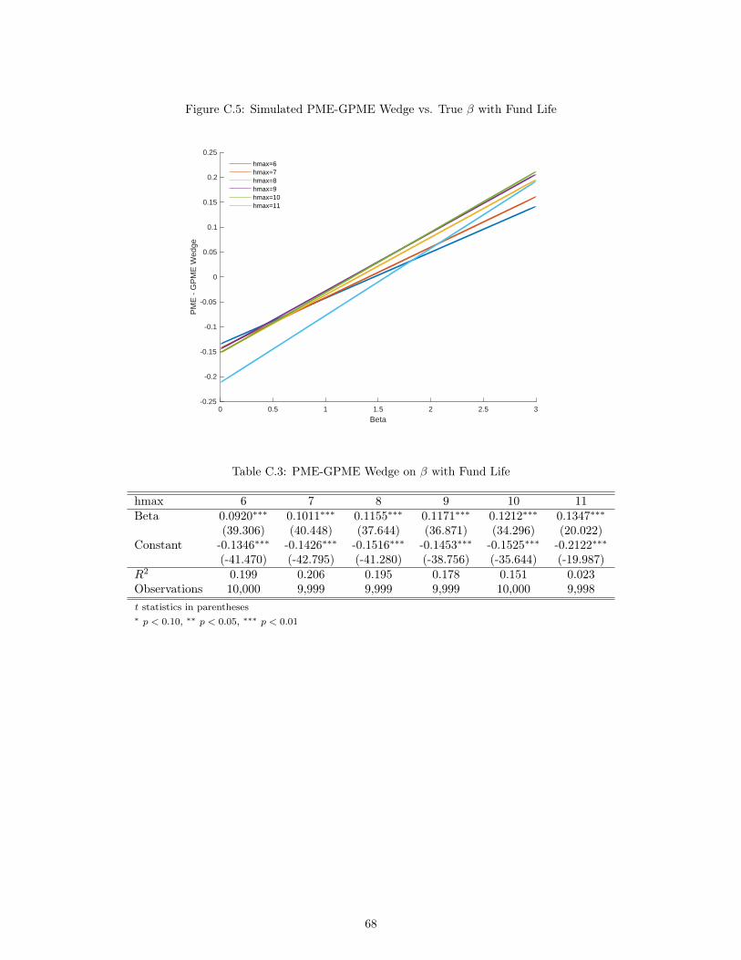
Figure C.5: Simulated PME-GPME Wedge vs. True β with Fund Life

0 0.5 1 1.5 2 2.5 3

Beta

-0.25

-0.2

-0.15

-0.1

-0.05

0

0.05

0.1

0.15

0.2

0.25

PM

E -

GP

ME

Wed

ge

hmax=6hmax=7hmax=8hmax=9hmax=10hmax=11

Table C.3: PME-GPME Wedge on β with Fund Life

hmax 6 7 8 9 10 11Beta 0.0920∗∗∗ 0.1011∗∗∗ 0.1155∗∗∗ 0.1171∗∗∗ 0.1212∗∗∗ 0.1347∗∗∗

(39.306) (40.448) (37.644) (36.871) (34.296) (20.022)Constant -0.1346∗∗∗ -0.1426∗∗∗ -0.1516∗∗∗ -0.1453∗∗∗ -0.1525∗∗∗ -0.2122∗∗∗

(-41.470) (-42.795) (-41.280) (-38.756) (-35.644) (-19.987)R2 0.199 0.206 0.195 0.178 0.151 0.023Observations 10,000 9,999 9,999 9,999 10,000 9,998t statistics in parentheses∗ p < 0.10, ∗∗ p < 0.05, ∗∗∗ p < 0.01

68