The Rise of Multiprecision Computationshigham/talks/arith17.pdf · Research Matters February 25,...

Research Matters

February 25, 2009

Nick HighamDirector of Research

School of Mathematics

1 / 6

The Rise of MultiprecisionComputations

Nick HighamSchool of Mathematics

The University of Manchester

http://www.ma.man.ac.uk/~higham@nhigham, nickhigham.wordpress.com

24th IEEE Symposium on Computer Arithmetic,London, July 24–26, 2017

http://www.manchester.ac.uk

http://www.maths.manchester.ac.uk/our-research/research-groups/numerical-analysis-and-scientific-computing/numerical-analysis/

http://www.ma.man.ac.uk/~higham/

http://www.ma.man.ac.uk

http://www.man.ac.uk

http://www.ma.man.ac.uk/~higham/

https://twitter.com/nhigham

http://nickhigham.wordpress.com

Outline

Multiprecision arithmetic: floating point arithmeticsupporting multiple, possibly arbitrary, precisions.

Applications of & support for low precision.

Applications of & support for high precision.

How to exploit different precisions to achieve faster algswith higher accuracy.

Focus on iterative refinement for Ax = b.

Download this talk fromhttp://bit.ly/higham-arith24

Nick Higham The Rise of Multiprecision Computations 2 / 48

http://bit.ly/higham-samsi17

IEEE Standard 754-1985 and 2008 Revision

Type Size Range u = 2−t

half 16 bits 10±5 2−11 ≈ 4.9× 10−4

single 32 bits 10±38 2−24 ≈ 6.0× 10−8

double 64 bits 10±308 2−53 ≈ 1.1× 10−16

quadruple 128 bits 10±4932 2−113 ≈ 9.6× 10−35

Arithmetic ops (+,−, ∗, /,√) performed as if firstcalculated to infinite precision, then rounded.Default: round to nearest, round to even in case of tie.Half precision is a storage format only.


Intel Core Family (3rd gen., 2012)

Ivy Bridge supports half precision for storage.


NVIDIA Tesla P100 (2016)

“The Tesla P100 is the world’s first accelerator built for deeplearning, and has native hardware ISA support for FP16arithmetic, delivering over 21 TeraFLOPS of FP16processing power.”


AMD Radeon Instinct MI25 GPU (2017)

“24.6 TFLOPS FP16 or 12.3 TFLOPS FP32 peak GPUcompute performance on a single board . . . Up to 82GFLOPS/watt FP16 or 41 GFLOPS/watt FP32 peak GPUcompute performance”


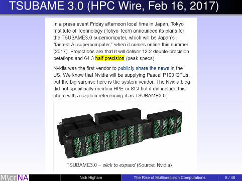
TSUBAME 3.0 (HPC Wire, Feb 16, 2017)


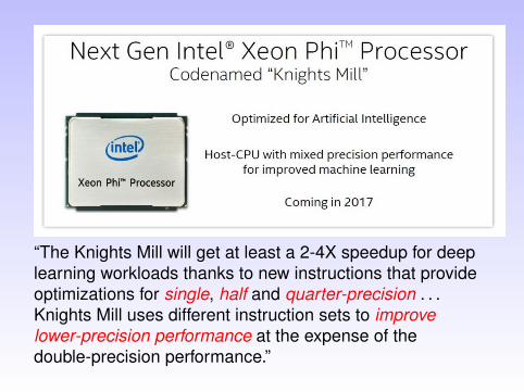
“The Knights Mill will get at least a 2-4X speedup for deeplearning workloads thanks to new instructions that provideoptimizations for single, half and quarter-precision . . .Knights Mill uses different instruction sets to improvelower-precision performance at the expense of thedouble-precision performance.”

“for machine learning as well as for certainimage processing and signal processingapplications, more data at lower precisionactually yields better results with certainalgorithms than a smaller amount of moreprecise data.”

Google Tensorflow Processor

“The TPU isspecial-purposehardware designed toaccelerate theinference phase in aneural network, in partthrough quantizing32-bit floating pointcomputations intolower-precision 8-bitarithmetic.”


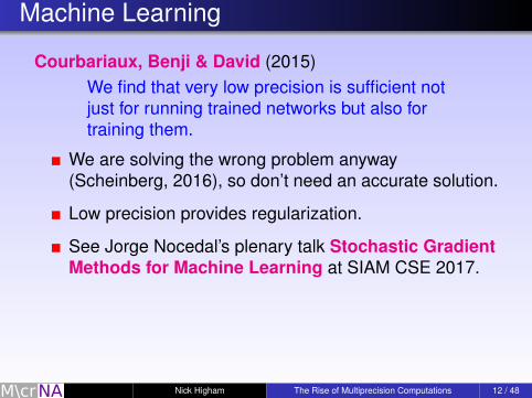
Machine Learning

Courbariaux, Benji & David (2015)We find that very low precision is sufficient notjust for running trained networks but also fortraining them.

We are solving the wrong problem anyway(Scheinberg, 2016), so don’t need an accurate solution.

Low precision provides regularization.

See Jorge Nocedal’s plenary talk Stochastic GradientMethods for Machine Learning at SIAM CSE 2017.


https://www.pathlms.com/siam/courses/4150/sections/5843/video_presentations/42686

https://www.pathlms.com/siam/courses/4150/sections/5843/video_presentations/42686

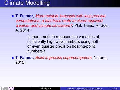
Climate Modelling

T. Palmer, More reliable forecasts with less precisecomputations: a fast-track route to cloud-resolvedweather and climate simulators?, Phil. Trans. R. Soc.A, 2014:

Is there merit in representing variables atsufficiently high wavenumbers using halfor even quarter precision floating-pointnumbers?

T. Palmer, Build imprecise supercomputers, Nature,2015.


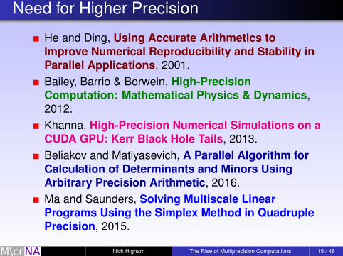
Need for Higher Precision

He and Ding, Using Accurate Arithmetics toImprove Numerical Reproducibility and Stability inParallel Applications, 2001.Bailey, Barrio & Borwein, High-PrecisionComputation: Mathematical Physics & Dynamics,2012.Khanna, High-Precision Numerical Simulations on aCUDA GPU: Kerr Black Hole Tails, 2013.Beliakov and Matiyasevich, A Parallel Algorithm forCalculation of Determinants and Minors UsingArbitrary Precision Arithmetic, 2016.Ma and Saunders, Solving Multiscale LinearPrograms Using the Simplex Method in QuadruplePrecision, 2015.


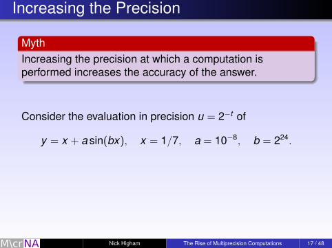
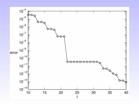
Increasing the Precision

MythIncreasing the precision at which a computation isperformed increases the accuracy of the answer.

Consider the evaluation in precision u = 2−t of

y = x + a sin(bx), x = 1/7, a = 10−8, b = 224.


10 15 20 25 30 35 4010

−14

10−13

10−12

10−11

10−10

10−9

10−8

10−7

10−6

10−5

10−4

t

error

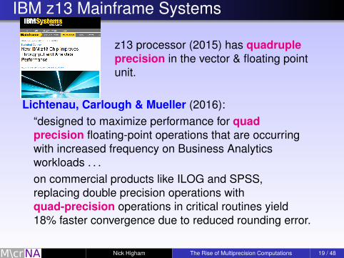
IBM z13 Mainframe Systems

z13 processor (2015) has quadrupleprecision in the vector & floating pointunit.

Lichtenau, Carlough & Mueller (2016):“designed to maximize performance for quadprecision floating-point operations that are occurringwith increased frequency on Business Analyticsworkloads . . .on commercial products like ILOG and SPSS,replacing double precision operations withquad-precision operations in critical routines yield18% faster convergence due to reduced rounding error.


Availability of Multiprecision in Software

Maple, Mathematica, PARI/GP, Sage.

MATLAB: Symbolic Math Toolbox, MultiprecisionComputing Toolbox (Advanpix).

Julia: BigFloat.

Mpmath and SymPy for Python.

GNU MP Library.

GNU MPFR Library.

(Quad only): some C, Fortran compilers.

Gone, but not forgotten:

Numerical Turing: Hull et al., 1985.


Note on Log Tables

Name Year Range Decimal placesR. de Prony 1801 1− 10,000 19

Edward Sang 1875 1− 20,000 28

Age 82

Edward Sang (1805–1890).Born in Kirkcaldy.Teacher of maths and actuary inEdinburgh.

It’s better to be approximately right thanprecisely wrong.


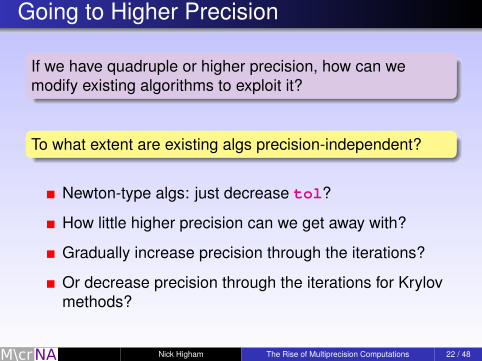
Going to Higher Precision

If we have quadruple or higher precision, how can wemodify existing algorithms to exploit it?

To what extent are existing algs precision-independent?

Newton-type algs: just decrease tol?

How little higher precision can we get away with?

Gradually increase precision through the iterations?

Or decrease precision through the iterations for Krylovmethods?


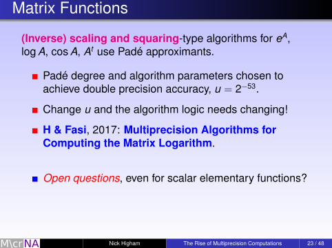
Matrix Functions

(Inverse) scaling and squaring-type algorithms for eA,log A, cos A, At use Padé approximants.

Padé degree and algorithm parameters chosen toachieve double precision accuracy, u = 2−53.

Change u and the algorithm logic needs changing!

H & Fasi, 2017: Multiprecision Algorithms forComputing the Matrix Logarithm.

Open questions, even for scalar elementary functions?


http://eprints.ma.man.ac.uk/2548/


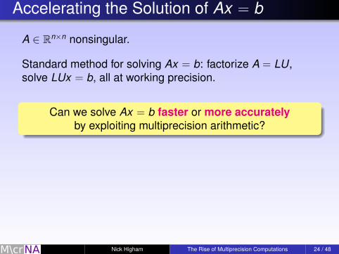
Accelerating the Solution of Ax = b

A ∈ Rn×n nonsingular.

Standard method for solving Ax = b: factorize A = LU,solve LUx = b, all at working precision.

Can we solve Ax = b faster or more accuratelyby exploiting multiprecision arithmetic?


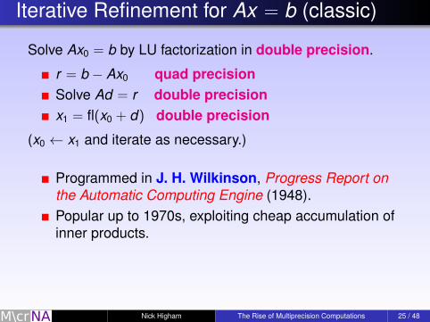
Iterative Refinement for Ax = b (classic)

Solve Ax0 = b by LU factorization in double precision.

r = b − Ax0 quad precisionSolve Ad = r double precisionx1 = fl(x0 + d) double precision

(x0 ← x1 and iterate as necessary.)

Programmed in J. H. Wilkinson, Progress Report onthe Automatic Computing Engine (1948).Popular up to 1970s, exploiting cheap accumulation ofinner products.


Iterative Refinement (1970s, 1980s)

Solve Ax0 = b by LU factorization.r = b − Ax0

Solve Ad = rx1 = fl(x0 + d)

Everything in double precision.

Skeel (1980).Jankowski & Wozniakowski (1977) for a general solver.


Iterative Refinement (2000s)

Solve Ax0 = b by LU factorization in single precision.

r = b − Ax0 double precisionSolve Ad = r single precisionx1 = fl(x0 + d) double precision

Dongarra, Langou et al. (2006).Motivated by single precision being at least twice asfast as double.


Iterative Refinement in Three PrecisionsJoint work with Erin Carson (NYU).

A,b given in precision u.Solve Ax0 = b by LU factorization in precision uf .

r = b − Ax0 precision ur

Solve Ad = r precision uf

x1 = fl(x0 + d) precision u

Three previous usages are special cases.Choose precisions from half, single, double, quadruplesubject to ur ≤ u ≤ uf .Can we compute more accurate solutions faster?


http://math.nyu.edu/~erinc/

Existing Rounding Error Analysis

Wilkinson (1963): fixed-point arithmetic.Moler (1967): floating-point arithmetic.Higham (1997, 2002): more general analysis forarbitrary solver.Langou et al. (2006): lower precision LU.

All the above require support at most two precisions andrequire κ(A)u < 1 .


New Analysis

Assume computed solution to Adi = ri satisfies

‖di − di‖∞‖di‖

≤ uf θi < 1.

Define µi by

‖A(x − xi)‖∞ = µi‖A‖∞‖x − xi‖∞,

and note that

κ∞(A)−1 ≤ µi ≤ 1.


Condition Numbers

|A| = (|aij |).

cond(A, x) =‖ |A−1||A||x | ‖∞

‖x‖∞,

cond(A) = cond(A,e) = ‖ |A−1||A| ‖∞,

κ∞(A) = ‖A‖∞‖A−1‖∞.

1 ≤ cond(A, x) ≤ cond(A) ≤ κ∞(A).


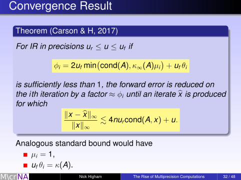
Convergence Result

Theorem (Carson & H, 2017)

For IR in precisions ur ≤ u ≤ uf if

φi = 2uf min(cond(A), κ∞(A)µi

)+ uf θi

is sufficiently less than 1, the forward error is reduced onthe ith iteration by a factor ≈ φi until an iterate x is producedfor which

‖x − x‖∞‖x‖∞

. 4nur cond(A, x) + u.

Analogous standard bound would haveµi = 1,uf θi = κ(A).


Precision Combinations

H = half, S = single, D = double, Q = quad. “uf u ur ”:

Traditional:

SSDDDQHHSHHDHHQSSQ

1970s/1980s:

SSSDDDHHHQQQ

2000s:

SDDHSSDQQHDDHQQSQQ

3 precisions:

HSDHSQHDQSDQ


Results (1)

Backward erroruf u ur κ∞(A) norm comp Forward errorH S S 104 S S cond(A, x) · SH S D 104 S S SH D D 104 D D cond(A, x) · DH D Q 104 D D DS S S 108 S S cond(A, x) · SS S D 108 S S SS D D 108 D D cond(A, x) · DS D Q 108 D D D


Results (2): HSD vs. SSD

Backward erroruf u ur κ∞(A) norm comp Forward errorH S S 104 S S cond(A, x) · SH S D 104 S S SH D D 104 D D cond(A, x) · DH D Q 104 D D DS S S 108 S S cond(A, x) · SS S D 108 S S SS D D 108 D D cond(A, x) · DS D Q 108 D D D

Can we get the benefit of “HSD” while allowing a largerrange of κ∞(A)?


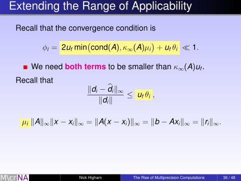
Extending the Range of Applicability

Recall that the convergence condition is

φi = 2uf min(cond(A), κ∞(A)µi

)+ uf θi � 1.

We need both terms to be smaller than κ∞(A)uf .

Recall that‖di − di‖∞‖di‖

≤ uf θi ,

µi ‖A‖∞‖x − xi‖∞ = ‖A(x − xi)‖∞ = ‖b − Axi‖∞ = ‖ri‖∞.


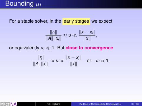
Bounding µi

For a stable solver, in the early stages we expect

‖ri‖‖A‖‖xi‖

≈ u � ‖x − xi‖‖x‖

,

or equivalently µi � 1. But close to convergence

‖ri‖‖A‖‖xi‖

≈ u ≈ ‖x − xi‖‖x‖

or µi ≈ 1.


Bounding θi

uf θi bounds rel error in solution of Adi = ri .We need uf θi � 1.

Standard solvers cannot achieve this for very ill conditioned A!

Empirically observed by Rump (1990) that if L and U arecomputed LU factors of A from GEPP then

κ(L−1AU−1) ≈ 1 + κ(A)u,

even for κ(A)� u−1.


Preconditioned GMRES

To compute the updates di we apply GMRES to

U−1L−1A︸︷︷︸A

di = U−1L−1ri .

A is applied in twice the working precision.

κ(A)� κ(A) typically.

Rounding error analysis shows we get an accurate di

even for numerically singular A.Call the overall alg GMRES-IR.


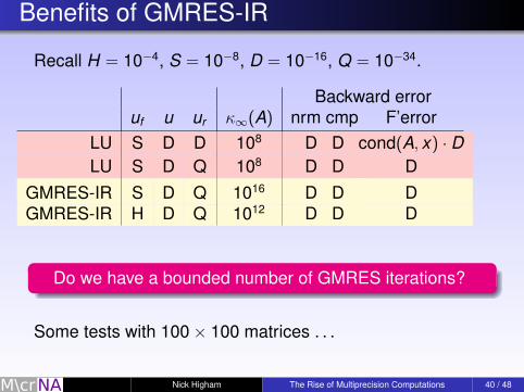
Benefits of GMRES-IR

Recall H = 10−4, S = 10−8, D = 10−16, Q = 10−34.

Backward erroruf u ur κ∞(A) nrm cmp F’error

LU S D D 108 D D cond(A, x) · DLU S D Q 108 D D D

GMRES-IR S D Q 1016 D D DGMRES-IR H D Q 1012 D D D

Do we have a bounded number of GMRES iterations?

Some tests with 100× 100 matrices . . .


Test 1: LU-IR, (uf ,u,ur) = (S,D,D)

κ∞(A) ≈ 1010, σi = αi Divergence

0 1 2

re-nement step

10-15

10-10

10-5

100 ferrnbecbe


Test 1: LU-IR, (uf ,u,ur) = (S,D,Q)

κ∞(A) ≈ 1010, σi = αi Divergence

0 1 2

re-nement step

10-15

10-10

10-5

100 ferrnbecbe


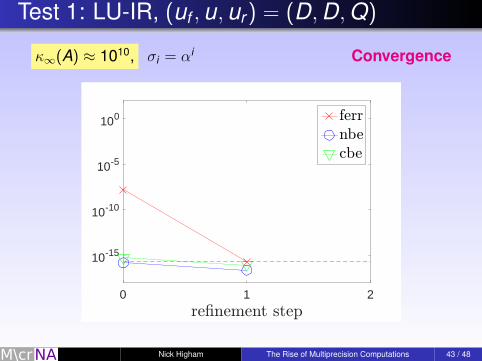
Test 1: LU-IR, (uf ,u,ur) = (D,D,Q)

κ∞(A) ≈ 1010, σi = αi Convergence

0 1 2

re-nement step

10-15

10-10

10-5

100 ferrnbecbe


Test 1: GMRES-IR, (uf ,u,ur) = (S,D,Q)

κ∞(A) ≈ 1010, σi = αi , GMRES its (2,3) Convergence

0 1 2

re-nement step

10-15

10-10

10-5

100 ferrnbecbe


Test 2: GMRES-IR, (uf ,u,ur) = (H,D,Q)

κ∞(A) ≈ 102, 1 small σi , GMRES its (8,8,8) Convergence

0 1 2 3

re-nement step

10-15

10-10

10-5

100 ferrnbecbe


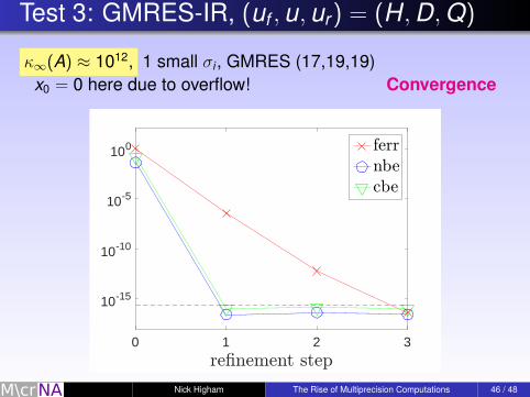
Test 3: GMRES-IR, (uf ,u,ur) = (H,D,Q)

κ∞(A) ≈ 1012, 1 small σi , GMRES (17,19,19)x0 = 0 here due to overflow! Convergence

0 1 2 3

re-nement step

10-15

10-10

10-5

100 ferrnbecbe


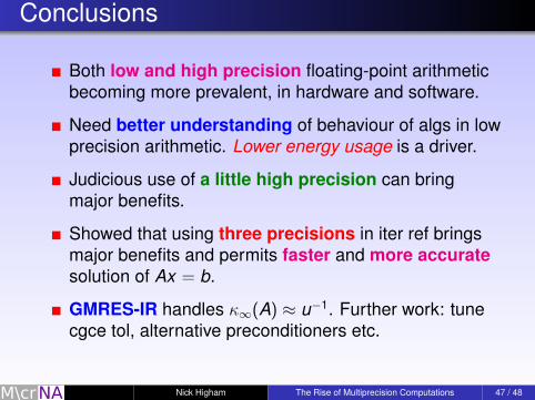
Conclusions

Both low and high precision floating-point arithmeticbecoming more prevalent, in hardware and software.

Need better understanding of behaviour of algs in lowprecision arithmetic. Lower energy usage is a driver.

Judicious use of a little high precision can bringmajor benefits.

Showed that using three precisions in iter ref bringsmajor benefits and permits faster and more accuratesolution of Ax = b.

GMRES-IR handles κ∞(A) ≈ u−1. Further work: tunecgce tol, alternative preconditioners etc.


Erin Carson and & H (2017), A New Analysis of IterativeRefinement and its Application to Accurate Solution ofIll-Conditioned Sparse Linear Systems, MIMS EPrint2017.12, The University of Manchester, March 2017; underrevision for SIAM J. Sci. Comput.

Erin Carson and & H (2017), Accelerating the Solution ofLinear Systems by Iterative Refinement in ThreePrecisions, MIMS EPrint 2017.24, The University ofManchester, July 2017.





http://eprints.ma.man.ac.uk/2562



References I

D. H. Bailey, R. Barrio, and J. M. Borwein.High-precision computation: Mathematical physics anddynamics.Appl. Math. Comput., 218(20):10106–10121, 2012.

G. Beliakov and Y. Matiyasevich.A parallel algorithm for calculation of determinants andminors using arbitrary precision arithmetic.BIT, 56(1):33–50, 2015.


References II

E. Carson and N. J. Higham.A new analysis of iterative refinement and its applicationto accurate solution of ill-conditioned sparse linearsystems.MIMS EPrint 2017.12, Manchester Institute forMathematical Sciences, The University of Manchester,UK, Mar. 2017.23 pp.Revised July 2017. Submitted to SIAM J. Sci. Comput.

M. Courbariaux, Y. Bengio, and J.-P. David.Training deep neural networks with low precisionmultiplications, 2015.ArXiv preprint 1412.7024v5.


References III

A. D. D. Craik.The logarithmic tables of Edward Sang and hisdaughters.Historia Mathematica, 30(1):47–84, 2003.

Y. He and C. H. Q. Ding.Using accurate arithmetics to improve numericalreproducibility and stability in parallel applications.J. Supercomputing, 18(3):259–277, 2001.

N. J. Higham.Iterative refinement for linear systems and LAPACK.IMA J. Numer. Anal., 17(4):495–509, 1997.


References IV

N. J. Higham.Accuracy and Stability of Numerical Algorithms.Society for Industrial and Applied Mathematics,Philadelphia, PA, USA, second edition, 2002.ISBN 0-89871-521-0.xxx+680 pp.

G. Khanna.High-precision numerical simulations on a CUDA GPU:Kerr black hole tails.J. Sci. Comput., 56(2):366–380, 2013.


References V

J. Langou, J. Langou, P. Luszczek, J. Kurzak, A. Buttari,and J. Dongarra.Exploiting the performance of 32 bit floating pointarithmetic in obtaining 64 bit accuracy (revisitingiterative refinement for linear systems).In Proceedings of the 2006 ACM/IEEE Conference onSupercomputing, Nov. 2006.

C. Lichtenau, S. Carlough, and S. M. Mueller.Quad precision floating point on the IBM z13.In 2016 IEEE 23nd Symposium on Computer Arithmetic(ARITH), pages 87–94, July 2016.


References VI

D. Ma and M. Saunders.Solving multiscale linear programs using the simplexmethod in quadruple precision.In M. Al-Baali, L. Grandinetti, and A. Purnama, editors,Numerical Analysis and Optimization, number 134 inSpringer Proceedings in Mathematics and Statistics,pages 223–235. Springer-Verlag, Berlin, 2015.

K. Scheinberg.Evolution of randomness in optimization methods forsupervised machine learning.SIAG/OPT Views and News, 24(1):1–8, 2016.


The Rise of Multiprecision Computationshigham/talks/arith17.pdf · Research Matters February 25,...

Documents

Transcript of The Rise of Multiprecision Computationshigham/talks/arith17.pdf · Research Matters February 25,...