The Rise of Market Powerand the Macroeconomic Implications∗

Jan De Loecker†KU Leuven and Princeton University

NBER and CEPR

Jan Eeckhout‡UPF-ICREA-GSE and UCL

August 24, 2017

Abstract

We document the evolution of markups based on firm-level data for the US economysince 1950. Initially, markups are stable, even slightly decreasing. In 1980, average markupsstart to rise from 18% above marginal cost to 67% now. There is no strong pattern acrossindustries, though markups tend to be higher, across all sectors of the economy, in smallerfirms and most of the increase is due to an increase within industry. We do see a notablechange in the distribution of markups with the increase exclusively due to a sharp increasein high markup firms.We then evaluate the macroeconomic implications of an increase in average market power,which can account for a number of secular trends in the last 3 decades: 1. decrease in laborshare; 2. decrease in capital share; 3. decrease in low skill wages; 4. decrease in labor forceparticipation; 5. decrease in labor flows; 6. decrease in migration rates; 7. slowdown inaggregate output.

Keywords: Markups; Market Power; Secular Trends; Labor Market.

JEL: E2, D2, D4, J3, K2, L1

∗We would like to thank Mark Aguiar, Pol Antras, John Asker, Eric Bartelsman, Steve Berry, Emmanuel Farhi,Bob Hall, John Haltiwanger, Xavier Gabaix, Eric Hurst, Loukas Karabarbounis, Patrick Kehoe, Pete Klenow, EstebanRossi-Hansberg, Chad Syverson, Jo Van Biesebroeck and Frank Verboven for insightful discussions and comments.Shubhdeep Deb, Morgane Guignard and David Puig provided invaluable research assistance. De Loecker gratefullyacknowledges support from the FWO Odysseus Grant and Eeckhout from the ERC, Advanced grant 339186, andfrom ECO2015-67655-P.†jan.deloecker@kuleuven.be.‡j.eeckhout@ucl.ac.uk.

1

1 Introduction

The macroeconomy is experiencing a fundamental long term change in the last decades at alower frequency than the business cycle. This manifests itself in a number of secular trends:some are related to labor market outcomes such as a declining labor share, declining wagesand declining labor force participation; others to the slowdown in labor market dynamism withdecreased job mobility and lower migration rates; and yet others are related to the capital shareand the growth of output. While many explanations have been proposed for each of thesesecular trends, in this paper we argue that all these trends are consistent with one commoncause that hitherto has remained undocumented, the rise in market power since 1980.1

The presence of market power has implications for welfare and resource allocation. Firmsthat can command a price above marginal cost produce less output. In addition to loweringconsumer welfare, this has implications for factor demand, for the distribution of economicrents, and for business dynamics such as entry and exit, and resource allocation. In this paperwe aim to achieve two goals. First, we document the evolution of markups for the US economysince 1950. Based on firm-level data, we find that while market power was more or less constantbetween 1950 and 1980, there has been a steady rise in market power since 1980, from 18%above cost to 67% above cost. Over a 35 year period, that is an increase in the price levelrelative to cost of 1% per year. Second, we investigate the macroeconomic implications of thisrise in market power and the general equilibrium effects it has. We show that the rise in marketpower is consistent with seven secular trends in the last three decades.

While there is ample evidence that market power exists for particular markets and that it ispervasive across sectors, there is surprisingly little systematic evidence of the patterns of mar-ket power across the aggregate economy, and over time. The evidence on market power wedo have comes from case studies of specific industries for which researchers have access to de-tailed data and for which they can estimate markups as a proxy for market power. The estima-tion of markups traditionally relies on assumptions on consumer behavior coupled with profitmaximization, and an imposed model of how firms compete, e.g., Bertrand-Nash in prices.

The fundamental challenge that this approach confronts is the notion that marginal costsof production are fundamentally not observed, requiring more structure to uncover it from thedata. Optimal pricing therefore relates observed price data to estimates of substitution elas-ticities to uncover the marginal cost of production, and consequently the markup. The com-bination of requiring data on consumer demand (containing prices, quantities, characteristics,consumer attributes, etc.) and the need for specifying a model of conduct, have limited the useof the so-called demand approach to particular markets.

In this paper we follow a radically different approach to estimate markups, following re-cent advances in the literature on markup estimation by De Loecker and Warzynski (2012) thatbuilds on Hall (1988), the so-called production-approach. This approach relies on individualfirm output and input data, covering a panel of producers over time, and in contrast to the

1Outside of the academic literature it has received significant attention, e.g. A lapse in concentration (TheEconomist, September 2016), and the CEA Issue Brief, Benefits of Competition and Indicators of Market Power(May 2016).

2

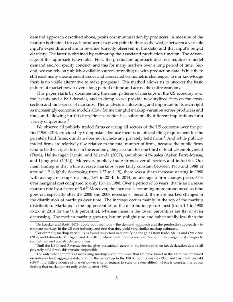
demand approach described above, posits cost minimization by producers. A measure of themarkup is obtained for each producer at a given point in time as the wedge between a variableinput’s expenditure share in revenue (directly observed in the data) and that input’s outputelasticity. The latter is obtained by estimating the associated production function. The advan-tage of this approach is twofold. First, the production approach does not require to modeldemand and/or specify conduct, and this for many markets over a long period of time. Sec-ond, we can rely on publicly available sources providing us with production data. While therestill exist many measurement issues and associated econometric challenges, to our knowledgethere is no viable alternative to make progress.2 This method allows us to uncover the basicpattern of market power over a long period of time and across the entire economy.

This paper starts by documenting the main patterns of markups in the US economy overthe last six and a half decades, and in doing so we provide new stylized facts on the cross-section and time-series of markups. This analysis is interesting and important in its own rightas increasingly economic models allow for meaningful markup variation across producers andtime; and allowing for this firm/time variation has substantially different implications for avariety of questions.3

We observe all publicly traded firms covering all sectors of the US economy over the pe-riod 1950-2014, provided by Compustat. Because there is no official filing requirement for theprivately held firms, our data does not include any privately held firms.4 And while publiclytraded firms are relatively few relative to the total number of firms, because the public firmstend to be the largest firms in the economy, they account for one third of total US employment(Davis, Haltiwanger, Jarmin, and Miranda (2007)) and about 41% sales (Asker, Farre-Mensa,and Ljungqvist (2014)). Moreover, publicly trade firms cover all sectors and industries Ourmain finding is that while average markups were fairly constant between 1960 and 1980 ataround 1.2 (slightly decreasing from 1.27 to 1.18), there was a sharp increase starting in 1980with average markups reaching 1.67 in 2014. In 2014, on average a firm charges prices 67%over marginal cost compared to only 18% in 1980. Over a period of 35 years, that is an increasemarkup rate by a factor of 3.6.5 Moreover, the increase is becoming more pronounced as timegoes on, especially after the 2000 and 2008 recessions. Second, there are marked changes inthe distribution of markups over time. The increase occurs mainly in the top of the markupdistribution. Markups in the top percentiles of the distribution go up most (from 1.4 in 1980to 2.6 in 2014 for the 90th percentile), whereas those in the lower percentiles are flat or evendecreasing. The median markup goes up, but only slightly so and substantially less than the

2De Loecker and Scott (2016) apply both methods – the demand approach and the production approach – toestimate markups in the US beer industry, and find that they yield very similar markup estimates.

3For example, markup variability is found important in quantifying the gains from trade, Melitz and Ottaviano(2008) and Edmonds, Midrigan, and Xu (2015), where trade reforms are best thought of as (exogenous) changes tocompetition and cost structures of firms.

4Until the US Inland Revenue Service gives researchers access to the information on tax declaration data of allprivately held firms, this remains impossible.

5The only other attempts at measuring markups economy-wide that we have found in the literature are basedon industry level aggregate data, and for the period up to the 1980s. Both Burnside (1996) and Basu and Fernald(1997) find little evidence of market power (nor of returns to scale or externalities), which is consistent with ourfinding that market power only picks up after 1980.

3

average markup. Third, there is no strong compositional pattern across industries and the in-crease occurs mainly within industry. Finally, across industries it is mainly the smaller firmsthat have higher markups, though this effect disappears at a narrow industry specification,indicating that there is systematic size differences across industries. Within narrowly-defined(here 4 digit) industries firm size and markups are positively correlated.

After we establish these main facts, we take these as given and we discuss the implicationsof the rise in market power for recent debates in the macro/labor literature. We take the risein markups as given, and we do not engage in the analysis of how this happened, which liesbeyond the scope of this paper, though we provide the reader with a few promising candidatesin the concluding remarks. In particular, we show how the rise in markups naturally gives riseto a decrease in the labor share, a decrease in the capital share, a decrease in low skilled wages,a decrease in labor market participation, and decrease in job flows, a decrease in interstatemigration, and finally, we show that properly accounting for the rise in markups, there is noproductivity slowdown but instead an increase in productivity despite the fact that outputgrowth has slowed down.

At a general level, our findings warrant a more systematic analysis of the aggregate impact,if any, of market power on a variety of outcomes of interest. While there was a tradition to in-vestigate the potential impact of market power on resource allocation, the analysis of Harberger(1954) concluded that profit rates across US (manufacturing) industries during the 1920s werenot sufficiently dispersed to generate any meaningful aggregate outcome. This analysis, andits conclusion that market power barely impacts economy-wide outcomes, became the defaultview held by many economists and policy makers ever since.6

The paper is organized as follows. In Section 2 the data and empirical framework to re-cover markups is presented. The main facts on markups, in both the cross-section and the timeseries, are presented in Section 3. We derive the macroeconomic implication in Section 4, tak-ing the facts from the previous section as given, building on a stylized model of market-levelcompetition and an aggregate labor market. We conclude in Section 5.

2 Empirical Framework

In this section we discuss the empirical framework and the main data source we rely on to de-scribe the patterns of markups in the US economy. In particular, we observe firm-level outputand input data for firms across the US economy. This data is sufficient to measure firm-levelmarkups using minimal assumptions on producer behavior, but without assumptions on prod-uct market competition and consumer demand. We apply the method proposed by De Loeckerand Warzynski (2012), and we discuss the implementation.

6See Asker, Collard-Wexler, and De Loecker (2017) for a discussion, and an application to the oil industry.

4

2.1 Data

The choice of data is driven entirely by the ability to cover the longest possible period of time,and to have a wide coverage of economic activity. This for example rules out using the censusof manufacturing establishments, given the decreasing share of manufacturing in the overallemployment of US economy, from about 25% in 1960 to 9% in 2014 (Baily and Bosworth (2014)).To our knowledge, Compustat is the only data source that provides substantial coverage offirms in the private sector over a substantial period of time, covering the period 1950 to 2014.While publicly traded firms are relatively few relative to the total number of firms, because thepublic firms tend to be the largest firms in the economy, they account for one third of total USemployment (Davis, Haltiwanger, Jarmin, and Miranda (2007)) and about 41% sales (Asker,Farre-Mensa, and Ljungqvist (2014)).

There are two alternatives to using our publicly trade firms data. A first alternative datasource is the Census of Manufacturing, but it accounts for only 8.8% of US employment in 2013.Moreover, the Census of Manufacturing is – by construction – highly selective in the sectorsand industries covered. We establish in Appendix B.1 that for manufacturing only, the sameresult holds. A second alternative data source is to use aggregate industry-level data ratherthan micro-level data, as originally done by Hall (1988). We perform this robustness analysisin Appendix B.4 both on aggregate IRS data and an aggregation of our own data of publicfirms. The aggregate patterns across the (aggregate) Compustat dataset and the economy-wideprivate sector (using IRS) are very similar.

The Compustat data contains firm-level balance sheet information, which allows us to relyon the so-called production approach to measuring markups, and market power. In particularwe observe measures of sales, input expenditure, capital stock information, as well as detailedindustry activity classifications.7 In addition, we observe relevant, and direct accounting in-formation of profitability and stock market performance. The latter information is useful toverify whether our measures of markups, as discussed below, are at all correlated to the overallevaluation of the market. Table A.1 in the Appendix provides basic summary statistics of thefirm-level panel data used throughout the empirical analysis.

2.2 Markup estimation

Measuring markups is notoriously hard as marginal cost data is not readily available, let aloneprices, for a large representative sample of firms. The standard approach in modern Indus-trial Organization is to specify a particular demand system that delivers price-elasticities ofdemand, which combined with assumptions on how firms compete, in turn deliver measuresof markups through the first order condition associated with optimal pricing. This approach,while powerful in other settings, is not useful here for two distinct reasons. First, we do notwant to impose a specific model of how firms compete across a dataset of large firms, or com-

7The Compustat data has been used extensively in the literature related to issues of corporate finance, such asCEO pay, e.g. Gabaix and Landier (2008), but also for questions of productivity and multinational ownership, e.g.Keller and Yeaple (2009).

5

mit to a particular demand system for all the products under consideration. Second, even ifwe wanted to make all these assumptions, there is simply no information on prices and quan-tities at the product level for a large set of sectors of the economy, over a long period of time,to successfully estimate price elasticities of demand, and specify particular models of pricecompetition for all sectors.

We rely on a recently proposed framework by De Loecker and Warzynski (2012), based onthe insight of Hall (1988) to estimate (firm-level) markups using standard balance sheet dataon firms, which does not require to make assumptions on demand and how firms compete. In-stead markups are obtained by leveraging cost minimization of a variable input of production.This approach requires an explicit treatment of the production function.

2.2.1 Producer behavior

Consider an economy with N firms, indexed by i = 1, ..., N . Firms are heterogeneous in theirproductivity and otherwise have access to a common production technology. In each period t,firm i minimizes the contemporaneous cost of production given the production function thattransforms inputs into the quantity of output Qit produced by the technology Q(·):

Q(Ωit,Vit,Kit) = ΩitFt(Vit,Kit), (1)

where V = (V 1, ..., V J) captures the set of variable inputs of production (including labor, inter-mediate inputs, materials,...), Kit is the capital stock and Ωit is the Hicks-neutral productivityterm that is firm-specific. Because in the implementation we will use information on a bundleof variable inputs, and not the individual inputs, in the exposition we treat the vector V as ascalar V . Following De Loecker and Warzynski (2012) we consider the associated Lagrangianobjective function:

L(Vit,Kit,Λit) = P Vit Vit + ritKit − Λit(Q(·)−Qit), (2)

where P V is the price of the variable input, r is the user cost of capital,8 Q(·) is the technology(1), Qit is a scalar and Λit is the Lagrangian multiplier. We consider the first order conditionwith respect to the variable input V , and this is given by:

∂Lit∂Vit

= P Vit − Λit∂Q(·)∂Vit

= 0. (3)

Multiplying all terms by Vit/Qit, and rearranging terms yields an expression of the outputelasticity of input V :

θVit ≡∂Q(·)∂Vit

VitQit

=1

Λit

P Vit VitQit

. (4)

8For our purpose here, we maintain the assumption that input markets are competitive and hence PV and r areequal to marginal revenue product. If they were not, then this will affect the marginal cost and hence the estimateof the markup. The are two opposing effects of market power in the inputs market: 1. Double marginalization, bywhich the marginal cost of inputs would be higher than under competition; 2. Monopsony power, where the firmssqueezes the upstream provider and obtains lower input prices. The measured markup will be biased but it is notclear in which direction. For an analysis with non-competitive inputs, see De Loecker, Goldberg, Khandelwal, andPavcnik (2016).

6

The Lagrangian parameter Λ is a direct measure of marginal cost – i.e. it is the value of theobjective function as we relax the output constraints. We define the markup as µ = P

Λ , whereP is the price for the output good, which depends on the extent of market power. We returnto that below. Substituting marginal cost for the markup to price ratio, we obtain a simpleexpression for the markup:

µit = θVitPitQit

P Vj

it Vit. (5)

The expression of the markup is derived without specifying conduct and/or a particular de-mand system. Note that with this approach to markup estimation, there are in principle mul-tiple first order conditions (of each variable input in production) that yield an expression forthe markup. Regardless of which variable input of production is used, there are two key ingre-

dients needed in order to measure the markup: the revenue share of the variable input, PVit VitPitQit

,and the output elasticity of the variable input, θVit . While this approach does not restrict theoutput elasticity, when implementing this procedure it depends on a specific production func-tion, and assumptions of underlying producer behavior in order to consistently estimate thiselasticity in the data. We turn to the implementation next.

2.2.2 Implementation

We directly observe sales, Sit = PitQit and total variable cost of production, Cit =∑

j PV jit V

jit ,

measured by the cost of goods sold. The Compustat data does not directly report a breakdownof the expenditure on variable inputs, such as labor, intermediate inputs, electricity, and others,and therefore we prefer to rely on the reported total variable cost of production.9

In order to recover markups an estimate of the output elasticity of this input bundle is re-quired. We follow standard practice and rely on a panel of firms, for which we estimate produc-tion functions by industry. In particular we consider various specifications of the productionfunction, both at the level of the economy and the industry. For the main results we considerindustry-specific Cobb-Douglas production functions, with variable inputs and capital.10

For a given industry we consider the production function:

qit = βvvit + βkkit + ωit + εit, (6)

where lower cases denote logs and ωit = ln Ωit, and where qit is measured as the log of deflatedfirm level sales.11 We follow the literature and control for the simultaneity and selection bias,inherently present in the estimation of the above equation, and rely on a control function ap-proach, paired with an AR(1) process for productivity to estimate the output elasticity of the

9We verify the robustness of our main findings to obtaining markup estimates using intermediate inputs only asthe variable input. The latter, however, requires additional assumptions on how to derive a measure of intermediateinput use from operating income before depreciations, and the total wage bill, where the latter is imputed frommultiplying the reported total number of employees with industry-wide wage data, as done in e.g. Keller andYeaple (2009).

10We also consider more flexible translog production functions, and Cobb-Douglas production functions withtime-varying coefficients. Appendix B discusses the main findings using these alternative specifications.

11See De Loecker and Warzynski (2012) for a discussion of the measurement of sales and quantities.

7

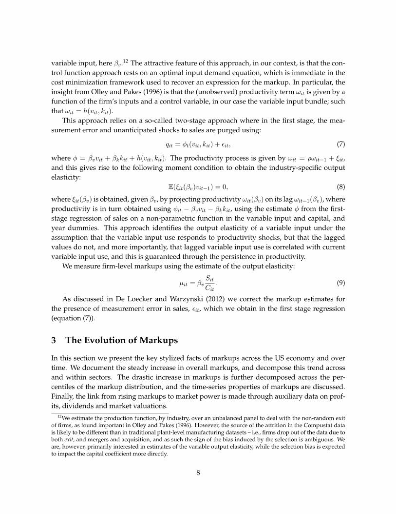
variable input, here βv.12 The attractive feature of this approach, in our context, is that the con-trol function approach rests on an optimal input demand equation, which is immediate in thecost minimization framework used to recover an expression for the markup. In particular, theinsight from Olley and Pakes (1996) is that the (unobserved) productivity term ωit is given by afunction of the firm’s inputs and a control variable, in our case the variable input bundle; suchthat ωit = h(vit, kit).

This approach relies on a so-called two-stage approach where in the first stage, the mea-surement error and unanticipated shocks to sales are purged using:

qit = φt(vit, kit) + εit, (7)

where φ = βvvit + βkkit + h(vit, kit). The productivity process is given by ωit = ρωit−1 + ξit,and this gives rise to the following moment condition to obtain the industry-specific outputelasticity:

E(ξit(βv)vit−1) = 0, (8)

where ξit(βv) is obtained, given βv, by projecting productivity ωit(βv) on its lag ωit−1(βv), whereproductivity is in turn obtained using φit − βvvit − βkkit, using the estimate φ from the first-stage regression of sales on a non-parametric function in the variable input and capital, andyear dummies. This approach identifies the output elasticity of a variable input under theassumption that the variable input use responds to productivity shocks, but that the laggedvalues do not, and more importantly, that lagged variable input use is correlated with currentvariable input use, and this is guaranteed through the persistence in productivity.

We measure firm-level markups using the estimate of the output elasticity:

µit = βvSitCit

. (9)

As discussed in De Loecker and Warzynski (2012) we correct the markup estimates forthe presence of measurement error in sales, εit, which we obtain in the first stage regression(equation (7)).

3 The Evolution of Markups

In this section we present the key stylized facts of markups across the US economy and overtime. We document the steady increase in overall markups, and decompose this trend acrossand within sectors. The drastic increase in markups is further decomposed across the per-centiles of the markup distribution, and the time-series properties of markups are discussed.Finally, the link from rising markups to market power is made through auxiliary data on prof-its, dividends and market valuations.

12We estimate the production function, by industry, over an unbalanced panel to deal with the non-random exitof firms, as found important in Olley and Pakes (1996). However, the source of the attrition in the Compustat datais likely to be different than in traditional plant-level manufacturing datasets – i.e., firms drop out of the data due toboth exit, and mergers and acquisition, and as such the sign of the bias induced by the selection is ambiguous. Weare, however, primarily interested in estimates of the variable output elasticity, while the selection bias is expectedto impact the capital coefficient more directly.

8

3.1 A Secular Trend since 1980

Figure 1 presents the weighted average markup, across the economy, over time where weightsare based on firm-level sales. Average markups have gone up since the 1980s. In the beginningof the sample period markups were stable and slightly decreasing from 1.27 in the 1960 to 1.18in 1980. Since 1980 there has been a steady increase to 1.67. In 2014, the average firm charges67% over marginal cost, compared to 18% in 1980. In Appendix B.5 we report some individualfirms’ markups.

1.1

1.2

1.3

1.4

1.5

1.6

1.7

Mar

kup

(Bas

elin

e)

1960 1970 1980 1990 2000 2010year

Figure 1: The Evolution of Average Markups (1960 - 2014). Average Markup is weighted bymarketshare of sales in the sample.

It is well known that the Compustat data is a selected sample and we therefore compareour result to aggregate data from the IRS, and further compare it to the aggregated version ofour data (Compustat). The figures in the Appendix B.4 confirm that these same pattern holds,at the aggregate level, although there is a more modest increase in market power for aggregatedata. The patterns, however, across the (aggregate) Compustat dataset and the economy-wideprivate sector (using IRS) are very similar. This highlights the importance of using micro-leveldata and that industry-level data cannot fully capture the increase in market power. We turnto the micro dimension next.

3.2 Decomposition: Markups and Firm Size

The construction of our measure of markup uses weights given by the sales share of the firmin the economy.13 When we compare our measure with the unweighted average of markup

13The pattern of aggregate markup depends on the aggregation weight used. The share of Sales is the most com-mon, see for example the HHI index. So far we made no assumption on demand and hence there is no welfaremeasure that guides us which aggregation weight to use. In the Appendix we report aggregate markups for alter-native aggregation weights employment and the value of variable inputs. We also report the joint distribution ofthe individual markup and the corresponding weight variable. The pattern of the increase in markups starting in

9

in Figure 2a, we observe that the unweighted average is even higher and also increasing morethan our benchmark measure: the unweighted markup goes from 1.4 in 1980 to 2.3 in 2014(and was fairly constant throughout the 1960s and 1970s), compared to an increase from 1.18to 1.67 for the unweighted measure. The fact that the unweighted measure is always higherindicates that larger firms (as measured by their sales) tend to have a lower markup. Thisappears at first to contradict the prediction from models of imperfect competition where firmswith larger market shares have higher markups. Of course, the previous results hold acrossall firms across all sectors, while within narrowly defined industries, however, we confirm thepositive relationship between markups and firm size.

1

1.5

2

2.5

1960 1970 1980 1990 2000 2010year

Share weighted Markup mu_mean

(a) Unweighted versus Weighted Markup.

1.2

1.3

1.4

1.5

1.6

1.7

1940 1960 1980 2000 2020year

Markup Mean 4digit

(b) Industry disaggregation

Figure 2: Decomposition by market share.

We seek to decompose the weighted mean to get at the source of this discrepancy in thelevel with the unweighted measure and to get at what has changed over time that can explainthe rise in markup. If in the total population, large firms have smaller markups, is this alsothe case at more disaggregated levels of industry? Is the change over time due to an overallincrease in markup (the markup tide has been lifting across all industries) or is there a changein the composition of firms of different sizes?

We therefore investigate whether this negative relation between markup and sales is due tothe composition of industry or due to the negative relation between size and markup, and usea decomposition method as in Olley and Pakes (1996).

THE CROSS-SECTIONAL DECOMPOSITION. Denote the share sit of firm i’s sales Sit = PitQit inthe total sales St in the economy (the universe of firms in our sample) by sit = Sit

St. Then we

can write the weighted markup, denoted by Mt, as

Mt =∑i

sitµit

= µt +∑i

(sit − st)(µit − µt) (10)

1980 is robust across the three weighting measures used: sales, employment and the value of variable inputs.

10

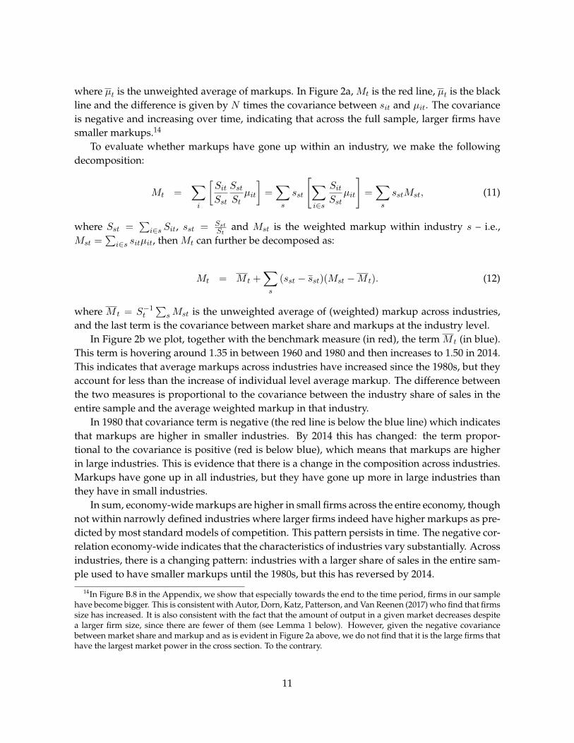
where µt is the unweighted average of markups. In Figure 2a, Mt is the red line, µt is the blackline and the difference is given by N times the covariance between sit and µit. The covarianceis negative and increasing over time, indicating that across the full sample, larger firms havesmaller markups.14

To evaluate whether markups have gone up within an industry, we make the followingdecomposition:

Mt =∑i

[SitSst

SstStµit

]=∑s

sst

[∑i∈s

SitSst

µit

]=∑s

sstMst, (11)

where Sst =∑

i∈s Sit, sst = SstSt

and Mst is the weighted markup within industry s – i.e.,Mst =

∑i∈s sitµit, then Mt can further be decomposed as:

Mt = M t +∑s

(sst − sst)(Mst −M t). (12)

where M t = S−1t

∑sMst is the unweighted average of (weighted) markup across industries,

and the last term is the covariance between market share and markups at the industry level.In Figure 2b we plot, together with the benchmark measure (in red), the term M t (in blue).

This term is hovering around 1.35 in between 1960 and 1980 and then increases to 1.50 in 2014.This indicates that average markups across industries have increased since the 1980s, but theyaccount for less than the increase of individual level average markup. The difference betweenthe two measures is proportional to the covariance between the industry share of sales in theentire sample and the average weighted markup in that industry.

In 1980 that covariance term is negative (the red line is below the blue line) which indicatesthat markups are higher in smaller industries. By 2014 this has changed: the term propor-tional to the covariance is positive (red is below blue), which means that markups are higherin large industries. This is evidence that there is a change in the composition across industries.Markups have gone up in all industries, but they have gone up more in large industries thanthey have in small industries.

In sum, economy-wide markups are higher in small firms across the entire economy, thoughnot within narrowly defined industries where larger firms indeed have higher markups as pre-dicted by most standard models of competition. This pattern persists in time. The negative cor-relation economy-wide indicates that the characteristics of industries vary substantially. Acrossindustries, there is a changing pattern: industries with a larger share of sales in the entire sam-ple used to have smaller markups until the 1980s, but this has reversed by 2014.

14In Figure B.8 in the Appendix, we show that especially towards the end to the time period, firms in our samplehave become bigger. This is consistent with Autor, Dorn, Katz, Patterson, and Van Reenen (2017) who find that firmssize has increased. It is also consistent with the fact that the amount of output in a given market decreases despitea larger firm size, since there are fewer of them (see Lemma 1 below). However, given the negative covariancebetween market share and markup and as is evident in Figure 2a above, we do not find that it is the large firms thathave the largest market power in the cross section. To the contrary.

11

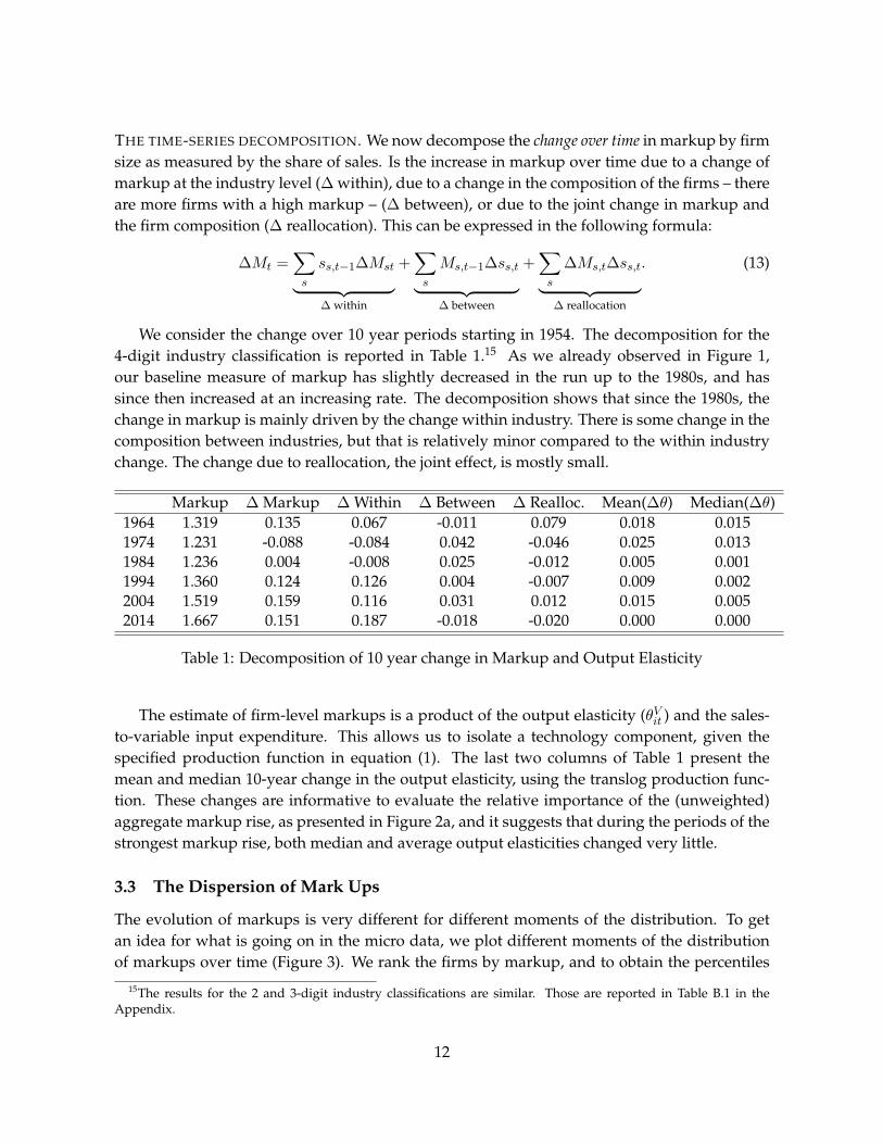
THE TIME-SERIES DECOMPOSITION. We now decompose the change over time in markup by firmsize as measured by the share of sales. Is the increase in markup over time due to a change ofmarkup at the industry level (∆ within), due to a change in the composition of the firms – thereare more firms with a high markup – (∆ between), or due to the joint change in markup andthe firm composition (∆ reallocation). This can be expressed in the following formula:

∆Mt =∑s

ss,t−1∆Mst︸ ︷︷ ︸∆ within

+∑s

Ms,t−1∆ss,t︸ ︷︷ ︸∆ between

+∑s

∆Ms,t∆ss,t︸ ︷︷ ︸∆ reallocation

. (13)

We consider the change over 10 year periods starting in 1954. The decomposition for the4-digit industry classification is reported in Table 1.15 As we already observed in Figure 1,our baseline measure of markup has slightly decreased in the run up to the 1980s, and hassince then increased at an increasing rate. The decomposition shows that since the 1980s, thechange in markup is mainly driven by the change within industry. There is some change in thecomposition between industries, but that is relatively minor compared to the within industrychange. The change due to reallocation, the joint effect, is mostly small.

Markup ∆ Markup ∆ Within ∆ Between ∆ Realloc. Mean(∆θ) Median(∆θ)1964 1.319 0.135 0.067 -0.011 0.079 0.018 0.0151974 1.231 -0.088 -0.084 0.042 -0.046 0.025 0.0131984 1.236 0.004 -0.008 0.025 -0.012 0.005 0.0011994 1.360 0.124 0.126 0.004 -0.007 0.009 0.0022004 1.519 0.159 0.116 0.031 0.012 0.015 0.0052014 1.667 0.151 0.187 -0.018 -0.020 0.000 0.000

Table 1: Decomposition of 10 year change in Markup and Output Elasticity

The estimate of firm-level markups is a product of the output elasticity (θVit ) and the sales-to-variable input expenditure. This allows us to isolate a technology component, given thespecified production function in equation (1). The last two columns of Table 1 present themean and median 10-year change in the output elasticity, using the translog production func-tion. These changes are informative to evaluate the relative importance of the (unweighted)aggregate markup rise, as presented in Figure 2a, and it suggests that during the periods of thestrongest markup rise, both median and average output elasticities changed very little.

3.3 The Dispersion of Mark Ups

The evolution of markups is very different for different moments of the distribution. To getan idea for what is going on in the micro data, we plot different moments of the distributionof markups over time (Figure 3). We rank the firms by markup, and to obtain the percentiles

15The results for the 2 and 3-digit industry classifications are similar. Those are reported in Table B.1 in theAppendix.

12

we weigh each firm by its market share. This makes the percentiles directly comparable to ourshare weighted average.

1

1.5

2

2.5

1960 1970 1980 1990 2000 2010year

Share weighted Markup p90 (ms) p50 (ms)p75 (ms)

Figure 3: The Evolution of the Distribution (Percentiles) of Markups (1950 - 2014). (The per-centiles of the Markup distribution are weighted by marketshare of sales in the sample.)

The increase in the average markup comes entirely from the firms with markups in the tophalf of the markup distribution. The median and lower percentiles are largely invariant overtime. For percentiles above the median, markups increase. Between 1980 and 2014, the 75thpercentile increases from 1.3 to 1.52, and the 90th percentile increases from 1.46 to 2.6.

3.4 The Process of Markups

Inspecting the time-series pattern of output, input and markup is directly relevant for studyingthe extent to which market power has changed over time. Figure 4 shows the evolution of thecross-sectional standard deviation of the shocks in the markup, sales and employment process,assuming this process is autoregressive:

xit = ρxit−1 + εit, x ∈ logµ, logS, logL. (14)

Starting in 1980, there is clearly a sharp rise in the standard deviation of the markup µ and amore moderate increase in that of sales S. Interestingly, there is much less of an increase in thestandard deviation of employment L. If anything, there is a decline from 2000 onwards. Theincrease in the standard deviation in markup is precisely driven by the increase in the wedgebetween the volatility of sales (increasing) and inputs, in this case labor (fairly constant andthen decreasing).16

This increasing wedge is consistent with the evidence in Decker, Haltiwanger, Jarmin, andMiranda (2014) that the shock process itself has not changed much but that the transmission

16We have also included higher order terms of the persistence and find that those are not important.

13

0

.2

.4

.6

.8

1950 1960 1970 1980 1990 2000 2010Data Year - Fiscal

Std(Markup) Std(Empl.) Std(Sales)

Figure 4: The Evolution of the Standard Deviation of Markups, Sales and Employment (1950 -2014). (AR(1) in logs on their lag with year and industry fixed effects )

of the shocks to inputs (labor) has. We revisit this lowering of the response of employmentto shocks in Section 4, and relate this to the fundamental change in pass-through of shocks tofactor demand, and output, consistent with an increase in overall market power.

3.5 Do Markups imply Market Power?

Markups tell us that the margin of revenue over variable costs has increased. That does notnecessarily imply that firms are making higher profits. If for example the source of the increasein markups is technological change that reduces variable costs, and the same technologicalchange increases the fixed costs. Consider for example high tech firms that produce softwareproducts that need one big up front investment and can be scaled nearly without any additionalcost. Such technological change will lead to higher markups (due to lower variable costs), butprices will not drop because firms need to generate revenue to cover fixed costs. As a result,profits will continue to be low and higher markups do not imply higher market power.

So the question is whether higher markups simultaneously lead to higher profits.17 In orderto address this issue, we need to have a measure of profits. Because the measure for profitsin Compustat is based on the cost of goods sold, this is not informative. The real value ofprofits corresponds to what firms pay their shareholders. For that we have two measures: 1.dividends and 2. the market value (or market capitalization). Dividends are the return aninvestor receives on holding equity in the firm. Of course, dividends may vary for reasons thathave nothing to do with the actual flow of profits. In particular, they will be closely related tothe investment opportunities that the firm has. Still, over a long enough horizon and averagingout over a large number of firms, we would expect that dividends are a good indicator of

17Profits do not necessarily derive exclusively from market power. There could be capital market imperfectionsthat constrain investment and lead to higher profits. However, in a model with both market power and financialfrictions, Cooper and Ejarque (2003) find that profitability is explained entirely by market power and none byfinancial frictions.

14

profits. The second measure, market value, is essentially the discounted sum of dividends,since a shareholder who sells shares in a firm gives up the opportunity value of receiving theindefinite stream of dividend payments. In contrast to the actual dividends, the market priceis not necessarily a good measure of contemporaneous profits since it takes into account allfuture dividends. In addition, it is highly susceptible to changes in expectations about futureprofitability of the firm. Nonetheless, in a cross section over a large number of firms, this shouldgive us some indication of the profitability of the firm.

Figure 5a clearly illustrates that the evolution of the weighted average of dividends closelytracks that of markups, with sharp reversal in the trend around 1980. The same is true formarket value (Figure 5b).

500000

1000000

1500000

2000000

Shar

e w

eigh

ted

Div

iden

d

1.1

1.2

1.3

1.4

1.5

1.6

1.7

Mar

kup

1960 1970 1980 1990 2000 2010year

Markup Share weighted Dividend

(a) Average Dividends (weighted)

0

2.00e+07

4.00e+07

6.00e+07

8.00e+07

Shar

e w

eigh

ted

Mar

ket V

alue

1.1

1.2

1.3

1.4

1.5

1.6

1.7

Mar

kup

1960 1970 1980 1990 2000 2010year

Markup Share weighted Market Value

(b) Average Market Value (weighted)

Figure 5: The Evolution of Average Dividends and Average Market Value (as a share of Sales)and Markup (1960 - 2014).

This is not just an artifact of the aggregate data. At the individual firm level, firms withhigher markups also have higher dividend margins. Figure B.7 in the Appendix shows thatrelation. For example, as the dividend margin increases from 0.2 to 0.7, the markup increasesfrom 2 to 3. This establishes that at the individual firm level, higher markups are not exclusivelydriven by technological change in a competitive market (basically higher fixed costs and/orlower variable costs). Higher markups result in higher dividends and therefore higher profits.

The variable profit rate (variable profits divided by sales) is directly related to the markupµ = P

c , where c is the marginal cost. This follows from the definition of the profit rate:

ΠV

PQ=

(P − c)QPQ

= 1− 1

µ, (15)

where we assume constant marginal costs and we do not subtract investment in capital. Thatis why this is a measure of variable profits.18 In an attempt to obtain external validation, wecompare the evolution of this measure of variable profits to the evolution of total profits. Wehave the data for the evolution of total profits for the economy as a whole from the national

18Of course, this is a poor measure of total profits since firms also have capital investment.

15

accounts data (which includes all firms, not just the publicly traded firms), depicted in Figure6, below.

.02

.04

.06

.08

.1.1

2

1950q1 1960q1 1970q1 1980q1 1990q1 2000q1 2010q1 2020q1time

Figure 6: Profit rates. Data from FRED, based on national accounts. Quarterly.

We compare the change in the variable profit rate using our measure of markup in equation(15) to the change in the aggregate profit rate. Since the national profit rate is calculated asa share of GDP and our measure is calculated as a share of total sales, we need to adjust ourmeasure for the variable profit rate for Gross National Income (GNI):

ΠV

GDP=

ΠV

PQ

GNI

GDP=

(1− 1

µ

)GNI

GDP. (16)

Using equation (16), and the fact that µ1980 = 1.18 and µ2014 = 1.67, we obtain an increase inthe profit share of GDP by a factor 2.34:19

ΠV2014GDP2014

ΠV1980GDP1980

= 2.34. (17)

The economy-wide profit rate relative to GDP, calculated from the national accounts, hasincreased fourfold between 1980 and 2014. This is an even bigger increase than the 2.34-foldincrease that we obtain from our markup measure. Of course, the two measures are not exactlycomparable. First, ours is a measure of variable profits and the national accounts measure isone of total profits which includes capital investments and fixed costs. This seems to indicatethat capital investment has increased less than variable costs. Second, the sample of firmsdiffers. Since ours is for publicly traded firms only, this may indicate that markups are evenhigher for those firms that are not publicly traded. The important conclusion is that there is anenormous increase in profits however it is measured, which is consistent with the increase inmarket power.

19This ratio of GNI/GDP is set at 0.502 in 1980 and 0.565 in 2014, as reported in the national accounts.

16

4 Macroeconomic Implications

We analyze the macroeconomic implications of the rise in market power. We establish 7 im-plications that follow from the observed increase in market power. For some implications, thisinvolves further analyzing the data that we have used to calculate the markup, and for otherimplications we develop a simple static model of industry competition, to illustrate how mar-ket power can generate the observed outcomes. In particular we will abstract from some of theheterogeneity that we see in the data.

Of course, given the simplicity of the model and the absence of an estimation, we do notpretend to evaluate the quantitative importance of market power for these implications, nor dowe claim that market power is the only force that contributes to these outcomes. We simplytake the observed markup trajectory as given and provide a simple framework to interpret var-ious aggregate labor and product market outcomes, without invoking any causal link betweenmarket power and the outcomes of interest. The latter lies beyond the scope of the currentpaper.

Implication 1. The Secular Decline in the Labor Share

In the national accounts, the labor share of income measures the expenditure on labor (thewage bill) divided by the total income generated. While there are business cycle fluctuations,the labor share has been remarkably constant since the second world war up to the 1980s, ataround 62%. Since 1980, there has been a secular decline all the way down to 56% (Bureau ofLabor Statistics Headline measure).20 The decline since the 1980s occurs in the large majorityof industries and across countries (see Karabarbounis and Neiman (2014) and Gollin (2002)).

Economists have not found conclusive evidence for the mechanism behind the decline inthe labor share. There are several candidate explanations. Karabarbounis and Neiman (2014)hypothesize that the decrease in the relative price of investment goods, due to informationtechnology, can explain half of the decline.21 An alternative explanation is the composition ofmanufacturing and services. Manufacturing tends to use a higher labor share than services, soit seems natural that with a change in the composition of industry shifting from manufacturingto industry, the labor share will decrease. However, this transition does not coincide with thetiming of the decrease in the labor share. In fact, most of the transition of manufacturing toservices happened before the 1980s (between 1950 and 1987, the share of manufacturing inoutput dropped from over two thirds to less than half, while the share of services doubled,from 21 to 40%, and that transition has slowed down since 1987, see Armenter (2015)).

Koh, Santaeulalia-Llopis, and Zheng (2017) offer yet another (and appealing) explanation,which is based on the increasing importance of intangible capital and its incomplete measure-ment as part of capital in aggregate data. Firms now invest substantially more in intellectual

20There are issues of measurement. See Elsby, Hobijn, and Sahin (2013) on the role of how labor income of theself-employed is imputed. Even after adjusting for measurement issues, the labor share still exhibits a seculardecline.

21Antras (2004) finds evidence that the technology is not Cobb-Douglas, which when estimated under competi-tion, is consistent with what we observe when there is a change in the markup.

17

property products and this leads to a lower expenditure on labor.22 However, in their worldwith perfect competition, this measurement issue should not lead to an increase in the totalprofit share. As we have documented above, the fourfold increase in the total profit rate in-dicates that if intangibles play a role, it must allow firms to exert more market power, whichis the central thesis of our paper.23 Finally, Elsby, Hobijn, and Sahin (2013) find little supportfor capital-labor substitution, nor for the role of a decline in unionization. They do find somesupport for off-shoring labor-intensive work as a potential explanation.

In the context of our setup, the change in the markup has an immediate implication for thelabor share. While we have calculated the markup from all variable inputs, we could do so aswell for labor alone. Then rewriting the First Order Condition (5), we obtain that at the firmlevel, the labor share wL

PQ satisfieswL

PQ=θLµ, (18)

where θL is the output elasticity of labor. Profit maximization by individual firms impliesan inversely proportional change in the labor share. As markup increases and provided thetechnology parameter θ remains unchanged over time, we expect to see an decrease in thelabor share.

Unfortunately Compustat does not have good data for the wage bill.24 We can therefore notdirectly verify condition (18) at the firm level.25 Instead, we rely on aggregate data from the BLS.They report total compensation of employees (expenditure on wages and salaries) as a shareof gross domestic income. We compare this BLS measure to a population average of the righthand side of (18), where we assume that the technology parameter has remained unchanged.We use as a measure for markups the one that we calculated above based on total variable costs(COGS) and not the cost of labor because we have no reliable data on the wage bill. We plotthis in Figure 7 where we normalize these measures to 100 at the start of our data in 1950.

Our main finding is that the labor share (in green) tracks the inverse markup quite closely,especially since 1980. It seems that the labor share is decreasing somewhat more slowly thanthe inverse of the average markup, but overall the trend is similar. The fact that this aggre-gate measure of labor share tracks the inverse of markups is quite remarkable since we areimplicitly making the following assumptions, due to absence of good firm-level wage data. We

22Intangible assets are non-physical assets including patents, trademarks, copyrights, franchises,... that grantrights and privileges, and have value for the owner.

23 For valuation purposes, intangible assets are valued using different methods including the market approach(how much is another party willing to pay to obtain the rights to those assets), the income approach (the streamof income the assets generate) and the cost approach (how much it would cost to replace the existing asset). Ifthe company has laid out expenses in the past (labor, advertising, R&D,...) to generate the intangibles then they arealready measured either in the variable inputs or in the capital inputs. If Coca Cola has invested in building its brandor a pharmaceutical in a drug, then those expenditures are included in variable inputs or capital at some point. Ifthe current value of the brand or the drug is higher than that intangible, then the value assigned to intangiblesincludes the expected stream of future profits net of the invested capital. Intangibles are therefore an alternativemeasure of the discounted stream of profits.

24There is good data on employment (EMP) but the data on the average compensation (XLR) in the firm is heavilyunderreported.

25Although with additional assumptions on the structure of wages a firm level analysis is feasible.

18

70

80

90

100

110

1940 1960 1980 2000 2020Data Year - Fiscal

Share weighted (Inverse) Markup Labor Share (Fred)

Figure 7: The Evolution of the labor share (BLS), and inverse of the markup (1960-2014) Notes:Labor Share data from BLS. Share of gross domestic income: Compensation of employees, paid:Wages and salary accruals. Disbursements, to persons. 1950=100.

basically treat every worker to be identical in each firm since we only have one markup mea-sure per firm and our model assumes that labor adjusts only in the number workers, not in thecomposition. Moreover, the markup µi in each firm is calculated based on all variable inputs(labor L and material inputsM ), whereas the first order condition (18) is supposed to hold for amarkup calculated based on labor alone. The association between the declining labor share andthe rising (aggregate) market power is robust to the specific weights used to construct the ag-gregate markup index; Figure B.4 in the Appendix presents the share-weighted markup usingalternative weights.

Implication 2. The Secular Decline in the Capital Share

The same logic for the decline in the labor share also applies to materialsM , i.e. variable inputsthat are used in production. Those are included in our variable cost measure COGS. Now if weconsider the evolution of capital investment, which is not included our measure of variable costand which adjusts at a lower and more long run frequency, then in the increase in markup hasimplications for the capital share.26 While the decline in the labor share is widely discussed,the decline in the capital share has received much less attention.27

Using a simple accounting rule, we can write the firm’s sales as: PQ = P V V + rK + Π

where r is the user cost of fixed capital and Π is total profits. Even if capital does not adjust at

26This is independent of the frequency at which capital adjusts. Implicit in our assumptions is the fact thatvariable inputs, which consist of labor L and material inputs M , adjust at a frequency higher than one year, ourunit of time, and capital does not. This assumption allows us to calculate the markup.

27A notable exception is Barkai (2017). He uses aggregate data: value added and compensation from the NationalIncome and Productivity Accounts (NIPA), and capital from the Bureau of Economic Analysis Fixed Asset Table.Instead, we use firm-level data.

19

.6

.65

.7

.75

.8

.85

MAR

KUP_INV

.06

.08

.1

.12

.14

.16

k_share_agg

1960 1980 2000 2020year

k_share_agg MARKUP_INV

Figure 8: The Evolution of the capital share (our computations), and inverse of the markup(weighted by Sales Share) (1980 - 2014). Notes: Capital Share data, own calculations (fromCompustat). Gross Capital (PPEGT) adjusted by the input price deflator (PIRIC from FRED),the federal funds rate, and an exogenous depreciation rate of 12%. 1980=100.

a yearly frequency, on average over a long enough time horizon, the user cost of capital rK asa share of output will be evolving. If market power and profits go up, firms not only lower thelabor share, over a long enough time horizon they will eventually also lower the capital sharerKPQ . Whenever capital can be adjusted – possibly only over a horizon of several years –, it willbe done so satisfying the first order condition rK

PQ = θKµ . Then the accounting identity can be

written as:

P V V

PQ+rK

PQ+

Π

PQ= 1 (19)

(θV + θK)1

µ= 1− π, (20)

where we collapse all variable inputs into V and given our Cobb-Douglas technology, θV andθK are the cost shares of expenditures and θV + θK = 1, and where π = Π

PQ is the total profitrate.28

To get an idea of how the capital share has evolved, we construct from our data a measureof capital. We us a measure for Gross Capital that we adjust for the industry-level input pricedeflator, for the federal funds rate and for an exogenous depreciation rate of 12%. This mea-sure of capital is divided by sales to obtain the capital share. Figure 8 shows the plot of thecapital share. Not surprisingly this measure is quite volatile because it is a long term measurethat adjusts at a lower frequency and that therefore is more subject to aggregate fluctuations.Also, before the 1980s, capital investment was particularly low because of tumultuous financial

28The notation is used to distinguish the measure of the total profit rate, π, from the variable profit rate πV usedabove. Equation (20) represents the long run relationship where all factors are variable.

20

times: inflation was high and financial frictions were considered higher. What we learn fromthe figure is that since 1980, the capital share has moved in lockstep with the inverse of ourmarkup measure. With a long enough horizon, also capital investment adjusts to reflect thesame first order condition as labor, and hence there will be a reduction in capital investment asmarkups increase.

Implication 3. The Secular Decline of Low Skill Wages

For the next four implications – the decline in low skill wages, the decline in labor force par-ticipation as well as the decrease in labor and migration flows – we further elaborate on themodel that we have used to estimate markups. Or put differently the estimation of markups,and the associated key facts and implications, only rest on cost minimization, and the additionof assumptions of market structure, conduct and demand, preserves this.

Let there be a measure 1 of markets, each withN firms. Each market is indexed by Ω, whichalso indicates the level of productivity of each firm in the market. Within each market, firms areequally productive. Across the economy, the distribution of Ω is F (Ω). In the whole economy,there is a measure M of workers who supply unskilled labor. Workers are indexed by skill zexpressed in efficiency units and distributed according to G(z). All workers have a commonoutside option U . The labor market is competitive and the equilibrium wage is w.

Due to the finite number of firms in a given market, each firm has some market power, andin line with Bresnahan (1982), we express the marginal cost pricing behavior in terms of the“conduct parameter”.29 Given a marginal cost c, the pricing decision in market Ω is:

P (Q) = c+ λh(Q) (21)

where Qi is firm i’s output, Q =∑

iQi is the market output, and h(Q) = −∂P (Q)∂Q Q captures

some of the features of the demand elasticity. In the case of linear demand P (Q) = a − bQ forexample, h(Q) = bQ. The term λ is the conduct parameter and measures the market structure.In a Cournot model for example, λ is exactly equal to the inverse of the number of firms Nin the market. Under perfect competition as N goes to infinity, λ goes to zero, whereas undermonopoly with N = 1, λ = 1. It could also measure the extent to which customers are captive,as in Burdett and Judd (1983) for example.

Our measure for markup µ = Pc can then be written as:

µ = 1 + λh(Q)

c. (22)

This makes very transparent the reason why markups can go up. First, if a firm increases itsproductivity (decreases it’s marginal cost c) and other firms do not, then markups increase dueto higher efficiency. This cannot be a long run outcome in a competitive market since otherfirms will adopt that technology. Second, if the elasticity of demand decreases, expressed by

29See also Bresnahan (1989) for an overview and Genesove and Mullin (1998) for the estimation of the conductparameter applied to a particular industry.

21

an increase in h(Q). And third, if the conduct parameter λ increases, the firm’s market powerincreases and hence so does the markup.

While each of these three reasons can be behind the increase in markup, for the remainderwe will focus on a change in λ to reflect the observed increase in µ. A decrease in c of any givenfirm eventually should lead to a decrease of other firms as well, either because they adopt thenew, low cost technology as well, or because they are driven out of the market. And of course,preferences (and therefore h) can and do change, but we find it hard to imagine preferencesto change so dramatically to match the increase in market power over such a period of a fewdecades.

The firms objective is to choose the amount of labor Li in order to maximize profits:

maxLi

P (Q)Qi − wLi, (23)

where Qi = ΩiLθi . Then the First-order Condition reflects the market structure, and consistent

with the conduct rule it satisfies P (Q) − λh(Q) = c where c = w ∂Li∂Qi

= wΩθL

1−θi is the marginal

cost. ThenP =

w

ΩθL1−θi + λh(Q), (24)

and where h(Q) = −∂P∂QQ. In the case of Cournot with linear demand P = a − bQ and with 1

λ

identical firms, the FOC (24) can be written as:

a− (1 + λ)bQ =w

ΩθL1−θi . (25)

Consider the case where θ = 1. Then Qi = ΩLi and Q = ΩLiλ , and the equilibrium condition

is

a− (1 + λ)bΩL =w

Ω⇒ L =

a− wΩ

(1 + λ)bΩ, Li =

λ

1 + λ

a− wΩ

bΩ(26)

It immediately follows that L is decreasing in λ and Li is increasing in λ:

∂L

∂λ=a− w

Ω

bΩ

−1

(1 + λ)2< 0 and

∂Li∂λ

=a− w

Ω

bΩ

1

(1 + λ)2> 0. (27)

This establishes the following Lemma:

Lemma 1 For a given wage and a given market Ω, then the market labor demand L is decreasing inmarket power λ; an individual firm’s labor demand Li is increasing in market power λ.

This results states that labor demand shifts inwards as λ increases. Due to market power, to-tal labor demand L is lower as firms restrict the quantity produced. However, the origin of themarket power is the fact that there are fewer firms, N = 1

λ . Therefore, while the market labordemand (and output) is smaller, each individual firm has a larger market share and producesmore output and demands more labor.30

30Figure B.8 in the Appendix shows the evolution of the number of firms and their size for the Compustat sample.Even though the sample has shown a substantial increase, at least since the 1990s, there has been an increase in theaverage size of the firm and a decrease in the number of firms. Related, there has been an increase in the number,and value, of mergers and acquisition, which is of course related to the consolidation of corporate ownership. FigureB.9 plots the number and value of mergers and acquisitions in the US.

22

Total labor demand LD is given by the labor demand in each market Ω:

LD(w;λ) =

∫ Ω

ΩL(Ω;w;λ)dF (Ω) =

1

(1 + λ)b

∫ Ω

Ω

( aΩ− w

Ω2

)dF (Ω), (28)

where labor demand is downward sloping ∂LD

∂w < 0. It follows immediately from Lemma 1that an increase in λ leads to an inward shift of the labor demand LD.

We now turn to labor supply. Because the outside option is fixed at U , any worker of skillz will want to work as long as zw > U . Therefore, the marginal low skilled worker z? isindifferent between work and remaining out of the labor force: z? = U

w . The total labor supplyLS(w) is then

LS =

∫ 1

Uw

zdG(z)G(z)=z

=1−

(Uw

)22

, (29)

where the last equality follows for the case where G is uniform. Observe that labor supply isupward slowing in w as long as G is non-degenerate:

∂LS

∂w= g

(U

w

)U2

w3≥ 0, (30)

where g(z) is the density of G(z).Equilibrium in this competitive labor market equates labor supply and labor demand:∫ Ω

ΩL(Ω)dF (Ω) =

∫ 1

Uw

zdG(z) (31)

With upwards sloping labor supply, and a downward shift in the labor demand as λ in-creases, we can establish the following result.

Proposition 1 Consider an economy with constant returns to scale. Then equilibrium (nominal andreal) wages w? and equilibrium labor L? are decreasing in market power λ.

We illustrate this result graphically in Figure 9 for the case with λ = 0 and λ = 1. Thegeneral case is reported in the Appendix.

Observe that nominal wage w? are lower for higher market power λ. But real wages areeven lower since real wages are given by w?

P ? . Under perfect competition real wages are 1(w? = P ?) whereas under market power w?

P ? < 1. Even under perfectly elastic labor supplywhere nominal wages are constant, real wages are decreasing in market power. To see this,consider the case of perfectly elastic labor supply. Then w = U , and with θ = 1 and Ω = 1, realwages are given by:

w

P=

U1

1+λ

(UΩ + λa

) . (32)

23

L

P,w

LDλ=0LDλ=1

Pλ=0 = w?λ=0

w?λ=1

Pλ=1

L?λ=0L?λ=1

LS

Figure 9: Labor Demand, Labor Supply and Equilibrium for λ = 0 (perfect competition) andλ = 1 (monopoly). Parameters Ω = 1, θ = 1 so that Q = L.

Trivially, real wages are decreasing in market power λ. The wage is constant and prices areincreasing:

∂

∂λ

w

P=U(UΩ − a

)UΩ + λa

< 0. (33)

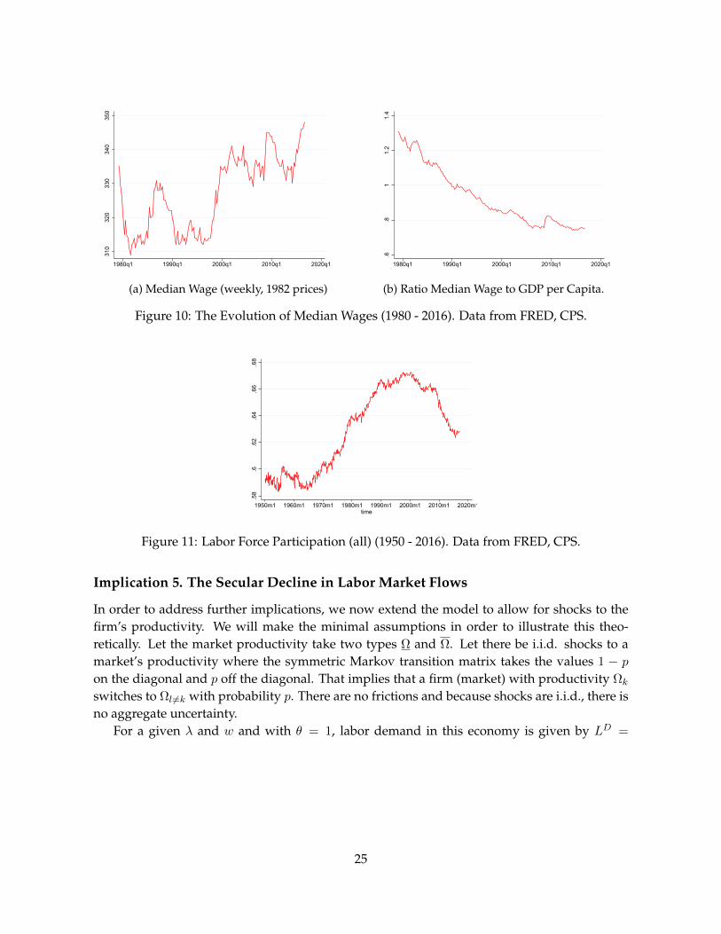
We can now relate these two theoretical findings to the empirical evidence of the followingtwo implications of the rise in market power. There is ample evidence of low wage stagnationin the last few decades that is consistent with the finding in Result 1. Figure 10a plots theweekly median wage, in constant 1982 prices. There has been little or no change in the medianwage since the 1980s. In the presence of economic growth, that means that the share of medianwages of GDP per capita has decreased. Figure 10b plots the ratio of median wages to GDP percapita. There has been a secular decline in this ratio from 1.3 in 1980 to 0.75 now.

This is not simply a artifact of how the distribution of earnings is spread over the life cycle.31

Implication 4. The Secular Decline in Labor Force Participation

Figure 11 plots the labor force participation rate for the US economy since 1950. There is asharp decline since the mid 1990s. It appears that this does not fully coincide with the thetiming of the rise in market power. However, the sharp increase in the labor force since the1960s is driven by the increased female participation. This has led to an outward shift of thelabor supply. This trend has leveled off in the mid 1990s, which is consistent with the fact thatwe start to see the impact of a decrease in the total labor force participation due to the rise inmarket power.

31Say for example that due to fact that the age-earnings profile has become steeper and with more variance, themedian wage is lower. Guvenen, Kaplan, Song, and Weidner (2017) show that the same is true for life time earnings.

24

310

320

330

340

350

1980q1 1990q1 2000q1 2010q1 2020q1

(a) Median Wage (weekly, 1982 prices)

.6.8

11.

21.

4

1980q1 1990q1 2000q1 2010q1 2020q1

(b) Ratio Median Wage to GDP per Capita.

Figure 10: The Evolution of Median Wages (1980 - 2016). Data from FRED, CPS.

.58

.6.6

2.6

4.6

6.6

8

1950m1 1960m1 1970m1 1980m1 1990m1 2000m1 2010m1 2020m1time

Figure 11: Labor Force Participation (all) (1950 - 2016). Data from FRED, CPS.

Implication 5. The Secular Decline in Labor Market Flows

In order to address further implications, we now extend the model to allow for shocks to thefirm’s productivity. We will make the minimal assumptions in order to illustrate this theo-retically. Let the market productivity take two types Ω and Ω. Let there be i.i.d. shocks to amarket’s productivity where the symmetric Markov transition matrix takes the values 1 − p

on the diagonal and p off the diagonal. That implies that a firm (market) with productivity Ωk

switches to Ωl 6=k with probability p. There are no frictions and because shocks are i.i.d., there isno aggregate uncertainty.

For a given λ and w and with θ = 1, labor demand in this economy is given by LD =

25

12L+ 1

2L. In every period, the amount of labor reallocation ∆L is32

∆L = p

∣∣∣∣12L− 1

2L

∣∣∣∣ = p1

2(1 + λ)b

∣∣∣∣ aΩ − w

Ω2 −

a

Ω+

w

Ω2

∣∣∣∣ . (34)

It follows immediately that labor reallocation is decreasing in λ:

∂∆L

∂λ= −p 1

2(1 + λ)2b

∣∣∣∣ aΩ − w

Ω2 −

a

Ω+

w

Ω2

∣∣∣∣ < 0. (35)

This is true for constant w (elastic labor supply). Given linear demand, this result holds moregenerally if also supply is linear (or concave), and under those conditions we can establish thefollowing result.

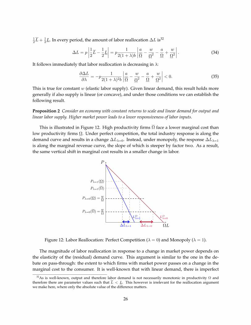
Proposition 2 Consider an economy with constant returns to scale and linear demand for output andlinear labor supply. Higher market power leads to a lower responsiveness of labor inputs.

This is illustrated in Figure 12. High productivity firms Ω face a lower marginal cost thanlow productivity firms Ω. Under perfect competition, the total industry response is along thedemand curve and results in a change ∆Lλ=0. Instead, under monopoly, the response ∆Lλ=1

is along the marginal revenue curve, the slope of which is steeper by factor two. As a result,the same vertical shift in marginal cost results in a smaller change in labor.

ΩL

P

LDλ=0

∆Lλ=0

LDλ=1

∆Lλ=1

wΩ

wΩ

Pλ=0(Ω) =

Pλ=0(Ω) =

Pλ=1(Ω)

Pλ=1(Ω)

Figure 12: Labor Reallocation: Perfect Competition (λ = 0) and Monopoly (λ = 1).

The magnitude of labor reallocation in response to a change in market power depends onthe elasticity of the (residual) demand curve. This argument is similar to the one in the de-bate on pass-through: the extent to which firms with market power passes on a change in themarginal cost to the consumer. It is well-known that with linear demand, there is imperfect

32As is well-known, output and therefore labor demand is not necessarily monotonic in productivity Ω andtherefore there are parameter values such that L < L. This however is irrelevant for the reallocation argumentwe make here, where only the absolute value of the difference matters.

26

passthrough (see for example Melitz and Ottaviano (2008)), but not with constant elasticity de-mand.33 Eventually it is an empirical question what the elasticity of demand and supply is,and therefore whether and how much pass through there is. There is quite a bit of evidence ofincomplete passthrough, most of which comes from the effect of changes in the exchange rateor reduction in tariffs, see Campa and Goldberg (2005) and De Loecker, Goldberg, Khandelwal,and Pavcnik (2016).

We have treated wagesw as exogenous, which is equivalent to perfectly elastic labor supply.Whenever labor supply is upward sloping (as in Figure 9), a change in λ also affects wages. It iseasily verified that an increase in market power λ still leads to a decrease in labor reallocationas long as labor supply is not too convex.34

The decrease in labor reallocation as a result of the increase in market power (Result 2) formsthe basis for two macroeconomic implications. There has been a secular decline in businessdynamics broadly defined. This is manifest in several observed outcomes, most notably inthe evolution of labor market flows and in the evolution of migration rates. The likelihood ofswitching jobs and the flows in and out of unemployment have dropped (and as a result theduration of employment has increased).

.015

.025

.03

.04

.06

.08

tota

l

1975q1 1980q1 1985q1 1990q1 1995q1 2000q1 2005q1 2010q1 2015q1dq

(UE+NE)/( U+N) (left axis) ee (right axis)

(a) Labor Market Flows (1976-2016).

.01

.015

.02

.025

.03

.035

1960 1965 1970 1975 1980 1985 1990 1995 2000 2005 2010 2015

Migration Rates

(b) Migration, between MSA’s (1962 - 2016).

Figure 13: Labor Reallocation (1976-2016). CPS data.

Figure 13a shows the evolution of labor market flows based on CPS data. The sharpestdecline is in the Employment-to-Employment (EE) flows, though we only have data on EEflows since 1996. The probability for an employed worker to switch to another job has gonedown from 2.9% to 1.8%. There is also a decrease in the flow rate of the unemployed and thosenot in the labor force from 6.5% in 1980 to 4.7% now.

Our model in conjunction with the rise in market power provides a mechanism for the

33Even with CES demand, passthrough can be incomplete depending on the preference aggregation. Yeh (2017)for example analyzes the responsiveness of large firms to i.i.d. shocks and he uses a Kimball aggregator of the CESdemand.

34Or when wages are perfectly inelastic. In that case there is zero labor reallocation.

27

decline in job flows.35 The simplified static model is meant to illustrate the role of market powerin a setting with full blown firm dynamics as in Jovanovic (1982) and Hopenhayn (1992). Firmsthat receive positive productivity shocks augment output by augmenting inputs such as theirlabor force, and they reduce output by reducing inputs when a negative shock hits.36

An obvious reason why job flows could have decreased is that the volatility of productiv-ity shocks (p in our stylized model) has decreased over time. Then even with constant marketpower, we would see lower job flows. However, as Decker, Haltiwanger, Jarmin, and Mi-randa (2014) find for the US economy, the volatility of shocks has not decreased in the last fewdecades. If anything, it has increased. But as they point out, it is not the volatility of the shocksthat has decreased, but rather the responsiveness of firm’s output and labor force decisions tothe existing shocks.37

If the distribution of idiosyncratic shocks remains unchanged, then the responsiveness ofthe labor input and therefore the transmission of shocks will lead to a decrease in job flows asmarket power increases. This can illustrate the pattern of decreased job flows observed in theUS labor market and plotted in Figure 13a.

Observe that this is consistent with what we find on the evolution of the cross-sectionalstandard deviation of the noise term reported in Figure 4. While there is an increase in thestandard deviation of sales, the standard deviation of employment is much more moderate,and even declines while that of sales increases. This confirms the finding by Decker, Halti-wanger, Jarmin, and Miranda (2014) that the transmission of the shocks to labor has becomemore attenuated over time.

Implication 6. The Secular Decline in Migration Rates

Finally, for the same reason as the decrease in the job flow rates, the transmission of shockshas implications on the job relocation choices across different local labor markets. There hasbeen a marked decrease in interstate migration as well as the migration between metropolitanareas. Figure 13b shows that relocation rate has nearly halved, from around 3% in 1980 to 1.5%now.38 If firms are based in different local labor markets and a fixed fraction of all job relocationdecisions are between local labor markets, then lower job flow rates will automatically give riseto lower migration rates.

35There are several potential alternative explanations for the decline in job flows: demographic change (agingworkforce, Fallick, Fleischman, and Pingle (2010)), a more skilled workforce, lower population growth, decreasedlabor supply (Karahan, Pugsley, and Sahin (2016)), technological change (Eeckhout and Weng (2017)), changedvolatility of production, and government policy (such as employment protection legislation, licensing,...; see Davisand Haltiwanger (2014)). Hyatt and Spletzer (2013) show that demographic changes can explain at most one thirdof the decline in job flows.

36Recent work by Baqaee and Farhi (2017) draws attention to the fact that firm-level productivity shocks cangive rise to a nonlinear impact on macroeconomic outcomes. For example, models with network linkages such asGabaix (2011) give rise to such non-linearities. So does market power in the presence of incomplete passthrough aswe show in this section.

37Independent evidence at business cycle frequency by Berger and Vavra (2017) establishes that the volatility ofprices is due to firms’ time-varying responsiveness to shocks rather than to the time-varying nature of the shocksthemselves. Their identification strategy is derived from the exchange rate passthrough of volatility on prices.

38See also Kaplan and Schulhofer-Wohl (2012), amongst others.

28

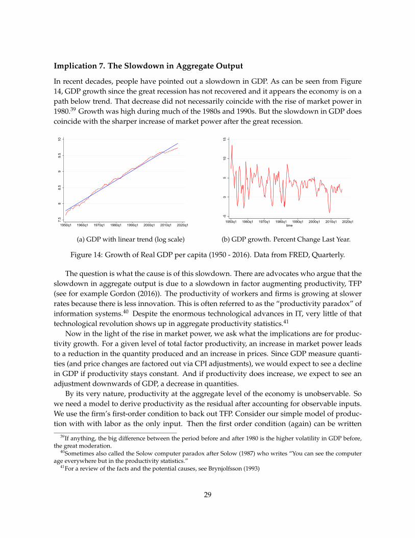
Implication 7. The Slowdown in Aggregate Output

In recent decades, people have pointed out a slowdown in GDP. As can be seen from Figure14, GDP growth since the great recession has not recovered and it appears the economy is on apath below trend. That decrease did not necessarily coincide with the rise of market power in1980.39 Growth was high during much of the 1980s and 1990s. But the slowdown in GDP doescoincide with the sharper increase of market power after the great recession.

7.5

88.

59

9.5

10

1950q1 1960q1 1970q1 1980q1 1990q1 2000q1 2010q1 2020q1

(a) GDP with linear trend (log scale)

-50

510

151950q1 1960q1 1970q1 1980q1 1990q1 2000q1 2010q1 2020q1

time

(b) GDP growth. Percent Change Last Year.

Figure 14: Growth of Real GDP per capita (1950 - 2016). Data from FRED, Quarterly.

The question is what the cause is of this slowdown. There are advocates who argue that theslowdown in aggregate output is due to a slowdown in factor augmenting productivity, TFP(see for example Gordon (2016)). The productivity of workers and firms is growing at slowerrates because there is less innovation. This is often referred to as the “productivity paradox” ofinformation systems.40 Despite the enormous technological advances in IT, very little of thattechnological revolution shows up in aggregate productivity statistics.41

Now in the light of the rise in market power, we ask what the implications are for produc-tivity growth. For a given level of total factor productivity, an increase in market power leadsto a reduction in the quantity produced and an increase in prices. Since GDP measure quanti-ties (and price changes are factored out via CPI adjustments), we would expect to see a declinein GDP if productivity stays constant. And if productivity does increase, we expect to see anadjustment downwards of GDP, a decrease in quantities.

By its very nature, productivity at the aggregate level of the economy is unobservable. Sowe need a model to derive productivity as the residual after accounting for observable inputs.We use the firm’s first-order condition to back out TFP. Consider our simple model of produc-tion with with labor as the only input. Then the first order condition (again) can be written

39If anything, the big difference between the period before and after 1980 is the higher volatility in GDP before,the great moderation.

40Sometimes also called the Solow computer paradox after Solow (1987) who writes “You can see the computerage everywhere but in the productivity statistics.”

41For a review of the facts and the potential causes, see Brynjolfsson (1993)

29

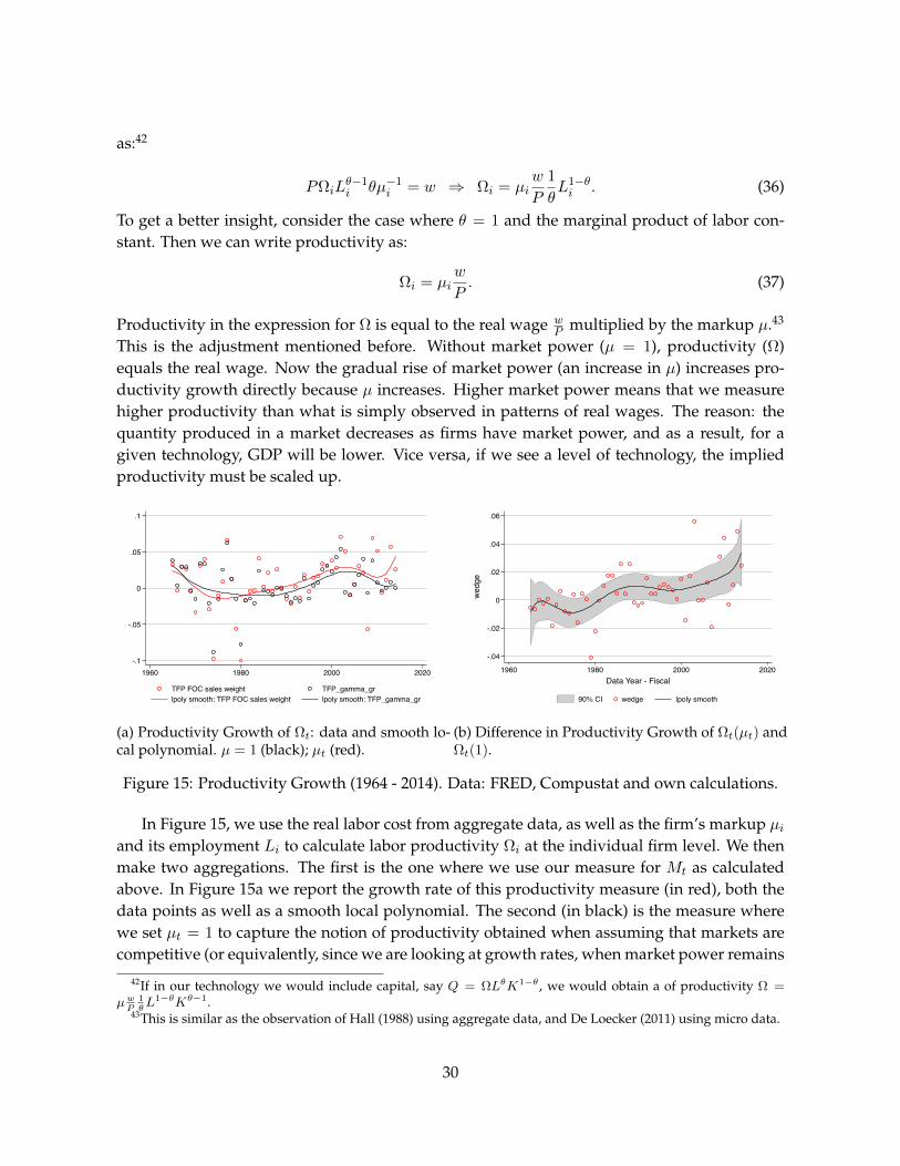
as:42

PΩiLθ−1i θµ−1

i = w ⇒ Ωi = µiw

P

1

θL1−θi . (36)

To get a better insight, consider the case where θ = 1 and the marginal product of labor con-stant. Then we can write productivity as:

Ωi = µiw

P. (37)

Productivity in the expression for Ω is equal to the real wage wP multiplied by the markup µ.43

This is the adjustment mentioned before. Without market power (µ = 1), productivity (Ω)equals the real wage. Now the gradual rise of market power (an increase in µ) increases pro-ductivity growth directly because µ increases. Higher market power means that we measurehigher productivity than what is simply observed in patterns of real wages. The reason: thequantity produced in a market decreases as firms have market power, and as a result, for agiven technology, GDP will be lower. Vice versa, if we see a level of technology, the impliedproductivity must be scaled up.

-.1

-.05

0

.05

.1

1960 1980 2000 2020

TFP FOC sales weight TFP_gamma_grlpoly smooth: TFP FOC sales weight lpoly smooth: TFP_gamma_gr

(a) Productivity Growth of Ωt: data and smooth lo-cal polynomial. µ = 1 (black); µt (red).

-.04

-.02

0

.02

.04

.06

wed

ge

1960 1980 2000 2020Data Year - Fiscal

90% CI wedge lpoly smooth

(b) Difference in Productivity Growth of Ωt(µt) andΩt(1).

Figure 15: Productivity Growth (1964 - 2014). Data: FRED, Compustat and own calculations.

In Figure 15, we use the real labor cost from aggregate data, as well as the firm’s markup µiand its employment Li to calculate labor productivity Ωi at the individual firm level. We thenmake two aggregations. The first is the one where we use our measure for Mt as calculatedabove. In Figure 15a we report the growth rate of this productivity measure (in red), both thedata points as well as a smooth local polynomial. The second (in black) is the measure wherewe set µt = 1 to capture the notion of productivity obtained when assuming that markets arecompetitive (or equivalently, since we are looking at growth rates, when market power remains

42If in our technology we would include capital, say Q = ΩLθK1−θ , we would obtain a of productivity Ω =µwP

1θL1−θKθ−1.

43This is similar as the observation of Hall (1988) using aggregate data, and De Loecker (2011) using micro data.

30

unchanged). We believe that productivity growth should capture the impact of markups andwe find that productivity growth is higher since 1980 than when it does not incorporate theinfluence of changing markups. From Figure 15b it is also evident that the difference betweenthe two measures widens.

More importantly, we find that except for a dip around the great recession, productivityactually increases and hovers around 3 to 4% after the 2000. Without accounting for the increasein market power, we find a decrease in measured productivity. This indicates that properlyaccounting for market power, there is no productivity slowdown but instead an increase inproductivity.

5 Concluding Remarks

Using micro data on the accounts of publicly traded firms in the US starting in 1950, wefind that markups have been relatively constant between 1950 and 1980 at around 20% abovemarginal cost. From 1980 onwards, there has been marked change in this pattern with markupssteadily rising from 18% to nearly 67% in 2014, a three and a half fold increase.

We have documented the properties of this rise, which is mainly due to a change withinindustry, and which can be attributed mostly to the increase of markup of the firms with thehighest markups already. Markups tend to be larger in smaller firms, but this seems to be duemainly to a composition effects across industries as this disappears when we decompose themarkup at the fine industry level.

We use this increase to investigate the implications this has for secular macroeconomictrends in the last decades: 1. decrease in labor share; 2. decrease in capital share; 3. decrease inlow skill wages; 4. decrease in labor force participation; 5. decrease in labor flows; 6. decreasein migration rates; 7. slowdown in output and GDP.

There are of course other secular trends that happen to coincide with the increase in marketpower: 1. decrease in startup rate of new firms44 due to higher barriers erected by incumbents;2. decrease in the long term interest rate45 due to the fall in demand for capital (due to quantityreduction of firms with market power) and an increase in the supply of capital (due to higherprofits); 3. the increase in wage inequality46 from to the decrease in low skill wages as docu-mented above together with an increase in skilled wages due to profit sharing by managers; 4.the great moderation, or the idea that output fluctuations have decreased since 1980,47 has lostappeal since the great recession, but which is still very much observed in the data, especially inthe last decade, with of course, the notable exception of 2008.

As we have shown, with incomplete pass-through the same individual firm level productiv-

44See amongst others Davis, Haltiwanger, Jarmin, and Miranda (2007) and Karahan, Pugsley, and Sahin (2016)45See for example Caballero, Farhi, and Gourinchas (2017). This is often also linked to Greenspan’s conundrum,

the inability of the Federal Reserve to increase the long term Treasury yield despite sizable increases in the federalfunds rate.

46See amongst many others Autor, Katz, and Kearney (2008).47See for example Bernanke (2004) and Davis and Kahn (2008). To get a visual idea of the difference in output

volatility before and after 1980, simply look at Figure 14b.

31

ity shocks lead to lower output adjustments. There is evidence however that the transmissionof aggregate shocks is also incomplete. As a result, higher market power would translate insmaller aggregate fluctuations GDP in response to aggregate shocks as well. While we believethat each of these four secular trends are as important as, if not more important than, the oneswe have analyzed, we leave them as a priority for future research.

There are two profound policy consequences that result from the rise in market power.The first relates to inflation. Relative to a scenario without a rise market power and with thesame evolution of technology, prices would have gone up by 1% per year (42% over 35 years,from 1.18 to 1.67). This implies that inflation has been higher than it would have been withoutthe rise in market power. This is surprising given the low inflation rates in the last decades– and particularly low ones since the great recession. Of course, monetary policy is not theappropriate policy tool to remedy that source of inflation. That would be the prerogative ofanti-trust policy.

The second consequence pertains to the value of the stock market. Stocks prices reflectthe discounted flow of dividends and thus profits. The stock market under market power istherefore overvalued relative to a competitive economy. If investors believe that the currentprofit level that is four times higher than in 1980 is permanent, then we would expect that thestock market capitalization would be four time higher than under perfect competition. Thatwould put the Dow Jones at 5,500 instead of its nearly 22,000 level today. Of course, that is anaive calculation since market capitalization also reflects the extensive margin, the total valueof goods sold, and that decreases with market power. How big the effect of market power is onthe stock market value depends on the elasticity of demand. Note also that the stock marketcan go up if output deceases, for example when productivity growth is zero and market powerand hence profits increase. In the presence of market power, the stock market is therefore not agood gauge of an economy’s output.

While we have focused on the consequences of the rise in market power, in this paper wehave remained silent on the causes. Especially when it comes to finding remedies, it is essentialto understand the causes. We limit ourselves to listing a number of candidate explanations: therise of merger & acquisition activity (Figure B.9 in the Appendix), deregulation, the highershare of network goods, the increase in wholesale transaction (Ganapati (2016)), private equity,improved product differentiation, increased vertical and financial integration of competitors.A common factor in each of these is technology. Rapid technological change allows firms tobetter create and preserve situations of market power.

Markups are reaching heights multiple times higher than ever seen, at least since the secondworld war when our data start. It is open to speculation whether this trend will continue, butfor now there are no signs that markups will decrease substantially any time soon.

32

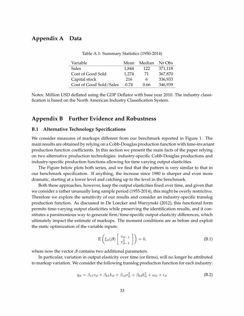
Appendix A Data

Table A.1: Summary Statistics (1950-2014)

Variable Mean Median Nr ObsSales 1,844 122 371,118Cost of Good Sold 1,274 71 367,870Capital stock 216 6 336,933Cost of Good Sold/Sales 0.74 0.66 346,939

Notes: Million USD deflated using the GDP Deflator with base year 2010. The industry classi-fication is based on the North American Industry Classification System.

Appendix B Further Evidence and Robustness

B.1 Alternative Technology Specifications

We consider measures of markups different from our benchmark reported in Figure 1. Themain results are obtained by relying on a Cobb-Douglas production function with time-invariantproduction function coefficients. In this section we present the main facts of the paper relyingon two alternative production technologies: industry-specific Cobb-Douglas productions andindustry-specific production functions allowing for time varying output elasticities.

The Figure below plots both series, and we find that the pattern is very similar to that inour benchmark specification. If anything, the increase since 1980 is sharper and even moredramatic, starting at a lower level and catching up to the level in the benchmark.

Both these approaches, however, keep the output elasticities fixed over time, and given thatwe consider a rather unusually long sample period (1955-2014), this might be overly restrictive.Therefore we explore the sensitivity of our results and consider an industry-specific translogproduction function. As discussed in De Loecker and Warzynski (2012), this functional formpermits time-varying output elasticities while preserving the identification results, and it con-stitutes a parsimonious way to generate firm/time-specific output elasticity differences, whichultimately impact the estimate of markups. The moment conditions are as before and exploitthe static optimization of the variable inputs:

E(ξit(β)

[vit−1

v2it−1

])= 0, (B.1)

where now the vector β contains two additional parameters.In particular, variation in output elasticity over time (or firms), will no longer be attributed

to markup variation. We consider the following translog production function for each industry:

qit = βv1vit + βk1kit + βv2v2it + βk2k

2it + ωit + εit (B.2)

33

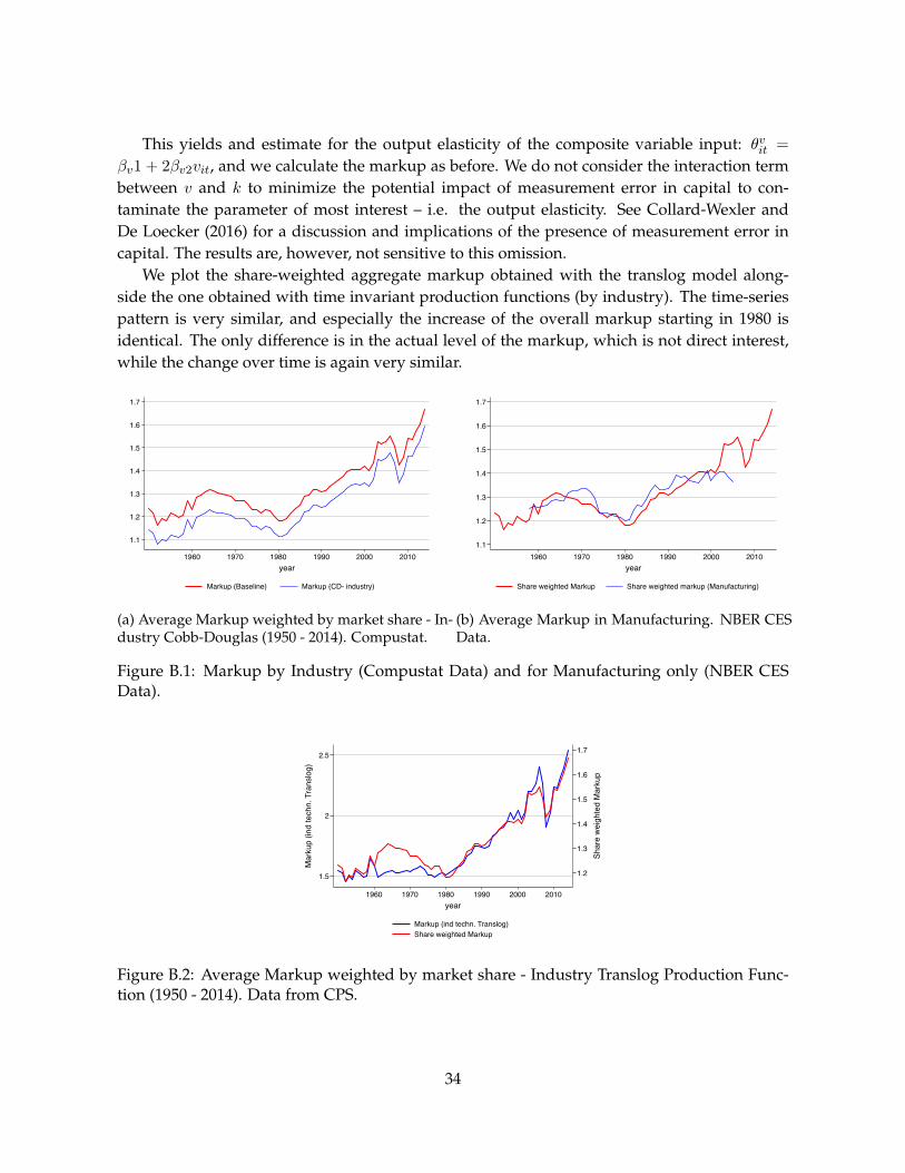
This yields and estimate for the output elasticity of the composite variable input: θvit =

βv1 + 2βv2vit, and we calculate the markup as before. We do not consider the interaction termbetween v and k to minimize the potential impact of measurement error in capital to con-taminate the parameter of most interest – i.e. the output elasticity. See Collard-Wexler andDe Loecker (2016) for a discussion and implications of the presence of measurement error incapital. The results are, however, not sensitive to this omission.

We plot the share-weighted aggregate markup obtained with the translog model along-side the one obtained with time invariant production functions (by industry). The time-seriespattern is very similar, and especially the increase of the overall markup starting in 1980 isidentical. The only difference is in the actual level of the markup, which is not direct interest,while the change over time is again very similar.

1.1

1.2

1.3

1.4

1.5

1.6

1.7

1960 1970 1980 1990 2000 2010year

Markup (Baseline) Markup (CD- industry)

(a) Average Markup weighted by market share - In-dustry Cobb-Douglas (1950 - 2014). Compustat.

1.1

1.2

1.3

1.4

1.5

1.6

1.7

1960 1970 1980 1990 2000 2010year

Share weighted Markup Share weighted markup (Manufacturing)

(b) Average Markup in Manufacturing. NBER CESData.

Figure B.1: Markup by Industry (Compustat Data) and for Manufacturing only (NBER CESData).

1.2

1.3

1.4

1.5

1.6

1.7

Shar

e w

eigh

ted

Mar

kup

1.5

2

2.5

Mar

kup

(ind

tech

n. T

rans

log)

1960 1970 1980 1990 2000 2010year

Markup (ind techn. Translog)Share weighted Markup

Figure B.2: Average Markup weighted by market share - Industry Translog Production Func-tion (1950 - 2014). Data from CPS.

34

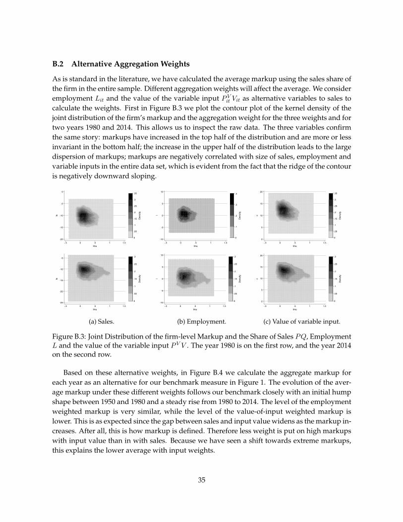
B.2 Alternative Aggregation Weights

As is standard in the literature, we have calculated the average markup using the sales share ofthe firm in the entire sample. Different aggregation weights will affect the average. We consideremployment Lit and the value of the variable input P Vit Vit as alternative variables to sales tocalculate the weights. First in Figure B.3 we plot the contour plot of the kernel density of thejoint distribution of the firm’s markup and the aggregation weight for the three weights and fortwo years 1980 and 2014. This allows us to inspect the raw data. The three variables confirmthe same story: markups have increased in the top half of the distribution and are more or lessinvariant in the bottom half; the increase in the upper half of the distribution leads to the largedispersion of markups; markups are negatively correlated with size of sales, employment andvariable inputs in the entire data set, which is evident from the fact that the ridge of the contouris negatively downward sloping.

-20

-15

-10

-5

0

ls

-.5 0 .5 1 1.5lmu

0

.05

.1

.15

.2

.25

.3

.35

Density

-25

-20

-15

-10

-5

ls

-.5 0 .5 1 1.5lmu

0

.05

.1

.15

.2

.25

.3

Density

(a) Sales.

-10

-5

0

5

10

l

-.5 0 .5 1 1.5lmu

0

.1

.2

.3

.4

Density

-10

-5

0

5

10

l

-.5 0 .5 1 1.5lmu

0

.05

.1

.15

.2

.25

.3

Density

(b) Employment.

0

5

10

15

20

c

-.5 0 .5 1 1.5lmu

0

.05

.1

.15

.2

.25

.3

.35

Density

0

5

10

15

20c

-.5 0 .5 1 1.5lmu

0

.05

.1

.15

.2

.25

.3

Density

(c) Value of variable input.

Figure B.3: Joint Distribution of the firm-level Markup and the Share of Sales PQ, EmploymentL and the value of the variable input P V V . The year 1980 is on the first row, and the year 2014on the second row.

Based on these alternative weights, in Figure B.4 we calculate the aggregate markup foreach year as an alternative for our benchmark measure in Figure 1. The evolution of the aver-age markup under these different weights follows our benchmark closely with an initial humpshape between 1950 and 1980 and a steady rise from 1980 to 2014. The level of the employmentweighted markup is very similar, while the level of the value-of-input weighted markup islower. This is as expected since the gap between sales and input value widens as the markup in-creases. After all, this is how markup is defined. Therefore less weight is put on high markupswith input value than in with sales. Because we have seen a shift towards extreme markups,this explains the lower average with input weights.

35

1.2

1.3

1.4

1.5

1.6

1.7Sh

are

(labo

r) W

eigh

ted

Mar

kup

1960 1970 1980 1990 2000 2010year

(a) Employment.

1.1

1.15

1.2

1.25

1.3

Shar

e (V

aria

ble

Inpu

ts) W

eigh

ted

Mar

kup

1960 1970 1980 1990 2000 2010year

(b) Value of variable input.

Figure B.4: Share weighted Markup: alternative weights: Employment and the Value of thevariable input.

B.3 Decomposition of change in markup at different industry level aggregation

Markup ∆ Markup ∆ Within ∆ Between ∆ Realloc.2-digit industry

1971 1.268 -0.028 -0.025 0.041 -0.0321981 1.181 -0.087 -0.085 0.016 -0.0171991 1.315 0.134 0.123 0.016 -0.0062001 1.400 0.085 0.089 0.006 -0.010

3-digit industry1971 1.268 -0.028 -0.026 0.034 -0.0271981 1.181 -0.087 -0.084 0.022 -0.0251991 1.315 0.134 0.104 0.033 -0.0032001 1.400 0.085 0.089 -0.003 -0.004

4-digit industry1971 1.268 -0.028 -0.028 0.035 -0.0351981 1.181 -0.087 -0.089 0.026 -0.0241991 1.315 0.134 0.090 0.045 -0.0022001 1.400 0.085 0.061 0.011 0.010

Table B.1: Decomposition of 10 year change in Markup at different industry levels.

B.4 Markups using aggregate-level data

In the literature (first and foremost, see Hall (1988)) the analysis of markups has been per-formed using aggregate data. In this section we aim to achieve two goals. First, we want toperform the analysis on different data from ours that covers the entire economy, not just the

36

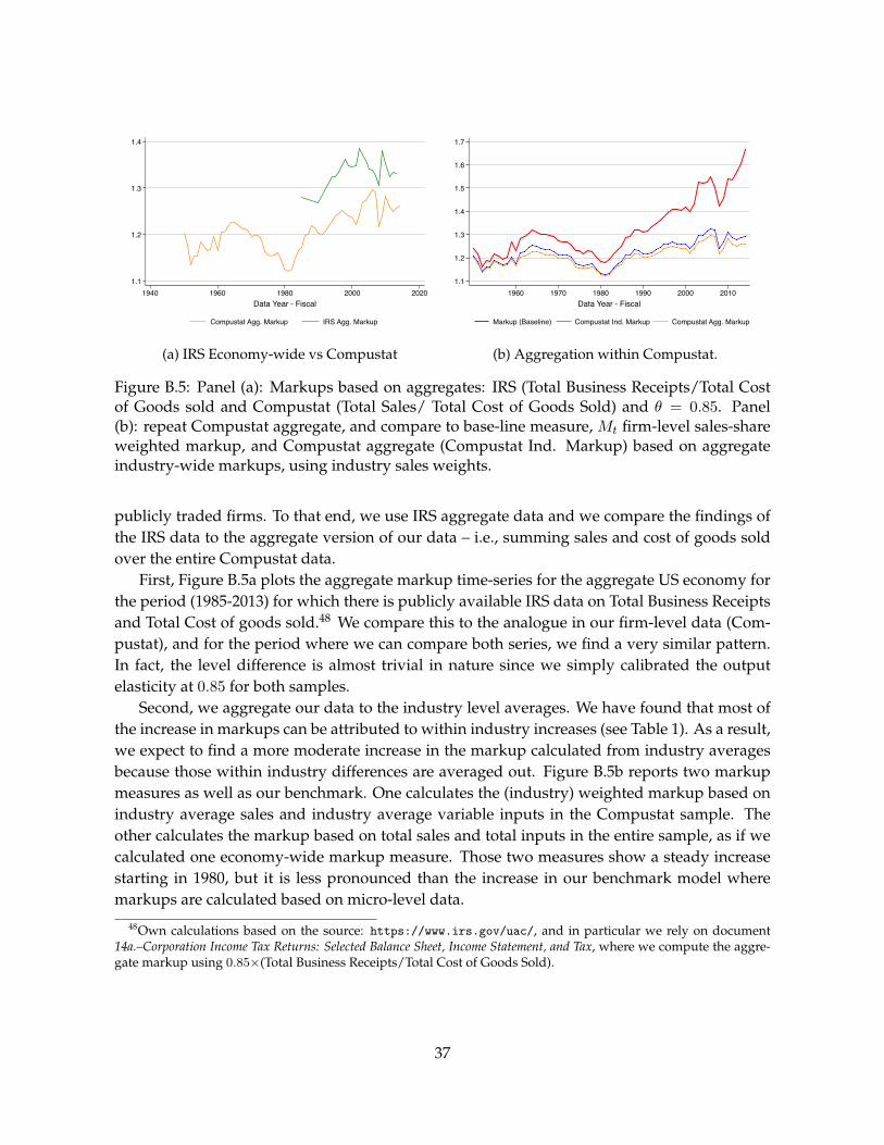
1.1

1.2

1.3

1.4

1940 1960 1980 2000 2020Data Year - Fiscal

Compustat Agg. Markup IRS Agg. Markup

(a) IRS Economy-wide vs Compustat

1.1

1.2

1.3

1.4

1.5

1.6

1.7

1960 1970 1980 1990 2000 2010Data Year - Fiscal

Markup (Baseline) Compustat Ind. Markup Compustat Agg. Markup

(b) Aggregation within Compustat.

Figure B.5: Panel (a): Markups based on aggregates: IRS (Total Business Receipts/Total Costof Goods sold and Compustat (Total Sales/ Total Cost of Goods Sold) and θ = 0.85. Panel(b): repeat Compustat aggregate, and compare to base-line measure, Mt firm-level sales-shareweighted markup, and Compustat aggregate (Compustat Ind. Markup) based on aggregateindustry-wide markups, using industry sales weights.

publicly traded firms. To that end, we use IRS aggregate data and we compare the findings ofthe IRS data to the aggregate version of our data – i.e., summing sales and cost of goods soldover the entire Compustat data.

First, Figure B.5a plots the aggregate markup time-series for the aggregate US economy forthe period (1985-2013) for which there is publicly available IRS data on Total Business Receiptsand Total Cost of goods sold.48 We compare this to the analogue in our firm-level data (Com-pustat), and for the period where we can compare both series, we find a very similar pattern.In fact, the level difference is almost trivial in nature since we simply calibrated the outputelasticity at 0.85 for both samples.

Second, we aggregate our data to the industry level averages. We have found that most ofthe increase in markups can be attributed to within industry increases (see Table 1). As a result,we expect to find a more moderate increase in the markup calculated from industry averagesbecause those within industry differences are averaged out. Figure B.5b reports two markupmeasures as well as our benchmark. One calculates the (industry) weighted markup based onindustry average sales and industry average variable inputs in the Compustat sample. Theother calculates the markup based on total sales and total inputs in the entire sample, as if wecalculated one economy-wide markup measure. Those two measures show a steady increasestarting in 1980, but it is less pronounced than the increase in our benchmark model wheremarkups are calculated based on micro-level data.

48Own calculations based on the source: https://www.irs.gov/uac/, and in particular we rely on document14a.–Corporation Income Tax Returns: Selected Balance Sheet, Income Statement, and Tax, where we compute the aggre-gate markup using 0.85×(Total Business Receipts/Total Cost of Goods Sold).

37

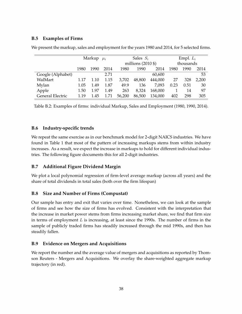
B.5 Examples of Firms

We present the markup, sales and employment for the years 1980 and 2014, for 5 selected firms.

Markup µi Sales Si Empl. Limillions (2010 $) thousands

1980 1990 2014 1980 1990 2014 1980 1990 2014Google (Alphabet) 2.71 60,600 53WalMart 1.17 1.10 1.15 3,702 48,800 444,000 27 328 2,200Mylan 1.05 1.49 1.87 49.9 136 7,093 0.23 0.51 30Apple 1.50 1.97 1.49 263 8,324 168,000 1 14 97General Electric 1.19 1.45 1.71 56,200 86,500 134,000 402 298 305

Table B.2: Examples of firms: individual Markup, Sales and Employment (1980, 1990, 2014).

B.6 Industry-specific trends

We repeat the same exercise as in our benchmark model for 2-digit NAICS industries. We havefound in Table 1 that most of the pattern of increasing markups stems from within industryincreases. As a result, we expect the increase in markups to hold for different individual indus-tries. The following figure documents this for all 2-digit industries.

B.7 Additional Figure Dividend Margin

We plot a local polynomial regression of firm-level average markup (across all years) and theshare of total dividends in total sales (both over the firm lifespan)

B.8 Size and Number of Firms (Compustat)

Our sample has entry and exit that varies over time. Nonetheless, we can look at the sampleof firms and see how the size of firms has evolved. Consistent with the interpretation thatthe increase in market power stems from firms increasing market share, we find that firm sizein terms of employment L is increasing, at least since the 1990s. The number of firms in thesample of publicly traded firms has steadily increased through the mid 1990s, and then hassteadily fallen.

B.9 Evidence on Mergers and Acquisitions

We report the number and the average value of mergers and acquisitions as reported by Thom-son Reuters - Mergers and Acquisitions. We overlay the share-weighted aggregate markuptrajectory (in red).

38

.001

.002

.003

.004

.005

.006

shar

e_in

d2

11.251.5

1.752

2.252.5

2.753

3.25

1940 1960 1980 2000 2020year

MARKUP_IND2Markupshare_ind2

Markup and Market share: 11

.02

.03

.04

.05

shar

e_in

d2

11.251.5

1.752

2.252.5

2.753

3.25

1940 1960 1980 2000 2020year

MARKUP_IND2Markupshare_ind2

Markup and Market share: 21

0

.02

.04

.06

.08

shar

e_in

d2

11.251.5

1.752

2.252.5

2.753

3.25

1940 1960 1980 2000 2020year

MARKUP_IND2Markupshare_ind2

Markup and Market share: 22

0

.002

.004

.006

.008

.01

shar

e_in

d2

11.251.5

1.752

2.252.5

2.753

3.25

1940 1960 1980 2000 2020year

MARKUP_IND2Markupshare_ind2

Markup and Market share: 23

.04

.06

.08

.1

shar

e_in

d2

11.251.5

1.752

2.252.5

2.753

3.25

1940 1960 1980 2000 2020year

MARKUP_IND2Markupshare_ind2

Markup and Market share: 31

.15

.2

.25

.3

.35

shar

e_in

d2

11.251.5

1.752

2.252.5

2.753

3.25

1940 1960 1980 2000 2020year

MARKUP_IND2Markupshare_ind2

Markup and Market share: 32

.15

.2

.25

.3

.35

.4

shar

e_in

d2

11.251.5

1.752

2.252.5

2.753

3.25

1940 1960 1980 2000 2020year

MARKUP_IND2Markupshare_ind2

Markup and Market share: 33

.01

.02

.03

.04

.05

shar

e_in

d2

11.251.5

1.752

2.252.5

2.753

3.25

1940 1960 1980 2000 2020year

MARKUP_IND2Markupshare_ind2

Markup and Market share: 42

.03

.04

.05

.06

.07

shar

e_in

d2

11.251.5

1.752

2.252.5

2.753

3.25

1940 1960 1980 2000 2020year

MARKUP_IND2Markupshare_ind2

Markup and Market share: 44

.02

.03

.04

.05

shar

e_in

d2

11.251.5

1.752

2.252.5

2.753

3.25

1940 1960 1980 2000 2020year

MARKUP_IND2Markupshare_ind2

Markup and Market share: 45

.01

.02

.03

.04

.05

shar

e_in

d2

11.251.5

1.752

2.252.5

2.753

3.25

1940 1960 1980 2000 2020year

MARKUP_IND2Markupshare_ind2

Markup and Market share: 48

0

.002

.004

.006

.008

.01

shar

e_in

d2

11.251.5

1.752

2.252.5

2.753

3.25

1940 1960 1980 2000 2020year

MARKUP_IND2Markupshare_ind2

Markup and Market share: 49

.02

.04

.06

.08

.1

shar

e_in

d2

11.251.5

1.752

2.252.5

2.753

3.25

1940 1960 1980 2000 2020year

MARKUP_IND2Markupshare_ind2

Markup and Market share: 51

0

.05

.1

.15

.2

shar

e_in

d2

11.251.5

1.752

2.252.5

2.753

3.25

1940 1960 1980 2000 2020year

MARKUP_IND2Markupshare_ind2

Markup and Market share: 52

.002

.004

.006

.008

.01

shar

e_in

d2

11.251.5

1.752

2.252.5

2.753

3.25

1940 1960 1980 2000 2020year

MARKUP_IND2Markupshare_ind2

Markup and Market share: 53

0

.01

.02

.03

shar

e_in

d2

11.251.5

1.752

2.252.5

2.753

3.25

1940 1960 1980 2000 2020year

MARKUP_IND2Markupshare_ind2

Markup and Market share: 54

0

.002

.004

.006

.008

.01

shar

e_in

d2

11.251.5

1.752

2.252.5

2.753

3.25

1940 1960 1980 2000 2020year

MARKUP_IND2Markupshare_ind2

Markup and Market share: 56

0

.0002

.0004

.0006

.0008

.001

shar

e_in

d2

11.251.5

1.752

2.252.5

2.753

3.25

1960 1980 2000 2020year

MARKUP_IND2Markupshare_ind2

Markup and Market share: 61

0

.002

.004

.006

.008

shar

e_in

d2

11.251.5

1.752

2.252.5

2.753

3.25

1960 1980 2000 2020year

MARKUP_IND2Markupshare_ind2

Markup and Market share: 62

.0004

.0006

.0008

.001

.0012

.0014

shar

e_in

d2

11.251.5

1.752

2.252.5

2.753

3.25

1960 1980 2000 2020year

MARKUP_IND2Markupshare_ind2

Markup and Market share: 71

Figure B.6: Industry Specific Average Markups.Notes. Industry weighted average markup (black) and the aggregate weighted markup (red)on the left axis, in addition to the NAICS 2digit’s share in total aggregate sales (blue). NAICScode: 11 Agriculture, Forestry, Fishing and Hunting, 21 Mining, Quarrying, and Oil and GasExtraction, 22 Utilities, 23 Construction, 31-33 Manufacturing, 42 Wholesale Trade 44-45 RetailTrade, 48-49 Transportation and Warehousing, 51 Information, 52 Finance and Insurance, 53Real Estate and Rental and Leasing, 54 Professional, Scientific, and Technical Services, 55 Man-agement of Companies and Enterprises 56 Administrative and Support and Waste Manage-ment and Remediation Services, 61 Educational Services, 62 Health Care and Social Assistance,71 Arts, Entertainment, and Recreation, 72 Accommodation and Food Services.

.

39

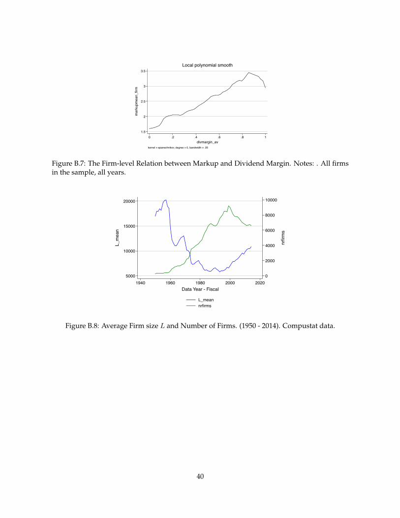
1.5

2

2.5

3

3.5

mar

kupm

ean_

firm

0 .2 .4 .6 .8 1divmargin_av

kernel = epanechnikov, degree = 0, bandwidth = .05

Local polynomial smooth

Figure B.7: The Firm-level Relation between Markup and Dividend Margin. Notes: . All firmsin the sample, all years.

0

2000

4000

6000

8000

10000

nrfir

ms

5000

10000

15000

20000

L_m

ean

1940 1960 1980 2000 2020Data Year - Fiscal

L_meannrfirms

Figure B.8: Average Firm size L and Number of Firms. (1950 - 2014). Compustat data.

.

40

0

5000

10000

15000

20000

1.2

1.3

1.4

1.5

1.6

1.7

Shar

e-w

eigh

ted

Mar

kup

(DLW

)

1960 1980 2000 2020Year

Share-weighted Markup (DLW)Nr M&AAverage value M&A (10,000 USD)

Figure B.9: Number and average value of M&A in the Compustat sample. (1950 - 2014).Notes. Compustat data.

.

41

References

ANTRAS, P. (2004): “Is the US aggregate production function Cobb-Douglas? New estimatesof the elasticity of substitution,” Contributions in Macroeconomics, 4(1).

ARMENTER, R. (2015): “A bit of a miracle no more: the decline of the labor share,” BusinessReview, Q3, 1–9.

ASKER, J., A. COLLARD-WEXLER, AND J. DE LOECKER (2017): “Market Power and Production(Mis)Allocation. A Study of the World Oil Market,” mimeo.

ASKER, J., J. FARRE-MENSA, AND A. LJUNGQVIST (2014): “Corporate investment and stockmarket listing: a puzzle?,” Review of Financial Studies.

AUTOR, D., D. DORN, L. F. KATZ, C. PATTERSON, AND J. VAN REENEN (2017): “The Fall ofthe Labor Share and the Rise of Superstar Firms,” Discussion paper, Centre for EconomicPerformance, LSE.

AUTOR, D. H., L. F. KATZ, AND M. S. KEARNEY (2008): “Trends in US wage inequality: Revis-ing the revisionists,” The Review of economics and statistics, 90(2), 300–323.

BAILY, M. N., AND B. P. BOSWORTH (2014): “US manufacturing: Understanding its past andits potential future,” The Journal of Economic Perspectives, 28(1), 3–25.

BAQAEE, D. R., AND E. FARHI (2017): “The Macroeconomic Impact of Microeconomic Shocks:Beyond Hulten’s Theorem,” Discussion paper, National Bureau of Economic Research.

BARKAI, S. (2017): “Declining Labor and Capital Shares,” Chicago Booth mimeo.BASU, S., AND J. G. FERNALD (1997): “Returns to scale in US production: Estimates and impli-

cations,” Journal of political economy, 105(2), 249–283.BERGER, D., AND J. VAVRA (2017): “Shocks vs. Responsiveness: What Drives Time-Varying

Dispersion?,” Discussion paper, National Bureau of Economic Research.BERNANKE, B. (2004): “The great moderation,” Washington, DC.BRESNAHAN, T. F. (1982): “The oligopoly solution concept is identified,” Economics Letters,

10(1-2), 87–92.(1989): “Empirical studies of industries with market power,” Handbook of industrial

organization, 2, 1011–1057.BRYNJOLFSSON, E. (1993): “The productivity paradox of information technology,” Communica-

tions of the ACM, 36(12), 66–77.BURDETT, K., AND K. L. JUDD (1983): “Equilibrium price dispersion,” Econometrica: Journal of

the Econometric Society, pp. 955–969.BURNSIDE, C. (1996): “Production function regressions, returns to scale, and externalities,”

Journal of monetary Economics, 37(2), 177–201.CABALLERO, R., E. FARHI, AND P.-O. GOURINCHAS (2017): “Accounting for Secular Trends in

Interest Rates, Returns on Capital, Earning Yields, and Factor Shares,” MIT mimeo.CAMPA, J. M., AND L. S. GOLDBERG (2005): “Exchange rate pass-through into import prices,”

Review of Economics and Statistics, 87(4), 679–690.COLLARD-WEXLER, A., AND J. DE LOECKER (2016): “Production Function Estimation with

Measurement Error in Inputs,” Discussion paper, National Bureau of Economic Research.

42

COOPER, R., AND J. EJARQUE (2003): “Financial frictions and investment: requiem in q,” Reviewof Economic Dynamics, 6(4), 710–728.

DAVIS, S. J., AND J. HALTIWANGER (2014): “Labor market fluidity and economic performance,”Discussion paper, National Bureau of Economic Research.

DAVIS, S. J., J. HALTIWANGER, R. JARMIN, AND J. MIRANDA (2007): “Volatility and dispersionin business growth rates: Publicly traded versus privately held firms,” in NBER Macroeco-nomics Annual 2006, Volume 21, pp. 107–180. MIT Press.

DAVIS, S. J., AND J. A. KAHN (2008): “Interpreting the great moderation: Changes in thevolatility of economic activity at the macro and micro levels,” The Journal of Economic Per-spectives, 22(4), 155–180.

DE LOECKER, J. (2011): “Product differentiation, multiproduct firms, and estimating the impactof trade liberalization on productivity,” Econometrica, 79(5), 1407–1451.

DE LOECKER, J., P. K. GOLDBERG, A. K. KHANDELWAL, AND N. PAVCNIK (2016): “Prices,Markups and Trade Reform,” Econometrica, 84(2).

DE LOECKER, J., AND P. T. SCOTT (2016): “Estimating market power Evidence from the USBrewing Industry,” Discussion paper, National Bureau of Economic Research.

DE LOECKER, J., AND F. M. P. WARZYNSKI (2012): “Markups and Firm-level Export Status,”American Economic Review, 102(6), 2437–2471.

DECKER, R., J. HALTIWANGER, R. JARMIN, AND J. MIRANDA (2014): “The secular decline inbusiness dynamism in the US,” University of Maryland mimeo.

EDMONDS, C., V. MIDRIGAN, AND Y. XU (2015): “Competition, Markups and the Gains fromInternational Trade,” The American Economic Review, 105, 3183–3221.

EECKHOUT, J., AND X. WENG (2017): “The Technological Origins of the Decline in Labor Mar-ket Dynamism,” mimeo.

ELSBY, M. W., B. HOBIJN, AND A. SAHIN (2013): “The decline of the US labor share,” BrookingsPapers on Economic Activity, 2013(2), 1–63.

FALLICK, B., C. FLEISCHMAN, AND J. PINGLE (2010): “The effect of population aging on theaggregate labor market,” in Labor in the New Economy, pp. 377–417. University of ChicagoPress.

GABAIX, X. (2011): “The granular origins of aggregate fluctuations,” Econometrica, 79(3), 733–772.

GABAIX, X., AND A. LANDIER (2008): “Why has CEO Pay Increased So Much?,” The QuarterlyJournal of Economics, 123(1), 49–100.

GANAPATI, S. (2016): “The Modern Wholesaler: Global Sourcing, Domestic Distribution, andScale Economies,” Yale mimeo.

GENESOVE, D., AND W. P. MULLIN (1998): “Testing static oligopoly models: conduct and costin the sugar industry, 1890-1914,” The RAND Journal of Economics, pp. 355–377.

GOLLIN, D. (2002): “Getting income shares right,” Journal of political Economy, 110(2), 458–474.GORDON, R. J. (2016): The rise and fall of American growth: The US standard of living since the civil

war. Princeton University Press.

43

GUVENEN, F., G. KAPLAN, J. SONG, AND J. WEIDNER (2017): “Lifetime Incomes in the UnitedStates over Six Decades,” Discussion paper, National Bureau of Economic Research.

HALL, R. (1988): “The Relation between Price and Marginal Cost in U.S. Industry,” Journal ofPolitical Economy, 96(5), 921–947.

HARBERGER, A. C. (1954): “Monopoly and Resource Allocation,” The American Economic Re-view, 44(2), 77–87.

HOPENHAYN, H. A. (1992): “Entry, exit, and firm dynamics in long run equilibrium,” Econo-metrica: Journal of the Econometric Society, pp. 1127–1150.

HYATT, H. R., AND J. R. SPLETZER (2013): “The recent decline in employment dynamics,” IZAJournal of Labor Economics, 2(1), 5.

JOVANOVIC, B. (1982): “Selection and the Evolution of Industry,” Econometrica, pp. 649–670.KAPLAN, G., AND S. SCHULHOFER-WOHL (2012): “Understanding the long-run decline in

interstate migration,” Discussion paper, National Bureau of Economic Research.KARABARBOUNIS, L., AND B. NEIMAN (2014): “The Global Decline of the Labor Share*.,” Quar-

terly Journal of Economics, 129(1).KARAHAN, F., B. PUGSLEY, AND A. SAHIN (2016): “Demographic Origins of the Startup

Deficit,” NY Fed mimeo.KELLER, W., AND S. YEAPLE (2009): “Multinational Enterprises, International Trade, and Pro-

ductivity Growth: Firm-Level Evidence from the United States,” Review of Economics andStatistics, 91(4), 821–831.

KOH, D., R. SANTAEULALIA-LLOPIS, AND Y. ZHENG (2017): “Labor Share Decline and Intel-lectual Property Products Capital,” Discussion paper, Washington University mimeo.

MELITZ, M. J., AND G. I. OTTAVIANO (2008): “Market size, trade, and productivity,” The reviewof economic studies, 75(1), 295–316.

OLLEY, G. S., AND A. PAKES (1996): “The Dynamics of Productivity in the TelecommunicationsEquipment Industry,” Econometrica: Journal of the Econometric Society, pp. 1263–1297.

SOLOW, R. M. (1987): “We’d better watch out,” New York Times Book Review, 36.YEH, C. (2017): “Are firm-level idiosyncratic shocks important for U.S. aggregate volatility?,”

University of Chicago.

44