The Rise of Market Power and the Macroeconomic Implications · The Rise of Market Power and the...

The Rise of Market Powerand the Macroeconomic Implications

Jan De Loecker1 Jan Eeckhout2

1Princeton and University of Leuven2University College London and UPF

NBER Summer Institute18 July, 2017

Motivation

• Several secular trends in last decades: wages, LF participation,labor share, labor mobility, migration rates, capital share,output growth slowdown

• Propose common cause: the rise in market power since 1980

• Little known about evolution & cross-section markup in macro

1. Data needed: long time series of firm-level data2. Estimation methods: demand approach uses model of

consumer behavior and competition

• This paper:

1. Document time-series and cross section of markup 1950-20142. Cost-based method; no inference from demand; mkt structure3. Illustrate how this can explain 7 secular trends since 1980

• We have nothing (little) to say about causes of change markup

MotivationSecular Increase since 1980: markup 1.18→ 1.67

1.1

1.2

1.3

1.4

1.5

1.6

1.7Sh

are

wei

ghte

d M

arku

p

1960 1970 1980 1990 2000 2010year

Figure: The Evolution of Average Markups (1950–2014), weighted

Data

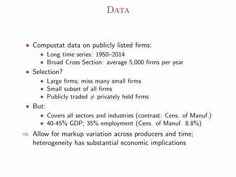
• Compustat data on publicly listed firms:• Long time series: 1950–2014• Broad Cross Section: average 5,000 firms per year

• Selection?• Large firms; miss many small firms• Small subset of all firms• Publicly traded 6= privately held firms

• But:• Covers all sectors and industries (contrast: Cens. of Manuf.)• 40-45% GDP; 35% employment (Cens. of Manuf. 8.8%)

⇒ Allow for markup variation across producers and time;heterogeneity has substantial economic implications

Producer Behavior

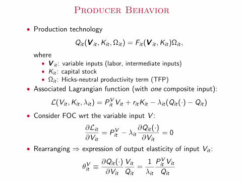
• Production technology

Qit(VVV it ,Kit ,Ωit) = Fit(VVV it ,Kit)Ωit ,

where• VVV it : variable inputs (labor, intermediate inputs)• Kit : capital stock• Ωit : Hicks-neutral productivity term (TFP)

• Associated Lagrangian function (with one composite input):

L(Vit ,Kit , λit) = PVit Vit + ritKit − λit(Qit(·)− Qit)

• Consider FOC wrt the variable input V :

∂Lit∂Vit

= PVit − λit

∂Qit(·)∂Vit

= 0

• Rearranging ⇒ expression of output elasticity of input Vit :

θVit ≡∂Qit(·)∂Vit

Vit

Qit=

1

λit

PVit Vit

Qit

Producer Behavior

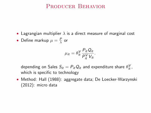
• Lagrangian multiplier λ is a direct measure of marginal cost

• Define markup µ = Pλ or

µit = θVitPitQit

PVit Vit

.

depending on Sales Sit = PitQit and expenditure share θVit ,which is specific to technology

• Method: Hall (1988): aggregate data; De Loecker-Warzynski(2012): micro data

Robustness

Benchmark Industry-Specific CD

1.1

1.2

1.3

1.4

1.5

1.6

1.7

Shar

e w

eigh

ted

Mar

kup

1960 1970 1980 1990 2000 2010year

1.1

1.2

1.3

1.4

1.5

1.6

1.7

1960 1970 1980 1990 2000 2010year

Share weighted Markup Markup (ind techn.)

Census Manufacturing Translog

1.1

1.2

1.3

1.4

1.5

1.6

1.7

1960 1970 1980 1990 2000 2010year

Share weighted Markup Share weighted markup (Manufacturing)

1.2

1.3

1.4

1.5

1.6

1.7

Shar

e w

eigh

ted

Mar

kup

1.5

2

2.5

Mar

kup

(ind

tech

n. T

rans

log)

1960 1970 1980 1990 2000 2010year

Markup (ind techn. Translog)Share weighted Markup

Cross-Sectional DecompositionHigher Markups for Smaller Firms

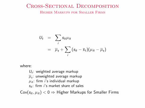
Ut =∑i

sitµit

= µt +∑i

(sit − st)(µit − µt)

where:

Ut : weighted average markupµt : unweighted average markupµit : firm i ’s individual markupsit : firm i ’s market share of sales

Cov(sit , µit) < 0⇒ Higher Markups for Smaller Firms

Cross-Sectional DecompositionHigher Markups for Smaller Firms

1

1.5

2

2.5

1960 1970 1980 1990 2000 2010year

Share weighted Markup mu_mean

Figure: Unweighted vs. Weighted Average Markup

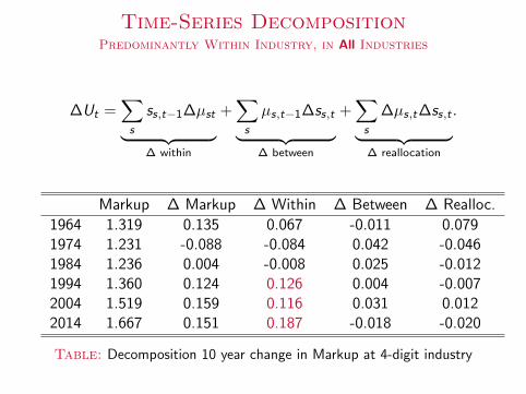
Time-Series DecompositionPredominantly Within Industry, in All Industries

∆Ut =∑s

ss,t−1∆µst︸︷︷︸∆ within

+∑s

µs,t−1∆ss,t︸︷︷︸∆ between

+∑s

∆µs,t∆ss,t︸︷︷︸∆ reallocation

.

Markup ∆ Markup ∆ Within ∆ Between ∆ Realloc.

1964 1.319 0.135 0.067 -0.011 0.0791974 1.231 -0.088 -0.084 0.042 -0.0461984 1.236 0.004 -0.008 0.025 -0.0121994 1.360 0.124 0.126 0.004 -0.0072004 1.519 0.159 0.116 0.031 0.0122014 1.667 0.151 0.187 -0.018 -0.020

Table: Decomposition 10 year change in Markup at 4-digit industry

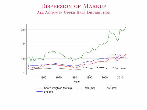
Dispersion of MarkupAll Action in Upper Half Distribution

1

1.5

2

2.5

1960 1970 1980 1990 2000 2010year

Share weighted Markup p90 (ms) p50 (ms)p75 (ms)

• Harberger (1954): roughly equally distributed profits; not now

Markup = Market Power?Dividends and Market Value

500000

1000000

1500000

2000000

Shar

e w

eigh

ted

Div

iden

d1.1

1.2

1.3

1.4

1.5

1.6

1.7

Mar

kup

1960 1970 1980 1990 2000 2010year

Markup Share weighted Dividend

0

2.00e+07

4.00e+07

6.00e+07

8.00e+07

Shar

e w

eigh

ted

Mar

ket V

alue

1.1

1.2

1.3

1.4

1.5

1.6

1.7

Mar

kup

1960 1970 1980 1990 2000 2010year

Markup Share weighted Market Value

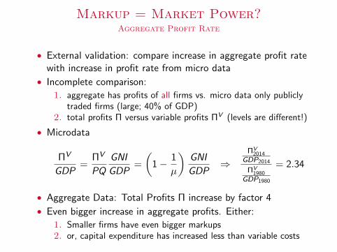
Markup = Market Power?Aggregate Profit Rate

• External validation: compare increase in aggregate profit ratewith increase in profit rate from micro data

• Incomplete comparison:

1. aggregate has profits of all firms vs. micro data only publiclytraded firms (large; 40% of GDP)

2. total profits Π versus variable profits ΠV (levels are different!)

• Microdata

ΠV

GDP=

ΠV

PQ

GNI

GDP=

(1− 1

µ

)GNI

GDP⇒

ΠV2014

GDP2014

ΠV1980

GDP1980

= 2.34

• Aggregate Data: Total Profits Π increase by factor 4

• Even bigger increase in aggregate profits. Either:

1. Smaller firms have even bigger markups2. or, capital expenditure has increased less than variable costs

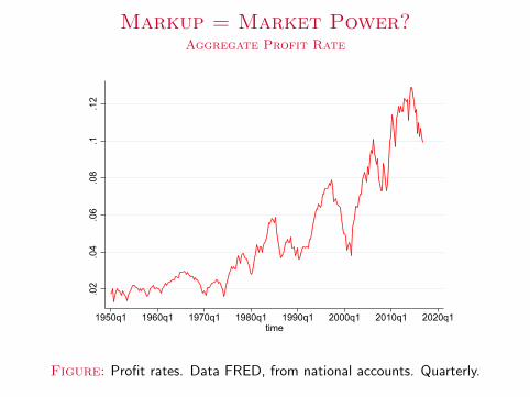
Markup = Market Power?Aggregate Profit Rate

.02

.04

.06

.08

.1.1

2

1950q1 1960q1 1970q1 1980q1 1990q1 2000q1 2010q1 2020q1time

Figure: Profit rates. Data FRED, from national accounts. Quarterly.

Summary of Facts

1. Sharp increase in Markup since 1980: 42%

2. High markup firms tend to be smaller

3. Only in the upper half of Markup distribution (espec. at top)

4. Mostly within industry (in all; no particular industries)

5. Markup = Market Power: total profits ×4

Macroeconomic Implications

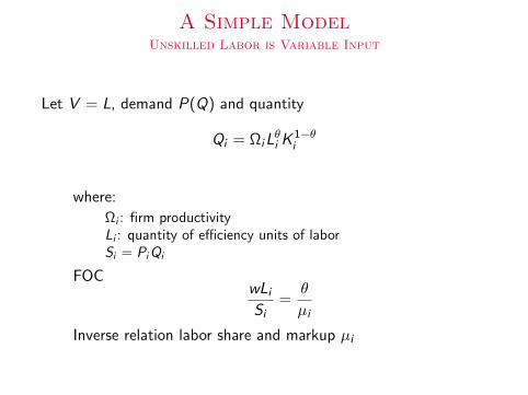
A Simple ModelUnskilled Labor is Variable Input

Let V = L, demand P(Q) and quantity

Qi = ΩiLθi K

1−θi

where:

Ωi : firm productivityLi : quantity of efficiency units of laborSi = PiQi

FOCwLiSi

=θ

µi

Inverse relation labor share and markup µi

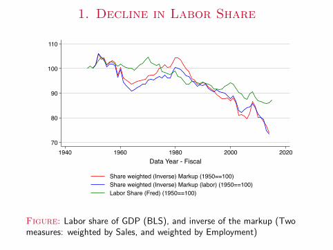
1. Decline in Labor Share

70

80

90

100

110

1940 1960 1980 2000 2020Data Year - Fiscal

Share weighted (Inverse) Markup (1950==100) Share weighted (Inverse) Markup (labor) (1950==100) Labor Share (Fred) (1950==100)

Figure: Labor share of GDP (BLS), and inverse of the markup (Twomeasures: weighted by Sales, and weighted by Employment)

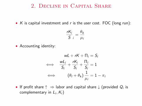
2. Decline in Capital Share

• K is capital investment and r is the user cost. FOC (long run):

rKi

S i=θkµi

• Accounting identity:

wL + rK + Πi = Si

⇐⇒ wLiSi

+rKi

Si+

Πi

Si= 1

⇐⇒ (θl + θk)1

µi= 1− πi

• If profit share ↑ ⇒ labor and capital share ↓ (provided Qi iscomplementary in Li ,Ki )

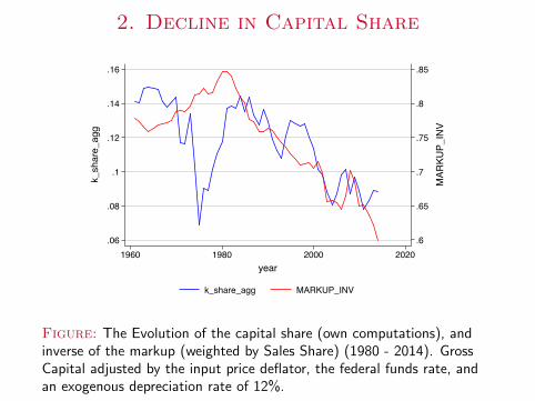
2. Decline in Capital Share

.6

.65

.7

.75

.8

.85

MAR

KUP_INV

.06

.08

.1

.12

.14

.16

k_share_agg

1960 1980 2000 2020year

k_share_agg MARKUP_INV

Figure: The Evolution of the capital share (own computations), andinverse of the markup (weighted by Sales Share) (1980 - 2014). GrossCapital adjusted by the input price deflator, the federal funds rate, andan exogenous depreciation rate of 12%.

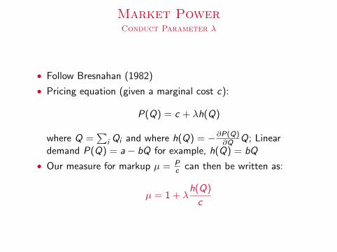
Market PowerConduct Parameter λ

• Follow Bresnahan (1982)

• Pricing equation (given a marginal cost c):

P(Q) = c + λh(Q)

where Q =∑

i Qi and where h(Q) = −∂P(Q)∂Q Q; Linear

demand P(Q) = a− bQ for example, h(Q) = bQ

• Our measure for markup µ = Pc can then be written as:

µ = 1 + λh(Q)

c

Market Power

• Market power can change with technology, externalities,network goods, entry barriers, preferences (Dixit-Stiglitz),market structure, consumer behavior (Burdett-Judd),...

• Our model: change in λ = Cournot

1. Market power changes exogenously with λ2. Number of firms per market N = 1

λ3. In a given market, all N firms have same technology Ωi

4. Linear Demand, to capture incomplete pass-through ( 6= CES)

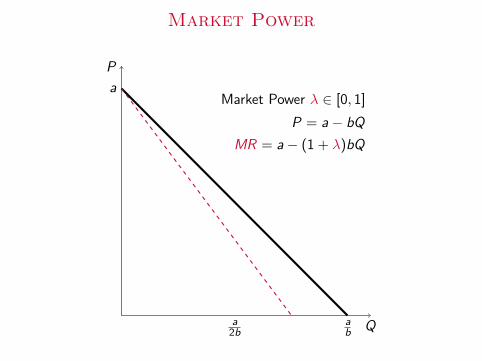
Market Power

Q

P

ab

a2b

aMarket Power λ ∈ [0, 1]

P = a− bQ

MR = a− (1 + λ)bQ

Market Power

Q

P

ab

a2b

aMonopoly

Market Power λ = 1

P = a− bQ

MR = a− 2bQ

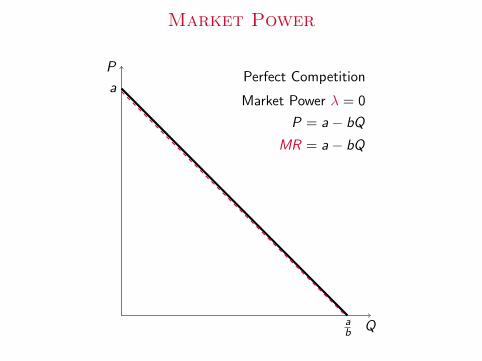
Market Power

Q

P

ab

aPerfect Competition

Market Power λ = 0

P = a− bQ

MR = a− bQ

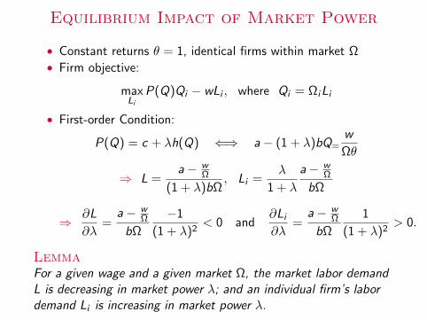
Equilibrium Impact of Market Power

• Constant returns θ = 1, identical firms within market Ω• Firm objective:

maxLi

P(Q)Qi − wLi , where Qi = ΩiLi

• First-order Condition:

P(Q) = c + λh(Q) ⇐⇒ a− (1 + λ)bQ=w

Ωθ

⇒ L =a− w

Ω

(1 + λ)bΩ, Li =

λ

1 + λ

a− wΩ

bΩ

⇒ ∂L

∂λ=

a− wΩ

bΩ

−1

(1 + λ)2< 0 and

∂Li∂λ

=a− w

Ω

bΩ

1

(1 + λ)2> 0.

LemmaFor a given wage and a given market Ω, the market labor demandL is decreasing in market power λ; and an individual firm’s labordemand Li is increasing in market power λ.

Compustat DataFirm Size and Number of Firms

0

2000

4000

6000

8000

10000

nrfir

ms

5000

10000

15000

20000

L_m

ean

1940 1960 1980 2000 2020Data Year - Fiscal

L_meannrfirms


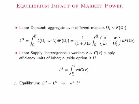
• Labor Demand: aggregate over different markets Ωi ∼ F (Ωi )

LD =

∫ Ω

ΩL(Ωi ;w ;λ)dF (Ωi ) =

1

(1 + λ)b

∫ Ω

Ω

(a

Ωi− w

Ω2i

)dF (Ωi )

• Labor Supply: heterogeneous workers z ∼ G (z) supplyefficiency units of labor; outside option is U

LS =

∫ 1

Uw

zdG (z)

∴ Equilibrium: LD = LS ⇒ w?, L?


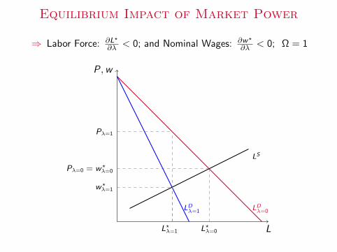
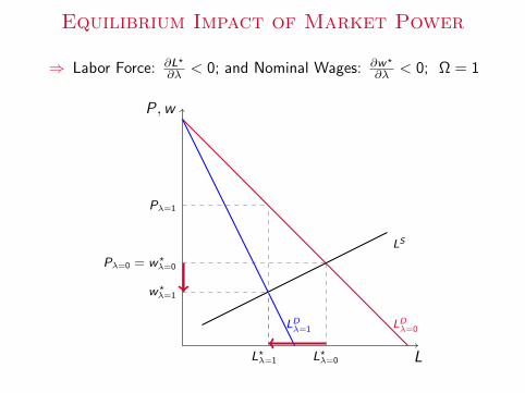
⇒ Labor Force: ∂L?

∂λ < 0; and Nominal Wages: ∂w?

∂λ < 0; Ω = 1

L

P,w

LDλ=0

LS

Pλ=0 = w?λ=0

L?λ=0

LDλ=1

w?λ=1

Pλ=1

L?λ=1

3. Decline in (Low Skill) WagesEvidence

• Without Growth: nominal wages decline

• With Growth: nominal wages relative to GDP decline

• Double Impact since 1980:

1. Nominal wages ↓2. P ↑ 42%: real wages w

P ↓ further relative to perf. comp.

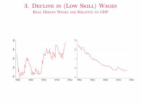
3. Decline in (Low Skill) WagesReal Median Wages and Relative to GDP

310

320

330

340

350

1980q1 1990q1 2000q1 2010q1 2020q1

.6.8

11.

21.

4

1980q1 1990q1 2000q1 2010q1 2020q1

4. Decline in Labor Force ParticipationEvidence

.58

.6.6

2.6

4.6

6.6

8

1950m1 1960m1 1970m1 1980m1 1990m1 2000m1 2010m1 2020m1time

Notes. From CPS.

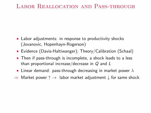
Labor Reallocation and Pass-through

• Labor adjustments: in response to productivity shocks(Jovanovic, Hopenhayn-Rogerson)

• Evidence (Davis-Haltiwanger); Theory/Calibration (Schaal)

• Then if pass-through is incomplete, a shock leads to a lessthan proportional increase/decrease in Q and L

• Linear demand: pass-through decreasing in market power λ

⇒ Market power ↑ → labor market adjustment ↓ for same shock

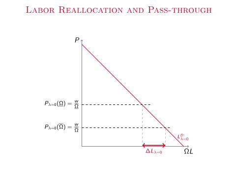
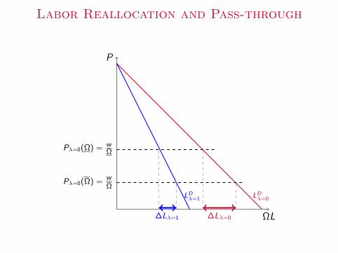
Labor Reallocation and Pass-through

ΩL

P

LDλ=0

∆Lλ=0

wΩ

wΩ

Pλ=0(Ω) =

Pλ=0(Ω) =

LDλ=1

∆Lλ=1

Pλ=1(Ω)

Pλ=1(Ω)

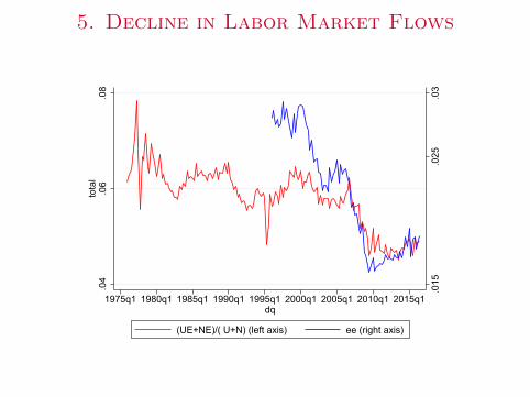
5. Decline in Labor Market Flows

.015

.025

.03

.04

.06

.08

tota

l

1975q1 1980q1 1985q1 1990q1 1995q1 2000q1 2005q1 2010q1 2015q1dq

(UE+NE)/( U+N) (left axis) ee (right axis)

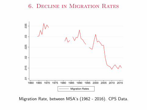
6. Decline in Migration Rates

.01

.015

.02

.025

.03

.035

1960 1965 1970 1975 1980 1985 1990 1995 2000 2005 2010 2015

Migration Rates

Migration Rate, between MSA’s (1962 - 2016). CPS Data.

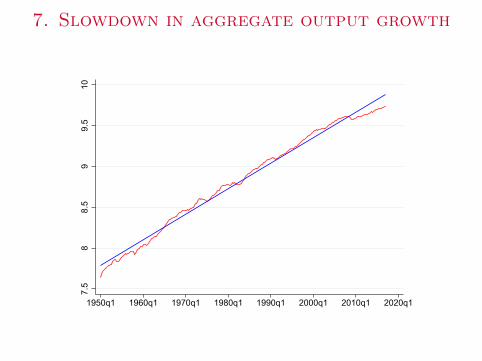
7. Slowdown in aggregate output growth

7.5

88.

59

9.5

10

1950q1 1960q1 1970q1 1980q1 1990q1 2000q1 2010q1 2020q1

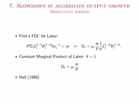
7. Slowdown in aggregate output growthProductivity Growth

• Firm’s FOC for Labor:

PΩiLθ−1i K 1−θ

i θµ−1i = w ⇒ Ωi = µi

w

P

1

θL1−θi K 1−θ

i .

• Constant Marginal Product of Labor: θ = 1

Ωi = µiw

P

• Hall (1988)

7. Slowdown in aggregate output growthProductivity Growth

-.1

-.05

0

.05

.1

1960 1980 2000 2020

omega_gamma_gr TFP_gamma_grlpoly smooth: omega_gamma_gr lpoly smooth: TFP_gamma_gr

-.04

-.02

0

.02

.04

.06

wed

ge

1960 1980 2000 2020Data Year - Fiscal

90% CI wedge lpoly smooth

Conclusions

1. Sharp rise in Market Power since 1980

2. Significant macroeconomic implications: 7 secular trends

ConclusionsOpen Questions

1. Causes? Technology, M&A,...

2. Other secular trends?

1. decrease in startup rate of new firms2. decrease long term interest rate: capital D ↓, S ↑3. increase in wage inequality: profit sharing managers4. the great moderation...

3. Two (uncomfortable) Consequences – Food for Thought

1. Inflation is too high: 42% increase price level; 1% per year⇒ Policy: anti-trust, not Federal Reserve!

2. Stock market over-valued (compared to Perfect Competition)⇒ Stock market increase 6= economic growth

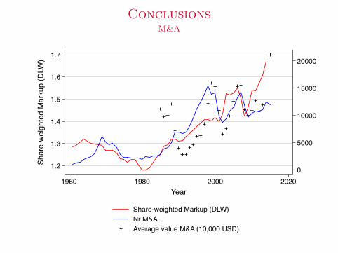
ConclusionsM&A

0

5000

10000

15000

20000

1.2

1.3

1.4

1.5

1.6

1.7

Shar

e-w

eigh

ted

Mar

kup

(DLW

)

1960 1980 2000 2020Year

Share-weighted Markup (DLW)Nr M&AAverage value M&A (10,000 USD)

ConclusionsGreat Moderation

-50

510

15

1950q1 1960q1 1970q1 1980q1 1990q1 2000q1 2010q1 2020q1time

ConclusionsStock Market Valuation

0

5000

10000

15000

20000

DOW

JO

NES

(Defl

ated

CPI

)

1.2

1.3

1.4

1.5

1.6

1.7

Shar

e we

ight

ed M

arku

p

1960 1970 1980 1990 2000 2010year

Share weighted MarkupDOW JONES (Deflated CPI)


1. Causes of Market Power? Technology, M&A,...






Whenever a theory appears to you as the only possibleone, take this as a sign that you have neither understoodthe theory nor the problem which it was intended to solve

Karl Popper

The Rise of Market Powerand the Macroeconomic Implications

Jan De Loecker1 Jan Eeckhout2

1Princeton and University of Leuven2University College London and UPF

NBER Summer Institute18 July, 2017

Causes?

• Production Technology:• Big Retail vs. manufacturing and services• Network goods

• Finance:• Mergers and Acquisitions• Cross-ownership of competitors• Private Equity – under the radar• Vertical Integration

• Preferences:• Price Differentiation improved through technology• Brand dependence

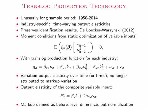
Translog Production Technology

• Unusually long sample period: 1950-2014

• Industry-specific, time-varying output elasticities

• Preserves identification results, De Loecker-Warzynski (2012)

• Moment conditions from static optimization of variable inputs:

E(ξit(βββ)

[vit−1

v2it−1

])= 0,

• With translog production function for each industry:

qit = βv1vit + βk1kit + βv2v2it + βk2k

2it + ωit + εit

• Variation output elasticity over time (or firms), no longerattributed to markup variation

• Output elasticity of the composite variable input:

θvit = βv1 + 2βv2vit

• Markup defined as before; level difference, but normalization

Cross-Sectional DecompositionAcross All Industries

1.2

1.3

1.4

1.5

1.6

1.7

1940 1960 1980 2000 2020year

Markup Mean 4digit

Figure: Industry disaggregation

Markup = Market Power?Dividends

• Individual firm level: firm-level average markup (all years) andthe share of total dividends in total sales

1.5

2

2.5

3

3.5

mar

kupm

ean_

firm

0 .2 .4 .6 .8 1divmargin_av

kernel = epanechnikov, degree = 0, bandwidth = .05

Local polynomial smooth

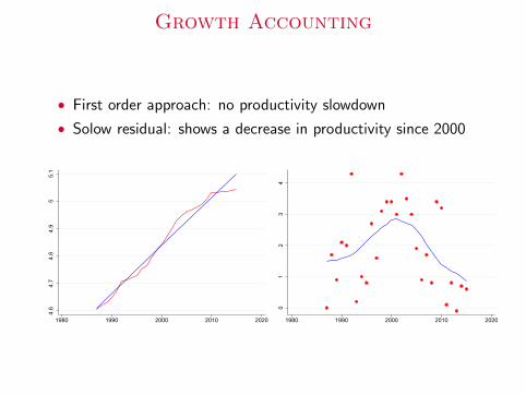
Growth Accounting

• First order approach: no productivity slowdown

• Solow residual: shows a decrease in productivity since 2000

4.6

4.7

4.8

4.9

55.

1

1980 1990 2000 2010 2020

01

23

4

1980 1990 2000 2010 2020

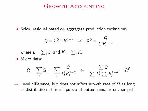
Growth Accounting

• Solow residual based on aggregate production technology

Q = ΩSLθK 1−θ ⇒ ΩS =Q

LθK 1−θ

where L =∑

i Li and K =∑

i Ki

• Micro data:

Ω =∑i

Ωi =∑i

Qi

Lθi K1−θi

↔∑

Qi∑i Lθi

∑i K

1−θi

= ΩS

→ Level difference, but does not affect growth rate of Ω as longas distribution of firm inputs and output remains unchanged

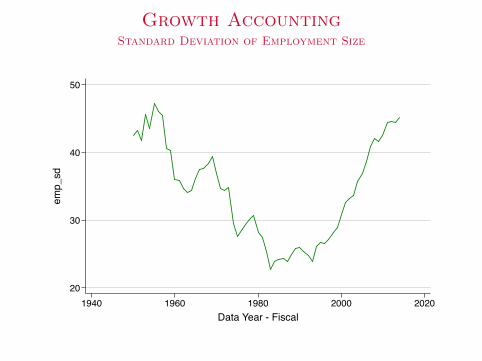
Growth AccountingStandard Deviation of Employment Size

20

30

40

50

emp_

sd

1940 1960 1980 2000 2020Data Year - Fiscal

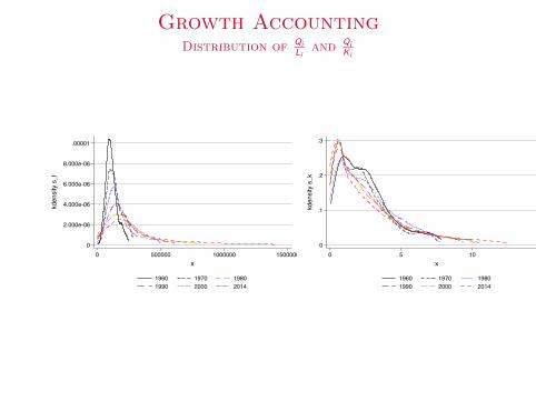
Growth AccountingDistribution of Qi

Liand Qi

Ki

0

2.000e-06

4.000e-06

6.000e-06

8.000e-06

.00001

kden

sity

s_l

0 500000 1000000 1500000x

1960 1970 19801990 2000 2014

0

.1

.2

.3

kden

sity

s_k

0 5 10 15x

1960 1970 19801990 2000 2014

Growth AccountingDistribution of Qi

Lθi K1−θi

0

.0001

.0002

.0003

.0004

kden

sity

s_l

k

0 5000 10000 15000 20000 25000x

1960 1970 19801990 2000 2014

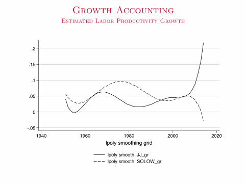
Growth AccountingEstimated Labor Productivity Growth

-.05

0

.05

.1

.15

.2

1940 1960 1980 2000 2020lpoly smoothing grid

lpoly smooth: JJ_grlpoly smooth: SOLOW_gr

The Rise of Market Power and the Macroeconomic Implications · The Rise of Market Power and the...

Documents

Transcript of The Rise of Market Power and the Macroeconomic Implications · The Rise of Market Power and the...