The Rise of ETF Trading and the Bifurcationof Liquidity∗

Jonathan BrogaardDavid Eccles School of Business

University of Utah

Davidson HeathDavid Eccles School of Business

University of Utah

Da HuangDavid Eccles School of Business

University of Utah

November 14, 2019

.

∗We thank Rajesh Aggarwal and Matt Ringgenberg for comments. We thank Shaun Davies for sharingcode and data. Email: davidson.heath@eccles.utah.edu.

.

The Rise of ETF Trading and the Bifurcation of Liquidity

Abstract

In the last two decades the assets under management of passively managed exchange traded

funds (ETFs) has risen dramatically. At the same time liquid stocks have become more

liquid while illiquid stocks have not experienced a similar improvement. We model investors

shifting from trading individual stocks to trading ETFs and generate predictions consistent

with the documented bifurcation in liquidity. Using daily ETF creation and redemption

activity, we provide empirical evidence that closely matches the model’s predictions. The

results show that the effects of ETFs on underlying asset markets are driven by their index

replication strategy.

JEL: G11, G12, G20

In recent years the structure of U.S. equities has changed dramatically. In 1998 there was

$2 billion of assets under management (AUM) in exchange traded funds (ETFs); in 2018

the total AUM of U.S. equity ETFs was over $3.5 trillion. In terms of trading volume ETFs

went from near zero to accounting for 32% in two decades. During this same period of time

the U.S. stock market has become more liquid (Angel, Harris, & Spatt, 2015). However, the

improvement in liquidity has not been uniform: liquid stocks have become more liquid while

illiquid stocks have not experienced such gains.1 Figure 1 shows how the liquidity of U.S.

equities has evolved since 2000. In this paper we examine whether the rise of ETF trading

can help explain the recent bifurcation of liquidity in U.S. equity markets.

Insert Figure 1 About Here

We develop a theoretical model that suggests that ETF trading may have a differential

effect on asset liquidity. Two key features of ETFs produce this differential effect. First,

ETFs are a substitute for trading individual stocks. Investors will transfer their trading

activity from individual stocks to a single ETF that represents those holdings. The second

feature is that ETFs that passively track an index can, and frequently do, deviate from the

precise weights of the index. The trading activity of the investors is not simply substituted

one for one by the ETF but is tilted towards the stocks the ETF chooses to sample. Based

on these two features we generate a number of predictions that follow from investors mi-

grating from investing in individual stocks to ETFs. The model predicts that ETFs will

systematically underweight or omit index assets that are less liquid ex ante. Consequently

there will be a bifurcation in stock liquidity as noise trading flows preferentially into more

liquid index members.

1Hendershott, Jones, and Menkveld (2011); Jones (2013); Haslag and Ringgenberg (2016).

1

Empirically we find that both predictions are borne out in the data. ETFs are more

likely to omit less liquid index stocks from their holdings, and ETF primary flows have a

differential effect on stock liquidity. As the magnitude of ETF primary flow increases – in

either direction – liquid stocks become more liquid, while illiquid stocks become less liquid.

This effect is separate from the documented effects of market fragmentation and algorithmic

trading.

Although straightforward in principle, replicating a target index entails nontrivial prob-

lems of implementation. Models of index investing often assume that index funds simply

mirror the weights of their target index. In practice ETFs have considerable discretion in

defining their creation / redemption basket (Lettau & Madhavan, 2018) and many ETF

redemption baskets diverge from the weights of their target index. Six of the ten largest

ETFs as of 2018 state in their prospectus that they statistically replicate their target index

by investing in a basket of representative securities.2

We model the fundamental tradeoff faced by index funds: To simultaneously minimize

expected tracking error and expected transactions costs. The model applies to both ETFs

(that set the creation and redemption basket for authorized participants) and traditional

open-ended index funds (that rebalance their portfolio after inflows and outflows). For fund

holdings the model predicts that index assets’ optimal weighting is driven by their transaction

costs, volatility, and correlation with other index assets. The more expensive to trade and

the less correlated with the index the more likely the asset will be underweighted or omitted.

2One example is the Vanguard Total Stock Market ETF (VTI), the third largest ETF by assets as of2018. The fund’s prospectus states, “The Fund invests by sampling the Index, meaning that it holds abroadly diversified collection of securities that, in the aggregate, approximates the full Index in terms ofkey characteristics.” Sampling or “optimized” index replication is not only popular with funds that trackrelatively illiquid indexes, but is also used by ETFs that track highly liquid indexes. For example, the secondlargest ETF as of 2018, the iShares Core S&P 500 ETF (IVV), states in its prospectus that BlackRock “usesa representative index sampling strategy to manage the Fund.”

2

We examine these predictions and find support for them in the fund holdings data.

We next turn to the effects of ETF trading on underlying asset markets. The most

important prediction of the model is that ETF trading activity due to primary flows (i.e. the

creation and redemption of ETF shares in exchange for the posted basket of index assets)

amplifies preexisting differences in liquidity as less liquid index assets are systematically

underweighted or omitted in the ETF’s basket. The fund’s replication strategy moves noise

trading out of illiquid index assets and into liquid index assets. We test these predictions

and find support for them in the stock-level daily data. On days when ETF primary flow is

higher, both positively and negatively, we find that liquidity is higher for index stocks that

are more liquid ex ante and lower for index stocks that are illiquid ex ante.

A unique prediction of the model is that the effects on index asset liquidity should be

different for ETFs that follow a sampling strategy compared to ETFs that follow a full

replication strategy. We test this prediction by exploiting the fact that investors and traders

are indifferent whether a given ETF is a sampler or a full replicator. We find that the

bifurcation in stock liquidity is driven entirely by primary flows in sampling ETFs.

Unobserved variables such as the arrival of market-moving news could also drive ETF

primary flows and asset liquidity at the same time. We address this concern in two ways.

First, we explicitly add daily market movements as a competing factor; second, we restrict

the sample to only include days when market-moving news does not arrive. The differential

effects of ETF activity on asset liquidity are larger, inconsistent with market-wide news

driving our results.

Finally, the rise of ETFs is not the only possible explanation for the differential liquidity

effects across the U.S. stock market in recent years. Two alternative explanations are often

mentioned: fragmentation and algorithmic trading. Regulation National Market System

3

(Reg NMS) was established in 2005 and had significant effects on quoted spreads, market

fragmentation, and market quality that differ by stock market capitalization (Haslag &

Ringgenberg, 2016). Algorithmic and high frequency trading have risen significantly for a

segment of the stock market (Weller, 2017). We find that measures of market fragmentation

and algorithmic trading activity do not explain the differential effects of ETF activity on

asset liquidity.

The findings are consistent with the hypothesis that the effects of ETFs on underlying

asset markets depend on their index replication strategy. This paper makes contributions to

both theoretical and empirical research on passive investing. Theoretical studies of passive

investing assume that passive funds replicate the weights of their benchmark index pro rata.

But this is not the case. Our results demonstrate that models of the impact of passive

investing on asset prices can be made richer and more realistic by taking into account the

replication strategy of passive funds. Moreover, empirical studies of passive investing often

implicitly take full replication as given by using index assignment to study the treatment

effects of index investing. Our results show that as a result the effects of index investing on

the underlying assets may be mismeasured.

This paper focuses on two strands of the literature. First, a large literature has investi-

gated the growth of passive and ETF investing and its effects on individual stocks and firms.

Greenwood (2007) finds that a higher index weight leads a stock to co-move more with the in-

dex and less with stocks that are not in the index. The finding is supported by Da and Shive

(2018), who attribute the increased co-movement to ETF arbitrage activity. Ben-David,

Franzoni, and Moussawi (2018) find that increased ETF ownership leads to higher stock

volatility, due to arbitrage trading between ETFs’ market price and net asset value (NAV).

Israeli, Lee, and Sridharan (2017) find that increased ETF ownership leads to lower price

4

efficiency, higher return synchronicity, and lower analyst coverage of the securities in the

underlying basket. Evans, Moussawi, Pagano, and Sedunov (2019) find that increased ETF

ownership increases the intraday bid-ask spreads of the underlying stocks. Saglam, Tuzun,

and Wermers (2019) find that increased ETF ownership makes the underlying stock in the

indexes more liquid. Agarwal, Hanouna, Moussawi, and Stahel (2018) find that increased

ETF ownership increases the commonality in liquidity of the underlying stocks.

We add to the literature by focusing on the implications of the infrastructure used in ETF

trading. ETFs often sample a subset of liquid index assets, and underweight or omit less

liquid index assets. We show that this replication strategy amplifies preexisting differences

in asset liquidity: Liquid assets become more liquid, while illiquid assets become less liquid.

We explicitly examine the create/redeem mechanism as the primary channel through which

ETFs affect the underlying index assets, and the implications for the liquidity of underlying

index assets.

Second, this paper relates to theoretical work on ETFs. We construct a model of optimal

index replication and show how index replication strategy determines the effects of ETF

trading on underlying asset markets.Carpenter (2000) and Basak, Pavlova, and Shapiro

(2007) show that fund flows tilt the portfolio toward stock that belong to the benchmark

because of fund managers’ risk aversion. Malamud (2016) constructs a general equilibrium

model in which ETF creation/redemption serves as a shock propagation mechanism; Pan

and Zeng (2019) construct a model in which a liquid ETF tracks a single illiquid asset, and

they analyze the effects of authorized participants’ market making activity on the asset’s

liquidity. These models assume the ETF basket replicates the underlying index. By contrast

we show that create/redeem activity tilt the ETF portfolio toward more liquid stocks within

its benchmark as ETF providers jointly minimize the trading cost and tracking error.We

5

characterize the optimal strategic differences between the basket and the index and the

resulting differential effects on asset markets.

I. Model

We construct a simple one-period model that captures the fundamental tradeoff faced by

all passively managed index funds: To simultaneously minimize expected tracking error and

expected transaction costs. The model is written from the point of view of an ETF provider;

we show in Appendix B that the same decision problem and solution applies to traditional

open-ended index funds as well.

A. Setup

There are N assets in the market with a vector of prices p, and one-period excess returns r

which are normally distributed with expectation 0 and covariance matrix Σ.

There are three types of agent: ETF providers, authorized participants, and investors.

We consider the market for ETFs that track a specified index such as the S&P 500 or the

Russell 2000 or the CRSP value-weighted equity index. The index is a vector of weights v

that add to 1 and are exogenous and fixed.3

An ETF provider enters the market by publishing a basket, which is a vector of weights

w that add to 1. She agrees to create or redeem shares of the ETF in exchange for that

basket of individual assets.4 The net asset value (NAV) of ETF shares is NAV = w′p.

3We do not consider the complexities introduced when a fund specifies its own index, as is apparentlycommon among smaller niche funds (Robertson, 2019). While numerous, such funds represent a tiny fractionof ETF trading volume.

4Some ETF providers also allow the authorized participants to create or redeem ETF shares in exchangefor cash. After netting the daily primary flow from its authorized participants, the provider may transact inderivatives or the underlying asset markets to zero out its residual position. As long as the ETF provider

6

The provider incurs administrative costs and collects a management fee, both of which are

proportional to its assets under management. There is free entry, so in equilibrium ETF

providers’ fees equal their costs.

The ETF provider also nominates one or more authorized participants (APs) who have

access to the creation and redemption mechanism. The AP continuously posts bid and offer

prices for one ETF share. When he gets lifted (hit), he immediately buys (sells) the basket

of underlying assets w. In so doing, he incurs a transaction cost C(w). He then immediately

exchanges the basket for one ETF share.

The AP never bears any risk, and simply makes the market for ETF shares by carrying

out the arbitrage with the basket of individual assets. Thus, the bid and offer prices that

the AP posts are pinned down by the transaction costs. Specifically, the AP’s profit from

posting the offer NAV + b and being lifted is:

= (NAV + b)− (w′p + C(w))

= b− C(w)

As long as the provider nominates at least two APs, if one posts an offer that is above

the zero-profit bound, the other will undercut them. That is, competition between APs is

Bertrand. Thus, the bid and offer prices that investors face to trade the ETF shares are

NAV ± C(w).

There is a unit mass of atomistic investors. In the competition between ETFs, all investors

prefer an ETF that has a lower bid/ask spread and a lower tracking error. The expected

faces nonzero transaction costs of doing so, the model is the same.

7

squared tracking error of the ETF is

E[(wr − vr)2] = (w − v)′Σ(w − v)

Thus, in equilibrium the ETF that captures the market is the one that minimizes

U = C(w) + λ(w − v)′Σ(w − v)

where λ is the shadow price that investors attach to a higher tracking error (term 2)

relative to a higher bid/ask spread (term 1).5

B. Fund Weights

The first order condition for the optimal weight of the fund in asset i is:

0 =∂C

∂wi

+ 2λ∑j

(wj − vj)σiσjρij

Cov(ri, rETF − rIndex)

∂C/∂wi

= −1/2λ

That is, the optimality condition for each asset is that the marginal increase in trading

5We assume that all investors have the same preference λ. Relaxing this assumption would result in a“frontier” of ETFs that express different tradeoffs between tracking error and transaction costs and caterto investors with different preferences. In practice, the multiplicity of funds tracking the same index seemsto be driven by investor search costs and not by different investor preferences (Hortacsu & Syverson, 2004).Appendix B shows that the same decision problem and solution applies to traditional open-ended indexfunds as well.

8

costs equals the marginal decrease in the expected tracking error, which is a product of the

covariance of ri with the fund’s total tracking error.

To solve for w explicitly, we specify the trading cost as quadratic and additively separa-

ble:6

C(w) =∑i

ciw2i

where ci measures the the trading cost of stock i.

It follows that:

0 = 2ciwi + 2λwiσ2i − 2λviσ

2i + 2λ

∑j 6=i

(wj − vj)σiσjρij

w∗i =

(1

1 + ci/λσ2i

)vi +

(1

1 + ci/λσ2i

)∑j 6=i

(vj − wj)βj,i (1)

Intuitively, the first term says that in general, index holdings are underweighted relative

to their index weight vi. The optimal weight balances transaction costs against the direct

contribution to tracking error (hence, ci over λσ2i ). The second term captures the indirect

second-order effects on tracking error: An asset that covaries positively with other index

constituents that are underweighted has a higher optimal weight, and vice versa.

In general we expect the first term, which captures the direct effects on trading costs

and tracking error, to dominate. However, there are exceptions, such as index futures and

6Almgren, Thum, Hauptmann, and Li (2005) propose that trading cost is exponential in order size foreach asset, and using a large set of execution data they estimate the exponent to be 1.375. Our quadraticcost function yields the same predictions in simple closed form.

9

redundant (highly correlated) assets. Appendix B analyzes these cases in detail.

The model predicts that the optimal weight w∗i is

• Decreasing in ci, as

∂w∗i∂ci

= − 1

(1 + ci/λσ2i )2

(vi +

∑j 6=i

(vj − wj)βj,i

)< 0

because in general vi > wi. This means a more illiquid stock has a lower optimal weight

in the basket.

• Increasing in ρij, as

∂w∗i∂ρij

=1

1 + ci/λσ2i

(vj − wj)σiσj > 0

because again, in general vi > wi. This means when the stock has higher correlation

with other index assets, its optimal weight is higher.

• Ambiguous in σi, as

∂w∗i∂σi

=2λciσi

(λσ2i + ci)2

vi +λ(ci − λσ2

i )

(λσ2i + ci)2

∑j 6=i

(vj − wj)σjρij

can be either positive or negative. The first term is always positive: the second term

may be positive or negative.

C. Asset Liquidity

Our model predicts that ETFs, and passive index funds in general, are more likely to omit

index assets with relatively 1) high trading costs, 2) low correlation with the index, and 3)

10

high volatility. Next we explore the effects of ETF trading on underlying asset markets.

Consider two index assets that are identical except for their liquidity: The market for

A is relatively liquid while the market for B is relatively illiquid, i.e. the price impact of

trading cA < cB. In the Kyle (1985) equilibrium, this means

βA =1

2

σAf

σAz

< βB =1

2

σBf

σBz

We model the difference in liquidity as more noise traders participating in the market for

asset A, i.e. σAz > σB

z . When an index ETF is introduced to the market, the noise traders

who previously traded in both assets (“homemade indexing”) migrate out of the individual

asset markets into the ETF market because the ETF is cheaper to trade.

Because assets A and B have the same index weight, the same portion δ ∈ (0, 1) of noisy

traders move out of both individual asset markets. This causes both assets’ liquidity to fall:

β′

A =1

2

σfσAz (1− δ)

> βA

β′

B =1

2

σfσBz (1− δ)

> βB

At the same time, as they move to trading the ETF instead, whose creation/redemption

basket includes A but omits B,7 authorized participants will trade asset A on behalf of the

noise traders. The trading volume generated by APs is still noise trading, as the APs simply

serve as a conduit for execution. Let κ > 0 be the additional noisy volume generated by APs.

7We focus on the case in which asset B is omitted, but the predictions are qualitatively the same if assetB is included but underweighted.

11

Then the overall effect of the introduction of the ETF on the individual assets’ liquidity is

β′′

A =1

2

σfσAz (1− δ)(1 + κ)

β′′

B =1

2

σfσBz (1− δ)

Thus, the liquidity of asset B becomes worse (price impact of trading is larger). For asset

A, if the ETF’s low trading cost attracts additional volume into the ETF market so that

(1 +κ)(1− δ) > 1, asset A becomes more liquid. Otherwise, the liquidity of asset A can stay

the same or become worse.

Regardless, our model predicts an unambiguous decline of the liquidity of asset B relative

to asset A:

(β′′

B − β′′

A)− (βB − βA) =σf2

((

1

σBz (1− δ)

− 1

σAz (1− δ)(1 + κ)

)− (1

σBz

− 1

σAz

)

)> 0

Thus, because of the ETF provider’s optimal underweighting or omission of illiquid assets

when they form the creation/redemption basket, the introduction of the ETF creates a

“Matthew Effect” – an effect that amplifies pre-existing inequality – in the liquidity of index

assets. Liquid assets become relatively more liquid, while illiquid assets become relatively

less liquid.

12

II. Data

Our holdings data covers all stocks in the Russell 3000 index from 2009 to 2018. Thus, we

exclude (as the Russell 3000 does) micro-cap and foreign stocks. We obtain quarterly fund

holdings from the union of the CRSP mutual fund holdings database and the Thompson-

Reuters S12 database, as both databases have gaps in their coverage. Returns, trading

volume and other market data for both stocks and ETFs are from the CRSP monthly file.

We use index membership and weights by month, directly from Russell Investments, for the

Russell 1000 (large-cap) and Russell 2000 (small-cap) indexes.

Table 1 Panel A shows that our sample stocks, the monthly Russell 3000 list from 2006

to 2018, are a representative majority of large, mid and small-cap U.S. listed stocks. Note

that the Russell 3000 index (and thus our sample) excludes very small micro-cap stocks.

Insert Table 1 About Here

Table 1 Panel B shows summary statistics for the ETFs in our sample, which is all U.S.

equity ETFs from 2006 to 2018 in the CRSP mutual funds database with at least $10 million

in assets under management. Figure 2 shows how the total assets under management of U.S.

equity ETFs has evolved over time.

Insert Figure 2 About Here

We split the sample ETFs on the basis of their index replication strategy, which we

obtain from Bloomberg and verify via manual checks. 71% of fund-years are fully replicating,

meaning they (in principle) replicate the weights of their target index. 22% of fund-years are

listed as “optimized”, meaning they statistically replicate their target index with a basket

13

of representative securities. The remaining 7% of fund-years either do not have a replication

strategy flag, or say that they replicate their target index using derivatives.

We see that sampler ETFs have slightly larger assets under management (AUM) than

replicator ETFs on average, although there is almost perfect overlap (common support)

across the distributions of the AUMs of the two types. The expense ratios are also strikingly

similar between the two types of ETF. The main difference appears in their yearly turnover:

Replicator ETFs trade roughly 50% more actively than sampler ETFs do, despite their close

similarity in both size and management fees. ETFs whose replication strategy is in the

“Other” category are on average much smaller, higher-fee, and higher-turnover, suggesting

that they are a separate category to themselves. We drop ETFs in the “Other” category in

all subsequent tests.

III. ETF Trading and Stock Liquidity

This section tests the model’s predictions. We first test whether ETFs overweight stocks

that are ex ante liquid and underweight stocks that are ex ante illiquid. Next we test how

this“tilting effect” changes the ex post liquidity of the underlying index assets. Finally we

test whether ETFs that follow a sampling strategy have a larger effect than those that follow

a full replicating strategy. The empirical results in all tests are consistent with the model

predictions.

A. Omitted Holdings

Because ETFs jointly minimize the tracking error and trading cost at the same time, they

prefer to hold stocks that are ex ante more liquid. To test our predictions on fund holdings,

14

we use the quarterly holdings of ETFs that track the Russell 1000 (large-cap) and the Russell

2000 (small-cap) index. Table 2 shows regressions of how funds’ holdings deviated from the

target index, for each index asset on a quarterly basis. The dependent variable “Omitted”

is a dummy variable that equals 1 when the stock is in the index but is not in the fund’s

holdings – that is, the fund did not hold that stock, although the stock was a member of its

target index.

Insert Table 2 About Here

In Table 2 presents the results. Columns 1 uses fund fixed effects to compare within each

fund’s portfolio and quarter fixed effects to sweep out aggregate trends over time. Column 2

uses fund-by-quarter fixed effects, and thus compares within each fund’s quarterly holdings

snapshot. Finally, because Russell index weights are float-adjusted, the index weight for each

stock covaries strongly with its liquidity. In Column 3 we assign each index stock in each

quarter to one of 300 index “buckets”, sorted by their index weight. Each bucket contains

10 stocks per quarter of similar size and liquidity. Adding bucket fixed effects thus compares

each stock with a small set of peer stocks, in the same index, that were equally important

and equally liquid ex ante.

In all cases a stock’s liquidity, measured by its effective spread, positively predicts omis-

sion by ETFs. Less liquid index stocks are more likely to be omitted from funds’ holdings.

This finding agrees with our model’s main prediction. Further, a stock’s correlation with the

index negatively predicts omission, that is, a stock that is more correlated with the index is

less likely to be omitted. This finding also agrees with our predictions because stocks that

are highly correlated with the target index help reduce the fund’s overall expected tracking

error. More volatile stocks are consistently more likely to be omitted. This finding suggests

15

that the second-term indirect effects of stock volatility may dominate the first-term direct

effects from Equation (1).

In sum, the holdings data show that ETF holdings systematically deviate from their

target index, in ways that are consistent with our model.

B. Create/Redeem Activity and Liquidity

As liquid (illiquid) stocks are overweighted/underweighted in ETFs’ portfolio compared to

index, ETFs generate more (less) trading activity on the markets of the underlying index

assets that are more liquid (illiquid). We test this hypotheses in this section. To emphasize,

our objective is not to isolate the direct effects of variation in ETF trading as in e.g., Ben-

David et al. (2018). Rather, our hypothesis is that in equilibrium as investors move from

trading single stocks to trading ETFs, trading volume and liquidity will decline in relative

terms for index assets that are more illiquid ex ante. Specifically, our model predicts that

the differential effects on index asset markets are mediated by the arbitrage activity between

ETF shares and the underlying assets.

ETF trading volume is a poor proxy for this activity for two reasons. First, much of the

trading activity in ETF shares is bilateral between secondary market investors, and does

not involve an AP on either side. For such trades there is no accompanying trading in the

underlying assets. Second, large block trades may be executed directly through an AP, but

do not appear in the exchange volume. To directly measure ETF creation and redemption

(“Primary flow”), we collect daily data from Bloomberg on the shares outstanding of each

ETF in our sample. The daily change in shares outstanding is the net creation/redemption

activity in that ETF. Multiplied by the ETF’s share price, this is the dollar create/redeem

activity, or in other words, the net inflow or outflow of funds to the ETF.

16

Our ETF primary flow measure has two main differences with the “mutual fund flows”

literature (i.e. Coval-Stafford, Goldstein, Li, and Yang (2013). First, in that setting the

funds are open-ended mutual funds, and dollars flow directly between investors and the fund.

Second, in that setting the mutual funds are actively managed, and thus they naturally have

discretion in adjusting their holdings. By contrast, in our setting, ETF fund flows occur only

through the authorized participants, and the link with the underlying assets is determined

by the ETF provider.

Figure 3 plots the overall relation between ETF primary flows and asset liquidity.

Insert Figure 3 About Here

Each month, we sort our sample stocks into quintiles based on their average effective

spread in month t− 1. Thus, the first quintile contains the most liquid stocks and the fifth

quintile contains the least liquid stocks as of the previous month. Figure 3 panel A shows

that there is no significant relation between the daily total ETF primary flow and daily

changes in the effective spreads of the most liquid stocks. That is, ETF primary flows in

either direction have no effect on the liquidity of highly liquid stocks.

By contrast, Figure 3 panel B plots the relation between ETF primary flows and changes

in stock liquidity for stocks that were relatively illiquid ex ante. There is a strongly upward-

sloping relation in both directions: On days with more negative or more positive ETF

primary flows, the effective spreads of illiquid stocks widened significantly. That is, ETF

primary flows – in both directions – are strongly associated with negative changes in the

liquidity of illiquid stocks.

To formally examine the relation between ETF primary flows and asset liquidity we

regress each stock i’s daily percentage change in effective spread on the magnitude of the

17

total ETF primary flow that day, interacted with a dummy variable for the stock’s lagged

liquidity quintile, Liquid j (so that the relation is estimated separately for the stocks in each

quintile), plus stock-level control variables Xi,t and fixed effects by stock and date:

%∆ ESpreadit =5∑

j=1

βLiquid j × |PrimaryF lowit| × Liquidit−1 j + χXit + γi + κt + εit (2)

The fixed effects by date sweep out all observed or unobserved factors, for each day,

that changed stock liquidity in the same direction across all stocks. In other words, our

specification isolates daily changes in stock liquidity in relative terms across the quintiles.

Thus, one dummy variable Liquid j must be omitted as including all five is collinear with

the daily fixed effects. In our estimates the omitted dummy variable is always for quintile 3.

This convention lets us estimate the relative effects of daily ETF primary flows, and other

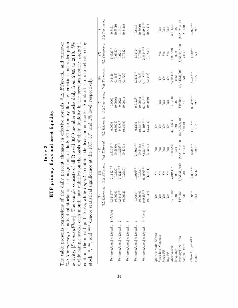
variables, on the most-liquid and least-liquid stocks. The results are reported in Table 3.

Insert Table 3 About Here

Table 3 Column 1 shows that there is a differential association of individual stocks’

trading activity with daily ETF primary flows in dollar terms. On days with larger ETF

primary flows, in either direction (i.e. positive or negative), ex ante liquid stocks’ liquidity

improved while ex ante illiquid stocks’ liquidity worsened. However, as Figure 2 panel B

showed, ETF primary flows have increased steadily throughout our sample period; hence,

we scale the daily dollar amounts so that that our main independent variable has a stationary

distribution. Table 3 Column 2 repeats the estimates, scaling the daily ETF primary flows

by the total AUM in the sample ETFs as of the previous business day. The results are the

same.

18

Table 3 Columns 3 and 4 break the sample into days when the total ETF primary flow

was positive (column 3) versus days when it was negative (column 4). In these disjoint

subsamples, we see consistent and symmetric results: the larger the magnitude of ETF

primary flow, in either direction, the larger the bifurcation of individual stocks’ liquidity.

For trading activity (share turnover) in individual stocks, the pattern is in the opposite

direction. Table 3 Columns 5 through 8 show that regardless of the unit of measurement,

and symmetrically, a larger magnitude of ETF primary flows in either direction is associated

with a relative decrease in trading activity in illiquid stocks. These results are consistent

with the main predictions of our model.

C. Replicator versus Sampler ETFs and Stock Liquidity

A key prediction that is unique to our model is that ETFs that follow a sampling strat-

egy should cause a bigger differential effect in asset markets than ETFs that follow a full-

replication strategy. From an investor’s point of view there is no difference between an ETF

that samples and an ETF that fully replicates. Because an ETF’s replication strategy is set

at inception, and because investors are indifferent – indeed ignorant – if they are trading

a replicator or sampler, confounding factors such as news arrival, algorithmic trading, or

investor behavior predict no difference in the relation for replicator versus sampler funds.

Thus, comparing the effects of primary flows through the two types of ETF is a clean test

of our model.

One concern with such a comparison is that replicator and sampler funds differ on other

dimensions. For example, funds that track an index of large liquid assets such as the S&P500

are more likely to be fully replicating, while funds that track an index containing small and

illiquid assets such as the Russell 2000 are more likely to be samplers. This fact is consistent

19

with the main hypothesis of our paper, but it potentially distorts the comparison between

replicator and sampler ETFs’ effects.

To address this concern, we construct a matched set of replicator and sampler ETFs. For

each fund-year in our data that is a sampler (i.e. replicates their target index statistically

and is not fully replicating), we attempt to match it to a replicator fund in the same year.

Matched fund-year pairs must have the same detailed four-character CRSP objective code

and assets under management (AUM) at the beginning of the year that is within 25% of

each other. When there are multiple matches we pick the closest match in terms of AUM.

For example, the ALPS Dividend Dogs ETF (ticker SDOG, AUM $1.86B, replicator), which

tracks a subset of the SP500 index consisting of the five firms in each sector with the highest

dividend yield, is matched with the WisdomTree U.S. Large-Cap Dividend Fund (ticker

DLN, AUM $1.88B, sampler) which tracks the 300 largest companies ranked by market

capitalization from the WisdomTree U.S. Dividend Index. Thus, these are two large-cap

dividend funds, which began the year with almost identical assets under management.

In all we construct 599 matched fund-year pairs, for an average of 60 matched pairs per

year. The average total AUM per year in 2018 dollars is $114B for the sampler funds and

$118B for the replicator funds, so the average sampler (replicator) fund has $1.90B ($1.97B)

in assets under management. Figure 4 compares the distributions of fund AUM, expense

ratio and turnover between the matched samples. By construction, the distributions of fund

AUM are nearly identical. The replicator funds have slightly higher expense ratios and

slightly lower turnover on average, but overall the distributions of those fund characteristics

are also very similar.

Insert Figure 4 About Here

Table 4 compares the effects of daily ETF primary flows, between the matched ETFs

20

that are replicators versus samplers.

Insert Table 4 About Here

We see that primary flows for both types of ETF affect trading activity (share turnover)

in a consistent direction (Columns 2 and 4). However, the effects of ETF primary flow on

liquidity are of opposite sign between the two types of ETF. Primary flows for replicator

ETFs (column 1) are associated with a relative improvement to liquidity for illiquid stocks,

which is also much smaller than the effects we document. By contrast, and consistent with

our main results, primary flows for sampler ETFs (column 3) are associated with a relative

fall in liquidity for illiquid stocks and vice versa. The different signs between different types

of ETF are consistent with our model’s specific predictions, and are difficult to explain via

other confounding factors because (i) the matched fund pairs follow similar indexes and have

similar assets under management, and (ii) traders and investors are indifferent whether a

given fund is a replicator or a sampler.

In summary, ETFs overweight (underweight) the index underlying assets that are ex ante

liquid (illiquid). This creates a “Matthew effect” that makes the liquid (illiquid) assets even

more liquid (illiquid). In the next section, we test some alternative explanations.

IV. Alternative explanations

One concern with our results is that market dynamics change over time, and could covary

with both ETF turnover and stock turnover and liquidity. For example, the arrival of

index-relevant information could drive increased ETF trading activity, and also cause market

makers to reduce their trading activity and widen their bid/ask spreads, particularly in less

liquid stocks. We examine these potential confounds in two ways.

21

First, it could be that when there is market-moving news (or the risk of market-moving

news arriving), market makers reduce liquidity more in stocks that were less liquid ex ante.

To examine this possibility, we first add the magnitude (absolute value) of the CRSP value-

weighted U.S. market index as an additional explanatory variable, interacted with each

stock’s lagged liquidity quintile. Table 5 columns 1 and 2 show that the relationship between

ETF primary flows and asset liquidity is effectively unchanged when we add the daily market

return as an additional explanatory factor (compare with Table 3 column 3).

Insert Table 5 About Here

Second, we drop from the sample any days in which the U.S. stock market had a return

outside the range [-0.5%, +0.5%]. This filter leaves us with a subsample of 1,291 trading

days on which the stock market hardly moved. Table 5 columns 3 and 4 show the results.

The differential relationship between ETF primary flows and stock liquidity is even stronger

than in the full sample, particularly for the least liquid set of underlying stocks, and the

relationship with stock-level trading activity is again apparent. Thus, in the absence of

market-moving news, on quiet market days, the relationship between ETF primary flows

and stock liquidity is actually stronger than on days when the market moved a lot.

The third way that we examine the influence of other market factors is to control for

time-varying factors such as high frequency trading activity and market fragmentation. We

use the SEC MIDAS data to construct measures of both high frequency trading activity

(Trade to order ratio) (Weller, 2017) and market fragmentation (HHI of trading volume

across market venues), for each stock by month individually from 2012 to 2018. The results

when we add those stock-level measures as controls are shown in Table 6.

Insert Table 6 About Here

22

We see that the differential relations of daily total ETF primary flow with stock liquidity

and turnover are still present, both across all days in the more recent sample (columns 1

and 2) and when we condition down to days on which the market did not move (columns 3

and 4). We conclude that daily stock-level changes in high frequency trading activity and

market fragmentation do not subsume our results.

V. Conclusion

An index fund or ETF’s objective is to deliver a low expected tracking error at a low expected

cost. In this paper we document the direct consequences of ETF replication strategy, most

prominently a bifurcation effect on the liquidity of the underlying index assets. Liquid stocks

become more liquid, and illiquid stocks become more illiquid, due to ETF trading activity.

We construct a stylized model to characterize the trade-off between tracking error and

trading cost. The model predicts that for stocks that are illiquid and expensive to trade,

index funds and ETF providers are better off underweighting or omitting these stocks. This

is an important point for the academic literature on the effects of the rise of index investing.

Our contribution is two-fold. First, although comovement in stock liquidity is well studied

over the past two decades, the widening liquidity gap in the U.S. stock market since 2006 has

received little attention. Our theory not only helps explain this fact, but also predicts that

as long as ETF trading activity continues to increase the liquidity gap is expected to widen

even further. Second, we point out a treatment effect that has been ignored by empirical

studies in this field – index constituents being systematically underweighted or omitted from

the ETF basket. Mistakenly classifying omitted stocks as treated stocks (as will happen

using either index weights or index assignment to proxy for fund ownership) can result in

23

biased estimates of the effects of index investing. Thus, our results should inform future

empirical research as well.

24

References

Agarwal, V., Hanouna, P., Moussawi, R., & Stahel, C. W. (2018). Do ETFs increase the

commonality in liquidity of underlying stocks? Working Paper .

Angel, J. J., Harris, L. E., & Spatt, C. S. (2015). Equity trading in the 21st century: An

update. Quarterly Journal of Finance, 5 (1), 1–39.

Basak, S., Pavlova, A., & Shapiro, A. (2007). Optimal asset allocation and risk shifting in

money management. Review of Financial Studies , 20 (5), 1583–1621.

Ben-David, I., Franzoni, F., & Moussawi, R. (2018). Do ETFs increase volatility? Journal

of Finance, 73 (6), 2471–2535.

Blocher, J., & Whaley, R. E. (2016). Two-sided markets in asset management: Exchange-

traded funds and securities lending. Working Paper .

Carpenter, J. N. (2000). Does option compensation increase managerial risk appetite?

Journal of Finance, 55 (5), 2311–2331.

Da, Z., & Shive, S. (2018). Exchange traded funds and asset return correlations. European

Financial Management , 24 (1), 136–168.

Evans, R. B., Moussawi, R., Pagano, M. S., & Sedunov, J. (2019). ETF short interest and

failures-to-deliver: Naked short-selling or operational shorting? Working Paper .

Goldstein, I., Li, Y., & Yang, L. (2013). Speculation and hedging in segmented markets.

25

Review of Financial Studies , 27 , 881-922.

Greenwood, R. (2007). Excess comovement of stock returns: Evidence from cross-sectional

variation in Nikkei 225 weights. Review of Financial Studies , 21 (3), 1153–1186.

Haslag, P. H., & Ringgenberg, M. (2016). The causal impact of market fragmentation on

liquidity. Working Paper .

Hendershott, T., Jones, C. M., & Menkveld, A. J. (2011). Does algorithmic trading improve

liquidity? Journal of Finance, 66 (1), 1–33.

Holden, C. W., & Jacobsen, S. (2014). Liquidity measurement problems in fast, competitive

markets: Expensive and cheap solutions. Journal of Finance, 69 (4), 1747–1785.

Hortacsu, A., & Syverson, C. (2004). Product Differentiation, Search Costs, and Competition

in the Mutual Fund Industry: A case study of S&P 500 index funds. Quarterly Journal

of Economics , 119 (2), 403-456.

Israeli, D., Lee, C. M., & Sridharan, S. A. (2017). Is there a dark side to exchange traded

funds? An information perspective. Review of Accounting Studies , 22 (3), 1048–1083.

Jones, C. M. (2013). What do we know about high-frequency trading? Working Paper .

Kyle, A. S. (1985). Continuous auctions and insider trading. Econometrica, 53 (6), 1315–

1335.

Lee, C. M., & Ready, M. J. (1991). Inferring trade direction from intraday data. Journal of

26

Finance, 46 (2), 733–746.

Lettau, M., & Madhavan, A. (2018). Exchange-traded funds 101 for economists. Journal of

Economic Perspectives , 32 (1), 135–54.

Malamud, S. (2016). A dynamic equilibrium model of ETFs. Working Paper .

Pan, K., & Zeng, Y. (2019). ETF arbitrage under liquidity mismatch. Working Paper .

Robertson, A. (2019). Passive in name only: Delegated management and ‘index’ investing.

Yale Journal on Regulation, Forthcoming .

Saglam, M., Tuzun, T., & Wermers, R. (2019). Do ETFs increase liquidity? Working

Paper .

Weller, B. M. (2017). Does algorithmic trading reduce information acquisition? Review of

Financial Studies , 31 (6), 2184–2226.

27

0.12

50.

250.

51

2R

atio

to A

vera

ge A

mih

ud in

200

0

2000 2005 2010 2015

High Liquidity Medium Liquidity Low Liquidity

(a) Amihud price impact

0.12

50.

250.

51

2R

atio

to A

vera

ge E

ffect

ive

Spre

ad in

200

0

2000 2005 2010 2015 2018

High Liquidity Medium Liquidity Low Liquidity

(b) Effective Spread

Figure 1. The evolution of U.S. stock liquidity

The figure plots the distribution of liquidity across U.S. common stocks over time. Stocksare sorted into terciles on the basis of their liquidity each quarter. Panel A plots quarterlyAmihuds from 1990 to 2018, while panel B plots quarterly effective spreads from 2000 to2018. The plots show the average in each tercile, by quarter, scaled by the average measurefor that tercile as of the start of the sample period. The sample includes all U.S. commonstocks with market capitalization greater than $300M in 2018 dollars.

28

0$1

T$2

T$3

T$4

TAU

M in

U.S

. Equ

ity E

TFs

2000 2005 2010 2015 2019

(a) ETF assets under management

-$20

0B-$

100B

0$1

00B

$200

B$3

00B

Prim

ary

Flow

to/fr

om U

.S. E

quity

ETF

s

2000 2005 2010 2015 2019

Creation Redemption

(b) ETF primary flows

Figure 2. ETF assets under management and primary flows

Panel A plots total assets under management and panel B plots total positive and negativeprimary flows (total dollar create and redeem activity, respectively) in U.S. equity exchangetraded funds (ETFs), quarterly from 1993 to 2018.

29

-.005

0.0

05Δ

Log(

Effe

ctiv

e Sp

read

) t

-.02 -.01 0 .01 .02ETF Primary flowt / AUM

(a) Quintile 1 (Most liquid ex ante)

-.005

0.0

05Δ

Log(

Effe

ctiv

e Sp

read

) t

-.02 -.01 0 .01 .02ETF Primary flowt / AUM

(b) Quintile 5 (Least liquid ex ante)

Figure 3. ETF primary flow and changes in asset liquidity

The figure plots daily changes in effective spreads for individual stocks, against daily totalprimary flows (total dollar creations minus redemptions scaled by AUM) for U.S. equityETFs. Panels A and B plot the relation for stocks that were in the first and fifth quintilerespectively sorted by effective spread as of the previous month (the most liquid and leastliquid stocks ex ante). The blue lines show the linear best-fit line, separately estimated forpositive and negative ETF primary flows. The dashed lines show 95% confidence intervals.

30

0.05

.1.15

.2

0 5 10 15 0 5 10 15

Replicators Samplers

Density

Log(Assets)

(a) Fund AUM

010

020

030

0

0 .005 .01 .015 0 .005 .01 .015

Replicators Samplers

Den

sity

Expense Ratio

(b) Fund expense ratio

01

23

0 .5 1 1.5 2 0 .5 1 1.5 2

Replicators Samplers

Den

sity

Turnover Ratio

(c) Fund turnover ratio

Figure 4. The figure plots histograms of log assets under management (a), expense ratios(b), and yearly turnover ratios (c), comparing the matched samples of replicator ETFs (left)and sampler ETFs (right).

31

Table 1Summary Statistics

Panel A presents summary statistics of our sample stocks, which consist of all Russell 3000members (including both the Russell 1000 large-cap index and the Russell 2000 small-capindex) monthly from 2009-2018. The sample contains 5,743 unique stocks. Panel B displayssummary statistics of ETFs in our sample, which consists of all U.S. equity ETFs in theCRSP mutual fund database from 2009-2018. The table is split on the basis of each fund’sreplication strategy.

Panel A: Index Stocks

Mean StDev P10 Median P90

Market Cap ($ Millions) 6,700 25,267 198 1,198 12,672

Amihud (%/$100 Million) 0.0137 0.0347 0.000095 0.00175 0.0356

Volatility 0.025 0.014 0.011 0.021 0.042

Panel B: Exchange Traded Funds

Observations Mean StDev P10 Median P90

Full Replication

AUM ($ Millions) 4,233 1,921 9,239 23 203 3,902

Expense Ratio (%) 4,059 0.45 0.22 0.14 0.48 0.70

Turnover 4,043 0.41 0.55 0.06 0.25 0.94

Sampling / Optimized

AUM ($ Millions) 1,279 2,802 9,894 22 282 4,725

Expense Ratio (%) 1,226 0.44 0.17 0.20 0.48 0.63

Turnover 1,220 0.28 0.28 0.05 0.20 0.61

Other

AUM ($ Millions) 425 268 538 15 60 816

Expense Ratio (%) 397 0.81 0.27 0.45 0.95 0.99

Turnover 386 1.00 2.03 0.07 0.45 2.66

32

Table 2Stock characteristics and ETF holdings

The table presents regressions of quarterly fund holdings by ETFs on the characteristics ofindex stocks. The dependent variable 1Omittedijt is a dummy variable that equals 1 if fundj omitted stock i in its holdings in quarter t, and 0 if fund j held any number of shares ofstock i in quarter t. The sample unit is stock-fund-quarter and includes all stocks that werein the Russell 1000 or 2000 index and all Russell 1000 and 2000 ETFs that reported theirholdings in quarter t, from 2009 to 2018. Standard errors are clustered by stock. *, **, and*** denote statistical significance at the 10%, 5%, and 1% level, respectively.

(1) (2) (3)

Spreadit 0.0142*** 0.0141*** 0.0148**

(0.00501) (0.00503) (0.00556)

V olatilityit 0.0163*** 0.0166*** 0.0158***

(0.00395) (0.00397) (0.00378)

Correlation w Indexit -0.00724 -0.00525 -0.00639

(0.0127) (0.0130) (0.0130)

IndexWeightit 1.683 1.663 -0.683

(2.131) (2.130) (2.531)

Fund FE Yes No No

Year-Quarter FE Yes No No

Fund x Year-Quarter FE No Yes Yes

Index Bucket FE No No Yes

Observations 1,005,002 1,005,002 1,005,002

R-squared 0.22 0.23 0.24

33

Table

3E

TF

pri

mary

flow

sand

ass

et

liquid

ity

The

table

pre

sents

regr

essi

ons

ofth

edai

lyp

erce

nt

chan

ges

ineff

ecti

vesp

read

s%

∆ESpreadit

and

turn

over

%∆Turnover

itof

indiv

idual

stock

son

the

mag

nit

ude

ofdai

lyE

TF

pri

mar

yflow

i.e.

crea

tion

and

redem

pti

onac

tivit

y,|PrimaryFlow

t|.T

he

sam

ple

consi

sts

ofal

lR

uss

ell

3000

mem

ber

stock

sdai

lyfr

om20

09to

2018

.W

ediv

ide

sam

ple

stock

sea

chm

onth

into

quin

tile

son

the

bas

isof

thei

rliquid

ity

inth

epre

vio

us

mon

th:Liquid

1co

nta

ins

the

mos

tliquid

stock

s,w

hileLiquid

5co

nta

ins

the

leas

tliquid

stock

s.Sta

ndar

der

rors

are

clust

ered

by

stock

.*,

**,

and

***

den

ote

stat

isti

cal

sign

ifica

nce

atth

e10

%,

5%,

and

1%le

vel,

resp

ecti

vely

.

(1)

(2)

(3)

(4)

(5)

(6)

(7)

(8)

%∆ESpreadit

%∆ESpreadit

%∆ESpreadit

%∆ESpreadit

%∆Turnover

it%

∆Turnover

it%

∆Turnover

it%

∆Turnover

it

|PrimaryFlow

t|×Liquid

t−1

1(M

ost)

-0.0

246*

**-2

.114

2***

-3.7

304*

**0.

0696

-0.0

069

-0.3

426

-1.4

326*

*0.

7451

(0.0

029)

(0.2

422)

(0.3

680)

(0.3

924)

(0.0

046)

(0.4

162)

(0.6

622)

(0.7

509)

|PrimaryFlow

t|×Liquid

t−1

2-0

.014

1***

-1.4

726*

**-1

.927

5***

-0.8

181*

0.00

220.

8811

*0.

6219

1.04

01

(0.0

032)

(0.2

689)

(0.4

393)

(0.4

500)

(0.0

051)

(0.4

720)

(0.7

322)

(0.8

418)

|PrimaryFlow

t|×Liquid

t−1

3-

--

--

--

-

|PrimaryFlow

t|×Liquid

t−1

40.

0065

*1.

4916

***

2.48

67**

*0.

1206

-0.0

123*

*-1

.023

2**

-1.3

472*

-0.6

536

(0.0

040)

(0.3

524)

(0.5

496)

(0.5

847)

(0.0

054)

(0.4

767)

(0.7

591)

(0.8

909)

|PrimaryFlow

t|×Liquid

t−1

5(Least

)0.

0845

***

9.90

56**

*8.

6286

***

11.1

198*

**-0

.042

1***

-3.1

018*

**-2

.862

4***

-3.6

285*

**

(0.0

117)

(1.4

671)

(1.5

107)

(3.2

305)

(0.0

069)

(0.5

148)

(0.7

853)

(0.8

717)

Qu

inti

leM

ain

Eff

ects

Yes

Yes

Yes

Yes

Sto

ck-l

evel

Con

trol

sY

esY

esY

esY

esY

esY

esY

esY

es

Sto

ckF

EY

esY

esY

esY

esY

esY

esY

esY

es

Day

FE

Yes

Yes

Yes

Yes

Yes

Yes

Yes

Yes

Ob

serv

atio

ns

7,21

9,41

87,

219,

418

4,20

7,82

13,

011,

594

7,21

9,41

87,

219,

418

4,20

7,82

13,

011,

594

R-s

qu

ared

0.01

0.01

0.01

0.01

0.02

0.02

0.02

0.02

Pri

mar

yF

low

Un

its

$Tri

llio

n($

/AU

M)/

100

($/A

UM

)/10

0($

/AU

M)/

100

$Tri

llio

n($

/AU

M)/

100

($/A

UM

)/10

0($

/AU

M)/

100

Sam

ple

Dat

esA

llA

llC

R>

0C

R<

0A

llA

llC

R>

0C

R<

0

βLiquid

5−βLiquid

10.

109*

**12

.001

***

12.3

5***

11.0

1***

-0.0

352*

**-2

.759

***

-1.4

32**

-4.3

69**

*

F-s

tat

90.1

68.6

69.8

11.8

32.8

42.8

5.1

39.8

34

Table 4ETF primary flows and asset liquidity: Replicator vs sampler ETFs

The table presents regressions of the daily percent changes in effective spreads %∆ ESpreaditand turnover %∆ Turnoverit of individual stocks on the magnitude of daily ETF primaryflow i.e. creation and redemption activity, |PrimaryF lowt|. The daily ETF primary flowsare calculated using a matched sample of pairs of replicator and sampler fund-years thathave the same Lipper objective code and similar assets under management (AUM). Wedivide sample stocks each month into quintiles on the basis of their liquidity in the previousmonth: Liquid 1 contains the most liquid stocks, while Liquid 5 contains the least liquidstocks. Standard errors are clustered by stock. *, **, and *** denote statistical significanceat the 10%, 5%, and 1% level, respectively.

(1) (2) (3) (4)

%∆ ESpreadit %∆ Turnoverit %∆ ESpreadit %∆ Turnoverit

|PrimaryF lowt| × Liquidt−1 1 (Most) 0.21*** 0.40*** -1.47*** -0.15

(0.08) (0.13) (0.33) (0.30)

|PrimaryF lowt| × Liquidt−1 2 0.34*** 0.33** -0.24 0.36

(0.09) (0.16) (0.38) (0.35)

|PrimaryF lowt| × Liquidt−1 3 - - - -

|PrimaryF lowt| × Liquidt−1 4 -0.41*** -0.39** 0.31 -1.53***

(0.13) (0.19) (0.44) (0.56)

|PrimaryF lowt| × Liquidt−1 5 (Least) -0.63** -0.55*** 3.15*** -2.96***

(0.32) (0.17) (0.90) (0.42)

ETF Type Replicators Replicators Samplers Samplers

Quintile Main Effects Yes Yes Yes Yes

Stock-level Controls Yes Yes Yes Yes

Stock FE Yes Yes Yes Yes

Date FE Yes Yes Yes Yes

Observations 7,219,418 7,219,418 7,219,418 7,219,418

R-squared 0.01 0.02 0.01 0.02

PrimaryFlow Units ($/AUM)/100 ($/AUM)/100 ($/AUM)/100 ($/AUM)/100

βLiquid 5 − βLiquid 1 -0.85** -0.95*** 4.63*** -2.81***

F-stat 7.2 43.9 28.4 57.7

35

Table 5ETF primary flows and asset liquidity: Controlling for market-wide news

The table presents regressions of the daily percent changes in effective spreads %∆ ESpreaditand turnover %∆ Turnoverit of individual stocks on the magnitude of daily ETF primaryflow i.e. creation and redemption activity, |PrimaryF lowt|. The “No News” sample incolumns 3 and 4 consists only of days on which the market return was smaller than +/- 50basis points. We divide sample stocks each month into quintiles on the basis of their liquidityin the previous month: Liquid 1 contains the most liquid stocks, while Liquid 5 contains theleast liquid stocks. Standard errors are clustered by stock. *, **, and *** denote statisticalsignificance at the 10%, 5%, and 1% level, respectively.

(1) (2) (3) (4)

%∆ ESpreadit %∆ Turnoverit %∆ ESpreadit %∆ Turnoverit

|PrimaryF lowt| × Liquidt−1 1 (Most) 0.2148*** 0.3993*** -1.4735*** -0.1530

(0.0808) (0.1340) (0.3341) (0.3016)

|PrimaryF lowt| × Liquidt−1 2 -1.52*** -0.65 -3.61*** 0.38

(0.31) (0.54) (0.70) (1.10)

|PrimaryF lowt| × Liquidt−1 3 - - - -

|PrimaryF lowt| × Liquidt−1 4 0.42 -0.82 1.98** -0.97

(0.41) (0.54) (0.90) (1.12)

|PrimaryF lowt| × Liquidt−1 5 (Least) 9.06*** -1.51*** 17.03*** -3.11***

(2.15) (0.57) (4.07) (1.14)

|Benchmark Retit| × Liquidt−1 1 -0.00* 0.01*** -0.01* 0.02**

(0.00) (0.00) (0.01) (0.01)

|Benchmark Retit| × Liquidt−1 2 0.00 0.01*** -0.00 0.03***

(0.00) (0.00) (0.00) (0.01)

|Benchmark Retit| × Liquidt−1 3 - - - -

|Benchmark Retit| × Liquidt−1 4 0.01*** -0.00 0.02*** 0.02***

(0.00) (0.00) (0.01) (0.01)

|Benchmark Retit| × Liquidt−1 5 0.01 -0.01*** 0.02 0.02***

(0.01) (0.00) (0.01) (0.01)

Sample Dates All All No News No News

Quintile Main Effects Yes Yes Yes Yes

Stock-level Controls Yes Yes Yes Yes

Stock FE Yes Yes Yes Yes

Date FE Yes Yes Yes Yes

Observations 7,219,418 7,219,418 3,834,554 3,834,554

R-squared 0.01 0.02 0.01 0.02

PrimaryFlow Units ($/AUM)/100 ($/AUM)/100 ($/AUM)/100 ($/AUM)/100

βLiquid 5 − βLiquid 1 10.95*** -0.196 22.02*** -2.033**

F-stat 26.2 0.2 29.6 5.3

36

Table 6ETF primary flows and asset liquidity: Controlling for market fragmentation

and HFT activity

The table presents regressions of the daily percent changes in effective spreads %∆ ESpreaditand turnover %∆ Turnoverit of individual stocks on the magnitude of daily ETF primaryflow i.e. creation and redemption activity, |PrimaryF lowt|. The Herfindahl of tradingvolume across venuesHHIit measures market fragmentation. The trade-to-order ratio TORit

measures high frequency trading activity. The results are similar using other measures suchas Odd-lot ratio, average trade size, and cancel-to-trade ratio. We divide sample stocks eachmonth into quintiles on the basis of their liquidity in the previous month: Liquid 1 containsthe most liquid stocks, while Liquid 5 contains the least liquid stocks. Standard errors areclustered by stock. *, **, and *** denote statistical significance at the 10%, 5%, and 1%level, respectively.

(1) (2) (3) (4)

%∆ ESpreadit %∆ Turnoverit %∆ ESpreadit %∆ Turnoverit

|PrimaryF lowt| × Liquidt−1 1 (Most) -3.90*** 1.68* -7.97*** 2.03

(0.68) (0.93) (1.04) (1.53)

|PrimaryF lowt| × Liquidt−1 2 -1.58** 2.17** -4.42*** 3.20**

(0.77) (0.97) (1.35) (1.57)

|PrimaryF lowt| × Liquidt−1 3 - - - -

|PrimaryF lowt| × Liquidt−1 4 -1.86** -3.50*** 0.17 -2.71*

(0.92) (1.01) (1.67) (1.53)

|PrimaryF lowt| × Liquidt−1 5 (Least) 6.57*** -10.43*** 11.71*** -11.20***

(2.17) (1.14) (3.87) (1.68)

HHIit 0.11*** 0.08*** 0.13*** 0.09***

(0.03) (0.01) (0.04) (0.01)

TORit -1.29*** 11.56*** -1.20*** 11.83***

(0.05) (0.20) (0.06) (0.27)

Sample Dates All All No News No News

Control for Market Returns Yes Yes Yes Yes

Quintile Main Effects Yes Yes Yes Yes

Controls Yes Yes Yes Yes

Stock FE Yes Yes Yes Yes

Date FE Yes Yes Yes Yes

Observations 4,527,432 4,527,432 2,646,165 2,646,165

R-squared 0.02 0.04 0.02 0.04

PrimaryFlow Units ($/AUM)/100 ($/AUM)/100 ($/AUM)/100 ($/AUM)/100

βLiquid 5 − βLiquid 1 10.47*** -12.11*** 19.68*** -13.24***

F-stat 24.9 127.5 27.4 70.1

37

Appendix

A. Variable Definitions

Table A1: Variable Definitions

Variable Names Description

%∆ESpread The percentage change in effective spread of stock i on day tis calculated as following:

%∆ESpreadi,t = log(ESpreadi,t)− log(ESpreadi,t−1)

%∆Turnover The percentage change in turnover of stock i on day t is cal-culated as following:

%∆Turnoveri,t = log(Turnoveri,t)− log(Turnoveri,t−1)

1Omitted Dummy variable that equals 1 if ETF j omitted stock i inquarter t.

Amihud Absolute value of monthly return of stock i divided bymonthly dollar trading volume in month t. Monthly dollartrading volume is calculated as monthly share trading volumetimes end of month closing price.

AUM (ETF) Price of ETF i times shares outstanding of ETF i on day t.

Benchmark Retit Russell 1000 or Russell 2000 Index return, depending on whichone stock i belongs to, on day t.

Correlation with Index The correlation between daily returns of stock i and the dailyreturns of the index that includes stock i in quarter t

.

Continued on next page

38

Table A1 – continued from previous page

Variable Definitions Description

Effective Spread Let i denote stock, t denote day, and s denote intraday time.The dollar-weighted percentage effective spread of stock i onday t is calculated as following:∑

s

| log(priceits)− log(midpointits)| · priceits · sizeits∑s priceits · sizeits

Buy-sell indicator are created using method in Lee and Ready(1991) and quotes prior to 2015 are interpolated using methodin Holden and Jacobsen (2014).

Expense Ratio Expense ratio of ETF i in year t from CRSP Mutual FundDatabase.

HHI Let i denote stock, j denote exchange, and t denote month.Herfindahl-Hirschman Index is calculated monthly as follow-ing:

HHIit =∑j

(Trading Volumeijt∑j Trading Volumeijt

)2

Index Weight Stock i ’s weight in index j at month t, from Russell proprietarydata.

Market Cap Closing price of stock i times shares outstanding of stock i onday t.

Primary Flow, dollar unit The change of the shares outstanding of ETF i from day t-1to day t times closing price of ETF i on day t.

Primary Flow, percent unit The dollar unit primary flow of ETF i on day t divided bythe AUM of ETF i on day t, calculated daily.

Continued on next page

39

Table A1 – continued from previous page

Variable Definitions Description

TOR Trade to order ratio, calculated as the trading volume of stocki on day t divided by the order volume of stock i on day t.

Turnover Trading volume of ETF i divided by shares outstanding ofETF i on day t.

Volatility Standard deviation of daily return of stock i in month t.

B. Further discussion of the model

B.1. Open-ended index funds

As noted before, our model also applies to traditional open-ended index funds that rebalance

their portfolios after inflows and outflows. The index fund manager chooses their replication

strategy to attract investors, who again have the same utility function over expected tracking

error and expected trading costs (which investors now bear directly via the management fee,

instead of indirectly via the bid/ask spread):

U = C(w) + λ(w − v)′Σ(w − v)

The rest of the solution and all comparative statics are the same.

B.2. Trading in index futures

Recall that

40

w∗i =1

1 + ci/λσ2i

vi +1

1 + ci/λσ2i

∑j 6=i

(vj − wj)βj,i

Consider an index for which there is a liquid futures contract. The futures contract has

vi = 0, so the first term is zero. That is, the futures contract is not an index constituent, and

for such assets we would think w∗i should also be zero. But the futures contract is perfectly

correlated with the weighted return of the index constituents, and has very low trading costs

ci. In this case, the optimal weights wj on all the index constituents themselves are close to

zero and the optimal weight on the futures contract is close to one.

B.3. Redundant assets

Recall that

w∗i =1

1 + ci/λσ2i

vi +1

1 + ci/λσ2i

∑j 6=i

(vj − wj)βj,i

Consider two perfectly substitutable assets (ρ1,2 = 1) with different relative trading costs

(c1/σ21 6= c2/σ

22). Assume for simplicity that ρ1,j, ρ2,j = 0,∀j 6= 1, 2.8 We have a system of

equations with two equations and two unknowns:

8More general case with arbitrary ρ gives the same qualitative result.

41

w∗1 = κ1v1 + κ1v2σ2σ1− κ1w2

σ2σ1

w∗2 = κ2v2 + κ2v1σ1σ2− κ2w1

σ1σ2

where

κi =1

1 + ci/λσ2i

Solve for:

w∗1 =κ1(1− κ2)1− κ1κ2

(v1 +

σ2σ1v2

)

Note that, if security one is almost costless to trade, then κ1 → 1, and w∗1 = v1+v2(σ2/σ1).

In other words, security one completely takes security two’s place in the basket. Alternatively,

if security one is infinitely expensive to trade, then κ1 → 0 and its optimal weight is zero.

Between the two corner solutions, the optimal weights tilt in favor of holding the asset that

is relatively cheaper to trade. The cheaper asset does not completely take over because of

the quadratic trading cost.

B.4. Short selling revenues

On top of the utility function used in our paper and discussed above in appendix, fund

managers may have additional incentives to hold certain assets if they collect the lending

42

fees from offering their shares to short sellers (Blocher & Whaley, 2016). Short borrow fees

will shift the optimal holdings, but has no impact on our other directional predictions. To

see this, consider the modified utility function:

U = C(w)− S′w + λ(w − v)′Σ(w − v)

where S is the expected short borrow fee per asset, which offsets the expected trading

costs. Solving for asset i, we have:

w∗i =1

1 + ci/λσ2i

vi +1

1 + ci/λσ2i

∑j 6=i

(vj − wj)βj,i +1

ci + λσ2i

si

Notice that the optimal weights are higher than before, but the comparative statics with

respect to ci, ρi,j and σ2i are unchanged.

43