Region 2

UNIVERSITY TRANSPORTATION RESEARCH CENTER

The retrofit puzzle: optimal fleet owner behavior in the context of diesel retrofit incentive programs

Prepared by

H. Oliver Gao, Ph.D. Timon H. Stasko

School of Civil and Environmental Engineering

Cornell University Ithaca, NY 14853 USA

December 31, 2007

Disclaimer The contents of this report reflect the views of the authors, who are responsible for the facts and the accuracy of the information presented herein. The contents do not necessarily reflect the official views or policies of the UTRC or the Federal Highway Administration. This report does not constitute a standard, specification or regulation. This document is disseminated under the sponsorship of the Department of Transportation, University Transportation Centers Program, in the interest of information exchange. The U.S. Government assumes no liability for the contents or use thereof.

1 . Re p o r t N o . 2. Government Accession No.

TECHNICAL REPORT STANDARD TITLE PAGE

3. Rec ip ient ’s Cata log No.

5 . Repor t Date

8. Performing Organization Report No.

6 . Performing Organizat ion Code

4. Ti t le and Subt i t le

7. Author(s)

9. Performing Organization Name and Address 10. Work Unit No.

11. Contract or Grant No.

13. Type of Report and Period Covered

14. Sponsoring Agency Code

12. Sponsoring Agency Name and Address

15. Supplementary Notes

1 6 . Abstract

1 7 . Key Words

1 9 . Security Classif (of this report)

F o r m D O T F 17 0 0 . 7 ( 8 - 6 9 )

2 0 . Security Classif. (of this page)

1 8 . Distribution Statement

21. No of Pages 2 2 . Price

December 31, 2007

49777-1418 (subcontract No.)

Final Report – January – December 2007

School of Civi l and Environmental Engineer ing Cornel l Univers i ty I thaca, NY 14853 USA

University Transportation Research Center – Region 2 138 t h Street and Convent Avenue, NYC, NY 10031

Potential government regulations and financial incentives for encouraging pollution reduction retrofits on diesel vehicles are discussed. An integer program is developed to model profit-maximizing fleet owner behavior in the context of potential government programs. The model is intended as a tool both for fleet owners and for government administrators. It allows for mandated retrofits, mandated percent reductions of specified emissions, fixed grants for performing retrofits, and grants per gram of pollution prevented. It treats the fleet size and miles remaining for each vehicle as fixed and known at the time retrofits are made. Retrofits are all assumed to take place in the present, but benefits and costs are distributed over time. A case study is used to demonstrate how a sample fleet owner would respond to various incentives. Potential directions for future research are discussed.

Diesel re trof i ts ; Prof i t maximizat ion: Emission reduct ions; In teger programming

Unclass if ied Unclass if ied

46

H. Oliver Gao, Ph.D. , Timon H. Stasko

The re trof i t puzzle: opt imal f leet owner behavior in the context of d iesel re trof i t

The retrofit puzzle: optimal fleet owner behavior in the context of diesel retrofit incentive programs

H. Oliver Gao1,*, Timon Stasko2

1 H. Oliver Gao, Ph.D.School of Civil and Environmental EngineeringCornell UniversityIthaca, NY 14853 USA(607) 254-8334(607) 255-9004 FAXhg55@cornell.edu* Corresponding Author

2 Timon H. Stasko, GRASchool of Civil and Environmental EngineeringCornell UniversityIthaca, NY 14853 USAths9@cornell.edu

* 2. Manuscript

Abstract

Potential government regulations and financial incentives for encouraging

pollution reduction retrofits on diesel vehicles are discussed. An integer program is

developed to model profit-maximizing fleet owner behavior in the context of potential

government programs. The model is intended as a tool both for fleet owners and for

government administrators. It allows for mandated retrofits, mandated percent reductions

of specified emissions, fixed grants for performing retrofits, and grants per gram of

pollution prevented. It treats the fleet size and miles remaining for each vehicle as fixed

and known at the time retrofits are made. Retrofits are all assumed to take place in the

present, but benefits and costs are distributed over time. A case study is used to

demonstrate how a sample fleet owner would respond to various incentives. Potential

directions for future research are discussed.

Keywords: Diesel retrofits; Profit maximization: Emission reductions; Integer

programming

1

1. Introduction

Air pollution is an issue of growing importance to the public health, ecosystem,

and social welfare (National Research Council, 2004). As our understanding of the

science of emissions improves, the severity of their impact on public health is becoming

increasingly clear. Vehicles in particular emit large amounts of nitrogen oxides (NOx),

particulate matter (PM), hydrocarbons (HC), and other damaging pollutants. The U.S.

Environmental Protection Agency (EPA) attributes thousands of instances of premature

mortality, hundreds of thousands of asthma attacks, and millions of lost work days to

particulate matter and nitrogen oxides emissions (U.S. Environmental Protection Agency,

2007a). Vehicle emissions are also a major culprit in global warming. According to the

EPA, the transportation sector was the second largest contributor to U.S. greenhouse gas

emissions in 2005, slightly behind electricity generation (U.S. Environmental Protection

Agency, 2007b).

With the passage of the Clean Air Act (CAA) in the 1970’s and subsequent

amendments in the 1990’s, the U.S. government began addressing the problem. National

Ambient Air Quality Standards (NAAQS) were declared, and a system was put in place

to enforce them at both regional and local scales. The system allows for context-

appropriate solutions through state implementation plan (SIP) development,

transportation conformity rules, and other National Environmental Policy Act (NEPA)

procedures. Despite laudable efforts, NAAQS have proven extremely difficult to meet in

some cases, with some areas of the country seemingly stuck in non-attainment status.

EPA maps reveal that major urban areas across the country fail to meet the 8-hour ozone

2

requirements, as do selected non-urban areas and several entire states (U.S.

Environmental Protection Agency, 2007c).

One of the challenges facing administrators is that no matter how strict emission

standards become for new vehicles, it will be many years before older vehicles that

operate outside those standards are off the road. This delay is particularly pronounced

with diesel vehicles. Heavy-duty trucks and busses use diesel engines largely because of

their reliability and relatively low operating cost. This reliability means that their average

lifespans are substantially greater than those of gasoline powered cars. Diesel vehicles

already on the road today could very well be in use for another 25 years and drive close

to a million miles before being retired (U.S. Environmental Protection Agency, 2007d).

Furthermore, the size of the current fleet is substantial. There are over 11 million diesel

engines operating in the existing fleet (U.S. Environmental Protection Agency, 2007a).

These vehicles fill vital roles in our economy including freight transportation,

construction, port operations, and public transportation. Over the past decade, the

maximum allowable particulate matter and nitrogen oxides emissions for new diesel

trucks and busses have been reduced by an order of magnitude (U.S. Environmental

Protection Agency, 2003), but much of this existing fleet is not bound by these tighter

restrictions.

Unfortunately, applying the same standards to the older vehicles is not a viable

option. The cost would simply be prohibitive. Nonetheless, older vehicles cannot be

ignored when addressing our emissions problem. The health effects of diesel exhaust are

real and immediate. Lower pollution levels in twenty years are not an adequate solution

for people who are developing health problems today. According to a report by The

3

Clean Air Task Force, fine particulate matter from diesels shortens the lives of nearly

21,000 people every year (Clean Air Task Force, 2005). The same report states that

“nationally, diesel exhaust poses a cancer risk that is 7.5 times higher than the combined

total cancer risk from all other air toxics.” (Clean Air Task Force, 2005)

Fortunately, diesel retrofit options are available. Fuel delivery and air intake

systems can be optimized (U.S. Environmental Protection Agency, 2007d). Particle traps

and catalytic converters can treat exhaust before it exits the vehicle, transforming harmful

pollutants into more benign compounds (U.S. Environmental Protection Agency, 2007d).

Unfortunately, all of these upgrades come at a cost. Implementing every possible upgrade

on every existing vehicle is simply not feasible. The question becomes: which subset of

potential retrofits is optimal?

Society’s objective is to minimize the total cost – both the direct expense of

upgrades, and the externality imposed on society when upgrades are not made.

Responsible government policy must take both types of costs into account. Policy makers

must consider that upgrades will not have the same effect on all vehicles. In particular,

older vehicles may experience a greater emission reduction from an upgrade, but older

vehicles are also likely to be retired sooner. Furthermore, upgrades might influence each

others’ effectiveness. Fleet owners are unlikely to be able to take large numbers of trucks

off the road for upgrades at once, so practical scheduling is essential.

Each upgrading strategy has its own strengths, weaknesses and

variability/uncertainty in emission reduction efficiency1. The emissions reductions due to

1 Engine replacements and recalibration can be effective and may result in enhanced fuel economy and lower maintenance costs, but can be expensive. Switching to cleaner fuels might be easy, as in the case of switching to lower sulfur fuel or biodiesel blends, but has nominal air quality benefit on its own. Switching to alternative fuels, like natural gas, can be very effective, but one has to establish a new fueling and

4

retrofits are subject to many uncertain external factors, including environmental factors

(e.g., temperature, humidity), fleet characteristics (e.g., age distribution of fleet,

distribution of VMT by vehicle class, number and types of vehicles), activity measures

(e.g., speed distributions, distribution of VMT by roadway type), and fuel characteristics

(e.g., sulfur content, Reid vapor pressure (RVP)) (U.S. Environmental Protection

Agency, 2006e). Retrofit devices need to be used in the right application. Even with good

certified retrofitting technologies, unwise decisions in operations and deployment of a

retrofit program could significantly limit the benefit.

In addition to determining which retrofit implementations are wise, the

government must decide how to encourage fleet owners to conduct them. Without

regulation or incentives, fleet owners can’t necessarily be counted on to make upgrades.

The primary justification for retrofits is an externality which substantially affects large

numbers of people, but not a firm’s profit maximization. How can the government

encourage fleet owners to conduct justified retrofits, while stimulating development of

new upgrades and not imposing undue costs on fleet owners?

In order to develop such policies, the government will have to predict fleet owner

behavior. This paper outlines an integer programming model to better understand profit

maximizing retrofit selection, in the context of possible government programs. It allows

for mandated retrofits, mandated percent reductions of specified emissions, fixed grants

for performing retrofits, and grants per gram of pollution prevented. It treats the miles

remaining for each vehicle as fixed and known. The fleet size is also regarded as fixed

maintenance infrastructure in addition to engine and fuel system modifications. Aftertreatment devices need to be used in the right application and are generally effective only for two or three of the four targeted categories of pollutants (PM, NOx, hydrocarbons, and CO). Anti-idling strategies are a winner across almost all applications and save fuel and money. However, these programs are difficult to monitor, quantify and enforce.

5

and known. Retrofits are all assumed to take place in the present, but benefits and costs

are distributed over time. When run, the program reveals which retrofits will be

conducted, what costs are borne by whom, and what emission reductions are experienced.

Before describing the model formulation, the paper provides literature review

covering past work on diesel retrofits and similar integer programs. Next, potential

government policies are outlined and a subgroup is selected for use in the model. Once

the selections have been described, the model is formulated. The formulation is followed

by a case study. Finally, applications and avenues for future research are discussed.

2. Literature Review

There is little previous work on optimization models for fleet owners and diesel

retrofit program managers to assist them in making informed decisions on their diesel

fleet and retrofit programs respectively. Applicable research generally falls into one of

two categories: a) research done by or for government agencies on the viability,

efficiency, effectiveness, and cost of retrofits or b) research done on integer programs for

related problems.

In order to reduce diesel emissions, the EPA collaborates with the state and local

governments as part of the National Clean Diesel Campaign (NCDC). The program

includes technical and financial assistance to fleet owners looking to lessen emissions

from their fleets, as well as regulation (U.S. Environmental Protection Agency, 2007a).

The EPA’s National Mobile Inventory Model (NMIM) can be used to quantify emission

reductions from retrofits (U.S. Environmental Protection Agency, 2006a). NMIM

includes two EPA emission estimation programs: MOBILE 6.2 for on-road emissions and

NONROAD for off-road emissions (U.S. Environmental Protection Agency, 2006b). The

6

EPA publishes documentation on the development of these models, as well as

information on verified retrofits.

The California Air Resources Board set up the Carl Moyer Memorial Air Quality

Standards Attainment Program to provide incentives for cleaner than required vehicles

(California Air Resources Board, 2007a). Like the EPA, they publish information on

retrofits that they verify (California Air Resources Board, 2007b). They also publish

descriptions of the criteria they use for selecting retrofit projects to support (California

Air Resources Board, 2006).

The EPA published a report analyzing the cost effectiveness of retrofits for

reducing particulate matter emissions from selected heavy-duty vehicles (U.S.

Environmental Protection Agency, 2006c). In particular, the report looked at two

principle types of retrofit technologies: diesel oxidation catalysts (DOCs) and catalyzed

diesel particulate filters (CDPFs) (U.S. Environmental Protection Agency, 2006c). They

calculated the approximate cost per ton of reducing PM emissions on selected vehicle

types using these retrofits. After comparing their results with the costs of other programs,

they found retrofits could be a cost effective way to reduce air pollution (U.S.

Environmental Protection Agency, 2006c). In addition, Schipper (2005) analyzed the

impact of a pilot project of retrofits on buses in Mexico City. The primary goal of the

study was to analyze the impact of Mexico City’s high altitude on the retrofits’

effectiveness. The findings from both studies are important, and the analyses used to

produce the results are highly relevant, but they provide no means of predicting fleet

owner behavior in the context of multiple government programs. They also only provide

cost effectiveness estimates of a small subset of potential retrofit options.

7

Independently, integer programs have been developed for problems with similar

characteristics to the fleet owner’s retrofit selection. Marsten and Muller (1980)

published a profit maximizing mixed integer program for assigning planes to air cargo

movements. More recently, Janic published another integer program for a profit

maximizing airline operator selecting how many planes to fly on each route (Janic, M.,

2003). Similar to diesel fleet owners, the airline operators in Janic’s model are bound by

constraints imposed by the government to control externalities. Janic’s model does not

include government subsidies or taxes which would directly impact the airline’s profit.

Charnes et al. (1976) described a goal interval programming formulation for a

marine environmental protection program. It was designed to minimize weighted

deviations from a set of government goals. It did not, however, incorporate a model of

individuals and firms responding to government actions. Marino and Sicilian studied the

profit maximizing monopolist’s and utilility maximizing consumer’s reactions to

government regulation of utilities. In particular, the paper examined the incentive for

conservation investment given a government imposed constraint on the rate of return on

capital (Marino and Sicilian, 1988). While a related problem, the regulatory tools used for

utilities are distinctly different from those considered for fleet owners in this paper.

3. Potential Government Approaches

A multitude of potential government policies exist. In general, such polices either

require retrofits, or encourage them with incentives. More specifically, many potential

programs fit into the following categories:

1. Mandates

8

a. Mandate some percentage reduction of selected pollutants for fleets

meeting some criteria (e.g. size above 100 vehicles);

b. Mandate vehicles in a given vehicle class are upgraded with a given

technology, within fleets meeting some criteria;

c. Set maximum average grams of pollution per mile for a given

pollutant for fleets meeting some criteria.

2. Grants

a. Give money for every vehicle of a certain class receiving a specific

upgrade;

b. Give money for every gram of a specific pollutant saved by

conducting a retrofit.

3. Loans

a. Give low interest loans for certain upgrades on certain vehicle classes.

4. Taxing pollution

a. Charge fleet owners for each gram of a given pollutant their fleet

emits;

b. Charge fleet owners for each gram of a given pollutant their fleet emits

beyond a certain threshold (e.g. current emissions)2;

c. Charge fleet owners for each gram of a given pollutant their fleet

emits, and allow them to trade pollution credits;

2 Such tax programs are particularly attractive because they lower the costs imposed on fleet owners, while maintaining the incentive to reduce emissions at the margins (Vollebergh, 1997). Similar grandfathering programs were analyzed in the context of carbon emissions by Vollebergh et al. (1997) and in a general optimal tax reform context by Zodrow (1992).

9

d. Charge fleet owners for each gram of a given pollutant their fleet emits

beyond a certain threshold (e.g. current emissions), and allow them to

trade pollution credits3.

Government approaches 1a, 1b, 2a, and 2b were selected to be explicitly included

in the model of this study.

First, the government may mandate some percentage reduction of selected

pollutants for fleets meeting some criteria (e.g. size above 100 vehicles). Fleet owners

take the appropriate percentage reduction requirements for each pollutant for their fleet,

and plug them into their maximization program as constants. It is completely possible

that for some fleets and pollutants the reduction requirement will be zero.

Second, the government may mandate specific vehicle types receive specific

upgrades. This was included despite the fact that there is no choice involved on the part

of the fleet owner. The model is in no way required to predict these retrofits will take

place, but the fact that they are taking place can impact decisions made regarding other

retrofits (by changing their effectiveness, for example). They were included solely for

this reason.

Third, the government can issue grants for vehicles of a given type receiving a

specific upgrade. This has potential as a practical incentive program, which would be

feasible to execute.

Fourth, the government can issue grants per gram of specific pollutants reduced.

These grants would be challenging to administer, but they have the potential to be highly

3 A similar grandfathering program was analyzed in the context of carbon emissions by Vollebergh et al. (1997).

10

effective. The differences between these grants and the previous type are discussed in

Appendix A.

Caps on the fleet’s pollution per mile were not included as a mandate because this

would require modeling the fleet as a whole (including newly purchased vehicles not

intended to directly replace older vehicles).

While loans were not explicitly included in the model, they can be effectively

represented as a series of grants. Money paid by the government to the fleet owner would

be a positive grant, while a payment by the fleet owner back to the government would be

a negative grant.

Taxes were also not included explicitly, but from a fleet owner behavior

perspective some taxes are very similar to grants. If fleet owners were taxed per gram of

a given pollutant, it would have the same effect on their behavior as being taxed a flat fee

equal to the tax they would pay on pollution if they performed no retrofits, and then

awarded grants per gram of pollution reduced by retrofits. The marginal benefits of

retrofits would be the same. In other words, switching from grants to taxes requires we

add a constant to the objective function, which would not impact the solution of the

integer program4. On the whole, taxes would make the fleet owner less well off while

grants would make the fleet owner better off, but this is a concern when dealing with

social welfare, not when modeling fleet owner behavior. For a more detailed explanation,

see Appendix B.

Tax programs that include emissions markets cannot be accurately modeled by

the grant programs in this model. Such markets would require modeling several fleet

4 So long as the constant is non-zero the optimal objective value would change. The optimal values of the decision variables, on the other hand, would never change (Gürdal et al., 1999).

11

owners, and possibly their interactions among themselves and with the environmental

management agencies. Such a task is beyond the scope of this paper, but this paper does

provide a stepping stone for moving in such a direction.

4. Model Formulation

The set I is defined as the set of all vehicle types in the fleet, indexed by i.

Vehicles should be broken down by make, model, year, engine, expected future use, and

any past retrofits or variation that could influence the effectiveness or compatibility of

future retrofits. Let ni be the number of vehicles of type i currently in the fleet.

The set J is defined as the set of all possible retrofits, indexed by j. Each retrofit

includes a set of compatible pollutant control technologies. If the retrofit is selected, all

its technologies are applied. Cleaner fuels are considered a possible pollutant control

technology, as is replacing an older engine with a newer and cleaner engine. This permits

the model to optimize the balance between retrofitting and replacing engines. (Issues

regarding the miles remaining for a replaced engine or vehicle are discussed in Appendix

C). A fleet owner may wish to combine two or more retrofit technologies if the

combination reduces more pollutants than using either retrofit technology alone. This

combination can be considered a separate possible retrofit (in addition to each technology

alone). By treating combinations of diesel cleaning technologies in this fashion, retrofits

can influence each others’ effectiveness in a nonlinear fashion, while maintaining a linear

objective function and constraints (apart from integrality). Finally, for this formulation,

the set J includes a default case “retrofit” with no retrofitting.

The set K is the set of all relevant pollutants (e.g., NOx, PM, etc.), indexed by k.

12

The set T is the set of all time periods in which retrofit costs could be incurred or

revenues received, indexed by t with t=1 designating initial time period (when retrofit

decisions are made and retrofits are conducted). All periods are assumed to be evenly

spaced, and all costs are assumed to take place at the start of the period. Model users

(e.g., fleet managers, government agencies managing diesel retrofit) can choose the

length of periods, balancing the desire for a more accurate model (with shorter periods)

and a simpler one (with longer periods).

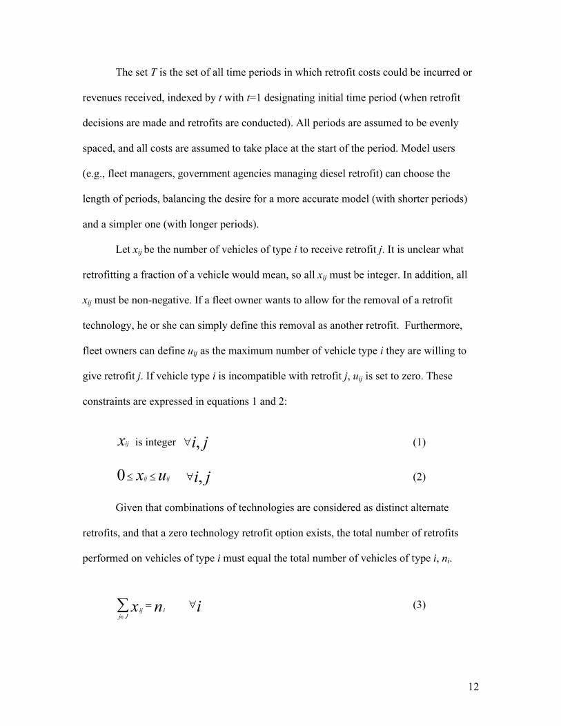
Let xij be the number of vehicles of type i to receive retrofit j. It is unclear what

retrofitting a fraction of a vehicle would mean, so all xij must be integer. In addition, all

xij must be non-negative. If a fleet owner wants to allow for the removal of a retrofit

technology, he or she can simply define this removal as another retrofit. Furthermore,

fleet owners can define uij as the maximum number of vehicle type i they are willing to

give retrofit j. If vehicle type i is incompatible with retrofit j, uij is set to zero. These

constraints are expressed in equations 1 and 2:

is integer ,ijx i j (1)

0 ,ij ijx u i j (2)

Given that combinations of technologies are considered as distinct alternate

retrofits, and that a zero technology retrofit option exists, the total number of retrofits

performed on vehicles of type i must equal the total number of vehicles of type i, ni.

ij i

j Jx n i

(3)

13

The government might require, or the fleet owner might insist, that certain

technologies are applied to some vehicle types. One might argue that because applying

such technologies is no longer a choice, they could be removed from the model without

any impact. While it is true that the model is not required to predict that the fleet owner

will conduct the required upgrades, they should still be included because of the effects

they could have on other technologies’ effectiveness.

In order to meet the emission reduction goals, the fleet owner must select retrofits

from a subset of J that includes all retrofits which include the required technologies, and

no retrofits that do not. If there are no required technologies for vehicle type i, this subset

contains all retrofits in J. Also, any retrofits which contain technologies incompatible

with vehicle type i can be removed from the subset. The resulting subset for a given

vehicle type i is called Jri. The removal of retrofit packages containing technologies

incompatible with the vehicle type is optional, however, because the incompatibility can

be sufficiently expressed by the upper bounds in expression 2. A method for representing

incompatibilities implicitly is discussed in Appendix D. Whether incompatible retrofits

are removed from Jri or not, the requirement can then be expressed as follows:

i

ij ij Jr

x n i

(4)

The time a vehicle of type i must be taken out of service to receive retrofit j is wij.

A fleet owner may have demands that must be met, and consequently can define ai as the

maximum acceptable time out of service for all vehicles of type i.

with a time-out-of-service requirementij ij ij J

x w a i

(5)

14

The opportunity cost for every unit of time a vehicle of type i is out of service is

pi. The total opportunity cost of all retrofits installed can be expressed:

ij ij ii I j J

x w p

(6)

Apart from opportunity cost, the cost of installing retrofit j on vehicle type i

incurred in period t is cijt. The parameter cijt includes the estimate of the equipment cost

for applying retrofit j to vehicle type i, cequipment_ijt, the owner’s initial installation cost,

cinstallation_ijt, and change in maintenance cost, cmaintenance_ijt. An additional cost cother_ijt is

included to capture other costs not mentioned. Some of these costs (such as installation)

may be non-zero at the initial time period, while others (such as change in maintenance

cost) may only be non-zero at later periods. All costs are expressed in dollars at the point

in time when the cost would be incurred. The total cost (less opportunity cost) of

installing retrofit j on vehicle type i, incurred in period t, is cijt:

_ _ int _ _ijt equipment ijt installation ijt ma enance ijt other ijtc c c c c , ,i j t (7)

Future costs are brought back to period 1 using an interest rate deemed

appropriate by the fleet owner. Let βt be the appropriate interest rate for bringing values

from period t back to period 1. We know that β1 will be 0, but the other values depend on

the time value of money to the fleet owner. The total cost (less opportunity cost), for all

time periods, of installing retrofit j on xij vehicles of type i can be expressed:

1

1 ij ijtt T t

x c ,i j (8)

15

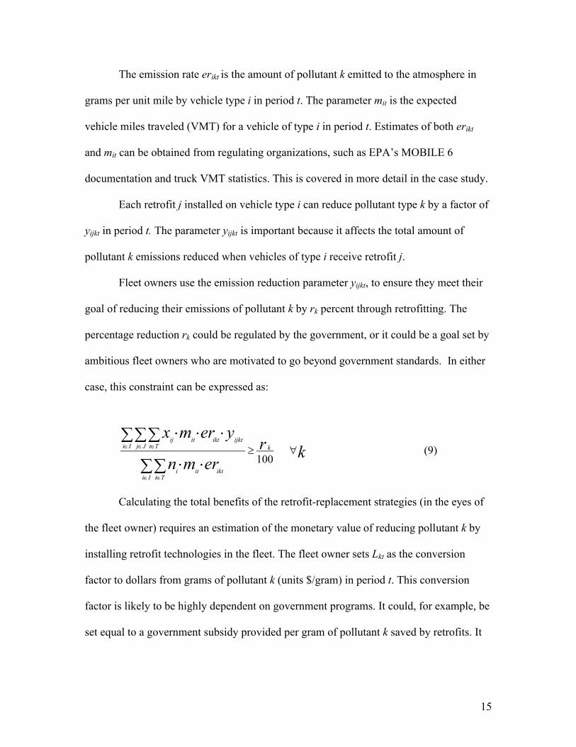
The emission rate erikt is the amount of pollutant k emitted to the atmosphere in

grams per unit mile by vehicle type i in period t. The parameter mit is the expected

vehicle miles traveled (VMT) for a vehicle of type i in period t. Estimates of both erikt

and mit can be obtained from regulating organizations, such as EPA’s MOBILE 6

documentation and truck VMT statistics. This is covered in more detail in the case study.

Each retrofit j installed on vehicle type i can reduce pollutant type k by a factor of

yijkt in period t. The parameter yijkt is important because it affects the total amount of

pollutant k emissions reduced when vehicles of type i receive retrofit j.

Fleet owners use the emission reduction parameter yijkt, to ensure they meet their

goal of reducing their emissions of pollutant k by rk percent through retrofitting. The

percentage reduction rk could be regulated by the government, or it could be a goal set by

ambitious fleet owners who are motivated to go beyond government standards. In either

case, this constraint can be expressed as:

100

ij it ikt ijkti I j J t T k

i it ikti I t T

x m er yr

n m er

k (9)

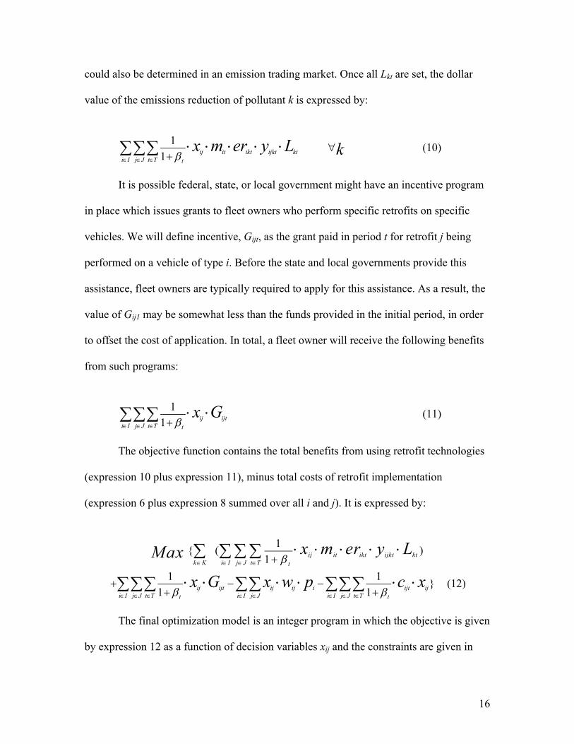
Calculating the total benefits of the retrofit-replacement strategies (in the eyes of

the fleet owner) requires an estimation of the monetary value of reducing pollutant k by

installing retrofit technologies in the fleet. The fleet owner sets Lkt as the conversion

factor to dollars from grams of pollutant k (units $/gram) in period t. This conversion

factor is likely to be highly dependent on government programs. It could, for example, be

set equal to a government subsidy provided per gram of pollutant k saved by retrofits. It

16

could also be determined in an emission trading market. Once all Lkt are set, the dollar

value of the emissions reduction of pollutant k is expressed by:

1

1 ij it ikt ijkt kti I j J t T t

x m er y L k (10)

It is possible federal, state, or local government might have an incentive program

in place which issues grants to fleet owners who perform specific retrofits on specific

vehicles. We will define incentive, Gijt, as the grant paid in period t for retrofit j being

performed on a vehicle of type i. Before the state and local governments provide this

assistance, fleet owners are typically required to apply for this assistance. As a result, the

value of Gij1 may be somewhat less than the funds provided in the initial period, in order

to offset the cost of application. In total, a fleet owner will receive the following benefits

from such programs:

1

1 ij ijti I j J t T t

x G (11)

The objective function contains the total benefits from using retrofit technologies

(expression 10 plus expression 11), minus total costs of retrofit implementation

(expression 6 plus expression 8 summed over all i and j). It is expressed by:

1{ ( )

1 ij it ikt ijkt ktk K i I j J t T t

x m er y LMax

1 1}

1 1ij ijt ij ij i ijt iji I j J t T i I j J i I j J t Tt t

x G x w p c x

(12)

The final optimization model is an integer program in which the objective is given

by expression 12 as a function of decision variables xij and the constraints are given in

17

expressions 1, 2, 3, 4, 5 and 9. The model results indicate the profit maximizing retrofit-

replacement strategy for the selected fleet, retrofit-replacement technologies, regulations,

and incentive programs.

Several constraint types are notably and intentionally absent from this model. For

example, it might appear reasonable to add a budget constraint. Fleet owners are

inevitably bound by budgets, and these budgets influence their decisions. It might seem

logical to require the sum of all costs remain less than some budget. A profit maximizing

fleet owner, however, would be willing to accept higher costs if the benefits compensated

for the costs. Thus, a more appropriate constraint would require that benefits minus costs

are greater than some cutoff. This constraint is effectively already represented by the

objective function. The integer program will return the highest possible objective value

(benefits minus costs). If the result is less than the owner’s cutoff, he or she will know

that there is no feasible solution that meets the cutoff, and must adjust the cutoff or

constraints accordingly. If the result does exceed the cutoff, the fleet owner will know she

has the best feasible solution.

Also apparently absent are the effects of retrofits on fuel consumption. Fuel

consumption is important to fleet owners because it contributes substantially to operating

costs. Fortunately, these effects can actually be included within the current model

framework. In addition to typical diesel pollutants (such as NOx or particulate matter),

the set K could include fuel consumption as a “pollutant.” If fuel consumption is

considered a “pollutant” its “emission rate,” erikt, will be the fuel consumption rate of the

vehicle prior to any retrofits. It makes sense to use units of gallons/mile for fuel, unlike

other pollutants which typically have emissions rates expressed in grams/mile. The

18

constant yijkt would be the fraction reduction in fuel consumption in period t when retrofit

j is applied to vehicle type i. If a retrofit makes a vehicle less fuel efficient, which is

completely possible, yijkt can simply be a negative number. The fleet owner could set Lkt

equal to the average price he or she expects to pay for standard diesel fuel in period t.

Thus, assuming the vehicles use standard fuel both before and after the retrofits, the

monetary benefits of retrofits to fuel consumption will be given by expression 10, where

k is set equal to the index corresponding to fuel in the set K. If a vehicle uses non-

standard fuel, either before or after the retrofit, or both, then obviously Lkt (the expected

price of standard diesel fuel for period t) will not be sufficient for describing fuel costs.

Even in these cases, however, no new variables or parameters need to be added. The

incremental cost of the non-standard fuel can be included by adjusting cijt.

5. Case Study

The purpose of this case study is to demonstrate the types of results that the model

can produce. The particular fleet in question is fictional, as are the government programs.

Nonetheless, they are intended to provide reasonable examples of how this model could

be used and how the results could be interpreted.

Sample Fleet:

Our sample fleet includes 10 HDDV2B trucks from 1989 with 200,000 miles of

use, as well as 20 HDDV8A trucks from 1994 with 400,000 miles of use. The HDDV2B

classification, which is used by the EPA for classifying emissions rates, indicates a light

heavy-duty diesel truck (gross weight between 8,501 and 10,000 lbs) (U.S.

Environmental Protection Agency, 2002a). The HDDV8A classification indicates a

19

heavy heavy-duty diesel truck (gross weight over 60,000 lbs) (U.S. Environmental

Protection Agency, 2002a).

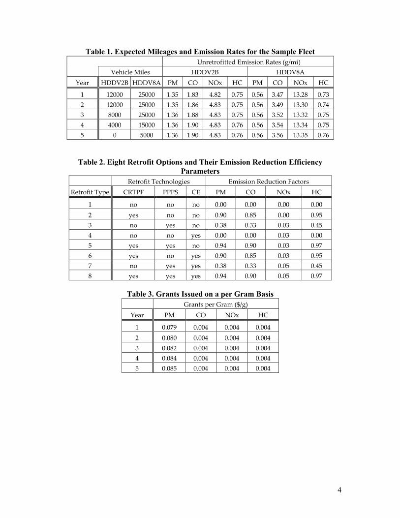
For this example, we will use periods of years. Furthermore, we will say that all

HDDV2B vehicles in the fleet are expected to be in use for another four years, while the

HDDV8A vehicles will be in use for another five years. Expected mileage in each of the

next five years, along with the unretrofitted emissions rates, are given in Table 1.

The Federal Highway Administration (FHWA) publishes estimates of the average

miles traveled by trucks in various uses (U.S. Department of Transportation, 2007), and

our expected mileages fall into the general range of their averages (with the exception of

the last two years of the vehicles’ lives, when their usage is assumed to taper off and drop

below average).

Emissions Rates:

Fleet owners could estimate emissions rates for their vehicles in several different

ways. They could use data provided by the vehicles’ manufacturers and the EPA,

combined with their own knowledge of the environment and mode in which their

vehicles normally operate (altitude, speed, etc) to develop their own unique emission

rates.

Alternatively, fleet owners could use more general averages for a rougher

estimate. It is plausible (even likely) that government agencies would use more general

averages for enforcement purposes, in order to avoid having to trust data provided by the

fleet owners themselves. If the government was using such averages to distribute grants,

it would make sense for fleet owners to use them in their own calculations. Consequently,

we will do just that in this example.

20

We will draw carbon monoxide, nitrogen oxides, and hydrocarbons emission rates

from EPA document M6.HDE.001, which provides emissions rates for use in the EPA’s

mobile emissions model, MOBILE 6.2 (U.S. Environmental Protection Agency, 2002b).

MOBILE 6.2 is currently used by the EPA and represents the state of the practice.

Emission rates in document M6.HDE.001 are in units of grams per brake-horsepower-

hour, however, which we cannot use without a conversion factor. Another EPA

document, M6.HDE.004 (U.S. Environmental Protection Agency, 2002a), provides these

conversion factors to change the units to grams per mile. Conversion factors are

dependent on the vehicle type, as well as the density of the fuel it is using.

Particulate matter emission rates are not described in either of the above

documents. The rates we use are based on values from files that come as a part of the

National Mobile Inventory Model (NMIM), which is an EPA software package including

MOBILE 6.2. We multiply the PM10 emission rates in these files by a factor of 2.3, as

discussed in the EPA’s analysis of the cost effectiveness of particulate matter reducing

retrofits (U.S. Environmental Protection Agency, 2006c). The factor of 2.3 is designed to

compensate for the difference between older engine dynamometer tests and more

accurate chassis dynamometer tests (U.S. Environmental Protection Agency, 2006c).

Even though the factor of 2.3 was developed only from data for HDDV8A trucks, we

apply it to the HDDV2B PM emission rate as well because no comparable factor is

available. The EPA made a similar assumption in applying the factor to vehicles of class

6 and 7 (U.S. Environmental Protection Agency, 2006c). Unlike carbon monoxide,

nitrogen oxides, and hydrocarbons, the HDDV8A particulate matter emission rate is

21

assumed to be constant over the period of analysis. The HDDV2B particulate matter

emission rate increases slowly with vehicle usage.

For this example, the emission rates (g/mile) are listed in Table 1.

[Insert Table 1 about here]

Potential Retrofits:

We will assume that there are three technologies available, all from the EPA’s list

of verified retrofit technologies (U.S. Environmental Protection Agency, 2007e): a

Continuously Regenerating Technology (CRT) Particulate Filter, Platinum Plus Purifier

System (fuel borne catalyst plus diesel oxidation catalyst), and cetane enhancers. Their

individual emission reducing effects on particulate matter, carbon monoxide, nitrogen

oxides, and hydrocarbons are taken directly from the EPA’s list of verified retrofit

technologies, with the mean of the two bounds used where ranges are provided. These

reductions are assumed to be constant with time in the example, but they could be

allowed to change with time. Combinations are assumed to be possible and the reductions

are combined according to the following formula:

1 21 (1 )(1 )T

where φT is the combined reduction and φ1 and φ2 are the reductions due to the individual

technologies. Overall, there are eight retrofit options, all outlined in Table 2.

[Insert Table 2 about here]

Incompatibilities and Mandatory Retrofits:

It is worth noting here that because the HDDV2B trucks were manufactured

before 1994, they are incompatible with the CRT Particulate Filter and therefore cannot

22

receive any retrofits that include it. Otherwise, there are assumed to be no

incompatibilities. We will model this using the required technology constraints. For the

purposes of this example, no technologies will be required. The subset Jri (used in

equation 4) is 1,3,4, and 7 for HDDV2B trucks and 1,2,3,4,5,6,7,8 for HDDV8A trucks.

Grant Programs:

Grants issued on a per gram basis are assumed to be as listed in Table 3.

[Insert Table 3 about here]

The California Air Resources Board’s guidelines for funding emissions reduction

retrofits through the Carl Moyer Program require all potential projects cost no more than

$14300 per “weighted ton of surplus NOx, ROG, and PM 10” where ROG stands for

reactive organic gasses. They defined the “weighted tons of surplus” as the tons of NOx

plus the tons of ROG, plus twenty times the tons of PM. Particulate matter is given more

weight because it has been identified as a toxic air contaminant (California Air Resources

Board, 2005).

The grants per gram are based on this requirement. The value of reducing NOx

HC, or CO, by a ton in the first year is taken to be $14300, while the value of reducing

PM by a ton is taken to be twenty times as much. Correspondingly, the grants per gram

are twenty times as high for PM as for other pollutants.

For two reasons, the grants per gram are not the full “value” of the emissions

reduction, however. First, some funding is being given out in the form of fixed grants,

meaning that if the full “value” was paid in grants per gram, more than the “value” would

be paid in total. Second, the government has limited funds with which to promote

23

retrofits. It is in the interest of the government to pay as little as possible per gram while

still achieving desired reductions. This issue will be explored in more detail in Sensitivity

Analysis section. For now, grants per gram are 25% of the “value” of the emissions

reduction. Any costs beyond these grants are to be covered by fixed grants and the fleet

owner.

In addition, grants per gram are to be increased at a rate of 2% per year, in an

attempt to keep up with inflation. Two percent is used as the rate of inflation because the

Consumer Price Index for all items and all urban consumers increased by roughly 2%

between January 2006 and January 2007 (Bureau of Labor Statistics, 2007).

Fixed grants are assumed to take place only in period 1, and are listed in Table 4,

along with costs and time out of service.

[Insert Table 4 about here]

Retrofit Costs:

The up front costs for CRT Particulate Filters and Platinum Plus Purifier Systems

are loosely based on approximate costs for particulate filters and oxidation catalysts listed

in a letter from the Manufacturers of Emissions Controls Association posted on the EPA

website (U.S. Environmental Protection Agency, 2000).

The cost of the fuel borne catalyst is based on the fuel economies of the trucks

(taken from EPA document M6.HDE.004), the expected mileages for the trucks, and a

price for a fuel borne catalyst posted on the EPA website (U.S. Environmental Protection

Agency, 2006d).

The cost of the cetane enhancer is also based on the fuel economies and expected

mileages of the trucks, in addition to the cost and usage directions of a particular brand of

24

cetane enhancer (AMSOIL, 2007). Table 4 lists the costs of installing these retrofits to

the selected truck classes. No costs are set prohibitively high for the purpose of dealing

with incompatibility.

Opportunity Cost and Required Demand:

The fleet owner does require that the HDDV2B trucks be out of service for a total

time no greater than 300 hours. Similarly, the HDDV8A trucks cannot be out of service

for a total time greater than 200 hours. So long as these absolute constraints are met, it

costs nothing for an HDDV2B truck to be out of service for an hour, but it costs $50 for

each hour a HDDV8A truck is out of service. The time out of service for the different

truck retrofit combinations are listed in Table 4.

Interest Rate:

We will assume the fleet owner expects a yearly return of 7% on investments,

which is a couple percent higher than online savings accounts presently offer. Recall that

βt is defined as the interest rate used to bring dollars from the beginning of period t to the

beginning of period 1. This fleet owner’s beta values are therefore 0, 0.070, 0.145, 0.225,

and 0.311 corresponding to periods 1, 2, 3, 4, and 5 respectively.

Fleet Owner Hesitancy:

The fleet owner is assumed not to set any explicit constraints on the number of

vehicles of a given type to receive a given retrofit. This implies the fleet owner is

prepared to retrofit any number of vehicles with any retrofit, so long as other constraints

are met.

25

Emission Reduction Mandates:

Finally, we need the required reductions in emission levels. We will set the bar

high for particulate matter and carbon monoxide at 50% reduction. We will set a more

moderate goal of 20% reduction for hydrocarbons, and recognizing that nitrogen oxides

are particularly difficult to reduce, not require any reduction.

Computations:

For this case study, the integer program was formulated and run in AMPL. AMPL

is capable of handling integer programs far larger than this case study, and solved the

program almost instantly. Techniques for solving large scale integer programs are beyond

the scope of this paper.

Results:

If we run the model, it tells us the profit maximizing fleet owner will retrofit all

10 of the HDDV2B trucks with Platinum Plus Purifier Systems, and 18 of the 20

HDDV8A trucks with CRT Particulate Filters. From the fleet owner’s perspective, these

retrofits are profitable, and allow the fleet to easily meet the required percentage

reductions. The fleet owner is unable to retrofit the last two trucks because the time

HDDV8A trucks spend out of service would exceed the cap (causing the fleet owner to

be unable to meet required demand).

We can further analyze the results by following the money. For consistency, all

dollars are brought back to the beginning of year 1 using the fleet owner’s chosen interest

rate of 7% per year. The fleet owner received $9,200 in fixed grants ($200 for each of the

10 HDDV2B retrofits, and $400 for each of the 18 HDDV8A retrofits) from the

26

government. In addition, the government paid the fleet owner $101,564 in grants for

reducing emission on a per gram basis. The fleet owner paid about $96,394 for the

retrofits, not including opportunity cost. The opportunity cost was $9,900 ($550 for each

of the 18 HDDV8A retrofits, and nothing for the HDDV2B retrofits) for the time the

vehicles spent out of service. In total, the fleet owner made a profit of just over $4,469

and the government paid $110,764.

The resulting percentage emissions reductions are 67.5% for PM, 72.5% for CO,

0.2% for NOx, and 79% for HC.

Sensitivity Analysis (grants per gram):

When grants per gram were chosen to be 25% of the “value” of the reduction, the

selection of 25% might have seemed somewhat arbitrary. No reasons were given for

selecting 25% as opposed to 50% or 10%. We can examine the implications of our

selection by rerunning the model using different “grant factors.” We will simply define

“grant factor” to be the factor we multiply the “value” of a reduction by to obtain the

grants per gram issued. In the case of 25% it would be .25.

Although it might not be wise to implement a grant factor greater than 1, there is

no reason the model cannot be used to examine results for higher grant factors. The

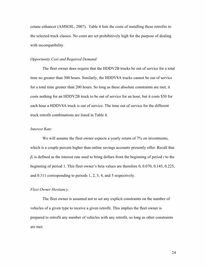
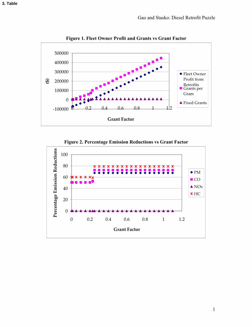
model was rerun with grant factors ranging from 0 to 1.1. The resulting fleet owner profit

and government grants are displayed in Figure 1.

[Insert Figure 1 about here]

27

Clearly, fleet owner profit is closely tied to the grants per gram issued. In this

example, grants per gram make up the vast majority of government grants for all but the

lowest grant factors.

It is apparent from looking at the graph that both grants per gram and profit

generally increase linearly with the grant factor. There is, however, an exception between

grant factors of .2 and .25. On either side of this gap, the behavior is linear, albeit with

different slopes. This result is a symptom of the fact that between grant factors of .2 and

.25 the optimal retrofit package changes. Outside of this range, it does not. If the optimal

retrofit package does not change, the only change in profit is from the increasing grants

per gram for the same retrofits.

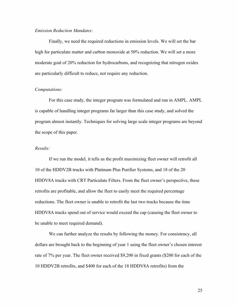
Changes in optimal retrofit packages are the source of changes in emission

reductions. Consequently, in Figure 2 we see no changes in emission reductions outside

of the region between .2 and .25.

[Insert Figure 2 about here]

With these two graphs in mind, it seems to make little sense to use a grant factor

much higher than .25 in this case. The fleet owner is already making a small profit off the

retrofits, and higher grants per gram will not lead to any more emissions reductions.

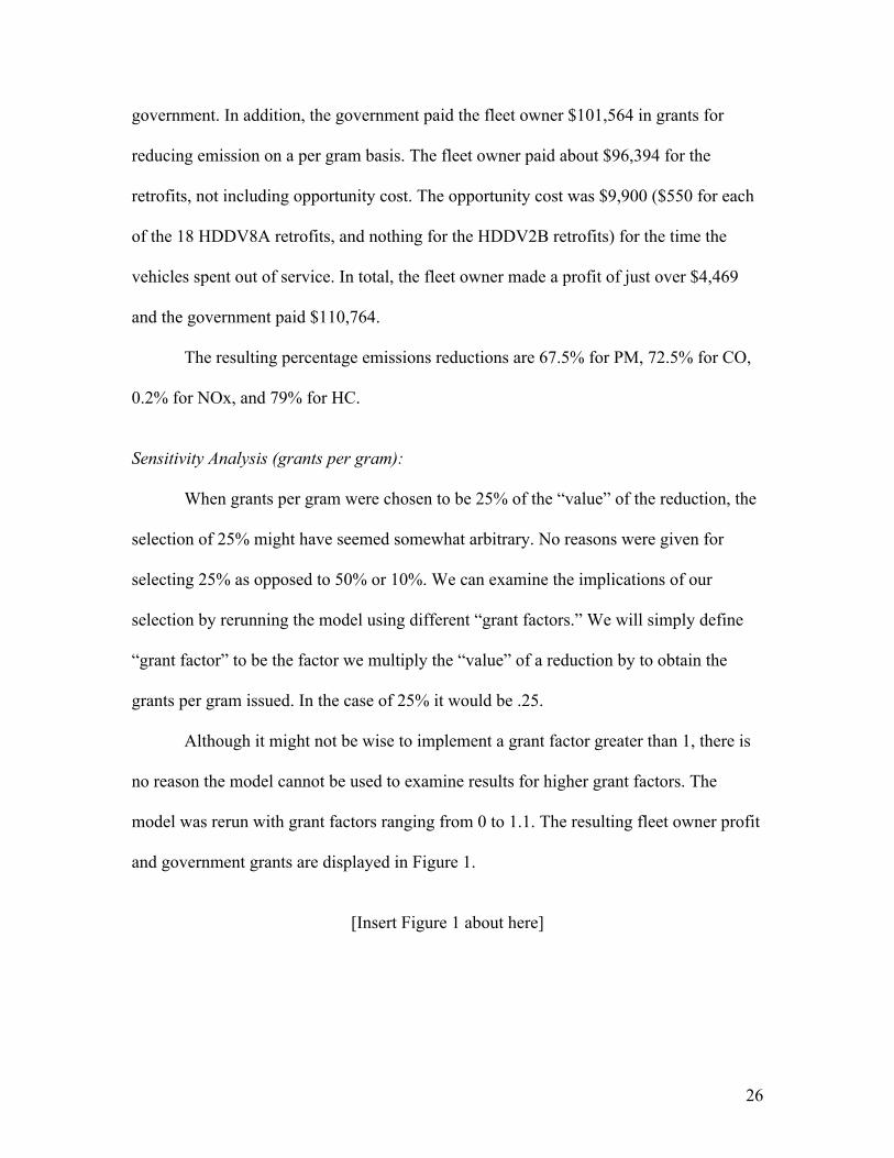
In our example, it would be reasonable to say that one of the principle goals of the

government is to achieve the greatest reductions possible per dollar it spends. We can

quantify this by using the weighted sum of the mass reductions divided by the total grants

(where we weight particulate matter emissions with 20 and all other emissions with 1 as

discussed in the Grant Programs section). We can calculate this measure of success for

our range of emission factors (Figure 3).

28

[Insert Figure 3 about here]

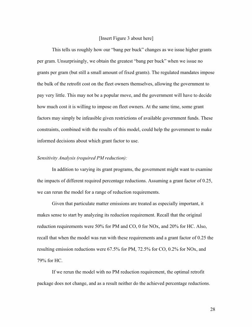
This tells us roughly how our “bang per buck” changes as we issue higher grants

per gram. Unsurprisingly, we obtain the greatest “bang per buck” when we issue no

grants per gram (but still a small amount of fixed grants). The regulated mandates impose

the bulk of the retrofit cost on the fleet owners themselves, allowing the government to

pay very little. This may not be a popular move, and the government will have to decide

how much cost it is willing to impose on fleet owners. At the same time, some grant

factors may simply be infeasible given restrictions of available government funds. These

constraints, combined with the results of this model, could help the government to make

informed decisions about which grant factor to use.

Sensitivity Analysis (required PM reduction):

In addition to varying its grant programs, the government might want to examine

the impacts of different required percentage reductions. Assuming a grant factor of 0.25,

we can rerun the model for a range of reduction requirements.

Given that particulate matter emissions are treated as especially important, it

makes sense to start by analyzing its reduction requirement. Recall that the original

reduction requirements were 50% for PM and CO, 0 for NOx, and 20% for HC. Also,

recall that when the model was run with these requirements and a grant factor of 0.25 the

resulting emission reductions were 67.5% for PM, 72.5% for CO, 0.2% for NOx, and

79% for HC.

If we rerun the model with no PM reduction requirement, the optimal retrofit

package does not change, and as a result neither do the achieved percentage reductions.

29

The requirement was not binding because the retrofits were profitable. So long as the

requirement for PM reduction is less than or equal to 67.5 it has no effect on the optimal

retrofit package for this fleet.

If we rerun the model with a PM reduction requirement of 68% we find that the

problem is infeasible. We weighted PM reductions very heavily when we assigned grants

per gram. This drove the fleet owner to select retrofits which reduce PM. In particular, it

turned out that the retrofit package which achieved the greatest reduction in PM was in

fact the most profitable retrofit package. As a result, PM reduction requirements serve no

purpose in this example.

Sensitivity Analysis (required NOx reduction):

Nitrogen Oxides were given far lower priority than particulate matter when

assigning grants, and no requirement was set for their reduction. It would be reasonable

to ask what the effect would be of requiring just a small reduction in NOx emissions.

In order for such a requirement to have any effect, it would have to exceed the

achieved reductions when no requirement was imposed (.2 percent). At the same time, a

reduction in NOx emissions of 4.2 percent or greater is infeasible in our example. The

retrofit packages with the highest NOx reductions (7 and 8) reduce NOx by 5 percent, but

they cannot be applied to all vehicles without violating other reduction constraints.

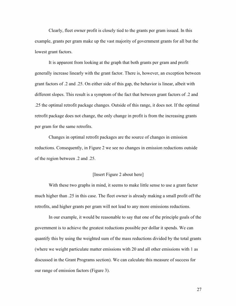
Fleet owner profit in the context of several possible NOx reduction requirements

is plotted in Figure 4.

[Insert Figure 4 about here]

30

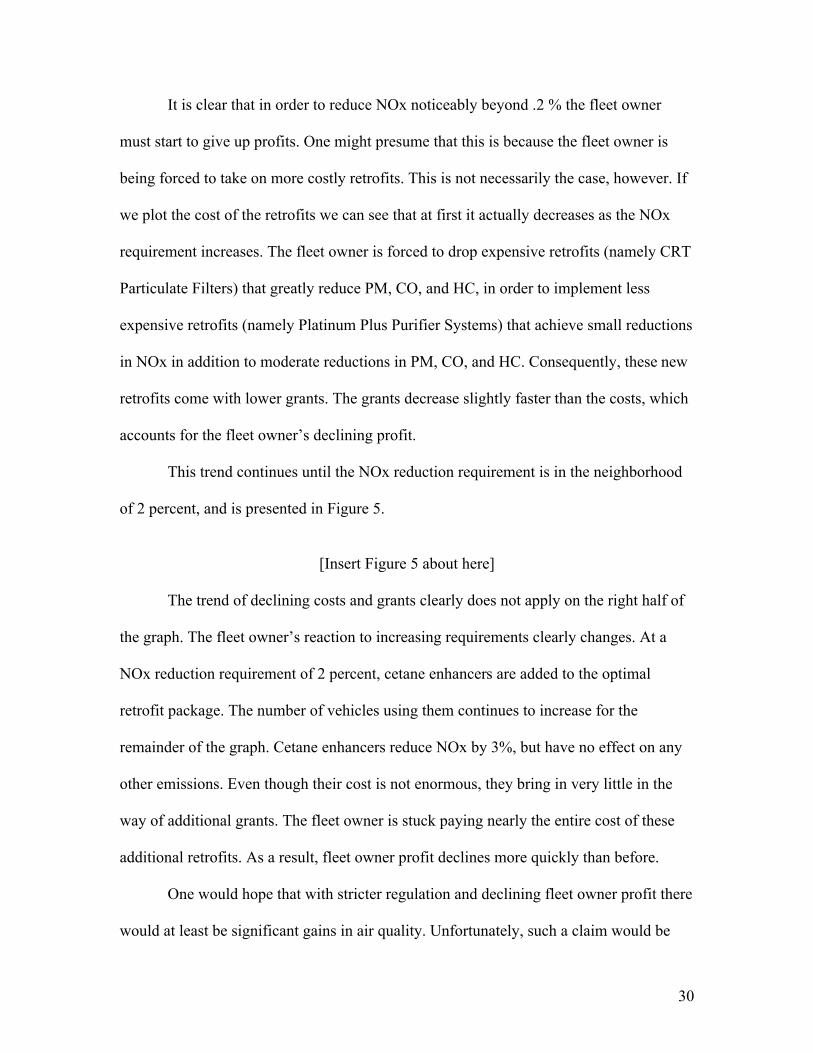
It is clear that in order to reduce NOx noticeably beyond .2 % the fleet owner

must start to give up profits. One might presume that this is because the fleet owner is

being forced to take on more costly retrofits. This is not necessarily the case, however. If

we plot the cost of the retrofits we can see that at first it actually decreases as the NOx

requirement increases. The fleet owner is forced to drop expensive retrofits (namely CRT

Particulate Filters) that greatly reduce PM, CO, and HC, in order to implement less

expensive retrofits (namely Platinum Plus Purifier Systems) that achieve small reductions

in NOx in addition to moderate reductions in PM, CO, and HC. Consequently, these new

retrofits come with lower grants. The grants decrease slightly faster than the costs, which

accounts for the fleet owner’s declining profit.

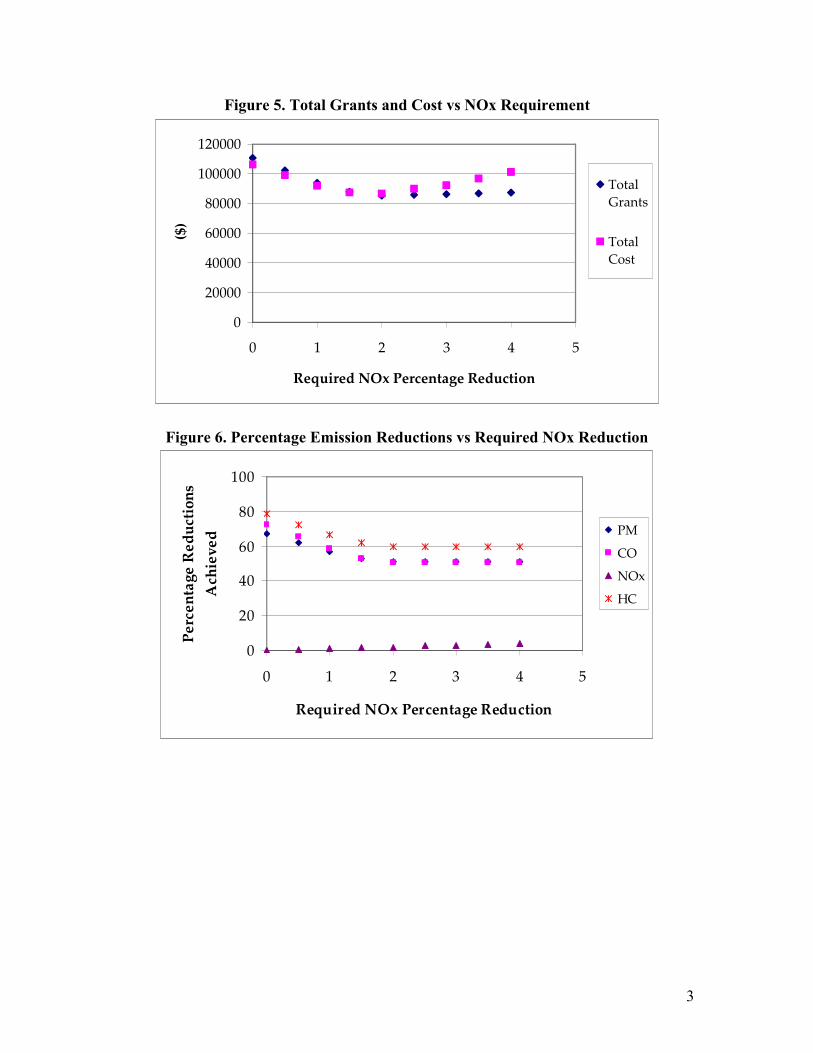
This trend continues until the NOx reduction requirement is in the neighborhood

of 2 percent, and is presented in Figure 5.

[Insert Figure 5 about here]

The trend of declining costs and grants clearly does not apply on the right half of

the graph. The fleet owner’s reaction to increasing requirements clearly changes. At a

NOx reduction requirement of 2 percent, cetane enhancers are added to the optimal

retrofit package. The number of vehicles using them continues to increase for the

remainder of the graph. Cetane enhancers reduce NOx by 3%, but have no effect on any

other emissions. Even though their cost is not enormous, they bring in very little in the

way of additional grants. The fleet owner is stuck paying nearly the entire cost of these

additional retrofits. As a result, fleet owner profit declines more quickly than before.

One would hope that with stricter regulation and declining fleet owner profit there

would at least be significant gains in air quality. Unfortunately, such a claim would be

31

debatable at best. When the fleet owner swapped retrofits in order to meet the NOx

requirement, substantial improvements in PM, CO, and HC emissions were lost. The

additional NOx reductions are barely noticeable in comparison (Figure 6).

[Insert Figure 6 about here]

In order for a NOx reduction requirement to make sense in this case, NOx

emissions would have to be viewed as far more important than PM, CO, and HC.

6. Conclusions

The types of results produced by this integer programming model, such as those

in the case study, are relevant to two principle groups of decision makers: diesel fleet

owners looking to select pollution control retrofits, and government officials looking to

predict fleet owner behavior.

For a fleet owner, the model provides guidance on how to maximize profits

through the selection of retrofits for his or her particular fleet. The model accounts for a

considerable range of potential regulatory and incentive environments, as well as

constraints imposed by the business environment (such as needing to meet specific

demands). Furthermore, the fleet owner can benefit from knowing how his or her profit

would change if regulations were altered. Such knowledge could inform a targeted

lobbying campaign.

From the government’s perspective, this model can serve as a tool to predict how

a particular fleet might respond to government programs designed to encourage retrofits.

As the case study revealed, tighter regulation does not always necessarily yield cleaner

air. Regulations can cause enhancements of some aspects of air quality while causing

32

degradations of others. A model that predicts such results can help policy makers select

the appropriate tradeoffs.

There are numerous directions for future research in this field. Several

assumptions could be relaxed. The remaining miles for vehicles could be treated as a

variable as opposed to a constant. Retrofits need not all take place at the same period in

time. A second level could be added to the optimization problem to represent the

behavior of a regulatory agency supervising multiple fleets. An emissions market could

be modeled.

Given the severe impacts of diesel emissions, and the immediate nature of the

problem, such continued research has the potential to provide substantial benefits to

society.

Acknowledgements

The authors would like to thank the dedicated staff at the EPA, especially David

Brzezinski and Larry Landman, who took the time to provide thorough documentation

and to answer questions on EPA models and research. We are also grateful to Joanne Lee

for her help in the early preparation of the study. This research was partly supported by a

mini paper grant from University Transportation Research Center, Region II.

Appendix A: Grant Types

Given that the remaining mileages are fixed and known for all vehicles, one might

argue that grants per gram could effectively be included in the “fixed” grants Gijt. This is

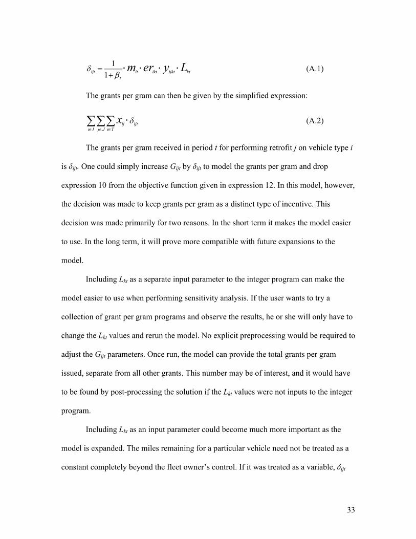
completely true. Recall that the grants per gram were given by expression 10. Let δijt be

defined by:

33

1

1ijt it ikt ijkt ktt

m er y L

(A.1)

The grants per gram can then be given by the simplified expression:

ij ijti I j J t T

x

(A.2)

The grants per gram received in period t for performing retrofit j on vehicle type i

is δijt. One could simply increase Gijt by δijt to model the grants per gram and drop

expression 10 from the objective function given in expression 12. In this model, however,

the decision was made to keep grants per gram as a distinct type of incentive. This

decision was made primarily for two reasons. In the short term it makes the model easier

to use. In the long term, it will prove more compatible with future expansions to the

model.

Including Lkt as a separate input parameter to the integer program can make the

model easier to use when performing sensitivity analysis. If the user wants to try a

collection of grant per gram programs and observe the results, he or she will only have to

change the Lkt values and rerun the model. No explicit preprocessing would be required to

adjust the Gijt parameters. Once run, the model can provide the total grants per gram

issued, separate from all other grants. This number may be of interest, and it would have

to be found by post-processing the solution if the Lkt values were not inputs to the integer

program.

Including Lkt as an input parameter could become much more important as the

model is expanded. The miles remaining for a particular vehicle need not be treated as a

constant completely beyond the fleet owner’s control. If it was treated as a variable, δijt

34

would no longer be a constant and could not be added to Gijt as one. Also, the Lkt values

themselves could be treated as variables in an emissions market. This would cause δijt to

become a variable as well.

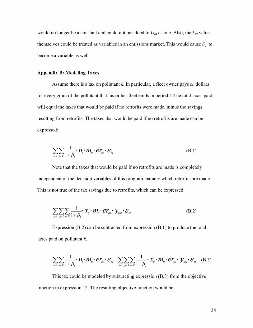
Appendix B: Modeling Taxes

Assume there is a tax on pollutant k. In particular, a fleet owner pays εkt dollars

for every gram of the pollutant that his or her fleet emits in period t. The total taxes paid

will equal the taxes that would be paid if no retrofits were made, minus the savings

resulting from retrofits. The taxes that would be paid if no retrofits are made can be

expressed:

1

1 i it ikt kti I t T t

n m er

(B.1)

Note that the taxes that would be paid if no retrofits are made is completely

independent of the decision variables of this program, namely which retrofits are made.

This is not true of the tax savings due to retrofits, which can be expressed:

1

1 ij it ikt ijkt kti I j J t T t

x m er y

(B.2)

Expression (B.2) can be subtracted from expression (B.1) to produce the total

taxes paid on pollutant k.

1 1

1 1i it ikt kt ij it ikt ijkt kti I t T i I j J t Tt t

n m er x m er y

(B.3)

This tax could be modeled by subtracting expression (B.3) from the objective

function in expression 12. The resulting objective function would be:

35

1{ ( )

1 ij it ikt ijkt ktk K i I j J t T t

x m er y LMax

1 1

1 1ij ijt ij ij i ijt iji I j J t T i I j J i I j J t Tt t

x G x w p c x

1 1}

1 1i it ikt kt ij it ikt ijkt kti I t T i I j J t Tt t

n m er x m er y

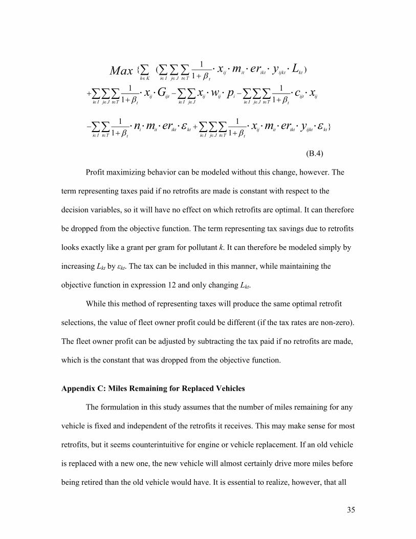
(B.4)

Profit maximizing behavior can be modeled without this change, however. The

term representing taxes paid if no retrofits are made is constant with respect to the

decision variables, so it will have no effect on which retrofits are optimal. It can therefore

be dropped from the objective function. The term representing tax savings due to retrofits

looks exactly like a grant per gram for pollutant k. It can therefore be modeled simply by

increasing Lkt by εkt. The tax can be included in this manner, while maintaining the

objective function in expression 12 and only changing Lkt.

While this method of representing taxes will produce the same optimal retrofit

selections, the value of fleet owner profit could be different (if the tax rates are non-zero).

The fleet owner profit can be adjusted by subtracting the tax paid if no retrofits are made,

which is the constant that was dropped from the objective function.

Appendix C: Miles Remaining for Replaced Vehicles

The formulation in this study assumes that the number of miles remaining for any

vehicle is fixed and independent of the retrofits it receives. This may make sense for most

retrofits, but it seems counterintuitive for engine or vehicle replacement. If an old vehicle

is replaced with a new one, the new vehicle will almost certainly drive more miles before

being retired than the old vehicle would have. It is essential to realize, however, that all

36

the miles driven by the new vehicle need not provide emission reductions. Initially, the

replacement vehicle is driving miles that the old vehicle would have driven, and for these

miles our model calculates the reductions. Afterwards, the replacement vehicle is driving

miles that another, possibly different, new vehicle would have driven. Furthermore, the

decision to replace a vehicle early could quite possibly influence when other vehicles are

retired further down the line. Quantifying the emission reductions resulting from these

changes is extremely difficult, given the level of uncertainty regarding future emissions

standards. For this reason, only the pollution reductions from the miles that the original

old vehicle would have driven are used in calculations.

Appendix D: Implicit Representation of Incompatibilities

As previously discussed, there may be some occasions when vehicle type i is

incompatible with retrofit j. This can be dealt with explicitly in either the upper bounds in

expression 2 or the required technologies constraints in expression 4. Alternatively, if

there are no required technologies or other needs for upper bounds, the fleet owner may

wish to remove constraint 4 and the upper bounds in constraint 2 (leaving the non-

negativity constraints) to simplify the problem. This can be accomplished while

implicitly forcing xij to remain zero for incompatible pairings. Set cijt to high positive

numbers for all t while setting yijkt equal to zero for all k and t. By looking at the objective

function, one can discern that if yijkt is zero for all k and t, and both wij and pi are non-

negative, the only benefit corresponding to xij will be Gijt. So long as cijt is set to be

greater than Gijt for all t, implementation of the retrofit j on vehicle type i will only

decrease the objective function. Implementation will not help the fleet owner to meet any

requirements on emission reductions (due to yijkt being 0 for all k and t) or reduce the time

37

out of service (due to wij being non-negative). So long as there exists a “do nothing”

retrofit option with no costs, benefits, or time spent out of service, retrofit j will never be

selected for vehicle type i. With this technique, we need not explicitly formulate the

incompatibilities. This helps to reduce the complexity of the model.

38

References

AMSOIL, 2007. Cetane boost diesel fuel additive (ACB). Retrieved 28 May 2007, from http://www.amsoil.com/storefront/acb.aspx

Bureau of Labor Statistics, 2007. Consumer price index – all urban consumers. Retrieved 28 May 2007, from http://data.bls.gov/cgi-bin/surveymost?cu

California Air Resources Board, 2005. The Carl Moyer program guidelines part IV: appendices. Retrieved 28 May 2007, from http://www.arb.ca.gov/msprog/moyer/guidelines/2005_Carl_Moyer_Guidelines_Part4.pdf

California Air Resources Board, 2006. Carl Moyer program guidelines. Retrieved 28 May 2007, from http://www.arb.ca.gov/msprog/moyer/guidelines/current.htm

California Air Resources Board, 2007a. Carl Moyer Memorial air quality standardsattainment program. Retrieved 28 May 2007, from http://www.arb.ca.gov/msprog/moyer/moyer.htm

California Air Resources Board, 2007b. Currently verified technologies. Retrieved 28 May 2007, from http://www.arb.ca.gov/diesel/verdev/vt/cvt.htm

Charnes, A., Cooper, W. W., Harrald, J., Karwan, K. R., Wallace, W. A., 1976. A goal interval programming model for resource allocation in a marine environmental protection program. Journal of Environmental Economics and Management 3, 347-362.

Clean Air Task Force, 2005. Diesel health in America: the lingering threat. Clean Air Task Force, Boston.

Gürdal, Z., Haftka, R. T., Hajela, P., 1999. Design and optimization of laminated composite materials, Wiley-Interscience, New Jersey.

Janic, M., 2003. Modelling operational, economic, and environmental performance of an air transport network. Transportation Research D 8, 415-432.

Marino, A. M., Sicilian, J., 1988. The incentive for conservation investment in regulated utilities. Journal of Environmental Economics and Management 15, 173-188.

Marsten, R. E., Muller, M.R., 1980. A mixed-integer programming approach to air cargo fleet planning. Management Science 26, 1096-1107.

National Research Council (NRC), 2004. Air quality management in the United States, National Academy Press, Washington, D.C.

39

Schipper, L., 2005. Cleaner buses for Mexico City: from talk to reality. Transportation Research Board Annual Meeting CD, 2006, Washington DC.

U.S. Department of Transportation: Federal Highway Administration, 2007. 2006 status of the nation's highways, bridges, and transit: conditions and performance. Retrieved 4 June 2007, fromhttp://www.fhwa.dot.gov/policy/2006cpr/chap14.htm

U.S. Environmental Protection Agency, 2000. MECA independent cost survey for emission control retrofit technologies. Manufacturers of Emissions Controls Association. Retrieved 28 May 2007, from http://www.epa.gov/otaq/retrofit/documents/meca1.pdf

U.S. Environmental Protection Agency, 2002a. Update heavy-duty engine emission conversion factors for MOBILE6: analysis of BSFCs and calculation of heavy-duty emission conversion factors: M6.HDE.004, USEPA #420-R-02-005. Retrieved 28 May 2007, fromhttp://www.epa.gov/otaq/models/mobile6/r02005.pdf

U.S. Environmental Protection Agency, 2002b. Update of heavy-duty emission levels (Model Years 1988-2004) for use in MOBILE6: M6.HDE.001, USEPA #420-R-02-018. Retrieved 28 May 2007, from http://www.epa.gov/otaq/models/mobile6/r02018.pdf

U.S. Environmental Protection Agency, 2003. Diesel exhaust in the United States, USEPA #420-F-03-022. Retrieved 28 May 2007, from http://www.epa.gov/otaq/retrofit/documents/420f03022.pdf

U.S. Environmental Protection Agency, 2006a. Voluntary diesel retrofit program: fleet assessment. Retrieved 28 May 2007, from http://www.epa.gov/otaq/retrofit/retrofitfleet.htm

U.S. Environmental Protection Agency, 2006b. Modeling and inventories: National Mobile Inventory Model (NMIM). Retrieved 28 May 2007, from http://www.epa.gov/otaq/nmim.htm

U.S. Environmental Protection Agency, 2006c. Diesel retrofit technology: an analysis of the cost-effectiveness of reducing particulate matter emissions from heavy duty diesel engines through retrofits, USEPA #420-S-06-002. Retrieved 28 May 2007, from http://www.epa.gov/cleandiesel/documents/420s06002.pdf

U.S. Environmental Protection Agency, 2006d. Voluntary diesel retrofit program: technical summary. Retrieved 28 May 2007, from http://www.epa.gov/otaq/retrofit/retropotentialtech.htm

40

U.S. Environmental Protection Agency, 2006e. Diesel retrofits: quantifying and using their benefits in SIPs and conformity--guidance for state and local air and transportation agencies. Retrieved 28 May 2007, from http://www.epa.gov/otaq/stateresources/transconf/policy/420b06005.pdf.

U.S. Environmental Protection Agency, 2007a. National clean diesel campaign. Retrieved 28 May 2007, from http://www.epa.gov/cleandiesel/

U.S. Environmental Protection Agency, 2007b. U.S. greenhouse gas inventory executive summary, USEPA #430-R-07-002. Retrieved 28 May 2007, from http://www.epa.gov/climatechange/emissions/downloads06/07ES.pdf

U.S. Environmental Protection Agency, 2007c. Eight-hour ground-level ozone designations. Retrieved 28 May 2007, from http://www.epa.gov/oar/oaqps/glo/designations/statedesig.htm

U.S. Environmental Protection Agency, 2007d. Voluntary diesel retrofit program: diesel emissions. Retrieved 28 May 2007, from http://www.epa.gov/otaq/retrofit/overdieselemissions.htm

U.S. Environmental Protection Agency, 2007e. Voluntary diesel retrofit program: verified products. Retrieved 28 May 2007, from http://www.epa.gov/otaq/retrofit/retroverifiedlist.htm

Vollebergh, H. R. J., De Vries, J. L., Koutstaal, P. R., 1997. Hybrid carbon incentive mechanisms and political acceptability. Environmental and Resource Economics 9, 43-63.

Zodrow, G., 1992. Grandfather rules and the theory of optimal tax reform. Journal of Public Economics 49, 163-190.

Gao and Stasko: Diesel Retrofit Puzzle

1

Figure 1. Fleet Owner Profit and Grants vs Grant Factor

-100000

0

100000

200000

300000

400000

500000

0 0.2 0.4 0.6 0.8 1 1.2

Grant Factor

($)

Fleet OwnerProfit fromRetrofitsGrants perGram

Fixed Grants

Figure 2. Percentage Emission Reductions vs Grant Factor

0

20

40

60

80

100

0 0.2 0.4 0.6 0.8 1 1.2

Grant Factor

Perc

enta

ge E

mis

sion

Red

uctio

ns

PM

CO

NOx

HC

3. Table

2

Figure 3. Weighted Emissions Reduction/Total Grants vs Grant Factor

00.5

1

1.52

2.53

3.5

0 0.2 0.4 0.6 0.8 1 1.2

Grant Factor

Wei

ghte

d Em

issi

ons

Red

uctio

n/To

tal G

rant

s (k

g/$)

Figure 4. Fleet Owner Profit vs NOx Requirement

-15000

-10000

-5000

0

5000

10000

0 1 2 3 4 5

Required NOx Percentage Reduction

Flee

t Ow

ner P

rofi

t fro

m R

etro

fits

($

)

3

Figure 5. Total Grants and Cost vs NOx Requirement

0

20000

40000

60000

80000

100000

120000

0 1 2 3 4 5

Required NOx Percentage Reduction

($)

TotalGrants

TotalCost

Figure 6. Percentage Emission Reductions vs Required NOx Reduction

0

20

40

60

80

100

0 1 2 3 4 5

Required NOx Percentage Reduction

Perc

enta

ge R

educ

tions

A

chie

ved PM

CO

NOx

HC

4

Table 1. Expected Mileages and Emission Rates for the Sample Fleet Unretrofitted Emission Rates (g/mi)

Vehicle Miles HDDV2B HDDV8AYear HDDV2B HDDV8A PM CO NOx HC PM CO NOx HC

1 12000 25000 1.35 1.83 4.82 0.75 0.56 3.47 13.28 0.732 12000 25000 1.35 1.86 4.83 0.75 0.56 3.49 13.30 0.743 8000 25000 1.36 1.88 4.83 0.75 0.56 3.52 13.32 0.754 4000 15000 1.36 1.90 4.83 0.76 0.56 3.54 13.34 0.755 0 5000 1.36 1.90 4.83 0.76 0.56 3.56 13.35 0.76

Table 2. Eight Retrofit Options and Their Emission Reduction Efficiency Parameters

Retrofit Technologies Emission Reduction FactorsRetrofit Type CRTPF PPPS CE PM CO NOx HC

1 no no no 0.00 0.00 0.00 0.002 yes no no 0.90 0.85 0.00 0.953 no yes no 0.38 0.33 0.03 0.454 no no yes 0.00 0.00 0.03 0.005 yes yes no 0.94 0.90 0.03 0.976 yes no yes 0.90 0.85 0.03 0.957 no yes yes 0.38 0.33 0.05 0.458 yes yes yes 0.94 0.90 0.05 0.97

Table 3. Grants Issued on a per Gram BasisGrants per Gram ($/g)

Year PM CO NOx HC

1 0.079 0.004 0.004 0.0042 0.080 0.004 0.004 0.0043 0.082 0.004 0.004 0.0044 0.084 0.004 0.004 0.0045 0.085 0.004 0.004 0.004

5

Table 4. Fixed Grants, Costs, and Time out of Service Costs Beyond Opportunity Cost ($)

Retrofit Type Year 1 Year 2 Year 3 Year 4 Year 5Out of Service

(hours)Fixed Grants in Year 1 ($)

1 0 0 0 0 0 0 02 4500 0 0 0 0 12 03 1450 50 33 17 0 10 2004 60 60 40 20 0 0 05 5950 50 33 17 0 21 06 4560 60 40 20 0 12 07 1510 110 73 37 0 10 200

HD

DV

2B

8 6010 110 73 37 0 21 01 0 0 0 0 0 0 02 4500 0 0 0 0 11 4003 1694 194 194 116 39 10 2504 233 233 233 140 47 0 05 6194 194 194 116 39 20 6506 4733 233 233 140 47 11 4007 1927 427 427 256 86 10 250

HD

DV

8A

8 6427 427 427 256 86 20 650