THE RESPONSE OF DRUG EXPENDITURE TONON-LINEAR CONTRACT DESIGN: EVIDENCE FROM

MEDICARE PART D�

Liran EinavAmy FinkelsteinPaul Schrimpf

Abstract. We study the demand response to non-linear price schedules using dataon insurance contracts and prescription drug purchases in Medicare Part D. We exploit

the kink in individuals�budget set created by the famous �donut hole,�where insurance

becomes discontinuously much less generous on the margin, to provide descriptive evi-

dence of the drug purchase response to a price increase. We then specify and estimate

a simple dynamic model of drug use that allows us to quantify the spending response

along the entire non-linear budget set. We use the model for counterfactual analysis of

the increase in spending from ��lling�the donut hole, as will be required by 2020 under

the A¤ordable Care Act. In our baseline model, which considers spending decisions

within a single year, we estimate that ��lling�the donut hole will increase annual drug

spending by about $150, or about 8 percent. About one-quarter of this spending in-

crease re�ects �anticipatory�behavior, coming from bene�ciaries whose spending prior

to the policy change would leave them short of reaching the donut hole. We also present

descriptive evidence of cross-year substitution of spending by individuals who reach the

kink, which motivates a simple extension to our baseline model that allows �in a highly

stylized way �for individuals to engage in such cross year substitution. Our estimates

from this extension suggest that a large share of the $150 drug spending increase could

be attributed to cross-year substitution, and the net increase could be as little as $45

per year.

�We thank Larry Katz, Elhanan Helpman, �ve anonymous referees, Jason Abaluck, Raj Chetty, John Friedman,

Ben Handel, Nathan Hendren, Day Manoli, Maria Polyakova, and many seminar participants for useful comments

and helpful discussions, and Allyson Barnett, Ray Kluender, and Belinda Tang for extraordinary research assistance.

We gratefully acknowledge support from the NIA (R01 AG032449).

I. Introduction

A classic empirical exercise is to study how demand responds to price. Many settings, from cell

phones to electricity to health insurance, give rise to non-linear pricing schedules. These o¤er both

challenges and opportunities for empirical estimation, while at the same time raising interesting

conceptual questions regarding the nature of the demand response.

We study the demand response to non-linear contracts, and its implications for the impact

of counterfactual contract design, in a particular context: the Medicare Part D prescription drug

bene�t. The 2006 introduction of Medicare Part D was by far the most important bene�t expansion

in Medicare�s nearly half-century of existence. In 2013, about 37 million people received Part

D coverage (Kaiser Family Foundation 2014). We analyze the response of drug expenditures to

insurance contract design using detailed micro data on insurance contracts and prescription drug

purchases from a 20% random sample of Medicare Part D bene�ciaries from 2007 to 2009. Section

II describes the data and institutional setting in more detail.

Figure I illustrates the highly non-linear nature of the Part D contracts; it shows the 2008

government-de�ned standard bene�t design. In this contract, the individual initially pays for all

expenses out of pocket, until she has spent $275, at which point she pays only 25% of subsequent

drug expenditures until her total drug spending reaches $2,510. At this point the individual enters

the famed �donut hole,�or the �gap,�within which she must once again pay for all expenses out

of pocket, until total drug expenditures reach $5,726, the amount at which catastrophic coverage

sets in and the marginal out-of-pocket price of additional spending drops substantially, to about

7%. Individuals may buy plans that are actuarially equivalent to, or have more coverage than the

standard plan, so that the exact contract design varies across individuals. Nonetheless, a common

feature of these plans is the existence of substantial non-linearities that are similar to the standard

coverage we have just described. For example, in our sample a bene�ciary entering the coverage

gap at the �donut hole�experiences, on average, a price increase of almost 60 cents for every dollar

of total spending.

Motivated by these contract features, we begin in Section III by exploiting the kink in the

individual�s budget set created by the donut hole to provide descriptive evidence on the nature

of the drug purchase response to the drug price increase at the kink. We document signi�cant

�excess mass,�or �bunching�of annual spending levels around the kink. This is visually apparent

in even the basic distribution of annual drug spending in any given year, as shown in Figure II for

2008. The behavioral response appears to grow over time, which may re�ect a �learning� e¤ect

(by individuals or pharmacists) about the presence of the gap in the new program; it also tends

to be larger for healthier individuals. Using the detailed data on the timing of claims, we also

show a sharp decline in the propensity to claim toward the end of the year for those individuals

whose spending is near the kink. This decline is concentrated later in the year but is also visible at

earlier months in the year; this is consistent with individuals updating over the course of the year

about their expected end-of-year price, and having a positive discount factor. The decline in drug

purchases for individuals near the kink is substantially more pronounced for branded than generic

1

drugs.

The descriptive results provide qualitative evidence of the extent and nature of the drug purchase

response to the insurance contract. To quantify this response and use it for counterfactual analysis

of behavior under other contracts requires us to develop and estimate a model of individual behavior.

Section IV presents therefore a simple, dynamic model of an optimizing agent�s prescription drug

utilization decisions within a single year when faced with a speci�c, non-linear contract design. The

model illustrates the key economic and statistical objects that determine the expenditure response

to the contract. The �rst key object is the distribution of health-related events, which determine

the set of potential prescription drug expenditures, and which we allow to vary across observable

and unobservable patient characteristics, including patient health. The second is the �primitive�

price elasticity that captures the individual�s willingness to trade o¤ health and income, which we

also allow to be heterogeneous across observable and unobservable patient characteristics. The

third object is the extent to which individuals respond to the dynamic incentives associated with

the non-linear contract. We parameterize the model and estimate it using method of moments,

relying on the descriptive patterns in the data described earlier, as well as additional features of

the data and modeling assumptions. The estimated model �ts the data reasonably well.

Section V presents the main results. We illustrate the demand response to non-linear contract

design through analysis of a speci�c, policy-relevant counterfactual contract: the requirement in the

2010 A¤ordable Care Act (ACA) that, e¤ective in 2020, the standard (i.e. minimal) bene�t plan

eliminate the donut hole, providing the same 25% consumer cost-sharing from the deductible to the

catastrophic limit (compared to the 100% consumer cost sharing in the gap in the original design).

We estimate that this ACA policy of ��lling the gap�will increase total, annual drug spending

by $150 per bene�ciary (or about 8%), and will increase Medicare drug spending by substantially

more (by $260 per bene�ciary, or about 25%). By comparison, holding behavior constant, we

estimate the �mechanical� consequence of �lling the gap would be to increase average Medicare

drug spending by only about 60% of our estimated e¤ect.

The results also illustrate some of the subtle, distributional e¤ects that non-linear contracts

can produce. For example, we �nd that somewhat counter-intuitively, �lling the gap provides less

coverage on the margin to some individuals, causing them to decrease their spending. We also

show that �lling the gap changes spending behavior for individuals far from the gap; we estimate

that about one-quarter of the $150 per-bene�ciary increase in annual drug spending from �lling the

gap comes from �anticipatory�responses by individuals whose annual spending prior to the policy

change would have been below the gap.

In the �nal section of the paper, we consider yet another implication of non-linear contracts:

potential incentives for cross-year substitution. We provide descriptive evidence that some, but

not all of the decline in purchasing for individuals who reach the kink re�ects the postponement

of purchases to the beginning of the subsequent year. To quantitatively assess the importance

of this cross-year substitution for our main results, we provide a simple extension to the baseline

model that allows �in a highly stylized way �for individuals to engage in cross-year substitution.

The results suggest that up to two thirds of the annual spending increase from �lling the gap may

2

be explained by a decline in substitution of purchases to the subsequent year, rather than a net

increase in spending over a longer-than-annual horizon; as a result, the net increase in spending

may be as little as $45 per year.

Our �ndings have several implications for future empirical work on �moral hazard� (that is,

spending) e¤ects of health insurance contracts. Most of this literature has focused on characterizing

the spending e¤ect of a health insurance contract with respect to a given single price despite the

highly non-linear nature of many observed contracts (and hence the di¢ culty in de�ning a single

price induced by the non-linear budget set; see Aron-Dine, Einav, and Finkelstein 2013). Our

paper is part of a recent �urry of attention to the non-linear nature of typical health insurance

contracts (Vera-Hernandez 2003; Bajari et al. 2011; Kowalski 2012; Dalton 2014). It complements

our earlier work (Aron-Dine et al. 2015) in which we tested �and rejected �the null hypothesis

that individuals do not consider the dynamic incentives in non-linear health insurance contracts

when making drug or medical purchase decisions. Our results suggest that the distributional

consequences of a change in non-linear health insurance contracts may be quite subtle, a¤ecting

people whose spending is outside the range of where the actual contract change occurs. They also

suggest the importance of cross-year substitution, and therefore examining spending e¤ects over

horizons longer than one year. With the exception of Cabral�s (2013) recent work, it has been the

standard approach in the literature to focus on the analysis of each annual contract in isolation.

Our �ndings raise interesting questions regarding the optimal coverage horizon in the presence of

non-linear contracts, which almost always cover a single year.1

Our paper also relates to the growing literature on the new Part D program. Most of this

literature focuses on consumers�choice of plans (Heiss, McFadden, and Winter 2010; Abaluck and

Gruber 2011; Kling et al. 2012; Ketcham et al. 2012; Heiss et al. 2013; Polyakova 2014). However,

some of it also examines the impact of Part D on drug purchases (Yin et al. 2008; Duggan and Scott

Morton 2010; Joyce, Zissimopoulos, and Goldman 2013), including the role of non-linear contracts

(Abaluck, Gruber, and Swanson 2014; Dalton, Gowrisankaran, and Town 2014).

Finally, our analysis of �bunching�at the kink is related to recent studies analyzing bunching

of annual earnings in response to the non-linear budget set created by progressive income taxation

(Saez 2010; Chetty et al. 2011; Chetty, Friedman, and Saez 2013). This literature has emphasized

that �excess mass�estimates cannot directly translate into an underlying behavioral elasticity since

they also are a¤ected by frictions �such as supply-side constraints on the choice of number of hours

to work or limited awareness of the budget set in the labor supply context (Chetty et al. 2011;

Chetty 2012; Kleven and Waseem 2013). These frictions are likely to be substantially less important

in our setting, in which individuals make an essentially continuous choice about drug spending (up

to the lumpiness induced by the cost of a prescription) and get �real time�feedback on the current

price they face for a drug at the point of purchase.2 On the other hand, unlike the analysis of

bunching in the static labor supply framework developed by Saez (2010), we must account for the

1 Indeed, Cabral (2013) documents similar cross-year substitution in the context of employer-provided dental

insurance, and exploits variation in coverage duration in her data to explore precisely this question.2This real-time price salience may contribute to the di¤erence between our �nding of bunching and the absence

3

fact that, in our context, decisions are made sequentially throughout the year and information is

obtained gradually as health shocks arrive and individuals move along their non-linear budget set.

In this regard, our dynamic model is similar in spirit to the approach taken by Manoli and Weber

(2011) in analyzing the response of retirement behavior to kinks in employer pension bene�ts as a

function of job tenure.

II. Setting and Data

Medicare provides medical insurance to the elderly and disabled. Parts A and B provide in-patient

hospital and physician coverage respectively; Part D, which was introduced in 2006, provides pre-

scription drug coverage. We have data on a 20% random sample of all Medicare Part D bene�ciaries

from 2007 through 2009. We observe the cost-sharing characteristics of each bene�ciary�s plan, as

well as detailed, claim-level information on any prescription drugs purchased. We also observe

basic demographic information (including age, gender, and eligibility for various programs tailored

to low income individuals). In addition, we observe each bene�ciary�s Part A and B claims; we

feed these into CMS-provided software to construct a summary proxy of the individual�s predicted

annual drug spending, which we refer to as the individual�s �risk score.�3

Part D enrollees choose among di¤erent prescription drug plans o¤ered by private insurers.

The di¤erent plans have di¤erent cost-sharing features and premiums. All plans provide annual

coverage for the calendar year, re-setting in January of each year, so that the individual is back on

the �rst cost-sharing arm on January 1, regardless of how much was spent in the prior year.4

Sample de�nitions and characteristics We make a number of sample restrictions to our initial

sample of approximately 16 million bene�ciary-year observations. We limit our sample to those 65

and older who originally qualify for Medicare through the Old Age and Survivors Insurance. This

brings our sample down to about 11.6 million bene�ciary-year observations. We further eliminate

individuals who are dually eligible for Medicaid or other low-income subsidies, or are in special

plans such as State Pharmaceutical Assistance Programs. Such individuals face a very di¤erent

budget set with zero, or extremely low consumer cost-sharing, so that the contract design features

that are the focus of the paper are essentially irrelevant. This further reduces our sample to about

of evidence of bunching by consumers at the convex kinks in the residential electricity pricing schedule, despite the

ability to make an essentially continuous choice in that context as well (Ito 2014).3We use CMS�2012 RxHCC risk adjustment model which is designed to predict a bene�ciary�s prescription drug

spending in year t as a function of their inpatient and outpatient diagnoses from year t�1 and available demographic

information. The risk scores are designed (by CMS) to be normalized to the average Part D bene�ciary drug spend-

ing. For more information see http://www.cms.gov/Medicare/Health-Plans/MedicareAdvtgSpecRateStats/Risk-

Adjustors.html (last accessed November 24, 2014).4During the open enrollment period in the fall, individuals can change their plan for the following calendar year.

Otherwise, unless a speci�c qualifying event occurs, individuals cannot switch plans during the year.

4

7.4 million. Finally, we limit our attention to individuals in stand-alone prescription drug plans

(PDPs), thereby excluding individuals in Medicare Advantage or other managed care plans which

bundle healthcare coverage with prescription drug coverage. This brings our sample down to about

4.4 million. Several other more minor restrictions result in a baseline sample of about 3.9 million

bene�ciary-years, comprising about 1.7 million unique bene�ciaries.5

Panel A of Table I presents some basic demographic characteristics of the original full sample

and our baseline sample. Our baseline sample has an average age of 76. It is about two-thirds

female. The average risk score in our baseline sample is 0.88, implying that our baseline sample

has, on average, 12% lower expected spending than the full Part D population.6

Prescription drug spending We use the detailed, claim-level information on prescription drug

purchases to construct data on annual spending, as well as on the timing of purchases during the

year. We also use the National Drug Codes (NDCs) to measure the types of drugs consumed, in

part relying on classi�cations provided by First Databank, a drug classi�cation company.

Panel B of Table I presents summary statistics for annual total prescription drug spending. In

our sample, average annual drug spending is about $1,900 per bene�ciary. As is typical, spending

is right skewed; median spending is less than three-quarters of the mean. Panel C reports the

distribution of annual out-of-pocket spending, which ranges from zero to several thousand dollars

annually.

Insurance contracts Insurance companies are required to o¤er a basic plan, which is either the

government-de�ned �standard bene�t� or a plan with �actuarially equivalent� value, de�ned as

the same average share of total spending covered by the plan. Insurance companies may also o¤er

more comprehensive plans, referred to as �enhanced plans.�Figure I shows the main features of the

standard bene�t plan in 2008. The total dollar amount of annual drug expenditures is summarized

on the horizontal axis: this is the sum of both insurer payments and out-of-pocket payments by

the bene�ciary. The vertical axis indicates how this particular insurance contract translates total

spending into out-of-pocket spending.

The �gure illustrates the existence of several cost-sharing �arms�with di¤erent out-of-pocket

prices. There is a $275 deductible, within which individuals pay for all drug expenditures out of

pocket. That is, the individual faces a price of 1: she pays a full dollar out of pocket for every

dollar spent at the pharmacy. After the individual has reached the deductible amount, the price

5We exclude people who have missing plan details in any month of the year in which they are enrolled or who

switch plans during the year. This excludes, among others, about 4% of the sample who die during the year. We also

eliminate the small fraction of people in plans where the kink begins at a non-standard level; we use some of these

individuals with non-standard kink levels for additional analyses in Online Appendix A.6We set the average risk score to missing for 65 year olds since risk scores for new Medicare Part D enrollees

are, by necessity, a function of only a few demographics (primarily gender), so not fully comparable to risk scores of

continuing enrollees.

5

drops sharply to 0.25. That is, for every additional dollar spent at the pharmacy, the individual

pays 25 cents out of pocket and the insurance company pays the remaining 75 cents. This 25%

co-insurance applies until the individual�s total expenditures (within the coverage period) reach

the �initial coverage limit�(ICL), which we refer to as the kink. The kink location was $2,510 in

the 2008 standard bene�t plan. Once the kink is reached, the individual enters the famed �donut

hole,�or �gap,� in which she once again pays all her drug expenditures out of pocket (price of 1)

until her out-of-pocket spending reaches the �catastrophic coverage limit�(CCL). This limit, which

is de�ned in terms of out-of-pocket spending (in contrast to the kink amount, which is de�ned in

terms of total spending), was $4,050 in the 2008 standard bene�t plan; this is equivalent to about

$5,700 in total expenditure (see Figure I). Only a small fraction of the bene�ciaries (about 3% in

our baseline sample) reach the catastrophic limit in a given year. Those who do face the larger

of a price of 0.05 (i.e. a 5% co-insurance), or co-pays of $2.25 for a generic or preferred drug and

$5.60 for other drugs. Empirically we estimate that this translates into a 7% co-insurance rate on

average (in our baseline sample), which is the rate used in Figure I.7

In analyzing the main cost-sharing features of the actual plans in our sample, we make two

simplifying abstractions. First, we summarize cost-sharing in each plan-arm in terms of the percent

of the total claim amount that must be paid out of pocket by the bene�ciary (co-insurance).

Although this is how cost-sharing is de�ned in the standard bene�t design, in practice more than

three-quarters of enrollees are in plans that specify a �xed dollar amount that must be paid by the

bene�ciary per claim (co-pays). We convert these co-pays to co-insurance rates for each plan-arm

in the data by calculating the average ratio of out-of-pocket spending to total spending across

all bene�ciaries from our baseline sample in that plan-arm.8 Second, we assume cost-sharing is

uniform within a plan-arm, but actual plans often set cost-sharing within an arm di¤erently by (up

to six) drug �tiers�; drug tiers are de�ned by each plan�s formulary and drugs are assigned to tiers

based on whether the drug is branded or generic, among other factors. Table II shows that these

assumptions drive a (small) wedge between the stylized description of the plans and our empirical

cost sharing calculations. For example, we estimate average cost sharing in the gap for plans with

�no gap coverage� of 0.98, and cost-sharing in the deductible arm for plans with a deductible of

0.88. In principle, both of these numbers �should be�1.

There are several thousand di¤erent plans in our sample, although the di¤erences among them

are sometimes minimal. Table II summarizes some of the main distinguishing plan features. About

three-quarters of our sample chooses a plan with no deductible, and almost one-�fth of those choose

7The standard bene�t has the same basic structure in all years, although the level of the deductible,

the kink, the catastrophic limit, and co-pays above it move around somewhat from year to year (see

http://www.q1medicare.com/PartD-The-2009-Medicare-Part-D-Outlook.php).8Since very few individuals reach the catastrophic limit, computing plan-speci�c cost sharing above this limit is

di¢ cult. We therefore calculate the average cost-sharing for all bene�ciaries in our baseline sample in this arm across

all plans. We note that almost all spending above the catastrophic limit is covered by the government directly, and

therefore cost-sharing should be relatively uniform across plans.

6

a plan with some gap coverage. Average cost-sharing below the kink is 0.34, re�ecting the fact that

insurance companies often �nd it attractive to o¤er an �actuarially equivalent�plan that, relative

to the standard bene�t design, has no deductible but charges higher co-insurance rate prior to

hitting the kink. Above the kink, the average cost sharing in the gap is 0.93. However, it varies

substantially based on whether Medicare classi�es the plan as one with no or �some�gap coverage.

III. Descriptive Patterns

III.A. Bunching at The Kink

We examine behavior around the sharp price increase when individuals reach the kink. About 25%

of bene�ciaries in our baseline sample have spending at the kink or higher in a given year. Table II

indicates that, at the kink, the price the individual faces increases on average by about 60 cents for

every dollar spent in the pharmacy. Standard economic theory suggests that, as long as preferences

(for healthcare and income) are convex and smoothly distributed in the population, we should

observe individuals bunching at this convex kink point of their budget set; Online Appendix Figure

A1 illustrates this intuition graphically. In practice, with real-world frictions such as the lumpiness

of drug purchases and some uncertainty about future health shocks, individuals are instead expected

to cluster in a narrow area around the kink; Saez (2010) provides a formal discussion of this in the

context of labor supply.

Figure II provides an empirical illustration of this theoretical response to a non-linear budget

set. It shows a histogram of total annual prescription drug spending in 2008. The response to

the kink is apparent: there appears to be a noticeable spike in the distribution of annual spending

around the kink location.

The government changes the kink location each year. Figure III shows that the location of the

bunching moves in virtual lock step as the location of the kink moves from $2,400 in 2007 to $2,510

in 2008, and to $2,700 in 2009. The fact that the location of the bunching moves with the location

of the kink constitutes strong evidence that the bunching represents a behavioral response to the

sharp increase in out-of-pocket price as individuals enter the gap.9

Figure IV pools the analyses across the three years of data and reports the frequency of spending

relative to the (year-speci�c) kink location, which we normalize to zero. Focusing on the distribution

of spending within $2,000 of the kink, Figure IV presents our core, summary evidence of a behavioral

response to the out-of-pocket price. It shows substantial �excess mass�of individuals around the

convex kink in the budget set.

9Online Appendix Figure A2 further shows that for the small subsample of individuals (outside of our baseline

sample) who are in contracts where the kink begins at a non-standard level of spending, there is no excess mass

around the standard kink, but there is evidence of excess mass around the (non-standard) kink level. Interestingly,

Online Appendix Figure A3 shows no evidence of missing mass at the concave kink created by the price decrease

when individuals hit the deductible; in Online Appendix A we speculate about a potential explanation.

7

As one way to quantify the amount of excess mass, we follow the approach taken by Chetty

et al. (2011) and approximate the counterfactual distribution of spending that would exist near

the kink if there were no kink. Speci�cally, we �t a cubic approximation to the CDF, using only

individuals whose spending is below the kink (between $2,000 and $200 from the kink), subject to

an integration constraint. The dashed line of Figure IV presents this counterfactual distribution of

spending. We estimate an excess mass of 29.1% (standard error = 0.3%) in the -$200 to +$200

range of the kink, relative to the area under the counterfactual distribution in that range. That is,

we estimate that the increase in price at the kink increases the number of individuals whose annual

spending is within $200 of the kink by a statistically signi�cant 29.1%. The presence of statistically

signi�cant excess mass around the kink allows us to reject the null of no behavioral response to

price.

The average 60 cents (per dollar spent) increase in price at the kink masks considerable het-

erogeneity across plans, re�ecting di¤erences in cost-sharing both before and in the gap. Online

Appendix Figure A4 plots plan-speci�c excess mass estimates (constructed in the same way as be-

fore) against the size of the plan-speci�c price change at the kink. As we would expect, we observe

the excess mass at the kink to be increasing in the price increase at the kink.

We also explored heterogeneity in the behavioral response to price �as measured by the size

of the excess mass around the kink � across di¤erent types of individuals. Table III shows the

results. Column 3 shows a statistically signi�cant excess mass in each sub-group we examine. The

size of the excess mass increases with year of the Part D program, from 9% in the �rst year (2006)

to 29% in the last year we observe (2009). This may re�ect a �learning� e¤ect (by individuals

or pharmacists) about the presence of the gap.10 The excess mass is slightly higher for men than

for women, and tends to be larger for healthier individuals, as measured by age or the number of

hierarchical conditions the individual has.11 We defer a discussion of column 4 to Section VI below.

III.B. Timing of Purchases

The bunching in response to the kink presumably re�ects individuals foregoing or postponing

prescriptions that they would otherwise have �lled.12 An attractive feature of our setting is that,

10For the analysis by year we add in the 2006 data on the �rst year of the program, which we have otherwise

excluded from the sample; we limit the �by year�analysis to the approximately two-�fths of individuals who joined

in January of 2006 and who remained in the data through 2009.11For the analysis by age we exclude 65 year olds since they join throughout the year and therefore the set of 65

year olds near the kink is likely di¤erent than at other ages. The Hierarchical Condition Categories are inputs into

the CMS risk score; they are meant to capture conditions that are predictive of higher drug spending in the next

year, such as diabetes and hypertension.12 It is unlikely that the bunching re�ects purchases that are made but not claimed (due to the reduced incentives

to claim in the gap). Most prescription drug purchases are automatically registered with Medicare directly via the

pharmacy (there is no need for the individual to separately �le a claim). Moreover, given that most contracts have

some gap coverage (see Table II) and all have catastrophic coverage if individuals spend su¢ ciently far past the kink,

8

unlike in the classic labor supply setting for studying bunching (Saez 2010), we observe within-year

behavior, and thus can explore such timing channels in more detail.

Figure V shows the propensity to purchase at least one drug during a given month, as a function

of the total annual spending. Because much of the response is at the end of the year, we present

results (separately for each month) for the last four months of the year (September through De-

cember). As in the earlier graphical analysis of bunching (Figure IV), the horizontal axis re�ects

the annual total spending of each individual, normalized relative to the year-speci�c kink location.

The vertical axis now presents, for each $20 bin of total annual spending, the share of individuals

with at least one prescription drug purchase during that month.

Absent a price response, one would expect that the share of individuals with a purchase in

a given month would monotonically increase with the level of annual spending (that is, with the

overall frequency of purchases) and would approach one for su¢ ciently sick individuals who visit

the pharmacy every month. Indeed, for individuals whose spending is far enough from the kink,

this is the pattern that we see in Figure V. But we also see a slowdown in the probability of end-

of-year purchases as individuals get close to the kink. The pattern is extremely sharp in December,

and (not surprisingly) less sharp for earlier months. In all months shown, the pronounced decline

in purchase frequency is concentrated around the kink; once individuals are above the kink, the

pattern reverts to the original (below the gap) monotone pattern, albeit at a lower-than-predicted

frequency, presumably re�ecting the higher cost-sharing in the gap.13

Overall, the �gure illustrates that individuals respond to the kink by purchasing less, and that

much of this response is concentrated late in the calendar year. This general pattern motivates

some of the modeling choices we make in the next section. In particular, the pattern is consistent

with uncertainty about future health events: if all claims were fully anticipated at the start of the

year, one would not see a larger decline in purchasing later in the year. At the same time, the fact

that there is a (albeit smaller) decline in purchasing before the end of the year is consistent with

individuals responding to dynamic incentives.14

individuals have an incentive to report (�claim�) any drug spending in the gap.13The �tted line in the graph illustrates the di¤erence between actual purchase probabilities and what would

be predicted in the absence of the kink. To �t the line, we run a simple regression of the logarithm of the share

of individuals with no claim (during the corresponding month) in each $20 spending bin on the mid-point of the

spending amount of the bin, weighting each bin by the number of bene�ciaries in that bin. We �t this regression

using all bins between -$2,000 and -$500. This speci�cation is designed to make the share of claims in the month

monotone in the spending bin and asymptote to one as the bin amount approaches in�nity. Online Apppendix Figure

A5 and Online Appendix Table A1 present results that do not impose this restriction; they are broadly similar.14An alternative explanation for the decline in purchasing in earlier months of the year (e.g. in September; see

Figure V) is that some people have already hit the kink by September and therefore stop purchasing. However, if we

restrict the sample to people who are not around our kink window in September, we continue to see a clear decline

in purchasing patterns for those who end up around the kink by the end of the year. Therefore, at least some of the

decline in earlier months is associated with a response to dynamic incentives.

9

Focusing on the last month of the calendar year, we also examined how the behavioral response

to price �as measured by the decline in end-of-year purchases around the kink �varies across types

of drugs.15 Table IV reports the results. Column 5 shows the estimated percent decline in purchase

probability at the kink in December. The �rst row reports our estimates for the entire sample,

which mirrors the graphical analysis presented in the bottom right panel of Figure V. On average,

individuals who reach the gap reduce their probability of a December drug purchase by just over

8%. The probability of a branded drug purchase in December declines much more sharply at the

kink than the probability of a generic drug purchase (20% compared to 8.5%).16 The bottom row

of Table IV shows a greater (12%) decline in purchasing of �inappropriate�drugs compared to the

average 8% decline in drug purchasing, providing some evidence that higher prices may lead to a

somewhat more careful selection of drugs. We defer a discussion of the right-most column until

Section VI below.

IV. Model and Estimation

The results in the previous section provided descriptive evidence of a behavioral response of drug

purchases to the sharp increase in price as individuals enter the donut hole. The timing of the

response points to the importance of dynamic incentives. In order to make counterfactual, quanti-

tative inferences about what behavior would look like under alternative contracts, we develop and

estimate a simple, dynamic model of an optimizing agent�s prescription drug utilization decisions

given a speci�c, non-linear contract design. The model focuses on several elements of individual

choice behavior motivated by the preceding descriptive results and the highly non-linear nature of

Medicare Part D prescription drug coverage.

IV.A. A Model of Prescription Drug Use

We consider a risk-neutral, forward looking individual who faces stochastic health shocks within the

coverage period.17 These health shocks can be treated by �lling a prescription. The individual is

15Following the spirit of Alpert (2014), we classify a drug as chronic if, empirically, conditional on consuming

the drug, the median bene�ciary consumes the drug more than two times within the year. We classify a drug as

�maintenance� vs. �non maintenance� using the classi�cation from First Databank, a drug classi�cation company.

This classi�cation is roughly analogous to being a drug for a chronic condition or not. Following Zhang, Baicker, and

Newhouse (2010), we proxy for inappropriate drug using an indicator from the Healthcare E¤ectiveness Data and

Information Set (HEDIS) on whether the drug is considered high-risk for the elderly (HEDIS 2010).16The size of the kink is roughly similar in our sample for branded and generic drugs; we estimate a price increase

of 60 cents and 55 cents respectively. However, because branded drugs tend to be much more expensive (on average,

in our sample, the price of a branded drug is about $130 compared to about $20 for generics), the per-prescription

(rather than per-dollar) price e¤ect of entering the gap is signi�cantly greater for branded drugs.17Risk neutrality simpli�es the intuition and estimation of the model. In the robustness section we describe and

estimate a speci�cation that uses a recursive utility model and allows for risk aversion. We �nd this has little e¤ect

10

covered by a non-linear prescription drug insurance contract j over a coverage period of T weeks.18

In our setting, as in virtually all health insurance contracts, the coverage period is annual (so that,

typically, T = 52). Contract j is given by a function cj(�; x), which speci�es the out-of-pocket

amount c the individual would be charged for a prescription drug that costs � dollars, given total

(insurer plus out-of-pocket) spending of x dollars up until that point in the coverage period.

The individual�s utility is linear and additive in health and residual income. Health events are

given by a pair (�; !), where � > 0 denotes the dollar cost of the prescription and ! > 0 denotes the

(monetized) health consequences of not �lling the prescription. We assume that individuals make a

binary choice whether to �ll the prescription, and a prescription that is not �lled has a cumulative,

additively separable e¤ect on health. Thus, conditional on a health event (�; !), the individual�s

�ow utility is given by

u(�; !;x) =

(�cj(�; x) if prescription �lled

�! if prescription not �lled: (1)

When health events arrive they are drawn independently from a distribution G(�; !). It is also

convenient to de�ne G(�; !) � G2(!j�)G1(�).Health events arrive with a weekly probability �0, which is drawn from H(�0j�) where � is the

weekly arrival probability from the previous week. We allow for serial correlation in health by

assuming that �0 follows a Markov process, and that H(�0j�) is (weakly) monotone in � in a �rstorder stochastic dominance sense.

The only choice individuals make is whether to �ll each prescription. Optimal behavior can be

characterized by a simple �nite horizon dynamic problem. The three state variables are the number

of weeks left until the end of the coverage period, which we denote by t, the total amount spent so

far, denoted by x, and the health state, summarized by �, which denotes the arrival probability in

the previous week.19

The value function v(x; t; �) represents the present discounted value of expected utility along

the optimal path and is given by the solution to the following Bellman equation:

v(x; t; �) =

Z "(1� �0)�v(x; t� 1; �0) + �0

Zmax

(�cj(�; x) + �v(x+ �; t� 1; �0);�! + �v(x; t� 1; �0)

)dG(�; !)

#dH(�0j�):

(2)

Optimal behavior is straightforward to characterize: if a prescription arrives, the individual �lls it

if the value from doing so, �cj(�; x)+�v(x+�; t�1; �0), exceeds the value obtained from not �llingthe prescription, �! + �v(x; t � 1; �0). In our baseline model we assume that terminal conditionsare given by v(x; 0; �) = 0 for all x; in Section VI we extend the model to allow for cross-year

substitution by making the terminal values a function of un�lled prescriptions.

on our main counterfactual estimates.18Aggregating to the weekly level reduces the computational cost of estimating the model. This seems a reasonable

approximation given that many prescriptions may arrive as a �bundle�that needs to be consumed together.19The Markov process for � creates the typical initial condition problem. Throughout, we assume that in the �rst

week of the coverage period, the health state is drawn from the steady-state distribution of �.

11

To summarize, the model boils down to a statistical description that describes the individual�s

health � the arrival rate of prescriptions �0, its transition over time H(�0j�), and the associated(marginal) distribution of cost G1(�) �and two important economic objects. The �rst economic

object, summarized by G2(!j�), can be thought of as the �primitive�price elasticity that capturessubstitution between health and income. The presence of a non-zero price elasticity was suggested

by the descriptive evidence of bunching at the kink. Speci�cally, G2(!j�) represents the distributionof the (monetized) utility loss ! from not �lling a prescription of total cost �. Of interest is the

distribution of ! relative to �, or simply the distribution of the ratio !=�. As !=� is higher (lower),

the utility loss of not �lling a prescription is greater (smaller) relative to the cost of �lling the

prescription, so (conditional on the cost) the prescription is more (less) likely to be �lled. In

particular, when ! � � the individual will consume the prescription even if she has to pay the

full cost out of pocket. However, once ! < � the individual will consume the prescription only if

some portion of the cost is (e¤ectively) paid by the insurance. Thus, G2(!j�) can be thought of ascapturing the price elasticity that would completely determine behavior in a constant price (linear)

contract.

The second economic object in the model, summarized by the parameter � 2 [0; 1], captures theextent to which individuals understand and respond to the dynamic incentives associated with the

non-linear contract. At one extreme, a �fully myopic�individual (� = 0) will not �ll a prescription of

cost � if the negative health consequence of not �lling the prescription, !, is less than the immediate

out-of-pocket expenditure required to �ll the prescription, �cj(�; x). However, individuals with� > 0 take into account the dynamic incentives and will therefore make their decision based not

only on the immediate out-of-pocket cost of �lling the prescription, but also on the expected arrival

of future health shocks and the associated sequence of prices associated with the non-linear contract.

A greater value of � increases the importance of subsequent out-of-pocket prices relative to the

immediate out-of-pocket price for the current utilization decision.20 Since price is non-monotone

in total spending (for example, rising at the kink and then falling again at the catastrophic limit,

as seen in Figure I), whether an individual with � > 0 is more or less likely to �ll a current

prescription, relative to an individual with � = 0, will depend on their spending to date and their

expectation regarding future health shocks. In other work (Aron-Dine et al. 2015), we presented

evidence that individuals do not respond only to the current, �spot�price of medical care in making

utilization decisions (i.e. we reject � = 0) both in the Medicare Part D context and in the context

of employer-provided health insurance. Likewise, the claim timing patterns (Figure V) showing a

drop in the probability of monthly claiming by people in the kink, which is much more pronounced

toward the end of the year, is also consistent with within-year uncertainty about the distribution

of health-related events (as captured by � and G1(�)) and a positive discount factor (captured by

� > 0).

20 In practice, � is a¤ected not only by the �pure� discount rate, but also by the extent to which individuals

understand and are aware of the budget set created by the non-linear contract, and by liquidity constraints. We thus

think of � as a parameter speci�c to our context.

12

IV.B. Parameterization

To estimate the model, we need to make three types of assumptions. One is about the parametric

nature of the distributions that enter the individual�s decisions, G1(�) and G2(!j�). We assumethat G1(�) is a lognormal distribution with parameters � and �2; that is,

log � � N(�; �2): (3)

We also assume that ! is equal to � with probability 1�p, and is drawn from a uniform distributionover [0; �] with probability p. That is, G2(!j�) is given by

!j� �(U [0; �] with probability p

� with probability 1� p: (4)

Recall that if ! � � it is always optimal for the individual to consume the prescription, so the

assumption of a mass point at � (rather than a smooth distribution with support over values greater

than �) is inconsequential. With probability 1 � p the individual will consume the prescriptionregardless of the cost sharing features of the contract. A larger value of p implies that a larger

fraction of shocks have ! < � and are therefore ones where drug purchasing may be responsive to

the cost-sharing features of the contract.

With this parameterization, the extent of substitution between health and income is increasing

in p, the probability that ! is lower than �. To give a concrete interpretation, consider a person

who faces a constant coinsurance rate of c 2 [0; 1]. That person will �ll prescriptions whenever! � c�. This occurs with probability 1� pc. A low value of p means that the person will �ll mostprescriptions regardless of the coinsurance rate. A high value of p indicates that the probability of

�lling prescriptions is more responsive to the coinsurance rate c.

The second assumption is the nature of the Markov process for the weekly probability of health

event �. We assume that, for each individual, � can take one of two values, �L and �H (with

�L � �H), and that Pr(�t = �Lj�t+1 = �L) = �L � 0:5 and Pr(�t = �H j�t+1 = �H) = �H � 0:5,so there is (weakly) positive serial correlation. This simple parameterization of the Markov process

for � is computationally attractive, as we only need to consider two possible values for the third

state variable.

The third type of assumption is about parameterization of heterogeneity across individuals in

a given year. Since individuals�health is likely serially correlated, even conditional on the serial

correlation introduced above, we introduce permanent unobserved heterogeneity in the form of

discrete types, m 2 f1; 2; :::;Mg. An individual i is of type m with (logit) probability

�m =exp(z0i�m)PMk=1 exp(z

0i�k)

; (5)

where zi is a vector of individual characteristics �our primary speci�cation uses a constant, the

risk score, and a 65 year-old indicator �and f�mgMm=1 are type-speci�c vectors of coe¢ cients (withone of the elements in each vector normalized to zero). The parameters �m, �m, and pm are all

allowed to �exibly vary across types. The discount factor �, which is more di¢ cult to identify

13

in the data, is assumed to be the same for all types. For �, we allow �Lm to vary �exibly by

type, but then impose the restriction that �L, �H , and the ratio �L=�H � 1 are the same for alltypes. Our parameterization allows for heterogeneity in both individual health (�, �, �), and in the

responsiveness of individual spending to cost-sharing (p). Overall, the model has 4M parameters

that de�ne the M quadruplets (�m; �m; �Lm; pm), the single parameter �, three parameters for �

L,

�H , and the ratio �L=�H , and 3 (M � 1) parameters that de�ne the �m�s that shift the typeprobabilities. In our primary speci�cation we use 5 types (M = 5), and thus have 36 parameters

to estimate.

Our choice of parameterization imposes a number of limitations that deserve further discussion.

First, our assumption that ! has a mass point at � is completely innocuous. This is because

our model implies that any individual (even one with no insurance) will �ll every prescription

when ! > �. This means that we can never identify G2(!j�) above ! = �, but also that the

distribution of ! above � does not a¤ect the model�s predictions, and therefore has no e¤ect on our

counterfactual exercises. Second, our assumption that the ratio !=� is independent of � implies that

substitutability between health and income does not depend on the cost of a given prescription.

Taken literally, this is not realistic: more expensive prescriptions are more likely associated with

vital drugs with few close substitutes. We partially capture the idea that some drugs may be

less substitutable by allowing both the distribution of � and the distribution of !=� to depend on

type. We also report in the robustness section below an alternative speci�cation that allows the

distribution of ! to depend on �. Third, although we allow for heterogeneity across individuals in

the distribution of health events and in their behavioral response to the contract (as shown in Table

III), we do not directly model the choice of drug (e.g. brand vs. generic, or type of molecule), and

relatedly abstract from heterogeneity across drugs in the behavioral response to the contract (as

shown in Table IV). To the extent that drug type varies across people, this may be partially and

indirectly captured by allowing for heterogeneity in response rates and the distribution of health

events across individuals, and we explore related parametric assumptions in the robustness section.

This simpli�cation, however, allows us to think about drug expenditure in monetary terms, and

to have a uni�ed model for all spending decisions. A more detailed model of health conditions

and potential cures would make it very di¢ cult to uniformly treat all possible drugs, and would

make it less consistent to uniformly treat all plans in a similar way by converting co-pay plans to

co-insurance plans (as mentioned in Section II).

IV.C. Identi�cation

Loosely speaking, identi�cation relies on three important features of our model and data. First,

the non-linearity of Part D coverage generates variation in incentives that we use to recover the

distribution of !j�, or the primitive substitution between health and income that would governbehavior in a linear contract. In particular, the bunching at the kink (shown in Section III) allows

us to identify the spending response to price where the spot and future price are the same (as

in a linear contract). Second, timing of purchases (also shown in Section III) helps in identifying

14

the discount factor �. The larger � is, the more current purchases would respond to expected

total spending, and hence the greater the decline we would see in earlier months in Figure V.21

Finally, observing weekly claims made by the same individual over the entire year, along with our

assumption that the (unobserved) type is constant throughout the year and health status follows

a Markov process, allows us to recover the distribution of health status for each type from the

observed selected distribution of �lled prescriptions.

More formally, we will consider identi�cation conditional on plan characteristics and other

covariates. To streamline the notation and discussion, we will leave the conditioning on covariates

and plan characteristics implicit for the remainder of this section. We want to show that the

observed distribution of prescription drug claims can uniquely identify the distribution of types,

�m, the distribution of health status given type, Hm(�tj�t+1) and G1(�jm), the substitutabilitybetween income and health, G2(!j�;m), and the parameter �. The results of Hu and Shum (2012)

show the nonparametric identi�cation of the distribution of types, �m, the conditional (on type)

distribution of �, G1(�jm), conditional claim probabilities, P (claimjm; �; x; t), and distribution of�, Hm(�tj�t+1). Given the distribution of health status and conditional claim probabilities, the

non-linearity of the contract generates variation in incentives that traces out the distribution of !.

To see this, note that an immediate consequence of equation (2) is that

P (claimjm; �; x; t; �) = P (�cj(�; x) + �v(x+ �; t� 1; �) � �! + �v(x; t� 1; �)jm; �; x; t; �) (6)

= P

�!=� � 1

�(cj(�; x) + �v(x; t� 1; �)� �v(x+ �; t� 1; �)) jm; �; x; t; �

�= 1�G2

�1

�(cj(�; x) + �v(x; t� 1)� �v(x+ �; t� 1)) jm; �

�where G2 (�jm; �) is the conditional CDF of the ratio !=�. With linear insurance coverage, cj(�; x) =c�, the value function does not depend on x, and equation (6) simpli�es to

P (claimjm; �; x; t; �) = 1�G2 (cjm; �) . (7)

In this case, without exogenous variation in insurance contracts, we would only be able to identify

G2 (�) at a single point. Fortunately, our data features nonlinear contracts, so we can identifyG2 (�jm; �) on a much larger range.

To eliminate the value function, consider the �nal week of the year. Then,

P (claimjm; �; x; 1; �) = 1�G2�cj(�; x)

�jm; �

�; (8)

21To assess the importance of these moments for the actual identi�cation, we follow the procedure recently proposed

by Gentzkow and Shapiro (2014). We �nd that the estimation moments (described below) that are associated with

the timing of drug purchases at the end of the year account for approximately 20% of the contribution of all the

moments to the estimation of �. Analogously, we �nd that the estimation moments (again described below) that

are associated with the bunching around the kink account for approximately 48-72% of the contribution of all the

moments to the estimation of the di¤erent p�s.

15

so we can identify G2 (�jm; �) on the support of cj(�; x)=�. The range of this support is an empiricalquestion. Beyond the catastrophic limit, our contracts are linear with a coinsurance rate of around

7%. Below the deductible or in the coverage gap, the ratio cj(�; x)=� is as high as one. Thus, we can

identify G2 (�jm; �) on approximately [0:07; 1]. This is only approximate because there is variationin the coinsurance rates across plans, and we are showing identi�cation conditional on plan.

Given G2 (�jm; �), variation in claim probabilities with x and t allows us to identify � from

equation (6). If � is near zero, then t will have little e¤ect on the claim probabilities, given x. The

larger is �, the more important t will be.

IV.D. Estimation

We estimate the model using simulated minimum distance on a slightly modi�ed �baseline�sam-

ple.22 Let mn denote a vector of sample statistics of the observed data. Let ms(') denote a vector

of the same sample statistics of data simulated using our model with parameters '. Our estimator

is b' 2 argmin'2

(mn �ms('))0Wn(mn �ms(')); (9)

where Wn is an estimate of the inverse of the asymptotic variance of the sample statistics. Online

Appendix B describes in detail how we solve for the value function and simulate our model.

We use several �types�of moment conditions, with our choices motivated by some of the key

descriptive patterns in Section III. One type of moments summarizes the distribution of annual

spending that is shown in Figure II, with particular emphasis on the bunching pattern around the

kink. Speci�cally, we use the probability of zero spending; the average of censored (at $15,000)

spending; the standard deviation of censored spending; the probability of annual spending being

less than $100, $250, $500, $1000, $1500, $2000, $3000, $4000, and $6000; and the covariance of

annual spending with each of the covariates. To capture the bunching around the kink, we use

the histogram of total spending around the kink location, using twenty bins (each of width of $50)

within $500 of the kink. That is, we divide the range of -$500 to $500 (relative to the kink location)

into twenty equally sized bins and use the frequency of each bin as a moment we try to match.

A second type of moments focuses on the claim timing pattern around the kink, as shown in

Figure V. Speci�cally, we construct twelve such timing moments. For each month from July to

December, we use two moments: the share of individuals with at least one claim in the month

conditional on the individuals�total spending in the year being within $150 of the kink, and an

analogous share conditional on the individuals�total spending being between $800 and $500 below

the kink. Finally, a third type of moments captures the persistence of individual spending over

time, for which we use the covariance between spending in the �rst half and second half of the year.

22To reduce computational cost, we make two inconsequential restrictions to our baseline sample. We restrict to the

500 most common plans; this represents about 10% of plans but about 90% of bene�ciary-years. From this modi�ed

baseline sample we use a 10% random sample.

16

It may be useful to highlight some computational challenges that we faced in our attempt to

obtain estimates. Naive simulation of the model causes ms(') to be discontinuous due to the

discrete claim decisions in our model. Due to the long sequence of discrete choices, conventional

approaches for restoring continuity to ms(') fail. Each period an individual can �ll a prescription

or not, so there are 2T possible sequences of claims. We cannot introduce logit errors to smooth over

each period separately because the claims a¤ect the state variable of total spending; calculating all

2T possible sequences of claims and smoothing them is infeasible. While using importance sampling

is possible in theory, in practice it is di¢ cult to choose an initial sampling distribution that is close

to the true distribution, resulting in inaccurate simulations. Instead, we use the naive simulation

method to compute ms(') and utilize a minimization algorithm that is robust to discontinuity.

Speci�cally, we use the covariance matrix adaptation evolution strategy (CMA-ES) of Hansen

and Kern (2004) and Hansen (2006). Like simulated annealing and various genetic algorithms,

CMA-ES incorporates randomization, which makes it e¤ective for global minimization. Like quasi-

Newton methods, CMA-ES also builds a second order approximation to the objective function,

which makes CMA-ES much more e¢ cient than purely random or pattern-based minimization al-

gorithms. In comparisons of optimization algorithms, CMA-ES is among the most e¤ective existing

algorithms, especially for non-convex non-smooth objective functions (Hansen et al. 2010; Rios and

Sahinidis 2013).

Our estimator has the typical asymptotic normal distribution for simulated GMM estimators.

Although ms(') is not smooth for �xed n or number of simulations, it is smooth in the limit as

n!1 or S !1. As a result,pn ('̂� '0)

d! N�0; (MWM)�1MW (1 + 1=S)WM(MWM)�1

�; (10)

whereW = p limWn,M = rp limms('0), is the asymptotic variance of mn, and S is the number

of simulations per observation used to calculate ms.

V. Results

V.A. Parameter Estimates and Model Fit

Table V presents the parameter estimates. We �nd � to be relatively close to one, at 0.96. Recall

that our preferred interpretation of � is not a (weekly) discount factor, which we would expect to be

even closer to one, but simply a behavioral parameter that also re�ects individuals�understanding

of the insurance coverage contract, in particular the salience of the (future) non-linearities of the

contract.

The rest of the parameters are allowed to vary by type, and our baseline speci�cation allows

for �ve discrete types. The types are ordered in terms of their expected annual spending (bottom

rows of Table V). The second, third, and �fth types are the most common and together account

for about 93% of the individuals. As should be expected, increases in risk score are associated

with increased probability of the highest spending types (types 4 and 5) and decreased probability

17

of lower spending types (types 2 and 3). It is interesting to note that these (predictable) average

correlations between risk score (and age) and spending type are not estimated to be monotone

across types. For example, individuals with higher risk scores are more likely to be of types 4 and 5

and less likely to be of types 2 and 3, but their probability of being the lowest spending type (type

1) �which only accounts for about 5% of the bene�ciaries �is not a¤ected much. This pattern may

point to multi-dimensional heterogeneity, and to important (unobserved) individual traits that are

associated with low drug expenditure for reasons that are less related to health.

The parameter estimates suggest quite modest positive serial correlation in health on a week-

to-week basis. The event probability in the �sicker�state (�H) is estimated to be only 13% higher

than the event probability in the �healthier�state (�L) and the probability of each state does not

change much with the health state in the earlier week. These results suggest that conditional on

allowing for unobserved heterogeneity across individuals in their (�permanent�) health state for the

year, the remaining week-to-week correlation is not very important.23

A type�s health is characterized by the rates of arrival of prescription drug events (the ��s)

and the distribution of their size (�). The �rst type is fairly healthy, with relatively low event

probabilities and small claim amounts when there is a (potential) claim (i.e. low E(�)). It is

interesting to observe that the two highest spending types (types 4 and 5) exhibit di¤erent patterns.

While type 4 has a very high event probabilities (0.78 and 0.88), the expected cost of a (potential)

claim conditional on an event is relatively low (82 dollars). In contrast, type 5 is half as likely to

experience a health event, but once he has one, the expected cost of the potential claim is more

than doubled. Heuristically, one could think of type 4 as an individual with chronic conditions,

while type 5 has fewer chronic problems, but is generally sicker and experiences frequent acute

diseases.

Annual spending depends not only on health but also on the propensity to purchase (i.e. to �ll

a prescription in response to a health event). This purchase propensity depends on the parameter

p, which likewise determines how responsive drug purchasing may potentially be to the cost-sharing

features of the contract. As it turns out, the estimated parameter is highly correlated with how sick

individuals are. The heathiest types (types 1 and 2), who have the lowest expected spending, are

also the types that have the highest estimates of p (0.86 and 0.9), and are thus the most responsive

to the coverage features. In contrast, the sickest type (type 5) has the lowest estimate of p (0.37)

and in two out of three drug events, he would �ll the drug regardless of the coverage.

Overall, the model �ts the data quite well. To assess the goodness of �t, we generated the

model predictions by simulating optimal spending as a function of the estimated parameters and

23 Indeed, the raw data is generally consistent with this �nding. To see this, we look at the raw correlation between

an individual�s spending in one week and the week before; we also performed the same exercise at the monthly level.

When we do not account for heterogeneity, this correlation is low (0.02) at the weekly level but high (0.50) at the

monthly level, presumably re�ecting the lumpiness of (often 30-day) prescriptions. However, if we �rst subtract

individual �xed e¤ects, and then compute the correlation for the within-individual residual, we actually obtain small

and negative serial correlation at both the weekly and monthly level (-0.15 and -0.10, respectively).

18

the observable characteristics for each bene�ciary-year of our baseline sample. Figure VI presents

the distribution of spending, for both the observed and the predicted data; we show both the �t of

the overall spending distribution and the �zoomed in��t within $1,000 of the kink. The patterns

are extremely similar. Figure VII shows the observed and predicted patterns of monthly claim

probabilities, separately for individuals who are below and around the kink. The model predicts

well the sharp drop in claim probabilities toward the end of the year for individuals who end up

around the kink (dark lines) and the lack of such a drop for individuals who end up below the kink

(grey lines); however, the overall �t is not as striking as in Figure VI, presumably re�ecting the

fact that monthly claim probabilities are much more noisy than annual spending measures.

Figures VI and VII relate to the moments we explicitly try to �t. Online Appendix Figures

A6-A8 present the �t of our model in three out-of-sample cases: for another 10% random sample

from the estimation sample, for a set of small plans excluded from the estimation sample,24 and

for the 2010 calendar year, which is not part of the original data, which was limited to 2007-2009.

The out-of-sample predictions are reassuring and �t quite well. For the case of 2010, however,

while the model does predict the right direction out-of-sample by which spending changes relative

to the baseline sample, the �t is not as good as the other cases. This may not be surprising:

simple macroeconomic time trends in, say, drug prices may generate di¤erences between the model

prediction and the data, and our predictions are not designed to capture such trends.

V.B. Spending Response to Counterfactual Contract Designs

The primary objective of the paper is to explore how counterfactual contract designs a¤ect prescrip-

tion drug spending. We are interested in both mean spending e¤ects (which are arguably the most

policy-relevant) and also heterogeneity in the spending e¤ects. In particular, we wish to examine

how changes in non-linear contracts a¤ect individuals at di¤erent points in the expected spending

distribution.

The model and its estimated parameters allow us to accomplish precisely this. To do so, we

generate model predictions in precisely the same way that we assessed goodness of �t in Figures VI

and VII, except that we now also simulate spending under counterfactual (in addition to observed)

contracts, again as a function of the estimated parameters and the observable variables in our

sample. When we do this, we use the same set of simulation draws to generate individual-speci�c

predictions, so simulation noise is essentially di¤erenced out.

We focus on a policy-relevant counterfactual. As part of the 2010 A¤ordable Care Act (ACA),

there will no longer be a gap in the government-de�ned standard bene�t contract by 2020: the

pre-gap coinsurance rate (of 25%) will instead be maintained from the deductible amount un-

til catastrophic coverage (of about 7% coinsurance rate) kicks in at the current out-of-pocket

catastrophic limit. We refer to this policy colloquially by the short-hand of ��lling the gap.�

24Recall (see footnote 22) that to reduce computation time for model estimation, we limit the baseline sample to

the 500 most common plans and then use only a 10% random subsample.

19

Filling the gap in the 2008 standard bene�t design We begin by examining the spending

implications of counterfactual changes to the 2008 standard contract shown in Figure I. This focus

on a single contract is useful for illustrating particular aspects of the spending response to alternative

contract designs.

Row 1 of Table VI shows spending under the 2008 standard contract, and row 2 shows the

results of �lling the gap. On average, total spending increases by $204, or about 12%, from $1,760

to $1,964. This increase in total spending re�ects the combined e¤ect of a $154 decline in average

out-of-pocket spending and about $358 increase in insurer spending (right most columns). By way

of comparison, we estimate that if utilization behavior were held constant, �lling the gap would

decrease out-of-pocket spending on average by about $200 (and naturally increase average insurer

spending by the same amount).

The spending e¤ects of �lling the gap are quite heterogeneous. For example, comparing rows

1 and 2 of Table VI, we see that the median increase in total spending is only about $40, while

the 90th percentile change is about $820. The top panel of Figure VIII provides a look at which

individuals are a¤ected by the change. The �gure plots the distribution of the change in spending

from �lling the gap as a function of the individual�s predicted spending under the 2008 standard

contract. It shows, not surprisingly, that the biggest change in spending from �lling the gap is for

individuals whose predicted spending under the standard contract would be in the gap. However,

it also highlights two somewhat subtle implications of non-linear contracts.

First, recall that due to dynamic considerations, there is the possibility of an �anticipatory�

positive spending e¤ect from �lling the gap for people who do not eventually hit the gap. Consistent

with this �anticipatory e¤ect,�we see an increase in spending for people whose predicted spending

under the standard contract is quite far below the gap. This highlights the potential importance of

considering the entire non-linear budget set in analyzing the response of health care use to health

insurance contract. Quantitatively, we estimate that the �anticipatory�e¤ect accounts for about

25% of the average $204 increase in annual drug spending.25

A second, somewhat counter-intuitive �nding in the top panel of Figure VIII is that �lling the

gap causes some previously high spending individuals to actually decrease their spending. Because

the catastrophic limit is held constant with respect to out-of-pocket rather than total spending when

the gap is ��lled,�it takes a greater amount of total spending to hit the catastrophic limit. Thus,

holding behavior constant, some high-spending individuals who under the old standard contract had

out-of-pocket spending that put them in the catastrophic coverage range where the marginal price

is only 7 cents on the dollar would, under the ��lled gap� contract, have out-of-pocket spending

that leaves them still within the (��lled�) gap, where the marginal price would be 25 cents on

the dollar. This illustrates a more general point that, with non-linear contracts, a given change in

contract design can provide more coverage (less cost sharing) on the margin to some individuals

but less coverage to others.

25The increase in spending among people more than $200 below the kink location under the standard plan is $74

on average, and this portion of the annual spending distribution accounts for 70% of the people.

20

The bottom panel of Figure VIII illustrates how the �lled gap a¤ects the change in spending

through the lens of calendar time. The �gure plots average weekly spending for individuals under

the 2008 standard bene�t design (gray line) and under the �lled gap contract (black line). Under the

�lled gap contract �which provides more coverage and a lower expected end-of-year price than the

standard contract �spending is higher in every week throughout the year. The fact that spending

is higher even at the very beginning of the year �when no one has hit the gap yet �re�ects the

positive � we have estimated. However, as the end of the year gets closer, and the realization of

health events reduces residual uncertainty, a share of the individuals see their expected end-of-year

price rise sharply under the standard contract (but not under the ��lled gap� contract), leading

to greater divergence between predicted spending under the standard contract and the �lled gap

contract. Under the standard bene�t contract, many individuals slow down their spending quite

a lot over the last few months of the year (and especially in the last few weeks), while under the

��lled gap�contract this e¤ect does not exist and average weekly spending does not decline toward

the end of the year.

Filling the gap in the observed contracts Thus far we have considered the spending e¤ect

of changes to only the 2008 standard contract. However, in practice, as seen in Table II, many

people have coverage that exceeds the standard contract, including some gap coverage. In rows 3

and 4 of Table VI, therefore, we examine the impact of �lling the gap in the observed distribution

of contracts in our data.26

Given the observed distribution of plans in the data, we estimate that �lling the gap will raise

total annual drug spending by $148 per bene�ciary, or about 8%, from $1,768 to $1,916. Aggregating

across a¤ected bene�ciaries, this suggests that �lling the gap will raise total prescription drug

spending by about $1.9 billion per year.27 About one quarter of this increase comes from increases in

spending by individuals who are predicted to spend $200 below the kink location or less under their

original plan, suggesting a quantitatively important role for �anticipatory�behavior.28 Medicare

spending increases substantially more than total spending, by about $253 per bene�ciary (right

most column); by contrast, ignoring the behavioral response to the contract, we calculate that

26We assume that �rms do not respond by making other changes to contracts, and that the distribution of bene-

�ciaries across contracts remains �xed; specifying and estimating the demand and supply of contracts is beyond the

scope of the paper, although in the robustness analysis below we do explore sensitivity to one relatively crude way of

accounting for bene�ciary selection of contracts.27As described in Section II, our 3 year, 20 percent sample of Medicare bene�ciaries includes 7.4 million bene�ciary-

years who would be a¤ected by the requirement to ��ll the gap� (we exclude individuals who are dual eligibles or

have low income subsidies for whom the gap is already ��lled�). This implies about 12.3 million bene�ciaries per year

a¤ected by the ��lled gap�counterfactual, or �multiplied by $150 per bene�ciary increase in annual drug spending

�about a $1.8 billion increase in annual prescription drug spending.28We estimate the increase in spending among people more than $200 below the kink location is $57 on average,

and this portion of the annual spending distribution accounts for 71% of the people.

21

��lling the gap�would increase average Medicare spending by only $150.29

Reducing cost-sharing on all arms Naturally we can use the model and its results to predict

counterfactual spending under other counterfactual contract designs as well. To try to move beyond

policy-speci�c counterfactuals to a more general economic object that could potentially be applied

to other budget sets or compared to other estimates, we also calculate the implied elasticity of

drug spending for a given percent reduction in cost-sharing on every arm of the 2008 standard

bene�t budget set. Online Appendix Table A2 shows the results. Perhaps not surprisingly, the

elasticity decreases (in absolute value) as the price change is greater; at some point the probability

of claiming in response to a shock becomes su¢ ciently high that further price reductions have a

smaller e¤ect.30 The implied elasticity of drug spending with respect to the price ranges from about

-0.5 (for a 1% reduction in cost-sharing throughout the budget set) to -0.3 (for 7.5% and higher

reductions in cost-sharing throughout the budget set).

V.C. Robustness

In our model and parameterization, we have made many assumptions. In this section we brie�y

assess the sensitivity of our main �ndings to some of these assumptions. Table VII summarizes the

results. For each robustness check, it reports the implied e¤ect on ��lling the gap�on total and

insurer spending. Overall, the results appear reasonably stable across speci�cations. Speci�cally,

across the speci�cations (discussed below), the estimated increase in total annual drug expenditures

from �lling the gap ranges from 6% to 11%, which is qualitatively similar to our baseline estimate

(of 8.4%). Similarly, the estimated increase in insurer expenditure ranges between 22% and 29%,

while our baseline estimate was 26%. Results from other counterfactual exercises discussed above

also appear quite stable (not reported in the table).

The �rst row of Table VII reports the estimates from the baseline speci�cation. Rows 2 and

3 assess the sensitivity of the results to changing the number of discrete types. In our baseline

speci�cation we assumed, somewhat arbitrarily, that heterogeneity is captured by a mixture of �ve

discrete types (M = 5). In row 2 we estimate the model using three types (M = 3), and in row 3

we use six types (M = 6). Since the share of two of the �ve types in our baseline speci�cation was

relatively small (3% and 5%; see Table V), it may not be surprising that adding a sixth type or

eliminating two types have relatively small a¤ect on the results. Indeed, the six-type speci�cation

gives rise to results that are quite similar to the baseline ones, and the share of the sixth type is

close to zero, suggesting that adding additional types (beyond six) �an exercise that we have not

29We estimate the increase in insurer spending and assume this higher spending is completely passed through to

Medicare in the form of higher Medicare reimbursement of insurers. See Duggan, Healy, and Scott Morton (2008) for

more information on how Medicare reimburses insurers.30We report elasticity estimates in Online Appendix Table A2 by computing the ratio of the percent change in

spending to the percent change in price. When price changes are large, this calculation is not the same, of course, as

a �pure�elasticity which is de�ned locally (i.e. for a marginal change in price).

22

done and is computationally intensive due to the increase in the number of parameters � is also

unlikely to a¤ect much the results.

Row 4 and 5 of Table VII assess the sensitivity of the results to the choice of covariates zi.

In our baseline speci�cation we use the bene�ciary�s risk score and an indicator for whether he is

65 years old as the two covariates (see Table V). In row 4 we use only a constant and no other

covariates, while in row 5 we add an indicator that is equal to one if the bene�ciary selected a plan

that provides no gap coverage (in addition to the included covariates of risk score and a 65 year

old indicator). The latter speci�cation is a rough attempt to capture potential plan selection on

unobservables, capturing, for example, that unobservably healthier bene�ciaries may be more likely

to select plans with no gap coverage.

While modeling plan selection is outside the scope of our current exercise, one potential concern

with using our baseline model to assess the counterfactual e¤ects of changes in contract design is that

it does not allow for any e¤ect that such contract changes may have on inducing some bene�ciaries

to select di¤erent plans. A related concern is the possibility that the e¤ect of a contract change like

��lling the gap� is heterogeneous across individuals and that the selection of plans is correlated

with this heterogeneity, so that the size of the treatment varies across individuals with di¤erent

treatment e¤ects (e.g. individuals with a larger �treatment e¤ect�due to higher p select plans that

o¤er gap coverage and therefore experience less of a �treatment�from the counterfactual of ��lling

the gap�). The fact that our estimates do not change much once we include a �no gap�indicator

as a covariate suggest that plan selection is unlikely to have a �rst-order e¤ect on our primary

estimates of interest.

In rows 6 and 7 of Table VII we examine the sensitivity of our results to our modeling assumption

of individuals as risk neutral. While the assumption of risk neutrality appears odd in the context of

insurance, risk neutrality may not be a bad approximation for week-to-week decision making, even

when the utility function over annual quantities (of income and/or health) is concave. To assess

this conjecture, we extend the model of Section IV and specify a utility model that allows for a

concave utility function. More details are provided in Online Appendix C.1. To summarize, we

introduce risk aversion while maintaining perfect intertemporal substitution by specifying recursive

preferences as in Kreps and Porteus (1978) or Epstein and Zin (1989). As in our baseline model,

an individual�s �ow utility is linear and additive in health and residual income. Since we do not

observe residual income, we assume constant absolute risk aversion so that residual income does not

a¤ect claiming decisions. Thus, individual preferences over a stochastic sequence of �ow utilities,

futg, are de�ned recursively as

Vt = ut + �

��1�

�logEt[e

��Vt+1 ]; (11)

where � is the coe¢ cient of absolute risk aversion.31 The limit, as � approaches zero, is equivalent

to our baseline speci�cation. For the results reported in Table VII we set the values of � to span

31These preferences are equivalent to V0 = E0h�e��

PTt=0 �

tuti.

23

the range of (absolute) risk aversion estimates that are obtained in a similar health-related context

by Handel (2013). The main results remain qualitatively similar.

Finally, in row 8 of Table VII we explore the robustness of our results to the distributional

assumption of !. Our baseline speci�cation assumes that moral hazard is captured by a (type-

speci�c) parameter pm: ! is assumed to be drawn from a uniform distribution over [0; �] with

probability pm, and ! is greater than � (and therefore inconsequential) with probability 1 � pm.One concern about this assumption is that it assumes that prescriptions that are more expensive

to �ll have similar price responsiveness as prescriptions that are cheaper. One could imagine that

expensive prescriptions are more likely to be associated with more serious conditions, which in turn

are associated with less consumer discretion and lower moral hazard. Another possibility is that !

increases less than proportionally in the cost of �lling a prescription, and moral hazard is therefore

more prevalent for higher values of �. To explore the sensitivity of the results to this possibility,

we enrich the parameterization by allowing pm to depend on �. That is, we still assume that !

is a mixture of a draw from a uniform distribution over [0; �] or that it is greater than �, but the

probability for the former is now a function of �, pm(�). Our speci�c parameterization is

pm(�) =exp(��)

1pm� 1 + exp(��)

; (12)

where pm is a type-speci�c moral hazard parameter, as in the baseline speci�cation, and � is a

new parameter that we estimate (identical across types) that allows for a correlation between !

and �. This speci�cation nests our baseline model (when � = 0), but could also allow for positive

correlation between pm and � (when � > 0) or negative correlation (when � < 0).

The results from this speci�cation gives rise to an estimate of � = 0:000073, which implies a

small positive relationship between pm and �. To get a sense of magnitude, consider pm = 0:6

(our (weighted) average estimate of pm across types; see Table V) and two prescriptions of $10 and

$1; 000. The above estimate implies that the more expensive prescription is associated with a pm(�)

that is 3% greater. Given this small correlation, it is not surprising that this additional �exibility

in the model makes little di¤erence to the overall results of �lling the gap (Table VII, row 8).

VI. Cross-Year Substitution

With the exception of Cabral�s (2013) recent work, empirical analyses of the spending e¤ects of

health insurance contracts have typically focused on spending e¤ects within a single year. Our

results thus far have followed this tradition. However, our focus on the non-linear nature of annual

health insurance contracts raises the possibility that they may induce individuals to engage in

cross-year substitution, and that changes to contract design may therefore have di¤erent impacts

over a longer-than-annual period.

Since non-linear contracts are the norm in health insurance, this raises the possibility that the

traditional annual analysis of behavioral e¤ects of insurance contracts may not give an accurate

portrayal of their net spending e¤ects. In our context, individuals who end up in the gap may defer

24

some late-in-the-year drug purchases that do not require immediate attention to the beginning of

the next year when the coverage schedule �resets�and the expected end-of-year price (as well as

the spot price for the many individuals in no-deductible plans) is lower. When the gap is ��lled,�

such cross-year substitution incentives are reduced. If a large part of the annual spending response

to �lling the gap re�ects the end of such deferrals of drug purchases to the following year, the

budgetary implications of �lling the gap may be very di¤erent if considered over a longer time

horizon than the annual analysis that is traditionally done, and that we have engaged in thus far.

In this section, we explore this possibility empirically.

VI.A. Descriptive Evidence

We saw in Figure V that individuals slow their propensity to purchase drugs late in the year once

they are near the kink. This raises the question of whether they never purchase these prescriptions

or simply shift the purchase to the beginning of the next calendar year. To explore this possibility

of cross-year substitution, we examine whether there is a relationship between January spending

in the following year (year y + 1) and total annual expenditures relative to the kink in year y.

We de�ne an individual�s relative spending in January y+1 as the ratio of her January spending

in year y + 1 to her average monthly spending in March to June of y + 1.32 The top panel of

Figure IX graphs this measure of �relative January spending� in year y + 1 against total annual

expenditures in year y. If the slowdown in purchasing propensity toward the end of the calendar

year as individuals approach the gap simply re�ects a decline in drug purchases, there should be no

systematic relationship between relative January spending in the subsequent year and prior year�s

spending. However, if some of the slowdown in purchasing re�ects cross-year substitution toward

�lling the same prescriptions after coverage resets, we should expect to see higher relative January

spending in year y + 1 for individuals who approach (or enter) the gap in year y.

The results in the top panel of Figure IX strongly suggest that such cross-year substitution

occurs. For individuals whose spending is far below the gap, spending in the subsequent January

appears representative of any other month later that year. Yet, as individuals come close to the gap

(or end up in it), their subsequent January spending jumps up considerably relative to a �regular�

month, presumably due to accumulated prescription drugs whose purchase could be deferred from

the previous year, when the out-of-pocket price was higher. We de�ne �excess�January spending in

year y+1 as the ratio of average relative January spending in year y+1 for individuals whose annual

spending in year y is between the kink and $500 above it, to average relative January spending in

year y + 1 for individuals whose spending is $500 to $2,000 below the kink in year y. We estimate

excess January spending of 33%. In other words, average relative January spending in year y + 1

for individuals near the gap in year y is 33% higher than average relative January spending in year

y + 1 for individuals further below the gap in year y.

32We omit February in case some of the January e¤ect �spills�to February, and we omit July to December that are

likely a¤ected by potential substituting between years y+1 and year y+2. The qualitative results are not particularly

sensitive to the set of months used to de�ne an �average month.�

25

In Online Appendix Figure A9 we show that, as one would expect, cross-year substitution is

greater for bene�ciaries who are covered by a no-deductible plan. Approximately one-quarter of

the sample has a deductible plan in both years, so that if they end up in the gap in year y they

face little change in spot price on January 1 of year y + 1, although their expected end-of-year

price likely drops. For this population, the January e¤ect does not disappear, but its magnitude is

noticeably lower (excess January spending of 19%, compared to 38% for those in a no-deductible

plan in both years).

We also explored heterogeneity in the extent of cross-year substitution across di¤erent types

of people and drugs. Consistent with cross-year substitution being one channel through which

behavioral responses operate, we �nd that drugs and individuals that are associated with a relatively

high response to the kink also tend to be associated with a relatively high degree of cross-year

substitution. Column 4 of Table III shows excess January spending �our measure of cross-year

substitution � for di¤erent groups of individuals. We see, for example, that, like excess mass in

column 3, excess January spending in column 4 is much greater for younger bene�ciaries than for

older ones. Column 6 of Table IV shows excess January spending for di¤erent types of drugs; in

general, drugs with a larger decline in the probability of a December purchase in column 5 also

have a greater excess January spending in column 6.

The bottom panel of Figure IX provides evidence that bunching at the kink in year y cannot

be entirely explained by cross-year substitution. We follow a strategy used by Chetty et al. (2011)

and present the density of �adjusted annual spending,�which is the sum of year y�s spending and

the average �additional�January spending (in dollars).33 As the �gure shows, the bunching around

the kink (seen previously in Figure IV when the spending density was plotted as a function of year

y spending relative to the kink) remains when the density is plotted as a function of this �adjusted�

year y spending: it would have been eliminated if the entire response was due to shifting purchasing

to January.34 We can therefore reject the null that cross-year substitution can account for all of

33Analogously to the top panel of Figure IX, the additional January spending is measured as the di¤erence, for

each spending bin in year y, between the average January spending in year y+1 and the average monthly spending in

March to June of year y+1. We then add the bin-speci�c (but not bene�ciary-speci�c) additional January spending

to each bene�ciary�s year y spending.34Speci�cally, the adjustment shrinks the excess mass from our baseline estimate of 0.291 (standard error = 0.003),

to 0.242 (standard error = 0.004). We note that the size of the adjusted excess mass gets smaller as we shrink the

size of the bin used in the adjustment. This is to be expected; in the extreme, when adjusting using spending at

the individual-level (rather than at the bin-average), we see no evidence of bunching relative to �adjusted� annual

spending, presumably re�ecting the addition of a large amount of individual-speci�c realization noise. (Indeed,

consistent with this, an alternative, �placebo�exercise, which adjusts for the di¤erence between the individual�s year

y+ 1 July spending and the average monthly spending in March-June of year y+ 1, also make most of the bunching

disappear.). Yet, under the null that the entire response is driven by cross-year substitution to January, the adjusted

bunching would be eliminated for any bin size within the range we examine excess mass. Therefore, the fact that

it appears large and signi�cant for the bin size plotted in the bottom panel of Figure IX is su¢ cient to reject the

26

the spending e¤ect at the kink.

VI.B. Extending The Model to Allow for Purchase Delays

The above descriptive evidence indicates the existence of cross-year substitution, but rejects the

hypothesis that it can explain all of the spending response to the kink. This raises the question of

how much of the increase in annual spending that we estimated would come from �lling the gap

represents a decrease in cross-year substitution, rather than a net increase in spending measured

over a time horizon of more than one year. One crude, back-of-the-envelope calculation would be

to assume that the 33% excess January spending we estimated for those who spend just beyond

the gap (Table III, column 4, row 1) applies to the entire population (even those who are not close

to the gap). Given mean annual spending of about $1,900 (Table I), a 33% increase in January

spending corresponds to about $50 per bene�ciary in cross-year substitution. Assuming that all of

this $50 in cross-year substitution is eliminated when the gap is �lled, this suggests that cross-year

substitution may account for about a third of our $150 estimate of the annual spending increase

from �lling the gap.

A problem with this exercise, however, is that our baseline model �from which we estimated

that �lling the gap would increase annual spending by $150 �considers the spending response within

a single year, and does not itself allow for cross-year substitution. It assumes that terminal values

are given by v(x; 0; �) = 0 for all x. That is, every January everything resets, and every bene�ciary

starts the new calendar year with a a �clean slate,�regardless of his earlier drug purchase decisions.

This is, of course, a simpli�cation, designed to make the model easier to estimate, identify, and

understand. However, we have just shown that this may be an important abstraction for the

spending implications of �lling the gap over horizons of more than a year.

We therefore examine a stylized extension of the baseline model designed to assess the quantita-

tive importance of cross-year substitution for our baseline estimates. The baseline model assumes

that individuals make a binary decision: either to �ll a prescription or to never �ll it. We now

allow a third, intermediate decision: to defer treatment. We make the simplifying assumption that

all the delayed treatments over the year are collected together, and are treated at one later point,

in January of the subsequent year; this greatly reduces the estimation and computational burden.

Moreover, we assume that individuals make this decision to defer �lling a prescription under the

assumption that the out-of-pocket price they will have to pay for these deferred prescriptions is

known at the time of the decision to defer and is given by qi, which we assume is a function of the

individual�s risk score and plan.35 This strong assumption provides intuitive predictions: individu-

als who hit the catastrophic level or those who hit the deductible but don�t expect to hit the kink

may decide to not �ll a prescription, but would never defer �lling a prescription: the price they

would have to pay in January is higher than what they have to pay when the prescription arrives.

possibility that the entire response at the kink is driven by shifting claims to January.35Speci�cally, we divide the risk score distribution into 3 equally-sized bins (lowest third, middle third, and highest

third) and assume that qi is given by the average end-of-year price in each plan and risk score bin.

27

In contrast, individuals who are at the gap (and expect to stay there) are most prone to prefer to

defer �lling the prescription until January of the next year.

The rest of the model is similar to the baseline model, with minor modi�cations that allow us

to let the utility from deferring �lling a prescription di¤er from the utility from never �lling it. As

before, a drug event is described by a pair (�; !), except that we now think of ! as the weekly �ow

of disutility of not treating the event (rather than the present value of not treating it, as in the

baseline model). We denote by �h 2 [0; 1] a �new,�additional depreciation parameter associatedwith deferred treatments, capturing the possibility that the disutility associated with not taking

the drug may go away over time.

Given these assumptions, the revised Bellman equation becomes

vi(x; t; �) =

Z 266664(1� �0)�vi(x; t� 1; �0)+

�0Rmax

8><>:�cj(�; x) + �vi(x+ �; t� 1; �0);

�! 1�(��h)t

1���h � �t�thqi� + �vi(x; t� 1; �0);� !1���h + �vi(x; t� 1; �

0)

9>=>; dG(�; !)377775 dH(�0j�);

(13)

where the maximum operator re�ects the three possible decisions. The �rst option is to �ll the

current prescription, pay the corresponding out-of-pocket price cj(�; x), and update the �rst state

variable. The second option is to defer �lling the prescription until January of next year: ! 1�(��h)t

1���his the present value of the utility loss from not treating the health event between the current

week until next January, and �t�thqi� is the present value of the out-of-pocket cost of �lling the

prescription in January. The �nal option is to never treat the event, and the net present value

of the disutility of this is given by !1���h . It is thus easy to see that without the option to defer,

the extended model is reduced to our baseline model, except that we have to renormalize ! by

1 � ��h. The problem remains a �nite horizon dynamic problem, and the terminal value remains

vi(x; 0; �) = 0 as a normalization (we could have equivalently de�ned them to be a function of the

deferred prescriptions, but because there is full certainty of the January price, we already account

for the associated costs of deferred prescriptions inside the Bellman equation).

Estimation and identi�cation of the model is generally analogous to that of the baseline model.

In Online Appendix C.2 we provide more details, but the key di¤erence to highlight is that in

addition to the moments we use for the estimation of the baseline model, we also add a moment,

which attempts to capture the extent of cross-year substitution, and thus helps in the identi�cation

of the key �new�parameters that drive cross-year substitution (�� and �!).

The bottom panel of Table VI reports the main results.36 We report the sum of both spending

during the coverage year and any additional January spending that was deferred. That is, the

estimate accounts for the total spending e¤ect of �lling the gap, including the amount that was

deferred until January, which is likely to be higher for the observed contracts relative to contracts in

36Online Appendix Table A3 reports all the parameter estimates from this model. We note, however, that the

interpretation of some of the parameters have changed � in particular, ! now describes �ow utility rather than a

stock �so their values are not directly comparable to those in the baseline model estimate (Table V).

28

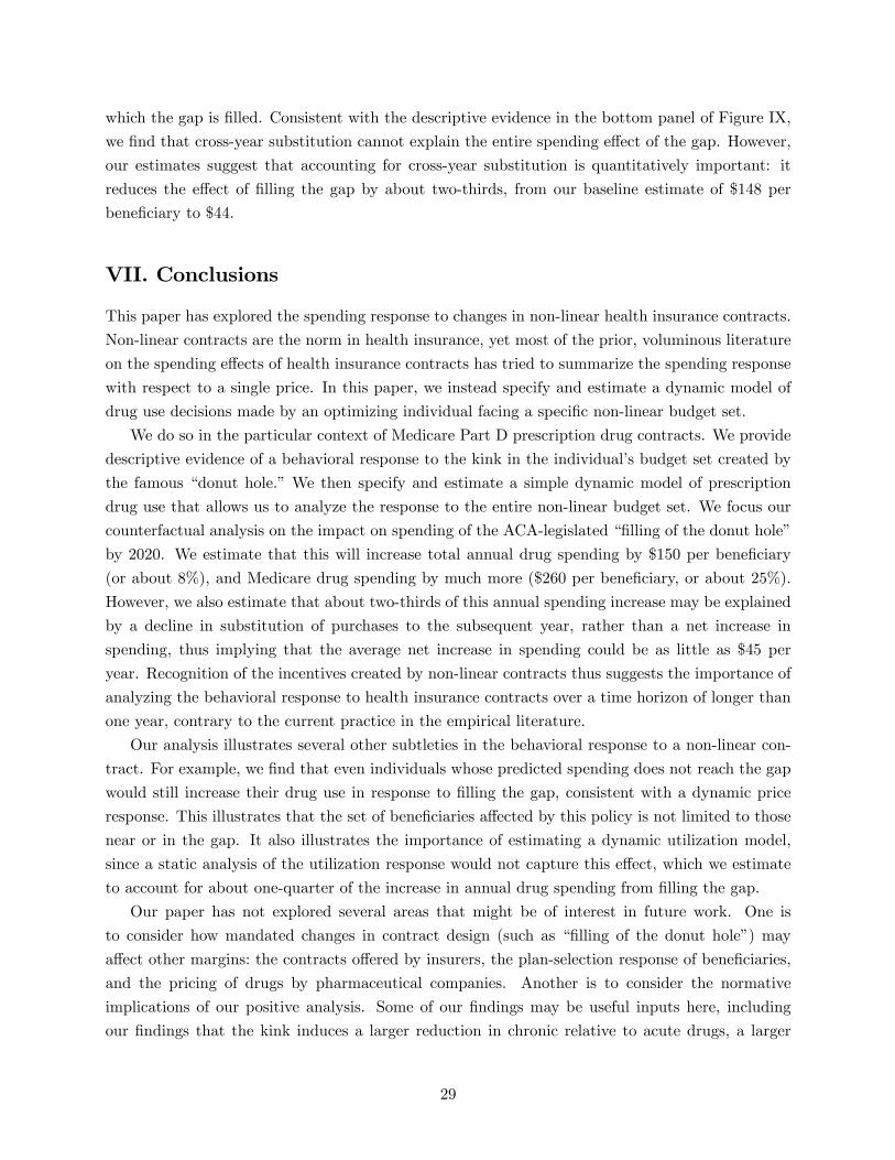
which the gap is �lled. Consistent with the descriptive evidence in the bottom panel of Figure IX,

we �nd that cross-year substitution cannot explain the entire spending e¤ect of the gap. However,

our estimates suggest that accounting for cross-year substitution is quantitatively important: it

reduces the e¤ect of �lling the gap by about two-thirds, from our baseline estimate of $148 per

bene�ciary to $44.

VII. Conclusions

This paper has explored the spending response to changes in non-linear health insurance contracts.

Non-linear contracts are the norm in health insurance, yet most of the prior, voluminous literature

on the spending e¤ects of health insurance contracts has tried to summarize the spending response

with respect to a single price. In this paper, we instead specify and estimate a dynamic model of

drug use decisions made by an optimizing individual facing a speci�c non-linear budget set.

We do so in the particular context of Medicare Part D prescription drug contracts. We provide

descriptive evidence of a behavioral response to the kink in the individual�s budget set created by

the famous �donut hole.�We then specify and estimate a simple dynamic model of prescription

drug use that allows us to analyze the response to the entire non-linear budget set. We focus our

counterfactual analysis on the impact on spending of the ACA-legislated ��lling of the donut hole�

by 2020. We estimate that this will increase total annual drug spending by $150 per bene�ciary

(or about 8%), and Medicare drug spending by much more ($260 per bene�ciary, or about 25%).

However, we also estimate that about two-thirds of this annual spending increase may be explained

by a decline in substitution of purchases to the subsequent year, rather than a net increase in

spending, thus implying that the average net increase in spending could be as little as $45 per

year. Recognition of the incentives created by non-linear contracts thus suggests the importance of

analyzing the behavioral response to health insurance contracts over a time horizon of longer than

one year, contrary to the current practice in the empirical literature.

Our analysis illustrates several other subtleties in the behavioral response to a non-linear con-

tract. For example, we �nd that even individuals whose predicted spending does not reach the gap

would still increase their drug use in response to �lling the gap, consistent with a dynamic price

response. This illustrates that the set of bene�ciaries a¤ected by this policy is not limited to those

near or in the gap. It also illustrates the importance of estimating a dynamic utilization model,

since a static analysis of the utilization response would not capture this e¤ect, which we estimate

to account for about one-quarter of the increase in annual drug spending from �lling the gap.

Our paper has not explored several areas that might be of interest in future work. One is

to consider how mandated changes in contract design (such as ��lling of the donut hole�) may

a¤ect other margins: the contracts o¤ered by insurers, the plan-selection response of bene�ciaries,

and the pricing of drugs by pharmaceutical companies. Another is to consider the normative

implications of our positive analysis. Some of our �ndings may be useful inputs here, including

our �ndings that the kink induces a larger reduction in chronic relative to acute drugs, a larger

29

reduction in drug use by healthier individuals, and that some (but not all) of the reduction in drug

use at the kink represents purchases postponed to the following year rather than foregone entirely.

Additional evidence on whether there are spillover e¤ects from prescription drug cost-sharing onto

non-drug healthcare spending (such as doctor visits and hospitalization) and to health might also

be informative on the normative dimension. More formal welfare analysis would also need to take

into account the optimality of drug consumption in the absence of insurance. For example, since

the policy of granting monopolies through the patent system produces drug prices above social

marginal cost, an insurance-induced increase in drug expenditures need not be socially ine¢ cient

(Lakdawalla and Sood 2009). Likewise, concerns that incomplete information or potential failures

of rationality may lead individuals to under-consume drugs in the absence of insurance raises

the possibility that insurance-induced increases in drug consumption may be e¢ ciency enhancing

(Baicker, Mullainathan, and Schwartzstein 2012).

Stanford University and NBER

Massachusetts Institute of Technology and NBER

University of British Columbia

References

Abaluck, Jason, and Jonathan Gruber, �Choice Inconsistencies Among the Elderly: Evidence from

Plan Choice in the Medicare Part D Program,�American Economic Review, 101 (2011), 1180-1210.

Abaluck, Jason, Jonathan Gruber, and Ashley Swanson, Prescription Drug Use under Medicare

Part D: A Linear Model of Nonlinear Budget Sets, Unpublished Mimeo (http://www.kellogg.northwestern.edu/

~/media/Files/Departments/hema/Conferences/Abaluck_Gruber_Swanson2014.ashx, 2014).

Alpert, Abby, The Anticipatory E¤ects of Medicare Part D on Drug Utilization, Unpublished

Mimeo (http://faculty.sites.uci.edu/aealpert/�les/2014/08/alpert_draft_aug2014.pdf, 2014).

Aron-Dine, Aviva, Liran Einav, and Amy Finkelstein, �The RAND Health Insurance Experi-

ment, Three Decades Later,�Journal of Economic Perspectives, 27 (2013), 197-222.

Aron-Dine, Aviva, Liran Einav, Amy Finkelstein, and Mark Cullen, �Moral Hazard in Health

Insurance: Do Dynamic Incentives Matter?�Review of Economics and Statistics, forthcoming, 2015.

Baicker, Katherine, Sendhil Mullainathan, and Joshua Schwartzstein, �Behavioral Hazard in

Health Insurance,�NBER Working Paper No. 18468, 2012.

Bajari, Patrick, Han Hong, Minjung Park, and Robert Town, �Regression Discontinuity Designs

with an Endogenous Forcing Variable and an Application to Contracting in Health Care,�NBER

Working Paper No. 17643, 2011.

Cabral, Marika, Claim Timing and Ex Post Adverse Selection, Unpublished Mimeo (http://www.

marikacabral.com/Cabral_ExPostAdverseSelection.pdf, 2013).

Chetty, Raj, �Bounds on Elasticities with Optimization Frictions: A Synthesis of Micro and

Macro Evidence on Labor Supply,�Econometrica, 80 (2012), 969-1018.

30

Chetty, Raj, John N. Friedman, Tore Olsen, and Luigi Pistaferri, �Adjustment Costs, Firm

Responses, and Micro vs. Macro Labor Supply Elasticities: Evidence from Danish Tax Records,�

Quarterly Journal of Economics, 126 (2011), 749-804.

Chetty, Raj, John N. Friedman, and Emmanuel Saez, �Using Di¤erences in Knowledge Across

Neighborhoods to Uncover the Impacts of the EITC on Earnings,�American Economic Review,

103 (2013), 2683-2721.

Dalton, Christina, �Estimating Demand Elasticities using Nonlinear Pricing,� International

Journal of Industrial Organization, 37 (2014), 178-191.

Dalton, Christina, Gautam Gowrisankaran, and Robert Town, Myopic and Complex Dynamic

Incentives: Evidence fromMedicare Part D, Unpublished Mimeo (http://www.utsc.utoronto.ca/~jcampbell/

PartD_hyperbolic.pdf, 2014).

Duggan, Mark, Patrick Healy, and Fiona Scott Morton, �Providing Prescription Drug Coverage

to the Elderly: America�s Experiment with Medicare Part D,� Journal of Economic Perspectives,

22 (2008), 69-92.

Duggan, Mark and Fiona Scott Morton, �The E¤ect of Medicare Part D on Pharmaceutical

Prices and Utilization,�American Economic Review, 100 (2010), 590-607.

Epstein, Larry G., and Stanley E. Zin, �Substitution, Risk Aversion, and The Temporal Be-

havior of Consumption and Asset Returns: A Theoretical Framework,�Econometrica, 57 (1989),

937-969.

Gentzkow, Matthew, and Jesse M. Shapiro, �Measuring the Sensitivity of Parameter Estimates

to Sample Statistics,�NBER Working Paper No. 20673, 2014.

Handel, Benjamin R., �Adverse Selection and Inertia in Health Insurance Markets: When

Nudging Hurts,�American Economic Review, 103 (2013), 2643-2682.

Hansen, Nikolaus, �The CMA Evolution Strategy: A Comparing Review,�Studies in Fuzziness

and Soft Computing, 192 (2006), 75-102.

Hansen, Nikolaus, and Stefan Kern, �Evaluating the CMA Evolution Strategy on Multimodal

Test Functions,�Lecture Notes in Computer Science, 3242 (2004), 282-291.

Hansen, Nikolaus, Anne Auger, Raymond Ros, Ste¤en Finck, and Petr Posik, �Comparing

Results of 31 Algorithms from The Black-Box Optimization Benchmarking BBOB-2009,� in Pro-

ceedings of The 12th Annual Conference Companion on Genetic and Evolutionary Computation,

1689-1696 (New York, NY: ACM, 2010).

Healthcare E¤ectiveness Data and Information Set (HEDIS), (Washington, DC: National Com-

mittee for Quality Assurance) (http://www.ncqa.org/tabid/59/default.aspx, 2010).

Heiss, Florian, Daniel McFadden, and Joachim Winter, �Mind the Gap! Consumer Perceptions

and Choices of Medicare Part D Prescription Drug Plans,�in Research Findings in the Economics

of Aging, David Wise, ed. (Chicago, IL: University of Chicago Press, 2010).

Heiss, Florian, Adam Leive, Daniel McFadden, and JoachimWinter, �Plan Selection in Medicare

Part D: Evidence from Administrative Data,�Journal of Health Economics, 32 (2013), 1325-1344.

Hu, Yingyao, and Matthew Shum, �Nonparametric Identi�cation of Dynamic Models with

Unobserved State Variables,�Journal of Econometrics, 171 (2012), 32-44.

31

Ito, Koichiro, �Do Consumers Respond to Marginal or Average Price? Evidence from Nonlinear

Electricity Pricing,�American Economic Review, 104 (2014), 537-563.

Joyce, Geo¤rey, Julie Zissimopoulos, and Dana Goldman, �Digesting the Doughnut Hole,�

Journal of Health Economics, 32 (2013), 1345-1355.

Kaiser Family Foundation, Medicare at a Glance (http://k¤.org/medicare/fact-sheet/medicare-

at-a-glance-fact-sheet, 2014).

Ketcham, Jonathan, Claudio Lucarelli, Eugenio Miravete, and M. Christopher Roebuck, �Sink-

ing, Swimming, or Learning to Swim in Medicare Part D,�American Economic Review, 102 (2012),

2639-2673.

Kleven, Henrik, and Mazhar Waseem, �Using Notches to Uncover Optimization Frictions and

Structural Elasticities: Theory and Evidence from Pakistan,�Quarterly Journal of Economics, 128

(2013), 669-723.

Kling, Je¤rey, Sendhil Mullainathan, Eldar Sha�r, Lee Vermeulen, and Marian Wrobel, �Com-

parison Friction: Experimental Evidence from Medicare Drug Plans,�Quarterly Journal of Eco-

nomics, 127 (2012), 199-235.

Kowalski, Amanda, �Estimating the Tradeo¤ Between Risk Protection and Moral Hazard with

a Nonlinear Budget Set Model of Health Insurance,�NBER Working Paper No. 18108, 2012.

Kreps, David M., and Evan L. Porteus, �Temporal Resolution of Uncertainty and Dynamic

Choice Theory,�Econometrica, 46 (1978), 185-200.

Lakdawalla, Darius, and Neeraj Sood, �Innovation and the Welfare E¤ects of Public Drug

Insurance,�Journal of Public Economics, 93 (2009), 541-548.

Manoli, Dayand, and Andrea Weber, �Nonparametric Evidence on the E¤ects of Financial

Incentives on Retirement Decisions,�NBER Working Paper No. 17320, 2011.

Polyakova, Maria, Regulation of Insurance with Adverse Selection and Switching Costs: Evi-

dence from Medicare Part D, Unpublished Mimeo (http://web.stanford.edu/~mpolyak/Polyakova_

PartD_inertia.pdf, 2014).

Rios, Luis Miguel, and Nikolaos V. Sahinidis, �Derivative-Free Optimization: A Review of

Algorithms and Comparison of Software Implementations,� Journal of Global Optimization 56

(2013), 1247-1293.

Saez, Emmanuel, �Do Taxpayers Bunch at Kink Points?,�American Economic Journal: Eco-

nomic Policy, 2 (2010), 180-212.

Vera-Hernandez, Marcos, �Structural Estimation of a Principal-Agent Model: Moral Hazard in

Medical Insurance,�RAND Journal of Economics, 34 (2003), 670-693.

Yin, Wesley, Anirban Basu, James Zhang, Atonu Rabbani, David Meltzer, and Caleb Alexander,

�The E¤ect of the Medicare Part D Prescription Bene�t on Drug Utilization and Expenditures,�

Annals of Internal Medicine, 148 (2008), 169-177.

Zhang, Yuting, Katherine Baicker, and Joseph P. Newhouse, �Geographic Variation in the

Quality of Prescribing,�New England Journal of Medicine 363 (2010), 1985-1988.

32

Figure I: The Standard Medicare Part D Bene�t Design in 2008

Figure shows the standard bene�t design in 2008. �Pre-Kink coverage�refers to coverage prior to the Initial Coverage

Limit (ICL) which is where there is a kink in the budget set and the gap, or donut hole, begins. As described in

the text, the actual level at which the catastrophic coverage kicks in is de�ned in terms of out-of-pocket spending (of

$4,050), which we convert to the total expenditure amount provided in the �gure. Once catastrophic coverage kicks

in, the actual standard coverage speci�es a set of co-pays (dollar amounts) for particular types of drugs, while in the

�gure we use instead a 7% co-insurance rate, which is the empirical average of these co-pays in our data.

33

Figure II: The Distribution of Annual Drug Expenditure for Medicare Part D Enrolleesin 2008

Figure displays the distribution of total annual prescription drug spending in 2008 for our baseline sample. Each bar

represents the set of people that spent up to $100 above the value that is on the x-axis, so that the �rst bar represents

individuals who spent less than $100 during the year, the second bar represents $100-200 spending, and so on. For

visual clarity, we omit from the graph the 3% of the sample whose spending exceeds $6,500. The kink location (in

2008) is at $2,510. N =1,251,984.

34

Figure III: The Distribution of Annual Drug Expenditure around The Kink, for each YearSeparately

Figure displays the distribution of total annual prescription drug spending, separately by year, for individuals in our

baseline sample whose annual spending in a given year was between $1,500 and $3,500 (N=1,332,748 overall; by year

it is 447,012 (2007), 443,323 (2008), and 442,413 (2009)). Each point in the graph represents the set of people that

spent up to $20 above the value that is on the x-axis, so that the �rst point represents individuals who spent between

$1,500 and $1,520, the second bar represents $1,520-1,540 spending, and so on. We normalize the frequencies so that

they add up to one for each series (year) shown.

35

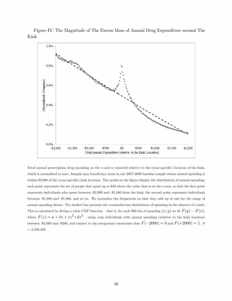
Figure IV: The Magnitude of The Excess Mass of Annual Drug Expenditure around TheKink

Total annual prescription drug spending on the x-axis is reported relative to the (year-speci�c) location of the kink,

which is normalized to zero. Sample uses bene�ciary-years in our 2007-2009 baseline sample whose annual spending is

within $2,000 of the (year-speci�c) kink location. The points in the �gure display the distribution of annual spending;

each point represents the set of people that spent up to $20 above the value that is on the x-axis, so that the �rst point

represents individuals who spent between -$2,000 and -$1,980 from the kink, the second point represents individuals

between -$1,980 and -$1,960, and so on. We normalize the frequencies so that they add up to one for the range of

annual spending shown. The dashed line presents the counterfactual distribution of spending in the absence of a kink.

This is calculated by �tting a cubic CDF function �that is, for each $20 bin of spending (x; y) we �t F (y)� F (x),where F (z) = a+ bz + cz2+dz3 � using only individuals with annual spending (relative to the kink location)

between -$2,000 and -$200, and subject to the integration constraints that F (�2000) = 0 and F (+2000) = 1. N= 2,589,458.

36

Figure V: The Decline in The Propensity to Claim Toward The End of The CalendarYear

Each panel of the �gure shows the fraction of individuals who have at least one drug purchase during the

corresponding month (which appears in the panel title) as a function of their total annual spending. The

x-axis reports total annual spending relative to the (year-speci�c) kink location, which is normalized to

zero. Each point in the graph represents individuals who spend within $20 above the value on the x-axis.

The dashed line in each panel is generated by regressing the logarithm of the share of individuals with no

purchase (in the panel-speci�c month) in each $20 spending bin, using only individuals with annual spending

(relative to the kink location) between -$2,000 and -$500, on the mid-point of the spending amount in the

bin, weighting each bin by the number of bene�ciaries in that bin. Data are our baseline sample in 2007-2009

whose annual spending is within $2,000 of the kink location (N=2,589,458).

37

Figure VI: Actual and Predicted Distributions of Annual Drug Expenditure

Figure shows the distribution of observed and predicted total annual drug spending. The top panel shows the results

for the whole distribution, where each bar represents a $100 spending bin above the value on the x-axis (except for

the last bar, which includes all spending above $5,900). The bottom panel �zooms in�on spending within $1,000 of

the (year-speci�c) kink (which is normalized to 0) and shows observed and predicted spending in $20 bins, where each

point represents individuals who spend within $20 above the value on the x-axis. Frequencies in the bottom panel are

normalized to sum to 1 across the displayed range. We note that the �gure is based on the estimation sample rather

than the baseline sample (see footnote 23), so the summary statistics do not perfectly match those presented

in Table I.

38

Figure VII: Actual and Predicted Propensity to Claim for Each Calendar Month

Figure shows the claim timing pattern of the observed and predicted spending. The x-axis represents calendar

�months�(where a month is a group of four weeks, so we have 13 such �months�in a coverage year), and the y-axis

reports the observed and predicted share of individuals who have at least one claim during that �month.�The gray

lines show this pattern for individuals who (by the end of the year) are well below the kink: their overall spending is

between 800 and 500 dollars below the (year-speci�c) kink. These individuals tend to increase their monthly spending

over the calendar year as a greater fraction of them hits the deductible and enter the pre-kink coverage arm. The

black lines show this pattern for individual who end up around the kink (within 150 dollars of it, on both sides).

These individuals decrease their propensity to claim toward the end of the year, as shown (in more details) in Figure

V.

39

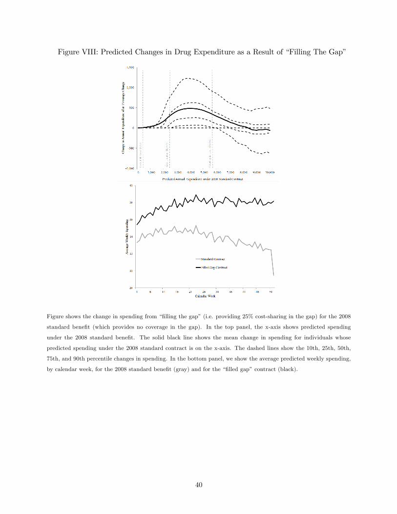
Figure VIII: Predicted Changes in Drug Expenditure as a Result of �Filling The Gap�

Figure shows the change in spending from ��lling the gap�(i.e. providing 25% cost-sharing in the gap) for the 2008

standard bene�t (which provides no coverage in the gap). In the top panel, the x-axis shows predicted spending

under the 2008 standard bene�t. The solid black line shows the mean change in spending for individuals whose

predicted spending under the 2008 standard contract is on the x-axis. The dashed lines show the 10th, 25th, 50th,

75th, and 90th percentile changes in spending. In the bottom panel, we show the average predicted weekly spending,

by calendar week, for the 2008 standard bene�t (gray) and for the ��lled gap�contract (black).

40

Figure IX: Descriptive Evidence of Substitution of Claims from The End of The CalendarYear to The Beginning of The Next Year

The top panel shows the individual�s relative January spending in year y + 1 as a function of her total annual

spending (relative to the kink location, which is normalized to 0) in the prior year (year y). �Relative� January

spending in year y + 1 is de�ned as the ratio of January spending in year y + 1 to average monthly spending in

March through June (of year y + 1). Each bar on the graph represents individuals within $50 above the value on the

x-axis. The y-axis reports the average, for each year y spending bin, of the �relative January spending�measure. The

dashed, horizontal �counterfactual�relative January spending is calculated as the average relative January spending

for people -500 to -2000 below the kink in year y: This analysis is limited to individuals in our baseline sample in

2007 and 2008 whom we observe in the subsequent year; we exclude individuals in our baseline sample in 2009 since

we do not observe their year y + 1 spending. N=1,534,952.

The bottom panel shows the bunching analysis (from Figure IV), but now as a function of �adjusted�annual spending.

�Adjusted�annual spending is computed by taking total annual spending (in year y) and, for each $50 bin of annual

spending in year y, adding the average dollar di¤erence between January spending in year y + 1 and the average

monthly spending in March to June of year y + 1. �Adjusted� annual spending is reported relative to the kink

location in year y (which is normalized to 0). The sample shown is once again limited to our baseline sample in 2007

and 2008 whom we observe in the subsequent year (N=1,534,952).

41

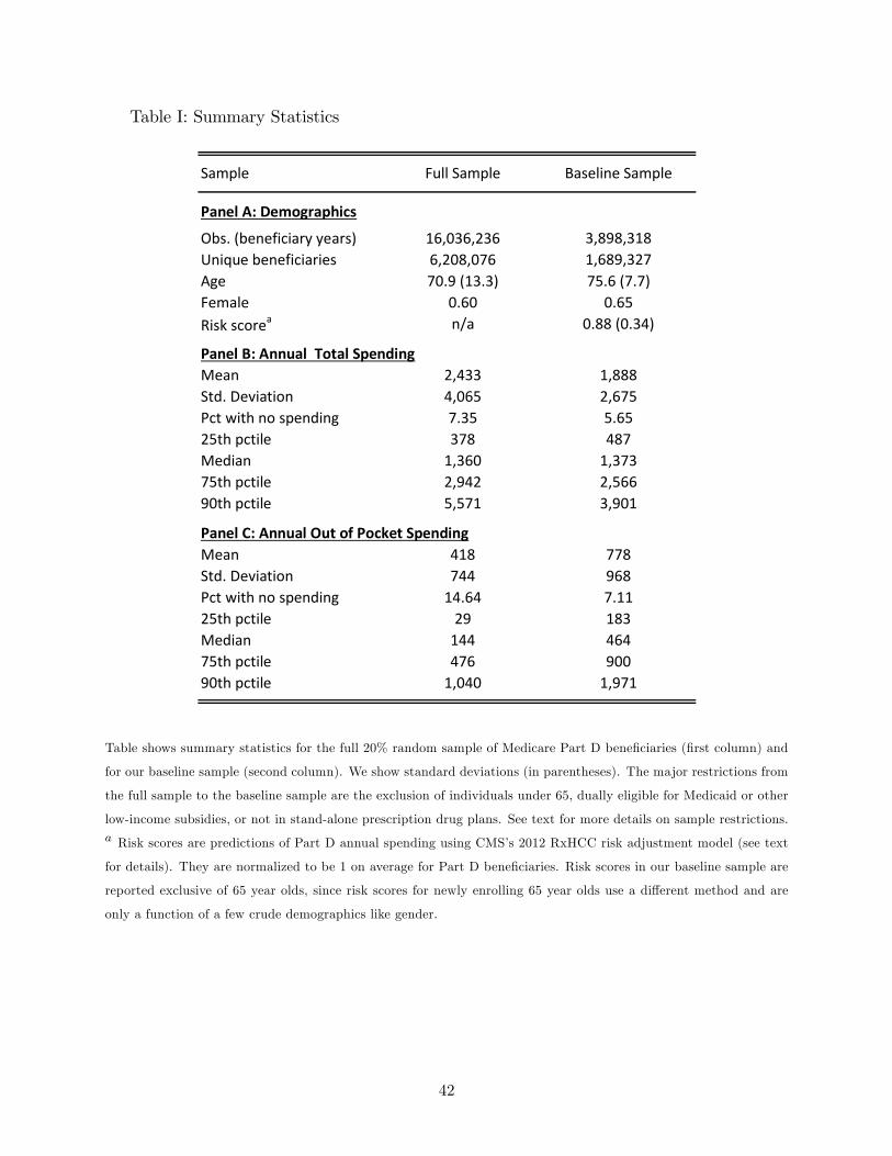
Table I: Summary Statistics

Sample Full Sample Baseline Sample

Panel A: Demographics

Obs. (beneficiary years) 16,036,236 3,898,318Unique beneficiaries 6,208,076 1,689,327Age 70.9 (13.3) 75.6 (7.7)Female 0.60 0.65Risk scorea n/a 0.88 (0.34)

Panel B: Annual  Total SpendingMean 2,433 1,888Std. Deviation 4,065 2,675Pct with no spending 7.35 5.6525th pctile 378 487Median 1,360 1,37375th pctile 2,942 2,56690th pctile 5,571 3,901

Panel C: Annual Out of Pocket SpendingMean 418 778Std. Deviation 744 968Pct with no spending 14.64 7.1125th pctile 29 183Median 144 46475th pctile 476 90090th pctile 1,040 1,971

Table shows summary statistics for the full 20% random sample of Medicare Part D bene�ciaries (�rst column) and

for our baseline sample (second column). We show standard deviations (in parentheses). The major restrictions from

the full sample to the baseline sample are the exclusion of individuals under 65, dually eligible for Medicaid or other

low-income subsidies, or not in stand-alone prescription drug plans. See text for more details on sample restrictions.a Risk scores are predictions of Part D annual spending using CMS�s 2012 RxHCC risk adjustment model (see text

for details). They are normalized to be 1 on average for Part D bene�ciaries. Risk scores in our baseline sample are

reported exclusive of 65 year olds, since risk scores for newly enrolling 65 year olds use a di¤erent method and are

only a function of a few crude demographics like gender.

42

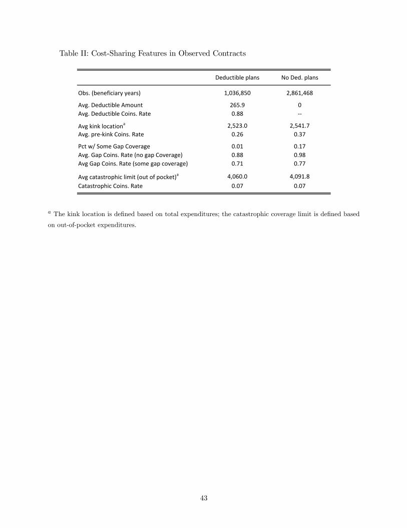
Table II: Cost-Sharing Features in Observed Contracts

Deductible plans No Ded. plans

Obs. (beneficiary years) 1,036,850 2,861,468

Avg. Deductible Amount 265.9 0Avg. Deductible Coins. Rate 0.88 ­­

Avg kink locationa 2,523.0 2,541.7Avg. pre­kink Coins. Rate 0.26 0.37

Pct w/ Some Gap Coverage 0.01 0.17Avg. Gap Coins. Rate (no gap Coverage) 0.88 0.98Avg Gap Coins. Rate (some gap coverage) 0.71 0.77

Avg catastrophic limit (out of pocket)a 4,060.0 4,091.8Catastrophic Coins. Rate 0.07 0.07

a The kink location is de�ned based on total expenditures; the catastrophic coverage limit is de�ned based

on out-of-pocket expenditures.

43

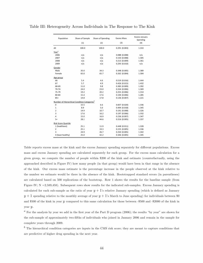
Table III: Heterogeneity Across Individuals in The Response to The Kink

Population Share of Sample Share of SpendingExcess January

Spending(1) (2) (4)

All 100.0 100.0 0.291 (0.003) 1.333

Yeara

   2006 n/a n/a 0.088 (0.008) n/a   2007 n/a n/a 0.150 (0.008) 1.305   2008 n/a n/a 0.213 (0.009) 1.361   2009 n/a n/a 0.293 (0.010) n/a

Gender   Male 35.0 34.3 0.348 (0.005) 1.389   Female 65.0 65.7 0.262 (0.004) 1.304

Age group   66 5.4 4.6 0.519 (0.016) 1.444   67 5.7 4.9 0.426 (0.015) 1.432   68­69 11.0 9.8 0.383 (0.009) 1.392   70­74 24.0 23.0 0.334 (0.006) 1.369   75­79 19.2 20.2 0.255 (0.006) 1.314   80­84 15.4 17.6 0.194 (0.006) 1.285   85+ 14.8 17.8 0.136 (0.007) 1.221

Number of Hierarchical Condition Categoriesb

   0 15.5 6.6 0.837 (0.020) 1.336   1 8.9 5.0 0.494 (0.018) 1.345   2 14.9 10.7 0.191 (0.008) 1.326   3 17.6 16.2 0.197 (0.006) 1.332   4 15.0 16.9 0.236 (0.007) 1.347   5+ 28.1 44.6 0.316 (0.005) 1.337

Risk Score Quartile   1 (healthiest) 25.1 11.9 0.448 (0.011) 1.328   2 25.1 19.3 0.155 (0.005) 1.336   3 24.9 26.7 0.250 (0.005) 1.342   4 (least healthy) 25.0 42.2 0.346 (0.005) 1.345

Excess Mass

(3)

Table reports excess mass at the kink and the excess January spending separately for di¤erent populations. Excess

mass and excess January spending are calculated separately for each group. For the excess mass calculation for a

given group, we compute the number of people within $200 of the kink and estimate (counterfactually, using the

approached described in Figure IV) how many people (in that group) would have been in that range in the absence

of the kink. Our excess mass estimate is the percentage increase in the people observed at the kink relative to

the number we estimate would be there in the absence of the kink. Bootstrapped standard errors (in parentheses)

are calculated based on 500 replications of the bootstrap. Row 1 shows the results for the baseline sample (from

Figure IV; N =2,589,458). Subsequent rows show results for the indicated sub-samples. Excess January spending is

calculated for each sub-sample as the ratio of year y + 1�s relative January spending (which is de�ned as January

y + 1 spending relative to the monthly average of year y + 1�s March to June spending) for individuals between $0

and $500 of the kink in year y compared to this same calculation for those between -$500 and -$2000 of the kink in

year y:a For the analysis by year we add in the �rst year of the Part D program (2006); the results �by year�are shown for

the sub-sample of approximately two-�fths of individuals who joined in January 2006 and remain in the sample for

complete years through 2009.b The hierarchical condition categories are inputs in the CMS risk score; they are meant to capture conditions that

are predictive of higher drug spending in the next year.

44

Table IV: Heterogeneity across Types of Drugs in The Response to The Kink

Actual PredictedP(Dec. Purchase) P(Dec. Purchase)

(1) (2) (3) (4) (6)

All 100.0 100.0 0.846 0.923 0.083  (0.001) 1.333

Chronic 69.6 77.1 0.762 0.867 0.121  (0.001) 1.323Acute 30.4 22.9 0.532 0.590 0.099  (0.002) 1.335

Maintenance 85.1 90.1 0.807 0.899 0.103  (0.001) 1.350Non­Maintenance 14.9 9.9 0.303 0.330 0.080  (0.004) 1.151

Brand 33.4 74.8 0.624 0.780 0.199  (0.001) 1.362Generic 66.6 25.2 0.731 0.798 0.085  (0.001) 1.235

"Inappropriate" a 2.7 1.3 0.075 0.085 0.119  (0.009) 1.262

Excess Januaryspending

(5)

Percent ofpurchases

Percent ofspending ($)

Drug TypePercent decrease inpurchase probability

Table shows overall, and then separately by drug type, the change in the probability of a purchase in December

around the kink location. The analysis is done on the same sample analyzed in Figure V (N=2,589,458). The �actual�

probability of a December purchase (column (3)) is the probability someone whose annual spending is within $200

of the kink location �lls at least one prescription in December. The �predicted�probability of a December purchase

within $200 of the kink location (column (4)) is designed to re�ect what the probability of a December purchase

would have been in the absence of the kink. It is estimated (as in the dashed line in Figure V) by regressing the

logarithm of the share of individuals with no December purchase in each $20 spending bin (between -$2,000 and

-$500) on the mid-point of the spending amount in the bin, weighting each bin by the number of bene�ciaries in that

bin. When looking separately by drug type, the �actual� and �predicted�probabilities are calculated based on the

probability of a purchase for a speci�c drug type. Column (5) shows the percent decrease in purchase probability,

i.e. the predicted minus actual December purchase probability as a percent of the predicted. Bootstrapped standard

errors (in parentheses) are calculated by estimating the actual and predicted probability of a December purchase of

a given type based on 500 bootstrap replications. In column (6) we report excess January spending (in year y + 1)

for each drug type. Excess January spending is calculated for each sub-sample as the ratio of year y + 1�s relative

January spending (which is de�ned as January y + 1 spending relative to the monthly average of year y + 1�s March

to June spending) for individuals between $0 and $500 of the kink in year y compared to this same calculation for

those between -$500 and -$2000 of the kink in year y:a Following Zhang, Baicker, and Newhouse (2010), we proxy for inappropriate drug use using an indicator from

the Healthcare E¤ectiveness Data and Information Set (HEDIS) on whether the drug is considered high-risk for the

elderly (HEDIS 2010).

45

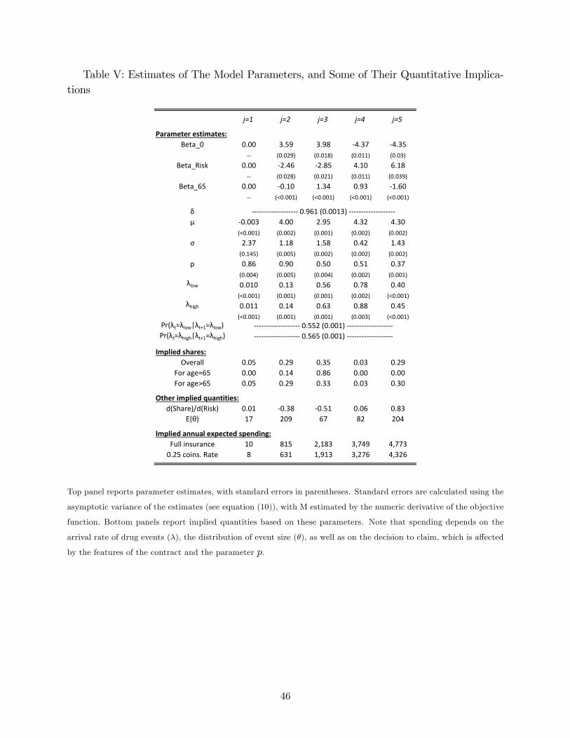
Table V: Estimates of The Model Parameters, and Some of Their Quantitative Implica-tions

j=1 j=2 j=3 j=4 j=5

Parameter estimates:Beta_0 0.00 3.59 3.98 ­4.37 ­4.35

­­ (0.029) (0.018) (0.011) (0.03)

Beta_Risk 0.00 ­2.46 ­2.85 4.10 6.18­­ (0.028) (0.021) (0.011) (0.039)

Beta_65 0.00 ­0.10 1.34 0.93 ­1.60­­ (<0.001) (<0.001) (<0.001) (<0.001)

δμ ­0.003 4.00 2.95 4.32 4.30

(<0.001) (0.002) (0.001) (0.002) (0.002)

σ 2.37 1.18 1.58 0.42 1.43(0.145) (0.005) (0.002) (0.002) (0.002)

p 0.86 0.90 0.50 0.51 0.37(0.004) (0.005) (0.004) (0.002) (0.001)

λlow 0.010 0.13 0.56 0.78 0.40(<0.001) (0.001) (0.001) (0.002) (<0.001)

λhigh 0.011 0.14 0.63 0.88 0.45(<0.001) (0.001) (0.001) (0.003) (<0.001)

Pr(λt=λlow|λt+1=λlow)Pr(λt=λhigh|λt+1=λhigh)

Implied shares:Overall 0.05 0.29 0.35 0.03 0.29

For age=65 0.00 0.14 0.86 0.00 0.00For age>65 0.05 0.29 0.33 0.03 0.30

Other implied quantities:d(Share)/d(Risk) 0.01 ­0.38 ­0.51 0.06 0.83

E(θ) 17 209 67 82 204

Implied annual expected spending:Full insurance 10 815 2,183 3,749 4,773

0.25 coins. Rate 8 631 1,913 3,276 4,326

­­­­­­­­­­­­­­­­­­­ 0.961 (0.0013) ­­­­­­­­­­­­­­­­­­­

­­­­­­­­­­­­­­­­­­­ 0.552 (0.001) ­­­­­­­­­­­­­­­­­­­­­­­­­­­­­­­­­­­­­­ 0.565 (0.001) ­­­­­­­­­­­­­­­­­­­

Top panel reports parameter estimates, with standard errors in parentheses. Standard errors are calculated using the

asymptotic variance of the estimates (see equation (10)), with M estimated by the numeric derivative of the objective

function. Bottom panels report implied quantities based on these parameters. Note that spending depends on the

arrival rate of drug events (�), the distribution of event size (�), as well as on the decision to claim, which is a¤ected

by the features of the contract and the parameter p.

46

Table VI: Estimates for The Average Change in Drug Expenditure as a Result of �FillingThe Gap�

Mean Std. Dev. 25th pctile Median 90th pctile Mean OOP Mean Insurer

Assign everyone to Standard 2008 contract:1 Baseline 1,760 1,924 402 1,413 3,632 809 951

2 "Filled" gapa 1,964 2,127 407 1,455 4,450 655 1,309

Assign everyone observed (chosen) contract:3 Baseline 1,768 1,909 499 1,342 3,675 796 973

4 "Filled" gapa 1,916 2,051 502 1,371 4,287 690 1,226

Assign everyone observed (chosen) contract, plus allow cross­year substitution:5 Baseline 1,770 1,912 501 1,337 3,749 807 963

6 "Filled" gapa 1,814 1,964 501 1,341 3,956 658 1,155

Table reports the predicted annual drug spending under various observed and counterfactual contracts. All columns

report total annual drug spending except the rightmost two which separately report out-of-pocket and insurer spend-

ing. Rows 1 and 2 report predicted spending under the standard contract in 2008, which was illustrated in Figure I,

and counterfactual changes to it. Rows 3 and 4 report predicted spending for the observed contracts in our sample,

and counterfactual changes to them. Rows 5 and 6 repeat the same exercise (as in rows 3 and 4), but use the extension

of the model that accounts of cross-year substitution. For all of the simulations, we assume individuals are in the

contract for a full 12 months. (Predicted mean spending for observed contracts - row 3 - is slightly higher than the

estimate reported in the top panel of Figure VI because of the assumption here that everyone is in the contract for

12 months).a �Filling the gap�means that, above the deductible, the plan now has a constant co-insurance rate, without a kink,

until out-of-pocket expenditure hits the catastrophic limit. For each plan, we use the observed (pre-kink) co-insurance

rate (which is 25% in the 2008 standard bene�t plan.). For the less than 1% of plans where our calculated pre-kink

co-insurance rate is higher than our calculated co-insurance rate in the gap, we do not adjust cost-sharing in the

counterfactual.

47

Table VII: Robustness of The Key Results to Various Modeling Assumptions

Baseline "Filled" Gap Change Baseline "Filled" Gap Change

1 Baseline model 1,768 1,916 8.4% 973 1,226 26.0%

Number of types:2 Three types 1,778 1,878 5.6% 986 1,208 22.5%3 Six types 1,760 1,937 10.1% 967 1,240 28.2%

Different sets of covariates:4 Remove all covariates 1,783 1,892 6.1% 976 1,209 23.9%5 Add "no gap" covariate 1,758 1,946 10.7% 968 1,246 28.7%

Concave (risk averse) utility function:6 CARA = exp(­6.5) 1,737 1,873 7.8% 945 1,193 26.2%7 CARA = exp(­9.5) 1,738 1,862 7.1% 940 1,183 25.9%

Distribution of ω:8 ω correlated with θ 1,781 1,918 7.7% 983 1,230 25.1%

Total Spending Insurer Spending

Table shows how the predictions of the model are a¤ected by di¤erent speci�cations of the economic or econometric

model. The �rst row presents the results from the baseline model (as reported in rows 3 and 4 of Table V). Row 2 and

3 report results in which we explore the sensitivity of the results to the number of discrete types (M): the baseline

model assumes M = 5, while row 2 assumes M = 3, and row 3 assumes M = 6. Row 4 reports results in which

we do not use any covariates zi to estimate the propensity of each individual to be of each type, while row 5 uses the

baseline covariates (a risk score, and an indicator for a 65 year old) and also adds an additional covariate, an indicator

for a bene�ciary who selected a plan with no gap coverage. Rows 6 and 7 report results that are based on estimating

a recursive utility model that allows for risk aversion as described in the main text (relative to the risk neutrality

assumption of the baseline model). The two values of the (absolute) risk aversion parameter are imposed, such that

they span the range of risk aversion estimates reported in Handel (2013). Finally, row 8 reports an extension of the

model that allows the moral hazard parameter p to vary with �; as described in the main text.

48