THE RELATIONSHIP BETWEEN LOAN DEFAULT AND THE FINAN CIAL

PERFORMANCE OF SACCOS IN KENYA

NANCY JEMOEK KEITANY

REG NO.D61/66866/2011

SUPERVISOR: DR.J ADUDA

A RESEARCH PROJECT PRESENTED IN PARTIAL FULFILMENT OF THE

REQUIREMENTS OF THE AWARD OF THE DEGREE OF MASTER O F

BUSINESS ADMINISTRATION, UNIVERSITY OF NAIROBI.

OCTOBER 2013

ii

DECLARATION

This research project is my original work and has never been presented in any other

University or college for award of degree, diploma or certificate.

Sign……………………………… Date……………………………

NANCY JEMOEK KEITANY

D61/66866/2011

This research project has been submitted for examination with my approval as University

supervisor

Sign……………………………… Date……………………………

Dr .Josiah Aduda

Supervisor,

Department of Finance and Accounting,

School of Business,

University of Nairobi.

iii

ACKNOWLEDGEMENT I am greatly indebted to many people who enabled me complete my study.

I would like to single out my supervisor Dr Aduda who dedicated a lot of time and effort

to my work. This study would not have been successful without his comments, advice,

suggestions and encouragement.

I would like to thank Sacco Societies Regulatory Authority for unconditionally availing

me the information required.

I would also pass my appreciation to the University for the Opportunity granted to

acquire knowledge required to accomplish this project.

I would also thank my employer for the time and resources used to accomplish this

undertaking.

iv

DEDICATION

I dedicate this work to my husband Daniel Kipkoech and my children Ruth, Paul and

Walter because of their moral support, encouragement, understanding and sacrifice.

v

ABSTRACT

Loan default is the failure to pay back a loan which may occur if the debtor is either

unwilling or unable to pay its debt. A defaulted loan is a cost to SACCOs in terms of

forgone or delayed interest, high recovery cost and finance cost associated with external

borrowing. The study sought to review the relationship between loan default and the

financial performance of Savings and Credit Cooperative Societies (SACCOs) in Kenya.

The research design used in this study was descriptive design. The design was

appropriate because the study involved in depth information on the relationship between

loan default and the financial performance of SACCOs. Data was collected from the

census of 45 SACCCOs in Nairobi County using secondary data from SASRA, which is

the regulatory body thus the study concentrated on 20 SACCOs. The data was reviewed,

and analyzed using (SPSS version 18) both descriptive and inferential statistics.

The study findings indicated that there is strong negative relationship between the loan

default and the profitability of these SACCOS. The tests showed that the overall

regression model is a good fit for the data as the independent variables statistically and

significantly predict the dependent variable. The regression model is a good fit of the

data. Personality types are predisposed to loan default why credit markets may fail. The

study recommends that SACCO should; continuously review credit policies, establish

irrecoverable loan provision policies, and character of loan applicants.

.

vi

TABLE OF CONTENTS

DECLARATION ............................................................................................................................ ii

ACKNOWLEDGEMENT ............................................................................................................. iii

DEDICATION............................................................................................................................... iv

ABSTRACT.................................................................................................................................... v

TABLE OF CONTENTS............................................................................................................... vi

LIST OF TABLES & FIGURES ................................................................................................. viii

ACRONYMS................................................................................................................................. ix

ACRONYMS................................................................................................................................. ix

CHAPTER ONE ............................................................................................................................. 1

INTRODUCTION .......................................................................................................................... 1

1.1 Background of the study ....................................................................................................... 1

1.1.1 Loan Defaul ................................................................................................................... 2

1.1.2 Financial Performance ................................................................................................... 3

1.1.3 Relationship of loan default on financial performance.................................................. 4

1.1.4 Sacco’s in Kenya............................................................................................................ 5

1.2 Research Problem ................................................................................................................. 6

1.4 Research Objective ............................................................................................................... 8

1.5 Significance of the study....................................................................................................... 8

CHAPTER TWO ............................................................................................................................ 9

LITERATURE REVIEW ............................................................................................................... 9

2.1 Introduction........................................................................................................................... 9

2.2 Theoretical Review ............................................................................................................... 9

2.2.1Theory of Group Formation.......................................................................................... 10

2.2.2. Theory of Credit Default............................................................................................. 10

2.2.3 Theory of micro-loan borrowing rates & default......................................................... 11

2.2.4 Default Risk Models .................................................................................................... 12

2.3 Financial Performance Measures........................................................................................ 15

2.3.1 Liquitity........................................................................................................................ 15

2.3.2. Earnings ...................................................................................................................... 15

2.3.4 Turnover....................................................................................................................... 16

vii

2.4 Empirical Studies................................................................................................................ 16

2.5 Conclusion from Literature Review.................................................................................... 21

CHAPTER THREE ...................................................................................................................... 23

RESEARCH METHODOLOGY.................................................................................................. 23

3.1 Introduction......................................................................................................................... 23

3.2 Research design .................................................................................................................. 23

3.3 Target Population................................................................................................................ 23

3.4 Sampling design................................................................................................................. 24

3.5 Data collection procedures.................................................................................................. 24

3.6 Data analysis and Presentation............................................................................................ 24

CHAPTER FOUR......................................................................................................................... 24

DATA ANALYSIS, RESULTS AND DISCUSSION .................................................................26

4.1. Introduction........................................................................................................................ 26

4.2 The relationship between loan default and turnover........................................................... 26

4.3: Relationship between loan default and Assets................................................................... 29

4.4 Relationship between loan default and equity .................................................................... 31

4.5 Summary of variables ......................................................................................................... 33

4.6 Analysis of no variance....................................................................................................... 34

4.7 Summary and Interpretation of the Findings ...................................................................... 37

CHAPTER FIVE .......................................................................................................................... 41

SUMMARY, CONCLUSION AND RECOMMENDATIONS................................................... 41

5.1 Summary Of Findings........................................................................................................ 41

5. 2.Conclusions........................................................................................................................ 42

5.3 Policy Recommendations.................................................................................................... 43

5.4. Limitations of the study ..................................................................................................... 44

5.5. Recommendations for further research.............................................................................. 45

REFERENCES ............................................................................................................................. 47

APPENDICES .............................................................................................................................. 51

APPENDIX I: List of Licenced SACCOs by Sacco Society Regulatory Authority as at 31st December 2012 .................................................................................................................. 51

APPENDIX II: DATA COLLECTION FORM ....................................................................... 53

viii

LIST OF TABLES & FIGURES

Table.1 correlations between loan default and turnover............................................................... 26

Fig.1: scatter diagram loan default versus turnover...................................................................... 27

Table.2: model summary of the correlations between loan default and the turnover................... 28

Table.3: correlations between loan default and Assets................................................................. 29

Fig.2: scatter diagram loan default versus assets .......................................................................... 30

Table.4: correlations between loan default and equity ................................................................. 31

Fig.3: scatter diagram loan default versus assets .......................................................................... 32

Table.5: Summary of correlations of variables............................................................................. 33

Table.6: Analysis of no variance .................................................................................................. 34

Table.7: Model summary. ............................................................................................................. 35

Table.8: Model coefficients .......................................................................................................... 36

ix

ACRONYMS

SACCO-Savings and credit co-operatives

RBA- Retirement Benefit Authority

KCC-Kenya creameries co-operatives

KFA-Kenya farmers union

KPCU-Kenya planters’ co-operative Union

ROE-Return on equity

ROSCAS-Rotating Savings and Credit Associations

PD-Probability of default

LGD-Loss given default

RR-Recovery rate

EAD-Exposure at default

ICA-International Co-operative Alliance

ROA- Return on Assets

OPM-Operating Profit Margin

ATR-Asset Turnover Ratio

SPSS-Statistical Package for Social Sciences

AMT-African Microfinance Transparency

AMFIU- Association of Microfinance Institutions of Uganda

1

CHAPTER ONE

INTRODUCTION

1.1 Background of the study

In accordance to study of Nicholas (2010) default occurs when a debtor has not met his

or her legal obligations according to the debt contract, for example has not made a

scheduled payment, or has violated a loan covenant (condition) of the debt contract. A

default is the failure to pay back a loan. Default may occur if the debtor is either

unwilling or unable to pay his or her debt. This can occur with all debt obligations

including bonds, mortgages, loans, and notes. In corporate finance, upon an uncured

default, the holders of the debt will usually initiate proceedings (file a petition of

involuntary bankruptcy) to foreclose on any collateral securing the debt. Even if the debt

is not secured by collateral, debt holders may still sue for bankruptcy, to ensure that the

corporation's assets are used to repay the debt.

According to David and Lando (2004) default can be of several types: debt services

default, technical default, sovereign default, orderly default, strategic default, sovereign

strategic default and consumer default. Debt service default occurs when the borrower

has not made a scheduled payment of interest or principal. Technical default occurs when

an affirmative or a negative covenant is violated. With most debt (including corporate

debt, mortgages and bank loans) a covenant is included in the debt contract which states

that the total amount owed becomes immediately payable on the first instance of a default

of payment. Generally, if the debtor defaults on any debt to the lender, a cross

default covenant in the debt contract states that that particular debt is also in default.

2

According to the study of Uboun (1998) SACCOs societies grant loans on the basis of

member’s savings. The loan may be more or less than the savings of the borrower. Loans

less than the member savings are secure and the repayment is assured .Loans in excess of

the members savings must be guaranteed by other members. Loans that are not recovered

are considered to be delinquent and hence defaulted. Steams (1991) study found out that

the manner in which borrowers are selected and the amount of loan given to each

successful borrower determines the magnitude of loan delinquency. Borrowers who are

given loans they can repay without hardships hardly default. All shares owed by

defaulters and any dividend due to them are used to offset the loan, any balance

remaining will be deducted from guarantors’ share. The Retirements Benefit Authority

(RBA) prohibits the use of members’ pension in paying off their liabilities including

outstanding SACCO loans (sec 22 Act NO 3of 1997.The retirees may be drawing their

monthly pensions which the SACCO society easily access for the purpose of loan

repayment.

1.1.1 Loan Default

Nicholas (2010) default occurs when a debtor has not met his or her legal obligations

according to the debt contract, e.g. has not made a scheduled payment, or has violated

a loan covenant (condition) of the debt contract. A default is the failure to pay back a

loan. Default may occur if the debtor is either unwilling or unable to pay his or her debt.

This can occur with all debt obligations including bonds, mortgages, loans,

and promissory notes.Defaulting on deft obligation can place a company or an individual

in financial trouble. The lender will see a default as a sigh that the borrower is not likely

3

to make future payment

Njiru (2006) carried a study on a list of non-performing loans including all relevant

details which he assessed case by case basis in order to determine if the situation is

reversible exactly what can be done to improve repayment capacity and whether or not

worked out collections plans have been used, provision level should be used to determine

SACCOs capacity to withstand loan default. Gachara (1990) studied investment practices

of reserve funds in SACCOs, the study found out that the criteria of investing on reserve

funds could affect the performance of SACCOs by reducing the financial problem and

risk brought about by the defaulters.

1.1.2 Financial Performance

Eijelly (2004) defines profitability as the potential of a venture to be financially

successful although it may be found that one factor or a set of factors are not successful,

abandoning the venture may not be optimal solution. Financial ratios which use data from

firm’s statement of financial position, statement of comprehensive income, statement of

cash flow, statement of cash flow and certain market data are often used when using

financial performance of a firm. Myers (2004) ascertains that a negative relationship

between debt and turn over on the basis that successful companies do not need to depend

on so much external funding but rather they should instead rely on their internal reserves

accumulated from past profits Its expected that firms most members will join SACCOs

which have been profitable due to their going concern basis. It’s therefore evident that a

positive relationship profitability and institutional ownership, However, Tong and Ning

(2004) found out that there was limited evidence that investors prefer to invest in

4

profitable firms, they found out that profitability measured as the return on equity is

negatively related to average shares held by institutional investors.

Joetta (2007) studied the reason why ROE is used as the measurement of the amount of

profit generated by the equity in the firm.ROE is an indicator of the efficiency of the firm

to generate profit from equity. Jensen investment paper 2008 stated that ROE provides a

useful measurement of profit generating efficiency because of the fact that it measures

how much earnings a company can get on the equity capital. ROE is the company net

income after tax divided by shareholder equity .Net income is the company earnings after

paying all tax and expenses .Equity represents the capital invested in the company plus

the retained earnings .ROE is inclusive of retained earnings from the previous period and

communicates to the investors how efficiently the capital is reinvested.

1.1.3 Relationship of loan default on financial performance.

According to Johnson & Scholes (2007), many managers find a process for developing a

useful set of performance indicators for their organizations difficult. One reason for this

is that many indicators give a useful but only partial view of the overall picture. Also

some indicators are qualitative in nature, whilst the hard quantitative end of assessing

performance has been dominated by financial analysis. In an attempt to cope with this

very heterogeneous situation, balanced score cards have been used as a way of

identifying a useful, but varied set of key measures. Balanced score cards combine both

qualitative and quantitative measures, acknowledge expectations of different stakeholders

and relate an assessment of performance to choice of strategy.

5

Employee based SACCOs have low delinquency because the employer guarantees loan

recovery and remittance. The biggest challenge in credit management is to up sustainable

and cost effective system of loan recovery and default control. Van (1995) the firms

credit policies are the chief influence on the level of debtors, measuring the manager

position to invest optimally in its debtors to be able to trade profitably with increased

revenue.

1.1.4 Sacco’s in Kenya.

The management of co-operative societies in Kenya is governed by the co-operative

societies Act No. 12 of 1997 and subsequent cooperative societies (Amendment) Act No.

2 of 2004 that comply with the guidelines of the International Co-operative Alliance

(ICA, 1995). Currently there are about 10,000 co-operative societies and unions in the

cooperatives. They have a membership over eight million. The establishment of

SACCO societies was as a result of a desire to accord low and middle income cadre

employees an opportunity to save and borrow at more favourable terms than commercial

banks Chambo (2005). Social motives to form co-operative arise from a basic need to

join a co-operative in order to survive. Members who face similar conditions of poverty

see the need to form co-operatives without which they risk marginalisation as individuals.

Accordance with the study of Ronald (2011) SACCOs have registered tremendous

growth since mid 70s and have currently achieved an average growth rate of 25%per year

in deposits and assets. Sacco’s have also created employment for Kenyans thus

contributing to the government efforts of achieving the goal of vision 2030.SACCOs

6

have grown tremendously and currently have 3.7 million members. The 200 SACCOs

with FOSAs have diversified into specialized bank like activities which include deposit

taking, saving facilities, debit card business (ATM) and money transfers both local and

international.

1.2 Research Problem

It is generally accepted that credit, which is put to productive use, results in good returns.

But credit provision is such a risky business that, in addition to other reasons of varied

nature, it may involve fraudulent and opportunistic behaviour. MFIs should rather depend

on loan recovery to have a sustainable financial position in this regard, so that they can

meet their objective of alleviating poverty. Whether default is random and influenced by

erratic behaviour or whether it is influenced by certain factors in a specific situation,

therefore, needs an empirical investigation so that the findings can be used by micro

financing institutions to manipulate their credit programs for the better, Buvinic (1997)

According to Uboun (1988), default in loan repayment by SACCO members is brought

about by commitments to other loans, diversion of salary, withholding of salary by

employer due to cash flow problems or employees having discipline issue, unwillingness

to pay and unprofitability of the financed units. The image that the lender must receive

loan repayments promptly and philosophy of non-tolerance of late loan repayments

default implies that borrowers will be committed to loan repayment. Potential borrowers

are screened and only those who are committed to loan repayment end up applying.

7

According to Steams (1991) the manner in which borrowers are selected and the amount

of loan given to each successful borrower determines the magnitude of loan delinquency.

Borrowers who are given loans they can repay without hardships hardly default in

repayment. In any case default in loan repayment is as a result of bad loans and not bad

borrowers. A bad loan is one that the borrower repays with a lot of hardships.

Default on loan repayments poses the greatest risk to stability of the multi-billion shilling

savings and credit co-operative (Sacco) movement, financial sector regulators have said.

Kenya’s five financial sector regulators said the risk of defaults on personal loans

granted by Sacco’s was high, as the debts were secured only by member guarantees. The

regulators also warned that reliance on expensive bank loans, instead of members’ share

contributions, raised the probability of the Sacco’s defaulting on their debt, as indicated

by their low liquidity and solvency ratios especially since borrowing costs have sharply.

Most of the local studies lean on granting of loan, cash flows, loan control and attitude of

the borrower (Steams 1991; Uboun 1998; Pearce and Robinson 2007; Omweri

2006).These studies did not establish a clear relationship between loan default and the

financial performance of Sacco’s. In addition, and to the best of knowledge of the

researcher no research has used turnover as an independent variable in the Kenya market.

Thus there exists a gap necessitating the study. This study attempted to address the

following research question. Does loan default have relationship with the financial

performance of Sacco’s in Kenya?

8

1.4 Research Objective

To establish the relationship between loan default and the performance of SACCOs in

Kenya.

1.5 Significance of the study

Cooperative societies

This study will assist SACCOs in making rational decision on granting loans to members

by carefully appraising members before granting loans to enable repayment of loans since

the survival of the SACCOs depends on how effective the loans are repaid.

Shareholders

It will enable them to know consequences of loan guarantee to members of SACCO and

also the usefulness of repaying back the loans since the SACCO movement is a driving

force of the country’s economy.

The Government

The research finding will also provide valuable information to the government that may

be useful in policy formulation on SACCO loan repayment

Researchers

The study will provide information to researchers on the relationship between loan

default and financial performance of Sacco’s in Kenya.

9

CHAPTER TWO

LITERATURE REVIEW

2.1 Introduction

This chapter will deal with a review of literature relevant to the study. Savings and credit

Co-operative Societies offer financial services to individual members and not groups or

companies. Kenya aspires to become an industrialized nation by 2030 (Vision 2030).

The financial market is critical to the attainment of this objective. Some sectors of this

market such as SACCOs are extremely vibrant and if fully harnessed can be crucial in

accelerating economic development. Issues on the different theories on this study will

also be critically reviewed. Savings and credit cooperative societies take a number of

different medium though members save and are granted loans, in the event of default in

loan repayment threat of sale of collateral or social sanctions by peers often compels

repayment.

2.2 Theoretical Review

The theoretical framework of a research project relates to the philosophical basis on

which the research takes place, and forms the link between the theoretical aspects and the

practical components of the investigation undertaken. The theoretical framework

therefore “has implication for every decision made in the research” mertens (1998).The

theoretical framework helps to make logical sense of relationship of the variables and

factors that have been deemed important to the problem provides definitions of the

relationships between all the variables so that the theorized relationship between them

can be understood. The theoretical framework will therefore guide the research,

determining which factors to be measured and what statistical research will look for.

10

2.2.1Theory of Group Formation

Korvives and Tuckman (1998) identified stages in group formation that are relevant to

process through which SACCOs are operating at community level. SACCOs are example

of groups at community level and the processes they go through are assessed using the

group formation theory. Tuckman and Jensey (1977) draw on the movement known as

group dynamics which is concerned with why group behave in a particular ways. These

offer various suggestions for how they develop overtime. The formation of some groups

can be represented as a spiral, other groups form with sudden movements forward and

then have periods with no change .Whatever variant of formation each group exhibits,

they suggest that all groups pass through sequential stages of development .these stages

may be longer or shorter for each group or individual member of the group but all groups

will need to experience them.

2.2.2. Theory of Credit Default

In accordance to the study of Kenan (1999) a credit default represents the financial failure

of an entity (a person or a company). A theory of credit default should therefore represent

a systematic understanding of the causes which directly lead to the effects which are

associated with credit defaults. Such a theory is required to provide direct causal

connections between macroeconomic causes of changing financial environment and their

microeconomic effects on changing personal or corporate financial conditions, leading to

possible credit defaults. Most existing theories1of credit default does not meet this causal

requirement.

11

2.2.3 Theory of micro-loan borrowing rates & default

A model of micro loans is used to determine the equilibrium borrowing rates, and default

Probabilities. Monitoring by lenders is critical for equilibrium to exist in our model if the

Maturity of the loan is long. With short maturity loans, monitoring is shown to be

counterproductive. The manner in which the loan rates depend on the market structure,

monitoring costs, joint-liability provisions and punishment technology is characterized

when the borrowing group optimally chooses the timing of default. Designing the loan

contract so that borrowers make higher payments in good states and lower payments in

bad states are shown to be pareto improving, Hoofman (2006).

There are very large groups of society, especially in poor and developing parts of the

world who do not have access to rudimentary financial services such as bank savings

accounts, credit facilities, or insurances. Households in these sections of the society are

typically poor and access credit in informal credit markets. Such informal credit markets

include: local money-lenders, cal shop-keepers, who provide trade credit, pawn-brokers,

payday lenders, Rotating Savings and Credit Associations (ROSCAS). A number of

economists have examined these informal credit markets, and their potential linkages to

more formal credit markets. A partial list of such research includes Besley, Coate, and

Loury (1993), Braverman and Guasch (1986), Varghese (2000, 2002), and Caskey

(2005). It is well understood that the interest rates in such informal markets tend to be

much higher than the borrowing rates that prevail in formal credit markets.

12

2.2.4 Default Risk Models

According to the study of Moody (2003) evidence from many countries in recent years

suggests that collateral values and recovery rates on corporate defaults can be volatile

and, moreover, that they tend to go down just when the number of defaults goes up in

economic downturns. This link between recovery rates and default rates has traditionally

been neglected by credit risk models, as most of them focused on default risk and adopted

static loss assumptions, treating the recovery rate either as a constant parameter or as a

stochastic variable independent from the probability of default. This traditional focus on

default analysis has been partly reversed by the recent significant increase in the number

of studies dedicated to the subject of recovery rate estimation and the relationship

between default and recovery rates. This paper presents a detailed review of the way

credit risk models, Developed during the last thirty years, treat the recovery rate and,

more specifically, it’s Relationship with the probability of default of an obligor.

Three main variables affect the credit risk of a financial asset:

(i) the probability of default (PD),

(ii) (ii) the “loss given default” (LGD), which is equal to one minus the Recovery

rate in the event of default (RR), and;

(iii) The exposure at default (EAD).

While significant attention has been devoted by the credit risk literature on the estimation

of the first component (PD), much less attention has been dedicated to the estimation of

RR and to the relationship between PD and RR.

This is mainly the consequence of two related factors. First, credit pricing models and

13

risk management applications tend to focus on the systematic risk components of credit

risk, as these are the only ones that attract risk-premium. Second, credit risk models

traditionally assumed RR to be dependent on individual features (e.g. collateral or

security) that do not respond to systematic factors, and to be independent of PD. This

traditional focus on default analysis has been partly reversed by the recent increase in the

number of studies dedicated to the subject of RR estimation and the relationship between

the PD and RR (Fridson,; Garman and Okashima 2000). This is partly the consequence

of the parallel increase in default rates and decrease of recovery rates registered during

the 1999-2002 period. More generally, evidence from many countries in recent years

suggests that collateral values and recovery rates can be volatile and, moreover, they tend

to go down just when the number of defaults goes up in economic downturns. Altman

(2001), Hamilton; Gupton and Berthault (2001).

2. .2.5 The Merton approach

The first category of credit risk models are the ones based on the original framework

developed by Merton (1974) using the principles of option pricing Black and Scholes,

(1973). In such a framework, the default process of a company is driven by the value of

the company’s assets and the risk of a firm’s default is therefore explicitly linked to the

variability of the firm’s asset value. The basic intuition behind the Merton model is

relatively simple: default occurs when the value of a firm’s assets (the market value of

the firm) is lower than that of its liabilities. The payment to the debt holders at the

maturity of the debt is therefore the smaller of two quantities: the face value of the debt

or the market value of the firm’s assets. Assuming that the company’s debt is entirely

represented by a zero-coupon bond, if the value of the firm at maturity is greater than the

14

face value of the bond, then the bondholder gets back the face value of the bond.

However, if the value of the firm is less than the face value of the bond, the shareholders

get nothing and the bondholder gets back the market value of the firm. The payoff at

maturity to the bondholder is therefore equivalent to the face value of the bond minus a

put option on the value of the firm, with a strike price equal to the face value of the bond

and a maturity equal to the maturity of the bond. Following this basic intuition, Merton

derived an explicit formula for risky bonds which can be used both to estimate the return

of a firm and to estimate the yield differential between a risky bond and a default-free

bond.

In addition to Merton (1974), first generation structural-form models include Black and

Cox (1976), Geske (1977), and Vasicek (1984). Each of these models tries to refine the

original Merton framework by removing one or more of the unrealistic assumptions.

Black and Cox (1976) introduce the possibility of more complex capital structures, with

subordinated debt; Geske (1977) introduces interest-paying debt; 4Vasicek (1984)

introduces the distinction between short and long term liabilities which now represents a

distinctive feature of the KMV model.

In the KMV model, default occurs when the firm’s asset value goes below a threshold

represented by the sum of the total amount of short term liabilities and half of the amount

of long term liabilities. The standard reference is Jones, Mason and Rosenfeld (1984),

who find that, even for firms with very simple capital structures, a Merton-type model is

unable to price investment-grade corporate bonds better than a naive model that assumes

no risk of default. Embrechts, Frey, McNeil (2003).

15

2.3 Financial Performance Measures

Financial performance is a management initiative to upgrade the accuracy and timeliness

of the financial institution to meet the required standard while supporting day to day

operation Bessis (1998). Financial performance key measures are driven by three critical

issues as follows profitability, size of the business, and growth of the business overtime.

Consequently, financial performance measures that assess profitability, size, and growth

rates are essential to monitor overall financial performance and progress, Ronald ( 2011)

2.3.1 Liquidity

Liquidity is the degree to which debt obligation coming due in the next 12 months can be

paid in cash or assets will be turned into cash. Van (1995) the firms credit policies are the

chief influence on the level of debtors, measuring the manager’s position to invest

optimally in its debtors to be able to trade profitably with increased revenue.

2.3.2. Earning

According to Johnson & schcoles (2007), many managers find a process for developing a

useful set of performance indicators for the organization. One reason for this is that many

indicators give a useful but only partial view of overall picture also some indicators are

qualitative in nature ,whilst the hard quantitative end of assessing been dominated by

financial analysis. The evaluation of earnings performance depend upon key profitability

measures such as (return on equity and return on assets) to industry bench mark and peer

group norms (Federal Reserve Bank, 2002). Profitability as a measure of performance is

widely accepted by Banks, financial institutions management, company owners and other

creditors as they are interested in knowing whether or not the firm earns sustainability

more than it pays by way of interest (Sadakkadulla &Subbaiah, 2002).

16

2.3.3Turnover

According to study of (BOU, 2002), a financial institution whose borrower defaults on

their payment may face cash flow problem, which eventually affects its liquidity. In

accounting, It can be defined as the number of times an asset is replaced during an

accounting period or the number of shares traded for a period as a percentage of the total

share in a portfolio, turnover often refers to inventory or accounts receivable, a quick

turnover is desired because it means that inventory is not sitting on the shelves for too

long, in a portfolio a small turnover is desired because it means the investor is paying less

on commission to the broker.

Analyst use metrics like cash conversion cycle ,the return on assets ratio and fixed asset

turn over ratio to compare and assess a company annual asset performance, an

improvement in asset performance means that accompany can either earn a higher return

using the same amount of assets or is efficient enough to create same amount of return

using less assets.

2.4 Empirical Studies

Goto (2004) carried out a study to examine the financial management problems it

revealed that lack of skilled manpower and staff systems, favourism, corruption and

limited review of operating system by the supervisory committee led to financial

mismanagement problems at Nyati SACCO. The study also revealed that these problems

affect the operation of many SACCO’S in the country .Mwarania (1986) also carried a

study on the role of SACCO’S in Kenya economic development. They argued the one per

cent interest charged on loans gives misleading signals on the relative scarcity of funds’.

17

They saw SACCO’S as party of Kenya’s financial attention .capital of the members but

also of corporate savings. Hence there is need for dividend and retained earnings policies

to be streamlined. Thus they have raised the issue of need to increase corporate savings

even though they did not specify how that could be done. Kairu (2009) highlighted

political interference as a possible threat to the quality of the loan portfolio pointing out

that whereas politicians were very crucial at the mobilization 24and starting stages of the

SACCOs, some were frustrating the program as they take loans from these SACCOs with

a feeling that they are not obliged to pay back.

According to the IMF Report (2001) most SACCOs in Uganda had large portfolios in

arrears, with overdue loan repayments stretching back into the distant past mainly

because lending policies were usually poorly enforced and systems to track and manage

arrears hardly existed. Many if not all SACCOs had experienced considerable difficulties

realizing collateral. Allen & Makhumbi (2009) maintained that the loan evaluation

system and ability of members to repay within a specified timeframe had not always been

considered sufficiently in the loan application process and that the cooperative model of

finance relied to a certain extent on the common bonds shared by members, which

fostered a trust between members.

Allen & Maghimbi (2009) observed that some cooperatives in Uganda were finding it

difficult to operate largely because of their poor financial state. This was confirmed by

the findings of the African Microfinance Transparency (AMT) report (2008) that

discovered that funding structures indicated growth in SACCOs being mostly funded by

18

access to debt rather than by savings. This was in line with previous studies by AMFIU in

2007 which discovered that over indebtedness had been a problem to most SACCOs.

Chirwa (1997) specified a probity model to assess the determinants of the probability of

credit repayment among smallholders in Malawi. The model allows for analysis of

borrowers as being defaulters or non-defaulters. Various specifications of the X-vector

were explored by step-wise elimination. The explanatory power of the model is plausible

with the log likelihood statistically significant at 1- percent. Four independent variables –

gender, amount of loan, club experience and household size were not statistically

significant in various specifications.

Makanda (1986) also commented on the potential role of cooperative in agro-business of

cooperative movement and reasons for poor performance in Kenya. However the above

studies have taken key interest on cooperative have focussed mainly on agricultural

cooperatives though agricultural cooperative are many ,the role of Sacco in the

movement should be recognized especially in the financial sector, this paper focuses

hence fills the gap in literature. Uboun (1988) carried a study on the determinants of

savings in SACCO’S in Kenya the people concludes that to increase corporate savings

the SACCOs could increase corporate savings share capital and attempt to reduce loan

outstanding among others in order to expand and diversify assets and portfolio

respectively .this study though addressed issues affecting the financial performance of

SACCOs.

19

Jamisen et al (1999) carried out a research on capital formation in farmers co-operative in

Kenya. His study was aimed at finding out factors affecting performance of farmers

owned cooperatives in Kenya. The conclusion were that cooperative should aim for open

committed, competent ,motivated and trustworthy management education to members

improved participation of women, health politics strong information flow from

cooperatives to members and increased share contribution .the study was carried out

especially on farmers owned cooperatives. Njiru (2006) carried a study on a list of non-

performing loans including all relevant details should be assessed on a case by case basis

to determine if the situation is reversible. Exactly what can be done to improve

repayment capacity and whether or not worked out or collection plans have been used.

Provision level should be considered to determine the SACCOs capability to withstand

loan defaults.

Njiru (2003) carried out a study to determine how a Coffee Cooperative Societies in

Embu district manage their credit risk, this was in respect of the systems procedures and

controls which are put in place to ensure the efficient collection of credit so as to

minimise the risk of non payment. The study found out the coffee societies in Embu

district use quantitative method to evaluate the creditworthiness of their members and

that all the coffee societies use qualitative method only the borrower and the amount of

credit due .there is a common feeling that shared information between cooperative

societies in Embu district will assist to a large extent in filtering out un-credit worthy

members. This is so because most members were found to be becoming to more than one

society within the same locality. The credit assessment method applied could influence

the level of credit default and that education to members about the dangers of not paying

20

in time could lead to lower level of default.

Uboun (1988) default in loan repayment by SACCO members is brought about by

commitments to other loans, diversion of salary, withholding of salary by employer due

to cash flow problems or employees having discipline issue, unwillingness to pay and

unprofitability of the financed units. The image that the lender must receive loan

repayments promptly and philosophy of non-tolerance of late loan repayments default

implies that borrowers will be committed to loan repayment. Potential borrowers are

screened and only those who are committed to loan repayment end up applying. Steams

(1991) the manner in which borrowers are selected and the amount of loan given to each

successful borrower determines the magnitude of loan delinquency. Borrowers who are

given loans they can repay without hardships hardly default in repayment. In any case

default in loan repayment is as a result of bad loans and not bad borrowers. A bad loan is

one that the borrower repays with a lot of hardships.

According to Johnson & Scholes (2007), many managers find a process for developing a

useful set of performance indicators for their organizations difficult. One reason for this

is that many indicators give a useful but only partial view of the overall picture. Also

some indicators are qualitative in nature, whilst the hard quantitative end of assessing

performance has been dominated by financial analysis. In an attempt to cope with this

very heterogeneous situation, balanced score cards have been used as a way of

identifying a useful, but varied set of key measures. Balanced score cards combine both

qualitative and quantitative measures, acknowledge expectations of different stakeholders

21

and relate an assessment of performance to choice of strategy.

According to Pearce and Robinson (2007), operational controls provide post action

evaluation and controls over short periods from one month to one year. To be effective,

operational controls must take four steps common to all post action controls; set

standards of performance, measure actual performance, identify deviations from

standards and initiate corrective actions. It is not a question of simply considering the

achievements of targets as used to happen in "management by objectives" schemes.

Competency factors need to be included in the process. This is the so called "mixed

model" of performance management, which covers the achievements of expected levels

of competence as well as objective setting and review.

Mwaura, (2005) lack of credit analysis, credit follow-ups as well as hostile lending are

the key factors that contribute to poor performance in loan lending by SACCO societies

in Kenya. Mwangi (2010) study found out that there exist a relationship between finance

performance ( in terms of profitability) and credit risk management in terms of (non-

performing loans and Capital adequacy ratio).Financial performance measures are driven

by three critical issues profitability, size of the business, and the growth of business

overtime, Ronald (2011).

2.5 Conclusion from Literature Review

Studies have shown that lack of sufficient growth of SACCOs wealth has made it

difficult for them to absorb their operational losses ,which may have threatened their

sustainability ,this has led to the losses being absorbed by members savings and share

22

capital ,hence loss of members savings .while the purpose of SACCOs is to mobilize

members funds and grant credit for the members development ,this has made difficult for

the SACCOs to grow their wealth ,achieve their objective of maximizing their wealth and

contribute favourably to National Domestic Savings .This failure to achieve enough

SACCO wealth ,through the accumulation of enough of institutional capital ,is

attributable to weak financial stewardship ,inappropriate capital structure, and imprudent

funds allocation strategy.

23

CHAPTER THREE

RESEARCH METHODOLOGY

3.1 Introduction

Research methodology tells the researcher how to attain accuracy in the description,

explanation, and prediction. It comprises of research design, target population, sampling

procedure, data collection methods, data collection instruments, and data analysis.

3.2 Research design

According to Mugenda and Mugenda (1999), research design is the outline plan or

scheme that is used to generate answers to Research problem. It’s basically the structure

and plan of investigation. A descriptive approach was adopted in this study. A

explanatory research design survey is the process of collecting data from the members of

a population in order to determine the relationship between variables study, this is

because the researcher wanted to establish the relationship between two variables .The

survey study aimed at investigating the relationship between loan default and the

financial performance of SASRA regulated SACCOs in Nairobi. Explanatory survey was

used because it enables the researcher generalize the findings to a larger population.

3.3 Target Population

Target population can be defined as a compute set of individuals, cases /objects with

some common observable characteristics of a particular nature distinct from other

population.

According to Mugenda and Mugenda (1999), a population is a well defined as a set of

people, services, elements and events, a group of things household that are being

investigated. The population of study will be 45 SASRA regulated SACCOs in Nairobi.

24

This group was sampled from SASRA regulated SACCO’s for the past three years .

3.4 Sampling design

Simple random sampling was used to select the sample size of 20 Sacco’s from the

population. The 20 SASRA regulated Sacco’s in Nairobi was appropriate because most

Sacco’s have their headquarters in Nairobi. The sample size was chosen from the

population at random. The method spreads the sample more evenly over the population

and is easier to conduct Mugenda and Mugenda (1999).

3.5 Data collection procedures

Data was collected using data collection sheet. The data was collected from statement of

comprehensive income and statement of financial position of Sacco’s. The variables

used was Loan Default, Equity(calculated)as annual net income after tax dividend

divided by shareholders equity and Return On Assets calculated as annual net income

after tax divided by total assets as a measure of performance, Membership and turnover.

3.6 Data analysis and Presentation.

Data was analyzed using regression analysis. A presentation for the findings was done

through the use of tables and graphs. The regression output was obtained using Statistical

Package for Social Sciences (SPSS 19). Similar model was used by Mwangi (2010)

The regression model for the data is as follows:

TO = β0 + β1LD+ β2AT + β3MP+ β4E

β0=Constant

Where TO=Turnover; measured by the income the Sacco has made before expenses.

25

LD= Loan default-amount of loan that Sacco’s terms as defaulted.

AT= Asset-Sacco’s asset as at balance sheet date.

MP=membership, active members of Sacco as at balance sheet date.

E=Equity, Sacco’s reserve at end of the year.

β1 – β4 = Regression coefficients – define the amount by which TO (response

variable) is changed for every unit change in the predictor variable.

Correlation Coefficient (r) will be determined and used to measure the strength and

direction of the relationship between the dependent variable (Leverage) and each of the

independent variables.

26

CHAPTER FOUR

DATA ANALYSIS, RESULTS AND DISCUSSION

4.1. Introduction

This chapter presents the research findings of a study on the establishing the relationship

between loan default and the performance of SACCOs in Kenya.

Whereas the study had targeted a total of 20 SACCO’S, were considered valid and

adequate for analysis stage since a period of three years was in row was done. This was a

sample size of sixty. This represents secondary data which formed the basis for the

analysis presented in this chapter. The analysis of the data was done using SPPS, and the

findings were presented using graphs, and tables.

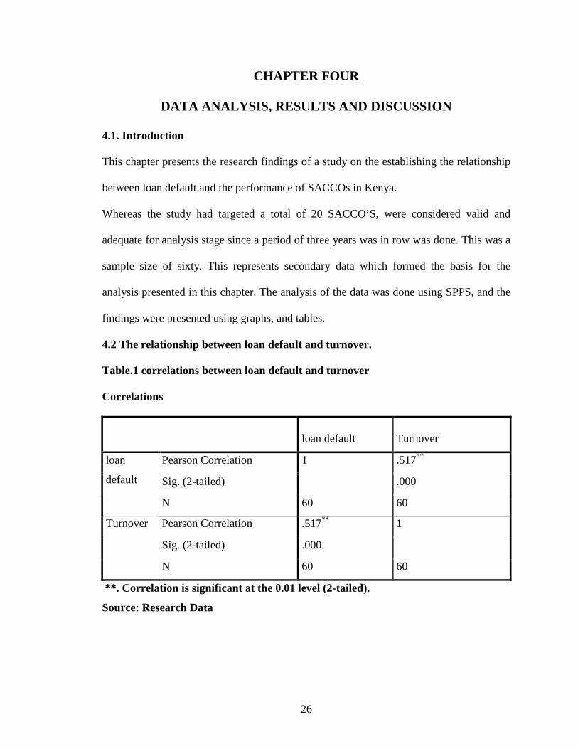
4.2 The relationship between loan default and turnover.

Table.1 correlations between loan default and turnover

Correlations

loan default Turnover

Pearson Correlation 1 .517**

Sig. (2-tailed) .000

loan

default

N 60 60

Pearson Correlation .517** 1

Sig. (2-tailed) .000

Turnover

N 60 60

**. Correlation is significant at the 0.01 level (2-tailed).

Source: Research Data

27

From the table above, there exists a moderate correlation between the loan default and

turnover from the sample size of 60 used. This has the potential of interfering with the

liquidity and future borrowers. Since majority of contributions and repayments are used

to advance loans, increase in loan default will hamper the turn over of this SACCO’S.

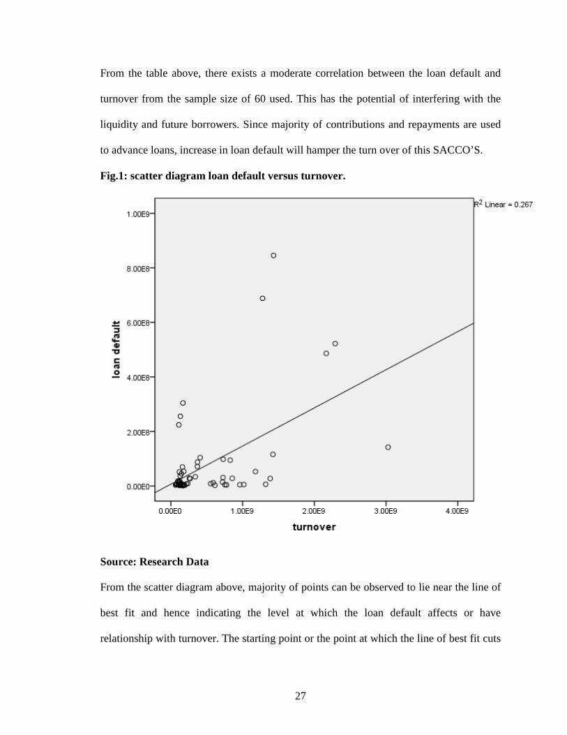
Fig.1: scatter diagram loan default versus turnover.

Source: Research Data

From the scatter diagram above, majority of points can be observed to lie near the line of

best fit and hence indicating the level at which the loan default affects or have

relationship with turnover. The starting point or the point at which the line of best fit cuts

28

the y-axis shows the lowest point of intersection and the point they share.

Table.2: model summary of the correlations between loan default and the turnover.

Model Summary

Model

R

R

Squar

e

Adjusted

R Square

Std. Error

of the

Estimate Durbin-Watson

dimension0

1 .517a .267 .254 5.29858E8 1.334

a. Predictors: (Constant), loan default

b. Dependent Variable: turnover

Source: Research Data

From the table above, the correlation coefficient (R) of 0.517 indicates there excists a

strong correlation between the two variables and a further correlation of

determination.51.7% of variation in turnover can be explained by loan default and vice

versa. As R-squared increases the standard error of estimate will decrease, and better line

of best fit hence less estimation error.

29

4.3: Relationship between loan default and Assets

Table.3: correlations between loan default and Assets

Correlations

loan default Assets

Pearson Correlation 1 .607**

Sig. (2-tailed) .000

loan

default

N 60 60

Pearson Correlation .607** 1

Sig. (2-tailed) .000

Assets

N 60 60

**. Correlation is significant at the 0.01 level (2-tailed).

Source: Research Data

From the table above, there exists a strong correlation of 0.607 between the loan default

and assets from the sample size of 60 used. This has the potential of interfering with the

liquidity and future borrowing of the company from the Bankers. Increase in assets will

be used as source of collateral by the SACCO’S to source for more finance and hence

advance to its members.

30

Fig.2: scatter diagram loan default versus assets

Source: Research Data

From the scatter diagram above, majority of points can be observed to lie near the line of

best fit and hence indicating the level at which the loan default affects or have

relationship with assets. The starting point or the point at which the line of best fit cuts

the y-axis shows the lowest point of intersection and the point they share.

31

4.4 Relationship between loan default and equity

Table.4: correlations between loan default and equity

Correlations

loan

default Equity

Pearson Correlation 1 .443**

Sig. (2-tailed) .000

loan

default

N 60 60

Pearson Correlation .443** 1

Sig. (2-tailed) .000

Equity

N 60 60

**. Correlation is significant at the 0.01 level (2-tailed).

Source: Research Data

From the table above, the correlation coefficient (R) of 0.443 indicates there exists a

strong correlation between the two variables and a further correlation of

determination.51.7% of variation in turnover can be explained by loan default and vice

versa. As R-squared increases the standard error of estimate will decrease, and better line

of best fit hence less estimation error.

32

Fig.3: scatter diagram loan default versus assets

Source: Research Data

From the scatter diagram above, majority of points can be observed to close the line of

best fit and hence indicating the level at which the loan default affects or have

relationship with Equity. The starting point or the point at which the line of best fit cuts

the y-axis shows the lowest point of intersection and the point they share.

33

4.5 Summary of variables

Table.5: Summary of correlations of variables

Correlations

turnover Assets Equity loan default Membership

Turnover 1.000 .966 .309 .517 .706

Assets .966 1.000 .436 .607 .834

Equity .309 .436 1.000 .443 .646

loan default .517 .607 .443 1.000 .714

Pearson Correlation

Membership .706 .834 .646 .714 1.000

Turnover . .000 .008 .000 .000

Assets .000 . .000 .000 .000

Equity .008 .000 . .000 .000

loan default .000 .000 .000 . .000

Sig. (1-tailed)

Membership .000 .000 .000 .000 .

Source: Research Data.

From the table above, we can see all five variables are correlated with criterion-and all

the correlation is positive. There exist a very strong correlation between turnover and

assets with 0.966, meaning that 96% of assets can be explained by variation in turnover.

Correlation between loan default and other variable are .517 between turnover, 0607 with

assets, 0.443 between equity and 0.714 with membership. From the above table, we can

also deduce more. There exists a strong relationship between assets and members while

also a strong correlation exists between membership and loan default.

34

4.6 Analysis of no variance

Table.6: Analysis of no variance

ANOVA

Model Sum of Squares df Mean Square F Sig.

Regression 2.148E19 4 5.370E18 401.288 .000a

Residual 7.361E17 55 1.338E16

1

Total 2.222E19 59

a. Predictors: (Constant), Equity, Assets, loan default, Membership

b. Dependent Variable: turnover

Source: Research Data

From the table above, “sig” which checks the goodness of fit of the model, shows model

fits the data. Since the significance is less than the 0.05, the goodness of the model is fit.

The model explains the deviations in the dependent variable at 95% confidence interval

and hence we can accept the model and the lower the number the better the fit. Typically,

if Significance could have been greater than 0.05, could have concluded that our model

could not fit the data. The F-ratio in the ANOVA table above tests whether the overall

regression model is a good fit for the data. The table shows that the independent variables

statistically significantly predict the dependent variable, F (4, 95) = 401.288, p < .0005

(i.e., the regression model is a good fit of the data).

35

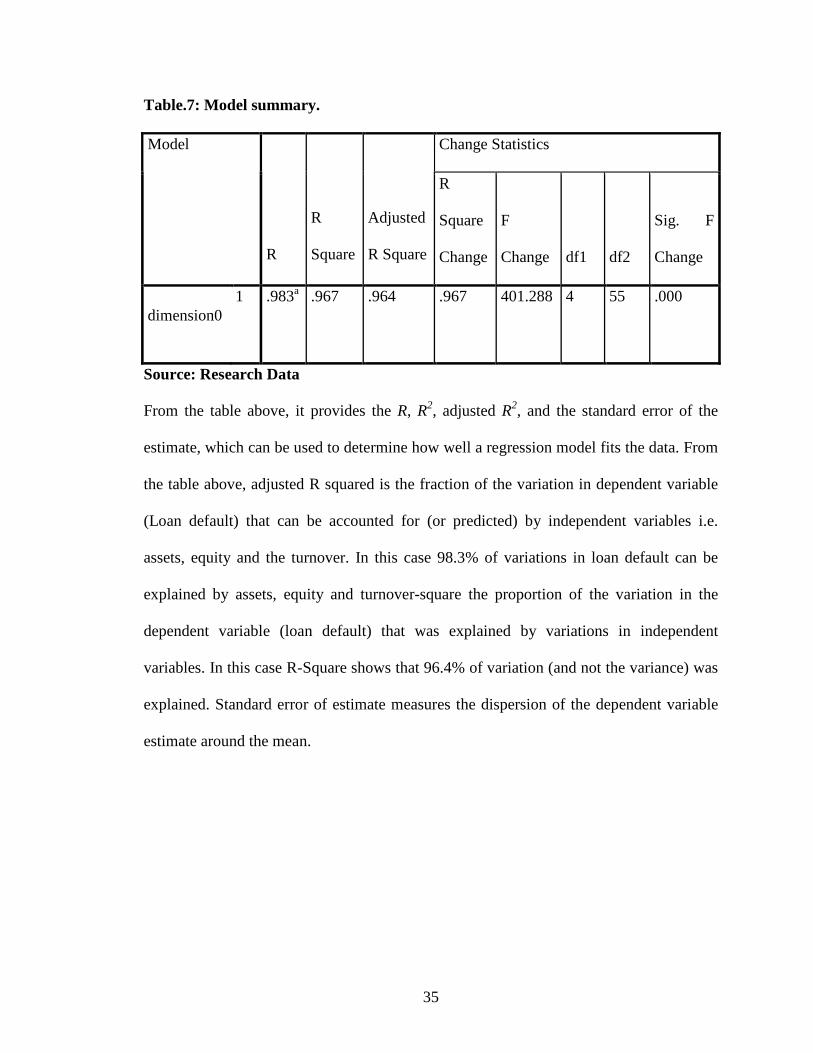
Table.7: Model summary.

Change Statistics Model

R

R

Square

Adjusted

R Square

R

Square

Change

F

Change df1 df2

Sig. F

Change

dimension0 1 .983a .967 .964 .967 401.288 4 55 .000

Source: Research Data

From the table above, it provides the R, R2, adjusted R2, and the standard error of the

estimate, which can be used to determine how well a regression model fits the data. From

the table above, adjusted R squared is the fraction of the variation in dependent variable

(Loan default) that can be accounted for (or predicted) by independent variables i.e.

assets, equity and the turnover. In this case 98.3% of variations in loan default can be

explained by assets, equity and turnover-square the proportion of the variation in the

dependent variable (loan default) that was explained by variations in independent

variables. In this case R-Square shows that 96.4% of variation (and not the variance) was

explained. Standard error of estimate measures the dispersion of the dependent variable

estimate around the mean.

36

Table.8: Model coefficients

Coefficients

Unstandardized

Coefficients

Standardize

d

Coefficients

95.0% Confidence Interval

for B

Model

B Std. Error Beta t Sig.

Lower

Bound

Upper

Bound

(Constant) 1.605E7 2.136E7 .752 .456 -2.675E7 5.886E7

loan

default

-.013 .130 -.003 -.099 .922 -.273 .247

Membershi

p

-8009.862 1644.552 -.290 -4.871 .000 -11305.617 -4714.107

Assets .145 .005 1.227 26.741 .000 .134 .156

1

Equity -.224 .198 -.038 -1.132 .262 -.620 .172

Dependent Variable: turnover

Source: Research Data.

Unstandardized coefficients indicate how much the dependent variable varies with an

independent variable, when all other independent variables are held constant. Consider

the effect of membership in this example. The unstandardized coefficient for assets is

0.145. This means that for each 1 shilling increase in assets, there is a increase in

turnover of 0.145.The general form of the equation to predict turnover from assets,

equity, loan default and membership is:

Predicted Dependant = 16,050,000+ (0.145 x Assets) - (0.224 x Equity) - (0.8009.8 x

membership) - (0.130xloan default).

This is obtained from the Coefficients table, as shown above. In multiple linear

37

regression, the size of the coefficient for each independent variable gives you the size of

the effect that variable is having on your dependent variable, and the sign on the

coefficient (positive or negative) gives you the direction of the effect. In regression with

multiple independent variables, the coefficient tells you how much the dependent variable

is expected to increase when that independent variable increases by one, holding all the

other independent variables constant. From the analysis above and the model, an increase

in loan default cause a decrease in turnover as indicated by the negative sign before the

loan default in the regression model.

The F-ratio in the table 6, tests whether the overall regression model is a good fit for the

data. The table shows that the independent variables statistically significantly predict the

dependent variable, F (4, 95) = 401.288, p < .0005 (i.e., the regression model is a good fit

of the data).

4.7 Summary and Interpretation of the Findings

There exists a moderate correlation between the loan default and turnover from the

sample size of 60 used. This has the potential of interfering with the liquidity and future

borrowers. Since majority of contributions and repayments are used to advance loans,

increase in loan default will hamper the turnover of this SACCO’S.

The model is good as it fits the data and can used to explain the dependent variable as

seen in the ANOVA table. There exists a strong correlation between the loan default and

assets from the sample size of 60 used. This has the potential of interfering with the

liquidity and future borrowing of the company from the Bankers. Increase in assets will

be used as source of collateral by the SACCO’S to source for more finance and hence

38

advance to its members. the correlation coefficient indicates that there exists a strong

correlation between the two variables and a further correlation of determination of

variation in turnover can be explained by loan default and vice versa. As R-squared

increases the standard error of estimate will decrease, and better line of best fit hence less

estimation error. All five variables are correlated with criterion-and all the correlation is

positive. There exist a very strong correlation between turnover and assets meaning that a

high percentage of assets can be explained by variation in turnover. Correlation between

loan default and other variable are between turnover, assets, between equity and

membership. From the above table, we can also deduce more. There exists a strong

relationship between assets and members while also a strong correlation exists between

membership and loan default.

From the overall regression model, the correlations coefficient and coefficient of

determination o shows the model as fit for the data..The model is good as it fits the data

and can used to explain the dependent variable as seen in the ANOVA table. Multiple

regressions also allows you to determine the overall fit (variance explained) of the model

and the relative contribution of each of the predictors to the total variance explained.

Model Summary table provided the R, R2, adjusted R2, and the standard error of the

estimate, which can be used to determine how well a regression model fits the data:

Logistic Regression

This type of regression is used when the dependent variable is variable dichotomous or

binary i.e. takes only two values. Such data is generated by yes and no responses. It’s

flexible and easy to use. The odds generated permit direct observation of relative

39

importance of each independent variable in predicting the dependent variable. Odds ratios

are used to make statistical inferences fro the population from the sample.

The effects of independent variables differ due to the level of significance “sig”

indicated by coefficient table. A p-value of for membership indicates a good predictor,

while the asset also shows the same p-value. Assets can be associated with the level of

Sacco to borrow more and hence have higher liquidity to advance to its members and

therefore increase the turnover.

Increase in membership would also imply that the increase in the deposits by the

members would also cause the increase the availability of borrowing and capital in the

society. For deposit taking institution, sufficient liquidity, to meet the demands of saving

withdrawals, loan disbursement and operational expenses must be maintained.

Loans are granted from member’s saving and so if they are not paid as per the loan

agreement, then members’ savings are at risk. Best practises require that loans that are

not paid as agreed are considered delinquent the day after the first missed payment. The

entire outstanding loan balance is considered past due. Immediate action should be taken

to control delinquency and collect the loan that is reported past due.

Provisions for loan losses are the fist line of defence to protect members’ savings against

identified risks of losses to the SACCO. Provisioning does not imply that the borrower

has been forgiven. Its prudent SACCO’s recognize probable loss from bad loans.

Although loan may be written off in books, the SACCO must do everything possible to

enforce repayment of the outstanding loan. It’s inappropriate to carry non-performing

40

loans in A Sacco loan book knowing very well that loan is not being repaid as per loan

agreement.

In this study loan default was used as an independent variable in comparison to the

turnover as an indicator of financial performance of SACCOs because factors that lead to

loan default in SACCOs was widely researched (eg Kairu 2009; Uboun 988)

41

CHAPTER FIVE

SUMMARY, CONCLUSION AND RECOMMENDATIONS.

5.1 Summary

The study intended to find the relationship between loan default and the performance of

SACCO’s in Kenya. The information used was collected from the regulatory body

SASRA. From the analysis and data collected the following discussions and

recommendations are made. The analysis was based on the objectives of the study. From

the data there exists a moderate correlation between the loan default and assets from the

sample size of 60 used. This has the potential of interfering with the liquidity and future

borrowing of the company from the Bankers. Increase in assets will be used as source of

collateral by the SACCO’S to source for more finance and hence advance to its members.

Unstandardized coefficients indicate how much the dependent variable varies with an

independent variable, when all other independent variables are held constant. Consider

the effect of membership in this example, the unstandardized coefficient for assets. This

means that for each shilling increase in assets, there is a increase in turnover. The general

form of the equation is to predict turnover from assets, equity, loan default and

membership and there is strong correlation between the loan default and turnover from

the sample size of 60 used. This has the potential of interfering with the liquidity and

future borrowers. Since majority of contributions and repayments are used to advance

loans, increase in loan default will hamper the turnover of this SACCO’S.

There exist a very strong correlation between turnover and assets meaning that assets can

42

be explained by variation in turnover. There exists Correlation between loan default and

other variables including turnover, assets, equity and membership. From the above table,

we can also deduce more. There exists a strong relationship between assets and members

while also a strong correlation exists between membership and loan default.

There exists a strong correlation between the loan default and assets from the sample size

of used. This has the potential of interfering with the liquidity and future borrowing of the

company from the Bankers. Increase in assets will be used as source of collateral by the

SACCO’S to source for more finance and hence advance to its members.

5. 2.Conclusions

Based on the results from data analysis and findings the study came up with the following

conclusions. The F-ratio in the table 6, tests whether the overall regression model is a

good fit for the data. The table shows that the independent variables statistically

significantly predict the dependent variable, (i.e., the regression model is a good fit of the

data).

R, R2, and adjusted R2, was used to determine the strength and direction of relation

between these variables. From the table above, Table.7: Model summary. Adjusted R

squared is the fraction of the variation in dependent variable (Loan default) that can be

accounted for (or predicted) by independent variables i.e. assets, equity and the turnover.

In this case variations in loan default can be explained by assets, equity and turnover-

square the proportion of the variation in the dependent variable (loan default) that was

explained by variations in independent variables. In this case R-Square shows variation

(and not the variance) was explained. Standard error of estimate measures the dispersion

43

of the dependent variable estimate around the mean.

The study was to establish if there was relationship between loan default and the

performance of SACCOs in Kenya.From the analysis above and the model, an increase in

loan default cause a decrease in turnover as indicated by the negative sign before the loan

default in the regression model. From the findings it was deduced that in correlation

matrix table there is moderate correlation between loan default and the turnover which

explains the profitability in Sacco’s. From the table of coefficients, loan default shows a

negative effect..This confirms the relationship loan default has on the turnover and the

overall profitability of these Sacco’s.

5.3 Policy Recommendations

In regression with multiple independent variables, the coefficient explains how much the

dependent variable is expected to increase when that independent variable increases by

one, holding all the other independent variables constant. From the analysis above and

the model, an increase in loan default cause a decrease in turnover as indicated by the

negative sign before the loan default in the regression model. SACCO’s should put

stringent measures such as increasing the number of guarantors, reducing the borrowing

factor as well as ensuring insurance covers for large loans. This will go hand in hand in

increasing profitability and with good management it will facilitate increase in return on

assets and equity.

The loans policy should be intended to provide direction, guidelines and make provisions

for proper and efficient utilization and administration of the society’s loan portfolio in

44

order to ensure that the society’s interests are adequately protected to ensure equitable

distribution of funds, encourage liquidity planning and reduce loan default.

Members should not be allowed to withdraw part of his/her deposits or offset part of the

deposits against an outstanding loan unless he/she ceases to be a member. These enhance

loan repayment and reduce loan default. If loan repayment is delayed, the guarantors

should be informed of this fact and be notified that they will be called upon to honor

their obligations if no repayments are effected at the end of a given period. The General

Manager as the CEO of SACCO’S should maintain an up-to-date documentation of loan

files and ensure that loan application form and security are in place in case of arbitration

and suit.

SACCOS should also join the credit reference bureau and educate their members the

need of prompt payment. CRB allows for credit information sharing among the financial

institutions. Credit information sharing undoubtedly plays a pivotal role in reducing the

information asymmetry that exists between banks and borrowers. The major benefit that

the SACCO would receive from CRB is that they would be able to get credit information

on prospective borrowers that will facilitate assessment of credit requests to mitigate

risks of bad debts. On the side of the borrower, a good credit record acts as an incentive

for competitive pricing of loan facilities.

5.4. Limitations of the study

Owing to time and resource limits the study drew its sample only from only 20 SACCOS

in Kenya in spite of thousands .Currently the number of Sacco’s in Kenya has increased

45

drastically and more so after the introduction of transport Sacco’s to help and manage the

transport sector. Majority of these Sacco’s have no up to date information in the SASRA

offices.The study didn’t include many other parameters that affect the performance of

SACCO societies in Kenya due to the nature of information available from the Sacco’s

and the financial constraints narrowing the research to the chosen Sacco’s.

Due to unavailability of information the study didn’t include all the SASRA regulate

SACCOs but only 20 was chosen to be representative. The data used was only from those

SACCO’s that was readily available from the SASRA and for period of three years

continues. Majority of Sacco’s in Kenya have very scanty information in the office of

regulator. This hindered the extent of study. Quality of data provided regarding

membership creates a sense as to the source of this data. For instance, Harambee Sacco

provided same membership number in year 2010 and 2011 which makes one doubt this

data.

5.5. Recommendations for further research

This study was to establish if there was relationship between loan default and the

performance of SACCOs in Kenya.Personality types are predisposed to loan default. To

this end therefore accurately identifying these personality types could have profound

implications for consumer policy, and also important lessons for our understanding of

why credit markets may fail. Reason behind non-repayment of loan, mis -use or the past

trends of these loan defaults can be analyzed.

Further research can be done to confirm the relationship between the impact of growth in

assets and how its related to the return in assets, and the impact of government

46

regulations on the performance and management of SACCO’s as more and more

SACCO’S continue to be formed in different sectors.

The study didn’t include many of other parameters that affect the performance of

SACCO societies in Kenya. Such other parameters include the economic environment,

literacy levels of the members, the sector under which the members are derived from.

This would check the nature and culture of saving in these Sacco’s.

It is recommended that further research should be done on need for provision of training

to the members since investment knowledge helps one to make better decisions on how to

invest loans. This might help SACCO’s ensure that business education programmers’

focus more on entrepreneurship training to prepare members for investment and to

increase their capacity for future learning. It would help recognize the competences

required for members to seek or gain advantage in funds allocated. There is a need for the

SACCO members to take proper business analysis before investment in order to reduce

the effects of policies, poverty levels, culture/ beliefs the nature of investment system and

inflation rate as factors which greatly affects the rate of return on investment of loans.

Further, the SACCO management should provide additional training on employee

relations since employee participation, quality system, employee training continuous

support, information and analysis, top management commitment and support and

customer focused reduce the level of risk of loans in SACCO’s. The SACCO should also

revise its lending policies to ensure that more members no idle funds and limiting

members with huge contributions

47

REFERENCES

Allen, .E & Maghimbi, S. (2009) African cooperatives and the financial crisis; Coop

AFRICA Working Paper No.3

AMFIU Report (2008): Microfinance Tomorrow: Refocusing the vision for the Industry

in Uganda; An Analytical booklet for the proceedings of the 2008 AMFIU Pre

AGM Workshop.

Basurto, M. Goodhart, Hofman, B., ( 2006) Default Credit Growth,.and asset prices.

IMF working paper wp/06/223,Sept 2006

BOU (2003), “Economic and Financial indicators” Monthly Economic Report,Kampala

Chambo S. A. 2006. Co-operating out of poverty in Tanzania. ILO conference 6th to

10th February 2006. Pretoria South Africa

Chirwa, E.A., (1997). “An econometric analysis of the determinants of agricultural credit

payment in Malawi,” African Review of Money Finance and Banking, Vol. 1-2:

Corporate Social responsibility, and financial performance measures. JB McGuive, a

Sundgren, T Schneewels, (1988).

David , M. (2011) Loan default pose risk to Sacco Financial Stability. Business Daily

June 2011

Embrechts , McNell 2003 Credit Risk models,multivariate models for portfolio credit

risk.

Firzli, M. ,Nicolas, J. (2010) Greece and roots the EU crisis

Goto D. H. 2004. Financial mismanagement of Nyati SACCO. Unpublished MBA

research project. in Kenya

48

Jensen investment management (2008) ‘why return on equity is a useful criterion for

equity selection’

Joetta, (2007) credit risk management: ‘‘how to avoid lending disasters and maximize

earnings’’, third edition

Joel, Bessis (1998) “Risk management in Banking”,John Wiley & sons ,1998

Karlinger ,F.N. (1986) “Foundation of behavioural Research”, (3rd edition)

Keenan, S. (1999) Historical default rates of corporate bonds issues 1920-1998.Moods

investor service ,Global Credit Research, January 1999

Kithunzi.M .(2009). Effectiveness of guarantorship in loan recovery in cooperative

societies in Kenya: Case study of Mwalimu Sacco.Upublished university of

Nairobi

Kothari, 2004. Research methodology. Methods and techniques. New Age International

Ltd, New Delhi, India.

Lando and David (2004) Credit risk modeling theory and application –Princeton

University Press

Manyara K. M., 2004, Co-operative Law in Kenya. Rock Graphics, Nairobi Kenya.

Mwangi (2012) Effect of credit risk management on the financial performance of

Commercial Banks

Mugenda,O.M. A.G.(2003) “Research methods “ Lab Graphics, Nairobi Kenya.

Mugwanga 1999. Use and impact of Savings services for poor people in Kenya. A

research paper for AERC.

49

Merton, Robert C,. (1974) “ on the pricing of corporate debt:The risk structure of

corporate bonds “, Journal of Finance , 2,449-471

Mukenda ,O.M.and Mukenda A.G.(1999) “Research methods :Quantitative and

Qualitative approaches”, Nairobi, Acts press

Nabangi, T. 2005: Assessment of factors that affect cash flows of savings and credit

societies in Nairobi. Unpublished MBA research project. School of business and

Management Moi University. Nairobi, Kenya.

Narayan 1997. Voices of the poor. Poverty and social capital in Tanzania. World Bank.

Omweri L, 1998. An investigation of members attitudes as regards the lending policies

for savings and credit co-operatives in Kenya. A case of Mwalimu Sacco Society.

Unpublished MBA Kenyatta University.

Oswaldo C. P. 2001. National Survey of Credit Unions Ecuador. WOCCU Inc.

Ouma J. S, 1990, The transformation of the informal sector. The co-operative

perspective. Shirikon Press, Nairobi.

Republic of Kenya 1997, Co-operatives Societies Act. 12.

Republic of Kenya 1997, Retirements Benefits Act No. 2

Ronald.K.S (2011) The effect of change in capital structure in the financial performance

of SACCOs in Nairobi.Upublished MBA University of Nairobi

Rutkowski M (1999), Models of default risk.

Sadakkadulla .J & Subbaiah,S. (2002) “ performance measure for Banks” ,Financial

50

Daily ,The Hindu Group Of Publication.

Steams K, 1991, Methods for Managing delinquency. Tools formicro-enterprise

programmes, Germinii Technical series USA.

Sullivan, Eurtur, Steven M Sheffrin (2003), Economic Principles in Action.

Van Horn J C (1998) ‘‘Financial Management and policy’’prentice hall 11th Ed,upper

Saddle River New Jersey

51

APPENDICES

APPENDIX I: List of Licenced SACCOs by Sacco Society Regulatory Authority as

at 31st December 2012

1. Ardhi

2. Elimu

3.Lenga

4. Tumaini

5. Nest

6. Reli

7. Teleposta

8. Transcom

10.Ufanisi

11. Ufundi

12. Ukristo na Ufanisi

13. Afya

14. Airports

15. Asili Cooperative

16. Chai

17. Chuna

17. Comoco

18. Fundlima

19. Harambee

20. Hazina

21Jamii

22. Kenpipe

23. Kenversity

24. Kenya Bankers

25. Kenya Police

26. Kingdom

27. Magereza

52

28. Maisha Bora

29. Mwalimu National

30.Mwito

31Nacico

32.Nafaka

33.Naku

34.Nassefu

35.Nation Staff

36.Orthodox

37.Safaricom

38.Sheria

39.Stima

40.Tembo

41.Ukulima

42.United nations

43.Wanaanga

44.Wanandege

45.Waumini

Source: SASRA Records

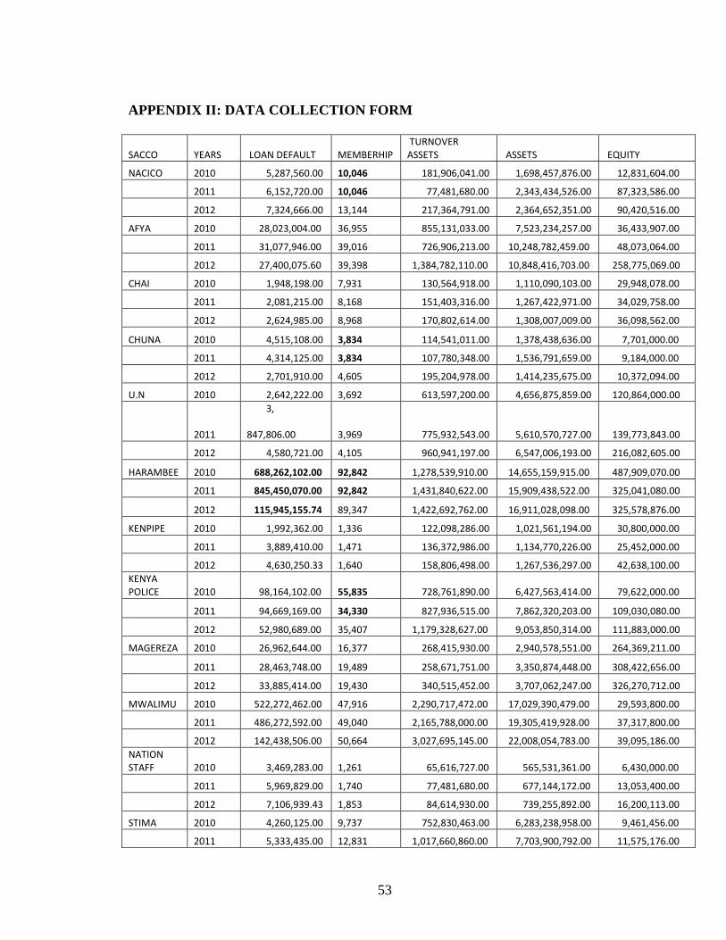
53

APPENDIX II: DATA COLLECTION FORM

SACCO YEARS LOAN DEFAULT MEMBERHIP

TURNOVER

ASSETS ASSETS EQUITY

NACICO 2010 5,287,560.00 10,046 181,906,041.00 1,698,457,876.00 12,831,604.00

2011 6,152,720.00 10,046 77,481,680.00 2,343,434,526.00 87,323,586.00

2012 7,324,666.00 13,144 217,364,791.00 2,364,652,351.00 90,420,516.00

AFYA 2010 28,023,004.00 36,955 855,131,033.00 7,523,234,257.00 36,433,907.00

2011 31,077,946.00 39,016 726,906,213.00 10,248,782,459.00 48,073,064.00

2012 27,400,075.60 39,398 1,384,782,110.00 10,848,416,703.00 258,775,069.00

CHAI 2010 1,948,198.00 7,931 130,564,918.00 1,110,090,103.00 29,948,078.00

2011 2,081,215.00 8,168 151,403,316.00 1,267,422,971.00 34,029,758.00

2012 2,624,985.00 8,968 170,802,614.00 1,308,007,009.00 36,098,562.00

CHUNA 2010 4,515,108.00 3,834 114,541,011.00 1,378,438,636.00 7,701,000.00

2011 4,314,125.00 3,834 107,780,348.00 1,536,791,659.00 9,184,000.00

2012 2,701,910.00 4,605 195,204,978.00 1,414,235,675.00 10,372,094.00

U.N 2010 2,642,222.00 3,692 613,597,200.00 4,656,875,859.00 120,864,000.00

2011

3,

847,806.00 3,969 775,932,543.00 5,610,570,727.00 139,773,843.00

2012 4,580,721.00 4,105 960,941,197.00 6,547,006,193.00 216,082,605.00

HARAMBEE 2010 688,262,102.00 92,842 1,278,539,910.00 14,655,159,915.00 487,909,070.00

2011 845,450,070.00 92,842 1,431,840,622.00 15,909,438,522.00 325,041,080.00

2012 115,945,155.74 89,347 1,422,692,762.00 16,911,028,098.00 325,578,876.00

KENPIPE 2010 1,992,362.00 1,336 122,098,286.00 1,021,561,194.00 30,800,000.00

2011 3,889,410.00 1,471 136,372,986.00 1,134,770,226.00 25,452,000.00

2012 4,630,250.33 1,640 158,806,498.00 1,267,536,297.00 42,638,100.00

KENYA

POLICE 2010 98,164,102.00 55,835 728,761,890.00 6,427,563,414.00 79,622,000.00

2011 94,669,169.00 34,330 827,936,515.00 7,862,320,203.00 109,030,080.00

2012 52,980,689.00 35,407 1,179,328,627.00 9,053,850,314.00 111,883,000.00

MAGEREZA 2010 26,962,644.00 16,377 268,415,930.00 2,940,578,551.00 264,369,211.00

2011 28,463,748.00 19,489 258,671,751.00 3,350,874,448.00 308,422,656.00

2012 33,885,414.00 19,430 340,515,452.00 3,707,062,247.00 326,270,712.00

MWALIMU 2010 522,272,462.00 47,916 2,290,717,472.00 17,029,390,479.00 29,593,800.00

2011 486,272,592.00 49,040 2,165,788,000.00 19,305,419,928.00 37,317,800.00

2012 142,438,506.00 50,664 3,027,695,145.00 22,008,054,783.00 39,095,186.00

NATION

STAFF 2010 3,469,283.00 1,261 65,616,727.00 565,531,361.00 6,430,000.00

2011 5,969,829.00 1,740 77,481,680.00 677,144,172.00 13,053,400.00

2012 7,106,939.43 1,853 84,614,930.00 739,255,892.00 16,200,113.00

STIMA 2010 4,260,125.00 9,737 752,830,463.00 6,283,238,958.00 9,461,456.00

2011 5,333,435.00 12,831 1,017,660,860.00 7,703,900,792.00 11,575,176.00

54

2012 6,349,328.00 14,977 1,321,818,000.00 9,402,400,000.00 14,329,505.00

SHERIA 2010 37,298,140.00 6,255 129,274,580.00 1,248,585,274.00 6,219,900.00

2011 44,944,794.00 6,255 147,052,475.00 1,634,614,030.00 35,073,724.00

2012 53,505,707.00 8,146 180,314,622.00 2,324,091,802.00 5,753,750.00

UKULIMA 2010 8,511,244.00 27,749 555,382,388.00 4,606,350,618.00 137,309,110.00

2011 12,022,538.00 33,847 589,815,479.00 5,080,073,524.00 56,785,400.00

2012 14,312,545.00 34,296 721,297,435.00 6,547,006,193.00 141,963,500.00

WANA-

NDEGE 2010 12,222,412.00 1,190 129,544,016.00 1,044,871,557.00 3,880,000.00

2011 10,355,619.00 4,194 141,028,594.00 1,206,286,516.00 4,318,000.00

2012 1,072,931.00 5,014 168,803,359.00 1,204,999,335.00 62,858,451.00

KENYA

BANKERS 2010 71,252,106.00 16,565 369,555,535.00 4,109,947,723.00 82,825,000.00

2011 87,565,978.00 16,565 370,224,003.00 4,287,259,898.00 87,380,000.00

2012 104,245,212.00 27,847 408,560,155.00 4,849,098,277.00 92,195,000.00

SAFARICOM 2010 16,118,250.00 2,230 102,513,303.00 792,870,636.00 10,741,422.00

2011 18,242,207.00 2,430 97,487,488.00 958,130,542.00 13,192,776.00

2012 18,387,666.00 3,108 121,804,527.00 1,064,033,767.00 5,914,695.00

JAMII 2010 51,248,110.00 10,493 117,579,174.00 1,079,349,412.00 25,769,090.00

2011 69,879,245.00 11,954 161,587,784.00 1,271,286,978.00 42,586,113.00

2012 9,181,037.00 14,180 236,155,902.00 1,521,935,447.00 56,787,581.00

WAUMINI 2010 224,522,110.00 12,277 110,925,876.00 1,149,361,057.00 51,114,472.00

2011 255,810,304.00 13,407 132,365,464.00 1,386,326,947.00 55,232,214.00

2012 304,536,076.00 14,691 167,944,123.00 1,204,999,335.00 60,803,641.00

WANANGA 2010 4,250,114.00 1,990 99,354,713.00 603,811,524.00 5,970,000.00

2011 6,880,319.00 2,048 127,980,763.00 812,605,516.00 20,634,800.00

2012 8,190,856.00 2,477 138,138,899.00 911,362,906.00 27,486,350.00

SOURCE: SASRA 2012